Marine magnetotellurics for base-of-salt mapping: Gulf of

GEOPHYSICS, VOL. 65, NO. 5 (SEPTEMBER-OCTOBER 2000); P. 1476–1488, 17 FIGS.

Marine magnetotellurics for base-of-salt mapping:Gulf of Mexico field test at the Gemini structure

G. Michael Hoversten∗, Steven C. Constable‡, and H. Frank Morrison∗∗

ABSTRACT

A sea-floor magnetotelluric (MT) survey was con-ducted over the Gemini subsalt petroleum prospect inthe Gulf of Mexico (GOM) to demonstrate that thebase of salt can be mapped using marine magnetotelluric(MMT) methods. The high contrast in electrical resistiv-ity between the salt and the surrounding sediments pro-vides an excellent target for MMT. The Gemini salt body,located at 28◦ 46′ N 88◦ 36′ W, is a relatively complexshape buried 2–5 km below the sea floor in 1-km-deepwater. Its geometry has been previously determined us-ing 3-D seismic prestack depth migration with well logcontrol. In order not to confuse limitations in interpre-tation technique with limitations in data acquisition, nu-merical forward and inverse modeling guided the sur-vey design to locate a profile that would be amenableto 2-D inversion, even though the body was clearly 3-D.The seismic imaging of the base of salt along the cho-sen profile is considered good, thus providing a goodcontrol for testing the MT method. In many other areasof the GOM, and indeed other portions of the Geministructure itself, seismic imaging of the base of salt is prob-lematic. Data were collected using autonomous sea-floordata loggers equipped with induction coil magnetic sen-sors and electric field sensors consisting of silver–silverchloride electrodes connected to an ac-coupled amplifieroriginally designed for sea-floor controlled-source stud-ies. Nine sites of excellent quality MT responses wereobtained. Smooth 2-D inversion of the data produce aconfined resistive anomaly at the correct location anddepth, and recently developed sharp-boundary 2-D in-version recovers base of salt in excellent agreement withthe seismic models. Simple perturbation analysis showsthat base of salt has been resolved to within 5–10% ofburial depth.

Presented at the 68th Annual International Meeting, Society of Exploration Geophysicists. Manuscript received by the Editor August 17, 1998;revised manuscript received March 24, 2000.∗Lawrence Berkeley National Laboratory, One Cyclotron Road, MS 90-1116, Berkeley, California 94720. E-mail: [email protected].‡Scripps Institution of Oceanography, IGPP 0225, La Jolla, California 92093-0225. E-mail: [email protected].∗∗University of California at Berkeley, 577 Evans Hall, Berkeley, California 94720. E-mail: [email protected]© 2000 Society of Exploration Geophysicists. All rights reserved.

INTRODUCTION

The magnetotelluric (MT) method has been used for manydecades on land to assist in exploration for petroleum (Vozoff,1972; Orange, 1989). It is particularly useful for basin recon-naissance, and in areas where seismic methods perform poorly,such as carbonate and volcanic terrain. In areas where sedi-ments are obscured by rock units that scatter and reflect mostnormal incident seismic energy, electrical methods may be veryhelpful in determining the structural relationships and thick-ness of the various units. It is generally true that rocks with highseismic velocities and impedance contrasts are also higher inelectrical resistance than surrounding sediments.

For these reasons, Hoversten and Unsworth (1994) andHoversten (1992) carried out model studies to test the fea-sibility of using MT methods to map base of salt in the Gulfof Mexico (GOM) and other regions. Salt has a high acousticcontrast with surrounding sediments, which make seismic sec-tions difficult to interpret, and it is much more resistive thanwater-saturated clastic sediments. It was shown that with MTdata of reasonable quality in the 0.001–1 Hz band, the base ofsalt could indeed be mapped with accuracy approaching thatof seismic methods. Unfortunately, however, most marine MTup to that time involved use of long-period instrumentation indeep ocean waters to probe the mantle at depths of 100 kmand deeper (e.g., Filloux, 1983). It was generally believed thatattenuation of the natural EM fields by seawater precludedthe use of MT in the ocean at any significant depth (Chaveet al., 1991). An early attempt to use MT in very shallow wa-ter in the GOM met with limited success (Hoehn and Warner,1960); however, data processing techniques at the time wereunable to remove the large wave-motion noise resulting fromthe experiment’s depth of only 10 m. In addition, the equip-ment was far too bulky to be commercially viable. And be-cause it was a moored system, it would not have been practi-cal in modern prospects where the sea-floor depth approaches2000 m. Traditionally, controlled-source methods have beenused on the sea floor to replace the electromagnetic (EM)

1476

MT for Base-of-Salt Mapping: GOM Field Test 1477

energy lost in the seawater (e.g., Constable and Cox, 1996), andhave been proposed for offshore exploration (Constable et al.,1986).

To overcome the limitations of the existing marine MTmethod, Constable et al. (1998) developed a new generationof marine instrumentation capable of detecting and ampli-fying the weak sea-floor EM signals in the band needed tomap continental shelf structures. A single test deployment offSan Diego, California, in 1995 produced good quality data onthe first attempt and so, in 1996, field trials were carried outin the GOM over both the Mahogany and Gemini subsalt dis-coveries to develop second-generation equipment capable offrequent and repeated deployment. Excellent quality electric-field records were collected from the new instruments, but earlyefforts to record magnetic-field data were frustrated both byinstrument motion in the earth’s large magnetic field and bymagnetic noise generated by fluctuating power consumptionof the nearby logging electronics. To address these problems,logging software and hardware were modified to maintain con-stant power consumption, and the instrument anchor increasedfrom 75 to 200 kg. These changes improved the quality of themagnetic data considerably, and our paper describes resultsfrom a second survey over the Gemini prospect in 1997, de-signed explicitly to show the power of the marine MT (MMT)method to map base of salt economically with a small numberof sea floor stations. The following sections describe the equip-ment, survey design, data acquisition and processing, inversion,and sensitivity analysis.

SEA-FLOOR MT SYSTEM

Constable et al. (1998) give a detailed description of theMT system and the 1995 offshore California test. The MMTinstrument is an autonomous data logging package that free-falls to the sea floor under the weight of an anchor that is laterreleased to allow the otherwise buoyant package to float backto the surface. While a moored system might be more reliableand even collect better quality data, the free vehicle approachhas a big advantage in the time taken to deploy and recover thesystem, especially in deep water. The ship is not encumberedduring the time it takes the instrument to sink to or rise from thesea floor, and so many instrument systems can be deployed torecord simultaneously, which not only increases productivity,it also allows advantage to be taken of modern array-basedprocessing schemes (e.g., Egbert, 1997).

The sea-floor instrument is a modular package composed of adigital data logging system, an acoustic navigation/release unit,electric- and magnetic-field sensors, glass flotation balls, andconcrete anchor, all held together by a largely plastic frame. Ifthe electric and magnetic sensors are replaced by hydrophones,the system can, and has, performed double duty as a sea-floorseismic recorder. The logging system stores 16-bit data to mag-netic disk, and is limited in capacity only by the size of avail-able disk drives, currently 18 GByte. The unit is presently beingupgraded to 24-bit capability. The magnetic sensors are com-mercially available induction coils with an operating band from10 000 s to 1000 Hz, housed in an aluminum pressure case. Theconductive pressure case acts as a high-cut filter with a cornerfrequency around 1 Hz. It is the electric-field sensors, based onthe sea-floor controlled-source EM system described by Webbet al. (1985) and Constable and Cox (1996), that sets this in-

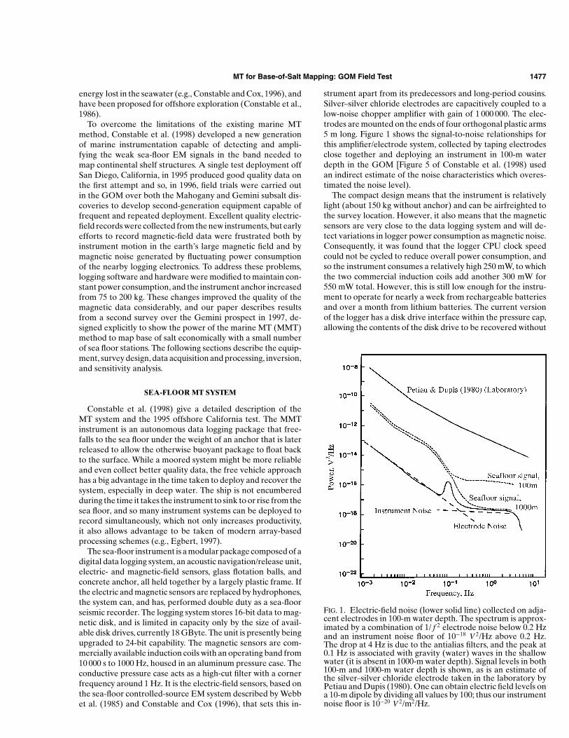
strument apart from its predecessors and long-period cousins.Silver–silver chloride electrodes are capacitively coupled to alow-noise chopper amplifier with gain of 1 000 000. The elec-trodes are mounted on the ends of four orthogonal plastic arms5 m long. Figure 1 shows the signal-to-noise relationships forthis amplifier/electrode system, collected by taping electrodesclose together and deploying an instrument in 100-m waterdepth in the GOM [Figure 5 of Constable et al. (1998) usedan indirect estimate of the noise characteristics which overes-timated the noise level).

The compact design means that the instrument is relativelylight (about 150 kg without anchor) and can be airfreighted tothe survey location. However, it also means that the magneticsensors are very close to the data logging system and will de-tect variations in logger power consumption as magnetic noise.Consequently, it was found that the logger CPU clock speedcould not be cycled to reduce overall power consumption, andso the instrument consumes a relatively high 250 mW, to whichthe two commercial induction coils add another 300 mW for550 mW total. However, this is still low enough for the instru-ment to operate for nearly a week from rechargeable batteriesand over a month from lithium batteries. The current versionof the logger has a disk drive interface within the pressure cap,allowing the contents of the disk drive to be recovered without

FIG. 1. Electric-field noise (lower solid line) collected on adja-cent electrodes in 100-m water depth. The spectrum is approx-imated by a combination of 1/ f 2 electrode noise below 0.2 Hzand an instrument noise floor of 10−18 V 2/Hz above 0.2 Hz.The drop at 4 Hz is due to the antialias filters, and the peak at0.1 Hz is associated with gravity (water) waves in the shallowwater (it is absent in 1000-m water depth). Signal levels in both100-m and 1000-m water depth is shown, as is an estimate ofthe silver–silver chloride electrode taken in the laboratory byPetiau and Dupis (1980). One can obtain electric field levels ona 10-m dipole by dividing all values by 100; thus our instrumentnoise floor is 10−20 V 2/m2/Hz.

1478 Hoversten et al.

opening the pressure case. This improves both the reliability ofthe instrument and speed of redeployment.

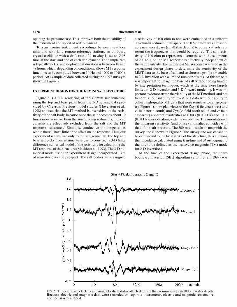
To synchronize instrument recordings between sea-floorunits and with land remote-reference stations, an on-boardcrystal oscillator with a drift rate of 1 ms/day is set to GPStime at the start and end of each deployment. The sample rateis typically 25 Hz, and deployment duration is between 18 and48 hours which, depending on conditions, allows MT responsefunctions to be computed between 10 Hz and 1000 to 10 000 speriod. An example of data collected during the 1997 survey isshown in Figure 2.

EXPERIMENT DESIGN FOR THE GEMINI SALT STRUCTURE

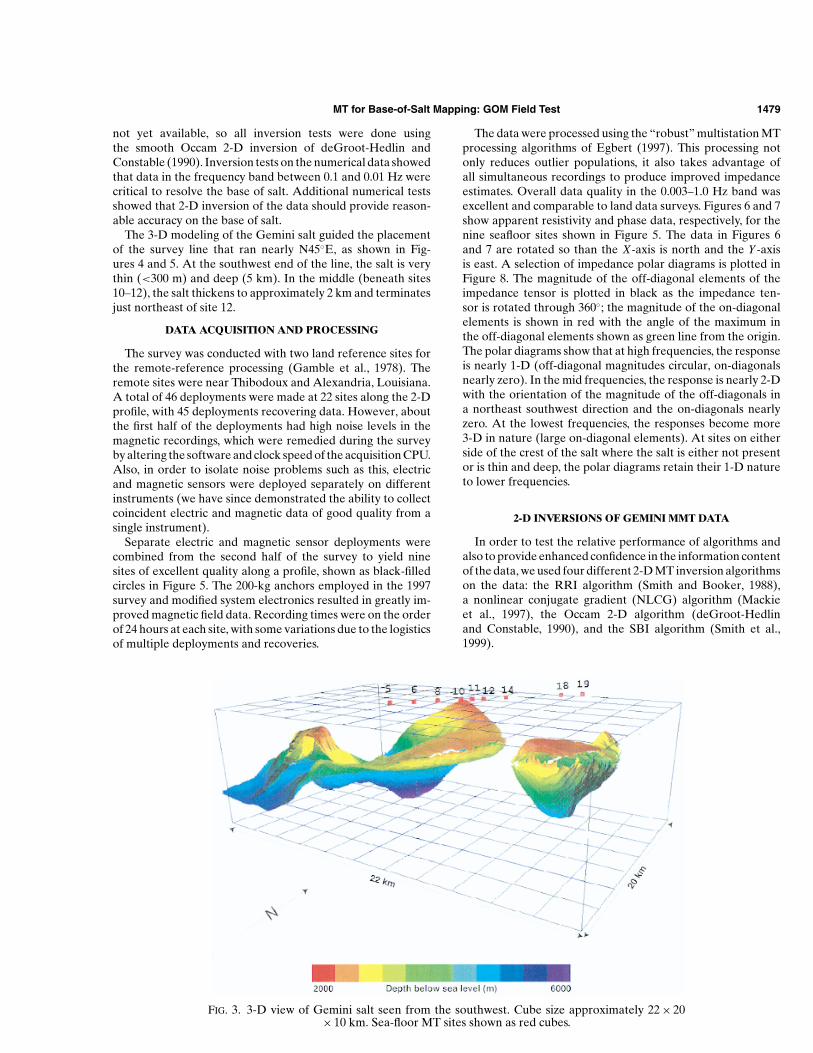
Figure 3 is a 3-D rendering of the Gemini salt structure,using the top and base picks from the 3-D seismic data pro-vided by Chevron. Previous model studies (Hoversten et al.,1998) showed that the MT method is insensitive to the resis-tivity of the salt body, because once the salt becomes about 10times more resistive than the surrounding sediments, inducedcurrents are effectively excluded from the salt and the MTresponse “saturates.” Similarly, conductive inhomogeneitieswithin the salt have little or no effect on the response. Thus, ourexperiment is sensitive only to the salt geometry. The top andbase salt picks from seismic were use to construct a 3-D finitedifference numerical model of the resistivity for calculating theMT response of the structure (Mackie et al., 1993). The 3-D nu-merical model used for experiment design incorporated 1 kmof seawater over the prospect. The salt bodies were assigned

FIG. 2. Time-series of electric- and magnetic-field data collected during the Gemini survey in 1000-m water depth.Because electric and magnetic data were recorded on separate instruments, electric and magnetic sensors arenot necessarily aligned.

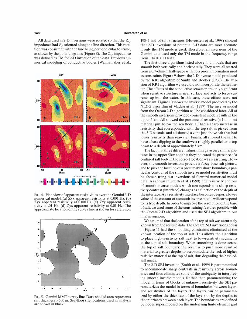
a resistivity of 100 ohm-m and were embedded in a uniform0.5-ohm-m sediment half-space. The 0.5 ohm-m was a reason-able near-worst case (small skin depths) to conservatively rep-resent the frequencies that would be required. The salt resis-tivity of 100 ohm-m represents a contrast with the sedimentsof 200 to 1, so the MT response is effectively independent ofthe salt resistivity. The numerical MT response was used in theexperiment design phase to determine the sensitivity of theMMT data to the base of salt and to choose a profile amenableto 2-D inversion with a limited number of sites. At this stage, itwas important to image the base of salt without being limitedby interpretation techniques, which at the time were largelylimited to 2-D inversion and 3-D forward modeling. It was im-portant to demonstrate the viability of the MT method, and notto confuse our inability to invert 3-D data with our ability tocollect high-quality MT data that were sensitive to salt geome-try. Figure 4 shows plan views of the Zxy (E field east-west andH field north-south) and Zyx (E field north-south and H fieldeast-west) apparent resistivities at 1000 s (0.001 Hz) and 100 s(0.01 Hz) periods along with the survey line. The orientation ofthe apparent resistivity (and phase) anomalies coincides withthat of the salt structure. The 500-m salt isochron map with thesurvey line is shown in Figure 5. The survey line was chosen tobe orthogonal to the local strike of the structure, thus allowingthe impedance calculated using E in-line and H orthogonal tothe line to be defined as the transverse magnetic (TM) modefor 2-D inversions.

At the time of the experiment design phase, the sharpboundary inversion (SBI) algorithm (Smith et al., 1999) was


not yet available, so all inversion tests were done usingthe smooth Occam 2-D inversion of deGroot-Hedlin andConstable (1990). Inversion tests on the numerical data showedthat data in the frequency band between 0.1 and 0.01 Hz werecritical to resolve the base of salt. Additional numerical testsshowed that 2-D inversion of the data should provide reason-able accuracy on the base of salt.

The 3-D modeling of the Gemini salt guided the placementof the survey line that ran nearly N45◦E, as shown in Fig-ures 4 and 5. At the southwest end of the line, the salt is verythin (<300 m) and deep (5 km). In the middle (beneath sites10–12), the salt thickens to approximately 2 km and terminatesjust northeast of site 12.

DATA ACQUISITION AND PROCESSING

The survey was conducted with two land reference sites forthe remote-reference processing (Gamble et al., 1978). Theremote sites were near Thibodoux and Alexandria, Louisiana.A total of 46 deployments were made at 22 sites along the 2-Dprofile, with 45 deployments recovering data. However, aboutthe first half of the deployments had high noise levels in themagnetic recordings, which were remedied during the surveyby altering the software and clock speed of the acquisition CPU.Also, in order to isolate noise problems such as this, electricand magnetic sensors were deployed separately on differentinstruments (we have since demonstrated the ability to collectcoincident electric and magnetic data of good quality from asingle instrument).

Separate electric and magnetic sensor deployments werecombined from the second half of the survey to yield ninesites of excellent quality along a profile, shown as black-filledcircles in Figure 5. The 200-kg anchors employed in the 1997survey and modified system electronics resulted in greatly im-proved magnetic field data. Recording times were on the orderof 24 hours at each site, with some variations due to the logisticsof multiple deployments and recoveries.

FIG. 3. 3-D view of Gemini salt seen from the southwest. Cube size approximately 22 × 20× 10 km. Sea-floor MT sites shown as red cubes.

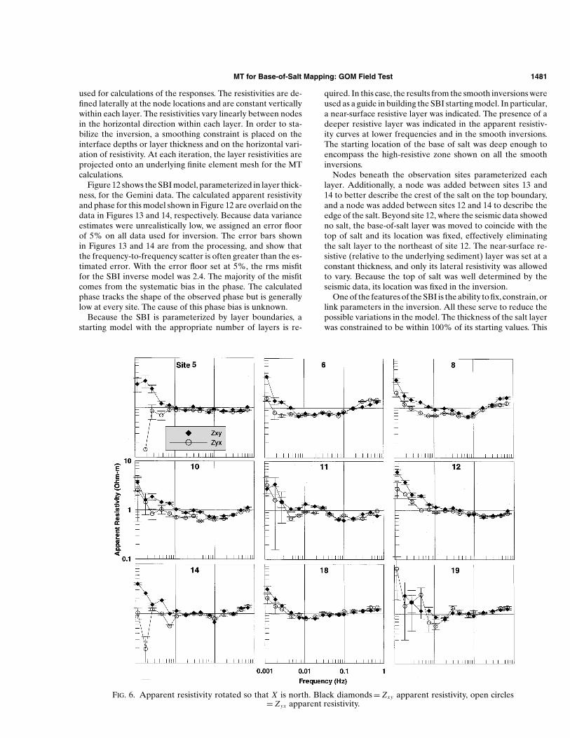
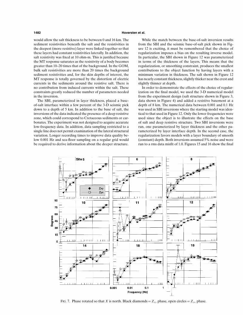
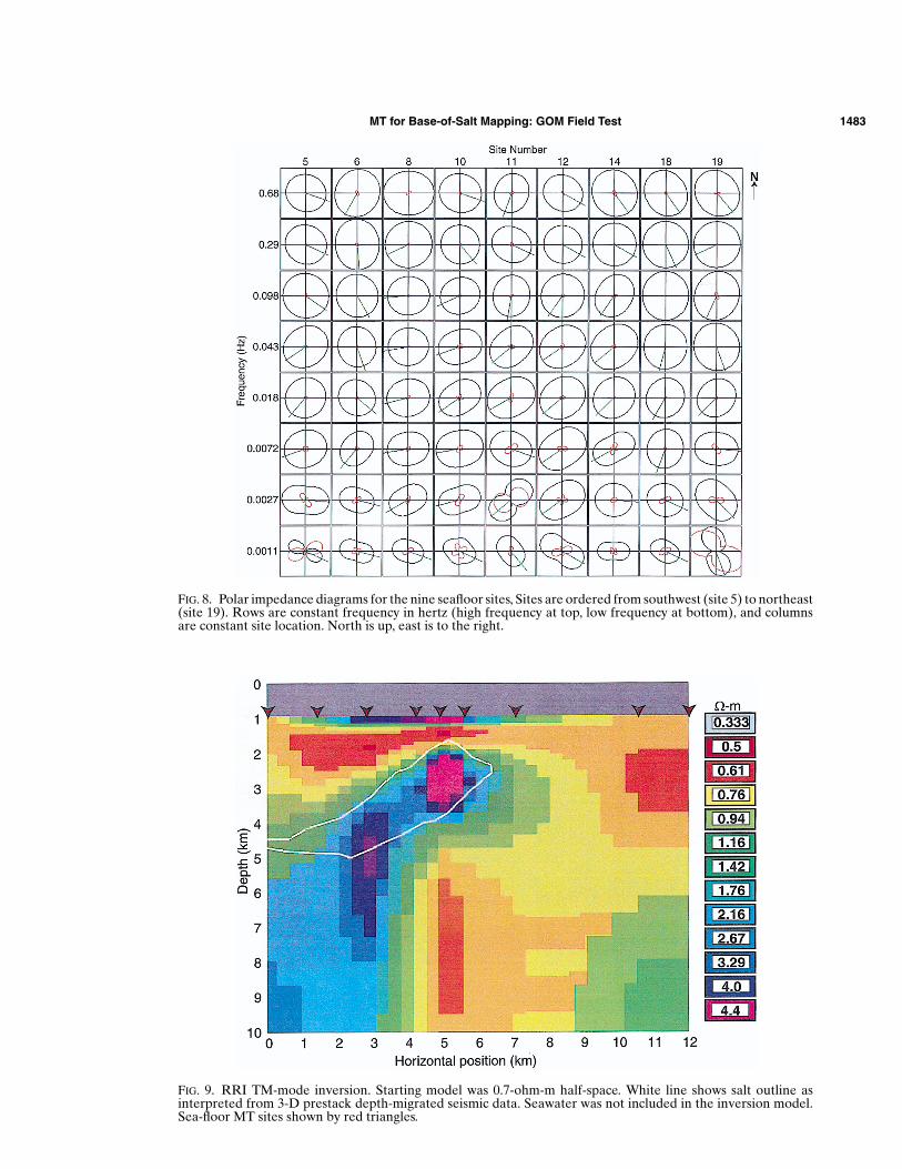
The data were processed using the “robust” multistation MTprocessing algorithms of Egbert (1997). This processing notonly reduces outlier populations, it also takes advantage ofall simultaneous recordings to produce improved impedanceestimates. Overall data quality in the 0.003–1.0 Hz band wasexcellent and comparable to land data surveys. Figures 6 and 7show apparent resistivity and phase data, respectively, for thenine seafloor sites shown in Figure 5. The data in Figures 6and 7 are rotated so than the X -axis is north and the Y -axisis east. A selection of impedance polar diagrams is plotted inFigure 8. The magnitude of the off-diagonal elements of theimpedance tensor is plotted in black as the impedance ten-sor is rotated through 360◦; the magnitude of the on-diagonalelements is shown in red with the angle of the maximum inthe off-diagonal elements shown as green line from the origin.The polar diagrams show that at high frequencies, the responseis nearly 1-D (off-diagonal magnitudes circular, on-diagonalsnearly zero). In the mid frequencies, the response is nearly 2-Dwith the orientation of the magnitude of the off-diagonals ina northeast southwest direction and the on-diagonals nearlyzero. At the lowest frequencies, the responses become more3-D in nature (large on-diagonal elements). At sites on eitherside of the crest of the salt where the salt is either not presentor is thin and deep, the polar diagrams retain their 1-D natureto lower frequencies.

2-D INVERSIONS OF GEMINI MMT DATA

In order to test the relative performance of algorithms andalso to provide enhanced confidence in the information contentof the data, we used four different 2-D MT inversion algorithmson the data: the RRI algorithm (Smith and Booker, 1988),a nonlinear conjugate gradient (NLCG) algorithm (Mackieet al., 1997), the Occam 2-D algorithm (deGroot-Hedlinand Constable, 1990), and the SBI algorithm (Smith et al.,1999).


All data used in 2-D inversions were rotated so that the Zxy

impedance had Ex oriented along the line direction. This rota-tion was consistent with the line being perpendicular to strike,as shown by the polar diagrams (Figure 8). The Zxy impedancewas defined as TM for 2-D inversion of the data. Previous nu-merical modeling of conductive bodies (Wannamaker et al.,

FIG. 4. Plan view of apparent resistivities over the Gemini 3-Dnumerical model. (a) Zyx apparent resistivity at 0.001 Hz, (b)Zyx apparent resistivity at 0.001Hz, (c) Zxy apparent resis-tivity at .01 Hz, (d) Zyx apparent resistivity at 0.01 Hz. Theapproximate location of the survey line is shown for reference.

FIG. 5. Gemini MMT survey line. Dark shaded area representssalt thickness >500 m. Sea-floor site locations used in analysisare shown in black.

1984) and of salt structures (Hoversten et al., 1998) showedthat 2-D inversions of potential 3-D data are most accurateif only the TM mode is used. Therefore, all inversions of theGemini data used only the TM mode in the frequency rangefrom 1 to 0.001 Hertz.

The first three algorithms listed above find models that aresmooth both vertically and horizontally. They were all startedfrom a 0.7-ohm-m half-space with no a priori information usedas constraints. Figure 9 shows the 2-D inverse model producedby the RRI algorithm of Smith and Booker (1988). The ver-sion of RRI algorithm we used did not incorporate the seawa-ter. The effects of the conductive seawater are only significantwhen resistive structure is near surface and acts to force cur-rents up into the water. In this case, these effects were notsignificant. Figure 10 shows the inverse model produced by theNLCG algorithm of Mackie et al. (1997). The inverse modelfrom the Occam 2-D algorithm will be considered later. All ofthe smooth inversions provided consistent model results in theupper 5 km. All showed the presence of resistive (>1 ohm-m)material just below the sea floor, all had a sharp increase inresistivity that corresponded with the top salt as picked fromthe 3-D seismic, and all showed a zone just above salt that hadlower resistivity than seawater. Finally, all showed the salt tohave a base dipping to the southwest roughly parallel to its topdown to a depth of approximately 5 km.

The fact that three different algorithms gave very similar pic-tures in the upper 5 km and that they indicated the presence of aconfined salt body in the correct location was reassuring. How-ever, the smooth inversions provide a fuzzy base salt picture,and to pick the location of a presumably sharp boundary, a par-ticular contour of the smooth inverse model resistivities mustbe chosen using test inversions of forward numerical modeldata. As shown in Smith et al. (1999), the resistivity contourof smooth inverse models which corresponds to a sharp resis-tivity contrast (interface) changes as a function of the depth ofthe interface. As a resistivity interface becomes deeper, a lowervalue of the contour of a smooth inverse model will correspondto its true depth. In order to improve the resolution of the baseof salt, we used some of the constraining features possible withthe Occam 2-D algorithm and used the SBI algorithm in ourfinal inversions.

We assumed that the location of the top of salt was accuratelyknown from the seismic data. The Occam 2-D inversion shownin Figure 11 had the smoothing constraints eliminated at theknown location of the top of salt. This allows the algorithmto place high-resistivity salt next to low-resistivity sedimentsat the top-of-salt boundary. When smoothing is done acrossthe top of salt boundary, the result is to push more resistivematerial to greater depths to accommodate the lack of higherresistive material at the top of salt, thus degrading the base-of-salt image.

The 2-D SBI inversion (Smith et al., 1999) is parameterizedto accommodate sharp contrasts in resistivity across bound-aries and thus eliminates some of the ambiguity in interpret-ing smooth inverse models. Rather than parameterizing themodel in terms of blocks of unknown resistivity, the SBI pa-rameterizes the model in terms of boundaries between layersand resistivities of the layers. The layers can be parameter-ized by either the thickness of the layers or by the depths tothe interfaces between each layer. The boundaries are definedby nodes superimposed on the underlying finite element grid


used for calculations of the responses. The resistivities are de-fined laterally at the node locations and are constant verticallywithin each layer. The resistivities vary linearly between nodesin the horizontal direction within each layer. In order to sta-bilize the inversion, a smoothing constraint is placed on theinterface depths or layer thickness and on the horizontal vari-ation of resistivity. At each iteration, the layer resistivities areprojected onto an underlying finite element mesh for the MTcalculations.

Figure 12 shows the SBI model, parameterized in layer thick-ness, for the Gemini data. The calculated apparent resistivityand phase for this model shown in Figure 12 are overlaid on thedata in Figures 13 and 14, respectively. Because data varianceestimates were unrealistically low, we assigned an error floorof 5% on all data used for inversion. The error bars shownin Figures 13 and 14 are from the processing, and show thatthe frequency-to-frequency scatter is often greater than the es-timated error. With the error floor set at 5%, the rms misfitfor the SBI inverse model was 2.4. The majority of the misfitcomes from the systematic bias in the phase. The calculatedphase tracks the shape of the observed phase but is generallylow at every site. The cause of this phase bias is unknown.

Because the SBI is parameterized by layer boundaries, astarting model with the appropriate number of layers is re-

FIG. 6. Apparent resistivity rotated so that X is north. Black diamonds = Zxy apparent resistivity, open circles= Z yx apparent resistivity.

quired. In this case, the results from the smooth inversions wereused as a guide in building the SBI starting model. In particular,a near-surface resistive layer was indicated. The presence of adeeper resistive layer was indicated in the apparent resistiv-ity curves at lower frequencies and in the smooth inversions.The starting location of the base of salt was deep enough toencompass the high-resistive zone shown on all the smoothinversions.

Nodes beneath the observation sites parameterized eachlayer. Additionally, a node was added between sites 13 and14 to better describe the crest of the salt on the top boundary,and a node was added between sites 12 and 14 to describe theedge of the salt. Beyond site 12, where the seismic data showedno salt, the base-of-salt layer was moved to coincide with thetop of salt and its location was fixed, effectively eliminatingthe salt layer to the northeast of site 12. The near-surface re-sistive (relative to the underlying sediment) layer was set at aconstant thickness, and only its lateral resistivity was allowedto vary. Because the top of salt was well determined by theseismic data, its location was fixed in the inversion.

One of the features of the SBI is the ability to fix, constrain, orlink parameters in the inversion. All these serve to reduce thepossible variations in the model. The thickness of the salt layerwas constrained to be within 100% of its starting values. This


would allow the salt thickness to be between 0 and 16 km. Thesediment resistivities beneath the salt and the resistivities inthe deepest (more resistive) layer were linked together so thatthese layers had constant resistivities laterally. In addition, thesalt resistivity was fixed at 10 ohm-m. This is justified becausethe MT response saturates as the resistivity of a body becomesgreater than 10–20 times that of the background. In the GOM,bulk salt resistivities are more than 20 times the backgroundsediment resistivities and, for the skin depths of interest, theMT response is totally governed by the distortion of electriccurrents in the sediments around the resistive salt. There isno contribution from induced currents within the salt. Theseconstraints greatly reduced the number of parameters neededin the inversion.

The SBI, parameterized in layer thickness, placed a base-of-salt interface within a few percent of the 3-D seismic pickdown to a depth of 5 km. In addition to the base of salt, theinversions of the data indicated the presence of a deep resistivezone, which could correspond to Cretaceous sediments or car-bonates. The experiment was not designed to acquire accuratelow-frequency data. In addition, data sampling restricted to asingle line does not permit examination of the lateral structuralvariation. Longer recording times to improve data quality be-low 0.001 Hz and sea-floor sampling on a regular grid wouldbe required to derive information about the deeper structure.

FIG. 7. Phase rotated so that X is north. Black diamonds = Zxy phase, open circles = Z yx phase.

While the match between the base-of-salt inversion resultsfrom the SBI and the seismic base-of-salt pick shown in Fig-ure 12 is exciting, it must be remembered that the choice ofregularization imposes a bias on the resulting inverse model.In particular, the SBI shown in Figure 12 was parameterizedin terms of the thickness of the layers. This means that theregularization, or smoothing constraint, produces the smallestcontributions to the object function by having layers with aminimum variation in thickness. The salt shown in Figure 12has nearly constant thickness, slightly thicker near the crest andslightly thinner at depth.

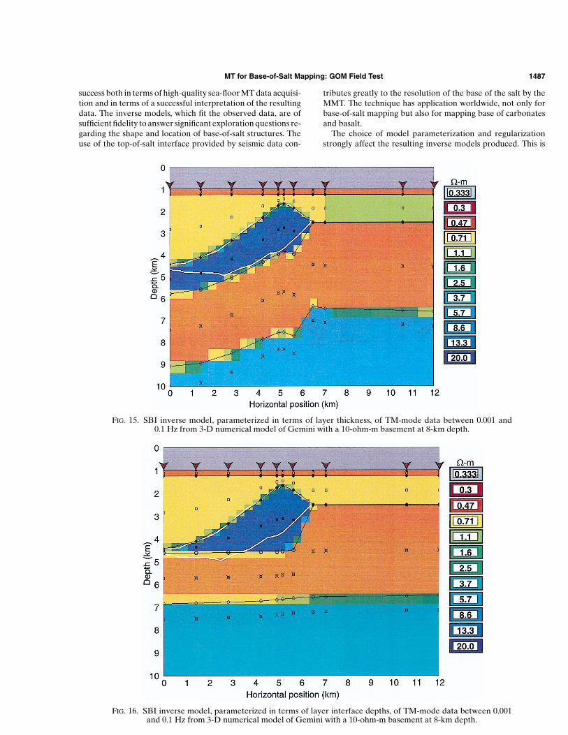
In order to demonstrate the effects of the choice of regular-ization on the final model, we used the 3-D numerical modelfrom the experiment design (salt structure shown in Figure 3,data shown in Figure 4) and added a resistive basement at adepth of 8 km. The numerical data between 0.001 and 0.1 Hzwas used in SBI inversions where the starting model was iden-tical to that used in Figure 12. Only the lower frequencies wereused since the object is to illustrate the effects on the baseof salt and deep resistive structure. Two SBI inversions wererun, one parameterized by layer thickness and the other pa-rameterized by layer interface depth. In the second case, theregularization favors models with a layer boundary of smooth(constant) depth. Both inversions assumed 5% noise and wererun to a rms data misfit of 1.0. Figures 15 and 16 show the final


FIG. 8. Polar impedance diagrams for the nine seafloor sites, Sites are ordered from southwest (site 5) to northeast(site 19). Rows are constant frequency in hertz (high frequency at top, low frequency at bottom), and columnsare constant site location. North is up, east is to the right.

FIG. 9. RRI TM-mode inversion. Starting model was 0.7-ohm-m half-space. White line shows salt outline asinterpreted from 3-D prestack depth-migrated seismic data. Seawater was not included in the inversion model.Sea-floor MT sites shown by red triangles.


inverse models for the thickness and depth parameterizations,respectively.

The resemblance between Figure 12 the field data inversion,and Figure 15, the numerical model data inversion, is striking.

FIG. 10. NLCG TM-mode inversion. Starting model was 0.7-ohm-m half-space. White line shows salt outline asinterpreted from 3-D prestack depth-migrated seismic data. Sea-floor MT sites shown by red triangles.

FIG. 11. Occam 2-D TM-mode inversion. Starting model was 0.7-ohm-m half-space. White line shows salt outlineas interpreted from 3-D prestack depth-migrated seismic data. No smoothing across blocks at top of salt. Sea-floorMT sites shown by red triangles.

The thickness of salt in the inverse model at the beginning ofthe line where the salt is deep is due to the thickness param-eterization. Comparing Figures 15 and 16, we see that if themodel is parameterized in depth, the salt is thinned to almost

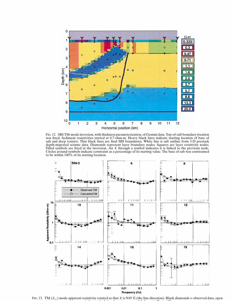
FIG. 12. SBI TM-mode inversion, with thickness parameterization, of Gemini data. Top-of-salt boundary locationwas fixed. Sediment resistivities started at 0.7-ohm-m. Heavy black lines indicate starting location of base ofsalt and deep resistor. Thin black lines are final SBI boundaries. White line is salt outline from 3-D prestackdepth-migrated seismic data. Diamonds represent layer boundary nodes. Squares are layer resistivity nodes.Filled symbols are fixed in the inversion. An X through a symbol indicates it is linked to the previous node.Circles around symbols indicate constraint as a percentage of its starting value. The base of salt was constrainedto be within 100% of its starting location.

FIG. 13. TM (Zxy) mode apparent resistivity rotated so that X is N45◦E (the line direction). Black diamonds = observed data, opencircles calculation from in erse model sho n in Figure 12


zero. The effect on the deep resistor is also significant. Whilethe deep resistor is flat at a depth of 8 km, the thickness in-version has produced roughly 2 km of relief on this interfaceby keeping the thickness of the overlying sediments roughlyconstant.

Using only the SBI inverse in isolation, one could not choosebetween the two possible SBI models. However, when the twoSBI models are compared to the smooth inverse models (par-ticularly the Occam 2-D model that incorporated a sharp con-trast at the top of salt), the SBI thickness model can be selectedas the preferred interpretation since it is more consistent withthe smooth models. The SBI depth model can be taken as awarning that the salt thickness at the beginning of the line,where it is deepest, can be anywhere between zero and 1 km.

SENSITIVITY OF MMT DATA TO VARIATIONSIN BASE-OF-SALT DEPTH

As we have seen from comparing the depth and thickness in-versions of the 3-D numerical data, two models with significantdifferences can be found which both fit the data equally well.In the case of the thickness parameterization (Figure 15), themaximum error in the base of salt is at the beginning of the line,where the salt is thinnest, and is about 1 km at a depth of 5 km,or 20%. In the case of the depth parameterization (Figure 16),the maximum error in the base salt occurs below the crest of the

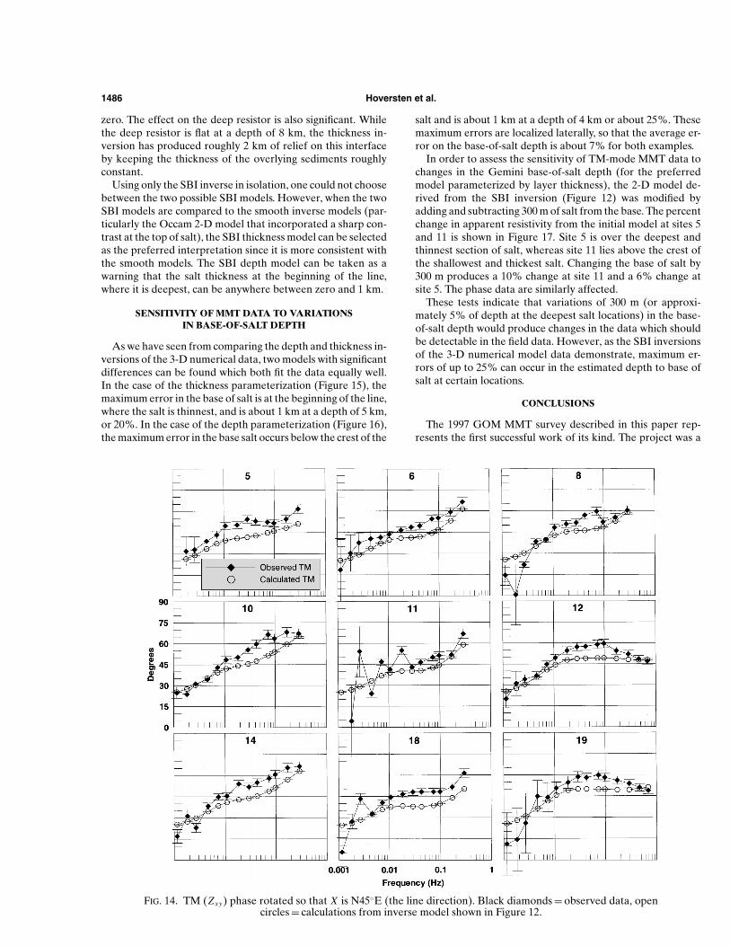
FIG. 14. TM (Zxy) phase rotated so that X is N45◦E (the line direction). Black diamonds = observed data, opencircles = calculations from inverse model shown in Figure 12.

salt and is about 1 km at a depth of 4 km or about 25%. Thesemaximum errors are localized laterally, so that the average er-ror on the base-of-salt depth is about 7% for both examples.

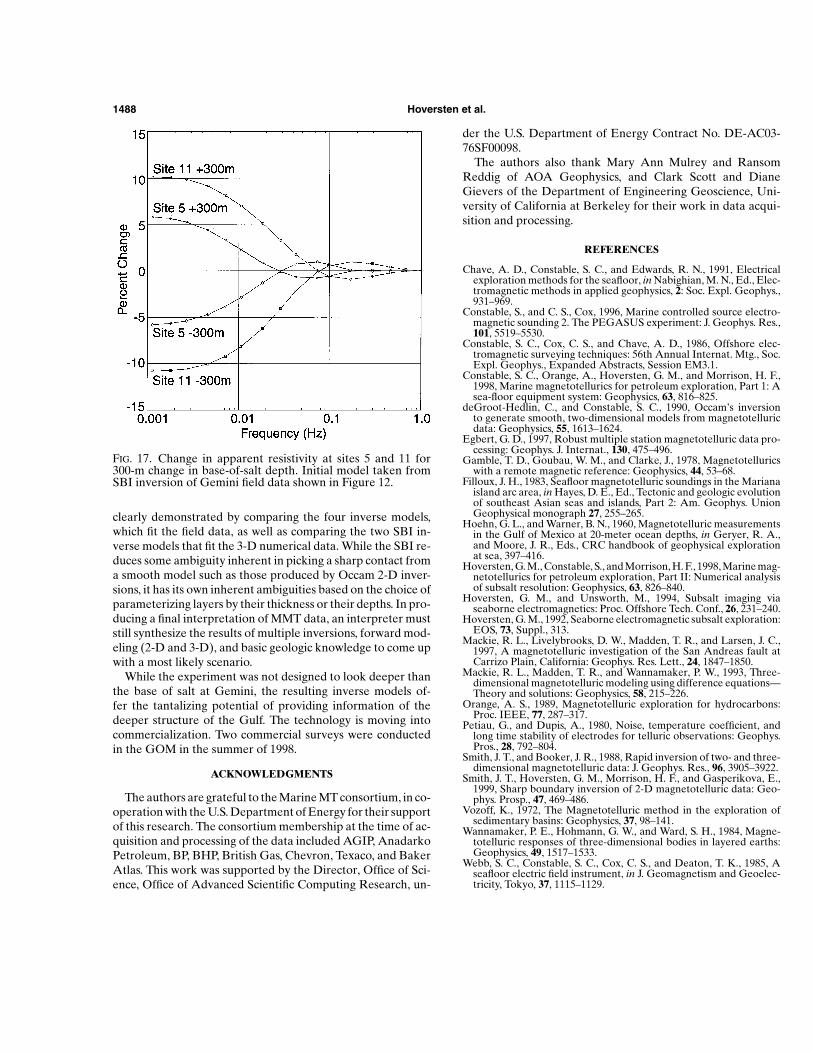
In order to assess the sensitivity of TM-mode MMT data tochanges in the Gemini base-of-salt depth (for the preferredmodel parameterized by layer thickness), the 2-D model de-rived from the SBI inversion (Figure 12) was modified byadding and subtracting 300 m of salt from the base. The percentchange in apparent resistivity from the initial model at sites 5and 11 is shown in Figure 17. Site 5 is over the deepest andthinnest section of salt, whereas site 11 lies above the crest ofthe shallowest and thickest salt. Changing the base of salt by300 m produces a 10% change at site 11 and a 6% change atsite 5. The phase data are similarly affected.

These tests indicate that variations of 300 m (or approxi-mately 5% of depth at the deepest salt locations) in the base-of-salt depth would produce changes in the data which shouldbe detectable in the field data. However, as the SBI inversionsof the 3-D numerical model data demonstrate, maximum er-rors of up to 25% can occur in the estimated depth to base ofsalt at certain locations.

CONCLUSIONS

The 1997 GOM MMT survey described in this paper rep-resents the first successful work of its kind. The project was a


success both in terms of high-quality sea-floor MT data acquisi-tion and in terms of a successful interpretation of the resultingdata. The inverse models, which fit the observed data, are ofsufficient fidelity to answer significant exploration questions re-garding the shape and location of base-of-salt structures. Theuse of the top-of-salt interface provided by seismic data con-

FIG. 15. SBI inverse model, parameterized in terms of layer thickness, of TM-mode data between 0.001 and0.1 Hz from 3-D numerical model of Gemini with a 10-ohm-m basement at 8-km depth.

FIG. 16. SBI inverse model, parameterized in terms of layer interface depths, of TM-mode data between 0.001and 0.1 Hz from 3-D numerical model of Gemini with a 10-ohm-m basement at 8-km depth.

tributes greatly to the resolution of the base of the salt by theMMT. The technique has application worldwide, not only forbase-of-salt mapping but also for mapping base of carbonatesand basalt.

The choice of model parameterization and regularizationstrongly affect the resulting inverse models produced. This is


FIG. 17. Change in apparent resistivity at sites 5 and 11 for300-m change in base-of-salt depth. Initial model taken fromSBI inversion of Gemini field data shown in Figure 12.

clearly demonstrated by comparing the four inverse models,which fit the field data, as well as comparing the two SBI in-verse models that fit the 3-D numerical data. While the SBI re-duces some ambiguity inherent in picking a sharp contact froma smooth model such as those produced by Occam 2-D inver-sions, it has its own inherent ambiguities based on the choice ofparameterizing layers by their thickness or their depths. In pro-ducing a final interpretation of MMT data, an interpreter muststill synthesize the results of multiple inversions, forward mod-eling (2-D and 3-D), and basic geologic knowledge to come upwith a most likely scenario.

While the experiment was not designed to look deeper thanthe base of salt at Gemini, the resulting inverse models of-fer the tantalizing potential of providing information of thedeeper structure of the Gulf. The technology is moving intocommercialization. Two commercial surveys were conductedin the GOM in the summer of 1998.

ACKNOWLEDGMENTS

The authors are grateful to the Marine MT consortium, in co-operation with the U.S. Department of Energy for their supportof this research. The consortium membership at the time of ac-quisition and processing of the data included AGIP, AnadarkoPetroleum, BP, BHP, British Gas, Chevron, Texaco, and BakerAtlas. This work was supported by the Director, Office of Sci-ence, Office of Advanced Scientific Computing Research, un-

der the U.S. Department of Energy Contract No. DE-AC03-76SF00098.

The authors also thank Mary Ann Mulrey and RansomReddig of AOA Geophysics, and Clark Scott and DianeGievers of the Department of Engineering Geoscience, Uni-versity of California at Berkeley for their work in data acqui-sition and processing.

REFERENCES

Chave, A. D., Constable, S. C., and Edwards, R. N., 1991, Electricalexploration methods for the seafloor, in Nabighian, M. N., Ed., Elec-tromagnetic methods in applied geophysics, 2: Soc. Expl. Geophys.,931–969.

Constable, S., and C. S., Cox, 1996, Marine controlled source electro-magnetic sounding 2. The PEGASUS experiment: J. Geophys. Res.,101, 5519–5530.

Constable, S. C., Cox, C. S., and Chave, A. D., 1986, Offshore elec-tromagnetic surveying techniques: 56th Annual Internat. Mtg., Soc.Expl. Geophys., Expanded Abstracts, Session EM3.1.

Constable, S. C., Orange, A., Hoversten, G. M., and Morrison, H. F.,1998, Marine magnetotellurics for petroleum exploration, Part 1: Asea-floor equipment system: Geophysics, 63, 816–825.

deGroot-Hedlin, C., and Constable, S. C., 1990, Occam’s inversionto generate smooth, two-dimensional models from magnetotelluricdata: Geophysics, 55, 1613–1624.

Egbert, G. D., 1997, Robust multiple station magnetotelluric data pro-cessing: Geophys. J. Internat., 130, 475–496.

Gamble, T. D., Goubau, W. M., and Clarke, J., 1978, Magnetotelluricswith a remote magnetic reference: Geophysics, 44, 53–68.

Filloux, J. H., 1983, Seafloor magnetotelluric soundings in the Marianaisland arc area, in Hayes, D. E., Ed., Tectonic and geologic evolutionof southeast Asian seas and islands, Part 2: Am. Geophys. UnionGeophysical monograph 27, 255–265.

Hoehn, G. L., and Warner, B. N., 1960, Magnetotelluric measurementsin the Gulf of Mexico at 20-meter ocean depths, in Geryer, R. A.,and Moore, J. R., Eds., CRC handbook of geophysical explorationat sea, 397–416.

Hoversten, G. M., Constable, S., and Morrison, H. F., 1998, Marine mag-netotellurics for petroleum exploration, Part II: Numerical analysisof subsalt resolution: Geophysics, 63, 826–840.

Hoversten, G. M., and Unsworth, M., 1994, Subsalt imaging viaseaborne electromagnetics: Proc. Offshore Tech. Conf., 26, 231–240.

Hoversten, G. M., 1992, Seaborne electromagnetic subsalt exploration:EOS, 73, Suppl., 313.

Mackie, R. L., Livelybrooks, D. W., Madden, T. R., and Larsen, J. C.,1997, A magnetotelluric investigation of the San Andreas fault atCarrizo Plain, California: Geophys. Res. Lett., 24, 1847–1850.

Mackie, R. L., Madden, T. R., and Wannamaker, P. W., 1993, Three-dimensional magnetotelluric modeling using difference equations—Theory and solutions: Geophysics, 58, 215–226.

Orange, A. S., 1989, Magnetotelluric exploration for hydrocarbons:Proc. IEEE, 77, 287–317.

Petiau, G., and Dupis, A., 1980, Noise, temperature coefficient, andlong time stability of electrodes for telluric observations: Geophys.Pros., 28, 792–804.

Smith, J. T., and Booker, J. R., 1988, Rapid inversion of two- and three-dimensional magnetotelluric data: J. Geophys. Res., 96, 3905–3922.

Smith, J. T., Hoversten, G. M., Morrison, H. F., and Gasperikova, E.,1999, Sharp boundary inversion of 2-D magnetotelluric data: Geo-phys. Prosp., 47, 469–486.

Vozoff, K., 1972, The Magnetotelluric method in the exploration ofsedimentary basins: Geophysics, 37, 98–141.

Wannamaker, P. E., Hohmann, G. W., and Ward, S. H., 1984, Magne-totelluric responses of three-dimensional bodies in layered earths:Geophysics, 49, 1517–1533.

Webb, S. C., Constable, S. C., Cox, C. S., and Deaton, T. K., 1985, Aseafloor electric field instrument, in J. Geomagnetism and Geoelec-tricity, Tokyo, 37, 1115–1129.

Documents

Marine magnetotellurics for base-of-salt mapping: Gulf of