Maritime Radio Propagation with the Effects of Ship Motions · To further investigate the maritime radio propagation with the effects of ship motions, ... establishes a radio propagation

Maritime Radio Propagation with the Effects of Ship

Motions

Fang Huang, Yong Bai, and Wencai Du College of Information Science and Technology, Hainan University, Haikou, 570228, China

Email: [email protected]; [email protected]; [email protected]

Abstract—For designing maritime wireless transmission

system, the radio propagation over sea surface needs to be

known first. One of the distinct characteristics of maritime radio

propagation is the impact of ship motions due to the fluctuation

of sea waves. This paper establishes a radio propagation model

with the integration of the effects of ship motions. Using such

an integrated radio propagation model, the maritime radio

propagation characteristics are analyzed and discussed under

different transmission distances, different carrier frequencies,

and different motion types. Index Terms—Radio propagation, Maritime communications,

Channel modeling

I. INTRODUCTION

In the ship-to-ship and the ship-to-shore wireless

communications over the sea, the radio signal propagates

over the sea surface. Hence, the radio propagation over

sea surface needs to be studied first for designing the

maritime wireless transmission system. One of the

distinct characteristics of maritime radio propagation is

the impact of ship motions due to the fluctuation of sea

waves. The angle between the transmit antenna and the

receive antenna changes with ship motions, which results

in the fluctuations of the received power at the receive

antenna. In previous investigations on maritime radio

propagation models, several deterministic models such as

the Free Space Loss (FSL) model and the Plain Earth

Loss (PEL) model based on Friis transmission formula

and two-ray tracing method have been commonly used as

references for the open-sea environment [1]-[4]. In

addition, the distance between the transmitter and the

receiver can be far in the maritime radio transmission

environment, and the effect of the earth curvature cannot

be ignored. Another deterministic path-loss model for the

open-sea environment was proposed in accordance with

measurements at 2 GHz with a maximum distance of 45

km [5]-[7]

effects including effective reflection, divergence, and

diffraction due to rough sea and earth curvature. However,

the abovementioned studies have not considered the

effects of ship motions. Hubert et al. presented a maritime

radio link channel simulator and studied the impact of

Manuscript received January 12, 2015; revised May 13, 2015. Corresponding author: Wencai Du, email: [email protected]

doi:10.12720/jcm.10.5.345-351

ship motions with a 3D antenna gain model [8]. Therein,

the numerical results of the receive power was given only

for the up-down ship motion at 2.4GHz carrier frequency

with a fixed transmission distance. Nevertheless, it still

lacks the study of maritime radio propagation with the

effects of ship motions under different transmission

distances, different carrier frequencies, and different

motion types. To further investigate the maritime radio

propagation with the effects of ship motions, this paper

first improves the traditional two-ray propagation model

by taking into account the earth curvature, and then

establishes a radio propagation model by integrating the

3D antenna gain model of ship motions with the

improved two-ray propagation model. Using such a

model, the maritime radio propagation characteristics are

analyzed and discussed under different transmission

distances, carrier frequencies, and different motion types.

The rest of this paper is organized as follows. Section

II describes the maritime radio propagation path. Section

III improves traditional two-ray propagation model by

taking into account the earth curvature. Section IV

establishes the radio propagation model by integrating a

3D model antenna direction gain model of ship motions

with the improved two-ray propagation model. Section V

presents the numerical results of the radio propagation

with the effects of ship motions using the established

model. Section VI concludes this paper.

II. MARITIME RADIO PROPAGATION PATH

Frist, we discuss the radio propagation path over sea

surface. For over-the-sea transmission to and from ships,

the effect of earth curvature on the radio propagation

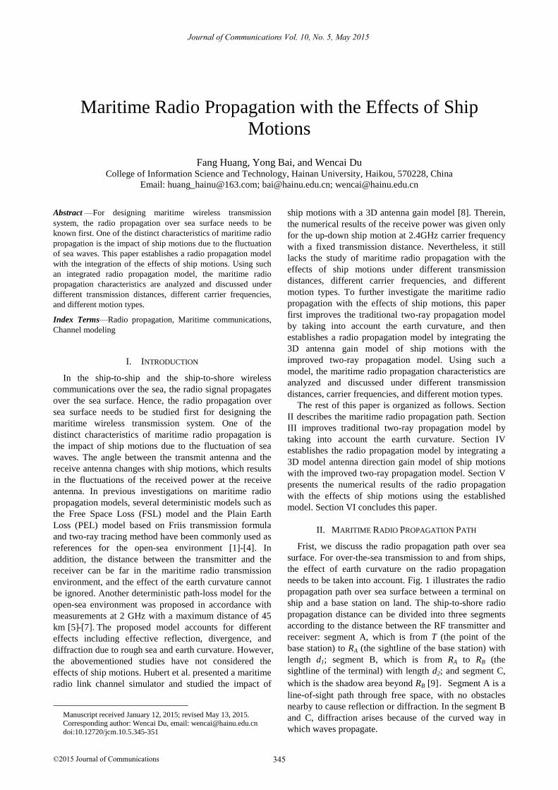
needs to be taken into account. Fig. 1 illustrates the radio

propagation path over sea surface between a terminal on

ship and a base station on land. The ship-to-shore radio

propagation distance can be divided into three segments

according to the distance between the RF transmitter and

receiver: segment A, which is from T (the point of the

base station) to RA (the sightline of the base station) with

length d1; segment B, which is from RA to RB (the

sightline of the terminal) with length d2; and segment C,

which is the shadow area beyond RB [9]．Segment A is a

line-of-sight path through free space, with no obstacles

nearby to cause reflection or diffraction. In the segment B

and C, diffraction arises because of the curved way in

which waves propagate.

Journal of Communications Vol. 10, No. 5, May 2015

345©2015 Journal of Communications

. The proposed model accounts for different

d1 d2

d3

RA RB

RC

A B

C

Ht

Hr

Hr

T

Re

Fig. 1. Three distance segments of maritime radio propagation

Assume that the antenna heights of base station and

terminal are Ht, and Hr, respectively. Using trigonometry,

it can be calculated that [10]

2 2 2

1 ( )e t ed R H R

(1)

2

1 2 e t td R H H

(2)

where Re is the earth radius, and Re=8500km. Because

e tR H , we can get

1 2 e td R H

(3)

Similarly,

2 2 e rd R H

(4)

III. IMPROVED TWO

The reflection effect from the sea surface and the

scattering effect due to the roughness of sea waves result

in multipath components of the transmitted signal at the

receive antenna. The random phase and amplitudes of

different multipath components cause fluctuations in

signal strength [11]. In [12], the roughness factor

judgment, Rayleigh judgment, coherent reflection

coefficient method and specular and diffuse reflection

coefficients method are used to analyze the reflection

characteristics of electromagnetic waves over the sea. It is

concluded that the sea surface can be assumed smooth

mirror surface when the sea state is seven and the grazing

angle is from 0 to 1.3 degrees, or the sea state is six and

the grazing angle is from 0 to 2.5 degrees. This paper

assumes that the sea surface is calm, and only considers

the effect of specular reflection. Thus, a two-ray model

can be used for analyzing the radio propagation over sea

surface. As shown in Fig. 2, a two-ray model of radio

propagation includes a direct path and a specular

reflection path. The direct signal path is the line of sight

(LOS) signal propagation between the transmitter and the

receiver. The specular reflection path is produced by the

reflection from the smooth sea surface [13].

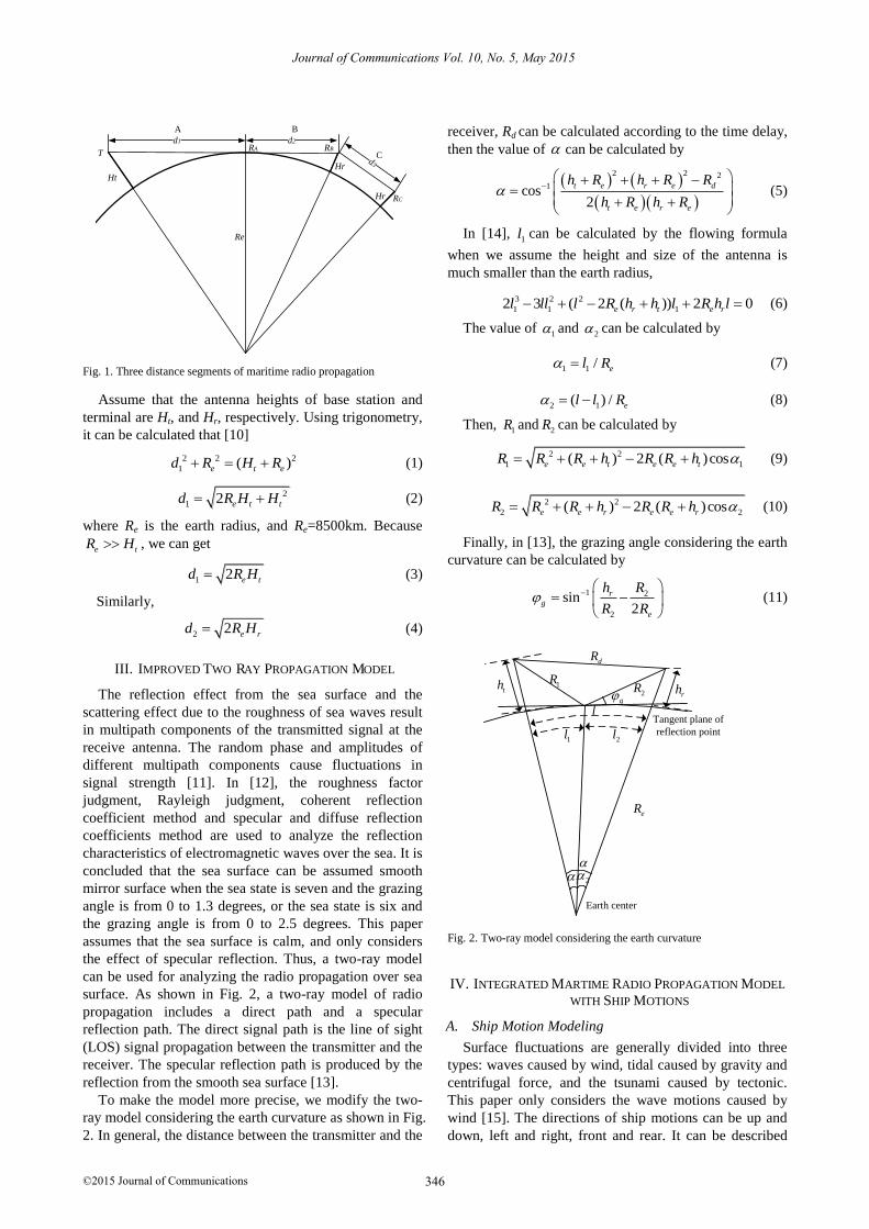
To make the model more precise, we modify the two-

ray model considering the earth curvature as shown in Fig.

2. In general, the distance between the transmitter and the

receiver, Rd can be calculated according to the time delay,

then the value of can be calculated by

2 2 2

1cos2

t e r e d

t e r e

h R h R R

h R h R

(5)

In [14], 1l can be calculated by the flowing formula

when we assume the height and size of the antenna is

much smaller than the earth radius,

3 2 2

1 1 12 3 ( 2 ( )) 2 0e r t e rl ll l R h h l R h l

(6)

The value of 1 and

2 can be calculated by

1 1 / el R

(7)

2 1( ) / el l R

(8)

Then, 1R and

2R can be calculated by

2 2

1 1( ) 2 ( )cose e t e e tR R R h R R h

(9)

2 2

2 2( ) 2 ( )cose e r e e rR R R h R R h

(10)

Finally, in [13], the grazing angle considering the earth

curvature can be calculated by

1 2

2

sin2

r

g

e

h R

R R

(11)

2

rhth

dR

1R2R

l

1l 2l

1

Earth center

Tangent plane of

reflection point

g

eR

Fig. 2. Two-ray model considering the earth curvature

IV. INTEGRATED MARTIME RADIO PROPAGATION MODEL

WITH SHIP MOTIONS

A. Ship Motion Modeling

Surface fluctuations are generally divided into three

types: waves caused by wind, tidal caused by gravity and

centrifugal force, and the tsunami caused by tectonic.

This paper only considers the wave motions caused by

wind [15]. The directions of ship motions can be up and

down, left and right, front and rear. It can be described



AY ROPAGATION ODELR P M

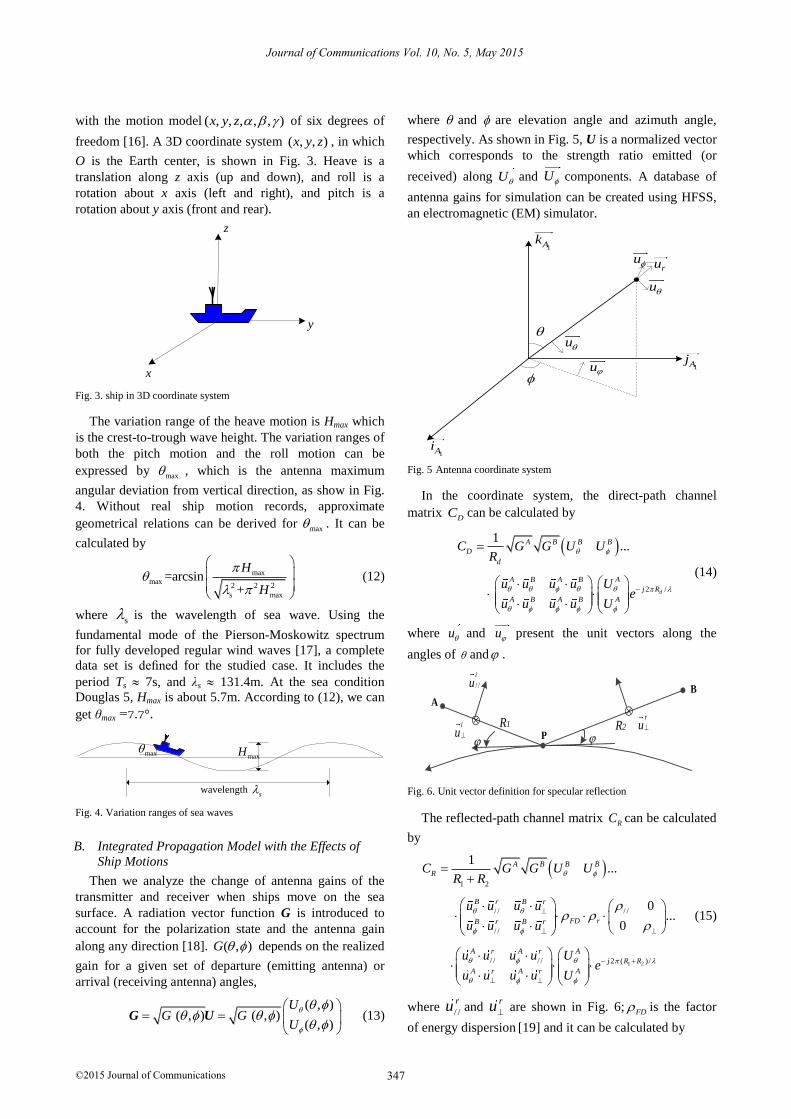
with the motion model ( , , , , , )x y z of six degrees of

freedom [16]. A 3D coordinate system ( , , )x y z , in which

O is the Earth center, is shown in Fig. 3. Heave is a

translation along z axis (up and down), and roll is a

rotation about x axis (left and right), and pitch is a

rotation about y axis (front and rear).

x

z

y

Fig. 3. ship in 3D coordinate system

The variation range of the heave motion is Hmax which

is the crest-to-trough wave height. The variation ranges of

both the pitch motion and the roll motion can be

expressed by max , which is the antenna maximum

angular deviation from vertical direction, as show in Fig.

4. Without real ship motion records, approximate

geometrical relations can be derived for max . It can be

calculated by

max

max2 2 2

s max

=arcsin+

H

H

(12)

where s is the wavelength of sea wave. Using the

fundamental mode of the Pierson-Moskowitz spectrum

for fully developed regular wind waves [17], a complete

data set is defined for the studied case. It includes the

period Ts 7s, and λs 131.4m. At the sea condition

Douglas 5, Hmax is about 5.7m. According to (12), we can

get θmax =7.7°.

maxmaxH

wavelengths

Fig. 4. Variation ranges of sea waves

B. Integrated Propagation Model with the Effects of

Ship Motions

Then we analyze the change of antenna gains of the

transmitter and receiver when ships move on the sea

surface. A radiation vector function G is introduced to

account for the polarization state and the antenna gain

along any direction [18]. ( , )G depends on the realized

gain for a given set of departure (emitting antenna) or

arrival (receiving antenna) angles,

( , )( , ) ( , )

( , )

UG G

U

G U

(13)

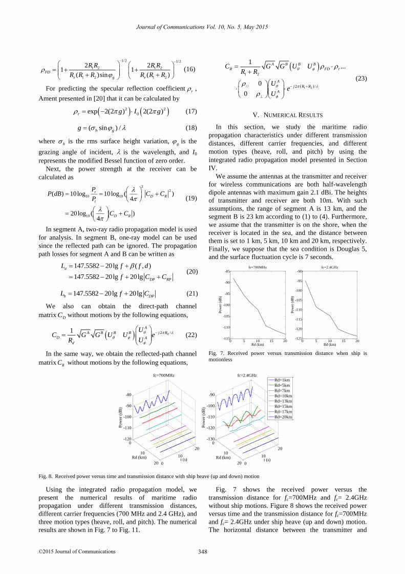
where and are elevation angle and azimuth angle,

respectively. As shown in Fig. 5, U is a normalized vector

which corresponds to the strength ratio emitted (or

received) along U and U components. A database of

antenna gains for simulation can be created using HFSS,

an electromagnetic (EM) simulator.

u

u

ruu

u

1Ai

1Aj

1Ak

Fig. 5 Antenna coordinate system

In the coordinate system, the direct-path channel

matrix DC can be calculated by

2 /

1...

d

A B B B

D

d

A B A B A

j R

A B A B A

C G G U UR

u u u u Ue

u u u u U

(14)

where u and u present the unit vectors along the

angles of and .

A

B

PR1 R2

r

ui

u

/ /

i

u

Fig. 6. Unit vector definition for specular reflection

The reflected-path channel matrix RC can be calculated

by

1 2

1 2

/ // /

/ /

/ / / / 2 ( )/

1...

0...

0

A B B B

R

B r B r

FD rB r B r

A r A r A

j R R

A r A r A

C G G U UR R

u u u u

u u u u

u u u u Ue

u u u u U

(15)

where / /

ru and ru are shown in Fig. 6;

FD is the factor

of energy dispersion [19] and it can be calculated by



1/2 1/2

1 2 1 2

1 2 1 2

2 21 1

( )sin ( )FD

e g e

R R R R

R R R R R R

(16)

For predicting the specular reflection coefficientr ,

Ament presented in [20] that it can be calculated by

2 2

0exp 2(2 ) 2(2 )r g I g

(17)

( sin ) /h gg

(18)

where h is the rms surface height variation,

g is the

grazing angle of incident, is the wavelength, and I0

represents the modified Bessel function of zero order.

Next, the power strength at the receiver can be

calculated as 2

2

10 10

10

( ) 10log 10log ( )4

20log ( )4

r

D R

t

D R

PP dB C C

P

C C

(19)

In segment A, two-ray radio propagation model is used

for analysis. In segment B, one-ray model can be used

since the reflected path can be ignored. The propagation

path losses for segment A and B can be written as

147.5582 20lg ( , )

147.5582 20lg 20lg

a

DP RP

L f f d

f C C

(20)

147.5582 20lg 20lgb DPL f C (21)

We also can obtain the direct-path channel

matrixDC without motions by the following equations,

2 /1d

A

j RA B B B

D A

d

UC G G U U e

UR

(22)

In the same way, we obtain the reflected-path channel

matrixRC without motions by the following equations,

1 2

1 2

/ / 2 ( )/

1...

0

0

A B B B

R FD r

A

j R R

A

C G G U UR R

Ue

U

(23)

V. NUMERICAL RESULTS

In this section, we study the maritime radio

propagation characteristics under different transmission

distances, different carrier frequencies, and different

motion types (heave, roll, and pitch) by using the

integrated radio propagation model presented in Section

IV.

We assume the antennas at the transmitter and receiver

for wireless communications are both half-wavelength

dipole antennas with maximum gain 2.1 dBi. The heights

of transmitter and receiver are both 10m. With such

assumptions, the range of segment A is 13 km, and the

segment B is 23 km according to (1) to (4). Furthermore,

we assume that the transmitter is on the shore, when the

receiver is located in the sea, and the distance between

them is set to 1 km, 5 km, 10 km and 20 km, respectively.

Finally, we suppose that the sea condition is Douglas 5,

and the surface fluctuation cycle is 7 seconds.

0 5 10 15 20-125

-120

-115

-110

-105

-100

-95

-90fc=2.4GHz

Rd (km)

Po

wer

(d

B)

0 5 10 15 20-115

-110

-105

-100

-95

-90

-85fc=700MHz

Rd (km)

Po

wer

(d

B)

Fig. 7. Received power versus transmission distance when ship is

motionless

0

10

20

0

10

20

-130

-120

-110

-100

-90

t (s)

fc=2.4GHz

Rd (km)

Po

wer

(dB

)

0

10

20

0

10

20

-120

-110

-100

-90

-80

t (s)

fc=700MHz

Rd (km)

Po

wer

(dB

)

Rd=1km

Rd=5km

Rd=7km

Rd=10km

Rd=13km

Rd=15km

Rd=17km

Rd=20km

Fig. 8. Received power versus time and transmission distance with ship heave (up and down) motion

Using the integrated radio propagation model, we

present the numerical results of maritime radio

propagation under different transmission distances,

different carrier frequencies (700 MHz and 2.4 GHz), and

three motion types (heave, roll, and pitch). The numerical

results are shown in Fig. 7 to Fig. 11.

Fig. 7 shows the received power versus the

transmission distance for fc=700MHz and fc= 2.4GHz

without ship motions. Figure 8 shows the received power

versus time and the transmission distance for fc=700MHz

and fc= 2.4GHz under ship heave (up and down) motion.

The horizontal distance between the transmitter and



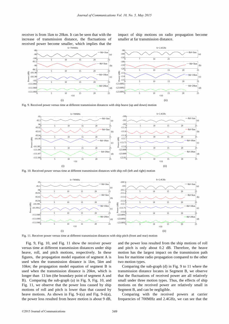
receiver is from 1km to 20km. It can be seen that with the

increase of transmission distance, the fluctuations of

received power become smaller, which implies that the

impact of ship motions on radio propagation become

smaller at far transmission distance.

0 5 10 15 20 25-100

-90

-80

fc=700MHz

Rd=1km

0 5 10 15 20 25-96.5

-96

-95.5

Rd=5km

0 5 10 15 20 25-102

-101.99

-101.98

Po

wer

(dB

)

Rd=10km

0 5 10 15 20 25-113.1069

-113.1069

-113.1069

t (s)

Rd=20km

(a)

(b)

(c)

(d)

0 7 14 21-110

-100

-90

fc=2.4GHz

Rd=1km

0 5 10 15 20 25-120

-110

-100

Rd=5km

0 5 10 15 20 25-115

-114

-113

Po

wer

(dB

)

Rd=10km

0 5 10 15 20 25-123.8092

-123.8092

-123.8092

t (s)

Rd=20km

(a)

(b)

(c)

(d)

(i) (ii)

Fig. 9. Received power versus time at different transmission distances with ship heave (up and down) motion

0 5 10 15 20 25-96

-95.5

-95

fc=700MHz

Rd=1km

0 5 10 15 20 25-95.94

-95.93

-95.92

Rd=5km

0 5 10 15 20 25-101.995

-101.99

Po

wer

(dB

)

Rd=10km

0 5 10 15 20 25-113.108

-113.107

-113.106

t (s)

Rd=20km

(a)

(b)

(c)

(d)

0 5 10 15 20 25-102

-101

-100

fc=2.4GHz

Rd=1km

0 5 10 15 20 25-111.8

-111.6

-111.4

Rd=5km

0 5 10 15 20 25-113.8

-113.75

-113.7

Po

wer

(dB

)

Rd=10km

0 5 10 15 20 25-123.81

-123.809

-123.808

t (s)

Rd=20km

(a)

(b)

(c)

(d)

(i) (ii)

Fig. 10. Received power versus time at different transmission distances with ship roll (left and right) motion

0 5 10 15 20 25-96

-95.5

-95

fc=700MHz

Rd=1km

0 5 10 15 20 25-95.94

-95.93

-95.92

Rd=5km

0 5 10 15 20 25

-101.9912

-101.991

Po

wer

(dB

)

Rd=10km

0 5 10 15 20 25-113.1069

-113.1069

-113.1069

t (s)

Rd=20km

(a)

(b)

(c)

(d)

0 5 10 15 20 25-101.5

-101

-100.5

fc=2.4GHz

Rd=1km

0 5 10 15 20 25-111.8

-111.6

-111.4

Rd=5km

0 5 10 15 20 25-113.8

-113.75

-113.7

Po

wer

(dB

)

Rd=10km

0 5 10 15 20 25-123.8092

-123.8092

-123.8091

t (s)

Rd=20km

(a)

(b)

(c)

(d)

(i) (ii)

Fig. 11. Receiver power versus time at different transmission distances with ship pitch (front and rear) motion

Fig. 9, Fig. 10, and Fig. 11 show the receiver power

versus time at different transmission distances under ship

heave, roll, and pitch motions, respectively. In these

figures, the propagation model equation of segment A is

used when the transmission distance is 1km, 5km and

10km; the propagation model equation of segment B is

used when the transmission distance is 20km, which is

longer than 13 km (the boundary point of segment A and

B). Comparing the sub-graph (a) in Fig. 9, Fig. 10, and

Fig. 11, we observe that the power loss caused by ship

motions of roll and pitch is lower than that caused by

heave motions. As shown in Fig. 9-i(a) and Fig. 9-ii(a),

the power loss resulted from heave motion is about 9 dB,

and the power loss resulted from the ship motions of roll

and pitch is only about 0.2 dB. Therefore, the heave

motion has the largest impact on the transmission path

loss for maritime radio propagation compared to the other

two motion types.

Comparing the sub-graph (d) in Fig. 9 to 11 where the

transmission distance locates in Segment B, we observe

that the fluctuations of received power are all relatively

small under three motion types. Thus, the effects of ship

motions on the received power are relatively small in

Segment B, and can be negligible.

Comparing with the received powers at carrier

frequencies of 700MHz and 2.4GHz, we can see that the



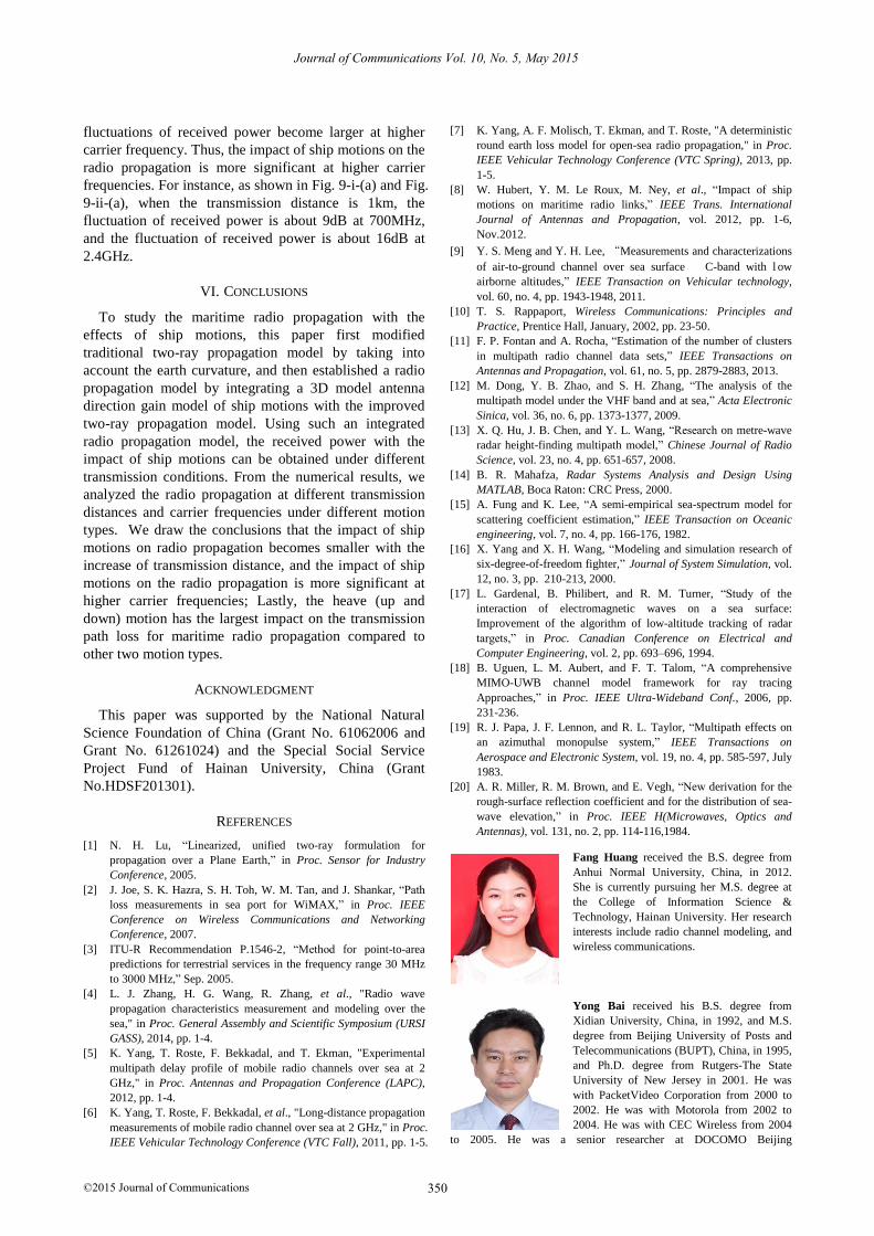
fluctuations of received power become larger at higher

carrier frequency. Thus, the impact of ship motions on the

radio propagation is more significant at higher carrier

frequencies. For instance, as shown in Fig. 9-i-(a) and Fig.

9-ii-(a), when the transmission distance is 1km, the

fluctuation of received power is about 9dB at 700MHz,

and the fluctuation of received power is about 16dB at

2.4GHz.

VI. CONCLUSIONS

To study the maritime radio propagation with the

effects of ship motions, this paper first modified

traditional two-ray propagation model by taking into

account the earth curvature, and then established a radio

propagation model by integrating a 3D model antenna

direction gain model of ship motions with the improved

two-ray propagation model. Using such an integrated

radio propagation model, the received power with the

impact of ship motions can be obtained under different

transmission conditions. From the numerical results, we

analyzed the radio propagation at different transmission

distances and carrier frequencies under different motion

types. We draw the conclusions that the impact of ship

motions on radio propagation becomes smaller with the

increase of transmission distance, and the impact of ship

motions on the radio propagation is more significant at

higher carrier frequencies; Lastly, the heave (up and

down) motion has the largest impact on the transmission

path loss for maritime radio propagation compared to

other two motion types.

ACKNOWLEDGMENT

This paper was supported by the National Natural

Science Foundation of China (Grant No. 61062006 and

Grant No. 61261024) and the Special Social Service

Project Fund of Hainan University, China (Grant

No.HDSF201301).

REFERENCES

[1] N. H. Lu, “Linearized, unified two-ray formulation for

propagation over a Plane Earth,” in Proc. Sensor for Industry

Conference, 2005.

[2] J. Joe, S. K. Hazra, S. H. Toh, W. M. Tan, and J. Shankar, “Path

loss measurements in sea port for WiMAX,” in Proc. IEEE

Conference on Wireless Communications and Networking

Conference, 2007.

[3] ITU-R Recommendation P.1546-2, “Method for point-to-area

predictions for terrestrial services in the frequency range 30 MHz

to 3000 MHz,” Sep. 2005.

[4] L. J. Zhang, H. G. Wang, R. Zhang, et al., "Radio wave

propagation characteristics measurement and modeling over the

sea," in Proc. General Assembly and Scientific Symposium (URSI

GASS), 2014, pp. 1-4.

[5] K. Yang, T. Roste, F. Bekkadal, and T. Ekman, "Experimental

multipath delay profile of mobile radio channels over sea at 2

GHz," in Proc. Antennas and Propagation Conference (LAPC),

2012, pp. 1-4.

[6] K. Yang, T. Roste, F. Bekkadal, et al., "Long-distance propagation

measurements of mobile radio channel over sea at 2 GHz," in Proc.

IEEE Vehicular Technology Conference (VTC Fall), 2011, pp. 1-5.

[7] K. Yang, A. F. Molisch, T. Ekman, and T. Roste, "A deterministic

round earth loss model for open-sea radio propagation," in Proc.

IEEE Vehicular Technology Conference (VTC Spring), 2013, pp.

1-5.

[8] W. Hubert, Y. M. Le Roux, M. Ney, et al., “Impact of ship

motions on maritime radio links,” IEEE Trans. International

Journal of Antennas and Propagation, vol. 2012, pp. 1-6,

Nov.2012.

[9] Y. S. Meng and Y. H. Lee, “Measurements and characterizations

of air-to-ground channel over sea surface C-band with l ow

airborne altitudes,” IEEE Transaction on Vehicular technology,

vol. 60, no. 4, pp. 1943-1948, 2011.

[10] T. S. Rappaport, Wireless Communications: Principles and

Practice, Prentice Hall, January, 2002, pp. 23-50.

[11] F. P. Fontan and A. Rocha, “Estimation of the number of clusters

in multipath radio channel data sets,” IEEE Transactions on

Antennas and Propagation, vol. 61, no. 5, pp. 2879-2883, 2013.

[12] M. Dong, Y. B. Zhao, and S. H. Zhang, “The analysis of the

multipath model under the VHF band and at sea,” Acta Electronic

Sinica, vol. 36, no. 6, pp. 1373-1377, 2009.

[13] X. Q. Hu, J. B. Chen, and Y. L. Wang, “Research on metre-wave

radar height-finding multipath model,” Chinese Journal of Radio

Science, vol. 23, no. 4, pp. 651-657, 2008.

[14] B. R. Mahafza, Radar Systems Analysis and Design Using

MATLAB, Boca Raton: CRC Press, 2000.

[15] A. Fung and K. Lee, “A semi-empirical sea-spectrum model for

scattering coefficient estimation,” IEEE Transaction on Oceanic

engineering, vol. 7, no. 4, pp. 166-176, 1982.

[16] X. Yang and X. H. Wang, “Modeling and simulation research of

six-degree-of-freedom fighter,” Journal of System Simulation, vol.

12, no. 3, pp. 210-213, 2000.

[17] L. Gardenal, B. Philibert, and R. M. Turner, “Study of the

interaction of electromagnetic waves on a sea surface:

Improvement of the algorithm of low-altitude tracking of radar

targets,” in Proc. Canadian Conference on Electrical and

Computer Engineering, vol. 2, pp. 693–696, 1994.

[18] B. Uguen, L. M. Aubert, and F. T. Talom, “A comprehensive

MIMO-UWB channel model framework for ray tracing

Approaches,” in Proc. IEEE Ultra-Wideband Conf., 2006, pp.

231-236.

[19] R. J. Papa, J. F. Lennon, and R. L. Taylor, “Multipath effects on

an azimuthal monopulse system,” IEEE Transactions on

Aerospace and Electronic System, vol. 19, no. 4, pp. 585-597, July

1983.

[20] A. R. Miller, R. M. Brown, and E. Vegh, “New derivation for the

rough-surface reflection coefficient and for the distribution of sea-

wave elevation,” in Proc. IEEE H(Microwaves, Optics and

Antennas), vol. 131, no. 2, pp. 114-116,1984.

Fang Huang received the B.S. degree from

Anhui Normal University, China, in 2012.

She is currently pursuing her M.S. degree at

the College of Information Science &

Technology, Hainan University. Her research

interests include radio channel modeling, and

wireless communications.

Yong Bai received his B.S. degree from

Xidian University, China, in 1992, and M.S.

degree from Beijing University of Posts and

Telecommunications (BUPT), China, in 1995,

and Ph.D. degree from Rutgers-The State

University of New Jersey in 2001. He was

with PacketVideo Corporation from 2000 to

2002. He was with Motorola from 2002 to

2004. He was with CEC Wireless from 2004

to 2005. He was a senior researcher at DOCOMO Beijing



Communication Labs from 2005 to 2009. He is a professor at College of

Information Science & Technology, Hainan University since 2010. He

acted as the Lead Guest Editor for EURASIP Journal on Wireless

Communications and Networking, Special Issue on Topology Control in

Wireless Ad Hoc and Sensor Networks. His current research interests

include mobile communications, and maritime communications. He is a

member of the IEEE.

Wencai Du received the B.S. degree from

Peking University, China, two M.S. Degrees

from ITC, The Netherlands, and Hohai

University, China, respectively, and Ph.D.

degree from South Australia University,

Australia. He was a Post-doctor Fellow in

Israel Institute of Technology (IIT), Haifa,

Israel. He is Dean of College of Information

Science & Technology at Hainan University

and Director of Maritime Communication and Engineering of Hainan

province. He has authored or coauthored 18 books and more than 80

scientific publications. He is currently members of the Editorial Board

of Inverts Journal of Science and Technology, India. He has taken

services on many professional conferences, including Conference Chair

of IEEE/ACIS ICIS 2011, Conference Co-Chair of IEEE/ACIS SNPD

2010, London, Conference Chair of IEEE/ACIS SERA 2009, and

Program Chair of IEEE/ACIS SNPD 2009, Daegu, Korea. His research

interests include several aspects of Information Technology and

Communication (ITC), including computer network and maritime

communications.



Documents

Maritime Radio Propagation with the Effects of Ship Motions · To further investigate the maritime radio propagation with the effects of ship motions, ... establishes a radio propagation