Mark Chaplain,The SIMBIOS Centre,Division of Mathematics,University of Dundee, Dundee, DD1 4HNSCOTLAND

Mathematical modelling of cell cytoskeleton biomechanics and cell membrane deformation

chaplain@maths.dundee.ac.uk

http://www.maths.dundee.ac.uk/~chaplain

http://www.simbios.ac.uk

Dr. Angélique Stéphanou,

Dr. Philippe Tracqui,

Laboratoire TIMC-IMAG,CNRS UMR 5525,Equipe Dynacell,38706 La Tronche CedexFrance

Collaborative work

“A mathematical model for the dynamics of large membranedeformations of isolated fibroblasts”Bull. Math. Biol. 66, 1119-1154 (2004)

Talk Overview

• Biological background• Examples of cell migration• Model derivation• Linear stability analysis• Numerical computations• Application to chemotaxis • Conclusions

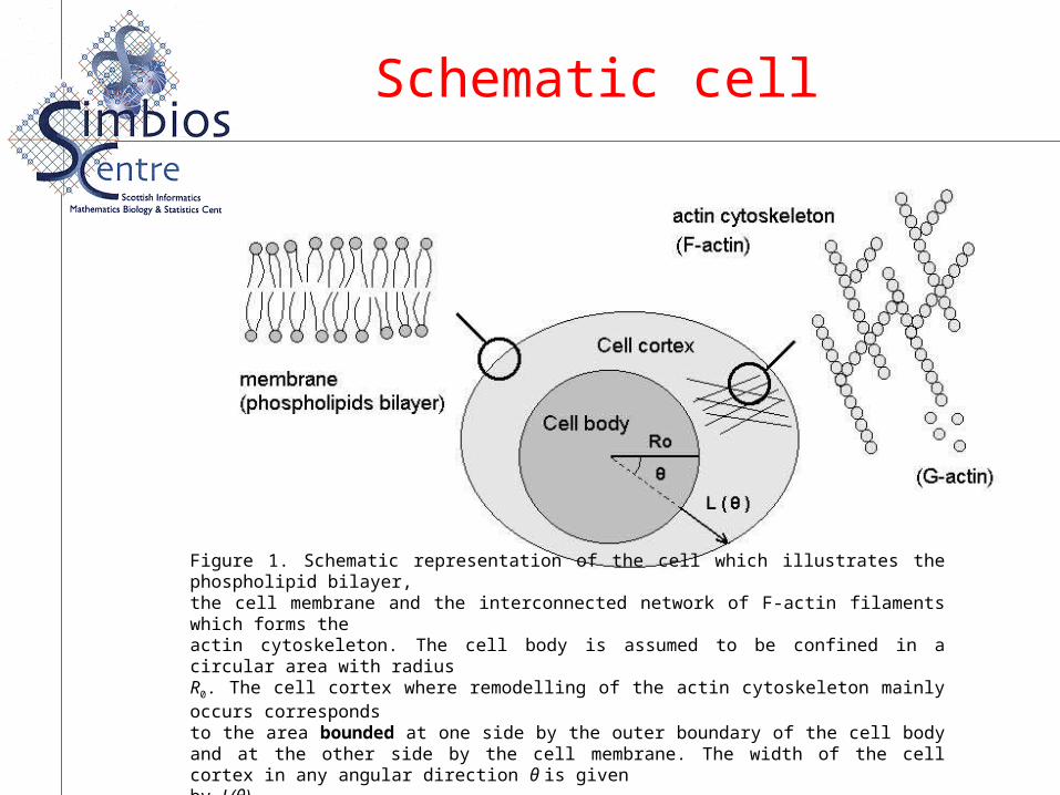
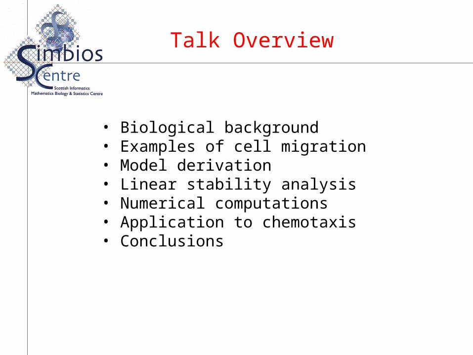
Figure 1. Schematic representation of the cell which illustrates the phospholipid bilayer,the cell membrane and the interconnected network of F-actin filaments which forms theactin cytoskeleton. The cell body is assumed to be confined in a circular area with radiusR0. The cell cortex where remodelling of the actin cytoskeleton mainly occurs correspondsto the area bounded at one side by the outer boundary of the cell body and at the other side by the cell membrane. The width of the cell cortex in any angular direction θ is givenby L(θ).

Schematic cell

Figure 2. Videomicrograph of non-migrating L929 fibroblasts observed with phase contrastmicroscopy. This videomicrograph shows the most typical morphologies exhibited bythis type of cell at their resting state (namely a non-migrating state). Fibroblasts typicallypresent ‘starry’ morphologies involving from 2 to 4 thin membrane extensions which aremore often homogeneously distributed around the cell body.

Figure 3. Spatio-temporal representations of the cells (cell polarity maps) which illustrates a variety of typical cell morphologies observed experimentally, with cells presenting, respectively, 2, 3 and 4 simultaneous protrusions each; the protrusive directions usually remain located along one axis for significantly long time periods (up to 12 h).

Aggregation of Dictyostelium amoebae towards a cAMP point source. Movie produced by G. Gerisch, Max-Planck-Institut fur Biochemie,

Martinsried, Germany.

A single cell moves chemotactically towards a cAMP point source.

Movie produced by G. Gerisch, Max-Planck-Institut fur Biochemie, Martinsried, Germany.

Cell migratory response to soluble chemicals:CHEMOTAXIS

No ECM

with ECM

ECM + tenascinEC &

Cell migratory response to local tissue environment cues

Non-diffusible molecules bound to the extracellular matrix

HAPTOTAXIS

Haptotaxis

Chemotaxis

Extracellular Matrix

TAF Receptor

Integrins

The Tissue Response Unit

Angiogenesis

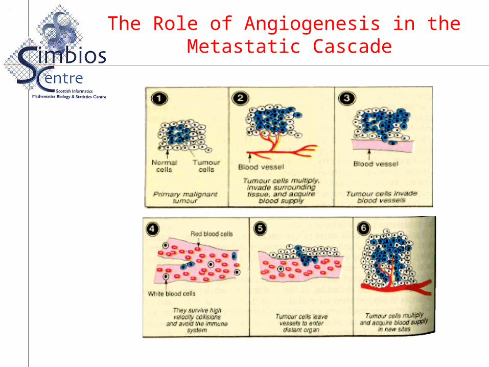
The Role of Angiogenesis in the Metastatic Cascade

Cell migration in wound healing

The Individual Cancer Cell“A Nonlinear Dynamical System”

Schematic representation of the cell which illustrates the phospholipid bilayer,the cell membrane and the interconnected network of F-actin filaments which forms theactin cytoskeleton. The cell body is assumed to be confined in a circular area with radiusR0. The cell cortex where remodelling of the actin cytoskeleton mainly occurs correspondsto the area bounded at one side by the outer boundary of the cell body and at the other side by the cell membrane. The width of the cell cortex in any angular direction θ is givenby L(θ).

Schematic cell

Modelling hypotheses

• Sol/gel transition of actin regulated by local calcium concentration

• Actin polymerisation in neighbourhood ofmembrane causes protrusion – Brownian ratchet mechanism

• Myosin I + actin = propulsion of filaments towards membrane

• Pressure-driven protrusion

Model Variables

Stress σ in the cytoskeleton - mechanical properties

F-actin concentration a – chemical dynamics of cytoskeleton

Membrane deformation L - linked to actin dynamics

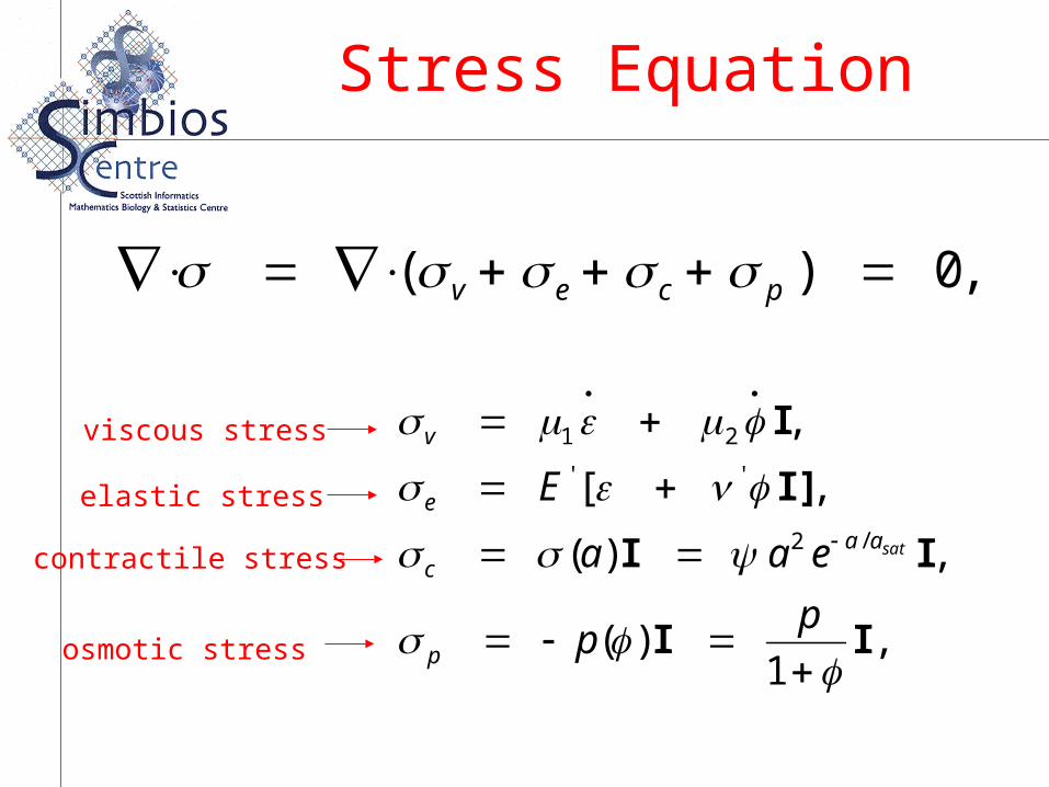
Stress Equation

,0)( pcev

,1

)(

,)(

[/2

''

21

II

II

]I

I

pp

eaa

E

p

aac

e

v

sat

,

,

contractile stress

osmotic stress

elastic stress

viscous stress

stress osmotic

network actomyosin of activity econtractil

ratio) Poisson'smodulus, Young's(

network actin of sviscositie bulk and shearand

dilation

tensor identity

directions tangential and radial in ntdisplaceme

tensor strain

1

)(

)(

)21/(),1/(

),2

1

''

2

p

a

E

EE

vu

T

u

I

(u

uu

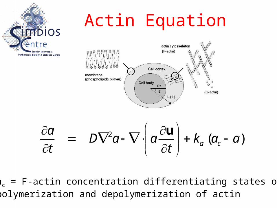
Actin Equation

).(2 aakt

aaDt

aca

u

ac = F-actin concentration differentiating states of polymerization and depolymerization of actin

Membrane Deformations

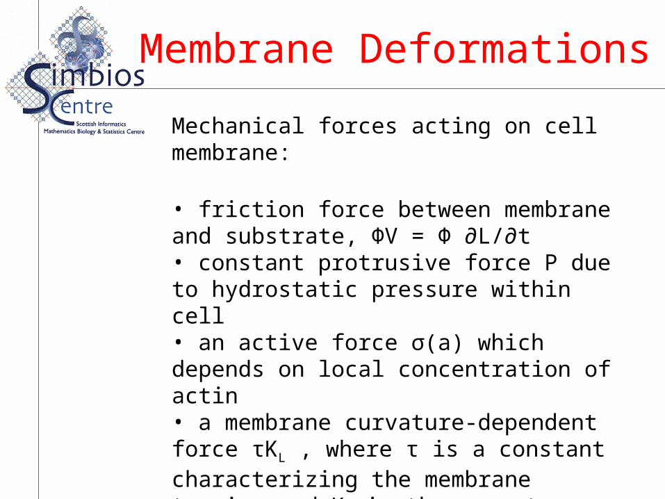
Mechanical forces acting on cell membrane:

• friction force between membrane and substrate, ΦV = Φ ∂L/∂t• constant protrusive force P due to hydrostatic pressure within cell• an active force σ(a) which depends on local concentration of actin• a membrane curvature-dependent force τΚL , where τ is a constant characterizing the membrane tension and ΚL is the curvature

Membrane Equation

LKLaPt

L

)(

where L = L(θ) denotes the radial extension of the cell cortex

.)(

),(

,0)(

2

L

ca

pcev

KLaPt

L

aakt

aaDt

a

u

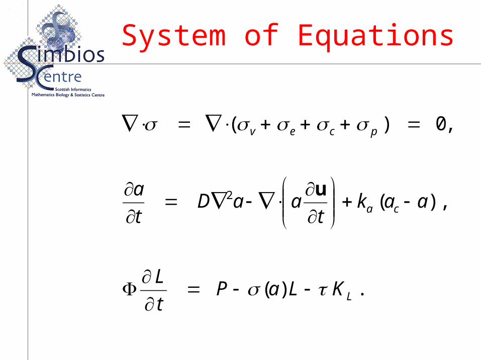
System of Equations

.

))((

))(()(2

,2

))(),((,

2/3

20

2

202

2

0

2

2/322'

2''2'

2/32'2'

''''''

RLL

RLL

RLL

K

rr

rrrrK

sysxyx

yxyxK

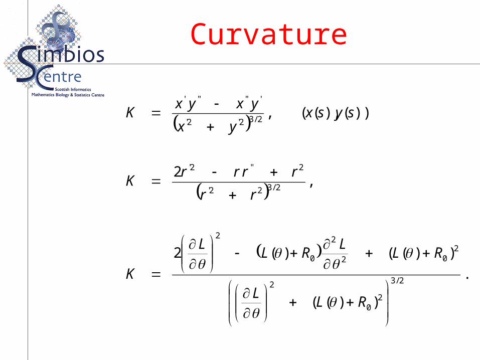
Curvature

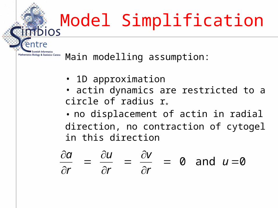
Main modelling assumption:

• 1D approximation • actin dynamics are restricted to a circle of radius r*

• no displacement of actin in radial direction, no contraction of cytogel in this direction

00

ur

v

r

u

r

a and

Model Simplification

.

2

20

11

2

1

1

2

1

0))()(][( ''21

r

vr

v

r

uv

rr

v

r

vu

r

r

v

r

vu

rr

u

paE IIII

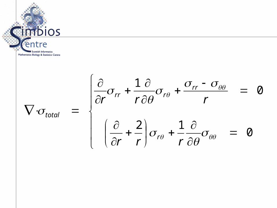
012

01

rrr

rrr

r

rrrrr

total

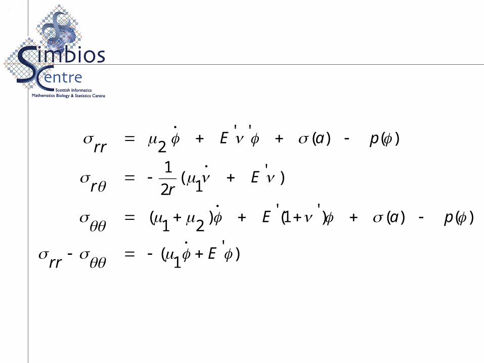
)'1

(

)()()'1(')21

(

)'1

(2

1

)()(''2

Err

paE

Err

paErr

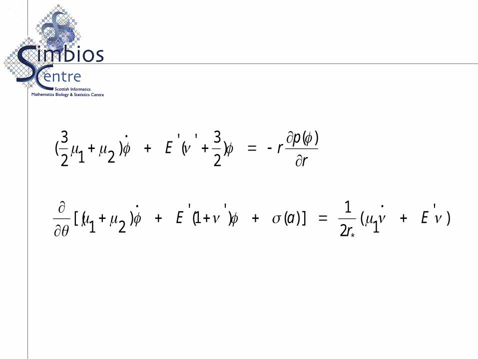
)'1

(2

1])()'1(')

21[(

)()

2

3'(')212

3(

*

Er

aE

r

prE

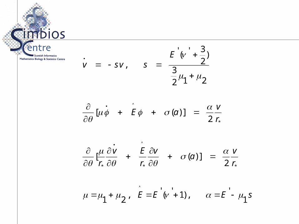
sEEE

r

va

v

r

Ev

r

r

vaE

Esvsv

1',)1'(',

21

2])([

2])([

2123

)23'('

,

***

*

Membrane and actin dynamics are coupled by means of the following equation describing the conservation of actin:

).()(1

),(),(),(

*2

2

2*

QQkvQr

Q

r

D

t

Q

tatLtQ

ca

sataa

L

eaa

KLaPt

L

aLvLar

La

r

D

t

La

r

va

v

r

Ev

r

/2

*2

2

2*

***

)(

)(

)1()(1)()(

2])(

1[0

Simplified Equations

Linear Stability Analysis

Linear stability analysis is carried out in order todetermine the conditions required for the model parameters to generate self-sustained oscillationsof the membrane – destabilization of uniform steady-state through a Hopf bifurcation

Steady State

2)()1('0

)1(

0)1(')1(

.)exp(~

0,)1(

,1

2*

*

022

*0

22

*

0

0

000

kEikr

r

Likk

r

DLk

r

DL

etciktaaa

vP

La

Dispersion Equation

The dispersion equation found from the solution of det(A) = 0, is given by:

0)()()( 22232 ckbkak

0)()()(0)(,0)( 22222 kckbkaandkaka

Figure 4. Conditions required to satisfy the Routh–Hurwitz criteria.

Static Membrane Deformations

])sin([)(

)(

0

m

KLPt

LL

Replace retraction force σ(a) by γ(θ):

α and m control amplitude of deformation and modeof deformation respectively

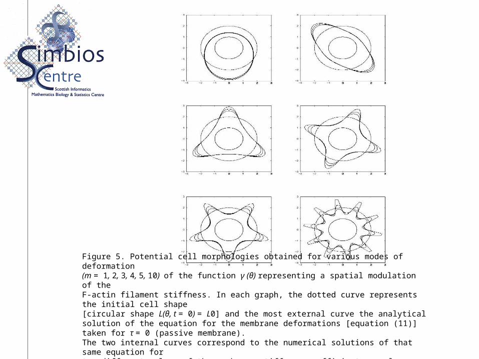
Figure 5. Potential cell morphologies obtained for various modes of deformation (m = 1, 2, 3, 4, 5, 10) of the function γ (θ) representing a spatial modulation of the F-actin filament stiffness. In each graph, the dotted curve represents the initial cell shape [circular shape L(θ, t = 0) = L0] and the most external curve the analytical solution of the equation for the membrane deformations [equation (11)] taken for τ = 0 (passive membrane).The two internal curves correspond to the numerical solutions of that same equation fortwo different values of the membrane stiffness coefficient, namely τ = 0.05 and τ = 0.1.

Dynamic Membrane Deformations

sataa

L

eaa

KLaPt

L

aLvLar

La

r

D

t

La

r

va

v

r

Ev

r

/2

*2

2

2*

***

)(

)(

)1()(1)()(

2])(

1[0

Numerical computation of equations: Crank-Nicholsonfinite differences, relaxation scheme; periodic boundary conditions; initial conditions random perturbations of F-actin concentration around homogeneous steady-state in circular morphology.

Figure 6. Simulation results of the spatio-temporal evolution of the cell membrane deformations (left side), together with the corresponding actin distributions (right side).rotating wave of deformation;

Numerical Simulation Results

L(θ,t) a(θ,t)

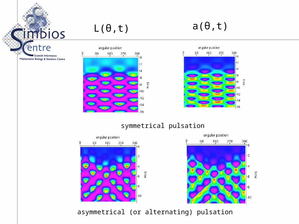
symmetrical pulsation

asymmetrical (or alternating) pulsation

L(θ,t) a(θ,t)

Figure 7. Simulated cell membrane deformations (asymptotic state associated with the topgraph of Fig. 6). Snapshots are taken every 200 iterations (_t = 0.2). The counterclockwisewave of deformation has a periodicity of about 2.8 normalized time units (sequenceto be read from top to bottom).

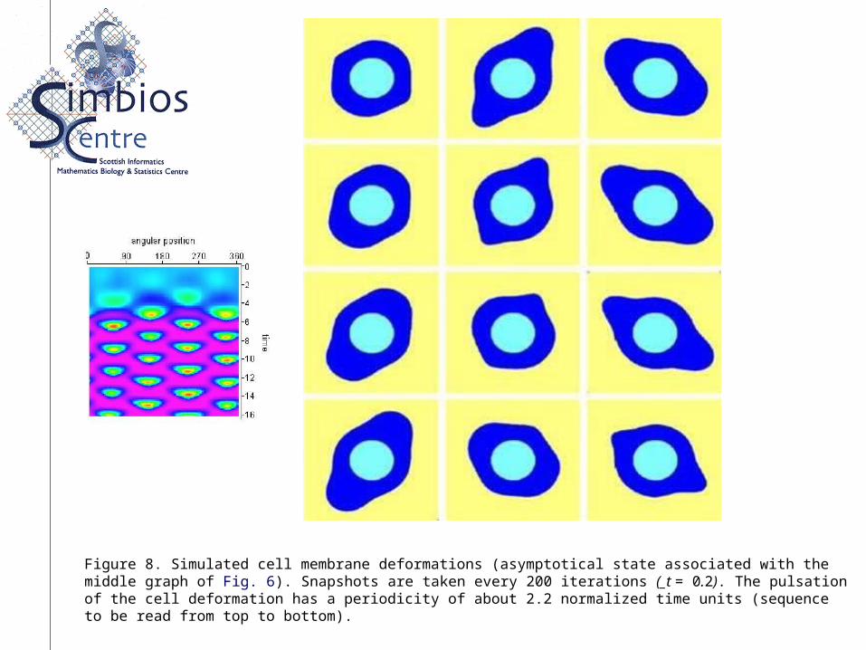
Figure 8. Simulated cell membrane deformations (asymptotical state associated with themiddle graph of Fig. 6). Snapshots are taken every 200 iterations (_t = 0.2). The pulsationof the cell deformation has a periodicity of about 2.2 normalized time units (sequenceto be read from top to bottom).

Figure 9. Simulated cell membrane deformations (asymptotic state associated with thebottom graph of Fig. 6). Snapshots are taken every 200 iterations (_t = 0.2). Thealternating pulsation of the cell deformation has a periodicity of about 2.8 normalized timeunits (sequence to be read from top to bottom).

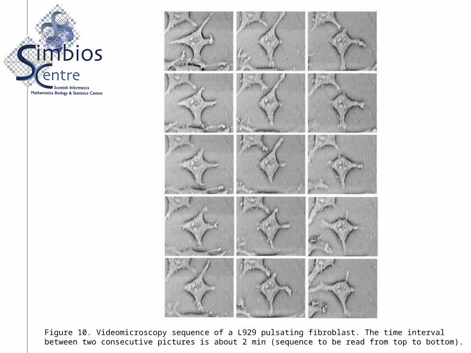
Figure 10. Videomicroscopy sequence of a L929 pulsating fibroblast. The time intervalbetween two consecutive pictures is about 2 min (sequence to be read from top to bottom).

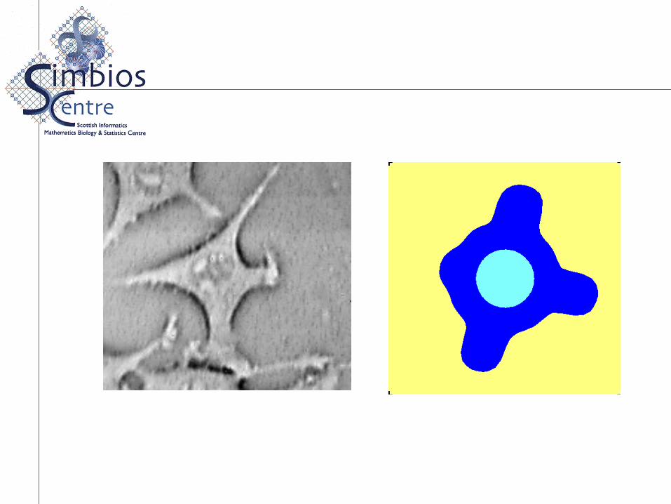
Figure 11. Simultaneous plots of actin distribution and corresponding membrane deformationsin upper graphs. In the lower rectangular graphs, the associated tangential displacementsof actin are displayed. These four graphs correspond to the snapshots 1, 3, 4and 5 of the sequence of Fig. 7 associated with the normalized times 5, 5.4, 5.6 and 5.8respectively.

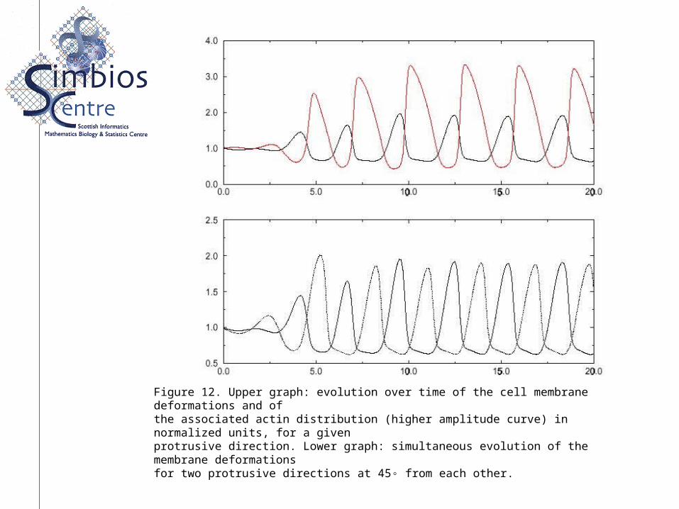
Figure 12. Upper graph: evolution over time of the cell membrane deformations and ofthe associated actin distribution (higher amplitude curve) in normalized units, for a givenprotrusive direction. Lower graph: simultaneous evolution of the membrane deformationsfor two protrusive directions at 45◦ from each other.

Figure 13. Schematic representation of a migrating cell exhibiting a characteristic domelikeshape where the thickest part represents the cell body. From the mechanical pointof view, intercalation of molecules in the membrane is responsible for cell morphologicalinstabilities.

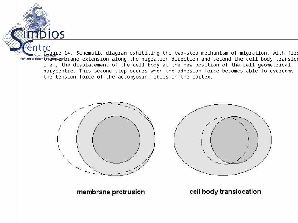
Figure 14. Schematic diagram exhibiting the two-step mechanism of migration, with firstthe membrane extension along the migration direction and second the cell body translocation,i.e., the displacement of the cell body at the new position of the cell geometricalbarycentre. This second step occurs when the adhesion force becomes able to overcomethe tension force of the actomyosin fibres in the cortex.

)()( CC

modification of membrane tension coefficient τ in presence of a chemoattractant, concentration C

where Λ(C) is a function which characterizes the sensitivity of the cell to the extracellular factor

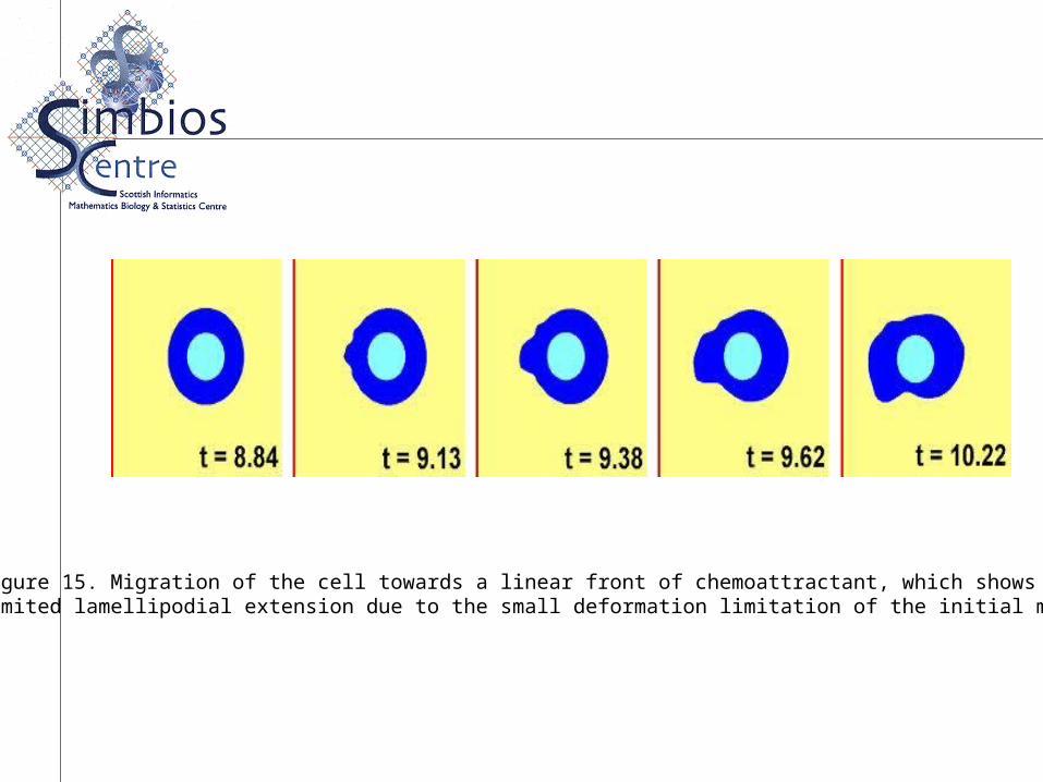
Figure 15. Migration of the cell towards a linear front of chemoattractant, which showslimited lamellipodial extension due to the small deformation limitation of the initial model.