Market Analysis & Position Sizing(Both Equally Necessary)

=

We have a plethora of market analysis, selection and timing techniques…..but

We have no method, no framework, no paradigm, for the equally important, darknether-world of position sizing.

Part 1

Optimal f

f = | Biggest Losing Outcome for 1 Unit | / f$

f$ = Account Equity / Units

Example: -$10,000 Biggest Losing Outcome, $50,000 Account, and I have on 200 shares, (2 units ):

f$ = 50,000 / 2 = 25,000

f = | -10,000 | / 25,000 = .4

Where:

Everyone, on Every Trade, on Every “Opportunity” Involving Risk,

has an f value (whether they acknowledge it or not):

(also f$ = | Biggest Losing Outcome for 1 Unit | / f

f$ and GHPR Invariant to Biggest Loss

BiggestLoss f f$ GHPR

–0.6 .15 4 1.125

–1 .25 4 1.125

–2 .5 4 1.125

–5 1.25 4 1.125

–29 7.25 4 1.125

Trajectory Cone (Bell-Shaped on all 3 Axes)

The distribution can be made into bins. A scenario is a bin. It has a probability and An outcome (P/L)

2:1 Coin Toss

0

0.1

0.2

0.3

0.4

0.5

0.6

-1 +2

Outcome

Pro

bab

ilit

y

Mathematical Expectation

2:1 coin toss: ME = .5 * -1 + .5 * 2 = -.5+1 = .5

f value example – 2:1 Coin Toss

• $10 stake• Worst Case Outcome -1• I’m wagering $5 (5 units)• f$ = 10 / 5 = 2 (one bet for every $2 in my

stake)• f =|-1| / 2 = .5• When biggest loss is manifest, we lose f%

of our stake – 50% in this case

The Mistaken Impression2:1 Coin Toss - 1 Play Expectation

0

0.25

0.5

0.75

1

1.25

1.5

1 50 99

Fraction of Stake (f)

Mu

ltip

le m

ade

on

Sta

ke

Multiple made on stake = 1 + ME/|BL| * f

(a.k.a Holding Period Return, “HPR”)

Optimal f is an Asymptote

The Real Line ( f )

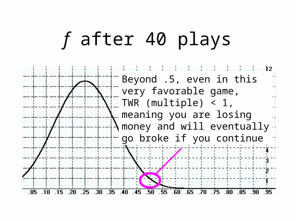
f after 40 plays

f after 40 plays

40 Plays

1 Play

f after 40 plays

At .15 and .40, makes the same, but drawdown changesAt f=.1 and .4, makes the same,

But drawdown changes!

f after 40 plays

Beyond .5, even in thisvery favorable game, TWR (multiple) < 1,meaning you are losing money and will eventuallygo broke if you continue

f after 40 plays

Points of Inflection:Concave up to concave down. Up has gain growing faster than drawdown.(but these too migrate to the optimal point as the number of holding periods grows!)

f after 40 plays

Most Favorable Blackjack Condition

Optimal f = .06 or risk $1 for every $16.67 in stake

Part 2

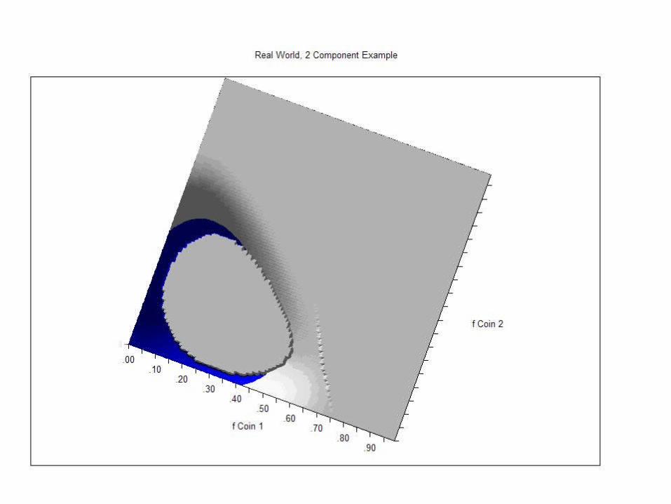
The Leverage Space Portfolio Model

Modern Portfolio Theory

Why The Leverage Space Model is Superior to Traditional (Modern Portfolio Theory) Models:

1. Risk is defined as drawdown, not variance in returns.

2. The fallacy and danger of correlation is eliminated.

3. Valid for any distributional form – fat tails are addressed.

4. The Leverage Space model is about leverage, which is not addressed in the traditional models.

Leverage has 2 Axes – 2 FacetsThe instant case of how much I amlevered up

How I progress myquantity with respectto time / equity changes

f

The fallacy and danger of correlation

• Fails when you are counting on it the most – at the (fat) tails of the distribution.

• Traditional models depend on correlation – Leverage Space model does not.

- cl/gc (all days) r=.18 (cl>3sd) r=.61 (cl<1sd) r=.09

- f/pfe (all days) r=.15 (sp>3sd) r=.75 (sp<1sd) r=.025

- c/msft (all days)r=.02 (gc>3sd) r=.24 (gc<1sd) r=.01

f after 40 plays

Why The Leverage Space Model is Superior to Traditional (Modern Portfolio Theory) Models:

1. Risk is defined as drawdown, not variance in returns.

2. The fallacy and danger of correlation is eliminated.

3. Valid for any distributional form – fat tails are addressed.

4. The Leverage Space model is about leverage, which is not addressed in the traditional models. (on both axes of “Leverage”)

Part 3

The Leverage Space Model

Software Implementation

http://parametricplanet.com/rvince/ScenariosExample.xls

Link for how to gather your data and create scenarios & probabilities:

http://parametricplanet.com/rvince/register.html

MktSysA MktSysB MktSysCJan-07 $617.00 $2,812.00 $6,189.00Feb-07 $664.00 $3,260.00 $6,570.00Mar-07 $673.00 $3,560.00 $7,369.00Apr-08 $751.00 $3,360.00 $7,916.00

May-08 $887.00 $3,681.00 $8,199.00Jun-08 $849.00 $2,946.00 $8,256.00Jul-08 $781.00 $2,873.00 $8,573.00

Aug-08 $851.00 $2,899.00 $8,713.00Sep-08 $942.00 $2,947.00 $8,388.00Oct-08 $834.00 $3,069.00 $8,817.00Nov-08 $804.00 $2,994.00 $8,938.00Dec-08 $789.00 $2,787.00 $8,545.00Jan-08 $791.00 $2,817.00 $9,168.00Feb-08 $813.00 $3,086.00 $9,410.00

Here is the data I am using (this is from the link example from the previous slide) :

Date,Equity

Jan-07,617.00

Feb-07,664.00

Mar-07,673.00

Apr-07,751.00

May-07,887.00

Jun-07,849.00

Jul-07,781.00

Aug-07,851.00

Sep-07,942.00

Oct-07,834.00

Nov-07,804.00

Dec-07,789.00

Jan-08,791.00

Feb-08,813.00

Get java at:

http://java.com/en/download/index.jsp

Part 4

The Leverage Space Model

Using The Paradigm

• We have seen how position sizing is equally as important as market analysis, selection and timing.

• The Leverage Space Model is both a (Superior) Portfolio Model, but also a Paradigm for examining “Position Sizing.”

• With this paradigm, we need no longer operate in this dark nether-world, riddled with heuristics, misinformation, and essentially mere alchemy (e.g. 1% rules, “Half Kelly,” “Fixed Ratio,” “Modern Portfolio Theory”).

Market Analysis & Position Sizing(Both Equally Necessary)

=

We have a plethora of market analysis, selection and timing techniques…..but

We have no method, no framework, no paradigm, for the equally important, darknether-world of position sizing.

http://parametricplanet.com/rvince/register.html