Market Demand, Elasticity, and Firm Revenue. From Individual to Market Demand Functions Think of an economy containing n consumers, denoted by i = 1,

Market Demand, Elasticity, and Firm Revenue

From Individual to Market Demand Functions

Think of an economy containing n consumers, denoted by i = 1, … ,n.

Consumer i’s demand function for commodity j is

x p p mji i* ( , , )1 2


The market demand function for commodity j is

If all consumers are identical then

where M = nm.

X p p m m x p p mjn

ji i

i

n( , , , , ) ( , , ).*1 2

11 2

1

X p p M n x p p mj j( , , ) ( , , )*1 2 1 2


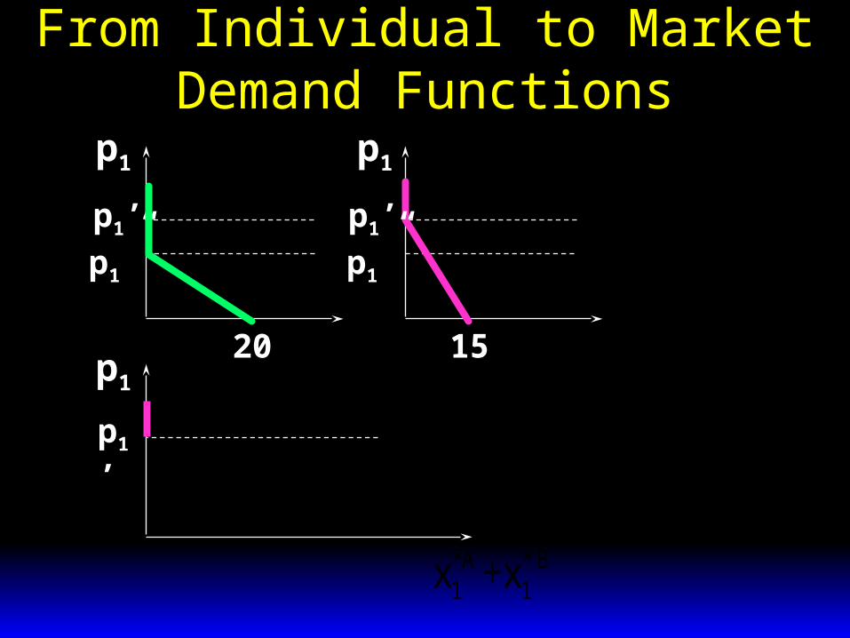
The market demand curve is the “horizontal sum” of the individual consumers’ demand curves.

E.g. suppose there are only two consumers; i = A,B.


p1 p1

x A1* x B

1*20 15

p1’

p1”

p1’

p1”


p1 p1

x A1* x B

1*

*A * B1 1x +x

p1

20 15

p1’

p1”

p1’

p1”

p1’


p1 p1

x A1* x B

1*

p1

20 15

p1’

p1”

p1’

p1”

p1’

p1”

*A * B1 1x +x


p1 p1

x A1* x B

1*

p1

20 15

35

p1’

p1”

p1’

p1”

p1’

p1”

The “horizontal sum”of the demand curvesof individuals A and B.

*A * B1 1x +x

Elasticities

Elasticity measures the “sensitivity” of one variable with respect to another.

The elasticity of variable x with respect to variable y is

,

%

%x y

x

y

Economic Applications of Elasticity

Economists use elasticities to measure the sensitivity ofquantity demanded of commodity

i with respect to the price of commodity i (own-price elasticity of demand)

demand for commodity i with respect to the price of commodity j (cross-price elasticity of demand).


demand for commodity i with respect to income (income elasticity of demand)

quantity supplied of commodity i with respect to the price of commodity i (own-price elasticity of supply)


quantity supplied of commodity i with respect to the wage rate (elasticity of supply with respect to the price of labor)

and many, many others.

Own-Price Elasticity of Demand

Q: Why not use a demand curve’s slope to measure the sensitivity of quantity demanded to a change in a commodity’s own price?


X1*5 50

10 10slope= - 2

slope= - 0.2

p1 p1

In which case is the quantity demandedX1* more sensitive to changes to p1?

X1*


5 50

10 10slope= - 2

slope= - 0.2

p1 p1

X1* X1

*



5 50

10 10slope= - 2

slope= - 0.2

p1 p1

10-packs Single Units

X1* X1

*



5 50

10 10slope= - 2

slope= - 0.2

p1 p1

10-packs Single Units

X1* X1

*

In which case is the quantity demandedX1* more sensitive to changes to p1?It is the same in both cases.


Q: Why not just use the slope of a demand curve to measure the sensitivity of quantity demanded to a change in a commodity’s own price?

A: Because the value of sensitivity then depends upon the (arbitrary) units of measurement used for quantity demanded.


1

*1

, %

%1

*1 p

xpx

is a ratio of percentages and so involves no units of measurement. Hence own-price elasticity of demand is a sensitivity measure that is independent of units of measurement.


1

*1

, %

%1

*1 p

xpx

Since demand curves are generally downward sloping, the price elasticity will most of the times be negative. So we often take the absolute value.


Elasticity depends on the necessity of the good, availability of substitutes (and switching costs to them), complements, its share in the consumer’s expenditure, time availability, short versus long-run, …

Examples of Own-Price ElasticitiesAlimentação 0.63Vestuário 0.51Sapatos 0.70Transporte 0.60Habitação 0.56Cuidados médicos 0.80Artigos de toilette 2.42Artigos desportivos 2.40Taxi 1.24Flores, sementes e plantas 2.70Teatro, Ópera 0.18Electricidade 1.20

Fontes: Economics, Dornbush e Fisher, McGraw-Hill, e Microeconomics and Behavior, Frank, McGraw-Hill.

Arc and Point Elasticities

An “average” own-price elasticity of demand for commodity i over an interval of values for pi is an arc-elasticity, usually computed by a mid-point formula.

Elasticity computed for a single value of pi is a point elasticity.

Point Own-Price Elasticity

Own-price elasticity is not constant along a linear demand curve.

It declines in absolute value as price decreases and quantity demanded increases.


pi

Xi*

a

pi = a - bXi*

a/b

i

ipX pa

pii

,*

1

0

a/2

a/2b

own-price elastic (>1)

own-price inelastic (<1)(own-price unit elastic)


i

i

i

ipX dp

dX

X

pii

*

*,*

1*

ai

i

i pakdp

dX

ap

papka

kp

pai

aia

iai

ipX ii

1

,*

X kpi ia* .E.g. Then (a<0)

so


pi

Xi*

X kp kpk

pi i

ai

i

* 22

2 everywhere alongthe demand curve

Revenue and Own-Price Elasticity of Demand

If raising a commodity’s price causes little decrease in quantity demanded, then sellers’ revenues rise.

Hence own-price inelastic demand causes sellers’ revenues to rise as price rises.


If raising a commodity’s price causes a large decrease in quantity demanded, then sellers’ revenues fall.

Hence own-price elastic demand causes sellers’ revenues to fall as price rises.


R p p X p( ) ( ).* Sellers’ revenue is



So dRdp

X p pdXdp

**

( )



So

dpdX

)p(X

p1)p(X

*

**

dRdp

X p pdXdp

**

( )



So

1)(* pX

dpdX

)p(X

p1)p(X

*

**

dRdp

X p pdXdp

**

( )


1)(* pXdp

dR


1)(* pXdp

dR

so if 1 thendRdp

0

and a change to price does not altersellers’ revenue.


1)(* pXdp

dR

but if 10 thendRdp

0

and a price increase raises sellers’revenue.


And if 1 thendRdp

0

and a price increase reduces sellers’revenue.

1)(* pXdp

dR


In summary:

Own-price inelastic demand:price rise causes rise in sellers’ revenue.

Own-price unit elastic demand:price rise causes no change in sellers’revenue.Own-price elastic demand:price rise causes fall in sellers’ revenue.

Marginal Revenue and Own-Price Elasticity of Demand

A seller’s marginal revenue is the rate at which revenue changes with the number of units sold by the seller.

( )( )

dR qMR q

dq


p(q) denotes the seller’s inverse demand function; i.e. the price at which the seller can sell q units. Then

MR qdR q

dqdp q

dqq p q( )

( ) ( )( )

R q p q q( ) ( ) so

q dp(q)=p(q) 1+

p(q) dq


q dp(q)MR(q)=p(q) 1+

p(q) dq

q

p

dp

dqand

so

1

1)()( qpqMR


1

1)()( qpqMR says that the rate

at which a seller’s revenue changeswith the number of units it sellsdepends on the sensitivity of quantitydemanded to price; i.e., upon theown-price elasticity of demand.

Selling onemore unit raises the seller’s revenue.

Selling onemore unit reduces the seller’s revenue.

Selling onemore unit does not change the seller’srevenue.


If 1 then MR q( ) .0

If 10 then MR q( ) . 0

If 1 then MR q( ) . 0


An example with linear inverse demand:

p(q)=a-bq

Then R q p q q a bq q( ) ( ) ( )

and MR(q)=a-2bq


p q a bq( )

MR q a bq( ) 2

a

a/b

p

qa/2b


p q a bq( ) MR q a bq( ) 2

a

a/b

p

qa/2b

q

$

a/ba/2b

R(q)

Income Elasticity

Inferior good: income elasticity<0Necessity: 0<income elasticity<1Luxury: income elasticity>1

Examples of Income Elasticity

Automobiles 2.46Furniture 1.48Restaurant meals 1.40Tobacco 0.64Gasoline 0.48Margarine - 0.20Pork products - 0.20Public transportation - 0.36

Source: Microeconomics and Behavior, Frank, McGraw-Hill.

Cross-Price Elasticities

Substitutes: cross-price elasticity > 0

Complements: cross-price elasticity < 0

Independents: cross-price elasticity = 0

Examples of Cross-Price Elasticities

For Butter with respect to the price of Margarine 0.81

For Beef with respect to Pork 0.28

For Entertainment with respect to Food - 0.72

Source: Microeconomics and Behavior, Frank, McGraw-Hill.

Documents

Market Demand, Elasticity, and Firm Revenue. From Individual to Market Demand Functions Think of an economy containing n consumers, denoted by i = 1,