Embed Size (px)
Citation preview

Published by
Indo – German Energy Programme
Green Energy Corridors
Market Design for an Electricity
System with higher share of RE
Energy Sources

Consortium Partners
Ernst & Young LLP, India
Fraunhofer IWES, Germany
University of Oldenburg, Germany
FICHTNER GmbH & Co. KG, Germany

Contents
1 Problem Statement 1
1.1 High Delivered Cost of RE Power 1
1.2 Burden on DISCOMs on Purchase of RE power 1
1.3 Deviation from RE Schedule 2
1.4 Non Uniform Distribution of RE potential 3
2 Current Indian power market 4
2.1 Introduction 4
2.2 Structure of Indian Electricity Market 5
2.3 Transactions in the Market 6
3 German Electricity Market 14
3.1 Regulatory Framework 14
3.2 Introductive example 15
3.3 Balancing groups 17
3.4 Market based balancing 18
3.4.1 Scheduling 19
3.4.2 Spot market 20
3.5 Product specifications 21
3.5.1 Day-ahead auctions 21
3.5.2 Orders 21
3.5.3 Price determination 24
3.5.4 Post trading period 24
3.5.5 15-min. intraday auction 25
3.5.6 Intraday continuous trading 25
3.6 Control energy or reserves for imbalances 27
3.6.1 Pricing, remuneration and settlement 27
3.7 Cross-border trading 28
3.8 Market coupling 30
3.8.1 Cross border capacity allocation 31
3.9 Network tariffs 32
3.10 Renewable Energies within the set-up of regulation and mechanisms 33
3.10.1 Funding and refinancing 33
3.10.2 Marketing of RE and conformity with balancing group concept 34
3.10.3 Impact on short-term markets and consequences 35
4 Ancillary Services (AS) 40
4.1 Development of joint operational procedures 41
4.2 Organizational Implementation of the Frequency Control 42
4.2.1 Control activities 42
4.2.2 Assessment of balancing needs and level of responsibility 45
4.3 Methodology of reserve dimensioning 53
4.3.1 Primary reserve 54
4.3.2 Secondary and minute reserve 55
4.4 Specification of reserves 58
4.4.1 Prequalification 58
4.4.2 Product specifications 59
4.4.3 Recommendation for the introduction of restoration reserve as ancillary
service 61
4.4.4 Implementation of grid control cooperation 62
4.5 Voltage control 64
4.5.1 Market design for voltage support 65
4.5.2 Examples of current approaches to contract voltage support in Europe 65
4.5.3 Voltage support by RES 66
4.6 Black start 67
4.7 RES capabilities to provide ancillary services 67
4.8 German Scenario 71
4.8.1 Primary control reserve 71
4.8.2 Secondary control reserve 71
4.8.3 Tertiary control reserve 71
4.8.4 Grid control cooperation 72
4.9 Status of ancillary services in India 73
4.9.1 Definition and Scope 73
4.9.2 CERC Draft Regulation on Ancillary Services Operation, May 2015 74
4.9.3 Petition on the inadequate response of FGMO, February 2015 74

5 Market Options 75
5.1 Market Models 75
5.2 Pricing Models 77
6 Balancing Group Concept 79
6.1 Formation of balancing groups 79
6.2 Balance Responsible Party 80
6.3 Cost of Ancillary Services and Reserves 80
6.4 Timeline of rollout 80
6.5 Participants and Roles 80
6.5.1 System Operators 80
6.5.2 BRPs 82
6.6 Demand Response in Balancing Groups 83
7 Transition to Proposed Market Design 85
7.1 Phase 1 86
7.1.1 Modifications to regulations related to Power Purchase Agreements 86
7.1.2 New Products in the market 87
7.1.3 Introduction of Generator only Balancing Groups & Reserve Products 87
7.1.4 Introduction of Generator Only Balancing Groups 88
7.1.5 Congestion Management 89
7.1.6 Flexible Generation 89
90
7.2 Phase 2 90
7.3 Required Legislative and Regulatory Changes 90
7.3.1 Introduction of Consumers in Balancing Groups 91
7.3.2 Introduction of Demand Side Products 91
7.3.3 Load Forecasting 91
7.3.4 Review of Balancing Group Regional Restrictions 91
7.3.5 Migration of PPAs 91
7.4 Phase 3 93
7.4.1 Modification of Products on PXs 93
7.4.2 Migration of PPAs 93
7.4.3 Review of RPO/REC 93

7.5 Proposed Market Design for India 95
7.5.1 Market Design 95
7.6 Deviation and mechanism of settlement 98
Management of Schedule Deviations due to RE 98
Remuneration to RE Generators and Aggregators 98
7.7 Control Reserves (Ancillary Services and Balancing) 99
7.7.1 Contracting of reserves 99
7.7.2 Scheduling of reserves 99
7.7.3 Activation of Reserves 100
7.7.4 Infrastructure for Deployment of Reserves 100
7.7.5 Payment to reserve service providers 101
7.7.6 Reserve service providers 101
7.7.7 Penalty for defaulting reserve providers 102
8 Roadmap and Summary of Recommendations 103
8.1 Immediate Steps – Over the next 5 years (Phase 1 of transition) 103
8.2 Steps to be taken after 5 years up to 10 years (Phase 2 of transition) 103
8.3 Steps to be taken after 10 years up to 15 years (Phase 3 of transition) 104
9 Bibliography 105
Annexure 1 110
Annexure 2 1
Annexure 3 7
Annexure 4 11
a. Single Part Tariff 11
b. Two Part Tariff 12
c. Availability Based Tariff 13
List of Figures
Figure 1: Wind and Solar Generation Gujarat 2014 and 2022 (projected) ............................................. 2
Figure 2: Variation of Wind and Solar potential in India .......................................................................... 3
Figure 3: Segments of Indian Power Sector ........................................................................................... 4
Figure 4: Structure of Indian Power Market ............................................................................................ 5
Figure 5: Classification of Indian Power Market...................................................................................... 7
Figure 6: Transactions in Indian Power Market ...................................................................................... 8
Figure 7: Regulatory Transition of Indian Power Market ........................................................................ 9
Figure 8: Percentage Distribution of Contracts in the Market ................................................................. 9
Figure 9: Functioning of Day Ahead Markets ........................................................................................ 10
Figure 10: Timeline of trades on the IEX under 24 hour operations ..................................................... 11
Figure 11: German electricity markets. (Fraunhofer IWES based on (Judith et al. 2011)) ................... 14
Figure 12 Interaction of two BRPs and a TSO in a control zone regarding scheduling and imbalance
settlement .............................................................................................................................................. 16
Figure 13: Estimated marginal cost based merit-order for all German power plants ........................... 19
Figure 14: Share of trading volume of national EPEX SPOT market in annual national (EPEX SPOT
2014f) .................................................................................................................................................... 20
Figure 15: Example of an individual offer curve at EPEX SPOT representing the up to 256 possible
price-quantity combinations .................................................................................................................. 21
Figure 16: Possible block orders of the day-ahead auction at EPEX SPOT (EPEX SPOT 2014b) ..... 22
Figure 17: Principles of price convergence in coupled electricity markets (PCR 2014b) ..................... 30
Figure 18: Concept of direct marketing & refinancing RE ..................................................................... 33
Figure 19: Portfolio size of 30 selected direct marketing companies ................................................... 35
Figure 20: Electricity production by source and price development at EPEX spot markets ................. 37
Figure 21: Illustrative example: Marginal cost pricing mechanism and merit-order effect of RE .......... 38
Figure 22: Spot market price and total RE, wind and PV share of gross electricity consumption in
Germany................................................................................................................................................ 39
Figure 23: Survey of important system characteristics and services .................................................... 40
Figure 24: Dynamic hierarchy of Load-Frequency Control processes in Europe, Source: entso-e ..... 43
Figure 25: Types and hierarchy of geographical areas in Load-Frequency Control processes in
Europe and a possible configuration of a synchronous area, Source: entso-e .................................... 44
Figure 26: Current status of Synchronous Areas, LFC Blocks and LFC Areas in Europe, Source:
entso-e .................................................................................................................................................. 44
Figure 27: Load Frequency Control Block Diagram with Input ∆PL and Output ∆f .............................. 46
Figure 28: Steady state frequency deviation for different shares of RE - no speed regulation ............ 47

Figure 29: Steady state frequency deviation for different shares of RE – 50% conventional generation
with speed regulation R =5% ................................................................................................................ 48
Figure 30: Steady state frequency deviation for different shares of RE – 100% conventional
generation with speed regulation R=5% ............................................................................................... 49
Figure 31: Steady state frequency deviation for different shares of RE – 50% conventional and 100%
RE generation with speed regulation R=5% ......................................................................................... 49
Figure 32: Steady state frequency deviation for different shares of RE - all generation with speed
regulation R=5% .................................................................................................................................... 50
Figure 33: Influence of primary control on frequency deviation in terms of RES schedule deviation of
30% ....................................................................................................................................................... 51
Figure 34: Allowed deviation from schedule of RE indicating limits of 30% and 12% .......................... 51
Figure 35: Allowed deviation from schedule of RE indicating limits of 30% and 12% with variable
primary control provision. ...................................................................................................................... 52
Figure 36: Simplified illustration of imbalance types (source: entso-e) ................................................ 53
Figure 37: Schematic representation of the Graf-Haubrich method ..................................................... 56
Figure 38: Procured secondary reserve capacity in Germany for each quarter of the year ................. 57
Figure 39: Procured minute reserve capacity in Germany for each quarter of the year ....................... 57
Figure 40: Model protocol for the prequalification of a technical unit for positive primary control ........ 59
Figure 41: Technical implementation of Imbalance Netting in IGCC .................................................... 63
Figure 42: Example of pro-rata distribution of netting potential with congestion correction ................. 63
Figure 43: Value of netted imbalances per country .............................................................................. 64
Figure 44 - Market Options ................................................................................................................... 75
Figure 45 - Types of electricity pool options ......................................................................................... 76
Figure 51: Organization of Intra state balancing groups ....................................................................... 81
Figure 52: Organization of Inter-state Balancing Groups ..................................................................... 82
Figure 53 - Demand Response ............................................................................................................. 84
Figure 46: Current Power Market .......................................................................................................... 86
Figure 47: Market on complete implementation of phase 1 .................................................................. 90
Figure 48: Market structure after complete implementation of Phase 2 ............................................... 92
Figure 49: Market on Completion of Phase 3 ....................................................................................... 94
Figure 50 - Proposed Market Design .................................................................................................... 96
Figure 54: Block diagram of a generator-load model (Kundur, 1994) .................................................... 3
Figure 55: Governor Steady-State Speed Characteristics (Saadat) ....................................................... 4
Figure 56: Block Diagram of Governor with Frequency Control Loops for Steam Generator Unit
(Saadat)................................................................................................................................................... 5
Figure 57: Load Frequency Control Block Diagram with Input ∆PL and Output ∆f ................................ 6
Figure 58: Single Part Tariff Structure .................................................................................................. 12

Figure 59: Two Part Tariff Structure ...................................................................................................... 13
Figure 60: Components of ABT ............................................................................................................ 14
Figure 61: Gujarat Load Demand - 2014 and 2022 .............................................................................. 16
Figure 62: Gujarat Solar Generation for July 2014 and July 2022........................................................ 16
Figure 63: Gujarat Wind Generation for July 2014 and July 2022 ........................................................ 17
Figure 64: Gujarat RE Generation for July 2014 and July 2022 ........................................................... 17
Figure 65: Gujarat Load Demand v/s RE Generation & Residual Load for July 2022.......................... 18
Figure 66: Frequency Deviation for Different Shares of RE ................................................................. 19
Figure 67 - Forecasted GHI series ........................................................................................................ 28
Figure 68 - IFS gridded map of Rajasthan ............................................................................................ 29
Figure 69: Change in Forecast Error for a Regional and Single Site Forecast .................................... 30
Figure 70: Accuracy of forecast for different Prediction Horizons......................................................... 31
Figure 71: Scatter plot linking forecast error to actual generation in % of total installed capacity ........ 32
List of Tables
Table 1: Type of Contracts in Term-Ahead Market ............................................................................... 11
Table 2: Difference between Day Ahead Contingency and Day Ahead Spot Contracts ...................... 12
Table 3: Summary of Term-Ahead Market ............................................................................................ 13
Table 4: EPEX SPOT day-ahead auction contracts specifications (EPEX SPOT 2015) ..................... 23
Table 5: EPEX SPOT 15-min. intraday auction contracts specifications (EPEX SPOT 2015) ............. 25
Table 6: EPEX SPOT intraday continuous trading one hour contracts specifications (EPEX SPOT
2014e) ................................................................................................................................................... 29
Table 7: Classification of ancillary and operational services in Germany ............................................. 41
Table 8: SOC and Regional group activities ......................................................................................... 42
Table 9: Error types considered in the Graf-Haubrich method (CONSENTEC 2010) .......................... 56
Table 10: Parameterization of the Graf-Haubrich method (CONSENTEC 2010) ................................. 56
Table 11: Reserve product specifications ............................................................................................. 60
Table 12 - Factors influencing demand and supply of the control reserve market in Germany ........... 61
Table 13: Wind and Solar PV Technology Capabilities for Gas Provision ........................................... 68
Table 14: Explanations and References for Wind and Solar Technology Capabilities ........................ 70
Table 15: Requirements of the different types of control reserves ....................................................... 73
Table 16 - Comparison of Market Options ............................................................................................ 77
Table 17: Proposed Products on the Power Exchange ........................................................................ 87
Table 18: Requirement of Different types of control reserves ............................................................ 102
Table 22: Proposed Deviation Settlement for RE Generators .............................................................. 22
Table 23: Analysis of RRF and Proposed DSM for RE Generators ..................................................... 24
Table 24: Per Unit Charges for a Wind Generator as per Proposed DSM Mechanism ....................... 25
Table 25: Analysis of RRF and Proposed DSM for RE Generators for deviation within ±12% ............ 26
Table 26: Impact of Proposed DSM Mechanism due to different PPA Rates ...................................... 32

1 | P a g e
1 Problem Statement
Large scale integration of Renewable Energy (RE) into a power system poses multiple technical and
commercial challenges to the stake holders of the system. It is critical to address these challenges for
large scale integration of RE into the power system. This section of the report describes the major
techno-commercial challenges faced by RE grid integration.
1.1 High Delivered Cost of RE Power
The delivered cost of power refers to the actual expense incurred for the total quantity of power
delivered at the metering point. The overall high delivered cost of RE power is a major deterrent in the
large scale adoption of RE.
Cost of Interstate Transfer of RE
The delivered cost of RE power increases in the case of an interstate transfer of power. This increase
is the result of addition of charges linked to wheeling, transmission and losses. RE power therefore
becomes uncompetitive in the power market, leading to the requirement of Renewable Purchase
Obligations (RPOs) to ensure it’s off take.
Cost of RE above APPC
The cost of RE power to DISCOMS is higher than APPC in all states. This makes the purchase of RE
power a loss making business decision to DISCOMS.
To bridge the gap between delivered cost of RE power and delivered cost of conventional generation,
many states have introduced exemptions by policy on cost of transmission of RE power. Since wind
energy is more mature and intensively promoted (especially over the past 2 decades), it has lower
tariffs in comparison to solar power. It is estimated that solar PV is expected to achieve parity with
conventional power in the in the coming years with falling price of PV systems and rising price of retail
electricity. Till RE power becomes competitive in the market, there is a need to incentivise the sale of
RE power to make the upcoming capacity addition economically viable.
1.2 Burden on DISCOMs on Purchase of RE power
DISCOMs’ debt burden was INR 3.04 lakh crore and accumulated loss was INR 2.52 lakh crore
adding up to a total of INR 5.56 lakh crores as of June 2015. Most DISCOMS in India are operating in
losses, primarily due to inefficient revenue recovery systems. According to the UP electricity regulator,
of 3.54 crore households in the state, only 1.14 crore have registered electricity connections. Out of
these registered connections, only 70.67 lakh are metered connections. This implies that out of every
100 users only 35 were paying1.
There is unwilling to raise power tariffs to recover the cost and therefore DISCOMs are unable to buy
the quantum of power they need. The provision of subsidised electricity to farmers and residential
consumers further increases this burden.
Sale of RE power in India is mainly driven by obligation enforced through regulation. DISCOMs are
one of the largest consumers of RE power in the country. Purchase of RE power is an additional
financial burden on the DISCOMs that are already financially stressed. Owing to the cost implications
of buying expensive RE power, DISCOMs fail to meet RPO targets. This increases investment risk of
RE power and is therefore a major deterrent to RE developers. In certain cases the DISCOMs are
liable to pay a penalty for failure to meet RPO targets. However these penalties are not strictly
1 http://www.assocham.org/newsdetail.php?id=5003

2 | P a g e
enforced across all states. There is therefore an imminent need to develop a market mechanism for
the sale of RE power that reduces the burden on DISCOMs.
1.3 Deviation from RE Schedule
The deviation from RE schedule is due to the error in forecast of RE power generation. The error in
RE power forecast occurs because actual RE power generation depends on fluctuating weather
conditions. This variable nature of RE power is represented by the following plots of actual wind and
solar generation in Gujarat over the period of a month in 2014 and 2022(projected).
Figure 1: Wind and Solar Generation Gujarat 2014 and 2022 (projected)
There is an urgent need for Ancillary Services (AS) to support the power system when large quantities
of RE is integrated into the grid. Forecasting RE generation and estimating balancing requirement
would help manage the overall variability in the system. However the error in forecasting leading to
deviation from schedule would requires AS for mitigation. The cost of provisioning AS would be a
financial burden on the central and state governments.
In the current market scenario the cost of AS cannot be loaded onto RE generators because:
a) Additional costs would reduce the economic viability and competitiveness of RE generators
and would deter investors.
b) All disturbances in the power system do not originate from RE sources. There is also a
requirement of Ancillary Services to manage the variability of the power system due to
conventional generation as well as consumers deviating from schedule.
There is therefore a need to develop a market mechanism to meet the requirement of introducing AS
in the Indian power system.
-
1,000
2,000
3,000
4,000
5,000
6,000
7,000
1
69
13
7
20
5
27
3
34
1
40
9
47
7
54
5
61
3
68
1
Totr
l RE
Ge
ne
rati
on
in M
W
Hours of Month
Wind Generation for July 2014 & 2022
Wind Generation 2014
Projected Wind Generation 2022
-
1,000
2,000
3,000
4,000
5,000
6,000
1
69
13
7
20
5
27
3
34
1
40
9
47
7
54
5
61
3
68
1
Totr
l RE
Ge
ne
rati
on
in M
W
Hours of Month
Solar Generation for July 2014 & 2022
Solar Generation 2014
Projected Solar Generation 2022

3 | P a g e
1.4 Non Uniform Distribution of RE potential
RE potential of a region is based on its geographical features which vary significantly across the
country. The state wise estimated wind and solar power potential are depicted in the figures below.
Figure 2: Variation of Wind and Solar potential in India
Source: MNRE 2014, NIWE 2014
The uneven spread of RE potential across different states would create a disparity in the
RE/Conventional generation mix in different parts of the country. This would necessitate evacuation of
RE power out of the RE rich states. Profitable interstate trade of RE power is therefore needed to
ensure offtake of upcoming RE capacity and optimal utilisation of India’s RE potential.
0 20000 40000
Uttarakhand
Kerala
Uttar Pradesh
Orissa
MadhyaPradesh
Rajasthan
Jammu &Kashmir
Maharashtra
Karnataka
Tamil Nadu
AndhraPradesh
Gujarat
Wind Potential (MW) @ 80m
Estimated Potential (MW) @ 80m0 50 100 150
Goa
Tripura
Haryana
Meghalaya
Nagaland
Mizoram
Bihar
Uttarakhand
Jharkhand
Telangana
Karnataka
Himachal…
Andhra Pradesh
Maharashtra
Rajasthan
Solar Potential (GWp)
Solar Potential (GWp)

4 | P a g e
2 Current Indian power market
2.1 Introduction
Source: CEA report, March 2015 http://www.cea.nic.in/reports/planning/dmlf/growth_2015.pdf2
The state electricity boards (SEBs) and central utilities have maximum market share in the
transmission and distribution segments of the Indian power market. In the generation space, out of
the overall capacity of 271GW, the share of central, private and state utilities stand at 72GW, 104GW
and 95GW, respectively. The recent emphasis of policy and regulatory framework, as guided by the
provisions of the Electricity Act, 2003, is on bringing in competition, private sector participation and
independent regulation.
The main enablers for competition are as follows:
Generation is de-licensed (except large hydro and nuclear projects) and now all new
generation in the private sector has to be contracted through the competitive bidding route.
Open access on common carrier principle is allowed on transmission networks and is soon to
be phased in on distribution networks as well.
Provisions for parallel distribution networks in existing areas are made. This would create a
competitive environment in distribution.
Prior to 2003 and prior EA 2003, power exchanges between states/vertically integrated utilities
were majorly of small or intermittent volumes. Transactions were predominantly in nature of
emergency support. The exchanges were majorly limited due to lack of transmission inter
connections. There had been sustained shortages both in energy and peak demand which
discourages initiatives and for long there had been scepticism about success of trading.
2 http://powermin.nic.in/JSP_SERVLETS/internal.jsp
Figure 3: Segments of Indian Power Sector
5 | P a g e
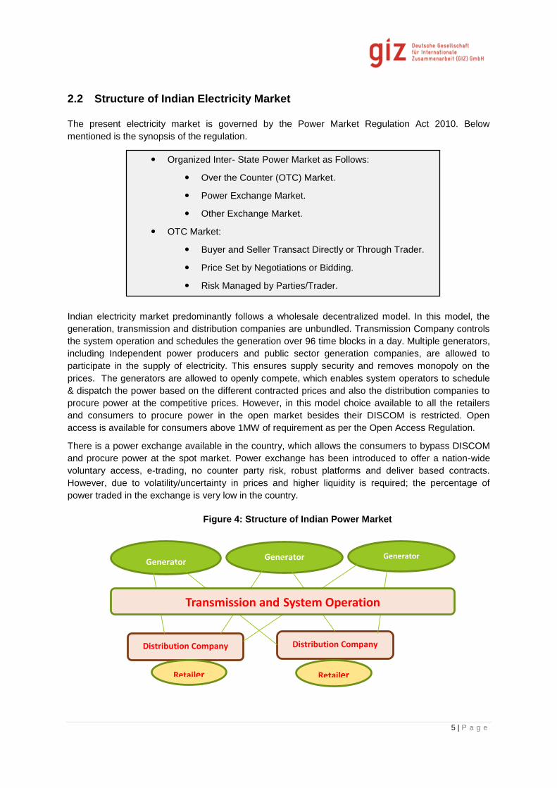
2.2 Structure of Indian Electricity Market
The present electricity market is governed by the Power Market Regulation Act 2010. Below
mentioned is the synopsis of the regulation.
Indian electricity market predominantly follows a wholesale decentralized model. In this model, the
generation, transmission and distribution companies are unbundled. Transmission Company controls
the system operation and schedules the generation over 96 time blocks in a day. Multiple generators,
including Independent power producers and public sector generation companies, are allowed to
participate in the supply of electricity. This ensures supply security and removes monopoly on the
prices. The generators are allowed to openly compete, which enables system operators to schedule
& dispatch the power based on the different contracted prices and also the distribution companies to
procure power at the competitive prices. However, in this model choice available to all the retailers
and consumers to procure power in the open market besides their DISCOM is restricted. Open
access is available for consumers above 1MW of requirement as per the Open Access Regulation.
There is a power exchange available in the country, which allows the consumers to bypass DISCOM
and procure power at the spot market. Power exchange has been introduced to offer a nation-wide
voluntary access, e-trading, no counter party risk, robust platforms and deliver based contracts.
However, due to volatility/uncertainty in prices and higher liquidity is required; the percentage of
power traded in the exchange is very low in the country.
Generator
Organized Inter- State Power Market as Follows:
Over the Counter (OTC) Market.
Power Exchange Market.
Other Exchange Market.
OTC Market:
Buyer and Seller Transact Directly or Through Trader.
Price Set by Negotiations or Bidding.
Risk Managed by Parties/Trader.
Power Exchange:
Transactions on Standard Platform.
Price Set by Market Rules.
Other Exchange Market:
Derivative Product.
Figure 4: Structure of Indian Power Market
Generator Generator Generator
Distribution Company Distribution Company
Retailer Retailer
Transmission and System Operation

6 | P a g e
The above mentioned summarizes broadly a market model followed in the country. The power can
either be directly sold by the generation companies to the distribution companies or through an
intermediary i.e. an independent body who can purchase power in bulk. However there can be
change in orientation of the above model from state to state which is discussed as under.
In Rajasthan, the DISCOMs are purchasing power directly from RVUNL, which is the generation
company responsible for the development, operation and maintenance of state owned power stations.
Rajasthan DISCOM Power Procurement Centre (RDPPC) has been established for purchase of
power on behalf of the DISCOMs. The 3 DISCOMs in Rajasthan are Jaipur Vidyut Nigam Ltd, Ajmer
Vidyut Vitran Nigam Ltd and Jodhpur Vidyut Vitran Nigam Ltd.
In Gujarat, the Gujarat State Electricity Corporation Ltd. (GSECL) is the power generation company.
The vertically integrated GEB was unbundled into seven companies one each for generation and
transmission, four distribution companies (DISCOMs) and a holding company known as Gujarat Urja
Vikas Nigam Limited (GUVNL). The generation, transmission and distribution companies have been
structured as subsidiaries of GUVNL. GUVNL acted as the planning and coordinating agency in the
sector when reforms were undertaken. It is now the single bulk buyer in the state as well as the bulk
supplier to distribution companies. It also carries out the function of power trading in the state.
Presently, there are four DISCOMs in Gujarat; UGVCL, DGVCL, MGVCL and PGVSL.
In Andhra Pradesh, the generation company is Andhra Pradesh Power Generation Corporation
(APGENCO). Post the state bifurcation and as per the AP Reorganization Act 2014, the NPDCL,
CPDCL, EPDCL, SPDCL have become TGNPDCL, TGSPDCL, APNPDCL and APSPDCL. The
DISCOMs in Andhra Pradesh are Southern Power Distribution Company (APSPDCL) and Northern
Power Distribution Company (APNPDCL). These DISCOMs directly purchase power from the
generating companies through PPAs.
In Karnataka, there exist PPA’s between the generation company i.e. Karnataka Power Corporation
Limited (KPCL) and Power Company of Karnataka Limited (PCKL) which is a body established to
purchase power on behalf of the five DISCOMS. The five DISCOMS in Karnataka are BESCOM,
HESCOM, MESCOM, GESCOM and CESC.
In Tamil Nadu, no independent body exists and power is purchased directly from the generation
companies. Tamil Nadu Generation and Distribution Corporation (TANGEDCO) is the only DISCOM
present and responsible for power generation and procurement.
In Himachal Pradesh, the Himachal Pradesh State Electricity Board, having its registered office in
Vidyut Bhawan, Shimla is responsible for supply of quality power to all categories of consumers’ at
most economic rates. It’s the only body responsible for power generation and supply.
2.3 Transactions in the Market
The overall market transaction comprises of Long term, Medium Term and Short term transactions.
The country has an overall peak demand of 140GW as on 2015. The demand of the country is
managed by the system operator by allocating the market transacted contracts such that it optimally
and efficiently manages the load curve. In order to manage the demand in the country, the market
transactions are scheduled such that
Base and Intermittent load- Managed by Long Term PPAs
Seasonal Variations – Managed through Short Term trades, by Traders, Bilateral Contracts or
Banking Arrangements
Daily Variations – Managed through Day ahead Power Exchange or DSM Balancing

7 | P a g e
Figure 5: Classification of Indian Power Market
In Indian electricity market, bulk power supply is tied up with Long Term (LT) agreements/contracts
which have long time period. The bulk power suppliers include predominantly the central generating
stations, state generating stations and few IPPs. DISCOMs who are obligated to supply electricity to
their consumers prefer and predominantly rely upon the long term contracts. Long term contracts
secure a base load electricity supply in the country. Moreover, it is not economically feasible for the
DISCOMs to purchase short contracts to meet the seasonal variations. It can be observed that in the
Indian electricity market, nearly 89% of power purchase agreements fall in the category of Long Term
contracts.

8 | P a g e
Figure 6: Transactions in Indian Power Market
Short Term (ST) contracts in the electricity market majorly refer to contracts less than one year period.
The contracts include electricity transactions through
Bilateral transactions through interstate trading licensees
Bilateral transactions directly by Distribution Licensees (DISCOMs)
Power Exchanges (IEX and PXIL)
Unscheduled interchange
Several regulatory interventions have enabled the successful creation and operation of Power
Exchange market. This market provides a platform on which power can be transacted in shorter time
duration/period. Two exchanges namely Power Exchange India Limited (PXIL), Indian Electricity
Exchange (IEX) are fully operation from 2008. This representation is primarily with respect to IEX as it
hosts 96% of the total volume traded on the exchanges. As per the CERC order dated 8.4.2015 on
extended market sessions. The power exchanges in India now operate for 24 hours; this however
does not mean that all products are traded for all 24 hours. Different products have different trade
windows as explained in this section.
These short term contracts cater to just 5% of the existing electricity market structure. However, these
contracts play a very crucial role in managing the peak demand and handling the intraday
imbalances.

9 | P a g e
Figure 7: Regulatory Transition of Indian Power Market
Several different contracts are executed in the power exchange market which includes namely
Intraday, Day Ahead Market (DAM), Day Ahead Contingency (DAC) contracts, daily contracts and
weekly.
Figure 8: Percentage Distribution of Contracts in the Market
Two power exchanges work in tandem and handle same or at times different electricity
contracts/products. Nevertheless, both the exchanges offer Day-ahead products.
Day-ahead Services

10 | P a g e
This service facilitates the electricity to be procured and to be scheduled for one day ahead (d) in
every 15 minutes time block. Physical electricity trading market which facilities contract for deliveries
for any/some/all 15 minute time blocks in 24 hours of next day starts from midnight. Prices of
electricity traded are determined using double sided auction bidding. The procedures are guided by
CERC- Open Access Inter-state transmission regulations, 2008.
Typical order types are:
Hourly orders
Block orders
Consecutive orders
Minimum size of the contract to be traded should be 0.1MW and the minimum quotation step is Rs. 1
per MWh. Power exchanges at 15:00hr on the present day (d-1) calculates the area clearing price
based on the transmission network availability and send the scheduling request to NLDC. Periphery
of the regional transmission in which grid entity is connected will be the delivery point. Settlement
mechanism occurs on a daily basis and is calculated based on the formula of Area Clearing Price
(ACP) X Traded volume.
Detailed procedures for day-ahead services have been provided in the form of functional diagram
below.
Day Ahead markets
The Day Ahead Markets open at 10:00 hrs every trading day, Trading days are as defined by the IEX
trading calendar. The DAM functions from 10:00 hrs to 12:00 hrs every day. Till 12:00 market players
are allowed to bid for the buying or selling of power. Between 12:00 to 13:00 the bids are matched
and the market clearing price (MCP) as well as the market clearing volume (MCV) re calculated. This
data is then sent to the respective dispatch centres for checking availability of corridors. The
availability of funds is also verified in this period. At the 15:00 hours the actual clearing price (ACP) as
well as the actual clearing volume (ACV) is published and this data is forwarded to the respective
SLDCs for verification. Market is split if there are transmission constraints; this creates different
clearing prices and volumes for different market regions. At 17:30 the NLDC clears the final schedule
and forwards it to the respective SLDCs for incorporation into despatch schedule. The illustration
below graphically depicts the operation of the Day-Ahead markets.
Figure 9: Functioning of Day Ahead Markets
Source: IEX
CERC in August 2009 allowed a Term Ahead/Additional Contracts to be traded through power
exchange. Both the exchanges commenced their operations since September 2009.
Term-Ahead Market (TAM)

11 | P a g e
TAM provides a range of products allowing the participants to buy/sell electricity for contracts beyond
day-ahead market besides intraday contracts. Four different services under TAM are tabulated
below:
Table 1: Type of Contracts in Term-Ahead Market
S.No. Contract Trading
1. Intra Day contract Trading on delivery day few hours before delivery.
3. Day Ahead contingency contract Trading to a day before delivery and after DAM
auction.
4. Daily contract Trading up to 1 Week in advance for any calendar
day starting from the 4th day of the month
5. Weekly contract Trading up to 11 days in advance
In Term Ahead Markets, the price of electricity between the producer and consumer is estimated
through way of a double sided auction. This begins with a Bid Entry where the buyers and sellers bid
their maximum and minimum prices respectively. Under this mechanism, buy trades are settled at or
below the quoted price and sell trades are settled at or above the quoted price. Based on this a
matching price is established, ensuring maximum benefits to both buyers and sellers of electricity.
This is then included in the day-ahead schedules. This is a bilateral contract between the buyer and
the seller and there is complete anonymity of the bids between them. Clearing is then done by the
SLDC and exchange and final settlement is done when the clearance is accepted by the RLDC.
The services under TAM can be further explained as follows, Timelines of products are illustrated
below:
Figure 10: Timeline of trades on the IEX under 24 hour operations

12 | P a g e
Source: IEX
1. Intra Day Contracts
The Indian power markets now operate for 24 hours, in the past the seller could only submit bids from
his own region, whereas a buyer can buy any regional contract. These contracts are available for
trading from 10:00 hrs To 20:00 hrs. on a daily basis through continuous trading process. By 20:30,
all funds are blocked including transmission and operating charges. After blocking the funds, pay-out
is done on the T or T+2 basis and the nodal RLDC is also paid its charges on T+2 basis (where T is
trading day).
In the current organisation of the power markets, the trading of products timelines is as below.
2. Day Ahead Contingency Contracts
In these contracts, for the first hour, selling bids are allowed region wise, followed by buy bids. Buyers
are allowed to see the price and region of the seller but the seller’s identity is not revealed and the
same auction mechanism with differential pricing issued. These contracts auction for all the 24 hours,
subdivided into hourly contracts and the pay-in and pay-out is on T+1 basis.
Though the Day Ahead Contingency Contracts Market appears similar to Day Ahead Spot Contracts
Market, there are subtle differences in the functioning of both. Some noticeable differences being:
Table 2: Difference between Day Ahead Contingency and Day Ahead Spot Contracts
Day Ahead Contingency Day Ahead Spot
Uses Differential Price Mechanism Uses Uniform Clearing Price
Congestion managed by curtailing trade/re-
routing as per Nodal RLDC/SLDC
Congestion managed by Market Splitting
Members aware of counterparty, as it’s a
Bilateral transaction
Members not aware of counterparty
Scheduling procedure is handled by Nodal
RLDC
Scheduling procedure is handled by NLDC
Supersedes DAS Precedes DAC
Comes under the Bilateral Transactions Comes under Collective transactions
3. Daily Contracts
In this type of contract, the minimum trading volume is 1 MW and trading is done in different blocks.
As far as the delivery process goes, the delivery point is at Seller’s Regional Periphery. Up to the
delivery point, Transmission, Scheduling & Operating charges and Transmission Losses are borne by
the seller. Post that, up to the point of drawl, charges is borne by the buyer. These contracts are
available for trading from 12:00 hrs to 15:00 hrs through a continuous trading cycle. By 15:30, a
declaration form is sent to the members after getting clearance from SLDC. The addition of the
buyer’s member is then calculated and blocked and Nodal RLDC is paid its charges. Pay in is on D-1
basis and pay-out is on D+1 basis.
4. Weekly Contracts
Delivery for whole week traded on the preceding Wednesday & Thursday of the week. Trading
Calendar is declared by the IEX through circulars and bidding and matching is done on a similar basis
as above. Also, trading is done through open auction on every Wednesday and Thursday of the
13 | P a g e
month with delivery starting at T+5 and concluding at T+11 when trades are on Wednesday and on
T+4 and T+10 respectively when trades take place on Thursday. The trade session is between 1200-
1600 hours. At 1600 hours, the results are published. As seen in daily trading, the declaration form is
sent to the members and the additional margin is blocked. The schedule is then accepted by the
Nodal RLDC.
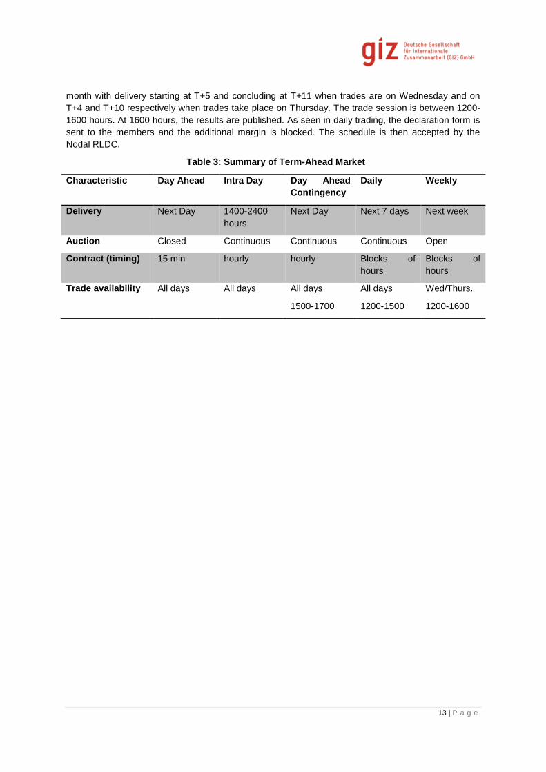
Table 3: Summary of Term-Ahead Market
Characteristic Day Ahead Intra Day Day Ahead
Contingency
Daily Weekly
Delivery Next Day 1400-2400
hours
Next Day Next 7 days Next week
Auction Closed Continuous Continuous Continuous Open
Contract (timing) 15 min hourly hourly Blocks of
hours
Blocks of
hours
Trade availability All days All days All days
1500-1700
All days
1200-1500
Wed/Thurs.
1200-1600

14 | P a g e
3 German Electricity Market
The set-up of the German electricity wholesale market and the developments to deal with the
integration of RES are described in this section. To integrate high shares of RES more flexibility is
needed in power systems. In a liberalized electricity market, the incentives to develop and operate
plants in a flexible way should be delivered by market signals. The design of wholesale electricity
markets therefor plays a key-role. Negative prices can signal a surplus of electricity better than a
zero-price, while low price-caps will give fewer incentives to players to operate when most needed.
Moreover, as forecasts improve significantly when calculated closer to the generation horizon, market
participants should be given an opportunity to manage their bids close to real-time. Intraday markets
could reduce the costs of balancing and help the integration of intermittent RES.
Figure 11: German electricity markets. (Fraunhofer IWES based on (Judith et al. 2011))
3.1 Regulatory Framework
The wholesale market in Germany is organized using balancing groups. Each group is a Balancing
Responsible Party (BRP) and can be responsible for the scheduling of generation and load, or traded

15 | P a g e
energy, or a combination of them. There are overall about 5000 BRPs in Germany including some
special BRPs used by grid operators summarizing renewable generation or grid losses.
In this section an introductive example is followed by a detailed description of the obligations and
market design regarding the balancing group concept. Please note: Power generation, transmission
and distribution, and retail is unbundled in Germany, with minor exemptions for very small utilities.
The imbalance settlement has some similarities to the settlement mechanisms used in India. But the
concept of reserve energy markets is (so far) not introduced in India.
In Germany all power producers and commercial consumers (i.e. distribution companies or industrial
companies) are obliged to forecast their energy consumption or production day-ahead and report their
quarter-hourly schedules to the responsible TSO. To do so, consumers and producers are organized
in balancing groups. Small power producers or consumers are able to cluster their activity in a
balancing group. In this case their total production and consumption is made accountable and
managed by one responsible representative. This is especially the case for distributed generation
such as renewable energies where hundreds and thousands of individual producers make up one
portfolio. Over- or under drawl in respect to the schedule is accounted by the TSO only balancing
group wise. Internal costs distribution is not regulated and settlement is done by the balancing group
members on an individual, contractual basis.
Activation of reserve power is only necessary if there is a net deviation in respect to the total schedule
of a control zone (sum of all balancing group schedules). Over- or under drawl of different balancing
groups may cancel each other out in case of opposite direction of deviation.
The imbalance price is calculated by dividing the sum of costs for reserve power activation by the total
reserve power delivered. If the control area is in a deficit situation (i.e. less production or more
consumption than scheduled) balancing groups which deviate from their schedules and contribute to
the situation (increase deficit) have to pay the imbalance price. Balancing groups which reduce the
deficit (more production or less consumption than scheduled) receive the imbalance price. In times of
surplus situation within the control zone it is the reverse case. This means one part of the total
balancing price charged is circulating between contributing and compensating balancing groups and
one part is used to refinance the activated control reserve.
3.2 Introductive example
To give a first impression of the balancing group concept the figure below describes the interaction of
two BRPs within the control area of a TSO for a fictive example of a deficit situation in a control zone
with two balancing groups and resulting money flows.

16 | P a g e
Figure 12 Interaction of two BRPs and a TSO in a control zone regarding scheduling and imbalance
settlement
Source: Fraunhofer IWES
BRPs are scheduling generation, consumption and exchange for every quarter hour in their own
responsibility. Also forecast of consumption and generation (including renewables) is the
responsibility of the BRP. The schedules have to be balanced. But the actual will deviate from
schedule. In the example the consumption of BRP1 is 10 MWh lower and the generation of BRP2 is
40 MWh lower than scheduled. The resulting imbalance of 30 MWh is handled by the TSO. For this
the TSO is contracting primary, secondary and tertiary reserves on the power reserve market
exchange. The costs for the contracted power are remunerated by the grid usage fees. The costs of
the actual utilized energy of secondary and tertiary reserves are remunerated by the BRP responsible
for the imbalance. (For primary reserves only power is contracted.)
In the example costs of 900 € occur for a specific quarter hour. Now these costs are divided by the
actual imbalance of the control zone which is 30 MWh leading to a reserve energy price of 30 €/MWh.
BRP1 is supporting the balancing of the TSO control zone with 10 MWh and receives 300 € from the
TSO. 40 MWh have to be utilized for the balancing of the schedule of BRP2 and for this the TSO
receives 1,200 € from BRP2. If surplus arises, like in the given example, this is used to cover the
power costs of the reserve contracting.
The imbalance price is supposed to incentivize balancing groups to comply with their schedules. As
the resulting control area situation at any moment of time is unknown and unpredictable for the
balancing group, the best strategy is to avoid deviation from schedule. However in the recent past,
additional rules have been introduced in order to increase the imbalance price if more than 80% of
procured control reserve has been activated. The imbalance price is than increased about 50%, but is
at least 100 EUR/MWh. Higher prices should increase the effort of a balancing group to predict
production or consumption adequately and avoid schedule deviations.
17 | P a g e
Beside the general balancing groups, a number of special balancing groups exist. The most important
types are:
Balancing group for residual deviations (DSOs):
o Is responsible for all imbalances within the DSO‘s grid which cannot be assigned to
any other balancing group due to quarter hour data which is not available
o Imbalance costs are split to grid usage fees
Balancing group for grid losses (DSOs and TSOs):
o Grid operators are responsible for buying energy to cover their grid losses; this is
done via this balancing group.
Balancing group for EEG-Trading (TSOs):
o The German TSOs are responsible to trade the energy that is subsidized due to the
EEG and that is not marketed by direct marketers
o Forecast is in the responsibility of the TSO
o They sell the energy only to the Spot Market
Balancing groups for direct marketing of renewables (renewable generators or aggregators):
o Forecast is in the responsibility of the generator or aggregator
Balancing groups of power exchange (power exchange):
o Traders at the power exchange do not trade directly which each other but via the
exchange
o Balancing groups of the power exchange are the counterparts of the trader’s
balancing groups
o As they are only trading balancing groups (they do not have any generation or
consumption points) they do not have any imbalances
3.3 Balancing groups
The commercial transfer of electrical energy in Germany is processed through balancing groups. A
balancing group accounts traded volumes and generation as well as consumption of measurement
points for every quarter of an hour. Every grid connection point has to be allocated to a balancing
group within a transmission system operator’s (TSO’s) control area (Electricity grid access regulation
Stromnetzzugangsverordnung (StromNZV) § 4 (3)). In a balancing group the power trades, electricity
generation and electricity consumption of a player or a group of players in the energy market are
pooled.
The balancing group contract is a standard contract which is prescribed by formal definitions of the
Federal Network Agency (Bundesnetzagentur 2011)3. It is concluded between the BRP and the
operator of the control area. The BRP needs balancing groups and according balancing group
contracts in every control area where he is trading or where he is responsible for measurement
points. In Germany, there are four control areas operated by the four TSOs TransnetBW, 50Hertz,
Tennet and Amprion.
A balancing group is created for diverse purposes by utilities, traders, large consumers, distribution
system operators or TSOs. A list of balancing groups is published regularly4. A distribution system
operator e.g. operates several balancing groups for the accounting of grid losses, the feed-in of
3 An English version of this contract can be found here:
http://www.tennet.eu/de/index.php?eID=pmkfdl&file=fileadmin%2Fdownloads%2FKunden%2FBNetzA-
BKC_englisch.pdf&ck=48c0a802ea08e09a09d442421b76ecf4&forcedl=1&pageid=324.
4 http://www.bdew.de/internet.nsf/id/DE_EIC-Codes-und-VNB-Bilanzkreise,
http://www.bdew.de/internet.nsf/id/205ED10B9209489EC1257D570040F5EC/$file/ENTSO-Code_EIC.pdf

18 | P a g e
renewable energy sources or the differences of household power purchase and consumption. In the
following the main aspects of the balancing group contract are explained5.
As a precondition for the conclusion of a balancing group contract for a balancing group with physical
grid connection the grid usage has to be agreed with the responsible distribution grid operator in
whose grid the connection points of the balancing group are located.
The balancing group contract enables both the feed-in and draw-off of electrical energy within the
TSO’s control area as well as the exchange of electrical energy with other balancing groups. The
exchange with other balancing groups can be a trade between two different companies within the
TSO's control area or a delivery to a balancing group of the same company in another TSO's control
area. The BRP has to inform the TSO immediately of the identity of the traders and suppliers who are
allocated to its balancing group. The BRP also has to make sure that it is reachable to the extent
required for a proper compliance with its contractual duties.
3.4 Market based balancing
As in India, power generators in Germany have different options for selling their production. These are
basically bilateral trade (over-the-counter, OTC) and trade over power exchange trade. Since the
liberalization in Germany the trade over the European Power Exchange has become more and more
important. While future products are used for price risk mitigation of the market participants short-term
markets have a direct impact on the physical balancing of demand and supply as power producer
decided upon their price signals weather production takes place or not. If prices are below the
marginal production costs power plants shut-down or decrease their power output and vice versa.
Today power trade is done on the day-ahead and intra-day market. The day-ahead auction ends at
12:00 p.m. (noon) and power for the following day (hours 0-24) can be traded in form of single hour or
block bids. In addition to this, it is possible to continuously trade for the next day in a separate auction.
Single hours and blocks can be traded continuously starting from 3 p.m. for the same or next day.
Quarterly-hour is possible starting from 4 p.m. This auction complements the quarter-hourly intra-day
trade which ends at 3 p.m. where power is exchanged for the next day in 96 intervals (hours 0-24).
At the moment the European Energy Exchange has three market regions (France, Germany/Austria
and Swiss). The market region Germany/Austria includes the area of the four German transmission
system operators (TSOs: Amprion GmbH, transpower GmbH, 50Hz, TransnetBW) and the Austrian
TSO (Austrian Power Grid). Compared to India the trading volume of the short-term markets in this
area is significant. In 2014 it has reached 263 TWh in the day-ahead market and 17 TWh hours in the
intra-day market. Trade on the day-ahead market was strongly influenced by the renewable
penetration which was around 150 TWh and has been sold to the power exchange. For comparison
the net electricity consumption in Germany in the same year has reached 512 TWh. Thus, around
51.4% of the physically delivered energy has been traded via the power exchange. In India in 2013-
2014 only 3% (30 TWh) of the generation has been sold via the power exchange as most of it is
bounded in long-term power purchase agreement (PPA) [EEX 2014, EMI 2014]. Consequently there
is a great difference between the role and impact of short-term markets in India and Germany.
However, trading volume at the power exchange in India has increased with a growth rate of 22% p.a.
in the last years.
5 The balancing group contract may be changed in the near future by the Federal Network Agency
(Bundesnetzagentur 2014a)

19 | P a g e
Price settlement at the EPEX spot market is based on the bids of market participants. The uniform
price results from the individual demand and supply curves resulting from these bids for each time
interval. The supply curve is influenced by the structure of the marginal production costs bidding
power plants. Real marginal production costs are not known, but can be estimated based on fuel and
plant type. A typical merit-order of all conventional power plants in Germany is depicted in Figure 13.
The marginal production costs especially depend on the fuel type and costs. Nuclear plants and
lignite plants are in general the cheapest plants followed by coal and natural gas power plants. Fuel
oil plants are rarely used due to very high costs. Combined heat and power (CHP) plants are able to
bid lower prices in the market as non-CHP plants of the same fuel type. This is because they can take
into account revenues from their heat production. Some plants with very high heat production
compared to their electricity production may even be able to bid with negative marginal costs. Power
plants with marginal costs below the current market price gain money. The uniform settlement price is
based on the marginal production costs of the most expensive power plant which is necessary to
cover the total demand.
Figure 13: Estimated marginal cost based merit-order for all German power plants
Source: Fraunhofer IWES
Every utility or large scale consumer can procure and every producer can sell its’ power in this
market. The market mechanism is thus responsible for balancing the demand and supply side on a
day-ahead or hour(s)-ahead base. Unexpected or unpredictable occurrences inflicting with load and
generation balance are settled in Germany by the control reserve of the system operator (explanation
in section .These are for example forecasting errors for RE production and load which are not known
before trading gate closure, power plant outages or unexpected unavailability. Accountability for not
complying with production and consumption schedules is enforced by the imbalance pricing
mechanism.
3.4.1 Scheduling
Schedules have to be transmitted from the BRP to the TSO until 14:30 of the previous day and have
to contain a balanced quarter hour performance for each quarter hour. Schedules within the German
control areas may be changed with minimum advance notice of one quarter hour to each quarter hour
0 10 20 30 40 50 60 70 80-100
-50
0
50
100
150
200
Installed capacity [GW]
Ma
rgin
al C
osts
[E
uro
/MW
h]
Merit-Order of capacity in Germany
Lignite
Coal
Natural Gas
Uran
Oil

20 | P a g e
of each day. Additionally, schedules within the control area of one TSO can be changed subsequently
until 4:00 of the following working day. Schedules can be transferred by File Transfer Protocol (FTP)
or via ISDN or by email. For the verification of the grid safety the TSO requires the schedule of every
power plant unit with a physical electrical capacity more than 100 MW until 14:30 at the previous day.
3.4.2 Spot market
Trading on the exchange spot market enables market participants to sell and buy electricity in a non-
discriminatory and anonymous environment and ensures the maximization of the social welfare
through merit-order dispatch (Jiang Wu et al.). Electricity can be traded in standardized contracts on a
day-ahead auction and a continuous intraday trading at the EPEX SPOT.
Energy traded in the power exchange markets accounted for 40% of the national electricity
consumption in the year 2013 with an increasing trend. The increase in the share can be explained
with the increase in generation from renewable energy sources and their need for day-ahead
settlement (EPEX SPOT 2014f).
Figure 14: Share of trading volume of national EPEX SPOT market in annual national (EPEX SPOT 2014f)
There are three exchange regulations, the code of conduct, the market rules and the operational
rules. This set of rules is agreed upon between the exchange operator and the market participants
and are uniformly applied to all market participants through contracts (EPEX SPOT 2014g).
The market rules organize the general exchange organization and operations procedures. They
contain information about the exchange operator, the purpose of the markets as well any fundamental
information about the exchange. The operational rules organize the details of the trading systems and
the traded products. The operational rules define e.g. tradable contracts, gate-closure-times, price
limits, order quantity, block types and further information to trade a product on the exchange. A fair
and transparent market operation is ensured by the code of conduct which regulates the behavior of
the exchange members. It also regulates the consequences when the rules are violated.
2009 2010 2011 2012 20130
10
20
30
40
50
Year
Perc
enta
ge
Percentage of annual consumpt ion

21 | P a g e
3.5 Product specifications
The sections below introduces to product details and the way of transaction and price determination
of the day-ahead auction market and the continuous intraday market at EPEX SPOT.
3.5.1 Day-ahead auctions
In a daily auction power contracts for every single hour of the next day are traded. An individual price
for every hour is determined in this auction. The sections below point out orders, product details and
the price determination.
3.5.2 Orders
Orders are submitted by exchange members via the ETS client. The orders placed in the trading
system need to fulfill specified conditions. Traders in the EPEX SPOT day-ahead market can place
single-contract orders or block orders. All orders and transactions are anonymous. The order book is
closed each day at noon, from when on orders cannot be changed and are binding. Single-contract
orders are only valid for one of the 24 hours and block orders for a defined combination of hours
(EPEX SPOT 2014b). Every hour that is intended to be traded individually needs an own single
contract order.
Single contract orders are placed as a monotonous demand curve with up to 256 price-quantity
combinations that limit the volume at a specific price. The curve is interpolated linearly between the
entered price-quantity combinations as in the following graph. It shows a generic offer curve with it’s
up to 256 price-quantity combinations.
Figure 15: Example of an individual offer curve at EPEX SPOT representing the up to 256 possible price-
quantity combinations
Buy volumes have no sign, sell volumes are signed with a minus. A monotonous curve means that an
increasing amount to buy must be entered with a decreasing price and an increasing amount to sell
must be entered with an increasing price. Prices are specified in steps of 0.1 EUR/MWh and volumes
in steps of 0.1 MW. Negative prices must be indicated with a minus. The entered prices must lie in-
P1
P2
P3
P256
P255
P254
Q1 Q2 Q3 Q254 Q255 Q256
…
22 | P a g e
between the minimum and the maximum price of the exchange market (table product details below)
(EPEX SPOT 2014b).
Different types of order can be placed in the market for different types of orders (EPEX SPOT 2014b):
Unlimited orders (single-contract or block) also called market orders or price-independent
orders. They must contain equal quantities for the minimum and the maximum order price
boundaries. These orders are fulfilled at any price.
Limited order (single-contract or block) have a price limit and are only executed if the market
prices matches the specified price or is better for the trader
All or none block orders are only executed if the market price for the entire volume matches
the specified price or is better for the trader. Otherwise the order would be rejected
Price-independent orders are placed e.g. by the TSO for the renewable energy feed-in in their own
balancing group6 or by market participants who aim towards a physical fulfillment of financial futures7
(EPEX SPOT 2014b),(EEX 2012).
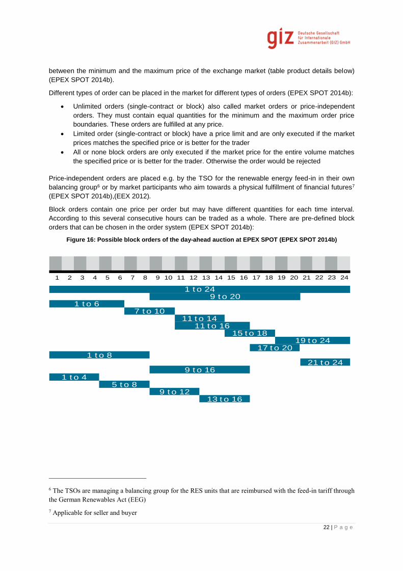
Block orders contain one price per order but may have different quantities for each time interval.
According to this several consecutive hours can be traded as a whole. There are pre-defined block
orders that can be chosen in the order system (EPEX SPOT 2014b):
Figure 16: Possible block orders of the day-ahead auction at EPEX SPOT (EPEX SPOT 2014b)
6 The TSOs are managing a balancing group for the RES units that are reimbursed with the feed-in tariff through
the German Renewables Act (EEG)
7 Applicable for seller and buyer
1 t o 249 t o 20
1 t o 67 t o 10
11 t o 1411 t o 16
15 t o 1819 t o 24
17 t o 201 t o 8
21 t o 249 t o 16
1 t o 45 t o 8
9 t o 1213 t o 16
1 3 4 5 6 72 8 10 11 12 13 149 15 17 18 19 20 2116 22 23 24
23 | P a g e
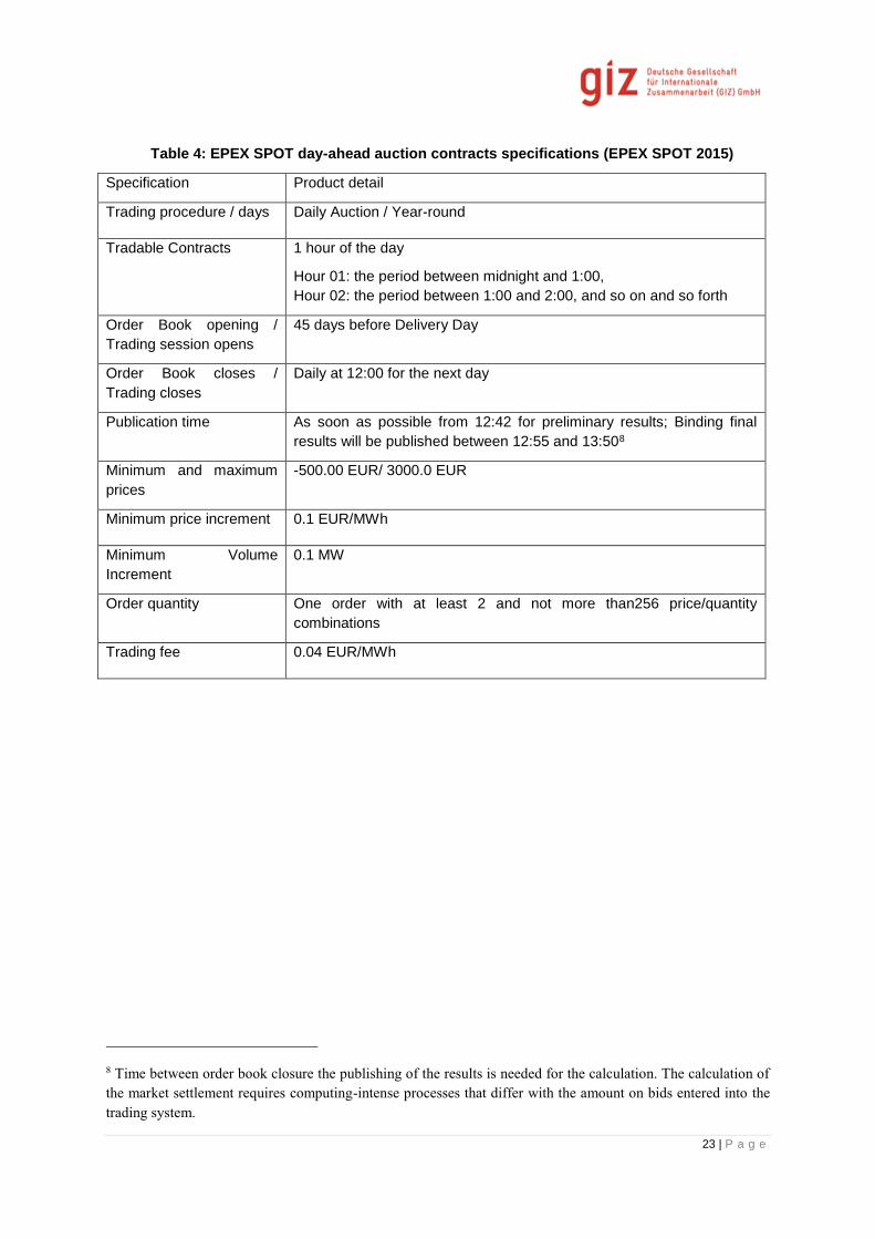
Table 4: EPEX SPOT day-ahead auction contracts specifications (EPEX SPOT 2015)
Specification Product detail
Trading procedure / days Daily Auction / Year-round
Tradable Contracts 1 hour of the day
Hour 01: the period between midnight and 1:00,
Hour 02: the period between 1:00 and 2:00, and so on and so forth
Order Book opening /
Trading session opens
45 days before Delivery Day
Order Book closes /
Trading closes
Daily at 12:00 for the next day
Publication time As soon as possible from 12:42 for preliminary results; Binding final
results will be published between 12:55 and 13:508
Minimum and maximum
prices
-500.00 EUR/ 3000.0 EUR
Minimum price increment 0.1 EUR/MWh
Minimum Volume
Increment
0.1 MW
Order quantity One order with at least 2 and not more than256 price/quantity
combinations
Trading fee 0.04 EUR/MWh
8 Time between order book closure the publishing of the results is needed for the calculation. The calculation of
the market settlement requires computing-intense processes that differ with the amount on bids entered into the
trading system.

24 | P a g e
3.5.3 Price determination
The orders are auctioned daily after the closure of the order book. The price is determined through
matching of the exchange members' aggregated supply and demand curves9 for each time interval
consisting of single orders and block orders. Block orders are only considered to be part of the
aggregated demand and supply curves if they can be executed completely. The price determined by
the trading system is the price at which the highest volume will be executed, the so-called market
clearing price. Afterwards, the price is determined considering the market-coupling with other spot
market auctions. The consideration of all constraints can lead to a different market price since the
aggregated demand and supply curves may differ from the initial solution. The market clearing price
will be set where both curves intersect. In this point the traded volume will be the highest, which is
also called quantity allocation. This entire process of price determination is called market clearing
(EPEX SPOT 2014b).
The market price and all order prices after price matching and quantity allocation are rounded to
0.01 EUR/MWh. For that purpose the exchange member's interest is assumed to be linear between
two price-quantity combinations. The matching algorithm also matches the prices with other market
areas, including network constraints on subsea cables. The matching algorithm executes sell orders
that are lower or equal to the market price and buy orders above or equal the market price. Orders
equal to the market price may be partially executed or not at all. If the matching algorithm does not
generate a valid market price (e.g. insufficient liquidity) a second auction is performed. This should
give the exchange members the chance to change their orders to improve the situation10. The results
of the joint German/Austrian market area shall be published and validated not later than 14:0011
(EPEX SPOT 2014b).
3.5.4 Post trading period
In the post trading period the market participants receive notice from the exchange operator about the
traded amounts. The exchange members are responsible for transferring the market results into
schedules for the TSO themselves. The exchange members forward the results to the corresponding
BRP for the creation of schedules. BRPs have to fill in the form for the schedule using the exchange
operator as a counterpart to balance positions. The energy exchange is a balancing group itself. The
traded amount on the exchange has to match the amounts in the exchange schedule of the BRP. If
the schedules are not balanced, they are rejected by the TSO, preventing imbalances prior to
production.
The BRP’s equilibrium of physical production, consumption and trading is covered by the balancing
group contract. Ultimately, trading on the exchange is a separate process to the obligations from the
balancing group contract.
9 Aggregated curves are the sum of all individual curves (demand or supply). Each one of them can consist of up
256 price-quantity combinations
10 The second auction is performed after the publishing of the results before the start of the intraday trading.
Second auctions for EPEX SPOT day-ahead markets are not happening often. In fact, the requirement of a
second auction is a sign of illiquidity of the markets which is not the case in the EPEX SPOT day-ahead market.
11 Including the second auction and before the start of the intraday trading.
25 | P a g e
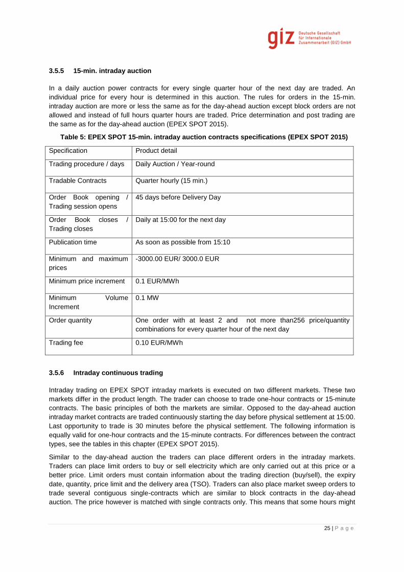
3.5.5 15-min. intraday auction
In a daily auction power contracts for every single quarter hour of the next day are traded. An
individual price for every hour is determined in this auction. The rules for orders in the 15-min.
intraday auction are more or less the same as for the day-ahead auction except block orders are not
allowed and instead of full hours quarter hours are traded. Price determination and post trading are
the same as for the day-ahead auction (EPEX SPOT 2015).
Table 5: EPEX SPOT 15-min. intraday auction contracts specifications (EPEX SPOT 2015)
Specification Product detail
Trading procedure / days Daily Auction / Year-round
Tradable Contracts Quarter hourly (15 min.)
Order Book opening /
Trading session opens
45 days before Delivery Day
Order Book closes /
Trading closes
Daily at 15:00 for the next day
Publication time As soon as possible from 15:10
Minimum and maximum
prices
-3000.00 EUR/ 3000.0 EUR
Minimum price increment 0.1 EUR/MWh
Minimum Volume
Increment
0.1 MW
Order quantity One order with at least 2 and not more than256 price/quantity
combinations for every quarter hour of the next day
Trading fee 0.10 EUR/MWh
3.5.6 Intraday continuous trading
Intraday trading on EPEX SPOT intraday markets is executed on two different markets. These two
markets differ in the product length. The trader can choose to trade one-hour contracts or 15-minute
contracts. The basic principles of both the markets are similar. Opposed to the day-ahead auction
intraday market contracts are traded continuously starting the day before physical settlement at 15:00.
Last opportunity to trade is 30 minutes before the physical settlement. The following information is
equally valid for one-hour contracts and the 15-minute contracts. For differences between the contract
types, see the tables in this chapter (EPEX SPOT 2015).
Similar to the day-ahead auction the traders can place different orders in the intraday markets.
Traders can place limit orders to buy or sell electricity which are only carried out at this price or a
better price. Limit orders must contain information about the trading direction (buy/sell), the expiry
date, quantity, price limit and the delivery area (TSO). Traders can also place market sweep orders to
trade several contiguous single-contracts which are similar to block contracts in the day-ahead
auction. The price however is matched with single contracts only. This means that some hours might

26 | P a g e
be executed and some are not12. Limit orders must contain information about the trading direction
(buy/sell), the expiry date, quantity, price limit and the delivery area (TSO). In addition to sweep
orders, pre-defined block orders can be placed (EPEX SPOT 2014b):
Block Base load covering hours 1 to 24
Block Peak load covering hours 9 to 20
The order book is open twenty-four hours a day throughout the year. EPEX SPOT however has the
right to close the order at any time. The information from the order book communicated from the
exchange to the exchange members for each contract during the trading session. This includes all
bids and ask limit order, details of the last trade, price, quantity and the time of execution. The single
contract orders (including sweep orders) are entered in a central open and anonymous order book.
Block order are handled in a separate order book. Orders are submitted electronically to the trading
system (EPEX SPOT 2014b).
Depending on the order’s price limit and quantity and on the order book configuration, any single
contract within the time range may not be executed since it cannot be matched with a counter
position. This means that contracts in some hours are executed where others are not. In addition to
this the executed volume may vary for each individual single contract since it can be possible that the
counter position does not have the matching volume. The orders placed in the trading system need to
fulfill specified conditions. Prices in limit orders must lie in-between the minimum and the maximum
price of the exchange market (see tables lower in this chapter). Negative prices must be indicated
with a “-“. Prices must be rounded to 0.01 EUR/MWh. Orders can be entered with the following
execution restrictions (EPEX SPOT 2014b):
“Immediate-or-cancel” (IOC): Either the order is immediately executed or automatically
cancelled. The order can be partially executed and any unexecuted quantity is cancelled. IOC
orders are not entered in the order book. Market sweep orders are orders with the restriction
IOC.
“Fill-or-kill” (FOK): The order is either immediately and entirely executed or cancelled in its
entirety. FOK orders are not entered in the order book.
“All-or-none” (AON): The order is executed completely or not at all. AON orders remain in the
order book until they are executed or cancelled.
orders can be entered with the following validity restrictions (EPEX SPOT 2014b):
“Good for session”: The order is deleted on the trading end date and time of the contract,
unless it is matched, deleted or deactivated beforehand
“Good till date”: The order is deleted on the date and time specified by the Exchange Member
when submitting the order, unless it is matched, deleted or deactivated beforehand.
“Iceberg” or hidden-quantity: An iceberg order is a large order, divided into several smaller
orders which are entered in the order book sequentially. The Exchange Member specifies the
total quantity and the initial quantity.
o The first order relates to the initial quantity
o The hidden quantity is then executed through a series of orders. Each order relates to
the same quantity as the initial quantity and there are as many orders as needed to
cover the hidden quantity. Each successive order is treated as a new order in terms
of priority in the order book. In case of quantity mismatch the event of an odd lot13
12 The block order would be executed fully or not at all (Fill-or-Kill condition)
13 This is the case when the bid from the iceberg order doesn’t have matching quantities on the opposite site

27 | P a g e
happens. This may lead to quantities of the last order being smaller than the initial
quantity.
After the submission of the orders to the trading system they are matched with other orders in the
order book. Matching takes places and orders are executed at the best price available in the system,
ensuring that order matching rules or priority rules are not violated.
3.6 Control energy or reserves for imbalances
The BRP needs to keep the feed-in and the purchase of energy in balance with the draw-off and the
sale of energy in every quarter of an hour. For this purpose, the BRP has to keep schedules for the
day-ahead planning. Balance deviations are only permitted if they are unpredictable. In case of an
unplanned power plant failure the BRP is released from these obligations for four quarter hours
including the quarter hour in which the failure occurs.
These remaining deviations from the schedules are compensated with balancing energy which is
provided by the TSO. The costs for balancing energy are given by a unique and common balancing
energy price (regelzonenübergreifender einheitlicher Bilanzausgleichsenergiepreis [reBAP]) which
applies symmetrically to the purchase and the delivery of balancing energy. The reBAP is calculated
based on the costs for activated control reserves in every quarter hour divided by the netted
imbalances of the four German control zones and then limited to the highest activated energy price
during this quarter hour and the average price of the continuous intraday trading for this quarter hour.
If more than 80 % of control reserves are activated an additional charge is added. Afterwards the
costs for the purchase of balancing energy for every balancing group are calculated by multiplying the
imbalance with the reBAP for every quarter hour. If the balancing group has received balancing
energy it has to pay the TSO for it. If the balancing group has supplied balancing energy the TSO has
to pay the balancing group.
The costs of this balancing energy are a risk that can be transferred to another balancing group. With
the permission of the other balancing group a subgroup can be created (StromNZV §4 (1)). The
account balance is than left at the parent balancing group that could be itself a subgroup of another
balancing group (StromNZV §4 (1)). The allocation of balancing groups can only be changed at each
1st day of a calendar month, 0:00, with a notification period of 10 working days.
3.6.1 Pricing, remuneration and settlement
Balancing reserves are contracted by the TSO on the reserve market. These markets are described in
this section. The technical specification of the reserve market products is given later together with a
description how reserve demand can be calculated. The markets can be distinguished between
primary control reserves, where only power is contracted, and secondary control reserves and minute
reserves, where power and energy are contracted. Market processes are made transparent by
regelleistung.net. Key information on pricing are summarized below.
In general, selected bidders are selected for provided control reserve only in accordance with the
merit order of capacity prices. Bids for the deployment (energy price bids) are only considered in case
where marginal bids have identical capacity prices. All selected bidders are paid according to their
individual capacity-price bid (pay-as-bid). With secondary control and minute reserves, provision of
control reserve capacity and deployed control energy are separately paid. Therefore, the bid of each
supplier has to specify a capacity price bid for provided reserves (paying the provision) as well as an
energy price bid for deployed reserves (paying a possible activation).
28 | P a g e
Referring to the tender of control reserve some special characteristics have to be considered:
In general and in accordance with the German regulator Bundesnetzagentur, TSOs may
define a minimum share of reserves (in German: Kernanteil) which have to be kept inside
each control area, i.e. a minimum of provision within this control area. Such minimum share
may be responsible for bids for the provision of control reserves within a control area being
considered as a matter of priority up to the amount of the minimum share regardless of the
bidding price.
Currently, however, such minimum shares are not required.
Remuneration of provided control reserves and of deployed control energy is accounted considering
the following principles;
The volumes to be accounted determine the level of remuneration (i.e. capacity provided
resp. energy delivered) as well as the prices the bidders indicate for each bid (pay-as-bid).
Remunerations are accounted for each delivery month, namely in the first weeks of the
following month.
The energy volumes relevant to the remuneration of deployed control energy of the qualities
of secondary control and minute reserves are calculated separately for each bid of each
bidder and for each quarter of an hour related to the delivery month. Then they are summed
up to monthly accounting amounts after being multiplied with the corresponding bid prices.
Costs for the deployed energy are born by the BRPs deviating from the schedule in direction of the
overall balance of the TSO control zone. For the imbalance settlement data of all generators and
consumers of a BRP are required. Larger generators or consumers are metered on a 15-min base.
Smaller ones are categorized using a standard load/ generation profile. The actual imbalance price is
published 42 days after the end of the month.
The data for the financial balancing settlement has to be provided according to the enactment BK6-
07-002 (MaBiS) of the Federal Network Agency.
The TSO will publish the reBAP not later than on the 20th working day after the delivery month and will
determine the balance deviations of the balancing groups from the 30th working day after the delivery
month based on the billing data available at the end of the 29th working day. The settlement of
balancing energy is made on a monthly basis, 42 working days after the delivery month, at the latest.
3.7 Cross-border trading
Cross-border trades are possible through market coupling between the market areas Germany,
France, Austria and Switzerland. However, special rules apply including restrictions of 15-minute
contracts only to countries with similar contracts or the consideration of different gate-closure times14
in the individual markets. On any other cross-border transmission capacity energy is traded explicitly.
The intraday trading system ComXerv facilitates the cross-border trading. Cross-border trading first
took place in December 2010 between Germany and France, the Austrian market joined in October
2012 and ultimately Switzerland joined in June 2013 (EPEX SPOT 2014e).
Market coupled trades do not require special actions by the participants. However, it is possible that
orders are cancelled because of unavailable transmission capacity. The transmission capacity that
was available at the time of order creation could be occupied at a later point. This can happen when a
different order is matched earlier or the transmission capacity is no longer available due to technical

29 | P a g e
constraints. Orders may be cancelled or reduced due to that reason. The event of an increase in
cross-border capacities and simultaneously sale order prices in the local order book being lower than
purchase order prices in the cross-border order book triggers an auction and stops continuous
trading. After this auction continuous trading is resumed (EPEX SPOT 2014b).
Based on a risk assessment and scoring of the clearing houses each single exchange member is
assigned a trading limit15. This limits the monetary value that can be traded by each exchange
member between two settlement days. Exchange members are not allowed to exceed their trade limit
(EPEX SPOT 2014b).
The following table shows the contract specification for the one hour intraday trading at the EPEX
SPOT:
Table 6: EPEX SPOT intraday continuous trading one hour contracts specifications (EPEX
SPOT 2014e)
Specification Product detail
Trading procedure / days Continuous / Year-round
Tradable Contracts 1 hour of the day
Hour 01: the period between midnight and 1:00
Hour 02: the period between 1:00 and 2:00, and so on and so forth
Order Book opening /
Trading session opens
24 hours a day
Hourly contracts for the next day open at 3:00
Order Book closes /
Trading closes
30 minutes before delivery
Publication time No publication time in continuous trading possible. Prices are
publicized continuously
Minimum and maximum
prices
-9999.99 EUR / 9999.99 EUR
Minimum price increment 0.01 EUR/MWh
Minimum Volume
Increment
0.1 MW
Order quantity Unlimited (with limit in daily monetary value stated by clearing house)
Trading fee 0.10 EUR/MWh
The fees for the participation on the German day-ahead auction and the correspondent intraday
segment are 10,000 EUR per annum. Transaction costs are 0.04 EUR/MWh. Annual technical fees
vary, depending on the technical implementation between 2,000 EUR and 8,000 EUR. Each
15 Information on the scoring system and the results are subject to individual contracts between the clearing
house and the trading member and therefore are confidential.

30 | P a g e
cancelled order will be charged with 50 EUR per order (day-ahead and intraday) (EPEX SPOT
2014c).
3.8 Market coupling
Figure 17: Principles of price convergence in coupled electricity markets (PCR 2014b)
The graph above shows the principles of market coupling. The downward curve is the demand curve
and the upward curve is the supply curve. The intersection of the blue lines on the left graph at the
price PA and the quantity QA is the market equilibrium in the local market (market A). The intersection
of the blue lines on the right side shows the market equilibrium in the neighboring market (market B)
with the equilibrium price PB and the equilibrium quantity QB. Both sides show market prices in
isolated markets. Market A has a lower price than market B. If both markets are coupled and the
merit-order list are joined the demand curve in market A shifts upwards since the cumulated demand
curve from both markets increases the demand. This is due to the fact that market B has access to
lower electricity prices now. In the same time the supply curve shifts downwards in market B since it is
less beneficial to produce at lower prices. This increases the electricity prices in market A. In
conclusion one can say that market coupling harmonizes market prices and therefore encourages the
most efficient unit commitment (den Ouden, Jean Verseille 1/6/2011). The resulting gain in social
welfare is published by the EPEX SPOT for CWE region (EPEX SPOT 2014a).
In order to increase the social welfare and efficiency of markets it is necessary to incorporate as many
participants in the market as possible. Ideally all market participants would be trading on the same
market platform. Due to grid constraints and other barriers, markets are locally segmented though.
These segmented markets can be brought together by the means of market coupling. Market coupling
optimizes the allocation process of cross-border capacities. Exchange members do not have to care
about transmission capacity. It is also called implicit trading. The available transmission capacity is
determined by the TSO through grid calculations. This happens for the annual and month-by-month
basis using seasonal values and for the day-ahead and intraday capacities on a flow-based grid
calculation (EPEX SPOT 2013). The different exchanges who participate in the market coupling use
the available cross-border transmission capacity. Supply and demand curves of the different market
areas can be aggregated. Depending on the available transmission capacity the price difference is
minimized. This means that prices increase in the market areas with the low prices and prices
31 | P a g e
decrease in the market areas with high prices. Bottlenecks will lead to market splitting and merit order
lists in the different market to be different, which changes the order of dispatch of power plants.
Since February 4, 2014 there is a market coupling of northern west Europe (NWE). NWE replaces
former market couplings such as the CWE coupling and the coupling of CWE to the Nordic region via
Interim Tight Volume Coupling (ITVC). NWE is based on the initiative Price Coupling of Regions
(PCR) of the power exchanges APX, Belpex, EPEX SPOT, GME, Nord Pool Spot, OMIE and OTE.
NWE covers the countries:
Nordic region: Denmark, Finland, Norway, Sweden
Great Britain
CWE region: Belgium, France, Germany, Luxemburg, Netherlands
Baltic states and Poland are not directly involved but they are coupled to the Nordic market via
NordPoolSpot16 (NPS) (EPEX SPOT 2014d). Furthermore, power markets of Portugal, Spain and
France (SWE) are coupled by applying the PCR solution hence keeping the explicit trading
algorithm17. Explicit trading means that energy and transmission capacities are allocated separately
(CASC.EU 2014c). The long term goal is a market coupling of the entire European Union.
The PCR solution has been developed by European Power Exchanges to provide a single algorithm
and harmonized operational procedures for efficient price calculation and use of European cross-
border transmission capacity, calculated and offered to the market in a coordinated way by TSOs
(Beckman 2014). The NWE market coupling is realized by the implementation of the algorithm
"Euphemia" (EU + Pan-European Hybrid Electricity Market Integration Algorithm) to calculate market
prices, net positions and flows on interconnectors between market areas (PCR 2014a, 2014b). The
algorithm is applied to couple the day-ahead spot market of power exchanges.
3.8.1 Cross border capacity allocation
In addition to trade on the spot market with market coupling applied, one can trade cross-border
transmission capacities. These cross-border transmission capacities are allocated with different time
horizons. The transmission capacity can be acquired specifically to transmit power from one country
to another without having to rely on power exchanges. It enables traders to access local markets at
the given local price at the exchange. One can sell, for example, electricity on the French market with
a unit which is connected to the German grid. This electricity will be sold on the French market, even
in the case of congestion in the spot market. The cross-border transmission capacity can be acquired
at CASC.EU, which is a subsidiary of the involved TSOs on a European level. For Germany the TSOs
TenneT, Amprion and TransnetBW are shareholders of CASC.EU. The capacities can be acquired for
the time span of an entire year of for a whole month and if available, as well on a daily basis
(CASC.EU 2014a).
The company that acquired the transmission capacity is the holder of the capacity. It has the right to
nominate the transmission capacity on a day-to-day base. This means it can announce the usage of
the capacity between 0 and full capacity. If the capacity holder does not wish to use the capacity
entirely or not at all it can be sold in different ways. A first option is the return to CASC.EU for a whole
16 NPS is the market operator in the ENTSO-E Regional Group Nordic (Eastern Denmark, Finland, Norway and Sweden)
equivalent to EPEX SPOT.
17 The PCR solution couples different market coupled areas. “PCR will operate without offering capacity at the French-Spanish
border to the price coupling, so the daily explicit auction on this border will be maintained as it is today. The final step in SWE
integration will take place when all legal, regulatory and IT conditions are satisfied. The daily explicit auctions will then stop and
PCR will then offer the implicit day-ahead allocation for the French-Spanish border.” (CASC.EU 2014c)

32 | P a g e
month. The capacity holder then is reimbursed with the price for the capacity from the monthly
contract. Second option is the transfer of capacity to a different company. Prices and conditions are
agreed upon via OTC contracts. Third option is keeping the capacity and making it available for
market coupling. The reimbursement is calculated as the price difference between the two markets
after market coupling times the unused capacity. (Pergel 9/25/2014)
Compensation = unused capacity * price spread
Interconnectors without market coupling capacities are tendered through CASC.EU also for the day-
ahead and intraday case.
CASC.EU describes itself at the central auction office for cross-border transmission capacity for
Central Western Europe, the borders of Italy, Switzerland, Norway and Denmark. The trading on the
platform includes secondary markets. The initial auction session is a trade between the respective
TSOs and the customers. On the secondary market transmission capacities are traded between
different customers. This means that already acquired capacity can be sold to other market
participants (CASC.EU 2014a).
Access to CASC.EU can be gained through the website. Each category of cross-border transmission
capacities has to be applied for separately. The different regions for available transmission capacities
are Central Western Europe (CWE consisting of Belgium, France, Germany, Luxembourg and the
Netherlands) CWE (additionally consisting of Spain and Portugal), Swiss borders, Danish borders
(internal/external) and the France-Spain border. Intraday auctions have between any of these
countries has to be applied separately. The admission process in general includes the filling of forms
for the different interconnectors. After admission by CASC.EU access to the trading system is granted
and traders can be trained for the participation. All admission criteria are accessible at (CASC.EU
2014b).
3.9 Network tariffs
Network costs are typically recovered via a transmission tariff that can be paid by consumers or
generators. Tariffs can be split in a capacity and an energy charge. As networks are in general
understood as natural monopolies, tariffs are mostly regulated by a governmental body or regulating
authority.
Tariffs are should designed such that they do not hinder the development of renewables. There is
however one characteristic that could be crucial for variable RES integration: whether charges are
proportional to the energy consumed, or to the maximum capacity.
Due to their low capacity factor, variable RES are affected negatively by charges based on maximum
capacity. Also conventional power plants with a higher contribution to balancing and frequency
regulation services will be affected.
In Germany, generators (RES as non-RES) do not pay any injection tariffs. Thus there is no
advantage in respect to network tariffs for controllable over not-controllable injection. A drawback can
emerge on the consumption side.
The costs of reinforcing the network are covered by the network operators and included in the
transmission and distribution tariffs paid by network users. For consumption based network tariffs, this
can lead to a proportional higher burden for energy consumption in grid areas, where generation
shows a significant surplus over demand and network costs are driven by generation capacity. There

33 | P a g e
are grid areas in Germany, especially in the North-East, with very high wind capacity installed and
relatively low demand. A discussion is ongoing, how much network tariffs for end user consumption
are getting in proportionate and how to mitigate this effect.
In India there is a capacity based network tariff for inter-state power transfer. This tariff should be
developed to foster integration of RES, make use of combinations of different generation sources in
different states and to foster flexible use of power plants.
3.10 Renewable Energies within the set-up of regulation and mechanisms
3.10.1 Funding and refinancing
Germany has introduced RE by establishing a technology specific feed-in tariff which guarantees a
fixed price for each per kilowatt-hour produced for 20 year of operation (funding). For RE generators
operating under the FiT scheme, the TSOs have the responsibility to sell the electricity production on
the short-term market (refinancing). The difference between the total market revenue and the total
payment of FiTs to the generators is covered by the final consumers which are obliged to pay a fixed
surcharge on every kilowatt-hour of consumed electricity (refinancing).
In 2012 a market premia has been introduced on a voluntary base within the direct marketing
scheme. This scheme allows new market players (aggregators beside the TSOs) to market RE
production on the short-term-market. In addition to this revenue a market premia compensates for the
difference between the technology specific reference market price and the “applicable value” which is
basically the FiT price. The reference price, and thus the market premia, is calculated once a month in
order to account for changes of the spot-market price. This way a very predictable income is
guaranteed as an income to the generator. The cost for the market premia is analogously paid by the
final end consumer in form of the fixed charge applied to electricity consumption.
Direct marketing under the market premia became mandatory for plants commissioned after the
01.08.2015. However, small plants below 500 kW of installed capacity are exempted. This threshold
will decrease down to 100 kW in 2016. Then only small PV power plants are effectively eligible for the
FiT scheme and marketing via the TSO.
Figure 18: Concept of direct marketing & refinancing RE

34 | P a g e
3.10.2 Marketing of RE and conformity with balancing group concept
Direct marketing is typically done by private companies which buy the electricity generation from
many different distributed RE generators, aggregate it and sell it to the market. These companies as
well as the TSO which is marketing RE generators under the FiT scheme have to account the
generation within a balancing group. All generation needs to be forecasted for the next day and
scheduled accordingly complying with existing balancing group rules. According to the rules a
demand schedule has to be presented which exactly matches the generation schedule in every 15-
min interval. This can be either the projected demand of contracted consumers (in case the direct
marketing company is also working as a DISCOM) or the demand which has been contracted by
trading and selling the generation at the power exchange (valid in the case of the TSO or direct
marketing companies which do trading at the power exchange). Actual deviations at the time of
physical delivery between scheduled demand and generation are penalized and an imbalance price
has to be paid for every kWh of deviation. Deviations may occur especially due to forecast errors or
technical, unpredicted non-availabilities of power plants.
All traders of RE have the possibility to minimize their deviations by forecasting their generation
additionally as close as to trading gate closure. Thus, given i.e. a two hours-ahead forecast with
higher accuracy than the day-ahead forecast allows the trader to set its power position straight and
sell or buy electricity at the intra-day-market and correct for over- or underestimation of power supply
at the time of physical delivery. This way the cost of imbalance pricing can be minimized.
The remaining imbalance pricing costs is finally paid by the operator of the RE generators. However,
settlement of this cost distribution is left to bilateral agreements between RE generators and the direct
marketing company. In the case of the FiT scheme the TSO socializes these costs towards the final
consumer. Compared to the general costs of funding and refinancing RE these costs are very low in
Germany and can be estimated to be around 0.2 ct/kWh while the average costs per kWh of RE in
Germany is 16.25 ct/kWh (average over all technologies and all existing plants). Due to economies of
scale in marketing and forecasting of RE as well as organization management most direct marketing
companies have portfolio with more than 1000 MW of RE capacity. The largest company manages a
portfolio of 8700 MW.

35 | P a g e
Figure 19: Portfolio size of 30 selected direct marketing companies
3.10.3 Impact on short-term markets and consequences
Marketing RE on short-term markets has significantly increased the trading volume in the past years.
Today roughly 50% of the total electricity consumption is traded on the day-ahead spot market of the
European Power Exchange (German/Austrian price zone). High RE production directly impacts the
price development at the spot market. The following figure shows the electricity production by source
and the resulting price at the intra-day and day-ahead markets. If renewable production is high prices
tend to be low – especially during times of low demand. If large amounts of conventional units are
needed prices tend to be high.
The reason being is that markets are working on a marginal cost base. The uniform price for all
market participants id determined by matching the supply and demand curves in every hour. An
illustrative example of the pricing mechanism is depicted in
Figure 21. In the above graph a situation with no feed-in from RE is displayed. The dotted red line
indicates the present demand (60 GW) and the resulting price given the marginal costs of the
displayed conventional capacity (nuclear, lignite, coal, oil)18. In the lower graph the same situation is
displayed with around 10 GW of generation from RE. As RE have no fuel costs and thus very low
marginal or operating costs and in addition receive a market premia in Germany, they are able to bid
with very low or negative prices in the market. This way the merit-order is shifting and the same
18 The graph display illustrative costs derived from fuel costs and plant specific parameters (i.e. efficiency). For combined cycle
plants the marginal costs are reduced by the income from heat generation and sale. This additional income may lead to the
willingsness to accept negative prices. In general real marginal costs of plants are not known and can only be estimated.
0
1,000
2,000
3,000
4,000
5,000
6,000
7,000
8,000
9,000
10,000St
atkr
aft
Mar
kets
Gm
bH
Dan
ske
Co
mm
od
itie
s…
ene
rgy2
mar
ket
Gm
bH
Gru
nd
grü
n E
ne
rgie
Gm
bH
Tria
nel
Gm
bH
/Ges
y
Vat
ten
fall
Euro
pe
Sale
s G
mb
H
Cle
an E
ne
rgy
Sou
rcin
g
MV
V E
ne
rgie
AG
WE²
Gm
bH
Nea
s En
erg
y A
IS
Eon
En
ergi
e D
eu
tsch
lan
d
Nex
t K
raft
we
rke
Gm
bH
RW
E D
eu
tsch
lan
d A
G
Axp
o D
eu
tsch
lan
d G
mb
H
EnB
W T
rad
ing
Gm
bH
Ener
con
/Qu
adra
En
erg
y
Mar
k-E
AG
RW
E In
no
gy G
mb
H
in.p
ow
er
Gm
bH
Ko
M-S
olu
tio
n G
mb
H
Nat
urs
tro
m A
G
Iber
dro
la G
ener
atio
n
Ste
ag N
ew
En
ergi
es G
mb
H
envi
a M
itte
lde
uts
che
En
ergi
e…
GD
GE
Gen
oss
ensc
haf
t…
Pfa
lzw
erke
AG
Mai
no
va A
G
bad
eno
va G
mb
H &
Co
. KG
Ener
gie
die
nst
Ho
ldin
g A
G
Allg
äue
r Ü
ber
lan
dw
erk
Gm
bH
Size
of
RE
po
rtfo
lio in
MW

36 | P a g e
demand can be catered with less conventional units and thus, lower costs. The resulting (illustrative)
price is around 38 EUR/MWh instead of 50 EUR/MWh. This price reducing effect or RE is called
merit-order effect and varies i.e. according to RE penetration level, actual demand and price
sensitivity of demand, power plants available and bidding.
The resulting market price on the day-ahead market is uniform and thus valid for all bidders. Units
with lower marginal costs can realize an operating margin.

37 | P a g e
Figure 20: Electricity production by source and price development at EPEX spot markets

38 | P a g e
Figure 21: Illustrative example: Marginal cost pricing mechanism and merit-order effect of RE
Negative prices (electricity consumer receives money) on the day-ahead spot market in Germany
occurred in 64 hours in the year 2014. They indicate a situation of oversupply. Today they are caused
by conventional generation not backing down in times of high RE supply. Power plant may not be
willing to reduce their power to various reasons. Among these are:
shut-down or start-up is more expensive than accepting negative prices for a few hours
power plants also provide ancillary services (control reserve) and stay therefore on bar
combined heat and power plants have to fulfill their heat delivery obligations
Power plants which are inflexible due to these reasons are also referred to as conventional must-run
socket. In future the aim is to reduce this amount of capacity (i.e. by integrating heat storage into
CHP-units, providing control reserve by other means i.e. batteries, power-to-heat plants).
All in all the merit-order effect of RE – especially of PV reducing prices during peak times (i.e. at
noon) – has brought down spot market prices significantly down (Figure 22). The annual average
price in 2014 has been reduced about 26% compared to 2010. Although other effects (i.e. change in
fuel prices and resulting fuel switch from gas to coal) have influenced the price level as well, RE
market integration has been the major driving force. As conventional power plants in Germany are not
Page 18
Example of merit-Order without renewable energies
XXX11/06/2015
0 10 20 30 40 50 60 70 80-100
-50
0
50
100
150
200
Installed capacity [GW]
Ma
rgin
al C
osts
[E
uro
/MW
h]
Merit-Order of capacity in Germany
Lignite
Coal
Natural Gas
Uran
Oil
Page 19
Example of merit-Order with renewable energies
XXX11/06/2015
0 10 20 30 40 50 60 70 80-100
-50
0
50
100
150
200
Installed capacity [GW]
Ma
rgin
al C
osts
[E
uro
/MW
h]
Merit-Order of capacity in Germany
Lignite
Coal
Natural Gas
Uran
Oil
0 10 20 30 40 50 60 70 80-100
-50
0
50
100
150
200
Installed capacity [GW]
Ma
rgin
al C
osts
[E
uro
/MW
h]
Merit-Order of capacity in Germany
Lignite
Coal
Natural Gas
Uran
Oil
Renewable Injection of 10 GW
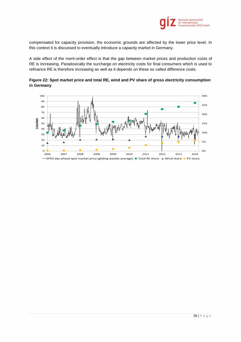
39 | P a g e
compensated for capacity provision, the economic grounds are affected by the lower price level. In
this context it is discussed to eventually introduce a capacity market in Germany.
A side effect of the merit-order effect is that the gap between market prices and production costs of
RE is increasing. Paradoxically the surcharge on electricity costs for final consumers which is used to
refinance RE is therefore increasing as well as it depends on these so called difference costs.
Figure 22: Spot market price and total RE, wind and PV share of gross electricity consumption
in Germany
0%
5%
10%
15%
20%
25%
30%
0
10
20
30
40
50
60
70
80
90
100
2006 2007 2008 2008 2009 2010 2011 2012 2013 2014
EUR/
MW
h
EPEX day-ahead spot market price (gliding weekly average) Total RE share Wind share PV share

40 | P a g e
4 Ancillary Services (AS)
For the operation of electrical supply systems a bundle of services have to be provided and system
inherent characteristics have to be considered to ensure the reliability and the quality of the power
delivered. The figure below gives a survey of important characteristics and services.
Figure 23: Survey of important system characteristics and services
Source: Fraunhofer IWES
System characteristics are inherent and composed of the individual characteristics of all generators
and loads connected to the system as well as the grid lines, transformers, etc. Ancillary services can
be delivered by generators, loads or dedicated devices like FACTS, but will be activated automatically
or by request of the system operator. For the operational services the grid operator has to take the
responsibility.
The impact of intermittent RES like wind and solar power on these services is two-fold. Firstly, due to
their characteristics including uncertainties in predictability, a large penetration of intermittent RES will
impact upon the need for these services. Secondly, intermittent RES will change the system
characteristics and are not (or not yet) able to provide some of the ancillary services. Other services
could be delivered by RES but the contribution from RES may not yet be requested. The table below
summarizes stake holders and their functions in ancillary services market of Germany.
System Operation
System Characteristics
Inertia
Self-regulation Effects
Short Circuit Capacity
Ancillary Services
FrequencyControl
FrequencyContainment
FrequencyRestoration
Reserve Replacement
Voltage Control
Dynamic (Fault-ride-trough)
Static
System Restoration
Black Start Capability
House Load Operation
Grid Energizing Capability
Operational Services
System Coordination/
Dispatch
System Control
Data Acquisition
Compensation of Grid Losses

41 | P a g e
Table 7: Classification of ancillary and operational services in Germany
Ancillary
service
Frequency control Voltage control System restoration System control
Objective Maintenance of the
frequency in the permitted
range
Maintenance of the
voltage in the per-
mitted range
Restriction of the
voltage drop in the
event of a short
circuit
System restoration
after faults
Coordination of the
grid and system
operations
Products/
Measures
Instantaneous re-serve
Balancing energy
Flexible loads
Frequency-dependent
load shedding
Active power reduction on
excessive/insufficient
frequency
Provision of
reactive power
Voltage-related re-
dispatch
Voltage-related
load shedding
Provision of short
circuit power
Voltage regulation
Coordinated
commissioning of
feeders and sub-
grids with loads
Black start
capability of
generators
Grid analysis,
monitoring
Congestion
management
Feed-in
management of
RES
Coordination of the
provision of ancillary
services across grid
levels
Current
providers
(selection)
Conventional power plants
Flexible controllable loads
Balancing energy pools
(including RE systems and
large-scale batteries)
Conventional
power plants
Operating
equipment (e.g.
reactive power
compensator,
FACT)
RE systems
Black start
capable thermal
power plants
Pumped-storage
power plants
Network control
units directing
operating equipment
and conventional
power plants
For the integration of high shares of RES firstly the ancillary services frequency and voltage control
have to be considered and will be described in more detail in the following sections.
4.1 Development of joint operational procedures
For the European power system the entso-e System Operations Committee (SOC) develops
recommendations for harmonized operation procedures.
The SOC ensures a high standard of operability, reliability and security of the European electricity
transmission systems within the framework of liberalized energy markets. The SOC consists of
representatives from all TSOs. (ENTSO-E, 2015)The Committee provides proposals for
harmonization of operational standards (network codes and rules) on the pan-European level and
promotes operational coherence among regions. It contributes to ensure compatibility between
system operation, market solutions and system development issues.

42 | P a g e
Table 8: SOC and Regional group activities
SOC Activities: Regional Group Activities:
Developing European operational
standards
Protecting critical systems
Developing and maintaining the
Electronic Highway
Developing a functional model
Defining a methodology for dealing with
operational reserves
Classification and follow up of incidents
Promotion and enhancement of coordinated
system operation and services.
Enhancing and developing operational
processes
Investigation of frequency deviations;
Enhancement and maintaining of network
models and forecast tools
Observing and enhancing the system
performance and dynamic behavior;
Compliance monitoring and enforcement;
and
Integrating internal and interconnecting
external systems.
The above planning and control structure of entso-e is a solution the solution that encompasses fair
operations in an international system.
India has multiple states with conflicting interests when referring to energy. It is recommended that an
independent body be formed with representation from every load dispatch center. It is proposed that
this committee be given powers and resources via legislation to execute functions as mentioned
above.
4.2 Organizational Implementation of the Frequency Control
In Germany and Europe, the frequency management is done by providing primary, secondary and
tertiary control. Primary control keeps frequency deviations within a narrow band, secondary control
restores the frequency to the set point of 50 Hz and the tertiary reserve replaces the secondary
control and sustains the frequency. In the following sections, the processes for provision of primary
and secondary reserve are described.
4.2.1 Control activities
The framework of the load-frequency-control (LFC) process is based on both a dynamic and a
geographic hierarchy. The dynamic hierarchy follows a three step approach:
1) Frequency Containment Reserve (FCR) or primary control
The Frequency Containment Process stabilizes the frequency after the disturbance at a steady-state
value within the permissible Maximum Steady-State Frequency Deviation by a joint action of FCR
within the whole Synchronous Area. The reserve is automatically activated by frequency
measurement.
2) Frequency Restoration Reserve (FRR) or secondary control
The Frequency Restoration Process controls the frequency towards its set point value by activation of
FRR and replaces the activated FCR. The Frequency Restoration Process is triggered by the
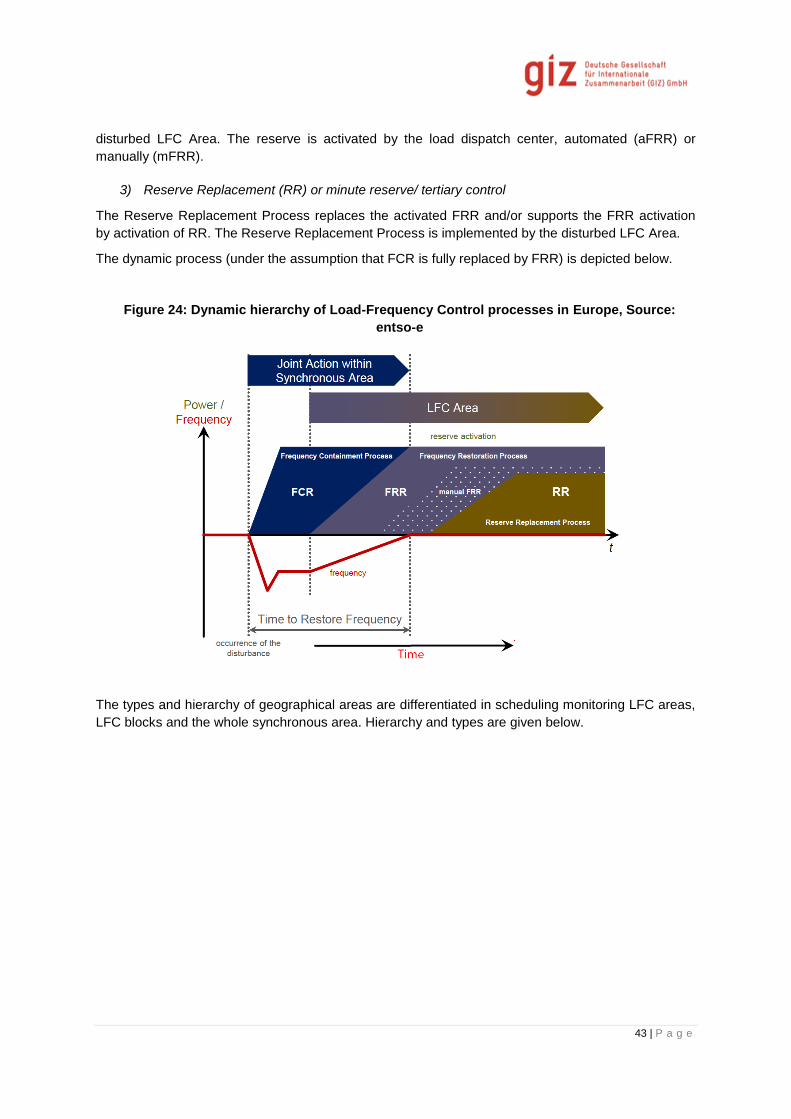
43 | P a g e
disturbed LFC Area. The reserve is activated by the load dispatch center, automated (aFRR) or
manually (mFRR).
3) Reserve Replacement (RR) or minute reserve/ tertiary control
The Reserve Replacement Process replaces the activated FRR and/or supports the FRR activation
by activation of RR. The Reserve Replacement Process is implemented by the disturbed LFC Area.
The dynamic process (under the assumption that FCR is fully replaced by FRR) is depicted below.
Figure 24: Dynamic hierarchy of Load-Frequency Control processes in Europe, Source:
entso-e
The types and hierarchy of geographical areas are differentiated in scheduling monitoring LFC areas,
LFC blocks and the whole synchronous area. Hierarchy and types are given below.

44 | P a g e
Figure 25: Types and hierarchy of geographical areas in Load-Frequency Control processes
in Europe and a possible configuration of a synchronous area, Source: entso-e
Currently the following status applies in Europe:
GB, IRE and NE currently consist of exactly one LFC Block and LFC Area.
Continental Europe (CE) currently consists of many LFC Blocks as shown below. Most of
these LFC Blocks consist of one LFC Area, such as LFC Blocks operated by RTE, ELIA,
TenneT NL, and Terna but there are also several examples of LFC Blocks that consist of
more than one LFC Area such as
o The LFC Block of Spain and Portugal with LFC Areas operated by REN and REE;
and
o The German LFC Block with four LFC Areas operated by 50HzT, Amprion, TenneT
Germany (including Energinet.dk) and TransnetBW.
Figure 26: Current status of Synchronous Areas, LFC Blocks and LFC Areas in Europe,
Source: entso-e

45 | P a g e
4.2.1.1 Activation of FCR or primary control
The FCR is activated by a joint action of FCR providing units and groups within the whole
synchronous area with respect to the frequency deviation. FCR is not a directed activity but triggered
by decentralized frequency measurements. The overall behavior shall follow two principles:
The overall FCR activation is characterized by a monotonically decreasing function of the
Frequency Deviation.
The total FCR capacity shall be activated at the maximum steady-state frequency deviation.
For conventional power plants this is achieved by implementation of turbine governors and the
parameterization of the FGMO.
4.2.1.2 Activation of FRR or secondary control
The FRR is directed by the TSO and triggered automatically or partly manually. For the requirements
of the necessary SCADA and communication system the general layout of the REMCs as proposed in
WP1 report “Report on Assessment of existing SCADA/EMS Control Centers Telecommunication
Infrastructure and Conceptual Design of new REMCs” should be followed.
4.2.2 Assessment of balancing needs and level of responsibility
To see the influence of primary control and of the penetration level of RES a frequency response
model was developed and simulations were carried out.
4.2.2.1 Frequency response modeling
To provide a more detailed view on balancing capability a suited model is set up for investigations of
frequency behavior in dependence of active power changes and the influence of primary control. For
this purpose a balance point model is used.
The frequency behavior in the balance point model is described by the following parameters of
The System
Inertia H (MWs)
The load
Frequency dependence of the load D (MW/Hz)
The generation
Conventional power plants
Capacity in operation
Governor operation mode
RE
Share of actual power generation
Operation mode (e.g. frequency dependent curtailment)
Thus the effects of active power changes on frequency could be analyzed. The detailed grid topology,
line congestions, etc. is not considered.
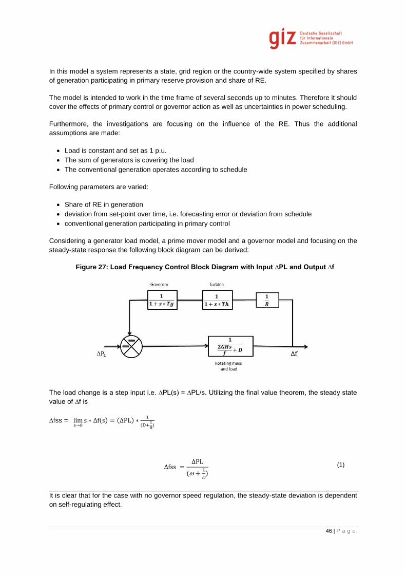
46 | P a g e
In this model a system represents a state, grid region or the country-wide system specified by shares
of generation participating in primary reserve provision and share of RE.
The model is intended to work in the time frame of several seconds up to minutes. Therefore it should
cover the effects of primary control or governor action as well as uncertainties in power scheduling.
Furthermore, the investigations are focusing on the influence of the RE. Thus the additional
assumptions are made:
Load is constant and set as 1 p.u.
The sum of generators is covering the load
The conventional generation operates according to schedule
Following parameters are varied:
Share of RE in generation
deviation from set-point over time, i.e. forecasting error or deviation from schedule
conventional generation participating in primary control
Considering a generator load model, a prime mover model and a governor model and focusing on the
steady-state response the following block diagram can be derived:
Figure 27: Load Frequency Control Block Diagram with Input ∆PL and Output ∆f
The load change is a step input i.e. ∆PL(s) = ∆PL/s. Utilizing the final value theorem, the steady state
value of ∆f is
∆fss = lims→0
s ∗ ∆f(s) = (∆PL) ∗1
(D+1
R)
∆fss =∆PL
( +1
) (1)
It is clear that for the case with no governor speed regulation, the steady-state deviation is dependent
on self-regulating effect.

47 | P a g e
∆fss =∆PL
(2)
The detailed description of the model development is given in the annex 2
4.2.2.2 Assessment of balancing needs
In this section, studies have been carried out to understand the steady state frequency deviation
without considering governor speed regulation and with considering governor speed regulation
initially; the case study is performed without considering the governor speed regulation. The steady
state frequency deviation mainly depends on:
Difference in power due to the deviation from the schedule ∆PL
Self-regulating effect D
∆PL consists of the following parameters:
Share of RE in generation
Deviation from set-point over time
In order to understand the impact on steady-state frequency deviation, schedule deviation is varied in
percentage with self-regulating effect ‘D’ is assumed as 1 (i.e. 1% change in frequency would cause
1% change in load). The different curves are plotted in the same graph for different amount of share
in the RE. The figure shown below gives steady-state frequency deviation for different share of RE
without considering speed regulation.
Figure 28: Steady state frequency deviation for different shares of RE - no speed regulation
Figure above shows that the steady state frequency deviation would increase almost in a linear
fashion as the schedule deviation is increased. As the share of RE in the system increases, there is
drastic increment in the steady state frequency deviation.

48 | P a g e
This is because the absolute value of the potential deviation increases due to the uncertainty of
predicting the RE through day ahead forecasting. If the uncertainty in the system from RE increases,
it is very difficult for the operator to balance the load and generation. Therefore, system requires
enough primary reserve in the system to balance load and generation.
The above case study is repeated by considering the governor speed regulation (R) and equivalent
contributions from the RE. The value of R generally varies from 4% to 5%. Study is carried out by
considering R equal to 5%. In the following figures the results are shown for different shares of
generation contributing to speed regulation.
According to the Indian grid code new power plants over a certain rated power have to make governor
mode operation available, i.e. speed regulation is possible. But there are exemptions for smaller,
older power plants. For instance, in the Western Region about 32 GW of total 57.5 GW has governor
mode operation is available. Therefore the results are shown in Figure below when 50% of the
conventional generation in operation is contributing to primary control. For a share of 50% RE, the
maximum frequency deviation with schedule deviation of 35% is reduced to about 1.5 Hz.
Figure 29: Steady state frequency deviation for different shares of RE – 50% conventional
generation with speed regulation R =5%
If all operating conventional generation would contribute to primary control in the same manner a
maximum frequency deviation of about 0.8 Hz could be reached for 35% schedule deviation.

49 | P a g e
Figure 30: Steady state frequency deviation for different shares of RE – 100% conventional
generation with speed regulation R=5%
But to involve more conventional power plant retrofitting had to take place, and some plants even
cannot be involved for technical reasons. Another possibility is to make use of the control possibilities
of RE generators. If 50% of conventional and 100% of RE generation is involved in speed regulation,
the frequency deviation for 50% RE and 35% schedule deviation can be reduced to about 0.55 Hz.
Figure 31: Steady state frequency deviation for different shares of RE – 50% conventional
and 100% RE generation with speed regulation R=5%

50 | P a g e
Figure above shows finally the possible frequency deviation, if all generation is contributing to the
speed regulation. In this case a maximum deviation for 50% RE is little more than 0.4 Hz.
Figure 32: Steady state frequency deviation for different shares of RE - all generation with
speed regulation R=5%
The steady state frequency deviation is reduced significantly if the primary control is introduced in the
system by providing governor speed regulation R equal to 5%. In future, as the percentage of RE
would be exceeding the conventional generation; primary control has to be provided from the RE such
that the steady state frequency deviation can be reduced.
4.2.2.3 Influence of RE on required primary control and frequency deviations
For the case of all generators contributing to primary control in a similar manner (Figure above)
further sensitivities were investigated.
Without primary control
Figure Below shows the calculation results of the expected frequency deviation due to a deviation
from schedule of RE connected to the system. No primary control is considered. Only the self-
regulating effect contributes to frequency control. The results indicate that high frequency deviations
are expected. These cannot be accepted with regard to system operation. Therefore primary control
has to be introduced.
The influence of the primary control on frequency deviation is shown in Figure above. Several
parameters for ‘R’ are used, starting from R = 0.07 down to R = 0.01. The smaller the parameter R
the more primary control power is available.
In comparison to Figure above the high influence of the primary control can be seen. E.g. a RE
deviation from schedule of 30% with a share of RE of 10% would lead to a frequency deviation of
1.5 Hz. If a primary control with R = 0.05 is used, the frequency deviation is limited to approximately
0.071 Hz.
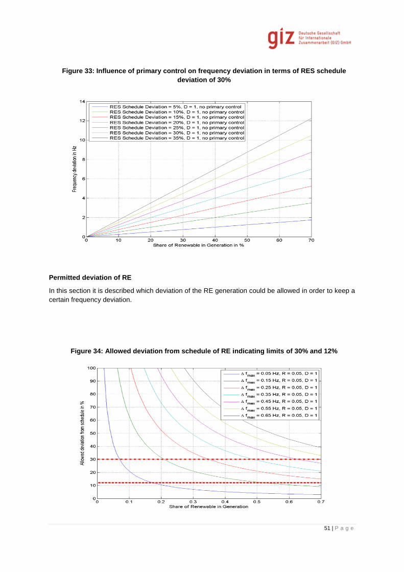
51 | P a g e
Figure 33: Influence of primary control on frequency deviation in terms of RES schedule
deviation of 30%
Permitted deviation of RE
In this section it is described which deviation of the RE generation could be allowed in order to keep a
certain frequency deviation.
Figure 34: Allowed deviation from schedule of RE indicating limits of 30% and 12%

52 | P a g e
Figure above shows the allowed deviation from schedule to keep certain frequency deviations
depending on the share of RE. With a limit of 30% deviation from schedule and a frequency deviation
up to 0.25 Hz a share of RE up to 35% would be possible. This is calculated for all generators
contributing to primary control. Figure below shows the influence of different droops regarding a
frequency deviation of 0.25 Hz.
Figure 35: Allowed deviation from schedule of RE indicating limits of 30% and 12% with
variable primary control provision.
The above simulation show that implementation and real use of primary control or FGMO as required
in the grid code would help to accommodate higher fluctuations or deviation from schedule. This is
shown for the share of renewables regarding the forecast uncertainty, but it is also true for all other
deviations caused by other incidents.
Primary control reserves are usually covering a time span of only several minutes and their task is to
contain the frequency within a given limit. Primary reserves should be set free as soon as possible to
be available again for coming control activities. Additionally, often the generation of primary reserve is
relatively costly.
From these considerations the three step approach is current best practice, where primary reserves
are replaced by secondary reserves and secondary reserves again by minute reserve. Primary
reserve is necessary for frequency control in grid operation. The functionalities of secondary control
and minute reserve are partly provided by the DSM (UI) approach, but it is highly decentralized and
driven by decision of individual businesses (generators). Thus the availability and activation of
sufficient secondary or minute reserve cannot be guaranteed.
We recommend the strict implementation of primary control functionalities in the power plants and to
involve also RE generators. Furthermore, a market or other incentive should be provided, where
secondary and minutes reserves can be provides with a secure availability.

53 | P a g e
4.3 Methodology of reserve dimensioning
There different reasons of imbalances in an interconnected system. The following types of imbalances
have to be considered:
Disturbance or full outage of a Power Generating Module, HVDC interconnector or load - this
type of imbalance is generally used for the calculation of the Reference Incident of a
Synchronous Area or a Dimensioning Incident of a LFC Block in Europe;
Continuous variation of load and generation – stochastic fast (noise) disturbance caused by
fast variations of consumption and generation;
Stochastic forecast errors – stochastic slow disturbances caused by forecast errors of load
(e.g. due to untypical weather) and RES generation;
Deterministic imbalances – a deterministic disturbance caused by the deviation between load
and step-shaped schedules which reaches its peak at the time point with the highest change
of schedules (mostly visible at the hour shift) and causes deterministic Frequency Deviations.
Network splitting - these imbalances are generally out of the dimensioning of the
Synchronous Area as they lead most likely to an emergency situation in a part or in all of the
Synchronous Area, nonetheless the disturbance is taken into account by formulation of
geographic constraints.
Figure 36: Simplified illustration of imbalance types (source: entso-e)
Dimensioning of Reserves in general has to take into account all of the corresponding effects and has
to respect
expected magnitude of the imbalance;
expected duration of the imbalance;
possible mutual dependency of imbalances; and

54 | P a g e
Imbalance gradients.
Methodologies for the dimensioning of reserves for frequency regulation are described in the following
sections.
4.3.1 Primary reserve
For the dimensioning of the primary reserve the entso-e methodology is described as best practice
approach. In Europe, there are different synchronous areas and depending on the overall system size
of these areas there are (n-1) or (n-2) approaches used. For bigger systems the probability of
consecutive failures or events is assumed with a higher probability. Thus for the Continental Europe
synchronous area (n-2) is considered and will be focused on here, because the whole India
synchronous system is seen as a highly complex system demanding strict security rules.
4.3.1.1 Dimensioning
The objective of the frequency containment process is to maintain a balance between generation and
consumption within the Synchronous Area and to stabilize the electrical system by means of the joint
action of respectively equipped FCR Providing units and groups. Appropriate activation of FCR results
consequently in stabilization of the system frequency at a stationary value after an imbalance in the
time frame of seconds.
The basic dimensioning criterion of the FCR is to withstand the reference incident in the synchronous
area by considering the maximum frequency deviation for the containment and the maximum steady-
state frequency deviation for the stabilization of the system. The steady-state frequency deviation was
also simulated for the assessment of the balancing needs before.
The reference incident has to take into account the maximum expected instantaneous power
deviation between generation and demand in the synchronous area and can be determined by taking
into account at least
the loss of the largest power plant;
loss of a line section;
loss of a bus bar;
the loss of the largest load at one connection point; as well as
a loss of a HVDC interconnector
That may cause the biggest active power imbalance with an N-1 failure. Significant fluctuations of
variable RES occur on a wider time frame and are not taken into account.
In larger systems like continental Europe or all-India with many units there is a larger probability of an
additional loss of generation, consumption or injection before the system has recovered from a
previous loss within the design window. A more detailed analysis has been performed for the
continental Europe system to estimate a reasonable size of reference incident to assure that incidents
leading to an even greater imbalance are extremely rare, but within some boundaries since the
different type of reserves must be procured according to the size of the reference incident with
consequences on the overall efficiency of the system.
When a unit trips, it is assumed that the FCR recover the balance of the system in the same minute
as the deployment time of FCR in the continental Europe system is 30 seconds. The loss of
generation is counteracted only with FCR so assuming that the system starts in perfect balance and
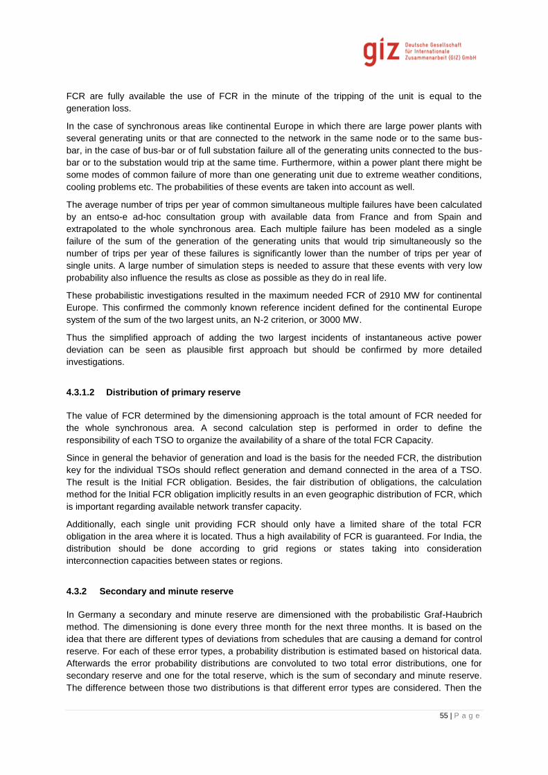
55 | P a g e
FCR are fully available the use of FCR in the minute of the tripping of the unit is equal to the
generation loss.
In the case of synchronous areas like continental Europe in which there are large power plants with
several generating units or that are connected to the network in the same node or to the same bus-
bar, in the case of bus-bar or of full substation failure all of the generating units connected to the bus-
bar or to the substation would trip at the same time. Furthermore, within a power plant there might be
some modes of common failure of more than one generating unit due to extreme weather conditions,
cooling problems etc. The probabilities of these events are taken into account as well.
The average number of trips per year of common simultaneous multiple failures have been calculated
by an entso-e ad-hoc consultation group with available data from France and from Spain and
extrapolated to the whole synchronous area. Each multiple failure has been modeled as a single
failure of the sum of the generation of the generating units that would trip simultaneously so the
number of trips per year of these failures is significantly lower than the number of trips per year of
single units. A large number of simulation steps is needed to assure that these events with very low
probability also influence the results as close as possible as they do in real life.
These probabilistic investigations resulted in the maximum needed FCR of 2910 MW for continental
Europe. This confirmed the commonly known reference incident defined for the continental Europe
system of the sum of the two largest units, an N-2 criterion, or 3000 MW.
Thus the simplified approach of adding the two largest incidents of instantaneous active power
deviation can be seen as plausible first approach but should be confirmed by more detailed
investigations.
4.3.1.2 Distribution of primary reserve
The value of FCR determined by the dimensioning approach is the total amount of FCR needed for
the whole synchronous area. A second calculation step is performed in order to define the
responsibility of each TSO to organize the availability of a share of the total FCR Capacity.
Since in general the behavior of generation and load is the basis for the needed FCR, the distribution
key for the individual TSOs should reflect generation and demand connected in the area of a TSO.
The result is the Initial FCR obligation. Besides, the fair distribution of obligations, the calculation
method for the Initial FCR obligation implicitly results in an even geographic distribution of FCR, which
is important regarding available network transfer capacity.
Additionally, each single unit providing FCR should only have a limited share of the total FCR
obligation in the area where it is located. Thus a high availability of FCR is guaranteed. For India, the
distribution should be done according to grid regions or states taking into consideration
interconnection capacities between states or regions.
4.3.2 Secondary and minute reserve
In Germany a secondary and minute reserve are dimensioned with the probabilistic Graf-Haubrich
method. The dimensioning is done every three month for the next three months. It is based on the
idea that there are different types of deviations from schedules that are causing a demand for control
reserve. For each of these error types, a probability distribution is estimated based on historical data.
Afterwards the error probability distributions are convoluted to two total error distributions, one for
secondary reserve and one for the total reserve, which is the sum of secondary and minute reserve.
The difference between those two distributions is that different error types are considered. Then the

56 | P a g e
fixed targets for the deficit probability are applied to both distributions to calculate the needed
reserves. In the following figure the principle of the method is illustrated:
Figure 37: Schematic representation of the Graf-Haubrich method
The minute reserve is the difference between the total reserve demand and the secondary reserve
(CONSENTEC 2008). The following table shows the considered error types and their attribution to the
different reserve types.
Table 9: Error types considered in the Graf-Haubrich method (CONSENTEC 2010)
Error type Determination Secondary
reserve
Total
reserve
Load noise Empirically determined distribution based
on time series of vertical net load X X
Forecast errors Empirically determined distribution based
on actual reserve activations corrected for
power plant outages
X
Schedule steps Stochastic ramping model for the sum of
schedule steps with foreign TSOs X X
Power plant
outages
Stochastic distribution based on convolution
of historic outages of all power plants > 100
MW
X X
Hour steps Empirically determined distribution of the
difference between 15-min. and 1-h mean
value of the forecast error
X
Today in Germany the following deficit probabilities are used. (A total deficit probability of 0.05 %
means that in about 4.4 hours per year the secondary and minute reserves are not sufficient.)
Table 10: Parameterization of the Graf-Haubrich method (CONSENTEC 2010)
Total deficit probability 0.05 % ~ 4.38 h/a
Deficit probability due to insufficient total reserve 0.045 % ~ 3.94 h/a
Deficit probability due to insufficient secondary reserve 0.005 % ~ 0.44 h/a
In the following figures the procured amounts of secondary control and minutes reserves of the last
years are shown.
* * * *Posit ive
Reserves
Negat ive
Reserves
=Power plant
outages
Load
noise
Forecast
errors
Schedule
steps
Hour
steps

57 | P a g e
Figure 38: Procured secondary reserve capacity in Germany for each quarter of the year
Figure 39: Procured minute reserve capacity in Germany for each quarter of the year
At the moment also dynamic dimensioning methods are discussed which make use of shorter
dimensioning horizons like one day. These methods are able to consider forecasts for wind power, PV
power, load, temperature, etc. to fit the reserves better to the specific situation in each hour of the
day. This leads to more reserves in critical situations and less reserve in the rest of the time and so to
a higher security level with less reserve in average. One example is presented in (Jost et al. 2015).
2012 2013 2014 2015-2500
-2000
-1500
-1000
-500
0
500
1000
1500
2000
2500
year
MW
Procured secondary control reserves in Germany for each quarter
2012 2013 2014 2015-3000
-2000
-1000
0
1000
2000
3000
year
MW
Procured minute reserves in Germany for each quarter
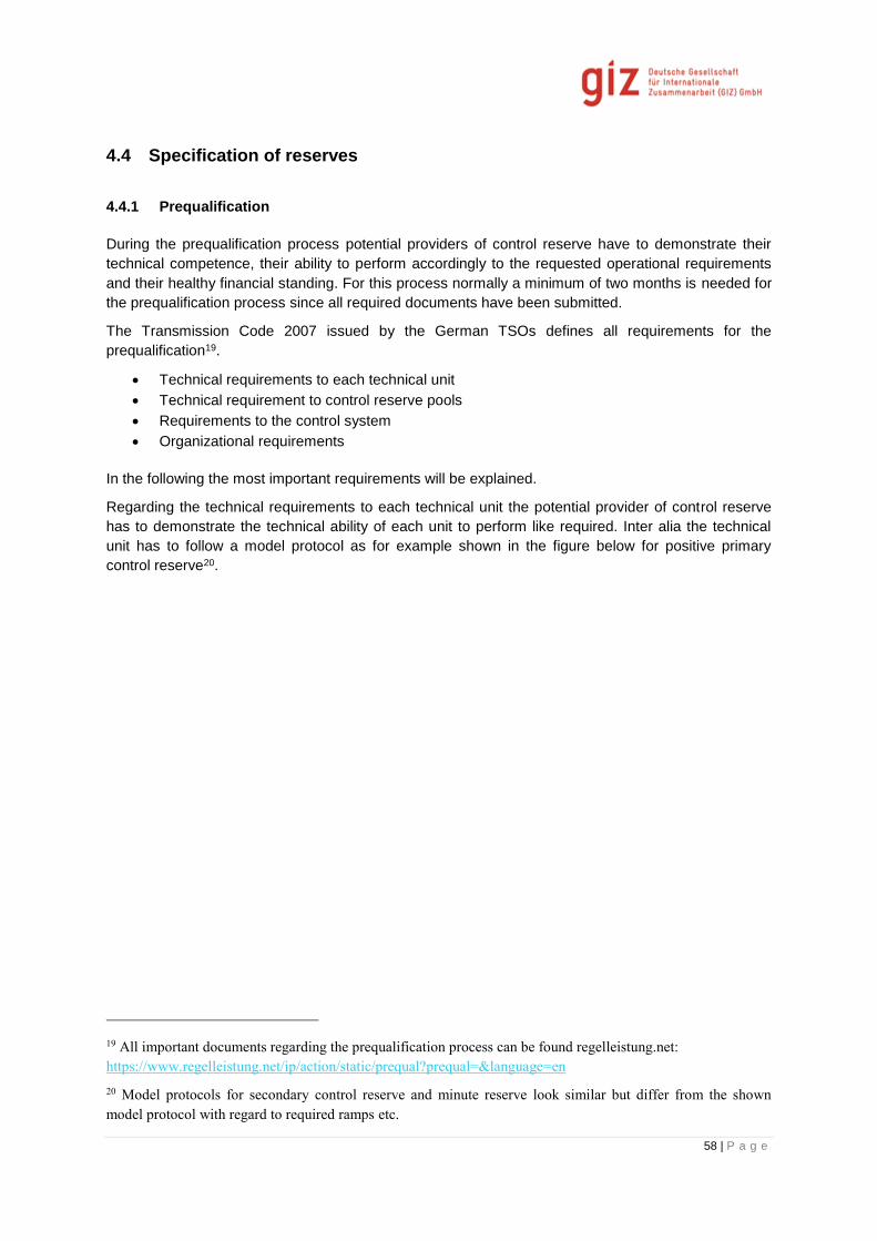
58 | P a g e
4.4 Specification of reserves
4.4.1 Prequalification
During the prequalification process potential providers of control reserve have to demonstrate their
technical competence, their ability to perform accordingly to the requested operational requirements
and their healthy financial standing. For this process normally a minimum of two months is needed for
the prequalification process since all required documents have been submitted.
The Transmission Code 2007 issued by the German TSOs defines all requirements for the
prequalification19.
Technical requirements to each technical unit
Technical requirement to control reserve pools
Requirements to the control system
Organizational requirements
In the following the most important requirements will be explained.
Regarding the technical requirements to each technical unit the potential provider of control reserve
has to demonstrate the technical ability of each unit to perform like required. Inter alia the technical
unit has to follow a model protocol as for example shown in the figure below for positive primary
control reserve20.
19 All important documents regarding the prequalification process can be found regelleistung.net:
https://www.regelleistung.net/ip/action/static/prequal?prequal=&language=en
20 Model protocols for secondary control reserve and minute reserve look similar but differ from the shown
model protocol with regard to required ramps etc.

59 | P a g e
Figure 40: Model protocol for the prequalification of a technical unit for positive primary
control
Thermal units providing secondary control reserve always have to be synchronous to the grid
whereas hydraulic units also can be in standstill if they are able to reach the amount of prequalified
control reserve within five minutes.
All three types of control reserve can be provided not only by a single unit but also by pools of several
units. Pooling for all three types of control reserves is allowed within one control area. Pools of units
that are located in different control areas are only allowed for secondary control and minute reserve to
reach the minimum product size. Furthermore the provider has to provide additional units for the
replacement of failed units as he has to guarantee the availability of the complete offered control
reserve over the whole product length. If the provider is not able to fulfill this requirement the TSO is
allowed to delete the payments for not provided capacity respectively energy. Additionally the provider
has to pay additional costs of appropriate substitution. In the case of repeated breaches of contract
within one year the TSO can charge the provider a contractual penalty and in the worst case the
prequalification can be withdrawn (www.regelleistung.net 2011, 2012, 2013).
Providers of primary control reserve and minute reserve only have to inform the TSO online about
each unit’s current feed-in or draw-off and some additional information. Providers of secondary control
reserve, however, have to meet much more demanding requirements, e.g. a redundant design of all
communication channels, a control cycle of maximum four seconds, etc.
The most important organizational requirement is the constant availability of a contact person for the
TSO during the provision of control reserves.
4.4.2 Product specifications
All tenders and their anonymized results are published on www.regelleistung.net. The tendered
amount of primary control reserve is determined by the ENTSO-E and changes every year whereas
the amounts of secondary and tertiary control are calculated by the German TSOs every quarter of
the year. The control reserve market is organized as a pay-as-bid market. For primary control
reserves the product length is one week (Monday to Sunday). The offering time is normally 10:00 on

60 | P a g e
the Tuesday before. The tenders for primary control reserves are ‘symmetrical’, that means that there
are no separate tenders for positive or negative reserve. The minimum lot size is +/- 1 MW with
increments of 1 MW. There is only a capacity price and no energy price.
The product length for secondary control reserve is also one week like for primary control reserve. But
the products are divided in peak (Monday to Friday from 8:00 till 20:00) and off-peak (Monday to
Friday from 0:00 till 8:00 and from 20:00 till 24:00 and on Saturday and Sunday as well as on national
holidays) and there are separate tenders for positive and negative secondary control reserve. The
offering time is usually 10:00 on the Wednesday before the delivery week. The minimum lot size is 5
MW with increments of 1 MW. Offers are accepted from the merit order list which is based on the
offered capacity price. The call for the delivery of secondary control reserves follows the order of the
offered energy prices from low to high prices. The energy price is paid for actually delivered energy on
top of the capacity price.
For minute reserve a product length of 4 hours applies (6 time slices per day). The offering time is
always at 10:00 for the next day and for the following weekend and/or holidays. Apart from that the
same conditions as for secondary control apply. Providers of all three types of control reserve have to
be able to deliver balancing power equal to the offered capacity over the whole product length.
Table 11: Reserve product specifications
Primary control
reserve
Secondary control reserve Tertiary control
reserve
Auction time Weekly
(on Tuesdays for
the next week)
Weekly
(On Wednesdays for the next week)
Daily
(10:00 for next
day and
following
weekend or
holidays)
Product time
period
One calendar
week
Peak (Monday to Friday from 8:00 till
20:00) or off-peak(Monday to Friday from
0:00 till 8:00 and 20:00 till 24:00 as well
as weekends and national holidays from
0:00 till 24:00) of one calendar week
4 h (6 time slices
per day)
Product type Positive and
negative reserve
in one product
Positive and negative reserve separated Positive and
negative reserve
separated
Product size ≥ 1 MW
symmetrical
positive and
negative reserve
≥ 5 MW ≥ 5 MW
Product
increment
1 MW 1 MW 1 MW
Compensation Capacity price Capacity and energy price Capacity and
energy price

61 | P a g e
4.4.3 Recommendation for the introduction of restoration reserve as ancillary service
The current CERC draft on the introduction of ancillary services focuses mainly on frequency
regulation and minute reserve, which has the functionality of reserve replacement in a three step
reserve scheme.
The market development for reserves is influenced by effects from the demand and the supply side.
Important factors and their expected effect on the market efficiency in Germany are summarized in
the following table.
Table 12 - Factors influencing demand and supply of the control reserve market in Germany
Influence on demand Tendency Influence on supply Tendency
Extension of control zones reducing Reducing duration for offered
services, allowing pooling of units,
reducing minimal offered power
increasing
Increased balancing
activities using intra-day
markets
reducing Allowing new providers, e.g.
decentralized generators
(including power-to-heat or
backup generators)
increasing
Growing installed capacity
of renewables, absolute
effect of forecast failure
rises
increasing More power plants operating in
partial load, reducing minimal load
of power plants
increasing
Optimizing of feed-in
forecast of renewables
reducing Increased grid/ line contingencies
and lagged grid extension on
transmission level
reducing
Source: [Dena 2013]
Following the influencing factors stated in the table above recommendations can be derived for the
introduction of RR as ancillary service in India:
Create a liquid market and push technical innovations by extension of the eligibility
criteria.
o The eligibility should be defined technology and provider neutral, i.e. only the
capacity to provide (positive or negative) reserve of a specified power and
duration should be asked.
o Reserve products should be addressed as positive and negative reserve
separately. This increases implicitly the types of units that can participate in the
market. For instance, in a negative reserve market also plants running on full load
can participate or demand response of industrial customers can be stimulated. In
a positive reserve market also stand-by generators like industrial backup systems
could be involved.
Foster flexibility with short-term and near-time products.
o Allow for near-time balancing activities through intraday markets and late gate-
closure in bidding processes.
o Keep the duration of the period short in which reserve has to be allocated for a
bid.
Involve decentralized resources by allowing to pool smaller units.

62 | P a g e
o Especially to deal with the involvement of a higher number of potentially smaller
units a pre-qualification procedure will be necessary. Such a procedure should
comprise requirements for power delivery as well as for communication between
the despatcher and the provider.
During a pre-qualification also local grid conditions should be taken into account. Maybe pooling can
be restricted to specific grid areas or regions.
4.4.4 Implementation of grid control cooperation
Whereas all LFC Blocks provide mutual support by the supply of primary control power during the
primary control process, only the LFC Block affected by a power unbalance is required to undertake
secondary control action for its correction. Consequently, only the controller of the LFC Block in which
the imbalance between generation and consumption has occurred will activate the corresponding
secondary control power within its LFC Block. Parameters for the secondary controllers of all LFC
Areas need to be set such that, ideally, only the controller in the zone affected by the disturbance
concerned will respond and initiate the deployment of the requisite secondary control power.
Following the principal to activate positive or negative FRR in the control area where the deviation
occurs, antagonistic activation in neighboring control areas is possible. And not only possible, but
happens regularly showing potential for optimization. This led to the implementation of regional
cooperation of power balancing in central Europe, the so-called International Grid Control
Cooperation (IGCC). Starting in 2006 with the four control areas in Germany, today also Denmark,
The Netherlands, Czech Republic, Belgium, Austria and Switzerland are involved in ‘Imbalance
netting’.
The market process of is more complex, because cross border transfer capacities have to be taken
into account. Despite this complexity the imbalance netting shows good results both in terms of
energy efficiency and in terms of costs for reserve provision.
The principal organization and economic results are shown in the following figures (source: entso-e):

63 | P a g e
Figure 41: Technical implementation of Imbalance Netting in IGCC
Figure 42: Example of pro-rata distribution of netting potential with congestion
correction

64 | P a g e
Figure 43: Value of netted imbalances per country
Imbalance netting is possible in interconnected and neighboring areas (states, regions or countries).
Transfer capacities have to be taken into account. But the results are showing that is recommended
to cooperate between control areas in order to avoid antagonistic control in neighboring areas.
4.5 Voltage control
System voltage is another key performance metric of the power system. Voltage is a local measure,
which differs in every power system node, both on transmission and distribution level. Voltage is
influenced by reactive power. Reactive power transmission causes losses, and as reactive power can
be more easily generated at the site where it is needed, in general reactive power transmission is
tried to be avoided.
The voltage levels of the power system nodes constitute the voltage profile of the power system. The
voltage profile must be maintained within prescribed ranges at every node on the power system to
maintain power quality, avoid damages to components (either networks’ or customers’) in case of
excessively high voltage and prevent malfunctions in case of excessively low voltage, as well as
maintain power system voltage stability.
This is achieved by a combination of three tools:
Preventing unnecessary transits of reactive power (mainly through requirements for
customers and pricing of reactive power transits);
Adding new network assets to support the active and reactive transits;
Balancing (dynamically) the generation and consumption of reactive power (i.e. capacitive
and inductive reactive power) in the voltage controlled nodes of the system.
65 | P a g e
Control of voltage is tightly connected to reactive power control. Voltage can be controlled through
voltage control, reactive power control, power factor control or by a combination of two of these, so
they are often referred to as voltage/reactive power control.
As regards TSOs real time operations and operational planning, Voltage control has two targets:
Voltage profile management and reactive power dispatch (steady state): The aim is to keep
the voltage profile close to the desired profile and within the tolerance band margins with time
frame of hours. This entails minimization of the system active power losses while keeping
steady-state system security in the face of possible contingencies.
Maintaining voltage stability (dynamic): This service controls the network voltages in a
dynamic time frame (seconds to minutes). The aim is to prevent a slow voltage collapse event
or limit its depth and extension in case of an incident (loss of main, loss of generation unit).
4.5.1 Market design for voltage support
In view of appropriate market designs for reactive power procurement, the following differences
between active and reactive power were highlighted as outcome of the European research project RE
services:
Reactive power should be supplied close to the point of demand. Otherwise the effect is
limited and on the way to the point of demand, reactive power congests the power lines
limiting the capacity to transport active power. In particular the possibilities to provide reactive
power from lower voltage level to higher voltage levels are limited;
The demand for reactive power is relatively low compared to the demand for active power in a
power system. Some generators can offer reactive power at very low cost.
These factors limit the number of possible offers for reactive power demand. Also, the costs of
implementing trading platforms of standard reactive power products and the trading transaction costs
might not be justified by the traded volume.
On the other hand, the need for reactive power and the need to diversify reactive power sources grow
with the increased penetration of renewables, as the market share of conventional power plants
(which traditionally delivered reactive power) steadily decreases. Thus, reactive power is often either
required as a mandatory service by the TSO or is tendered longer term by the TSO, typically on an
annual basis.
4.5.2 Examples of current approaches to contract voltage support in Europe
Examples of more detailed technical specifications and practices for the voltage control services from
different countries were collected during the RE services project and are presented in the following:
In Denmark, Germany and Spain, the provision of the reactive power for voltage control services by
conventional generators is mandatory. Generators which provide reactive power in Germany and
Denmark, do so via bilateral agreements with their respective TSOs. In Germany, wind generators
(connected after January 2009) get a bonus for delivering reactive power, while this is not true for PV
generators. In Denmark this service is not remunerated and for wind power, it became a requirement
in the grid code of 2010. In Spain, special regime generators not involved in the active power market
are allowed to trade on a tendering market for the provision of reactive power services. Over and
above the basic remuneration there is bonus/penalty system based on producing within a particular
power factor range depending on the load situation (Twenties, 2012).

66 | P a g e
Spain: voltage control mandatory for all conventional generation and non-remunerated. In case of
RES there is a power factor set-point of 1 that would imply receiving a bonus or a penalization if this
power factor is not maintained. TSO (REE) is able to send power factor set-points different than 1 to
generators larger or equal to 10 MW. If this set-point is maintained, the generator will receive a bonus
and if it is not maintained, it will be penalized. There is a proposal in the process of approval for
allowing generators to have voltage control in a similar scheme to the conventional generation, but
with bonuses and penalizations.
Portugal, on the DSO network, has capacitor banks installed on HV/MV substations for grid loss
compensation and voltage control. It has been recently imposed that most of Distributed Generation
on the DSO network must have the possibility of injecting reactive power.
Great Britain: NGC procures reactive power through both market-based tender processes and the
default arrangements for all generators rated at over 100 MW and default arrangements procure
reactive power accordingly. The default arrangements remunerate generators for reactive power
according to utilization on a €/MVArh basis (Mutale and Strbac 2005).
Ireland: Eirgrid: Steady state reactive power is shaped as a product of Reactive Power Capability. It
is defined as the reactive power range (in MVAr) that can be provided across the full range of active
power output. Payment for Reactive Power Capability will be based on a rate that is scaled by the
ratio of the active power output range (Maximum Generation – Minimum Generation) to the
Registered Capacity of the generator. It is proposed that payment is based on the reactive capability,
irrespective of the dispatched output of the generator. Synchronous and non-synchronous sources as
well as synchronous compensators are eligible for this product. This restructured product definition is
illustrated in Figure 18 for a hypothetical 100 MW generator. Payment will be based on a rate that is
scaled by the ratio of the active power output range (Maximum Generation – Minimum Generation) to
the Registered Capacity of the generator. The difference is shown between what the plant can offer
(red) and what TSO can use (blue). (Eirgrid and SONI, 2012a)
In France, three sources of reactive power management are manageable by Network Operators.
Large generators connected to TSOs network are required to provide reactive power management
capability, either absorption or injection according to their situation on the network. They can be used
as synchronous compensators. Taking into account their proper constraints of stability the set points
of operation are directly managed by the TSOs. The TSOs operate compensation devices and in
some cases reactors on its own network and compensation devices are connected on the MV bus
bars of primary substation. They are operated by DSO within an agreement with the TSO. Only the
first one is considered an AS and is subject payment. Actual delivery of service is periodically
checked.
Another detailed description of the reactive power market of California is given in the annex. Also for
this case study the conclusion is, that due to its locational effect and use, reactive power and voltage
support is a reliability service that cannot be procured through a market via a competitive auction as
other ancillary services because of market power concerns. Voltage support is mainly procured
through long-term contracts with reliable must run units.
4.5.3 Voltage support by RES
Voltage support induces costs for VAR-RES but can, in some cases, help system operators to
manage their network in the most efficient way. In areas with only a small amount of VAR-RES plants
providing the service needed by the network operator, a non-remunerated mandatory band
requirement as part of the grid code could be complemented with payment for additional support to
grid operation, provided such costs are recognized by the regulator and recoverable by the system
operator. If the number of service providers is large enough to create a competitive market, voltage
67 | P a g e
support could be reimbursed in a competitive process, either in a regular bidding process or an
auctioning arrangement, irrespective of whether the contracting is for short time horizons i.e. from
days to weeks, or for longer time horizons up to several years;
If a tendering or auctioning process is applied, it should involve:
An analysis of the need for reactive power carried out by the relevant network operator
(TSO/DSO) and a forecast for future locational needs;
Based on such an investigation, a tender for reactive power within a certain perimeter should
be published or an auctioning system should be put in place to receive the lowest cost
reactive power provision;
The best offer (or best offers) is awarded with a fixed reimbursement for the reactive power
provided to the system and a minimum off-take guarantee to ensure investment security.
4.6 Black start
Back start services refer the combined set of those services that are required to restore the grid after
a partial or complete blackout. These services are required to provide the following:
Initial energizing power for starting big conventional plants.
Communication and control infrastructure to coordinate a restart of all scheduled generators
Establish islands as a first step and resynchronize the complete grid
Black start services are critical; however in a well-managed grid they are seldom required.
Additionally, the capability of house-load operation of power plants is supporting network restoration
processes.
Regarding the market design for black start services similar considerations as for voltage support
apply. House load operation should be mandatory for power plants of a significant size (e.g. above
200 MW). Additional black start capabilities can be requested by the system operator for specified
grid areas. Usually only a limited number of bidders could be involved and a tendering process can be
used to introduce a competitive market.
4.7 RES capabilities to provide ancillary services
The European research project RE services (www.reservices-project.eu) made a thorough
assessment of the capabilities and market opportunities of wind and PV power regarding ancillary
services. Main outcomes are given below:
RE services found that the technical capabilities of wind and solar PV for the provision of GSS
depend on the plant size and the extent of their output aggregation19. These two aspects were used
as criteria for rating the degree of deployment of technical features enabling the provision of grid
support services (GSS) by both technologies.
Also, technical capabilities were evaluated against industry standards, prequalification procedures,
connection and operational requirements contained in grid codes20 and the so-called European
Network Codes. However, RE services found that these documents may not always contain technical
requirements for GSS or may be inadequately defined.
The assessment of technical capabilities is shown in the two tables below. The criteria and rating
scale used is shown below the first table. The table also contains numerical references to further
details described in the second table.

68 | P a g e
Table 13: Wind and Solar PV Technology Capabilities for Gas Provision
Systematic investigation of wind power and solar PV technology, confirms that they are technically
capable to provide grid support services for frequency, voltage and system restoration assuming an
adequate procedural and economic framework is present. The technical operational functions
required are either state of the art capabilities of the existing hardware or measures that can be
implemented at a reasonable cost. The feasibility of providing services by enhanced plant capabilities
is confirmed by TSOs, for example in Spain where voltage control by wind power plants on the
specific transmission nodes leads to a significant improvement with fast response. The German/
Spanish case studies within RE services demonstrate that letting the DSO use GSS from VAR-RES
generation connected to its own system contributes to cost-efficient voltage management.
Participation of VAR-RES in system restoration has not been considered until now. Certain required
functionalities are available but their implementation in specific restoration strategies needs further
investigation.

69 | P a g e
Implementing enhanced capabilities will involve additional investment, and the deployment of the ser-
vices will also involve costs. For both wind and solar PV the additional CAPEX costs involved for
enhanced provision are relatively low and — provided appropriate cost recovery/market mechanisms
are in place — their deployment should be commercially feasible. Only for small PV systems the
impact of required communication components will result in high additional CAPEX costs. In general,
both for wind and PV, OPEX costs — notably upward readiness costs — represent the highest costs
required to make frequency services available.

70 | P a g e
Table 14: Explanations and References for Wind and Solar Technology Capabilities

71 | P a g e
4.8 German Scenario
Short term balancing is done by generation or consumption units which increase or decrease their
generation respectively their consumption depending on the frequency or on request of the TSO.
These procured capacities are called control reserves. The German TSOs procure three different
types of control reserves:
4.8.1 Primary control reserve
Primary control reserve is used for the fast stabilization of the grid frequency after a disturbance in the
time frame of seconds. It is activated simultaneously by all contracted providers in the UCTE
synchronous area, irrespective whether the imbalance was caused within the TSO’s control area or
not. It is not activated by a central sent signal but individually depending on the measured grid
frequency. The complete activation of the reserve has to be done within 30 seconds with a linear
ramp. In the UCTE synchronous area 3000 MW of primary control reserves are procured. This
capacity is split up between all TSOs according to their annual peak load. The German TSOs for
example had to procure 578 MW in 2015. The German TSOs spent 82.27 Mio. EUR in 2012 for the
procurement of primary control reserve (Bundesnetzagentur 2014b).
There is no central activation for PCR, rather the existing technical units provide PCR according to the
network frequency locally metered. TSOs are allowed to require – as proof of provision – the actual
values which the participating technical units fed in over time.
4.8.2 Secondary control reserve
Secondary control is used to balance the energy within each TSO’s control area, should bring the grid
frequency back to its nominal value and replace primary control. It has to be completely activated
within five minutes and the activation is immediately done by the TSO. For the procurement of
secondary control reserve capacity, 267.07 Million EUR were spent in 2012 (Bundesnetzagentur
2014b).
Secondary control reserve is automatically activated by the power-frequency controller which
considers deviations of power exchange as well as frequency from the corresponding set points.
According to the merit order for activated control energy bids are activated, with the German grid
control cooperation guaranteeing an all-German merit order independently from power plants
connected to the controller.
This selection helps to minimize the costs of deployment related to the required control energy of
each type of control reserve. In order to verify the effective provision, TSOs are entitled to request
various information, e.g. on actual values of feed-in and on the provided secondary control reserves
by the participating technical units over time. The bidders have to provide them online.
4.8.3 Tertiary control reserve
Tertiary control partially complements secondary control and finally replaces it. Minute reserve’s or
tertiary control reserve’s activation has to be completed within fifteen minutes. The activation is done
electronically since 2012, whereas the decision if minute reserve should be activated is made
manually. In 2012 the German TSOs spent 67.42 Mio. EUR on the procurement of minute reserve
capacity (Bundesnetzagentur 2014b).
72 | P a g e
Additionally immediately and quickly interruptible loads are procured by the TSOs since the end of
2012. In this context interruptible loads are large consumption units which consume a large volume of
electricity in a more or less continuously way and can reduce or interrupt their consumption on short
notice for a certain time span. Usually control reserves are provided by large thermal and hydro power
plants, pumped hydro storages and loads. Recently also smaller biomass power plants gained in
importance.
Minute reserves are activated by the TSO in case of foreseeable longer lasting failures of system
balance to replace the more valuable secondary control reserve.
4.8.4 Grid control cooperation
In general, the required reserves are procured in each TSO’s own control area. However, since 2010
the German TSOs cooperate within a Grid Control Cooperation (Netzreglerverbund). This means that
their four control areas are operated as one control area. The functionality of this Grid Control
Cooperation is assured by four modules (www.regelleistung.net):
1. Prevent counteracting control reserve activation
2. Common dimensioning of control reserve
3. Common procurement of secondary control reserve
4. Cost-optimized activation of control reserve
As a consequence of the Grid Control Cooperation there are no restrictions for the procurement and
activation of control reserves in Germany.
The Grid Control Cooperation should be extended to neighboring countries. Until now Denmark, the
Netherlands, Switzerland, the Czech Republic, Belgium and Austria have joined the first module
(www.regelleistung.net).
Additionally Switzerland, Austria and the Netherlands procure a part of their required primary control
reserves (71 MW, 67 MW respectively 67 MW) via a common auction with the German TSOs. This
auction is open for all prequalified providers of primary control reserve from these three countries.
The Agency for the Cooperation of Energy Regulators (ACER) aims at an integrated electricity
balancing market for whole Europe to improve the efficiency of frequency control. To eliminate the
existing barriers (different balancing products, different pricing, etc.), ACER adopted its Framework
Guidelines on Electricity Balancing in 2012. Core elements of the Framework Guidelines are models
for cross-border exchanges of balancing energy that should result in one European platform for the
procurement of control reserves. Additionally the harmonization of key elements such as balancing
products, balancing energy prices, etc. is pushed to pave the way to a fully integrated electricity
balancing market (ACER 2014). Based on these Framework Guidelines ENTSO-E has improved the
Network Code on Electricity Balancing (ENTSO-E 2014).
The procurement of control reserves is done via tenders on the common internet platform of the four
German TSOs www.regelleistung.net. To offer control reserve potential providers have to complete a
prequalification procedure which is described in the following chapter and sign a framework contract.
A list of all prequalified providers for each type of control reserve can also be found on this platform21.
21 https://www.regelleistung.net/ip/action/static/provider

73 | P a g e
Table 15: Requirements of the different types of control reserves
Primary control
reserve
Secondary control reserve Tertiary control
reserve
Purpose Stabilize grid
frequency after
a disturbance
Balance control areas, bring
grid frequency back to
nominal value, replace
primary control
Complement and
replace secondary
control
Time until complete
activation
30 sec 5 min 15 min
Reaction time immediately 5 min, 30 sec until first
change of power for pooled
reserve providers22
15 min
Activation Local, static
relation to the
frequency
Immediately by the TSO via
set points
Automatically by
Merit Order List
Server (MOLS)
Number of
prequalified providers
(July 2014)
20 27 38
4.9 Status of ancillary services in India
4.9.1 Definition and Scope
The CERC Power Market Regulations 2010 has made provisions for introduction of the Ancillary
Services in the Indian Electricity Market in the future. Regulation 4(viii) defines Ancillary Services as
follows:
“Ancillary Services Contracts – These contracts are for ancillary services. Ancillary Services in power
system (or grid) operation are support services necessary to support the power system (or grid)
operation for maintaining power quality, reliability and security of the grid, e.g. active power support
for load following, reactive power support, black start etc.” The CERC classifies ancillary services as
below.
Frequency Control ancillary services (FCAS)
These services are required to manage the imbalance between load and generation.
Frequency control services are further categorized into primary, secondary and tertiary
services based on their response time and duration of activations as explained in later
sections.
Network control ancillary services (NCAS)
NCAS are categorized into two main services. The first is reactive power and voltage control.
The second being network control. These services are explained in detail in later sections.
Black start
22 Pools providing secondary control reserve have to show a first reaction to the secondary control activation signal of the TSO
within 30 seconds, at the latest.

74 | P a g e
This service is required for re-energizing the complete grid or a section of the grid that has
lost all power due to major faults. It requires service providers (generators) to have the
capability to start generating without drawing startup power from the grid.
CERC has introduced the “Central Electricity Regulatory Commission (Ancillary Services Operations)
Regulations, 2015”. The objective of these regulations is to restore the frequency level at desired level
and to relieve the congestion in the transmission network.
These regulations shall be applicable to Reserves Regulation Ancillary Services Provider and
Regional Entities involved in the transactions facilitated through short-term open access or medium-
term open access or long-term access in inter-State transmission of electricity.
RRAS Provider means the inter-State Generating Stations (ISGSs) having un-requisitioned surplus
and eligible to participate in the RRAS.
Regulation down Service means an AS that provides capacity that can respond to signals or
instruction of the Nodal Agency for decrease in generation, within the technical limit and time limit, to
respond to changes in system frequency or congestion in the system.
Regulation up Service means an AS that provides capacity that can respond to signals or instruction
of the Nodal Agency for increase in generation, within the technical limit and within the time limit to
respond to changes in system frequency or congestion in the system.
4.9.2 CERC Draft Regulation on Ancillary Services Operation, May 2015
This draft focuses mainly on frequency regulation and minute reserve, which has the functionality of
reserve replacement in a three step reserve scheme. Comments to the draft were provided and
recommendations given in the report of task 2.2 “Report on instruments and measures to foster
variable Renewable Energy Sources (RES) in Germany and Europe”.
4.9.3 Petition on the inadequate response of FGMO, February 2015
The National Load Dispatch Center (NLDC) filed a petition on the inadequate response of the
inadequate response of the turbine governor to be used in power plants as Free Governor Mode
Operation (FGMO). FGMO is related to the implementation of primary frequency control. According to
the investigations and measurements performed by POSOCO the FGMO is by far not implemented
as required by the Indian grid code.

75 | P a g e
5 Market Options
5.1 Market Models
Two main models exist for structuring competitive wholesale generation markets - centralized
generation pools, either voluntary or compulsory; and systems based on bilateral contracts between
generators and buyers. The two models bring different approaches and requirements related to price
discovery, scheduling and dispatch and the role of the system operator. The following figures illustrate
these two models.
Figure 44 - Market Options
Source: KEMA Consulting
The two models are often used within a single system for different purposes. For example, the UK
BETTA system employs bilateral forward and spot markets as well as a voluntary net pool for
balancing.
Electricity Pools
An electricity pool is a centralized market facilitated by a market operator in which generators
compete with each other to supply power. The market operator sets the price through a process of
competitive bidding from generators to fulfil anticipated demand. Generators are required to submit
bids indicating the quantity of electricity they can generate at a given price. The market operator then
accepts bids from generators, starting with the cheapest, until the demand forecasts are met.
Successful bids are considered “in merit” while unsuccessful bids are left un-dispatched. Under most
systems, all successful bids will then receive the same price, based on the marginal bid received, or
some derivative of multipliers (e.g., Australia) or separate up/down prices (e.g., Finland balancing).
Pools usually operate on an hourly basis with generators competing to meet demand each hour. This
means there will be 24 different pool markets — and market prices — in a day.
Generators frequently hedge against price volatility in pool market with financial contracts for
difference (CfDs). In CfDs, two parties agree on a volume of electricity and a price. If the pool price is
higher than the agreed-on strike price, the CfD seller pays the buyer the difference; if it is lower, the
CfD buyer pays the seller the difference. If a generator produces the amount of electricity covered by
its CfD, then its revenues are fixed by the strike price. In CfDs, no physical delivery of electricity

76 | P a g e
occurs. In the case of the UK England and Wales pool, 90% of the electricity sold by the major
generators is covered by these contracts. Only 10% of electricity is actually sold at pool prices.
The following figure summarises the types of electricity pools option available.
Figure 45 - Types of electricity pool options
Bilateral Trading
Bilateral trading is a decentralized model in which generators and buyers enter into bilateral contracts
for sale of electricity. A producer can buy or sell in a bilateral trading arrangement. Contracts specify
the amount and the price of the electricity to be traded and when the trade will take place. At a set
time before delivery (gate closure), participants disclose their net contract sales and purchases to the
system operator. Each generator decides on when to dispatch, and the system operator is required to
manage any imbalances that occur.
Disparity between market participants’ notified contractual positions, and their physical delivered or
taken electricity indicates the level of imbalance on the system. The system operator has two options
for setting an imbalance pricing mechanism - a market price (e.g., Norway) or a punitive price (e.g.,
UK NETA).
Nearly all bilateral markets incorporate a balancing mechanism (BM) to facilitate system balancing.
This most often takes the form of a net pool (e.g., Belgium, France, Great Britain or the Netherlands)
in which producers must offer their entire available generation capacities for balancing purposes at
the time of final gate closure.

77 | P a g e
The following illustration provides a comparison between gross pool, net pool and bilateral trading
arrangements.
Table 16 - Comparison of Market Options
Gross pool Net pool Bilateral
Price
determination
• Determined by the market
operator based on demand
forecast (one-sided pool);
potential for a one and a
half-sided pool — with some
demand handled separately
• Usually unit-based offers (i.e.,
based on output of individual
generating assets)
• Determined by the market
operator based on forecasted
demand (one-sided pool)
or based on the quantity
demanded by buyers
(two-sided pool)
• Can be unit based or portfolio
based (i.e., based on total
owned generation)
• Energy treated as a
commodity
• Individual contracts
• Portfolio-based offers
Market
operation
• Centralized dispatch by
merit order
• Pricing of imbalances,
congestion management and
ancillary services integrated
into the
spot market
• Requires a detailed technical
knowledge of the authorized
generating units
• Centralized dispatch by merit
order post contractual
arrangements
• Requires a detailed technical
knowledge of the authorized
generating units
• Decentralized model that
relies on self-dispatch
• The system operator must
have the necessary
information and
infrastructure to ensure
system stability
• Constrained by contractual
arrangements, requires BM
• Separate markets for
imbalance pricing,
congestion management and
ancillary services
5.2 Pricing Models
Pricing models seek to provide fair return to generators, realize lowest possible price for consumers,
achieve liquid market, ensure security of supply and promote long-term investment. Pricing must also
suit different market types and transactions — forward markets vs. spot markets and bilateral
transactions vs. power exchanges. Pricing models fall into two categories — market based and cost
based.
Market-based pricing
It is a competition-based pricing mechanism for establishing a price for wholesale electricity based
upon the existing market conditions. The price is set by an agreement between the buyer and the
seller.
“Market-based” does not necessarily mean free market as market operators typically have the ability
to intervene when there are system security concerns. Market-based pricing models in generation can
be generally classified into the following types:
Pay-as-bid: Classic free-market pricing where sellers and buyers bilaterally agree on quantity
and price, often with the facilitation of intermediaries. This model almost inevitably requires a
balancing market, based on a central auction or similar mechanism, to ensure demand and
supply remain in continuous balance.
Bid-based auction: Generators issue bids to the market operator to provide a quantum of
electricity at a given time and price, which then determines a system marginal price based on
demand and supply conditions.

78 | P a g e
Locational marginal pricing (LMP): A more elaborate version of a bid-based auction that
takes congestion costs into account and creates many location-specific prices.
These pricing models may coexist, for example in a net pool day-ahead market which accommodates
both bilateral trading and bid-based auction.
Cost-based pricing
In this pricing mechanism the prices paid to generators are based on the generator’s actual or
estimated short-term marginal costs in a given time period. Prices of electricity are usually higher in a
cost-based mechanism compared to a market-based mechanism.
In the cost based pricing model, fuel cost will be the primary cost input considered. Other factors that
can be included include start-up costs, no-load costs, emissions costs, plant efficiency, etc. This
mechanism explicitly prioritizes generator transparency and consumer welfare by insisting on visibility
on costs.

79 | P a g e
6 Balancing Group Concept
Balancing Groups (BGs) are aggregators of schedule; these are entities that are formed by clusters of
generators, consumers or both. Every balancing group is represented by a BRP. This section
describes the balancing group concept and its implications if it were introduced in the Indian scenario.
The formation of a balancing group involves multiple types of contracts.
a) Between system operator and Balance Responsible Party (BRP)
b) Between BRP and members of balancing groups
These contracts will have 3 sub categories
o Generator only groups
o Consumer only groups
o Generator & consumer groups
c) Between two or more BRP’s
Balancing groups allow for the netting of imbalances in schedule between groups of contractually
clustered entities (Generators/Consumers/Both). The netted imbalances lead to a lower overall
imbalance positive or negative by cancelling out positive and negative imbalances between entities of
the group. These entities maybe clustered intra state or interstate to leverage the benefits of spatial
smoothening.
The formation of balancing groups targets the below broad objectives:
Secure the balancing of the actual inflows into the grid as well the outflows from the grid.
Make balancing energy available to cover the differences between the actual and estimated
outflows and inflows of electricity into the grid
Establish a system for financial settlement of balancing energy and provide similar services
Integration of renewable energy sources into the grid
The representative of balancing groups BRPs would provide an aggregated schedule to the system
operators for all entities (generators or consumers) within the balancing group.
6.1 Formation of balancing groups
The formation of Balancing Groups (BGs) would be mandated by regulation for all generators and
consumers. The generators or/and consumers will have to organize into balancing groups in any of
the three formats mentioned below.
a) Generator Only groups
b) Consumer Only groups
c) Generator and consumer groups
Balancing groups being a contractual entity can be formed between players within a state or
separated by a singular or multiple state boundaries. The contracts between the members of these
groups and their respective BRPs would need to be signed keeping in mind India’s federal structure
and regulations at the time. In a case of tighter regulations in a region, the entities forming a group
would need to adhere to the most stringent set of regulations existing between the regulatory
environments they span.

80 | P a g e
The Interstate balancing groups would need to get clearance for the transmission capacity required to
implement their schedule. In the initial phase of roll out the formation of balancing groups may have
regional restrictions.
6.2 Balance Responsible Party
It is proposed that the generators and consumers (later phases) should be incentivised to organize
into balancing groups. Each balancing group shall appoint a Balance Responsible Party (BRP) who
will provide a composite schedule of generation and may in future envisage furnishing of schedules
for forecasted consumption in the group’s jurisdiction. This mechanism proposes to financially
incentivise adherence to schedule by generators as well as consumers hereby referred to as G&C.
The objective of every balancing group would be to achieve no transfer of energy across the
boundaries of a group
6.3 Cost of Ancillary Services and Reserves
Cost of contracting ancillary services and reserves will be recovered from BRPs pro rata on their
portfolio sizes. The cost of balance energy would be paid for by the individual BRP deviating from
schedule based on the actual netted energy imbalance.
6.4 Timeline of rollout
The time line of formation of groups should be as per this report. In this period the group should start
operating while the DSM mechanism would be phased out. Default on schedule for organising
balancing groups would need to furnish all required details to justify and else shall be
penalised. The penalties should be deposited in the central fund used to contract ancillary services.
Relaxations on penalty to be made only if implementation delay was beyond the control of the
defaulting party.
Advisory bodies would need to be setup during the transition phase to aid G&C in group formation.
6.5 Participants and Roles
By regulation every participant of the balancing group will have to furnish their schedule to the BRP
and the BRP would be responsible for the aggregated schedule.
In the first phase of introducing balancing groups only generators would be mandated to participate.
Later phases of the rollout would include consumers, in the introductory phase would be limited to
DISCOMs and OA consumers.
6.5.1 System Operators
The role of system operators would be to despatch generation according to the aggregated schedules
of balancing groups which they will receive from BRPs as mandated by the regulations.
System operators would be empowered to modify the schedule based on system constraints and
threats to system security. The LDCs in India perform the role of scheduling and despatch of power.
They have the highest availability of information and control over the power system. The nature of
control required for safe, secure and reliable operation of the power system is extremely time

81 | P a g e
sensitive. Reaction times required range from 30s to a few minutes. These critical operating
requirements mandate the control of reserves to be contracted by and available with the respective
LDCs.
The LDCs would need to maintain financial and energy accounts for the balancing groups in its
jurisdiction. Each of these groups would be responsible for scheduling their net drawl or injection for
every time block.
The SLDC will use the composite schedule of all balancing groups in its jurisdiction. This schedule will
then be forwarded to the RLDC as illustrated below. For simplicity it is assumed here that the state is
divided into four balancing zones, each of which provides composite generation and load schedules.
State DISCOMs may organise themselves into balancing groups with clusters of generators via
standardised balancing contracts A representative illustration is given below.
Figure 46: Organization of Intra state balancing groups
The RLDC will function similar to the LDC as describe above, however they will maintain financial and
energy accounts of only the netted imbalances between the SLDCs in their jurisdiction.
At the NLDC level the netted imbalances of the RLDC level balancing groups will be managed by the
NLDC, These netted imbalances will be paid for as described above. The figure below illustrates the
organisation of the region level balancing groups.
SLDC
Balancing
Zone 2
Balancing
Zone 3
Balancing
Zone 4
Balancing
Zone 1

82 | P a g e
Figure 47: Organization of Inter-state Balancing Groups
6.5.2 BRPs
The BRPs would be responsible for the aggregated schedule of their balancing groups. The BRP
would be appointed by the members of the balancing group as their single point of contact. In the first
phase of rollout only generators would form balancing groups and their respective BRPs would
provide composite schedules to the respective load despatch centres.
6.5.2.1 Contracts between parties
Bilateral Contract between Members of Balancing Group and BRP
The contracts between balancing group members and BRPs are not regulated. Every group member
(Generator or consumer) will sign a contract with the BRP with respect to:
a) Scheduling
b) Sharing of penalties
c) Sharing of Benefits
d) Accounting for deviations
The terms under the above mentioned topics as well as any others as required by regulation or found
necessary by the parties are at the sole discretion of the parties involved.
6.5.2.2 Bilateral Contracts between BRPs and System Operators
The BRP in turn will sign a contract with the system operators with respect to the sections as
mentioned below:
a) Preconditions for use of balancing groups
b) TSO’s rights and duties
c) BRPs rights and duties
d) Reachability
e) Schedules
f) Congestion Management
NLDC
RLDC 1
SLDC ..1 SLDC ..n
RLDC 2
SLDC..1 SLDC..n
RLDC 3
SLDC..1 SLDC..n
RLDC 4
SLDC..1 SLDC..n
RLDC 5
SLDC..1 SLDC..n

83 | P a g e
g) Provisioning of Data
h) Determination of billing and balance deviations
i) Prices for balancing energy
j) Regulations for energy exchange transactions
k) Balancing sub groups
l) Collaterals
m) Faults and interruptions
n) Liability
o) Data Protection
p) Term and termination of contract
q) Adaptation of the contract
r) Extraordinary termination of the balancing groups
The exact terms under each of these sections and any other new sections would be decided by and
revised by the regulatory commissions from time to time.
6.5.2.3 Multilateral Contracts between two or more BRPs
BRPs would also be allowed to sign contracts of varying durations among themselves for netting their
imbalances. Two or more BRPs can sign these contracts and organise into a larger group to further
leverage the benefits of imbalance netting.
6.6 Demand Response in Balancing Groups
Once consumers are included in the balancing groups demand response measures would enable the
balancing group to reduce imbalance energy costs. The balancing groups could aggregate
consumers such as flexible industrial loads as well as large commercial buildings to leverage their
load as a reserve to manage unplanned imbalances.
The implementation of demand response measures would require the setting up of communication
and control infrastructure in a manner that the BRP is able to manage the load and as a result the
imbalances.
Balancing groups may further reduce their imbalance energy costs by selling demand response
products on the market. Demand response can technically deliver functionality similar to that of
control reserves. As an example in case of under frequency, shedding of load will have the same
effect as increasing of generation. India currently does not incentivise demand response; the
formation of balancing groups would help in incentivising demand response.
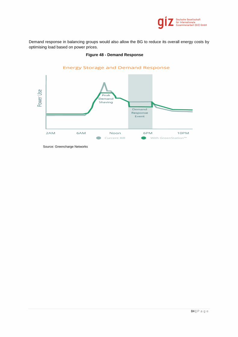
84 | P a g e
Demand response in balancing groups would also allow the BG to reduce its overall energy costs by
optimising load based on power prices.
Figure 48 - Demand Response
Source: Greencharge Networks

85 | P a g e
7 Transition to Proposed Market Design
The objective of the proposed market design is to transform India’s current power market structure
into a 100% market based system. Products like power, generation capacity and regulation reserves
would be offered by a large number of players to a large number of buyers. This is aimed at
increasing the cost efficiency of the power system. This transition is designed for a 15 year period
starting 2015. The time period for transition or its phases as mentioned may be altered as required,
however key issues to be addressed would be the same.
Certain key issues need to be addressed for a smooth transition into the proposed market design:
a) PPAs which have remaining validity between 1 month and 25 years should continue. New
PPAs for conventional generation should be restricted through a regulated procedure. During
the initial phase, long term (20 years) PPAs should be offered to RE based projects.
b) The restriction on signing of new PPAs would create the need of a reliable source of revenue
for the businesses investing in any component of the power system. Without the assurance of
revenue that a PPA offers, lending institutions will find it risky to invest in generation projects.
c) To address the issues of investment risk futures products will need to be introduced on the
power exchanges. These products would enable developers to trade in power to be
despatched up to 15 years into the future, however there will need for restrictions on %
capacity a generator can bid for the futures products.
d) Once the market has stabilised and 10 year price trends on the market are available or
earlier, futures products should be restricted to 5 years and a maximum of 1 month of
continuous generation. Players may be allowed to buy/sell consecutive products involving 2
or more months of continuous operation. These restrictions are required to maintain liquidity
in the market.
e) Defaulting on contract would lead to imbalances and a threat to system security; these would
be mitigated by the formation of balancing groups and introduction of ancillary services.
f) Ancillary service products are currently procured only from ISGS with URS. This prevents
more optimally located and possibly more economic generators from providing reserves. In
the future it is recommended that ancillary services and associated reserves also be procured
on the PXs from a pool of eligible and certified players.
g) Introduction of new products in the market as specified in Table 17
The following figure depicts the current Indian power market design.

86 | P a g e
Figure 49: Current Power Market
7.1 Phase 1
The transition to the new market will be executed in 3 Phases over 15 years. Phase 1 would take a
total of 5 years to implement and would lead to 11% or more of the power being traded on the
exchanges. It would have 3 major components:
7.1.1 Modifications to regulations related to Power Purchase Agreements
The first step to ensure that in the future all power is traded on the PXs is to prevent the signing of
new PPAs and migration of generators and consumers to the PXs as their PPAs expire. This
provision would not terminate any existing PPAs. As a result during the initiation of transition, there
will be PPAs with duration of up-to 25 years. New conventional power plants would not be allowed to
sign PPA and will have to sell all their power via the PXs. This is aimed at creating a liquid and deep
power market.
The phasing out of PPAs would reduce the bankability of power projects and the investors would not
have the financial security provided by a PPA. This can be addressed by the introduction of long term
power products on the PXs during the transition which provide assurances similar to a PPA. Owing to
the sensitive nature of the problem, as a temporary extraordinary measure the government will have
to assure minimum returns to a plant commissioned as-per norms under the new regulations. These
measures would cease to operate at the discretion of the appropriate regulatory bodies.

87 | P a g e
7.1.2 New Products in the market
To enable sale of all power on the PXs and the returns of new generators the products on the
exchanges would need to be introduced as below. The long duration products would be phased out in
later phases of the transition.
Table 17: Proposed Products on the Power Exchange
Product Time to
Dispatch
(Days)
Capacity
Step
(MW)
Price
Step
(Rs/MW)
Min no of
Continuous
time Blocks in
a day
Max No of
Continuous
time blocks in
a day
Duration
(Days)
Electricity
Futures
short
12- 30 .25 .01 4 96 1-7
Electricity
Futures
Medium
30-90 .5 .1 8 96 8-30
Electricity
Futures
year
91-365 .5 .1 8 96 8-30
Electricity
Futures
Long
366-5475
(365*15)
2 1.0 16 96 31-90
7.1.3 Introduction of Generator only Balancing Groups & Reserve Products
Generator only balancing groups would be introduced as described in this report. Reserve products
would also be introduced. There will be regional restrictions on the formation of balancing owing to
transmission constraints in the system.
The methodology of defining regions in which generators or consumers will form balancing groups
would be similar to the methodology followed during market splitting on the PXs. Market splitting is
based on transmission constraints which leads to the creation of localised markets with unique Area
Clearing Prices (ACPs) in contrast to the Market clearing Prices (MCPs)
The splitting of regions based on transmission constraints for balancing group formation would lead to
different prices for imbalance energy in each of the identified regions. The difference between
imbalance energy prices between regions of balancing group formation will be an important indicator
in the planning of transmission capacity. Transmission capacity planning in the various phases of
transition to new market would require factoring in the differences between the imbalance energy
prices of the initially identified regions
The quantum of price difference in imbalance energy will indicate the demand for transmission
capacity between the regions being compared.
The introduction of balancing groups for generators within a state would have an effect similar to intra
state DSM, however it would reduce the administrative load of the LDCs as the generators would now
be organised into balancing groups represented by BRPs and the LDCs would need to audit and
monitor only the schedules of BRPs instead of all generators individually.

88 | P a g e
7.1.4 Introduction of Generator Only Balancing Groups
This regulation would require generators interstate/intra-state to organize into balancing groups which
are represented by a Balance Responsible Party (BRP). These BRPs would aggregate the schedule
of all generators in their jurisdiction and provide it to the respective LDC as needed. The BRPs would
be financially liable for their netted deviation from schedule. The formation of balancing groups would
allow the members of a group to net their imbalances and support each other in ensuring adherence
to schedule of the group.
The BRP would pay/receive imbalance energy charges based on their deviation from schedule and
the status of the grid at the time of deviation.
Formation of balancing groups intra-state would allow the functioning of an intra-state Deviation
Settlement Mechanism, where multiple BRPs in a state would be responsible for their aggregated
schedules to the SLDC of the state.
Deviation & Settlement
Every BRP would be responsible for the deviations in their schedule. In case of imbalance due to
under generation, the BRP will bear the cost for alternative energy sourced to net the imbalance. In
case of imbalance due to over generation, BRP would receive reduced payment for the energy
generated after adjusting for the penalties. The financial settlement for the imbalance would happen
as below
a) Between BRP and SLDC
Here the BRP will pay the responsible SLDC or vice versa based on the type (+/-) of deviation
from schedule and the situation of the grid at the given time. All contracts between BRPs and
SLDCs will be standardized across the complete system. The contracts will be regulated..
b) Between BRP and Group Member
Here the penalties/incentives will be shared between the BRP and the members as agreed
upon between the parties at the time of group formation. These contracts will not be
regulated.
Deviation settlement would be done at both the intrastate and interstate levels; however the entities
participating in DSM would be balancing groups at various hierarchical levels
(National/State/Intrastate). Intrastate deviation settlement mechanism is currently operational in five
states such as Gujarat, Maharashtra, Delhi, Orissa and West Bengal.
Intra-State Deviation Settlement
The balancing groups which are formed within the jurisdiction of a single SLDC would enable the
operation of a DSM like mechanism within the state, where generators and consumers provide a
composite schedule for every 15 minutes of the next day and are financially liable for the deviations.
The introduction of this mechanism is expected to improve grid discipline within a state and resulting
in an overall improved frequency profile of the national grid. In Phase 2, Participation of consumers in
balancing groups via load forecasting and scheduling (flexible loads) is expected to improve
frequency profiles of the national grid.
The introduction of balancing groups within a state would also allow the BRPs of the various groups
formed to leverage the effect of imbalance netting and reduce the overall penalty payable due to
deviation from schedule.
Inter State Deviation Settlement
The proposed introduction of balancing groups allows generators to form balancing groups across a
singular or multiple state boundaries. These balancing groups would benefit by leveraging the netting

89 | P a g e
of imbalances and spatial smoothening of deviations due to RE (if RE generators are present in the
group). It is expected that transmission constraints would play an inhibitory role in the formation of
interstate balancing groups as they would restrict the flow of balancing energy.
Regional Restrictions
Balancing group formation would need to be restricted to regions based on transmission constraints.
The regional restrictions would be similar to the splitting of the PXs due to transmission constraints.
Each region would have different imbalance energy prices based on its generation mix. The
difference between imbalance energy prices between regions, would act as an indicator to the deficit
in transmission capacity. This difference in prices would need to be factored into transmission
planning. These regional restrictions would not be required once adequate transmission capacity is
available; as a result the imbalance energy would have a standard Market Clearing Price (MCP)
instead of multiple Area Clearing Prices (ACPs).
Mandatory Group Formation
It will be mandatory for all generators to form balancing groups within 6 months of notification of the
Act..
7.1.5 Congestion Management
Congestion Management and transmission planning will need to be modified to cater to the following:
a) Regional splitting of PXs and BGs due to transmission constraints
b) RE evacuation intrastate and interstate
c) Extra margin for open access consumers
7.1.6 Flexible Generation
Standards for all generators commissioned post notification will need to be upgraded to cater to the
flexibility required by a grid with large proportions of RE generation. These standards would need to
be at par with international best practices and will have to be revised periodically to ensure continuous
adoption of flexible and efficient generation.
In the market post completion of Phase 1 of the transition, it is expected that small percentage of the
power will be traded at the exchange as depicted in the following figure.

90 | P a g e
Figure 50: Market on complete implementation of phase 1
7.2 Phase 2
This phase of the market transition will feature 2 major milestones viz. Introduction of consumers in
balancing groups and trade of more than 50% power on the PXs post completion of phase 2. The
introduction of consumers in balancing groups would enable the introduction of demand side
management. Consumers would be incentivized to forecast loads and also provide demand response
products.
The following regulatory, policy and capacity building measures are recommended for achieving this
phase of transition:
7.3 Required Legislative and Regulatory Changes
The appropriate act / regulations may go through the required revisions over the 5 years period of
phase 1 therefore this section refers to the amendments required in the most recent revision of the
law and regulation during that time period.

91 | P a g e
7.3.1 Introduction of Consumers in Balancing Groups
The introduction of consumers in the balancing groups would create three types of balancing groups
as below:
a) Generator only groups
b) Consumer only groups
c) Generator and consumer groups
All balancing groups will be represented by BRPs. These BRPs would be responsible for the
combined schedule of the group (planned generation and forecasted load). The deviation settlement
and netting of imbalances will be followed. For more detailed description refer section 6.2.2 of Market
Design for RE Integration in India.
7.3.2 Introduction of Demand Side Products
Loads which are flexible and/or interruptible would be allowed to trade in demand side measures to
help support the grid. These loads will participate as part of balancing groups. These products would
be procured from the PXs similar to other reserve products.
7.3.3 Load Forecasting
Load forecasting should be incentivized by the introduction of consumers into balancing groups. This
would require the introduction of forecast service providers for loads. Accurate load forecasting and
management would allow a balancing group to minimize its deviations and therefore the
penalizations.
7.3.4 Review of Balancing Group Regional Restrictions
Based on the development of transmission capacity over the first phase of transition the regional
restrictions on balancing groups would need to be reviewed and removed if found unnecessary.
7.3.5 Migration of PPAs
Generators with PPAs older than 10 years at the beginning of phase 1 would migrate to the PXs by
the end of phase 2. Most generators would now have recovered their costs over 20 years as per their
PPAs. For the remaining life of the project by regulation the plant would be required to trade all its
power on the market.
The plants that were commissioned up to year 2000 would have completed a minimum of 20 years by
the beginning of phase 2 and a minimum of 25 years by the end of phase 2. As a result all plants
commissioned before 2000 (expired PPAs) and after 2015 up to 2020 would be trading all their power
on the market as existing products or new products introduced in phase 1.
The illustration below in the following figure represents the market post completion of phase 2.

92 | P a g e
Figure 51: Market structure after complete implementation of Phase 2

93 | P a g e
7.4 Phase 3
This is the final phase of the market transition. This phase does not involve extensive regulatory
measures. On completion of phase 3 all power would trade via the PXs, all reserve products and
ancillary services would also be provisioned via the PXs; however the completion of the market will
require the following:
7.4.1 Modification of Products on PXs
The long term products which were introduced in phase 1 to mitigate investor risk will now be
modified to ensure that the longest time period between trade and dispatch not to exceed 5 years (15
year products introduced in phase 1). This would be possible in phase 3 as the market would have
operated for 10 years and in this time the price trends would have been well understood by the
investors.
7.4.2 Migration of PPAs
As in phase 2 the generator who’s PPAs have expired would be required to trade all their power in the
PXs. The power markets would have operated with incrementally higher amounts of power being
traded on it for 10 years. Understanding of price patterns and returns on market based products
would have matured over this operating time. Based on this a two pronged approach may be followed
to migrate the remaining generators onto the exchange.
Optional Migration
Based on the market trends, a generator whose PPA has completed 10 years at this point would be
encouraged to dissolve these PPAs and migrate to the PXs. These generators would migrate
expecting better returns from the market than the current PPAs would offer.
Mandatory Migration
At the end of phase 3 remaining PPAs would have a maximum remaining validity of 10 years. This is
assuming it was a 25 year PPA signed 1 day before the notification of restriction on PPA regulations.
The longest permitted gap between trade and dispatch would be reduced to 5 years.
All remaining PPAs would be converted into 5 year products tradable on the exchange, if not traded
would function similar to the PPA for these 5 years. Once a PPA has completed 20 years then it
would be terminated and henceforth the parties involved would trade on the PXs only.
Exemptions
Exemptions could be made on a case to case basis up to a point where all investors have broken
even. Beyond that point all power would trade in the market.
7.4.3 Review of RPO/REC
It is estimated that by the beginning of phase 3, RE power would have become cheaper than the MCP
and RPOs/RECs may not be required. Based on the situation at the time they should be phased out.
The illustration below in fig 49 below represents the market post completion of phase 3.

94 | P a g e
Figure 52: Market on Completion of Phase 3

95 | P a g e
7.5 Proposed Market Design for India
In view of the upcoming capacity addition plans for both conventional and RE power, it is proposed
that the Indian power market should develop a perfectly competitive wholesale market. Such a market
should provide liquidity and prevent abuse of market power by some players in the market. Because
RE generation will form a sizable portion of the total power generation mix in India in the near future,
there is a need to ensure the off take of RE power and make it schedulable. The following are the key
considerations for designing a perfectly competitive wholesale generation market for the Indian
scenario.
Ensure enough liquidity in the market
Control each participant’s ability to exert market power
Trade of all power through cost based bids based on predetermined variable costs of
generation
MUST RUN status for RE power to be ensured by the merit order in the market
7.5.1 Market Design
Keeping the above key considerations in mind, it is proposed that the Indian power market should
move to a two-sided cost based gross pool. Under such an arrangement all power in the Indian
power market would be traded at the power exchange. A graphical representation of the proposed
market design is given in the following figure.
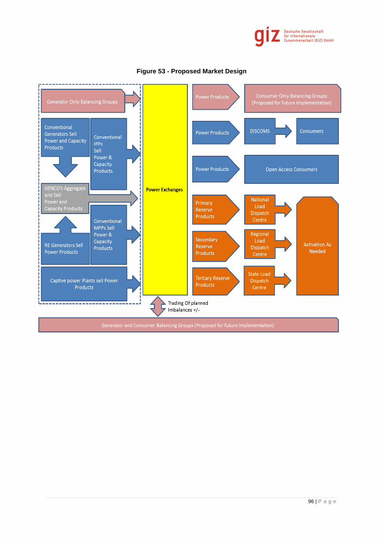
96 | P a g e
Figure 53 - Proposed Market Design
97 | P a g e
Market Description
Under the proposed market setup, all the power producers would be required to sell their generation
on the power exchange. No sale of power would then happen through direct bilateral arrangements
between power producers and consumers. It is proposed that with immediate effect, no new PPAs
should be signed and the existing PPAs should be allowed to phase out as per existing contracts to
move from the existing system to a completely exchange based power market. In case any PPAs
have to be scrapped, the regulator has to make provisions for debt restructuring.
The state GENCOs will be responsible for aggregating power from all RE generators under their
jurisdiction and selling it on the exchange. The conventional generators who do not fall under the
jurisdiction of the GENCOs and captive power plants would sell their power directly at the exchange.
All conventional generators would be remunerated as per the market clearing price for the time block
their power is sold at the power exchange.
The DISCOMs would be required to bid for power at the power exchange for every time block as per
their scheduled demand. The DISCOMs would therefore be responsible to demand forecast for each
time-block to be able to accurately schedule their demand.
Way forward to achieve the proposed market design
In order to enable the transition to an exchange only power market, the Indian power market has to be
restructured to redistribute roles as proposed, address transmission constraints, prepare for upcoming
RE capacity addition and address all the concerns highlighted in Section 1 of this report.
It is proposed that as the first step, the regulators should introduce mandates for the creation of
Balancing Groups and set up of Control Reserves for provisioning of ancillary and balancing services
as described in the following sections.
Players in the power market should be given a lead time – as decided by the regulators – to organise
themselves into balancing groups. Players, who are unable to form a balancing group within the lead
time, should provide suitable justification for the same. These market players should be penalised or
allowed to buy/sell power directly from the exchange as per the discretion of the responsible
regulators.
Pricing Model
There should be a gradual move to the cost based pricing model once balancing group
arrangement has stabilised, the planned transmission capacity has been implemented and all power
can be sold at the exchange. Under this pricing regime, the conventional generators’ bids will be
based on the best price the generator can offer (including price to recover capex and opex, and profit)
given time block. RE power should be bid at marginal cost to generator which would ensure that RE
power (with minimal marginal costs) will be the first in the merit order to be scheduled for dispatch.
Market Products
Since the cost based pricing model does not provide signals for long-term investment, a new long
term market product should be introduced at the exchange that would help provide long term price
clarity for consumers. All generators that meet requirements should be able to bid not only energy but
their unscheduled capacity for the provision of control reserves.

98 | P a g e
7.6 Deviation and mechanism of settlement
The deviations from schedule of balancing groups would be penalised if they are destabilising the
grid, however they will be incentivised for stabilising the grid. It is recommended that 100% adherence
to schedule should also be incentivised.
Regulatory funds would need to be created at the national, regional, state levels.
National Fund - This fund would be created from the penalty paid by the regional entity for their
unscheduled imbalances and would be used to compensate the regional entities which adhere to
schedule. The penalties would be charged from and the incentives will be deposited in the respective
regional funds.
Regional Fund - This fund would be created from the penalty paid by the state entity for their
unscheduled imbalances and would be used to compensate the state entities which adhere to
schedule within a regional balancing group. The penalties would be charged from and the incentives
will be deposited in the respective state funds.
State Fund - This fund would be created from the penalty paid by the zonal entity for their
unscheduled drawls/injections and would be used to compensate the zonal entities which adhere to
schedule. The penalties would be charged from and the incentives will be deposited in the respective
Zonal funds.
The system security would be managed by using ancillary and balancing reserves.
Management of Schedule Deviations due to RE
All RE power would be purchased by the GENCOs at prices discovered through competitive bidding
process. This would mean that by default the GENCOs would aggregate RE and manage the
imbalance caused due to the variability in RE generation, all RE generators would be a part of the
GENCOs balancing group. The cost of imbalance energy for the permitted deviation of RE (revised
from time to time by regulatory commissions) would need to be socialised as it would be an additional
burden on the GENCO. The deviation due to RE over and above the permitted range would need to
be managed by the generators/consumers in the GENCOs balancing group. Deviations from
schedule above permitted band would be penalised if not mitigated within the group. This penalisation
would compensate the reserve service providers for the balancing energy they supply.
The GENCOs may further pass on this imbalance cost to the RE generator(s) on a pro rata basis of
their individual deviations from schedule.
Remuneration to RE Generators and Aggregators
The price paid per unit to RE generators would be the price discovered via bidding. This per unit price
would be paid to the generator by the GENCOs in the proposed scenario. The GENCOs would
receive the MCP for the units sold and the difference between the bid price and MCP per unit would
need to be socialised.
It is expected that in the future the MCP received per unit of RE power would be more than the bid
price of RE. In this situation a percentage of the profits that GENCOs make on sale of RE power on
the market should be passed on to RE generators after accounting for the imbalance charges if any.

99 | P a g e
7.7 Control Reserves (Ancillary Services and Balancing)
Control reserves are a critical part of the power system and are mandatory for managing large scale
RE grid integration. These reserves are required for the delivery of balancing services and Frequency
Control Ancillary Services.
7.7.1 Contracting of reserves
The reserves will be contracted in a three tier system where
Primary reserves will be contracted by the NLDC
Secondary Reserves will be contracted by the RLDC
Tertiary reserves will be Contracted by the SLDC
This hierarchical placement of reserves will ensure that conflicting activation of reserves does not take
place. Over compensation to frequency correction would also destabilise the system.
The method for estimating the quantum of reserves required and their positioning is covered under
the reserve dimensioning section of this report.
Restriction on capacity contracted per provider
The contracting of reserves will have to be done keeping in mind that no single provider should be
allowed to bid for more than a small fraction of the reserves required in the time block. This is to
ensure that the failure of the provider affects only a small fraction of the available reserve and reduces
the risk of the reserve failing altogether due to the failure of a large provider. This will also incentivise
a larger number of players to upgrade and participate in the market for these reserves.
Distribution of reserves:
To prevent inter regional power flows due to reserve activation, The NLDC, RLDC and SLDC would
need to ensure that the contracted reserves are distributed all over the control regions and activation
does not lead to large inter control region power flows, in a case of grid congestion the reserve might
be rendered ineffective and further deteriorate the frequency condition. The estimation of the quantum
of reserves required in every control region would need to be done based on the reserve
dimensioning and the scheduled power flows.
7.7.2 Scheduling of reserves
The scheduling of availability of reserves will be done for each of the 96 time blocks; however
dispatch is function of need based on contingencies as they arise. Each of the three reserves would
be scheduled as below.
Primary Reserves
Capacity as required and estimated by the NLDC for every time block would be contracted at latest in
the day ahead market, any corrections to this contracted capacity could be done in the intra-day
contingency market. These reserves do not have a scheduled dispatch; however they have a
scheduled availability. They are implemented by the simultaneous action of FGMO in plants which
have been contracted for the purpose in the time block.
Secondary Reserves
Capacity as estimated by the RLDCs for their respective control regions in every time block would be
contracted through the term ahead, day ahead and Intraday contingency markets for each of the 96

100 | P a g e
time blocks. The despatch of this capacity is not planned and is triggered by a frequency excursion
(+/-). These reserves are used to restore the frequency after its change has been arrested by the
primary reserve activation.
Tertiary Reserves
These are the only reserves whose dispatch is a part of the schedule, the purpose of tertiary reserves
is to continue the action of primary reserves. They are required to reach 100% output in 15 mins from
activation. These reserves are included as a part of the schedule for the time blocks they are
activated for. Currently the Indian power system has only tertiary control available. Regulations for the
introduction of primary and secondary reserves have not been notified yet.
7.7.3 Activation of Reserves
These reserves are contingency measures and their activation is required to correct a change in
frequency, their activation is needed when there is a deviation from schedule by either a generator or
consumer. A system fault like the tripping of a line section may also result in the activation of control
reserves to manage the imbalance caused by the fault.
The activation of reserves is a seamless process. The activation of primary reserves is to arrest the
change in frequency and is required to react immediately, Secondary control is activated within 30
seconds and reaches full load within 5 minutes, and the tertiary reserve is activated in 5 minutes and
reaches full load in 15 mins, tertiary reserve sustains the secondary reserve till needed. This ensures
that primary reserves are freed up by the activation of secondary reserves and the activation of
tertiary reserves frees up the secondary reserves.
Primary reserves: This reserve is automatically activated based on a pre-set frequency range; it
does not feature in the dispatch schedule as it is an emergency measure to correct a deviation from
schedule. They will be controlled by the NLDC and will be used to arrest the change in frequency.
These reserves will need to reach full capacity within 30 seconds and start acting immediately after
the fault.
Secondary Reserves: These reserves can be either manually or automatically activated. They will be
activated by the RLDC within 30 seconds and would need to reach full load within 5 mins. These
reserves are used to correct the frequency after its change has been arrested by the primary
reserves.
Tertiary reserves: These reserves are manually activated. They will be activated by the SLDC, these
reserves would be activated within 5 mins and would need to reach full load within 15 minutes of
activation. The duration of activation of these reserves would be up-to 8 time block or higher as
needed for safe, secure and reliable power system operation.
7.7.4 Infrastructure for Deployment of Reserves
The activation of reserves is a very critical and technology intensive process. The various control
reserves as described above would need the following infrastructure for their implementation.
Primary Reserves: These providers will be contracted by the NLDC; the activation of these reserves
is automatic and is achieved by setting the governors of plants providing these reserves to FGMO.
The droop settings of the governors would need to be as-per the frequency bands set in IEGC.
Certain primary response measures would also require setting up of communication and control
infrastructure between the NLDC and the reserve service provider. This needs to be done in order to

101 | P a g e
achieve automatic activation of the reserves. If not activated automatically the NLDC would need to
activate these reserves under 30s.
Secondary Reserves: These providers would be contracted by the respective RLDC’s. These
reserves in an ideal case would be activated automatically. Their activation would be 30s after the
triggering of primary reserves. The technical requirements for their implementation require AGC. The
RLDC would need to have AGC enabled and online reserve service providers contracted. If the
activation is not automatic, protocols for quick manual intervention would need to be setup as the
reserves need to attain full required capacity under 5 minutes.
Tertiary Reserves: These reserves are activated by the SLDC and may or may not have automatic
activation. These reserves would need to be triggered within 5 minutes and ramped up/down to
required capacity within 15 minutes. India currently has only tertiary control measures in place.
7.7.5 Payment to reserve service providers
Primary Reserves: Primary reserves would be contracted and activated (If not done automatically)
by the NLDC. The NLDC would contract only capacity for the primary reserves. In India this cost
should be recovered by socializing it among the balancing groups pro rata based on their portfolio
size.
Secondary Reserves: Secondary reserves would be contracted by the RLDCs for their respective
control areas. The activation (if not automatic) of the secondary reserve would be the responsibility of
the RLDC. The Power provision will be tuned by the RLDC with intra-state exchange schedules to
account for any congestion (described in section named "grid control cooperation"). For secondary
control both, power and energy are contracted. This remuneration of energy costs have to be settled
together with SLDCs. With reference to the provisions proposed for primary control above the
component of cost that is paid for contracting the reserve would be socialized as above. The cost of
actual energy used to handle the imbalance would be borne by the BRP responsible for the deviation
after netting their imbalances.
Tertiary Reserves: These reserves would be contracted by the SLDCs. The activation control and
monitoring of these reserves would be under the jurisdiction of the SLDC. For tertiary reserves both
capacity and energy is contracted. The capacity contracted is paid for by socialization of the costs as
above. The cost for the actual energy required would be paid for by the balancing group responsible
for the netted imbalance.
7.7.6 Reserve service providers
The reserve service providers would be any players in the market who can adhere to the below
mentioned requirements. The table below mentions the activation time, reaction time and time to
complete activation of the various control reserves. The eligibility of a reserve service provider would
be certified by the CEA and will be reviewed regularly. The CEA would need to define technology and
provider neutral standards for each type of reserve providers.

102 | P a g e
Table 18: Requirement of Different types of control reserves
Primary control
reserve
Secondary control reserve Tertiary control reserve
Purpose Stabilize grid frequency
after a disturbance
Balance control areas, bring grid
frequency back to nominal value,
replace primary control
Complement and replace
secondary control
Time until
complete
activation
30 sec 5 min 15 min
Reaction time immediately 5 min, 30 sec until first change of
power for pooled reserve providers23
15 min
Activation Local, static relation
to the frequency
Immediately by the TSO via set
points
Automatically by Merit
Order List Server (MOLS)
7.7.7 Penalty for defaulting reserve providers
The default of a reserve service provider would mean that a fault occurred and the activated reserve
provider did not deliver, further worsening the stability of the grid. It is recommended that a penalty
structure be put into place so that it covers the cost of activating a more expensive reserve and a
disincentive over and above.
23 Pools providing secondary control reserve have to show a first reaction to the secondary control activation signal of the TSO
within 30 seconds, at the latest.

103 | P a g e
8 Roadmap and Summary of Recommendations
The proposed market design requires complete overhaul of the existing Indian power market. The
following action points should be undertaken to develop a perfectly competitive wholesale market
where all power can be openly traded at the power exchange.
8.1 Immediate Steps – Over the next 5 years (Phase 1 of transition)
i) To ensure all power is sold on the exchange – Phasing out of PPAs and replacement
with equivalent long term products in the PXs to be made with immediate effect. The
generators with existing PPAs should be allowed to trade power as per their contract till
their PPAs phase out.
Regulators need to consider the impact of this mandate. To promote new power
generation capacity addition (both conventional and RE) new financing schemes have
to be introduced. Financing available to developers under these schemes have to take
into account the risk of sale of power in a completely competitive wholesale market.
All new generators should either sell their power directly at the power exchange or
through the GENCOs if they fall under their jurisdiction. Once the existing PPAs phase
out, GENCOs should sell all their power at the exchange.
Long term energy products can be made available at the exchange market to ensure
price clarity for large consumers and generators
ii) To ensure grid stability and to account for deviation from schedule - Balancing
groups should be created. The functioning of balancing groups and the mechanism for
commercial settlement for deviation from schedule should be introduced as explained in
the above section. In the first phase generator only balancing groups would be
introduced.
iii) To provide ancillary and balancing services - Introduction of Control Reserves
through capacity products besides energy only products on the power exchange.
The details for deployment of these reserves are explained in the above sections.
iv) Introduction of long term products on the market with despatch up to 15 years from the
date of trade
8.2 Steps to be taken after 5 years up to 10 years (Phase 2 of transition)
i) Migration to PXs: Generators with PPAs older than 10 years at the beginning of phase 1
would migrate to the PXs by the end of phase 2. By the completion of phase 2 significant
power trade in India would happen over the power exchanges.
ii) Introduction of Consumers in balancing groups: This measure will ensure the
participation of consumers in the matching of generation and load. Introduction of
consumers in balancing groups would incentivise demand response measures in
schedule management.

104 | P a g e
iii) To ensure RE power is scheduled – All the bids for sale of RE power at the
exchange to be based on marginal price incurred by generators. The bids for
conventional generators will be based on best possible price that can be offered by them.
This will ensure RE power will be first in the merit order and always scheduled first.
iv) Functioning of DISCOMs – DISCOMs should purchase power from the exchange to
meet their scheduled/unscheduled demand. In order to avoid payment for deviation
from schedule, all DISCOMs should introduce accurate load forecasting either via
external service providers or internally.
v) Modification of long term products (introduced in phase 1) on the exchange
restricting the time period between trade and despatch to a maximum of 10 years
8.3 Steps to be taken after 10 years up to 15 years (Phase 3 of transition)
i) Migration to market: All power would be traded on the exchanges by the end of phase
3.
ii) Balancing groups: All power would be sold on the exchange or purchased off the
exchange by balancing groups only. The concept of balancing groups and their operation
is covered in detail in this report.
iii) Modification of long term products (introduced in phase 1) on the exchange
restricting the time period between trade and despatch to a maximum of 5 years

105 | P a g e
9 Bibliography
Performance of Solar Plants in India. (2011, Feb). Retrieved May 15, 2015, from
http://www.cercind.gov.in/2011/Whats-
New/PERFORMANCE%20OF%20SOLAR%20POWER%20PLANTS.pdf
Perspective Transmission plan for 20 years 2014-34. (2014). Retrieved May 2015, from
http://www.cea.nic.in/reports/powersystems/sppa/scm/allindia/notices/3rd_report.pdf
38.02.08, C. T. (1995). Long-Term Dynamics: Phase II, CIGRE Technical Brochure No. 102.
A. Kurita, H. O. (1993). Multiple time-scale dynamic simulation. IEEE Trans.Power Syst., 8, 216-223.
Akhmatov, V., Rasmussen, C., Borre Eriksen, P., & Pedersen, J. (2007). Technical Aspects of Status
and Expected Future Trends for Wind Power in Denmark. Wind Energy(10), 31-40.
Akshay Urja, M. (n.d.). Retrieved April 2015, from http://mnre.gov.in/file-manager/akshay-urja/january-
february-2015/EN/files/basic-html/page5.html
Authority, C. E. (2013, November). Large Scale Grid Integration of Renewable Energy Sources - Way
Forward. Retrieved May 1, 2015, from
http://www.cea.nic.in/reports/powersystems/large_scale_grid_integ.pdf
Authority, C. E. (2013, Novenber). Large Scale Grid Integration of Renewable Energy Sources - Way
Forward. Retrieved March 2015, from
http://www.cea.nic.in/reports/powersystems/large_scale_grid_integ.pdf
Authority, C. E. (2015, May 31). All India Installed Capacity (in MW) of Power Stations (As on
31.05.2015). Retrieved June 15, 2015, from
http://www.cea.nic.in/reports/monthly/inst_capacity/may15.pdf
Authority, C. E. (2015, June). All India Installed Capacity (in MW) of Power Stations as on 31.05.2015.
Retrieved June 20, 2015, from http://www.cea.nic.in/reports/monthly/inst_capacity/may15.pdf
Authority, C. E. (2015, May). Load Generation Balance Report 2015-16. Retrieved June 1, 2015, from
http://www.cea.nic.in/reports/yearly/lgbr_report.pdf
CEA. (2010). Indian Electricity Grid Code. Central Electricity Authority.
CEA. (2013, April). Introduction to Ancillary Services. Retrieved May 12, 2015, from
http://www.cercind.gov.in/2013/whatsnew/SP13.pdf
CEA. (2015, January 31). All India Installed Capacity. (CEA) Retrieved from
http://www.cea.nic.in/reports/monthly/inst_capacity/jan15.pdf
CEA. (2015, February 28). Allocation of Power From Central Generating Stations to Southern Region
as on 28.02.15. Retrieved May 2015, from
http://www.cea.nic.in/reports/monthly/gm_div_rep/power_alloc_sr.pdf
Commission, C. E. (2013, April 10). Staff paper on Introduction of Ancillary Services in Indian
Electricity Market. Retrieved March 2015, from
http://www.cercind.gov.in/2013/whatsnew/SP13.pdf
106 | P a g e
Commission, C. E. (2014, September). Staff Paper on Transmission Planning, Connectivity, Long
/Medium Term Open Access And Other Related Issues. Retrieved April 2015, from
http://www.cercind.gov.in/2014/draft_reg/staff_paper.pdf
Commission, C. E. (2015, January 2). Determination of Point of Connection (PoC) rates and
transmission losses for the period January to March, 2015. Retrieved April 2015, from
http://posoco.in/Uploads/PoC%20Rates%20and%20Losses%20Order%20for%20Jan15-
Mar15%20(Q4).pdf
Commission, G. E. (n.d.). 15 Annual Report FInancial Year 2013-14. Retrieved May 2015, from
http://www.gercin.org/reportpdf/en_1434108536.pdf
Commission, H. P. (n.d.). Annual Administrative Report 2013-14. Retrieved May 2015, from
http://www.hperc.org/aare13-14.pdf
Commission, P. (August 2006). Integrated Energy Policy, Report of Expert Committee. New Delhi:
Government of India.
CWET. (n.d.). India's Wind Power Potential. Retrieved May 05, 2015, from http://mnre.gov.in/file-
manager/UserFiles/Presentations-NWM-09012014/Gomathinaygam.pdf
Dr Alex D Papalexopoulos, D. G. (2012). Reactive power management and pricing in california power
markets. Retrieved May 12, 2015, from ECCO internation INC:
http://www.eccointl.com/downloads/Reactive-Power-Management-and-Prcinig-in-the-
California-Market.pdf
EirGrid. (2010). 2010-11 Harmonised Ancillary Service Statement of Payments and Charges.
Retrieved April 2, 2014 , from
http://www.eirgrid.com/media/2010%202011%20Harmonised%20Ancillary%20Service%20St
atement%20of%20Payments%20and%20Charges.pdf
EirGrid. (2010, October 1). Ancillary Service and Other Service Chargest Example Calcuator.
Retrieved April 14, 2014, from
http://www.eirgrid.com/operations/ancillaryservicesothersystemcharges/
EirGrid. (2013, October 7). Grid Code Version 5.0. Retrieved April 4, 2014, from
http://www.eirgrid.com/media/GridCodeVersion5.pdf
EirGrid and SONI. (2013, August 7). Operational Constraints Update 7th August 2013. Retrieved April
1, 2014, from
http://www.eirgrid.com/media/OperationalConstraintsUpdate_v1.8_August2013.pdf
Energy Department, G. o. (2014). Policy Note 2014-2015. Retrieved May 2015, from
http://www.investingintamilnadu.com/files/whats_new_docs/Energy_Policy_Note_2014_15.pd
f
Energy, M. o. (2012, December). Jawaharlal Nehru National Solar Mission Phase II – Policy
Document. Retrieved April 2015, from http://mnre.gov.in/file-manager/UserFiles/draft-
jnnsmpd-2.pdf
ENTSO-E. (2015). Systems operations Committee. Retrieved from ENTSO:
https://www.entsoe.eu/about-entso-e/system-operations/Pages/default.aspx

107 | P a g e
European Wind Energy Agency. (2004). Large Scale Integration of Wind Energy in the European
Power Supply: analysis, issues and recommendations: Electrical grids and wind power: the
present situation in Europe. Retrieved April 15, 2014, from
http://www.ewea.org/fileadmin/ewea_documents/images/publications/grid/AAA-
_countries_study_4_Final.pdf
FICCI. (2013, September). Power Transmission - The Real Bottleneck. Retrieved April 2015, from
http://www.ficci.com/spdocument/20311/power-transmission-report_270913.pdf
FICCI. (September 2013). Power Transmission , The Real Bottleneck. FICCI.
Giebel, G., Sorensen, P., & Holttinen, H. (2007, April). Forecast error of aggregated wind power.
Retrieved April 15, 2014, from http://www.trade-
wind.eu/fileadmin/documents/publications/D2.2_Estimates_of_forecast_error_for_aggregated
_wind_power_Final.pdf
Global Wind Energy Council, World Institute of Sustainable Energy, Indian Wind Turbine
Manufacturing Association. (2012, November ). India WInd Energy Outlook 2012. Retrieved
May 2015, from http://www.gwec.net/wp-content/uploads/2012/11/India-Wind-Energy-
Outlook-2012.pdf
Gujarat Energy Development Agency, G. (2013, January). Renewable Energy Scenario in Gijarat.
Retrieved March 2015, from http://geda.gujarat.gov.in/media/2.REJan2013.pdf
Hayden, M. (2011, July 7). Using Forecasts and Dispatching Wind from NCC. Retrieved April 15,
2014, from www.eirgrid.com/media/Power%20System%20Seminar%204.pdf
HIMURJA. (n.d.). Small Hydro Development Programme in Himachal Pradesh. Retrieved May 2015,
from http://himurja.nic.in/smallhydro.html
Holttinen, H., Meibom, P., Orths, A., van Hulle, F., Lange, B., O'Malley, M., et al. (2009). Design and
operation of power systems with large amounts of wind power. International Energy Agency
Wind Task 25.
IMO and System Management. (February 2014). Load Following Ancillary Service Monitoring
Specification. Perth.
IMO and System Management. (October 2013). LFAS Requirement Investigation: Analysis of LFAS
causes and usage. Perth.
India, B. t. (2014, May). India’s solar installed capacity crossed 2.5 GW in May 2014. Retrieved April
2015, from http://www.bridgetoindia.com/blog/indias-solar-installed-capacity-crossed-2-5-gw-
in-may-2014/
International Renewable Energy Agency. (2014). REthinking Energy: Towards a new power system.
Retrieved March 15, 2015, from
www.irena.org/rethinking/Rethinking_FullReport_web_print.pdf
Invest, R. (2015, January). Investors Guide Re-invest 2015. Retrieved May 2015, from http://www.re-
invest.in/Document/orginal/15.RE-Invest_2015_Investors_Guide.pdf
IRENA. (2013, April 16). Integrated Renewable Energy Resource Assessment for Gujarat. Retrieved
April 2015, from

108 | P a g e
http://www.irena.org/menu/..%5CDocumentDownloads%5Cevents%5CDelhiEvent%5C1.5%2
0TERI%20Gujarat%20RE%20Atlas.pdf
Kundur, P. (1994). Power System Stability and Control. New York, USA: McGrawHill.
Kyri Baker, T. S. (n.d.). Model Predictive Control of a Steam Turbine. United States: Carnegie Mellon
University.
Limited, K. P. (n.d.). KPCL Power Projects in Karnataka. Retrieved May 2015, from
http://karnatakapower.com/wp-content/uploads/2014/06/kpcl_project_details-2014.xls1.pdf
Limited, P. S. (2015, January 19). Operational Feedback on Transmission Constraints: January 2015.
Retrieved April 2015, from
http://posoco.in/attachments/article/87/NLDC_Operational_Feedback_January%202015.pdf
Line, B. (2014, December 23). Allow open access to power: panel. Retrieved May 2015, from
http://www.thehindubusinessline.com/economy/allow-open-access-to-power-
panel/article6719841.ece
Ltd., K. R. (2015, February). Progress on RE commissioned capacity by February 2015. Retrieved
April 2015, from http://kredlinfo.in/reprogressreport.aspx
Ltd., M. E. (November 2012). Integrating Variable Renewable Energy with the Grid: Lessons from the
Southern Region. Sustainable Energy Foundation.
Mehebub Alam, S. M. (October 2014). Renewable Energy Sources (RES): An Overview with Indian
Context. International Journal Of Engineering And Computer Science, 3(10), 8871-8878.
Milligan, M., & Kirby, B. (2010). Market Characteristics for Efficient Integration of Variable Generation
in the Western Interconnection. NREL.
Ministry of Power, G. o. (2012, January). Report of The Working Group on Power for Twelfth Plan
(2012-17). Retrieved April 2015, from
http://planningcommission.nic.in/aboutus/committee/wrkgrp12/wg_power1904.pdf
Ministry of Power, Government of India. (2015, March 27). Scheme for Utilization of Gas based Power
Generation Capacity. Retrieved June 15, 2015, from
http://powermin.nic.in/upload/Scheme_for_utilization_of_Gas_based_power_generation_capa
city.pdf
MNRE. (2014, November 24). State wise Estimated Solar Power Potential in the Country. Retrieved
April 2015, from http://mnre.gov.in/file-manager/UserFiles/Statewise-Solar-Potential-NISE.pdf
MNRE. (2015). Indian Renewable Energy and Energy Efficiency Policy Database - Renewable
Purchase Obligation 2014-15. Retrieved May 1, 2015, from http://ireeed.gov.in/statepolicy#
MNRE. (n.d.). Frequently Asked Questions (FAQs) on Biomass Power Generation. Retrieved May 15,
2015, from http://mnre.gov.in/file-manager/UserFiles/faq_biomass.htm
National Grid. (2013, October). Wind Generation Forecasting. Retrieved April 15, 2014, from
www2.nationalgrid.com/UK/Industry-information/Electricity-system-operator-incentives/wind-
generation-forecasting/

109 | P a g e
Planning, Programme Monitoring and Statistics Department, Government of Karnataka. (20114).
Economic Survey of Karnataka 2013-14. Retrieved March 2015, from
http://planning.kar.nic.in/docs/economic%20survey%202013-
14/Web%20Eng/20%20ECONOMIC%20INFRASTRUCTURE.pdf
Power, M. o. (2011). One Day Workshop on PoC Charges Regime. Government of India. New Delhi.
Riesz, J., Gilmore, J., & Hindsberger, M. (2013). Market design for the integration of variable
generation. In F. P. Sioshansi, Evolution of global electricity markets (p. 757). Academic
Press.
Saadat, H. (n.d.). Power System Analysis.
SKM. (2010 , August 5). Intermittent Generation Penetration within the Wholesale Electricity Market.
Retrieved from IMO: http://www.imowa.com.au/docs/default-source/Governance/Market-
Advisory-Committee/MAC-Working-Groups/final_wp4_technical_rules.pdf?sfvrsn=2
Standard, B. (2014, July 18). Accelerated Depreciation scheme for wind energy restored. Retrieved
March 2015, from http://www.business-standard.com/article/news-ians/accelerated-
depreciation-scheme-for-wind-energy-restored-114071800777_1.html
Urja, A. (2011, October). RePowering Wind Farms in India. Retrieved May 15, 2015, from
http://mnre.gov.in/file-manager/akshay-urja/september-october-
2011/EN/RePowering%20Wind%20Farms.pdf
Western Power. (2011, December 23). Technical Rules. Retrieved April 28, 2014, from Economic
Regulatory Authority Website:
http://www.erawa.com.au/cproot/10353/2/20120504%20Western%20Power%20Technical%2
0Rules.pdf
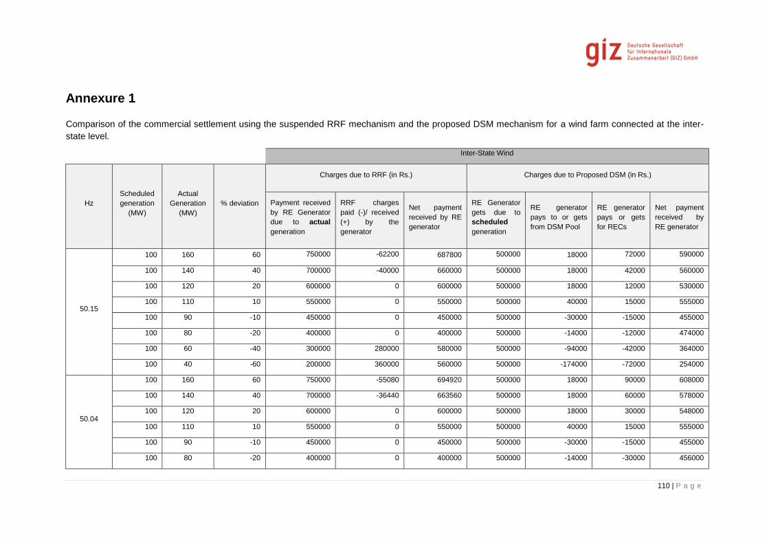
110 | P a g e
Annexure 1
Comparison of the commercial settlement using the suspended RRF mechanism and the proposed DSM mechanism for a wind farm connected at the inter-
state level.
Inter-State Wind
Hz
Scheduled
generation
(MW)
Actual
Generation
(MW)
% deviation
Charges due to RRF (in Rs.) Charges due to Proposed DSM (in Rs.)
Payment received
by RE Generator
due to actual
generation
RRF charges
paid (-)/ received
(+) by the
generator
Net payment
received by RE
generator
RE Generator
gets due to
scheduled
generation
RE generator
pays to or gets
from DSM Pool
RE generator
pays or gets
for RECs
Net payment
received by
RE generator
50.15
100 160 60 750000 -62200 687800 500000 18000 72000 590000
100 140 40 700000 -40000 660000 500000 18000 42000 560000
100 120 20 600000 0 600000 500000 18000 12000 530000
100 110 10 550000 0 550000 500000 40000 15000 555000
100 90 -10 450000 0 450000 500000 -30000 -15000 455000
100 80 -20 400000 0 400000 500000 -14000 -12000 474000
100 60 -40 300000 280000 580000 500000 -94000 -42000 364000
100 40 -60 200000 360000 560000 500000 -174000 -72000 254000
50.04
100 160 60 750000 -55080 694920 500000 18000 90000 608000
100 140 40 700000 -36440 663560 500000 18000 60000 578000
100 120 20 600000 0 600000 500000 18000 30000 548000
100 110 10 550000 0 550000 500000 40000 15000 555000
100 90 -10 450000 0 450000 500000 -30000 -15000 455000
100 80 -20 400000 0 400000 500000 -14000 -30000 456000

111 | P a g e
100 60 -40 300000 255080 555080 500000 -94000 -60000 346000
100 40 -60 200000 327960 527960 500000 -174000 -90000 236000
Hz
Scheduled
generation
(MW)
Actual
Generation
(MW)
% deviation
Charges due to RRF (in Rs.) Charges due to Proposed DSM (in Rs.)
Payment received
by RE Generator
due to actual
generation
RRF charges
paid (-)/ received
(+) by the
generator
Net payment
received by RE
generator
RE Generator
gets due to
scheduled
generation
RE generator
pays to or gets
from DSM Pool
RE generator
pays or gets
for RECs
Net payment
received by
RE generator
50
100 160 60 750000 -26600 723400 500000 18000 90000 608000
100 140 40 700000 -22200 677800 500000 18000 60000 578000
100 120 20 600000 0 600000 500000 18000 30000 548000
100 110 10 550000 0 550000 500000 40000 15000 555000
100 90 -10 450000 0 450000 500000 -30000 -15000 455000
100 80 -20 400000 0 400000 500000 -14000 -30000 456000
100 60 -40 300000 155400 455400 500000 -94000 -60000 346000
100 40 -60 200000 199800 399800 500000 -174000 -90000 236000
49.8
100 160 60 750000 57480 807480 500000 18000 90000 608000
100 140 40 700000 19840 719840 500000 18000 60000 578000
100 120 20 600000 0 600000 500000 18000 30000 548000
100 110 10 550000 0 550000 500000 40000 15000 555000
100 90 -10 450000 0 450000 500000 -30000 -15000 455000
100 80 -20 400000 0 400000 500000 -14000 -30000 456000
100 60 -40 300000 -138880 161120 500000 -94000 -60000 346000
100 40 -60 200000 -178560 21440 500000 -174000 -90000 236000
49.7
100 160 60 750000 102600 852600 500000 18000 90000 608000
100 140 40 700000 42400 742400 500000 18000 60000 578000
100 120 20 600000 0 600000 500000 18000 30000 548000
100 110 10 550000 0 550000 500000 40000 15000 555000
100 90 -10 450000 0 450000 500000 -30000 -15000 455000

112 | P a g e
100 80 -20 400000 0 400000 500000 -14000 -30000 456000
100 60 -40 300000 -296800 3200 500000 -94000 -60000 346000
100 40 -60 200000 -381600 -181600 500000 -174000 -90000 236000
Comparison of the commercial settlement using the suspended RRF mechanism and the proposed DSM mechanism for a solar plant connected at the inter-
state level.
Inter-State Solar
Hz
Scheduled
generation
(MW)
Actual
Generation
(MW)
%
deviation
Charges due to RRF (in Rs.) Charges due to Proposed DSM (in Rs.)
Payment
received by RE
Generator due
to actual
generation
RRF charges
paid (-ve) /
received (+ve)
by the generator
Net payment
received by RE
generator
RE Generator gets due to
scheduled generation
RE generator
pays to (-ve) or
gets from (+ve)
the DSM Pool
RE generator
pays (-ve) or
gets (+ve) for
RECs
Net payment
received by RE
generator
50.1
5
100 160 60 1050000 0 1050000 700000 18000 210000 928000
100 140 40 980000 0 980000 700000 18000 140000 858000
100 120 20 840000 0 840000 700000 18000 70000 788000
100 110 10 770000 0 770000 700000 40000 35000 775000
100 90 -10 630000 0 630000 700000 -30000 -35000 635000
100 80 -20 560000 0 560000 700000 -14000 -70000 616000
100 60 -40 420000 0 420000 700000 -94000 -140000 466000
100 40 -60 280000 0 280000 700000 -174000 -210000 316000
50.0
4
100 160 60 1120000 0 1120000 700000 18000 210000 928000
100 140 40 980000 0 980000 700000 18000 140000 858000
100 120 20 840000 0 840000 700000 18000 70000 788000
100 110 10 770000 0 770000 700000 40000 35000 775000
100 90 -10 630000 0 630000 700000 -30000 -35000 635000

113 | P a g e
100 80 -20 560000 0 560000 700000 -14000 -70000 616000
100 60 -40 420000 0 420000 700000 -94000 -140000 466000
100 40 -60 280000 0 280000 700000 -174000 -210000 316000
Hz
Scheduled
generation
(MW)
Actual
Generation
(MW)
%
deviation
Charges due to RRF (in Rs.) Charges due to Proposed DSM (in Rs.)
Payment received
by RE Generator
due to actual
generation
RRF charges
paid (-ve) /
received (+ve)
by the generator
Net payment
received by
RE generator
RE Generator
gets due to
scheduled
generation
RE generator pays to
(-ve) or gets from
(+ve) the DSM Pool
RE generator pays (-
ve) or gets (+ve) for
RECs
Net payment
received by RE
generator
50
100 160 60 1120000 0 1120000 700000 18000 210000 928000
100 140 40 980000 0 980000 700000 18000 140000 858000
100 120 20 840000 0 840000 700000 18000 70000 788000
100 110 10 770000 0 770000 700000 40000 35000 775000
100 90 -10 630000 0 630000 700000 -30000 -35000 635000
100 80 -20 560000 0 560000 700000 -14000 -70000 616000
100 60 -40 420000 0 420000 700000 -94000 -140000 466000
100 40 -60 280000 0 280000 700000 -174000 -210000 316000
49.8
100 160 60 1120000 0 1120000 700000 18000 210000 928000
100 140 40 980000 0 980000 700000 18000 140000 858000
100 120 20 840000 0 840000 700000 18000 70000 788000
100 110 10 770000 0 770000 700000 40000 35000 775000
100 90 -10 630000 0 630000 700000 -30000 -35000 635000
100 80 -20 560000 0 560000 700000 -14000 -70000 616000
100 60 -40 420000 0 420000 700000 -94000 -140000 466000
100 40 -60 280000 0 280000 700000 -174000 -210000 316000
49.7
100 160 60 1120000 0 1120000 700000 18000 210000 928000
100 140 40 980000 0 980000 700000 18000 140000 858000
100 120 20 840000 0 840000 700000 18000 70000 788000
100 110 10 770000 0 770000 700000 40000 35000 775000

114 | P a g e
100 90 -10 630000 0 630000 700000 -30000 -35000 635000
100 80 -20 560000 0 560000 700000 -14000 -70000 616000
100 60 -40 420000 0 420000 700000 -94000 -140000 466000
100 40 -60 280000 0 280000 700000 -174000 -210000 316000

1 | P a g e
Annexure 2
Methodology for modeling of frequency control
To provide a more detailed view on balancing capability suited model is set up for investigations of
frequency behavior in dependence of active power changes and the influence of primary control. For
this purpose a balance point model is used.
The frequency behavior in the balance point model is described by the following parameters of
The System
Inertia H (MWs)
The load
Frequency dependence of the load D (MW/Hz)
The generation
Conventional power plants
Capacity in operation
Governor operation mode
RE
Share of actual power generation
Operation mode (e.g. frequency dependent curtailment)
Thus the effects of active power changes on frequency could be analyzed. The detailed grid topology,
line congestions, etc. is not considered.
In this model a system represents a state, grid region or the country-wide system specified by shares
of generation participating in primary reserve provision and share of RE.
The model is intended to work in the time frame of several seconds up to minutes. Therefore it should
cover the effects of primary control or governor action as well as uncertainties in power scheduling.
The model is set up in Matlab.
In order to model the system following assumptions are made:
The dynamic response of the frequency is not considered. Therefore the inertia constant can
be neglected.
The static response of the frequency is considered. Therefore following parameters have to
be considered:
o Self-regulation effect
o Primary control of generators ( FGMO, amount and slope)
o Deviation of RE from schedule
o Share between conventional and RE generator
o Load
Furthermore, the investigations are focusing on the influence of the RE. Thus the additional
assumptions are made:
Load is constant and set as 1 p.u.
The sum of generators is covering the load
The conventional generation operates according to schedule

2 | P a g e
Following parameters are varied:
Share of RE in generation
deviation from set-point over time, i.e. forecasting error or deviation from schedule
conventional generation participating in primary control
Additionally, the following sensitivities are looked at:
self-regulating effect
Frequency Response Modeling
Power systems have a highly non-linear and time-varying nature. However, for the purpose of
frequency control synthesis and analysis in the presence of load disturbances, a simple low-order
linearized model is used. In comparison with voltage and rotor angle dynamics, the dynamics
affecting frequency response are relatively slow, in the range of seconds to minutes.
To include both the fast and the slow power system dynamics (38.02.08, 1995), by considering
generation and load dynamics in detail, complex numerical methods are needed to permit varying the
simulation time step with the amount of fluctuation of system variables (A. Kurita, 1993). Neglecting
the fast (voltage and angle) dynamics reduces the complexity of modeling, computation and data
requirements. Analysis of the results is also simplified.
(A) Generator-Load model
With the use of swing equation of a synchronous machine for small perturbation, we have
2HG
𝜔𝑜
∙d2∆θ
dt2= ∆Pm − ∆Pe
(1)
Where,
H is inertia constant in MWs/MVA
G is base MVA rating (MW for unity power factor)
o is reference grid frequency (i.e. 314 rad/s)
∆ is small change in angular position of the rotor in rad
Δ Pm is small change in mechanical power in MW
ΔPe is small change in electrical power in MW
Or in terms of small change in speed
1
𝜔𝑜
∙d∆ωr
dt=
1
2HG∙ (∆Pm − ∆Pe)
(2)
Where,
∆r is small change in angular speed of the rotor in rad/s

3 | P a g e
Laplace transformation gives,
∆ωr(s) =𝜔𝑜
2HG∗ [∆Pm(s) − ∆Pe(s)]
(3)
In general, power system loads are composed of a variety of electrical devices. For resistive loads,
such as lighting and heating loads, the electrical power is independent of frequency. In the case of
motor loads, such as fans and pumps, the electrical power changes with frequency due to changes in
motor speed. The overall frequency-dependent characteristic of a composite load may be expressed
as
∆Pe = ∆PL + D ∙ ∆ωr (4)
Where,
ΔPe is small change in electrical power in MW
ΔPL is non-frequency sensitive load change in MW
D∆r is frequency sensitive load change in MW
The self-regulation of load is usually expressed as a percent change in load for a 1% change in
frequency. For example, a typical value of 1.5 for 'D' means that a 1% change in frequency would
cause a 1.5% change in load. Using the Laplace transform, (3) can be written as
∆ωr(s) =𝜔𝑜
2HG∙ [∆Pm(s) − ∆P𝐿(s) − 𝐷 ∙ ∆𝜔𝑟] (5)
Equation (5) can be represented in a block diagram shown in figure below.
Figure 54: Block diagram of a generator-load model (Kundur, 1994)
(B) Prime mover model

4 | P a g e
The source of power generation is the prime mover. It can be hydraulic turbines near waterfalls,
steam turbine whose energy comes from burning of coal, gas and other fuels. Since primary control
from conventional generation is considered, only steam turbine modeling is considered. The model of
turbine relates ΔPm and ΔPV. The time constant of the turbine controllers is assumed to the time delay
caused by the presence of the reheater, since the delays between the control valves and the high-
and low-pressure turbines are significantly lower. All the case studies have been carried out by taking
'Th' equal to 5s (Kyri Baker).
ΔPm
ΔPV
=1
1 + Th ∙ s
(6)
Where,
ΔPV is change in steam valve position
ΔPm is small change in mechanical power in MW
Th is time constant of the turbine caused by the presence of reheater
(C) Governor model
When the electrical load is increased suddenly then the electrical power exceeds the input
mechanical power. This deficiency of power in the load side is compensated from the kinetic energy
of the turbine. Due to this reason the energy that is stored in the machine is decreased and the
governor sends signal for supplying more volumes of water, steam or gas to increase the speed of the
prime mover to compensate deficiency in speed.
For stable operation, the governors are designed to permit the speed to drop as the load is increased.
The steady-state characteristics of such a governor are shown in figure below.
Figure 55: Governor Steady-State Speed Characteristics (Saadat)
The slope of the curve represents the curve represents the speed regulation R. The value of R
determines the steady-state speed versus load characteristic of the generating unit. The ratio of
frequency deviation to change in valve/gate position or power output is equal to R. It can be
represented in percent as
Percent R =Percent speed or frequency change
Percent power ouptut change∗ 100
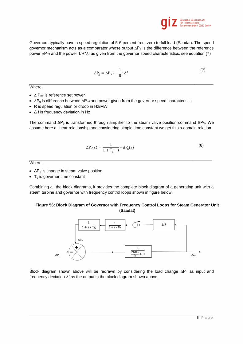
5 | P a g e
Governors typically have a speed regulation of 5-6 percent from zero to full load (Saadat). The speed
governor mechanism acts as a comparator whose output ∆Pg is the difference between the reference
power ∆Pref and the power 1/R*∆f as given from the governor speed characteristics, see equation (7)
ΔPg = ∆Pref −1
R∙ ∆f
(7)
Where,
∆ Pref is reference set power
∆Pg is difference between ∆Pref and power given from the governor speed characteristic
R is speed regulation or droop in Hz/MW
Δ f is frequency deviation in Hz
The command ΔPg is transformed through amplifier to the steam valve position command ΔPV. We
assume here a linear relationship and considering simple time constant we get this s-domain relation
∆Pv(s) =1
1 + Tg ∙ s∗ ∆Pg(s)
(8)
Where,
ΔPV is change in steam valve position
Tg is governor time constant
Combining all the block diagrams, it provides the complete block diagram of a generating unit with a
steam turbine and governor with frequency control loops shown in figure below.
Figure 56: Block Diagram of Governor with Frequency Control Loops for Steam Generator Unit
(Saadat)
Block diagram shown above will be redrawn by considering the load change ∆PL as input and
frequency deviation ∆f as the output in the block diagram shown above.
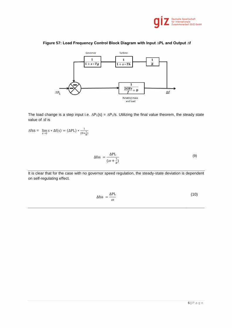
6 | P a g e
Figure 57: Load Frequency Control Block Diagram with Input ∆PL and Output ∆f
The load change is a step input i.e. ∆PL(s) = ∆PL/s. Utilizing the final value theorem, the steady state
value of ∆f is
∆fss = lims→0
s ∗ ∆f(s) = (∆PL) ∗1
(D+1
R)
∆fss =∆PL
( +1
𝑅) (9)
It is clear that for the case with no governor speed regulation, the steady-state deviation is dependent
on self-regulating effect.
∆fss =∆PL
(10)
7 | P a g e
Annexure 3
Reactive power markets of California
In both ISO and non-ISO markets, reactive power capability is paid on a cost-of-service basis to
transmission suppliers. Static sources of reactive power such as capacitors generally have their costs
rolled into transmission charges or into the regulated retail rate structure. As far as generators are
concerned, there are two general ways to compensate them for providing reactive power.
One way is the capacity payment option, in which the generator is paid in advance for the capability of
producing or consuming reactive power. The payment could be made through a bilateral contract or
through a generally applicable tariff provision. Once the generator is paid, it could be obligated to
produce or consume reactive power up to the limits of its commitment without further compensation
when instructed by the ISO. To ensure that the generator follows instructions in real time, the
generator could face penalties for failing to produce or consume when instructed. Currently, this is the
most common method for compensating reactive power providers.
The other way is the real-time price option, in which the generator is paid in real-time for the reactive
power that it actually produces or consumes. This pricing option falls under the general method of
nodal reactive power pricing. Under this option, the generator is paid only for what it produces or
consumes, but it pays no penalty for failing to produce when instructed. It is also possible to combine
some of the features of each of these options. For example, a generator might receive a capacity
payment in advance in exchange for the obligation to produce or consume reactive power within a
specified power factor range upon instruction by the ISO, but might also receive a spot price for
producing or consuming additional reactive power beyond the specified range. The capacity payment
under the capacity payment option can be based on cost based methods or the ISO could hold an
auction for reactive power capability and the winners of the auction would receive the applicable
market clearing price.
Under the real time option, the payment could be based on one of the following:
1. Pay nothing for reactive power produced within a specified power factor range. This option
may be most appealing when the generator has received a capacity payment in advance for
the capability to produce within the specified range.
2. Pay unit-specific opportunity costs due to reduced real power production.
3. Pay Market Clearing Prices determined through auction. MCPs are based on a spot market
auction for reactive power.
In the auction, all accepted bidders at a location could receive the same market-clearing price
based on the highest accepted bid. One issue for the auction is whether reactive power prices
are calculated directly or are derived from the implicit opportunity costs associated with real
power prices and the supplier’s real-power energy bids. Under the direct pricing approach,
reactive power sellers would submit price bids for supplying (or consuming) specific amounts
of reactive power and the reactive power price at any location and time would be the highest
accepted price bid. Under the derived approach, reactive power suppliers would submit price
bids for supplying real power as well as information indicating the trade-off between supplying
various amounts of real and reactive power. However, the supplier would not submit a
specific price bid for producing reactive power.
From the submitted information, the ISO would calculate the implicit opportunity cost (i.e., the
forgone real-power revenue associated with supplying or consuming reactive power) incurred

8 | P a g e
by each supplier. The price for reactive power in the auction would be calculated based on
these derived opportunity costs.
4. Pay a price based on a pricing formula announced in advance. This method is currently
used in the United Kingdom and India.
Reactive Power Management
ISO Responsibilities
The main responsibility for reactive power management in the California ISO Grid lies with the
California ISO. The ISO monitors loads and generators for operation at the appropriate voltage level,
verifies that each Participating Entity complies with voltage support requirements, and coordinates
adjustments to prevent offsetting or competing voltage support measures. The ISO also monitors the
interconnections with other Control Areas to confirm that the interconnected power system is operated
at the appropriate voltage level with acceptable MVAR exchange, and coordinates adjustments with
interconnected Control Areas as needed.
More specifically, the ISO coordinates the use of voltage support equipment among Participating
Transmission Owners (PTOs), Utility Distribution Companies (UDCs), Generators, and other
Control Areas in order to:
Ensure that Participating Entities maintain appropriate voltage schedules
Ensure that Participating UDCs maintain reactive power flow at grid interface points within an
appropriate power factor range, namely, 0.97 lag and 0.99 lead
Coordinate switching of voltage support equipment such as shunt capacitors and reactors
Ensure that Participating Generating units operate within an appropriate power factor range,
namely, 0.90 lag and 0.95 lead, unless otherwise specified in the relevant Participating
Generator Agreement (PGA)
Coordinate events and changes that impact the voltage support equipment availability,
reliability, or ability to operate within its applicable power factor range
Ensure that the grid provides the appropriate reactive power supply and reserves to the
interconnected power system
Coordinate and optimize voltage schedules and VAR flows between Control Areas for system
stability.
The California ISO does not operate a formal reactive power market. Reactive power and voltage
support is procured through long-term contracts with Reliability Must-Run (RMR) units. There are two
types of these contracts: Condition 1 and Condition 2.
Condition 1 RMR units may bid and participate in the market, but if they are needed for reliability, their
bids are mitigated to contractual cost-based rates, and they receive a portion of their fixed costs. Even
if Condition 1 RMR units do not bid in the Day-Ahead Market, the ISO may issue a RMR dispatch
notice for these units to run if they are needed for reliability.
Condition 2 RMR units may not bid in the market, but are dispatched by the ISO as needed for
reliability and they are paid all their fixed and operating costs.Aside from dispatching RMR Units,
nominal voltage support is automatically obtained from all Participating Generating units operating
within their applicable power factor range. Under exceptional conditions, the ISO may request
additional Voltage Support requiring operation outside of that power factor range.
The ISO conducts power flow studies periodically to determine future reliability and voltage/reactive
power requirements of the grid, reevaluating RMR contracts. Participating Entity Responsibilities
besides the ISO, Participating Entities are also responsible for reactive power management.

9 | P a g e
Participating Generators operate generating units within established protocols and procedures,
specifically normal MW/MVAR capacity profiles, at the applicable voltage schedule. Participating
Generators produce or consume reactive power when requested by the ISO, and notify the ISO of
coordinated voltage support equipment switching and of events and changes that impact the
MW/MVAR capacity, reliability, or ability to operate within the applicable power factor range.
Participating Loads/UDCs operate in accordance with Good Utility Practice within established
protocols and Operating Procedures, and adhere to specified voltage schedules. Participating
Loads/UDCs maintain reactive power flow at grid interface points within the applicable power factor
range, and notify the ISO of coordinated voltage support equipment switching and of events and
changes that impact the voltage support equipment availability, reliability, or ability to operate within
the applicable power factor range.
Participating Transmission Owners operate the system in accordance with Good Utility Practice and
in a manner that ensures safe and reliable operation. PTOs maintain appropriate voltage schedules,
and notify the ISO of coordinated voltage support equipment switching and of events and changes
that impact the voltage support equipment availability, or reliability.

10 | P a g e
Voltage Support Remuneration
Due to its locational effect and use, reactive power and voltage support is a reliability service that
cannot be procured through a market via a competitive auction as other ancillary services because of
market power concerns. Voltage support is mainly procured through long-term contracts with RMR
units.
Remuneration for voltage support is thus subject to the specific contractual arrangements. There is no
remuneration for nominal voltage support from Participating Generating units while they operate
within their applicable power factor range. This is because supply or consumption of reactive power
within that range does not have an appreciable impact on the active power generation capability, thus
it does not impede full participation in the energy market or the fulfillment of any contractual energy
agreements or financial commitments such as the Day-Ahead schedule. However, if the ISO instructs
the unit to provide additional voltage support by operating outside of the applicable power factor
range, the additional reactive power supply or consumption usually comes at some expense of active
power generation and thus may result in some lost opportunity cost. In this case, the additional
voltage support is remunerated the lost opportunity cost (LOC), which is calculated as follows: (Dr
Alex D Papalexopoulos, 2012)
LMP
is the Locational Marginal Price at the unit location
p is the unit operating level
c(p) is the unit energy bid as a function of its operating
level
b is the highest operating level of the unit’s energy
bid
a is the dispatch operating level required for
additional Voltage Support
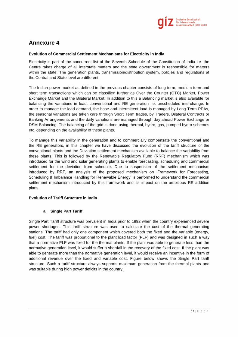
11 | P a g e
Annexure 4
Evolution of Commercial Settlement Mechanisms for Electricity in India
Electricity is part of the concurrent list of the Seventh Schedule of the Constitution of India i.e. the
Centre takes charge of all interstate matters and the state government is responsible for matters
within the state. The generation plants, transmission/distribution system, policies and regulations at
the Central and State level are different.
The Indian power market as defined in the previous chapter consists of long term, medium term and
short term transactions which can be classified further as Over the Counter (OTC) Market, Power
Exchange Market and the Bilateral Market. In addition to this a Balancing market is also available for
balancing the variations in load, conventional and RE generation i.e. unscheduled interchange. In
order to manage the load demand, the base and intermittent load is managed by Long Term PPAs,
the seasonal variations are taken care through Short Term trades, by Traders, Bilateral Contracts or
Banking Arrangements and the daily variations are managed through day ahead Power Exchange or
DSM Balancing. The balancing of the grid is done using thermal, hydro, gas, pumped hydro schemes
etc. depending on the availability of these plants.
To manage this variability in the generation and to commercially compensate the conventional and
the RE generators, in this chapter we have discussed the evolution of the tariff structure of the
conventional plants and the Deviation settlement mechanism available to balance the variability from
these plants. This is followed by the Renewable Regulatory Fund (RRF) mechanism which was
introduced for the wind and solar generating plants to enable forecasting, scheduling and commercial
settlement for the deviation from schedule. Due to suspension of the settlement mechanism
introduced by RRF, an analysis of the proposed mechanism on ‘Framework for Forecasting,
Scheduling & Imbalance Handling for Renewable Energy’ is performed to understand the commercial
settlement mechanism introduced by this framework and its impact on the ambitious RE addition
plans.
Evolution of Tariff Structure in India
a. Single Part Tariff
Single Part Tariff structure was prevalent in India prior to 1992 when the country experienced severe
power shortages. This tariff structure was used to calculate the cost of the thermal generating
stations. The tariff had only one component which covered both the fixed and the variable (energy,
fuel) cost. The tariff was proportional to the plant load factor (PLF) and was designed in such a way
that a normative PLF was fixed for the thermal plants. If the plant was able to generate less than the
normative generation level, it would suffer a shortfall in the recovery of the fixed cost. If the plant was
able to generate more than the normative generation level, it would receive an incentive in the form of
additional revenue over the fixed and variable cost. Figure below shows the Single Part tariff
structure. Such a tariff structure always supports maximum generation from the thermal plants and
was suitable during high power deficits in the country.
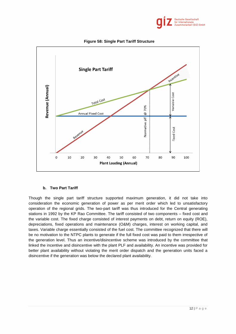
12 | P a g e
Figure 58: Single Part Tariff Structure
b. Two Part Tariff
Though the single part tariff structure supported maximum generation, it did not take into
consideration the economic generation of power as per merit order which led to unsatisfactory
operation of the regional grids. The two-part tariff was thus introduced for the Central generating
stations in 1992 by the KP Rao Committee. The tariff consisted of two components – fixed cost and
the variable cost. The fixed charge consisted of interest payments on debt, return on equity (ROE),
depreciations, fixed operations and maintenance (O&M) charges, interest on working capital, and
taxes. Variable charge essentially consisted of the fuel cost. The committee recognized that there will
be no motivation to the NTPC plants to generate if the full fixed cost was paid to them irrespective of
the generation level. Thus an incentive/disincentive scheme was introduced by the committee that
linked the incentive and disincentive with the plant PLF and availability. An incentive was provided for
better plant availability without violating the merit order dispatch and the generation units faced a
disincentive if the generation was below the declared plant availability.
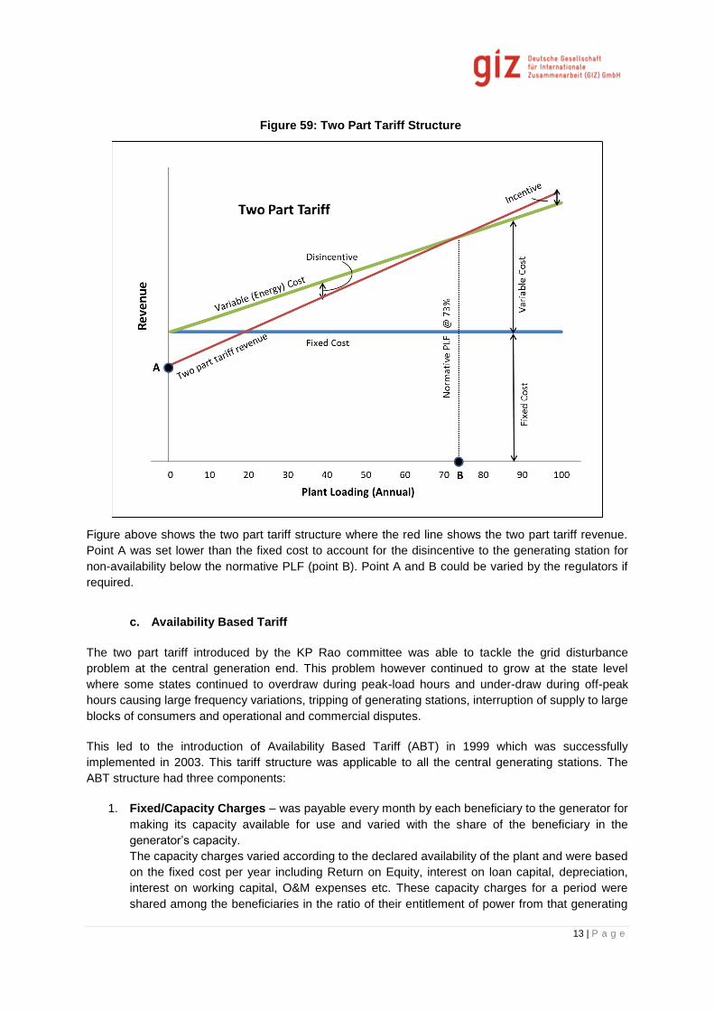
13 | P a g e
Figure 59: Two Part Tariff Structure
Figure above shows the two part tariff structure where the red line shows the two part tariff revenue.
Point A was set lower than the fixed cost to account for the disincentive to the generating station for
non-availability below the normative PLF (point B). Point A and B could be varied by the regulators if
required.
c. Availability Based Tariff
The two part tariff introduced by the KP Rao committee was able to tackle the grid disturbance
problem at the central generation end. This problem however continued to grow at the state level
where some states continued to overdraw during peak-load hours and under-draw during off-peak
hours causing large frequency variations, tripping of generating stations, interruption of supply to large
blocks of consumers and operational and commercial disputes.
This led to the introduction of Availability Based Tariff (ABT) in 1999 which was successfully
implemented in 2003. This tariff structure was applicable to all the central generating stations. The
ABT structure had three components:
1. Fixed/Capacity Charges – was payable every month by each beneficiary to the generator for
making its capacity available for use and varied with the share of the beneficiary in the
generator’s capacity.
The capacity charges varied according to the declared availability of the plant and were based
on the fixed cost per year including Return on Equity, interest on loan capital, depreciation,
interest on working capital, O&M expenses etc. These capacity charges for a period were
shared among the beneficiaries in the ratio of their entitlement of power from that generating
14 | P a g e
station. Even if the beneficiary does not need the supply, he has to bear the fixed charges. He
can however, sell the capacity entitlement to others.
2. Energy Charges – consisted of the variable or the fuel charges including the cost of
secondary fuel oil. These were charged only to the extent of the scheduled drawl by the
beneficiary.
3. Unscheduled Interchange Charge (UI Charge) – This was the new component added to the
tariff structure that accounted for incentives and disincentives for the generators on account of
variation from their schedule as per the system frequency at that point of time. This
component was introduced to enforce grid discipline among the sellers and buyers connected
to the grid.
Figure 60: Components of ABT
The Unscheduled Interchange Regulations were introduced in 2009 and the charges for Unscheduled
Interchange for all the time-blocks when grid frequency was between 50.3 Hz and 49.2 Hz were
payable for over-drawl by the beneficiary and under-injection by the generating station and receivable
for under-drawl by the beneficiary and over-injection by the generating station. These charges were
worked out on the average frequency of the 15 min time-block. The frequency range was further
reduced to 50.2 Hz to 49.5 Hz in 2012.
The regulation also introduced a limit on the over-drawl of electricity by any beneficiary not to exceed
12% of its scheduled drawl or 150 MW (whichever is lower) when the grid frequency was below 49.5
Hz, and 3% on a daily aggregate basis. Similarly, during the same situation with grid frequency below
49.8 Hz, no generator was allowed to under-inject more than 12% of its scheduled injection.
The UI mechanism enabled the beneficiaries to have proper schedules which allowed them to draw
power up to the specified limits at normal rates of the respective power plants. In case of over-drawl
during low grid frequency, they had to pay the UI charge which discouraged them from over-drawing
further. This payment then was passed to the beneficiaries who received less energy than their
schedule which acted as an incentive/compensation for them.
Deviation Settlement Mechanism
Though the ABT mechanism was able to introduce some grid discipline with the introduction of UI
charges, more changes were required to be introduced in the regulation to reduce the variations in the
grid frequency. Meanwhile, two consecutive major grid failures were experienced on consecutive days
on 30th and 31st July 2012. These incidents made it evident that other than the grid frequency,
parameters like transfer capability of transmission lines, voltage, etc., are equally important and need
Capacity Charges
Based on Declared Capacity
For recovery of Annual Fixed
Costs
Energy Charges
Based on Scheduled Generation
For Recovery of Primary Fuel
Costs
UI Charges
As per Frequency
Linked Rate
For Deviation from the Schedule
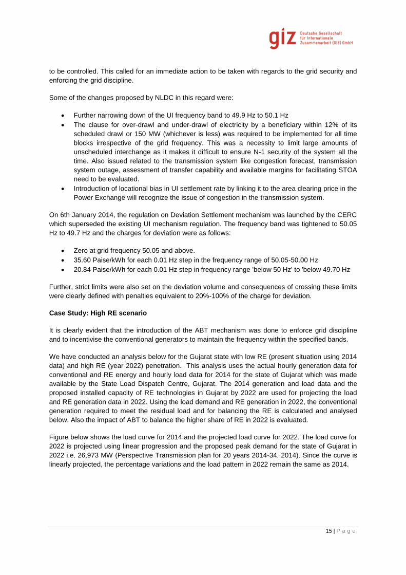
15 | P a g e
to be controlled. This called for an immediate action to be taken with regards to the grid security and
enforcing the grid discipline.
Some of the changes proposed by NLDC in this regard were:
Further narrowing down of the UI frequency band to 49.9 Hz to 50.1 Hz
The clause for over-drawl and under-drawl of electricity by a beneficiary within 12% of its
scheduled drawl or 150 MW (whichever is less) was required to be implemented for all time
blocks irrespective of the grid frequency. This was a necessity to limit large amounts of
unscheduled interchange as it makes it difficult to ensure N-1 security of the system all the
time. Also issued related to the transmission system like congestion forecast, transmission
system outage, assessment of transfer capability and available margins for facilitating STOA
need to be evaluated.
Introduction of locational bias in UI settlement rate by linking it to the area clearing price in the
Power Exchange will recognize the issue of congestion in the transmission system.
On 6th January 2014, the regulation on Deviation Settlement mechanism was launched by the CERC
which superseded the existing UI mechanism regulation. The frequency band was tightened to 50.05
Hz to 49.7 Hz and the charges for deviation were as follows:
Zero at grid frequency 50.05 and above.
35.60 Paise/kWh for each 0.01 Hz step in the frequency range of 50.05-50.00 Hz
20.84 Paise/kWh for each 0.01 Hz step in frequency range 'below 50 Hz' to 'below 49.70 Hz
Further, strict limits were also set on the deviation volume and consequences of crossing these limits
were clearly defined with penalties equivalent to 20%-100% of the charge for deviation.
Case Study: High RE scenario
It is clearly evident that the introduction of the ABT mechanism was done to enforce grid discipline
and to incentivise the conventional generators to maintain the frequency within the specified bands.
We have conducted an analysis below for the Gujarat state with low RE (present situation using 2014
data) and high RE (year 2022) penetration. This analysis uses the actual hourly generation data for
conventional and RE energy and hourly load data for 2014 for the state of Gujarat which was made
available by the State Load Dispatch Centre, Gujarat. The 2014 generation and load data and the
proposed installed capacity of RE technologies in Gujarat by 2022 are used for projecting the load
and RE generation data in 2022. Using the load demand and RE generation in 2022, the conventional
generation required to meet the residual load and for balancing the RE is calculated and analysed
below. Also the impact of ABT to balance the higher share of RE in 2022 is evaluated.
Figure below shows the load curve for 2014 and the projected load curve for 2022. The load curve for
2022 is projected using linear progression and the proposed peak demand for the state of Gujarat in
2022 i.e. 26,973 MW (Perspective Transmission plan for 20 years 2014-34, 2014). Since the curve is
linearly projected, the percentage variations and the load pattern in 2022 remain the same as 2014.

16 | P a g e
Figure 61: Gujarat Load Demand - 2014 and 2022
Similarly, the solar generation data for 2014, the installed capacity in 2014 and the expected solar
installed capacity in Gujarat by 2022 are used for linearly extrapolating the solar generation for 2022.
It is assumed that the solar insolation and the solar plant PLF remains the same in both the years. It is
also assumed that all the solar plants come up in the same locations as the existing ones. Figure
below shows the solar power generation curve for the month of July for 2014 and 2022. Only one
month data is shown in the graph to clearly understand the generation pattern from the solar plants.
The present solar installed capacity at the end of 2014 was 902.53 MW (CEA) and the proposed solar
capacity in Gujarat by 2022 is taken from MNRE which is 8020 MW. Due to such high growth in the
solar plants by 2022, high variations can be observed in the solar generation as shown in the graph
below.
Figure 62: Gujarat Solar Generation for July 2014 and July 2022
On similar terms, the wind generation is projected for the year 2022. Figure below shows the wind
power generation curve for the month of July for 2014 and 2022. The present installed capacity of
wind power at the end of 2014 was 3477.85 MW (CEA) and the proposed wind capacity in Gujarat in
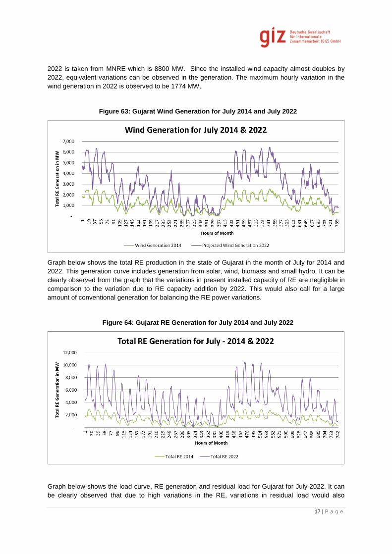
17 | P a g e
2022 is taken from MNRE which is 8800 MW. Since the installed wind capacity almost doubles by
2022, equivalent variations can be observed in the generation. The maximum hourly variation in the
wind generation in 2022 is observed to be 1774 MW.
Figure 63: Gujarat Wind Generation for July 2014 and July 2022
Graph below shows the total RE production in the state of Gujarat in the month of July for 2014 and
2022. This generation curve includes generation from solar, wind, biomass and small hydro. It can be
clearly observed from the graph that the variations in present installed capacity of RE are negligible in
comparison to the variation due to RE capacity addition by 2022. This would also call for a large
amount of conventional generation for balancing the RE power variations.
Figure 64: Gujarat RE Generation for July 2014 and July 2022
Graph below shows the load curve, RE generation and residual load for Gujarat for July 2022. It can
be clearly observed that due to high variations in the RE, variations in residual load would also

18 | P a g e
increase. As per the analysis, hourly variations of the order of 2900 MW will be observed in the state
in 2022 for the residual load i.e. the conventional generators need to be ramped up/ramped down to
cater to a variation of approx. 2900 MW. In addition to this, if we add the deviation of RE from the
schedule due to inaccurate forecasting, it might lead to a very difficult balancing situation for the state.
This would this call for the need of ancillary services to be introduced to cater to such variations.
Figure 65: Gujarat Load Demand v/s RE Generation & Residual Load for July 2022
Further, using the load and RE generation projections for 2022, we can calculate the amount of
conventional generation required for meeting the load demand and for balancing the RE power. The
installed capacity of conventional plants in Gujarat (including central generation allocation) in 2014
was 18307.37 MW. From the 2014 SCADA data available from Gujarat SLDC, it was found that the
average plant load factor for the conventional plants in the year 2014 was 55%. However, it increases
for the year 2022 to an average value of 71% as the load demand in the state will increase to 26,973
MW in 2022 (CEA data) against the 14,005 MW load in 2014..
Graph below shows the steady state frequency deviation when different shares of RE are added to
the grid (considering no speed regulation).

19 | P a g e
Figure 66: Frequency Deviation for Different Shares of RE
Figure above shows that the steady state frequency deviation would increase almost in a linear
fashion as the schedule deviation is increased. As the share of RE in the system increases, there is
drastic increment in the steady state frequency deviation. This is because the absolute value of the
potential deviation increases due to the uncertainty of predicting the RE through day ahead
forecasting. If the uncertainty in the system from RE increases, it is very difficult for the operator to
balance the load and generation.
The ABT mechanism incentivises/dis-incentivises the conventional generators as per their deviation
from schedule with the sole aim of maintaining the grid frequency at 50Hz. It can be clearly implied
from the above analysis that the ABT mechanism with the Deviation Settlement Mechanism would be
required to manage the grid frequency and stability when large amount of RE penetrates the system.
This is because along with the deviations from conventional generators, the variations in load also
need to be balanced by the conventional plants. For balancing the forecast errors of renewables, a
systematic change to fast acting reserve markets (with higher ramp up/down rates) would be a better
option. Another important step in the same direction would be to implement intra-state ABT as most of
the RE generators today are connected to the intra-state transmission system.
The DSM however is applicable only to the conventional generation plants. To enable scheduling of
wind and solar power and the commercial settlement attached to it, the Renewable Regulatory Fund
(RRF) mechanism was introduced by CERC.
Renewable Regulatory Fund Mechanism
To reduce the impact of variations from the RE sources, forecasting and scheduling the RE
generation was needed. In this regard, the draft Indian Electricity Grid Code (second amendment)
was issued containing the scheduling provisions for RE generation in February 2010. The draft IEGC
was soon notified in May 2010 that included the scheduling of wind and solar generation to start from
1st January 2011. This was later postponed to 1st January 2012 so that the states can be prepared to
adapt to the mechanism. In December 2011, CERC initiated the Suo Motu proceedings in the matter
of implementation of the RE Regulatory Fund (RRF) mechanism as most of SLDCs were not
prepared to adapt to the new mechanism. A Task Force was constituted to provide solution to this
issue. After taking into account Task Force Report, CERC notified an Order dated January 16, 2013.

20 | P a g e
The salient features of the Order were as given below:
Point of scheduling/Scheduling Entity could be any of the generators or any other mutually
agreed agency.
Pooling stations commissioned after May 3, 2010 will only be selected.
Payment Mechanism would follow actual generation based accounting.
Sharing of financial implication among generators to be mutually agreed between Scheduling
entity and generators. In case of disagreement implications to be shared in the ratio of actual
generation on a weekly basis.
STU/DISCOMs were directed to install ABT meters at all pooling stations and in case not
installed, CTU shall install the same at the cost of STU/DISCOM.
The RRF guidelines were issued on July 9, 2013 which directed that the scheduling of RE power
would start from July 15, 2013. The main aim of the regulation was to enable forecasting and
scheduling of the RE power and to introduce a commercial settlement mechanism to penalise the
wind generators if they deviated from the schedule beyond a limit. Solar generators were exempted
from the penalty to give more time to the technology to mature. The key points covered under this
regulation were:
For Wind Energy Generators:
All wind generators connected to the pooling stations of 33 kV and above with collective
capacity of 10MW and above are obligate under this mechanism.
The wind generators shall be responsible for forecasting their generation at the pooling
station level up to accuracy of 70%. Therefore, if the actual generation is beyond ± 30% of the
schedule, UI charges would be applicable to the wind generator. For actual generation within
± 30% of the schedule, no UI would be payable/receivable by Generator.
UI charges for within this variation, i.e. within ± 30% would be applicable to the host state.
However, the implication of these UI charges shall be shared among all the States/UTs of the
country/DVC in the ratio of their peak demand met in the previous month based on the data
published by CEA, in the form of a regulatory charge known as the RE Regulatory Charge
operated through the RE Regulatory Fund (RRF).
A maximum generation of 150% of the schedule only, would be allowed in a time block, for
injection by wind, from the grid security point of view. For any generation above 150% of
schedule, if grid security is not affected by the generation above 150%, the only charge
payable to the wind energy generator would be the UI charge applicable corresponding to 50-
50.02 HZ.
In the case of intra-State sale of wind energy, the transactions would be be-tween the wind
generator and the host State at the contracted rate for actual generation. The implication due
to deviations of actual generation within ± 30% of the scheduled generation would be settled
through the RRF. The implication due to deviations outside ± 30% would be settled directly
between the host State and the Wind Farm in accordance with the energy accounts issued by
the RPC.
In the case of inter-State sale of wind energy, the transactions would be be-tween the wind
generator and the purchasing State at the contracted rate for actual generation up to 150% of
the scheduled generation. The difference of actual generation from the schedule for the
purchasing State would be settled at the UI rate of the Region of the purchasing State through
the RRF. The implication due to deviations of actual generation within ± 30% of the scheduled
generation would be settled with the host State through the RRF. The deviations outside ±
30% would be settled directly between the host State and the Wind Farm in accordance with
the energy accounts issued by the RPC.

21 | P a g e
For Solar Generators:
Applicable to Pooling Stations of Solar generating plants with capacity of 5 MW and above
connected at connection point of 33 kV level and above.
The schedule of solar generation shall be given by the generator based on availability of the
generator, weather forecasting, solar insolation, season and normal solar generation curve
and shall be vetted by the RLDC in which the generator is located and incorporated in the
inter-state schedule. If RLDC is of the opinion that the schedule is not realistic, it may ask the
solar generator to modify the schedule.
In case of solar generation no UI shall be payable/receivable by Generator.
In the case of intra-State sale of solar energy, the host State would pay the solar generator at
the contracted rate for actual generation.
In the case of inter-State sale of solar energy, the purchasing State would pay the solar
generator at the contracted rate for actual generation. The implication of UI charges due to
the deviation for purchasing State and host State would be settled through the RRF.
To enable RRF mechanism, the RE developers had to forecast and schedule their power which would
require installation of special energy meters (which can provide data in 15 minute time-blocks),
developing a method/ tool for forecasting, scheduling of RE power and continuous monitoring of the
weather conditions to alter the schedule if required (maximum of 8 revisions for each 3 hour time slot).
This instrument would have led to better grid discipline and higher system security as it aimed at
reducing the effect of variations from RE generators on the grid frequency. Also, keeping in mind the
ambitious RE addition plans of 175GW by 2022 defined by the Government of India, the RRF
mechanism would have played a very vital role in maintaining a higher system security.
The regulation however received a lot of criticism from the wind developers due to the following
reasons:
Unavailability of any robust forecasting mechanism to accurately schedule power within the
prescribed range.
Large variations of wind power from the forecast.
Wind developers were unable to meet the forecasting accuracy most of the times.
Further, the CERC order on RRF was challenged in three high courts of the country by three different
organisations. Indian wind power association (IWPA) has filed an injunction against the regulation in
Delhi High Court, Wind Independent Power Producers' Association (WIPPA) in Madras High Court
and Gujarat Mineral Development Corporation (GMDC) in Ahmedabad High Court. Wind power
producers challenged the regulation on grounds of both feasibility and legality. Some power
producers also questioned the preparedness of the national grid to handle modern data collection
technology.
After receiving negative feedback from the wind developers regarding implementation of the RRF
mechanism, on January 7, 2014 the CERC suspended the commercial mechanism of RRF keeping
the clause for scheduling of wind generation intact as per the provisions of the Grid Code and RRF
procedure.
However, the ambitious plans of the Indian government to add significant amount of RE power in the
grid called for a revised regulation. Recently, on March 31, 2015 CERC proposed the draft framework
for Forecasting, Scheduling & Imbalance Handling for RE Generating Stations based on wind and

22 | P a g e
solar at Inter-State Level including draft amendments to the IECG, DSM and REC regulations which is
discussed in detail in the next section.
Proposed Framework for Forecasting, Scheduling & Imbalance Handling for Renewable
Energy
Some of the key features of the proposed framework are:
Applicable to all wind/solar energy generators who are designated as regional entities and
whose scheduling at the inter-state level is done by the RLDCs.
Centralized and De-centralized Forecasting: To be done by the wind/solar generator and the
concerned RLDC.
Both wind and solar energy generation are brought under the requirement of forecasting and
scheduling and are subjected to commercial impact on account of deviation from schedule.
16 revisions for each 1.5 hours’ time slot for both Solar and Wind generators.
Deviation charges delinked from frequency and the desired operating band of ± 12% is set for
the wind and solar energy generators.
One of the important points to be noted is that the proposed framework is applicable to individual
wind/solar generators with an operating band of ± 12% as opposed to the earlier RRF mechanism
which was applicable for a larger control area (aggregate level of a pooling station) with an operating
band of ±30% but was still questioned and suspended later due to opposition from the wind
developers.
Table below gives the new proposed deviation settlement for RE generators as per the proposed
framework.
Table 19: Proposed Deviation Settlement for RE Generators
Ranges Below 88%
of Schedule
In between
88% - 100%
of Schedule
In between
100% - 112%
of Schedule
Beyond 112%
of Schedule
Proposed
Settlement for the
RE Energy under
DSM Pool Account
(Scheduled
power @ PPA) –
(Rs.4/kWh of
under
generation
below 88% to
DSM pool
Account)
Generators have
to procure REC
to the extent of
energy under
generated
(Scheduled
power @ PPA) –
(Rs.3/kWh of
under
generation DSM
pool Account)
Generators have
to procure REC
to the extent of
energy under
generated
(Scheduled
power @ PPA) +
(Rs.4/kWh of
over generation
from DSM pool
Account)
Generators will
be provided with
REC to the
extent of energy
over generated
Generator will
not receive any
amount for
excess
generation
beyond 112% of
Schedule
Generators will
be provided with
REC to the
extent of energy
over generated
(Settlement price of Rs. 3/kWh and Rs. 4/kWh are indicative and shall be revised by CERC regularly)
23 | P a g e
Case Study
A comparison of the commercial settlement using the suspended RRF mechanism and the proposed
DSM amendment was conducted for a wind farm and a solar plant connected at the inter-state level
at different percentage deviation and different frequency.
The analysis was performed considering the following key assumptions:
Tariff for wind generator = Rs. 5/kWh
Tariff for solar generator = Rs. 7/kWh
Floor Price of solar REC = Rs. 3.5/kWh
Floor Price of non-solar REC = Rs. 1.5/kWh
Reference rate for wind for NEW grid = Rs. 4/kWh (For calculation of deviation charge
using RRF mechanism. Source:
https://www.sldcguj.com/RRF/RRF_Presentation%20WF%20Meet%2013.04.13.pdf)
UI Rates for the RRF calculation are taken as per the Second Amendment of
Unscheduled Interchange Regulation.
In 2013, it was suggested by CERC to treat the reference rate of wind as Rs. 4/unit for NEW Grid and
Rs. 5/unit for Southern grid. This rate was fixed based on UI rate of frequency of the previous financial
year. Since the NEW grid and the southern grid were connected on 31st December 2013 and the RRF
mechanism was suspended on 7th January 2014, a new reference rate for the combined grid was not
announced. For this calculation, we are taking the reference rate as Rs. 4/unit which is same as the
NEW grid.
Following formulae were used to calculate the charges due to RRF:
Payment received by RE Generator due to actual generation (in Rs.) = Actual generation in
MW x 1000 x Tariff in Rs./kWh [upto a maximum of 150%]
RRF charges [paid (-ve) / received (+ve) by the generator] in Rs.
For deviation between ±30% For deviation between +30%
to +50% and -30% to -50% For deviation beyond ±50%
Zero
Deviation in MW between 30-
50% x 1000 x (Reference rate –
UI charge at the said frequency)
Deviation in MW between 30-
50% x 1000 x (Reference rate –
UI charge at the said frequency)
+ Deviation in MW beyond 50%
x 1000 x (Deviation charge at
frequency 50-50.02 Hz)
Net payment received by RE generator (Rs.) = Payment received by RE Generator due to
actual generation + RRF charges
The UI charges as per the Second Amendment of Unscheduled Interchange Regulations are taken as
follows:
At 50.15 Hz = Rs. 0.495/kWh
At 50.04 Hz = Rs. 1.32/kWh
At 50.00 Hz = Rs. 1.65/kWh
At 49.80 Hz = Rs. 4.5/kWh
At 49.70 Hz = Rs. 5.9063/kWh

24 | P a g e
The detailed calculations can be found in Annexure 1. Table below gives the calculation of deviation
settlement for a wind farm at grid frequency of 50.15 Hz using the RRF mechanism and the proposed
DSM regulation. Similar analyses were also done at other frequencies like 50.04, 50, 49.8 and 49.7
Hz.
Table 20: Analysis of RRF and Proposed DSM for RE Generators
Inter-State Wind
Hz
Schedul
ed
generati
on (MW)
Actual
Generatio
n (MW)
%
deviatio
n
Charges due to RRF (in Rs.) Charges due to Proposed DSM (in Rs.)
Payment
received
by RE
Generato
r due to
actual
generatio
n
RRF
charges
paid (-
ve) /
received
(+ve) by
the
generat
or
Net
payment
received
by RE
generat
or
RE
Generator
gets due
to
schedule
d
generatio
n
RE
generat
or pays
to (-ve)
or gets
from
(+ve)
the DSM
Pool
RE
generat
or pays
(-ve) or
gets
(+ve) for
RECs
Net
payment
received
by RE
generato
r
50.1
5
100 160 60 750000 -53600 696400 500000 48000 90000 638000
100 140 40 700000 -35050 664950 500000 48000 60000 608000
100 120 20 600000 0 600000 500000 48000 30000 578000
100 110 10 550000 0 550000 500000 40000 15000 555000
100 90 -10 450000 0 450000 500000 -30000 -15000 455000
100 80 -20 400000 0 400000 500000 -68000 -30000 402000
100 60 -40 300000 35050 335050 500000 -148000 -60000 292000
100 40 -60 200000 105150 305150 500000 -228000 -90000 182000
The % deviation from the schedule for each frequency is taken from +60% to -60% as given in the
table above. This was intentionally done to evaluate the commercial impact of the two regulations in
the deviation bands of upto12%, 12-30% and beyond ± 30%. The following can be observed from the
above calculations:
The net payment received by the RE generator was higher due to RRF regulation as
compared to the proposed DSM regulation for all % deviation except the +10%, -10% and -
20% deviation levels. This is mainly because the allowable deviation band is reduced to ±12%
as compared to ±30% in RRF mechanism. This implies the RE generator now pays the
deviation charges for ± 12-30% deviation from schedule.
When the RE generation is within 88-100% of its schedule, the RE generator gets paid for the
scheduled power i.e. 100 MW (@ Rs. 5/unit) but needs to pay Rs. 3/unit to the DSM pool and
Rs. 1.5/unit to purchase REC for the shortfall in the generation. Thus, the RE generator still
gains Rs. 0.5/unit for the energy it never generated. This could be a potential area for gaming
by the RE generators. Though it is clear that this is intentionally introduced by CERC to
incentivise the RE generators, suitable steps need to be taken to ensure that gaming is not
taking place.

25 | P a g e
Table 21: Per Unit Charges for a Wind Generator as per Proposed DSM Mechanism
Per unit charges due to deviation for a Wind Generator
Deviation from Schedule Below
88%
Between
88% -
100%
Between
100% -
112%
Beyond
112%
Payment received by RE generator due to
Scheduled Power
5 5 0 0
Incentive/Disincentive due to deviation (DSM
Pool)
-4 -3 4 0
Incentive/Disincentive due to purchase of RECs -1.5 -1.5 1.5 1.5
Total Incentive/Disincentive per unit of
unscheduled generation
-0.5 0.5 5.5 1.5
It can also be observed that both the approaches systematically reward over-generation. The
RE generator gets paid higher when it generates beyond the +12% (i.e. at 20-60% deviation)
as compared to the compensation received within the ± 12% band.
It can be observed from the table above that the RE generator is incentivised when it
generates between the 100-112% (generator receives Rs. 5.5/unit) band. However, there is
no incentive provided to the RE generator when it meets its schedule i.e. 100% (generator
receives Rs. 5/unit). This needs to be addressed in the proposed DSM mechanism otherwise
the generators would not be encouraged to forecast and meet the schedule accurately. Also it
is not clear if the 100% generation falls in the 88-100% band or in 100-112% band.
When the grid frequency is greater than 50 Hz, it will call for the RE plants to reduce their
generation to contribute in maintaining the grid frequency. However, since the RE generator is
dis-incentivised when its actual generation is less than its schedule, it will not be encouraged
to reduce its generation beyond 88%. This might be an unfavourable situation and in future
when large amounts of RE are integrated into the grid; maintaining the grid frequency within
the prescribed range might become more difficult.
Similarly, when the RE generators are producing more than 112% of their schedule, they are
only provided with RECs for the excess generation. This might be an adequate incentive
when the grid frequency is above 50 Hz. However, when the grid frequency drops below 50
Hz, the RE generators need to be incentivised more to encourage them to improve the grid
frequency.
Table below shows the comparison of the net payment received from RRF and proposed DSM
mechanism when the schedule is within ± 12% which is as proposed by the DSM mechanism.

26 | P a g e
Table 22: Analysis of RRF and Proposed DSM for RE Generators for deviation within ±12%
Inter-State Wind
Hz
Schedul
ed
generati
on (MW)
Actual
Generatio
n (MW)
%
deviatio
n
Charges due to RRF (in Rs.) Charges due to Proposed DSM (in Rs.)
Payment
received
by RE
Generato
r due to
actual
generatio
n
RRF
charges
paid (-)/
received
(+) by
the
generat
or
Net
payment
received
by RE
generat
or
RE
Generator
gets due
to
schedule
d
generatio
n
RE
generat
or pays
to or
gets
from
DSM
Pool
RE
generat
or pays
or gets
for
RECs
Net
payment
received
by RE
generato
r
50.1
5
100 110 10 550000 0 550000 500000 40000 15000 555000
100 90 -10 450000 0 450000 500000 -30000 -15000 455000
50.0
4
100 110 10 550000 0 550000 500000 40000 15000 555000
100 90 -10 450000 0 450000 500000 -30000 -15000 455000
50 100 110 10 550000 0 550000 500000 40000 15000 555000
100 90 -10 450000 0 450000 500000 -30000 -15000 455000
49.8 100 110 10 550000 0 550000 500000 40000 15000 555000
100 90 -10 450000 0 450000 500000 -30000 -15000 455000
49.7 100 110 10 550000 0 550000 500000 40000 15000 555000
100 90 -10 450000 0 450000 500000 -30000 -15000 455000
After conducting the analysis, it was clearly observed that if the payment received by the RE
generator is calculated as per the proposed DSM structure, the generator is incentivised more if it
stays within the prescribed band of ± 12% of its schedule. This payment is also more than what the
generator would have received under the older RRF regulation. For all other deviation beyond ±12%,
the payment received by the proposed DSM is lower than what the generator would have received
from RRF mechanism. Thus, though the new mechanism has delinked the RE generation from
frequency, it is enforcing the desired operating band of ±12% for the RE generators.
As given in the present DSM regulation for conventional plants, handling of the infirm power injected
into the grid by the new RE generators before the commissioning date needs to be addressed in the
proposed regulation.
As per the proposed mechanism, if the RE generators are providing the forecast for their generation,
they would bear the cost of Forecasting, telemetry, SCADA, Communication facilities etc. This would
have an impact on the capital cost of the RE plants and thus the additional cost of forecasting
services needs to be included in the generic tariff which is determined by the Commission.
As per the proposed mechanism, the wind/solar generator needs to purchase RECs from the
exchange and give it to the buyer for any shortfall of energy produced and in case of excess
generation, the generator gets RECs equivalent to the extra energy produced. Since a lot of RECs
are already available with the wind/solar generators, the RE generator should be allowed to trade the
existing RECs (provided their validity is not expired) and the RECs received due to excess
generation. This would help the RE generators to off-set/transfer the RECs issued to them. In case of
shortage of RECs, the RE generators can procure them from the power exchange.

27 | P a g e
Due to the infirm nature of the solar and wind resource, the RE generators are bound to over/under
inject into the grid. RLDC can be given the responsibility to compile the energy account for each
generator on a monthly/quarterly basis. Further, the timeline for the issuance/purchase of RECs by
the wind and solar generators needs to be specified in the framework.
Error Analysis of forecasted GHI series in Rajasthan
The case considered here, discusses day-ahead solar resource forecasting techniques employed for
Rajasthan. Day-ahead forecasting or NWP model based solar resource forecasting started with
obtainment of NWP model output data from European Center for Medium Range Weather Forecast
(ECMWF) (Tripathy, 2015).
NWP models are mathematical equations describing the physical and dynamic processes in the
atmosphere. These equations are numerically solved on a 3D grid, taking measured atmospheric
conditions as initial input and the output from NWP model is the forecasted weather parameter. In our
case, the forecasted weather parameter was Surface Solar Radiation Downwards or SSRD. SSRD is
the shortwave solar radiation values with temporal resolution of 3 hours accumulated over the
temporal horizon of 72 hours. Now, these NWP model output solar radiations values were converted
to NWP model GHI by isolating irradiation value for each time step and normalizing with respect to the
time interval as the final requirement is forecasted GHI values. Then, the temporal resolution of NWP
model output GHI was interpolated down to 1 hour resolution using Inverse Distance Weighted (IDW)
method. The NWP GHI values of 1 hour resolution were further post processed using multiple
regression technique to account for local geographical conditions. The techniques mentioned before
were repeated for both local area forecast and wide area forecast.
The Forecasted GHI series obtained after statistical post processing were validated against irradiance
values measured at Solar Radiation Resource Assessment (SRRA) stations using statistical error
measures like root mean square error (RMSE), mean bias error (MBE) and standard deviation of error
(Stderr) defined by Management & Exploitation of Solar Resources (MESoR) committee.
As observed during this work, the error associated with single site forecast/local area forecast was
more compared to that of forecast with multiple sites. In wide-area forecasts, smoothing due to spatial
averaging lead to reduced degree of uncertainty. From grid operation, management & control point of
view, wider regional control area holds greater significance compared to that of a single generator.
Hence, it can be concluded that site-specific forecasting can be avoided and forecasting done at
SLDC level will be more apt.
Forecasted GHI series obtained, for single site/ local area analysis and multiple site/ wide area
analysis, have m\been validated against measured GHI values acquired from Solar Radiation
Resource
Assessment stations in Rajasthan. Statistics error measures defined by MESoR [Beyer et al, 2009]
have been estimated and are used to evaluate the accuracy of solar resource forecasting. The
following table shows relative error values evaluated for different techniques.

28 | P a g e
Figure 67 - Forecasted GHI series
As can be noticed, least relative error values are achieved for forecasted GHI series obtained after
statistical post processing. The following suggestions can be made from the study.
For spatial scale of forecast
o The error associated with single site forecast/local area forecast is more compared to that of
forecast with multiple sites. In wide-area forecasts, smoothing due to spatial averaging
reduces degree of uncertainty drastically. From grid operation, management & control point of
view, wider regional control area holds greater significance compared to that of a single
generator. Hence, it can be concluded that site-specific forecasting can be avoided and
forecasting done at regional level will be more apt.
For temporal resolution of forecast
o As per CERC, day-ahead scheduling (thus forecasting) is needed at a temporal resolution of
15 minutes. One hour resolution GHI, obtained can be further interpolated down to 15
minutes scale. Though the uncertainty level will not vary much under clear sky conditions, the
same may not be the case under cloudy conditions. It is also suggested to have an efficient
now-casting infrastructure along with day-ahead as, together they will be very accurate for
solar resource forecasting.
For forecast at a single generator/pooling station level
o Under the current scenario, it is not possible to differentiate a single generator from a pooling
station on the basis of spatial scale as both will be part of (2 X 2) grid as depicted in the
following figure for Rajasthan. Hence, forecasted GHI values evaluated for that spatially
averaged grid/ local area will be applicable to any solar generator or pooling station in that
area. But in future, it may be possible to evaluate forecast at a single generator level due to
simulation at even finer grid may be (1 km X 1 km) owing to greater computing power.

29 | P a g e
Figure 68 - IFS gridded map of Rajasthan
Recommendations and Comments on the draft regulation on the Proposed Framework for
Forecasting, Scheduling & Imbalance Handling for RE Energy
1. The proposed framework is applicable to individual wind/solar generators with an operating
band of ± 12% as opposed to the earlier RRF mechanism which was applicable for a larger
control area (aggregate level of a pooling station) with an operating band of ±30% but was
still questioned and suspended later due to opposition from the wind developers. As a
starting step, a higher operating band can be suggested for the RE generators which can
be then reduced over the years when the developers are able to achieve sufficient accuracy
in their forecasts.
2. Graph below clearly depicts the increase in the forecast accuracy when the forecast is done
at the regional level and not a single site forecast.

30 | P a g e
Figure 69: Change in Forecast Error for a Regional and Single Site Forecast
It is thus recommended that the RE forecast should be provided using an aggregator model
as being implemented in Tamil Nadu by IWPA. The accuracy requirements for the RE
generators should be set for the larger control area and not for single turbine level.
Also for single generators or small capacities, the forecast errors will be large with respect
to scheduled generation and would be difficult to be brought in the proposed range of
±12%.
3. As per the proposed mechanism, the number of revisions in the schedule has been revised
from 8 revisions for each 3 hour time slot for Wind generators to 16 revisions for each 1.5
hours’ time slot for both Solar and Wind generators. From the figure below it can be
observed that the prediction accuracy of a forecast increases when the forecast is done
closer to the time of generation.
This increase in the number of revisions in schedule will increase the potential for correcting
and adjusting the power forecasts. However, this cannot be done based on new available
meteorological forecast as these are typically provided twice a day. Also, a positive impact
on forecasting accuracy only can be achieved if measurement data from the operating wind
farms are available on-line and the forecast system makes use of this information.
4. The draft regulation has increased the number of revisions to the schedule submitted by RE
generators from 8 to 16. However, provisions need to be made to check the transmission
system availability and thus avoid transmission congestion before approving these
revisions.
5. From a technical point of view, even a 30% bandwidth has resulted already in a very high
number of cases outside of this range. Forecast errors of that size (and larger) are common
for single forecast events (one site). However, the relative r.m.s.e. of e.g. wind power
forecasts are calculated for a period of – at least – months and in so far represent a much
more appropriate way of forecast quality. For a medium-sized region this value then is (in
Europe) typically as low as 4%.
There is no obvious motivation for a specific value on the bandwidth of deviation – neither
30% nor 12%. The major impact of reducing the bandwidth is – of course – an increase in

31 | P a g e
the amount of the penalties. This goes along with a loss of revenues for the producer and –
in a worst case – could result in a drop of investments in RE power systems.
Figure 70: Accuracy of forecast for different Prediction Horizons
Renewable energy will have better predictability as we go near the dispatch time.
Therefore, a better forecast can be prepared if more number of revisions are available. It
is thus suggested to retain the increased number of revisions in the proposed
mechanism.
6. The proposed regulation is only applicable to wind and solar plants connected to the inter-
state network. Since the number of such plants is very low at present and most of the RE
plants are connected to the intra-state network, similar mechanism should also be
introduced for intra-state RE projects.
7. It is proposed in the framework that the charges for penalty/incentive would be a fixed
number which would be reviewed and updated by the commission from time to time.
However, since the PPA rate of different RE generators varies from each other, the
proposed settlement calculation may lead to higher penalties for plants with lower tariffs
and undue benefits for plants with higher tariffs. This is explained in the table below taking
the example of a wind plant:

32 | P a g e
Table 23: Impact of Proposed DSM Mechanism due to different PPA Rates
Deviation from Schedule Below
88%
Between
88% -
100%
Between
100% -
112%
Beyond
112%
Plant with lower PPA rate = Rs. 3.5/unit
Payment received by RE generator due to
Scheduled Power
3.5 3.5 0 0
Incentive/Disincentive due to deviation (DSM Pool) -4 -3 4 0
Incentive/Disincentive due to purchase of RECs -1.5 -1.5 1.5 1.5
Total Incentive/Disincentive per unit of
unscheduled generation
-2.0 -1.0 5.5 1.5
Plant with higher PPA rate = Rs. 6.0/unit
Payment received by RE generator due to
Scheduled Power
6 6 0 0
Incentive/Disincentive due to deviation (DSM Pool) -4 -3 4 0
Incentive/Disincentive due to purchase of RECs -1.5 -1.5 1.5 1.5
Total Incentive/Disincentive per unit of
unscheduled generation
0.5 1.5 5.5 1.5
It can be observed that plants with lower PPA rate are dis-incentivised in the 88-100%
deviation range and the plants with higher PPA rates benefitted even if their deviation is
below 88%. Thus for designing a fair compensation structure, the incentive/disincentive
received/paid to the DSM pool can be a percentage of the PPA rate.
8. The regulation involves a lot of payments between stakeholders without any physical
settlement of the imbalance. It would be better if the payments for imbalance reflect the
costs of imbalance settlement; however there is no mechanism introduced which assesses
these costs. The payments for over-drawl and under-drawl might not equal out and there
might be a gap to be funded i.e. if more payments towards generators are necessary than
generators paying into the fund, additional financing would be needed.
9. The proposed mechanism will lead to high payments in lean wind season also; when the
wind generation is very low but forecast error with respect to schedule will frequently be
high although the impact on the system is low as the absolute quantity of deviation in MW is
low. This can be seen in the figure below.

33 | P a g e
-150%
-100%
-50%
0%
50%
100%
0% 20% 40% 60% 80% 100%
De
viat
ion
of
real
ge
ne
rati
on
fro
m d
ay-a
he
ad
fore
cast
(%
)
Actual Generation % of Total Installed Capacity
Figure 71: Scatter plot linking forecast error to actual generation in % of total installed
capacity
Imprint
The findings and conclusions expressed in this document do not
Necessarily represent the views of the GIZ or BMZ.
The information provided is without warranty of any kind.
Published by
Deutsche Gesellschaft für
Internationale Zusammenarbeit (GIZ) GmbH
Indo – German Energy Programme – Green Energy Corridors
Registered offices: Bonn and Eschborn, Germany
B-5/2, Safdarjung Enclave
New Delhi 110 029 India
T: +91 11 49495353
I: www.giz.de
Authors Shuvendu Bose (Ernst and Young LLP)
Sudhanshu Gupta (Ernst and Young LLP)
Wolfram Heckmann (Fraunhofer IWES)
Editors
NS Saxena (Ex-Director PowerGrid Corporation)
New Delhi, October 2015
This project/programme’ assisted by the German Government,
is being carried out by ‘Ernst & Young LLP’ on behalf of the
Deutsche Gesellschaft für Internationale Zusammenarbeit
(GIZ) GmbH.