Embed Size (px)
Citation preview
1
Market Discipline in the Secondary Bond Market:
The Case of Systemically Important Banks
Elyas Elyasiani
Fox School of Business and Management
Temple University
Jason M. Keegan*
Supervision, Regulation, and Credit
The Federal Reserve Bank of Philadelphia
This Version:
January 17, 2017
JEL Classification: G01, G2, G21, G28
Keywords: Bank Risk; Financial Crisis; U.S. Bank Holding Companies; Risk Management;
Market Discipline
*The views expressed here are those of the authors and do not necessarily reflect those of the
Federal Reserve Bank of Philadelphia, the Board of Governors of the Federal Reserve System, or
the Federal Reserve System.

2
Abstract
We investigate the association between the yields on debt issued by U.S. Systemically Important
Banks (SIBs) and their idiosyncratic risk factors, macroeconomic factors, and bond features in
the secondary market. Although greater SIB risk-levels are expected to increase debt yields
(Evanoff and Wall, 2000), prevalence of government safety nets complicates the market
discipline mechanism, rendering the issue an empirical exercise. Our main objectives are
twofold. First, we study how bond-buyers reacted to elevation of SIB and macroeconomic risk
factors over the recent business cycle. Second, we investigate the degree to which the
proportions of the variance in yields explained by these two risk categories changed across the
phases of the cycle. Our data include over 8 million bond trades across 26 SIBs. We divide our
sample period into the pre-crisis (2003:Q1 to 2007:Q3), crisis (2007:Q4 to 2009:Q2), and post-
crisis (2009:Q3 to 2014:Q3) sub-periods to contrast the findings. We obtain several results. First,
bond-buyers do react to changes in the SIB risk factors (leverage, credit risk, inefficiency, lack of
profitability, illiquidity, and interest rate risk) by demanding higher yields. Second, bond
buyers’ responses to risk factors are sensitive to the phase of the business cycle. Third, the
proportion of variance in yields driven by SIB-specific and bond-specific risk factors increased
from 23% in the pre-crisis period to 47% and 73% during the crisis and post-crisis periods,
respectively. These findings indicate that the force of market discipline improved greatly during
the crisis and post-crisis periods, at the expense of the macroeconomic factors. The
strengthening of market discipline in the crisis and post-crisis periods, despite the
unprecendented regulatory intervention in the form of quantitative easing (QE), troubled asset
relief program (TARP), large bail outs and generally accomodative fiscal and monetary policies
adopted during these periods, demonstrates that regulatory intervention and market discipline can
work in tandem.
3
1. Introduction
We investigate how the yield-spreads1 on the debt issued by U.S. Systemically Important
Banks (SIBs) in the secondary market are associated with their idiosyncratic risk,
macroeconomic factors, and bond-specific features across the pre-crisis (2003:Q1 to 2007:Q3),
crisis (2007:Q4 to 2009:Q2), and post-crisis (2009:Q3 to 2014:Q3) phases of the recent business
cycle.2 We focus on the SIB population because, if mandatory debt issuance were to become a
part of the regulatory framework, as recommended e.g., by the joint report submitted to Congress
by the Board of Governors of the Federal Reserve System and the Treasury Secretary (Board and
Treasury, 2000), and by Lang and Robertson (2002), it would likely impact this group of bank
holding companies (BHCs) to the greatest extent. The SIB designation is an indication that the
failure of these institutions could have serious adverse effects on the global financial markets
and, thus, could elevate systemic risk.
Appendix A provides a list of the current SIBs, broken out by global (G-SIBs) and
domestic (D-SIBs) designations. G-SIB is an official designation by the Financial Stability
Board (FSB) and the Basel Committee on Banking Supervision (BCBS) based on a framework
that accounts for the contribution to systemic risk. The methodology equally weights each of the
five categories of systemic importance: [1] size, [2] cross-jurisdictional activity, [3]
interconnectedness, [4] substitutability/financial institution infrastructure, and [5] complexity.3
1 The yield spread is the difference between the yield to maturity on a bond and the rate on a Treasury security with
an identical maturity and similar other features.
2 According to the NBER, the 2001 recession reached its trough in November 2001, and the business cycle reference
dates indicate that the peak and trough of the most recent business cycle are December 2007 and June 2009,
respectively. The NBER list of U.S. business cycle expansions and contractions can be found at:
http://www.nber.org/cycles.html
3 See the updated assessment methodology and the higher loss absorbency requirements at
http://www.bis.org/publ/bcbs255.pdf
4
D-SIB is not an official designation by the FSB or BCBS, yet it is implicitly assumed that these
other large U.S.-based BHCs that participate in the Dodd-Frank Act Stress Test (DFAST) and
Comprehensive Capital Analysis and Review (CCAR) are systemically important within the
U.S., if not globally. Thus, we include these institutions in our analysis.
The crux of this paper, from a policy perspective, is to examine the level, as well as the
change, in the explained variation of the SIB debt yields attributed to SIB risk factors, versus that
driven by the macroeconomic factors, across the phases of the business cycle. The fundamental
question we seek to answer is: Do bond investors respond to SIB-specific risk factors, and, if so,
to what extent are these factors responsible for bond yield movements, compared to
macroeconomic factors? The relative power of SIB-specific and macroeconomic risk factors is
important because, even if bond-buyers do show sensitivity to firm risk characteristics, when the
market-wide factors largely dominate the yield-spread behavior, the role of market discipline
will be diminished. By examining the proportions of explained variance in yield-spreads
attributed to macroeconomic and idiosyncratic risk factors, we also shed light on the extent of
complementarity versus substitutability of regulation and market discipline. Our findings help
policy makers and regulators in understanding bond investor behavior in response to increased
SIB-specific and macroeconomic risks in an environment similar to that of the recent business
cycle.
The question of whether, and to what extent, bond investors respond to SIB-specific risks
is an important empirical issue because, if it is shown that bond traders do respond to bank risk
levels, then yield-spreads of bank debt could help the regulators, bank managers, and investors in
the bond market understand how markets react to changes in risk and help them with their
decisions. From a policy perspective, regulators could use yield-spreads on bank debt as an early
5
warning sign and could set thresholds for yield-spreads as a trigger for regulatory action.
Investors and bank managers could also use the information in their choice of a portfolio
composition and the timing of, and yield offering on, debt issuance. The bank-specific risk
measures used here are CAMELS proxies, described in more detail in section 3. CAMELS
ratings, designed and monitored by the Federal Reserve and other banking regulators,
characterize Capital adequacy, Asset quality, Management, Earnings, Liquidity, and Sensitivity
to interest rate risk. This rating system provides a holistic assessment of a bank’s financial
conditions and level of risk. It is used by regulators to form a composite rating indicating the
overall performance and risk management practices of a financial institution.4
We obtain data on all SIB trades from 2003:Q1 through 2014:Q3. We begin the analysis
in 2003 because our interest lies in the most recent business cycle. In this way, we also avoid the
impact of the 2001 recession, such as the market disturbances and systemic shocks associated
with the 911 terrorist attacks, as well as the changes in accounting rules associated with The
Sarbanes-Oxley Act (2002). We segment the data into subordinated notes and debentures (SND)
and senior bonds (non-SND). It is necessary to separate the two bond types due to the junior
rank of SND compared to senior debt with respect to repayment status in the case of BHC
failure.
Table 1 reports the number of trades in the sample by bond type.5
We focus on the secondary bond market because the high volume of transactions in this
market (liquidity) provides extensive variation and allows us to determine whether secondary
4 DeYoung et al. (2001) establish the link between CAMEL ratings and market prices of subordinated notes and
debentures. Since CAMEL(S) ratings are private information produced by bank examiners, one would expect that
bond traders would proxy for CAMEL(S) ratings using publically available information.
5 We exclude Junior (and Junior Subordinate) debt as well as Senior Secured debt due to low levels of liquidity
compared to the other categories (together, the categories comprise less than 0.01% of all secondary market trades
over the period of study).

6
market participants behaved “rationally” during the sample period, in response to change in SIB-
specific and macroeconomic risk factors. The choice of the 2003:Q1-2014:Q3 sample period
allows us to determine the proportion of explained variance in yield-spreads that can be
attributed to macroeconomic factors versus the proportion driven by SIB-specific and bond-
specific features, and to investigate how this proportion changed over the pre-crisis, crisis, and
post-crisis periods. This variance decomposition is of special interest to regulators because the
greater the force of the SIB-specific factors and market discipline, which is beyond the
regulators’ control, the less powerful they will be in influencing bond yields. Moreover, if yield-
spreads are used as an early warning indicator of SIB risk, the thresholds that trigger regulatory
action will need to be tailored to the phase of the business cycle.
[Insert Table 1 Here]
We obtain a number of results. First, we find strong evidence of market discipline with
respect to SIB-specific risks in the secondary bond market. This finding is important because of
its policy implications on mandatory SND issuance by banks. Second, we find that the strength
of market discipline varied considerably across the phases of the business cycle. Specifically,
market discipline in the form of sensitivity of debt yields to bond-specific and SIB-specific risk,
was at a relatively low scale during the pre-crisis period, compared to the crisis and post-crisis
periods. This finding indicates a greater level of risk sensitivity and a lower degree of risk-
tolerance (greater risk aversion) on the part of bond investors during the latter two phases of the
cycle.6 In other words, in the latter two periods, bond investors either made a more accurate
assessment of risks in the U.S. financial markets and/or they demanded a greater risk premium
6 Alternatively, this result could indicate that bond holders had a false sense of security during the pre-crisis period
(mismeasurement error), rather than failing to react to risk.
7
per unit of additional risk due to their elevated risk aversion, at least for some risk measures.
Third, in terms of the magnitude of the effects (economic significance), the impact on
yield-spreads due to a one standard deviation increase in leverage, credit risk, and liquidity
measures are the largest during the crisis period, reflecting greater risk premiums per unit of risk.
This is likely to be due to investors’ better risk assessment or greater risk aversion owing to fear
and pessimism. Fourth, macroeconomic factors drive a smaller proportion of the explained yield
variance during the crisis and post-crisis periods, compared to the pre-crisis period. In fact, the
percentage of variance in yield-spreads explained by SIB and bond-specific factors climbs from
23% in the pre-crisis period, to 47%, and then to 73%, across the crisis, and post-crisis periods.
This implies a considerable strengthening of market discipline with respect to idiosyncratic vis-a-
vis macroeconomic factors, in particular in the post-crisis period.
Our finding that bond-specific and SIB-specific attributes are major drivers of yield-
spreads, provides support for the proposal of mandatory issuance of bank debt and the use of
yield-spreads as “early warning” indicators in regulatory policies that leverage market discipline.
This policy has received interest both in academic (for e.g., Evanoff et al., 2007; Nguyen, 2013)
and regulatory circles (Lang and Robertson, 2002). With our results, policy makers will be able
to identify the risk factors to which bond investors are likely to respond, and the extent of their
sensitivity. They can then leverage this effect when formulating policies, procedures, and
guidelines for bank regulation.
The rest of the paper proceeds as follows. In Section 2, we review the literature. In
Section 3, we describe the econometric model and introduce the variables in the model. In
Sections 4 and 5 we outline the hypotheses, describe the data sources and discuss descriptive
statistics. In Sections 6 and 7, we review the methodology and report results. Section 8
8
concludes.
2. Literature Review
The concept of how the behavior of market participants can serve as a check on firm risk-
taking is broadly referred to as market discipline. As Flannery (2001) explains, market discipline
requires two “distinct components:” [1] market monitoring, which suggests that market
participants obtain transparent and accurate data on the health of the monitored institution, and
[2] market activism and influence, suggesting that, once investors become privy of a firm’s
financial health, they do act on the information and, in turn, their actions do exert a significant
impact on the behavior (i.e., risk taking) of the monitored institutions. The U.S. banking
industry provides an attractive setting for testing the impact of market discipline due to the
extensive and standardized reporting requirements on this industry set forth by the Federal
Financial Examination Council (FFIEC). Bank regulators, investors, researchers, and various
other stakeholders can use the information available through these regulatory required reports to
learn about the banks and react accordingly. Bond-investors tend to use the financial statement
information supplied by the banks, in conjunction with macroeconomic and bond-specific
information, to determine the overall level of risk embodied in the bond; the riskier a bond is, the
larger the risk premium demanded by bond-holders is expected to be. Assuming transparency,
reactions of market participants would serve to limit the riskiness of BHCs. However,
government assurances, such as “too big to fail” (TBTF) policy, bail outs, emergency lending
facilities (the discount window, Term Auction Facility, Primary Dealer Credit Facility, Term
Securities Lending Facility, the Troubled Asset Relief Program (TARP)), and other explicit and
implicit safety-nets can weaken, if not eliminate, the impact of market discipline since market
participants will be less vigilant when their investment is guaranteed, regardless of bank

9
solvency status (Flannery, 1998).
The stakeholders in market discipline include shareholders (in particular institutional),
bond holders, depositors, counterparties in derivative positions, and bank auditors, among others.
In this study, we focus on bank debtholders as enforcers of market discipline. Bank debtholders
have been the focus of several prior studies.7
Flannery and Sorescu (1996) use data on SND spreads for BHCs from 1983 to 1991 and
breakout the SND data into three separate sub-samples with different degrees of government
protection. The authors find that the bank’s accounting ratios have little to no effect on SND
spreads during the earliest two subperiods of: [1] 1983-1985, during which time the “TBTF
doctrine was most credible;” and [2] 1986-1988, when the regulators began to reduce implicit
protection of SND holders. However, they find a change in investor behavior during the 1989-
1991 sub-period, when conjectural government guarantees were no longer present, and SND
holders at failed financial insitutions were realizing losses. Specifically, the authors find that
bond investors do account for bank risk increases in the form of lower asset quality and greater
leverage, by demanding higher yeild spreads, during this last sub-period.
Morgan and Stiroh (1999) examine nearly 600 fixed-rate bond issuances by banks and
BHCs from 1993 to 1998. They include bond ratings, time effects (to control for
macroeconomic factors), and a litany of BHC-specific factors including asset and liability
characteristics, as explanatory variables in their model. They obtain several results. First, the
banking industry prices debt similarly to non-bank industries in the sense that the impact of
7 There have also been studies that empirically estimate the risk-spread relationship for non-U.S. banks, including
Canadian (Caldwell, 2007), Japanese (Imai, 2007), Swiss (Birchler and Facchinetti, 2007), and European (Bruni and
Paterno, 1995; Sironi, 2003) banks. Zhang et al. (2014) provide a good overview of the international evidence and
perform a study of yield spreads of 631 sub-debt issuances in UK’s primary market between 1997 and 2009. These
authors find that the yield spreads on this sub-debt do vary with the ratings assigned by traditional rating agencies.
Despite this relationship, they find that some accounting measures, such as bank leverage, net loans to total assets,
and liquidity ratio, among others, do not hold significant explanatory power for yield spreads.
10
credit ratings on bond spreads are virtually identical between the two industries, despite major
dissimilarities in terms of regulation, leverage, and the uniqueness of bank assets and liabilities.
Second, market participants do account for bank-specific risk factors when pricing debt. Third,
larger banks experience market discipline to a lesser degree, than the smaller banks. The
rationales offered for this finding is that large banks considered to be too-big-to-fail (TBTF)
benefit from implicit deposit insurance, which counterbalances some of their risk, and/or market
participants fail to properly gauge bank risk due to opacity of bond issuances.
Jagtiani et al. (1999) study the relationship between the risk levels and the return of bonds
issued by some of the largest U.S. commercial banks. Their sample period runs from 1992
through 1997, where they study year-end secondary market observations of subordinated debt for
19 large commercial banks and 39 BHCs. They find that risk is similarly priced for BHCs and
banks, in the sense that bond holders respond to risk characteristics of the issuers in an equally
potent manner for the two groups.
Balasubramnian and Cyree (2011) use secondary market transactions of SNDs during the
1994 to 1999 period8 and find two main results. First, a decrease in the sensitivity of SND yield-
spreads to bank risk factors such as loans to assets, non-performing loans to total loans, net
charge-offs, etc., following the issuance of trust-preferred securities (TPSs)9 in 1996. This result
8 They end the sample in 1999 to remain consistent with some prior studies, to avoid possible data issues related to
the enactment of the Financial Services Modernization (The Gramm-Leach-Bliley) Act in 1999, the Regulation Fair
Disclosure (Reg FD) in 2000, and the Sarbanes-Oxley Act in 2002, and to avoid the internet bubble, Enron failure,
and the 911 terrorist attacks.
9 Trust preferred securities are securities issued from a trust set up by a BHC. The trust generally makes quarterly
distributions to the TPS holders. TPSs are subordinated to other debt, but are senior to preferred and common
stocks. On October 21, 1996 the Board of Governors of the Federal Reserve System issued a press release
approving the capital treatment of TPSs as Tier 1 capital for BHCs, subject to a 25% limit (together with other
cumulative preferred stock). Due to the capital treatment, dividend deferral rights (allows deferral for 20 quarters),
and favorable tax treatment (dividends are tax deductible for the BHC), the issuance of TPSs was an attractive way
for BHCs to raise capital without stock dilution. For a high level overview of TPSs, see “A Guide to Trust Preferred
Securities” by Alan Faircloth (Federal Reserve Bank of Atlanta) available through the following link:
11
is partially due to the tax shield and flexibility in meeting capital regulatory requirements
associated with TPS, which provide an additional buffer to SNDs from default risk. Second, a
paradigm shift occurred after the bail-out of Long Term Capital Management (LTCM) in 1998 in
the sense that off-balance sheet exposure became a determinant of SND yield-spreads, because
bond market participants became more cognizant of banks’ “hidden leverage.”
Balasubramnian and Cyree (2014) use daily data for SND transactions in the secondary
market, and firm-specific, market-level, and bond-specific variables to examine the impact of the
Dodd-Frank Wall Street Reform and Consumer Protection Act (DFA) of 2010 on market
discipline. They find that the passage of the Act decreased the size-discount on yield-spreads for
the TBTF and systemically important financial institutions (SIFI). The rationale is that the
DFA’s intention to end TBTF policies (e.g., a living will), resulted in a decrease in the size-
discount for the large BHCs for which the Federal Reserve Board conducts stress tests. In terms
of magnitude, they find a 94% decrease in the size-discount associated with TBTF institutions
along with a 47% discount in the size discount across all banks. They attribute the increase in
yield-spreads after the passage of the DFA (i.e., reduction in the size discount) to an
improvement in market discipline due to the policy of reduced support for TBTF banks.
We follow the Balasubramnian and Cyree (2014) empirical methodology to an extent, but
introduce several important differences. First, our objective is to create an industry benchmark
for SIB bond trades, while their focus is on the change in the size-discount associated with the
passage of the Dodd-Frank Act (DFA). Second, our sample covers over 8 million bond trades,
spanning from January 2003 through September 2014, while their work is based on a smaller
sample of around 17,000 observations from June 2009 to December 2011. Third, we include all
https://www.frbatlanta.org/banking/publications/financial-update/2014/q1/viewpoint/spotlight-guide-trust-preferred-
securities.aspx
12
daily bond trades as separate observations, indirectly weighting each firm’s debt to the extent to
which it is traded in the market. In contrast, they use an equal-weighting scheme of bond trades,
regardless of intra-day trade frequency, as they calculate the daily average yield-spread when
they have multiple transactions for the same bond. Fourth, keeping our goal of creating an
industry benchmark model in mind, we include multiple bond types, including subordinate
(SND) and senior (non-SND) whereas Balasubramnian and Cyree focus solely on SNDs.
The frequency of bond trades by SIBs across our pre-crisis, crisis, and post-crisis sub-
samples are reported in Table 2. In this table, the top four firms in term of trading volume are
highlighted.
[Insert Table 2 Here]
The area of market discipline that we focus on is the pricing of BHC debt in the
secondary market. The notion of financial regulators using mandatory issuance of bank debt to
mitigate risk-taking at these institutions has been investigated e.g., by Jagtiani et al., 1999; Bliss
and Flannery, 2002; and Lang and Robertson, 2002, though the findings remain in dispute. The
mandatory issuance of BHC debt can mitigate risk taking through two channels: [1] market cost
on the debt-issuing institution through the primary issuance, and [2] greater debt yields in the
secondary market in response to increased riskiness of the issuing bank and the use of it by
regulators as a risk indicator for regulatory action, as detailed below. The focus of this paper is
on the second channel. According to Lang and Robertson (2002), this channel can “become an
extremely useful tool in the regulatory effort to increase market discipline in the banking
industry.” The rationale is that, as risk-taking at a BHC increases, bond traders will demand a
greater risk premium when purchasing the debt in the secondary market. Since the bond yields
are indicative of the overall risk levels of the issuing institution, regulators can flag elevated
13
yields as an “early warning” sign and subsequently take regulatory action.
Our research is timely because, given the recent financial crisis, innovative methods to
regulate SIBs have garnered even greater attention. Also, the size and the trading volume of the
overall bond market have increased tremendously. According to the Securities Industry and
Financial Markets Association (SIFMA), the amount of outstanding corporate debt and average
daily trading volume have grown from $4.3 trillion and $18 billion in 2003, to over $7.8 trillion
and $26.7 billion, respectively, by 2014. The growth in size and liquidity of the corporate bond
market is partly due to advancements in technology, such as the advent of high frequency trading
(HFT), which has increased the transparency of the bond market. In fact, in 2014, bank debt
reached all-time highs and global banks more than doubled debt issuance, from the prior year, to
nearly $275 billion primarily due to the Basel III requirement of increased bank capital in the
form of both debt and equity (Thompson, 2015). Changes in the regulatory landscape from
Basel III, coupled with greater transparency in the market for corporate debt, make our study
even timelier as bank regulators attempt to find the optimal shares of debt and equity capital to
be held by large institutions.
The aforementioned studies have some common themes. In general, these studies use
yield-spreads of bonds to measure market discipline and include some combination of institution,
security, and macroeconomic-specific risk factors as determinants of yield-spreads. They also
study the impact of bank risk measures on yield-spreads within the context of the broader
regulatory environment. For example, when the government safety net expands (as in the case of
bailouts), or new hybrid securities are introduced (as in the case of TPSs), interpretation of bank
risk measures can be impacted. Unusual volatility during and after the financial crisis in the
macroeconomic realm, and the keen focus by regulators, investors, and other stakeholders on

14
idiosyncratic risk makes it theoretically unclear which countervailing force is the primary driver
of yield-spreads in the secondary market. We develop our econometric model with these
elements in mind.
3. Econometric Model and Variables
Following Balasubramnian and Cyree (2014) and Zhang et al. (2014), we model the
yield-spread(𝑌𝑆) on SIB bonds as a function of three sets of variables; SIB-specific, market-
specific, and bond-specific factors, as described by equation 1 below.10
The additive error term 𝜀
in the model accounts for idiosyncratic shocks to the yield-spread and possible omitted variables.
The reduced-form model, derived from equation 1, is described by equation 2:
𝑌𝑆 = 𝑓(𝑆𝐼𝐵 − 𝑠𝑝𝑒𝑐𝑖𝑓𝑖𝑐 𝑅𝑖𝑠𝑘 , 𝑀𝑎𝑟𝑘𝑒𝑡 − 𝑠𝑝𝑒𝑐𝑖𝑓𝑖𝑐 𝐹𝑎𝑐𝑡𝑜𝑟𝑠 ,
𝐵𝑜𝑛𝑑 − 𝑠𝑝𝑒𝑐𝑖𝑓𝑖𝑐 𝐹𝑎𝑐𝑡𝑜𝑟𝑠) + 𝜀 (1)
𝑌𝑆𝑖,𝑏,𝑡,𝑞 = 𝛽0 + 𝛽1 ∗ 𝑐𝑟𝑖𝑠𝑖𝑠 + 𝛽2 ∗ 𝑝𝑜𝑠𝑡𝑐𝑟𝑖𝑠𝑖𝑠 + 𝜷𝐷𝑺𝑰𝑩𝑏 + 𝜷𝐹𝑺𝑰𝑩𝑭𝑏,𝑞−1
+ 𝜷𝑀𝐷𝑴𝒂𝒄𝒓𝒐𝑫𝑡 + 𝜷𝑀𝑄𝑴𝒂𝒄𝒓𝒐𝑸𝑞−1 + 𝜷𝑆𝑩𝒐𝒏𝒅𝑺𝑖
+ 𝒊𝒏𝒕𝒆𝒓𝒂𝒄𝒕𝒊𝒐𝒏𝒔 + 𝜀𝑖,𝑏,𝑡,𝑞
(2)
This specification allows one to determine how the secondary market yield-spread
(𝑌𝑆𝑖,𝑏,𝑡,𝑞) for bond i of SIB b during day t in quarter q, reacts to changes in the SIB-specific,
market-specific, and bond-specific factors by using panel-data estimation techniques via
inclusion of SIB dummy variables to account for bank heterogeneity. We define each regressor
10
Theoretically, endogeneity could be a concern. However, our findings are robust to a number of alternative
specifications such as omission or inclusion of various control variables and estimation techniques (such as random
effects estimation).
15
in what follows. The data include the secondary market bond trades across the 26 designated
SIBs. After merging databases from seven different sources11 (Section 5) and adjusting for
outlier treatment, our sample includes over 8 million trades. The intercept 𝛽0 in the model is
allowed to shift over time across the three sub-periods and across the 26 SIBs by introducing the
following dummy variables: [1] the crisis dummy (𝑐𝑟𝑖𝑠𝑖𝑠); [2] the post-crisis dummy
(𝑝𝑜𝑠𝑡𝑐𝑟𝑖𝑠𝑖𝑠); and [3] the SIB dummies (𝑺𝑰𝑩𝑏). The crisis and post-crisis dummies serve as a
catch-all for macroeconomic factors that are shared across all SIBs during the respective
business cycle phases but are not explicitly included in the specification. The pre-crisis period
serves as the base period. The SIB dummies capture all firm-specific factors not accounted for
in the model, including unobserved heterogeneity such as firm culture, information technology
(IT) infrastructure, management skills, cyber-security, etc.
The model variables are outlined in Table 3. Vector 𝑺𝑰𝑩𝑭𝑏,𝑞−1, includes all SIB-specific
risk factors lagged by one-quarter. These variables are stratified across the CAMELS stripes,12
and are lagged by one quarter since consolidated financial statements for BHCs (FR Y-9C forms)
are made public 45 days after the end of each quarter. The Tier 1 leverage ratio at the BHC
consolidated level represents Capital adequacy. Bank capital serves as a cushion that can be
used to charge-off bad loans and other non-performing investments once the allowances for loan
losses are depleted. However, one can also view excess bank capital as costly since these funds
11
The seven database sources used in the analysis are: [1] TRACE, [2] Mergent FISD, [3] Y9-C reports, [4] Bank
Holding Company Performance Report (BHCPR), [5] Yahoo! Finance, [6] Board of Governors, and [7] U.S. Bureau
of Labor Statistics.
12 Since CAMELS ratings are not publically disclosed, bondholders are not privy to these ratings. Thus, we proxy
for the categories. See Appendix A of the Comptroller’s Handbook: Bank Supervision Process for more information
regarding the Uniform Financial Institutions Rating System (UFIRS) or CAMELS rating system. It can be accessed
at: http://www.occ.treas.gov/publications/publications-by-type/comptrollers-handbook/pub-ch-ep-bsp.pdf. The
CAMELS rating system has evolved over time: from the Uniform Financial Institutions Rating System (UFIRS),
originally adopted by the Federal Financial Examination Council (FFIEC) in 1979, which included five components,
to include the sixth component (sensitivity to market risks) in 1997.

16
are not lent out or invested through other means. Net charge-offs to average loans serves as our
Asset quality measure and can be viewed as credit risk at a SIB. Bank inefficiency, calculated as
non-interest expense (salaries and employee benefits, expenses of premises and fixed assets, etc.)
less amortization of intangible assets divided by average assets, relates to Management
inefficiency since it measures how much management spent on overhead for every dollar of
assets. Return on average assets (ROAA) is a standard measure for Earnings and is calculated as
net income divided by average total assets. Our Liquidity measure is the liquidity ratio. It is
calculated as short-term investments (the sum of interest-bearing bank balances, federal funds
sold and securities purchased under agreements to resell, and debt securities with a remaining
maturity of one year or less), divided by total assets. The last component, Sensitivity to interest
rate risk, is measured by the funding gap defined as the difference between short term assets and
short term liabilities (i.e., those that mature or re-price within one year) divided by total assets.
In addition to these risk measures, we also include the lag of the natural log of BHC total assets
(in real terms13
) to account for variation in institution size.
[Insert Table 3 Here]
We include both daily and quarterly14
macroeconomic control variables in vectors
𝑴𝒂𝒄𝒓𝒐𝑫𝑡 and 𝑴𝒂𝒄𝒓𝒐𝑸𝑞−1, respectively, to capture the daily trading environment within the
context of the broader economy. The daily variables included are the percentage change in S&P
500 based on the daily closing value of the index, change in the Chicago Board Options
Exchange Market Volatility Index (VIX), the slope of the yield curve, and the change in the
13
All variables reported in real terms reflect 2014:Q3 dollars based off the Consumer Price Index (CPI) for all urban
consumers (all items) from the U.S. Bureau of Labor Statistics.
14 We do not see an issue including quarterly macroeconomic control variables to model daily yield spreads. Bond
traders would account for the daily trading environment within the context of the broader economic trends.
Econometrically, we are not concerned with multicollinearty between the daily and quarterly market variables due to
the relatively low correlations shown in rows 12 and 13 of Appendix B and given the large number of observations.

17
federal funds rate.15 The slope of the yield curve is calculated as the 20-year minus the 1-year
treasury rate. In “normal” times one expects the yield curve to be upward sloping. However,
prior to, and during recessions, an inverted yield curve is not uncommon. The quarterly
macroeconomic variables are quarterly lags of GDP and M2 growth, which capture the broader
health of the economy (including the demand for money) and available liquidity, respectively.
The last vector 𝑩𝒐𝒏𝒅𝑺𝑖 contains the bond-specific features. The variable time to
maturity reflects the number of years until the bond matures. Log of the issue size relates to the
log of the total dollar amount (in real terms) of the debt issuance in the primary market. The last
variable is a dummy variable for SND; it takes the unit value for SND and zero for senior debt,
rendering the latter the control group. One would expect a discount on senior debt when
compared to SND since senior bondholders are higher in the pecking order if the SIB were to
liquidate its assets. Thus, the coefficient of the SND dummy is expected to be positive.
Lastly, the vector 𝒊𝒏𝒕𝒆𝒓𝒂𝒄𝒕𝒊𝒐𝒏𝒔 includes the interaction terms between the crisis and
post-crisis dummy variables and the SIB-specific, bond-specific, and macroeconomic risk
factors. The coefficient estimates on the interaction terms (with continuous variables) are
interpreted as changes in the slopes during the crisis and post-crisis periods, respectively.
Economically, the interaction terms represent the possible change in bond investor behavior with
respect to SIB, bank, and macroeconomic factors during the crisis and post-crisis phases of the
business cycle.
4. Hypotheses
As a risk factor increases in magnitude at a given bank, one would expect the bank’s
bond yield-spreads to increase (i.e., bond prices to decrease). This increase in risk premium in
15
Our choice of daily macroeconomic variables is similar to those in Balasubramnian and Cyree (2014).

18
the secondary market would be indicative of market discipline by bond traders. That is, the
investor selling the bond will be disciplined by being forced to accept a lower price on the debt
security as the risk level of the issuing SIB increases. As an analogy, one can think of bond
yields as the barometer for market discipline, and bank-specific risks as levers which raise or
lower the barometer, depending on the level of risk. We propose four hypotheses concerning the
association between SIB debt yield-spread and various risk measures across the business cycle.
The first hypothesis is standard in the market discipline literature on bond yields (Section 2).
The question is if, how, and to what extent each risk factor impacts the yield-spread. We
formulate this hypothesis as:
H1: An increase in SIB risk is associated with market discipline in the form of a higher
yield-spread.
Once the relationship between the yield-spread and risk measures is established, we ask
more penetrating questions that are not standard in the literature. These hypotheses examine how
market discipline in bond yields could be used as a viable option for policy makers to leverage.
For example, we trust that an increase in a risk metric will engender different responses
depending on the phase of the business cycle. This differential is due to varying levels of
sensitivity to risk and risk tolerance on the part of the bond market participants, over the phases
of the business cycle. In the extreme case, there could be a reversal of a marginal effect, namely
that what is viewed as a viable risk-return trade-off in one phase could be perceived as
disadvantageous in another phase. We propose hypothesis H2 as:
H2: The sensitivity of the yield-spread to an increase in SIB risk measures is business-
cycle phase dependent (i.e., the slope of a risk factor (its marginal impact) will change during the
crisis and post-crisis periods (slope shifts), compared to the pre-crisis period).

19
Including both crisis and post-crisis dummy variables and their interactions with other
independent variables allows for changes in slopes across the pre-crisis, crisis, and post-crisis
periods to be measured. As a separate issue, we are also interested in knowing how much of the
variance in yield-spreads is driven by macroeconomic factors versus SIB-specific and bond-
specific factors during each business cycle phase. To investigate this issue, following Peria and
Schmukler (2001) and Flannery and Sorescu (1996), we estimate the following analog of our
main model across the pre-crisis (2003:Q1 to 2007:Q3), crisis (2007:Q4 to 2009:Q2), and post-
crisis (2009:Q3 to 2014:Q3) periods (separately, instead of pooling data from the three sub-
periods)16
:
𝑌𝑆𝑖,𝑏,𝑡,𝑞 = 𝛽0 + 𝑑𝑞 + 𝜷𝐷𝑺𝑰𝑩𝑏 + 𝜷𝐹𝑺𝑰𝑩𝑭𝑏,𝑞−1 + 𝜷𝑀𝐷𝑴𝒂𝒄𝒓𝒐𝑫𝑡
+ 𝜷𝑀𝑄𝑴𝒂𝒄𝒓𝒐𝑸𝑞−1 + 𝜷𝑆𝑩𝒐𝒏𝒅𝑺𝑖 + 𝜀𝑖,𝑏,𝑡,𝑞 (3)
In equation 3, we add a quarter dummy, 𝑑𝑞 to the model (equation 2) to serve as a catch-
all of macroeconomic factors within a business-cycle phase and remove the crisis and post-crisis
dummy variables and all associated interaction terms as the sample includes data on only one
phase of the cycle. To elaborate, we include an indicator variable for each quarter that is
associated with each daily bond trade, which implies that the bond traders interprets information,
such as idiosyncratic risks, in the context of the broader macroeconomic environment. The
purpose of inclusion of this variable is to capture all factors that are shared across SIBs within a
given quarter. These factors include, for example, changes in fiscal and monetary policy,
technological changes, and other systemic shocks. By comparing the R-squared values from the
model specified in equation 3 to that of the same model that, alternatively, excludes firm dummy
16
Peria and Schmukler (2001) used deposit growth rates and interest rates paid on deposits as measures of market
discipline when performing the R-squared decomposition. We apply the same methodology to the bond market.
20
variables, SIB risk factors, or bond-specific variables, we can estimate the proportion of
explained variation that is driven by macroeconomic factors vis-à-vis firm-specific and bond-
specific factors. From a policy perspective, this is a crucial test because if macroeconomic
conditions are the primary drivers of yield-spreads, bond investors are demanding higher risk
premia mostly due to systematic, rather than idiosyncratic, factors. Under these circumstances,
bond investor behavior is largely a reflection of the macro environment, and a policy of
mandatory debt issuance by the largest BHCs could not succeed because bond-specific and SIB-
specific risk factors do not exert a significant influence on yields. To elaborate, if policy makers
were to implement the mandatory issuance of subordinated debt and monitor yields on that debt
in the secondary market as an “early warning” sign, they would do so with the assumption that
bond investors are responding to bank risks through the price they are willing to pay on the debt.
If instead, bond investors of SIB debt are simply reacting to the economy at large, then the bond
yields will not be reflective of inherent risk at the issuing institution, market discipline will be
greatly diminished since there is less sensitivity to the firm’s idiosyncratic risks, and the
responsibility of policy makers in curtailing SIB risk would become more challenging. Thus, we
propose our third hypothesis as:
H3: SIB and bond-specific factors drive the majority (greater than 50%) of the explained
variance in yield-spreads (i.e., play a dominant role in market discipline) across all phases of the
business cycle.
A pertinent question is how the proportions of variation in yield-spread due to SIB-
specific and bond-specific risk factors change across the phases of the business cycle. Two
scenarios are possible here. First, one might expect that bond-holders become more attentive to
idiosyncratic factors during the turbulent crisis times (more sensitive to SIB and bond-specific

21
risks), especially because the banking industry was experiencing arguably the most severe
liquidity and solvency issues since the Great Depression. Under these conditions, the proportion
of variance driven by macroeconomic factors could be smaller during the crisis, compared to the
pre and post-crisis periods. Second, it is possible that during the crisis period macroeconomic
factors dominate all institution-specific risk measures because systemic shocks could dominate
bond trader psychology and bond trader behavior, sidelining the idiosyncratic factors. Thus,
determining which forces prevail is rendered an empirical exercise. This leads us to our fourth
hypothesis:
H4: The proportion of explained variation in market discipline driven by SIB and bond-
specific factors increases during the crisis period (2007:Q4 to 2009:Q2), compared to the pre-
crisis (2003:Q1 to 2007:Q3) and post-crisis (2009:Q3 to 2014:Q3) periods.
5. Data Sources and Descriptive Statistics
5.1. Data Sources
Using the stock tickers of the 26 SIBs, we extract the yields and dates of all secondary
market trades for these SIBs that are available in TRACE, from 2003:Q1 through 2014:Q3.
Then, using the daily Treasury constant maturity rates provided by the Board of Governors of the
Federal Reserve System17
we interpolate (or extrapolate, where necessary) the risk-free rate
associated with each trade based upon the number of days remaining until the debt matures. This
procedure helps us to calculate the yield-spread for every trade.18
Next, we merge in all bond-
17
Daily Treasury rates are available for 1, 3, and 6-month periods and 1, 2, 3, 5, 7, 10, 20, and 30-year periods.
Rates can be accessed through the Treasury Department’s Resource Center.
18 An example: Suppose a trade takes place on January 5, 2004 with a yield of 5.0%, the bond has 1 ½ years to
maturity, the daily Treasury yields for the same day are 1.35% and 1.95% for the 1 year and 2 year Treasury bonds,
respectively. Linear interpolation would provide a risk-free rate of: 𝑦 =𝑦1−𝑦0
𝑥1−𝑥0(𝑥 − 𝑥0) + 𝑦0 =
1.95−1.35
2−1(1.5 − 1) +
1.35 = 1.65%.
22
specific information from the Mergent Fixed Income Securities Databases (FISD). Using the
unique Committee on Uniform Securities Identification Procedures (CUSIP) number for each
bond, we match the bond-specific variables available in the Mergent database, such as callable,
putable, time to maturity, issue size, and type (SND, Non-SND), with the individual bond trades.
We then drop the callable and putable bonds from our dataset because the option of the firm to
buy the bond from the investor or the investor to demand principal repayment would complicate
the market discipline mechanism.19
This process generates a dataset of daily yield-spreads with bond-specific information.
In the next step, we use the stock ticker and quarter identifiers to match the dataset with SIB-
specific data from FR Y-9C reports and BHC Performance Reports (BHCPRs). Then, using the
trade date, we merge in the macro variables for the specific day (or quarter) during which the
trade took place.20
Lastly, we remove all observations with bond or daily macro variables that lie
above the 99th
or below the 1st percentile as outliers, separately across the pre-crisis, crisis, and
post-crisis periods. The process described provides observations for 8,045,221 trades of bank
debt across all 26 SIBs from 2003:Q1 through 2014:Q3.
5.2. Descriptive Statistics
The summary statistics stratified across the pre-crisis, crisis, and post-crisis periods are
shown in Table 4. Panels A, B, and C, include SIB, macroeconomic, and bond-specific
variables, respectively. Note that the debt sample changes over the business cycle. For example,
only during the crisis period are the bonds of all 26 SIBs traded, and liquidity is greatest during
the post-crisis period. The daily mean yield-spread for SIB debt traded across the pre-crisis,
19
Our main conclusions still hold with the inclusion of callable and putable bonds.
20 For data sources of the macroeconomic variables, see the Source column of Table 3.

23
crisis, and post-crisis periods are 1.69%, 5.44%, and 3.30%, respectively, demonstrating a big
contrast. The increases in yields during the crisis and post-crisis periods, relative to the pre-crisis
period, are consistent with increased market volatility, greater risk aversion, and longer maturity
of the bonds (4.77, 5.14, and 5.37 years, respectively) traded during these periods (consistent
with Guidolin and Tam, 2013).
[Insert Table 4 Here]
The average issue size in the primary market has also increased in real terms over the
business cycle, peaking in the post-crisis era at around $1.6 billion, with a minimum value of
$6.7 million and a maximum value of $4.6 billion during that same period. This could reflect the
increase in bond liquidity due to advancement in electronic trading technology (e.g., trading
algorithms), and declining transaction costs. Furthermore, there are new capital requirements in
the pipeline surrounding SND with the implementation of Basel III reforms. According to the
final rule,21
the Basel III Capital Framework lists criteria that a financial instrument must meet in
order to be considered as regulatory capital, which would presumably apply to all firms
considered in this study. We include a number of firm-specific, bond-specific, and
macroeconomic-specific control variables, consistent with Balasubramnian and Cyree (2011 and
2014). The correlation matrix of all continuous variables included in the model is shown in
Appendix B.22
6. Empirical Results
21
A description of the final rule can be accessed through the OCC website: http://www.occ.gov/news-
issuances/news-releases/2013/2013-110a.pdf
22 The correlations between inefficiency ratio (variable #3) and the ROAA (variable #4) and between the daily
change in S&P 500 (variable #8) and the VIX index (variable #9) stand at -0.62 and -0.73, respectively, raise
concerns about collinearity. However, removal of the liquidity ratio and/or daily change in the VIX index from the
model does not significantly impact the results or the conclusions. Furthermore, we believe the strong correlations
between the quarterly risk measures (i.e., CAMELS proxies) and daily yields indicates robustness of the model.

24
6.1. Methodology
The model (equation 2) is estimated via the ordinary least squares (OLS) technique with
heteroscedasticity-robust errors. Results are presented in Table 5. Column 1, 2, and 3 of this
table display the coefficient estimates for the risk measures during the pre-crisis period, and their
changes during the crisis and post-crisis periods, respectively. The coefficient changes refer to
changes in slopes (intercepts) demonstrated by interactions of the crisis or post-crisis dummy
variable with a continuous (dummy) variable. Column 1 also includes the intercept shifts due to
the latter two phases of the business cycle (last two rows of Panel B of Table 5). To calculate the
overall effect, which we refer to as a marginal impact, of an increase in each risk measure on
yields during the crisis or post-crisis periods, we add the coefficient estimate in column 2 (for the
crisis) or column 3 (for the post-crisis) to the coefficient estimate in column 1. Panels A-C in
this table contain the SIB-specific, macroeconomic, and bond-specific variables, respectively.
The SIB fixed effects and the constant term, all significant at the1% level, are not reported to
save space. The economic effects, reported in Table 6, measure the change in the yields in basis-
points (bps) attributable to a one standard deviation change in the pertinent independent variable
(economic effect).
[Insert Table 5 Here]
[Insert Table 6 Here]
A main question of interest is whether yields increase in the secondary market as SIB
riskiness rises. From a policy standpoint, if regulators were to require regular issuance of debt,
such as SNDs, by banks, it would be with the assumption that primary and secondary market
participants would demand a higher rate for both new and outstanding debt (primary and
secondary markets) in response to increased risk, thereby placing pressure on the BHC to

25
mitigate it.
It is reasonable to presume that bond traders will react to an increase in SIB risk
differently depending on the phase of the business cycle, reflected in the interactions terms for
the crisis and post-crisis periods (Flannery and Sorescu, 1996). For example, secondary market
participants may find an increase in credit risk for a SIB to be less problematic during the pre-
crisis period, when the economy is experiencing an up-swing, because credit issues may be
easier to remediate. However, during the crisis, when the flow of credit was tight and there were
numerous bank solvency issues, additional credit risk could be seen as more de-stabilizing, than
in the pre-crisis period, further strengthening the impact on yields.
6.2. Results for SIB-Specific Variables
The coefficient estimates and the economic effects of the SIB-specific risk measures are
shown in Table 5 (Panel A) and Table 6, respectively, for the three sub-periods. We discuss these
effects below.
Capital Adequacy (leverage): The marginal effect of the capital ratio on the yield-spread is
found to be negative and highly significant, with the magnitude of the effect varying across the
three sub-periods. During the pre-crisis period, the marginal impact takes the value of -0.1023,
while, accounting for the interaction effects, it increases in magnitude to -0.1427 during the crisis
and then it increases further to -0.1746 during the post crisis period (Table 6). These incremental
effects are statistically different because the interaction terms between capital and the crisis and
post-crisis dummy variables, respectively, are negative and statistically significant, as shown in
Table 5. The negative capital ratio effects imply that bond traders view an increase in SIB
capital as a force to reduce bank risk, and, thus, they lower their required yield on SIB debt.
These results confirm that there exists a shift between business cycle phases regarding the extent
26
to which market participants react to changes in risk measures. The economic effects show that
a one standard deviation increase in Tier 1 capital will decrease the yield on the SIB debt by 14,
30, and 24 bps in the pre-crisis, crisis, and post-crisis eras, respectively. The greater sensitivity
of bond buyers to changes in bank capital during the crisis could possibly be related to the
distribution of TARP capital infusions. In fact, the largest capital infusions under the Capital
Purchase Program (CPP) were given to the SIBs including Citigroup and Bank of America ($45
billion infusions each) and JP Morgan and Wells Fargo ($25 billion infusions each), who
together comprise nearly 75% of the bond trades during the crisis period (Table 2). Since the
CPP purchases injected additional capital into the firms during a time when their probability of
failure was heightened, bond traders reacted more strongly to an additional buffer of capital
support, which could be viewed as a mitigating factor. Moreover, the capital injections could
have provided a signaling effect to the market that there were underlying issues that could
potentially impact bank solvency at these large BHCs that the regulators were aware of via
confidential information, which could partially explain the greater sensitivity of bond traders to
bank capital. Put simply, if market participants believed that the SIBs required TARP funds to
prevent insolvency, then this could explain the greater sensitivity of market participants to bank
capital levels.
Asset Quality: The coefficient of credit risk, measured by net charge-offs (loan and lease losses)
to total loans ratio, is positive and significant across the three sub-periods indicating that bond
traders raise their yield requirement when bank asset quality declines. The marginal and
economic effects of asset quality are reported in Table 6. According to the figures in this table,
the magnitude of the marginal impact of credit risk on SIB debt yields increases substantially,
27
from 11.73 to 56.87, and then declines back to 17.87 basis points (Table 6) from the pre-crisis to
the crisis and post-crisis periods, indicating that bond investors do account for credit risk
exposure of the SIB across all three phases of the business cycle but much more so during the
crisis. It is also notable that increased sensitivity of the bond traders to credit risk during the
crisis did not move back to the pre-crisis period in the post-crisis period, demonstrating
persistence of fear and risk aversion.
According to the figures in Table 6, the magnitudes of economic effects of asset quality
changes are 6, 81, and 29 basis points, reflecting heightened sensitivity of the market participants
in the crisis and post-crisis periods, compared to the pre-crisis period when markets were clam.
The crisis period, by far, displays the strongest effect. The greater impact of asset quality on risk
premium during the crisis period implies that during times of economic expansion, as in the pre-
crisis period, bond investors are less sensitive to changes in credit risk, likely a reflection of the
robust economy and positive psychology. According to figures reported in Table 6, during the
crisis, the bond traders reacted to changes in credit risk to a much greater extent than to all other
bank-specific risk measures included in the model, likely a symptom of the turbulent recession
leading to investor fear and pessimism and over-reaction due to deeper opacity and complexity
of the banks during this period.
Management: The coefficient for the inefficiency ratio, the proxy for bank management quality,
is significant across the three sub-periods but changes in terms of the direction of the effect
(sign). The positive effect of increased inefficiency during the pre-crisis period indicates that
bond traders treated the debt issued by less efficient SIBs as riskier and demanded a higher yield-
spread on it. The magnitude of the effect was small; a one standard deviation increase in the

28
inefficiency ratio increased the yield by only 3 bps in this period.
During the crisis and post-crisis periods, the marginal impacts stood at -0.0154 and
-0.3565, respectively, suggesting that, unlike the first sub-period, during the latter two phases of
the business cycle, bond traders viewed SIB expenses on areas such as salaries, employee
benefits, and premises as risk mitigating factors. The change in bond investor behavior could
reflect a shift from the cost-cutting culture of the pre-crisis era to focus on hiring more skilled
managers and building more attractive buildings to compete away customers from other banks,
or it could imply that SIBs that had the ability to invest in their employees and infrastructure
during and after the crisis were perceived to be safer and more stable. For example, during the
crisis, when the solvency of SIBs was in doubt and TBTF policies were being implemented by
policy authorities, SIBs’ ability to pay expenses such as salaries, employee benefits, and
operating expenses, would send a message to investors that it is strong enough to continue
business as usual.
Earnings (ROAA): For the profitability measure, return on assets (ROAA), the effects are
negative and significant at the 1% level for all three sub-periods, as expected, indicating that an
increase in SIB profitability is perceived by bond-traders as decreasing the chances of default on
SIB bonds. The marginal impacts take values of -0.2186, -0.4507, and -0.4803 during the pre-
crisis, crisis, and post-crisis periods, respectively, indicating a decrease of 10, 37, and 38 bps in
the yield for a one standard deviation positive profitability shock during each respective business
cycle phase. As was the case with the credit risk measure, there is more sensitivity to changes in
bank profitability during the crisis compared to the pre-crisis period, suggesting that, during
periods of greater macroeconomic uncertainty, each unit of profitability translates into a greater
29
risk premium by bond traders, than in calmer sub-periods. The stronger effect observed during
the crisis seems to have sustained itself even in the post-crisis period as the shift in psychology
of the traders in more highly valuing bank profitability was persistent, rather than short-lived.
Liquidity: The effect of the liquidity ratio (short-term (<1 year)) assets divided by consolidated
assets) is positive and significant across the three sub-periods but weaker during the post-crisis
phase. As Berrospide (2012) explains, during the summer of 2007 at the onset of the mortgage
crisis, short term funding had dried up and securitization markets were headed for collapse. As a
result, SIBs became concerned about counterparty, liquidity, and portfolio risks, in particular
regarding the size of their exposures related to sub-prime assets, the interbank market froze, and
banks began to “hoard liquid buffers.” Figures in Panel A of Table 4 reflect this hoarding of
liquidity at the SIBs, as we see the liquidity ratio increase from 12.49% to 16.10% to 25.76%
across the pre-crisis, crisis, and post-crisis periods. The results in Table 6 convey that holding
excess liquidity was seen as costly to the SIB, and, thus, increased the SIB yields. That is,
excessive cash holding was viewed by traders as a suboptimal and costly allocation of resources.
In terms of magnitude, a one standard deviation increase in the liquidity ratio translated into a
yield-spread increase of 56, 58, and 52 bps across the three sub-periods, respectively. The
interpretation of these findings is that SIBs holding high levels of liquid assets, relative to total
assets, to prepare for negative shocks in the near term were perceived as distressed because it
was assumed that such banks were unable to rely on liability management sources of liquidity,
and were holding excessive liquidity to counter that.
Interest Rate Risk: Interest rate risk is measured by the funding gap ratio (short-term (<1
30
year) assets less short-term (<1 year) liabilities to total assets). Since SIBs included in our
sample held, on average, more short-term assets than liabilities (they have positive funding
gaps), during the sample period, they were protected from the anticipated rise in interest rates,
especially during the post-crisis period.23
Thus, wider positive gaps corresponded to greater
profits and lower yield on their debt. Specifically, the funding gap marginal impacts are all
negative and highly significant (-0.0434, -0.0335, and -0.0453, respectively, for the three sub-
periods) (Table 6). Figures reported in Table 4 show that the average SIB increased its funding
gap ratio from 18.24 to 19.11 to 31.86 percent of total assets across the pre-crisis, crisis, and
post-crisis quarters, respectively. In terms of economic effects, the gap coefficients translate to a
decrease in the SIB yields of 38, 41, and 56 bps, for each respective phase of the business cycle,
when SIBs benefit from a one standard deviation increase in the positive funding gap.
6.3. Pertinent Hypotheses
The results displayed in column one in Table 5, Panel A, resolutely fail to reject
hypothesis H1, purporting that an increase in SIB risk measures results in market discipline in the
form of higher yields for SIB bonds traded in the secondary market. Results displayed in
columns two and three also fail to reject hypothesis H2, proposing that secondary bond market
participants’ sensitivity to an increase in risk is dependent upon the phase of the business cycle.
Two main implications can be drawn here. First, researchers and policy makers should both
account for the phase of the business cycle and sensitivities of the market players when studying
market discipline. Specifically, policy makers need to stay cognizant of how the behavior of
market participants can change within the context of the business cycle. If regulators were to use
23
The Fed was expected to raise rates in 2015 (See the Federal Reserve Bank of San Francisco Economic Letter,
November 18, 2013 titled: “Expectations for Monetary Policy Liftoff”).

31
SIB yields as an early warning indicator, they would need to adjust the thresholds for policy
shifts based on the state of the macroeconomic environment. Second, our results support the
mandatory issuance of SIB debt as a method of market discipline, since we find that bond traders
do respond to increased bank risk by demanding higher yields on SIB debt in every phase of the
business cycle. Thus, fluctuations in yield-spreads for SIB debt can serve as a barometer to
gauge overall risk levels and regulators could utilize this mechanism to curtail risk. U.S. banking
regulators had monitored the yield spreads of large banking institutions in the past, but, post
financial crisis, the focus has shifted away from market discipline and towards the regulatory
components of the Dodd-Frank Act, such as the DFAST and CCAR exercises. With that said,
the difficulty with monitoring yield spreads in the past was the thinness of the market, which is
why required issuance of debt would be a necessary component if the monitoring of yield
spreads were to be implemented within the current regulatory framework.
In general, regulators and policy makers should account for the effect of market
discipline in formulation and implementation of their monetary and fiscal policies designed to
achieve specific risk targets because, otherwise, they may miss the targets. Put simply, market
dicsipline via the monitoring of yield spreads provides an avenue for regulators to curtail SIB
risk to desired levels. Moreover, yield-spread thresholds should be business cycle phase
dependent since their sensitivity to SIB risks change within the context of the macroeconomic
cycle. Besides policy makers, managers of bank risk and investors should also account for the
sensitivity of bond yields to the phases of the business cycle, including the stance of monetary
and fiscal policies in issuing or purchasing bonds because bond yields contain current
information on the health of the banking institutions.
32
6.4. Results for Macroeconomic and Bond-Specific Variables
We report the results associated with macroeconomic and bond-specific variables in
Panels B and C of Table 5, respectively. The daily macroeconomic variables (and their
interaction terms), which include the change in the S&P 500 index, the change in the VIX market
volatility index, slope of the yield curve, and the change in the fed funds rate, are found to be
significant at the 1% level. The sole exception is the VIX interaction term during the post-crisis
period. Similarly, the quarterly measures used including the GDP and M2 growth rates are
significant at the 1% level. As expected, the former results confirm that bond-traders do account
for the daily trading environment within the context of the economy at large.
An interesting issue is how the effect of a given macro variable changes across the phases
of the business cycle. For example, the daily change in the S&P 500 index has a negative
coefficient estimate of -0.0589 during the pre-crisis quarters, indicating that S&P 500 returns and
SIB debt yields, on average, move in opposite directions (or the daily change in the S&P 500 and
SIB debt returns move in the same direction) during this period. The finding supports the
generally positive correlation between daily stock and bond price movements during the pre-
crisis quarters, reflecting investor confidence and an increasing demand for both debt and equity
securities in the secondary market during this time span. However, during the latter two phases
of the business cycle, the effect for the broad market index switches to a positive sign, indicative
of a negative correlation between SIB debt prices and the broad equity market.24
24
These results reflect the mechanism studied by Baele et al. (2010). They examine stock and bond return co-
movements with a focus on their time variation. They find that fundamental factors play a relatively large role for
bond returns, while liquidity factors and variance premium matter to a greater extent for stocks. Some studies (e.g.,
Connolly et al., 2005) attribute the negative correlation of the stock-bond returns to “flight-to-safety” in response to
large negative shocks such as those of 1997 and 1998. They find that the negative co-movement between stock and
bond returns is related to investor uncertatinty. Specficially, they find that the lagged and contemporaenous VIX
index have a negative relation with the stock-bond return. However, Campbell et al. (2009) create a pricing model
for stock and bond returns where the real economy “enables the model to fit the changing covariance of bond and
stock returns,” which opens the door for additional drivers.
33
We report the coefficient estimates for the bond-specific variables in Panel C of Table 5.
The reference group for the bond type is senior debt (non-SND). The positive and significant
coefficients for the subordinate notes and debenture (SND) dummy variables suggest that these
junior riskier bonds trade at a higher yield than the benchmark senior debt (non-SND). The
estimates for time to maturity coefficients are all positive and significant at the 1% level across
all three sub-periods, as implied by the liquidity premium hypothesis of term structure. The
marginal impacts are 0.0981, 0.0962 (0.0981 - 0.0019), and 0.2030 (0.0981 + 0.1049),
respectively, implying that for each additional year of remaining term to maturity the yield will
increase by approximately, 9.8, 9.6, and 20.3 bps , during the three sub-periods, respectively.
The greater premium observed for the pre and post-crisis periods may be reflective of stronger
expectations of rate increases during these two periods than during the crisis. Lastly, during all
three sub-periods, an increase in the size of the bond issuance in the primary market positively
impacts yield-spreads. In other words, the issuing banks will have to pay a higher yield to be
able to sell a bigger volume.
7. The Relative Share of Macroeconomic and Bank-specific Factors in Driving Yields
In this section, we investigate the relative power of bank-specific and bond-specific
factors versus the macroeconomic variables in driving the changes in SIB bond yields. This
issue is critical from a policy perspective because market discipline relies on the premise that
market participants do react to all publically available information, which in turn keeps a check
on the SIB risk-levels. If bond market participants are reacting mostly to the overall economic
environment, in lieu of SIB-specific risks, this will pose an impediment for relying on market
discipline because the magnitude of its effect will be slight.
34
To test the proportion of explained variation in yield-spreads driven by SIB-specific
factors, versus the macro environment, we re-run the model (equation 3) including only the
macroeconomic factors and quarter time dummies for each of the three sub-periods. Then, we
obtain the R-squared from each of the three separate regressions following the method used by
Peria and Schmukler (2001). Theoretically, the “macro-only” specification would capture all
explained variation that arises from macroeconomic factors because the quarter time dummies
would serve as a catch-all for factors that are shared across all SIBs during the pertinent phase of
the business cycle. We then determine the percent of the R-squared from the fully specified
regression that is comprised by the R-squared from the specification that includes only
macroeconomic factors. The incremental R-squared reveals the extent to which market
participants are reacting to the overall economic environment versus the SIB and bond-specific
risks. Results are shown in Table 7.
[Insert Table 7 here]
Hypothesis H3 states that SIB-specific and bond-specific factors drive the majority of
variation seen in yield-spreads. Per Table 7, the percentage of variance in yield-spreads
attributable to macroeconomic factors is 77%, 53%, and 27% across the pre-crisis, crisis, and
post-crisis periods, respectively. Given these percentages, we reject hypothesis H3 during the
pre-crisis and crisis periods since only 23% and 47% of the variation in yield-spreads is
attributable to SIB and bond-specific risks, respectively. Notably, the latter figure (47%), though
falls short of constituting the majority share of the yield-spread variance, is still very
considerable and may offer a tool to the policy makers to rely on. The more interesting result,
however, is that, we cannot reject the hypothesis for the post-crisis period considering that 73%
of the R-squared is attributable to institution-specific and security-specific risk. This indicates
35
that in the post-crisis period, market discipline has considerably strengthened in controlling bond
yield variations and can be effectively used by policy makers to achieve their targets in terms of
bank risk levels. Furthermore, we reject hypothesis H4, postulating that the proportion of
variance in yields comprised of SIB-specific and bond-specific factors peaks during the crisis
period since the aforementioned results show that such factors dominate in the post-crisis period.
These findings beg the fundamental question: Why do bond-traders react much less to
macroeconomic factors during and since the financial crisis? We believe a major contributing
factor is the implementation of the unconventional fiscal and monetary policies during and after
the crisis. These include the introduction of the Troubled Asset Relief Program (TARP),
establishment of emergency lending facilities (e.g., Term Auction Facility, Primary Dealer
Credit Facility, Term Securities Lending Facility, etc.), bailouts of AIG and Bear Stearns, and
macroeconomic interventions by the Federal Reserve that remained in effect through the
specified post-crisis period, most notably quantitative easing programs (QE). These heavy and
unusual regulatory interventions in the markets likely broadened the explicit and implicit safety-
nets, and consequently dampened the proportion of variation in yields attributable to
macroeconomic shocks and rendering these forces secondary factors.25
Other possible reasons
that contribute to the bond-investor shift from macroeconomic to bank-specific factors could be
the calm environment prevailing during the pre-crisis phase, the (intended) end of TBTF policies
with the passage of Dodd-Frank Act (July 2010), as well as changes in bond-trading technology,
25
The mechanism at work is the financial accelerator, which characterizes how business cycles can impact financial
factors. Gertler and Lown (1999) show that the high-yield bond spread reflects information about aggregate
economic activity. However, the authors note that “the informativeness of any financial indicator is sensitive to the
nature of the business cycle and, relatedly, to the conduct of monetary policy.” This finding relates to the analysis at
hand because monetary and fiscal policy attempts to dampen the financial accelerator mechanism with respect to
negative shocks during the crisis and post-crisis periods. Thus, bond investors become less concerned with the
macroeconomic factors and focus more on the institution specific risks.

36
especially during the post-crisis phase, such as more accurate and timely bond pricing software.26
8. Conclusion
We pursue three objectives. First, we investigate whether market participants in the
secondary bond market for SIB debt react to SIB-specific, macroeconomic, and bond-specific
features via movements in yield-spreads. Second, we study how the behavior of bond-traders
changed in terms of reaction to variations in risk factors across various phases of the recent
business cycle. Third, we investigate the relative force of SIB-specific and bond-specific versus
the macroeconomic factors in driving SIB bond yields. Market discipline on SIBs in the market
for debt is important to study because there has been renewed interest in unorthodox regulation
as policy makers have been attempting to identify the gaps in the existing laws27
and to
implement new regulations to prevent similar crises in the future. One such regulation would be
the mandatory issuance of SIB subordinated debt according to which regulators would monitor
yield-spreads on SIB debt as an early warning indicator for regulatory actions. If regulators plan
on implementing compulsory SIB debt issuance with the expectation that bond investors would
keep risk in check, it is imperative to study the behavior of these stakeholders to examine if they
indeed respond to changes in bank-specific factors with significant strength.
Several interesting results are obtained. First, bond-traders do account for firm,
macroeconomic, and bond-specific features as evidenced by the significant SIB bond yield
sensitivity to changes in the risk measures. Second, sensitivity of yields to changes in risk
factors is dependent upon the concurrent phase of the business cycle. For example, coefficient
26
Although there are outside factors that we do not explicitly control for, such as foreign competition (e.g., foreign
interest rates) for large institutional investors and foreign exchange rates, these factors would theoretically be
captured by our quarter dummy variable. Furthermore, residual diagnostics (available upon request) confirm that
our error term does not contain any systemic bias and has a mean of zero across the pre-crisis, crisis, and post-crisis
periods, which mitigates our concern that these results could be a reflection of omitted variable bias.
27 Some would go as far as to say there were “gaping holes” in the financial architecture (e.g., Richardson, 2012).
37
estimates for the credit risk (net charge-offs to total loans) show that a one standard deviation
increase in this ratio will increase the yield-spread for the SIB debt by 6 bps in the pre-crisis era,
but increase it by 81 bps during the crisis period, reflecting heightened fear and greater risk
aversion on the part of the market investors. Third, when we test the proportion of explained
variance in yields that is driven by firm-specific and bond-specific features vis-à-vis
macroeconomic elements, we find that 77% of movements in yield-spreads are the result of
macroeconomic components in the pre-crisis era, but this proportion drops dramatically to 53%
and 27% during the crisis and post-crisis periods, respectively. We attribute the drop during the
crisis to the broadened implicit and explicit government safety nets shifting bond investors’
focus from the macroeconomic to the regulatory actions and their impacts on SIB risk factors.
The even more dramatic shift from macroeconomic to SIB risk factors in the post-crisis period is
likely due to the anticipated end of the TBTF policy as communicated in the Dodd-Frank Act
(July 2010) during this last phase of the business cycle and the awakening of the market
participants to the possibility that crises of colossal magnitudes can possibly occur and that the
rating agencies and other watchdogs cannot be seriously trusted.28
In general, these findings provide evidence that bond-holders do react to changes in SIB-
specific risk in a rational manner within the context of the business cycle. Moreover, market
discipline through SIB-specific and bond-specific risk measures has increased dramatically in the
post-crisis era, as measured by the relative strength of the forces driving the yields on secondary
market debt for these institutions. This trend, if sustained, provides an opportunity for increased
reliance on market discipline via mandatory debt issuance and the monitoring of these debt
28
Note that technological advancement, such as improvements in bond pricing and increases in liquidity, might have
also contributed to the shift of investor attention to bond-specific risks during the crisis and post-crisis periods from
macroeconomic risks during the pre-crisis era. Additionally, the calm conditions of the pre-crisis period of the
business cycle phase could have contributed to the focus of bond investors to the macro-economy during this time
when compared to the latter two phases of the business cycle.

38
yields as a complement to prevailing regulations. Specifics on how mandatory debt issuance
could be implemented are beyond the scope of this paper, but this issue needs to be critically
examined by both regulators and researchers. Given that bond investors drove a significant
proportion of the explained variation in yields during a time of unprecedented market
intervention by fiscal and monetary authorities, it is clear that market discipline is a complement
to regulation and supervision that can be leveraged to the benefit of the banking sector, investors,
and ultimately the health of the overall economy.

39
References
Baele, Lieven, Geert Bekaert, and Koen Inghelbrecht. "The Determinants of Stock and Bond
Return Comovements." Review of Financial Studies (2010).
Balasubramnian, Bhanu, and Ken B. Cyree. "Has market discipline on banks improved after the
Dodd–Frank Act?" Journal of Banking & Finance 41 (2014): 155-166.
—. "Market discipline of banks: Why are yield spreads on bank-issued subordinated notes and
debentures not sensitive to bank risks?" Journal of Banking & Finance 35.1 (2011): 21-
35.
Berrospide, Jose M. "Bank liquidity hoarding and the financial crisis: An empirical evaluation."
Finance and Economics Discussion Series at The Federal Reserve Board (2012).
Birchler, Urs W., and Matteo Facchinetti. "Can bank supervisors rely on market data? A critical
assessment from a Swiss perspective." Swiss Journal of Economics and Statistics 143.2
(2007): 95-132.
Bliss, Robert R., and Mark J. Flannery. "Market Discipline in the Governance of US Bank
Holding Companies: Monitoring vs. Influencing." European Finance Review 6.3 (2002):
361-396.
Board and Treasury. "The Feasibility and Desirability of Mandatory Subordinated Debt." A
Report by the Board of Governors of the Federal Reserve System and the Secretary of the
U.S. Department of the Treasury (2000).
Bruni, Franco, and Francesco Paterno. "Market discipline of banks' riskiness: a study of selected
issues." Journal of Financial Services Research 9.3 (1995): 303-325.
Caldwell, Greg. "Best instruments for market discipline in banking." Bank of Canada Working
Paper 07-9 (2007).

40
Campbell, John Y., Adi Sunderam, and Luis M. Viceira. "Inflation Bets or Deflation Hedges?
The Changing Risks of Nominal Bonds." National Bureau of Economic Research No.
w14701 (2009).
Connolly, Robert, Chris Stivers, and Licheng Sun. "Stock Market Uncertainty and the Stock-
Bond Return Relation." Journal of Financial and Quantitative Analysis 40.1 (2005): 161-
194.
DeYoung, Robert, Mark J. Flannery, William W. Lang, and Sorin M. Sorescu. "The Information
Content of Bank Exam Ratings and Subordinated Debt Prices." Journal of Money, Credit
and Banking (2001): 900-925.
Evanoff, Douglas D., and Larry D. Wall. "A subordinated debt as bank capital: a proposal for
regulatory reform." Economic Perspectives (2000): 40-53.
Evanoff, Douglas D., Julapa Jagtiani, and Taisuke Nakata. "The Potential Role of Subordinated
Debt Programs in Enhancing Market Discipline in Banking." (2007).
Flannery, Mark J. "The faces of “market discipline”." Journal of Financial Services Research
20.2-3 (2001): 107-119.
—. "Using market information in prudential bank supervision: A review of the US empirical
evidence." Journal of Money, Credit and Banking (1998): 273-305.
Gertler, Mark, and Cara S. Lown. "The Information in the High-yield Bbond Spread for the
Bbusiness Ccycle: Evidence and Some Implications." Oxford Review of Economic Policy
15.3 (1999): 132-150.
Guidolin, Massimo, and Yu Man Tam. "A Yield Spread Perspective on the Great Financial
Crisis: Break-point Test Evidence." International Review of Financial Analysis 26
(2013): 18-39.
41
Imai, Masami. "The emergence of market monitoring in Japanese banks: Evidence from the
subordinated debt market." Journal of Banking & Finance 31.5 (2007): 1441-1460.
Jagtiani, Julapa, George Kaufman, and Catharine Lemieux. "Do markets discipline banks and
bank holding companies? Evidence from debt pricing." Emerging Issues (1999).
Lang, William W., and Douglas D. Robertson. "Analysis of Proposals for a Minimum
Subordinated Debt Requirement." Journal of Economics and Business 54.1 (2002): 115-
136.
Morgan, Donald P., and Kevin J. Stiroh. "Bond market discipline of banks: Is the market tough
enough?" FRB of New York Staff Report 95 (1999).
Nguyen, Tu. "The disciplinary effect of subordinated debt on bank risk taking." Journal of
Empirical Finance 23 (2013): 117-141.
Peria, Maria Soledad Martinez, and Sergio L. Schmukler. "Do depositors punish banks for bad
behavior? Market discipline, deposit insurance, and banking crises." The Journal of
Finance 56.3 (2001): 1029-1051.
Richardson, Matthew. "Regulating Wall Street: The Dodd–Frank Act." Economic Perspectives
36.3 (2012): 85-97.
Sironi, Andrea. "Testing for market discipline in the European banking industry: evidence from
subordinated debt issues." Journal of Money, Credit, and Banking 35.3 (2003): 443-472.
Thompson, Christopher. "Bank debt issuance doubles to record levels." Financial Times 19
January 2015.
Zhang, Zhichao, Wei Song, Xin Sun, and Nan Shi. "Subordinated debt as instrument of market
discipline: Risk sensitivity of sub-debt yield spreads in UK banking." Journal of
Economics and Business 73 (2014): 1-21.
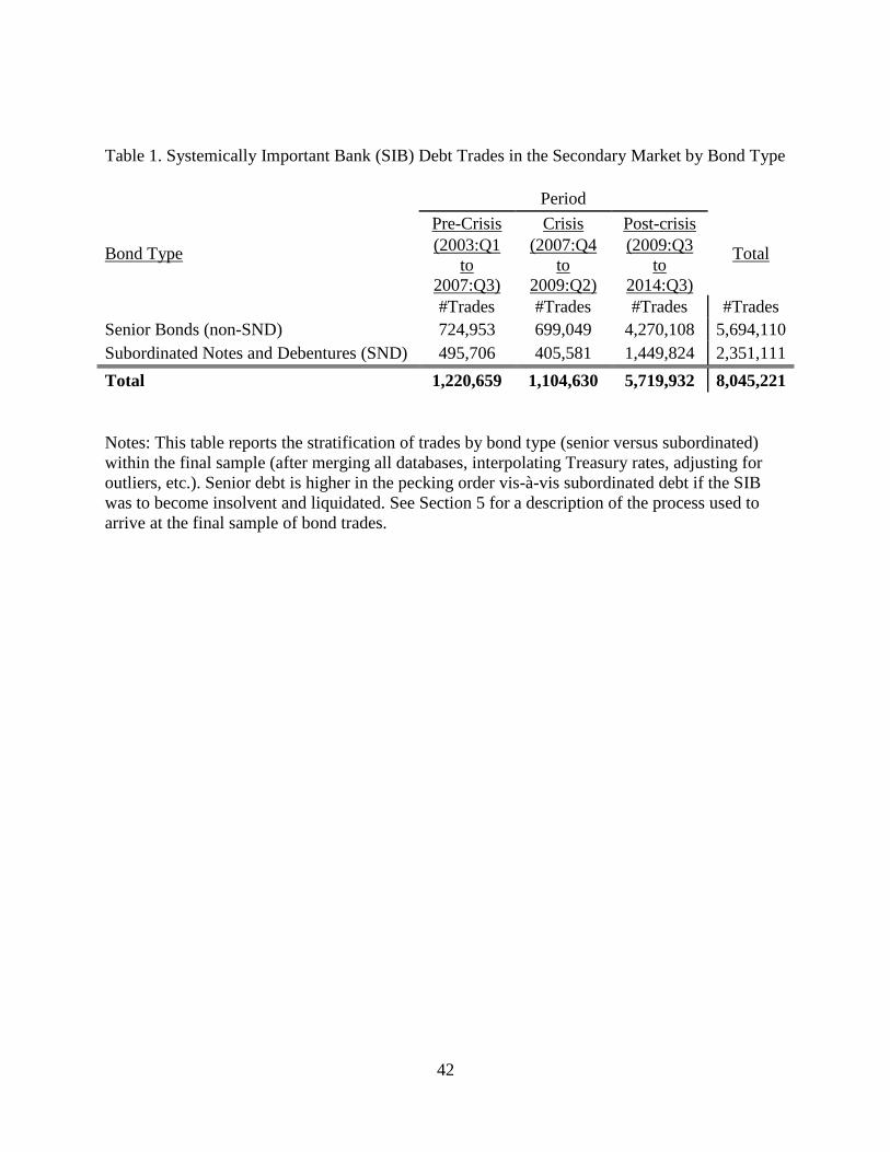
42
Table 1. Systemically Important Bank (SIB) Debt Trades in the Secondary Market by Bond Type
Period
Bond Type
Pre-Crisis Crisis Post-crisis
Total (2003:Q1
to
2007:Q3)
(2007:Q4
to
2009:Q2)
(2009:Q3
to
2014:Q3)
#Trades #Trades #Trades #Trades
Senior Bonds (non-SND) 724,953 699,049 4,270,108 5,694,110
Subordinated Notes and Debentures (SND) 495,706 405,581 1,449,824 2,351,111
Total 1,220,659 1,104,630 5,719,932 8,045,221
Notes: This table reports the stratification of trades by bond type (senior versus subordinated)
within the final sample (after merging all databases, interpolating Treasury rates, adjusting for
outliers, etc.). Senior debt is higher in the pecking order vis-à-vis subordinated debt if the SIB
was to become insolvent and liquidated. See Section 5 for a description of the process used to
arrive at the final sample of bond trades.
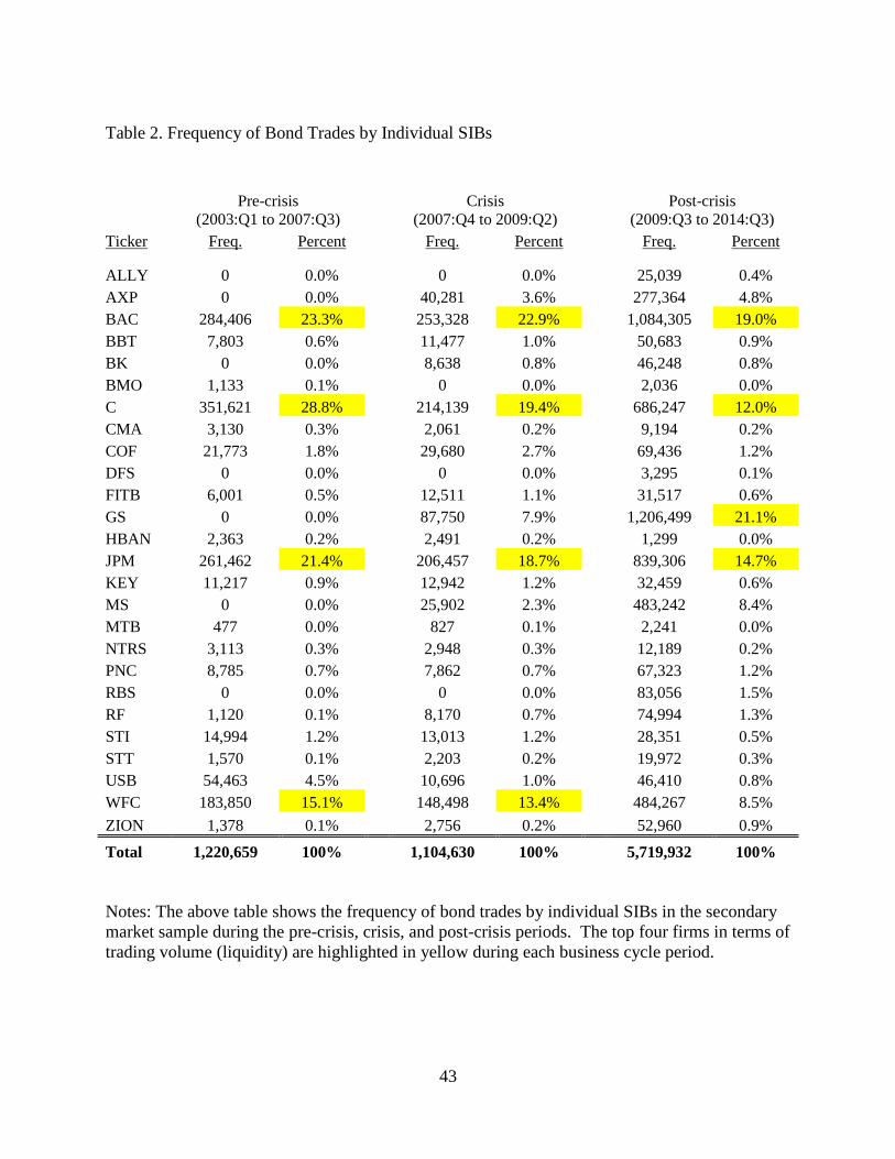
43
Table 2. Frequency of Bond Trades by Individual SIBs
Pre-crisis
(2003:Q1 to 2007:Q3)
Crisis
(2007:Q4 to 2009:Q2)
Post-crisis
(2009:Q3 to 2014:Q3)
Ticker Freq. Percent
Freq. Percent
Freq. Percent
ALLY 0 0.0%
0 0.0%
25,039 0.4%
AXP 0 0.0%
40,281 3.6%
277,364 4.8%
BAC 284,406 23.3%
253,328 22.9%
1,084,305 19.0%
BBT 7,803 0.6%
11,477 1.0%
50,683 0.9%
BK 0 0.0%
8,638 0.8%
46,248 0.8%
BMO 1,133 0.1%
0 0.0%
2,036 0.0%
C 351,621 28.8%
214,139 19.4%
686,247 12.0%
CMA 3,130 0.3%
2,061 0.2%
9,194 0.2%
COF 21,773 1.8%
29,680 2.7%
69,436 1.2%
DFS 0 0.0%
0 0.0%
3,295 0.1%
FITB 6,001 0.5%
12,511 1.1%
31,517 0.6%
GS 0 0.0%
87,750 7.9%
1,206,499 21.1%
HBAN 2,363 0.2%
2,491 0.2%
1,299 0.0%
JPM 261,462 21.4%
206,457 18.7%
839,306 14.7%
KEY 11,217 0.9%
12,942 1.2%
32,459 0.6%
MS 0 0.0%
25,902 2.3%
483,242 8.4%
MTB 477 0.0%
827 0.1%
2,241 0.0%
NTRS 3,113 0.3%
2,948 0.3%
12,189 0.2%
PNC 8,785 0.7%
7,862 0.7%
67,323 1.2%
RBS 0 0.0%
0 0.0%
83,056 1.5%
RF 1,120 0.1%
8,170 0.7%
74,994 1.3%
STI 14,994 1.2%
13,013 1.2%
28,351 0.5%
STT 1,570 0.1%
2,203 0.2%
19,972 0.3%
USB 54,463 4.5%
10,696 1.0%
46,410 0.8%
WFC 183,850 15.1%
148,498 13.4%
484,267 8.5%
ZION 1,378 0.1%
2,756 0.2%
52,960 0.9%
Total 1,220,659 100%
1,104,630 100%
5,719,932 100%
Notes: The above table shows the frequency of bond trades by individual SIBs in the secondary
market sample during the pre-crisis, crisis, and post-crisis periods. The top four firms in terms of
trading volume (liquidity) are highlighted in yellow during each business cycle period.

Table 3. Variables Included in the Analysis
Panel A: SIB-
specific variables Source Units Frequency Definition
lag (Tier 1 Capital
Ratio) FR Y-9C % Quarterly
Tier 1 Capital Ratio (BHC Consolidated) calculated as the:
sum of: total BHC equity capital, qualifying Class A non-controlling (minority) interest in consolidated
subsidiaries, qualifying restricted core capital elements, qualifying mandatory convertible preferred securities
of internationally active BHCs, and other additions to (deductions from) Tier 1 capital,
less: net unrealized gains (losses) on available-for-sale securities, accumulated net gains (losses on cash flow
hedges and amounts recorded in AOCI resulting from the initial and subsequent application of FASB ASC
715-20 to defined benefit postretirement plans, non-qualifying perpetual preferred stock, disallowed goodwill
and other disallowed intangible assets, cumulative change in fair value of all financial liabilities accounted for
under a fair value option that is included in retained earnings and is attributable to changes in the BHC’s own
creditworthiness, disallowed servicing assets and purchased credit card relationships, and disallowed deferred
tax assets
divided by: average total assets for leverage capital purposes
lag (net charge-offs
(NCOs) / Loans) BHCPR % Quarterly Loan & Lease Losses / Average Loans & Leases
lag (Inefficiency
Ratio) BHCPR % Quarterly
The sum of salaries and employee benefits, expense on premises and fixed assets (net of rental income),
amortization expense of intangible assets, and other non-interest expenses (i.e. total noninterest expense)
divided by average assets.*
lag(ROAA) BHCPR % Quarterly Net Income / Average Assets
lag (Liquidity Ratio) BHCPR % Quarterly
Short-term Investments (the sum of interest-bearing bank balances, federal funds sold and securities purchased
under agreements to resell, and debt securities with a remaining maturity of one year or less) / Consolidated
Assets*
lag (Net short-term
(ST) Assets / Assets) BHCPR % Quarterly
The difference between earning assets that are repriceable (mature within one year and the sum of interest-
bearing deposit liabilities that reprice or mature within one year and long-term debt that reprices within one
year divided by total assets.*
lag (assets) FR Y-9C
real $
($000) Quarterly BHC Consolidated Assets
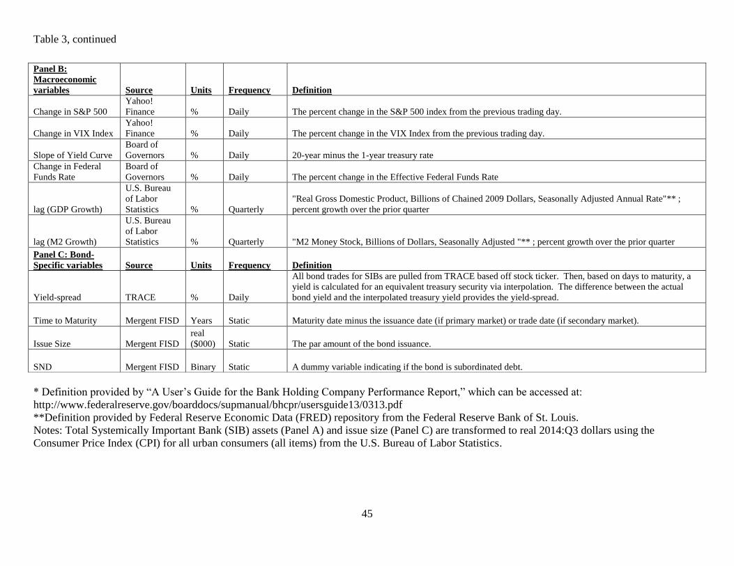
45
Table 3, continued
* Definition provided by “A User’s Guide for the Bank Holding Company Performance Report,” which can be accessed at:
http://www.federalreserve.gov/boarddocs/supmanual/bhcpr/usersguide13/0313.pdf
**Definition provided by Federal Reserve Economic Data (FRED) repository from the Federal Reserve Bank of St. Louis.
Notes: Total Systemically Important Bank (SIB) assets (Panel A) and issue size (Panel C) are transformed to real 2014:Q3 dollars using the
Consumer Price Index (CPI) for all urban consumers (all items) from the U.S. Bureau of Labor Statistics.
Panel B:
Macroeconomic
variables Source Units Frequency Definition
Change in S&P 500
Yahoo!
Finance % Daily The percent change in the S&P 500 index from the previous trading day.
Change in VIX Index
Yahoo!
Finance % Daily The percent change in the VIX Index from the previous trading day.
Slope of Yield Curve
Board of
Governors % Daily 20-year minus the 1-year treasury rate
Change in Federal
Funds Rate
Board of
Governors % Daily The percent change in the Effective Federal Funds Rate
lag (GDP Growth)
U.S. Bureau
of Labor
Statistics % Quarterly
"Real Gross Domestic Product, Billions of Chained 2009 Dollars, Seasonally Adjusted Annual Rate"** ;
percent growth over the prior quarter
lag (M2 Growth)
U.S. Bureau
of Labor
Statistics % Quarterly "M2 Money Stock, Billions of Dollars, Seasonally Adjusted "** ; percent growth over the prior quarter
Panel C: Bond-
Specific variables Source Units Frequency Definition
Yield-spread TRACE % Daily
All bond trades for SIBs are pulled from TRACE based off stock ticker. Then, based on days to maturity, a
yield is calculated for an equivalent treasury security via interpolation. The difference between the actual
bond yield and the interpolated treasury yield provides the yield-spread.
Time to Maturity Mergent FISD Years Static Maturity date minus the issuance date (if primary market) or trade date (if secondary market).
Issue Size Mergent FISD
real
($000) Static The par amount of the bond issuance.
SND Mergent FISD Binary Static A dummy variable indicating if the bond is subordinated debt.
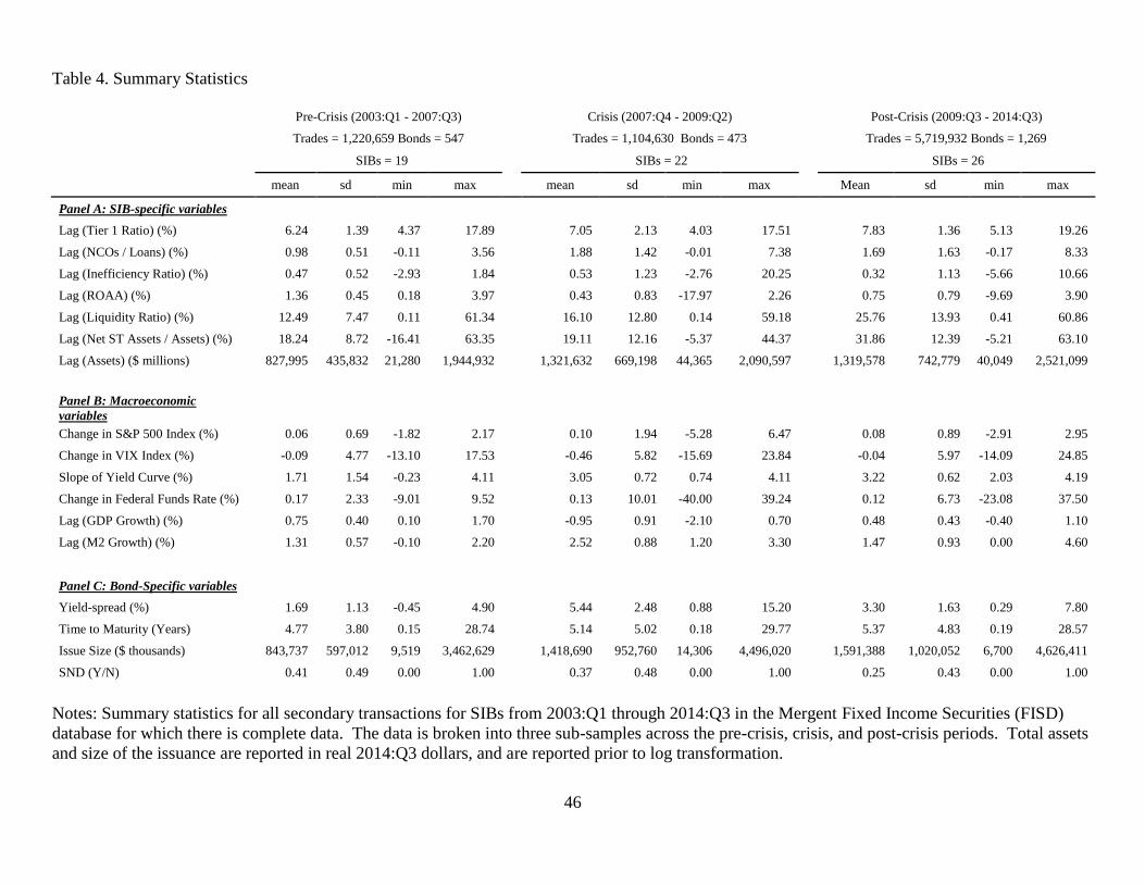
46
Table 4. Summary Statistics
Pre-Crisis (2003:Q1 - 2007:Q3)
Crisis (2007:Q4 - 2009:Q2)
Post-Crisis (2009:Q3 - 2014:Q3)
Trades = 1,220,659 Bonds = 547 Trades = 1,104,630 Bonds = 473 Trades = 5,719,932 Bonds = 1,269
SIBs = 19 SIBs = 22 SIBs = 26
mean sd min max mean sd min max Mean sd min max
Panel A: SIB-specific variables
Lag (Tier 1 Ratio) (%) 6.24 1.39 4.37 17.89
7.05 2.13 4.03 17.51
7.83 1.36 5.13 19.26
Lag (NCOs / Loans) (%) 0.98 0.51 -0.11 3.56
1.88 1.42 -0.01 7.38
1.69 1.63 -0.17 8.33
Lag (Inefficiency Ratio) (%) 0.47 0.52 -2.93 1.84
0.53 1.23 -2.76 20.25
0.32 1.13 -5.66 10.66
Lag (ROAA) (%) 1.36 0.45 0.18 3.97
0.43 0.83 -17.97 2.26
0.75 0.79 -9.69 3.90
Lag (Liquidity Ratio) (%) 12.49 7.47 0.11 61.34
16.10 12.80 0.14 59.18
25.76 13.93 0.41 60.86
Lag (Net ST Assets / Assets) (%) 18.24 8.72 -16.41 63.35
19.11 12.16 -5.37 44.37
31.86 12.39 -5.21 63.10
Lag (Assets) ($ millions) 827,995 435,832 21,280 1,944,932
1,321,632 669,198 44,365 2,090,597
1,319,578 742,779 40,049 2,521,099
Panel B: Macroeconomic
variables
Change in S&P 500 Index (%) 0.06 0.69 -1.82 2.17
0.10 1.94 -5.28 6.47
0.08 0.89 -2.91 2.95
Change in VIX Index (%) -0.09 4.77 -13.10 17.53
-0.46 5.82 -15.69 23.84
-0.04 5.97 -14.09 24.85
Slope of Yield Curve (%) 1.71 1.54 -0.23 4.11
3.05 0.72 0.74 4.11
3.22 0.62 2.03 4.19
Change in Federal Funds Rate (%) 0.17 2.33 -9.01 9.52
0.13 10.01 -40.00 39.24
0.12 6.73 -23.08 37.50
Lag (GDP Growth) (%) 0.75 0.40 0.10 1.70
-0.95 0.91 -2.10 0.70
0.48 0.43 -0.40 1.10
Lag (M2 Growth) (%) 1.31 0.57 -0.10 2.20
2.52 0.88 1.20 3.30
1.47 0.93 0.00 4.60
Panel C: Bond-Specific variables
Yield-spread (%) 1.69 1.13 -0.45 4.90
5.44 2.48 0.88 15.20
3.30 1.63 0.29 7.80
Time to Maturity (Years) 4.77 3.80 0.15 28.74
5.14 5.02 0.18 29.77
5.37 4.83 0.19 28.57
Issue Size ($ thousands) 843,737 597,012 9,519 3,462,629
1,418,690 952,760 14,306 4,496,020
1,591,388 1,020,052 6,700 4,626,411
SND (Y/N) 0.41 0.49 0.00 1.00
0.37 0.48 0.00 1.00
0.25 0.43 0.00 1.00
Notes: Summary statistics for all secondary transactions for SIBs from 2003:Q1 through 2014:Q3 in the Mergent Fixed Income Securities (FISD)
database for which there is complete data. The data is broken into three sub-samples across the pre-crisis, crisis, and post-crisis periods. Total assets
and size of the issuance are reported in real 2014:Q3 dollars, and are reported prior to log transformation.
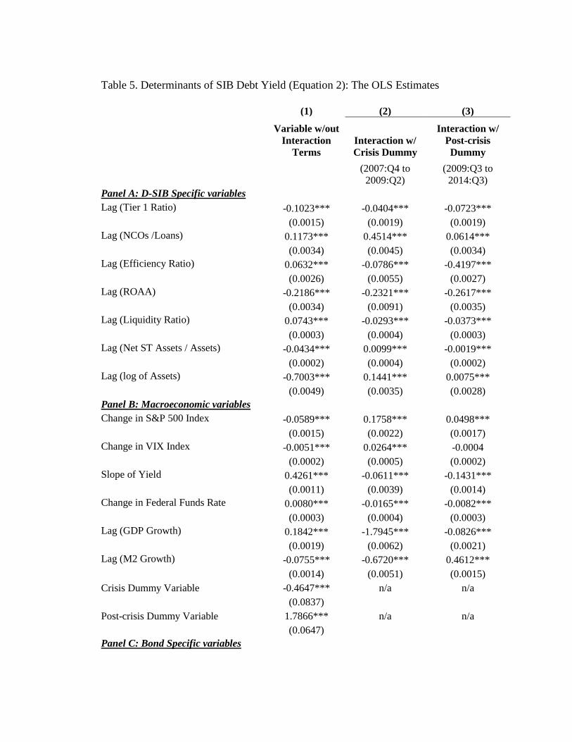
Table 5. Determinants of SIB Debt Yield (Equation 2): The OLS Estimates
(1) (2) (3)
Variable w/out
Interaction
Terms
Interaction w/
Crisis Dummy
Interaction w/
Post-crisis
Dummy
(2007:Q4 to
2009:Q2)
(2009:Q3 to
2014:Q3)
Panel A: D-SIB Specific variables
Lag (Tier 1 Ratio)
-0.1023*** -0.0404*** -0.0723***
(0.0015) (0.0019) (0.0019)
Lag (NCOs /Loans)
0.1173*** 0.4514*** 0.0614***
(0.0034) (0.0045) (0.0034)
Lag (Efficiency Ratio)
0.0632*** -0.0786*** -0.4197***
(0.0026) (0.0055) (0.0027)
Lag (ROAA)
-0.2186*** -0.2321*** -0.2617***
(0.0034) (0.0091) (0.0035)
Lag (Liquidity Ratio)
0.0743*** -0.0293*** -0.0373***
(0.0003) (0.0004) (0.0003)
Lag (Net ST Assets / Assets)
-0.0434*** 0.0099*** -0.0019***
(0.0002) (0.0004) (0.0002)
Lag (log of Assets)
-0.7003*** 0.1441*** 0.0075***
(0.0049) (0.0035) (0.0028)
Panel B: Macroeconomic variables
Change in S&P 500 Index
-0.0589*** 0.1758*** 0.0498***
(0.0015) (0.0022) (0.0017)
Change in VIX Index
-0.0051*** 0.0264*** -0.0004
(0.0002) (0.0005) (0.0002)
Slope of Yield
0.4261*** -0.0611*** -0.1431***
(0.0011) (0.0039) (0.0014)
Change in Federal Funds Rate
0.0080*** -0.0165*** -0.0082***
(0.0003) (0.0004) (0.0003)
Lag (GDP Growth)
0.1842*** -1.7945*** -0.0826***
(0.0019) (0.0062) (0.0021)
Lag (M2 Growth)
-0.0755*** -0.6720*** 0.4612***
(0.0014) (0.0051) (0.0015)
Crisis Dummy Variable -0.4647*** n/a n/a
(0.0837)
Post-crisis Dummy Variable 1.7866*** n/a n/a
(0.0647)
Panel C: Bond Specific variables
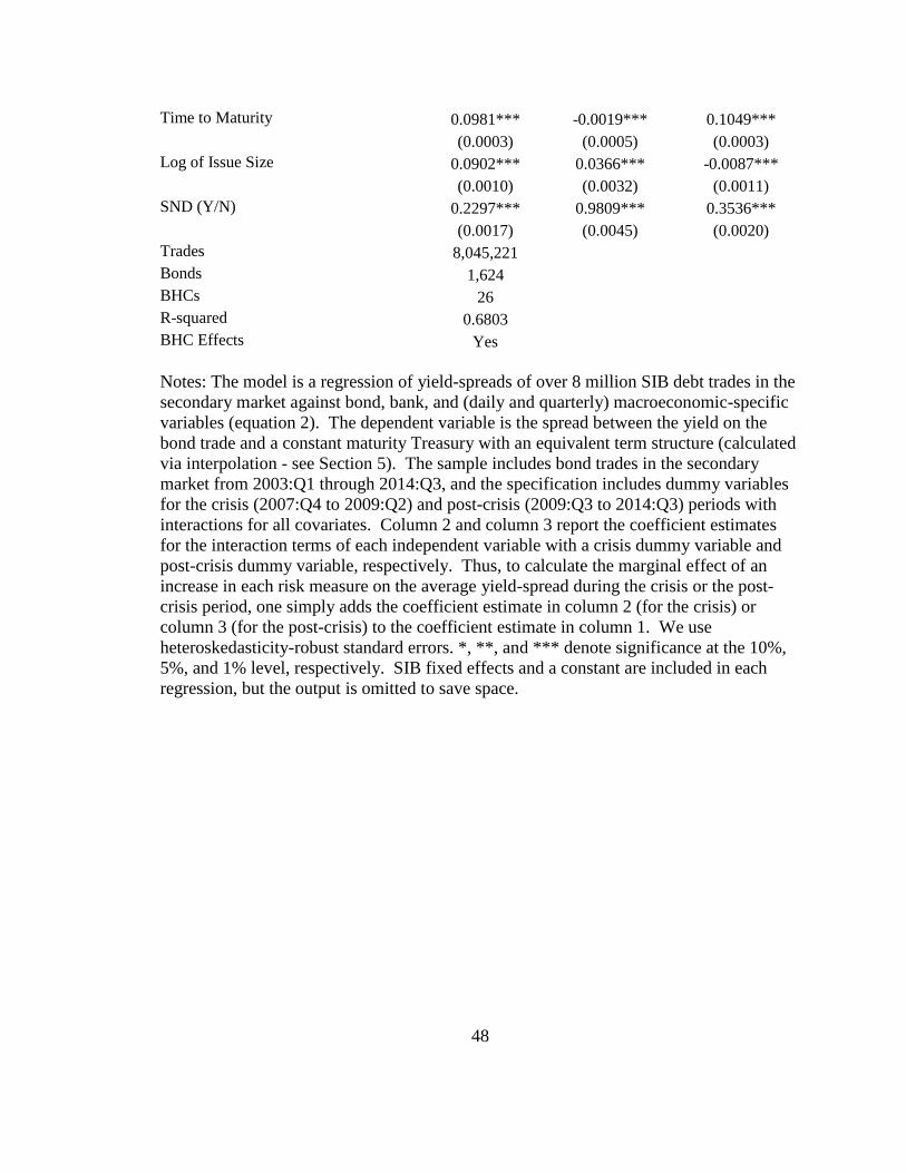
48
Time to Maturity
0.0981*** -0.0019*** 0.1049***
(0.0003) (0.0005) (0.0003)
Log of Issue Size
0.0902*** 0.0366*** -0.0087***
(0.0010) (0.0032) (0.0011)
SND (Y/N)
0.2297*** 0.9809*** 0.3536***
(0.0017) (0.0045) (0.0020)
Trades
8,045,221
Bonds
1,624
BHCs
26
R-squared
0.6803
BHC Effects
Yes
Notes: The model is a regression of yield-spreads of over 8 million SIB debt trades in the
secondary market against bond, bank, and (daily and quarterly) macroeconomic-specific
variables (equation 2). The dependent variable is the spread between the yield on the
bond trade and a constant maturity Treasury with an equivalent term structure (calculated
via interpolation - see Section 5). The sample includes bond trades in the secondary
market from 2003:Q1 through 2014:Q3, and the specification includes dummy variables
for the crisis (2007:Q4 to 2009:Q2) and post-crisis (2009:Q3 to 2014:Q3) periods with
interactions for all covariates. Column 2 and column 3 report the coefficient estimates
for the interaction terms of each independent variable with a crisis dummy variable and
post-crisis dummy variable, respectively. Thus, to calculate the marginal effect of an
increase in each risk measure on the average yield-spread during the crisis or the post-
crisis period, one simply adds the coefficient estimate in column 2 (for the crisis) or
column 3 (for the post-crisis) to the coefficient estimate in column 1. We use
heteroskedasticity-robust standard errors. *, **, and *** denote significance at the 10%,
5%, and 1% level, respectively. SIB fixed effects and a constant are included in each
regression, but the output is omitted to save space.
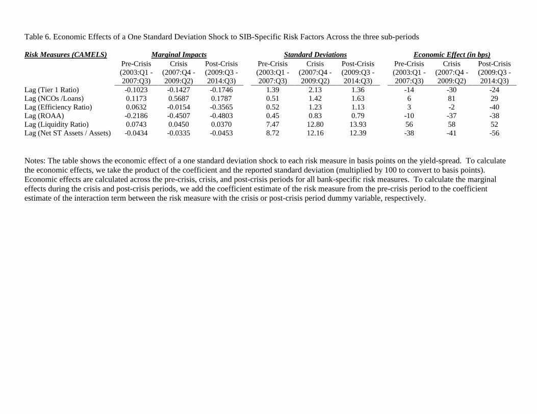
Table 6. Economic Effects of a One Standard Deviation Shock to SIB-Specific Risk Factors Across the three sub-periods
Risk Measures (CAMELS) Marginal Impacts
Standard Deviations
Economic Effect (in bps)
Pre-Crisis
(2003:Q1 -
2007:Q3)
Crisis
(2007:Q4 -
2009:Q2)
Post-Crisis
(2009:Q3 -
2014:Q3)
Pre-Crisis
(2003:Q1 -
2007:Q3)
Crisis
(2007:Q4 -
2009:Q2)
Post-Crisis
(2009:Q3 -
2014:Q3)
Pre-Crisis
(2003:Q1 -
2007:Q3)
Crisis
(2007:Q4 -
2009:Q2)
Post-Crisis
(2009:Q3 -
2014:Q3)
Lag (Tier 1 Ratio) -0.1023 -0.1427 -0.1746
1.39 2.13 1.36
-14 -30 -24
Lag (NCOs /Loans) 0.1173 0.5687 0.1787
0.51 1.42 1.63
6 81 29
Lag (Efficiency Ratio) 0.0632 -0.0154 -0.3565
0.52 1.23 1.13
3 -2 -40
Lag (ROAA) -0.2186 -0.4507 -0.4803
0.45 0.83 0.79
-10 -37 -38
Lag (Liquidity Ratio) 0.0743 0.0450 0.0370
7.47 12.80 13.93
56 58 52
Lag (Net ST Assets / Assets) -0.0434 -0.0335 -0.0453
8.72 12.16 12.39
-38 -41 -56
Notes: The table shows the economic effect of a one standard deviation shock to each risk measure in basis points on the yield-spread. To calculate
the economic effects, we take the product of the coefficient and the reported standard deviation (multiplied by 100 to convert to basis points).
Economic effects are calculated across the pre-crisis, crisis, and post-crisis periods for all bank-specific risk measures. To calculate the marginal
effects during the crisis and post-crisis periods, we add the coefficient estimate of the risk measure from the pre-crisis period to the coefficient
estimate of the interaction term between the risk measure with the crisis or post-crisis period dummy variable, respectively.
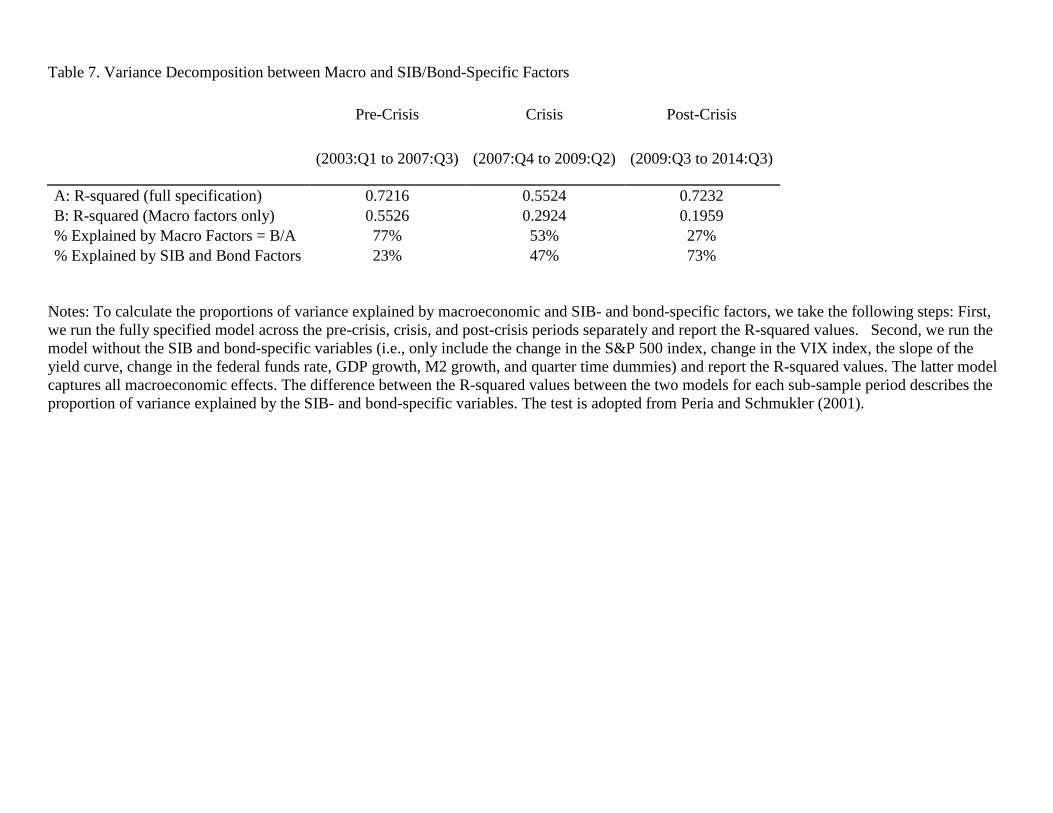
Table 7. Variance Decomposition between Macro and SIB/Bond-Specific Factors
Pre-Crisis Crisis Post-Crisis
(2003:Q1 to 2007:Q3) (2007:Q4 to 2009:Q2) (2009:Q3 to 2014:Q3)
A: R-squared (full specification) 0.7216 0.5524 0.7232
B: R-squared (Macro factors only) 0.5526 0.2924 0.1959
% Explained by Macro Factors = B/A 77% 53% 27%
% Explained by SIB and Bond Factors 23% 47% 73%
Notes: To calculate the proportions of variance explained by macroeconomic and SIB- and bond-specific factors, we take the following steps: First,
we run the fully specified model across the pre-crisis, crisis, and post-crisis periods separately and report the R-squared values. Second, we run the
model without the SIB and bond-specific variables (i.e., only include the change in the S&P 500 index, change in the VIX index, the slope of the
yield curve, change in the federal funds rate, GDP growth, M2 growth, and quarter time dummies) and report the R-squared values. The latter model
captures all macroeconomic effects. The difference between the R-squared values between the two models for each sub-sample period describes the
proportion of variance explained by the SIB- and bond-specific variables. The test is adopted from Peria and Schmukler (2001).

Appendix A. List of U.S. Systemically Important Banks (SIBs)
# SIB Name Ticker Designation
1 Ally Financial ALLY D-SIB
2 American Express Company AXP D-SIB
3 Bank of America BAC G-SIB
4 Bank of New York Mellon BK G-SIB
5 BB&T BBT D-SIB
6 BMO Financial BMO D-SIB
7 Citigroup C G-SIB
8 Comerica CMA D-SIB
9 Capital One Financial COF D-SIB
10 Discover Financial Services DFS D-SIB
11 Fifth Third Bancorp FITB D-SIB
12 Goldman Sachs GS G-SIB
13 Huntington Bancshares HBAN D-SIB
14 JP Morgan Chase JPM G-SIB
15 KeyCorp KEY D-SIB
16 Morgan Stanley MS G-SIB
17 M&T Bank MTB D-SIB
18 Northern Trust NTRS D-SIB
19 PNC Financial Services Group PNC D-SIB
20 Royal Bank of Scotland Group RBS D-SIB
21 Regions Financial RF D-SIB
22 State Street STT G-SIB
23 SunTrust Banks STI D-SIB
24 U.S. Bancorp USB D-SIB
25 Wells Fargo WFC G-SIB
26 Zions Bancorporation ZION D-SIB
Notes: The designation listed above stands for Global or Domestic Systemically
Important Bank (G-SIB or D-SIB, respectively).
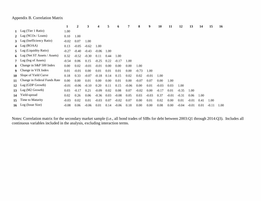
Appendix B. Correlation Matrix
1 2 3 4 5 6 7 8 9 10 11 12 13 14 15 16
1 Lag (Tier 1 Ratio) 1.00
2 Lag (NCOs / Loans) 0.10 1.00
3 Lag (Inefficiency Ratio) -0.02 0.07 1.00
4 Lag (ROAA) 0.13 -0.05 -0.62 1.00
5 Lag (Liquidity Ratio) -0.27 -0.40 -0.43 -0.06 1.00
6 Lag (Net ST Assets / Assets) 0.32 -0.52 -0.30 0.11 0.44 1.00
7 Lag (log of Assets) -0.54 0.06 0.15 -0.25 0.22 -0.17 1.00
8 Change in S&P 500 Index 0.00 0.02 -0.01 -0.01 0.00 0.00 0.00 1.00
9 Change in VIX Index 0.01 -0.01 0.00 0.01 0.01 0.01 0.00 -0.73 1.00
10 Slope of Yield Curve 0.18 0.33 -0.07 -0.18 0.14 0.15 0.02 0.02 -0.01 1.00
11 Change in Federal Funds Rate 0.00 0.00 0.01 0.00 0.00 0.01 0.00 -0.07 0.07 0.00 1.00
12 Lag (GDP Growth) -0.01 -0.06 -0.10 0.20 0.11 0.15 -0.06 0.00 0.01 -0.03 0.03 1.00
13 Lag (M2 Growth) 0.03 -0.17 0.21 -0.09 0.02 0.08 0.07 -0.02 0.00 -0.17 0.01 -0.35 1.00
14 Yield-spread 0.02 0.26 0.06 -0.36 0.03 -0.08 0.05 0.03 -0.03 0.37 -0.01 -0.31 0.06 1.00
15 Time to Maturity -0.03 0.02 0.01 -0.03 0.07 -0.02 0.07 0.00 0.01 0.02 0.00 0.01 -0.01 0.41 1.00
16 Log (Issue Size) -0.08 0.06 -0.06 0.01 0.14 -0.06 0.18 0.00 0.00 0.08 0.00 -0.04 -0.01 0.01 -0.11 1.00
Notes: Correlation matrix for the secondary market sample (i.e., all bond trades of SIBs for debt between 2003:Q1 through 2014:Q3). Includes all
continuous variables included in the analysis, excluding interaction terms.