Market Externalities of Large Unemployment Insurance

Market Externalities of LargeUnemployment Insurance Extensions

Rafael Lalive, Camille Landais & Josef Zweimuller

CRESTDecember 24, 2012

Camille Landais - LSE (CREST 12/2012) UI externalities 1 / 29

Motivation:

What is the effect of increasing generosity of UIon labor market outcomes?

We ≈ know what micro effect isI In theory, increase in UI unambiguously increase U

duration

I Empirically, large number of well-identified microestimates

What about macro effect?I In theory, large literature on equilibrium search &

matching, but anything goes regarding externalities

I Empirically, difficulty of estimating G-E effects of UI andto analyze how micro and macro estimates differ


UI and labor market externalities:

Market externality:Whenever (UI induced) variations in the searcheffort of some unemployed affect job findingprobability of other unemployed in the same labormarket

Market externality 6= incidence:In market with frictions, efficiency is usually notachieved, so that (UI induced) variations inbehaviors have first order welfare effects


This paper:

Regional Extended Benefit Progam (REBP): Largeextensions of UI in Austria

I Unique quasi-experimental setting to identify marketexternalities

I Strong evidence of positive effects of REBP on untreatedworkers in treated labor markets

Discuss how evidence relates to different search &matching models:

I Evidence refutes predictions of Nash bargaining / flexiblewage models

I Evidence in line with job-rationing models


Related literature:

Theoretical literature on pecuniary externalities:I Geanakoplos & Polemarchakis (1986), etc.

Literature on optimal UI:I Direct continuity of LMS (2012)

Empirical literature on identification of spillovers ofpolicy interventions

I General literature on spillovers: Duflo & Saez (2003)

I Spillovers of active labor market policies: Crepon & al.(2012), Ferracci & al. (2010), Blundell, & al. (2004).

I Spillovers of UI: Levine (1993)


1 Introduction

2 Conceptual framework

3 Institutional background

4 Empirical strategy

5 Results

6 Calibrations


Labor Market with Matching Frictions

u unemployed workers:I Exert search effort eI e function of wedge in consumption ∆c = ce − cu

v vacancies.

Number of matches: m(e · u, v) = ωm · (e · u)η · v 1−η

Labor market tightness: θ ≡ v/(e · u)

Job-finding proba: e · f (θ) = e ·m(1, θ).

Vacancy-filling proba: q(θ) = m (1/θ, 1).




v vacancies.




⇒ ∂e·f (θ)∂θ > 0





v vacancies.





⇒ ∂q(θ)∂θ < 0


Labor market equilibrium

Aggregate labor supply (from equality of in- andoutflows into employment):

ns(e(θ,∆c), θ)

Aggregate labor demand (from firm’s maximisationprogram):

nd(θ)

Labor market equilibrium:

nd(θ) = ns(e(θ,∆c), θ)




ns(e(θ,∆c), θ)


nd(θ)






ns(e(θ,∆c), θ)


nd(θ)






ns(e(θ,∆c), θ)


nd(θ)




Figure 1 : Externalities in a model with Nash bargaining

Employment n

La

bo

r m

ark

et tightn

ess θ

Supply: high UISupply: low UIDemand: high UIDemand: low UI

B

εm

εM

A

C

Figure 2 : Labor market equilibrium in a Michaillat model

Employment n

La

bo

r m

ark

et tightn

ess θ

Supply: high UISupply: low UIDemand: expansion

CA

εM

B

εm

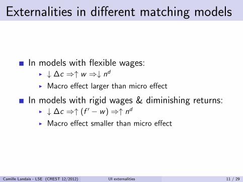
Externalities in different matching models

In models with flexible wages:I ↓ ∆c ⇒↑ w ⇒↓ nd

I Macro effect larger than micro effect

In models with rigid wages & diminishing returns:I ↓ ∆c ⇒↑ (f ′ − w)⇒↑ nd

I Macro effect smaller than micro effect


1 Introduction

2 Conceptual framework

3 Institutional background

4 Empirical strategy

5 Results

6 Calibrations


REBP reform in Austria

Large UI benefit extension program enacted inAustria

I 209 weeks instead of 52 weeks

Eligibility requirements:I Age: more than 50

I Reside in selected regions at least 6 months beforebecoming unemployed

I At least 15 years of continuous work history in the past25 years

I Spell beginning between June 1988 and Dec 1993


Figure 3 : Austrian regions by REBP treatment status

90 0 9045 Kilometers

With Extended Benefits = Shaded

Without Extended Benefits = White

Data:

Universe of UI spells in Austria from 1980 to 2010:I Info on age, residence, education, marital status, etc...

Universe of social security data in Austria from 1949to 2010:

I Info on each employment spell

I Compute experience in past 25 years

I Merge with UI data to determine REBP eligibility

I Info on wages, industry, tenure,


Sample selection:

Endogeneity of choice of REBP regions:I Regions are not selected at random: restructuring of

steel sector

I Remove all steel sector workers (at most 15% ofunemployed in treated regions), and all workers in relatedindustries

Early retirement programs:I Women can go directly from REBP to early retirement

programs

I We focus only on men 50 to 54 bc they cannot godirectly from REBP to early retirement


Empirical strategy:

First stage: Compare treated workers in treatedregions and untreated regions before/during/after

Second stage: Compare untreated workers intreated and untreated regions before/during/after

Identification assumptions:I Treated and untreated regions are somehow isolated

I Unobserved differences between treated and untreatedworkers fixed over time

I Unobserved differences between labor markets are fixedover time


Table 1 : Summary statistics:

(1) (2) (3) (4)

A. All workerstreated vs untreated counties before 1988

M=0 M=1 Difference p-value

Age 51.9 51.9 0 .366

U duration 18.7 19.4 -.7 .12

Non employment duration 31.7 29.9 1.8 .018

Fraction spells > 100 wks .033 .039 -.006 .023

Fraction spells >26 wks .135 .122 .013 .016

Real wage before spell 52.1 50.5 1.6 0

Real wage after spell 51.8 50.8 1.1 0

White Collar .063 .035 .028 0

Fraction not in construction .38 .369 .011 .148

B. Treated workers vs untreated workersin treated counties before 1988

T=0 T=1 Difference p-value

Age 51.8 51.9 -.1 .181

Experience 4089.365 8292.634 -4203.269 0

U duration 16.3 19.6 -3.3 .025

Non employment duration 52.5 28 24.5 0



Real wage before spell 47.3 50.8 -3.6 0

Real wag after spell 47.4 51 -3.6 0

White Collar .01 .037 -.027 .006

Fraction not in construction .345 .371 -.026 .307

Figure 4 : Local labor markets integration: Fraction of newhires from REBP regions in total number of new hires by county

No data0−4% of new hires coming from REBP regions4−20% of new hires coming from REBP regions20−100% of new hires coming from REBP regionsREBP regions

Sample: male age 50 to 54 in non steel-related industries, 1980-1987.

Figure 5 : Difference in U duration between REBP and nonREBP regions: male 50-54 with more than 15 years of experience

First entryinto REBP

Last entryinto REBP

Endof REBP

−20

020

40

60

80

100

weeks

1980 1985 1990 1995 2000 2005 2010

Figure 6 : Difference in U duration between REBP and nonREBP regions: male 50-54 with less than 15 years of experience

First entryinto REBP

Last entryinto REBP

Endof REBP

−40

−20

020

40

weeks

1980 1985 1990 1995 2000 2005 2010

Baseline specifications:

Yirt = α +

Effect of REBP on treated︷︸︸︷β0 · Zirt · Rr · Tt +

Effect of REBP on non-treated︷︸︸︷γ0 · (1− Zirt) · Rr · Tt

+η0Rr + η1Birt + η2Birt · Rr

+∑

νt +∑

η3Birt · ιt + X ′itρ + εirt

Rr : indicator for residing in REBP region

Tt : indicator for spell starting btw June 1988 and Dec 1997

Birt = 1[exp > 15]: indicator for more than 15 yrs of exp

Zirt = Birt · T̃t : indicator for being eligible to REBP extensions


Table 2 : Baseline estimates of the treatment effect of REBP ontreated unemployed and untreated unemployed

(1) (2) (3) (4) (5) (6) (7)

Unemployment duration Non-empl. Spell Spell

duration >100 wks >26 wks

β0 62.41*** 54.57*** 55.48*** 58.14*** 26.03*** 0.233*** 0.236***

(9.565) (8.345) (9.051) (9.159) (5.797) (0.0312) (0.0290)

γ0 -6.941*** -7.165*** -11.86*** -8.979*** -9.725*** -0.0186*** -0.0297**

(1.690) (2.017) (1.640) (1.433) (1.487) (0.00509) (0.0116)

Educ., marital status,

industry, citizenship × × × × × ×

Preexisting trendsby region ×by region×exp × × × ×

N 127802 126091 126091 126091 106164 126091 126091

S.e. clustered at the year×region level in parentheses. * p<0.10, ** p<0.05, *** p<0.010.

Potential confounders:

Confounder 1: selectionI Self-selection into unemployment affected by the reform

for non-treated group in treated counties

I If anything, bias likely to attenuate estimate of spillovereffect on non-treated

Confounder 2: differential region-specific shocks

I REBP regions experience positive shock on labor marketconditions at the time REBP was implemented

I If anything, we expect negative shock if REBP regionsendogenously selected


Table 3 : Testing for selection: inflow rate into unemployment andlog real wage in previous job

(1) (2) (3)

log separation log real wage

rate in previous job

eligible 0.287***

(0.0355)

non-eligible -0.0346

(0.0306)

β0 0.144** 0.132**

(0.0691) (0.0614)

γ0 -0.0638 -0.0479

(0.0629) (0.0608)

N 1733 114770 112242

Standard errors in parentheses, * p<0.10, ** p<0.05, *** p<0.010

Table 4 : Using regions close to REBP border with high labormarket integration as spillover group

(1) (2) (3) (4) (5) (6)

Unemployment duration Non-empl. Spell Spell

duration >100 wks >26 wks

β0 66.20*** 58.24*** 65.09*** 27.68*** 0.254*** 0.251***

(10.13) (8.865) (9.869) (6.298) (0.0339) (0.0316)

γ0 -1.813 -1.588 -3.110 -3.446 -0.0117 -0.0602**

(3.323) (2.954) (3.261) (2.563) (0.0118) (0.0257)


industry, citizenship × × × × ×

Preexisting trendsby region × × × ×

N 160714 157578 159104 135702 159104 159104

S.e. clustered at the year×region level in parentheses. * p<0.10, ** p<0.05, *** p<0.010

Table 5 : Effects of REBP on subsequent wages and match quality

(1) (2) (3) (4) (5) (6)

log real wage wage drop distance

in next job from next to previous to next job

job (min)

β0 -0.0236 -0.0381** -0.157 -0.0904 -0.456 0.223

(0.0154) (0.0152) (0.214) (0.208) (0.554) (0.549)

γ0 0.00515 -0.0477 0.269 0.462 -0.233 2.476*

(0.0448) (0.0441) (0.591) (0.562) (1.138) (1.240)


industry, citizenship × × ×

N 90345 88634 94503 92719 103678 101715

Standard errors in parentheses. * p<0.10, ** p<0.05, *** p<0.010

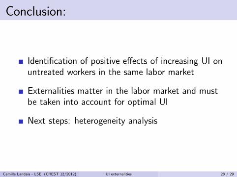
Conclusion:

Identification of positive effects of increasing UI onuntreated workers in the same labor market

Externalities matter in the labor market and mustbe taken into account for optimal UI

Next steps: heterogeneity analysis


Figure 7 : Local labor markets integration: Fraction of newhires from non-REBP regions in total number of new hires by county

No data0−20% of new hires coming from non−REBP regions20−50% of new hires coming from non−REBP regions50−100% of new hires coming from non−REBP regionsnon−REBP regions

Documents

Market Externalities of Large Unemployment Insurance