Market Forces: Demand and Supply - testbanklib.com · of the National Bank of Poland; ... The Web site for the eighth edition of Managerial Eco- ... 76 Managerial Economics and Business

Confirming Pages

Samsung and Hynix Semiconductorto Cut Chip ProductionSam Robbins, owner and CEO of PC Solutions,arrived at the office and glanced at the front pageof The Wall Street Journal waiting on his desk.One of the articles contained statements from exec-utives of two of South Korea’s largest semiconduc-tor manufacturers—Samsung Electronic Companyand Hynix Semiconductor—indicating that theywould suspend all their memory chip productionfor one week. The article went on to say thatanother large semiconductor manufacturer waslikely to follow suit. Collectively, these three chipmanufacturers produce about 30 percent of theworld’s basic semiconductor chips.

PC Solutions is a small but growing company thatassembles PCs and sells them in the highly competitivemarket for “clones.” PC Solutions experienced 100 per-cent growth last year and is in the process of interview-ing recent graduates in an attempt to double itsworkforce.

After reading the article, Sam picked up the phoneand called a few of his business contacts to verify for himself the information contained in theJournal. Satisfied that the information was correct, he called the director of personnel, JaneRemak.

What do you think Sam and Jane discussed?

CH

APTE

RTW

O

HEADLINE

Market Forces: Demand and Supply

Learning ObjectivesAfter completing this chapter, you will be able to:

LO1 Explain the laws of demand and supply,and identify factors that cause demandand supply to shift.

LO2 Calculate consumer surplus and producersurplus, and describe what they mean.

LO3 Explain price determination in a competitive market, and show how equilibrium changes in response tochanges in determinants of demand and supply.

LO4 Explain and illustrate how excise taxes,ad valorem taxes, price floors, andprice ceilings impact the functioning ofa market.

LO5 Apply supply and demand analysis as aqualitative forecasting tool to see the “bigpicture” in competitive markets.

37

bay23224_ch02_037-076.qxd 12/14/12 10:04 AM Page 37

Confirming Pages

38 Managerial Economics and Business Strategy

INTRODUCTION

This chapter describes supply and demand, which are the driving forces behind themarket economies that exist in the United States and around the globe. As sug-gested in this chapter’s opening headline, supply and demand analysis is a tool thatmanagers can use to visualize the “big picture.” Many companies fail because theirmanagers get bogged down in the day-to-day decisions of the business withouthaving a clear picture of market trends and changes that are on the horizon.

To illustrate, imagine that you manage a small retail outlet that sells PCs. A magicgenie appears and says, “Over the next month, the market price of PCs will decline andconsumers will purchase fewer PCs.” The genie revealed the big picture: PC pricesand sales will decline. If you worry about the details of your business without knowl-edge of these future trends in prices and sales, you will be at a significant competitivedisadvantage. Absent a view of the big picture, you are likely to negotiate the wrongprices with suppliers and customers, carry too much inventory, hire too many employ-ees, and—if your business spends money on informative advertising—purchase ads inwhich your prices are no longer competitive by the time they reach print.

Supply and demand analysis is a qualitative tool which, like the above genie,empowers managers by enabling them to see the “big picture.” It is a qualitative fore-casting tool you can use to predict trends in competitive markets, including changes in theprices of your firm’s products, related products (both substitutes and complements),and the prices of inputs (such as labor services) that are necessary for your operations.As we will see in subsequent chapters, after you use supply and demand analysis tosee the big picture, additional tools are available to assist with details—determininghow much the price will change, how much sales and revenues will change, and so on.

For those of you who have taken a principles-level course in economics, someparts of this chapter will be a review. However, make sure you have complete mas-tery of the tools of supply and demand. The rest of this book will assume you havea thorough working knowledge of the material in this chapter.

DEMAND

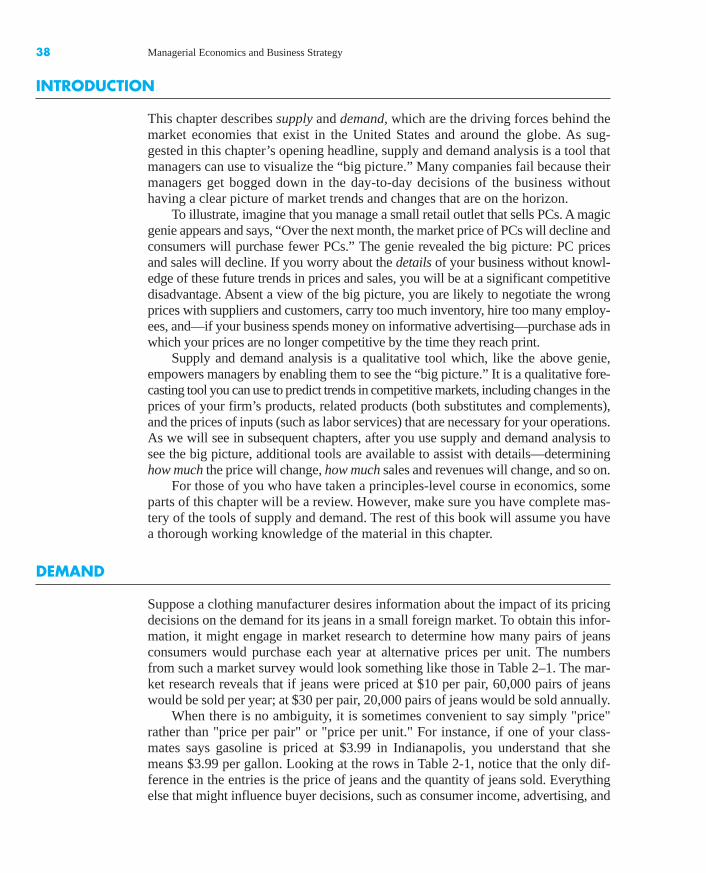
Suppose a clothing manufacturer desires information about the impact of its pricingdecisions on the demand for its jeans in a small foreign market. To obtain this infor-mation, it might engage in market research to determine how many pairs of jeansconsumers would purchase each year at alternative prices per unit. The numbersfrom such a market survey would look something like those in Table 2–1. The mar-ket research reveals that if jeans were priced at $10 per pair, 60,000 pairs of jeanswould be sold per year; at $30 per pair, 20,000 pairs of jeans would be sold annually.

When there is no ambiguity, it is sometimes convenient to say simply "price"rather than "price per pair" or "price per unit." For instance, if one of your class-mates says gasoline is priced at $3.99 in Indianapolis, you understand that shemeans $3.99 per gallon. Looking at the rows in Table 2-1, notice that the only dif-ference in the entries is the price of jeans and the quantity of jeans sold. Everythingelse that might influence buyer decisions, such as consumer income, advertising, and

bay23224_ch02_037-076.qxd 12/14/12 10:04 AM Page 38

Confirming Pages

0

Price ($)

Quantity(thousands per year)10 20 30 40 50 60 70 80

5

10

15

20

25

30

35

40

D

FIGURE 2–1 The Demand Curve

Chapter 2: Market Forces: Demand and Supply 39Chapter 2: Market Forces: Demand and Supply 39

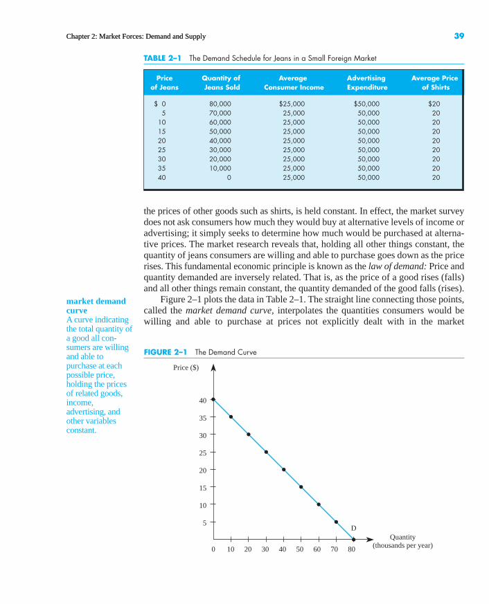
TABLE 2–1 The Demand Schedule for Jeans in a Small Foreign Market

Price Quantity of Average Advertising Average Priceof Jeans Jeans Sold Consumer Income Expenditure of Shirts

$ 0 80,000 $25,000 $50,000 $205 70,000 25,000 50,000 20

10 60,000 25,000 50,000 2015 50,000 25,000 50,000 2020 40,000 25,000 50,000 2025 30,000 25,000 50,000 2030 20,000 25,000 50,000 2035 10,000 25,000 50,000 2040 0 25,000 50,000 20

the prices of other goods such as shirts, is held constant. In effect, the market surveydoes not ask consumers how much they would buy at alternative levels of income oradvertising; it simply seeks to determine how much would be purchased at alterna-tive prices. The market research reveals that, holding all other things constant, thequantity of jeans consumers are willing and able to purchase goes down as the pricerises. This fundamental economic principle is known as the law of demand: Price andquantity demanded are inversely related. That is, as the price of a good rises (falls)and all other things remain constant, the quantity demanded of the good falls (rises).

Figure 2–1 plots the data in Table 2–1. The straight line connecting those points,called the market demand curve, interpolates the quantities consumers would bewilling and able to purchase at prices not explicitly dealt with in the market

market demandcurveA curve indicatingthe total quantity ofa good all con-sumers are willingand able topurchase at eachpossible price,holding the pricesof related goods,income,advertising, andother variablesconstant.

bay23224_ch02_037-076.qxd 12/14/12 10:04 AM Page 39

Confirming Pages

0

Price

Quantity

D1

A

B

D0

D2

Decreasein

demand

Increasein

demand

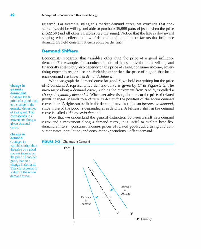
FIGURE 2–2 Changes in Demand

40 Managerial Economics and Business Strategy40 Managerial Economics and Business Strategy

change inquantitydemandedChanges in theprice of a good leadto a change in thequantity demandedof that good. Thiscorresponds to amovement along agiven demandcurve.

research. For example, using this market demand curve, we conclude that con-sumers would be willing and able to purchase 35,000 pairs of jeans when the priceis $22.50 (and all other variables stay the same). Notice that the line is downwardsloping, which reflects the law of demand, and that all other factors that influencedemand are held constant at each point on the line.

Demand Shifters

Economists recognize that variables other than the price of a good influencedemand. For example, the number of pairs of jeans individuals are willing andfinancially able to buy also depends on the price of shirts, consumer income, adver-tising expenditures, and so on. Variables other than the price of a good that influ-ence demand are known as demand shifters.

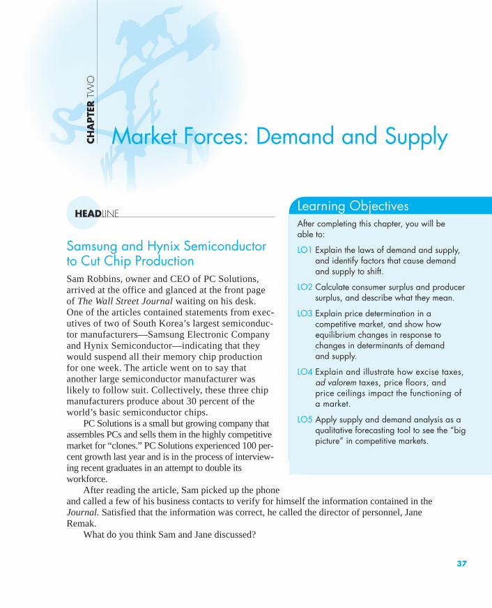
When we graph the demand curve for good X, we hold everything but the priceof X constant. A representative demand curve is given by D0 in Figure 2–2. Themovement along a demand curve, such as the movement from A to B, is called achange in quantity demanded. Whenever advertising, income, or the price of relatedgoods changes, it leads to a change in demand; the position of the entire demandcurve shifts. A rightward shift in the demand curve is called an increase in demand,since more of the good is demanded at each price. A leftward shift in the demandcurve is called a decrease in demand.

Now that we understand the general distinction between a shift in a demandcurve and a movement along a demand curve, it is useful to explain how fivedemand shifters—consumer income, prices of related goods, advertising and con-sumer tastes, population, and consumer expectations—affect demand.

change indemandChanges invariables other thanthe price of a good,such as income orthe price of anothergood, lead to achange in demand.This corresponds toa shift of the entiredemand curve.

bay23224_ch02_037-076.qxd 12/14/12 10:04 AM Page 40

Confirming Pages

INSIDE BUSINESS 2–1

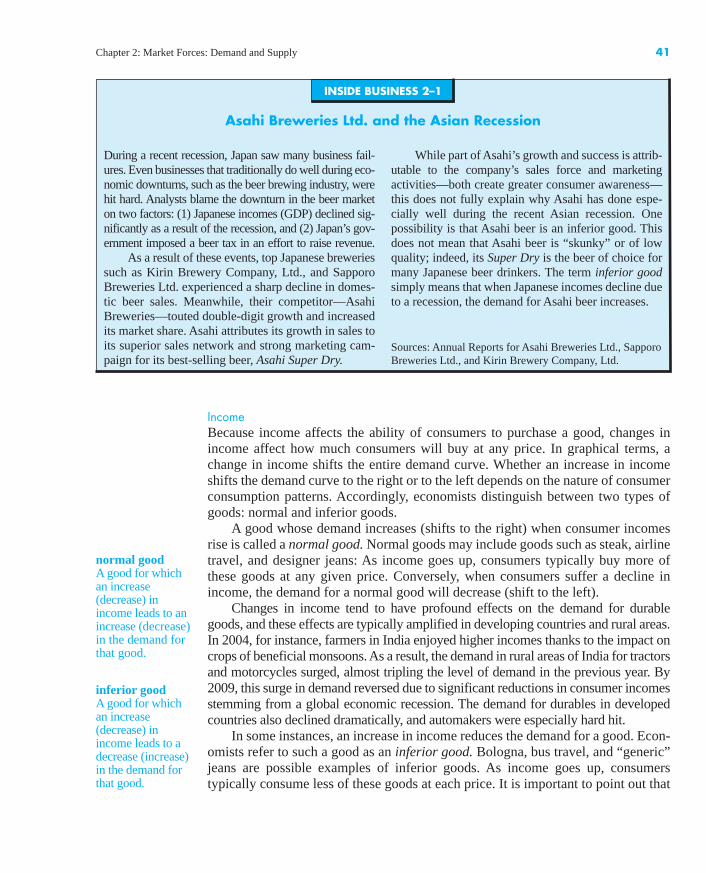
Asahi Breweries Ltd. and the Asian Recession

During a recent recession, Japan saw many business fail-ures. Even businesses that traditionally do well during eco-nomic downturns, such as the beer brewing industry, werehit hard. Analysts blame the downturn in the beer marketon two factors: (1) Japanese incomes (GDP) declined sig-nificantly as a result of the recession, and (2) Japan’s gov-ernment imposed a beer tax in an effort to raise revenue.

As a result of these events, top Japanese breweriessuch as Kirin Brewery Company, Ltd., and SapporoBreweries Ltd. experienced a sharp decline in domes-tic beer sales. Meanwhile, their competitor—AsahiBreweries—touted double-digit growth and increasedits market share. Asahi attributes its growth in sales toits superior sales network and strong marketing cam-paign for its best-selling beer, Asahi Super Dry.

While part of Asahi’s growth and success is attrib-utable to the company’s sales force and marketingactivities—both create greater consumer awareness—this does not fully explain why Asahi has done espe-cially well during the recent Asian recession. Onepossibility is that Asahi beer is an inferior good. Thisdoes not mean that Asahi beer is “skunky” or of lowquality; indeed, its Super Dry is the beer of choice formany Japanese beer drinkers. The term inferior goodsimply means that when Japanese incomes decline dueto a recession, the demand for Asahi beer increases.

Sources: Annual Reports for Asahi Breweries Ltd., SapporoBreweries Ltd., and Kirin Brewery Company, Ltd.

Chapter 2: Market Forces: Demand and Supply 41

normal goodA good for whichan increase(decrease) inincome leads to anincrease (decrease)in the demand forthat good.

inferior goodA good for whichan increase(decrease) inincome leads to adecrease (increase)in the demand forthat good.

IncomeBecause income affects the ability of consumers to purchase a good, changes inincome affect how much consumers will buy at any price. In graphical terms, achange in income shifts the entire demand curve. Whether an increase in incomeshifts the demand curve to the right or to the left depends on the nature of consumerconsumption patterns. Accordingly, economists distinguish between two types ofgoods: normal and inferior goods.

A good whose demand increases (shifts to the right) when consumer incomesrise is called a normal good. Normal goods may include goods such as steak, airlinetravel, and designer jeans: As income goes up, consumers typically buy more ofthese goods at any given price. Conversely, when consumers suffer a decline inincome, the demand for a normal good will decrease (shift to the left).

Changes in income tend to have profound effects on the demand for durablegoods, and these effects are typically amplified in developing countries and rural areas.In 2004, for instance, farmers in India enjoyed higher incomes thanks to the impact oncrops of beneficial monsoons. As a result, the demand in rural areas of India for tractorsand motorcycles surged, almost tripling the level of demand in the previous year. By2009, this surge in demand reversed due to significant reductions in consumer incomesstemming from a global economic recession. The demand for durables in developedcountries also declined dramatically, and automakers were especially hard hit.

In some instances, an increase in income reduces the demand for a good. Econ-omists refer to such a good as an inferior good. Bologna, bus travel, and “generic”jeans are possible examples of inferior goods. As income goes up, consumers typically consume less of these goods at each price. It is important to point out that

bay23224_ch02_037-076.qxd 12/14/12 10:04 AM Page 41

Confirming Pages


by calling such goods inferior, we do not imply that they are of poor quality; we usethis term simply to define products that consumers purchase less of when theirincomes rise and purchase more of when their incomes fall.

Prices of Related GoodsChanges in the prices of related goods generally shift the demand curve for a good.For example, if the price of a Coke increases, most consumers will begin to substi-tute Pepsi, because the relative price of Coke is higher than before. As more andmore consumers substitute Pepsi for Coke, the quantity of Pepsi demanded at eachprice will tend to increase. In effect, an increase in the price of Coke increases thedemand for Pepsi. This is illustrated by a shift in the demand for Pepsi to the right.Goods that interact in this way are known as substitutes.

Many pairs of goods readily come to mind when we think of substitutes: chickenand beef, cars and trucks, raincoats and umbrellas. Such pairs of goods are substitutesfor most consumers. However, substitutes need not serve the same function. Forexample, televisions and patio furniture could be substitutes; as the price of televi-sions increases, you may choose to purchase additional patio furniture rather than anadditional television. Goods are substitutes when an increase in the price of one goodincreases the demand for the other good.

Not all goods are substitutes; in fact, an increase in the price of a good such ascomputer software may lead consumers to purchase fewer computers at each price.Goods that interact in this manner are called complements. Beer and pretzels areanother example of complementary goods. If the price of beer increased, most beerdrinkers would decrease their consumption of pretzels. Notice that when good X isa complement to good Y, a reduction in the price of Y actually increases (shifts tothe right) the demand for good X. More of good X is purchased at each price due tothe reduction in the price of the complement, good Y.

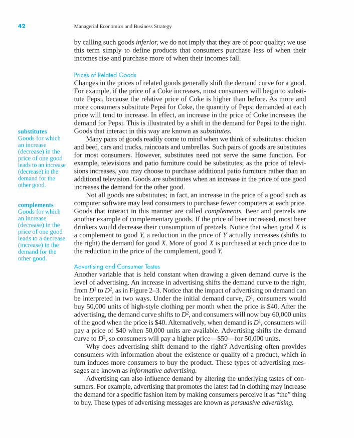
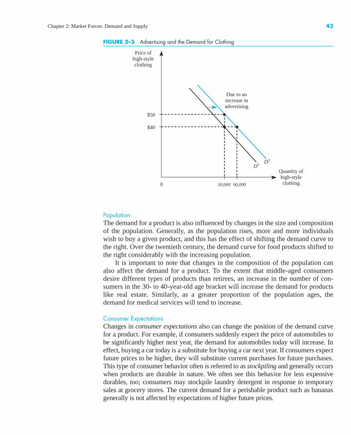
Advertising and Consumer TastesAnother variable that is held constant when drawing a given demand curve is thelevel of advertising. An increase in advertising shifts the demand curve to the right,from D1 to D2, as in Figure 2–3. Notice that the impact of advertising on demand canbe interpreted in two ways. Under the initial demand curve, D1, consumers wouldbuy 50,000 units of high-style clothing per month when the price is $40. After theadvertising, the demand curve shifts to D2, and consumers will now buy 60,000 unitsof the good when the price is $40. Alternatively, when demand is D1, consumers willpay a price of $40 when 50,000 units are available. Advertising shifts the demandcurve to D2, so consumers will pay a higher price—$50—for 50,000 units.

Why does advertising shift demand to the right? Advertising often providesconsumers with information about the existence or quality of a product, which inturn induces more consumers to buy the product. These types of advertising mes-sages are known as informative advertising.

Advertising can also influence demand by altering the underlying tastes of con-sumers. For example, advertising that promotes the latest fad in clothing may increasethe demand for a specific fashion item by making consumers perceive it as “the” thingto buy. These types of advertising messages are known as persuasive advertising.

substitutesGoods for whichan increase(decrease) in theprice of one goodleads to an increase(decrease) in thedemand for theother good.

complementsGoods for whichan increase(decrease) in theprice of one goodleads to a decrease(increase) in thedemand for theother good.

bay23224_ch02_037-076.qxd 12/14/12 10:04 AM Page 42

Confirming Pages

0

Price ofhigh-styleclothing

Quantity ofhigh-styleclothing50,000 60,000

$40

D1 D2

$50

Due to anincrease inadvertising

FIGURE 2–3 Advertising and the Demand for Clothing


PopulationThe demand for a product is also influenced by changes in the size and compositionof the population. Generally, as the population rises, more and more individualswish to buy a given product, and this has the effect of shifting the demand curve tothe right. Over the twentieth century, the demand curve for food products shifted tothe right considerably with the increasing population.

It is important to note that changes in the composition of the population canalso affect the demand for a product. To the extent that middle-aged consumersdesire different types of products than retirees, an increase in the number of con-sumers in the 30- to 40-year-old age bracket will increase the demand for productslike real estate. Similarly, as a greater proportion of the population ages, thedemand for medical services will tend to increase.

Consumer ExpectationsChanges in consumer expectations also can change the position of the demand curvefor a product. For example, if consumers suddenly expect the price of automobiles tobe significantly higher next year, the demand for automobiles today will increase. Ineffect, buying a car today is a substitute for buying a car next year. If consumers expectfuture prices to be higher, they will substitute current purchases for future purchases.This type of consumer behavior often is referred to as stockpiling and generally occurswhen products are durable in nature. We often see this behavior for less expensivedurables, too; consumers may stockpile laundry detergent in response to temporarysales at grocery stores. The current demand for a perishable product such as bananasgenerally is not affected by expectations of higher future prices.

bay23224_ch02_037-076.qxd 12/14/12 10:04 AM Page 43

Confirming Pages


demand functionA function thatdescribes howmuch of a goodwill be purchasedat alternativeprices of that goodand related goods,alternative incomelevels, andalternative valuesof other variablesaffecting demand.

Other FactorsIn concluding our list of demand shifters, we simply note that any variable thataffects the willingness or ability of consumers to purchase a particular good is apotential demand shifter. Health scares affect the demand for cigarettes. The birthof a baby affects the demand for diapers.

The Demand Function

By now you should understand the factors that affect demand and how to usegraphs to illustrate those influences. The final step in our analysis of the demandside of the market is to show that all the factors that influence demand may be sum-marized in what economists refer to as a demand function.

The demand function for good X describes how much X will be purchased atalternative prices of X and related goods, alternative levels of income, and alterna-tive values of other variables that affect demand. Formally, let represent thequantity demanded of good X, Px the price of good X, Py the price of a related good,M income, and H the value of any other variable that affects demand, such as thelevel of advertising, the size of the population, or consumer expectations. Then thedemand function for good X may be written as

Thus, the demand function explicitly recognizes that the quantity of a goodconsumed depends on its price and on demand shifters. Different products willhave demand functions of different forms. One very simple but useful form is thelinear representation of the demand function: Demand is linear if is a linearfunction of prices, income, and other variables that influence demand. The follow-ing equation is an example of a linear demand function:

The ais are fixed numbers that the firm’s research department or an economic con-sultant typically provides to the manager. (Chapter 3 provides an overview of thestatistical techniques used to obtain these numbers.)

By the law of demand, an increase in leads to a decrease in the quantitydemanded of good X. This means that ax � 0. The sign of ay will be positive or neg-ative depending on whether goods X and Y are substitutes or complements. If ay isa positive number, an increase in the price of good Y will lead to an increase in theconsumption of good X; therefore, good X is a substitute for good Y. If ay is a nega-tive number, an increase in the price of good Y will lead to a decrease in the con-sumption of good X; hence, good X is a complement to good Y. The sign of aM alsocan be positive or negative depending on whether X is a normal or an inferior good.If aM is a positive number, an increase in income (M) will lead to an increase in theconsumption of good X, and good X is a normal good. If aM is a negative number,an increase in income will lead to a decrease in the consumption of good X, andgood X is an inferior good.

Px

Qxd � a0 � axPx � ayPy � aMM � aHH

Qxd

Qxd � f (Px , Py , M, H)

Qxd

linear demandfunctionA representation ofthe demandfunction in whichthe demand for agiven good is alinear function ofprices, income lev-els, and other vari-ables influencingdemand.

bay23224_ch02_037-076.qxd 12/14/12 10:04 AM Page 44

Confirming Pages


Demonstration Problem 2–1

An economic consultant for X Corp. recently provided the firm’s marketing manager withthis estimate of the demand function for the firm’s product:

where represents the amount consumed of good X, Px is the price of good X, is the priceof good Y, M is income, and Ax represents the amount of advertising spent on good X.Suppose good X sells for $200 per unit, good Y sells for $15 per unit, the company utilizes2,000 units of advertising, and consumer income is $10,000. How much of good X do con-sumers purchase? Are goods X and Y substitutes or complements? Is good X a normal or aninferior good?

Answer:To find out how much of good X consumers will purchase, we substitute the given values ofprices, income, and advertising into the linear demand equation to get

Adding up the numbers, we find that the total consumption of X is 5,460 units. Sincethe coefficient of Py in the demand equation is 4 � 0, we know that a $1 increase in the priceof good Y will increase the consumption of good X by 4 units. Thus, goods X and Y are sub-stitutes. Since the coefficient of M in the demand equation is �1 � 0, we know that a $1increase in income will decrease the consumption of good X by 1 unit. Thus, good X is aninferior good.

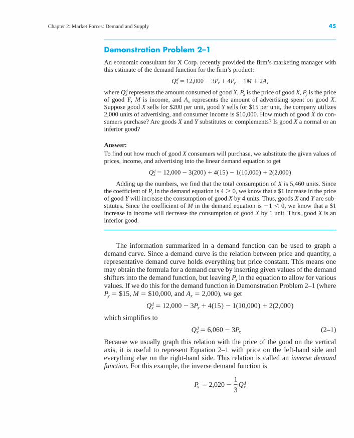
The information summarized in a demand function can be used to graph ademand curve. Since a demand curve is the relation between price and quantity, arepresentative demand curve holds everything but price constant. This means onemay obtain the formula for a demand curve by inserting given values of the demandshifters into the demand function, but leaving Px in the equation to allow for variousvalues. If we do this for the demand function in Demonstration Problem 2–1 (wherePy � $15, M � $10,000, and Ax � 2,000), we get

which simplifies to

(2–1)

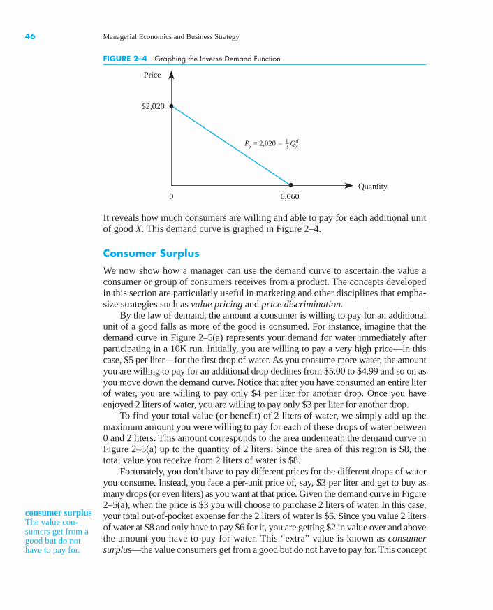
Because we usually graph this relation with the price of the good on the verticalaxis, it is useful to represent Equation 2–1 with price on the left-hand side andeverything else on the right-hand side. This relation is called an inverse demandfunction. For this example, the inverse demand function is

Px � 2,020 � 1

3Qx

d

Qxd � 6,060 � 3Px

Qxd � 12,000 � 3Px � 4(15) � 1(10,000) � 2(2,000)

Qxd � 12,000 � 3(200) � 4(15) � 1(10,000) � 2(2,000)

PyQxd

Qxd � 12,000 � 3Px � 4Py � 1M � 2Ax

bay23224_ch02_037-076.qxd 12/14/12 10:04 AM Page 45

Confirming Pages

0

Price

Quantity

Px = 2,020 – Qx

d

6,060

$2,020

1 3

FIGURE 2–4 Graphing the Inverse Demand Function


It reveals how much consumers are willing and able to pay for each additional unitof good X. This demand curve is graphed in Figure 2–4.

Consumer Surplus

We now show how a manager can use the demand curve to ascertain the value aconsumer or group of consumers receives from a product. The concepts developedin this section are particularly useful in marketing and other disciplines that empha-size strategies such as value pricing and price discrimination.

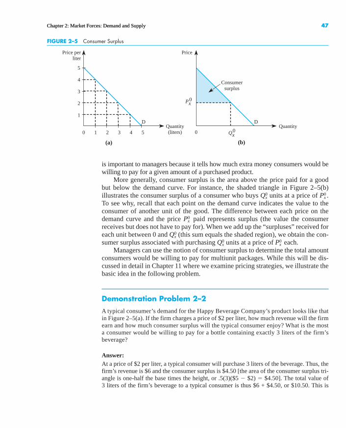
By the law of demand, the amount a consumer is willing to pay for an additionalunit of a good falls as more of the good is consumed. For instance, imagine that thedemand curve in Figure 2–5(a) represents your demand for water immediately afterparticipating in a 10K run. Initially, you are willing to pay a very high price—in thiscase, $5 per liter—for the first drop of water. As you consume more water, the amountyou are willing to pay for an additional drop declines from $5.00 to $4.99 and so on asyou move down the demand curve. Notice that after you have consumed an entire literof water, you are willing to pay only $4 per liter for another drop. Once you haveenjoyed 2 liters of water, you are willing to pay only $3 per liter for another drop.

To find your total value (or benefit) of 2 liters of water, we simply add up themaximum amount you were willing to pay for each of these drops of water between0 and 2 liters. This amount corresponds to the area underneath the demand curve inFigure 2–5(a) up to the quantity of 2 liters. Since the area of this region is $8, thetotal value you receive from 2 liters of water is $8.

Fortunately, you don’t have to pay different prices for the different drops of wateryou consume. Instead, you face a per-unit price of, say, $3 per liter and get to buy asmany drops (or even liters) as you want at that price. Given the demand curve in Figure2–5(a), when the price is $3 you will choose to purchase 2 liters of water. In this case,your total out-of-pocket expense for the 2 liters of water is $6. Since you value 2 litersof water at $8 and only have to pay $6 for it, you are getting $2 in value over and abovethe amount you have to pay for water. This “extra” value is known as consumersurplus—the value consumers get from a good but do not have to pay for. This concept

consumer surplusThe value con-sumers get from agood but do nothave to pay for.

bay23224_ch02_037-076.qxd 12/14/12 10:04 AM Page 46

Confirming Pages

Price perliter

Quantity(liters)

QuantityD

1 2 3 4 5

1

0

2

3

4

5

0

Price

D

Px0

Consumersurplus

Q0x

FIGURE 2–5 Consumer Surplus

(a) (b)


is important to managers because it tells how much extra money consumers would bewilling to pay for a given amount of a purchased product.

More generally, consumer surplus is the area above the price paid for a goodbut below the demand curve. For instance, the shaded triangle in Figure 2–5(b)illustrates the consumer surplus of a consumer who buys units at a price of .To see why, recall that each point on the demand curve indicates the value to theconsumer of another unit of the good. The difference between each price on thedemand curve and the price paid represents surplus (the value the consumerreceives but does not have to pay for). When we add up the “surpluses” received foreach unit between 0 and (this sum equals the shaded region), we obtain the con-sumer surplus associated with purchasing units at a price of each.

Managers can use the notion of consumer surplus to determine the total amountconsumers would be willing to pay for multiunit packages. While this will be dis-cussed in detail in Chapter 11 where we examine pricing strategies, we illustrate thebasic idea in the following problem.


A typical consumer’s demand for the Happy Beverage Company’s product looks like thatin Figure 2–5(a). If the firm charges a price of $2 per liter, how much revenue will the firmearn and how much consumer surplus will the typical consumer enjoy? What is the mosta consumer would be willing to pay for a bottle containing exactly 3 liters of the firm’sbeverage?

Answer:At a price of $2 per liter, a typical consumer will purchase 3 liters of the beverage. Thus, thefirm’s revenue is $6 and the consumer surplus is $4.50 [the area of the consumer surplus tri-angle is one-half the base times the height, or .5(3)($5 � $2) � $4.50]. The total value of 3 liters of the firm’s beverage to a typical consumer is thus $6 + $4.50, or $10.50. This is

Px0Qx

0Qx

0

Px0

Px0Qx

0

bay23224_ch02_037-076.qxd 12/14/12 10:04 AM Page 47

Confirming Pages

0

A

B

Price

Quantity

S2

S0

S1

Increase insupply

Decrease in supply

FIGURE 2–6 Changes in Supply


market supplycurveA curve indicatingthe total quantityof a good that allproducers in acompetitive marketwould produce ateach price, holdinginput prices, tech-nology, and othervariables affectingsupply constant.

change inquantity suppliedChanges in theprice of a goodlead to a changein the quantitysupplied of thatgood. This corre-sponds to amovement along agiven supplycurve.

also the maximum amount a consumer would be willing to pay for a bottle containingexactly 3 liters of the firm’s beverage. Expressed differently, if the firm sold the product in3-liter bottles rather than in smaller units, it could sell each bottle for $10.50 to earn higherrevenues and extract all consumer surplus.

SUPPLY

In the previous section we focused on demand, which represents half of the forcesthat determine the price in a market. The other determinant is market supply. In acompetitive market there are many producers, each producing a similar product. Themarket supply curve summarizes the total quantity all producers are willing and ableto produce at alternative prices, holding other factors that affect supply constant.

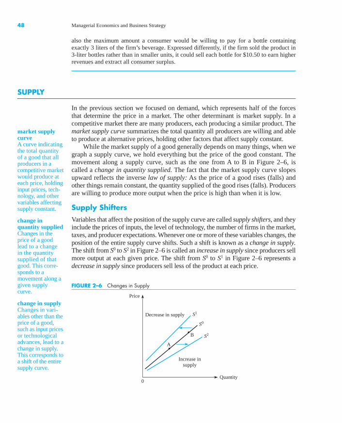
While the market supply of a good generally depends on many things, when wegraph a supply curve, we hold everything but the price of the good constant. Themovement along a supply curve, such as the one from A to B in Figure 2–6, iscalled a change in quantity supplied. The fact that the market supply curve slopesupward reflects the inverse law of supply: As the price of a good rises (falls) andother things remain constant, the quantity supplied of the good rises (falls). Producersare willing to produce more output when the price is high than when it is low.

Supply Shifters

Variables that affect the position of the supply curve are called supply shifters, and theyinclude the prices of inputs, the level of technology, the number of firms in the market,taxes, and producer expectations. Whenever one or more of these variables changes, theposition of the entire supply curve shifts. Such a shift is known as a change in supply.The shift from S0 to S2 in Figure 2–6 is called an increase in supply since producers sellmore output at each given price. The shift from S0 to S1 in Figure 2–6 represents adecrease in supply since producers sell less of the product at each price.

change in supplyChanges in vari-ables other than theprice of a good,such as input pricesor technologicaladvances, lead to achange in supply.This corresponds toa shift of the entiresupply curve.

bay23224_ch02_037-076.qxd 12/14/12 10:04 AM Page 48

Confirming Pages


The Trade Act of 2002, NAFTA, and the Supply Curve

Over the past two decades, presidents from both politi-cal parties have signed trade agreements and laws thatinclude provisions designed to reduce the cost of pro-ducing goods at home and abroad. These cost reduc-tions translate into increases in the supply of goods andservices available to U.S. consumers.

The North American Free Trade Agreement(NAFTA) between the United States, Canada, and Mex-ico was signed into law by Bill Clinton and containedprovisions to eliminate or phase out tariffs and other bar-riers in industrial products (such as textiles and apparel)and agricultural products. NAFTA also included provi-sions designed to reduce barriers to investment in Mexi-can petrochemicals and financial service sectors.

The Trade Act of 2002 was enacted under GeorgeW. Bush and gives the President the ability to negoti-

ate additional international agreements (subject to anup-or-down vote by Congress).

During his campaign and early in his presidency,Barack Obama pledged to renegotiate NAFTA. How-ever, the deep recession during that time caused himto postpone that effort. Only time will tell whetherthe current and future administrations will continueon the course set by Presidents Clinton and Bush.

Sources: “NAFTA Renegotiation Must Wait, Obama Says,”Washington Post, February 20, 2009; Economic Report of the President, Washington, D.C.: U.S. Government PrintingOffice, February 2007, p. 60; Economic Report of thePresident, Washington, D.C.: U.S. Government PrintingOffice, February 2006, p. 153; Economic Report of thePresident, Washington, D.C.: U.S. Government PrintingOffice, February 1995, pp. 220–21.


Input PricesThe supply curve reveals how much producers are willing to produce at alternativeprices. As production costs change, the willingness of producers to produce outputat a given price changes. In particular, as the price of an input rises, producers arewilling to produce less output at each given price. This decrease in supply isdepicted as a leftward shift in the supply curve.

Technology or Government RegulationsTechnological changes and changes in government regulations also can affect theposition of the supply curve. Changes that make it possible to produce a given out-put at a lower cost, such as the ones highlighted in Inside Business 2–2, have theeffect of increasing supply. Conversely, natural disasters that destroy existing tech-nology and government regulations, such as emissions standards that have anadverse effect on businesses, shift the supply curve to the left.

Number of FirmsThe number of firms in an industry affects the position of the supply curve. As addi-tional firms enter an industry, more and more output is available at each given price.This is reflected by a rightward shift in the supply curve. Similarly, as firms leave anindustry, fewer units are sold at each price, and the supply decreases (shifts to the left).

Substitutes in ProductionMany firms have technologies that are readily adaptable to several different products.For example, automakers can convert a truck assembly plant into a car assembly

bay23224_ch02_037-076.qxd 12/14/12 10:04 AM Page 49

Confirming Pages

0

Priceof

gasoline

Quantityof

gasolineper week

S0 + t

t = per unit taxof 20¢

S0

t = 20¢

$1

$1.20t

FIGURE 2–7 A Per Unit (Excise) Tax

{


plant by altering its production facilities. When the price of cars rises, these firmscan convert some of their truck assembly lines to car assembly lines to increase thequantity of cars supplied. This has the effect of shifting the truck supply curve tothe left.

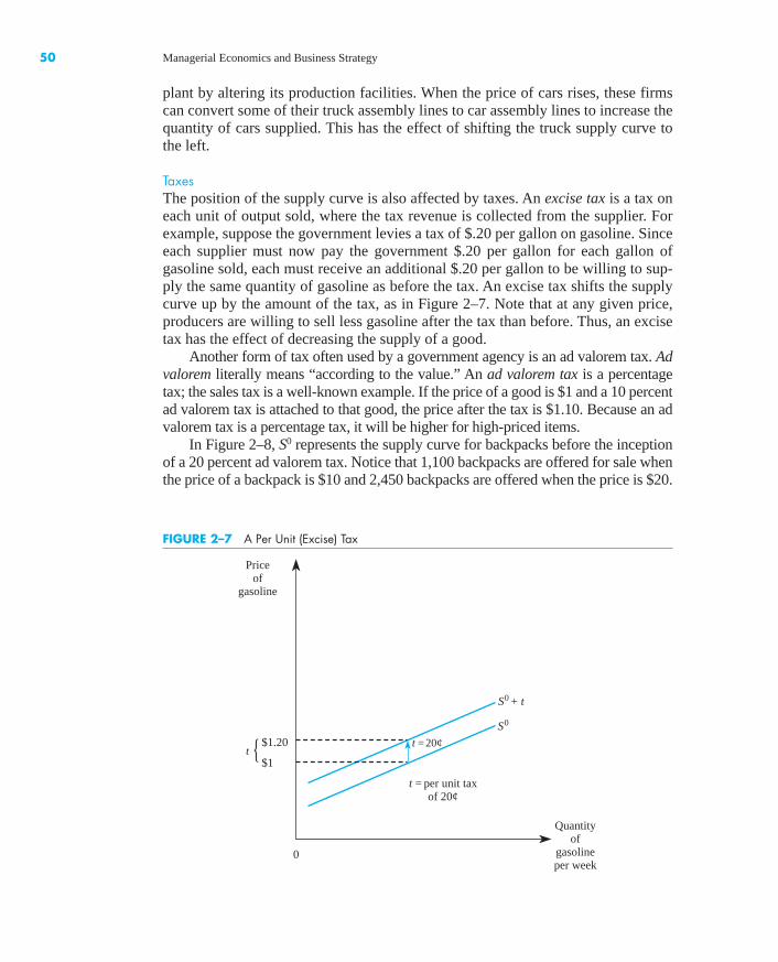
TaxesThe position of the supply curve is also affected by taxes. An excise tax is a tax oneach unit of output sold, where the tax revenue is collected from the supplier. Forexample, suppose the government levies a tax of $.20 per gallon on gasoline. Sinceeach supplier must now pay the government $.20 per gallon for each gallon ofgasoline sold, each must receive an additional $.20 per gallon to be willing to sup-ply the same quantity of gasoline as before the tax. An excise tax shifts the supplycurve up by the amount of the tax, as in Figure 2–7. Note that at any given price,producers are willing to sell less gasoline after the tax than before. Thus, an excisetax has the effect of decreasing the supply of a good.

Another form of tax often used by a government agency is an ad valorem tax. Advalorem literally means “according to the value.” An ad valorem tax is a percentagetax; the sales tax is a well-known example. If the price of a good is $1 and a 10 percentad valorem tax is attached to that good, the price after the tax is $1.10. Because an advalorem tax is a percentage tax, it will be higher for high-priced items.

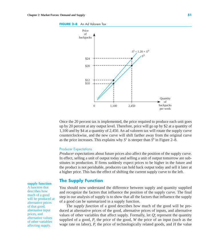
In Figure 2–8, S0 represents the supply curve for backpacks before the inceptionof a 20 percent ad valorem tax. Notice that 1,100 backpacks are offered for sale whenthe price of a backpack is $10 and 2,450 backpacks are offered when the price is $20.

bay23224_ch02_037-076.qxd 12/14/12 10:04 AM Page 50

Confirming Pages

0

Priceof

backpacks

Quantityof

backpacksper week

S1 = 1.20 × S0

S0

$10

$20

$24

$12

1,100 2,450

FIGURE 2–8 An Ad Valorem Tax


Once the 20 percent tax is implemented, the price required to produce each unit goesup by 20 percent at any output level. Therefore, price will go up by $2 at a quantity of1,100 and by $4 at a quantity of 2,450. An ad valorem tax will rotate the supply curvecounterclockwise, and the new curve will shift farther away from the original curveas the price increases. This explains why S1 is steeper than S0 in Figure 2–8.

Producer ExpectationsProducer expectations about future prices also affect the position of the supply curve.In effect, selling a unit of output today and selling a unit of output tomorrow are sub-stitutes in production. If firms suddenly expect prices to be higher in the future andthe product is not perishable, producers can hold back output today and sell it later ata higher price. This has the effect of shifting the current supply curve to the left.

The Supply Function

You should now understand the difference between supply and quantity suppliedand recognize the factors that influence the position of the supply curve. The finalstep in our analysis of supply is to show that all the factors that influence the supplyof a good can be summarized in a supply function.

The supply function of a good describes how much of the good will be pro-duced at alternative prices of the good, alternative prices of inputs, and alternativevalues of other variables that affect supply. Formally, let represent the quantitysupplied of a good, the price of the good, W the price of an input (such as thewage rate on labor), the price of technologically related goods, and H the valuePr

Px

Qxs

supply functionA function thatdescribes howmuch of a goodwill be produced atalternative pricesof that good,alternative inputprices, andalternative valuesof other variablesaffecting supply.

bay23224_ch02_037-076.qxd 12/14/12 10:04 AM Page 51

Confirming Pages


of some other variable that affects supply (such as the existing technology, the num-ber of firms in the market, taxes, or producer expectations). Then the supply func-tion for good X may be written as

Thus, the supply function explicitly recognizes that the quantity produced in amarket depends not only on the price of the good but also on all the factors that arepotential supply shifters. While there are many different functional forms for dif-ferent types of products, a particularly useful representation of a supply function is the linear relationship. Supply is linear if is a linear function of the variablesthat influence supply. The following equation is representative of a linear supplyfunction:

The coefficients (the bis) represent given numbers that have been estimated by thefirm’s research department or an economic consultant.


Your research department estimates that the supply function for television sets is given by

where Px is the price of TV sets, Pr represents the price of a computer monitor, and Pw is theprice of an input used to make television sets. Suppose TVs are sold for $400 per unit, com-puter monitors are sold for $100 per unit, and the price of an input is $2,000. How many tel-evision sets are produced?

Answer:To find out how many television sets are produced, we insert the given values of prices intothe supply function to get

Adding up the numbers, we find that the total quantity of television sets produced is 800.

The information summarized in a supply function can be used to graph a sup-ply curve. Since a supply curve is the relationship between price and quantity, arepresentative supply curve holds everything but price constant. This means onemay obtain the formula for a supply curve by inserting given values of the supplyshifters into the supply function, but leaving in the equation to allow for variousvalues. If we do this for the supply function in Demonstration Problem 2–3 (where

� $100 and � 2,000), we get

Qxs � 2,000 � 3Px � 4(100) � 1(2,000)

PwPr

Px

Qxs � 2,000 � 3(400) � 4(100) � 1(2,000)

Qxs � 2,000 � 3Px � 4Pr � Pw

Qxs � b0 � bxPx � brPr � bwW � bHH

Qxs

Qxs � f(Px, Pr, W, H)

linear supplyfunctionA representationof the supplyfunction in whichthe supply of agiven good is alinear function ofprices and othervariables affectingsupply.

bay23224_ch02_037-076.qxd 12/14/12 10:04 AM Page 52

Confirming Pages

0

Price

Quantity

$400

100 200 300 400 500 600

S

$400 3

700 800

A B

Producer surplus

900

Px = 400 + 1 3 3

C

Qxs

FIGURE 2–9 Producer Surplus


which simplifies to

(2–2)

Since we usually graph this relation with the price of the good on the vertical axis,it is useful to represent Equation 2–2 with price on the left-hand side and everythingelse on the right-hand side. This is known as an inverse supply function. For thisexample, the inverse supply function is

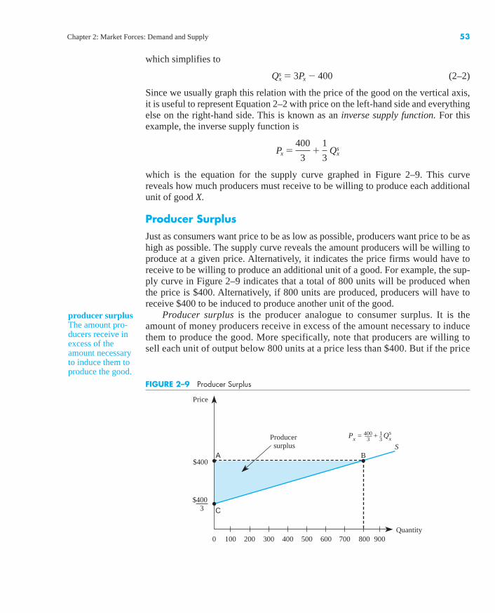
which is the equation for the supply curve graphed in Figure 2–9. This curvereveals how much producers must receive to be willing to produce each additionalunit of good X.

Producer Surplus

Just as consumers want price to be as low as possible, producers want price to be ashigh as possible. The supply curve reveals the amount producers will be willing toproduce at a given price. Alternatively, it indicates the price firms would have toreceive to be willing to produce an additional unit of a good. For example, the sup-ply curve in Figure 2–9 indicates that a total of 800 units will be produced whenthe price is $400. Alternatively, if 800 units are produced, producers will have toreceive $400 to be induced to produce another unit of the good.

Producer surplus is the producer analogue to consumer surplus. It is theamount of money producers receive in excess of the amount necessary to inducethem to produce the good. More specifically, note that producers are willing tosell each unit of output below 800 units at a price less than $400. But if the price

Px �400

3�

1

3 Qx

s

Qxs � 3Px � 400

producer surplusThe amount pro-ducers receive inexcess of theamount necessaryto induce them toproduce the good.

bay23224_ch02_037-076.qxd 12/14/12 10:04 AM Page 53

Confirming Pages

is $400, producers receive an amount equal to $400 for each unit of outputbelow 800, even though they would be willing to sell those individual units for alower price.

Geometrically, producer surplus is the area above the supply curve but belowthe market price of the good. Thus, the shaded area in Figure 2–9 represents the sur-plus producers receive by selling 800 units at a price of $400—an amount abovewhat would be required to produce each unit of the good. The shaded area, ABC, isthe producer surplus when the price is $400. Mathematically, this area is one-half of800 times $266.67, or $106,668.

Producer surplus can be a powerful tool for managers. For instance, suppose themanager of a major fast-food restaurant currently purchases 10,000 pounds ofground beef each week from a supplier at a price of $1.25 per pound. The producersurplus the meat supplier earns by selling 10,000 pounds at $1.25 per pound tells therestaurant manager the dollar amount that the supplier is receiving over and abovewhat it would be willing to accept for meat. In other words, the meat supplier’s pro-ducer surplus is the maximum amount the restaurant could save in meat costs by bar-gaining with the supplier over a package deal for 10,000 pounds of meat. Chapters 6and 10 will provide details about how managers can negotiate such a bargain.

MARKET EQUILIBRIUM

The equilibrium price in a competitive market is determined by the interactions of allbuyers and sellers in the market. The concepts of market supply and market demandmake this notion of interaction more precise: The price of a good in a competitive mar-ket is determined by the interaction of market supply and market demand for the good.

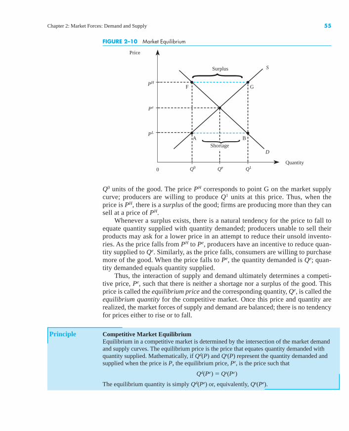
Since we will focus on the market for a single good, it is convenient to dropsubscripts at this point and let P denote the price of this good and Q the quantity ofthe good. Figure 2–10 depicts the market supply and demand curves for such agood. To see how the competitive price is determined, let the price of the good bePL. This price corresponds to point B on the market demand curve; consumers wishto purchase Q1 units of the good. Similarly, the price of PL corresponds to point Aon the market supply curve; producers are willing to produce only Q0 units at thisprice. Thus, when the price is PL, there is a shortage of the good; that is, there is notenough of the good to satisfy all consumers willing to purchase it at that price.

In situations where a shortage exists, there is a natural tendency for the price torise; consumers unable to buy the good may offer producers a higher price in anattempt to get the product. As the price rises from PL to Pe in Figure 2–10, produc-ers have an incentive to expand output from Q0 to Qe. Similarly, as the price rises,consumers are willing to purchase less of the good. When the price rises to Pe, thequantity demanded is Qe. At this price, just enough of the good is produced to sat-isfy all consumers willing and able to purchase at that price; quantity demandedequals quantity supplied.

Suppose the price is at a higher level—say, PH. This price corresponds topoint F on the market demand curve, indicating that consumers wish to purchase


bay23224_ch02_037-076.qxd 12/14/12 10:04 AM Page 54

Confirming Pages

0

Price

QuantityQ0

D

Qe Q1

A B

F G

S

PL

Pe

PH

Surplus

Shortage

FIGURE 2–10 Market Equilibrium

Q0 units of the good. The price PH corresponds to point G on the market supplycurve; producers are willing to produce Q1 units at this price. Thus, when theprice is PH, there is a surplus of the good; firms are producing more than they cansell at a price of PH.

Whenever a surplus exists, there is a natural tendency for the price to fall toequate quantity supplied with quantity demanded; producers unable to sell theirproducts may ask for a lower price in an attempt to reduce their unsold invento-ries. As the price falls from PH to Pe, producers have an incentive to reduce quan-tity supplied to Qe. Similarly, as the price falls, consumers are willing to purchasemore of the good. When the price falls to Pe, the quantity demanded is Qe; quan-tity demanded equals quantity supplied.

Thus, the interaction of supply and demand ultimately determines a competi-tive price, Pe, such that there is neither a shortage nor a surplus of the good. Thisprice is called the equilibrium price and the corresponding quantity, Qe, is called theequilibrium quantity for the competitive market. Once this price and quantity arerealized, the market forces of supply and demand are balanced; there is no tendencyfor prices either to rise or to fall.

Principle Competitive Market EquilibriumEquilibrium in a competitive market is determined by the intersection of the market demandand supply curves. The equilibrium price is the price that equates quantity demanded withquantity supplied. Mathematically, if Qd(P) and Qs(P) represent the quantity demanded andsupplied when the price is P, the equilibrium price, Pe, is the price such that

The equilibrium quantity is simply Qd(Pe) or, equivalently, Qs(Pe).

Qd(Pe) � Qs(Pe)

}

}


bay23224_ch02_037-076.qxd 12/14/12 10:04 AM Page 55

Confirming Pages


Unpopular Equilibrium Prices

For a recent college graduation, each graduating stu-dent was directed to pick up three free tickets any timebetween April 9 and April 20. After April 20, remainingtickets were given to those desiring additional tickets,on a first come, first served basis. Once the free ticketswere fully distributed, any trades between ticket hold-ers and ticket demanders were left to market forces—which led to a very unpopular equilibrium price.

With several concurrent events competing forstudents’ attention during this time, many students didnot claim their three free tickets by the deadline. Asgraduation approached, students who did not claimtheir tickets were willing to pay large sums of money

to purchase tickets for visiting family members andfriends. Since the demand for tickets was great andonly a limited number of tickets were available, somesellers were asking as much as $400 for a ticket!

Several students expressed outrage over the highprices. However, the high prices are merely a symp-tom of the high value many students placed on gradu-ation tickets coupled with the limited supply. Hadgraduating seniors without tickets better forecastedthis market outcome, they would have picked up theirfree tickets on time.

Source: “$400? Ticket Scalpers Cash in on IU Kelley’sCommencement,” The Herald-Times, May 3, 2012.



According to an article in China Daily, China recently accelerated its plan to privatize tensof thousands of state-owned firms. Imagine that you are an aide to a senator on the ForeignRelations Committee of the U.S. Senate, and you have been asked to help the committeedetermine the price and quantity that will prevail when competitive forces are allowed toequilibrate the market. The best estimates of the market demand and supply for the good (inU.S. dollar equivalent prices) are given by Qd � 10 � 2P and Qs � 2 + 2P, respectively.Determine the competitive equilibrium price and quantity.

Answer:Competitive equilibrium is determined by the intersection of the market demand and supplycurves. Mathematically, this simply means that Qd � Qs. Equating demand and supply yields

or

Solving this equation for P yields the equilibrium price, Pe � 2. To determine the equilib-rium quantity, we simply plug this price into either the demand or the supply function (since,in equilibrium, quantity supplied equals quantity demanded). For example, using the supplyfunction, we find that

PRICE RESTRICTIONS AND MARKET EQUILIBRIUM

The previous section showed how prices and quantities are determined in a free mar-ket. In some instances, government places limits on how much prices are allowed to

Qe � 2 � 2(2) � 6

8 � 4P

10 � 2P � 2 � 2P

bay23224_ch02_037-076.qxd 12/14/12 10:04 AM Page 56

Confirming Pages


rise or fall, and these restrictions can affect the market equilibrium. In this section, weexamine the impact of price ceilings and price floors on market allocations.

Price Ceilings

One basic implication of the economic doctrine of scarcity is that there are notenough goods to satisfy the desires of all consumers at a price of zero. As a conse-quence, some method must be used to determine who gets to consume goods andwho does not. People who do not get to consume goods are essentially discrimi-nated against. One way to determine who gets a good and who does not is to allo-cate the goods based on hair color: If you have red hair, you get the good; if youdon’t have red hair, you don’t get the good.

The price system uses price to determine who gets a good and who does not.The price system allocates goods to consumers who are willing and able to pay themost for the goods. If the competitive equilibrium price of a pair of jeans is $40,consumers willing and able to pay $40 will purchase the good; consumers unwill-ing or unable to pay that much for a pair of jeans will not buy the good.

It is important to keep in mind that it is not the price system that is “unfair” if onecannot afford to pay the market price for a good; rather, it is unfair that we live in aworld of scarcity. Any method of allocating goods will seem unfair to someone becausethere are not enough resources to satisfy everyone’s wants. For example, if jeans wereallocated to people on the basis of hair color instead of the price system, you wouldthink this allocation rule was unfair unless you were born with the “right” hair color.

Often individuals who are discriminated against by the price system attempt topersuade the government to intervene in the market by requiring producers to sellthe good at a lower price. This is only natural, for if we were unable to own a housebecause we had the wrong hair color, we most certainly would attempt to get thegovernment to pass a law allowing people with our hair color to own a house. Butthen there would be too few houses to go around, and some other means wouldhave to be used to allocate houses to people.

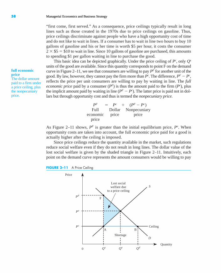
Suppose that, for whatever reason, the government views the equilibrium priceof Pe in Figure 2–11 as “too high” and passes a law prohibiting firms from chargingprices above Pc. Such a price is called a price ceiling.

Do not be confused by the fact that the price ceiling is below the initial equilib-rium price; the term ceiling refers to that price being the highest permissible pricein the market. It does not refer to a price set above the equilibrium price. In fact, ifa ceiling were imposed above the equilibrium price, it would be ineffective; theequilibrium price would be below the maximum legal price.

Given the regulated price of Pc, quantity demanded exceeds quantity suppliedby the distance from A to B in Figure 2–11; there is a shortage of Qd � Qs units. Thereason for the shortage is twofold. First, producers are willing to produce less at thelower price, so the available quantity is reduced from Qe to Qs. Second, consumerswish to purchase more at the lower price; thus, quantity demanded increases fromQe to Qd. The result is that there is not enough of the good to satisfy all consumerswilling and able to purchase it at the price ceiling.

How, then, are the goods to be allocated now that it is no longer legal to rationthem on the basis of price? In most instances, goods are rationed on the basis of

price ceilingThe maximumlegal price that canbe charged in amarket.

bay23224_ch02_037-076.qxd 12/14/12 10:04 AM Page 57

Confirming Pages

0

Price

QuantityQs

D

Qe Qd

A B

F

S

Pc

Pe

PF

Lost socialwelfare due

to a price ceiling

Ceiling

Shortage

FIGURE 2–11 A Price Ceiling


“first come, first served.” As a consequence, price ceilings typically result in longlines such as those created in the 1970s due to price ceilings on gasoline. Thus,price ceilings discriminate against people who have a high opportunity cost of timeand do not like to wait in lines. If a consumer has to wait in line two hours to buy 10gallons of gasoline and his or her time is worth $5 per hour, it costs the consumer 2 � $5 � $10 to wait in line. Since 10 gallons of gasoline are purchased, this amountsto spending $1 per gallon waiting in line to purchase the good.

This basic idea can be depicted graphically. Under the price ceiling of Pc, only Qs

units of the good are available. Since this quantity corresponds to point F on the demandcurve in Figure 2–11, we see that consumers are willing to pay PF for another unit of thegood. By law, however, they cannot pay the firm more than Pc. The difference, PF � Pc,reflects the price per unit consumers are willing to pay by waiting in line. The fulleconomic price paid by a consumer (PF) is thus the amount paid to the firm (Pc), plusthe implicit amount paid by waiting in line (PF � Pc). The latter price is paid not in dol-lars but through opportunity cost and thus is termed the nonpecuniary price.

As Figure 2–11 shows, PF is greater than the initial equilibrium price, Pe. Whenopportunity costs are taken into account, the full economic price paid for a good isactually higher after the ceiling is imposed.

Since price ceilings reduce the quantity available in the market, such regulationsreduce social welfare even if they do not result in long lines. The dollar value of thelost social welfare is given by the shaded triangle in Figure 2–11. Intuitively, eachpoint on the demand curve represents the amount consumers would be willing to pay

PF � Pc � (PF � Pc)Full Dollar Nonpecuniary

economic price priceprice

full economicpriceThe dollar amountpaid to a firm undera price ceiling, plusthe nonpecuniaryprice.

bay23224_ch02_037-076.qxd 12/14/12 10:04 AM Page 58

Confirming Pages


for an additional unit, while each point on the supply curve indicates the amount pro-ducers would have to receive to induce them to sell an additional unit. The verticaldifference between the demand and supply curves at each quantity therefore repre-sents the change in social welfare (consumer value less relevant production costs)associated with each incremental unit of output. Summing these vertical differencesfor all units between Qe and Qs yields the shaded triangle in Figure 2–11 and thus rep-resents the total dollar value of the lost social welfare due to a price ceiling. The tri-angle in Figure 2–11 is sometimes called “deadweight loss.”


Based on your answer to the Senate Foreign Relations Committee (Demonstration Problem2–4), one of the senators raises a concern that the free market price might be too high for thetypical Chinese citizen to pay. Accordingly, she asks you to explain what would happen ifthe Chinese government privatized the market, but then set a price ceiling at the Chineseequivalent of $1.50. How do you answer? Assume that the market demand and supplycurves (in U.S. dollar equivalent prices) are still given by

Qd � 10 � 2P and Qs � 2 � 2P

Answer:Since the price ceiling is below the equilibrium price of $2, a shortage will result. Morespecifically, when the price ceiling is $1.50, quantity demanded is

Qd � 10 � 2(1.50) � 7and quantity supplied is

Qs � 2 � 2(1.50) � 5

Thus, there is a shortage of 7 � 5 � 2 units.To determine the full economic price, we simply determine the maximum price con-

sumers are willing to pay for the five units produced. To do this, we first set quantity equalto 5 in the demand formula:

or

Next, we solve this equation for PF to obtain the full economic price, PF � $2.50.Thus, consumers pay a full economic price of $2.50 per unit; $1.50 of this price is in money,and $1 represents the nonpecuniary price of the good.

Based on the preceding analysis, one may wonder why the government wouldever impose price ceilings. One answer might be that politicians do not understandthe basics of supply and demand. This probably is not the answer, however.

The answer lies in who benefits from and who is harmed by ceilings. When linesdevelop due to a shortage caused by a price ceiling, people with high opportunity

2PF � 5

5 � 10 � 2PF

bay23224_ch02_037-076.qxd 12/14/12 10:04 AM Page 59

Confirming Pages



Price Ceilings and Price Floors around the Globe

Federal, state, and local authorities around the world areoften persuaded to enact laws that restrict the prices thatbusinesses can legally charge their customers. Manystates in the United States have usury laws—price ceil-ings on interest rates—that restrict the rate that banksand other lenders can legally charge their customers. In2005, Poland passed the Anti-Usury Act, which limitedthe consumer interest rate to quadruple the security rateof the National Bank of Poland; violators of the Act canface a fine or up to two years of imprisonment. Thailandallowed gasoline prices to be determined by marketforces during the 1990s, but its Commerce Ministryimposed a price ceiling in an attempt to hold down therapidly rising gasoline prices during the early 2000s.

All but five states in the United States have enactedminimum wage legislation—that is, a price floor on thehourly rate a business can legally pay its employees.These restrictions are in addition to the minimum wage setby the federal government, and as of 2012, state minimumwages were higher than the federal minimum wage in 18states. The effect of these minimum wages is similar to

that shown in Figure 2–12. However, since governmentsdo not hire workers who are unable to find employmentat the artificially high wage, the “surplus” of labor trans-lates into unemployment. Over a dozen Canadianprovinces also have enacted minimum wage laws. Inaddition, Ontario, British Columbia, and Quebec haveestablished floor prices (called “minimum retailprices”) on beer to keep prices artificially high in anattempt to discourage alcohol consumption and to pro-tect Canadian brewers from inexpensive U.S. brands.

Sources: “Oil Sales: Ceiling Set on Retail Margin,” TheNation, June 15, 2002; “An Oil Shock of Our OwnMaking,” The Nation, May 20, 2004; “Italian Usury Laws:Mercy Strain’d” The Economist, November 23, 2000;“Democrats Look to Keep Minimum Wage on Table,” TheWall Street Journal, June 20, 2006; “Beer Price War PunishesMom-and-Pop Shops,” The Gazette, November 4, 2005;“EU Lawmakers Pass Credit Directive,” Krakow Post, May 15, 2012; and United States Department of Labor,www.dol.gov/whd/ minwage/america.htm, accessed May 15, 2012.

costs are hurt, while people with low opportunity costs may actually benefit. Forexample, if you have nothing better to do than wait in line, you will benefit from thelower dollar price; your nonpecuniary price is close to zero. On the other hand, ifyou have a high opportunity cost of time because your time is valuable to you, youare made worse off by the ceiling. If a particular politician’s constituents tend tohave a lower than average opportunity cost, that politician naturally will attempt toinvoke a price ceiling.

Sometimes when shortages are created by a ceiling, goods are not allocated onthe basis of lines. Producers may discriminate against consumers on the basis ofother factors, including whether or not consumers are regular customers. Duringthe gasoline shortage of the 1970s, many gas stations sold gas only to customerswho regularly used the stations. In California during the late 1990s, price ceilingswere imposed on the fees that banks charged nondepositors for using their auto-matic teller machines (ATMs). The banks responded by refusing to let nondeposi-tors use their ATM machines. In other situations, such as ceilings on loan interestrates, banks may allocate money only to consumers who are relatively well-to-do.

The key point is that in the presence of a shortage created by a ceiling, man-agers must use some method other than price to allocate the goods. Depending onwhich method is used, some consumers will benefit and others will be worse off.

bay23224_ch02_037-076.qxd 12/14/12 10:04 AM Page 60

Confirming Pages

0

Price

QuantityQd

D

Qe Qs

F G

S

Pe

Pf

Cost of purchasing

excess supply

Surplus

Floor

FIGURE 2–12 A Price Floor


Price Floors

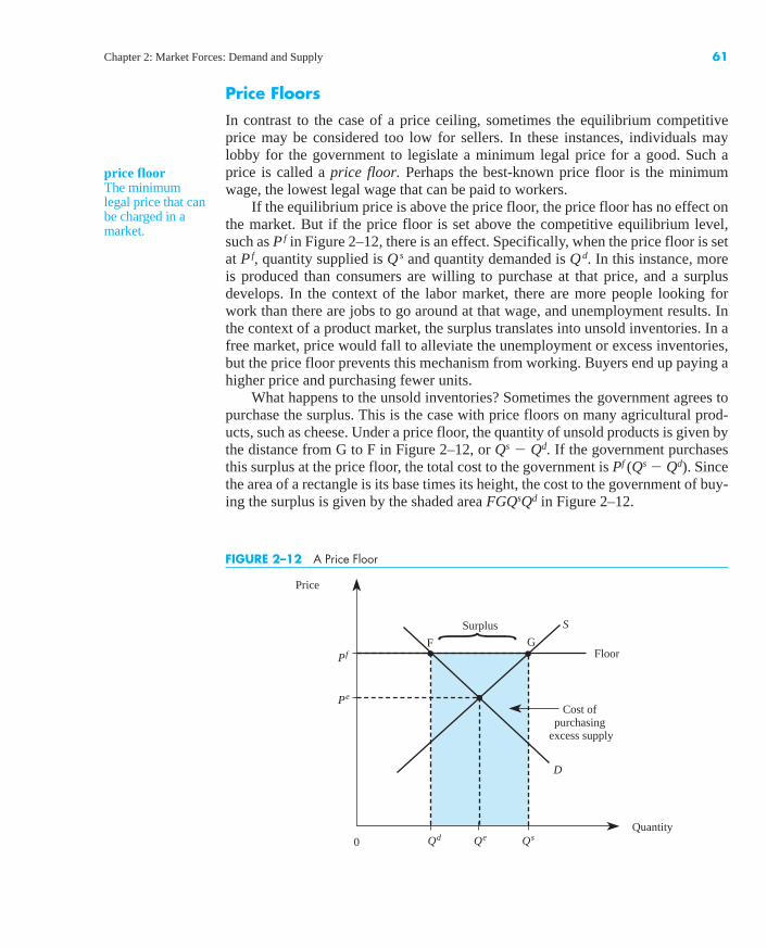
In contrast to the case of a price ceiling, sometimes the equilibrium competitiveprice may be considered too low for sellers. In these instances, individuals maylobby for the government to legislate a minimum legal price for a good. Such aprice is called a price floor. Perhaps the best-known price floor is the minimumwage, the lowest legal wage that can be paid to workers.

If the equilibrium price is above the price floor, the price floor has no effect onthe market. But if the price floor is set above the competitive equilibrium level,such as Pf in Figure 2–12, there is an effect. Specifically, when the price floor is setat Pf, quantity supplied is Qs and quantity demanded is Qd. In this instance, moreis produced than consumers are willing to purchase at that price, and a surplusdevelops. In the context of the labor market, there are more people looking forwork than there are jobs to go around at that wage, and unemployment results. Inthe context of a product market, the surplus translates into unsold inventories. In afree market, price would fall to alleviate the unemployment or excess inventories,but the price floor prevents this mechanism from working. Buyers end up paying ahigher price and purchasing fewer units.

What happens to the unsold inventories? Sometimes the government agrees topurchase the surplus. This is the case with price floors on many agricultural prod-ucts, such as cheese. Under a price floor, the quantity of unsold products is given bythe distance from G to F in Figure 2–12, or Qs � Qd. If the government purchasesthis surplus at the price floor, the total cost to the government is Pf (Qs � Qd). Sincethe area of a rectangle is its base times its height, the cost to the government of buy-ing the surplus is given by the shaded area FGQsQd in Figure 2–12.

price floorThe minimumlegal price that canbe charged in amarket.

}

bay23224_ch02_037-076.qxd 12/14/12 10:04 AM Page 61

Confirming Pages



One of the members of the Senate Foreign Relations Committee has studied your analysis ofChinese privatization (Demonstration Problems 2–4 and 2–5) but is worried that the free-market price might be too low to enable producers to earn a fair rate of return on theirinvestment. He asks you to explain what would happen if the Chinese government priva-tized the market, but agreed to purchase unsold units of the good at a floor price of $4. Whatdo you tell the senator? Assume that the market demand and supply curves (in U.S. dollarequivalent prices) are still given by

Qd � 10 � 2P and Qs � 2 � 2P

Answer:Since the price floor is above the equilibrium price of $2, the floor results in a surplus. Morespecifically, when the price is $4, quantity demanded is

Qd � 10 � 2(4) � 2

and quantity supplied is

Qs � 2 � 2(4) � 10

Thus, there is a surplus of 10 � 2 � 8 units. Consumers pay a higher price ($4), andproducers have unsold inventories of 8 units. However, the Chinese government must pur-chase the amount consumers are unwilling to purchase at the price of $4. Thus, the cost tothe Chinese government of buying the surplus of 8 units is $4 � 8 � $32.

COMPARATIVE STATICS

You now understand how equilibrium is determined in a competitive market andhow government policies such as price ceilings and price floors affect the market.Next, we show how managers can use supply and demand to analyze the impact ofchanges in market conditions on the competitive equilibrium price and quantity.The study of the movement from one equilibrium to another is known ascomparative static analysis. Throughout this analysis, we assume that no legalrestraints, such as price ceilings or floors, are in effect and that the price system isfree to work to allocate goods among consumers.

Changes in Demand

Suppose that The Wall Street Journal reports that consumer incomes are expected to riseby about 2.5 percent over the next year, and the number of individuals over 25 years ofage will reach an all-time high by the end of the year. We can use our supply anddemand apparatus to examine how these changes in market conditions will affect carrental agencies like Avis, Hertz, and National. It seems reasonable to presume that rentalcars are normal goods: Arise in consumer incomes will most likely increase the demandfor rental cars. The increased number of consumers aged 25 and older will also increasedemand, since at many locations those who rent cars must be at least 25 years old.

bay23224_ch02_037-076.qxd 12/14/12 10:04 AM Page 62

Confirming Pages

0

Price

Quantity(thousands

rented per day)

D0

100 104 108

B

S

$45

$49

D1

A

FIGURE 2–13 Effect of a Change in Demand for Rental Cars


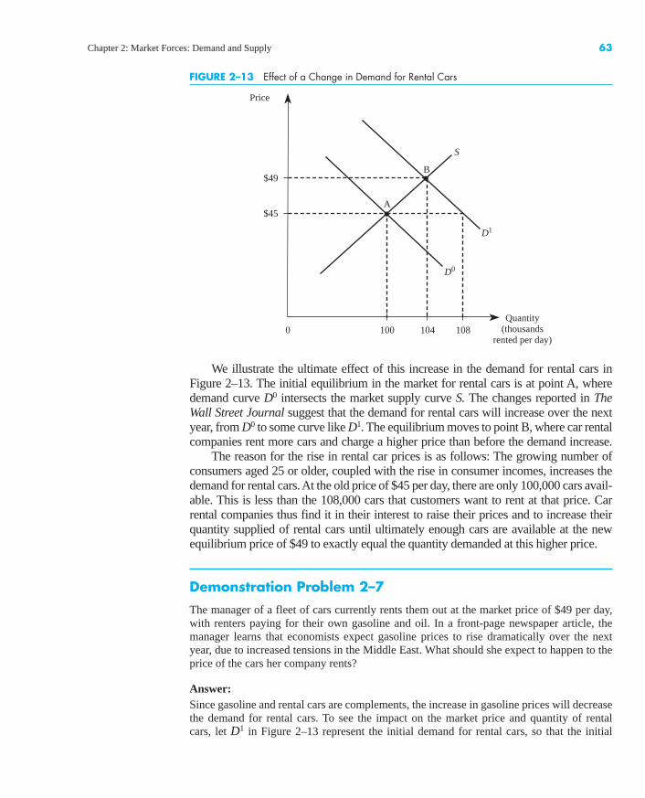
We illustrate the ultimate effect of this increase in the demand for rental cars inFigure 2–13. The initial equilibrium in the market for rental cars is at point A, wheredemand curve D0 intersects the market supply curve S. The changes reported in The Wall Street Journal suggest that the demand for rental cars will increase over the nextyear, from D0 to some curve like D1. The equilibrium moves to point B, where car rentalcompanies rent more cars and charge a higher price than before the demand increase.

The reason for the rise in rental car prices is as follows: The growing number ofconsumers aged 25 or older, coupled with the rise in consumer incomes, increases thedemand for rental cars. At the old price of $45 per day, there are only 100,000 cars avail-able. This is less than the 108,000 cars that customers want to rent at that price. Carrental companies thus find it in their interest to raise their prices and to increase theirquantity supplied of rental cars until ultimately enough cars are available at the newequilibrium price of $49 to exactly equal the quantity demanded at this higher price.


The manager of a fleet of cars currently rents them out at the market price of $49 per day,with renters paying for their own gasoline and oil. In a front-page newspaper article, themanager learns that economists expect gasoline prices to rise dramatically over the nextyear, due to increased tensions in the Middle East. What should she expect to happen to theprice of the cars her company rents?

Answer:Since gasoline and rental cars are complements, the increase in gasoline prices will decreasethe demand for rental cars. To see the impact on the market price and quantity of rental cars, let D1 in Figure 2–13 represent the initial demand for rental cars, so that the initial

bay23224_ch02_037-076.qxd 12/14/12 10:04 AM Page 63

Confirming Pages



Globalization and the Supply of Automobiles

In today’s global economy, the number of firms inthe market critically depends on the entry and exitdecisions of foreign firms. Recently, several Chineseautomakers—including the country's biggest domes-tic brand, Chery Automobile Co.—announced ambi-tious plans to expand abroad. Chery already exportsto 70 developing countries in Asia, the Middle East,and Latin America, and is eyeing further expansioninto more developed markets.

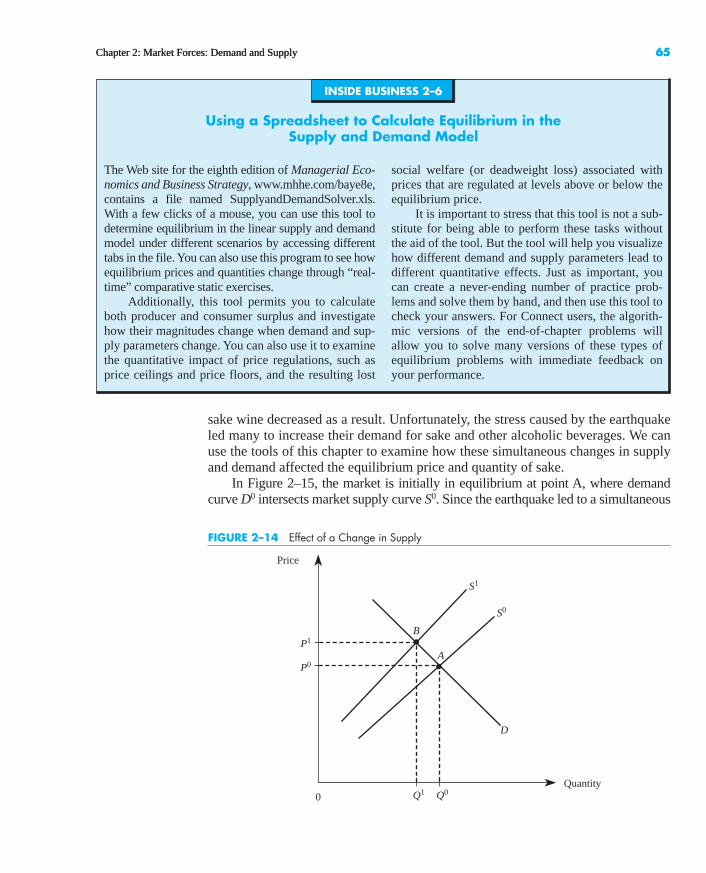
Entry by Chery and other Chinese manufacturersinto a developed market such as the U.S. automobilemarket would shift the supply curve to the right. Otherthings equal, this will negatively impact the bottomlines of firms that currently sell in these markets: Theincrease in supply will reduce the equilibrium prices ofautomobiles and the profits of existing U.S. automakers.Source: “Chinese Automakers Aim for Global Expansion,”Manufacturing.Net, April 23, 2010.

equilibrium is at point B. An increase in the price of gasoline will shift the demand curve forrental cars to the left (to D0), resulting in a new equilibrium at point A. Thus, she shouldexpect the price of rental cars to fall.

Changes in Supply

We can also use our supply and demand framework to predict how changes in one ormore supply shifters will affect the equilibrium price and quantity of goods or serv-ices. For instance, consider a bill before Congress that would require all employers,small and large alike, to provide health care to their workers. How would this billaffect the prices charged for goods at retailing outlets?

This health care mandate would increase the cost to retailers and other firms ofhiring workers. Many retailers rely on semiskilled workers who earn relatively lowwages, and the cost of providing health insurance to these workers is large relativeto their annual wage earnings. While firms might lower wages to some extent to offsetthe mandated health insurance costs paid, the net effect would be to raise the totalcost to the firm of hiring workers. These higher labor costs, in turn, would decreasethe supply of retail goods. The final result of the legislation would be to increase theprices charged by retailing outlets and to reduce the quantity of goods sold there.

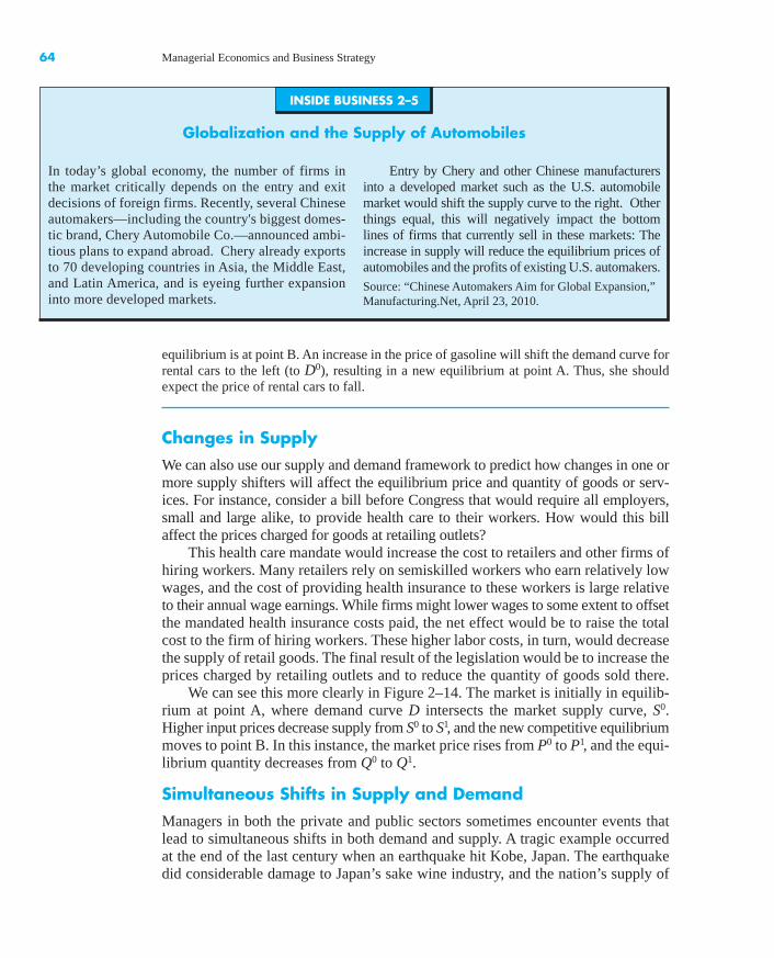
We can see this more clearly in Figure 2–14. The market is initially in equilib-rium at point A, where demand curve D intersects the market supply curve, S0.Higher input prices decrease supply from S0 to S1, and the new competitive equilibriummoves to point B. In this instance, the market price rises from P0 to P1, and the equi-librium quantity decreases from Q0 to Q1.

Simultaneous Shifts in Supply and Demand

Managers in both the private and public sectors sometimes encounter events thatlead to simultaneous shifts in both demand and supply. A tragic example occurredat the end of the last century when an earthquake hit Kobe, Japan. The earthquakedid considerable damage to Japan’s sake wine industry, and the nation’s supply of

bay23224_ch02_037-076.qxd 12/14/12 10:04 AM Page 64

Confirming Pages

0

Price

Quantity

D

Q1 Q0

S1

P0

P1B

S0

A

FIGURE 2–14 Effect of a Change in Supply


sake wine decreased as a result. Unfortunately, the stress caused by the earthquakeled many to increase their demand for sake and other alcoholic beverages. We canuse the tools of this chapter to examine how these simultaneous changes in supplyand demand affected the equilibrium price and quantity of sake.

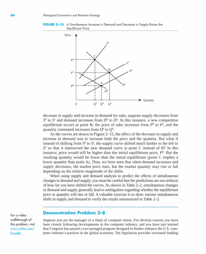
In Figure 2–15, the market is initially in equilibrium at point A, where demandcurve D0 intersects market supply curve S0. Since the earthquake led to a simultaneous


Using a Spreadsheet to Calculate Equilibrium in the Supply and Demand Model

The Web site for the eighth edition of Managerial Eco-nomics and Business Strategy, www.mhhe.com/baye8e,contains a file named SupplyandDemandSolver.xls.With a few clicks of a mouse, you can use this tool todetermine equilibrium in the linear supply and demandmodel under different scenarios by accessing differenttabs in the file. You can also use this program to see howequilibrium prices and quantities change through “real-time” comparative static exercises.

Additionally, this tool permits you to calculateboth producer and consumer surplus and investigatehow their magnitudes change when demand and sup-ply parameters change. You can also use it to examinethe quantitative impact of price regulations, such asprice ceilings and price floors, and the resulting lost

social welfare (or deadweight loss) associated withprices that are regulated at levels above or below theequilibrium price.

It is important to stress that this tool is not a sub-stitute for being able to perform these tasks withoutthe aid of the tool. But the tool will help you visualizehow different demand and supply parameters lead todifferent quantitative effects. Just as important, youcan create a never-ending number of practice prob-lems and solve them by hand, and then use this tool tocheck your answers. For Connect users, the algorith-mic versions of the end-of-chapter problems willallow you to solve many versions of these types ofequilibrium problems with immediate feedback onyour performance.

bay23224_ch02_037-076.qxd 12/14/12 10:04 AM Page 65

Confirming Pages

0

Price

QuantityQ2 Q0

S2

P1

P2C

S1

B

P0

Q1

A

S0

D1

D0

FIGURE 2–15 A Simultaneous Increase in Demand and Decrease in Supply Raises the Equilibrium Price


decrease in supply and increase in demand for sake, suppose supply decreases fromS0 to S1 and demand increases from D0 to D1. In this instance, a new competitiveequilibrium occurs at point B; the price of sake increases from P0 to P1, and thequantity consumed increases from Q0 to Q1.

As the curves are drawn in Figure 2–15, the effect of the decrease in supply andincrease in demand was to increase both the price and the quantity. But what ifinstead of shifting from S0 to S1, the supply curve shifted much farther to the left toS2 so that it intersected the new demand curve at point C instead of B? In thisinstance, price would still be higher than the initial equilibrium price, P0. But theresulting quantity would be lower than the initial equilibrium (point C implies alower quantity than point A). Thus, we have seen that when demand increases andsupply decreases, the market price rises, but the market quantity may rise or falldepending on the relative magnitude of the shifts.

When using supply and demand analysis to predict the effects of simultaneouschanges in demand and supply, you must be careful that the predictions are not artifactsof how far you have shifted the curves. As shown in Table 2–2, simultaneous changesin demand and supply generally lead to ambiguities regarding whether the equilibriumprice or quantity will rise or fall. A valuable exercise is to draw various simultaneousshifts in supply and demand to verify the results summarized in Table 2–2.


Suppose you are the manager of a chain of computer stores. For obvious reasons you havebeen closely following developments in the computer industry, and you have just learnedthat Congress has passed a two-pronged program designed to further enhance the U.S. com-puter industry’s position in the global economy. The legislation provides increased funding

For a video walkthrough of this problem, visitwww.mhhe.com/baye8e

bay23224_ch02_037-076.qxd 12/14/12 10:04 AM Page 66

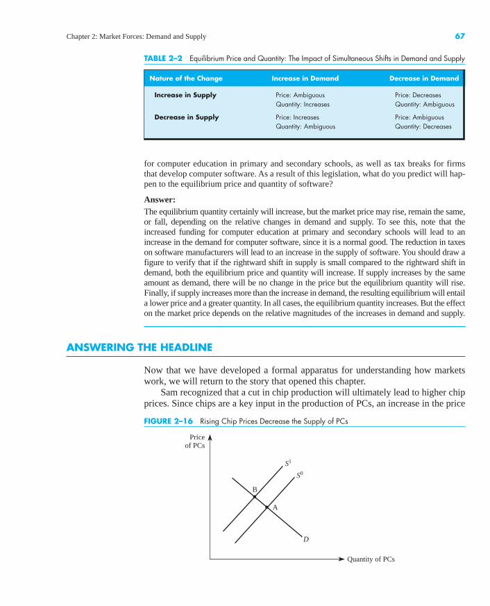
Confirming Pages

Priceof PCs

Quantity of PCs

S1

S0

B

A

D

FIGURE 2–16 Rising Chip Prices Decrease the Supply of PCs


for computer education in primary and secondary schools, as well as tax breaks for firmsthat develop computer software. As a result of this legislation, what do you predict will hap-pen to the equilibrium price and quantity of software?

Answer:The equilibrium quantity certainly will increase, but the market price may rise, remain the same,or fall, depending on the relative changes in demand and supply. To see this, note that theincreased funding for computer education at primary and secondary schools will lead to anincrease in the demand for computer software, since it is a normal good. The reduction in taxeson software manufacturers will lead to an increase in the supply of software. You should draw afigure to verify that if the rightward shift in supply is small compared to the rightward shift indemand, both the equilibrium price and quantity will increase. If supply increases by the sameamount as demand, there will be no change in the price but the equilibrium quantity will rise.Finally, if supply increases more than the increase in demand, the resulting equilibrium will entaila lower price and a greater quantity. In all cases, the equilibrium quantity increases. But the effecton the market price depends on the relative magnitudes of the increases in demand and supply.

ANSWERING THE HEADLINE

Now that we have developed a formal apparatus for understanding how marketswork, we will return to the story that opened this chapter.

Sam recognized that a cut in chip production will ultimately lead to higher chipprices. Since chips are a key input in the production of PCs, an increase in the price

TABLE 2–2 Equilibrium Price and Quantity: The Impact of Simultaneous Shifts in Demand and Supply

Nature of the Change Increase in Demand Decrease in Demand

Increase in Supply Price: Ambiguous Price: DecreasesQuantity: Increases Quantity: Ambiguous

Decrease in Supply Price: Increases Price: AmbiguousQuantity: Ambiguous Quantity: Decreases

bay23224_ch02_037-076.qxd 12/14/12 10:04 AM Page 67

Confirming Pages


ad valorem taxchange in demandchange in quantity demandedchange in quantity suppliedchange in supplycomparative static analysiscomplementsconsumer expectationsconsumer surplusdecrease in demanddecrease in supplydemanddemand functiondemand shiftersequilibrium priceequilibrium quantityexcise taxfull economic priceincrease in demandincrease in supplyinferior goodinformative advertising

inverse demand functioninverse supply functionlaw of demandlaw of supplylinear demand functionlinear supply functionmarket demand curvemarket supply curvenonpecuniary pricenormal goodpersuasive advertisingprice ceilingprice floorproducer expectationsproducer surplusshortagestockpilingsubstitutessupplysupply functionsupply shifterssurplus

of chips would in turn lead to a decrease in the market supply of PCs, as indicated bythe change in supply from S0 to S1 in Figure 2–16. Notice that total quantity of PCssold in the market falls as the equilibrium moves from point A to point B. In light ofthis anticipated decline in PC sales, Sam and Jane discussed the wisdom of goingahead with their plan to double PC Solutions’ workforce at this time.

SUMMARY

This chapter provided an overview of supply and demand and the interaction ofthese forces. We covered applications of demand, supply, price ceilings, pricefloors, and comparative statics. By reading this chapter and working through thedemonstration problems presented, you should have a basic understanding of howto analyze the workings of a competitive market.

The model of supply and demand is just a starting point for this book. Through-out the remainder of the book, we assume you have a thorough understanding of theconcepts presented in this chapter. In the next chapter, we will present the conceptsof elasticity and show how to use them in making managerial decisions. We will alsopresent some additional quantitative tools to help managers make better decisions.

KEY TERMS AND CONCEPTS

bay23224_ch02_037-076.qxd 12/14/12 10:04 AM Page 68

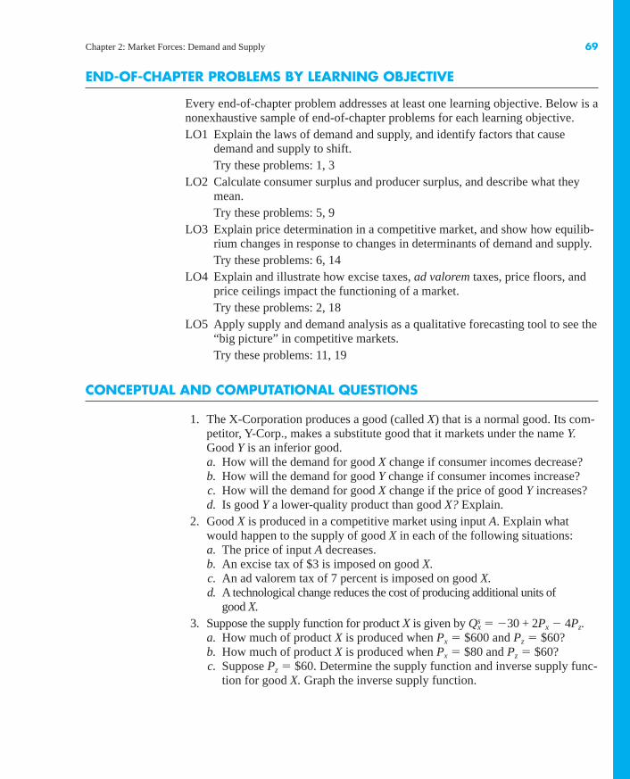
Confirming Pages


END-OF-CHAPTER PROBLEMS BY LEARNING OBJECTIVE

Every end-of-chapter problem addresses at least one learning objective. Below is anonexhaustive sample of end-of-chapter problems for each learning objective.LO1 Explain the laws of demand and supply, and identify factors that cause

demand and supply to shift.Try these problems: 1, 3

LO2 Calculate consumer surplus and producer surplus, and describe what theymean.Try these problems: 5, 9

LO3 Explain price determination in a competitive market, and show how equilib-rium changes in response to changes in determinants of demand and supply.Try these problems: 6, 14

LO4 Explain and illustrate how excise taxes, ad valorem taxes, price floors, andprice ceilings impact the functioning of a market.Try these problems: 2, 18

LO5 Apply supply and demand analysis as a qualitative forecasting tool to see the“big picture” in competitive markets.Try these problems: 11, 19

CONCEPTUAL AND COMPUTATIONAL QUESTIONS

1. The X-Corporation produces a good (called X) that is a normal good. Its com-petitor, Y-Corp., makes a substitute good that it markets under the name Y.Good Y is an inferior good.a. How will the demand for good X change if consumer incomes decrease?b. How will the demand for good Y change if consumer incomes increase?c. How will the demand for good X change if the price of good Y increases?d. Is good Y a lower-quality product than good X? Explain.

2. Good X is produced in a competitive market using input A. Explain whatwould happen to the supply of good X in each of the following situations:a. The price of input A decreases.b. An excise tax of $3 is imposed on good X.c. An ad valorem tax of 7 percent is imposed on good X.d. A technological change reduces the cost of producing additional units of

good X.3. Suppose the supply function for product X is given by � �30 + 2Px � 4Pz.

a. How much of product X is produced when Px � $600 and Pz � $60?b. How much of product X is produced when Px � $80 and Pz � $60?c. Suppose Pz � $60. Determine the supply function and inverse supply func-

tion for good X. Graph the inverse supply function.

Qxs

bay23224_ch02_037-076.qxd 12/14/12 10:04 AM Page 69

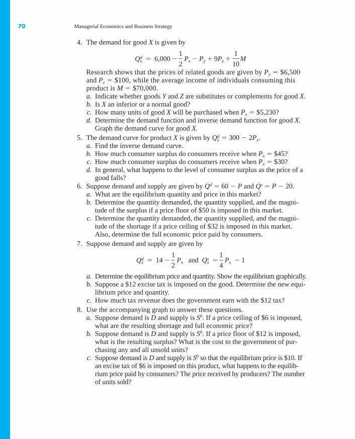
Confirming Pages


4. The demand for good X is given by

Research shows that the prices of related goods are given by Py � $6,500and Pz � $100, while the average income of individuals consuming thisproduct is M � $70,000.a. Indicate whether goods Y and Z are substitutes or complements for good X.b. Is X an inferior or a normal good?c. How many units of good X will be purchased when Px � $5,230?d. Determine the demand function and inverse demand function for good X.

Graph the demand curve for good X.5. The demand curve for product X is given by � 300 � 2Px.

a. Find the inverse demand curve.b. How much consumer surplus do consumers receive when Px � $45?c. How much consumer surplus do consumers receive when Px � $30?d. In general, what happens to the level of consumer surplus as the price of a

good falls?6. Suppose demand and supply are given by Qd � 60 � P and Qs � P � 20.

a. What are the equilibrium quantity and price in this market?b. Determine the quantity demanded, the quantity supplied, and the magni-

tude of the surplus if a price floor of $50 is imposed in this market.c. Determine the quantity demanded, the quantity supplied, and the magni-

tude of the shortage if a price ceiling of $32 is imposed in this market.Also, determine the full economic price paid by consumers.

7. Suppose demand and supply are given by

a. Determine the equilibrium price and quantity. Show the equilibrium graphically.b. Suppose a $12 excise tax is imposed on the good. Determine the new equi-

librium price and quantity.c. How much tax revenue does the government earn with the $12 tax?

8. Use the accompanying graph to answer these questions.a. Suppose demand is D and supply is S0. If a price ceiling of $6 is imposed,

what are the resulting shortage and full economic price?b. Suppose demand is D and supply is S0. If a price floor of $12 is imposed,

what is the resulting surplus? What is the cost to the government of pur-chasing any and all unsold units?

c. Suppose demand is D and supply is S0 so that the equilibrium price is $10. Ifan excise tax of $6 is imposed on this product, what happens to the equilib-rium price paid by consumers? The price received by producers? The numberof units sold?

Qxd � 14 �

1

2 Px and Qx

s �1

4 Px � 1

Qxd

Qxd � 6,000 �

1

2 Px � Py � 9Pz �

1

10 M

bay23224_ch02_037-076.qxd 12/14/12 10:04 AM Page 70

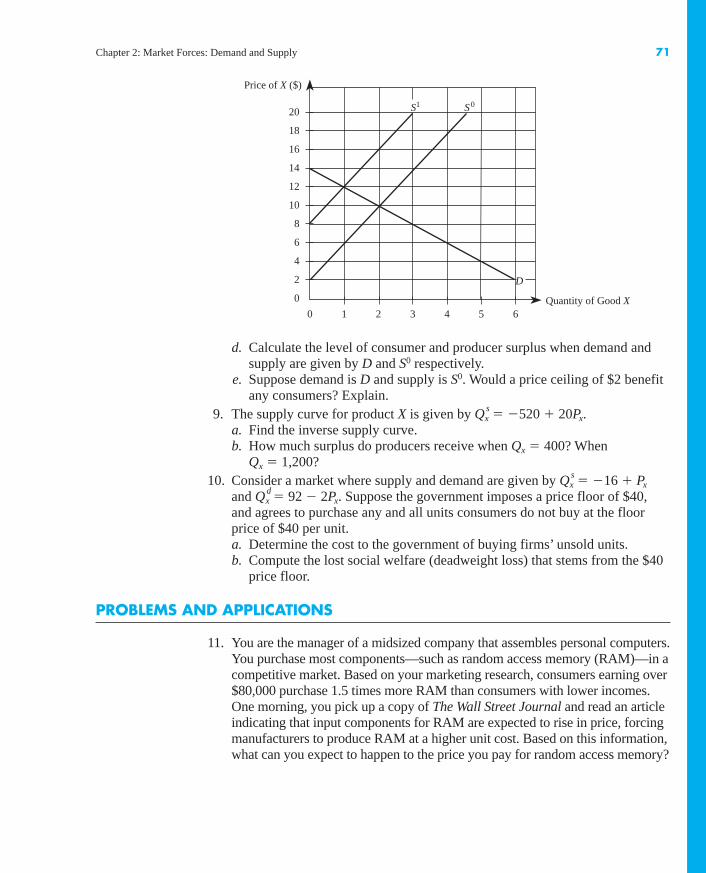
Confirming Pages

0 1 2 3 4 5 6

Price of X ($)

Quantity of Good X

20

18

16

14

12

10

8

6

4

2

0

S1 S0

D


d. Calculate the level of consumer and producer surplus when demand andsupply are given by D and S0 respectively.

e. Suppose demand is D and supply is S0. Would a price ceiling of $2 benefitany consumers? Explain.

9. The supply curve for product X is given by Qsx � �520 � 20Px.

a. Find the inverse supply curve.b. How much surplus do producers receive when Qx � 400? When

Qx � 1,200?10. Consider a market where supply and demand are given by Qs

x � �16 � Px

and Qdx � 92 � 2Px. Suppose the government imposes a price floor of $40,

and agrees to purchase any and all units consumers do not buy at the floorprice of $40 per unit.a. Determine the cost to the government of buying firms’ unsold units.b. Compute the lost social welfare (deadweight loss) that stems from the $40

price floor.

PROBLEMS AND APPLICATIONS

11. You are the manager of a midsized company that assembles personal computers.You purchase most components—such as random access memory (RAM)—in acompetitive market. Based on your marketing research, consumers earning over$80,000 purchase 1.5 times more RAM than consumers with lower incomes.One morning, you pick up a copy of The Wall Street Journal and read an articleindicating that input components for RAM are expected to rise in price, forcingmanufacturers to produce RAM at a higher unit cost. Based on this information,what can you expect to happen to the price you pay for random access memory?

bay23224_ch02_037-076.qxd 12/14/12 10:04 AM Page 71

Confirming Pages


Would your answer change if, in addition to this change in RAM input prices,the article indicated that consumer incomes are expected to fall over the nexttwo years as the economy dips into recession? Explain.

12. You are the manager of a firm that produces and markets a generic type of softdrink in a competitive market. In addition to the large number of generic productsin your market, you also compete against major brands such as Coca-Cola andPepsi. Suppose that, due to the successful lobbying efforts of sugar producers inthe United States, Congress is going to levy a $0.50 per pound tariff on allimported raw sugar—the primary input for your product. In addition, Coke andPepsi plan to launch an aggressive advertising campaign designed to persuadeconsumers that their branded products are superior to generic soft drinks. Howwill these events impact the equilibrium price and quantity of generic soft drinks?

13. Some have argued that higher cigarette prices do not deter smoking. Whilethere are many arguments both for and against this view, some find the follow-ing argument to be the most persuasive of all: “The laws of supply and demandindicate that higher prices are ineffective in reducing smoking. In particular,higher cigarette prices will reduce the demand for cigarettes. This reduction indemand will push the equilibrium price back down to its original level. Sincethe equilibrium price will remain unchanged, smokers will consume the samenumber of cigarettes.” Do you agree or disagree with this view? Explain.

14. You are the manager of an organization in America that distributes blood to hospitals in all 50 states and the District of Columbia. A recent report indicatesthat nearly 50 Americans contract HIV each year through blood transfusions.Although every pint of blood donated in the United States undergoes a batteryof nine different tests, existing screening methods can detect only the antibodiesproduced by the body’s immune system—not foreign agents in the blood. Sinceit takes weeks or even months for these antibodies to build up in the blood,newly infected HIV donors can pass along the virus through blood that haspassed existing screening tests. Happily, researchers have developed a series ofnew tests aimed at detecting and removing infections from donated blood beforeit is used in transfusions. The obvious benefit of these tests is the reduced inci-dence of infection through blood transfusions. The report indicates that the cur-rent price of decontaminated blood is $60 per pint. However, if the newscreening methods are adopted, the demand and supply for decontaminatedblood will change to Qd � 210 � 1.5P and Qs � 2.5P � 150. What price doyou expect to prevail if the new screening methods are adopted? How manyunits of blood will be used in the United States? What is the level of consumerand producer surplus? Illustrate your findings in a graph.

15. As a result of increased tensions in the Middle East, oil production is down by1.21 million barrels per day—a 5 percent reduction in the world’s supply ofcrude oil. Explain the likely impact of this event on the market for gasolineand the market for small cars.

bay23224_ch02_037-076.qxd 12/14/12 10:04 AM Page 72

Confirming Pages


16. You are an assistant to a senator who chairs an ad hoc committee on reformingtaxes on telecommunication services. Based on your research, AT&T has spentover $15 million on related paperwork and compliance costs. Moreover,depending on the locale, telecom taxes can amount to as much as 25 percent ofa consumer’s phone bill. These high tax rates on telecom services have becomequite controversial, due to the fact that the deregulation of the telecom industry has led to a highly competitive market. Your best estimatesindicate that, based on current tax rates, the monthly market demand fortelecommunication services is given by Qd � 300 � 4P and the market supply (including taxes) is Qs � 3P � 120 (both in millions), where P is themonthly price of telecommunication services. The senator is considering taxreform that would dramatically cut tax rates, leading to a supply function underthe new tax policy of Qs � 3.2P � 120. How much money per unit would atypical consumer save each month as a result of the proposed legislation?

17. G.R. Dry Foods Distributors specializes in the wholesale distribution of drygoods, such as rice and dry beans. The firm’s manager is concerned about anarticle he read in this morning’s Wall Street Journal indicating that theincomes of individuals in the lowest income bracket are expected to increaseby 10 percent over the next year. While the manager is pleased to see thisgroup of individuals doing well, he is concerned about the impact this willhave on G.R. Dry Foods. What do you think is likely to happen to the price ofthe products G.R. Dry Foods sells? Why?

18. From California to New York, legislative bodies across the United States areconsidering eliminating or reducing the surcharges that banks impose on non-customers who make $12 million in withdrawals from other banks’ATMmachines. On average, noncustomers earn a wage of $24 per hour and payATM fees of $3.00 per transaction. It is estimated that banks would be willingto maintain services for 5 million transactions at $1.25 per transaction, whilenoncustomers would attempt to conduct 19 million transactions at that price.Estimates suggest that, for every 1 million gap between the desired and avail-able transactions, a typical consumer will have to spend an extra minute trav-eling to another machine to withdraw cash. Based on this information, use agraph to carefully illustrate the impact of legislation that would place a $1.25cap on the fees banks can charge for noncustomer transactions.

19. Rapel Valley in Chile is renowned for its ability to produce high-quality wine at afraction of the cost of many other vineyards around the world. Rapel Valley pro-duces over 20 million bottles of wine annually, of which 5 million are exportedto the United States. Each bottle entering the United States is subjected to a $0.50per bottle excise tax, which generates about $2.5 million in tax revenues. StrongLa Niña weather patterns have caused unusually cold temperatures, devastatingmany of the wine producers in that region of Chile. How will La Niña affect theprice of Chilean wine? Assuming La Niña does not impact the California wine-producing region, how will La Niña impact the market for Californian wines?

bay23224_ch02_037-076.qxd 12/14/12 10:04 AM Page 73

Confirming Pages


20. Viking InterWorks is one of many manufacturers that supplies memory prod-ucts to original equipment manufacturers (OEMs) of desktop systems. TheCEO recently read an article in a trade publication that reported the projecteddemand for desktop systems to be Qd

desktop � 1,600 � 2Pdesktop + .6M (in mil-lions of units), where Pdesktop is the price of a desktop system and M is con-sumer income. The same article reported that the incomes of the desktopsystems’ primary consumer demographic would increase 4.2 percent this yearto $61,300 and that the selling price of a desktop would decrease to $980, bothof which the CEO viewed favorably for Viking. In a related article, the CEOread that the upcoming year’s projected demand for 512 MB desktop memorymodules is Qd

memory � 11,200 � 100Pmemory � 2Pdesktop (in thousands of units),where Pmemory is the market price for a 512 MB memory module and Pdesktop isthe selling price of a desktop system. The report also indicated that five new,small start-ups entered the 512 MB memory module market, bringing the totalnumber of competitors to 100 firms. Furthermore, suppose that Viking’s CEOcommissioned an industrywide study to examine the industry capacity for 512MB memory modules. The results indicate that when the industry is operatingat maximum efficiency, this competitive industry supplies modules accordingto the following function: QS

memory � 1,000 � 25Pmemory + N (in thousands),where Pmemory is the price of a 512 MB memory module and N is the number ofmemory module manufacturers in the market. Viking’s CEO provides you, theproduction manager, with the above information and requests a report contain-ing the market price for memory modules and the number of units to manufac-ture in the upcoming year based on the assumption that all firms producing 512MB modules supply an equal share to the market. How would your reportchange if the price of desktops were $1,080? What does this indicate about therelationship between memory modules and desktop systems?

21. Seventy-two percent of the members of the United Food and CommercialWorkers Local 655 voted to strike against Stop ’n Shop in the St. Louis area.In fear of similar union responses, two of Stop ’n Shop’s larger rivals in theSt. Louis market—Dierberg’s and Schnuck’s—decided to lock out theirunion employees. The actions of these supermarkets, not surprisingly, causedLocal 655 union members to picket and boycott each of the supermarkets’locations. While the manager of Mid Towne IGA—one of many smallercompeting grocers—viewed the strike as unfortunate for both sides, he wasquick to point out that the strike provided an opportunity for his store toincrease market share. To take advantage of the strike, the manager of MidTowne IGA increased newspaper advertising by pointing out that Mid Towneemployed Local 655 union members and that it operated under a differentcontract than “other” grocers in the area. Use a graph to describe theexpected impact of advertising on Mid Towne IGA (how the equilibriumprice and quantity change). Identify the type of advertising in which Mid

bay23224_ch02_037-076.qxd 12/14/12 10:04 AM Page 74

Confirming Pages


Towne IGA engaged. Do you believe the impact of advertising will be per-manent? Explain.

22. Florida, like several other states, has passed a law that prohibits “price gouging”immediately before, during, or after the declaration of a state of emergency. Pricegouging is defined as “ . . . selling necessary commodities such as food, gas, ice,oil, and lumber at a price that grossly exceeds the average selling price for the 30days prior to the emergency.” Many consumers attempt to stock up on emer-gency supplies, such as bottled water, immediately before and after a hurricaneor other natural disaster hits an area. Also, many supply shipments to retailers areinterrupted during a natural disaster. Assuming that the law is strictly enforced,what are the economic effects of the price gouging statute? Explain carefully.

23. In a recent speech, the governor of your state announced: “One of the biggestcauses of juvenile delinquency in this state is the high rate of unemploymentamong 16 to 19 year olds. The low wages offered by employers in the state havegiven fewer teenagers the incentive to find summer employment. Instead ofworking all summer, the way we used to, today’s teenagers slack off and causetrouble. To address this problem, I propose to raise the state’s minimum wage by$1.50 per hour. This will give teens the proper incentive to go out and find mean-ingful employment when they are not in school.” Evaluate the governor’s plan toreduce juvenile delinquency.

CONNECT EXERCISES

If your instructor has adopted Connect for the course and you are an active sub-scriber, you can practice with the questions presented above, along with many alter-native versions of these questions. Your instructor may also assign a subset of theseproblems and/or their alternative versions as a homework assignment through Con-nect, allowing for immediate feedback of grades and correct answers.

CASE-BASED EXERCISES

Your instructor may assign additional problem-solving exercises (called memos) thatrequire you to apply some of the tools you learned in this chapter to make a recommen-dation based on an actual business scenario. Some of these memos accompany the TimeWarner case (pages 561–597 of your textbook). Additional memos, as well as data thatmay be useful for your analysis, are available online at www.mhhe.com/baye8e.

SELECTED READINGS

Ault, Richard W.; Jackson, John D.; and Saba, Richard P., “The Effect of Long-Term Rent Con-trol on Tenant Mobility.” Journal of Urban Economics 35(2), March 1994, pp. 140–58.

bay23224_ch02_037-076.qxd 12/14/12 10:04 AM Page 75

Confirming Pages


Espana, Juan R., “Impact of the North American Free Trade Agreement (NAFTA) on U.S.–Mexican Trade and Investment Flows.” Business Economics 28(3), July 1993, pp. 41–47.

Friedman, Milton, Capitalism and Freedom. Chicago: University of Chicago Press, 1962.Katz, Lawrence F., and Murphy, Kevin M., “Changes in Relative Wages, 1963–1987:

Supply and Demand Factors.” Quarterly Journal of Economics 107(1), February 1992,pp. 35–78.

Olson, Josephine E., and Frieze, Irene Hanson, “Job Interruptions and Part-Time Work: TheirEffect on MBAs’ Income.” Industrial Relations 28(3), Fall 1989, pp. 373–86.

O’Neill, June, and Polachek, Solomon, “Why the Gender Gap in Wages Narrowed in the1980s.” Journal of Labor Economics 11(1), January 1993, pp. 205–28.

Simon, Herbert A., “Organizations and Markets.” Journal of Economic Perspectives 5(2),Spring 1991, pp. 25–44.

Smith, Vernon L., “An Experimental Study of Competitive Market Behavior.” Journal ofPolitical Economy 70(2), April 1962, pp. 111–39.

Williamson, Oliver, The Economic Institutions of Capitalism. New York: Free Press, 1985.

bay23224_ch02_037-076.qxd 12/14/12 10:04 AM Page 76

Documents

Market Forces: Demand and Supply - testbanklib.com · of the National Bank of Poland; ... The Web site for the eighth edition of Managerial Eco- ... 76 Managerial Economics and Business