Market Size and Pharmaceutical Innovation

Pierre Dubois∗, Olivier de Mouzon†, Fiona Scott-Morton‡, Paul Seabright§

This Version: March 2014¶

Abstract

This paper quantifies the relationship between market size and innovation in the pharmaceuticalindustry using improved, and newer, methods and data. We find positive significant elasticities ofinnovation to expected market size with a point estimate under our preferred specification of 0.23.This suggests that, on average, $2.5 billion is required in additional revenue to support the inventionof one new chemical entity. This magnitude is plausible given recent accounting estimates of thecost of innovation of 800 million to one billion per drug, and marginal costs of manufacture anddistribution near 50%. An elasticity below 1 is also a plausible implication of the hypothesis thatinnovation in pharmaceuticals is becoming more difficult over time, as costs of regulatory approvalrise and as the industry runs out of ”low-hanging fruit”.

Key words: Innovation, Market Size, Elasticity, Pharmaceuticals.

JEL codes: O31, L65, O34.

∗Toulouse School of Economics (GREMAQ, IDEI), pierre.dubois@tse-fr.eu†Toulouse School of Economics (GREMAQ, INRA), olivier.demouzon@tse-fr.eu‡Yale University, fiona.scottmorton@yale.edu§Toulouse School of Economics (GREMAQ, IDEI), paul.seabright@tse-fr.eu¶We thank Tamer Abdelgawad, Amber Batata, Bruno Jullien, Bernard Salanie and seminar participants at Toulouse,

PEPC Paris, Imperial College London for useful comments. The statements, findings, conclusions, views, and opinionscontained and expressed in this article are based in part on data obtained under license from the following IMS HealthIncorporated information service(s): MIDASTM (1997–2007), IMS Health Incorporated. All Rights Reserved. Thestatements, findings, conclusions, views, and opinions contained and expressed herein are not necessarily those of IMSHealth Incorporated or any of its affiliated or subsidiary entities. We also thank Pfizer Inc for its center research supportto IDEI. The statements, findings, conclusions, views and opinions contained and expressed herein are those of theauthors only.

1

1 Introduction

This paper quantifies the relationship between financial returns and innovation in the pharmaceutical

industry. More precisely we estimate the elasticity of innovation (as measured by the number of new

chemical entities appearing on the market for a given disease class) to the expected market size as

measured by the spending on treatment by sufferers of diseases in that class (and others acting on

their behalf such as insurers and governments). When governments engage in price regulation and

reduce prices for pharmaceutical treatments, the short run effect may be small because the innova-

tion expenditure is already sunk. However, such regulations will affect firms’ incentives to invest in

discovering new treatments. The elasticity of innovation is therefore a critical parameter to measure

in order to evaluate the cost to society of price regulation. This question has no definitive answer in

the literature due to a number of estimation difficulties that we discuss below.

In this paper we contribute what we believe to be a valuable new estimate using several novel meth-

ods. First, we have data on the global revenues of all pharmaceutical products over an eleven year

period, as collected by pharmaceutical data provider IMS. These detailed data allow us to calculate an

excellent measure of innovation, namely the number of new molecular entities released on the global

market during our time period. Much of the existing literature measures intermediate outcomes in the

innovation process such as the number of new clinical trials or available regimens. Other literature

focuses only on data from the United States. While the US is the largest and most important national

market for pharmaceutical products (with approximately 40% of demand), revenue in other nations

is large and growing and serves as an important stimulus to innovation. Global revenue data have

never, to our knowledge, been used in the literature to measure the response of innovation to market

size, yet are likely to be an important part of the incentive for firms.

Secondly, we employ new econometric methods to estimate the relationship between innovation

and market size. While a large expected market size may stimulate new pharmaceutical innovation,

it may also be the case that new pharmaceutical innovation creates sales and therefore market size.

2

Innovation may also intensify competition between products and therefore reduces prices and margins.

Innovation and sales may therefore move together for two distinct reasons: first, innovation creates

sales of new products and affects the revenues on existing products, and secondly, sales stimulate

innovation. We are interested in isolating a measure of the latter. Because of the likely existence

of reverse causality, we instrument for market size in our estimation procedure using the worldwide

number of deaths from diseases in the relevant therapeutic class, as well as country GDP.

Our estimation technique is designed to obtain unbiased estimates from censored count data, as

well as accommodating our instrumental variables strategy. We find, as theory predicts, that market

size has a positive impact on global release of new molecular entities. Our elasticity estimate is sub-

stantially below unity; our preferred specification delivers an elasticity of innovation to market size of

0.25. This indicates that when a market increases in potential size by 10%, that stimulates a 2.5%

increase in the number of treatments to serve that market. The previous literature generally finds

elasticities for new drug products to be in the vicinity of 0.5, though there are exceptions which we

will discuss below. An elasticity below one could indicate the importance of competition in a market:

as the market grows and more treatments enter, margins fall. An alternative explanation is that the

fixed costs of innovation rise steeply with market size as the best ideas for treatments are sequentially

exploited. It is also possible that the previous literature’s use of US data meant that margins were

systematically higher than in our data, and this affects estimated elasticities.

We follow up this estimate with regressions specific to a therapeutic class. There is significant

variation between therapeutic classes, and the resulting average elasticity across classes is somewhat

higher than that estimated by pooling classes.

Our conceptual framework is very simple. We assume that for-profit firms in the pharmaceutical

industry choose innovation projects that they expect to be profitable. (Of course governments and

non-profits may engage in, or sponsor, research driven by other goals.) Profits will be determined

3

by costs and revenues, which in turn depend on market size. Expected market size is influenced by

broadly three types of factors. First, there are factors such as demographic and socio-economic change,

which affect the numbers of people who are likely to suffer from a particular medical condition and

the resources they are likely to have available to spend on alleviating their condition. A motivating

example concerning research on gout from the New York Times illustrates the incentives for R&D.

”Often called the “disease of kings” because of its association with the rich foods and copious alcohol

once available only to aristocrats, gout is staging a middle-class comeback as American society grows

older and heavier....Companies are now racing to improve upon decades-old generic drugs that do not

work well for everyone. Already this year the Food and Drug Administration has approved the first

new gout drug in more than 40 years...”.1 Many other examples spring to mind of research motivated

primarily by changing demographic and socio-economic factors, such as research into cardiovascular

disease and Alzheimer’s disease for the overweight and aging US population. These factors have the

advantage of being exogenous to the innovation process we are investigating, and therefore measures

of this type (both demographic and GDP) will serve as our instruments.

Secondly, there are factors particular to the pharmaceutical and health-care industries, such as the

degree of competition among firms and the strategies that firms use to innovate, cut costs, and win

customers, that affect the profitability of innovation. As demonstrated in Bresnahan and Reiss (1990,

1991), increased entry increases price competition and depresses margins, making it more difficult for

the entrant to cover its fixed costs. Thus larger incremental market sizes are needed to recover the

fixed costs of innovation as the number of entrants grows. This phenomenon is likely to be magnified

in the pharmaceutical industry by the intensity of competition that brands face from generic products.

1 ”Disease of Rich Extends Its Pain to Middle class”, New York Times, June 12, 2009 . The story continued:”...a product called Uloric from Takeda Pharmaceutical. Another new drug, Krystexxa, made by Savient Pharmaceu-

ticals of East Brunswick, N.J., will be reviewed for possible approval by an F.D.A. advisory committee on Tuesday. Andseveral other companies are testing drugs in clinical trials. “It’s kind of like the forgotten disease,” said Barry D. Quart,chief executive of one of those companies, Ardea Biosciences of San Diego. Ardea discovered accidentally that an AIDSdrug it was developing might work against gout. Now the company has shifted its focus to gout, envisioning annual salesof $1 billion if its drug is successful. That would mean a huge increase in spending on gout medicines, which had sales ofonly $53.4 million last year, according to IMS Health, a health care information company. Uloric, the drug from Takeda,sells a daily pill for at least $4.50 compared with 10 to 50 cents for the most commonly used generic, allopurinol. It isestimated that two million to six million Americans have gout... Various studies suggest that the number of cases in thiscountry has as much as doubled in the last three decades”.

4

This will depend on the regulatory regime governing the ease of generic entry, and also on cost-control

pressures from managed care that incentivize generic use. Ease of entry and strong financial incentives

to use generics will reduce the expected discounted profitability of the innovation. Margins on branded

drugs due to the nature of underlying demand and buyer institutions will also affect expected market

size. Overall, factors in this second category have the possibility of being endogenous to firms’ choices

of how to innovate.

Thirdly, there are public policies, including policies towards intellectual property protection, drug

safety and testing, pricing and reimbursement, and public funding of research. Sood et al (2009)

provide a comprehensive overview of the effect of regulations on pharmaceutical revenues. Subsidies

are also important: as a matter of comparison, in 2004, research spending by NIH reached $28.5

billion while the members of the Pharmaceutical Research and Manufacturers of America report R&D

spending of about $40 billion - see CBO (2006).

Studying the impact of such policy interventions is extremely important, and sometimes these

occur in circumstances that make them ideal natural experiments (see Finkelstein 2004, and Blume-

Kohout and Sood, 2012, for illuminating examples focused on single-country legislative changes). It

is quite possible, however, that policy changes may be endogenous to the predicted rate of innovation

itself, either because public policy may feel it does not need to intervene to favor areas where innova-

tion is already coming along nicely, or because public policy likes to bask in the glow of supporting

visibly successful areas, or for any number of other reasons. Such considerations may be of particular

concern with data aggregated across many countries that could be trending in an unknown policy

direction. In this paper our dataset includes sales from fourteen countries over twelve years.

For these reasons, we think it particularly useful to study factors of the first type, which are rarely

under the influence of either government or industry participants. We exploit these exogenous changes

in potential demand to estimate elasticities of innovation, which we think are a clean measures of the

5

causal impact of market size on innovation. The empirical section of the paper examines the response

of global new drug launches to global expected market size measured in revenues and instrumented

with demographics. Our identification strategy is as follows. If the cardiovascular market is expected

to grow due to an aging population, firms will want to serve that demand. Firms have rational

expectations concerning demand, the actions of rivals, and the timing of innovation and regulatory

approval. Therefore, there will be an increase in cardiovascular R&D before the demand materializes

and - on average - we will see the release of new cardiovascular products on the market at the time

of the demand increase. Different therapeutic markets whose potential sizes change differently over

time due to demographic and income differences drive commensurate changes in innovative activity.

We can measure the elasticity of new products to expected market size using this variation.

Thus our instruments are GDP and measures of population and mortality from disease in our

sample of countries over time. Our strategy is sensible because, as our estimates show, demographics

are strongly correlated with revenue. Moreover, the invention of a new drug does not change the con-

temporaneous propensity for populations of a particular country to suffer from cardiovascular disease,

for example. One might think that discovery of an effective innovative product would increase life

expectancy and therefore alter the demographic trends we measure2. However, the fact that we use

demographics over a 4 year period of time contemporaneous to product launch makes this unlikely

and protects us from such reverse causality. It is not likely that a new product could so quickly affect

deaths from the disease.

Thus we expect demographics to be uncorrelated with the error term in our regression of new

drug counts. For our assumption to be violated, it must be the case that a novel therapy generates

additional measurable diagnoses in the specific area. While this makes sense for narrowly targeted

treatments and diagnoses, it seems much less likely to be operating at the level of fairly coarse dis-

ease areas tracked by WHO, such as “cardiovascular disease”. By using this instrumental variables

approach, we can isolate the impact of revenue changes driven by demographics and determine their

2Lichtenberg and Duflos (2008) provides evidence of this channel.

6

impact on innovation.

We use international data to reflect the fact that all markets, including those outside the US,

constitute an important incentive for innovation. Additionally, biopharmaceutical research is carried

out all across the globe by both local and international firms. In our view, therefore, the appropriate

level of analysis for a study of the determinants of innovation – both in terms of which products to

include and which markets to count - is global.

We begin in section 2 by reviewing the existing literature that seeks to estimate the elasticity of

innovation with respect to market size. In section 3 we set out a conceptual framework for thinking

about how innovation might be related to market size. Section 4 describes our data. Section 5 gives

our detailed results. Section 6 concludes.

2 Literature Review

There is a substantial and varied literature on the topic of the elasticity of pharmaceutical inno-

vation to expected market size. Some of the variation comes from the measures of innovation used.

Grabowski and Vernon (2000), for instance, use accounting data to estimate the determinants of R&D.

In theory, under perfect capital markets R&D would be chosen only in response to expected future

profitability of the project. However, if capital markets are imperfect and external funds are more

expensive than internal cash flow, current revenue (market size) will have a positive impact on the

amount of research funded by the firm. Of course, if current market size is a proxy for future market

size, then current research may be responding to future sales opportunities also, but these two effects

are difficult to disentangle. In a similar spirit, Giacotto et al. (2005) regress R&D-to-sales ratio on

the pharmaceutical price index from the previous year and other variables. In this setting innovation

may be responding to expected future market size and also the increased revenues the firm earned last

period. This paper estimates that a 1% increase in price leads to a 0.58% increase in R&D spending.

7

A variety of other measures of innovation have been used in the literature. One of these measures

is the extent of clinical trials (see Yin, 2008, 2009). Blume-Kohout and Sood (2012), hereafter BKS,

exploit a policy change that creates both a current and future positive shock to market size. They

find a strong response of clinical trials to the policy change, and note in their discussion that the effect

is likely to be a combination of the contemporaneous cash-flow effect and the effect of investing more

heavily in markets that are expected to be more profitable. Kyle and McGahan (2012) measure new

clinical trials (or drug candidates) to estimate the elasticity of new clinical trials to market across

countries and according to the presence of patent protection.

In addition to clinical trials, innovation has been measured by numbers of relevant journal articles

or disease regimens (Lichtenberg, 2006). Similarly, there have been many different measures of poten-

tial market size. For instance, mortality can be measured as (negative) disability-adjusted life years

(DALY) or mortality (Civan and Maloney, 2006,2009, Lichtenberg, 2005). Lichtenberg (2005) finds

a result of similar magnitude to that of Giacotto et al: a 1% increase in the number of people with

cancer leads to a .58% increase in chemotherapy regimens. Civan and Maloney (2006, 2009) find that

a 1% increase in expected US entry price leads to .5% increase in the number of drugs in the drug

development pipeline. Lichtenberg (2005) finds that a 1% increase in DALY leads to a 1.3% increase

in global drug launches.

Acemoglu and Linn (2004), hereafter AL, measure innovation using new drugs launched, as we do,

although they include generic drugs in much of their analysis. AL exploits variation from 1970-2000

in the expenditure share of different US age cohorts for different therapeutic classes. For example,

older people consume more cardiovascular drugs, but the number of older people varies over time.

They combine this with data on all US FDA-approved new products and find that a 1% increase in

contemporaneous expenditure shares leads to a 4% increase in the number of new drugs released on

the market. This is a markedly higher elasticity than found in the remainder of the literature.

8

As we do here, AL rely for identification on changes in the variables that exogenously affect mar-

ket size. Some papers in the literature instead estimate directly the impact of policy changes. The

paper by Amy Finkelstein (2004) is an example of this approach focused specifically on the vaccine

market. She exploits two kinds of policy change in the United States. One is when there are changes

in the official recommendations as to who should be vaccinated, as such changes can dramatically

affect market size. A second type of policy change she exploits is the introduction of liability protec-

tion for vaccine makers in the United States. This should have increased the profitability of vaccine

markets and stimulated more investment. Using three policy experiments of this type she finds that

a 1% increase in revenue leads to a 2.75% increase in the number of marketed vaccines. We cannot

directly compare her elasticity to ours because there are significant differences between vaccine and

drug innovation and approval costs.

The study by BKS previously mentioned is also in this tradition. The authors take advantage

of the passage of Medicare Part D, which is a subsidized prescription drug program for elderly and

disabled Americans. The program substantially expanded demand for prescription pharmaceuticals

by this group, as many had been uninsured previously and the program was generously subsidized.

As in Duggan and Scott Morton (2010), they create a variable Medicare Market Share that measures

what fraction of consumers of a particular drug or therapeutic class are eligible for the program. They

then look to see if trials increase for therapeutic areas that have the greatest expansion in demand,

and find that they do. Their elasticity estimate is that a 1% increase in market size yields a 2.8%

increase in early stage clinical trials.

The large variety of measures of both potential market size and innovation are partly responsible

for the wide range of elasticity estimates. It is quite possible, for instance, that clinical trials respond

fairly elastically to potential market size but that the proportion of clinical trials that result in effec-

tive innovation may decline, leading to a less elastic response of effective innovation. Although our

9

measures of new drug launches represent a more accurate measure of innovation than do clinical trials

(since the latter are an input rather than an output of the innovative process), we should stress that

even our own measures are far from capturing what really matters for patients, which is welfare.

There are various reasons why it is not straightforward to draw welfare implications from measures

of new drug launches. One is that there may be diminishing marginal health benefits from innovation:

the first radical innovation in a therapeutic class may produce much greater overall benefits than a

drug that is just sufficiently different from it to be granted a patent. A second reason is that it is

particularly difficult in this line of research to calculate the welfare of a new innovation in the absence

of measures of consumers’ valuation or willingness to pay. Most patients are insured and therefore

do not face a marginal price when buying biopharmaceuticals. The buyer in most cases is either the

nation in the case of national health systems, or the large PBMs, in the case of private healthcare

(USA), or some national systems like Germany. This buyer, while not the patient, is the one that

controls the formulary and pays at the margin, and so, from the point of view of the researcher, has

revealed a valuation for the treatment. However, some of these buyers may have monopsony power

and face political constraints, so using negotiated prices may not closely reflect consumer welfare. An

alternative approach to calculating welfare is to simply measure life years saved by the new innovations

and multiply by QALY, though comparable data for many of these products is sparse. Our elastici-

ties should therefore be interpreted only in terms of new product numbers and great care should be

exercised before any welfare conclusions are explicitly or implicitly drawn from them.

3 A Framework for Understanding the Relevance of Market Size forInnovation

We are interested in the effect of expected market size on innovation. The bulk of the empirical

literature we have surveyed finds an elasticity substantially below one, which implies that innovation

increases with market size, but less than proportionately so. That the relationship should be increas-

ing seems obvious: higher revenues in a market translate into higher profits, which attract additional

10

entry from new drugs. But it is not so obvious why entry should be less than proportionate. Many

factors might play a role. One is decreasing margins as competition intensifies. Another is that as

more firms are attracted into a market, there is a greater chance that some of them duplicate each

others’ research efforts.

Relatedly, if there is a limited amount of ”low-hanging fruit” to be plucked, then the more re-

search teams are seeking to enter a market the lower will be the average productivity of each one.

Note that this point remains valid whether firms enter the market sequentially or simultaneously. The

low-hanging fruit need not necessarily be plucked first; all that matters is that if there are fewer com-

petitors each one has a higher probability of finding the low-hanging fruit. Similarly, if the average

costs of clinical trials are increasing with market size (because it is necessary for the developers of a

drug to do more to prove its additional clinical effectiveness) then average productivity may decline,

regardless of whether this is a cross-sectional comparison or a comparison over time.

Apart from AL, the previous empirical literature does not explicitly model the process of pharma-

ceutical competition, nor does it take a stand on the way in which the outcome of R & D competition

might vary systematically in relation to market size. Here we discuss the implications for this rela-

tionship of four main features of the pharmaceutical industry.

First, entry into the market for pharmaceutical profits is endogenous, driven by expected profits.

While this might seem a statement of the obvious, it highlights that the bulk of innovation in this

industry is carried out by for-profit organizations that seek to earn revenue from their inventions.

Secondly, the scale of each research project is a choice variable of the firm - in other words, the fixed

costs of entry into pharmaceutical markets are also endogenous. We can weakly sign the direction of

this relationship, but not its functional form: the larger are the expected profits the larger the scale

of the research projects that are undertaken, and therefore the higher the costs.

11

Thirdly, in many pharmaceutical markets there is competition between products that are at least

partial substitutes. There is no ”winner-take-all” process by which the best product captures all or

almost all of the market. In our data, it is typically the case that drugs are somewhat differentiated

in their side effects and efficacy for different groups, and each makes positive sales over time even in

the presence of others in the same class.3

Fourthly, there is evidence that the more products there are available for treatment of a particular

clinical condition, the lower are the margins on each product. This phenomenon has been studied

in the work of Bresnahan and Reiss, most notably, as a common feature of markets with fixed costs

of entry. When margins decline with the number of entrants, each additional entrant requires com-

mensurately more market size. Declining margins in the pharmaceutical industry occur both through

discounting from the list price in the US market, and also via price regulation in other markets such

as those in Europe. In the latter markets, while there is considerable flexibility in the pricing of a

first drug in this therapeutic class, subsequent drugs in each category (”therapeutic competitors”) are

often constrained by some form of reference pricing.

In principle one might model a process of competition that captures these four features in a num-

ber of different ways. To fix ideas, we describe in the Appendix a simple version of the well-known

circle model of horizontal product differentiation due to Salop (1979), extended to incorporate vertical

differentiation in the manner of Armstrong and Weeds (2005). This captures the idea that different

drugs within a certain category may exert some pricing pressure on one another without any one drug

being unambiguously the best in its category and therefore taking all the revenue. This example is

not intended to capture all the important features of pharmaceutical competition, but it captures the

four features above and delivers a clear and intuitive prediction about the magnitude of the market

3The model of Acemoglu and Linn (2004) involves a process of purely vertical differentiation between drugs, implyingthat each new drug immediately captures 100% market share which it retains until the next improved drug is launched.For the reasons we mention, this is inconsistent with substantial evidence of horizontal differentiation in the industry

12

size elasticity4. It is therefore a helpful way to understand some of the underlying processes at work.

In this framework, when a firm considers whether it should invest or not, the firm forms expecta-

tions about revenues of the product over its lifetime, taking into account the productivity of the firm’s

own research programs and those of its rivals. We assume that firms have rational expectations of the

number of rivals, shares and prices.

Consider a circle of unit size, with a mass m of consumers uniformly distributed around the circle.

We shall call this parameter m the ”potential demand”, and note that it is not the same as actual

market size (measured by revenue) since the latter will depend on other conditions including prices.

Around this circle N firms are located at equal intervals. Firm i is located at point i/N , and incurs a

fixed cost of investment to produce a drug of quality vi which it sells at price pi; the number of firms

N will be determined by the requirement that the marginal firm makes zero profits (we shall ignore

integer problems). We initially model this fixed cost of investment as a constant exogenous cost K,

then consider what happens when firms can invest to increase the quality of their drugs.

A consumer purchases at most one unit of the drug, and has an outside option yielding utility

normalized to zero, so will purchase uniquely if doing so yields weakly positive utility. The consumer’s

net utility is reduced by a linear transport cost t per unit of distance from the drug purchased. To

simplify the algebra we assume marginal costs of production are zero, and that there is market cover-

age – every consumer buys from at least one firm.5

As we show in the Appendix, the equilibrium value of N is given by the equation

N∗ =

√mt

2K

4For instance, the model would be unsuited to capture competition when asymmetries are important, such as entryby a small biotech firm against a vertically integrated pharma giant. That would be a very different problem from theone considered here

5This is less restrictive than it may appear since for a given potential market size m there will either be no entry orelse, if quality is above some minimal threshold, firms will enter until the available space on the circle is entirely occupied.

13

Then, industry profits are zero and industry revenue is NK.

This yields a monotonic, strictly concave, relationship between potential demand m and the num-

ber of firms N (hence of pharmaceutical products in the market), with N proportional to the square

root of m, and an elasticity of N with respect to m of 0.5. 6

However, potential demand as we have defined it (and which is measured by the parameter m) is

not the same as total revenue NK. m is proportional to the number of firms, and thus the elasticity

of the number of firms with respect to m is one. The reason why the elasticity with respect to revenue

is lower than that with respect to m is simply that revenue does not increase proportionately to m.

Greater potential demand (that is, higher m) attracts more firms and the increased competition lowers

prices, thereby depressing revenue.

Next we relax the assumption that fixed costs of entry are constant and exogenous, but are instead

related to vertical quality. Specifically, costs are K + γ(vi−v)2

2 for an innovation of quality level vi. An

interior solution to the model requires that the cost γ of improving quality is above a threshold given

by γ > m/2t.

Then, as we show in Appendix 1, the equilibrium number of drugs is given by

N∗ =

√mt

K

(1− m

2tγ

)

which implies, not surprisingly, that it increases more slowly in potential demand than when fixed

costs are exogenous. In effect, increases in m induce entry but also raise fixed costs, thereby dampen-

ing the extent of entry in equilibrium beyond the dampening effect that comes from falling margins.

We show that this implies that the equilibrium number of drugs is increasing in total revenue, but less

than proportionately so.

6For comparison, with a quadratic transport cost function t(x) = tx2, as we would obtain N =(mt2K

) 13 with a

corresponding elasticity of 13.

14

This simple example provides a rationale for expecting that, in our empirical study, the number of

innovations will be increasing in revenue, but less than proportionately. Similarly, to the extent that

the estimated elasticity of the number of drugs with respect to expected total revenue is less than

one, this must be because fixed costs of entry are rising as total market size rises. Whether this is

because fixed costs are rising endogenously as firms invest in vertical product differentiation, or be-

cause the costs of entry for a drug of given quality are themselves rising, the estimation cannot tell us.7

4 Data description

We measure expected market size as the lifetime revenue accruing to the average product that is

launched during a particular time window. Our measure of innovation is a count of new chemical

entities (NCE) by therapeutic category launched anywhere in the 14 countries from which we have

revenue data. While lumpy because of their small numbers, we consider these products to be uncon-

troversially innovative. Drug approval agencies such as the FDA in the US will approve new varieties

and forms of existing medications (e.g. extended release, injectable versus oral) and generic drugs;

these do not fall into our definition of innovative. We limit our measure to products that have actually

been marketed - and therefore survived all the steps in the innovative process from research through

to marketing in order to take advantage of the information contained in those stages.

Our dataset comes from IMS (Intercontinental Marketing Services) Health and includes all product

sales in 14 countries (Australia, Brazil, Canada, China, France, Germany, Italy, Japan, Mexico, Korea,

Spain, Turkey, United Kingdom, USA) between 1997 and 2007 (except for China, where 1997 and

1998 are missing). The data report sales by value and unit volume for all pharmaceutical and biologic

products. All values are deflated into 2007 US$ using the US consumer price index. The database

7This interpretation of innovations as being equivalent to entry by firms in the Salop example implies that eachdecision to undertake R&D on a particular drug is independent of the other drugs in a firm’s portfolio (in effect, eachdrug is treated as an independent firm). This is clearly not literally true, but complicating the model to introduce it isbeyond the scope of this paper. Moreover, as innovation is to some extent serendipitous, even the firm cannot perfectlymanage portfolio effects.

15

reflects sales for all compounds in all 14 countries through retail pharmacies, hospitals and HMOs, and

includes characteristics of drugs like their four-digit Anatomical Therapeutic Classification (ATC4)

(607 different classes are reported), the main active ingredient of the drug (6216 different active in-

gredients are reported), the name of the firm producing the drug, whether it has been licensed, the

patent start date, and the format of the drug (471 different formats are reported). Products in the

same ATC4 by definition have the same indication and mechanism of action. Some other available

and interesting drug characteristics are its brand type - licensed brand, original brand, other brand, or

unbranded - and (when applicable) its patent expiry date - ranging from 1966 to 2030 in the available

data, and which may differ from one country to another. We consider only ethical drugs and not

OTC drugs. Quantities are given in standard units, one standard unit corresponding to the smallest

common dose of a product form, as defined by IMS Health.

Overall, the initial dataset has 6,163,465 observations (one per drug, country, year) but only

2,972,419 have strictly positive revenues and quantities (many observations correspond to years where

the drug was not yet launched, or had disappeared in a given year and country, or to missing data on

revenues or quantities). We keep only the 251,558 observations on branded drugs (i.e. those where

the brand type is either a licensed brand or the original brand) in order to focus on revenues from

patented pharmaceutical innovations. In addition, this restriction leads to dropping many other active

ingredients (4503), formats (217) and ATC4 (217) that appear in generic form only. Finally, since

patents last 20 years, only the 68,219 observations that have their first patent date (throughout the

different countries) after 1977 are kept, in order to have at least one observation (revenue & quantity)

in all countries where the drug was sold. We end up with a data set where 630 active ingredients are

present in 238 ATC4 classes.8 We also categorize drugs into coarser ATC categories.

8As for China, all observations for 1997 and 1998 have been dropped, revenues and quantities are zero at the same timefor all drugs. It is clear that China was not observed these years, for unexplained reasons. After removing observationswith zero revenue or quantity, some active ingredients and ATC4 classes disappear but we still have 6091 different activeingredients and 606 ATC 4 categories. We dropped data from one country, India, where brand type is always unavailablein the data (‘patent N/A’). In total, our restrictions to current branded products with complete data leads us to drop1083 active ingredients, 151 ATC4, 109 formats and 30 patent years.

16

In the remaining data set, there are around 900 distinct on-patent products (that is, products

which are on patent at some time during the 11 years of the data). Some of these are essentially the

same product in a different package; our procedure ensures that we treat these as a single product.

All sales and prices are at the manufacturer levels, as reported by IMS, and thus approximate

actual prices, except to the extent of off-invoice discounts. We believe these off-invoice discounts are

not a very large factor in our data. For the US, Danzon and Furukawa (2006) compared the IMS

prices with US average sales price (ASP), which includes all discounts, as reported by the Centers for

Medicare and Medicaid Services (CMS) for the corresponding quarter, and found that on average, the

IMS prices are similar to the ASPs. However, to the extent that unmeasured discounts exist, prices

and revenues may be overestimated here.

We also use demographic data (population and mortality data) from the World Health Organiza-

tion (WHO)9. We extracted population data for the studied countries from available years since 1970.

For all available country-years, we have population by sex (M/F) and by age distribution (0, 1-4, 5-9,

. . . , 70-74, 75+), except for Mexico in 1977, where only total population by sex is available. Missing

population information is reconstructed through a regression in logs on a country specific effect and

a time trend. This amounts to assuming that population evolves between available years of data at a

country specific annual growth rate that changes over time at the same rate across countries.

Mortality data across years and countries are available per disease category as classified using the

ICD-10 classification. Of course, disease categories and drug categories (ATC classes) are different

things but one can attribute to each ATC class a ”most likely” disease category in the ICD 10 classi-

fication. These are summarized in Table 13 in the Appendix.

It is important to realize that the time series dimension of the demographic data contains little

”news”, at least from year to year. Population projections change only slowly over time, as do mor-

9See http://www.who.int/whosis/mort/download/en/index.html.

17

tality risks in any given demographic category. For this reason the time periods that constitute an

”observation” in our empirical work are four years long.

The dependent variable is the total number of new chemical entities marketed anywhere in our

14 countries in a given disease category throughout a given time period. Only about one-third of

the drugs approved annually in the United States are new compounds, or chemical entities; the rest

represent modified forms or new uses of existing drugs.

These data in combination allow us to measure how the global size of the market for a drug in a

particular category (for example, cardiovascular) shifts over years according to population and disease

profile, and also allows us to see how many new NCEs (New Chemical Entities) pharmaceutical firms

launch as the market size changes.

5 Estimation Method

5.1 Heuristic description

The first step in estimating the elasticity of innovation is the construction of an expected revenue

measure. We do this by measuring market size over time for various disease categories in our set of

countries. Then we measure how many new products are introduced over time, again by category. We

describe our empirical procedure below.

We exploit differences across brand revenue in different therapeutic categories and different coun-

tries to estimate the potential market for an innovator in those different countries. For example, at

launch the brand will have a share of revenues in the therapeutic category in the country. These

revenues may change over time as the brand goes through its lifecycle, and will begin to decline

when the patent expires and the brand faces significant new competition, or when the entry of substi-

tute drugs causes the brand’s price and/or share to drop. These patterns will vary across jurisdictions.

18

Price levels are determined by willingness to pay and the level of competition among products.

A nation’s ability and willingness to pay for healthcare will depend on whether it is nationally or

privately financed and on the preferences of consumers and voters. In general, prices for biopharma-

ceuticals are higher in richer countries compared to poorer ones. Competitive conditions also vary by

country according to the conduct of buyers, and these affect the realized market size available to the

innovator. The different income levels and competitive landscapes across different nations will affect

the price levels observed in the data. In general, prices, market structures, entry, market exclusivity

and other features vary across countries. We will not model these because we can measure the average

outcome, namely revenue per drug, and we assume firms anticipate these market conditions when

making R&D decisions.

Our data allow us in principle to compute the global revenue obtained per innovation as observed

in sales revenue in the data. Since in our actual data set, we observe only 11 years of revenue, we

implement an imputation method to obtain a series of parameters for each ATC class that allows us

to predict revenue for a drug over its entire lifecycle using the average lifecycle within the class. We

then use this estimate as the forecast of manufacturers making innovation decisions.

This process will generate some measurement error that could be expected to lead to a degree of

attenuation bias on the coefficients of an Ordinary Least Squares estimation procedure. Together with

our concerns about possible reverse causality between innovation and revenues, this provides a strong

argument for using an instrumental variables approach. We use as an instrument for total market

revenue in each drug category a measure of potential demand (the equivalent of m in our theoretical

model). We operationalize this idea by using population by age or gender by country, and GDP,

and disease mortality in different countries; prevalence data, which in principle would be stronger

instruments, are unfortunately not available for enough diseases in enough countries. We discuss

the instrument set in greater detail below. However, as will be seen, the instruments we do use prove

to be sufficiently strong for our purposes (that is, sufficiently correlated with the endogenous variable).

19

For our instruments to be valid, innovation must not have any direct effect on our measure of

potential market size, which requires that there are no changes in WHO-measured morbidity or mor-

tality that are driven by the innovation in the short run. Indeed, innovation in class c at period t can

affect future longevity and potential market size of later periods (as hypothesized by Cerda, 2007 for

example), but not that of the current and subsequent periods corresponding to the patent life of the

innovation. It seems reasonable to assume that class specific innovations cannot affect population size

in the short run because of competing risks in other disease categories are likely to limit the immediate

effect on mortality of an innovation.

5.2 Formal Definition of Market Size

Let d denote an active ingredient (or chemical entity) in a particular use class, hereafter known as

a drug (all revenues correspond to revenues summed at the level of the chemical entity for different

forms or brands with that chemical entity). We denote by Rtd the revenue obtained for drug d at

year t. Given that the IMS data are converted into current dollars taking already account of each

year’s exchange rate, we measure these revenues by summing all countries’ sales and transform them

into constant US dollars of 2007 using the Consumer Price Index for inflation. Our average drug has

positive revenues for about twenty years (while the patent only last for 20 years, the brand is not

typically launched until years after filing, and brands typically earn profits after patent expiration in

many markets.) This leads us to write the total revenue obtained thanks to the patent for drug d as

Rd =∑t0+20

t=t0δt−t0Rtd

where δ is the discount factor. We assume that these discounted revenues per drug determine invest-

ment decisions of firms.

We denote by C = {1, .., C} a partition of the set of therapeutic classes (the 1 digit ATC classes).

For a sub-set of drugs in set c ∈ C that are launched in year t, we denote by W tc the sum of global

20

revenues obtained in this segment c by all innovations of period t :

W tc =

∑{d∈c,t0=t}

Rd

We will call this the “period t innovation - class c” market size.

Then, we denote by N tc the number of new chemical entities (active ingredients) patented at t in

class c. There is no revenue W tc (W t

c = 0) when no drug was patented that year in that category.

As our model shows, we expect a positive relationship between market size and innovation. In the

empirics this shows up as the relationship between the number of new chemical entities per class in

period t (N tc) and the period t innovation size of class c (W t

c ).

The arrival of new products on the market is stochastic due to uncertainties in the research process

and in regulatory approval. Our measure of innovation in a single year will be lumpy from year to year

and contains zeros. However, as discussed above, because there is little new news in demographics

every year, we use periods of 4 years for t, a procedure which smooths out our innovation measure N tc .

5.3 Imputation of Revenues over Drug Life-cycles

Because we observe only 11 years of data, we implement an imputation method to obtain a series of

parameters for each ATC class that allows us to predict revenue for a drug over its entire lifecycle

using the average lifecycle within the class. We then use this estimate as the manufacturer’s forecast

of market size that it uses as its input into innovation decisions.

For a given drug d, the data do not allow us to observe all the Rtd for years t0, t0 + 1, ..., t0 + 19.

As we want to take into account the lifecycle of drugs, we compute the average evolution of revenues

of new chemical entities within a class c between patent age τ and τ + 1 as the ratio between patent

age τ and τ + 1 of average revenue (across active ingredients) for all drugs of a given drug category c.

21

Defining Γ(c) as the set of drugs in class c, we can also use the following definition 10:

λτc =1

#Γ(c)

∑d∈Γ(c)

Rt0+τ+1d

Rt0+τd

Assuming that the expected revenue of a drug of class c will follow the life-cycle pattern estimated

using these λτc we can estimate the revenue at a given future patent year. Then, when Rτ+1d is not ob-

served, we estimate it with Rt0+τ+1d = λτc(d)R

t0+τd which allows us to reconstruct the lifecycle revenues

of any drug on the market during the period of our data.

6 Empirical Results

We will consider two levels of ATC classes C and C′. The finer level of classification (2 digit ATC

classes) considered will be C′. A class denoted c′ will thus correspond to an element of this finer

classification. With the previous notations, W tc

Ntc

is the lifecycle revenue per new chemical entity in

class c and ”born” during patent period t. All revenues are expressed in thousands of 2007 US dollars

and the discount factor used is δ = 0.95.

6.1 Descriptive Statistics

Table 1 presents descriptive statistics by ATC class on the number of innovations and lifecycle rev-

enues per ATC class at level 1. Table 2 shows the same statistics as Table 1 but using the 2 digit

ATC classification. Figure 1 presents the same data as Table 1, but averaged not over ATC class but

according to the number of new chemical entities. This shows a broad descriptive relationship between

market size and the number of new chemical entities. On average, the total revenue per ATC class

seems to be broadly increasing with the number of innovations except when the number of innovations

is the largest. This result holds on aggregate and does not account for the heterogeneity of revenues

and innovations across categories of ATC classes.

10Using a definition of λτc that gives weights to active ingredients proportional to their revenue in the class, we have

λτc =

∑d∈Γ(c)

Rt0+τ+1d∑

d∈Γ(c)Rt

0+τd

, which leads to similar results.

22

6.2 Lifecycle of drugs

Our imputed lifecycle revenues are shown in Figure 2 for all categories (digit 1 ATC classes) and

patent ages. Figure 2 shows the mean revenues of drugs by class for each patent age and ATC-1. For

these shapes to be easily compared on one page, we have normalized the total sales for patent year 10

for all drug classes, which implies that the height of each vertical bar should not be compared across

drug categories.

We can see that the lifecycle of sales of drugs is not uniform across classes. Some classes have longer

delays of penetration, some classes have lower duration. It seems important to take into account the

expected lifecycle of the patent revenues of drugs in the incentives to innovate for the pharmaceutical

industry.

6.3 Elasticity of Innovation to Market Size

We now look at the relationship between the number of innovations or New Chemical Entities N tc at

period t in category c and our ”market size” W tc . In each year we have data from 238 therapeutic

classes. As noted above, we sum revenue and innovation in four year periods (which reduces the

sample size but creates much more content to each observation). Our time periods t are thus 1977-80,

1981-84, 1985-88, 1989-92, 1993-96, 1997-2000, 2001-04, 2005-2007.

We use several specifications to estimate the elasticity of innovation with respect to market size.

First, we estimate the following model

lnN tc = α lnW t

c + γc + δt + εtc

which relates the number of innovations (number of NCEs) patented in period t in each class to the

total revenue provided by sales of all drugs (on patent and licensed) in the class during the duration

of the patents issued at t.

23

In this reduced form model, α can be interpreted as the elasticity of innovation to market size, γc

is a fixed unobserved effect specific to the ATC class c, δt is a common unobserved period effect and

εtc an unobserved random shock on the innovation outcome.

Assuming all right hand side variables are exogenous means that

E(εtc| lnW t

c , γc, δt)

= 0

We first estimate such a model using OLS. Then we employ 2SLS, both because of the likelihood

of measurement error in the construction of the revenue measures, and to deal with the possibility

of reverse causality between innovation and market size. Our instrumental variables are demographic

and economic: population and mortality by disease in different countries, and GDP. To be valid in-

struments, demographics and disease mortality must be correlated with market size, and as we shall

see the instruments easily pass F-tests in the first stage of the estimation. Secondly, innovation, or

launch of new products, must not directly cause changes in demographics or disease mortality. We

can imagine that at a very fine level of categorization, this could be a problem. For example, a pill

for Asperger’s syndrome (mild autism) might well increase diagnoses of Asperger’s and therefore the

recorded incidence of autism. But the WHO data we use are much coarser: for example, how many

people died of cardiovascular diseases in period t. We do not think the therapies available for different

cardiovascular diseases affect this measurement.

For this reason, we use male, female, and ”more than 50 years old” population variables, as well as

GDP, and the number of deaths of males and females for the disease categories that each drug class

(ATC class) can be considered to target. These instruments vary across periods and drug classes.

They are interacted with dummy variables for 1-digit ATC classes or 2 digit ATC classes depending

on the case.

24

For the population measures we compute the size of the population in countries where drugs of

each ATC class are sold and sum this over countries and years for the duration of the patent. This

population is denoted P ct . This instrument varies not only over time but also across ATC classes. We

use a similar definition for male or female population, and for the ”over 50 years old” population.

Table 3 details the different sets of instruments used in the regressions below. As will be seen, these

sets of instruments satisfy the different usual tests of exclusion (Sargan test of overidentifying restric-

tions) and of significance in the first stage (F test of joint significance of excluded IVs in the first stage

regression). In our empirical work, set A will be used for regressions at the ATC-1 level and B, C or

D for regressions at the ATC-2 level.

Recall that the number of innovations N tc that can be observed on each market is censored at zero,

and that W tc is unobserved when there are zero innovations. We have a fundamental problem of un-

observed potential market size of any innovation that did not happen and therefore need a truncated

regression model. In particular, it could be that εtc is not mean independent of all right-hand-side

variables because of the truncation of the model when N tc = 0.

With some parametric assumptions on εtc, one can estimate the model taking into account the

truncation11. For example, as we are dealing with count data, we can assume a Poisson distribution

for the number of innovations, such that

P(N tc = n

)=

exp (−µ)µn

n!

where we specify the intensity parameter µ as µ = exp[αW t

c + βc + δt]. Such a model implies that

E(N tc |W t

c , βc, δt)

= exp[αW t

c + βc + δt]

11Nonparametric estimation of such a truncated regression model is difficult and is a subject of ongoing research (Lewbeland Linton, 2002, Chen 2009). Chen (2009) and Lewbel and Linton (2002) show that if the exogeneity assumption of righthand side variables is satisfied, then with some additional technical assumptions, one can identify the non parametricconditional expectation of the truncated dependent variable conditionally on the right hand side variables.

25

As the data are truncated at zero sinceW tc is unobserved whenN t

c = 0, we correct for the truncation

using the zero-truncated Poisson maximum-likelihood regression implying that

P(N tc = n|N t

c > 0)

=exp (−µ)µn

n! (1− exp (−µ))

with

µ = exp[αW t

c + βc + δt]

In this case, we take into account the endogeneity of W tc using a control function approach. As sug-

gested by Wooldridge (2002) and Blundell and Powell (2003), this technique is useful for non linear

models. It amounts to performing a first stage regression of the endogenous variables on all exogenous

variables and excluded instruments and then using residuals and polynomials of these residuals as

additional ”control” variables in the main regression (here the zero-truncated Poisson). The results

of these first stage regressions are shown in Appendix 2. They show that the excluded instruments

are highly statistically significant (as confirmed also by the joint F test shown at the bottom of the

Tables). In the case of the control function approaches, we used sets of instruments A for analysis of

N tc and D for N t

c′ but results are similar with other sets of instruments. In the case of ATC-1 level

regressions, instrumental variables A proved satisfactory and consist in male and female population

of corresponding countries, male and female deaths of corresponding ATC-1 class and countries. In

the case of ATC-2 level regressions, instrumental variables B, C or D proved satisfactory and consist

different male or female demographic variables interacted with ATC-1 or ATC-2 dummies.

In all tables reported here, standard errors are clustered at the class level and shown in parenthe-

ses. Although dummy variables δt for time periods are not shown to conserve space, they are always

significant. Tables 4 and 5 show the results of estimating the linear model for the 1-digit and 2-digit

ATC categories respectively. Tables 6 and 7 show the corresponding results of the estimation of the

count models. In each case we show results with and without instrumenting for potential market size.

All standard errors are clustered at the ATC-1 level.

26

The specifications yield a range of elasticities between 3% and 32%, meaning that increasing mar-

ket size by 1% yields an increase in the number of new products of 0.03 to 0.32%. There is no clear

relationship between the elasticity and the type of specification (linear versus count, one-stage versus

two-stage) or the instrument set. Overall, our preferred specification among these is Equation (12).

It takes into account the truncated nature of the data and the need to use instrumental variables,

and it uses the finer set of instruments in which the demographic variables are interacted with 2-digit

therapeutic categories, thus taking account of the fact that different demographic profiles generate

different market sizes in the various treatment categories. It uses the finer 2-digit disease classification

for the dependent variable, which we prefer because we understand it is relatively rare for drugs in

one ATC-2 category to be discovered while searching for therapies in a different ATC-2 category.

Equation (12) yields an elasticity of 10.4%, with a t-ratio of around 7, which gives the elasticity a

confidence interval of around 7.5% to 14.5%12.

However, for this very reason the assumption that the elasticity is the same across disease categories

may not be realistic, since the extent to which the industry has had low-hanging fruit may well vary

for scientific reasons from one disease category to another. To investigate this possibility we estimate

the count model with ATC specific market size coefficients αc using

P(N tc = n|N t

c > 0)

=exp (−µ)µn

n! (1− exp (−µ))

with

µ = exp[αcW

tc + βc + δt

]which also implies that the elasticity to market size of the expected number of innovations is ∂ lnENt

c∂ lnW t

c=

αcWtc .

Given the size of the elasticity, we can also compute how much additional revenue in a given drug

category is needed to obtain one additional innovation as the inverse of the elasticity times the average

12This point estimate enables us easily to reject the hypothesis of an elasticity equal to 1.

27

revenue per innovation observed on the market (because dWc =(∂ lnNc∂ lnWc

)−1WcNc

).

Table 8 reports the estimated elasticities by ATC class. We find higher elasticities on average

than in the model with the elasticity constrained to be constant across disease categories, though they

remain within the range of elasticities found under previous specifications. The average across all

categories is an elasticity of 23.1%.

We see that the elasticities of innovation vary by ATC class, and that the average lifecycle dis-

counted market size increase needed on average to obtain one additional NCE also varies across classes.

For comparison, we estimate the log-linear model with ATC-1 specific elasticities (results not reported),

and find larger absolute values than in a specification without heterogeneity. The values are a lit-

tle smaller than those of this count model, varying between 8% and 30% depending on the disease class.

7 Overall Results and Conclusions

Across all ATC classes, we find that the average elasticity of innovation to market size under this

specification is 23.1%, which implies that the average lifecycle discounted market size increase needed

to obtain one additional NCE is a little under $2.5 billion. Remember that we used a discount factor

of 0.95 which implies that the $2.5 billion over the lifecycle of a drug is equivalent to a constant annual

revenue of $203 million per year over 20 years.

Next we consider whether this estimated $2.5 billion is reasonable. The most recent DiMasi et

al. study of drug development estimates that a new drug incurs approximately $800 million in devel-

opment costs (Adams, 2006, Di Masi et al. 2003 suggest 1$billion on average for one new chemical

entity). Included in this calculation is the cost of capital, the cost of failed drugs, and the cost of

clinical trials, so it is close to the total fixed economic cost of innovation. On top of this there will

be variable costs of production, distribution and marketing. Industry sources have suggested to us

28

that 50% of revenue is a reasonable guess at the size of these costs. This suggests that a new drug

would need to cover costs of around $1.6 - $2 billion in order to yield a return to the innovator. This

is a little lower than our estimated market size increase of $2.5 billion needed to induce an additional

innovation. Our elasticity estimate therefore seems broadly plausible in the light of what is known

from accounting data.

Comparing our elasticities to others in the literature is difficult, if only because the dependent

variable changes across research designs from new drugs, to new cancer regimens, to new clinical tri-

als, to journal articles.13

This paper has used new data and methods to quantify the relationship between market size and

innovation in the pharmaceutical industry. We have estimated the elasticity of innovation (as mea-

sured by the number of new chemical entities appearing on the market for a given disease class) to the

expected market size, which is predictable by the potential demand as represented by the willingness

of sufferers from diseases in a class (and others acting on their behalf such as insurers or governments)

to spend on their treatment. We have found significant positive elasticities with a point estimate

under our preferred specification of 23.1%. This suggests that at the mean market size an additional

$2.5 billion is required in additional revenue to induce the invention of one additional new chemical

entity, which appears a reasonable order of magnitude since estimates of the true economic cost of

developing a new chemical entity are around $800 million to $1 billion, and marketing and related

costs represent some 50% of revenue. An elasticity substantially below one is also plausible in the

light of other evidence that innovation in pharmaceuticals is becoming more difficult and expensive

over time, and is compatible both with the hypothesis that the costs of regulatory approval are rising

and the hypothesis that the industry is running out of ”low hanging fruit.”

13However, both we and Acemoglu and Linn (2004) use new product launch as a measure of innovation. Recall that ALestimate an elasticity of 4: for each 1% increase in revenue, the number of new products increases by 4%, which is overan order of magnitude larger than our estimate (and of most others in the literature). There are significant empiricaldifferences that underlie these two different results. Though it is hard to know the impact of these methodologicaldifferences, an elasticity as large as 4 appears to imply that marginal costs of innovation are falling as more innovationtakes place, which does not seem a plausible description of the pharmaceutical industry in the early 21st century.

29

Our results are robust to a number of specification choices. However, the availability of data for

more years would undoubtedly help to refine our estimates and we leave this as a subject for future

research.

30

References

Acemoglu Daron, David Cutler and Amy Finkelstein Joshua Linn (2006) ”Did Medicare Induce

Pharmaceutical Innovation?” NBER w11949, American Economic Review, Vol. 96, No. 2, pp. 103-107

American Economic Review Vol. 96, No. 2 (May, 2006), pp. 103-107

Acemoglu Daron and Joshua Linn (2004) ”Market Size in Innovation: Theory and Evidence From

the Pharmaceutical Industry” Quarterly Journal of Economics, August 2004, v. 119, iss. 3, pp.

1049-90

Adams C.P. et V.V. Brantner (2006), ”Estimating the cost of New Drug Development: Is it really

$ 802 Million?” Health Affairs 25, 2, 420-428.

Adams C.P. et V.V. Brantner (2008), ”Spending on New Drug Development,” Federal Trade

Commission, Manuscript.

Armstrong M. and H. Weeds (2005) ”Public service broadcasting in the digital world”

Atella Vincenzo, Jay Bhattacharya and Lorenzo Carbonari (2008) ”Pharmaceutical Industry, Drug

Quality and Regulation: Evidence from US and Italy” NBER w14567

Bardey, D., Bommier, A. and B. Jullien (2010) ”Retail Price Regulation and Innovation: Reference

Pricing in the Pharmaceutical Industry”, Journal of Health Economics, 29, 2, 303-316.

Berry S. and J. Waldfogel (2010) ”Product Quality and Market Size” Journal of Industrial Eco-

nomics, 58(1), 1-31.

Blume-Kohout M. E., Sood N. (2013) ”Market Size and Innovation: Effects of Medicare Part D

on Pharmaceutical Research and Development” Journal of Public Economics 97: 327-336.

Blundell R. and J.L. Powell (2003) “Endogeneity in Nonparametric and Semiparametric Regression

Models,” in Dewatripont, M., L.P. Hansen, and S.J. Turnovsky, eds., Advances in Economics and

Econometrics: Theory and Applications, Eighth World Congress, Vol. II (Cambridge University

Press).

Brekke, K.R., Helge Holmas, T. et O.R. Straume (2008) ”Regulation, generic competition and

pharmaceutical prices: Theory and evidence from a natural experiment”, NIPE Working Papers

01/2008, NIPE - Universidade do Minho.

31

Brekke, K.R., Grasdal, A.L., et T. Helge Holmas (2007) ”Regulation and Pricing of Pharmaceuti-

cals: Reference Pricing or Price Cap Regulation?”, CESifo Working Paper, CESifo GmbH. European

Economic Review Volume 53, Issue 2, February 2009, Pages 170–185

Bresnahan, Timothy F. and Peter C. Reiss (1990) ”Entry in Monopoly Markets”, Review of

Economic Studies, 57(4), pp. 531-553.

Bresnahan, Timothy F. and Peter C. Reiss (1991) ”Entry and Competition in Concentrated Mar-

kets”, The Journal of Political Economy 99(5), pp. 977-1009.

Cerda, Rodrigo (2007). ”Endogenous innovations in the pharmaceutical industry,” Journal of

Evolutionary Economics, Springer, vol. 17(4), pages 473-515

Civan, Abdulkadir and Michael Maloney, (2006a) ”The Effect of Price on Pharmaceutical R&D”,

Berkeley Electronic Press, Contributions to Economic Analysis and Policy, Vol. 5, Iss. 1, art. 28

Civan, Abdulkadir and Michael Maloney, (2006b) ”The Effect of Price on Pharmaceutical R&D”

http://myweb.clemson.edu/˜maloney/papers/DrugPrices-and-Development.pdf

Cowen, Tyler, (2011) The Great Stagnation. New York, Penguin Press, E-book.

Congressional Budget Office (2006) ”Research and Development in the Pharmaceutical Industry”,

Congress of the United States

Danzon, P.M and H. Lui (1996) ”RP and physician drug budgets: the German experience in

controlling health expenditure”, Working Paper, The Wharton School.

Danzon, P.M et J.D. Ketcham (2004) Reference pricing of pharmaceuticals for medicare: Evidence

from Germany and New Zealand. Frontiers in Health Policy Research, vol. 7, Cutler, D.M. et A.M.

Garber (eds) NBER and MIT Press.

Danzon P. and M. Furukawa (2006) ”Prices And Availability Of Biopharmaceuticals: An Interna-

tional Comparison” Health Affairs, 25, 5, 1353-1362

Danzon Patricia, Richard Wang and Liang Wang (2005) ”The impact of price regulation on the

launch delay of new drugs evidence from twenty-major markets in the1990s” Health Economics 14(3):

269–292

DiMasi, J.A., Hansen, R.W., Grabowski, H.G. et L. Lasagna (1991) ”Cost of innovation in the

32

pharmaceutical industry”, Journal of Health Economics 10, 107-142.

DiMasi, J.A., Hansen, R.W. et H.G. Grabowski (2003) ”The price of innovation: New estimates

of Drug Development Costs”, Journal of Health Economics 22, 151-185.

Duggan Mark and Fiona Scott Morton (2008) ”The Effect of Medicare Part D on Pharmaceutical

Prices and Utilization” NBER w13917 American Economic Review, 100(1): 590-607.2010

Finkelstein, Amy (2004) ”Static and Dynamic Effects of Health Policy: Evidence from the Vaccine

Industry”, Quarterly Journal of Economics 119(2): 527-564

Golec, J.H., et J.A. Vernon (2006) ”European pharmaceutical price regulation, firm profitability

and R&D spending, NBER Working Paper 12676.

Kyle M. and A. McGahan (2012) “Investments in Pharmaceuticals Before and After TRIPS,”

Review of Economics and Statistics, 94(4): 1157-1172.

Lewbel A. and O. Linton (2002) ”Nonparametric Censored and Truncated Regression” Economet-

rica (2002) 70, 765-779

Lichtenberg Frank R. and Gautier Duflos (2008) ”Pharmaceutical innovation and the longevity of

Australians: a first look” NBER wp 14009

Lichtenberg, F., (2005), ”Pharmaceutical innovation and the burden of disease in developing and

developed countries,” Journal of Medicine and Philosophy 30(6), December 2005.

Mullahy, John. (1997) ”Instrumental-Variable Estimation of Count Data Models: Applications to

Models of Cigarette Smoking Behavior.” The Review of Economics and Statistics, 79(4):586-593.

Sood N., H. De Vries, I. Gutierrez, D.N. Lakdawalla, and D.P. Goldman (2009) ”The Effect of

Regulation on Pharmaceutical Revenues: Experience in Nineteen Countries.” Health Affairs, Vol. 28

W125–W137

Sutton J. (1991) Sunk Costs and Market Structure, MIT Press

Vernon, J. (2005) ”Examining the link between price regulation and pharmaceutical R&D Invest-

ment”, Health Economics 14, 1-16.

Wooldridge J. M. (2002) Econometric Analysis of Cross Section and Panel Data. MIT Press

Yin, Wesley (2009) ”R&D Policy, Agency Costs and Innovation in Personalized Medicine”, Journal

33

of Health Economics, 28(5), pp. 950-962

Yin, Wesley (2008) ”Market Incentives and Pharmaceutical Innovation”, Journal of Health Eco-

nomics, July 2008, 27(4), pp. 1060-1077

34

8 Tables

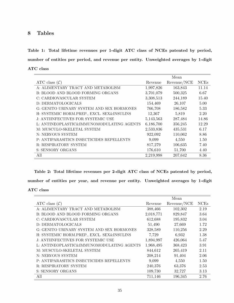
Table 1: Total lifetime revenues per 1-digit ATC class of NCEs patented by period,

number of entities per period, and revenue per entity. Unweighted averages by 1-digit

ATC class

MeanATC class (C) Revenue Revenue/NCE NCEs

A: ALIMENTARY TRACT AND METABOLISM 1,997,826 163,843 11.14B: BLOOD AND BLOOD FORMING ORGANS 3,701,079 500,325 6.67C: CARDIOVASCULAR SYSTEM 3,308,513 244,189 15.40D: DERMATOLOGICALS 154,469 26,107 5.00G: GENITO URINARY SYSTEM AND SEX HORMONES 766,708 186,582 5.33H: SYSTEMIC HORM.PREP., EXCL. SEX&INSULINS 12,367 5,819 2.20J: ANTIINFECTIVES FOR SYSTEMIC USE 5,143,563 287,484 14.86L: ANTINEOPLASTIC&IMMUNOMODULATING AGENTS 6,186,700 356,245 12.29M: MUSCULO-SKELETAL SYSTEM 2,533,836 435,531 6.17N: NERVOUS SYSTEM 922,092 110,062 8.86P: ANTIPARASITICS INSECTICIDES REPELLENTS 9,099 4,550 1.50R: RESPIRATORY SYSTEM 817,279 106,635 7.40S: SENSORY ORGANS 176,610 51,700 4.40

All 2,219,998 207,642 8.36

Table 2: Total lifetime revenues per 2-digit ATC class of NCEs patented by period,

number of entities per year, and revenue per entity. Unweighted averages by 1-digit

ATC class

MeanATC class (C) Revenue Revenue/NCE NCEs

A: ALIMENTARY TRACT AND METABOLISM 388,466 102,302 2.19B: BLOOD AND BLOOD FORMING ORGANS 2,018,771 829,847 3.64C: CARDIOVASCULAR SYSTEM 612,688 195,832 3.04D: DERMATOLOGICALS 51,490 27,669 1.72G: GENITO URINARY SYSTEM AND SEX HORMONES 328,589 110,256 2.29H: SYSTEMIC HORM.PREP., EXCL. SEX&INSULINS 7,729 6,932 1.38J: ANTIINFECTIVES FOR SYSTEMIC USE 1,894,997 426,064 5.47L: ANTINEOPLASTIC&IMMUNOMODULATING AGENTS 1,968,495 368,423 3.91M: MUSCULO-SKELETAL SYSTEM 844,612 265,419 2.11N: NERVOUS SYSTEM 208,214 91,404 2.06P: ANTIPARASITICS INSECTICIDES REPELLENTS 9,099 4,550 1.50R: RESPIRATORY SYSTEM 240,376 63,376 2.53S: SENSORY ORGANS 109,730 32,727 3.13

All 711,146 196,345 2.76

35

Table 3: Definition of Instrument Sets

Set Instruments

A · GDP per capita of corresponding countries· Male and Female Population of corresponding countries· Male and Female Deaths of corresponding ATC-1 class and countries

B · GDP per capita of corresponding countries· Population aged 50 and over of corresponding countries, interacted with ATC-1

C · GDP per capita of corresponding countries· Male Population aged 50 and over of corresponding countries, interacted with ATC-1

D · GDP per capita of corresponding countries· Male Population aged 50 and over of corresponding countries, interacted with ATC-2· Female Population aged 50 and over of corresponding countries, interacted with ATC-2

36

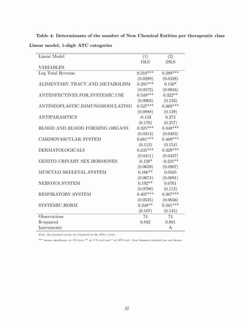
Table 4: Determinants of the number of New Chemical Entities per therapeutic class

Linear model, 1-digit ATC categories

Linear Model (1) (2)OLS 2SLS

VARIABLES

Log Total Revenue 0.216*** 0.289***(0.0289) (0.0428)

ALIMENTARY TRACT AND METABOLISM 0.291*** 0.150*(0.0572) (0.0834)

ANTIINFECTIVES FOR SYSTEMIC USE 0.549*** 0.322**(0.0903) (0.133)

ANTINEOPLASTIC IMMUNOMODULATING 0.527*** 0.369***(0.0888) (0.129)

ANTIPARASITICS -0.133 0.274(0.170) (0.257)

BLOOD AND BLOOD FORMING ORGANS 0.325*** 0.348***(0.0314) (0.0383)

CARDIOVASCULAR SYSTEM 0.681*** 0.469***(0.112) (0.154)

DERMATOLOGICALS 0.245*** 0.329***(0.0411) (0.0427)

GENITO URINARY SEX HORMONES -0.128* -0.221**(0.0659) (0.0907)

MUSCULO SKELETAL SYSTEM 0.166** 0.0585(0.0674) (0.0891)

NERVOUS SYSTEM 0.192** 0.0761(0.0788) (0.112)

RESPIRATORY SYSTEM 0.407*** 0.367***(0.0525) (0.0656)

SYSTEMIC HORM 0.248** 0.561***(0.107) (0.145)

Observations 74 74R-squared 0.832 0.801Instruments A

Note: All standard errors are clustered at the ATC-1 level.

*** means significance at 1% level, ** at 5 % level and * at 10% level. Year dummies included are not shown.

37

Table 5: Determinants of the number of NCEs per therapeutic class Linear model,

2-digit ATC categories

Linear Model (3) (4) (5) (6)OLS 2SLS 2SLS 2SLS

VARIABLES

Log Revenue 0.0962*** 0.0875*** 0.0883*** 0.114***(0.0106) (0.0125) (0.0124) (0.0164)

ALIMENTARY TRACT AND METABOLISM -0.577*** -0.208*** -0.207*** -0.191***(0.124) (0.0201) (0.0201) (0.0214)

ANTIINFECTIVES FOR SYSTEMIC USE -0.162 0.250*** 0.248*** 0.175***(0.147) (0.0426) (0.0420) (0.0470)

ANTINEOPLASTIC IMMUNOMODULATING -0.245 0.148*** 0.147*** 0.103***(0.140) (0.0311) (0.0308) (0.0322)

ANTIPARASITICS -0.685*** -0.349*** -0.347*** -0.276***(0.145) (0.0372) (0.0369) (0.0488)

BLOOD AND BLOOD FORMING ORGANS -0.352** 0.0375 0.0365 0.00354(0.141) (0.0355) (0.0355) (0.0392)

CARDIOVASCULAR SYSTEM -0.347** 0.0304 0.0302 0.0224(0.147) (0.0256) (0.0257) (0.0309)

DERMATOLOGICALS -0.698*** -0.339*** -0.338*** -0.305***(0.119) (0.0360) (0.0359) (0.0387)

GENITO URINARY SEX HORMONES -0.493*** -0.129*** -0.128*** -0.109***(0.132) (0.0305) (0.0305) (0.0325)

MUSCULO SKELETAL SYSTEM -0.567*** -0.196*** -0.196*** -0.171***(0.121) (0.0313) (0.0313) (0.0333)

NERVOUS SYSTEM -0.654*** -0.284*** -0.283*** -0.270***(0.122) (0.0297) (0.0297) (0.0302)

RESPIRATORY SYSTEM -0.356** 0.00421 0.00524 0.0394(0.128) (0.0227) (0.0226) (0.0262)

SYSTEMIC HORM -0.559*** -0.204*** -0.202*** -0.119(0.0809) (0.0772) (0.0772) (0.0891)

Observations 231 231 231 231R-squared 0.715 0.458 0.459 0.465Instruments B C D

Note: All standard errors are clustered at the ATC-1 level.

*** means significance at 1% level, ** at 5 % level and * at 10% level. Year dummies included are not shown.

38

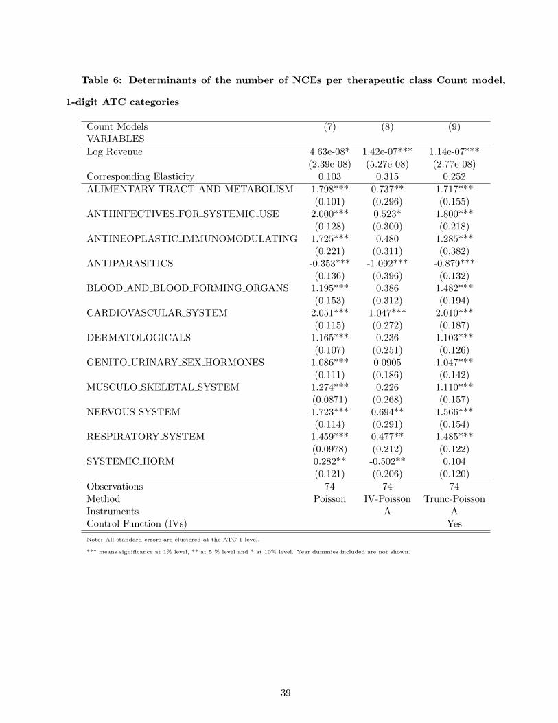
Table 6: Determinants of the number of NCEs per therapeutic class Count model,

1-digit ATC categories

Count Models (7) (8) (9)VARIABLES

Log Revenue 4.63e-08* 1.42e-07*** 1.14e-07***(2.39e-08) (5.27e-08) (2.77e-08)

Corresponding Elasticity 0.103 0.315 0.252

ALIMENTARY TRACT AND METABOLISM 1.798*** 0.737** 1.717***(0.101) (0.296) (0.155)

ANTIINFECTIVES FOR SYSTEMIC USE 2.000*** 0.523* 1.800***(0.128) (0.300) (0.218)

ANTINEOPLASTIC IMMUNOMODULATING 1.725*** 0.480 1.285***(0.221) (0.311) (0.382)

ANTIPARASITICS -0.353*** -1.092*** -0.879***(0.136) (0.396) (0.132)

BLOOD AND BLOOD FORMING ORGANS 1.195*** 0.386 1.482***(0.153) (0.312) (0.194)

CARDIOVASCULAR SYSTEM 2.051*** 1.047*** 2.010***(0.115) (0.272) (0.187)

DERMATOLOGICALS 1.165*** 0.236 1.103***(0.107) (0.251) (0.126)

GENITO URINARY SEX HORMONES 1.086*** 0.0905 1.047***(0.111) (0.186) (0.142)

MUSCULO SKELETAL SYSTEM 1.274*** 0.226 1.110***(0.0871) (0.268) (0.157)

NERVOUS SYSTEM 1.723*** 0.694** 1.566***(0.114) (0.291) (0.154)

RESPIRATORY SYSTEM 1.459*** 0.477** 1.485***(0.0978) (0.212) (0.122)

SYSTEMIC HORM 0.282** -0.502** 0.104(0.121) (0.206) (0.120)

Observations 74 74 74Method Poisson IV-Poisson Trunc-PoissonInstruments A AControl Function (IVs) Yes

Note: All standard errors are clustered at the ATC-1 level.

*** means significance at 1% level, ** at 5 % level and * at 10% level. Year dummies included are not shown.

39

Table 7: Determinants of the number of NCEs per therapeutic class Count model,

2-digit ATC categories

Count Models (10) (11) (12)VARIABLES

Log revenue 8.85e-08*** 4.28e-08 1.47e-07***(1.87e-08) (4.35e-08) (2.20e-08)

Corresponding Elasticity 0.0630 0.0305 0.104

ALIMENTARY TRACT AND METABOLISM 0.382*** 0.0779 0.0211(0.125) (0.111) (0.165)

ANTIINFECTIVES FOR SYSTEMIC USE 1.314*** 1.329*** 1.068***(0.0998) (0.111) (0.119)

ANTINEOPLASTIC IMMUNOMODULATING 0.861*** 1.019*** 0.698***(0.151) (0.0955) (0.135)

ANTIPARASITICS -0.0607 -0.780*** -0.849***(0.184) (0.129) (0.226)

BLOOD AND BLOOD FORMING ORGANS 0.774*** 0.755*** 0.531***(0.156) (0.235) (0.131)

CARDIOVASCULAR SYSTEM 0.683*** 0.484*** 0.401**(0.139) (0.119) (0.183)

DERMATOLOGICALS 0.191 -0.300*** -0.330*(0.121) (0.0962) (0.172)

GENITO URINARY SEX HORMONES 0.411*** 0.133 0.0745(0.138) (0.113) (0.192)

MUSCULO SKELETAL SYSTEM 0.390*** 0.133 -0.0123(0.109) (0.0930) (0.146)

NERVOUS SYSTEM 0.399*** 0.0777 0.0254(0.113) (0.0932) (0.165)

RESPIRATORY SYSTEM 0.510*** 0.260** 0.208(0.140) (0.118) (0.187)

SYSTEMIC HORM 0.188*** -0.562*** -0.603***(0.0730) (0.0864) (0.117)

Observations 231 231 231Method Poisson Trunc-Poisson Trunc-PoissonInstruments A DControl Function (IVs) Yes Yes

Note: All standard errors are clustered at the ATC-1 level.

*** means significance at 1% level, ** at 5 % level and * at 10% level. Year dummies included are not shown.

40

Table 8: Elasticties and Market Size Generating One Innovation per class

Mean Mean

ATC class (C) Elasticity Market SizePer Innovation

A: ALIMENTARY TRACT AND METABOLISM 0.155 1,729,303B: BLOOD AND BLOOD FORMING ORGANS 0.069 15,637,100C: CARDIOVASCULAR SYSTEM 0.098 3,134,607D: DERMATOLOGICALS 0.245 160,228G: GENITO URINARY SYSTEM AND SEX HORMONES 0.269 726,358J: ANTIINFECTIVES FOR SYSTEMIC USE 0.281 3,033,395L: ANTINEOPLASTIC&IMMUNOMODULATING AGENTS 0.377 2,313,080M: MUSCULO-SKELETAL SYSTEM 0.151 3,950,014N: NERVOUS SYSTEM 0.398 386,187R: RESPIRATORY SYSTEM 0.109 1,258,170S: SENSORY ORGANS 0.406 148,508

All 0.231 2,471,139

Table 9: International Classification of Diseases and ATC drug categories

ATC Class ICD10 Disease TitleChapter Blocks

A14, A16 IV E00-E90 Endocrine, nutritional and metabolic diseasesOther A XI K00-K93 Diseases of the digestive systemB III D50-D89 Diseases of the blood and blood-forming organs

and certain disorders involving the immune mechanismC IX I00-I99 Diseases of the circulatory systemD XII L00-L99 Diseases of the skin and subcutaneous tissueG XIV N00-N99 Diseases of the genitourinary systemH IV E00-E90 Endocrine, nutritional and metabolic diseasesJ I A00-B99 Certain infectious and parasitic diseasesL II C00-D48 NeoplasmsM XIII M00-M99 Diseases of musculoskeletal system and connective tissueN1,N2,N3 VI G00-G99 Diseases of the nervous systemN4,N5,N6,N7 V F00-F99 Mental and behavioral disordersP I A00-B99 Certain infectious and parasitic diseasesR X J00-J99 Diseases of the respiratory systemS1 VII H00-H59 Diseases of the eye and adnexaS2 VIII H60-H95 Diseases of the ear and mastoid process

41

9 Appendix 1: Equilibrium Values of N

To find consumer demand in the model of Section 2, note that a consumer located at point c between

firm i and firm i+ 1 and who is indifferent between the two will derive utility Uc where

Uc = vi − pi − t(c− i

N

)= vi+1 − pi+1 − t

(i+ 1

N− c)

from which we can define c, the location of the indifferent consumer under market coverage, as

c =i

N+

1

2N+vi − vi+1 − (pi − pi+1)

2t

In a symmetric equilibrium in which all firms’ prices and qualities are identical, this means that the

utility of the marginal consumer becomes

Uc = vi − pi −t

2N(1)

Now, consider what happens if market coverage does not obtain. Then the indifferent consumer is

defined by

vi − pi − t(c′ − i

N

)= 0

where c′ is the marginal consumer in the absence of market coverage. This implies that

c′ =i

N+

(vi − pi)t

Now consider the objective function Πi of firm i. When the quality of products is exogenous and

market coverage is complete, profits of firm i are:

Πi = mpi

(1

N+

2vi − vi−1 − vi+1 −(2pi − pi−1−pi+1

)2t

)−K

Taking first order conditions with respect to prices while qualities are fixed yields:

∂Πi

∂pi= m

(1

N+

2vi − (vi−1 + vi+1) +(pi−1+pi+1

)2t

− 2pit

)= 0

pi =2t

N+(pi−1+pi+1

)+ 2vi − (vi−1 + vi+1)

In a symmetric equilibrium where qualities and prices are identical among firms, this implies that

pi =t

2N(2)

42

We can now use the zero-profit condition to solve for the equilibrium value of N (ignoring integer

problems). Substituting for equilibrium prices in the profit function yields

Πi =mt

2N2−K

which when profits are zero implies

N =

√mt

2K(3)

Then, industry profits are zero and industry revenue is NK.

This yields a monotonic, strictly concave, relationship between potential demandm and the number

of firms N (hence of pharmaceutical products in the market), with N proportional to the square root

of m. From this we can derive

∂N

∂m=

1

2

√t

2mK=

N

2m(4)

which implies that the elasticity of N with respect to m is 0.5.

To verify the conditions under which this is consistent with market coverage, note that substituting

(2) into (1) implies that the indifferent consumer c has utility level

Uc = vi −t

N

which for market coverage with exogenous quality implies, by substitution of (3), that

vi ≥

√2tK

m

So we can conclude that, if quality is exogenous and above some threshold (√

2tKm ) that is increasing

in the extent of product differentiation (t) and in fixed entry costs (K), and decreasing in potential

demand (m), then the number of drugs in the market increases as the square root of potential demand.

To conclude the analysis of the case with exogenous quality, we note that if the market were not

fully covered, prices would be given by the expression

pi =vi2

43

Then, the profit function becomes

Πi =mvi

2

4= K

which implies that fixed costs of entry are either too high so that no entry occurs, or low enough so that

entry occurs until it exhausts all available opportunities. For constant fixed cost, this suggests that

market coverage is the only interesting case to study. For fixed costs that vary by potential demand,

entry will be determined entirely by the shape of the cost function: any increase in m will simply raise

the profit threshold for entry, and all firms with fixed costs below the new higher threshold will enter.

In studying endogenous quality, we therefore look only at the case of full market coverage. Then,

the profit function can be written as follows:

Πi = mpi

(1

N+

2vi − vi−1 − vi+1 −(2pi − pi−1−pi+1

)2t

)−(K +

γ(vi − v)2

2

)

where K + γ(vi−v)2

2 is the cost of innovating with an innovation of quality level vi.

This differs from the profit function when quality is exogenous only in that the fixed cost contains

an element that is quadratic in the cost of increasing quality above a certain base level v.

Assume that firms first choose product quality as part of their R&D decisions, then choose prices

once qualities are fixed. When choosing their R&D decisions they take the R&D decisions of other

firms as fixed and therefore also their entry decisions, so N is taken as given by firms choosing quality.

In solving for prices we can no longer presume equilibrium is symmetric. We assume nevertheless

that equilibrium is symmetric among firms other than firm i. Writing pj = pi+1 = pi−1 and analogously

for qualities, taking first order conditions with respect to pi and substituting in the analogous first

order conditions for pj yields

pi =t

N+

2 (vi − vj)3

Substituting for prices in the objective function yields

Πi = m

(t

N+

(vi − vj)3

)(1

N+vi − vj

3t

)−(K +

γ(vi − v)2

2

)

and taking first order conditions with respect to vi yields

m

N+

4m (vi − vj)9t

+ γv − γvi = 0

44

which, since equilibrium is symmetric, implies that

vi = v +m

γN

This incidentally implies that the condition for market coverage can be written as

v +m

γN− t

N− t

2N≥ 0

which implies a threshold condition for v, namely that v ≥ 3tγ−2m2γN .

We can now use the zero-profit condition to solve for the equilibrium value of N , denoted N∗.

Substituting for equilibrium qualities and prices in the profit function yields

Πi =mt

N2−(K +

m2

2γN2

)

which when profits are zero implies

N∗ =

√mt

K

(1− m

2tγ

)

A real solution for N∗ requires that γ ≥ m2t , which will hold so long as the cost of improving the

product is sufficiently great.

Then, we also have the equilibrium quality of products which is

vi = v +1

γ

√mK

t− m2γ

which is increasing in K, decreasing in γ, t.

We can then differentiate N∗ with respect to m to yield:

∂N

∂m=

t− mγ

2

√mtK

(1− m

2tγ

)which is strictly positive so long as γ > m/2t.

With endogenous quality, we no longer find a unit elasticity of the number of firms (or drugs) N∗

with respect to total revenue. In this case, total market revenue R∗ is endogenous and given as a

function of endogenous N∗ by

R∗ (N∗,m) =

(K +

m2

2γN∗2

)N∗ = KN∗ +

m2

2γN∗

45

which is a U shaped function of N∗ with a minimum at m√2γK

. It is useful to note that as γ → ∞ it

converges to the expression for revenue under exogenous fixed costs.

However, since for a real solution for N it is necessary that γ ≥ m2t , R

∗ (N∗,m) is increasing in N

at the optimal N∗ because

∂

∂NR∗ (N∗,m) = K − m2

2γN∗2= K

(1− 1

2γ tm − 1

)> 0

This means that the relationship between N∗ and R∗ is increasing for a given m.

Now, as R∗ (N∗ (m) ,m) is increasing because

dR∗ (N∗ (m) ,m)

dm=∂R∗ (N∗,m)

∂N

∂N∗

∂m+∂R∗ (N∗,m)

∂m> 0

since

∂N∗

∂m=

t− mγ

2

√mtK

(1− m

2tγ

) > 0

and

∂R∗ (N∗,m)

∂m=

m

γN∗> 0

we can define m(R∗) as the inverse of R∗ (N∗ (m) ,m). The function m(R∗) is increasing in R∗ and

we thus have that∂N∗

∂R∗ = ∂N∗

∂m∂m∂R∗ > 0.

It follows therefore that the number of equilibrium firms will also be an increasing function of total

market revenue.

46

10 Appendix 2:

Table A1: First stage Regressions

Part I First Stage OLS

(1) (2) (3) (4) (5)N tc N t

c N tc′ N t

c′ N tc′

Exogenous VariablesATC 1 DummiesATC=A -671,704 717,025 -148,967 -153,311 100,283

(451,203) (416,881) (95,638) (93,969) (72,699)

ATC=J 1.254e+06 205,389 849,167*** 723,041*** -454,158***

(821,051) (537,990) (68,507) (71,614) (63,226)

ATC=L -546,485 -3.801e+06 -575,018*** -573,789*** 135,752***

(771,007) (2.211e+06) (50,796) (49,073) (42,162)

ATC=P -2.239e+06*

(1.187e+06)

ATC=B 2.083e+06** 2.003e+06*** 1.686e+06*** 1.444e+06*** 1.392e+06***

(754,732) (362,185) (100,290) (106,505) (74,399)

ATC=C 5.003e+06*** 506,955 -300,247* -289,961 -439,992***

(937,328) (338,806) (163,582) (175,303) (96,491)

ATC=D -1.520e+06* -367,490 60,830 51,564 -130,306*

(757,720) (564,292) (62,172) (59,405) (72,048)

ATC=G 138,386 175,317 654,693*** 640,614*** 334,121

(504,961) (645,072) (108,245) (108,539) (197,568)

ATC=M 981,497 -116,282 220,161* 182,896 -183,162**

(763,029) (330,478) (114,200) (118,717) (60,174)

ATC=N -395,630 1.269e+06 181,970** 177,085** -76,545

(714,891) (1.762e+06) (69,962) (68,877) (95,652)

ATC=R -2.723e+06*** -459,268 -201,126 -212,768 -154,221

(555,035) (830,902) (166,551) (168,083) (95,846)

ATC=H -716,467 3.279e+06 -72,251 -83,674 -71,128

(538,355) (5.187e+06) (97,227) (110,306) (59,435)

Note: All standard errors (shown in brackets) are clustered at the ATC-1 level. Time dummies included

***, **, * means significance at 1%, 5 % and 10% levels

47

Table A1 - Continued 1

Part II First Stage OLS

(1) (2) (3) (4) (5)N tc N t

c N tc′ N t

c′ N tc′

Excluded IVsMale population 0.109**

Female population -0.108*

Nb of Deaths -4.135***

Nb of Male Deaths 8.380***

GDP 6.31e-08

Observations 74 74 231 231 231

R-squared 0.800 0.971 0.435 0.421 0.550

IVs A D B C D

Test Excluded. IVs

F test 60.80 46.61 886.4 1044 40.25

P value 4.19e-08 1.90e-07 0 0 4.32e-07

Excluded IVsMale Pop Above 50 in countries

served by drugs of own ATC-2 level times ATC-1 dummy

Male Pop Above 50*ATC=A -0.274** 0.0389***

Male Pop Above 50*ATC=J -0.193 0.0497***

Male Pop Above 50*ATC=L 0.121 0.108***

Male Pop Above 50*ATC=B 0.930*** 0.0619*

Male Pop Above 50*ATC=C 1.297*** 0.0697***

Male Pop Above 50*ATC=D 0.0914 0.0326

Male Pop Above 50*ATC=G 0.317 0.0694***

Male Pop Above 50*ATC=M 0.142 0.220***

Male Pop Above 50*ATC=N -0.0133 0.0272**

Male Pop Above 50*ATC=R -0.0844 0.0666***

Male Pop Above 50*ATC=S -0.105 -0.0316

Male Pop Above 50*ATC=H -0.453 0.0265

Excluded IVsFemale Pop Above 50 in countries

served by drugs of own ATC-2 level times ATC-1 dummy

Female Pop Above 50*ATC=A 0.184** -0.0366***

Female Pop Above 50*ATC=J 0.246 -0.0198*

Female Pop Above 50*ATC=L -0.241 -0.0889***

Female Pop Above 50*ATC=P 0.000752 -0.00666

Female Pop Above 50*ATC=B -0.965*** -0.0883**

Female Pop Above 50*ATC=C -1.137*** -0.0551***

Female Pop Above 50*ATC=D -0.0902 -0.0305

Female Pop Above 50*ATC=G -0.269 -0.0593***

Female Pop Above 50*ATC=M -0.146* -0.192***

Female Pop Above 50*ATC=N 0.0261 -0.0262**

Female Pop Above 50*ATC=R 0.0928 -0.0564***

Female Pop Above 50*ATC=S 0.0882 0.0352

Female Pop Above 50*ATC=H 0.440 -0.0208

Note: All standard errors (not shown) are clustered at the ATC-1 level.

***, **, * means significance at 1%, 5 % and 10% levels

48

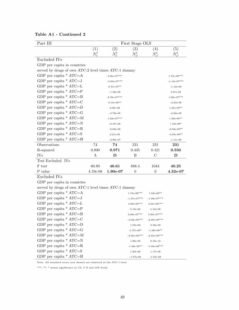
Table A1 - Continued 2

Part III First Stage OLS

(1) (2) (3) (4) (5)N tc N t

c N tc′ N t

c′ N tc′

Excluded IVsGDP per capita in countries

served by drugs of own ATC-2 level times ATC-1 dummy

GDP per capita * ATC=A 3.06e-07*** 1.72e-08***

GDP per capita * ATC=J -4.00e-07*** -1.12e-07***

GDP per capita * ATC=L 8.31e-07** -1.12e-08

GDP per capita * ATC=P -1.22e-08 2.91e-08

GDP per capita * ATC=B 8.78e-07*** 1.98e-07***

GDP per capita * ATC=C 9.15e-08** -2.24e-08

GDP per capita * ATC=D 6.09e-08 1.25e-08**

GDP per capita * ATC=G -3.78e-08 -4.82e-09

GDP per capita * ATC=M 1.62e-07*** 1.29e-08**

GDP per capita * ATC=N -8.47e-08 1.59e-08*

GDP per capita * ATC=R -9.08e-08 -6.93e-09**

GDP per capita * ATC=S 2.21e-08 -4.05e-08**

GDP per capita * ATC=H -2.90e-07 -1.11e-08

Observations 74 74 231 231 231

R-squared 0.800 0.971 0.435 0.421 0.550

IVs A D B C D

Test Excluded. IVs

F test 60.80 46.61 886.4 1044 40.25

P value 4.19e-08 1.90e-07 0 0 4.32e-07

Excluded IVsGDP per capita in countries

served by drugs of own ATC-1 level times ATC-1 dummy

GDP per capita * ATC=A 1.74e-08*** 1.62e-08**

GDP per capita * ATC=J -1.27e-07*** -1.09e-07***

GDP per capita * ATC=L 4.08e-08*** 3.84e-08***

GDP per capita * ATC=P 5.18e-08 5.10e-08

GDP per capita * ATC=B 6.68e-07*** 5.80e-07***

GDP per capita * ATC=C -3.02e-08*** -2.96e-08***

GDP per capita * ATC=D 1.03e-08 9.22e-09

GDP per capita * ATC=G -1.27e-08* -1.28e-08**

GDP per capita * ATC=M -2.50e-08*** -2.65e-08***

GDP per capita * ATC=N 1.86e-09 8.16e-10

GDP per capita * ATC=R -1.28e-08** -1.58e-08***

GDP per capita * ATC=S 1.29e-08 1.17e-08

GDP per capita * ATC=H -1.67e-08 -1.95e-08

Note: All standard errors (not shown) are clustered at the ATC-1 level.

***, **, * means significance at 1%, 5 % and 10% levels

49

Table A1 - Continued 3

Part IV First Stage OLS

(1) (2) (3) (4) (5)N tc N t

c N tc′ N t

c′ N tc′

Excluded IVsPop Above 50 in countries

served by drugs of own ATC-1 level times ATC-1 dummy

Pop Above 50 * ATC=A -0.00131**

Pop Above 50 * ATC=J 0.0123***

Pop Above 50 * ATC=L -0.00234***

Pop Above 50 * ATC=P -0.00572

Pop Above 50 * ATC=B -0.0648***

Pop Above 50 * ATC=C 0.00334***

Pop Above 50 * ATC=D -0.00100

Pop Above 50 * ATC=G 0.000935

Pop Above 50 * ATC=M 0.00277***

Pop Above 50 * ATC=N -0.000140

Pop Above 50 * ATC=R 0.00159***

Pop Above 50 * ATC=S -0.00110

Pop Above 50 * ATC=H 0.00183

Excluded IVsMale pop Above 50 in countries

served by drugs of own ATC-1 level times ATC-1 dummy

Male Pop Above 50*ATC=A -0.00259**

Male Pop Above 50*ATC=J 0.0229***

Male Pop Above 50*ATC=L -0.00457***

Male Pop Above 50*ATC=P -0.0123

Male Pop Above 50*ATC=B -0.121***

Male Pop Above 50*ATC=C 0.00702***

Male Pop Above 50*ATC=D -0.00196

Male Pop Above 50*ATC=G 0.00203

Male Pop Above 50*ATC=M 0.00627***

Male Pop Above 50*ATC=N -0.000102

Male Pop Above 50*ATC=R 0.00399***

Male Pop Above 50*ATC=S -0.00215

Male Pop Above 50*ATC=H 0.00452

Observations 74 74 231 231 231

R-squared 0.800 0.971 0.435 0.421 0.550

IVs A D B C D

Test Excluded. IVs

F test 60.80 46.61 886.4 1044 40.25

P value 4.19e-08 1.90e-07 0 0 4.32e-07

Note: All standard errors (not shown) are clustered at the ATC-1 level.

***, **, * means significance at 1%, 5 % and 10% levels

50

Figure 1: Total Revenue and New Chemical Entities per 1-digit ATC class

51

0.5

11

.5

4 5 6 7 8 9 10 11 12 13 14 15 16 17 18 19 20

A0

.51

1.5

1 2 3 4 5 6 7 8 9 10 11 12 13 14 15 16 17 18 19 20

B

0.5

11

.52

1 2 3 4 5 6 7 8 9 10 11 12 13 14 15 16 17 18 19 20

C

0.5

11

.52

2.5

3 4 5 6 7 8 9 10 11 12 13 14 15 16 17 18 19 20

D

0.5

11

.5

2 3 4 5 6 7 8 9 10 11 12 13 14 15 16 17 18 19 20

G

02

46

6 7 8 9 10 11 12 13 14 15 16 17 18 19 20

H

0.2

.4.6

.81

1 2 3 4 5 6 7 8 9 10 11 12 13 14 15 16 17 18 19 20

J

0.5

11

.5

1 2 3 4 5 6 7 8 9 10 11 12 13 14 15 16 17 18 19 20

L

0.2

.4.6

.81

1 2 3 4 5 6 7 8 9 10 11 12 13 14 15 16 17 18 19 20

M

01

23

3 4 5 6 7 8 9 10 11 12 13 14 15 16 17 18 19 20

N

02

46

8

8 9 10 11 12 13 14 15 16 17 18 19 20

P

01

23

1 2 3 4 5 6 7 8 9 10 11 12 13 14 15 16 17 18 19 20

R

0.5

11

.52

5 6 7 8 9 10 11 12 13 14 15 16 17 18 19 20

S

Figure 2: Means of Revenue by Patent Age for Each ATC-1

52