Embed Size (px)
Citation preview
Market Size and Pharmaceutical Innovation
Pierre Dubois∗, Olivier de Mouzon†, Fiona Scott-Morton‡, Paul Seabright§
This Version: October 2011¶
Abstract
This paper quantifies the relationship between market size and innovation in the pharmaceuticalindustry using improved, and newer, methods and data. We estimate the elasticity of innovation,as measured by the number of new chemical entities appearing on the market for a given diseaseclass, to the expected market size as measured by the spending of sufferers of diseases in that class(and others acting on their behalf such as insurers and governments) on their treatment during thepatent lifetime. We find positive significant elasticities with a point estimate under our preferredspecification of 25.2%. This suggests that, on average, at the mean market size an additional$1.8 billion is required in additional patent life revenue to support the invention of one additionalnew chemical entity. An elasticity substantially and significantly below 100% is also a plausibleimplication of the hypothesis that innovation in pharmaceuticals is becoming more diffi cult andexpensive over time, as costs of regulatory approval rise and as the industry runs out of "lowhanging fruit".
Key words: Innovation, Market Size, Elasticity, Pharmaceuticals.
JEL codes: O31, L65, O34.
∗Toulouse School of Economics (GREMAQ, IDEI), [email protected]†Toulouse School of Economics (GREMAQ, INRA), [email protected]‡Yale University, [email protected]§Toulouse School of Economics (GREMAQ, IDEI), [email protected]¶We thank Tamer Abdelgawad, Amber Batata, Bruno Jullien, Bernard Salanié and seminar participants at Toulouse,
PEPC Paris, Imperial College London for useful comments. We thank SCIFI-GLOW: SCience, Innovation, FIrms andmarkets in a GLObalized World, Contract no. SSH7-CT-2008-217436. The statements, findings, conclusions, views, andopinions contained and expressed in this article are based in part on data obtained under license from the following IMSHealth Incorporated information service(s): MIDASTM (1997—2007), IMS Health Incorporated. All Rights Reserved.The statements, findings, conclusions, views, and opinions contained and expressed herein are not necessarily those ofIMS Health Incorporated or any of its affi liated or subsidiary entities. We also thank Pfizer Inc for its center researchsupport to IDEI. The statements, findings, conclusions, views and opinions contained and expressed herein are those ofthe authors only.
1

1 Introduction
This paper quantifies the relationship between financial returns and innovation in the pharmaceutical
industry. More precisely we shall estimate the elasticity of innovation (as measured by the number of
new chemical entities appearing on the market for a given disease class) to the expected market size as
measured by the spending on treatment by sufferers of diseases in that class (and others acting on their
behalf such as insurers and governments). While this is an important question that has been addressed
in earlier literature, we believe our paper improves on that literature in several important ways. First,
we have data on the names and the global revenues of all pharmaceutical products over an eleven year
period, as collected by a pharmaceutical data provider IMS. These detailed data allow us to calculate
an excellent measure of innovation, the number of new molecular entities released during our time
period. Literature prior to the availability of this dataset proxies for innovation with intermediate
measures such as clinical trials or available regimens, or counts only drug products released in the
United States. Global revenue data have never, to our knowledge, been used in the literature to
measure the response of innovation to market size but yet are likely one of the most useful available
measures of market size. Secondly, we employ new methods to estimate the relationship between
innovation and market size. Our empirical technique is designed to obtain unbiased estimates from
censored count data. In addition, it accommodates our instrumental variables strategy, also new in
the literature. While a large expected market size may stimulate new pharmaceutical innovation,
it may also be the case that new pharmaceutical innovation creates sales and therefore market size.
New innovation also intensifies competition between products and therefore reduces prices and the
overall proportion of consumer willingness to pay that producers can expect to appropriate. Because
of the likely existence of reverse causality, we instrument for market size in our estimation procedure.
We find, not surprisingly, that market size has a positive impact on global release of new molecular
entities. However, our elasticity estimate is very substantially below unity, which implies (as we explain
in the theoretical section) that if our model of innovation is accurate the fixed costs of innovation are
rising sharply with market size. We follow up this estimate with regressions specific to a therapeutic
class. Although there is significant variation between therapeutic classes, and the average elasticity
2
across classes is somewhat higher than that estimated by pooling classes, this elasticity still implies
significantly rising innovation costs with market size.
Expected market size is influenced by broadly three types of factors. First there are factors such as
demographic and socio-economic change, which affect the numbers of people who are likely to suffer
from a particular medical condition and the resources they are likely to have available to spend on
alleviating their condition. A motivating example concerning research on gout from the New York
Times illustrates the incentives for R&D. "Often called the “disease of kings”because of its association
with the rich foods and copious alcohol once available only to aristocrats, gout is staging a middle-class
comeback as American society grows older and heavier. ...Companies are now racing to improve upon
decades-old generic drugs that do not work well for everyone. Already this year the Food and Drug
Administration has approved the first new gout drug in more than 40 years...".1 Many other examples
evidently spring to mind of research motivated primarily by changing demographic and socio-economic
factors, such as research into cardiovascular disease and Alzheimer’s disease. We shall refer to such
factors in the paper as "potential demand".
Secondly, there are factors particular to the pharmaceutical and health-care industries, such as
the degree of competition among firms and the strategies that firms use to innovate, cut costs, and
win customers, that affect the profitability of innovation. For example, intensified competition from
generics for branded products occurs not only as a response to patent expiry but also in response to
the purchasing environments. Cost-control pressures from managed care create incentives for generic
use and reduce the expected market size of an innovation. The response of firms to a given potential
demand may also depend on such considerations as their degree of symmetry in competence: the
competition between two firms of similar size and employing similar talent pools may be quite different
1 "Disease of Rich Extends Its Pain to Middle class", New York Times, June 12, 2009 . The story continued:"...a product called Uloric from Takeda Pharmaceutical. Another new drug, Krystexxa, made by Savient Pharmaceu-
ticals of East Brunswick, N.J., will be reviewed for possible approval by an F.D.A. advisory committee on Tuesday. Andseveral other companies are testing drugs in clinical trials. “It’s kind of like the forgotten disease,”said Barry D. Quart,chief executive of one of those companies, Ardea Biosciences of San Diego. Ardea discovered accidentally that an AIDSdrug it was developing might work against gout. Now the company has shifted its focus to gout, envisioning annual salesof $1 billion if its drug is successful. That would mean a huge increase in spending on gout medicines, which had sales ofonly $53.4 million last year, according to IMS Health, a health care information company. Uloric, the drug from Takeda,sells a daily pill for at least $4.50 compared with 10 to 50 cents for the most commonly used generic, allopurinol. It isestimated that two million to six million Americans have gout... Various studies suggest that the number of cases in thiscountry has as much as doubled in the last three decades".
3
from competition between a leader and a follower firm.
Thirdly, there are public policies, including policies towards intellectual property protection, drug
safety and testing, pricing and reimbursement, and public funding of research. As a matter of compar-
ison, in 2004, research spending by NIH reached $28.5 billion while the members of the Pharmaceutical
Research and Manufacturers of America report R&D spending of about $40 billion - see CBO 2006.
Policy innovations such as the introduction of Medicare in the 1960s have had a large impact on ex-
pected market size, and various researchers have noted the consequences for research and innovation
in drugs for the elderly that were the probable consequence (Acemoglu et al., 2006).
In principle it might be thought that, from a policy point of view, the only really interesting factors
affecting expected market size are those in the third category, and that therefore any study such as
ours should focus on the elasticity of innovation with respect to these factors only. Such estimates
could be used, for instance, to calculate the social cost of a particular drug pricing regime or of a
proposed change in the length or breadth of patent protection, or the social returns to additional
spending by the NIH. However, this argument is flawed, even if one ignores the possibility that the
influence of the other types of factor may be of independent interest (such as for predicting future
trends in research and innovation). Estimating the elasticity of innovation with respect to past changes
in policy would be possible only if we could observe genuine policy experiments, conducted without
reference to the many factors, unobserved to the econometrician, that might influence the potential
rate of innovation. But most policy changes are not like that, and arguably most of them should not
be. They are typically endogenous to the rate of innovation itself, either because public policy may
feel it does not need to intervene to favor areas where innovation is already coming along nicely, or
because public policy likes to bask in the glow of supporting visibly successful areas, or because once
key drugs have been developed it is tempting to lower their prices to users, or for any number of
other reasons. This makes the observed elasticity of innovation with respect to past policy changes
unreliable as a guide to the elasticity of innovation with respect to future policy changes.
Factors of the first type, by contrast, are rarely under the influence of either government or industry
participants, at least not in the short- to medium-term. We exploit these exogenous changes in
4

potential demand to estimate elasticities, freed from the confusing interference on expected market
size of the two other types of factor. We examine the response of global new drug launches to global
expected market size measured in revenues. Of course, a simple regression of new drugs on revenues will
pick up both causal directions mentioned above: revenues attract innovation and also drug innovations
generate revenue. Our identification strategy is as follows. If the cardiovascular market is expected to
grow due to an aging population, firms will want to serve that demand. Therefore, there will be an
increase in cardiovascular R&D and - on average - we will see the release of new cardiovascular products
on the market at the time of the demand increase. Different therapeutic markets whose potential sizes
change differently over time due to demographic and income differences drive commensurate changes
in innovative activity. We can measure the elasticity of new products to expected market size using
this variation.
Thus our instruments are measures of population and disease prevalence in our sample of countries
over time. Our strategy is sensible because demographics are strongly correlated with revenue. More-
over, the invention of a new drug does not change the contemporaneous propensity for populations of a
particular country to suffer from cardiovascular disease, for example. One might think that discovery
of an effective innovative product would increase life expectancy and therefore alter the demographic
trends we measure2. However, the fact that we use contemporaneous demographics over a 4 year pe-
riod of time contemporaneous to product launch makes this unlikely and protects us from this reverse
causality. It is not likely that a new product could affect mortality this quickly. Thus we expect
demographics to be uncorrelated with the error term in our regression of new drug counts. For our
assumption to be violated, it must be the case that a novel therapy generates additional measurable
diagnoses in the specific area. While this makes sense for narrowly targeted treatments and diagnoses,
it seems much less likely to be operating at the level of fairly coarse disease areas tracked by WHO,
such as “cardiovascular disease”. By utilizing this instrumental variables approach, we can isolate the
impact of revenue changes driven by demographics and determine their impact on innovation.
We use international data to reflect the fact that all markets, including those outside the US,
constitute an important incentive for innovation. There is an older literature relating market size in2Lichtenberg and Duflos (2008) provides evidence of this channel.
5
a country to the R&D undertaken in that country. Because there are unobserved factors such as the
level of education in a country that might affect both R&D and health spending, we do not use this
source of variation. The variation we exploit is across therapeutic classes and over time, rather than
across geography. Additionally, biopharmaceutical research is carried out all across the globe by both
local and international firms. In our view, therefore, the appropriate level of analysis for a study of
the determinants of innovation —both in terms of which products to include and which markets to
count - is global.
The relatively recent literature on the topic of the elasticity of pharmaceutical innovation to ex-
pected market size contains two broad approaches. The older of the two uses accounting data to
estimate the determinants of R&D (see Grabowski and Vernon (2000)). In theory, under perfect cap-
ital markets R&D would be chosen only in response to expected future profitability of the project.
However, if capital markets are imperfect and external funds are more expensive than internal cash
flow, current revenue (market size) will have a positive impact on the amount of research funded by the
firm. Of course, if current market size is a proxy for future market size, then current research may be
responding to future sales opportunities also, but these two effects cannot be disentangled. Giacotto
et al. (2005) regress R&D-to-sales ratio on the pharmaceutical price index from the previous year and
other variables. Again, this is a model of innovation responding not to expected future market size,
but to recent prices. They find a 1% increase in price leads to a 0.58% increase in R&D spending.
Finkelstein (2004) finds that a 1% increase in revenue for vaccines leads to a (much lower) 0.05% to
0.06% increase in R&D spending on vaccines. A second stream of the literature uses alternate mea-
sures both for outcomes and market size. Innovation is measured as clinical trials (Blume-Kohout and
Sood, 2009; Yin, 2008, 2009), journal articles or disease regimens (Lichtenberg, 2006), while poten-
tial market size is (negative) disability-adjusted life years (DALY) or mortality (Civan and Maloney,
2006,2009, Lichtenberg, 2005). Lichtenberg (2005) finds results of similar magnitude: a 1% increase
in the number of people with cancer leads to a .58% increase in chemotherapy regimens. Civan and
Maloney (2006, 2009) find that a 1% increase in expected US entry price leads to .5% increase in
the number of drugs in the drug development pipeline. Lichtenberg (2005) finds that a 1% increase
6
in DALY leads to a 1.3% increase in global drug launches. Acemoglu and Linn (2004) use variation
from 1970-2000 in the expenditure share of different US age cohorts for different therapeutic classes.
They combine this with data on all US FDA-approved new products and find that a 1% increase in
contemporaneous expenditure shares leads to a 4% increase in the number of new drugs released on
the market. This is a markedly higher elasticity than found in the previous literature.
While we will estimate the impact of financial incentives on the launch of new products, we are
cautious about drawing conclusions about the welfare benefits of those new products. There are
various reasons why this is not straightforward. One is that there may be diminishing marginal health
benefits from innovation: the first radical innovation in a therapeutic class may produce much greater
overall benefits than a drug that is just suffi ciently different from it to be granted a patent (though the
opposite could be true if the second drug avoids debilitating side-effects associated with the first). A
second reason is that it is particularly diffi cult in this line of research to calculate the welfare of a new
innovation in the absence of measures of consumers’valuation or willingness to pay. Most patients
are insured and therefore do not face a marginal price when buying biopharmaceuticals. The buyer
in most cases is either the nation in the case of national health systems, or the large PBMs, in the
case of private healthcare (USA), or some national systems like Germany. This buyer, while not the
patient, is the one that controls the formulary and pays at the margin, and so, from the point of view
of the researcher, has revealed a valuation for the treatment. However, some of these buyers may have
monopsony power and face political constraints, so using negotiated prices may not closely reflect
consumer welfare. An alternative approach to calculating welfare is to simply measure life years saved
by the new innovations and multiply by QALY, though comparable data for many of these products
is sparse. Our elasticities should therefore be interpreted only in terms of new product numbers and
great care should be exercised before any welfare conclusions are explicitly or implicitly drawn from
them.
We begin in section 2 by describing a simple model with testable implications we are investigating.
Section 3 describes our data. Section 4 gives our detailed results. Section 5 concludes.
7
2 Theoretical Framework and Testable Implications
We are interested in the effect of expected market size on innovation. The model will consider that a
market represents a set of products in a given therapeutic class (though in the empirics we shall test
the robustness of our estimates to variations in the breadth of definition of such classes).
Consider the question of how firms expect the share of the potential revenues in a given market to
vary according to their R&D investments. This problem has two parts: how much their investments
will affect either the probability of discovering new drugs or the date at which they are discovered (or
both), and how the discovery of new drugs will affect their revenues given the expected presence of
other drugs on the market. Several simple models can be considered to study this relationship, and
predictions differ according to the assumed exogeneity of the structure of the industry, to the number
of firms, to the cost structure of R&D, and to the existence of R&D spillovers.
One approach which has been used in the previous literature is that drugs within a given therapeutic
category are only vertically differentiated; at any one moment the best drug, and only the best, will
capture the entire market. However, the top drug may not remain the best for long, and ongoing
research may at any moment produce a better drug which will in turn capture the entire market,
reducing the revenues of the previous best drug immediately to zero. The effort of pharmaceutical
research will therefore consist in trying to produce the drugs that are better than existing drugs and
hold that position for long enough to sustain their development costs before the next improved drug
in the class arrives.
We want to include horizontal differentiation in our model for several reasons. First, as a practical
matter, it is clear that many different treatments within the same therapeutic class have positive
revenue in the same time period. This, along with the findings in the clinical literature, indicates
that there is substantial horizontal differentiation in pharmaceutical markets. We want our model
to reflect this feature of the industry. Secondly, we are interested in developing a model that will
demonstrate a link between market size and the number of products. A model that allows the firm
to choose its level of R&D will yield results that depend on the trade-off between horizontal and
vertical product differentiation, issues that are not well explored in a model in which the highest
8

quality product captures the entire market. For instance, Sutton (1991) shows that increasing market
size may not alter concentration in the industry if increased quality successfully attracts consumers
away from horizontally differentiated alternative products. In these circumstances a larger market
size will lead the firm to invest in vertical differentiation which naturally results in higher quality
products, but not in the entry of new firms. The reason is that margins must support the fixed costs
desired by consumers; if they want high quality, then both market share and margins must contribute
to covering those fixed costs, which means concentration must also be high. Increasing the degree of
horizontal differentiation weakens the Sutton result because of the built-in incentive for a firm to serve a
differentiated niche even with lower quality. Berry and Waldfogel (2010) illustrate this trade-off in their
work comparing restaurants to newspapers. Because restaurants are more horizontally differentiated
than newspapers and costs are mostly variable (unlike in newspapers), increasing market size does call
forth new firms and reduce concentration. By contrast, newspaper quality is improved using fixed costs
and newspapers compete on vertical quality measures, so increased market size does not create new
firms but rather raises the quality of incumbents. In their paper, the type of differentiation and the
cost structure have the same response to increased market size and work together to create maximal
difference in outcomes between the two industries. Our setting, pharmaceuticals, has significant
horizontal differentiation but also significant fixed costs, thus not fitting neatly into the Berry and
Waldfogel (2010) framework. We present below a model that allows for both horizontal and vertical
product differentiation, where firms can invest in quality by increasing fixed cost. We show that the
number of firms increases in market size when fixed costs are exogenous. To address the Sutton point,
we repeat the analysis for endogenous fixed costs and find the conditions under which we achieve the
same result.
Lastly, our final point is that therapeutic classes with horizontal differentiation are much easier to
operationalize empirically, a point we will return to below.
2.1 A Simple Model of R&D with Horizontal Differentiation
The model is a version of the well-known circle model due to Salop (1979), extended to incorporate
vertical differentiation in the manner of Armstrong and Weeds (2005). The Salop circle model is a
9

nice choice for our problem because a natural number of firms fit round the circle in response to
consumers’willingness to pay and fixed costs. In this framework, when a firm considers whether it
should invest or not, it forms its expectations about revenues of the product over its lifetime, taking
into account the productivity of its own research programs and those of its rivals. We assume that
firms have rational expectations of the number of rivals, shares and prices.
Consider a circle of unit size, with a mass m of consumers uniformly distributed around the circle.
We shall call this parameter m the "potential demand", and note that it is not the same as actual
market size (or revenue) since the latter will depend on other conditions including prices.
Around this circle N firms are located at equal intervals. Firm i is located at point i/N , and
incurs a fixed cost of investment to produce a drug of quality vi which it sells at price pi; the number
of firms N will be determined by the requirement that the marginal firm makes zero profits (we shall
ignore integer problems).
A consumer purchases at most one unit of the drug, and has an outside option yielding utility
normalized to zero, so will purchase uniquely if doing so yields weakly positive utility. To simplify the
algebra we assume marginal costs of production are zero, though nothing in the qualitative results
turns on this assumption.
Consider what happens if there is market coverage —every consumer buys from at least one firm.
A consumer located at point c between firm i and firm i + 1 and who is indifferent between the two
will derive utility Uc where
Uc = vi − pi − t(c− i
N
)= vi+1 − pi+1 − t
(i+ 1
N− c)
from which we can define c, the location of the indifferent consumer under market coverage, as
c =i
N+
1
2N+vi − vi+1 − (pi − pi+1)
2t
where t is the (linear) “transport cost”, an indicator of the extent of horizontal product differentiation.
In a symmetric equilibrium in which all firms’prices and qualities are identical, this means that the
utility of the marginal consumer becomes
Uc = vi − pi −t
2N(1)
10

Now, consider what happens if market coverage does not obtain. Then the indifferent consumer is
defined by
vi − pi − t(c′ − i
N
)= 0
where c′ is the marginal consumer in the absence of market coverage. This implies that
c′ =i
N+
(vi − pi)t
In practice we shall see that it is always more interesting to look at the case of market coverage,
since for a given potential market size m there will either be no entry or else firms will enter until the
available space on the circle is entirely occupied.
Now consider the objective function Πi of firm i. We look at two cases. First, there is the case of
exogenous quality, then of endogenous quality with quadratic costs of investment in quality.
2.1.1 Exogenous quality
Let’s assume that the quality of products is fixed exogenously and consider first that the market
coverage is complete. Then, given the expressions for the indifferent consumers, we can derive the
demand for each firm i and obtain the following objective function for the profits of firm i:
Πi = mpi
(1
N+
2vi − vi−1 − vi+1 −(2pi − pi−1−pi+1
)2t
)−K
Taking first order conditions with respect to prices while qualities are fixed yields:
∂Πi
∂pi= m
(1
N+
2vi − (vi−1 + vi+1) +(pi−1+pi+1
)2t
− 2pit
)= 0
pi =2t
N+(pi−1+pi+1
)+ 2vi − (vi−1 + vi+1)
In a symmetric equilibrium where qualities and prices are identical among firms, this implies that
pi =t
2N(2)
We can now use the zero-profit condition to solve for the equilibrium value of N (ignoring integer
problems). Substituting for equilibrium prices in the profit function yields
Πi =mt
2N2−K
11

which when profits are zero implies
N =
√mt
2K(3)
Then, industry profits are zero and industry revenue is NK.
This yields a monotonic, strictly concave, relationship between potential demandm and the number
of firms N (hence of pharmaceutical products in the market), with N proportional to the square root
of m. From this we can derive
∂N
∂m=
1
2
√t
2mK=
N
2m(4)
which implies that the elasticity of N with respect to m is 0.5.
Note that we would obtain a similar qualitative finding with a quadratic transportation cost
function t(x) = tx2, as we would obtain N =(mt2K
) 13 with a corresponding elasticity of 1
3 .
To verify the conditions under which this is consistent with market coverage, note that substituting
(2) into (1) implies that the indifferent consumer c has utility level
Uc = vi −t
N
which for market coverage with exogenous quality implies, by substitution of (3), that
vi ≥√
2tK
m
So we can conclude that, if quality is exogenous and above some threshold (√
2tKm ) that is increasing
in the extent of product differentiation (t) and in fixed entry costs (K), and decreasing in potential
demand (m), then the number of drugs in the market increases as the square root of potential demand.
However, it’s important to note that potential demand as we have defined it is not the same as
revenue, or market size. Total revenue NK is proportional to the number of firms, and thus the
elasticity of the number of firms with respect to total revenue is one. The reason why the elasticity
with respect to potential demand is lower than that with respect to total revenue is simply that revenue
does not increase proportionately to potential demand. Greater potential demand attracts more firms
and the increased competition lowers prices, thereby depressing revenue.
12

In our empirical estimation we have no direct way to measure m. What we can measure is revenue.
We therefore expect there to be a unit elasticity of the number of firms with respect to revenue, unless
fixed costs of entry are not constant in the number of firms. If fixed costs of entry decrease in the
number of firms, say because of industry level scale economies, this will lead to an elasticity greater
than one. If fixed costs increase in the number of firms, this will lead to an elasticity less than one.
Conversely, we can use the estimated elasticity to infer whether fixed costs are increasing or decreasing
in the number of firms.
To conclude the analysis of the case with exogenous quality, we note that if the market were not
fully covered, prices would be given by the expression
pi =vi2
Then, the profit function becomes
Πi =mvi
2
4= K
which implies that fixed costs of entry are either too high so that no entry occurs, or low enough so that
entry occurs until it exhausts all available opportunities. For constant fixed cost, this suggests that
market coverage is the only interesting case to study. For fixed costs that vary by potential demand,
entry will be determined entirely by the shape of the cost function: any increase in m will simply raise
the profit threshold for entry, and all firms with fixed costs below the new higher threshold will enter.
2.1.2 Endogenous quality
In studying endogenous quality, we therefore look only at the case of full market coverage. Then, the
profit function can be written as follows:
Πi = mpi
(1
N+
2vi − vi−1 − vi+1 −(2pi − pi−1−pi+1
)2t
)−(K +
γ(vi − v)2
2
)
where K + γ(vi−v)2
2 is the cost of innovating with an innovation of quality level vi.
This differs from the profit function when quality is exogenous only in that the fixed cost contains
an element that is quadratic in the cost of increasing quality above a certain base level v.
13

Assume that firms first choose product quality as part of their R&D decisions, then choose prices
once qualities are fixed. When choosing their R&D decisions they take the R&D decisions of other
firms as fixed and therefore also their entry decisions, so N is taken as given by firms choosing quality.
In solving for prices we can no longer presume equilibrium is symmetric. We assume nevertheless
that equilibrium is symmetric among firms other than firm i. Writing pj = pi+1 = pi−1 and analogously
for qualities, taking first order conditions with respect to pi and substituting in the analogous first
order conditions for pj yields
pi =t
N+
2 (vi − vj)3
Substituting for prices in the objective function yields
Πi = m
(t
N+
(vi − vj)3
)(1
N+vi − vj
3t
)−(K +
γ(vi − v)2
2
)
and taking first order conditions with respect to vi yields
m
N+
4m (vi − vj)9t
+ γv − γvi = 0
which, since equilibrium is symmetric, implies that
vi = v +m
γN
This incidentally implies that the condition for market coverage can be written as
v +m
γN− t
N− t
2N≥ 0
which implies a threshold condition for v, namely that v ≥ 3tγ−2m2γN .
We can now use the zero-profit condition to solve for the equilibrium value of N , denoted N∗.
Substituting for equilibrium qualities and prices in the profit function yields
Πi =mt
N2−(K +
m2
2γN2
)which when profits are zero implies
N∗ =
√mt
K
(1− m
2tγ
)
14

A real solution for N∗ requires that γ ≥ m2t , which will hold so long as the cost of improving the
product is suffi ciently great.
Then, we also have the equilibrium quality of products which is
vi = v +1
γ
√mK
t− m2γ
which is increasing in K, decreasing in γ, t.
We can then differentiate N∗ with respect to m to yield:
∂N
∂m=
t− mγ
2
√mtK
(1− m
2tγ
)which is strictly positive so long as γ > m/2t.
The general conclusion about the relationship between potential demand and innovation derived
in the model with exogenous quality therefore carries over to the model with endogenous quality, so
long as the cost of improving quality is suffi ciently high.
However, with endogenous quality, we no longer find a unit elasticity of the number of firms (or
drugs) N∗ with respect to total revenue. In this case, total market revenue R∗ is endogenous and
given as a function of endogenous N∗ by
R∗ (N∗,m) =
(K +
m2
2γN∗2
)N∗ = KN∗ +
m2
2γN∗
which is a U shaped function of N∗ with a minimum at m√2γK
. It is useful to note that as γ → ∞ it
converges to the expression for revenue under exogenous fixed costs.
However, since for a real solution for N it is necessary that γ ≥ m2t , R
∗ (N∗,m) is increasing in N
at the optimal N∗ because
∂
∂NR∗ (N∗,m) = K − m2
2γN∗2= K
(1− 1
2γ tm − 1
)> 0
This means that the relationship between N∗ and R∗ is increasing for a given m.
Now, as R∗ (N∗ (m) ,m) is increasing because
dR∗ (N∗ (m) ,m)
dm=∂R∗ (N∗,m)
∂N
∂N∗
∂m+∂R∗ (N∗,m)
∂m> 0
15
since
∂N∗
∂m=
t− mγ
2
√mtK
(1− m
2tγ
) > 0
and
∂R∗ (N∗,m)
∂m=
m
γN∗> 0
we can define m(R∗) as the inverse of R∗ (N∗ (m) ,m). The function m(R∗) is increasing in R∗ and
we thus have that∂N∗
∂R∗ = ∂N∗
∂m∂m∂R∗ > 0.
It follows therefore that the number of equilibrium firms will also be an increasing function of total
market revenue.
2.2 Empirical Implications
For the empirical implementation of our model we make the simplifying assumption that each decision
to undertake R&D on a particular drug is independent of the other drugs in a firm’s portfolio (in
effect, each drug is treated as an independent firm). This is clearly not literally true, but introducing
into the model effects of multiple drug portfolios would greatly complicate it (by making equilibria
asymmetric, for example, as well as by making expected revenues for each drug dependent on the
success probabilities of other drugs in the firm’s portfolio) without conveying additional insight. We
see no reason to think that the fundamental intuition that drugs launched will be an increasing function
of expected market size should be undermined by portfolio effects of this kind. The important empirical
question is how large is the elasticity in question, and we can estimate this without needing to worry
about portfolio effects.
In our data, it is not typically the case that drugs take 100% market share serially upon entry.
Rather, drugs are somewhat differentiated in their side effects and effi cacy for different groups, and
each can make positive sales over time with others in the same class. When a firm is considering
investing in a horizontally-differentiated innovation, we assume it is aware of these empirical patterns
and has rational expectations about the market size of the therapeutic class and revenues a typical
drug in that class might earn over its lifetime. A virtue of our approach is that it does not require
us to examine the laws and regulations of the nations in our dataset to determine the lifecycle and
16

profitability of a new innovation in each country. Rather, we use the empirical measurement of brand
revenue over time to tell us the effective patent length and market size.
This empirical strategy allows us to abstract from the exact nature of competition among brands
and how many entrants enter a market on average. Likewise, the state of generic competition when the
patent does end is important in determining the effective period of brand exclusivity because differing
regulations result in the brand keeping a substantial share of the market after generic entry in some
countries and not in others. Additionally, in some countries (such as the USA) the entry of the generic
does not drive down brand prices, whereas in others it may. Any other aspect of the IP regime that
affects the brand’s ability to earn profits, such as litigation by generics to end the patent term early,
compulsory licensing, etc. will appear in the data as part of the revenue lost by the brand. Alternative
IP provisions such as data exclusivity will likewise lengthen the effective period of brand exclusivity
by keeping the cost of generic entry high (the entrant has to perform all the clinical trials again). In
summary, the revenues of the brand over time will tell us what the effective market size is. We use
revenue therefore as a summary statistic for differences in IP protections, entry costs, regulations,
population, and wealth across countries. We operationalize this as the present discounted value of
sales of the average drug in that category, invented in that time period, over its lifetime (20 years).
Observed pharmaceutical revenues are an outcome of the equilibrium relationship resulting from
competition on the basis of innovation among firms in the biopharma industry. We consider that
firms take investment in research and development decisions based on rational expectations of the
profitability of such innovations. Given the usual time lag between R&D and innovations, we expect
firms to anticipate market size and rationally invest years in advance. For example, a firm releasing
a drug at time t is supposed to have begun the research process at t − 15 if it expects that it will
take 15 years to get approval for the new drug on a given market, taking into account the different
phases of the innovation process from fundamental research through the final phase clinical trials.
Thus assuming rational expectations by firms, the realization of an innovation should happen at the
time it has been anticipated and be driven by the revenue finally realized by such innovation.
To summarize, we measure market size as the lifetime revenue accruing to the average product
17
that is launched during a particular time window. Our approach has the advantage of taking into
account horizontal competitors in the innovation process that are innovating around the same time.
Our measure of innovation is a count of new chemical entities (NCE) by therapeutic category
launched anywhere in the 14 countries from which we have revenue data. While lumpy because of
their small numbers, we consider these products to be uncontroversially innovative. Drug approval
agencies such as the FDA in the US will approve new varieties and forms of existing medications
(e.g. extended release, injectable versus oral) and generic drugs; these do not fall into our definition
of innovative. We feel that measuring products that have actually been marketed - and therefore
survived all the steps in the innovation process - will yield insights that might be missed by analyzing
clinical trials at different stages, or some other proxy for innovation.
3 Data description
Our data set from IMS (Intercontinental Marketing Services) Health includes all product sales in 14
countries (Australia, Brazil, Canada, China, France, Germany, Italy, Japan, Mexico, Korea, Spain,
Turkey, United Kingdom, USA) between 1997 and 2007 (except for China, where 1997 and 1998
are missing). The data report sales by value and unit volume for all pharmaceutical and biologic
products. All values are deflated into 2007 US$ using the US consumer price index. The database
reflects sales for all compounds in all 14 countries through retail pharmacies, hospitals and HMOs, and
includes characteristics of drugs like their four-digit Anatomical Therapeutic Classification (ATC4)
(607 different classes are reported), the main active ingredient of the drug (6216 different active
ingredients are reported), the name of the firm producing the drug, whether it has been licensed, the
patent start date, and the format of the drug (471 different formats are reported). Products in the
same ATC4 by definition have the same indication and mechanism of action. Some other available
and interesting drug characteristics are its brand type - licensed brand, original brand, other brand, or
unbranded - and (when applicable) its patent expiry date - ranging from 1966 to 2030 in the available
data, and which may differ from one country to another. We consider only ethical drugs and not
OTC drugs. Quantities are given in standard units, one standard unit corresponding to the smallest
18
common dose of a product form, as defined by IMS Health.
Overall, the initial dataset has 6,163,465 observations (one per drug, country, year) but only
2,972,419 have strictly positive revenues and quantities (many observations correspond to years where
the drug was not yet launched, or had disappeared in a given year and country, or to missing data
on revenues or quantities). As for China, all observations for 1997 and 1998 have been dropped,
revenues and quantities are zero at the same time for all drugs. It is clear that China was not
observed these years, for unexplained reasons. After removing observations with zero revenue or
quantity, some active ingredients and ATC4 classes disappear but we still have 6091 different active
ingredients and 606 ATC 4 categories. Then, only the 251,558 branded drugs were kept (i.e. those
where the brand type is either a licensed brand or the original brand) in order to focus on revenues
from patented pharmaceutical innovations. This leads to dropping data from one country, India,
where brand type is always unavailable in the data (‘patent N/A’). In addition, this restriction leads
to dropping many other active ingredients (4503), formats (217) and ATC4 (217) that appear in
generic form only. Finally, since patents last 20 years, only the 68,219 observations that have their
first patent date (throughout the different countries) after 1977 are kept, in order to have at least one
observation (revenue & quantity) in all countries where the drug was sold. This leads to dropping
158,904 observations of old products with older first patent date, 5,568 with unknown first patent date
and 18,867 with uncoded first patent date. In total, our restrictions to current branded products with
complete data leads us to drop 1083 active ingredients, 151 ATC4, 109 formats and 30 patent years.
We end up with a data set where 630 active ingredients are present in 238 ATC4 classes. We also
categorize drugs into coarser ATC categories.
In the IMS data set, there are around 900 distinct on-patent products (that is, products which are
on patent at some time during the 11 years of the data). Some of these are basically the same product
in a different package.
All sales and prices are at the manufacturer levels, as reported by IMS, and thus approximate
actual prices, except to the extent of off-invoice discounts. We believe these off-invoice discounts are
not a very large factor in our data. For the US, Danzon and Furukawa (2006) compared the IMS
19
prices with US average sales price (ASP), which includes all discounts, as reported by the Centers for
Medicare and Medicaid Services (CMS) for the corresponding quarter, and found that on average, the
IMS prices are similar to the ASPs. However, to the extent that unmeasured discounts exist, prices
and revenues may be overestimated here.
We also use demographic data (population and mortality data) from theWorld Health Organization
(WHO)3. Population has been extracted for the studied countries from available years since 1970. For
all available country-year, population is known by sex (M/F) and by age distribution (0, 1-4, 5-9,
. . . , 70-74, 75+), except for Mexico in 1977, where only total population by sex is available. Missing
population information is reconstructed through a regression in logs on a country specific effect and a
time trend which amounts to assuming that population evolves at a country specific annual growth rate
between available years of data that is allowed to change over time at the same rate across countries.
Mortality data across years and countries are available per disease category as classified using the
ICD-10 classification. The International Classification of Diseases (ICD) has evolved over time and
the most recent one is the ICD10 version. Of course, disease categories and drug categories (ATC
classes) are different things but one can attribute to each ATC class a "most likely" disease category
in the ICD 10 classification. These are summarized in Table 13 in the Appendix.
It is important to realize that the time series dimension of the demographic data contains little
"news", at least from year to year. Population projections change only slowly over time, as do mortality
risks in any given demographic category.
The dependent variable is the total number of new chemical entities marketed anywhere in our
14 countries in a given disease category throughout a given time period. Only about one-third of
the drugs approved annually in the United States are new compounds, or chemical entities; the rest
represent modified forms or new uses of existing drugs.
These data in combination allow us to measure how the global size of the market for a drug in a
particular category, for example, cardiovascular, shifts over years according to population and disease
profile, and also allows us to see how many new NCEs (New Chemical Entities) pharmaceutical firms
launch as the market size changes.3See http://www.who.int/whosis/mort/download/en/index.html.
20

4 Estimation Method
4.1 Heuristic description
The first step in estimating the elasticity of innovation is the construction of an expected revenue
measure. We do this by measuring market size over time for various disease categories in our set of
countries. Then we measure how many new products are introduced over time, again by category. We
describe our empirical procedure below.
We exploit differences across brand revenue in different therapeutic categories and different coun-
tries to estimate the potential market for an innovator in those different countries. For example, at
launch the brand will have a share of revenues in the therapeutic category in the country. These
revenues may change over time as the brand goes through its lifecycle, and will begin to decline when
the patent expires and the brand faces significant new competition, or when the entry of substitute
drugs causes the brand’s price and/or share to drop. These patterns will vary across jurisdictions.
Price levels are determined by willingness to pay and the level of competition among products. A
nation’s ability and willingness to pay for healthcare will depend on whether it is nationally or privately
financed and on the preferences of consumers and voters. In general, prices for biopharmaceuticals
are higher in richer countries compared to poorer ones. Competitive conditions also vary by country
according to the conduct of buyers, and these affect the realized market size available to the innovator.
The different income levels and competitive landscapes across different nations will affect the price
levels observed in the data. In general, prices, market structures, entry, market exclusivity and other
features vary across countries. We will not model these because we can measure the average outcome,
namely revenue per drug, and we assume firms anticipate these market conditions when making R&D
decisions.
Then, our data let us compute the true global revenue obtained per innovation as observed in sales
revenue in the data. The advantage of such an approach is that the global revenue from an innovation
depends on the population using the new drug during its life cycle (not only on a given shorter period
of time) and on the willingness to pay of drug users, which is allowed to vary over time (in contrast
to Acemoglu and Linn, 2004).
21
This approach thus takes into account the fact that each innovation has a life-cycle in the market
for pharmaceutical products which is clearly anticipated and which implies that sales are not uniformly
distributed during the duration of the patent life. It is expected that the diffusion of an innovation
may take some time, and that consumer-prescribers may have switching costs or learning costs that
delay the full adoption of an innovation. Moreover, the lifecycle of a drug is typically affected by the
competing and future innovations in the same drug category.
As mentioned above, there are two possible causal relationships that can appear in the data,
working in opposite directions. Market size and innovation might be positively related because a
particular market is expected to grow and therefore firms invest in new products for that market.
This is the relationship of interest in this paper. A second possibility is that a successful innovation
generates large sales due to its quality and novelty, and this causes the market (measured in dollars)
to be large.
To deal with this second possible relationship, we employ an instrumental variables approach. We
use as an instrument for each drug category a measure of potential demand. We operationalize this
idea by using population by age or gender by country and disease prevalence in different countries.
We do not use actual expenditures in any way in our instrument. We note that AL defines ”expected
market size”and employs it as an explanatory variable, not an instrument. Expected market size is
either the sum of expenditures on the class for all ages, or the sum of the number of drugs in the class
used by different ages weighted by population. A feature of our method we want to highlight is our
effort to avoid using the outcome of interest, innovation, in potential market size —either as number
of drugs or dollars.
Our instruments do not include expenditure, number of patients, or number of drugs available. Our
instruments are the population in different age categories by country and disease prevalence in different
countries. For these to be valid instruments we must assume innovation does not affect potential
market size, which requires that there are no changes in WHO-measured morbidity or mortality that
are driven by the innovation in the short run. Indeed, innovation in class c at period t can affect future
longevity and potential market size of later periods (as hypothesized by Cerda, 2007 for example), but
22
not that of the current and subsequent periods corresponding to the patent life of the innovation. It
seems reasonable to assume that class specific innovations cannot affect population size in the short
run because of competing risks in other disease categories are likely to limit the immediate effect on
mortality of an innovation.
4.2 Formal Definition of Market Size
Let d denote an active ingredient (or chemical entity) in a particular use class, hereafter known as
a drug (all revenues correspond to revenues summed at the level of the chemical entity for different
forms or brands with that chemical entity). We denote by Rtd the revenue obtained for drug d at
year t. Given that the IMS data are converted into current dollars taking already account of each
year’s exchange rate, we measure these revenues by summing all countries’sales and transform them
into constant US dollars of 2007 using the Consumer Price Index for inflation. Our average drug has
positive revenues for about twenty years (while the patent only last for 20 years, the brand is not
typically launched until years after filing, and brands typically earn profits after patent expiration in
many markets.) This leads us to write the total revenue obtained thanks to the patent for drug d as
R̃d =∑t0+20
t′=t0δt′−t0Rt
′d
where δ is the discount factor. We assume that these discounted revenues per drug determine invest-
ment decisions of firms.
We denote by C = {1, .., C} a partition of the set of therapeutic classes (the 1 digit ATC classes).
For a sub-set of drugs in set c ∈ C that are launched in year t, we denote by W tc the sum of global
revenues obtained in this segment c by all innovations of period t :
W tc =
∑{d∈c,t0=t}
R̃d
We will call this the “period t innovation - class c”market size.
Then, we denote by N tc the number of new chemical entities (active ingredients) patented at t in
class c. There is no revenue W tc (W
tc = 0) when no drug was patented that year in that category.
As our model shows, we expect a positive relationship between market size and innovation. In the
23
empirics this shows up as the relationship between the number of new chemical entities per class in
period t (N tc) and the period t innovation size of class c (W
tc ).
The arrival of new products on the market is stochastic due to uncertainties in the research process
and in regulatory approval. Our measure of innovation in a single year will be lumpy from year to year
and contains zeros. However, as discussed above, because there is little new news in demographics
every year, we use periods of 4 years for t, a procedure which smooths out our innovation measure N tc .
4.3 Imputation of Revenues over Drugs Life-cycle
Before going further on the empirical estimates, it is important to observe that we cannot forecast
expected revenues entirely by taking means of actual revenues by therapeutic class, entry date, and
year, because we do not see enough drugs nor the entire lifecycle of most drugs in the data since
we observe only 11 years of data. Thus, we implement an imputation method to obtain a series of
parameters for each ATC class that allows us to predict revenue for a drug over its entire lifecycle
using the average lifecycle within the class. We then use this estimate as the forecast of manufacturers
making innovation decisions.
Thus, for a given drug d, the data do not allow us to observe all the Rtd for years t0, t0 + 1, ...,
t0 + 19. As we want to take into account the lifecycle of drugs, we compute the average evolution of
revenues of new chemical entities within a class c between patent age τ and τ + 1 as the ratio between
patent age τ and τ + 1 of average revenue (across active ingredients) for all drugs of a given drug
category c. Defining Γ(c) as the set of drugs in class c, we can also use the following definition 4:
λτc =1
#Γ(c)
∑d∈Γ(c)
Rt0+τ+1d
Rt0+τd
Assuming that the expected revenue of a drug of class c will follow the life-cycle pattern estimated using
these λτc we can estimate the revenue at a given future patent year. Then, when Rτ+1d is not observed,
we estimate it with Rt0+τ+1d = λτc(d)R
t0+τd which allows us to reconstruct the lifecycle revenues of any
drug on the market during the period of our data.
4Using a definition of λτc that gives weights to active ingredients proportional to their revenue in the class, we have
λτc =∑d∈Γ(c) R
t0+τ+1d∑
d∈Γ(c) Rt0+τd
, which leads to similar results.
24
5 Empirical Results
We will consider two levels of ATC classes C and C′. The finer level of classification (2 digit ATC
classes) considered will be C′. A class denoted c′ will thus correspond to an element of this finer
classification. With the previous notations, Wtc
Ntcis the lifecycle revenue per new chemical entity in class
c and "born" during patent period t. All revenues are expressed in thousands of 2007 US dollars and
the discount factor used is δ = 0.95.
5.1 Descriptive Statistics
Table 1 presents descriptive statistics by ATC class on the number of innovations and lifecycle revenues
per ATC class at level 1. Table 2 shows the same statistics as Table 1 but using the 2 digit ATC
classification. Tables 3 and 4 present the same data as Tables 1 and 2, but averaged not over ATC class
but according to the number of new chemical entities. This shows a broad descriptive relationship
between market size and the number of new chemical entities.
On average, the total revenue per ATC class seems to be increasing with the number of innovations
except when the number of innovations is the largest. This result holds on aggregate and does not
account for the heterogeneity of revenues and innovations across categories of ATC classes.
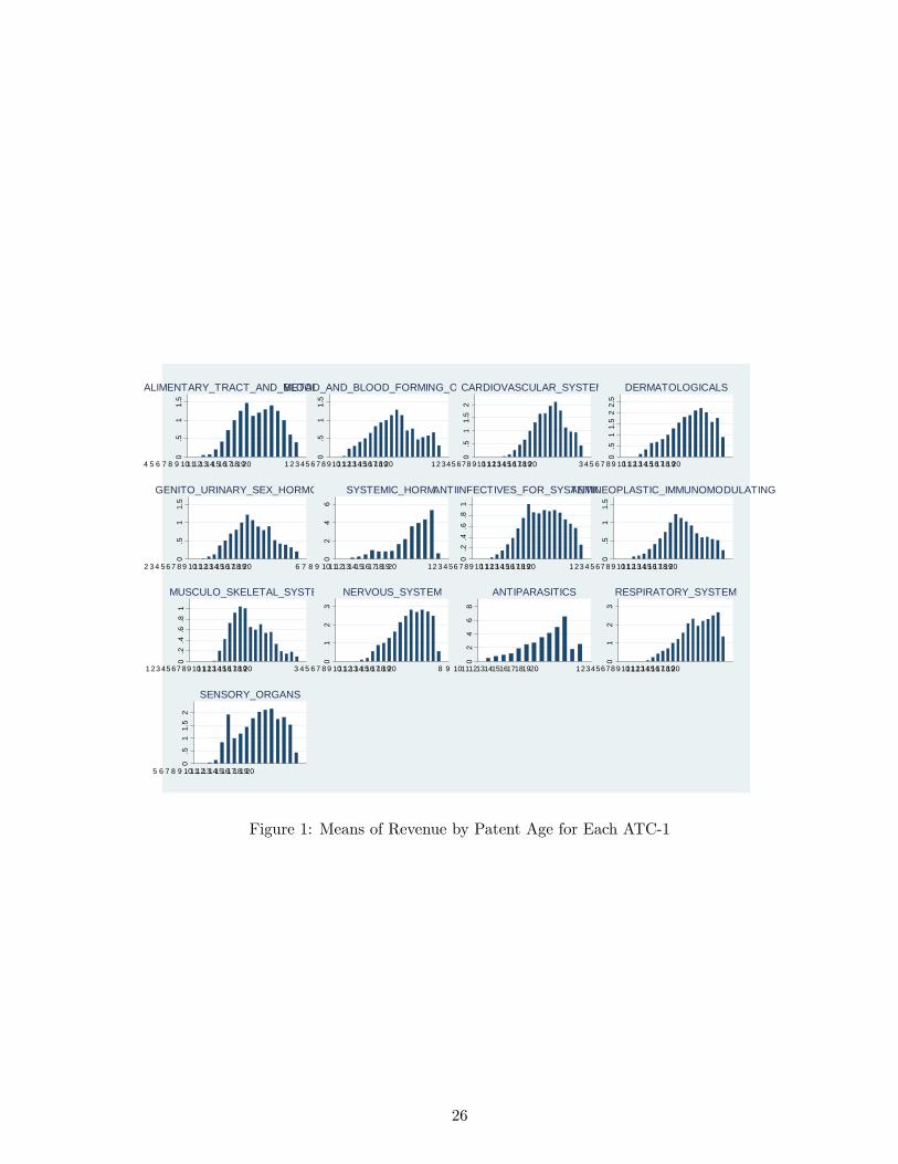
5.2 Lifecycle of drugs
In order to impute some unobserved revenues, we described above a method of imputation which
consists in estimating average lifecycle of drug revenues per ATC class. The estimation of these average
lifecycle of drugs is interesting and shown in next Figure 1 for all categories (digit 1 ATC classes) and
patent ages. Figure 1 shows the mean revenues of drugs by class for each patent age and ATC-1.
Remark that for these shapes to be seen on a same picture, we have normalized the total sales for
patent year 10 for all drug classes, which implies that the height of each vertical bar should not be
compared across drug categories.
We can see that the lifecycle of sales of drugs is not uniform across classes. Some classes have longer
delays of penetration, some classes have lower duration. These lifecycle shapes also show that sales
are not at all uniform during the patent life and thus that it seems important to take into account the
25
0.5
11.
5
4 5 6 7 8 9 1011121314151617181920
ALIMENTARY_TRACT_AND_METABOLISM
0.5
11.
5
1 2 3 45 6 7 8 91011121314151617181920
BLOOD_AND_BLOOD_FORMING_ORGANS
0.5
11.
52
12 345 678 91011121314151617181920
CARDIOVASCULAR_SYSTEM
0.5
11.
52
2.5
3 4 5 6 7 8 9 1011121314151617181920
DERMATOLOGICALS
0.5
11.
5
2 3 4 5 6 7 8 9 1011121314151617181920
GENITO_URINARY_SEX_HORMONES
02
46
6 7 8 9 1011121314151617181920
SYSTEMIC_HORM.
0.2
.4.6
.81
12 3 4 56 7 89 1011121314151617181920
ANTIINFECTIVES_FOR_SYSTEMIC_USE
0.5
11.
5
1 23 4 5 67 8 9 1011121314151617181920
ANTINEOPLASTIC_IMMUNOMODULATING
0.2
.4.6
.81
1 23 45 67 89 1011121314151617181920
MUSCULO_SKELETAL_SYSTEM
01
23
3 4 5 6 7 8 9 1011121314151617181920
NERVOUS_SYSTEM
02
46
8
8 9 1011121314151617181920
ANTIPARASITICS0
12
3
12345678 91011121314151617181920
RESPIRATORY_SYSTEM
0.5
11.
52
5 6 7 8 9 1011121314151617181920
SENSORY_ORGANS
Figure 1: Means of Revenue by Patent Age for Each ATC-1
26
0.5
11.
5
4 5 6 7 8 9 1011121314151617181920
ALIMENTARY_TRACT_AND_METABOLISM
0.2
.4.6
.81
1 2 3 45 6 7 8 91011121314151617181920
BLOOD_AND_BLOOD_FORMING_ORGANS
0.5
11.
5
12 345 678 91011121314151617181920
CARDIOVASCULAR_SYSTEM
0.5
11.
52
3 4 5 6 7 8 9 1011121314151617181920
DERMATOLOGICALS
0.2
.4.6
.81
2 3 4 5 6 7 8 9 1011121314151617181920
GENITO_URINARY_SEX_HORMONES
01
23
46 7 8 9 1011121314151617181920
SYSTEMIC_HORM.
0.5
11.
5
12 3 4 56 7 89 1011121314151617181920
ANTIINFECTIVES_FOR_SYSTEMIC_USE
0.2
.4.6
.81
1 23 4 5 67 8 9 1011121314151617181920
ANTINEOPLASTIC_IMMUNOMODULATING
0.2
.4.6
.81
1 23 45 67 89 1011121314151617181920
MUSCULO_SKELETAL_SYSTEM
0.5
11.
52
2.5
3 4 5 6 7 8 9 1011121314151617181920
NERVOUS_SYSTEM
02
46
8 9 1011121314151617181920
ANTIPARASITICS
0.5
11.
52
2.5
12345678 91011121314151617181920
RESPIRATORY_SYSTEM
0.5
11.
52
5 6 7 8 9 1011121314151617181920
SENSORY_ORGANS
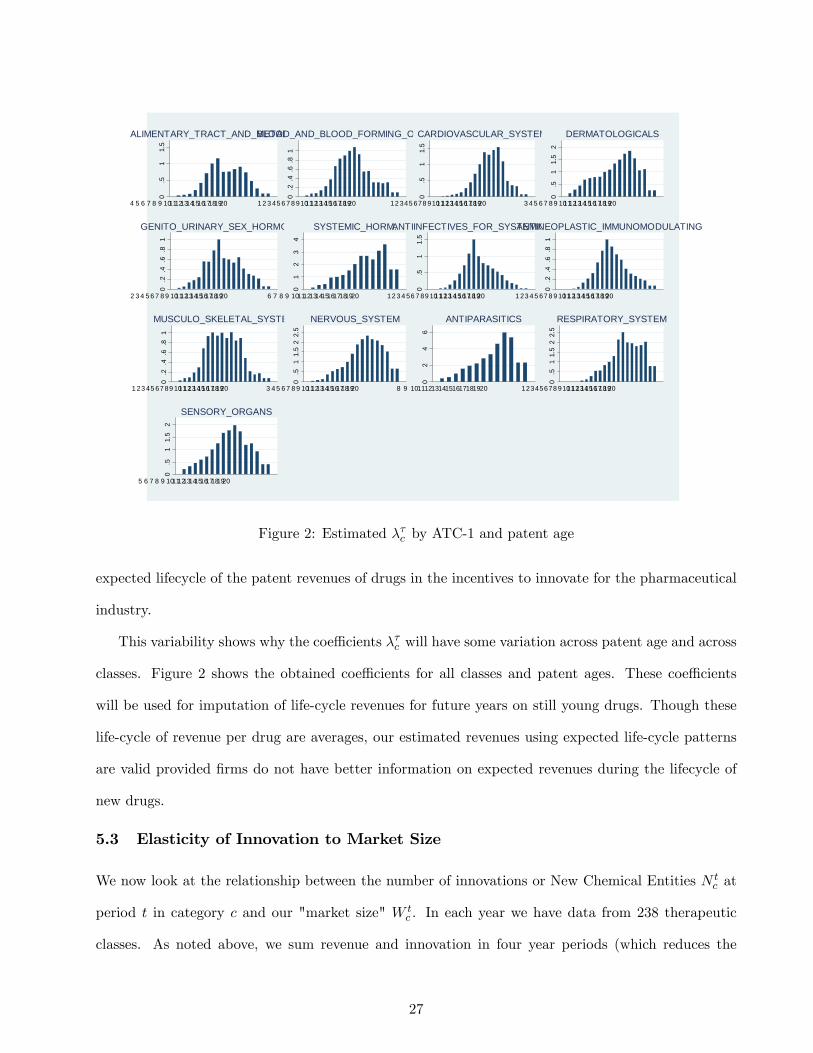
Figure 2: Estimated λτc by ATC-1 and patent age
expected lifecycle of the patent revenues of drugs in the incentives to innovate for the pharmaceutical
industry.
This variability shows why the coeffi cients λτc will have some variation across patent age and across
classes. Figure 2 shows the obtained coeffi cients for all classes and patent ages. These coeffi cients
will be used for imputation of life-cycle revenues for future years on still young drugs. Though these
life-cycle of revenue per drug are averages, our estimated revenues using expected life-cycle patterns
are valid provided firms do not have better information on expected revenues during the lifecycle of
new drugs.
5.3 Elasticity of Innovation to Market Size
We now look at the relationship between the number of innovations or New Chemical Entities N tc at
period t in category c and our "market size" W tc . In each year we have data from 238 therapeutic
classes. As noted above, we sum revenue and innovation in four year periods (which reduces the
27
sample size but creates much more content to each observation). Our time periods t are thus 1977-80,
1981-84, 1985-88, 1989-92, 1993-96, 1997-2000, 2001-04, 2005-2007.
We use several specifications to estimate the elasticity of innovation with respect to market size.
First, we estimate the following model
lnN tc = α lnW t
c + βc + δt + εtc
which relates the number of innovations (number of NCEs) patented in period t in each class to the
total revenue provided by sales of all drugs (on patent and licensed) in the class during the duration
of the patents issued at t.
In this reduced form model, α can be interpreted as the elasticity of innovation to market size, βc
is a fixed unobserved effect specific to the ATC class c, δt is a common unobserved period effect and
εtc an unobserved random shock on the innovation outcome.
Assuming all right hand side variables are exogenous means that
E(εtc| lnW t
c , βc, δt)
= 0
We first estimate such a model using OLS. Then we employ 2SLS because of the strong likelihood,
previously discussed, that innovation drives market size. Our instrumental variables are demographic:
population and mortality by disease (instead of prevalence which was not available) in different coun-
tries. To be valid instruments, demographics and disease mortality must be correlated with market
size. It is intuitive that the population and the share of the population likely to use drugs in each
ATC class will be correlated with the revenue in that class. Secondly, innovation, or launch of new
products, must not cause changes in demographics or disease mortality. We can imagine that at a
very fine level of categorization, this could be a problem. For example, a pill for Ausberger’s (mild
autism) might well increase diagnoses of Ausberger’s and therefore autism. But the WHO data we
use are much coarser: for example, how many people died of cardiovascular diseases in period t. We
do not think the therapies available for different cardiovascular diseases affect this measurement.
For this reason, we use male, female, and ”more than 50 years old”population variables, as well
as the number of deaths of males and females for the disease categories that each drug class (ATC
28
class) can be considered to target. This instrument is thus varying across periods and drug classes.
These set of instruments are interacted with dummy variables for 1-digit ATC classes or 2 digit ATC
classes depending on the cases.
For the population measures we compute the size of the population in countries where drugs of
each ATC class are sold and sum this over countries and years for the duration of the patent. This
population is denoted P ct . This instrument is varying not only over time but also across ATC classes.
We use a similar definition for male or female population, and for the ”over 50 years old”population.
Table 6 details the different sets of instruments used in the regressions below. As will be shown later,
these sets of instruments satisfy the different usual tests of exclusion (Sargan test of overidentifying
restrictions) and of significance in the first stage (F test of joint significance of excluded IVs in the
first stage regression). In our empirical work, set A will be used for regressions at the ATC-1 level
and B, C or D for regressions at the ATC-2 level.
Recall that the number of innovations N tc that can be observed on each market is censored at
zero, and that W tc is unobserved when there are zero innovations. We have a fundamental problem of
unobserved potential market size of any innovation that did not happen and therefore need a truncated
regression model. In particular, it could be that εtc is not mean independent of all right-hand-side
variables because of the truncation of the model when N tc = 0.
With some parametric assumptions on εtc, one can estimate the model taking into account the
truncation5. For example, as we are dealing with count data, we can assume a Poisson distribution
for the number of innovations, such that
P(N tc = n
)=
exp (−µ)µn
n!
where we specify the intensity parameter µ as µ = exp[αW t
c + βc + δt]. Such a model implies that
E(N tc |W t
c , βc, δt)
= exp[αW t
c + βc + δt]
As the data are truncated at zero sinceW tc is unobserved whenN
tc = 0, we correct for the truncation
5Nonparametric estimation of such a truncated regression model is diffi cult and is a subject of ongoing research (Lewbeland Linton, 2002, Chen 2009). Chen (2009) and Lewbel and Linton (2002) show that if the exogeneity assumption of righthand side variables is satisfied, then with some additional technical assumptions, one can identify the non parametricconditional expectation of the truncated dependent variable conditionally on the right hand side variables.
29

using the zero-truncated Poisson maximum-likelihood regression implying that
P(N tc = n|N t
c > 0)
=exp (−µ)µn
n! (1− exp (−µ))with µ = exp
[αW t
c + βc + δt]
In this case, we take into account the endogeneity ofW tc using a control function approach. As suggested
by Wooldridge (2002) and Blundell and Powell (2003), this technique is useful for non linear models.
It amounts to perform a first stage regression of the endogenous variables on all exogenous variables
and excluded instruments and then use residuals and polynomials of these residuals as additional
"control" variables in the main regression (here the zero-truncated Poisson). The results of this first
stage regressions6 show that excluded instruments are statistically significant (as confirmed also by the
joint F test shown at the bottom of the Tables). Results show that excluded IVs from sets A, B, C or D
are significant and the F test of joint significance always rejects strongly that they have no explanatory
power. In the case of the control function approaches, we used sets of instruments A for analysis of
N tc and D for N t
c′ but results are similar with other sets of instruments. In the case of ATC-1 level
regressions, instrumental variables A proved satisfactory and consist in male and female population
of corresponding countries, male and female deaths of corresponding ATC-1 class and countries. In
the case of ATC-2 level regressions, instrumental variables B, C or D proved satisfactory and consist
different male or female demographic variables interacted with ATC-1 or ATC-2 dummies.
In all following tables, standard errors are clustered at the class level and shown in parentheses.
Although dummy variables δt for time periods are not shown to conserve space, they are always
significant. Tables 7 and 8 show the results of estimating the linear model for the 1-digit and 2-digit
ATC categories respectively. Tables 9 and 10 show the corresponding results of the estimation of the
count models. In each case we show results with and without instrumenting for potential market size.
All standard errors are clustered at the ATC-1 level.
The specifications yield a range of elasticities between 6% and 40%, meaning that increasing
market size by 1% yields an increase in the number of new products of 0.06 to 0.4%. There is no clear
relationship between the elasticity and the type of specification (linear versus count, one-stage versus
two-stage) or the instrument set. Overall, our preferred specification among these is Equation (13).
6Available in additional online appendix available upon request in Table 14.
30
It takes into account the truncated nature of the data and the need to use instrumental variables,
and it uses the finer set of instruments in which the demographic variables are interacted with 2-digit
therapeutic categories, thus taking account of the fact that different demographic profiles generate
different market sizes in the various treatment categories. It uses the finer 2-digit disease classification
for the dependent variable, which we prefer because we understand it is relatively rare for drugs in
one ATC-2 category to be discovered while searching for therapies in a different ATC-2 category.
Equation (13) yields an elasticity of 12.3%, with a t-ratio of around 5, which gives the elasticity
a confidence interval of around 8% to 17%7. Given the assumptions of our model, this implies that
entry costs must be increasing in market size (since the marginal innovation requires substantially
higher revenue than the average innovation). Since we have no independent measure of quality we
cannot of course rule out the possibility that this is because the quality of pharmaceutical products
is increasing as market size increases. However, another interpretation is possible, which is that
innovation is subject to significant decreasing returns. This may be true both with respect to number
of innovations in a segment (the industry may be running out of "low-hanging fruit" - see Cowen
(2011)), and also true over time - the costs of regulatory approval appear to have been rising in recent
years. Although our results do not directly test the "low hanging fruit" hypothesis (because they
depend on the validity of our particular model of innovation) they are certainly compatible with it.
However, for this very reason the assumption that the elasticity is the same across disease categories
may not be realistic, since the extent to which the industry has had low-hanging fruit may well vary
for scientific reasons from one disease category to another. To investigate this possibility we estimate
the count model with ATC specific market size coeffi cients αc using
P(N tc = n|N t
c > 0)
=exp (−µ)µn
n! (1− exp (−µ))with µ = exp
[αcW
tc + βc + δt
]which also implies that the elasticity to market size of the expected number of innovations is ∂ lnENt
c∂ lnW t
c=
αcWtc .
Given the size of the elasticity, we can also compute how much additional revenue in a given drug
category is needed to obtain one additional innovation as the inverse of the elasticity times the average
7This point estimate enables us easily to reject the hypothesis of an elasticity equal to 1.
31
revenue per innovation observed on the market (because dWc =(∂ lnNc∂ lnWc
)−1WcNc)
Table 11 reports such results and Table 12 reports then the obtained elasticities by ATC class.
We find higher elasticities on average than in the model with the elasticity constrained to be constant
across disease categories, though they remain within the range of elasticities found under previous
specifications.
We see that the elasticities of innovation vary by ATC class, and that the average lifecycle dis-
counted market size increase needed on average to obtain one additional NCE also varies across
classes. For comparison, we estimate the log-linear model with ATC-1 specific elasticities (results not
reported), and find larger absolute values than in a specification without heterogeneity. The values
are a little smaller than those of this count model, varying between 8% and 30% depending on the
disease class.
Across all ATC classes, we find that the average elasticity of innovation to market size under this
specification is 25.2%, which implies that the average lifecycle discounted market size increase needed
to obtain one additional NCE is around $1.8 billion. Remember that we used a discount factor of
0.95 which implies that the $1.8 billion over the lifecycle of a drug is equivalent to a constant annual
revenue of $148 million per year over 20 years.
Next we consider whether this estimated $1.8 billion is reasonable. The most recent DiMasi et al.
study of drug development estimates that a new drug incurs approximately $800 million in development
costs (Adams, 2006, Di Masi et al. 2003 suggest 1$billion on average for one new chemical entity).
Included in this calculation is the cost of capital, the cost of failed drugs, and the cost of clinical trials,
so it is close to the total fixed economic cost of innovation. On top of this there will be variable costs
of production, distribution and marketing. Industry sources have suggested to us that 50% of revenue
is a reasonable guess at the size of these costs (though they may be higher in the case of biologics,
where manufacturing costs are typically higher). This suggests that a new drug would need to cover
costs of around $1.6 billion in order to yield a return to the innovator. This is a little lower than our
estimated market size increase of $1.8 billion needed to induce an additional innovation. Our elasticity
estimate therefore seems broadly plausible in the light of what is known from accounting data.
32
Comparing our elasticities to others in the literature is diffi cult, if only because the dependent
variable changes across research designs from new drugs, to new cancer regimens, to new clinical trials,
to journal articles. However, both AL and we use new product launch as a measure of innovation.
Recall that AL estimate an elasticity of 4: for each 1% increase in revenue, the number of new products
increases by 4%, which is over an order of magnitude larger than our estimate (and of most others in
the literature). There are significant empirical differences that underlie these two different results. For
example, all new products including new forms, strengths, and generic versions are counted in the AL
methodology. The authors include only US revenue in their measure of market size. Lastly, as noted
above, the method in AL does not include an instrument for market size. Though it is hard to know
the impact of these methodological differences (explained in Appendix 7.1), an elasticity as large as 4
appears to imply that marginal costs of innovation are falling as more innovation takes place, which
does not seem a plausible description of the pharmaceutical industry in the early 21st century.
6 Conclusion
This paper has attempted to quantify the relationship between market size and innovation in the
pharmaceutical industry. We have estimated the elasticity of innovation (as measured by the number
of new chemical entities appearing on the market for a given disease class) to the expected market
size, which is predictable by the potential demand as represented by the willingness of sufferers from
diseases in a class (and others acting on their behalf such as insurers or governments) to spend on their
treatment. We have found significant positive elasticities with a point estimate under our preferred
specification of 25.2%. This suggests that at the mean market size an additional $1.8 billion is required
in additional revenue to induce the invention of one additional new chemical entity, which appears a
reasonable order of magnitude since estimates of the true economic cost of developing a new chemical
entity are around $800 million to $1 billion, and marketing and related costs represent some 50% of
revenue. An elasticity substantially below one is also plausible in the light of other evidence that
innovation in pharmaceuticals is becoming more diffi cult and expensive over time, and is compatible
both with the hypothesis that the costs of regulatory approval are rising and the hypothesis that the
33

industry is running out of ”low hanging fruit.”
Our results are robust to a number of specification choices. However, the availability of data for
more years would undoubtedly help to refine our estimates and we leave this as a subject for future
research.
34
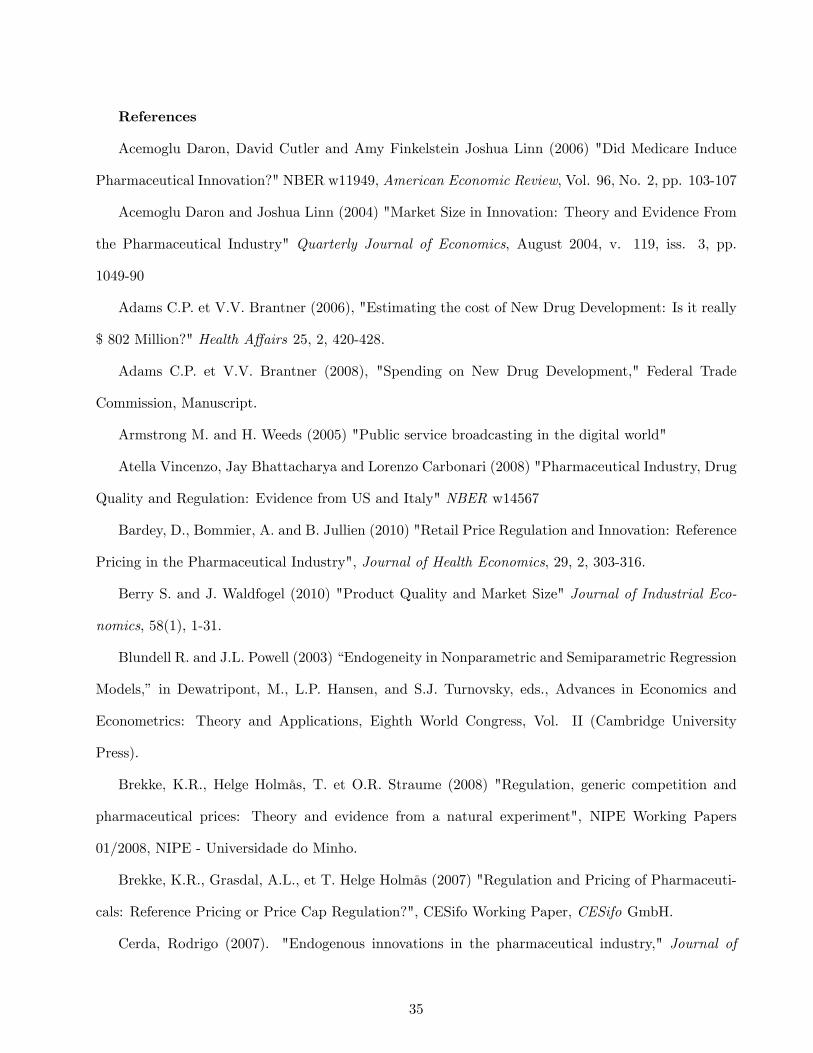
References
Acemoglu Daron, David Cutler and Amy Finkelstein Joshua Linn (2006) "Did Medicare Induce
Pharmaceutical Innovation?" NBER w11949, American Economic Review, Vol. 96, No. 2, pp. 103-107
Acemoglu Daron and Joshua Linn (2004) "Market Size in Innovation: Theory and Evidence From
the Pharmaceutical Industry" Quarterly Journal of Economics, August 2004, v. 119, iss. 3, pp.
1049-90
Adams C.P. et V.V. Brantner (2006), "Estimating the cost of New Drug Development: Is it really
$ 802 Million?" Health Affairs 25, 2, 420-428.
Adams C.P. et V.V. Brantner (2008), "Spending on New Drug Development," Federal Trade
Commission, Manuscript.
Armstrong M. and H. Weeds (2005) "Public service broadcasting in the digital world"
Atella Vincenzo, Jay Bhattacharya and Lorenzo Carbonari (2008) "Pharmaceutical Industry, Drug
Quality and Regulation: Evidence from US and Italy" NBER w14567
Bardey, D., Bommier, A. and B. Jullien (2010) "Retail Price Regulation and Innovation: Reference
Pricing in the Pharmaceutical Industry", Journal of Health Economics, 29, 2, 303-316.
Berry S. and J. Waldfogel (2010) "Product Quality and Market Size" Journal of Industrial Eco-
nomics, 58(1), 1-31.
Blundell R. and J.L. Powell (2003) “Endogeneity in Nonparametric and Semiparametric Regression
Models,” in Dewatripont, M., L.P. Hansen, and S.J. Turnovsky, eds., Advances in Economics and
Econometrics: Theory and Applications, Eighth World Congress, Vol. II (Cambridge University
Press).
Brekke, K.R., Helge Holmås, T. et O.R. Straume (2008) "Regulation, generic competition and
pharmaceutical prices: Theory and evidence from a natural experiment", NIPE Working Papers
01/2008, NIPE - Universidade do Minho.
Brekke, K.R., Grasdal, A.L., et T. Helge Holmås (2007) "Regulation and Pricing of Pharmaceuti-
cals: Reference Pricing or Price Cap Regulation?", CESifo Working Paper, CESifo GmbH.
Cerda, Rodrigo (2007). "Endogenous innovations in the pharmaceutical industry," Journal of
35

Evolutionary Economics, Springer, vol. 17(4), pages 473-515
Chaudhuri Shubham, Pinelopi K. Goldberg and Panle Jia (2003) "Estimating the Effects of Global
Patent Protection in Pharmaceuticals: A Case Study of Quinolones in India" NBER w10159
Civan, Abdulkadir and Michael Maloney, (2006a) "The Effect of Price on Pharmaceutical R&D",
Berkeley Electronic Press, Contributions to Economic Analysis and Policy, Vol. 5, Iss. 1, art. 28
Civan, Abdulkadir and Michael Maloney, (2006b) "The Effect of Price on Pharmaceutical R&D"
http://myweb.clemson.edu/~maloney/papers/DrugPrices-and-Development.pdf
Cowen, Tyler, (2011) The Great Stagnation. New York, Penguin Press, E-book.
Congressional Budget Offi ce (2006) "Research and Development in the Pharmaceutical Industry",
Congress of the United States
Danzon, P.M and H. Lui (1996) "RP and physician drug budgets: the German experience in
controlling health expenditure", Working Paper, The Wharton School.
Danzon, P.M et J.D. Ketcham (2004) Reference pricing of pharmaceuticals for medicare: Evidence
from Germany and New Zealand. Frontiers in Health Policy Research, vol. 7, Cutler, D.M. et A.M.
Garber (eds) NBER and MIT Press.
Danzon P. and M. Furukawa (2006) "Prices And Availability Of Biopharmaceuticals: An Interna-
tional Comparison" Health Affairs, 25, 5, 1353-1362
Danzon Patricia, Richard Wang and Liang Wang (2005) "The impact of price regulation on the
launch delay of new drugs evidence from twenty-major markets in the1990s" Health Economics 14(3):
269—292
DiMasi, J.A., Hansen, R.W., Grabowski, H.G. et L. Lasagna (1991) "Cost of innovation in the
pharmaceutical industry", Journal of Health Economics 10, 107-142.
DiMasi, J.A., Hansen, R.W. et H.G. Grabowski (2003) "The price of innovation: New estimates
of Drug Development Costs", Journal of Health Economics 22, 151-185.
Duggan Mark and Fiona Scott Morton (2008) "The Effect of Medicare Part D on Pharmaceutical
Prices and Utilization" NBER w13917
Ellison Glenn and Sara Fisher Ellison (2007) "Strategic Entry Deterrence and the Behavior of
36

Pharmaceutical Incumbents Prior to Patent Expiration" NBER w13069
Finkelstein, Amy (2004) "Static and Dynamic Effects of Health Policy: Evidence from the Vaccine
Industry", Quarterly Journal of Economics 119(2): 527-564
Golec, J.H., et J.A. Vernon (2006) European pharmaceutical price regulation, firm profitability
and R&D spending, NBER Working Paper 12676.
Lewbel A. and O. Linton (2002) "Nonparametric Censored and Truncated Regression" Economet-
rica (2002) 70, 765-779
Lichtenberg Frank R. and Gautier Duflos (2008) "Pharmaceutical innovation and the longevity of
Australians: a first look" NBER wp 14009
Lichtenberg, F., (2005), "Pharmaceutical innovation and the burden of disease in developing and
developed countries," Journal of Medicine and Philosophy 30(6), December 2005.
Mullahy, John. (1997) "Instrumental-Variable Estimation of Count Data Models: Applications to
Models of Cigarette Smoking Behavior." The Review of Economics and Statistics, 79(4):586-593.
Sutton J. (1991) Sunk Costs and Market Structure, MIT Press
Vernon, J. (2005) "Examining the link between price regulation and pharmaceutical R&D Invest-
ment", Health Economics 14, 1-16.
Wooldridge J. M. (2002) Econometric Analysis of Cross Section and Panel Data. MIT Press
Yin, Wesley (2009) "R&D Policy, Agency Costs and Innovation in Personalized Medicine", Journal
of Health Economics, 28(5), pp. 950-962
Yin, Wesley (2008) "Market Incentives and Pharmaceutical Innovation", Journal of Health Eco-
nomics, July 2008, 27(4), pp. 1060-1077
37

7 Appendix
7.1 Analysis of Elasticity to Contemporaneous Revenue
Suppose we assume instead that lnN tc = αW t
c . In this case we would want to know the bias that comes
from using the contemporaneous revenue R rather than W . In our empirical work, this amounts to
study the derivative of E(lnN t
c |Rtc)with respect to Rtc. Then,
lnN tc = α
∑{d∈c,t0a=t}
R̃d = α∑
{d∈c,t0d=t}
t0d+20∑t′=t0d
δt′−t0dRt
′d
= α
∑{d∈c,t0d=t}
Rtd
+ α
∑{d∈c,t0d=t}
t0d+20∑t′=t+1
δt′−t0dRt
′d
= αRtc − α
∑t′<t
∑{d∈c,t0d=t′}
Rtd
+ α
∑{d∈c,t0d=t}
t0d+20∑t′=t+1
δt′−t0dRt
′d
because Rtc =
∑{d∈c}R
td =
∑t′<t
∑{d∈c,t0d=t′}R
td +
∑{d∈c,t0d=t}R
td.
Then
E(lnN t
c |Rtc)
= αRtc − αE
∑t′<t
∑{d∈c,t0d=t′}
Rtd
∣∣∣∣∣∣∣Rtc+ αE
∑{d∈c,t0d=t}
t0d+20∑t′=t+1
δt′−t0dRt
′d
∣∣∣∣∣∣∣Rtc
and both E(∑
t′<t
∑{d∈c,t0d=t′}R
td
∣∣∣Rtc) and E(∑{d∈c,t0d=t}
∑t0d+20
t′=t+1 δt′−t0dRt
′d
∣∣∣Rtc) have no reasonto be zero if there is some correlation between revenues for the same drug across periods (which is
obviously the case). Remark that if revenues per drug are all independent and that we only have time
autocorrelation of revenues then both terms should be positive and thus E(lnN t
c |Rtc)could be either
higher or lower than αRtc.
If for example the revenues of a drug d in year t and t0d are proportional to a scale factor depending
only on the class to which it belongs to and the patent age t− t0d, then Rtd = λt−t0dc R
t0dc and
E(lnN t
c |Rtc)
= αRtc
1 +
∑{d∈c,t0d=t}
t0d+20∑t′=t+1
δt′−t0dλ
t′−t0dc
− αE
∑t′<t
∑{d∈c,t0d=t′}
Rtd
∣∣∣∣∣∣∣Rtc
where∑{d∈c,t0d=t}
∑t0d+20
t′=t+1 δt′−t0dλ
t′−t0dc would be equal to 20 if revenues are constant per drug during
the patent life and there is no discounting. Thus, unless E(∑
t′<t
∑{d∈c,t0d=t′}R
td
∣∣∣Rtc) is also positiveand very large,
∂E(lnNtc |Rtc)
∂Rtcwould be much larger than α.
38
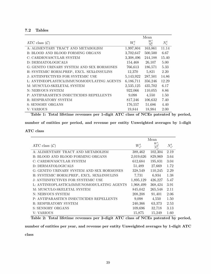
7.2 Tables
Mean
ATC class (C) W tc
W tc
Ntc
N tc
A: ALIMENTARY TRACT AND METABOLISM 1,997,804 163,861 11.14B: BLOOD AND BLOOD FORMING ORGANS 3,702,647 500,500 6.67C: CARDIOVASCULAR SYSTEM 3,308,496 244,188 15.40D: DERMATOLOGICALS 154,468 26,107 5.00G: GENITO URINARY SYSTEM AND SEX HORMONES 766,613 186,571 5.33H: SYSTEMIC HORM.PREP., EXCL. SEX&INSULINS 12,370 5,821 2.20J: ANTIINFECTIVES FOR SYSTEMIC USE 5,143,922 287,501 14.86L: ANTINEOPLASTIC&IMMUNOMODULATING AGENTS 6,186,711 356,246 12.29M: MUSCULO-SKELETAL SYSTEM 2,535,125 435,702 6.17N: NERVOUS SYSTEM 922,066 110,055 8.86P: ANTIPARASITICS INSECTICIDES REPELLENTS 9,098 4,550 1.50R: RESPIRATORY SYSTEM 817,246 106,632 7.40S: SENSORY ORGANS 176,557 51,686 4.40V: VARIOUS 19,844 18,984 2.00Table 1: Total lifetime revenues per 1-digit ATC class of NCEs patented by period,
number of entities per period, and revenue per entity Unweighted averages by 1-digit
ATC class
Mean
ATC class (C) W tc′
W tc′
Ntc′
N tc′
A: ALIMENTARY TRACT AND METABOLISM 388,462 102,304 2.19B: BLOOD AND BLOOD FORMING ORGANS 2,019,626 829,969 3.64C: CARDIOVASCULAR SYSTEM 612,684 195,831 3.04D: DERMATOLOGICALS 51,489 27,669 1.72G: GENITO URINARY SYSTEM AND SEX HORMONES 328,549 110,245 2.29H: SYSTEMIC HORM.PREP., EXCL. SEX&INSULINS 7,731 6,934 1.38J: ANTIINFECTIVES FOR SYSTEMIC USE 1,895,129 426,227 5.47L: ANTINEOPLASTIC&IMMUNOMODULATING AGENTS 1,968,499 368,424 3.91M: MUSCULO-SKELETAL SYSTEM 845,042 265,548 2.11N: NERVOUS SYSTEM 208,208 91,401 2.06P: ANTIPARASITICS INSECTICIDES REPELLENTS 9,098 4,550 1.50R: RESPIRATORY SYSTEM 240,366 63,373 2.53S: SENSORY ORGANS 109,696 32,718 3.13V: VARIOUS 15,875 15,249 1.60Table 2: Total lifetime revenues per 2-digit ATC class of NCEs patented by period,
number of entities per year, and revenue per entity Unweighted averages by 1-digit ATC
class
39
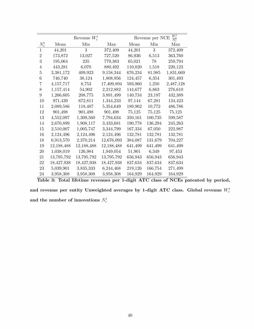
Revenue W tc Revenue per NCE W t
cNtc
N tc Mean Min Max Mean Min Max
1 44,201 3 372,409 44,201 3 372,4092 173,872 13,027 727,520 86,936 6,513 363,7603 195,064 235 779,383 65,021 78 259,7944 443,281 6,070 880,492 110,820 1,518 220,1235 3,381,172 409,923 9,158,344 676,234 81,985 1,831,6696 746,740 38,124 1,808,956 124,457 6,354 301,4937 4,157,717 8,753 17,409,894 593,960 1,250 2,487,1288 1,157,414 54,902 2,212,882 144,677 6,863 276,6109 1,266,605 208,775 3,891,499 140,734 23,197 432,38910 971,439 672,811 1,344,233 97,144 67,281 134,42311 2,089,586 118,487 5,354,649 189,962 10,772 486,78612 901,498 901,498 901,498 75,125 75,125 75,12513 4,552,097 1,309,560 7,794,634 350,161 100,735 599,58714 2,670,899 1,908,117 3,433,681 190,778 136,294 245,26315 2,510,007 1,005,747 3,344,799 167,334 67,050 222,98716 2,124,496 2,124,496 2,124,496 132,781 132,781 132,78118 6,913,570 2,370,214 12,676,093 384,087 131,679 704,22719 12,188,488 12,188,488 12,188,488 641,499 641,499 641,49920 1,038,019 126,984 1,949,054 51,901 6,349 97,45321 13,795,792 13,795,792 13,795,792 656,943 656,943 656,94322 18,427,938 18,427,938 18,427,938 837,634 837,634 837,63423 5,039,901 3,835,333 6,244,468 219,126 166,754 271,49924 3,958,308 3,958,308 3,958,308 164,929 164,929 164,929Table 3: Total lifetime revenues per 1-digit ATC class of NCEs patented by period,
and revenue per entity Unweighted averages by 1-digit ATC class. Global revenue W tc
and the number of innovations N tc
40
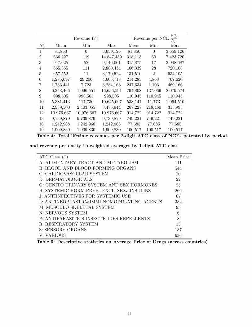
Revenue W tc′ Revenue per NCE
W tc′
Ntc′
N tc′ Mean Min Max Mean Min Max
1 81,850 0 3,659,126 81,850 0 3,659,1262 636,227 119 14,847,439 318,113 60 7,423,7203 947,625 52 9,146,061 315,875 17 3,048,6874 665,355 111 2,880,434 166,339 28 720,1085 657,552 11 3,170,524 131,510 2 634,1056 1,285,697 29,206 4,605,718 214,283 4,868 767,6207 1,733,441 7,723 3,284,163 247,634 1,103 469,1668 6,358,466 1,096,551 16,636,591 794,808 137,069 2,079,5749 998,505 998,505 998,505 110,945 110,945 110,94510 5,381,413 117,730 10,645,097 538,141 11,773 1,064,51011 2,939,500 2,403,055 3,475,944 267,227 218,460 315,99512 10,976,667 10,976,667 10,976,667 914,722 914,722 914,72213 9,739,879 9,739,879 9,739,879 749,221 749,221 749,22116 1,242,968 1,242,968 1,242,968 77,685 77,685 77,68519 1,909,830 1,909,830 1,909,830 100,517 100,517 100,517Table 4: Total lifetime revenues per 2-digit ATC class of NCEs patented by period,
and revenue per entity Unweighted averages by 1-digit ATC class
ATC Class (C) Mean PriceA: ALIMENTARY TRACT AND METABOLISM 111B: BLOOD AND BLOOD FORMING ORGANS 544C: CARDIOVASCULAR SYSTEM 10D: DERMATOLOGICALS 22G: GENITO URINARY SYSTEM AND SEX HORMONES 23H: SYSTEMIC HORM.PREP., EXCL. SEX&INSULINS 266J: ANTIINFECTIVES FOR SYSTEMIC USE 67L: ANTINEOPLASTIC&IMMUNOMODULATING AGENTS 382M: MUSCULO-SKELETAL SYSTEM 95N: NERVOUS SYSTEM 6P: ANTIPARASITICS INSECTICIDES REPELLENTS 8R: RESPIRATORY SYSTEM 13S: SENSORY ORGANS 187V: VARIOUS 636
Table 5: Descriptive statistics on Average Price of Drugs (across countries)
41
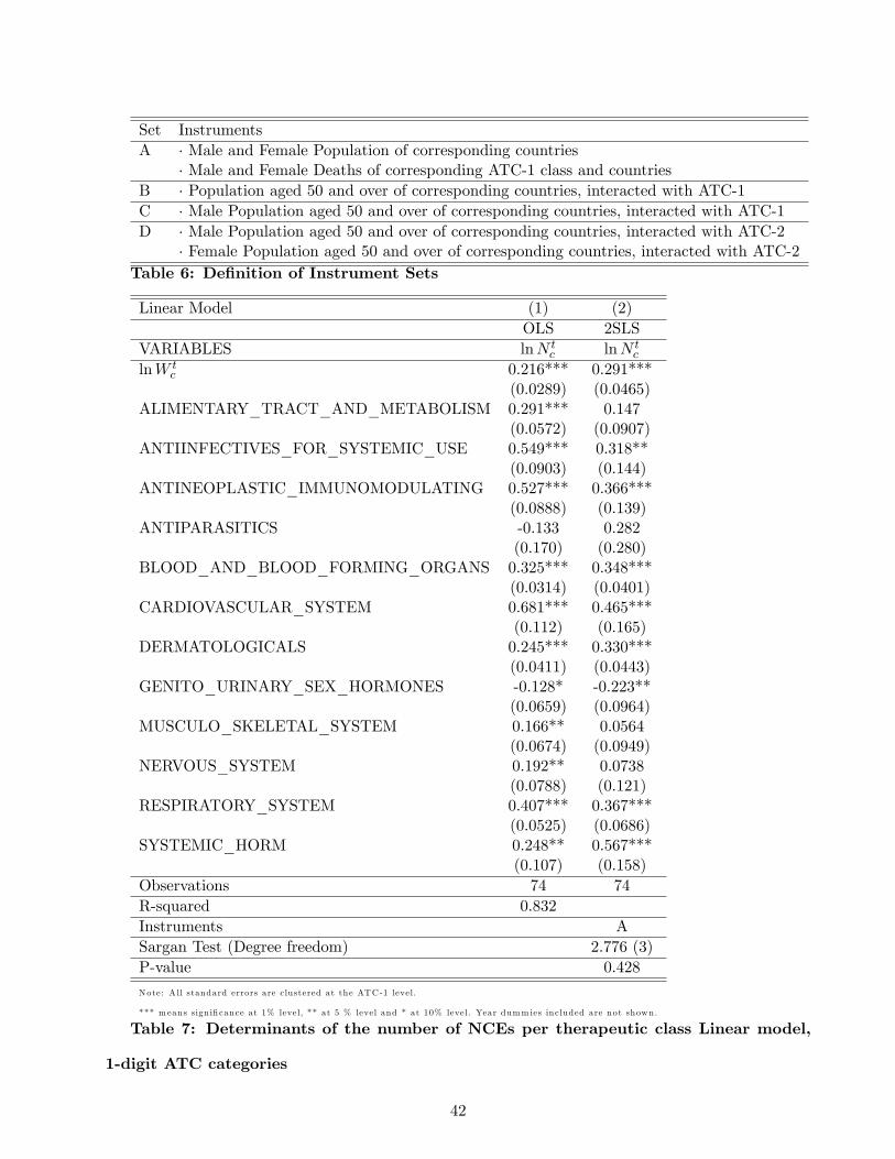
Set InstrumentsA · Male and Female Population of corresponding countries
· Male and Female Deaths of corresponding ATC-1 class and countriesB · Population aged 50 and over of corresponding countries, interacted with ATC-1C · Male Population aged 50 and over of corresponding countries, interacted with ATC-1D · Male Population aged 50 and over of corresponding countries, interacted with ATC-2
· Female Population aged 50 and over of corresponding countries, interacted with ATC-2Table 6: Definition of Instrument Sets
Linear Model (1) (2)OLS 2SLS
VARIABLES lnN tc lnN t
c
lnW tc 0.216*** 0.291***
(0.0289) (0.0465)ALIMENTARY_TRACT_AND_METABOLISM 0.291*** 0.147
(0.0572) (0.0907)ANTIINFECTIVES_FOR_SYSTEMIC_USE 0.549*** 0.318**
(0.0903) (0.144)ANTINEOPLASTIC_IMMUNOMODULATING 0.527*** 0.366***
(0.0888) (0.139)ANTIPARASITICS -0.133 0.282
(0.170) (0.280)BLOOD_AND_BLOOD_FORMING_ORGANS 0.325*** 0.348***
(0.0314) (0.0401)CARDIOVASCULAR_SYSTEM 0.681*** 0.465***
(0.112) (0.165)DERMATOLOGICALS 0.245*** 0.330***
(0.0411) (0.0443)GENITO_URINARY_SEX_HORMONES -0.128* -0.223**
(0.0659) (0.0964)MUSCULO_SKELETAL_SYSTEM 0.166** 0.0564
(0.0674) (0.0949)NERVOUS_SYSTEM 0.192** 0.0738
(0.0788) (0.121)RESPIRATORY_SYSTEM 0.407*** 0.367***
(0.0525) (0.0686)SYSTEMIC_HORM 0.248** 0.567***
(0.107) (0.158)Observations 74 74R-squared 0.832Instruments ASargan Test (Degree freedom) 2.776 (3)P-value 0.428
Note: A ll standard errors are clustered at the ATC-1 level.
*** m eans sign ificance at 1% level, ** at 5 % level and * at 10% level. Year dumm ies included are not shown.
Table 7: Determinants of the number of NCEs per therapeutic class Linear model,
1-digit ATC categories
42
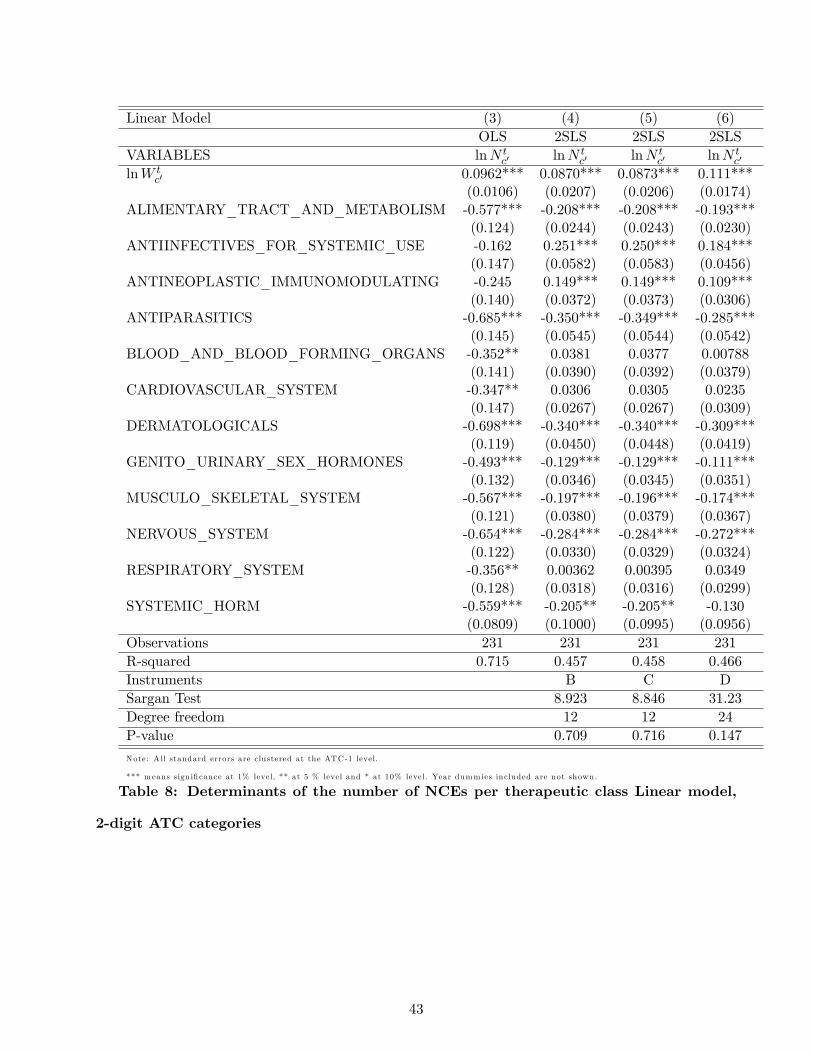
Linear Model (3) (4) (5) (6)OLS 2SLS 2SLS 2SLS
VARIABLES lnN tc′ lnN t
c′ lnN tc′ lnN t
c′
lnW tc′ 0.0962*** 0.0870*** 0.0873*** 0.111***
(0.0106) (0.0207) (0.0206) (0.0174)ALIMENTARY_TRACT_AND_METABOLISM -0.577*** -0.208*** -0.208*** -0.193***
(0.124) (0.0244) (0.0243) (0.0230)ANTIINFECTIVES_FOR_SYSTEMIC_USE -0.162 0.251*** 0.250*** 0.184***
(0.147) (0.0582) (0.0583) (0.0456)ANTINEOPLASTIC_IMMUNOMODULATING -0.245 0.149*** 0.149*** 0.109***
(0.140) (0.0372) (0.0373) (0.0306)ANTIPARASITICS -0.685*** -0.350*** -0.349*** -0.285***
(0.145) (0.0545) (0.0544) (0.0542)BLOOD_AND_BLOOD_FORMING_ORGANS -0.352** 0.0381 0.0377 0.00788
(0.141) (0.0390) (0.0392) (0.0379)CARDIOVASCULAR_SYSTEM -0.347** 0.0306 0.0305 0.0235
(0.147) (0.0267) (0.0267) (0.0309)DERMATOLOGICALS -0.698*** -0.340*** -0.340*** -0.309***
(0.119) (0.0450) (0.0448) (0.0419)GENITO_URINARY_SEX_HORMONES -0.493*** -0.129*** -0.129*** -0.111***
(0.132) (0.0346) (0.0345) (0.0351)MUSCULO_SKELETAL_SYSTEM -0.567*** -0.197*** -0.196*** -0.174***
(0.121) (0.0380) (0.0379) (0.0367)NERVOUS_SYSTEM -0.654*** -0.284*** -0.284*** -0.272***
(0.122) (0.0330) (0.0329) (0.0324)RESPIRATORY_SYSTEM -0.356** 0.00362 0.00395 0.0349
(0.128) (0.0318) (0.0316) (0.0299)SYSTEMIC_HORM -0.559*** -0.205** -0.205** -0.130
(0.0809) (0.1000) (0.0995) (0.0956)Observations 231 231 231 231R-squared 0.715 0.457 0.458 0.466Instruments B C DSargan Test 8.923 8.846 31.23Degree freedom 12 12 24P-value 0.709 0.716 0.147
Note: A ll standard errors are clustered at the ATC-1 level.
*** m eans sign ificance at 1% level, ** at 5 % level and * at 10% level. Year dumm ies included are not shown.
Table 8: Determinants of the number of NCEs per therapeutic class Linear model,
2-digit ATC categories
43
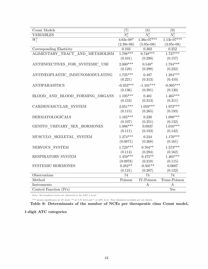
Count Models (7) (8) (9)VARIABLES N t
c N tc N t
c
W tc 4.63e-08* 1.36e-07*** 1.13e-07***
(2.39e-08) (5.05e-08) (3.05e-08)Corresponding Elasticity 0.103 0.303 0.252ALIMENTARY_TRACT_AND_METABOLISM 1.798*** 0.748*** 1.727***
(0.101) (0.290) (0.157)
ANTIINFECTIVES_FOR_SYSTEMIC_USE 2.000*** 0.548* 1.784***(0.128) (0.298) (0.232)
ANTINEOPLASTIC_IMMUNOMODULATING 1.725*** 0.487 1.284***(0.221) (0.313) (0.410)
ANTIPARASITICS -0.353*** -1.101*** -0.905***(0.136) (0.391) (0.130)
BLOOD_AND_BLOOD_FORMING_ORGANS 1.195*** 0.401 1.465***(0.153) (0.313) (0.211)
CARDIOVASCULAR_SYSTEM 2.051*** 1.059*** 1.972***(0.115) (0.265) (0.193)
DERMATOLOGICALS 1.165*** 0.230 1.098***(0.107) (0.251) (0.132)
GENITO_URINARY_SEX_HORMONES 1.086*** 0.0937 1.010***(0.111) (0.183) (0.142)
MUSCULO_SKELETAL_SYSTEM 1.274*** 0.234 1.170***(0.0871) (0.268) (0.161)
NERVOUS_SYSTEM 1.723*** 0.704** 1.573***(0.114) (0.294) (0.162)
RESPIRATORY SYSTEM 1.459*** 0.475** 1.465***(0.0978) (0.210) (0.115)
SYSTEMIC HORMONES 0.282** -0.501** 0.0607(0.121) (0.207) (0.122)
Observations 74 74 74Method Poisson IV-Poisson Trunc-PoissonInstruments A AControl Function (IVs) Yes
Note: A ll standard errors are clustered at the ATC-1 level.
*** m eans sign ificance at 1% level, ** at 5 % level and * at 10% level. Year dumm ies included are not shown.
Table 9: Determinants of the number of NCEs per therapeutic class Count model,
1-digit ATC categories
44
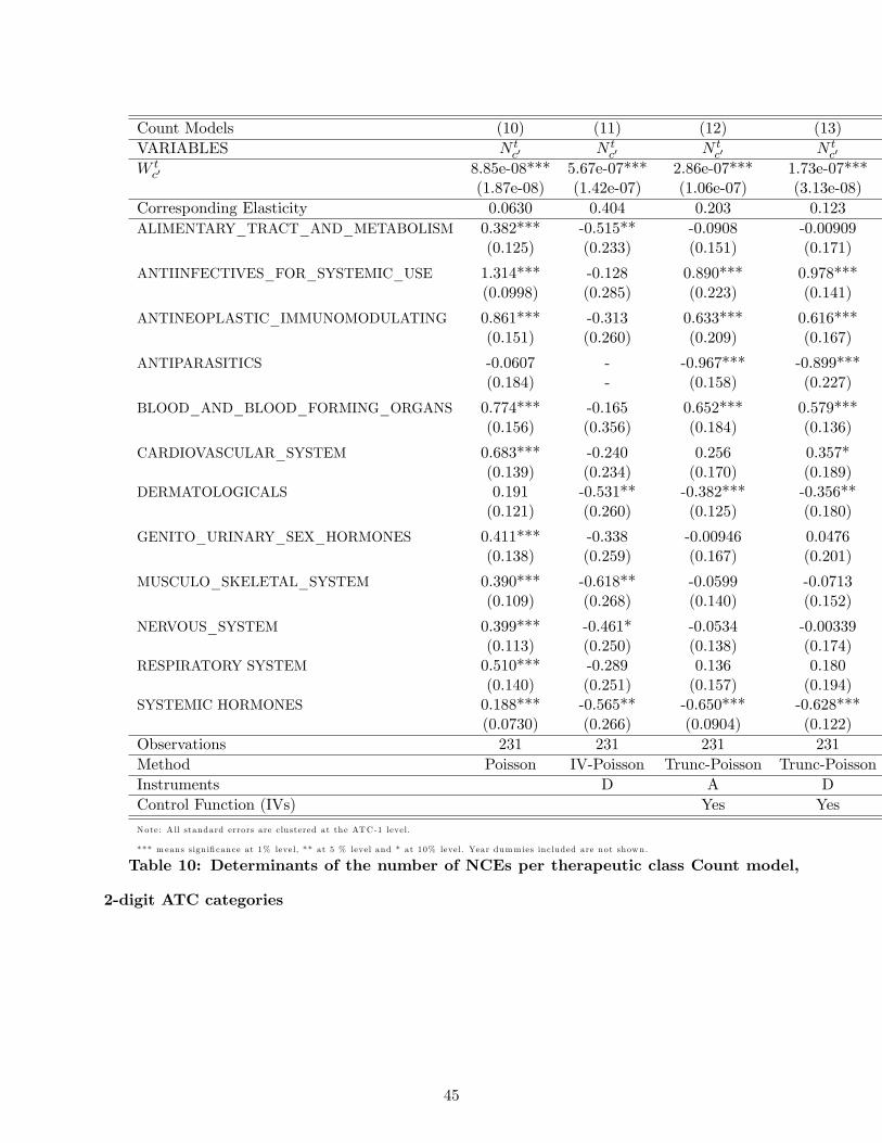
Count Models (10) (11) (12) (13)VARIABLES N t
c′ N tc′ N t
c′ N tc′
W tc′ 8.85e-08*** 5.67e-07*** 2.86e-07*** 1.73e-07***
(1.87e-08) (1.42e-07) (1.06e-07) (3.13e-08)Corresponding Elasticity 0.0630 0.404 0.203 0.123ALIMENTARY_TRACT_AND_METABOLISM 0.382*** -0.515** -0.0908 -0.00909
(0.125) (0.233) (0.151) (0.171)
ANTIINFECTIVES_FOR_SYSTEMIC_USE 1.314*** -0.128 0.890*** 0.978***(0.0998) (0.285) (0.223) (0.141)
ANTINEOPLASTIC_IMMUNOMODULATING 0.861*** -0.313 0.633*** 0.616***(0.151) (0.260) (0.209) (0.167)
ANTIPARASITICS -0.0607 - -0.967*** -0.899***(0.184) - (0.158) (0.227)
BLOOD_AND_BLOOD_FORMING_ORGANS 0.774*** -0.165 0.652*** 0.579***(0.156) (0.356) (0.184) (0.136)
CARDIOVASCULAR_SYSTEM 0.683*** -0.240 0.256 0.357*(0.139) (0.234) (0.170) (0.189)
DERMATOLOGICALS 0.191 -0.531** -0.382*** -0.356**(0.121) (0.260) (0.125) (0.180)
GENITO_URINARY_SEX_HORMONES 0.411*** -0.338 -0.00946 0.0476(0.138) (0.259) (0.167) (0.201)
MUSCULO_SKELETAL_SYSTEM 0.390*** -0.618** -0.0599 -0.0713(0.109) (0.268) (0.140) (0.152)
NERVOUS_SYSTEM 0.399*** -0.461* -0.0534 -0.00339(0.113) (0.250) (0.138) (0.174)
RESPIRATORY SYSTEM 0.510*** -0.289 0.136 0.180(0.140) (0.251) (0.157) (0.194)
SYSTEMIC HORMONES 0.188*** -0.565** -0.650*** -0.628***(0.0730) (0.266) (0.0904) (0.122)
Observations 231 231 231 231Method Poisson IV-Poisson Trunc-Poisson Trunc-PoissonInstruments D A DControl Function (IVs) Yes Yes
Note: A ll standard errors are clustered at the ATC-1 level.
*** m eans sign ificance at 1% level, ** at 5 % level and * at 10% level. Year dumm ies included are not shown.
Table 10: Determinants of the number of NCEs per therapeutic class Count model,
2-digit ATC categories
45
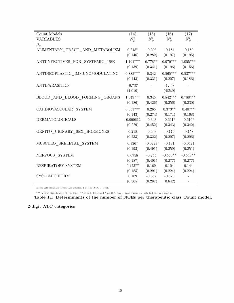
Count Models (14) (15) (16) (17)VARIABLES N t
c′ N tc′ N t
c′ N tc′
βc′ALIMENTARY_TRACT_AND_METABOLISM 0.248* -0.206 -0.184 -0.180
(0.146) (0.282) (0.197) (0.195)
ANTIINFECTIVES_FOR_SYSTEMIC_USE 1.191*** 0.778** 0.970*** 1.055***(0.139) (0.341) (0.196) (0.156)
ANTINEOPLASTIC_IMMUNOMODULATING 0.883*** 0.342 0.565*** 0.537***(0.143) (0.331) (0.207) (0.186)
ANTIPARASITICS -0.737 - -12.68 -(1.010) - (485.9) -
BLOOD_AND_BLOOD_FORMING_ORGANS 1.049*** 0.345 0.842*** 0.788***(0.186) (0.426) (0.256) (0.230)
CARDIOVASCULAR_SYSTEM 0.653*** 0.265 0.373** 0.407**(0.143) (0.274) (0.171) (0.168)
DERMATOLOGICALS -0.000612 -0.343 -0.661* -0.616*(0.229) (0.452) (0.343) (0.342)
GENITO_URINARY_SEX_HORMONES 0.218 -0.403 -0.179 -0.158(0.233) (0.322) (0.297) (0.296)
MUSCULO_SKELETAL_SYSTEM 0.326* -0.0223 -0.131 -0.0421(0.193) (0.491) (0.259) (0.251)
NERVOUS_SYSTEM 0.0758 -0.255 -0.566** -0.548**(0.187) (0.401) (0.277) (0.277)
RESPIRATORY SYSTEM 0.423** 0.169 0.104 0.144(0.185) (0.291) (0.224) (0.224)
SYSTEMIC HORM 0.169 -0.357 -0.579 -(0.365) (0.287) (0.642) -
Note: A ll standard errors are clustered at the ATC-1 level.
*** m eans sign ificance at 1% level, ** at 5 % level and * at 10% level. Year dumm ies included are not shown.
Table 11: Determinants of the number of NCEs per therapeutic class Count model,
2-digit ATC categories
46
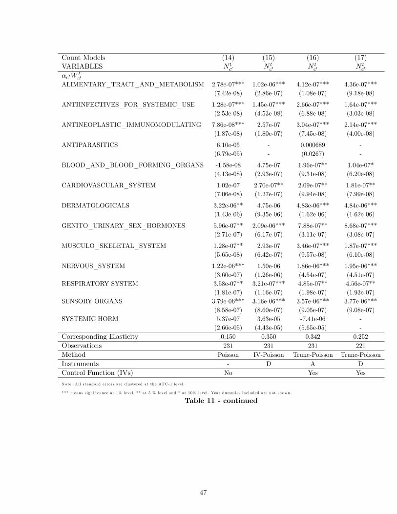
Count Models (14) (15) (16) (17)VARIABLES N t
c′ N tc′ N t
c′ N tc′
αc′Wtc′
ALIMENTARY_TRACT_AND_METABOLISM 2.78e-07*** 1.02e-06*** 4.12e-07*** 4.36e-07***(7.42e-08) (2.86e-07) (1.08e-07) (9.18e-08)
ANTIINFECTIVES_FOR_SYSTEMIC_USE 1.28e-07*** 1.45e-07*** 2.66e-07*** 1.64e-07***(2.53e-08) (4.53e-08) (6.88e-08) (3.03e-08)
ANTINEOPLASTIC_IMMUNOMODULATING 7.86e-08*** 2.57e-07 3.04e-07*** 2.14e-07***(1.87e-08) (1.80e-07) (7.45e-08) (4.00e-08)
ANTIPARASITICS 6.10e-05 - 0.000689 -(6.79e-05) - (0.0267) -
BLOOD_AND_BLOOD_FORMING_ORGANS -1.58e-08 4.75e-07 1.96e-07** 1.04e-07*(4.13e-08) (2.93e-07) (9.31e-08) (6.20e-08)
CARDIOVASCULAR_SYSTEM 1.02e-07 2.70e-07** 2.09e-07** 1.81e-07**(7.06e-08) (1.27e-07) (9.94e-08) (7.99e-08)
DERMATOLOGICALS 3.22e-06** 4.75e-06 4.83e-06*** 4.84e-06***(1.43e-06) (9.35e-06) (1.62e-06) (1.62e-06)
GENITO_URINARY_SEX_HORMONES 5.96e-07** 2.09e-06*** 7.88e-07** 8.68e-07***(2.71e-07) (6.17e-07) (3.11e-07) (3.08e-07)
MUSCULO_SKELETAL_SYSTEM 1.28e-07** 2.93e-07 3.46e-07*** 1.87e-07***(5.65e-08) (6.42e-07) (9.57e-08) (6.10e-08)
NERVOUS_SYSTEM 1.22e-06*** 1.50e-06 1.86e-06*** 1.95e-06***(3.60e-07) (1.26e-06) (4.54e-07) (4.51e-07)
RESPIRATORY SYSTEM 3.58e-07** 3.21e-07*** 4.85e-07** 4.56e-07**(1.81e-07) (1.16e-07) (1.98e-07) (1.93e-07)
SENSORY ORGANS 3.79e-06*** 3.16e-06*** 3.57e-06*** 3.77e-06***(8.58e-07) (8.60e-07) (9.05e-07) (9.08e-07)
SYSTEMIC HORM 5.37e-07 3.63e-05 -7.41e-06 -(2.66e-05) (4.43e-05) (5.65e-05) -
Corresponding Elasticity 0.150 0.350 0.342 0.252Observations 231 231 231 221Method Poisson IV-Poisson Trunc-Poisson Trunc-PoissonInstruments - D A DControl Function (IVs) No Yes Yes
Note: A ll standard errors are clustered at the ATC-1 level.
*** m eans sign ificance at 1% level, ** at 5 % level and * at 10% level. Year dumm ies included are not shown.
Table 11 - continued
47
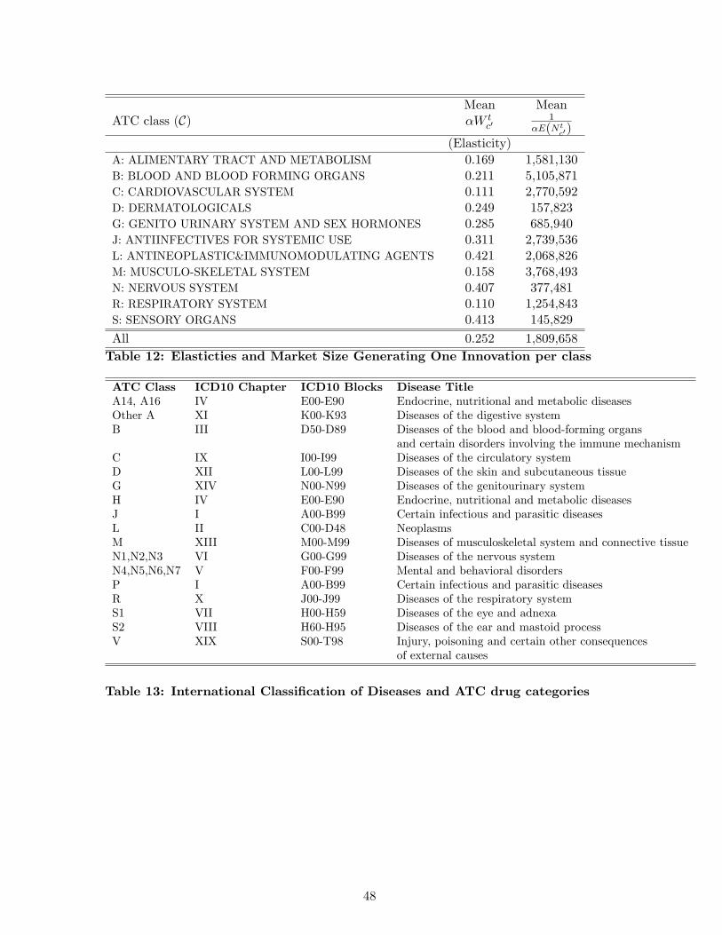
Mean MeanATC class (C) αW t
c′1
αE(Ntc′)
(Elasticity)A: ALIMENTARY TRACT AND METABOLISM 0.169 1,581,130B: BLOOD AND BLOOD FORMING ORGANS 0.211 5,105,871C: CARDIOVASCULAR SYSTEM 0.111 2,770,592D: DERMATOLOGICALS 0.249 157,823G: GENITO URINARY SYSTEM AND SEX HORMONES 0.285 685,940J: ANTIINFECTIVES FOR SYSTEMIC USE 0.311 2,739,536L: ANTINEOPLASTIC&IMMUNOMODULATING AGENTS 0.421 2,068,826M: MUSCULO-SKELETAL SYSTEM 0.158 3,768,493N: NERVOUS SYSTEM 0.407 377,481R: RESPIRATORY SYSTEM 0.110 1,254,843S: SENSORY ORGANS 0.413 145,829
All 0.252 1,809,658Table 12: Elasticties and Market Size Generating One Innovation per class
ATC Class ICD10 Chapter ICD10 Blocks Disease TitleA14, A16 IV E00-E90 Endocrine, nutritional and metabolic diseasesOther A XI K00-K93 Diseases of the digestive systemB III D50-D89 Diseases of the blood and blood-forming organs
and certain disorders involving the immune mechanismC IX I00-I99 Diseases of the circulatory systemD XII L00-L99 Diseases of the skin and subcutaneous tissueG XIV N00-N99 Diseases of the genitourinary systemH IV E00-E90 Endocrine, nutritional and metabolic diseasesJ I A00-B99 Certain infectious and parasitic diseasesL II C00-D48 NeoplasmsM XIII M00-M99 Diseases of musculoskeletal system and connective tissueN1,N2,N3 VI G00-G99 Diseases of the nervous systemN4,N5,N6,N7 V F00-F99 Mental and behavioral disordersP I A00-B99 Certain infectious and parasitic diseasesR X J00-J99 Diseases of the respiratory systemS1 VII H00-H59 Diseases of the eye and adnexaS2 VIII H60-H95 Diseases of the ear and mastoid processV XIX S00-T98 Injury, poisoning and certain other consequences
of external causes
Table 13: International Classification of Diseases and ATC drug categories
48