Embed Size (px)
Citation preview

American Economic Review 2014, 104(2): 495–536 http://dx.doi.org/10.1257/aer.104.2.495
495
Market Size, Competition, and the Product Mix of Exporters†
By Thierry Mayer, Marc J. Melitz, and Gianmarco I. P. Ottaviano*
We build a theoretical model of multi-product firms that highlights how competition across market destinations affects both a firm’s exported product range and product mix. We show how tougher competition in an export market induces a firm to skew its export sales toward its best performing products. We find very strong confirmation of this competitive effect for French exporters across export market destinations. Theoretically, this within-firm change in product mix driven by the trading environment has important repercussions on firm productivity. A calibrated fit to our theoretical model reveals that these productivity effects are potentially quite large. (JEL D21, D24, F13, F14, F41, L11)
Exports by multi-product firms dominate world trade flows. Variations in these trade flows across destinations reflect in part the decisions by multi-product firms to vary the range of their exported products across destinations with different mar-ket conditions.1 In this paper, we further analyze the effects of those export market conditions on the relative export sales of those goods: we refer to this as the firm’s product mix choice. We build a theoretical model of multi-product firms that high-lights how market size and geography (the market sizes of, and bilateral economic distances to, trading partners) affect both a firm’s exported product range and its exported product mix across market destinations. Differences in market sizes and geography generate differences in the toughness of competition across markets. Tougher competition shifts down the entire distribution of markups across products and induces firms to skew their export sales toward their better performing products. We find very strong confirmation of this competitive effect for French exporters
1 See Mayer and Ottaviano (2008) for Europe, Bernard et al. (2007) for the United States, and Arkolakis and Muendler (2010) for Brazil.
* Mayer: Sciences-Po, 28 rue des Saints-Pères, 75007 Paris, France, CEPII, and CEPR (e-mail: [email protected]); Melitz: Department of Economics, Harvard University, Cambridge, MA 02138, CEPR, and NBER (e-mail: [email protected]); Ottaviano: London School of Economics, Houghton Street, London WC2A 2AE, United Kingdom, CEP, and CEPR (e-mail: [email protected]). This paper is produced as part of the project “European firms in a global economy: Internal policies for external competitiveness” (EFIGE), a collaborative project funded by the European Commission’s Seventh Research Framework Programme, Contract #225551. The views expressed in this publication are the sole responsibility of the authors and do not necessarily reflect the views of the European Commission. We thank the French customs administration and CNIS for making the exports data available at CEPII. We thank two anonymous referees, Philippe Martin, Giordano Mion, Peter Neary, Steve Redding, and Dan Trefler for helpful comments and suggestions. We are also grateful to seminar participants for all the useful feedback we received. Ottaviano thanks Bocconi University, CEP, MIUR, and the European Commission for financial support. Melitz thanks the Sloan Foundation for financial support. Melitz and Ottaviano thank Sciences Po and CEPII for their hospitality while part of this paper was written.
† Go to http://dx.doi.org/10.1257/aer.104.2.495 to visit the article page for additional materials and author disclosure statement(s).

496 THE AMERICAN ECONOMIC REVIEW FEBRUARY 2014
across export market destinations. Our theoretical model shows how this effect of export market competition on a firm’s product mix then translates into differences in measured firm productivity: when a firm skews its production toward better per-forming products, it also allocates relatively more workers to the production of those goods and raises its overall output (and sales) per worker. Thus, a firm producing a given set of products with given unit input requirements will produce relatively more output and sales per worker (across products) when it exports to markets with tougher competition. To our knowledge, this is a new channel through which com-petition (both in export markets and at home) affects firm-level productivity. This effect of competition on firm-level productivity is compounded by another channel that operates through the endogenous response of the firm’s product range: firms respond to increased competition by dropping their worst performing products.2
Feenstra and Ma (2008) and Eckel and Neary (2010) also build theoretical mod-els of multi-product firms that highlight the effect of competition on the distribution of firm product sales. Both models incorporate the cannibalization effect that occurs as large firms expand their product range. In our model, we rely on the competition effects from the demand side, which are driven by variations in the number of sellers and their average prices across export markets. The cannibalization effect does not occur as a continuum of firms each produce a discrete number of products and thus never attain finite mass. The benefits of this simplification is that we can consider an open economy equilibrium with multiple asymmetric countries and asymmetric trade barriers whereas Feenstra and Ma (2008) and Eckel and Neary (2010) restrict their analysis to a single globalized world with no trade barriers. Thus, our model is able to capture the key role of geography in shaping differences in competition across export market destinations.3
Another approach to the modeling of multi-product firms relies on a nested CES structure for preferences, where a continuum of firms produce a continuum of prod-ucts. The cannibalization effect is ruled out by restricting the nests in which firms can introduce new products. Allanson and Montagna (2005) consider such a model in a closed economy, while Arkolakis and Muendler (2010) and Bernard, Redding, and Schott (2011) develop extensions to open economies. Given the CES structure of preferences and the continuum assumptions, markups across all firms and prod-ucts are exogenously fixed. Thus, differences in market conditions or proportional reductions in trade costs have no effect on a firm’s product mix choice (the rela-tive distribution of export sales across products). In contrast, variations in markups across destinations (driven by differences in competition) generate differences in relative exports across destinations in our model: a given firm selling the same two products across different markets will export relatively more of the better perform-ing product in markets where competition is tougher. In our comprehensive data
2 Bernard, Redding, and Schott (2011) and Eckel and Neary (2010) emphasize this second channel. They show how trade liberalization between symmetric countries induces firms to drop their worst performing products (a focus on core competencies) leading to intra-firm productivity gains. We discuss those papers in further detail below.
3 Nocke and Yeaple (2006) and Baldwin and Gu (2009) also develop models with multi-product firms and a pro-competitive effect coming from the demand side. These models investigate the effects of globalization on a firm’s product scope and average production levels per product. However, those models consider the case of firms producing symmetric products whereas we focus on the effects of competition on the within-firm distribution of product sales.

497MAYER ET AL.: MARKET SIZE, COMPETITION, AND PRODUCT MIXVOL. 104 NO. 2
covering nearly all French exports, we find that there is substantial variation in this relative export ratio across French export destinations, and that this variation is con-sistently related to differences in market size and geography across those destina-tions (market size and geography both affect the toughness of competition across destinations). French exporters substantially skew their export sales toward their better performing products in markets where they face tougher competition.
Theoretically, we show how this effect of tougher competition in an export market on the exported product mix is also associated with an increase in productivity for the set of exported products to that market. We show how firm-level measures of exported output per worker as well as deflated sales per worker for a given export destination (counting only the exported units to a given destination and the associ-ated labor used to produce those units) increase with tougher competition in that destination. This effect of competition on firm productivity holds even when one fixes the set of products exported, thus eliminating any potential effects from the extensive (product) margin of trade. Then, the firm-level productivity increase is entirely driven by the response of the firm’s product mix: producing relatively more of the better performing products raises measured firm productivity. We use our theoretical model to calibrate the relationship between the skewness of the French exporters’ product mix and a productivity average for those exporters. We find that our measured variation in product mix skewness across destinations corresponds to large differences in productivity. The effect of a doubling of destination country GDP on the French exporters’ product mix corresponds to a measured productivity differential between 4 percent and 7 percent.
Our model also features a response of the extensive margin of trade: tougher competition in the domestic market induces firms to reduce the set of produced products, and tougher competition in an export market induces exporters to reduce the set of exported products. We do not emphasize these results for the extensive margin because they are quite sensitive to the specification of fixed production and export costs. In order to maintain the tractability of our multi-country asymmetric open economy, we abstract from those fixed costs (increasing returns are generated uniquely from the fixed/sunk entry cost). Conditional on the production and export of given sets of products, such fixed costs would not affect the relative production or export levels of those products. These are the product mix outcomes that we empha-size (and for which we find strong empirical support).
Although we focus our empirical analysis on these novel cross-sectional predic-tions, our model also predicts extensive and intensive margin responses over time to multilateral trade liberalization. Such liberalization induces an increase in the tough-ness of competition in each country. In response, firms reduce the number of prod-ucts they produce and skew production and sales (in each destination) toward their better performing products. These firm-level responses have all been documented in recent empirical work on the effects of trade liberalization in North America. Baldwin and Gu (2009); Bernard, Redding, and Schott (2011), and Iacovone and Javorcik (2008) all report that (respectively) Canadian, US, and Mexican firms have reduced the number of products they produce during these trade-liberalization epi-sodes. Baldwin and Gu (2009) and Bernard, Redding, and Schott (2011) further report that the Canada-United States Free Trade Agreement (CUSFTA) induced a significant increase in the skewness of production across products (an increase

498 THE AMERICAN ECONOMIC REVIEW FEBRUARY 2014
in entropy). Iacovone and Javorcik (2008) separately measure the skewness of Mexican firms’ export sales to the United States. They report an increase in this skewness following NAFTA: they show that Mexican firms expanded their exports of their better performing products (higher market shares) significantly more than those for their worse performing exported products during the period of trade expan-sion from 1994 –2003.
Our paper proceeds as follows. We first develop a closed economy version of our model in order to focus on the endogenous responses of a firm’s product scope and product mix to market conditions. We highlight how competition affects the skew-ness of a firm’s product mix, and how this translates into differences in firm produc-tivity. Thus, even in a closed economy, increases in market size lead to increases in within-firm productivity via this product mix response. We then develop the open economy version of our model with multiple asymmetric countries and an arbitrary matrix of bilateral trade costs. The equilibrium connects differences in market size and geography to the toughness of competition in every market, and how the latter shapes a firm’s exported product mix to that destination. We then move on to our empirical test for this exported product mix response for French firms. We show how destination market size as well as its geography induce increased skewness in the firms’ exported product mix to that destination. In the last section before concluding we quantify the economic significance of those measured differences in export skewness for productivity.
I. Closed Economy
Our model is based on an extension of Melitz and Ottaviano (2008) that allows firms to endogenously determine the set of products that they produce. We start with a closed economy version of this model where L consumers each supply one unit of labor.
A. Preferences and Demand
Preferences are defined over a continuum of differentiated varieties indexed by i ∈ Ω, and a homogenous good chosen as numeraire. All consumers share the same utility function given by
(1) U = q 0 c + α ∫
i∈Ω
q i c di − 1 _
2 γ ∫
i∈Ω
( q i c ) 2 di − 1 _
2 η ( ∫
i∈Ω
q i c di )
2 ,
where q 0 c and q i c represent the individual consumption levels of the numeraire good
and each variety i. The demand parameters α, η, and γ are all positive. The param-eters α and η index the substitution pattern between the differentiated varieties and the numeraire: increases in α and decreases in η both shift out the demand for the differentiated varieties relative to the numeraire. The parameter γ indexes the degree of product differentiation between the varieties. In the limit when γ = 0, consum-ers only care about their consumption level over all varieties, Q c = ∫ i∈Ω
q i c di, and the varieties are then perfect substitutes. The degree of product differentiation increases with γ as consumers give increasing weight to smoothing consumption levels across varieties.

499MAYER ET AL.: MARKET SIZE, COMPETITION, AND PRODUCT MIXVOL. 104 NO. 2
Our specification of preferences intentionally does not distinguish between the varieties produced by the same firm relative to varieties produced by other firms. We do not see any clear reason to enforce that varieties produced by a firm be closer sub-stitutes than varieties produced by different firms—or vice-versa. Of course, some firms operate across sectors, in which case the varieties produced in different sec-tors would be more differentiated than varieties produced by other firms within the same sector. We eliminate those cross-sector, within-firm, varieties in our empirical work by restricting our analysis to the range of varieties produced by a firm within a sector classification.
The marginal utilities for all varieties are bounded, and a consumer may not have positive demand for any particular variety. We assume that consumers have positive demand for the numeraire good ( q 0 c
> 0). The inverse demand for each variety i is then given by
(2) p i = α − γ q i c − η Q c ,
whenever q i c > 0. Let Ω ∗ ⊂ Ω be the subset of varieties that are consumed (such that q i c > 0 ). Equation (2) can then be inverted to yield the linear market demand system for these varieties:
(3) q i ≡ L q i c = αL _ η M + γ − L _ γ p i + η M _ η M + γ L _ γ _ p , ∀i ∈ Ω ∗ ,
where M is the measure of consumed varieties in Ω ∗ and _ p = ( 1/M ) ∫
i∈ Ω ∗ p i di is
their average price. The set Ω ∗ is the largest subset of Ω that satisfies
(4) p i ≤ 1 _ η M + γ ( γ α + η M _ p ) ≡ p max ,
where the right-hand-side price bound p max represents the price at which demand for a variety is driven to zero. Note that (2) implies p max ≤ α. In contrast to the case of CES demand, the price elasticity of demand, ε i ≡ | ( ∂ q i /∂ p i ) ( p i / q i ) | = [ ( p max / p i ) − 1 ] −1 , is not uniquely determined by the level of product differen-tiation γ. Given the latter, lower average prices
_ p or a larger number of competing
varieties M induce a decrease in the price bound p max and an increase in the price elasticity of demand ε i at any given p i . We characterize this as a “tougher” competi-tive environment.4
Welfare can be evaluated using the indirect utility function associated with (1):
(5) U = I c + 1 _ 2 ( η +
γ _
M )
−1 ( α − _ p ) 2 + 1 _
2 M _ γ σ p 2 ,
where I c is the consumer’s income and σ p 2 = ( 1/M ) ∫ i∈ Ω ∗ ( p i − _ p ) 2 di repre-
sents the variance of prices. To ensure positive demand levels for the numeraire,
4 We also note that, given this competitive environment (given N and _ p ), the price elasticity ε i monotonically
increases with the price p i along the demand curve.
500 THE AMERICAN ECONOMIC REVIEW FEBRUARY 2014
we assume that I c > ∫ i∈ Ω ∗ p i q i c di = _ p Q c − M σ p 2 /γ. Welfare naturally rises with
decreases in average prices _ p . It also rises with increases in the variance of prices
σ p 2 (holding the mean price _ p constant), as consumers then re-optimize their
purchases by shifting expenditures toward lower priced varieties as well as the numeraire good.5 Finally, the demand system exhibits “love of variety”: holding the distribution of prices constant (namely holding the mean
_ p and variance σ p 2 of prices
constant), welfare rises with increases in product variety M.
B. Production and Firm Behavior
Labor is the only factor of production and is inelastically supplied in a competitive market. The numeraire good is produced under constant returns to scale at unit cost; its market is also competitive. These assumptions imply a unit wage. Entry in the differentiated product sector is costly as each firm incurs product development and production startup costs. Subsequent production of each variety exhibits constant returns to scale. While it may decide to produce more than one variety, each firm has one key variety corresponding to its “core competency.” This is associated with a core marginal cost c (equal to unit labor requirement).6 Research and development yield uncertain outcomes for c, and firms learn about this cost level only after mak-ing the irreversible investment f E required for entry. We model this as a draw from a common (and known) distribution G(c) with support on [0, c M ].
A firm can introduce any number of new varieties, but each additional variety entails an additional customization cost as it pulls a firm away from its core com-petency. This entails incrementally higher marginal costs of production for those varieties. The divergence from a firm’s core competency may also be reflected in diminished product quality/appeal. For simplicity, we maintain product symmetry on the demand side and capture any decrease in product appeal as an increased pro-duction cost. We refer to this incremental production cost as a customization cost.
We index by m the varieties produced by the same firm in increasing order of dis-tance from their core competency m = 0 (the firm’s core variety). We then denote v(m, c) the marginal cost for variety m produced by a firm with core marginal cost c and assume v(m, c) = ω −m c with ω ∈ (0, 1). This defines a firm-level “competence ladder” with geometrically increasing customization costs. This modeling approach is isomorphic to one where we label the product ladder as reflecting decreasing quality/product appeal and insert the geometric term as a preference parameter mul-tiplying quantities in the utility function (1). Our modeling approach also nests the case of single-product firms as the geometric step size becomes arbitrarily large (ω goes to zero); firms will then only be able to produce their core variety.
Since the entry cost is sunk, firms that can cover the marginal cost of their core variety survive and produce. All other firms exit the industry. Surviving firms maximize their profits using the residual demand function (3). In so doing, those firms take the average price level
_ p and total number of varieties M as given.
5 This welfare measure reflects the reduced consumption of the numeraire to account for the labor resources used to cover the entry costs.
6 We use the same concept of a firm’s core competency as Eckel and Neary (2010). For simplicity, we do not model any fixed production costs. This would significantly increase the complexity of our model without yielding much new insight.
501MAYER ET AL.: MARKET SIZE, COMPETITION, AND PRODUCT MIXVOL. 104 NO. 2
This monopolistic competition outcome is maintained with multi-product firms as any firm can only produce a countable number of products, which is a subset of measure zero of the total mass of varieties M.
The profit maximizing price p(v) and output level q(v) of a variety with cost v must then satisfy
(6) q(v) = L _ γ [ p(v) − v ] .
The profit maximizing price p(v) may be above the price bound p max from (4), in which case the variety is not supplied. Let v D reference the cutoff cost for a variety to be profitably produced. This variety earns zero profit as its price is driven down to its marginal cost, p( v D ) = v D = p max , and its demand level q( v D ) is driven to zero. Let r(v) = p(v)q(v), π(v) = r(v) − q(v)v, λ(v) = p(v) − v denote the revenue, profit, and (absolute) markup of a variety with cost v. All these performance measures can then be written as functions of v and v D only:7
(7) p(v) = 1 _ 2 ( v D + v ) ,
λ(v) = 1 _ 2 ( v D − v ) ,
q(v) = L _ 2γ
( v D − v ) ,
r(v) = L _ 4 γ
[ ( v D ) 2 − v 2 ] ,
π(v) = L _ 4 γ
( v D − v ) 2 .
The threshold cost v D thus summarizes the competitive environment for the perfor-mance measures of all produced varieties. As expected, lower cost varieties have lower prices and earn higher revenues and profits than varieties with higher costs. However, lower cost varieties do not pass on all of the cost differential to consum-ers in the form of lower prices: they also have higher markups (in both absolute and relative terms) than varieties with higher costs.8
Firms with core competency v > v D cannot profitably produce their core vari-ety and exit. Hence, c D = v D is also the cutoff for firm survival and measures the “toughness” of competition in the market: it is a sufficient statistic for all
7 Given the absence of cannibalization motive, these variety level performance measures are identical to the single product case studied in Melitz and Ottaviano (2008). This tractability allows us to analytically solve the closed and open equilibria with heterogenous firms (and asymmetric countries in the open economy).
8 De Loecker et al. (2012) find empirical support for these properties, both across and within firms, in the case of Indian multi-product firms.
502 THE AMERICAN ECONOMIC REVIEW FEBRUARY 2014
performance measures across varieties and firms.9 We assume that c M is high enough that it is always above c D , so exit rates are always positive. All firms with core cost c < c D earn positive profits (gross of the entry cost) on their core variet-ies and remain in the industry. Some firms will also earn positive profits from the introduction of additional varieties. In particular, firms with cost c such that v(m, c) ≤ v D ⇔ c ≤ ω m c D earn positive profits on their m th additional variety and thus produce at least m + 1 varieties. The total number of varieties produced by a firm with cost c is
(8) M(c) = { 0
max { m | c ≤ ω m c D } + 1
if c > c D ,
if c ≤ c D ,
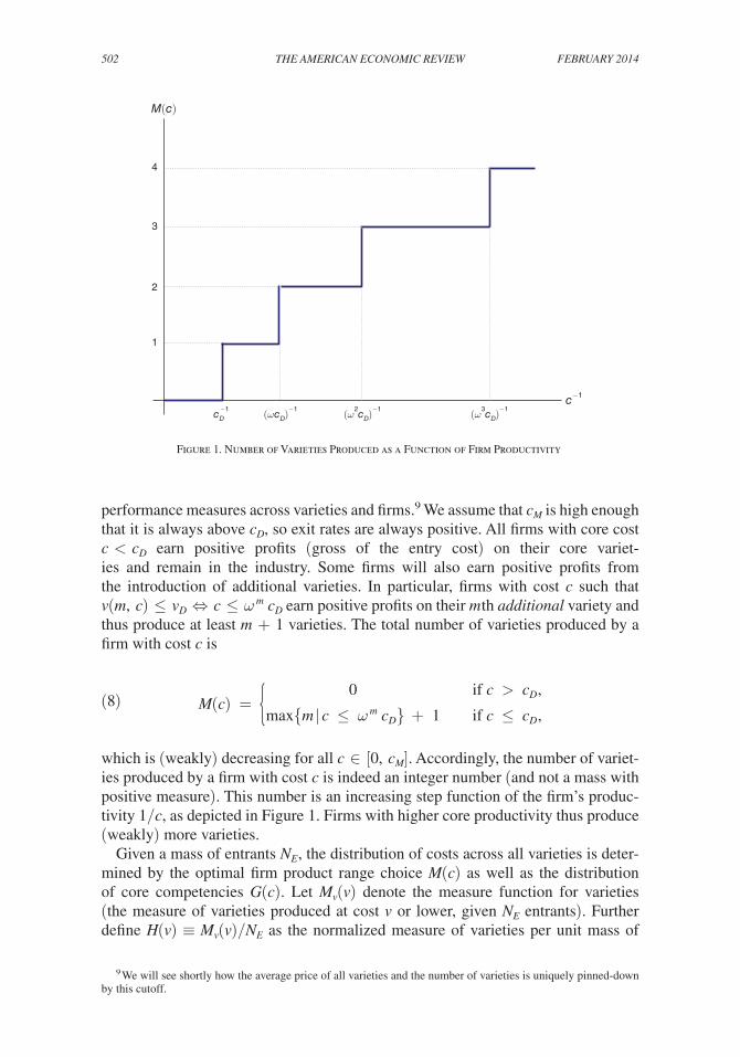
which is (weakly) decreasing for all c ∈ [0, c M ]. Accordingly, the number of variet-ies produced by a firm with cost c is indeed an integer number (and not a mass with positive measure). This number is an increasing step function of the firm’s produc-tivity 1/c, as depicted in Figure 1. Firms with higher core productivity thus produce (weakly) more varieties.
Given a mass of entrants N E , the distribution of costs across all varieties is deter-mined by the optimal firm product range choice M(c) as well as the distribution of core competencies G(c). Let M v (v) denote the measure function for varieties (the measure of varieties produced at cost v or lower, given N E entrants). Further define H(v) ≡ M v (v)/ N E as the normalized measure of varieties per unit mass of
9 We will see shortly how the average price of all varieties and the number of varieties is uniquely pinned-down by this cutoff.
Figure 1. Number of Varieties Produced as a Function of Firm Productivity
M(c)
4
3
2
1
c−1
cD−1 (ωcD)
−1 (ω2cD)
−1 (ω3cD)
−1

503MAYER ET AL.: MARKET SIZE, COMPETITION, AND PRODUCT MIXVOL. 104 NO. 2
entrants. Then H(v) = ∑ m=0 ∞ G( ω m v) and is exogenously determined from G(·)
and ω. Given a unit mass of entrants, there will be a mass G(v) of varieties with cost v or less; a mass G(ωv) of first additional varieties (with cost v or less); a mass G( ω 2 v) of second additional varieties; and so forth. The measure H(v) sums over all these varieties.
C. Free Entry and Equilibrium
Prior to entry, the expected firm profit is ∫ 0 c D Π(c) dG(c) − f E where
(9) Π(c) ≡ ∑ m=0
M(c)−1
π ( v ( m, c ) )
denotes the profit of a firm with cost c. If this profit were negative for all c s, no firms would enter the industry. As long as some firms produce, the expected profit is driven to zero by the unrestricted entry of new firms. This yields the equilibrium free entry condition:
(10) ∫ 0 c D
Π(c) dG(c) = ∫ 0 c D
[ ∑ { m | ω −m c≤ c D }
π ( ω −m c ) ] dG(c)
= ∑ m=0
∞
[ ∫ 0 ω m c D
π ( ω −m c ) dG(c) ] = f E ,
where the second equality first averages over the m th produced variety by all firms, then sums over m.
The free entry condition (10) determines the cost cutoff c D = v D . This cutoff, in turn, determines the aggregate mass of varieties, since v D = p( v D ) must also be equal to the zero demand price threshold in (4):
v D = 1 _ η M + γ ( γ α + η M _ p ) .
The aggregate mass of varieties is then
M = 2γ _ η α − v D
_ v D − _ v ,
where the average cost of all varieties,
_ v = 1 _
M ∫
0 v D
vd M v (v) = 1 _ N E H( v D )
∫ 0 v D
v N E dH(v) = 1 _ H( v D )
∫ 0 v D
v dH(v),

504 THE AMERICAN ECONOMIC REVIEW FEBRUARY 2014
depends only on v D .10 Similarly, this cutoff also uniquely pins down the average price across all varieties:
_ p = 1 _
M ∫
0 v D
p(v) d M v (v) = 1 _ H( v D )
∫ 0 v D
p(v) dH(v).
Finally, the mass of entrants is given by N E = M/H( v D ), which can in turn be used to obtain the mass of producing firms N = N E G( c D ).
D. Parametrization of Technology
All the results derived so far hold for any distribution of core cost draws G(c). However, in order to simplify some of the ensuing analysis, we use a specific param-etrization for this distribution. In particular, we assume that core productivity draws 1/c follow a Pareto distribution with lower productivity bound 1/ c M and shape parameter k ≥ 1. This implies a distribution of cost draws c given by
(11) G(c) = ( c _ c M ) k , c ∈ [0, c M ].
The shape parameter k indexes the dispersion of cost draws. When k = 1, the cost distribution is uniform on [0, c M ]. As k increases, the relative number of high cost firms increases, and the cost distribution is more concentrated at these higher cost levels. As k goes to infinity, the distribution becomes degenerate at c M . Any trunca-tion of the cost distribution from above will retain the same distribution function and shape parameter k. The productivity distribution of surviving firms will therefore also be Pareto with shape k, and the truncated cost distribution will be given by G D (c) = ( c/ c D ) k , c ∈ [0, c D ].
When core competencies are distributed Pareto, then all produced varieties will share the same Pareto distribution:
(12) H(c) = ∑ m=0
∞
G( ω m c) = ΩG(c),
where Ω = ( 1 − ω k ) −1 > 1 is an index of multi-product flexibility (which varies monotonically with ω). In equilibrium, this index will also be equal to the average number of products produced across all surviving firms:
M _ N
= H( v D ) N E
_ G( c D ) N E
= Ω.
10 We also use the relationship between average cost and price _ v = 2
_ p − v D , which is obtained from (7).
505MAYER ET AL.: MARKET SIZE, COMPETITION, AND PRODUCT MIXVOL. 104 NO. 2
The Pareto parametrization also yields a simple closed-form solution for the cost cutoff c D from the free entry condition (10):
(13) c D = [ γϕ _
LΩ ] 1 _
k+2
,
where ϕ ≡ 2(k + 1)(k + 2) ( c M ) k f E is a technology index that combines the effects of better distribution of cost draws (lower c M ) and lower entry costs f E . We assume that c M > √
____________________ [ 2(k + 1)(k + 2)γ f E ] / ( L Ω ) in order to ensure c D < c M as was previ-
ously anticipated. We also note that, as the customization cost for non-core varieties becomes infinitely large (ω → 0), multi-product flexibility Ω goes to 1, and (13) then boils down to the single-product case studied by Melitz and Ottaviano (2008).
E. Equilibrium with Multi-Product Firms
Equation (13) summarizes how technology (referenced by the distribution of cost draws and the sunk entry cost), market size, product differentiation, and multi-product flexibility affect the toughness of competition in the market equilibrium. Increases in market size, technology improvements (a fall in c M or f E ), and increases in product substitutability (a rise in γ) all lead to tougher competition in the market and thus to an equilibrium with a lower cost cutoff c D . As multi-product flexibility Ω increases, firms respond by introducing more products. This additional production is skewed toward the better performing firms and also leads to tougher competition and a lower c D cutoff.
A market with tougher competition (lower c D ) also features more product vari-ety M and a lower average price
_ p (due to the combined effect of product selec-
tion toward lower cost varieties and of lower markups). Both of these contribute to higher welfare U. Given our Pareto parametrization, we can write all of these variables as simple closed form functions of the cost cutoff c D :
(14) M = 2(k + 1)γ _ η α − c D
_ c D ,
_ p = 2k + 1
_ 2k + 2
c D ,
U = 1 + 1 _ 2η
( α − c D ) ( α − k + 1 _
k + 2 c D ) .
Increases in the toughness of competition do not affect the average number of vari-eties produced per firm M/N = Ω because the mass of surviving firms N rises by the same proportion as the mass of produced varieties M.11 However, each firm
11 This exact offsetting effect between the number of firms and the number of products is driven by our functional form assumptions. However, the downward shift in M(c) in response to competition (described next) holds for a much more general set of parameterizations.
506 THE AMERICAN ECONOMIC REVIEW FEBRUARY 2014
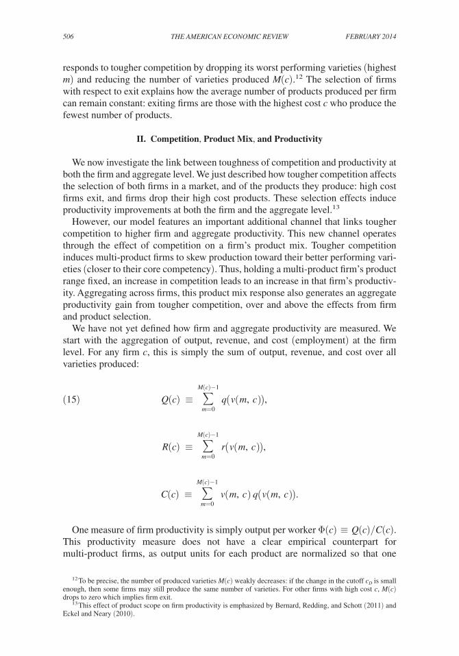
responds to tougher competition by dropping its worst performing varieties (highest m) and reducing the number of varieties produced M(c).12 The selection of firms with respect to exit explains how the average number of products produced per firm can remain constant: exiting firms are those with the highest cost c who produce the fewest number of products.
II. Competition, Product Mix, and Productivity
We now investigate the link between toughness of competition and productivity at both the firm and aggregate level. We just described how tougher competition affects the selection of both firms in a market, and of the products they produce: high cost firms exit, and firms drop their high cost products. These selection effects induce productivity improvements at both the firm and the aggregate level.13
However, our model features an important additional channel that links tougher competition to higher firm and aggregate productivity. This new channel operates through the effect of competition on a firm’s product mix. Tougher competition induces multi-product firms to skew production toward their better performing vari-eties (closer to their core competency). Thus, holding a multi-product firm’s product range fixed, an increase in competition leads to an increase in that firm’s productiv-ity. Aggregating across firms, this product mix response also generates an aggregate productivity gain from tougher competition, over and above the effects from firm and product selection.
We have not yet defined how firm and aggregate productivity are measured. We start with the aggregation of output, revenue, and cost (employment) at the firm level. For any firm c, this is simply the sum of output, revenue, and cost over all varieties produced:
(15) Q(c) ≡ ∑ m=0
M(c)−1
q ( v ( m, c ) ) ,
R(c) ≡ ∑ m=0
M(c)−1
r ( v ( m, c ) ) ,
C(c) ≡ ∑ m=0
M(c)−1
v ( m, c ) q ( v ( m, c ) ) .
One measure of firm productivity is simply output per worker Φ(c) ≡ Q(c)/C(c). This productivity measure does not have a clear empirical counterpart for multi-product firms, as output units for each product are normalized so that one
12 To be precise, the number of produced varieties M(c) weakly decreases: if the change in the cutoff c D is small enough, then some firms may still produce the same number of varieties. For other firms with high cost c, M(c) drops to zero which implies firm exit.
13 This effect of product scope on firm productivity is emphasized by Bernard, Redding, and Schott (2011) and Eckel and Neary (2010).

507MAYER ET AL.: MARKET SIZE, COMPETITION, AND PRODUCT MIXVOL. 104 NO. 2
unit of each product generates the same utility for the consumer (this is the implicit normalization behind the product symmetry in the utility function). A firm’s deflated sales per worker Φ R (c) ≡ [ R(c)/
_ P ] /C(c) provides another productivity measure
that has a clear empirical counterpart. For this productivity measure, we need to define the price deflator
_ P . We choose
_ P ≡
∫ 0 c D
R(c) dG(c) __
∫ 0 c D
Q(c) dG(c) = k + 1
_ k + 2
c D .
This is the average of all the variety prices p(v) weighted by their output share. We could also have used the unweighted price average
_ p that we previously defined, or
an average weighted by a variety’s revenue share (i.e., its market share) instead of output share. In our model, all of these price averages only differ by a multiplicative constant, so the effects of competition (changes in the cutoff c D ) on productivity will not depend on this choice of price averages.14 We define the aggregate counterparts to our two firm productivity measures as industry output per worker and industry deflated sales per worker:
_ Φ ≡
∫ 0 c D
Q(c) dG(c) __
∫ 0 c D
C(c) dG(c) ,
_ Φ R =
[ ∫ 0 c D
R(c) dG(c) ] / _ P __
∫ 0 c D
C(c) dG(c) .
Our choice of the price deflator _ P then implies that these two aggregate productivity
measures coincide:15
(16) _ Φ =
_ Φ R = k + 2
_ k 1 _ c D .
Equation (16) summarizes the overall effect of tougher competition on aggregate productivity gains. This aggregate response of productivity combines the effects of competition on both firm productivity and inter-firm reallocations (including entry and exit). We now detail how tougher competition induces improvements in firm productivity through its impact on a firm’s product mix. In Appendix B, we show that both firm productivity measures, Φ(c) and Φ R (c), increase for all multi-product firms when competition increases ( c D decreases). The key component of this proof is that, holding a firm’s product scope constant (a given number M > 1 of non-core varieties produced), firm productivity over that product scope (output or deflated sales of those M products per worker producing those products) increases whenever competition increases. This effect of competition on firm productivity, by construc-tion, is entirely driven by the response of the firm’s product mix.
14 As we previously reported in equation (14), the unweighted price average is _ p = [ ( 2k + 1 ) / ( 2k + 2 ) ] c D ; and
the average weighted by market share is [(6k + 2 k 2 + 3)/(2 k 2 + 8k + 6)] c D .15 If we had picked one of the other price averages, the two aggregate productivity measures would differ by a
multiplicative constant.

508 THE AMERICAN ECONOMIC REVIEW FEBRUARY 2014
To isolate this product mix response to competition, consider two varieties m and m′ produced by a firm with cost c. Assume that m < m′ so that variety m is closer to the core. The ratio of the firm’s output of the two varieties is given by
q(v ( m, c ) ) _
q(v ( m′ , c ) ) =
c D − ω −m c _
c D − ω − m′ c .
As competition increases ( c D decreases), this ratio increases, implying that the firm skews its production toward its core varieties. This happens because the increased competition increases the price elasticity of demand for all products. At a con-stant relative price p(v(m, c))/p(v( m′ , c)), the higher price elasticity translates into higher relative demand q(v(m, c))/q(v( m′ , c)) and sales r (v(m, c))/r(v( m′ , c)) for good m (relative to m′ ).16 In our specific demand parametrization, there is a further increase in relative demand and sales, because markups drop more for good m than m′ , which implies that the relative price p(v(m, c))/p(v( m′ , c)) decreases.17 It is this reallocation of output toward better performing products (also mirrored by a real-location of production labor toward those products) that generates the productivity increases within the firm. In other words, tougher competition skews the distribution of employment, output, and sales toward the better performing varieties (closer to the core), while it flattens the firm’s distribution of prices.
In the open economy version of our model that we develop in the next section, we show how firms respond to tougher competition in export markets in very similar ways by skewing their exported product mix toward their better performing prod-ucts. Our empirical results confirm a strong effect of such a link between competi-tion and product mix.
III. Open Economy
We now turn to the open economy in order to examine how market size and geog-raphy determine differences in the toughness of competition across markets—and how the latter translates into differences in the exporters’ product mix. We allow for an arbitrary number of countries and asymmetric trade costs. Let J denote the num-ber of countries, indexed by l = 1, … , J. The markets are segmented, although any produced variety can be exported from country l to country h subject to an iceberg trade cost τ lh > 1. Thus, the delivered cost for variety m exported to country h by a firm with core competency c in country l is τ lh v(m, c) = τ lh ω −m c.
A. Equilibrium with Asymmetric Countries
Let p l max denote the price threshold for positive demand in market l. Then (4) implies
(17) p l max = 1 _ η M l + γ ( γ α + η M l _ p l ) ,
16 For the result on relative sales, we are assuming that the price elasticity of demand (ε) is larger than one.17 Good m closer to the core initially has a higher markup than good m′ ; see (7).

509MAYER ET AL.: MARKET SIZE, COMPETITION, AND PRODUCT MIXVOL. 104 NO. 2
where M l is the total number of products selling in country l (the total number of domestic and exported varieties) and
_ p l is their average price. Let π ll (v) and π lh (v)
represent the maximized value of profits from domestic and export sales to country h for a variety with cost v produced in country l. (We use the subscript ll to denote domestic variables, pertaining to firms located in l.) The cost cutoffs for profitable domestic production and for profitable exports must satisfy
(18) v ll = sup { c : π ll (v) > 0 } = p l max ,
v lh = sup { c : π lh (v) > 0 } = p h max _ τ lh ,
and thus v lh = v hh / τ lh . As was the case in the closed economy, the cutoff v ll , l = 1, … , J, summarizes all the effects of market conditions in country l relevant for all firm performance measures. The profit functions can then be written as a function of these cutoffs (assuming that markets are segmented, as in Melitz and Ottaviano, 2008):
(19) π ll (v) = L l _ 4 γ
( v ll − v ) 2 ,
π lh (v) = L h _ 4γ
τ lh 2 ( v lh − v ) 2 =
L h _ 4γ
( v hh − τ lh v ) 2 .
As in the closed economy, c ll = v ll will be the cutoff for firm survival in country l (cutoff for domestic sales of firms producing in l ). Similarly, c lh = v lh will be the firm export cutoff from l to h (no firm with c > c lh can profitably export any varieties from l to h). A firm with core competency c will produce all varieties m such that π ll ( v(m, c) ) ≥ 0 ; it will export to h the subset of varieties m such that π lh ( v(m, c) ) ≥ 0. The total number of varieties produced and exported to h by a firm with cost c in country l are thus
M ll (c) = { 0
max { m | c ≤ ω m c ll } + 1
if c > c ll , if c ≤ c ll ,
M lh (c) = { 0
max { m | c ≤ ω m c lh } + 1
if c > c lh , if c ≤ c lh .
We can then define a firm’s total domestic and export profits by aggregating over these varieties:
Π ll (c) = ∑ m=0
M ll (c)−1
π ll ( v ( m, c ) ) , Π lh (c) = ∑ m=0
M lh (c)−1
π lh ( v ( m, c ) ) .

510 THE AMERICAN ECONOMIC REVIEW FEBRUARY 2014
Entry is unrestricted in all countries. Firms choose a production location prior to entry and paying the sunk entry cost. We assume that the entry cost f E and cost distribution G(c) are common across countries (although this can be relaxed).18 We maintain our Pareto parametrization (11) for this distribution. A prospective entrant’s expected profits will then be given by
∫ 0 c ll
Π ll (c) dG(c) + ∑ h≠l
∫ 0 c lh
Π lh (c) dG(c)
= ∑ m=0
∞
[ ∫ 0 ω m c ll
π ll ( ω −m c ) dG(c) ] + ∑ h≠l
∑ m=0
∞
[ ∫ 0 ω m c lh
π lh ( ω −m c ) dG(c) ]
= 1 __ 2γ (k + 1)(k + 2) c M k
[ L l Ω c ll k+2 + ∑
h≠l
L h Ω τ lh 2 c lh k+2 ]
= Ω __ 2γ (k + 1)(k + 2) c M k
[ L l c ll k+2 + ∑
h≠l
L h τ lh −k c hh k+2 ] .
Setting the expected profit equal to the entry cost yields the free entry conditions:
(20) ∑ h=1
J
ρ lh L h c hh k+2 = γϕ _
Ω l = 1, … , J,
where ρ lh ≡ τ lh −k < 1 is a measure of “freeness” of trade from country l to country h that varies inversely with the trade costs τ lh . The technology index ϕ is the same as in the closed economy case.
The free entry conditions (20) yield a system of J equations that can be solved for the J equilibrium domestic cutoffs using Cramer’s rule:
(21) c hh = ( γϕ _
Ω ∑ l=1
J
| C lh | _
| P | 1 _ L h
)
1 _ k+2
,
18 Differences in the support for this distribution could also be introduced as in Melitz and Ottaviano (2008).

511MAYER ET AL.: MARKET SIZE, COMPETITION, AND PRODUCT MIXVOL. 104 NO. 2
where | P | is the determinant of the trade freeness matrix
P ≡
⎛⎜⎜⎜⎝
1 ρ 12 ⋯ ρ 1M ⎞⎟⎟⎟⎠
, ρ 21 1 ⋯ ρ 2M
⋮ ⋮ ⋱ ⋮
ρ M1 ρ M2 ⋯ 1
and | C lh | is the cofactor of its ρ lh element. Cross-country differences in cutoffs now arise from two sources: own country size ( L h ) and geographical remoteness, cap-tured by ∑ l=1
J | C lh | / | P | . Central countries benefiting from a large local market
have lower cutoffs, and exhibit tougher competition than peripheral countries with a small local market.
As in the closed economy, the threshold price condition in country h (17), along with the resulting Pareto distribution of all prices for varieties sold in h (domestic prices and export prices have an identical distribution in country h) yield a zero-cutoff profit condition linking the variety cutoff v hh = c hh to the mass of varieties sold in country h :
(22) M h = 2 ( k + 1 ) γ _ η α − c hh _ c hh
.
Given a positive mass of entrants N E, l in country l, there will be G( c lh ) N E, l firms exporting Ω ρ lh G( c lh ) N E, l varieties to country h. Summing over all these varieties (including those produced and sold in h) yields19
∑ l=1
J
ρ lh N E, l = M h _
Ω c hh k .
The latter provides a system of J linear equations that can be solved for the number of entrants in the J countries using Cramer’s rule:20
(23) N E, l = ϕ γ _
Ωη ( k + 2 ) f E ∑ h=1
J
( α − c hh ) _
c hh k+1
| C lh | _
| P | .
As in the closed economy, the cutoff level completely summarizes the distribution of prices as well as all the other performance measures. Hence, the cutoff in each country also uniquely determines welfare in that country. The relationship between welfare and the cutoff is the same as in the closed economy (see (14)).
19 Recall that c hh = τ lh c lh .20 We use the properties that relate the freeness matrix P and its transpose in terms of determinants and cofactors.

512 THE AMERICAN ECONOMIC REVIEW FEBRUARY 2014
B. Bilateral Trade Patterns with Firm and Product Selection
We have now completely characterized the multi-country open economy equi-librium. Selection operates at many different margins: a subset of firms survive in each country, and a smaller subset of those export to any given destination. Within a firm, there is an endogenous selection of its product range (the range of product produced); those products are all sold on the firm’s domestic market, but only a subset of those products are sold in each export market. In order to keep our multi-country open economy model as tractable as possible, we have assumed a single bilateral trade cost τ lh that does not vary across firms or products. This simplifica-tion implies some predictions regarding the ordering of the selection process across countries and products that is overly rigid. Since τ lh does not vary across firms in l contemplating exports to h, then all those firms would face the same ranking of export market destinations based on the toughness of competition in that market, c hh , and the trade cost to that market τ lh . All exporters would then export to the country with the highest c hh / τ lh , and then move down the country destination list in decreas-ing order of this ratio until exports to the next destination were no longer profitable. This generates a “pecking order” of export destinations for exporters from a given country l. Eaton, Kortum, and Kramarz (2011) show that there is such a stable rank-ing of export destinations for French exporters. Needless to say, the empirical pre-diction for the ordered set of export destinations is not strictly adhered to by every French exporter (some export to a given destination without also exporting to all the other higher ranked destinations). Eaton, Kortum, and Kramarz (2011) formally show how some idiosyncratic noise in the bilateral trading cost can explain those departures from the dominant ranking of export destinations. They also show that the empirical regularities for the ranking of export destinations are so strong that one can easily reject the notion of independent export destination choices by firms.
Our model features a similar rigid ordering within a firm regarding the products exported across destinations. Without any variation in the bilateral trade cost τ lh across products, an exporter from l would always exactly follow its domestic core compe-tency ladder when determining the range of products exported across destinations: an exporter would never export variety m′ > m unless it also exported variety m to any given destination. Just as we described for the prediction of country rankings, we clearly do not expect the empirical prediction for product rankings to hold exactly for all firms. Nevertheless, a similar empirical pattern emerges highlighting a stable rank-ing of products for each exporter across export destinations.21 We empirically describe the substantial extent of this ranking stability for French exporters in our next section.
Putting together all the different margins of trade, we can use our model to gen-erate predictions for aggregate bilateral trade. An exporter in country l with core competency c generates export sales of variety m to country h equal to (assuming that this variety is exported):
(24) r lh (v(m, c)) = L h _ 4γ
[ v hh 2 − ( τ lh v(m, c) ) 2 ] .
21 Bernard, Redding, and Schott (2011) and Arkolakis and Muendler (2010) report that there is such a stable ordering of a firm’s product line for US and Brazilian firms.
513MAYER ET AL.: MARKET SIZE, COMPETITION, AND PRODUCT MIXVOL. 104 NO. 2
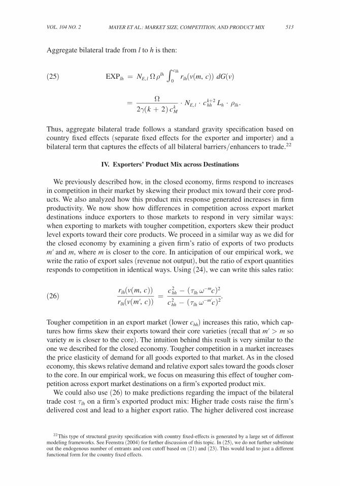
Aggregate bilateral trade from l to h is then:
(25) EX P lh = N E, l Ω ρ lh ∫ 0 c lh
r lh (v(m, c)) dG(v)
= Ω _ 2γ ( k + 2 ) c M k
⋅ N E, l ⋅ c hh k+2 L h ⋅ ρ lh .
Thus, aggregate bilateral trade follows a standard gravity specification based on country fixed effects (separate fixed effects for the exporter and importer) and a bilateral term that captures the effects of all bilateral barriers/enhancers to trade.22
IV. Exporters’ Product Mix across Destinations
We previously described how, in the closed economy, firms respond to increases in competition in their market by skewing their product mix toward their core prod-ucts. We also analyzed how this product mix response generated increases in firm productivity. We now show how differences in competition across export market destinations induce exporters to those markets to respond in very similar ways: when exporting to markets with tougher competition, exporters skew their product level exports toward their core products. We proceed in a similar way as we did for the closed economy by examining a given firm’s ratio of exports of two products m′ and m, where m is closer to the core. In anticipation of our empirical work, we write the ratio of export sales (revenue not output), but the ratio of export quantities responds to competition in identical ways. Using (24), we can write this sales ratio:
(26) r lh (v ( m, c ) )
_ r lh (v ( m′ , c ) )
= c hh 2
− ( τ lh ω −m c ) 2 __
c hh 2 − ( τ lh ω − m′ c ) 2
.
Tougher competition in an export market (lower c hh ) increases this ratio, which cap-tures how firms skew their exports toward their core varieties (recall that m′ > m so variety m is closer to the core). The intuition behind this result is very similar to the one we described for the closed economy. Tougher competition in a market increases the price elasticity of demand for all goods exported to that market. As in the closed economy, this skews relative demand and relative export sales toward the goods closer to the core. In our empirical work, we focus on measuring this effect of tougher com-petition across export market destinations on a firm’s exported product mix.
We could also use (26) to make predictions regarding the impact of the bilateral trade cost τ lh on a firm’s exported product mix: Higher trade costs raise the firm’s delivered cost and lead to a higher export ratio. The higher delivered cost increase
22 This type of structural gravity specification with country fixed-effects is generated by a large set of different modeling frameworks. See Feenstra (2004) for further discussion of this topic. In (25), we do not further substitute out the endogenous number of entrants and cost cutoff based on (21) and (23). This would lead to just a different functional form for the country fixed effects.

514 THE AMERICAN ECONOMIC REVIEW FEBRUARY 2014
the competition faced by an exporting firm, as it then competes against domestic firms that benefit from a greater cost advantage. However, this comparative static is very sensitive to the specification for the trade cost across a firm’s product ladder. If trade barriers induce disproportionately higher trade costs on products further away from the core, then the direction of this comparative static would be reversed. Furthermore, identifying the independent effect of trade barriers on the exporters’ product mix would also require micro-level data for exporters located in many dif-ferent countries (to generate variation across both origin and destination of export sales). Our data “only” covers the export patterns for French exporters, and does not give us this variation in origin country. For these reasons, we do not emphasize the effect of trade barriers on the product mix of exporters. In our empirical work, we will only seek to control for a potential correlation between bilateral trade barriers with respect to France and the level of competition in destination countries served by French exporters.23
As was the case for the closed economy, the skewing of a firm’s product mix toward core varieties also entails increases in firm productivity. Empirically, we cannot separately measure a firm’s productivity with respect to its production for each export market. However, we can theoretically define such a productivity measure in an analogous way to Φ(c) ≡ Q(c)/C(c) for the closed economy. We thus define the productivity of firm c in l for its exports to destination h as Φ lh (c) ≡ Q lh (c)/ C lh (c), where Q lh (c) are the total units of output that firm c exports to h, and C lh (c) are the total labor costs incurred by firm c to produce those units.24 In Appendix B, we show that this export market-specific productivity measure (as well as the associated measure Φ R, lh (c) based on deflated sales) increases with the toughness of competition in that export market. In other words, Φ lh (c) and Φ R, lh (c) both increase when c hh decreases. Thus, changes in exported product mix also have important repercussions for firm productivity.
V. Empirical Analysis
A. Skewness of Exported Product Mix
We now test the main prediction of our model regarding the impact of competi-tion across export market destinations on a firm’s exported product mix. Our model predicts that tougher competition in an export market will induce firms to lower markups on all their exported products and therefore skew their export sales toward their best performing products. We thus need data on a firm’s exports across prod-ucts and destinations. We use comprehensive firm-level data on annual shipments by all French exporters to all countries in the world for a set of more than 10,000 goods. Firm-level exports are collected by French customs and include export sales for each
23 The theoretical implications of our model for trade liberalization are discussed in Appendix A.24 In order for this productivity measure to aggregate up to overall country productivity, we incorporate the pro-
ductivity of the transportation/trade cost sector into this productivity measure. This implies that firm c employs the labor units that are used to produce the “melted” units of output that cover the trade cost; those labor units are thus included in C lh (c). The output of firm c is measured as valued-added, which implies that those “melted” units are not included in Q lh (c) (the latter are the number of units produced by firm c that are consumed in h). Separating out the productivity of the transportation sector would not affect our main comparative static with respect to toughness of competition in the export market.
515MAYER ET AL.: MARKET SIZE, COMPETITION, AND PRODUCT MIXVOL. 104 NO. 2
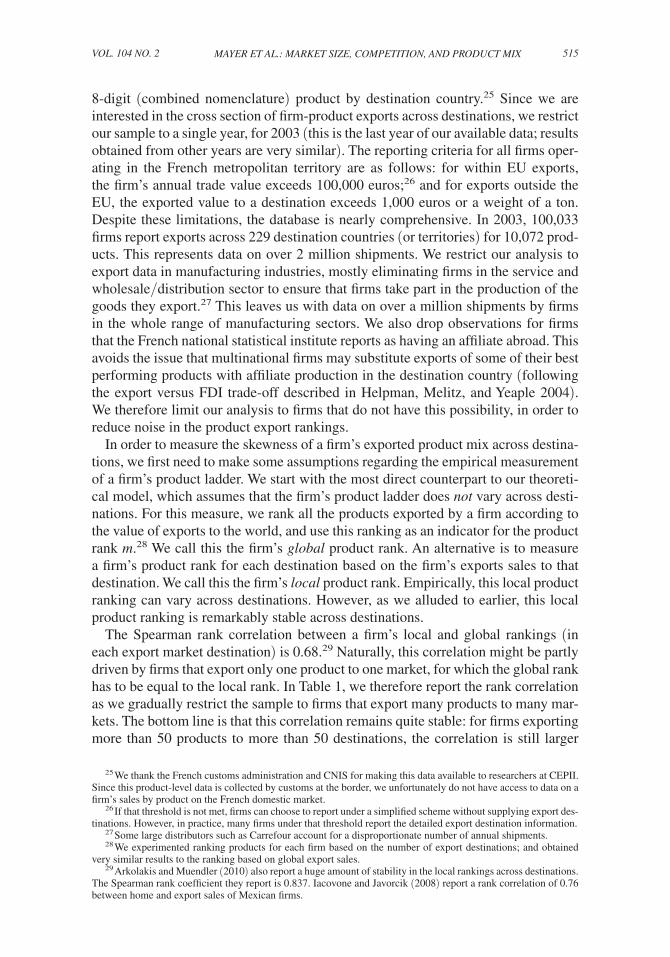
8-digit (combined nomenclature) product by destination country.25 Since we are interested in the cross section of firm-product exports across destinations, we restrict our sample to a single year, for 2003 (this is the last year of our available data; results obtained from other years are very similar). The reporting criteria for all firms oper-ating in the French metropolitan territory are as follows: for within EU exports, the firm’s annual trade value exceeds 100,000 euros;26 and for exports outside the EU, the exported value to a destination exceeds 1,000 euros or a weight of a ton. Despite these limitations, the database is nearly comprehensive. In 2003, 100,033 firms report exports across 229 destination countries (or territories) for 10,072 prod-ucts. This represents data on over 2 million shipments. We restrict our analysis to export data in manufacturing industries, mostly eliminating firms in the service and wholesale/distribution sector to ensure that firms take part in the production of the goods they export.27 This leaves us with data on over a million shipments by firms in the whole range of manufacturing sectors. We also drop observations for firms that the French national statistical institute reports as having an affiliate abroad. This avoids the issue that multinational firms may substitute exports of some of their best performing products with affiliate production in the destination country (following the export versus FDI trade-off described in Helpman, Melitz, and Yeaple 2004). We therefore limit our analysis to firms that do not have this possibility, in order to reduce noise in the product export rankings.
In order to measure the skewness of a firm’s exported product mix across destina-tions, we first need to make some assumptions regarding the empirical measurement of a firm’s product ladder. We start with the most direct counterpart to our theoreti-cal model, which assumes that the firm’s product ladder does not vary across desti-nations. For this measure, we rank all the products exported by a firm according to the value of exports to the world, and use this ranking as an indicator for the product rank m.28 We call this the firm’s global product rank. An alternative is to measure a firm’s product rank for each destination based on the firm’s exports sales to that destination. We call this the firm’s local product rank. Empirically, this local product ranking can vary across destinations. However, as we alluded to earlier, this local product ranking is remarkably stable across destinations.
The Spearman rank correlation between a firm’s local and global rankings (in each export market destination) is 0.68.29 Naturally, this correlation might be partly driven by firms that export only one product to one market, for which the global rank has to be equal to the local rank. In Table 1, we therefore report the rank correlation as we gradually restrict the sample to firms that export many products to many mar-kets. The bottom line is that this correlation remains quite stable: for firms exporting more than 50 products to more than 50 destinations, the correlation is still larger
25 We thank the French customs administration and CNIS for making this data available to researchers at CEPII. Since this product-level data is collected by customs at the border, we unfortunately do not have access to data on a firm’s sales by product on the French domestic market.
26 If that threshold is not met, firms can choose to report under a simplified scheme without supplying export des-tinations. However, in practice, many firms under that threshold report the detailed export destination information.
27 Some large distributors such as Carrefour account for a disproportionate number of annual shipments.28 We experimented ranking products for each firm based on the number of export destinations; and obtained
very similar results to the ranking based on global export sales.29 Arkolakis and Muendler (2010) also report a huge amount of stability in the local rankings across destinations.
The Spearman rank coefficient they report is 0.837. Iacovone and Javorcik (2008) report a rank correlation of 0.76 between home and export sales of Mexican firms.

516 THE AMERICAN ECONOMIC REVIEW FEBRUARY 2014
than 0.59. Another possibility is that this correlation is different across destination income levels. Restricting the sample to the top 50 or 20 percent richest import-ers hardly changes this correlation (0.69 and 0.71 respectively).30 Table 1 does not directly control for product selection, whereby any product that is not exported to a destination is dropped from the local ranking. Although we do not use this extensive margin response, we show in Appendix E that this product selection into the local ranking is also strongly correlated with the product’s global ranking for the firm: products with lower global ranking are exported to fewer destinations (on aver-age, the second ranked product is exported to around five fewer destinations; see Appendix E for details).
Although high, this correlation still highlights substantial departures from a steady global product ladder. A natural alternative is therefore to use the local prod-uct rank when measuring the skewness of a firm’s exported product mix. In this interpretation, the identity of the core (or other rank number) product can change across destinations. We thus use both the firm’s global and local product rank to con-struct the firm’s destination-specific export sales ratio r lh (v(m, c))/ r lh (v( m′ , c)) for m < m′ . Since many firms export few products to many destinations, increasing the higher product rank m′ disproportionately reduces the number of available firm/destination observations. For most of our analysis, we pick m = 0 (core prod-uct) and m′ = 1, but also report results for m′ = 2.31 Thus, we construct the ratio of a firm’s export sales to every destination for its best performing product (either globally, or in each destination) relative to its next best performing product (again, either globally, or in each destination). The local ratios can be computed so long as a firm exports at least two products to a destination (or three when m′ = 2). The global ratios can be computed so long as a firm exports its top (in terms of world exports) two products to a destination. We thus obtain these measures that are firm c and destination h specific, so long as those criteria are met (there is no variation in origin l = France). We use those ratios in logs, so that they represent percentage dif-ferences in export sales. We refer to the ratios as either local or global, based on the ranking method used to compute them. Lastly, we also constrain the sample so that the two products considered belong to the same 2-digit product category (there are
30 We nevertheless separately report our regression results for those restricted sample of countries based on income.
31 We also obtain very similar results for m = 1 and m′ = 2.
Table 1—Spearman Correlations between Global and Local Rankings
Firms exporting at least: Number of products ( percent)
To number of countries 1 2 5 10 50
1 67.61 67.47 66.93 65.92 59.392 67.58 67.45 66.93 65.93 59.395 67.47 67.39 66.93 65.95 59.4010 67.27 67.22 66.88 65.99 59.4650 64.48 64.48 64.41 64.12 59.30
517MAYER ET AL.: MARKET SIZE, COMPETITION, AND PRODUCT MIXVOL. 104 NO. 2
97 such categories). This eliminates ratios based on products that are in completely different sectors; however, this restriction hardly impacts our reported results.
We construct a third set of measures that seeks to capture changes in skewness of a firm’s exported product mix over the entire range of exported products (instead of being confined to the top two or three products). We use several different skewness statistics for the distribution of firm export sales to a destination: the standard devia-tion of log export sales, a Herfindhal index, and a Theil index (a measure of entropy). Since these statistics are independent of the identity of the products exported to a destination, they are “local” by nature, and do not have any global ranking counter-part. These statistics can be computed for every firm-destination combination where the firm exports two or more products.
As we discussed in the introduction, we focus our empirical analysis on the response of the exported product mix (intensive margin) and do not investigate our model’s prediction for the extensive margin across destinations. Empirically, the number of products exported is under-reported due to a minimum sales reporting threshold. Theoretically, the predictions for the response of the extensive margin is quite sensitive to the specification of fixed exporting costs (which could be either destination-specific, or product-destination-specific, or some combination of both). We abstract from these fixed costs in order to maintain the tractability of our model in an asymmetric multi-country setting.32 As we previously noted, fixed export costs affect the extensive margin responses; but conditional on a firm’s decision to export a given set of products, those costs would not affect our skewness measures for the firms’ exported product mix. Our main novel prediction concerns how this skewness varies across export market destinations.
B. Toughness of Competition across Destinations and Bilateral Controls
Our theoretical model predicts that the toughness of competition in a destination is determined by that destination’s size, and by its geography (proximity to other big countries). We control for country size using GDP expressed in a common currency at market exchange rates. We now seek a control for the geography of a destina-tion that does not rely on country-level data for that destination. We use the supply potential concept introduced by Redding and Venables (2004) as such a control. In words, the supply potential is the aggregate predicted exports to a destination based on a bilateral trade gravity equation (in logs) with both exporter and importer fixed effects and the standard bilateral measures of trade barriers/enhancers. We construct a related measure of a destination’s foreign supply potential that does not use the importer’s fixed effect when predicting aggregate exports to that destination. By construction, foreign supply potential is thus uncorrelated with the importer’s fixed-effect. It is closely related to the construction of a country’s market poten-tial (which seeks to capture a measure of predicted import demand for a country).
32 Absent fixed exporting costs, our theoretical model predicts that a given firm exports fewer products to desti-nations where competition is tougher. However, a given firm would still export more products above a given sales threshold to larger destinations, even though competition is tougher there. Empirically, we observe that French firms report exporting more products to larger destinations (higher GDP). This could be due in part to the reporting threshold for exports, but is also a likely indication that destination-specific fixed export costs play an important role in determining the extensive margin of trade.

518 THE AMERICAN ECONOMIC REVIEW FEBRUARY 2014
The construction of the supply potential measures is discussed in greater detail in Redding and Venables (2004); we use the foreign supply measure for the year 2003 from Head and Mayer (2011) who extend the analysis to many more countries and more years of data.33 Since we only work with the foreign supply potential measure, we drop the qualifier “foreign” when we subsequently refer to this variable. There are likely several other country characteristics that affect competition in a destina-tion. As a robustness check, we also use the number of French exporters to a des-tination as a measure of competition for French firms in that market; this measure combines the effects of both destination size and geography as well as other des-tination characteristics that impact the extent of competition for French exporters. Those robustness results are reported in Appendix D.
We also use a set of controls for bilateral trade barriers/enhancers (τ in our model) between France and the destination country: distance, contiguity, colonial links, common-language, and dummies for membership of Regional Trading Agreements, GATT/WTO, and a common currency area (the euro zone in this case).34
C. Results
Before reporting the regression results of the skewness measures on the destina-tion country measures, we first show some scatter plots for the global ratio against both destination country GDP and our measure of supply potential. These are dis-played in Figures 2 and 3. For each destination, we use the mean global ratio across exporting firms. Since the firm-level measure is very noisy, the precision of the mean increases with the number of available firm data points (for each destination). We first show the scatter plots using all available destinations, with symbol weights proportional to the number of available firm observations, and then again dropping any destination with fewer than 250 exporting firms.35 Those scatter plots show a very strong positive correlation between the export share ratios and the measures of toughness of competition in the destination. Absent any variation in the toughness of competition across destinations—such as in a world with monopolistic competition and CES preferences where markups are exogenously fixed—the variation in the relative export shares should be white noise. The data clearly show that variations in competition (at least as proxied by country size and supplier potential) are strong enough to induce large variations in the firms’ relative export sales across destina-tions. Scatter plots for the local ratio and Theil index look very similar.
We now turn to our regression analysis using the three skewness measures. Each observation summarizes the skewness of export sales for a given firm to a given destination. Since we seek to uncover variation in that skewness for a given firm, we include firm fixed effects throughout. Our remaining independent variables are destination specific: our two measures of competition (GDP and supplier potential, both in logs) as well as any bilateral measures of trade barriers/enhancers since
33 As is the case with market potential, a country’s supplier potential is strongly correlated with that country’s GDP: big trading economies tend to be located near one-another. The supply potential data is available online at http://www.cepii.fr/anglaisgraph/bdd/marketpotentials.htm.
34 All those variables are available at http://www.cepii.fr/anglaisgraph/bdd/gravity.htm.35 Increasing that threshold level for the number of exporters slightly increases the fit and slope of the regression
line through the scatter plot.

519MAYER ET AL.: MARKET SIZE, COMPETITION, AND PRODUCT MIXVOL. 104 NO. 2
there is no variation in country origin (we discuss how we specify those bilateral controls in further detail in the next paragraph). There are undoubtedly other unob-served characteristics of countries that affect our dependent skewness variables. These unobserved country characteristics are common to firms exporting to that destination and hence generate a correlated error-term structure, potentially biasing
Figure 2. Mean Global Ratio and Destination Country GDP in 2003
Figure 3. Mean Global Ratio and Destination Supply Potential in 2003
1
10
100
1,000
1
10
100
1,000M
ean
glob
al r
atio
5 10 15
Destination GDP (log)
AGO
ARE
ARG
AUSAUT
BEL
BEN
BFA
BGD
BGR
BHR
BLR
BRACAN
CHECHL
CHN
CIV
CMR
COG COL
CRI
CYP
CZE
DEU
DJI
DNK
DOM
DZA
ECU
EGY
ESP
EST
FIN
GAB
GBR
GHA
GIN
GRC
GTM
HKG
HRV
HTI
HUNIDN
IND
IRL
IRN
ISL
ISR
ITA
JOR
JPN
KAZ
KEN
KOR
KWTLBN
LBY
LKA
LTU
LUX
LVAMAR
MDG
MEX
MLIMLT
MRTMUS
MYS
NER
NGA
NLD
NOR
NZL
OMN
PAKPAN
PER
PHL
POL
PRT
QAT
ROMRUS
SAU
SEN
SGPSVKSVN
SWE
SYR
TCD
TGO
THATUN
TUR
TWN
UKR
URY
USAVEN
VNM
YEM
YUG
ZAF
Mea
n gl
obal
rat
io
6 8 10 12 14 16
Destination GDP (log)
All countries (209) Countries with more than 250 exporters (112)
1
10
100
1,000
1
10
100
1,000
Mea
n gl
obal
rat
io
Mea
n gl
obal
rat
io
All countries (209) Countries with more than 250 exporters (112)
12 14 16 18 20
Foreign supply potential (log)
AGO
ANT
ARE
ARG
AUSAUT
BEL
BEN
BFA
BGD
BGR
BHR
BLR
BRA CAN
CHECHL
CHN
CIV
CMR
COGCOL
CRI
CYP
CZE
DEU
DJI
DNK
DOM
DZA
ECU
EGY
ESP
EST
FIN
GAB
GBR
GHA
GIN
GRC
GTM
HKG
HRV
HTI
HUNIDN
IND
IRL
IRN
ISL
ISR
ITA
JOR
JPN
KAZ
KEN
KOR
KWTLBN
LBY
LKA
LTU
LVAMAR
MDG
MEX
MLI MLT
MRTMUS
MYS
NCLNER
NGA
NLD
NOR
NZL
OMN
PAKPAN
PER
PHL
POL
PRT
PYF
QAT
ROMRUS
SAU
SEN
SGPSPM
SVKSVN
SWE
SYR
TCD
TGO
THATUN
TUR
UKR
URY
USAVEN
VNM
YEM
YUG
ZAF
12 14 16 18 20
Foreign supply potential (log)
520 THE AMERICAN ECONOMIC REVIEW FEBRUARY 2014
downward the standard error of our variables of interest. The standard clustering procedure does not apply well here for two reasons: (i) the level of clustering is not nested within the level of fixed effects, and (ii) the number of clusters is quite small with respect to the size of each cluster. Harrigan and Deng (2010) encounter a simi-lar problem and use the solution proposed by Wooldridge (2006), who recommends to run country-specific random effects on firm-demeaned data, with a robust covari-ance matrix estimation. This procedure allows to account for firm fixed effects, as well as country-level correlation patterns in the error term. We follow this estimation strategy here and apply it to all of the reported results below.36
Our first set of results regresses our two main skewness measures (log export ratio of best to next best product for global and local product rankings) on destina-tion GDP and foreign supply potential. The coefficients, reported in columns 1 and 4 of Table 2, show a very significant impact of both country size and geography on the skewness of a firm’s export sales to that destination (we discuss the economic magnitude in further detail below). This initial specification does not control for any independent effect of bilateral trade barriers on the skewness of a firm’s exported product mix. Here, we suffer from the limitation inherent in our data that we do not observe any variation in the country of origin for all the export flows. This makes it difficult to separately identify the effects of those bilateral trade barriers from the destination’s supply potential. France is located very near to the center of the biggest regional trading group in the world. Thus, distance from France is highly correlated with good geography and hence a high supply potential for that destination: the correlation between log distance and log supply potential is 78 percent. Therefore, when we introduce all the controls for bilateral trade barriers to our specification, it is not surprising that there is too much co-linearity with the destination’s supply potential to separately identify the independent effect of the latter.37 These results are reported in columns 2 and 5 of Table 2. Although the coefficient for supply potential is no longer significant due to this co-linearity problem, the effect of coun-try size on the skewness of export sales remain highly significant. Other than coun-try size, the only other variable that is significant (at 5 percent or below) is the effect of a common currency: export sales to countries in the euro zone display vastly higher skewness. However, we must exercise caution when interpreting this effect. Due to the lack of variation in origin country, we cannot say whether this captures the effect of a common currency between the destination and France, or whether this is an independent effect of the euro.38
Although we do not have firm-product-destination data for countries other than France, bilateral aggregate data is available for the full matrix of origins-destinations in the world. Our theoretical model predicts a bilateral gravity relationship (25) that
36 We have experimented with several other estimation procedures to control for the correlated error structure: firm-level fixed effects with/without country clustering and demeaned data run with simple OLS. Those procedures highlight that it is important to account for the country-level error-term correlation. This affects the significance of the supply potential variable (as we highlight with our preferred estimation procedure). However, the p-values for the GDP variable are always substantially lower, and none of those procedures come close to overturning the significance of that variable.
37 As we mentioned, distance by itself introduces a huge amount of co-linearity with supply potential. The other bilateral trade controls then further exacerbate this problem (membership in the European Union is also strongly correlated with good geography and hence supply potential).
38 If this is a destination euro effect, then this would fit well with our theoretical prediction for the effect of tougher competition in euro markets on the skewness of export sales.

521MAYER ET AL.: MARKET SIZE, COMPETITION, AND PRODUCT MIXVOL. 104 NO. 2
can be exploited to recover the combined effect of bilateral trade barriers as a single parameter ( τ lh in our model). The only property of our gravity relationship that we exploit is that bilateral trade can be decomposed into exporter and importer fixed effects, and a bilateral component that captures the joint effect of trade barriers.39 We use the same bilateral gravity specification that we previously used to construct supply potential (again, in logs). We purge bilateral flows from both origin and des-tination fixed effects, to keep only the contribution of bilateral barriers to trade. This gives us an estimate for the bilateral log freeness of trade between all country pairs (ln ρ lh ).40 We use the subset of this predicted data where France is the exporting coun-try. Looking across destinations, this freeness of trade variable is still highly correlated
39 This property of gravity equations is not specific to our model. It can be generated by a very large class of models. Head and Mayer (2011) discuss all the different models that lead to a similar gravity decomposition.
40 Again, we emphasize that there is a very large class of models that would generate the same procedure for recovering bilateral freeness of trade.
Table 2—Global and Local Export Sales Ratio: Core (m = 0) Product to Second Best (m′ = 1) Product
Ratio of core to second product sales’ regressions
Global ratio Local ratio
(1) (2) (3) (4) (5) (6)
ln GDP 0.092*** 0.083*** 0.107*** 0.073*** 0.057*** 0.077***(0.013) (0.012) (0.010) (0.008) (0.005) (0.006)
ln supply potential 0.067*** −0.017 0.044*** 0.080*** 0.018 0.068 ***(0.016) (0.024) (0.014) (0.016) (0.016) (0.013)
ln distance −0.063 −0.046*(0.043) (0.023)
Contiguity 0.013 −0.108(0.051) (0.081)
Colonial link −0.060 −0.041(0.051) (0.043)
Common language 0.023 −0.048(0.050) (0.038)
RTA 0.066 0.004(0.059) (0.033)
Common currency 0.182*** 0.335***(0.047) (0.036)
Both in GATT 0.006 −0.033(0.046) (0.026)
ln freeness of trade 0.096*** 0.028(0.026) (0.017)
Constant −0.000 0.000 −0.000 0.003 0.002 0.002(0.016) (0.012) (0.014) (0.012) (0.011) (0.013)
Observations 56,097 56,097 56,093 96,891 96,891 96,878Within R2 0.004 0.006 0.005 0.007 0.011 0.007
Notes: All columns use Wooldridge’s (2006) procedure: country-specific random effects on firm-demeaned data, with a robust covariance matrix estimation. Standard errors in parentheses.
*** Significant at the 1 percent level. ** Significant at the 5 percent level. * Significant at the 10 percent level.

522 THE AMERICAN ECONOMIC REVIEW FEBRUARY 2014
with distance from France (the correlation with log distance is 60 percent); but it is substantially less correlated with the destination’s supply potential than distance from France (the correlation between freeness of trade and log supply potential is 40 per-cent, much lower than the 78 percent correlation between log distance and log supply potential). This greatly alleviates the co-linearity problem while allowing us to con-trol for the relevant variation induced by bilateral trade barriers (i.e., calculated based upon their impact on bilateral trade flows).
Columns 3 and 6 of Table 2 report the results using this constructed freeness of trade measure as our control for the independent effect of bilateral trade barriers on export skewness. The results are very similar to our initial ones without any bilateral controls: country size and supply potential both have a strong and highly significant effect on the skewness of export sales. These effects are also economically sig-nificant. The coefficient on country size can be directly interpreted as an elasticity for the sales ratio with respect to country GDP. The 0.107 elasticity for the global ratio implies that an increase in destination GDP from that of the Czech Republic to German GDP (an increase from the seventy-ninth to ninety-ninth percentile in the world’s GDP distribution in 2003) would induce French firms to increase their relative exports of their best product (relative to their next best global product) by 42.1 percent: from an observed mean ratio of 20 in 2003 to 28.4.
We now investigate the robustness of this result to different skewness measures, to the sample of destination countries, and to an additional control for destination GDP per capita. From here on out, we use our constructed freeness of trade measure to control for bilateral trade barriers.
We report the same set of results for the global sales ratio in Table 3 and for the local ratio in Table 4. The first column reproduces baseline estimation reported in columns 3 and 6 with the freeness of trade control. In column 2, we use the sales ratio of the best to third best product as our dependent skewness variable.41 We then return to sales ratio based on best to next best for the remaining columns. In order to show that our results are not driven by unmeasured quality differences between the products shipped to developed and developing countries, we progressively restrict our sample of country destinations to a subset of richer countries. In column 3 we restrict destinations to those above the median country income, and in column 4, we only keep the top 20 percent of countries ranked by income (GDP per capita).42 In the fifth and last column, we keep the full sample of country destinations and add destination GDP per capita as a regressor in order to directly control for differences in preferences across countries (outside the scope of our theoretical model) tied to product quality and consumer income.43 All of these different specifications in
41 We also experimented with the ratio for the second best to third best product, and obtained very similar results.42 Since French firms ship disproportionately more goods to countries with higher incomes, the number of obser-
vations drops very slowly with the number of excluded country destinations.43 In particular, we want to allow consumer income to bias consumption toward higher quality varieties. If
within-firm product quality is negatively related to its distance from the core product, then this would induce a posi-tive correlation between consumer income and the within-firm skewness of expenditure shares. This is the sign of the coefficient on GDP per capita that we obtain; that coefficient is statistically significant for the regressions based on the local product ranking.

523MAYER ET AL.: MARKET SIZE, COMPETITION, AND PRODUCT MIXVOL. 104 NO. 2
Tables 3 and 4 confirm the robustness of our baseline results regarding the strong impact of both country size and geography on the firms’ export ratios.44
Lastly, we show that this effect of country size and geography on export skewness is not limited to the top 2–3 products exported by a firm to a destination. We now use our different statistics that measure the skewness of a firm’s export sales over the entire range of exported products. The first three columns of Table 5 use the standard
44 When we restrict the sample of destinations to the top 20 percent of richest countries, then our co-linearity problem resurfaces between the supply potential and freeness of trade measures, and the coefficient on supply potential is no longer statistically significant at the 5 percent level (only at the 10 percent level).
Table 3—Global Export Sales Ratio: Core Product (m = 0) to Product m′
(1) (2) (3) (4) (5)
ln GDP 0.107*** 0.131*** 0.110*** 0.096*** 0.098***(0.010) (0.010) (0.011) (0.012) (0.011)
ln supply potential 0.044*** 0.038** 0.038*** 0.022* 0.036**(0.014) (0.016) (0.014) (0.012) (0.016)
ln freeness of trade 0.096*** 0.085** 0.113*** 0.137*** 0.092***(0.026) (0.033) (0.032) (0.038) (0.026)
ln GDP per cap 0.025(0.018)
m′ = 1 2 1 1 1Destination GDP/cap all all top 50% top 20% allObservations 56,093 22,576 50,623 40,964 56,093Within R2 0.005 0.006 0.004 0.002 0.005
Notes: All columns use Wooldridge’s (2006) procedure: country-specific random effects on firm-demeaned data, with a robust covariance matrix estimation. Standard errors in parentheses.
*** Significant at the 1 percent level. ** Significant at the 5 percent level. * Significant at the 10 percent level.
Table 4—Local Export Sales Ratio: Core Product (m = 0) to Product m′
(1) (2) (3) (4) (5)
ln GDP 0.077*** 0.100*** 0.083*** 0.061*** 0.066***(0.006) (0.012) (0.011) (0.016) (0.008)
ln supply potential 0.068*** 0.064*** 0.051*** 0.028* 0.057***(0.013) (0.022) (0.018) (0.016) (0.014)
ln freeness of trade 0.028 0.013 0.059 0.092* 0.025(0.017) (0.042) (0.039) (0.052) (0.017)
ln GDP per cap 0.029**(0.013)
m′ = 1 2 1 1 1Destination GDP/cap all all top 50% top 20% allObservations 96,878 49,554 84,708 64,653 96,878Within R2 0.007 0.009 0.005 0.002 0.007
Notes: All columns use Wooldridge’s (2006) procedure: country-specific random effects on firm-demeaned data, with a robust covariance matrix estimation. Standard errors in parentheses.
*** Significant at the 1 percent level. ** Significant at the 5 percent level. * Significant at the 10 percent level.
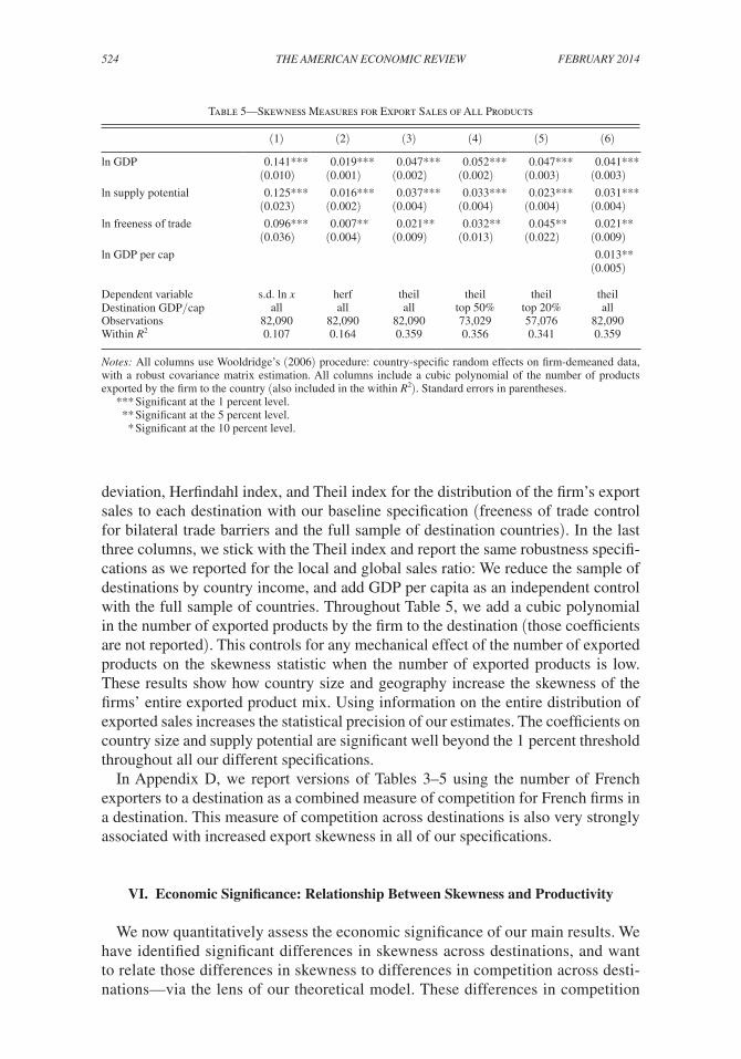
524 THE AMERICAN ECONOMIC REVIEW FEBRUARY 2014
deviation, Herfindahl index, and Theil index for the distribution of the firm’s export sales to each destination with our baseline specification (freeness of trade control for bilateral trade barriers and the full sample of destination countries). In the last three columns, we stick with the Theil index and report the same robustness specifi-cations as we reported for the local and global sales ratio: We reduce the sample of destinations by country income, and add GDP per capita as an independent control with the full sample of countries. Throughout Table 5, we add a cubic polynomial in the number of exported products by the firm to the destination (those coefficients are not reported). This controls for any mechanical effect of the number of exported products on the skewness statistic when the number of exported products is low. These results show how country size and geography increase the skewness of the firms’ entire exported product mix. Using information on the entire distribution of exported sales increases the statistical precision of our estimates. The coefficients on country size and supply potential are significant well beyond the 1 percent threshold throughout all our different specifications.
In Appendix D, we report versions of Tables 3–5 using the number of French exporters to a destination as a combined measure of competition for French firms in a destination. This measure of competition across destinations is also very strongly associated with increased export skewness in all of our specifications.
VI. Economic Significance: Relationship Between Skewness and Productivity
We now quantitatively assess the economic significance of our main results. We have identified significant differences in skewness across destinations, and want to relate those differences in skewness to differences in competition across desti-nations—via the lens of our theoretical model. These differences in competition
Table 5—Skewness Measures for Export Sales of All Products
(1) (2) (3) (4) (5) (6)
ln GDP 0.141*** 0.019*** 0.047*** 0.052*** 0.047*** 0.041***(0.010) (0.001) (0.002) (0.002) (0.003) (0.003)
ln supply potential 0.125*** 0.016*** 0.037*** 0.033*** 0.023*** 0.031***(0.023) (0.002) (0.004) (0.004) (0.004) (0.004)
ln freeness of trade 0.096*** 0.007** 0.021** 0.032** 0.045** 0.021**(0.036) (0.004) (0.009) (0.013) (0.022) (0.009)
ln GDP per cap 0.013**(0.005)
Dependent variable s.d. ln x herf theil theil theil theilDestination GDP/cap all all all top 50% top 20% allObservations 82,090 82,090 82,090 73,029 57,076 82,090Within R2 0.107 0.164 0.359 0.356 0.341 0.359
Notes: All columns use Wooldridge’s (2006) procedure: country-specific random effects on firm-demeaned data, with a robust covariance matrix estimation. All columns include a cubic polynomial of the number of products exported by the firm to the country (also included in the within R2). Standard errors in parentheses.
*** Significant at the 1 percent level. ** Significant at the 5 percent level. * Significant at the 10 percent level.

525MAYER ET AL.: MARKET SIZE, COMPETITION, AND PRODUCT MIXVOL. 104 NO. 2
are important because tougher competition induces an aggregate increase in productivity—holding technology fixed. In a closed economy, we showed in Appendix B how firm productivity—measured either as output per worker Φ(c) or deflated sales per worker Φ R (c)—increases when competition increases (the cutoff c D decreases). This effect holds even when the firm’s product range M(c) does not change, as it is driven by the increased skewness in the product mix (toward the best performing products). In the same Appendix, we also define par-allel measures of firm productivity Φ lh (c) and Φ R, lh (c) for the bundle of products exported by firm c from l to h. Similarly, these productivity measures increase with competition in that destination (lower c hh ) due to the same intra-firm real-locations across products driven by the increase in skewness. Since our avail-able data does not include measures of firm productivity, we must rely on the functional forms of our theoretical model to quantitatively relate export skew-ness to competition and productivity. This represents a significant departure from our empirical approach up to this point, which has avoided relying on those functional forms.
In Section II, we defined aggregate productivity _ Φ and
_ Φ R as the aggregate coun-
terparts to Φ(c) and Φ R (c), and showed that both aggregate measured were identi-cal, and inversely related to the cost cutoff. This describes the overall response of productivity to changes in the toughness of competition in the closed economy. We define the aggregate productivity for all products exported from l to h in a similar way:
_ Φ lh and
_ Φ R, lh are the aggregate counterparts to the firm productivity measures
Φ lh (c) and Φ R, lh (c). In Appendix C, we show that these two alternate measures coincide ( just like they do for aggregate productivity in the closed economy) and are inversely proportional to the cost cutoff c hh (the toughness of competition in the export destination). Thus, our theoretical model predicts that increases in the toughness of competition in a destination—measured as percentage decreases in the destination cutoff—lead to proportional increases in aggregate productiv-ity (same percentage change as the cutoff). This aggregate productivity response combines the effects of skewness on firm productivity, holding the product range fixed, as well as reallocation effects across products when the number of products changes, and reallocation effects across firms. However, because product market shares continuously drop to zero as competition toughens, the contribution of the product extensive margin (adding/dropping products) to productivity changes is second order, while the contribution of product skewness to productivity changes is first order. Thus, the unit elasticity between productivity and toughness of com-petition is driven by the effects of competition on product skewness. This is the key new channel that we emphasize in this paper.
Our main results in the previous section have quantified the link between observable country characteristics and export skewness. In particular, we have shown how differences in GDP induce significant differences in skewness for French exporters. We now quantitatively determine what differences in compe-tition (across countries) would yield those same observed differences in export skewness. This allows us to associate differences in competition with the differ-ences in GDP, in terms of their effect on the skewness of exports. In our theo-retical model, the relationship between competition in a destination (the cutoff c hh ) and export skewness for firm c from l (measured as the ratio of a firm’s

526 THE AMERICAN ECONOMIC REVIEW FEBRUARY 2014
exports of its core product, m = 0, to its next best performing product, m′ = 1) is given by (26):
(27) r r lh (c) = r lh (v ( m, c ) )
_ r lh (v ( m′ , c ) )
= ( c hh ) 2 − ( τ lh c ) 2
__ ( c hh ) 2 − ( τ lh c/ω ) 2
.
Our results in Tables 3 and 4 measure the average elasticity of this skewness measure with respect to destination h GDP—across all French exporters that export their top two products (global or local definition) to h. Using (27), we compute the average elasticity of this skewness measure with respect to competition in h (the cutoff c hh ):
_
d ln r r lh _ d ln c hh
= −2k 1 − ω 2 _ ω 2
( c hh τ lh ) 2
_ ( ω 2 c hh / τ lh ) k
∫ 0 ω 2 c hh / τ lh
c k+1 ___ [ c hh 2
− ( τ lh c ) 2 ] [ c hh 2 − ( τ lh c/ω ) 2 ]
dc
= −2k 1 − ω 2 _ ω 2k
∫ 0 ω 2
x k+1 __ ( 1 − x 2 ) ( ω 2 − x 2 )
dx, where x ≡ ( τ lh / c hh ) c ∈ [0, ω 2 ]
≡ f (ω, k).
Here, we have averaged over all firms in l selling at least three products to h as the elasticity is not defined for some firms exporting two products, who become single product exporters when the cutoff c hh decreases. We note that this average elasticity can be written as a function of just two model parameters: ω (the ladder step size), and k (the shape of the Pareto distribution for cost/productivity). We thus need empirical estimates of just those two coefficients. Several papers have estimated the Pareto shape coefficients k. Crozet and Koenig (2010) estimate a range for k between 1.34 and 4.43 for French exporters (by sector) while Eaton, Kortum, and Kramarz (2011) estimate k = 4.87 for all French firms. This range coincides well with estimates from other countries: Corcos et al. (2012) estimate k = 1.79 across European firms, and Bernard et al. (2003) estimate k = 3.6 for US firms. We report estimates of f ( ω , k ) for k between 1.34 and 4.87.
In order to estimate ω , we use our theoretical model to derive an estimation equa-tion for ϑ ≡ k ln ω based on our product-destination export data (see Appendix C). This yields a very precise estimate for ϑ, ϑ = −0.13, which we use to recover ω , given a choice for k . Given the small standard error for ϑ , differences in ω will be driven by our choice of k ; however, any alternate assumption for ϑ will have the same effect on ω as a proportional change in k . This completes our empiri-cal derivation for the average elasticity of skewness with respect to competition, __
d ln r r lh /d ln c hh ≡ f (ω, k). This elasticity ranges from 0.635 for k = 1.34 to 2.34 for k = 4.87 ; it is 1.52 at the midpoint for k = 3.11.
With estimates of this elasticity in hand, we can evaluate the economic signifi-cance of our previous results from Tables 3 and 4. In those tables, we reported an average elasticity of skewness to country GDP between 0.06 and 0.11. Dividing those elasticities by our estimate for
__ d ln r r lh /d ln c hh yields the change in com-
petition that would induce the same change in skewness as a doubling of country GDP. In our theoretical model, those changes in competition are proportional to
527MAYER ET AL.: MARKET SIZE, COMPETITION, AND PRODUCT MIXVOL. 104 NO. 2
changes in aggregate productivity for the bundle of goods sold in that destination. Viewed through this lens, the economic impact of the changes in skewness are quite large. For a doubling of country GDP, they imply changes in productivity between 2.56 percent and 17.3 percent. At our midpoint for k , the implied productivity changes are between 3.95 percent and 7.24 percent.
VII. Conclusion
In this paper, we have developed a model of multi-product firms that highlights how differences in market size and geography affect the within-firm distribution of export sales across destinations. This effect on the firms’ product mix choice is driven by variations in the toughness of competition across markets. Tougher com-petition induces a downward shift in the distribution of markups across all products, and increases the relative market share of the better performing products. We test these predictions for a comprehensive set of French exporters, and find that market size and geography indeed have a very strong impact on their exported product mix across world destinations: French firms skew their export sales toward their better performing products in big destination markets, and markets where many exporters from around the world compete (high foreign supply potential markets). We have obtained these results without imposing the specific functional forms (for demand, for the geometric product ladder, and for the Pareto inverse cost draws) that we used in our theoretical model. We therefore view our results as giving a strong indication of substantial differences in competition across export markets—rather than provid-ing goodness of fit test to our specific model (and its functional forms). We cannot measure markups directly but the strong link between tougher competition and a more skewed product mix is suggestive of substantial markup adjustments by export-ers across destinations. In any event, trade models based on exogenous markups can-not explain this strong significant link between destination market characteristics and the within-firm skewness of export sales (after controlling for bilateral trade costs).
Theoretically, we showed how such an increase in skewness toward better perform-ing products (driven by tougher competition) would also be reflected in higher firm productivity. We cannot directly test this link without productivity data. Instead, we have leaned more heavily on the functional forms of our theoretical model. A cali-brated fit to that model reveals that these productivity effects are potentially quite large.
Appendix
A. Trade Liberalization
In this Appendix, we briefly discuss the predictions of our model regarding trade liberalization (unilateral and multilateral) in the context of a two country version of our model. The main message is that the effects of trade liberalization on aggregate variables (competition, productivity, welfare) are identical to those analyzed in Melitz and Ottaviano (2008) in the context of single-product firms. However, our current model allows us to translate those aggregate changes into predictions for the responses of multi-product firms. The main link is the one we have emphasized (both

528 THE AMERICAN ECONOMIC REVIEW FEBRUARY 2014
theoretically and empirically) in the cross section of destinations: how changes in competition lead to associated changes in the multi-product firms’ product mix and hence to changes in their productivity. In this respect, the predictions are starkly dif-ferent than the case of single-product firms where productivity (output per worker) is exogenously fixed independently of the competitive environment.
Equation (21) summarizes the effect of trade costs on competition in every mar-ket (the resulting cost cutoff c hh ) via the matrix of trade freeness P = [ ρ lh ] where ρ lh ≡ τ lh −k < 1. In a two country world, this simplifies to:
(A1) c hh = ( 1 − ρ hl _ 1 − ρ hl ρ lh
γϕ _
Ω L h )
1 _ k+2
, l ≠ h.
Equation (22) then expresses the resulting product variety in country h as a function of that cutoff. The determination of the cutoff in (A1) is very similar to the case of single-product firms: this is the case where Ω = 1. Trade liberalization thus induces a similar response as in the single-product case. Bilateral trade liberalization (higher ρ lh and ρ hl ) increases competition in both countries (lower cutoffs c hh and c ll ). On the other hand, unilateral trade liberalization in country h (higher ρ lh with ρ hl remaining unchanged) results in weaker competition in h (higher c hh ) and tougher competition in its trading partner l (lower c ll ). This divergence is due to the impact of the asym-metric liberalization on the firms’ entry decisions: unilateral trade liberalization by h increases the incentives for entry in its trading partner l; entry in h is reduced, while entry in l increases. We can also define a short-run equilibrium in a similar way to the one defined for single-product firms in Melitz and Ottaviano (2008). With entry fixed in the short run, unilateral trade liberalization will then increase competition in the liberalizing country, due to the increase in import competition (in the long run, the increase in import competition is more than offset by the effects of exit). An analysis of preferential trade liberalization would also lead to similar results on competition as those described in Melitz and Ottaviano (2008).
B. Tougher Competition and Firm Productivity
In Section II we argued that tougher competition induces improvements in firm productivity through its impact on a firm’s product mix. Here we show that both firm productivity measures, output per worker Φ(c) and deflated sales per worker Φ R (c), increase for all multi-product firms when competition increases ( c D decreases). We provide proofs for the closed as well as the open economy. In both cases we proceed in two steps. First, we show that, holding a firm’s prod-uct scope constant, firm productivity over that product scope increases whenever competition increases. Then, we extend the argument by continuity to cover the case where tougher competition induces a change in product scope.
Closed Economy.—Consider a firm with cost c producing M(c) varieties. Output per worker is given by
Φ(c) = Q(c) _
C(c) =
∑ m=0 M(c)−1 q ( v ( m, c ) )
__ ∑ m=0
M(c)−1 v ( m, c ) q ( v ( m, c ) ) =
L _ 2γ ∑ m=0 M(c)−1 ( c D − ω −m c )
__ L _ 2γ ∑ m=0
M(c)−1 ω −m ( c D − ω −m c ) .

529MAYER ET AL.: MARKET SIZE, COMPETITION, AND PRODUCT MIXVOL. 104 NO. 2
For a fixed product scope M with 1 < M ≤ M(c), this can be written as
(B1) Φ(c) = ω M ( 1 − ω )
_ ω ( 1 − ω M )
M _ c c D − c _ M
ω ( 1 − ω M ) _
ω M ( 1 − ω ) __
c D − c ω ( 1 + ω M )
_ ω M ( 1 + ω )
,
subject to c ∈ [ c D ω M , c D ω M−1 ]. Differentiating (B1) with respect to c D implies that
dΦ(c) _
d c D < 0 ⇔ c
ω ( 1 + ω M ) _
ω M ( 1 + ω ) > c _
M ω ( 1 − ω M )
_ ω M ( 1 − ω )
or, equivalently, if and only if
(B2) M > ( 1 + ω ) ( 1 − ω M )
__ ( 1 + ω M ) ( 1 − ω )
.
This is always the case for M > 1: the left- and right-hand sides are identical for M = 0 and M = 1, and the right-hand side is increasing and concave in M. This proves that, holding M > 1 constant, a firm’s output per worker is larger in a market where competition is tougher (lower c D ).
Even when product scope M drops due to the decrease in c D , output per worker must still increase due to the continuity of Φ(c) with respect to c D (both Q(c) and C(c) are continuous in c D as the firm produces zero units of a variety right before it is dropped when competition gets tougher). To see this, consider a large down-ward change in the cutoff c D . The result for given M tells us that output per worker for a firm with given c increases on all ranges of c D where the number of varieties produced does not change. This just leaves a discrete number of c D s where the firm changes the number of products produced. Since Φ(c) is continuous at those c D s, and increasing everywhere else, it must be increasing everywhere.
The unavailability of data on physical output often leads to a measure of produc-tivity in terms of deflated sales per worker. Over the fixed product scope M with 1 < M ≤ M(c), this alternate productivity measure is defined as
(B3) Φ R (c) = R(c)/
_ P _
C(c) = 1 _
2 k + 2
_ k + 1
1 _ c D M ( c D ) 2 − c 2 ω 2 1 − ω 2 M __
ω 2 M ( 1 − ω ) ( 1 + ω ) ___
c D cω 1 − ω M _ ω M ( 1 − ω )
− c 2 ω 2 1 − ω 2 M __ ω 2M ( 1 − ω ) ( 1 + ω )
,
subject to c ∈ [ c D ω M , c D ω M−1 ]. Differentiating (B3) with respect to c D then yields
d ( R(c)/
_ P _
C(c) ) _
d c D = − 1 _
2 k + 2
_ k + 1
1 + ω M
_ 1 − ω M
⋅
M ω 2M ( 1 − ω 2 ) ( c D ) 2 − 2c ω M+1 ( 1 + ω ) ( 1 − ω M ) c D + c 2 ω 2 ( 1 − ω 2 M )
_____ ( c D ) 2 [ ω M ( 1 + ω ) c D − cω ( 1 + ω M ) ] 2
< 0.

530 THE AMERICAN ECONOMIC REVIEW FEBRUARY 2014
Here, we have used the fact that c ∈ [ c D ω M , c D ω M−1 ] implies
M ω 2M ( 1 − ω 2 ) ( c/ ω M ) 2 − 2c ω M+1 ( 1 + ω ) ( 1 − ω M ) ( c/ ω M ) > 0.
This proves that, holding M > 1 constant, this alternative productivity measure Φ R (c) also increases when competition is tougher (lower c D ). The same reasoning applies to the case where tougher competition induces a reduction in product scope M.
Note that, in the special case of M = 1, we have
Φ R (c) = 1 _ 2
k + 2 _
k + 1 ( 1 _ c + 1 _ c D ) .
Hence, whereas tougher competition (lower c D ) has no impact on the output per worker Φ(c) of a single-product firm, it still raises deflated sales per worker Φ R (c). This is due to the fact that deflated sales per worker are also affected by markup changes when the toughness of competition changes.
Open Economy.—Consider a firm with cost c selling M lh (c) varieties from coun-try l to country h. Exported output per worker is given by
Φ lh (c) ≡ Q lh (c) _ C lh (c)
= ∑ m=0
M lh (c)−1 c hh − τ lh ω −m c ___
∑ m=0 M lh (c)−1 ( τ lh ω −m c ) ( c hh − τ lh ω −m c )
.
For a fixed product scope M with 1 < M ≤ M lh (c), this can be written as
(B4) Φ lh (c) = ω M ( 1 − ω )
_ ω ( 1 − ω M )
M _ c τ lh c hh − c τ lh _ M
ω ( 1 − ω M ) _
ω M ( 1 − ω ) __
c hh − c τ lh ω ( 1 + ω M )
_ ω M ( 1 + ω )
,
subject to c τ lh ∈ [ c hh ω M , c hh ω M−1 ]. Differentiating (B4) with respect to c hh yields
d Φ lh (c) _
d c hh < 0 ⇔ c τ lh
ω ( 1 + ω M ) _
ω M ( 1 + ω ) >
c τ lh _ M
ω ( 1 − ω M )
_ ω M ( 1 − ω )
.
This must hold for M > 1 (see (B2)). Hence, tougher competition (lower c hh ) in the destination market increases exported output per worker. As in the closed economy, the fact that output per worker is continuous at a discrete number of c hh s and decreas-ing in c hh everywhere else implies that it is decreasing in c hh everywhere.
We now turn to productivity measured as deflated export sales per worker. Over the fixed product scope M with 1 < M ≤ M(c), this is defined as
(B5) Φ R, lh (c) = R lh (c)/
_ P h _
C lh (c)
= 1 _ 2 k + 2
_ k + 1
1 _ c hh
M ( c hh ) 2 − c 2 ( τ lh ) 2 ω 2 1 − ω 2M __ ω 2M ( 1 − ω ) ( 1 + ω )
____
c hh c τ lh ω 1 − ω M _ ω M ( 1 − ω )
− c 2 ( τ lh ) 2 ω 2 1 − ω 2M __ ω 2M ( 1 − ω ) ( 1 + ω )
,
531MAYER ET AL.: MARKET SIZE, COMPETITION, AND PRODUCT MIXVOL. 104 NO. 2
subject to c τ lh ∈ [ c hh ω M , c hh ω M−1 ]. Differentiating (B5) with respect to c hh yields
d Φ R, lh (c) _
d c hh = − 1 _
2 k + 2
_ k + 1
1 + ω M
_ 1 − ω M
⋅
M ω 2M ( 1 − ω 2 ) ( c hh ) 2 − 2c τ lh ω M+1 ( 1 + ω ) ( 1 − ω M ) c hh + c 2 ( τ lh ) 2 ω 2 ( 1 − ω 2M )
______ ( c hh ) 2 [ ω M ( 1 + ω ) c hh − c τ lh ω ( 1 + ω M ) ] 2
< 0.
The last inequality holds since c τ lh ∈ [ c hh ω M , c hh ω M−1 ] implies
M ω 2M ( 1 − ω 2 ) ( c τ lh / ω M ) 2 − 2c τ lh ω M+1 ( 1 + ω ) ( 1 − ω M ) ( c τ lh / ω M ) > 0.
This proves that, holding M > 1 constant, productivity measured as deflated export sales per worker increases with tougher competition in the export market (lower c hh ). The same applies to the case where the tougher competition induces a response in the exported product scope M, as Φ R, lh (c) is continuous in c hh .
C. Calibration of Relationship between Skewness and Productivity
Aggregate Productivity Index for Bundle of Exported Goods.—In the previous Appendix section, we defined productivity indices for firm’s c bundle of exported goods from l to h as the output per worker associated with that bundle of exports:
Φ lh (c) ≡ Q lh (c) _ C lh (c)
and Φ R, lh (c) = R lh (c)/
_ P h _
C lh (c) ,
where the R subscript are productivity measures based on deflated sales as a mea-sure of firm output. The aggregate counterparts for all bilateral exports from l to h are just the same measures of output per worker computed for the aggregate bundle of exported goods:
_ Φ lh ≡
∫ 0 ω m c hh / τ lh
Q lh (c) dG(c) __
∫ 0 ω m c hh / τ lh
C lh (c) dG(c) = k + 2
_ k 1 _ c hh
,
_ Φ R, lh ≡
[ ∫ 0 ω m c hh / τ lh
R lh (c) dG(c) ] / _ P h __
∫ 0 ω m c hh / τ lh
C lh (c) dG(c) = k + 2
_ k 1 _ c hh
.
Just like the case of aggregate productivity in the closed economy, our two aggregate productivity measures overlap and are inversely proportional to the cutoff c hh in the export destination h.

532 THE AMERICAN ECONOMIC REVIEW FEBRUARY 2014
Estimating the Product Ladder Step Size ω.—We obtain an estimating equation for the ladder step size ω by aggregating all the product export sales across firms (for bilateral exports from l to h) that are at the same ladder step m:
R lh (m) = ∫ 0 c hh /( τ lh ω −m )
R lh (c, m) d ( c _ c M ) k = [ L _ γ ( k + 2 )
( c hh ) k+2
_ ( τ lh c M ) k
] ω km .
Thus, R lh (0) represents aggregate exports of core products from l to h ; R lh (1) for the second best performing product, and so forth for the product that is m steps from the core product. This implies a linear relationship between the log of product export sales ln R lh (m) and its associated ladder step m, with a slope given by ϑ ≡ k ln ω and an intercept that varies across bilateral country pairs. We can easily compute R lh (m) from our data by aggregating firm-product export sales from France to any destination h—across all products at the same ladder step m. A linear regression of ln R lh (m) on m with destination h fixed effects (capturing the term in the brackets) will then yield our estimate for ϑ (origin country l is held fixed for France).
We visually summarize this regression in Figure C1, where we have eliminated the destination fixed-effects by demeaning the export sales ln R lh (m) and the asso-ciated product m by destination h. By construction, this regression must deliver a negative fitted line. However, Figure C1 also clearly reveals that the linear rela-tionship provides an excellent fit. The figure also reveals that our slope coeffi-cient ϑ = −0.13 is very tightly estimated, with no appreciable slope variation within a 99 percent confidence interval.
−15
−10
−5
0
5
10
−50 −40 −30 −20 −10 0 10 20 30 40 50
Rank of product (country-demeaned)
log sales (country-demeaned)
fitted (β = −0.13)
fitted (1% lower bound of β)
fitted (1% upper bound of β)
Figure C1. Regression Yielding Estimate of ϑ

533MAYER ET AL.: MARKET SIZE, COMPETITION, AND PRODUCT MIXVOL. 104 NO. 2
D. Robustness to Alternate Measure of Toughness of Competition
As we mentioned in the main text, we repeat our main estimation procedures using the number of French exporters to a destination as a combined measure of the toughness of competition (for French firms) in a destination. We begin by showing the scatter plots of the mean global ratio plotted against this alternate competition measure (direct parallel to Figures 2 and 3). Figure D1 clearly shows that there is also a very strong increasing relationship between the global ratio and this alternate measure of competition.
1
10
100
1,000M
ean
glob
al r
atio
1
10
100
1,000
Mea
n gl
obal
rat
io
1 10 100 1,000 10,000
Count of French exporters (log scale)
AGO
ANDANT
ARE
ARG
AUSAUT
BEL
BEN
BFA
BGD
BGR
BHR
BLR
BRA CAN
CHECHL
CHN
CIV
CMR
COGCOL
CRI
CYP
CZE
DEU
DJI
DNK
DOM
DZA
ECU
EGY
ESP
EST
FIN
GAB
GBR
GHA
GIN
GRC
GTM
HKG
HRV
HTI
HUNIDN
IND
IRL
IRN
ISL
ISR
ITA
JOR
JPN
KAZ
KEN
KOR
KWTLBN
LBY
LKA
LTU
LUX
LVAMAR
MDG
MEX
MLIMLT
MRTMUSMYS
NCLNER
NGA
NLD
NOR
NZL
OMN
PAKPAN
PER
PHL
POL
PRT
PYF
QAT
ROMRUS
SAU
SEN
SGPSPM
SVKSVN
SWE
SYR
TCD
TGO
THATUN
TUR
TWN
UKR
URY
USAVEN
VNM
YEM
YUG
ZAF
250 5,000 10,000 15,000
Count of French exporters (log scale)
All countries (209) Countries with more than 250 exporters (112)
Figure D1. Mean Global Ratio and Number of French Explorers in Destination Country in 2003
Table D1—Global Export Sales Ratio: Core Product (m = 0) to Product m′
(1) (2) (3) (4) (5)
ln number of French exporters 0.226*** 0.263*** 0.233*** 0.200*** 0.200***(0.020) (0.032) (0.025) (0.031) (0.024)
ln freeness of trade −0.034 −0.078*** −0.019 0.018 −0.029(0.032) (0.029) (0.037) (0.043) (0.033)
ln GDP per cap 0.031* (0.019)
m′ = 1 2 1 1 1Destination GDP/cap all all top 50% top 20% allObservations 56,093 22,576 50,623 40,964 56,093Within R2 0.005 0.005 0.004 0.002 0.005
Notes: All columns use Wooldridge’s (2006) procedure: country-specific random effects on firm-demeaned data, with a robust covariance matrix estimation. All columns include a cubic polynomial of the number of products exported by the firm to the country (also included in the within R2). Standard errors in parentheses.
*** Significant at the 1 percent level. ** Significant at the 5 percent level. * Significant at the 10 percent level.

534 THE AMERICAN ECONOMIC REVIEW FEBRUARY 2014
We next replicate Tables 3–5 replacing country GDP and supply potential with the number of French exporters to the destination (in logs). Those tables clearly show that all our results are robust to this alternate measure of competition across destinations.45
45 We have also constructed a sector-level competition proxy by counting the French exporters in a destination only within a 2-digit HS sector. Using this alternate measure of competition does not materially affect any of the specifications in those three tables. We also ran some specifications using all three competition measures jointly (GDP, supply potential, and number of exporters). Adding the third competition regressor does not affect the impact of the our first two baseline competition measures. The independent effect of the third measure remained significant for the global and overall skewness specifications.
Table D2—Local Export Sales Ratio: Core Product (m = 0) to Product m′
(1) (2) (3) (4) (5)
ln number French exporters 0.178*** 0.210*** 0.178*** 0.119*** 0.129***(0.012) (0.027) (0.026) (0.035) (0.018)
ln freeness of trade −0.056** −0.096* −0.026 0.027 −0.040(0.026) (0.050) (0.045) (0.058) (0.026)
ln GDP per cap 0.049***(0.013)
m′ = 1 2 1 1 1Destination GDP/cap all all top 50% top 20% allObservations 96,878 49,554 84,708 64,653 96,878Within R2 0.007 0.008 0.005 0.001 0.007
Notes: All columns use Wooldridge’s (2006) procedure: country-specific random effects on firm-demeaned data, with a robust covariance matrix estimation. Standard errors in parentheses.
*** Significant at the 1 percent level. ** Significant at the 5 percent level. * Significant at the 10 percent level.
Table D3—Skewness Measures for Export Sales of All Products
(1) (2) (3) (4) (5) (6)
ln number French exporters 0.348*** 0.045*** 0.111*** 0.118*** 0.102*** 0.086***(0.025) (0.002) (0.004) (0.006) (0.010) (0.006)
ln freeness of trade −0.065 −0.014*** −0.034*** −0.027* −0.007 −0.024*(0.048) (0.005) (0.012) (0.016) (0.020) (0.012)
ln GDP per cap 0.022***(0.006)
Dependent variable s.d. ln x herf theil theil theil theilDestination GDP/cap all all all top 50% top 20% allObservations 82,090 82,090 82,090 73,029 57,076 82,090Within R2 0.106 0.163 0.358 0.356 0.341 0.359
Notes: All columns use Wooldridge’s (2006) procedure: country-specific random effects on firm-demeaned data, with a robust covariance matrix estimation. All columns include a cubic polynomial of the number of products exported by the firm to the country (also included in the within R2). Standard errors in parentheses.
*** Significant at the 1 percent level. ** Significant at the 5 percent level. * Significant at the 10 percent level.

535MAYER ET AL.: MARKET SIZE, COMPETITION, AND PRODUCT MIXVOL. 104 NO. 2
E. Selection of Products into the Local Ranking
Figure E1 plots changes in the average number of export destinations for a prod-uct as a function of its global ranking. The number of destinations is measured relative to the firm-mean number of destinations (across products). We restrict the plots to the firms’ top ten products (according to their global ranking). In one of the plots, we also restrict the sample of firms to those that export at least ten products, so that there is no change in the sample of firms for the entire plot. We also show a plot for all firms in our analysis sample (that export at least two products). Here, there is attrition of firms along the plot as the global rank increases—but the plot is surprisingly similar to the one without any change in firm selection.
REFERENCES
Allanson, Paul, and Catia Montagna. 2005. “Multiproduct Firms and Market Structure: An Explor-ative Application to the Product Life Cycle.” International Journal of Industrial Organization 23 (7–8): 587–97.
Arkolakis, Costas, and Marc-Andreas Muendler. 2010. “The Extensive Margin of Exporting Products: A Firm-level Analysis.” National Bureau of Economic Research Working Paper 16641.
Baldwin, John R., and Wulong Gu. 2009. “The Impact of Trade on Plant Scale, Production-Run Length and Diversification.” In Producer Dynamics: New Evidence from Micro Data, edited by Timothy Dunne, J. Bradford Jensen, and Mark J. Roberts, 557–96. Chicago: University of Chicago Press.
Bernard, Andrew B., Jonathan Eaton, Brad Jensen, and Samuel Kortum. 2003. “Plants and Productiv-ity in International Trade.” American Economic Review 93 (4): 1268–90.
Bernard, Andrew B., J. Bradford Jensen, Stephen J. Redding, and Peter K. Schott. 2007. “Firms in International Trade.” Journal of Economic Perspectives 21 (3): 105–30.
−5
0
5
10
15N
umbe
r of
exp
ort d
estin
atio
ns (r
elat
ive
to fi
rm m
ean)
1 2 3 4 5 6 7 8 9 10
Global rank of product
Firms exporting more than two products
Firms exporting more than ten products
Figure E1. Number of Export Destinations as a Function of a Product’s Global Rank

536 THE AMERICAN ECONOMIC REVIEW FEBRUARY 2014
Bernard, Andrew B., Stephen J. Redding, and Peter K. Schott. 2011. “Multiproduct Firms and Trade Liberalization.” Quarterly Journal of Economics 126 (3): 1271–318.
Corcos, Gregory, Massimo Del Gatto, Giordano Mion, and Gianmarco I. P. Ottaviano. 2012. “Produc-tivity and Firm Selection: Quantifying the ‘New’ Gains from Trade.” Economic Journal 122 (561): 754–98.
Crozet, Matthieu, and Pamina Koenig. 2010. “Structural Gravity Equations with Intensive and Exten-sive Margins.” Canadian Journal of Economics 43 (1): 41–62.
De Loecker, Jan, Pinelopi Koujianou Goldberg, Amit Khandelwal, and Nina Pavcnik. 2012. “Prices, Markups and Trade Reform.” National Bureau of Economic Research Working Paper 17925.
Eaton, Jonathan, Samuel Kortum, and Francis Kramarz. 2011. “An Anatomy of International Trade: Evidence from French Firms.” Econometrica 79 (5): 1453–98.
Eckel, Carsten, and J. Peter Neary. 2010. “Multi-product Firms and Flexible Manufacturing in the Global Economy.” Review of Economic Studies 77 (1): 188–217.
Feenstra, Robert C. 2004. Advanced International Trade: Theory and Evidence. Princeton: Princeton University Press.
Feenstra, Robert C., and Hong Ma. 2008. “Optimal Choice of Product Scope for Multiproduct Firms under Monopolistic Competition.” In The Organization of Firms in a Global Economy, edited by Elhanan Helpman, Dalia Marin, and Thierry Verdier, 173–99. Cambridge MA: Harvard University Press.
Harrigan, James, and Haiyan Deng. 2010. “China’s Local Comparative Advantage.” In China’s Grow-ing Role in World Trade, edited by Robert C. Feenstra and Shang-Jin Wei, 109–36. National Bureau of Economic Research Conference Report. Chicago: Chicago University Press.
Head, Keith, and Thierry Mayer. 2011. “Gravity, Market Potential and Economic Development.” Jour-nal of Economic Geography 11 (2): 281–94.
Helpman, Elhanan, Marc J. Melitz, and Stephen R. Yeaple. 2004. “Export versus FDI with Heteroge-neous Firms.” American Economic Review 94 (1): 300–16.
Iacovone, Leonardo, and Beata S. Javorcik. 2008. “Multi-product Exporters: Diversification and Micro-level Dynamics.” The World Bank, Policy Research Working Paper 4723.
Mayer, Thierry, Marc J. Melitz, and Gianmarco I. P. Ottaviano. 2014. “Market Size, Competition, and the Product Mix of Exporters: Dataset.” American Economic Review. http://dx.doi.org/10.1257/aer.104.2.495.
Mayer, Thierry, and Gianmarco I. P. Ottaviano. 2008. “The Happy Few: The Internationalisation of European Firms: New Facts Based on Firm-Level Evidence.” Intereconomics/Review of European Economic Policy 43 (3): 135–48.
Melitz, Marc J., and Giancarlo I. P. Ottaviano. 2008. “Market Size, Trade, and Productivity.” Review of Economic Studies 75 (1): 295–316.
Nocke, Volker, and Stephen Yeaple. 2006. “Globalization and Endogenous Firm Scope.” National Bureau of Economic Research Working Paper 12322.
Redding, Stephen, and Anthony J. Venables. 2004. “Economic Geography and International Inequal-ity.” Journal of International Economics 62 (1): 53–82.
Wooldridge, Jeffrey M. 2006. “Cluster-Sample Methods in Applied Econometrics: An Extended Anal-ysis.” Unpublished.