Market Structure: Competition vs. Monopoly Structure: Competition vs. Monopoly Juan Manuel Puerta November 9, 2009. TopicsCompetitive Markets Monopoly ... equilibrium quantities and

Topics Competitive Markets Monopoly

Market Structure: Competition vs. Monopoly

Juan Manuel Puerta

November 9, 2009


Introduction

In this section, we will start to study how the actions ofconsumers and firms determines market prices. We will makedifferent assumptions on how the agents treat prices, inparticular, whether they consider that these are beyond or withintheir control.

1 Competitive Markets: How does the interaction of agents whothink that prices are beyond their control determines theequilibrium quantities and prices in a given market.

2 Monopoly: What happens if some agents think that they have adominant position and that can control prices. What are thequantities and prices in this case?


Outline

1 Topics

2 Competitive Markets

3 MonopolyMonopolist ProblemComparative Statics and WelfareQuality choicesPrice discrimination

First-degree price discriminationSecond-degree price discriminationThird-degree price discrimination


Competitive Firms

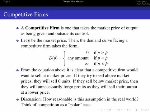
A Competitive Firm is one that takes the market price of outputas being given and outside its control.

Let p be the market price. Then, the demand curve facing acompetitive firm takes the form,

D(p) =

0 if p > p

any amount if p = p∞ if p < p

From the equation above it is clear that a competitive firm wouldwant to sell at market prices. If they try to sell above marketprices, they will sell 0 units. If they sell below market price, thenthey will unnecessarily forgo profits as they will sell their outputat a lower price.

Discussion: How reasonable is this assumption in the real world?Think of competition as a “polar” case.


The Profit Maximization Problem

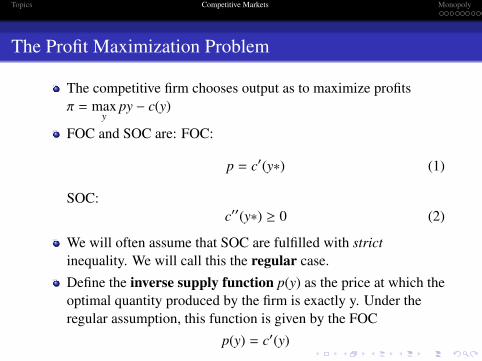
The competitive firm chooses output as to maximize profitsπ = max

ypy − c(y)

FOC and SOC are: FOC:

p = c′(y∗) (1)

SOC:c′′(y∗) ≥ 0 (2)

We will often assume that SOC are fulfilled with strictinequality. We will call this the regular case.Define the inverse supply function p(y) as the price at which theoptimal quantity produced by the firm is exactly y. Under theregular assumption, this function is given by the FOC

p(y) = c′(y)


The Supply Function and Comparative Statics

Define the supply function as the profit-maximizing output ateach price.

p ≡ c′(y(p)) (3)

How does the output of the firm changes with prices? Wedifferentiate (3) with respect to p

1 ≡ c′′(y(p))y′(p) =⇒ y′(p) =1

c′′(y(p))> 0 (4)

We focused on the interior solution. Note that if we assume fixedcosts (F), then it becomes apparent that firms would choose toproduce so long as the lose less than F, the amount they will loseif they chose not to produce at all.

π(y(p)) ≥ −F = py(p) − cυ(y(p)) − F ≥ −F =⇒ p ≥ cυ(y(p))y(p)


The Industry Supply Function

The industry supply function is the sum of the individual firmsupply functions. If there are m firm in the industry, the supplyfunction is,

Y(p) =

m∑i=1

yi(p).

In analogy to the individual firm case, the industry inversesupply function is just the inverse of this function.Example: Different cost functions. Assume two firms, c1(y) = y2

and c2(y) = 2y2. FOC imply that p = c′(y) so that p = 2y1(p) andp = 4y2(p). The industry demand function is justY(p) =

∑i yi(p) = p/2 + p/4 = 3/4p⇒ IISF : p = 4

3 YExample: Identical cost functions. m firms with cost functionc(y) = y2 + 1. FOC yield yi(p) = p/2. The industry supplyfunction isY(p) =

∑mi=1 yi(p) =

∑mi=1 p/2 = mp/2⇒ IISF : p = 2

m Y


Market Equilibrium

An equilibrium price is a price where the amount demandedequals the amount supplied. Why do we call it “equilibrium”? Ifsupply and demand are not equal, then some agents haveincentives to change their behavior. e.g. excess demand woulddrive some consumers out of the market while driving producersinto the market.

Let xi with i = 1, 2, ..., n denote the demand function of each ofthe n consumers and yj denote the supply function of each of them firms. An equilibrium price fulfills the following equation,

n∑i=1

xi(p) =

m∑j=1

yj(p) (5)


Market Equilibrium: An example

Assume the aggregate demand function is X(p) = a − bp and them firms have identical cost function c(yj) = y2

j + 1. We haveshown that the industry supply function is Y(p) = mp/2. (5)implies that in equilibrium X(p) = Y(p). Thus

a − bp =mp2⇒ p∗ =

2am + 2b

In this example, as the number of firms grows, the inverse supplyfunction becomes flatter and the equilibrium price is reduced.Does this property generalize?Consider a generic demand function X(p) and m identical y(p).Then (5) implies, X(p) = my(p). Treat m as an implicit functionof p, X(p(m)) ≡ my(p(m)). We can differentiate this equation:

X′(p)p′(m) = y(p) + my′(p)p′(m)⇒ p′(m) =y(p)

X′(p) − my′(p)< 0


Market Equilibrium: An example

So, in general, with identical cost functions. If the supplyfunction is positively sloped, then the equilibrium price shouldgo down as m increases.

In the previous calculations we assumed m is fixed. However, itwould be reasonable to endogeneize the number of firms. Thistakes us to the entry and exit models. There could be differentmodels depending on the assumption on entry and exit costs.

Assume 0 entry/exit cost and perfect foresight. Let define thebreak-even price p* as the price for which the supply functionyields 0 profits: py(p) − c(y) = 0 and p = c′(y) impliesc′(y) = c(y)/y.


Entry

We have seen that if there are many firms in an industry, thesupply function will be very flat. This, together with thebreak-even condition suggests that the supply curve of acompetitive industry with free entry is simply a flat line thattouches the minimum average cost.

The equilibrium price could be larger than the break-even price ifentry is inhibited by potential entrants perceive that theirentrance would yield negative profits.

Recall that “economic profits” are rents. In this case, this wouldbe a rent for being first in a given market.


Welfare Analysis: Representative Consumer

In this section we investigate the welfare implications ofequilibrium. We will use the representative consumerapproach.

Let’s assume that the market demand curve x(p) is generated bymaximizing utility of a single representative consumer who hasutility u(x, y) = u(x) + y, where x is the good we are interested instudying and y is a kind of aggregate good, often assumed to bemoney.

We have seen that these preferences (quasilinear) produces FOCu′(x(p)) = p, from which the demand curve can be obtained.Recall that this demand curve is independent from income. Thisis useful as simplifies greatly welfare analysis (EV=CS=CV)


Welfare Analysis: Representative Firm and Equilibrium

Now, let’s focus on the other side of the market. We can assumea representative firm with cost function c(x), interpreted as thecost of producing x units of the first good are c(x) units of goody. We assume c(0) = 0, c′(x) > 0 and c′′(x) > 0. This will ensurethat we have a unique solution to the firm’s problem. In thispoint p = c′(x)

Market equilibrium occurs when p = c′(x) = u′(x). This meansthat the marginal utility (marginal willingness to pay) of thegood must be equal to the cost of producing it at the equilibrium.


Welfare Maximization Problem

Imagine that we do not have a competitive market. We just havea consumer that has the quasilinear utility described earlier andaccess to the same technology. Let’s call his problem the“Welfare Maximization Problem”

WMP: maxx,y

u(x) + y subject to c(x) + y = ω. ω is to be interpreted

as the original endowment of good y. Replacing,max

xu(x) + ω − c(x)

FOC ⇒ u′(x) = c′(x) which is the same condition than when weset up a competitive market. In particular, under thisarrangement the quantities produced and consumed of x aregoing to be the same!


Graphical Interpretation

Let define the consumer’s surplus in this context as thedifference between the utility achieved by some output levelminus the cost of the goods. In this case, CS(x) = u(x) − px.Similarly, define producer’s surplus at production level x as thetotal receipts for producing x minus the cost of production.PS(x) = px − c(x)It is evident that the welfare maximization problem could berewritten as:

maxx

u(x)+ω−c(x) = maxx

CS(x)+PS(x)+ω = maxx

CS(x)+PS(x)

where the last equality follows from the fact that ω is a constant.So, a competitive market yields the same solution than directlymaximizing welfare. In particular, these problems are equivalentto maximizing total surplus, TS=CS+PS


Several Consumers and Firms

So far we considered the case of a single consumer and firm.This is easily extended to the case of many consumers indexedby i, i = 1, 2, ..., n and firms indexed by j with j = 1, 2, ...,m

Each consumer has a quasilinear utility functionUi(xi, yi) = ui(xi) + yi and an initial endowment equal to ωi (asbefore, this is measured in terms of the y-good). Each firm facesa cost function that tells them the cost of producing zj units of thex-good is c(zj)

Now the candidate for welfare maximum is the combination thatmaximizes the combined utility of the n consumers that isfeasible, i.e. the j-firms can jointly produce that output level.More formally,



max{xi,yi}

n∑i=1

ui(xi) +

n∑i=1

yi

subject ton∑

i=1

yi =

n∑i=1

ωi −

m∑j=1

cj(zj)

andn∑

i=1

xi =

m∑j=1

zj

The third condition is the new one: it simply says that at theoptimum firms have to choose to produce in aggregate exactlyhow much consumers choose to consume. Putting 1 restrictioninto the objective function, the problem becomes...



max{xi,zj}

n∑i=1

ui(xi) +

n∑i=1

ωi −

m∑j=1

cj(zj)

subject ton∑

i=1

xi =

m∑j=1

zj

let λ denote the lagrange multiplier, then FOC imply

xi : u′i(x∗i ) − λ = 0

zj : − c′j(z∗j ) + λ = 0

λ :n∑

i=1

x∗i =

m∑j=1

z∗j



Again, in this case we have a similar condition that will apply ifwe had an optimum price p∗ = λ. So, the market equilibriummaximizes welfare, at least to the extent that can be measured bythe sum of utilities of individuals!

Related to that point, total utility will typically depend on thedistribution of the initial endowment ωi. In the case ofquasilinear utilities, total utility is independent of the distributionon endowments and any pattern of ωi is consistent withequilibrium.


Pareto Efficiency

A competitive equilibrium maximizes the sum of utilities. It isnot obvious why this should be the relevant objective function tomaximize.

A more general objective would be that it is not possible toimprove one agent’s welfare without reducing the welfare ofsomebody else. This is the idea of Pareto efficiency. If I canmake at least at least one agent better off, without reducing thewelfare of the rest, then there is still room for improvement.

When I reach a point in which I cannot improve anybody withoutharming the rest, then I am at a Pareto efficient point. Note that“pareto efficiency” is relatively free of moral judgements. Forinstance, if people have positive marginal utilities, then acombination in which one agent has everything and the rest hasnothing will be a pareto efficient point!


Pareto Efficiency

Imagine that you have 2 agents in the economy. The totalavailability of good x and y in the economy is (x, y). We wouldlike to find the possible bundles that would maximize the utilityof 1 subject to the constraint that agent 2 gets at least as muchutility as before (u).

maxx1,y1

u1(x1) + y1 (6)

subject to

u2(x − x1) + y − y1 = u (7)

FOC⇒ u′1(x∗1) = u′2(x − x∗1) = u′2(x∗2)

So Pareto efficiency requires that the marginal utility of theconsumption is equalized across consumers.


Pareto Efficiency

Note that the competitive equilibrium satisfies the necessarycondition for pareto efficiency (equalized marginal utilities):p∗ = u′1(x∗1) = u′2(x∗2)

It turns out that this result holds in general (we will study thewelfare theorems later) and not only in the case of quasilinearpreferences.


Pareto Efficiency and Welfare

It may seem puzzle that the same x∗1, x∗2 solve both the welfare

and pareto optimality problems. Let’s have a further look on that.Consider the 2 agent case as before with endowments (x, y)

The “welfare maximization problem looks like:

maxx1,y1,x2,y2

u1(x1) + y1 + u2(x2) + y2 subject to x1 + x2 = x; y1 + y2 = y

which can be simplified to

maxx1,y1

u1(x1) +��y1 + u2(x − x1) + y −��y1

The “pareto efficiency” problem instead is framed as

maxx1,y1

u1(x1) + y1 subject to u2(x − x1) + y − y1 = u

which is simplified to

maxx1,y1

u1(x1) + y1 + u2(x − x1) + y − u


Pareto Efficiency and Welfare

The two problems look identical except for the fact that y1vanishes in the welfare problem but not in the pareto optimalityproblem

This simply means that while any y1 would be consistent with thewelfare equilibrium, only the y1 such that the utility of 2 remainsfixed at u will be consistent in the pareto optimality problem.

Summarizing, while any (y1, y2) would solve the first problem,only one specific y1 would solve the second problem. A specialfeature of quasilinear utility generates this. Under QL utility,x∗1, x

∗2 is determined independently of income (y1, y2). So the set

of all pareto optima allocations is simply (x∗1, x∗2, y1, y2) where

y1 + y2 = y. (interior solution of QL preferences is assumed).


Taxes and Subsidies

A natural change in economic environment is caused by taxesand subsidies. They motivate the idea of comparative statics ineconomics.

A tax will generate a wedge between the price consumers pay forthe good (demand price pd) and the price producers receive fortheir output (supply price, ps).

Let us consider a quantity tax, that is, a tax levied on theamount of a good consumed. If there is a tax of t per each unit ofthe good consumed, then the pd = ps + t.

Alternatively, a value tax is a tax levied on the expenditure in agiven good. If the rate at which expenditure is taxes is τ, thenpd = (1 + τ)ps. This is the case of the VAT.

Subsidies are simple “negative taxes”


Taxes and Subsidies

How does equilibrium change in the presence of subsidies ortaxes?

In the case of the unit tax, the familiar demand equal supplyequation D(p) = S(p) still hold but we have to acknowledge thatdemand reacts to the demand price while supply depends on thesupply price.Solving, D(pd) = S(pd − t) or D(ps + t) = S(ps).

In the case of value taxes the same concept is equal, but therelation between the prices is slightly different. In that caseD(pd) = S(pd/(1 + τ)) or D(ps(1 + τ)) = S(ps) would yield theresult.

Deadweight loss Since taxing will typically increase prices forconsumers and decrease it for producers, it is related to lowerproduction and consumption. The loss in welfare due to theintroduction of the tax is called deadweight loss.


Outline

1 Topics

2 Competitive Markets

3 MonopolyMonopolist ProblemComparative Statics and WelfareQuality choicesPrice discrimination

First-degree price discriminationSecond-degree price discriminationThird-degree price discrimination


Monopolist Problem

Set up

Monopoly: Situation in which one firm is the only seller in onemarket. Note that the definitions is sensitive to how we measurea “market”. Man firms participate in the demand for beverages,but only one in the demand for the mineral water branded“Evian”. If a firm has a demand defined over the good it sells(e.g. consumers are not indifferent to the brand of the mineralwater), then “Evian” can behave as a monopolist in her market,setting up prices or production levels.Under competitions, firms were price-takers. Under monopoly,firms would be price-makersThe monopolist faces 2 constraints:

1 Technological: Just as before there is a technology to transforminputs into output. We will summarize this in the cost functionc(y)

2 Market: Consumers’ demand is a function of how much I wantto charge for my output (this problem did not exist before).


Monopolist Problem

Set up

The monopolist profit maximization problem is:

maxp,y

py − c(y) s.t. D(p) ≥ y

Typically, the consumer will want to produce exactly the amountof goods that he is selling. In that case D(p) = y and the problemsimplifies to:

maxp

pD(p) − c(D(p))

In general, it will be more useful for us to present the problem asone of choosing quantities. Using the inverse demand functionp(y) = D−1(y). Then,

maxy

p(y)y − c(y)

The first and second order conditions for maximization requirethat:


Monopolist Problem

FOC and SOC

p(y) + p′(y)y − c′(y) = 0 (8)

p′(y) + p′′(y)y + p′(y) − c′′(y) = 2p′(y) + p′′(y)y − c′′(y) ≤ 0 (9)

The first condition is the familiar “Marginal Revenue=MarginalCost” condition. Let define r(y) = p(y)y as the revenue of thefirm. Clearly, equation (8) is just r′(y) = c′(y).Economic intuition for the change in revenue:

1 Direct Effect: If he increases his sales by a small quantity dy hemakes an additional pdy.

2 Indirect Effect: In order to increase his sales he has to reduceprices slightly over all units. That is, let dp/dy be the change inprices necessary to sell dy units more, now the indirect effectamounts to y(dp/dy)dy. Since dp/dy < 0, this goes against thedirect effect. Note that IE + DE = pdy + ydp = dr(y)


Monopolist Problem

Elasticity condition

Note that,r′(y) =

dp(y)dy y + p(y) = p(y)[ dp(y)

dyy

p(y) + 1] = p(y)[1 − 1ε(y) ]

where ε(y) is just the price-elasticity of demand, i.e. the percentvariation in demand due to a one percent in prices.

ε(y) = −dy/y

dp(y)/p(y) =dy

dp(y)p(y)

yNote that the monopolist would never operate at a point in whichε < 1.

1 Economic argument: If ε < 1, and I increase prices by 1 percentmy demand decreases ε percent. Since ε < 1, my overall revenuegoes up and my total costs go down (I am producing less!).Hence, profits increase which is inconsistent with maximizingbehavior in the first place. It is easy to see that revenue increases.q1 = q0(1 − (ε/100)) and p1 = p0(1.01), then p1q1 =

(1 + 0.01)(1 − (ε/100))p0q0 ≈ (1 + 0.01 − (ε/100))p0q0 > p0q0.2 Mathematical argument. If ε < 1 then r′(y) < 0 and since

c′(y) > 0, FOC cannot be fulfilled.


Monopolist Problem

Graphical Example

Note that FOC imply r′(y) = c′(y). SOC, in turn, require thatr′′(y) + c′′(y) ≤ 0. That is, that the point where r′(y) = c′(y) theslope of r′(y) is smaller than the slope of c′(y). In other words, itrequires that r′(y) crosses c′(y) from above.

Note also that r′(y) = p(y) + p′(y)y. Since demands are usuallynegatively sloped, then r′(y) < p(y), the marginal revenuefunction lies below the demand function.

Graph †

Linear Case: Assume p(y) = a − by and c(y) = cy. Then y∗ = a−c2b

and p∗ = a+c2 . †

Constant Elasticity Demand: p∗ = c1− 1

ε

, i.e. the optimal price is

just a constant markup over cost. †


Comparative Statics and Welfare

Comparative Statics

Assume for simplicity that marginal cost is fixed at c. So thatc(y) = cy

Define y(c) as the optimal response to changes in marginal cost.Then p′(y(c))y + p(y(c)) ≡ c

The implicit function theorem yields: y′(c) = 1p′′(y(c))y(c)+2p′(y(c))

The chain rule implies that: dpdc =

dpdy

dydc =

p′(y(c))p′′(y(c))y(c)+2p′(y(c))

Simplifying: dpdc = 1

p′′(y(c))y(c)p′(y(c)) +2

Linear function⇒ dpdc = 1

2 . Constant elasticity of demand⇒dpdc = ε

ε−1 .1

Note that in the case of constant elasticity, the price increasesmore than proportionally when cost increase!

1In the book some formulas differ. This is because ε = −εVarian



Welfare Considerations

We have seen that if markets are competitive p = c′(y) yields aquantity that is Pareto efficient.

We have seen that r(y) is always below the inverse demand p(y),so that monopoly must produce lower quantities (look at thegraph). However, how severe is this inefficiency is yet to bestudied.

Assume a 1-consumer economy with quasilinear utility u(x) + y.This yields a nice inverse utility function p(x) = u′(x). Let c(x)denote the cost (in terms of y) of producing x units of thex-good. A welfare function is the one that maximizes utilityy = m − c(x) and m is fixed, this is like maximizing

W(x) = u(x) − c(x)




At the social optimum, FOC require that u′(xso) = c′(xso). As wesaw, monopoly satisfies the relation, p′(xm)xm + p(xm) = c′(xm).Use the fact that p(x) = u′(x), then this condition implies that

u′′(xm)xm + u′(xm) = c′(xm) (10)

The derivative of the social welfare function evaluated at themonopoly equilibrium xm is

W′(xm) = u′(xm) − c′(xm) = −u′′(xm)xm > 0 (11)

where I have used (10) and the fact that u(.) is a concavefunction.This means that at the monopolist quantities, we can stillimprove welfare as there are people willing to pay more thanwhat it costs to produce one more unit of x. Graph †


Quality choices


So far, we assumed that the only dimension of the monopolistchoice were quantities. What if the monopoly could decide overthe quality of the good produced? Let q denote the units of“quality”. It is reasonable to assume that ∂u(x, q)/∂q > 0 and∂c(x, q)/∂q > 0. That is, consumers value quality and quality iscostly.

The monopolist maximization problem is now:max

x,qp(x, q)x − c(x, q).

FOC for this problem are:

p(xm, qm) +∂p(xm, qm)

∂xxm =

∂c(xm, qm)∂x

(12)

∂p(xm, qm)∂q

xm =∂c(xm, qm)

∂q(13)


Quality choices


Adding quality to the welfare function we saw beforeW(x, q) = u(x, q) = c(x, q). The first order conditions evaluated,not at the optimum, but at the monopolist equilibrium yield:

∂W(xm, qm)∂x

=∂u(xm, qm)

∂x−∂c(xm, qm)

∂x= −

∂p(xm, qm)∂x

xm > 0

where I have used the fact that preferences are quasilinear andequation (12) to get the second equality.

Similarly, you can use FOC for the amount of quality andequation (13) to get:

∂W(xm, qm)∂q

=∂u(xm, qm)

∂q−∂c(xm, qm)

∂q=∂u(xm, qm)

∂q−∂p(xm, qm)

∂qxm


Quality choices


As it was before, the first equation says that keeping qualityfixed, an increase in quantity will increase social welfare.

The effect of an increase of quality on welfare are, however,ambiguous. Clearly, the second part (the marginal cost) ispositive and so is the first part (marginal utility). At themonopolist quantities, it is not clear whether the wholeexpression will be positive or negative!

Rearraging the second equation:1

xm

∂W(xm,qm)∂q = ∂

∂q [ u(xm,qm)xm

− p(xm, qm)]

The derivative of the welfare with respect to quality isproportional to the derivative of the average willingness to payminus the marginal willingness to pay. Unless that these two areequalized at the monopolist solution (xm), this will fail toproduce the optimal quantity of “quality”.


Price discrimination

Idea

Price discrimination occurs when a monopolist can sell differentunits of the same good at different prices, either to the same ordifferent consumers.

Recall that the main problem why the monopolist sold too fewunits is because in order to sell an extra unit, it had to reduce theprice of all the previously sold units. If the monopolist finds away to sell at different prices the same good, then he will sellmore units.

A key issue is that the markets should be fragmented, in thesense, that if there are two prices but people can sell and buybetween them, then everybody would have an incentive toarbitrage, i.e. buy in the market that sells cheap and sell it in themarket that buys at the expensive price.



Idea

The easy way to discriminate is to do it with respect to somecategory that is endogenous to consumers, i.e. age.

If the discrimination is done over a choice variable for theconsumer (quantities consumed, time of the purchase) them themonopolist has to structure his pricing in such a way that theconsumers will sort themselves out in the right category.There are three types of price-discrimination

1 First-degree price discrimination/perfect price discrimination:The monopolist can charge to each consumer exactly a priceequal to her willingness to pay for that unit.

2 Second-degree price discrimination: When prices differaccording to the number of units bought but not on the consumer.e.g. quantity discounts.

3 Third-degree price discrimination: Different consumers getcharged different prices.



First-degree price discrimination

Imagine that the monopolist faces only one agent. He gets tooffer a “take-it-or-leave-it” combination of output and (overall)price (r∗, x∗). Assuming linear costs as before, his profitmaximization problem would be:

maxr,x

r − cx s.t. u(x) ≥ r

where the constraint just says that the consumer should bewilling to accept the deal, so he should get at least enough utilityfrom consuming the good than what he pays for it.

FOC for this problem, noting that the monopolist would neverchoose r∗ < u(x), is:

u′(x∗) = c⇒ r∗ = u(x∗) (14)



Features of FDPD

There are a few interesting characteristics of this solution:1 The amount produced coincides with the amount produced under

competition (see (14)). The monopolist chooses a Paretooptimum quantity.

2 However, in sharp contrast with the competitive solution, themonopolist gets all the surplus (both the consumers and theproducers)!

3 The reason for this is that the consumer can sell now additionalunits without lowering the price of the units he had “previously”sold.



Example

Assume that the monopolist can break up its production inn-pieces (x = n∆x) and, crucially, that he can charge a differentprice for each fraction pi, where i stands for the order in whichthe fraction is sold. As usual, assume quasilinear preferences onthe consumer.Then he would charge a price so that the consumer is justindifferent between buying it or not. For the first ∆x units in themarket we will equalize

u(0) + m︸︷︷︸He doesnt consume the good

= u(∆x) + m − p1︸︷︷︸He consumes the first ∆ units

⇒ u(0) = u(∆x) − p1

Similarly for the second fraction, the consumer would already beconsuming ∆x, so the monopolist would equalize:

u(∆x) +�m −��p1 = u(2∆x) +�m −��p1 − p2 (15)



Example (cont.)

You can continue up until the last unit of the good.

u((n − 1)∆x) = u(n∆x) − pn (16)

Summing up all these n equations we get:n∑

i=1

u((i − 1)∆x) =

n∑i=1

u(i∆x) −n∑

i=1

pi (17)

Canceling out all the intermediate terms in the sum of u(.)’s,

u(0) = u(n∆x) −n∑

i=1

pi (18)

Normalizing u(0) = 1 and using the fact that x = n∆x,

u(x) =

n∑i=1

pi (19)



Example (cont.)

What equation (19) says is that the sum of the marginalwillingness-to-pay should equal the aggregate willingness to payfor that amount of x.

So as long as the firm can charge a different price each differentunit of the same good, she would be producing at a point inwhich everybody who is willing to pay more than what the goodcosts, would get the good. It is not crucial the assumption of atake-it-or-leave-it offer we did before!



Second-degree price discrimination

This is non-linear prices. That is, charging different pricesaccording to the quantities bought (e.g. quantity discounts).

Assume there are 2 consumers with utility functions u1(x1) + y1and u2(x2) + y2, where u2(x) > u1(x) and u′2(x) > u′1(x). We willcall 2 the High-demand consumer and 1 the low-demandconsumer.

The property that the agent with the largest utility (and averageutility) of x, also has the largest marginal utility at x is calledsingle crossing property. This condition implies that theindifference curves can cross at most once.

Now the monopolist gets to choose a function ri = p(xi)xi thatshows how prices change with xi



Idea

The monopolist has 2 set of restrictions. First, consumers shouldfind it convenient to purchase the good

u1(x1) − r1 ≥ 0

u2(x2) − r2 ≥ 0

Second, each consumer has to self-select himself into the groupthat maximizes monopolist income

u1(x1) − r1 ≥ u1(x2) − r2

u2(x2) − r2 ≥ u2(x1) − r1



Idea

These equations imply the following restrictions. In general,only one of each restrictions will be binding as the monopolistwants to maximize r1 and r2.

r1 ≤ u1(x1) (20)

r1 ≤ u1(x1) − u1(x2) + r2 (21)

r2 ≤ u2(x2) (22)

r2 ≤ u2(x2) − u2(x1) + r1 (23)

It turns out that with the single crossing property it is enough toknow which inequality will be binding.



Idea

Assume (22) is binding. Then r2 = u2(x2), ((23))⇒ u2(x1) ≤ r1.But this last inequality leads to a contradiction.u1(x1) < u2(x1) ≤ r1 ≤ u1(x1). Where the first inequality comesfrom single crossing and the third comes from (20). Then (23)should be binding.Let’s turn to the other set of restrictions. Assume (21) is binding.Then r1 = u1(x1) − u1(x2) + r2. Substitute r2 from (23) that wenow know is binding. Then,��r1 = u1(x1) − u1(x2) + u2(x2) − u2(x1) +��r1This last equality means that

x2∫x1

u′1(x)dx =

x2∫x1

u′2(x)dx (24)

But this contradicts the single crossing property: u′2(x) > u′1(x).Then (20) is binding.



Idea

Putting these two results together we get that r1 = u1(x1) so thatthe low demand consumer is charged his willingness to pay.Also, r2 = u2(x2) − u2(x1) + r1, so the high demand agent ischarged the maximum amount possible provided that he wouldstill consume x2.

The profits of the consumer are given byπ = [r1−cx1]+[r2−cx2] = u(x1)−c(x1)+u2(x2)−u2(x1)+u(x1)−cx2where we have used the two conditions from above.

FOC yield:

u′1(x1) − c + u′1(x1) − u′2(x1) = 0 (25)

u′2(x2) − c = 0 (26)



Idea

(25) can be rearranged to show that:

u′1(x1) = [u′2(x1) − u′1(x1)] + c > c (27)

where the last inequality follows from single crossing (i.e.u′2(x) > u′1(x) for all x).From (26) and (27) there are 2 outstanding facts. Undernon-linear prices, the consumer with “low demand” consumestoo few units and too expensive (the monopolist fixes thequantities/price at a point in which the marginal willingness topay exceeds the cost of producing it. Recall, at a socially optimalconsumption bundle, the marginal willingness to pay has to beequal to marginal cost.The high demand consumer would consume exactly as manyunits as socially efficient (that is, marginal willingness to payequals the marginal cost).



Final thoughts

In general, we will always expect the high-demand to consumethe right quantity. This is so because if the high type wereconsuming less, the monopolist could reduce the price he’sfacing and (since price is above marginal cost) still make a profit.Unlike the non-discrimination case, the change in price wouldonly affect the high type and not the rest of the buyers!



Third-degree price discrimination

In this case, prices are the same for consumers in the same group,but vary across different groups of consumers. Very commonsituation: discounts for the elderly, discount for the young etc.In this case, the separation between the two groups is verysimple. Assume the cost of the units is the same regardless of thegroup the monopolist is selling to. Let pi(xi) denote the inversedemand function. Then the monopolist is seeking to maximizep1(x1)x1 + p2(x2)x2 − cx1 − cx2.FOC in this case are,

p′i(xi)xi + pi(xi) = c

Which leads to a elasticity condition (see above),

pi(xi)[1 −1εi

] = c



This conditions them mean,

p′1(x1)[1 −1ε1

] = p′2(x2)[1 −1ε2

]

That is if ε1 < ε2 then p1 > p2. Is it intuitive?

Think about it, you are charging more to the group the the mostinelastic demand. Since they are not so responsive to prices, youcan charge them more. The group with elastic demands, wouldreduce significatively their demand when you increase the price.

Think about next time you get a student discount!



In the previous discussion we assumed the monopolist couldseparate markets perfectly. What if that’s not the case? “Dia delespectador”. In practical terms this means that pi(x1, x2). Themonopolist problem is now,

maxx1,x2

p1(x1, x2)x1 + p2(x2, x2)x2 − cx1 − cx2

The first order conditions now can be written as

pi + ∂pi(x1, x2)/∂x1 + ∂pi(x1, x2)/∂x2 = c

In terms of elasticity the condition becomes now

p1[1 −1ε1

] + ∂p2/∂x1x2 = c

p2[1 −1ε2

] + ∂p1/∂x2x1 = c



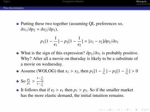
Putting these two together (assuming QL preferences so,∂x1/∂p2 = ∂x2/∂p1),

p1[1 −1ε1

] − p2[1 −1ε2

] = [x1 − x2]∂p2/∂x1

What is the sign of this expression? ∂p2/∂x1 is probably positive.Why? After all a movie on thursday is likely to be a substitute ofa movie on wednesday.

Assume (WOLOG) that x1 > x2, then p1[1 − 1ε1

] − p2[1 − 1ε2

] > 0

So p1p2>

1− 1ε2

1− 1ε1

It follows that if ε2 > ε1 then p1 > p2. So if the smaller markethas the more elastic demand, the initial intuition remains.



Welfare considerations of third-order price discrimination

Idea: Are consumers better off if the monopolist can use pricediscrimination?Under quite general conditions 2 the necessary and sufficientconditions for welfare improvement are:

Necessary condition: The total quantities sold increase whenprice discrimination is allowed.Sufficient condition: The weighted sum of quantities are positive.Where each quantity is weighted by the difference between priceand marginal cost. Imagine this set up: MC = 5, p1 = 16, p2 = 9,∆x1 = −4 and ∆x2 = 10. The initial price was 10. The totalquantity increased ∆x1 + ∆x2 = 6 but the weighted quantity is(16 − 5)(−4) + (9 − 5)(10) = −4. In this case, welfare decreases.

Some special cases: (1) Linear demand implies that no change inoverall quantities. It is not welfare increasing; (2) Ifdiscrimination opens new markets (Ryanair!) then it is welfareincreasing.

2Quasilinear utility function with u(.) strictly concave, constant marginal cost

Documents

Market Structure: Competition vs. Monopoly Structure: Competition vs. Monopoly Juan Manuel Puerta November 9, 2009. TopicsCompetitive Markets Monopoly ... equilibrium quantities and