Markov Chains with Memory, Tensor Formulation, and the Dynamics ofPower Iteration

Sheng-Jhih Wua, Moody T. Chub,1

aCenter for Advanced Statistics and Econometrics Research,School of Mathematical Sciences, Soochow University, Suzhou, China.bDepartment of Mathematics, North Carolina State University, Raleigh, NC 27695-8205.

Abstract

A Markov chain with memory is no different from the conventional Markov chain on the product state space.Such a Markovianization, however, increases the dimensionality exponentially. Instead, Markov chain withmemory can naturally be represented as a tensor, whence the transitions of the state distribution and the mem-ory distribution can be characterized by specially defined tensor products. In this context, the progression ofa Markov chain can be interpreted as variants of power-like iterations moving toward the limiting probabilitydistributions. What is not clear is the makeup of the “seconddominant eigenvalue” that affects the conver-gence rate of the iteration, if the method converges at all. Casting the power method as a fixed-point iteration,this paper examines the local behavior of the nonlinear map and identifies the cause of convergence or di-vergence. As an application, it is found that there exists anopen set of irreducible and aperiodic transitionprobability tensors where theZ-eigenvector type of power iterates fail to converge.

Keywords: Markov chain with memory, transition probability tensor, stationary distribution, power method,rate of convergence, second dominant eigenvalue2000 MSC:15A18, 15A51, 15A69, 60J99

1. Introduction

A Markov chain is a stochastic processXt∞t=0 over a finite state spaceS, where the conditional prob-ability distribution of future states in the process depends upon the present or past states. The classical“Markov property” specifies that the probability of transition to the next state depends only on the probabilityof the current state. That is, among the statessi ∈ S, the model assumes that

Pr(Xt+1 = st+1|Xt = st, . . . , X2 = s2, X1 = s1) = Pr(Xt+1 = s|Xt = st).

For simplicity, identify the states asS = 1, 2, . . . , n and assume that the chain is time homogeneous. Thena transition probability matrixP = [pij ] defined by

pij := Pr(Xt+1 = i | Xt = j) (1)

is independent oft and column stochastic. The above process is, generally characterized as memoryless2, isa well studied subject.

There are situations where the data sequence does depend on past values. As can be expected, the addi-tional history of memory often has the advantage of offeringa more precise predictive value. By bringingmore memory into the random process, we can build a higher order Markov model. Interesting applications

Email addresses:szwu@suda.edu.cn (Sheng-Jhih Wu),chu@math.ncsu.edu (Moody T. Chu)1This research was supported in part by the National Science Foundation under grant DMS-1316779.2Strictly speaking, it should be called a chain with memory 1 based on the definition (2).

Preprint submitted to Elsevier August 4, 2016

include packet video traffic in larger buffers [25], finance risk management [17, 18, 27], wind turbine design[24], alignment of DNA sequences or long-range correlated dynamic systems [19, 20, 28], growth of polymerchains [6, 12], cloud data mining [9, 26], and many others [16]. A Markov chain with memorym is a processsatisfying

Pr(Xt+1 = st+1|Xt = st, . . . , X1 = s1) = Pr(Xt+1 = st+1|Xt = st, . . . , Xt−m+1 = st−m+1) (2)

for all t ≥ m. By definingYt = (Xt, Xt−1, ..., Xt−m+1) (3)

and by taking the orderedm-tuples ofX values as its product state space, it is easy to see that the chainYt with suitable starting values satisfies the Markov property. In principle, upon exploiting the underlyingstructure, the transition process can be analyzed with the classical theory for memoryless Markov chain. Note,however, that the size of the aggregated chain, also known asthe Markovianization, is considerably larger —of dimensionnm−1. Though mathematically equivalent, basic tasks such as bookkeeping multi-states andother associated operations will be fairly tedious3.

In recent years higher-order tensor analysis have become aneffective way to address high-throughputand multi-dimensional data by different disciplines. Markov chain with memory fits naturally such a tensorformulation. Assuming again time homogeneity, a Markov chain with memorym − 1 can be convenientlyrepresented via the order-m tensorP = [pi1i2...im ] defined by

pi1i2...im := Pr(Xt+1 = i1|Xt = i2, . . . , Xt−m+2 = im), (4)

whereP is called a transition probability tensor. Necessarily we have the properties that0 ≤ pi1i2...im ≤ 1and that

n∑

i1=1

pi1i2...im = 1 (5)

for every fixed(m − 1)-tuple(i2, . . . , im). What is most interesting is that the transitions among the statesas well as the history of memory can be characterized by specially defined tensor products. Our goal in thispaper is to recast such a process under the tensor formulation. In particular, we are interested in understandingthe dynamics of the transition to the stationary distribution and the associated 2-phase power iteration schemein the context of tensor operations.

While some classical results in matrix theory can be extended naturally to tensors, there are cases wherethe nonlinearity of tensors makes the generalization far more cumbersome. The notion of eigenvalue isone such incident. Depending on the applications, there areseveral ways to mull over how an eigenvalueof a tensor should be defined [3, 13, 14, 23]. Markov chain withmemory and the associated transitionprobability tensor can serve as a practical model for exploring the following two notions of eigenvalues andtheir implications:

1. The classical concept of eigenvalues when characterizing the evolution of the joint probability massfunctions.

2. The notion ofZ-eigenvalue [23] when approximating the evolution of the state probability distribution.

In this context, we study the role of the “second dominant eigenvalue” in such a dynamics of a Markovchain with memory. We also intend to address some practical issues arisen from a recent discussion in[12] which proposes to short cut the computation of the stationary state distribution by approximating thestationary joint probability mass function. These issues include whether the assumption used in proposingtheZ-eigenvector computation is statistically justifiable andthe anatomy of the true cause that affects the rateof convergence. The tool we are about to develop gives some insight into this limiting behavior. It is possibleto generalize our framework to other types of eigenvalues for tensors, e.g., the so calledH-eigenvalues [21].

3See an example of vectorizing a Markov chain with memory 2 in Section 3.

2

For demonstration, we choose to concentrate only on the application to the transition probability tensors inthis presentation.

This paper is organized as follows. We begin in Section 2 withsome basic properties of transition proba-bility tensors. We review two types of dynamics necessarilyinvolved in a Markov chain with memory, eachof which entails a particular kind of tensor product. The evolution of the joint probability mass functionitself follows a scheme similar to the conventional power method, whereas finding the stationary probabil-ity distributions of the state vector requires a 2-phase iteration. In Sections 3, we argue that an appropriaterearrangement of the transition probability tensor reveals the proper cause of convergence for this classicaltype of evolution. In Section 4 we address some concerns arisen from the recent notion of approximatingthe stationary distribution by the dominantZ-eigenvector. We identify the true makeup of the “second”dominant eigenvalue in the tensor setting. Most importantly, we show that the convergence of this shortcuttype of power method proposed in [12] is not always guaranteed by counter examples. Included in the Ap-pendix is the local analysis in a similar spirit for matrices, which probably offers an alternative explanationof convergence for the classical power method .

2. Dynamics involved in a Markov chain with memory

Needless to say, a critical ingredient in the Markov processwith memorym − 1 is the joint probabilitymass function of state variablesXt, . . . Xt−m+2 overS at timet, denoted as

Πt,t−1,...,t−m+2 = [π(t)i2...im

], (6)

whereπ(t)i2...im

:= Pr(Xt = i2, . . . , Xt−m+2 = im).

Note thatΠt,t−1,...,t−m+2 is an order-(m−1) tensor whose entries are nonnegative and satisfy the identity

n∑

i2,...,im=1

π(t)i2...im

= 1. (7)

With appropriate ordering, the joint probability mass function Πt,t−1,...,t−m+2 is simply the typical statedistribution of the Markovianized(m− 1)-tuple(Xt, . . . , Xt−m+2).

The definition of conditional probability naturally dictates that in a Markov chain with memory the prob-ability distribution of the next stateXt+1 based on memoryXt, . . . Xt−m+2 should be calculated in thefollowing way which naturally defines a kind of tensor product, denoted by the symbol⊛1.

Lemma 2.1. Let the column vectorx(t+1) denote the probability distribution of the variableXt+1 over thestate spaceS. Then

x(t+1) = P ⊛1 Πt,t−1,...,t−m+2 := [〈pi1,:,Πt,t−1,...,t−m+2〉] ∈ R

n, (8)

wherepi1,: denotes thei1-th facet in the1st direction ofP and〈·, ·〉 is the Frobenius inner product generalizedto multi-dimensional arrays.

We claim that entries of the next joint probability mass function Πt+1,t,...,t−m+3 = [π(t+1)i1...im−1

] of statevariablesXt+1, . . .Xt−m+3 are given as follows, which defines another kind of tensor product. Once thiscalculation is complete, it allows the chain to continue evolving.

Lemma 2.2. Given the joint probability mass functionΠt,t−1,...,t−m+2, if Xt+1 is obtained from the Markovchain with memoryXt, . . . Xt−m+2, then the entries ofΠt+1,t,...,t−m+3 are given by

π(t+1)i1...im−1

=

n∑

im=1

pi1i2...imπ(t)i2...im

, i1, . . . , im−1 = 1, . . . , n. (9)

3

Proof. Observe that

Πt+1,t,...,t−m+3 =

n∑

im=1

Pr(Xt+1, Xt, . . . , Xt−m+3, Xt−m+2 = im)

=

n∑

im=1

Pr(Xt+1|Xt, . . . , Xt−m+3, Xt−m+2 = im) Pr(Xt, . . . Xt−m+3, Xt−m+2 = im). (10)

The expression (9) is simply the case whenXt+1 = i1, Xt = i2, . . ., Xi−m+3 = im−1.Note that the operation required in (9) is different from theusual mode-m tensor product defined in the

literature [10]. For convenience, denote this process for transiting the joint probability mass function by thesymbol

Πt+1,t,...,t−m+3 = P Πt,t−1,...,t−m+2. (11)

As an demonstration of this operator, we can rewrite the relation (9) for a Markov chain with memory 2 inthe matrix form as

Πt+1,t = [P(:, 1, :)Πt,t−1(1, :)⊤, . . . ,P(:, n, :)Πt,t−1(n, :)

⊤] (12)

whereP(:, j, :) ∈ Rn×n andΠt,t−1(j, :) stand for thej-th facet in the2nd direction ofP and thej-th rowof Πt,t−1, respectively. The summation over the indexi3 is included in the matrix-to-vector multiplication.In contrast, for a Markov chain with memory 1 (the so called memoryless case), the products⊛1 and areidentical andΠt+1 = x

(t+1).Our understanding thus far is derived from elementary probability theory. It implies that, for a Markov

chain with memory greater than 1, there are two dynamics involved in the evolving process. One is themultiplication in the form of (8) for the transition of statedistribution. The other is the multiplication in theform of (11) for the transition of the joint probability massfunction. To characterize the limiting behavior ofthe state distributionx(t), it is necessary to understand the limiting behavior of the joint probability massfunctionΠt,t−1,...,t−m+2, and vice versa. Although the approach is standard, we find little discussion in theliterature that analyzes these processes directly in the setting of tensors [8]. In the following, we demonstratethat the tensor notation is convenient for arguing the dynamics behavior of Markov chains.

3. Power iteration for joint probability mass function

In this section, we elaborate further on the limiting behavior of the joint probability mass functionΠt,t−1,...,t−m+2. It will be instructive if we first consider the Markov chain with memory 2, which givesrise to an order-3 probability transition tensor. The discussion can readily be extended to the general case.

For a Markov chain with memory 2 to move forward, we have to process two sequences of probabilitydistributions hand by hand. At the time stept, we have a distributionΠt,t−1 = [πi2i3 ] for memory(Xt, Xt−1)overS × S. Then the next stateXt+1 overS based on this memory has a distributionx

(t+1) defined by thetensor product

x(t+1) = P ⊛1 Πt,t−1. (13)

In the meantime, the memory distribution is also evolved into

Πt+1,t = P Πt,t−1. (14)

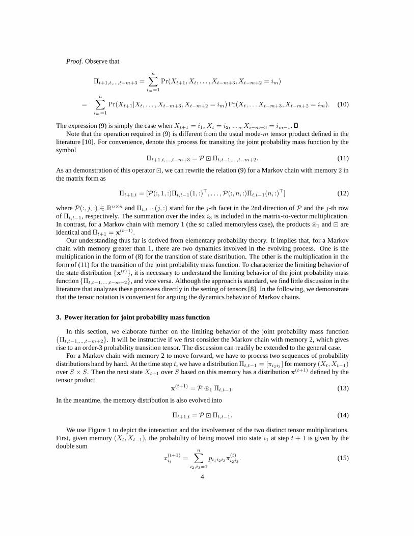
We use Figure 1 to depict the interaction and the involvementof the two distinct tensor multiplications.First, given memory(Xt, Xt−1), the probability of being moved into statei1 at stept + 1 is given by thedouble sum

x(t+1)ii

=

n∑

i2,i3=1

pi1i2i3π(t)i2i3

. (15)

4

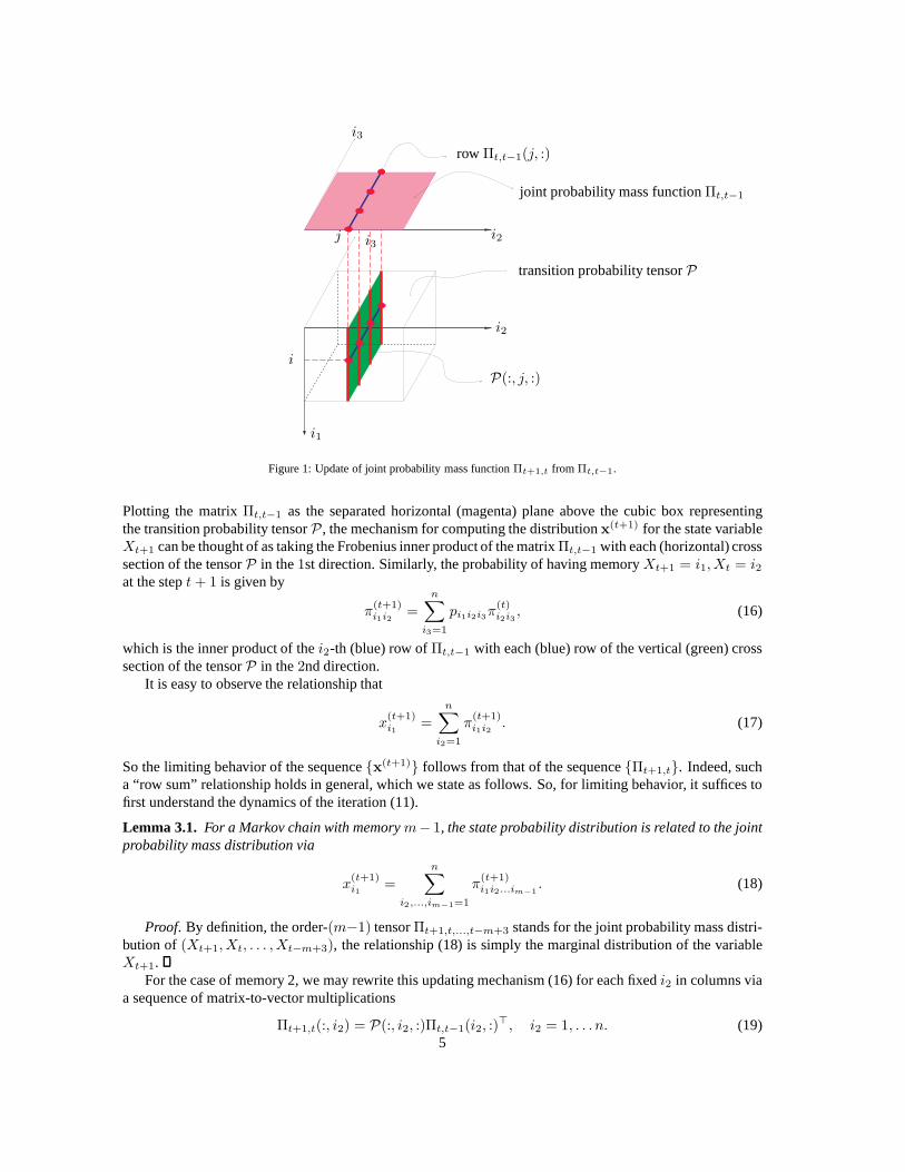
i1

i2

i2

i3

i3

i

j

P(:, j, :)

joint probability mass functionΠt,t−1

transition probability tensorP

rowΠt,t−1(j, :)

Figure 1: Update of joint probability mass functionΠt+1,t fromΠt,t−1.

Plotting the matrixΠt,t−1 as the separated horizontal (magenta) plane above the cubicbox representingthe transition probability tensorP , the mechanism for computing the distributionx

(t+1) for the state variableXt+1 can be thought of as taking the Frobenius inner product of thematrixΠt,t−1 with each (horizontal) crosssection of the tensorP in the1st direction. Similarly, the probability of having memoryXt+1 = i1, Xt = i2at the stept+ 1 is given by

π(t+1)i1i2

=

n∑

i3=1

pi1i2i3π(t)i2i3

, (16)

which is the inner product of thei2-th (blue) row ofΠt,t−1 with each (blue) row of the vertical (green) crosssection of the tensorP in the2nd direction.

It is easy to observe the relationship that

x(t+1)i1

=

n∑

i2=1

π(t+1)i1i2

. (17)

So the limiting behavior of the sequencex(t+1) follows from that of the sequenceΠt+1,t. Indeed, sucha “row sum” relationship holds in general, which we state as follows. So, for limiting behavior, it suffices tofirst understand the dynamics of the iteration (11).

Lemma 3.1. For a Markov chain with memorym− 1, the state probability distribution is related to the jointprobability mass distribution via

x(t+1)i1

=

n∑

i2,...,im−1=1

π(t+1)i1i2...im−1

. (18)

Proof. By definition, the order-(m−1) tensorΠt+1,t,...,t−m+3 stands for the joint probability mass distri-bution of(Xt+1, Xt, . . . , Xt−m+3), the relationship (18) is simply the marginal distributionof the variableXt+1.

For the case of memory 2, we may rewrite this updating mechanism (16) for each fixedi2 in columns viaa sequence of matrix-to-vector multiplications

Πt+1,t(:, i2) = P(:, i2, :)Πt,t−1(i2, :)⊤, i2 = 1, . . . n. (19)

5

At first glance, such a scheme seems to be the familiar power method4 applied to the matrixP(:, i2, :). Thesubtle difference is at the “transpose” involved in (19). Inorder to repeat the “matrix-to-column” multiplica-tion for a fixedi2, we must know every other “rows” ofΠt+1,t which is not available until the entire sequenceof multiplications in the form of (19) has been completed. Inother words, only by treating the operation in(14) as a whole “tensor-to-tensor” multiplication, we may treat the iteration as a power method. This is notan ordinary power iteration.

We certainly can recast the power-like iteration (14) in theusual context of matrix operations as follows.This should manifests the complication of the “second dominant eigenvalue” of the order-3 tensorP . See also[8] for a similar discussion. Letvec(M) denote the conventional vectorization of the matrixM by stackingits columns into a single column vector. LetC be then2 × n2 permutation matrix that does the swapping ofindices

(j − 1)n+ i → (i− 1)n+ j, 1 ≤ i, j ≤ n.

Also, letB denote then2×n2 block diagonal matrix whosei2-th diagonal block is precisely then×n matrixP(:, i2, :). Then the operation is equivalent to the matrix-to-vector multiplication

vec(Πt+1,t) = BCvec(Πt,t−1). (20)

The scheme (20) is exactly the power method applied to then2 × n2 matrixA := BC. It is not difficult tocheck thatA has the block structure

A=

P(:, 1, 1) 0 . . . 0 P(:, 1, 2) 0 . . . 0 . . . P(:, 1, n) 0 . . . 00 P(:, 2, 1) 0 0 P(:, 2, 2) 0 . . . 0 P(:, 2, n) 0

.

.

....

. . ....

.

.

....

. . .... . . .

.

.

....

. . ....

0 0 . . . P(:, n, 1) 0 0 . . . P(:, n, 2) . . . 0 0 . . . P(:, n, n)

,

where eachP(:, i, j) is a column vector inRn. By (5), A is itself column stochastic. By (7),vec(Πt,t−1)is itself a distribution vector. This is one way to “unfold” an order-3 transition probability tensorP into acolumn stochastic matrixA. From this point on, the following results follow from what we already knowabout the conventional power method applied to the matrixA.

Lemma 3.2. Suppose thatP is the transition probability tensor of a Markov chain with memory 2. Assumethat the Perron rootλ1(A) = 1 of the correspondingA is simple. Then, starting with any generic initialmemory distributionΠ0,−1, the following statements hold.

1. The convergence of the joint probability mass functions generated by (14) is guaranteed.2. The limit pointΠ of joint probability mass functions is the de-vectorization of the normalized dominant

eigenvector ofA under the 1-norm.3. The stationary distributionx of the states under this Markov chain (13) with memory 2 exists and is

the row sum ofΠ.4. The rate of convergence is the modulus of the second dominanteigenvalue of the matrixA.

Though we shall not carry out the “unfolding” explicitly, the above argument is generalizable to Markovchains with memory higher than 2. One quick way to look at thissituation is to regard the Markov processof P acting on the joint probability mass function via the multiplication defined by (11) as a linear mapfrom the spaceTm−1 of order-(m− 1) tensors toTm−1 itself. Any finite dimensional linear relationship canalways be expressed in terms of a matrix-to-vector multiplication. Therefore, the convergence of the sequenceΠt,t−1,...,t−m+2 generated by the iteration (11) can be guaranteed. The tedious work is to construct thecorresponding column stochastic matrixA, once we specify how the tensorΠt,t−1,...,t−m+2 is to be flattenedinto a vector. The latter depends on how the multi-dimensional statesXt, . . . , Xt−m+2 are to be ordered.When all the details are done, then the “second dominant eigenvalue” of the resulting matrixA determinesthe rate of convergence.

4For a quick overview of the power method and its convergence,see the Appendix in Section 6.

6

Thus far, we have argued that the Markov evolution for the joint probability mass function naturallyinduces a power-like iteration under the multiplication. The corresponding mapP : Tm−1 → Tm−1 is alinear transformation. In this context, the notion of eigenvalue for the tensorP should be defined in exactlythe same way as we usually do for square matrices, barring thepeculiar operation for multiplication. Suchan approach is not always the one adopted in the literature. For instance, we ponder upon the so calledZ-eigenvector and compare it with the dominant eigenvector under in the next section.

4. Power iteration for Z-eigenvector computation

The relationship (8) characterizes the dynamics of the probability distributionx(t+1) in terms ofΠt,t−1,...,t−m+2

which itself evolves according to (11). This is by far the most formal way to describe the actual evolution ofthe state distribution for a Markov chain with memory. By continuity, the stationary distribution of the statessatisfies the same relationship (8) with the limiting joint probability function of (11). For the latter, we havepostulated its existence through the standard argument forthe power method in the preceding section.

Recently it has been proposed to circumvent the 2-phase evolution process by assuming directly that alimiting joint probability distribution of the high-orderMarkov chain is the Kronecker product of its limitingprobability distribution [12]. The rationale is that if thesequencex(t) has ever reached a stationary distri-butionx overS, then it seems reasonable to assume that the limiting joint probability mass function be of theform

limt→∞

Πt,t−1,...,t−m+2 = x⊗ x⊗ . . .⊗ x︸ ︷︷ ︸m−1 times

. (21)

Under this assumption, it is deduced from (8) that the stationary distributionx should satisfy the equation

P ⊛1 z⊗ z⊗ . . .⊗ z = z (22)

which is conveniently abbreviated asPz

m−1 = z (23)

in the literature. The solution to (23) is called theZ-eigenvector associated with, in this case, the unitZ-eigenvalue ofP [2, 13, 14, 23]. It can be shown that a solution to (23) does exist and that entries of any sucha solution are all positive, ifP is irreducible [12, Theorem 2.2]. Under some additional conditions onP , iteven can be shown that the solution is unique [4, 12].

In addition toZ-eigenvalues, there are other ways to define eigenvalues fora given tensor [13, 14, 23].Accordingly, a variety of methods has been proposed for computing eigenpairs of a tensor [5, 12, 15, 21, 30,31]. Perhaps the simplest means for finding theZ-eigenvectorz in (23) is an iterative scheme5 of the form

zk+1 := Pzm−1k , (24)

where the starting pointz0 is an arbitrary probability vector. Note that eachzk+1 remains to be a probabilityvector under exact arithmetic6. Under some mild conditions, the sequencezk does converge linearly to asolution of (23).

While studying the nonlinear equation (23) and the dynamicsof power-like iteration (24) is of mathemat-ical interest in its own right, we want to point out that thereare serious issues associated with the assumption(21) for Markov chains with memory.

5Thoughzk of remains to be a probability vector, it does not have the same meaning asx(t) which represents the distribution of therandom variableXt at stept. We thus use different notations.

6Z-eigenvectors are not scaling invariant for a general tensor. So care must be taken when performing the normalization which is anessential part of a power method. For our applications, all iterates are automatically of unit length in 1-norm, so this normalization is notneeded in exact arithmetic.

7

• Such an assumption inadvertently implies that the limitingdistribution of memory is a symmetric tensorand is of tensor rank one, which by our numerical experimentswith (11) is not the case in general. Aconsequential fallout is that the stationary distributionx from the real Markov chain (8) does not satisfy(23) at all.

• One might think ofz satisfying (23) as a certain kind of approximation to the true stationary distributionx of the Markov chain with memory. Still, in our numerical experiments, we find thatzm−1 is not thebest rank-1 tensor approximation to the limiting distribution Π.

• Unlike the “almost sure” convergence of power iteration (14), (20), or even the general (11) described inthe preceding section for the joint probability mass function, we find that the set of transition probabilitytensors for which the power-like method (24) fails to converge is nonempty and, more importantly, hasa nonzero measure in the ambient space.

More details will be given in the subsequent discussion.Still, the problem of finding theZ-eigenvectors of a general tensorP , whereas the equation (23) is only

a special case, remains challenging and interesting. See, for example, an interesting discourse in [2] oncounting the number ofZ-eigenvalues. In the next two subsections we offer two results that might helpadvance the understanding when restricted to Markov chainswith memory. First, we investigate what part ofa transition probability tensorP affects the rate of convergence of the power-like iteration(24), if it convergesat all. Second, we analyze a situation ofP where the iteration does not converge at all.

4.1. Attribute of the second dominant eigenvalueFor a square matrixA, it is known that its second dominant eigenvalue affects convergence of the power

method. We are curious to know whether there is a similar notion of the second dominant eigenvalue of thetensorP .

By casting such a power-like method for the dominantZ-eigenvector as a fixed-point iteration, we gainsome insight into the cause of convergence or divergence forZ-eigenvector computation7. In the following,we work specifically on the transition probability tensorP . With slight modification to take into account thatZ-eigenvectors are not scaling invariant, the approach can be extended to general tensors. Our main pointis to show that for a power-like iteration on tensors the second eigenvalue comes into play in a far morecomplicated way.

Letn−1 denote the standard simplex inRn, that is,

n−1 = z ∈ Rn|zi ≥ 0, and

n∑

i=1

zi = 1. (25)

Define the mapf : Rn → n−1 by

f(z) =Pz

m−1

〈Pzm−1,1〉 , (26)

whenever the denominator is not zero. Note thatf |n−1 = Pzm−1 mapsn−1 into itself. By the Brouwer

fixed-point theorem, there exists at least one pointz ∈ n−1 such thatf(z) = z. We are interesting inknowing how fast the iteration (24) converges to such a fixed point, if it converges at all.

We have already introduced one kind of tensor product⊛1 in (8), namely,

P ⊛1 z⊗ · · · ⊗ z︸ ︷︷ ︸m − 1 times

= Pzm−1 :=

n∑

i2,...,im=1

pν1i2,...imxi2 · · ·xim

n

ν1=1

, (27)

7The same technique offers an interesting base-free argument for analyzing the conventional power method applied to matrices.Readers might want to read the Appendix first to see how such a local analysis plays out without the burden of dealing with multi-dimensional arrays.

8

where the subscript in⊛1 indicates that the first index inP is excluded from the summation. This tensorproduct ends up with a column vector whose entries, for convenience, are indexed byν1. In a similar way,we now introduce another kind of tensor product⊛1ℓ defined by

P ⊛1ℓ z⊗ · · · ⊗ z︸ ︷︷ ︸m − 2 times

:=

n∑

i2,...,iℓ,...,im=1

pν1i2...νℓ...imxi2 · · · xiℓ · · ·xim

n

ν1,νℓ=1

, (28)

whereiℓ means that quantities associated with this particular index are taken out from the remaining list. Thedouble subscript in⊛1ℓ indicates that the1-st and theℓ-th indices inP are excluded from the summation.This product results in ann × n matrix whose entries are double indexed by integers(ν1, νℓ). It is easy toverify that for any givenh ∈ Rn we can write

P ⊛1 zℓ−2 ⊗ h⊗ z

m−ℓ =(P ⊛1ℓ z

m−2)h, (29)

where the right-hand side is a matrix-to-vector multiplication.We now calculate the Jacobian matrixDf(z). First, the Fréchet derivativef ′ at z ∈ n−1 acting on an

arbitraryh ∈ Rn is easy to obtain by the generalized Leibniz product rule,(Pz

m−1)′.h = P ⊛1 h⊗ z

m−2 + P ⊛1 z⊗ h⊗ zm−3 + . . .+ P ⊛1 z

m−2 ⊗ h. (30)

By using (29), we can represent the action of the derivative operator in terms of matrix-to-vector multiplica-tion:

Df(z)h =

((∑m

ℓ=2 P ⊛1ℓ z⊗ · · · ⊗ z)〈Pzm−1,1〉 − Pz

m−11⊤(∑m

ℓ=2P ⊛1ℓ z⊗ · · · ⊗ z)

〈Pzm−1,1〉2)h (31)

and thus retrieve the Jacobian information. In particular,at a fixed pointz ∈ n−1, the equation (23) issatisfied and the corresponding Jacobian matrix is reduced to the matrix

Df(z) = (I − z1⊤)

(m∑

ℓ=2

P ⊛1ℓ z⊗ · · · ⊗ z

)

︸ ︷︷ ︸Ω

. (32)

Lemma 4.1. For generic transition probability tensorP , the spectrum of the Jacobian matrixDf(z) is com-posed of zero and those eigenvalues of the matrixΩ whose moduli are strictly less thanm− 1.

Proof. Clearly, each termP ⊗1ℓ z⊗ · · · ⊗ z in the summation forΩ is itself a column stochastic matrix.Observe further that

Ωz =

(m∑

ℓ=2

P ⊛1ℓ z⊗ · · · ⊗ z

)z =

m∑

ℓ=2

P zm−1 = (m− 1)z. (33)

Thusλ1 = m− 1 is the dominant eigenvalue ofΩ with the right eigenvectorz. It follows from (32) that zerois an eigenvalue of the JacobianDf(z) with z as the corresponding right eigenvector.

Supposewi ∈ Cn is a left eigenvector ofΩ with eigenvaluesλi ∈ C, i = 2, . . . , n. Without loss ofgenerality, we may assume thatΩ is a positive matrix generically. By the Perron-Frobenius theorem, thePerron rootλ1 is unique and|λi| < m− 1, i = 2, . . . n. It follows thatw⊤

i z = 0 and, hence,

w⊤i Df(z) = w

⊤i (I − z1

⊤)Ω = w⊤Ω = λiw

⊤i . (34)

So (λi,wi) is a left eigenpair ofDf(z). In other words, if the transition probability tensorP is genericin the sense that the corresponding matrixΩ is positive, then the spectrum of the Jacobian matrixDf(z) is0, λ2, . . . , λn.

Letλ2(Ω) denote the second largest eigenvalue in modulus of the matrix Ω. Then, by an argument parallelto that outlined in the Appendix, we draw the following conclusion.

9

Theorem 4.1. Assuming that the transition probability tensorP is generic in the sense that the correspond-ing Ω is positive, then the limiting behavior of the iteration by the power method (24), if the iteration con-verges at all, has the rate of convergence|λ2(Ω)| which must be less than 1.

We summarize our observations as follows. The evolution of state distributions in a memoryless Markovchain is equivalent to the conventional power method applied to the probability transition matrixP definedin (1) directly. If P is positive, then the second dominant eigenvalue of the matrix P alone determines therate of convergence to the stationary distribution. Likewise, the evolution of joint probability mass functionsin a Markov chain with memory induces a power method in the form (14) applied to a transition probabilitytensorP defined in (4). It is the second dominant eigenvalue of the flattened matrixA, which depends onPonly, that determines the rate of convergence to a limiting joint probability mass function and, hence, to thestationary distribution of the states. In contrast, if the power-like method (24) is applied to the same transitionprobability tensorP , then it is the second dominant eigenvalue of the matrixΩ that affects the convergenceto a solutionz of the equation (23). Recall thatΩ is defined by

Ω :=

m∑

ℓ=2

P ⊛1ℓ zm−2 (35)

which involves a summation over the products of different facets ofP with the fixed pointz. Such a com-bination is far more complicated than the matrix case. Such an understanding of the cause governing theiteration (24) is interesting and is probably new.

4.2. Examples of divergence

We have already pointed out thatλ1(Ω) = m−1 and, for convergence, it is necessary that|λ2(Ω)| < 1.It immediately becomes suspicious that the two dominant eigenvalues ofΩ from a givenP can always be sowidely separated. In this section, we give a family of examples of a transition probability tensor showing that|λ2(Ω)| > 1 and hence the power-like iteration (24) does not converge.

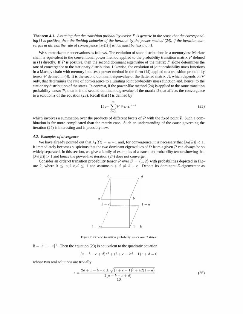
Consider an order-3 transition probability tensorP overS = 1, 2 with probabilities depicted in Fig-ure 2, where0 ≤ a, b, c, d ≤ 1 and assumea + d 6= b + c. Denote its dominantZ-eigenvector as

a b

c d

1− a 1− b

1− c 1− d

Figure 2: Order-3 transition probability tensor over 2 states.

z = [z, 1− z]⊤. Then the equation (23) is equivalent to the quadratic equation

(a− b− c+ d)z2 + (b + c− 2d− 1)z + d = 0

whose two real solutions are trivially

z =2d+ 1− b− c±

√(b+ c− 1)2 + 4d(1− a)

2(a− b − c+ d). (36)

10

Given values ofa, b, c, d, we are interested in the root satisfying0 ≤ z ≤ 1. By our theory, the correspondingΩ is given by

Ω = P ⊗12 z+ P ⊗13 z =

[b + c+ (2a− b− c)z 2d+ (b + c− 2d)z

(−2a+ b+ c)z + 2− b− c (2d− b− c)z − 2d+ 2

](37)

which has eigenvalues2 andb+ c− 2d+ 2(a− b− c+ d)z. Thus the second eigenvalue ofΩ is

1±√(b+ c− 1)2 + 4d(1− a),

depending on whichz is used.As an example, takea = 0 and b = c = d = 1. Thenz = −1+

√5

2 andλ2 = 1 −√5. In this

case, therefore, the power-like iteration cannot generatethe limiting stationary distribution vectorz because|λ2| > 1. In fact, our numerical experiment indicates that the iterates generated by the power-like methodwill have two accumulation points[1, 0]⊤ and [0, 1]⊤ and that the iterations move back and forth betweenthese two points. The dominant eigenvectorz is repelling equilibrium. By continuity, we see that a smallperturbation ofa, b, c, d while keeping them positive will not change the fact that thecorrespondingλ2 hasmodulus larger than 1. This observation suffices to establish the following result.

Theorem 4.2. There exists an open set of positive transition probabilitytensors with nonzero measure forwhich the power-like iteration (24) will not converge.

For instance8, takea = ǫ andb = c = d = 1− ǫ. Then the correspondingΩ(ǫ) has its second eigenvalue

1−√8ǫ2 − 12ǫ+ 5 < −1 for all 0 ≤ ǫ < 3−

√7

4 .

4.3. Deviation from true stationary distribution

Even if the given transition probability tensorP is such that the iteration (24) does converge to thedominantZ-eigenvector, we question the rationale of the assumption (21). Now that we understand that atrue Markov chain with memory should evolve with a dynamics for the sequence of vectorsx(t) in thesense of (8) and a dynamics for the sequence of tensorsΠt,t−1,...,t−m+2 in the sense of (11), we performsome numerical simulations to investigate whether there isa statistically significant deviation between resultsbased on this assumption and those from the true Markov process.

Denote the limiting joint probability mass function, the stationary distribution, and the dominantZ-eigenvector byΠ, x, andz, respectively. To simulate the general behavior of these quantities, we have totry out large samples of Markov chains. It will be sufficiently informative to consider the Markov chain withmemory 2. Toward this goal, the columns (in the sense of (5)) of the order-3 transition probability tensorPcan be thought of as coming from a uniform distribution over the simplex∆n−1.

Lemma 4.2. LetP be a random order-3 tensor with independent and identicallydistributed columns fromthe simplex∆n−1. Then the random vectorsx and z have the same expected value

E(x) = E(z) =

[1

n, . . . ,

1

n

]⊤. (38)

Also,

E(Π) =1

n21, (39)

where1 is then× n matrix with all ones.

8For this example, the valueγ defined by formula (2.2) in [12] is equal to 2, but we do not see convergence. This is in contrast to theassertion of Theorem 3.1 in [12].

11

x

0.12 0.14 0.16 0.18 0.2 0.22 0.24 0.26 0.28 0.3

z

0.12

0.14

0.16

0.18

0.2

0.22

0.24

0.26

0.28

0.3Correlation between x and z

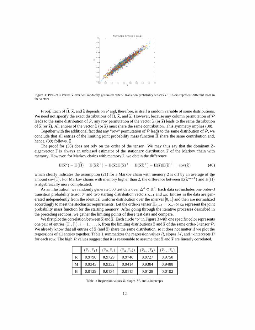
Figure 3: Plots ofz versusx over 500 randomly generated order-3 transition probability tensorsP . Colors represent different rows inthe vectors.

Proof. Each ofΠ, x, andz depends onP and, therefore, is itself a random variable of some distributions.We need not specify the exact distributions ofΠ, x, andz. However, because any column permutation ofPleads to the same distribution ofP , any row permutation of the vectorx (or z) leads to the same distributionof x (or z). All entries of the vectorx (or z) must share the same contribution. This symmetry implies (38).

Together with the additional fact that any “row” permutation ofP leads to the same distribution ofP , weconclude that all entries of the limiting joint probabilitymass functionΠ share the same contribution and,hence, (39) follows.

The proof for (38) does not rely on the order of the tensor. We may thus say that the dominant Z-eigenvectorz is always an unbiased estimator of the stationary distribution x of the Markov chain withmemory. However, for Markov chains with memory 2, we obtain the difference

E(x2)− E(Π) = E(xx⊤)− E(x)E(x)⊤ = E(xx⊤)− E(z)E(z)⊤ = cov(x) (40)

which clearly indicates the assumption (21) for a Markov chain with memory 2 is off by an average of theamountcov(x). For Markov chains with memory higher than 2, the differencebetweenE(xm−1) andE(Π)is algebraically more complicated.

As an illustration, we randomly generate 500 test data over∆4 ⊂ R5. Each data set includes one order-3

transition probability tensorP and two starting distribution vectorsx−1 andx0. Entries in the data are gen-erated independently from the identical uniform distribution over the interval[0, 1] and then are normalizedaccordingly to meet the stochastic requirements. Let the order-2 tensorΠ0,−1 = x−1⊗x0 represent the jointprobability mass function for the starting memory. After going through the iterative processes described inthe preceding sections, we gather the limiting points of these test data and compare.

We first plot the correlation betweenx andz. Each circle “o” in Figure 3 with one specific color representsone pair of entries(xi, zi), i = 1, . . . , 5, from the limiting distributionsx andz of the same order-3 tensorP .We already know that all entries ofx (andz) share the same distribution, so it does not matter if we plottheregressions of all entries together. Table 1 summarizes theregression valuesR, slopesM , andz-interceptsBfor each row. The highR values suggest that it is reasonable to assume thatx andz are linearly correlated.

(x1, z1) (x2, z2) (x3, z3)) (x4, , z4) (x5, , z5)

R 0.9790 0.9729 0.9748 0.9727 0.9750

M 0.9343 0.9332 0.9414 0.9384 0.9488

B 0.0129 0.0134 0.0115 0.0128 0.0102

Table 1: Regression valuesR, slopesM , andz-intercepts

12

0 0.01 0.02 0.03 0.04 0.05 0.06 0.07 0.080

10

20

30

40

50

60

70

80

90Histogram of ‖x− z‖

0 0.01 0.02 0.03 0.04 0.05 0.06 0.07 0.080

10

20

30

40

50

60

70

80

90Histogram of ‖x2

− z2‖

0.01 0.02 0.03 0.04 0.05 0.06 0.07 0.080

10

20

30

40

50

60

70

80Histogram of ‖x2

− Π‖

0 0.01 0.02 0.03 0.04 0.05 0.06 0.07 0.080

10

20

30

40

50

60

70

80

90Histogram of ‖z2 − Π‖

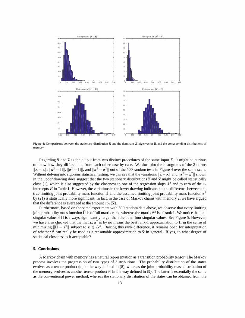
Figure 4: Comparisons between the stationary distributionx and the dominantZ-eigenvectorz, and the corresponding distributions ofmemory.

Regardingx andz as the output from two distinct procedures of the same inputP , it might be curiousto know how they differentiate from each other case by case. We thus plot the histograms of the 2-norms‖x − z‖, ‖x2 − Π‖, ‖z2 − Π‖, and‖x2 − z

2‖ out of the 500 random tests in Figure 4 over the same scale.Without delving into rigorous statistical testing, we can see that the variations‖z− x‖ and‖z2 − x

2‖ shownin the upper drawing does suggest that the two stationary distributionsz andx might be called statisticallyclose [1], which is also suggested by the closeness to one of the regression slopsM and to zero of thez-interceptsB in Table 1. However, the variations in the lower drawing indicate that the difference between thetrue limiting joint probability mass functionΠ and the assumed limiting joint probability mass functionz

2

by (21) is statistically more significant. In fact, in the case of Markov chains with memory 2, we have arguedthat the difference is averaged at the amountcov(x).

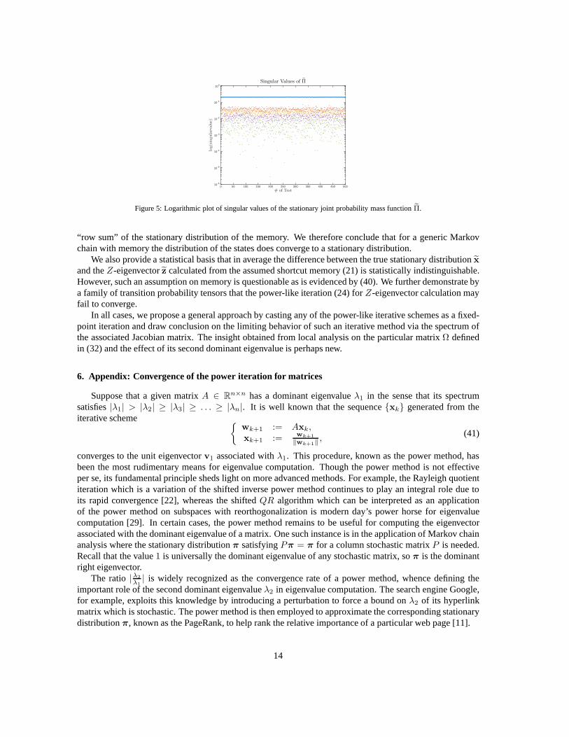
Furthermore, based on the same experiment with 500 random data above, we observe that every limitingjoint probability mass functionΠ is of full matrix rank, whereas the matrixz2 is of rank1. We notice that onesingular value ofΠ is always significantly larger than the other four singular values. See Figure 5. However,we have also checked that the matrixz

2 is by no means the best rank-1 approximation toΠ in the sense ofminimizing ‖Π − z

2‖ subject toz ∈ ∆4. Barring this rank difference, it remains open for interpretationof whetherz can really be used as a reasonable approximation tox in general. If yes, to what degree ofstatistical closeness is it acceptable?

5. Conclusions

A Markov chain with memory has a natural representation as a transition probability tensor. The Markovprocess involves the progression of two types of distributions. The probability distribution of the statesevolves as a tensor product⊛1 in the way defined in (8), whereas the joint probability mass distribution ofthe memory evolves as another tensor product in the way defined in (9). The latter is essentially the sameas the conventional power method, whereas the stationary distribution of the states can be obtained from the

13

# of Test0 50 100 150 200 250 300 350 400 450 500

log(singu

larvalue)

10 -6

10 -5

10 -4

10 -3

10 -2

10 -1

100Singular Values of Π

Figure 5: Logarithmic plot of singular values of the stationary joint probability mass functionΠ.

“row sum” of the stationary distribution of the memory. We therefore conclude that for a generic Markovchain with memory the distribution of the states does converge to a stationary distribution.

We also provide a statistical basis that in average the difference between the true stationary distributionx

and theZ-eigenvectorz calculated from the assumed shortcut memory (21) is statistically indistinguishable.However, such an assumption on memory is questionable as is evidenced by (40). We further demonstrate bya family of transition probability tensors that the power-like iteration (24) forZ-eigenvector calculation mayfail to converge.

In all cases, we propose a general approach by casting any of the power-like iterative schemes as a fixed-point iteration and draw conclusion on the limiting behavior of such an iterative method via the spectrum ofthe associated Jacobian matrix. The insight obtained from local analysis on the particular matrixΩ definedin (32) and the effect of its second dominant eigenvalue is perhaps new.

6. Appendix: Convergence of the power iteration for matrices

Suppose that a given matrixA ∈ Rn×n has a dominant eigenvalueλ1 in the sense that its spectrumsatisfies|λ1| > |λ2| ≥ |λ3| ≥ . . . ≥ |λn|. It is well known that the sequencexk generated from theiterative scheme

wk+1 := Axk,

xk+1 := wk+1

‖wk+1‖ ,(41)

converges to the unit eigenvectorv1 associated withλ1. This procedure, known as the power method, hasbeen the most rudimentary means for eigenvalue computation. Though the power method is not effectiveper se, its fundamental principle sheds light on more advanced methods. For example, the Rayleigh quotientiteration which is a variation of the shifted inverse power method continues to play an integral role due toits rapid convergence [22], whereas the shiftedQR algorithm which can be interpreted as an applicationof the power method on subspaces with reorthogonalization is modern day’s power horse for eigenvaluecomputation [29]. In certain cases, the power method remains to be useful for computing the eigenvectorassociated with the dominant eigenvalue of a matrix. One such instance is in the application of Markov chainanalysis where the stationary distributionπ satisfyingPπ = π for a column stochastic matrixP is needed.Recall that the value1 is universally the dominant eigenvalue of any stochastic matrix, soπ is the dominantright eigenvector.

The ratio |λ2

λ1| is widely recognized as the convergence rate of a power method, whence defining the

important role of the second dominant eigenvalueλ2 in eigenvalue computation. The search engine Google,for example, exploits this knowledge by introducing a perturbation to force a bound onλ2 of its hyperlinkmatrix which is stochastic. The power method is then employed to approximate the corresponding stationarydistributionπ, known as the PageRank, to help rank the relative importanceof a particular web page [11].

14

A typical way in numerical linear algebra to argue the rate ofconvergence of the power method (41) fora matrixA is to assume the existence of a basis of eigenvectorsv1, . . . ,vn

9. Upon expanding the startingvector

x0 =

n∑

i=1

civi

in terms of the basis, the iteratexk can then be expressed as

xk =

c1λk1

(v1 +

∑n

i=2 ci

(λi

λ1

)kvi

)

∥∥∥∥c1λk1

(v1 +

∑n

i=2 ci

(λi

λ1

)kvi

)∥∥∥∥.

Hence, we see that the non-essential quantities decay at a rate of approximately|λ2

λ1|. Such a loose argument

is conceptually acceptable, but can hardly be generalized to tensors because the tensor space may not have abasis of eigenvectors. An alternative argument is to use fixed-point theory. We have done so for tensors inSection 4.1. We now demonstrate how it applied to matrices.

Let Sn−1 denote the unit sphere inRn. Without loss of generality, supposeA is nonsingular. Define amapf : Sn−1 → Sn−1 by

f(x) =Ax

‖Ax‖2(42)

where the normalization by the 2-norm is only for convenience. The power method can be cast as the fixed-point iteration

xk+1 = f(xk). (43)

Sincef is a continuous function mapping from a compact set into itself, by the Brouwer fixed-point theorem,there is a pointx ∈ Sn−1 such thatf(x) = x. In particular, by switching the sign if necessary, we mayassume that the dominant unit eigenvectorv1 is one such a fixed point. We now describe the local behaviorof f nearbyv1.

Forxk sufficiently nearv1, we have the linear approximation

xk+1 − v1 = f(xk)− f(v1) ≈ Df(v1)(xk − v1), (44)

where it is easy to see that the Jacobian matrix off is given by

Df(x) =A

‖Ax‖2− Axx⊤A⊤A

‖Ax‖32. (45)

It follows that atv1 we have

Df(v1) =1

|λ1|(I − v1v

⊤1 )A. (46)

Obviously,v⊤1 Df(v1) = 0. Let wi ∈ Cn be any eigenvector ofA⊤ associated with eigenvalueλi ∈ C,

i = 2, . . . n. Then it is known thatw⊤i v1 = 0 sinceλi 6= λ1. Thusw⊤

i Df(v1) =λi

|λ1|w⊤i . In all, we make

the following conclusion.

Lemma 6.1. The spectrum of the Jacobian matrixDf(v1) is precisely0, λ2

|λ1| ,λ3

|λ1| , . . . ,λn

|λ1|

.

9In case that the matrixA is defective, some arguments can still be made. See, for example, detailed discussions in the classic book[7]. The local analysis presented in this section, however,does not require such a basis.

15

As a simple demonstration, consider the generic case that the matrixDf(v1) has a spectral decompositionDf(v1) = U−1ΛU . Then by (44) we can write

U(xk+1 − v1) ≈ ΛU(xk − v1), (47)

implying that

‖U(xk+1 − v1)‖∞ ≈∣∣∣∣λ2

λ1

∣∣∣∣ ‖U(xk − v1)‖∞. (48)

It is in this sense that oncexk is sufficiently close tov1, thenxk+1 is even closer and that the rate of linearconvergence is given by the ratio|λ2

λ1|.

References

[1] T. BATU , L. FORTNOW, R. RUBINFELD, W. D. SMITH , AND P. WHITE, Testing that distributions areclose, in 41st Annual Symposium on Foundations of Computer Science (Redondo Beach, CA, 2000),IEEE Comput. Soc. Press, Los Alamitos, CA, 2000, pp. 259–269.

[2] D. CARTWRIGHT AND B. STURMFELS, The number of eigenvalues of a tensor, Linear Algebra Appl.,438 (2013), pp. 942–952.

[3] K. CHANG, L. QI , AND T. ZHANG, A survey on the spectral theory of nonnegative tensors, Numer.Linear Algebra Appl., 20 (2013), pp. 891–912.

[4] K. C. CHANG AND T. ZHANG, On the uniqueness and non-uniqueness of the positivez-eigenvectorfor transition probability tensors, J. Math. Anal. Appl., 408 (2013), pp. 525–540.

[5] Z. CHEN, L. QI , Q. YANG, AND Y. YANG, The solution methods for the largest eigenvalue (singularvalue) of nonnegative tensors and convergence analysis, Linear Algebra Appl., 439 (2013), pp. 3713–3733.

[6] H. G. DIAZ , R. MOLINA , AND E. URIARTE, Stochastic molecular descriptors for polymers. 1.modelling the properties of icosahedral viruses with 3d-markovian negentropies, Polymer, 45 (2004),pp. 3845 – 3853.

[7] D. K. FADDEEV AND V. N. FADDEEVA, Computational methods of linear algebra, Translated byRobert C. Williams, W. H. Freeman and Co., San Francisco-London, 1963.

[8] D. F. GLEICH, L.-H. L IM , AND Y. Y U, Multilinear PageRank, SIAM J. Matrix Anal. Appl., 36 (2015),pp. 1507–1541.

[9] Y. H UA , X. L IU , AND H. JIANG, ANTELOPE: a semantic-aware data cube scheme for cloud datacenter networks, IEEE Trans. Comput., 63 (2014), pp. 2146–2159.

[10] T. G. KOLDA AND B. W. BADER, Tensor decompositions and applications, SIAM Rev., 51 (2009),pp. 455–500.

[11] A. N. LANGVILLE AND C. D. MEYER, Google’s PageRank and beyond: the science of search enginerankings, Princeton University Press, Princeton, NJ, 2012. Paperback edition of the 2006 original.

[12] W. L I AND M. K. NG, On the limiting probability distribution of a transition probability tensor, LinearMultilinear Algebra, 62 (2014), pp. 362–385.

[13] L.-H. L IM , Singular values and eigenvalues of tensors: A variational approach, in Proceedings of1st IEEE International Workshop on Computational Advancesof Multi-Tensor Adaptive Processing(CAMSAP), Puerto Vallarta, December 13–15 2005, pp. 129–132.

16

[14] L.-H. L IM , M. K. NG, AND L. QI, The spectral theory of tensors and its applications, Numer. LinearAlgebra Appl., 20 (2013), pp. 889–890.

[15] Y. L IU , G. ZHOU, AND N. F. IBRAHIM , An always convergent algorithm for the largest eigenvalue ofan irreducible nonnegative tensor, J. Comput. Appl. Math., 235 (2010), pp. 286–292.

[16] I. L. M ACDONALD AND W. ZUCCHINI, Hidden Markov and other models for discrete-valued timeseries, vol. 70 of Monographs on Statistics and Applied Probability, Chapman & Hall, London, 1997.

[17] R. S. MAMON AND R. J. ELLIOTT , eds.,Hidden Markov models in finance, International Series inOperations Research & Management Science, 104, Springer, New York, 2007.

[18] , eds.,Hidden Markov models in finance, International Series in Operations Research & Manage-ment Science, 209, Springer, New York, 2014. Further developments and applications. Vol. II.

[19] S. S. MELNYK , O. V. USATENKO, AND V. A. YAMPOL′SKII, Memory functions of the additive Markovchains: applications to complex dynamic systems, Phys. A, 361 (2006), pp. 405–415.

[20] S. L. NARASIMHAN , J. A. NATHAN , AND K. P. N. MURTHY, Can coarse-graining introduce long-range correlations in a symbolic sequence?, EPL (Europhysics Letters), 69 (2005), p. 22.

[21] M. NG, L. QI , AND G. ZHOU, Finding the largest eigenvalue of a nonnegative tensor, SIAM J. MatrixAnal. Appl., 31 (2009), pp. 1090–1099.

[22] B. N. PARLETT, The Rayleigh quotient iteration and some generalizations for nonnormal matrices,Math. Comp., 28 (1974), pp. 679–693.

[23] L. QI, Eigenvalues and invariants of tensors, J. Math. Anal. Appl., 325 (2007), pp. 1363–1377.

[24] A. E. RAFTERY, A model for high-order Markov chains, J. Roy. Statist. Soc. Ser. B, 47 (1985), pp. 528–539.

[25] O. ROSE, A memory markov chain model for vbr traffic with strong positive correlations,tech. report, Institute of Computer Science, University ofWüzburg, 1999. downloadable athttp://citeseerx.ist.psu.edu/viewdoc/download?doi=10.1.1.8.9230&rep=rep1&type=pdf.

[26] E. ROSOLOWSKY, Statistical analyses of data cubes, in Statistical challenges in modern astronomy V,vol. 209 of Lecture Notes in Statist., Springer, New York, 2013, pp. 367–382.

[27] V. SOLOVIEV , V. SAPTSIN, AND D. CHABANENKO, Markov Chains application to the financial-economic time series prediction, ArXiv e-prints, (2011).

[28] O. V. USATENKO, V. A. YAMPOL’ SKII , K. E. KECHEDZHY, AND S. S. MEL’ NYK , Symbolic stochas-tic dynamical systems viewed as binary N -step markov chains, Phys. Rev. E, 68 (2003), p. 061107.

[29] D. S. WATKINS, Understanding theQR algorithm, SIAM Rev., 24 (1982), pp. 427–440.

[30] L. ZHANG AND L. QI, Linear convergence of an algorithm for computing the largest eigenvalue of anonnegative tensor, Numer. Linear Algebra Appl., 19 (2012), pp. 830–841.

[31] G. ZHOU, L. QI , AND S.-Y. WU, Efficient algorithms for computing the largest eigenvalue of a non-negative tensor, Front. Math. China, 8 (2013), pp. 155–168.

17