Markov Decision Processes for Screening and …btdenton.engin.umich.edu/wp-content/uploads/sites/138/...Markov Decision Processes for Screening and Treatment of Chronic Diseases 3

Markov Decision Processes for Screening andTreatment of Chronic Diseases

Lauren N. Steimle and Brian T. Denton

Abstract In recent years, Markov decision processes (MDPs) and partially obser-able Markov decision processes (POMDPs) have found important applications tomedical decision making in the context of prevention, screening, and treatment ofdiseases. In this chapter, we provide a review of state-of-the-art models and meth-ods that have been applied to chronic diseases. We provide a thorough tutorial abouthow to formulate and solve these MDPs and POMDPs emphasizing some of thechallenges specific to chronic diseases. Then, we illustrate important considerationsfor model formulation and solution methods through two examples. The first exam-ple is an MDP model for optimal control of drug treatment decisions for controllingthe risk of heart disease and stroke in patients with type 2 diabetes. The secondexample is a POMDP model for optimal design of biomarker-based screening poli-cies in the context of prostate cancer. We end the chapter with a discussions of thechallenges of using MDPs and POMDPs for medical contexts and describe someimportant future directions for research.

1 Introduction

Chronic diseases are the leading cause of death and disablement in many countries.Although these diseases cannot be cured, they can be controlled by screening andtreatment. Clinicians are tasked with deciding which screening and treatment op-tions are most beneficial for a patient. These decisions are made sequentially overlong periods of a patient’s life and are made in an uncertain environment. Although

Lauren N. SteimleDepartment of Industrial and Operations Engineering, University of Michigan1205 Beal Ave, Ann Arbor, MI 48109, e-mail: [email protected]

Brian T. DentonDepartment of Industrial and Operations Engineering, University of Michigan1205 Beal Ave, Ann Arbor, MI 48109, e-mail: [email protected]

1

[email protected]

[email protected]

2 Lauren N. Steimle and Brian T. Denton

clinicians can observe a patient’s current health or test results, there is uncertainty inthe future progression of the disease, the effect of treatment on the patient, and eventhe correctness of test results. Medical decisions have grown even more complicateddue to the aging patient population. Older patients often have multiple chronic con-ditions, and treatment for one condition may worsen another. Health care providershave recognized these growing problems and have responded with increased expen-ditures on data collection and tracking systems. With the growth in medical datacomes the need for analytical methodology to convert these data into information.Recently, operations research methods have proven to be powerful tools to analyzethese data to guide screening and treatment decisions.

Markov decisions processes (MDPs) are increasingly being used in the analysisof medical decisions, especially chronic disease screening and treatment decisions.Both screening and treatment decisions are characterized by large state spaces thatdefine the severity of the disease, patient-specific clinical risk factors, and med-ication histories, and these decisions have uncertain outcomes due to differencesamong patients such as genetic, environmental, and dietary factors. The frameworkof MDPs lends itself well to these decisions since they are made sequentially overtime in a fundamentally stochastic environment. Further, partially observable MDPs(POMDPs) are useful for studying systems in which the true state of the system isnot known exactly, which is usually the case when screening for a chronic disease.

Modeling screening and treatment decisions using MDPs is not without its chal-lenges. These clinical decisions take place over long periods (sometimes decades)under constraints due to medication conflicts, clinical practice requirements, or bud-get constraints. Furthermore, the influence of patient’s treatment and screening his-tory on future decisions leaves these models subject to the curse of dimensionalitydue to dramatic increase in the size of the state space that can be caused by this his-tory dependence. As a result, optimization of the stochastic and sequential decisionmaking process gives rise to computationally-intensive problems that are difficult tosolve, even with state-of-the-art algorithms and computing resources. Fortunately,many of these problems have promising structural properties that can be exploitedto achieve meaningful theoretical insights and lead to efficient exact and/or approx-imation methods.

The remainder of this chapter is organized as follows: in Section 2, we discusssome applications of MDPs to chronic diseases. In Section 3, we discuss how toformulate an MDP/POMDP model in the context of chronic disease and solutionmethods that can be used to determine optimal policies for these models. In Sec-tions 4 and 5, we give in-depth descriptions of an MDP used for the treatment oftype 2 diabetes and a POMDP model used for screening of prostate cancer. We endthe chapter with discussion of the open challenges that need to be addressed whenusing MDP/POMDP models for chronic diseases in Section 6 and some concludingremarks in Section 7.

Markov Decision Processes for Screening and Treatment of Chronic Diseases 3

2 Background on Chronic Disease Modeling

Surveys of operations research applications in healthcare can be found in [1, 2, 3].Many of the examples are in the context of healthcare operations management,which has been an important application area for decades. In contrast to operationsmanagement, the study of disease screening and treatment policies has a shorterhistory and is confined to a relatively small, but fast growing, number of topic areasincluding liver and kidney transplant decisions [4, 5, 6, 7, 8, 9, 10], breast cancerscreening [11, 12], intensity modulated radiation therapy [13, 14, 15] and brachy-therapy [16] for cancer treatment, the treatment of HIV [17], and public policy de-cisions related to the transmission of communicable diseases [18, 19].

MDPs can be used to study sequential decisions made in uncertain environments,which is why they are so powerful for the analysis of chronic disease screening andtreatment. Before describing how these models are formulated, we provide somemotivation for the study of MDPs in the context of chronic diseases by giving thefollowing examples of clinically-relevant questions that have been answered:

• At what point should a patient with HIV initiate highly active antiretroviral ther-apy (HAART)?Human Immunodeficiency Virus (HIV) is a virus that attacks the CD4 whiteblood cells to the point the body can no longer protect itself against infectionsand disease. Acquired Immune Deficiency Syndrome (AIDS) is caused by HIVand eventually leads to death. Once someone acquires HIV, the virus will remainin the body for the remainder of that person’s life. Highly active antiretroviraltherapy (HAART) prevents the virus from multiplying and is the standard treat-ment for HIV patients. However, it was debated whether to “hit early, hit hard”with HAART, as was the treatment model in the late 1990s, or to wait until theCD4 count falls between 200 and 350 as suggested by more recent guidelines.The authors of [17] used an infinite-horizon MDP with the objective of maximiz-ing a patient’s total expected lifetime or quality-adjusted lifetime to answer thisopen question. The states of the MDP were defined by a patient’s CD4 count,and at each monthly decision epoch, the decision was to “initiate HAART” or“wait to initiate HAART”. The authors proved that there exists a control-limitpolicy, which initiated therapy if and only if the CD4 count falls below a certainthreshold. The optimal policy suggested that HAART should be initiated earliersupporting the “hit early, hit hard” approach to HIV treatment.

• When should women receive mammograms to screen for breast cancer?Breast cancer is the second leading cause of cancer death for women in the UnitedStates. Detecting breast cancer in its early stages allows for treatment and de-creases the risk of a breast cancer mortality. A mammogram is an x-ray imageof the breast that can be used to detect breast cancer before a woman developssymptoms. If a mammogram shows a suspicious area, a biopsy can be performedto determine if the abnormality is cancer. While these tests are useful in deter-mining if a patient has cancer, they are not perfect. Mammograms can lead to ra-


diation exposure and pain, and biopsies are an invasive procedure associated withpain and anxiety. Further, mammograms can give false negative and false posi-tive results. There are significant differences between the guidelines published byhealth organizations within the U.S. and worldwide. The authors of [20] created afinite-horizon POMDP model to determine personalized mammography screen-ing policies that depend on a woman’s personal risk factors and past screeningresults. The unobservable states represent which stage of cancer the patient has -no cancer, noninvasive cancer, invasive cancer, invasive cancer under treatment,or death. The actions of this POMDP are “wait” and “mammography”. If theaction chosen is mammography, the decision maker can observe a positive ornegative mammogram result. If the action is to wait, the patient can give a self-detection result that is either positive or negative. If a mammogram is positive,the patient will get a biopsy, and if a self-detection is positive, the patient will geta mammogram. With these observations in mind, the decision maker can updateher belief state which describes the probability that a patient is in any given stategiven the history of mammogram results. The authors find that a control-limitpolicy exists that depends on the risk of noninvasive and invasive cancers andthat a patient’s screening history may affect the decision of whether to perform amammography or not.

• When should a patient with end-stage liver disease accept a living-donor trans-plant? For patients with end-stage liver diseases such as primary biliary cirrho-sis, hepatitis C, and acute failure (fulminants) disease, organ transplantation is theonly treatment option. Provided that a patient with end-stage liver disease has awilling living donor, it might seem the patient should receive a transplant as soonas possible. However, depending on the quality of the match with the donor andthe current health of the patient, this decision might give a lower expected totallifetime for the patient compared with the decision to wait. To analyze this situ-ation, the authors of [4] create an infinite-horizon MDP model in which the statespace is represented by a patient’s “Model For End-Stage Liver Disease”(MELD)score. The MELD score quantifies the severity of end-stage liver disease basedon laboratory results and is used for the purpose of transplant decisions. HigherMELD scores are associated with more severe liver disease. At each daily deci-sion epoch, the actions are “transplant” and “wait”. If the decision is to wait,the patient will receive a reward of one life day and then progress probabilis-tically among the health states or die. Once the decision to transplant is made,the patient transitions into an absorbing state and receives a reward correspond-ing to the expected life days associated with the health of the patient at the timeof the transplantation and the quality of the match with the donor. The authorsprove that the optimal policy has a control-limit structure in which the patientwill only accept a liver of a given quality if her MELD score is worse than thecontrol-limit. For example, a MELD score of 20 is the control-limit given thatthe quality of the match has a score of 4. Therefore, a patient with a MELD scoreof 25 should accept this liver to transplant while a patient with a MELD score of15 should wait to transplant.


These examples illustrate some treatment and screening decisions that can beanalyzed using MDPs. More examples of MDPs used in medicine can be found inthe reviews by [21, 22]. This chapter differs from these previous reviews in that weprovide an in-depth discussion of how to formulate MDP models for chronic diseasescreening and treatment problems. We also provide detailed examples that illustrateMDP model formulation, validation, solutions, and interpretation of results. Finallywe compare and constrast perfectly observable and imperfectly observable contexts.With this motivation, we will proceed to more formally describe how MDPs can beformulated to generate insights for screening or treating a chronic disease.

3 Modeling Framework for Chronic Diseases

The remainder of this chapter will focus on the modeling framework for MDPsspecifically in the context of screening and treatment applications. This section willprovide a tutorial on how to formulate, solve, and validate these models. In thefollowing sections, we will provide several examples to illustrate the developmentof the formulation and potential challenges faced by researchers.

3.1 MDP and POMDP Model Formulation

To build an MDP model of a chronic disease treatment process, one must define thedecision epochs/ time horizon, state space, action space, transition probabilities,and rewards as they relate to the specific disease and screening/treatment optionsbeing considered.

Decision Epochs / Time Horizon: Treatment and screening decisions are madeat each decision epoch. The length of time between decision epochs for a chronicdisease model usually corresponds to the time between treatment and/or screeningdecisions made by the clinician. For instance, in the case of liver transplantation,decisions about whether to transplant or not could be made daily, while in the caseof type 2 diabetes, decisions about which medications to initiate are more likely tobe made less frequently (e.g. every 6 or 12 months based on clinical guidelines). De-termining the ideal time interval requires some understanding of the disease contextand clinical practice.

Another modeling choice is whether to consider a finite-horizon formulation, inwhich there are a finite number of decision epochs, or an infinite-horizon formula-tion. While the patient will die in a finite amount of time, some researchers use aninfinite-horizon approach for treatment decisions when the time between epochs isshort relative to the length of the horizon over which decisions are made. For ex-ample, in organ transplantation, if the decision epochs are daily, it may be suitableto model use an infinite-horizon. Usually infinite-horizon problems are associated


with an absorbing state that is reached with probability 1, such as a post-treatmentabsorbing state. Moreover, infinite-horizon models are often stationary, i.e., modelparameters do not vary over time.

State Space: The state space of the model represents the information that wouldbe useful to a clinician when making decisions regarding a patient. A state vectortypically includes the patient’s health status, demographic information, and relevantmedical history.

A patient’s health status is usually defined by a number of clinical risk factorsor a risk score that can be used by clinicians to predict the severity of a disease orthe likelihood of developing a disease. For example, when determining whether ornot to transplant a liver, clinicians consider a patient’s MELD score which dependson a number of laboratory values that are useful in determining the severity of liverdisease. While MELD scores are integer-valued, other metabolic risk factors, suchas body mass index (BMI), are continuous. Most MDP models used for medical de-cisions discretize the true continuous state space to reduce the computation neededto solve the model. A finer discretization may be more representative of the truecontinuous state space, but it also increases the size of the state space and there-fore the computation required to solve the model. Further, a finer discretization willdecrease the number of observed transitions for some state-action pairs introducingmore sampling error into the estimates of the transition probabilities. [23] providesa discussion of the trade-off between the model error introduced with a more coarsediscretization and the sampling error that is associated with a finer discretization.

A patient’s demographic information can be important for defining the state spaceof a model. The dynamics of some diseases vary depending on the demographics ofthe patient such as age and race. For example, [11] considers age because olderwomen are at higher risk for developing breast cancer, but breast cancer is lessaggressive in these women. These dynamics may be important in determining theoptimal treatment or screening policies, but incorporating this information mightrequire formulation and validation of unique models for these different populations.

Information about a patient’s medical history, such as medication history or his-tory of adverse events, may affect treatment decisions. For example, once a patienthas had one heart attack, she is at increased risk to have a second heart attack. Al-though this history is important, MDP models require that the transitions amongstates must maintain the Markov property, i.e, the next state may only depend on thecurrent state and the action taken. To maintain this property, it is necessary to in-corporate any necessary history of the patient into the state definition. For example,the state definition may include which medications a patient has already initiated orhow many adverse events the patient has already had.

In most MDP models of chronic disease, there is an absorbing state representingmajor complication and/or death. In some models, there are separate death statesdepending on the cause of death (e.g. death from a heart attack, death from othercauses). It may be necessary to use more than one absorbing state when absorbingstates that are reachable from a given health state vary or when rewards vary depend-ing on the absorbing state that is reached. Defining the state space is closely tied to


what sources exist to estimate transition probabilities, such as statistical survivalmodels or patient data.

POMDPs are a generalization of MDPs in which the decision maker does notknow the state of the system with certainty. This generalization is particularly usefulwithin the context of chronic disease, because often clinicians cannot be 100% sureof the health state of their patients. While screening and diagnostic tests providevaluable information, these tests sometimes give false positive and false negativetest results which leaves the true health state of the patient uncertain. In a POMDP,the state space is defined by a core process and an observation process (also referredto as a message process). With respect to chronic diseases, the core process corre-sponds to the true health of a patient, such as cancer-free, has non-invasive cancer,has invasive cancer, in treatment, or dead. To a clinician, the first three states are un-observable, meaning that the clinician cannot know with certainty the true state ofthe patient. The observation process corresponds to observable test results, such as amammogram. The core process and the observation process are tied together prob-abilistically through an information matrix with elements that define probabilitiesof a particular observation given a particular core state. For example, the decisionmaker may know the true and false positive and negative rates of a biopsy based onclinical studies. Using Bayesian updating, the relationship between the core and ob-servation processes and the observed test result can be used to create a belief state.The belief state is a probability distribution describing the believed true state of thesystem based on the decision maker’s past observations. For additional details spe-cific to POMDPs, the reader is referred to [24, 25].

Action Space: To identify the action space of the MDP, one must identify whichscreening or treatment options to consider. In the case where there is a clear “best”treatment option, the action space might be only two actions: treat the patient withthe best therapy or wait. These are typically referred to as optimal stopping-timeproblems in the literature, because the decision maker aims to choose the optimaltime to stop the process and enter the absorbing post-treatment state. For instance,deciding when to transplant an organ is usually a stopping-time problem with theaction space being transplant or wait to transplant.

For some diseases, it is not clear which therapy is the best or different therapiesmay be used together to treat the patient. In these cases, the action space can growquite large because of the combinatorial nature of the actions. For example, if M ={m1,m2, ...,mn} is a set of different drugs that can be used in any combination totreat a patient, the action space becomes 2M (the power set of M) and the size of theaction space grows exponentially in the number of treatments considered.

In a POMDP model, the decision maker can take actions to gain informationabout the state of the system. For example, screening decisions can be modeled us-ing POMDP models where the action space might represent the different types ofscreening tests available. Performing a screening test may not change the naturalprogression of the disease, but it can provide the decision maker with valuable in-formation about the true health state of the patient, which in turn may be used to


decide whether to do more invasive testing such as biopsy or radiologic imaging.

Transition Probabilities: The transition probabilities in a MDP model of chronicdisease usually describes the progression of the disease with and without treatment,the probability of an adverse event, and the probability of death. To describe theprogression of a disease, a key step is to build a natural history model. The naturalhistory model describes how the disease progresses under no treatment. Creatingthis model can be challenging because medical records will only contain data aboutpatients who have been diagnosed and treated for the disease. To build a naturalhistory model, one can use longitudinal data to estimate the effects of treatmentby observing measurements of risk factors before and after a patient starts the treat-ment. In this way, one could estimate how the disease would progress if no treatmentwas given to a patient. It is important to note that measures such as this can be af-fected by bias associated with patterns that influence which patients are referred fortreatment. For example, patients who initiate blood pressure lowering medicationswould typically have higher than normal blood pressure and may exhibit greaterrelative reduction in blood pressure than the general population.

When there is a clear “best” therapy, as is the case in optimal stopping-timeproblems, the modeler is not concerned with the effect of treatment on the transi-tion probabilities. Upon initiating treatment, the patient will transition to an absorb-ing state representing post-treatment with probability 1. In other cases, the modelermust consider how treatment affects the transition probabilities. Presumably, initiat-ing treatment will lower the probability of having an adverse event or dying from thedisease. A recent proliferation of statistical models for estimating the risk of chronicdisease complications can provide these inputs for MDPs. For instance, statisticalmodels for type 2 diabetes include: the Framingham model [26, 27, 28], the UKPDSmodel [29, 30, 31, 32], and the ACC/AHA pooled risk calculator [33]. These mod-els predict the probability of diabetes complications such as cardiovascular events(stroke and coronary heart disease), kidney failure, and blindness. Inputs includegender, race, family history, and metabolic factors like cholesterol, blood pressure,and blood glucose. Treatment can affect some of the inputs to these models andtherefore can affect the transition probability to an adverse event state.

Another key input to an MDP model is the probability associated with transition-ing to the death state. The probability of death caused by something other than thedisease of interest is called all other cause mortality. All other cause mortality canhave a large impact on treatment decisions. As all other cause mortality increases,treatment decisions become less beneficial since the probability of dying from theparticular disease of focus for the MDP is not as likely. This is particularly impor-tant for chronic diseases that progress slowly. For example, the American UrologyAssociation recommends not screening men for prostate cancer after age 75 becausemen who have not been diagnosed with prostate cancer by this age are not likely todie from this slowly progressing disease. Estimates for all other cause mortality cantypically be found using mortality tables from the Centers for Disease Control andPrevention (CDC).


Rewards: The rewards and costs in a chronic disease MDP model may be associatedwith the economic and health implications associated with treatment and screen-ing policies. To determine the relevant rewards and costs, one must identify theperspective of the decision maker: patient, third-party payer (e.g. Blue Cross BlueShield, Medicare), or a societal perspective that combines these different perspec-tives. Treating or screening a patient for a chronic disease will offer some reward tothe patient, such as a potentially longer life. However, these benefits come at some“cost” to the patient, whether it be a reduction in quality of life, such as side effectsdue to medication or discomfort due to a screening test, or a financial cost, suchas medication or hospitalization expenses. Health services researchers typically usequality-adjusted life years (QALYs) to quantify the quality of a year of life with thediscomfort due to medical interventions. A QALY of 1 represents a patient in perfecthealth with no disutility due to medical interventions and side effects of treatment.As the patient’s quality of life decreases, whether from medication side effects ordisablement from a disease, the patient’s QALY value will tend towards zero. (Thereader is referred to [34] for a review of QALYs and other quality of life measures.)Some MDP models are only concerned with maximizing a patient’s QALYs. Othermodels take a societal perspective and attempt to balance the health benefits of treat-ment with the corresponding monetary costs of medical interventions. To balancethese competing objectives, a common approach is to use a willingness to pay fac-tor, which assigns a monetary value to a QALY. Values of $50,000 and $100,000per QALY have commonly been used in the literature; however, the exact value touse is often debated [35].

MDPs are rather data-intensive due to the need for transition probabilities andrewards for each state-action pair. However, after gleaning these inputs from theliterature or longitudinal patient data, solving these MDPs can generate meaningfulinsights into how and when to screen for and treat chronic diseases.

3.2 Solution Methods and Structural Properties

Various algorithms have been developed for the use of solving MDPs and POMDP.The appropriate method for solving an MDP depends on whether the MDP is for-mulated as an infinite-horizon or finite-horizon problem and the size of the state andaction spaces. Methods such as policy iteration, value iteration, and linear program-ming have been used to solve infinite-horizon problems, while backwards inductionis typically used to solve finite-horizon problems. One problem with MDP formu-lations is that they are subject to the curse of dimensionality. This is seen in MDPsfor chronic disease where the size of the state space grows exponentially with thenumber of health risk factors defining the state. To circumvent this problem, ap-proximation algorithms can be used. There has been a great amount of researchon approximate dynamic programming in general, but these approaches tend to be


highly context dependent and very little work has been done in the context of chronicdisease. [36, 37] provide a thorough review of approximation methods of MDPs.

Many MDP models for chronic diseases have certain structural properties thatcan be exploited for computational gains. One such property is the increasing failurerate (IFR) property describing the transition probability matrices. In the context ofchronic diseases, the IFR property means that the worse the health status of thepatient is, the more likely that the health status will become even worse. Usuallythis ordering naturally follows the severity of the chronic disease, with the orderingof the states defined by a patient’s health status. For certain optimal stopping-timeproblems, it has been shown that the IFR property together with some additional(and nonrestrictive) conditions guarantees an optimal threshold policy (see Chapter4 of [38]). These conditions have be used in the context of HIV [17], liver disease[4], and type 2 diabetes [39] to prove the existence of an optimal control-limit policy.A control-limit policy is one in which one action is used for all states below a certainvalue (e.g. wait to transplant if the MELD score is below 25) and another action forall states above a certain value (e.g. transplant if the MELD score is at least 25).Proving the existence of a control-limit policy can decrease the computational effortrequired to solve the MDP model, since the value function does not need to beexplicitly calculated for every state/action pair.

POMDPS are generally much more challenging to solve than MDPs. Earlymethodological studies focused on exact methods that exploit the fact that the opti-mal value function for a POMDP is convex, and in the finite-horizon case it is piece-wise linear and expressible using a finite set of supporting hyperplanes. The firstexact method was provided by [40]. The authors proposed an iterative approach togenerate supporting hyperplanes at each decision epoch. Due to exponential growthin the number of hyperplanes with respect to the number of decision epochs andobservations and the fact that many of the hyperplanes are dominated, the authorsfurther proposed an approach to reduce the number of hyperplanes to a minimal setusing a linear programming formulation to identify dominated hyperplanes. Manyauthors have built on this early approach by developing more efficient ways of prun-ing unnecessary hyperplanes, including incremental pruning [41] and the witnessmethod [42]. Exact methods are generally limited to small POMDPs. A well-knownapproximation approach for moderate-sized POMDPs is based on discretizing thecontinuous belief state to obtain an approximate finite state MDP. One of the firstproposed approaches was the fixed-grid algorithm proposed by [43]. Many enhance-ments, including variable grid based approaches have built on this early idea. Thereader is referred to [44] for discussion of finite grid based approaches. Grid basedmethods are limited in their applicability to large-scale POMDPs. For this reason, itis often necessary to develop approximation methods tailored to particular applica-tions.


3.3 Model Validation

Once an MDP has been solved, it is critical to determine whether the results of themodel are valid. Below are some common ways to validate MDP models for chronicdiseases.

Expert Opinion: After the MDP has been solved, one can seek the opinion of anexpert in the field, such as a clinician or a health services researcher, to determine ifthe results of the model are realistic. This form of validation is not very strong sinceit is subjective. Some experts may have differing opinions of whether the model re-sults are actually valid. However, this form of validation is probably the easiest touse and can be a first step in validating the model before turning to more objectiveprocedures.

Independent Study: To validate an MDP, one could compare the results to a modeldeveloped independently. For instance, an alternative stochastic model could becompared to the MDP using a reference policy (e.g. an existing screening or treat-ment guideline.)

Retrospective validation: Retrospective validation compares the results of theMDP to past observed outcomes of an existing patient cohort. If this method ofvalidation is used, one should use a different cohort for calibration of the modeland for validation of the model. Using the same cohort to calibrate and validate themodel could lead to optimism bias.

Prospective Validation: Prospective validation, the gold standard of validation, in-volves using the model to predict outcomes and comparing the predictions to theactual outcomes. This form of validation is considered very strong, because thereis no contamination between data used to calibrate the model and the data used tovalidate it. However, the outcomes of interest in chronic disease modeling are long-term, which can lead to long periods of time between the obtainment of the resultsand the validation of the model. As a result, this form of validation is almost neverdone.

Validating the model is an important step to ensure that the results from themodel are useful to clinicians. If the model cannot be validated, the modeler shouldcarefully consider whether the assumptions of the model are justified, if the modelparameters are accurate and generalizable to other patient populations, and if themodel was implemented without errors. Sensitivity analysis often plays an impor-tant role in addressing concerns about inaccuracy of model parameters.


4 MDP Model for Cardiovascular Risk Control in Patients withType 2 Diabetes

Advances in medical treatments have extended the average lifespan of individualsand transformed many diseases from life threatening in the near term to chronic con-ditions in need of long-term management. Diabetes is a good example. With 9.3%of the U.S. population estimated to have diabetes, it is recognized as a leading causeof mortality and morbidity. The disease is associated with many serious complica-tions such as coronary heart disease (CHD), stroke, blindness, kidney disease, limbamputation, and neurological disorders.

Patients with diabetes are at much higher risk of stroke and CHD events thanthose without diabetes. The risk of having one of these adverse events is affectedby a number of risk factors including gender, race, height, weight, glucose, totalcholesterol, high density lipids (HDL - often referred to as “good cholesterol”), andblood pressure (systolic and diastolic). Several medications now exist that can con-trol cholesterol and blood pressure for patients with type 2 diabetes. However, thereis considerable disagreement in the health care community about how best to usethese medications [45, 46, 47]. Risk models exist to predict an individual patient’sprobability of complications related to diabetes [27, 28, 29, 30]; but alone theycannot provide optimal treatment decisions. Further, these risk models often giveconflicting estimates of patient’s risk, which adds another challenge to the decision-making process.

Historically, guidelines for the treatment of cholesterol and blood pressure havebeen “one size fits all” guidelines that do not account for the different risk pro-files of the heterogeneous population. The guidelines for cholesterol treatment andthe guidelines for blood pressure treatment in the United States were created bytwo independent committees. This artificial separation of guidelines for treatingrisk factors that both influence the risk of CHD and stroke could potentially leadto over-treatment of patients and increases in medical costs. These issues providegreat motivation for an MDP approach to treatment planning that combines deci-sions for cholesterol and blood pressure control.

Recently, MDPs have been used to study the optimal treatment of patients withtype 2 diabetes. [39] and [48] analyze the optimal time to initiate statins, the mostcommon drug for managing cholesterol. [49] extends this work to study the effect ofimperfect adherence on the optimal policy. [50] uses an MDP to determine the opti-mal simultaneous management of blood pressure and cholesterol. For the remainderof this section, we use the model in [50] as an example of model formulation, theeffect of model parameters, and the how the optimal compares to the guidelines.Additionally, we provide new results based on more recent data including a newrisk model [33].


4.1 MDP Model Formulation

In this MDP model, patients with type 2 diabetes progress between states definedby blood pressure and cholesterol levels. At every decision epoch, a clinician ob-serves the patient’s risk factors (i.e. cholesterol and blood pressure levels) and de-cides which medications (if any) to prescribe to the patient. This model takes a so-cietal perspective and uses a bi-criteria objective, which balances the goal of havinga low discounted medication cost with the goal of primary prevention (i.e. delayingthe first occurrence of a CHD event or a stroke). Figure 1 gives a schematic repre-sentation of this decision process.

Fig. 1 The treatment decision process for managing cholesterol and blood pressure for patientswith type 2 diabetes.

Decision Epochs / Time Horizon: The decision of which medications to initiate isrevisited periodically within a finite horizon with N (yearly) decision epochs, withnon-stationary rewards and transition probabilities. The set of decision epochs isT = {0,1,2, ...,N}. An infinite-horizon approximation is used beyond epoch N inwhich treatment is held constant. This formulation is consistent with regular an-nual primary care visits for most adults. An infinite-horizon approach is used aftera certain number of epochs, such as N = 100, because physicians will not typicallyprescribe new medications to patients after they have reached a certain age.

State Space: The state space is made up of living states and absorbing states. Theset of living states is denoted SL and the states in this set are defined by a numberof factors that characterize a patient’s level of cardiovascular risk. Some of thesefactors, such as metabolic levels and medication status, change over time. Becausechanges in these values affect the cardiovascular risk, it is important to incorpo-rate these values into the state space. Other relevant information such as race andgender, is incorporated into the model through the transition probability and rewardparameters.


When considering R metabolic factors and M medications, a living state is rep-resented by a vector s = {s1, ...,sR,sR+1, ...,sR+M} ∈ SL . In this model, the first Rcomponents of s correspond to measurements of a patient’s total cholesterol, HDL,and systolic blood pressure, and the next M components correspond to the medica-tion status of the patient.

In practice, measurements of cholesterol and blood pressure are continuous. Tocreate a discrete state space, these continuous values are discretized according toclinically-relevant thresholds and then labeled low (L), medium (M), high (H), andvery high (V). For metabolic risk factor k, we have sk ∈ {L,M,H,V}.

As stated in Section 3, MDPs must maintain the Markov property, and thus anynecessary information from the past must be incorporated into the state space. Inthis model, it is necessary to know whether a patient is already on a medication ornot, and therefore this information must be added to the state space. Consider thejth medication: if sR+ j = 0, the patient is not using medication j and if sR+ j = 1,the patient is using medication j. Notice that, in this model, the size of the livingstate space is |SL | = 4R · 2M and therefore the size of the living state space growsexponentially in R and M. Also, if a finer discretization of the metabolic risk factorswas used, this growth would be even faster.

The model also has a set of absorbing states SD . These state vectors take on val-ues that represent having a CHD event (dC), having a stroke (dS), or dying from acause other than CHD or stroke (dO). The set of all absorbing states will be repre-sented as SD = {dC,dS,dO}. Because primary prevention is the goal of the model,dS and dCHD are treated as absorbing states and no rewards are accrued after enter-ing these states.

Action Space: Initiating a cholesterol or blood pressure lowering medication isassumed to be a irreversible decision, which is consistent with the clinical practicein which the intention is for the patient to remain on the medication permanently.For each medication j, at each decision epoch, we either initiate this medication (I j)or wait at least one period to initiate the medication (Wj). Therefore, for a livingstate, the action space is represented by

A(s) = A1(s)× ...×AM(s) ∀s ∈ SL

where M is the total number of medications considered and

A j(s) =

{{I j,Wj} if sR+ j = 0 and s ∈ SL ,

{Wj} if sR+ j = 1 and s ∈ SL

This simply means that there is a choice of whether to start medication j or not,provided that the patient is not already on medication j. Initiating a medication isassumed to have a proportional change on each metabolic factor. Cholesterol medi-cations are designed to lower total cholesterol and raise HDL, while blood pressuremedications lower systolic blood pressure. It is assumed that cholesterol medica-tions have negligible effect on blood pressure and vice versa since there is no evi-


dence to the contrary. The estimates of the effects of these drugs on the metabolicvalues were obtained from [50].

Transition Probabilities There are four types of probabilities in this MDP: theprobability of non-diabetes-related death, probability of a CHD event, probabilityof a stroke, and the transition probabilities among living states. The estimates ofthese probabilities come from the literature and can be calculated from longitudinalpatient data.

At epoch t ∈ T , a non-diabetes-related death occurs with fixed probability pOt

for every state s ∈ SL . The probability pOt depends only on a patient’s age and de-

mographic information and can be estimated from mortality tables such as [51].Note that we assume that pO

t is independent of the risk factors for type 2 diabetes.Otherwise, if the patient is in state s ∈ SL , a CHD or stroke event occurs withprobability pC

t (s,at) and pSt (s,at), respectively. These probabilities depend on the

patient’s age, metabolic state, current and initiated medications, as well as other at-tributes that affect risk such as race and gender. Estimates of these values can beobtained from risk models such as the Framingham model [26, 27, 28], the UKPDSmodel [31, 32], and the ACC/AHA Pooled ASCVD risk calculator [33]. These mod-els fit risk equations to observational data for large cohorts of patients followed overmany years to predict the probability of having an event within a certain time frame.Some models take the length of the time frame as an input to the equation, whichgives an easy way to calculate the probability that corresponds to the time betweenepochs of the model. However, some models only give 10-year probabilities whichmust be adjusted to a 1-year probability to be used as an input to the MDP model.[52] provides a discussion of converting the time-interval of transition probabilitiesto an adverse event or death state under the assumption that the rate of these eventsis constant. This assumption likely leads to some degree of over-estimation of theyearly transition probability, since the model suggests that as a patient ages, they aremore likely to have an adverse event.

If the patient was in state s ∈ SL and did not enter an absorbing state, she willtransition probabilistically among the living states, entering state s′ ∈ SL with prob-ability p(s′|s), which is given by

p(s′|s) =(Π

Rr=1 p(s′r|sr)

)(Π

Mm=11(s′R+m|sR+m,at)

)∀s,s′ ∈ SL (1)

The first product in (1) indicates the probability of having the metabolic levels ofstate s′ given the patient had the metabolic levels of state s. This model assumesthat HDL, total cholesterol, and blood pressure progress independently so that thetransition probability of all metabolic factors is simply the product of the transitionprobabilities within each metabolic factor. For a given metabolic factor, one canestimate the transition probabilities from a longitudinal patient data set. After seg-menting the continuous values of the factor into discrete groups, one can count thetotal number of transitions from each group to every other group for the metabolicfactor of interest. Dividing through by the total number of transitions out of the givengroup gives the transition probability. The model used in [50] estimated transition


probabilities from observational patient data from the Mayo Electronic Records andDiabetes Electronic Management System. Note that relaxing the independence as-sumption of the progression of the metabolic factors would decrease the number ofobserved samples and therefore the method described above would not be desirabledue to large sampling error. This is what motivates the independences assumption,which is supported by relatively low correlation between these risk factors.

In (1), the product of the indicator functions, 1{s′R+m|sR+m,at} is used to dis-tinguish between feasible transitions where 1{s′R+m|sR+m,at} = 1 if the transitionfrom the medications used in state s to the medications used in state s′ is valid giventhe actions taken in time t and 0 otherwise. For example, if a patient in state s wasnot on statins and the decision maker did not prescribe statins, then a transition tostate s′ in which statins are used is not possible. Since this is not a valid transition,the transition probability will be 0.

The complete set of transition probabilities are summarized in the followingequation:

pt(j|s,at) =

[1− pSt (s,at)− pC

t (s,at)− p0t ] · p(j|s) if s, j ∈ SL

pSt (s,at) if j = dS and s ∈ SL

pCHDt (s,at) if j = dC and s ∈ SL

pOt if j = dO and s ∈ SL

1 if s = j ∈ SD

0 otherwise

Rewards: As mentioned above, this model has a bi-criteria objective of maximizingthe life years before the first CHD event or stroke while minimizing the discountedmedication costs. To balance these competing objectives, we weight a life year (LY)by the willingness to pay factor, β . At epoch t, if the patient is in a living state, onelife year is accrued with to give a reward of rat (s) = β . The decision maker alsoincurs a cost cat (s) which is the total yearly cost of the current medications of thepatient in state s as well as any medications initiated by the selected action at atepoch t. In other words, the patient continues to accumulate rewards until she incursa cardiovascular event or dies from other causes.

Solution Method: For a patient in state s in epoch t, let Vt(s) denote the patient’smaximum total expected dollar reward prior to her first CHD or stroke event ordeath. The following recursion defines the optimal action in each state based on theoptimal value function V ∗t (s):

V ∗t (s) = maxat∈A(s)

{rat

t (s)− catt (s)+α ∑

j∈Spt(j|s,at)V ∗t+1(j)

}(2)

and

a∗t (s) = argmaxat∈A(s)

{rat

t (s)− catt (s)+α ∑

j∈Spt(j|s,at)V ∗t+1(j)

}(3)


where α ∈ [0,1) is the discount factor corresponding to the length between epochs,which is commonly set to 0.97 in health economic evaluations involving monetarycosts (see Chapter 7 of [53] for justification). Much lower discount rates are typi-cally used for life years; in some cases, α = 1 is used. V ∗N+1(s) is assumed to bethe expected discounted dollar reward accrued from period N+1 if the patient wereto remain on the same medications given by state s. Using V ∗N+1(s) as a boundarycondition, backward induction can be used to solve the MDP for the optimal deci-sions for each state and epoch. First, evaluate (2) at t = N and proceed backwardsuntil t = 1. The actions a∗t (s) that define the optimal policy are found by solving (3).Then, one can compare the optimal value function V ∗1 to the value function V π

1 forany given policy π , which is of special interest when π is a common guideline usedfor cholesterol and blood pressure management.

4.2 Results: Comparison of Optimal Policies Versus PublishedGuidelines

In this section, we compare results for MDP-based policies with published treatmentguidelines. In the United States, the guidelines for treatment of blood pressure andcholesterol are published by two independent committees. The Joint National Com-mittee (JNC) is responsible for the American blood pressure guideline, while theAdult Treatment Panel (ATP) is responsible for the cholesterol guidelines. Theseguidelines have historically been “one size fits all” for diabetes patients and havenot taken into account the individual risk profile of a patient. The action space ofthe model is consistent with the medications that these panels recommend. In thismodel, we consider statins and fibrates for cholesterol medications, and we considerthe following blood pressure medications: thiazides, ACE-inhibitors, beta-blockers,and calcium-channel blockers.

The model in [50] used retrospective validation by comparing the results of theMDP with the outcomes of the patient cohort in the Framingham Heart Study (FHS)[54]. The different outcomes are shown in Table 1. Most of the FHS diabetes patientswere diagnosed after age 40 and so these patients provide a lower bound for theoutcomes of patients diagnosed at age 40. The overall patient population of the FHSlikely provide an upper bound on the outcomes of diabetic patients.

MDP Model/ Patient Cohort LYs Before First Event (after age 50)FHS: Diabetes Patients 14.2 (12.3 - 16.1)FHS: Overall 21.2 (20.5 - 22.0)Mason et. al (2014), MDP: No Treatment 18.9Mason et. al (2014), MDP: U.S. Guideline 21.2

Table 1 Comparison of the expected LYs until the first event after age 50 from the MDP modelpresented with the model presented in [50] and the Framingham Heart Study (FHS). Confidenceintervals are shown for the FHS.


Differences between the FHS and this model could be due to imperfect adherenceto guidelines, all other cause mortality, and differences in the underlying risk of thepatient population. For example, the risk associated with heart disease and stroke hasdecreased significantly since the start of the Framingham study in 1948. Differencesbetween the results we present below and those in the earlier model differ becausewe have updated the model with data, such as all other cause mortality, that has beenreleased since the publication of [50].

Fig. 2 Comparison of the expected life years until first event and discounted medication costs foroptimal treatment policies and U.S. guidelines under different risk model assumptions.

Figure 2 shows the optimal trade-off curve between the expected life years be-fore the first event and the expected discounted medication costs. To obtain eachcurve, first we specified a risk model to estimate pS

t and pCHDt . Then, we solved the

corresponding MDP with different values of the willingness to pay factor, β . Thelabeled points on the vertical axis correspond to a β value of $0/LY and the optimalpolicy is to never initiate treatment. As the value of β increases, more medicationstend to be initiated leading to increases in life years.

The U.S. guidelines are also shown on the graph. At the time of publication of[50], JNC 7 [55] and ATP III [56] were the guidelines in the United States. We usedpolicy evaluation to determine how well these guidelines performed. Under eachrisk model assumption, the optimal policy can increase the expected time until thefirst event for the same medication cost used in the U.S. guidelines. Alternatively,


the same life years until the first event that are achieved using these guidelines couldbe achieved at much lower cost with the optimal policy.

Figure 3 shows the optimal initiation of statins under different assumptions of theunderlying risk model. The different risk models are functions of the patient’s age,systolic blood pressure, HDL, and total cholesterol. The structure of these functionsaffects the optimal decisions associated with state.

Fig. 3 A comparison of the optimal statin initiation actions under different risk model assumptionsfor β = $50,000 per life year for selected blood pressure and cholesterol states. Black boxes indicatethat the optimal decision is to initiate statins for this state and a white box indicates that the optimaldecision is to wait to initiate statins. L/H/L is the healthiest state shown and L/L/H is the leasthealthy state shown.

Figure 2 shows that coordinating the treatment of blood pressure and cholesterolcould be beneficial for patients with type 2 diabetes under each of the three riskmodel assumptions. Because the underlying risk of complications is a function ofboth cholesterol and blood pressure, treating each risk factor separately, as recom-mended by the U.S. guidelines, could lead to higher cost and lower age of a firstcomplication. This is supported by the outcomes of the U.S. guidelines which givehigh expected LYs and high discounted medication costs. This work shows that theoptimal coordinated treatment of blood pressure and cholesterol depends on the un-derlying risk of the patient. However, as mentioned above, the risk models used todetermine the probability of a complication often conflict with each other. For thisreason, it would be beneficial to develop MDP methodology that provides policiesthat perform well despite disparities between the assumed risk model and the trueunderlying risk.


5 POMDP for Prostate Cancer Screening

Diagnosing chronic diseases is a challenge because most medical tests have somechance of false positive or false negative results. The former occurs when a test in-dicates a disease is present, when in fact it is not; the latter indicates a disease is notpresent, when in fact it is present. Successful diagnosis is critical to starting treat-ment early, and many chronic diseases, if detected early, have excellent outcomes.Prostate cancer is a good example. It is the most common cancer (excluding skincancer) that affects men in many countries. It is estimated that one in every sevenU.S. men will be diagnosed with prostate cancer during his lifetime. Diagnosis is of-ten based in part on a Prostate Specific Antigen (PSA) test that measures the amountof PSA in the blood. PSA varies from near zero to potentially high values (e.g. > 20ng/ml). Men with prostate cancer often have elevated levels of PSA, but this canalso be caused by other non-cancerous conditions. A commonly used threshold forasserting that a biopsy is warranted is 4ng/ml; however, this is subjective and it ishas been observed to be associated with high false positive and false negative out-comes in the biopsy referral process. Figure 4 illustrates the imperfect nature ofPSA testing using a receiver operating characteristic (ROC) curve. An ROC curveis generated by computing the true positive rate (also called sensitivity of the test)and one minus the false positive rate (also called specificity of the test) for variouschoices of the test threshold. Thus, the curve in Figure 4 illustrates that, as the PSAthreshold for biopsy increases, the true positive rate of biopsy referral based on thePSA test increases and the false positive rate decreases (a perfect test would have atrue positive rate of one a false positive rate of zero). Different points on the curvecorrespond to different choices of the threshold at which to recommend biopsy.

0.0 0.2 0.4 0.6 0.8 1.0

0.0

0.2

0.4

0.6

0.8

1.0

False Positive Rate (1-specificity)

Tru

e P

ositi

ve R

ate

(sen

sitiv

ity)

Fig. 4 Receiver operating characteristic (ROC) curve illustrating the imperfect nature of PSA testsfor diagnosing prostate cancer.


Given the invasive nature of prostate biopsies, the optimal threshold at which torecommend biopsy is debated. Moreover, the decision for when to biopsy must con-sider the fact that screening tests are often done multiple times over an individual’slifetime. An example of a screening process is illustrated in Figure 5 where the pa-tient receives routine PSA tests at regular intervals (often every year or every twoyears). If the PSA test result is over the biopsy threshold then the patient is typicallyreferred for biopsy, and if the biopsy indicates cancer then the patient is referred fortreatment. In practice, some clinicians consider the history of PSA test results fora patient, such as the rate of change with respect to time (often referred to as PSAvelocity) because PSA is expected to increase with respect to tumor volume.

Fig. 5 Illustration of the typical stages of prostate cancer screening and treatment including PSAscreening, biopsy, and treatment.

PSA

Test

Result

PSA

Test?

PSA

Test?Epoch t Epoch t+1

Biopsy +

Biopsy -Y

N

Biopsy?

Y

N

Biopsy

Result

Y

N

Treatment

In this section, we present a POMDP model that uses an alternative approach formaking screening decisions based on a patient’s PSA history. In the model formula-tion that follows, Bayesian updating is used to estimate the probability that a patienthas prostate cancer based on the complete history of PSA results. These probabili-ties are in turn used to decide when to perform a PSA test, and when to perform abiopsy. The model and the summary results we present are based on work presentedin [57, 58] which together provide a complete description of the POMDP model,theoretical analysis of properties of the optimal policies, and a more complete de-scription of the model parameters, results, and conclusions that can be drawn fromthe model.

5.1 POMDP Model Formulation

In the POMDP model, patients progress through (unobservable) prostate cancerstates and (observable) PSA states. PSA states are treated as discrete, based onclinically relevant intervals, and estimated using a large observational data set. Weassume that decision epochs occur annually, and the patient’s PSA is measured at


each epoch and a decision is made about whether to refer the patient for biopsyor defer the decision until the next epoch. Similar to the MDP model of the previ-ous section, the POMDP model is also bi-criteria with the objective of maximizingthe quality-adjusted life span minus the cost of screening and treatment for prostatecancer. To balance these competing objectives, we define the annual rewards as aquality adjusted life year multiplied by the willingness to pay factor, β . QALYsare estimated by decrementing a normal life year due to the occurrence of biopsy(which is painful and has some, though low, probability of serious complicationsdue to infection), side effects of treatment, and long term complications resultingfrom treatment. Costs are based on the cost of PSA tests, biopsies, and subsequenttreatment. If a patient receives a positive biopsy result, he is assumed to be treatedby prostatectomy (surgical removal of the prostate) which is a common form oftreatment. If a patient receives a negative biopsy result, then screening discontinues,an assumption that is motivated by the fact that most men have at most one biopsy intheir lifetime unless other symptoms arise warranting additional biopsies. Followingis a mathematical description of the model.

Decision Epochs / Time Horizon: PSA screening is performed annually, typicallystarting at age 40, and thus the set of decision epochs is T ∈ {40,41,42, · · · ,N},where N corresponds to a liberal upper bound on when screening is discontinueddue to the risk of treatment being greater than the benefits.

Action Space: The action at epoch t, at ∈ {B,DB,DP}, denotes the decision to per-form a biopsy (B), defer biopsy and obtain a new PSA test result in epoch t + 1(DB), or defer the biopsy decision and PSA testing in decision epoch t + 1 (DP).Combinations of these three actions over the decision horizon determine the PSAtest and biopsy schedule. For instance, a40 = DB, a41 = DP, a42 = DB and a43 = Bimply PSA testing at age 41 and 43, and followed by biopsy at age 43. Note thatdecisions are made sequentially and in this model decisions are based on the proba-bility of prostate cancer at each decision epoch.

State Space: At each decision epoch, a patient is in one of several health states in-cluding no cancer (NC), prostate cancer present but not detected (C), organ confinedcancer detected (OC), extraprostatic cancer detected (EP), lymph node-positive can-cer detected (LN), metastasis detected (M), and death from prostate cancer and allother causes (D). The states NC and C are not directly observable, but the otherhealth states are assumed to be completely observable. The possible transitionsamong states are illustrated in Figure 6.

Observations: At each decision epoch, the patient is observed to be in one of adiscrete set of observable PSA states based on clinically relevant ranges of PSA,non-metastatic cancer detected and treated (T ), metastasis (M), or death (D). Theseobservable states are indexed by ot ∈ O = {1,2,3, ...,m,T,M,D}, where the first mstates correspond to PSA states for patients either in state C or state NC (note that


Fig. 6 POMDP model simplification: aggregating the three non-metastatic prostate cancer stagesafter detection into a single core state T . Solid lines denote the transitions related to prostate cancer;dotted lines denote the action of biopsy and subsequent treatment; dashed lines in (c) denote deathfrom other causes (for simplicity these are omitted from (a) and (b)).

(a) Prostate cancer develop-ing flows.

M

NC

D

C

OC

EP

LN

(b) State aggregation.

NC

C

OC

EP

LN

M

D

(c) Core state transition.

pt

(T|C)

NC

TC

pt

(C|NC)

pt

(D|NC)

pt

(D|C)

M

D

the exact state, C or NC, cannot be known with uncertainty).

Transition Probabilities: The transition probability pt(st+1|st ,at) denotes the corestate transition probability from health state st to st+1 at epoch t given action at .These represent the probability of a change in the patient’s health status from onedecision epoch to the next. By the nature of partially observable problems, suchdata is often difficult or impossible to estimate exactly. In the context of prostatecancer these estimates can be obtained using autopsy studies, in which all all fatali-ties within a given region, regardless of cause of death, are investigated to determinethe presence and extent of prostate cancer [59]. This provides estimates of the trueincidence of disease that are not biased by the fact that diseases like prostate cancermay be latent for an extended period of time before diagnosis.

Information Matrix: A unique part of POMDP models, compared to MDP mod-els, is the set of conditional probabilities that relate the underlying core states (e.g.C or NC) to the observations (e.g. PSA states). We let ut(ot |st) denote the prob-ability of observing ot ∈ O given health state st ∈ S. Collectively, these transitionprobabilities define the elements of the information matrix, which we denote by Ut .The estimation of these probabilities requires data that can link the observations tothe cores states. Often this is one of the most difficult to estimate sets of modelparameters, because problems that are ideally modeled as partially observable arenaturally ones in which limited data is available for the underlying core state of thesystem. Estimation of the information matrix is often made possible by a systematicrandomized trial that evaluates the presence of disease independent of whether a pa-tient has symptoms. In the case of prostate cancer, the Prostate Cancer PreventionTrial (PCPT) had a protocol in which all men were biopsies independent of theirPSA level. Based on data from this trial [60] fit a statistical model that can be usedto estimated the probability a man has a given PSA level conditional on whether or


not they are in state C or NC.

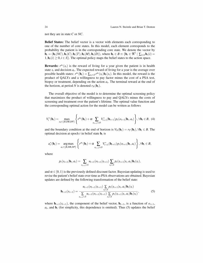
Belief States: The belief vector is a vector with elements each corresponding toone of the number of core states. In this model, each element corresponds to theprobability the patient is in the corresponding core state. We denote the vector bybt = (bt(NC),bt(C),bt(T ),bt(M),bt(D)), where bt ∈ B≡ {bt ∈ℜ5 | ∑i∈S bt(i) =1,bt(i)≥ 0, i ∈ S}. The optimal policy maps the belief states to the action space.

Rewards: rat (st) is the reward of living for a year given the patient is in healthstate st and decision at . The expected reward of living for a year is the average overpossible health states: rat (bt) = ∑st∈S rat (st)bt(st). In this model, the reward is theproduct of QALYs and a willingness to pay factor minus the cost of a PSA test,biopsy or treatment, depending on the action at . The terminal reward at the end ofthe horizon, at period N is denoted rN(bt).

The overall objective of the model is to determine the optimal screening policythat maximizes the product of willingness to pay and QALYs minus the costs ofscreening and treatment over the patient’s lifetime. The optimal value function andthe corresponding optimal action for the model can be written as follows

V ∗t (bt)= maxat∈{B,DB,DP}

{rat (bt)+α ∑

ot+1∈OV ∗t+1(bt+1)pt(ot+1|bt ,at)

},∀bt ∈B, (4)

and the boundary condition at the end of horizon is VN(bt) = rT (bt),∀bt ∈ B. Theoptimal decision at epoch t in belief state bt is

a∗t (bt) = argmaxat∈{B,DB,DP}

{rat (bt)+α ∑

ot+1∈OV ∗t+1(bt+1)pt(ot+1|bt ,at)

},∀bt ∈ B,

where

pt(st+1|bt ,at) = ∑st+1∈S

ut+1(ot+1|st+1) ∑st∈S

pt(st+1|st ,at)bt(st),

and α ∈ [0,1) is the previously defined discount factor. Bayesian updating is used torevise the patient’s belief state over time as PSA observations are obtained. Bayesianupdates are defined by the following transformation of the belief state:

bt+1(st+1) =


pt(st+1|st ,at)bt(st)

∑st+1∈S


pt(st+1|st ,at)bt(st), (5)

where bt+1(st+1), the component of the belief vector, bt+1, is a function of ot+1,at , and bt (for simplicity, this dependence is omitted). Thus (5) updates the belief


state of a patient based on the prior belief state and his most recent observed PSAinterval. The sequence of probabilities {bt , t = 1, · · · ,∞} has been shown to followa Markov process [24], and therefore (4) defines a continuous state MDP.

5.2 Results: Optimal Belief-Based Screening Policy

In this section, we present examples based on the above POMDP model (com-plete details about model parameter estimates and numerical results can be foundin [58]). The data used for parameter estimation in the model consisted of 11,872patients from Olmsted County, Minnesota. It includes PSA values, biopsy informa-tion (if any), diagnosis information (if any), and the corresponding ages for patientsrecorded from 1983 through 2005. This regional data set includes all patients inOlmsted County irrespective of their prostate cancer risk. Prostate cancer probabili-ties conditional on PSA level were estimated from this data set to obtain the informa-tion matrix, Ut . In the results we present, we assume patients detected with prostatecancer were treated by radical prostatectomy. To estimate the annual transition prob-ability from the treatment state, T , to the metastatic cancer state, M, a weighted av-erage of the metastasis rate of three non-metastatic prostate cancer stages based onthe Mayo Clinic Radical Prostatectomy Registry (MCRPR) were used. The diseasespecific transition probability from C to M was based on the metastasis rates re-ported by [61]. The transition probability from state NC to state C was based on theprostate cancer incidence rate estimated from an autopsy review study reported in[62] that provides estimates of prostate cancer prevalence in the general populationin 10-year age intervals. The transition probability from all non-cancer states statesto state D is age specific and was based on the general mortality rate from the Na-tional Vital Statistics Reports [63] minus the prostate cancer mortality rate from the[64]. Note that because the National Cancer Institute reports a single prostate can-cer incidence rate for ages greater than 95 and the National Vital Statistics Reports[63] reports a single all cause mortality rate for ages greater than 95, we assumetransition probabilities were fixed after the age of 95, i.e., N = 95 in the numericalexperiments. The biopsy detection rate was 0.8 based on a study by [59]. To esti-mate the reward function we assumed an annual reward of 1 for each epoch minusdisutilities for biopsy and treatment. Since no estimates of disutility exist yet forprostate biopsy, an estimate based on a bladder cancer study for the occurrence ofsurveillance cystoscopy [65] was used. We assumed patients treated by prostatec-tomy experience disutility due to side effects as reported in [66].

It is well known that POMDPs can be converted into an equivalent completelyobservable MDP on the continuous belief states bt [40]. Even so, as noted earlier,POMDP models are typically much more computationally challenging to solve thancompletely observable MDPs, owing to the continuous nature of the belief statespace. However, due to the low dimensionality of the belief state instances of thisPOMDP, it can be solved exactly incremental pruning [41].


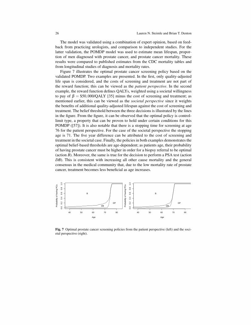
The model was validated using a combination of expert opinion, based on feed-back from practicing urologists, and comparison to independent studies. For thelatter validation, the POMDP model was used to estimate mean lifespan, propor-tion of men diagnosed with prostate cancer, and prostate cancer mortality. Theseresults were compared to published estimates from the CDC mortality tables andfrom longitudinal studies of diagnosis and mortality rates.

Figure 7 illustrates the optimal prostate cancer screening policy based on thevalidated POMDP. Two examples are presented. In the first, only quality-adjustedlife span is considered, and the costs of screening and treatment are not part ofthe reward function; this can be viewed as the patient perspective. In the secondexample, the reward function defines QALYs, weighted using a societal willingnessto pay of β = $50,000/QALY [35] minus the cost of screening and treatment; asmentioned earlier, this can be viewed as the societal perspective since it weightsthe benefits of additional quality-adjusted lifespan against the cost of screening andtreatment. The belief threshold between the three decisions is illustrated by the linesin the figure. From the figure, it can be observed that the optimal policy is control-limit type, a property that can be proven to hold under certain conditions for thisPOMDP ([57]). It is also notable that there is a stopping time for screening at age76 for the patient perspective. For the case of the societal perspective the stoppingage is 71. The five year difference can be attributed to the cost of screening andtreatment in the societal case. Finally, the policies in both examples demonstrates theoptimal belief-based thresholds are age-dependent; as patients age, their probabilityof having prostate cancer must be higher in order for a biopsy referral to be optimal(action B). Moreover, the same is true for the decision to perform a PSA test (actionDB). This is consistent with increasing all other cause mortality and the generalconsensus in the medical community that, due to the low mortality rate of prostatecancer, treatment becomes less beneficial as age increases.

40 50 60 70 80

0.0

0.2

0.4

0.6

0.8

1.0

Age

Pro

babi

lity

of h

avin

g P

Ca

B

DPDB

40 50 60 70 80

0.0

0.2

0.4

0.6

0.8

1.0

Age

Pro

babi

lity

of h

avin

g P

Ca

B

DPDB

Fig. 7 Optimal prostate cancer screening policies from the patient perspective (left) and the soci-etal perspective (right).


6 Open Challenges in MDPs for Chronic Disease

While MDPs serve as a powerful tool for developing screening and treatment poli-cies for chronic diseases, there exist open challenges in terms of formulating theMDPs and implementing the results from MDPs into clinical settings. We reflect onsome of the challenges that were faced in the examples of the previous two sections:

1. Parameter Uncertainty: Many estimates of the parameters used in chronic dis-ease MDPs are subject to error. Transition probabilities among living states areusually estimated from observational data and therefore are subject to samplingerror. Transitions to death states and adverse event states are estimated using riskmodels found in the literature, but usually there is no “gold standard” model.Further, estimates of disutilities due to medications are based on patient surveysand will vary patient-to-patient. As seen in Section 4, MDPs can be sensitiveto changes in the model parameters, which is problematic when the model pa-rameters cannot be known with certainty. For this reason, it will be important todevelop MDP models that are robust in the sense that they perform well undera variety of assumptions of the model parameters, while not being overly con-servative. The reader is referred to [67] and [68] for more about robust dynamicprogramming.

2. State Space Size and Transition Probability Estimates: As discussed in Section 3,the continuously-valued metabolic risk factors are usually discretized to reducethe size of the state space. While a finer discretization of the state space mightbe more representative of the continuous-valued process, this will decrease thesample size of the transitions available for estimating transition probabilities.There is a natural trade-off between the fineness of the discretization of the statespace and the error introduced in the transition probabilities due to sampling.Methods for determining the best discretization of the continuous state-spacewould reduce this barrier to formulating MDPs.

3. Adjusting the Time Frame of Event Probabilities: Many risk models provide theprobability of an event or death within a fixed time (e.g. 10 years). While thisinformation is useful to clinicians, MDP formulation requires converting theselong-term probabilities into transition probabilities between epochs. As men-tioned in Section 4, these probabilities can be converted under the assumptionthat the rate of events is constant, but this may not be realistic in all cases. Deter-mining a method for converting probabilities under different assumptions aboutthe rate of events would improve the accuracy of MDP models that use these riskprobabilities.

4. Solution Methods for a Rapidly Growing State Space: Chronic disease MDPsgrow especially large because of the need to incorporate some history-dependenceinto the state space. Additionally, future models may incorporate risk factors formultiple, coexisting conditions which will cause the state space to grow everlarger. Because MDPs are subject to the curse of dimensionality, these modelscan be computationally-intensive to solve exactly. To provide support to clini-cians in real-time, optimal policies should be able to be solved for quickly. This


will not be possible in many chronic disease models, in which case fast approxi-mation algorithms that provide near-optimal solutions will be necessary.

5. Implementation of Optimal Policies: The goal of these MDPs is to guide screen-ing and treatment decisions made by the clinician. This requires that optimalpolicies can be made easily understood to clinicians. However, if the optimalpolicies are complicated, this could hinder the ability of the clinician to use theMDP results. Therefore, methods for designing structured policies that are near-optimal could potentially improve the likelihood of the policy being implementedin practice.

Tackling these challenges could make MDPs an even more useful tool for guidingclinicians and policy-makers in treatment and screening decisions.

7 Conclusions

Screening and treatment decisions for chronic disease are complicated by the longtime periods over which these decisions are made and the uncertainty in the progres-sion of disease, effects of medication, and correctness of test results. Throughout thischapter, we discussed a number of challenges that arise when modeling these deci-sions using MDPs, such as parameter uncertainty and the rapid growth in the sizeof the state space. Thus, there are still opportunities to study new application areasand develop new methodology, such as robust and approximate dynamic program-ming methods, for solving models in this context. These challenges notwithstand-ing, MDPs have recently found important applications to chronic disease becausethey provide an analytical framework to study the sequential and dynamic decisionsof screening and treating these diseases that develop stochastically over time.

Acknowledgements This material is based in part on work supported by the National ScienceFoundation under grant number CMMI 0969885 (Brian T. Denton). Any opinions, findings, andconclusions or recommendations expressed in this material are those of the authors and do notnecessarily reflect the views of the National Science Foundation.

References

1. M.L. Brandeau, F. Sainfort, and W.P. Pierskalla. Operations Research and Health Care.Kluwer Academic Publishers, Boston, 2004.

2. B.T. Denton. Handbook of Healthcare Operations Management: Methods and Applications.Springer, New York, 2013.

3. G. S. Zaric. Operations Research and Health Care Policy. Springer, 2013.4. O. Alagoz, L. M. Maillart, A. J. Schaefer, and M.S. Roberts. The optimal timing of living

donor liver transplantation. Management Science, 50(10):1420–1430, 2004.5. O. Alagoz, C. L. Bryce, S. M. Shechter, A. J. Schaefer, C.-C. H. Chang, D. C. Angus, and M. S.

Roberts. Incorporating biological natural history in simulation models: Empiric estimates ofthe progression of end-stage liver disease. Medical Decision Making, 25:620–632, 2005.


6. O. Alagoz, L. M. Maillart, A. J. Schaefer, and M. S. Roberts. Which waiting lists should anend-stage liver disease patient join? Technical report, University of Pittsburgh, 2006.

7. O. Alagoz, L.M. Maillart, A.J. Schaefer, and M.S. Roberts. Choosing among living-donor andcadaveric livers. Management Science, 53(11):1702–1715, 2007.

8. D.L. Segev, Gentry S.E., Warren D.S., Reeb B., and R.A. Montgomery. Kidney paired dona-tion and optimizing the use of liver donor organs. Journal of the American Medical Associa-tion, 295:1655–1663, 2005.

9. S.A Zenios, G. M. Chertow, and L.M. Wein. Dynamic allocation of kidneys to candidates onthe trasplant waiting list. Operations Research, 48(4):549–569, 2000.

10. X. Su and S. Zenios. Patient choice in kidney allocation: The role of the queuing discipline.Manufacturing and Service Operations Management, 6(4):280–301, 2005.

11. L.M. Maillart, J.S. Ivy, D. Kathleen, and S. Ransom. Assessing dynamic breast cancer screen-ing policies. Operations Research, 56(6):1411–1427, 2008.

12. J. Chhatwal, O. Alagoz, and E.S. Burnside. Optimal breast biopsy decision-making basedon mammographic features and demographic factors. Operations research, 58(6):1577–1591,2010.

13. E.K. Lee, T. Fox, and I. Crocker. Integer programming applied to intensity-modulated radia-tion therapy treatment planning. Annals of Operations Research, 119:165–181, 2003.

14. A. Holder. Designing radiotherapy plans with elastic constraints and interior point methods.Health Care Management Science, 6:5–16, 2003.

15. F. Preciado-Walters, R. Rardin, M. Langer, and V. Thai. A coupled column generation, mixedinteger approach to optimal planning of intensity modulated radiation therapy for cancer.Mathematical Programming, 101:319–338, 2004.

16. E.K. Lee, R.J. Gallagher, D. Silvern, C. Wu, and M. Zaider. Treatment planning forbrachytherapy: An integer programming model, two computational approaches, and experi-ments with permanent prostate implant planning. Phys. Med. Biol., 44:145–165, 1999.

17. S.M. Shechter, M.D. Bailey, A.J. Schaefer, and M.S. Roberts. The optimal time to initiateHIV therapy under ordered health states. Operations Research, 56(1):20–33, 2008.

18. E.H. Kaplan. Probability models of needle exchange. Operations Research, 43(4):558–569,1995.

19. G. Zaric and M.L. Brandeau. Optimal investment in a portfolio of HIV prevention programs.Medical Decision Making, 21:391–408, 2001.

20. T. Ayer, O. Alagoz, and N.K. Stout. A POMDP approach to personalize mammographyscreening decisions. Operations Research, 60(5):1019–1034, 2012.

21. O. Alagoz, H. Hsu, A. J. Schaefer, and M. S. Roberts. Markov decision processes: A toolfor sequential decision making under uncertainty. Medical Decision Making, 30(4):474–483,2010.

22. A. J. Schaefer, M. D. Bailey, S. M. Shechter, and M. S. Roberts. Modeling medical treatmentusing Markov decision processes. In M. Brandeau, F. Sainfort, and W. Pierskalla, editors,Handbook of Operations Research/Management Science Applications in Health Care, pages597–616. Kluwer Academic Publishers, 2004.

23. E. Regnier and S. M. Shechter. State-space size considerations for disease-progression models.Statistics in medicine, 32(22):3862–3880, 2013.

24. G.E. Monohan. A survey of partially observable Markov decision processes: Theory, models,and algorithms. Management Science, 28(1):1–16, 1982.

25. W. S. Lovejoy. A survey of algorithmic methods for partially observed Markov decisionprocesses. Annals of Operations Research, 28:47–66, 1991.

26. K.A. Anderson, P.M. Odel, P.W.F. Wilson, and W.B. Kannel. Cardiovascular disease riskprofiles. American Heart Journal, 121:293–298, 1991.

27. P.A. Wolf, R.B. D’Agostino, A.J. Belanger, and W.B. Kannel. Probability of stroke: a riskprofile from the Framingham study. Stroke, 22(3):312–318, 1991.

28. P.W.F Wilson, R. B. DAgostino, D. Levy, A. M. Belanger, H. Silbershatz, and W. B. Kannel.Prediction of coronary heart disease using risk factor categories. Circulation, 97(18):1837–1847, 1998.


29. R. C. Turner. The uk prospective diabetes study - a review. Diabetes Care, 21:C35–C38, 1998.30. T.M.E Davis, H. Millns, I.M Stratton, R.R. Holman, and R.C. Turner. Risk factors for stroke in

type 2 diabetes mellitus - United Kingdom Prospective Diabetes Study (UKPDS) 29. Archivesof Internal Medicine, 159(10):1097–1103, 1999.

31. R. J. Stevens, V. Kothari, A. I. Adler, I. M. Stratton, and R. R. Holman. The UKPDS riskengine: a model for the risk of coronary heart disease in type ii diabetes (UKPDS 56). ClinicalScience, 101(6):671–679, 2001.

32. V. Kothari, R.J. Stevens, A. I. Adler, I. M. Stratton, S.E. Manley, H. A. Neil, R. R. Holman,et al. UKPDS 60 risk of stroke in type 2 diabetes estimated by the UK Prospective DiabetesStudy risk engine. Stroke, 33(7):1776–1781, 2002.

33. D.C. Goff, D. M. Lloyd-Jones, G. Bennett, C.J. O’Donnell, S. Coady, and J. Robinson. 2013ACC/AHA guideline on the assessment of cardiovascular risk. J Am Coll Cardiol, 2014.

34. D. Gold, M.R. andStevenson and D.G. Fryback. Halys and qalys and dalys, oh my: Similaritiesand differences in summary measures of population health. Annu. Rev. Public Health, 23:115–134, 2002.

35. K.L. Rascati. The $64,000 question – what is a quality-adjusted life year worth? ClinicalTherapeutics, 28(7):1042–1043, 2006.

36. D.P. Bertsekas and J.N. Tsitsiklis. Neuro-dynamic programming: an overview. In Decisionand Control, 1995., Proceedings of the 34th IEEE Conference on, volume 1, pages 560–564.IEEE, 1995.

37. W.B. Powell. Approximate Dynamic Programming. John Wiley & Sons, Inc, Hoboken, NewJersey, 2007.

38. M.L. Puterman. Markov Decision Processes: Discrete Stochastic Dynamic Programming.John Wiley & Sons, Inc, Hoboken, New Jersey, 1994.

39. M. Kurt, B.T. Denton, A.J. Schaefer, N.D. Shah, and S.A. Smith. The structure of optimalstatin initiation policies for patients with type 2 diabetes. IIE Transaction on HealthcareEngineering, 1:49–65, 2011.

40. R.D. Smallwood and E.J. Sondik. The optimal control of partially observable Markov pro-cesses over a finite horizon. Operations Research, 21(5):1071–1088, 1973.

41. A. Cassandra, M.L. Littman, and N.L. Zhang. Incremental pruning: a simple, fast, exactmethod for partially observable Markov decision processes. Proceedings Thirteenth AnnualConference on Uncertainty in Artificial Intelligence, San Francisco, CA, pages 54–61, 1997.

42. M.L. Littman. The witness algorithm: Solving partially observable Markov decision pro-cesses. Brown University, Providence, RI, 1994.

43. J.E. Eckles. Optimum replacement of stochastically failing systems. Department of ElectricalEngineering, Stanford University., 1966.

44. W.S. Lovejoy. Computationally feasible bounds for partially observed Markov decision pro-cesses. Operations research, 39(1):162–175, 1991.

45. V. Snow, M. D. Aronson, E. R. Hornbake, C. Mottur-Pilson, and K. B. Weiss. Lipid control inthe management of type 2 diabetes mellitus: A clinical practice guideline from the AmericanCollege of Physicians. Annals of Internal Medicine, 140(8):644–649, 2004.

46. D. G. Manuel, K. Kwong, P. Tanuseputro, J. Lim, C. A. Mustard, G. M. Anderson, S. Ardal,D. A. Alter, and A. Laupacis. Effectiveness and efficiency of different guidelines on statintreatment for preventing deaths from coronary heart disease: modelling study. British MedicalJournal, 332(7555):1419–1422, 2006.

47. P.N. Durrington, H. Prais, D. Bhatnagar, M. France, V. Crowley, J. Khan, and J. Morgan. Indi-cations for cholesterol-lowering medication: comparison of risk-assessment methods. Lancet,353(9149):278–281, 1999.

48. B.T. Denton, M. Kurt, N.D. Shah, S.C. Bryant, and S.A. Smith. Optimizing the start time ofstatin therapy for patients with diabetes. Medical Decision Making, 29(3):351–367, 2009.

49. J.E. Mason, D.A. England, B.T. Denton, S.A. Smith, M. Kurt, and N.D. Shah. Optimizingstatin treatment decisions for diabetes patients in the presence of uncertain future adherence.Medical Decision Making, 32(1):154–166, 2012.


50. J.E. Mason, B.T. Denton, N.D. Shah, and S.A. Smith. Optimizing the simultaneous man-agement of blood pressure and cholesterol for type 2 diabetes patients. European Journal ofOperational Research, 233(3):727–738, 2014.

51. S.L. Murphy, J. Xu, and K.D. Kochanek. Deaths: final data for 2010. National vital statisticsreports: from the Centers for Disease Control and Prevention, National Center for HealthStatistics, National Vital Statistics System, 61(4):1–117, 2013.

52. D.K. Miller and S. M. Homan. Determining transition probabilities confusion and suggestions.Medical Decision Making, 14(1):52–58, 1994.

53. M.R. Gold, J.E. Siegel, L.B. Russell, and M.C. Weinstein. Cost-Effectiveness in Health andMedicine. Oxford University Press, New Rork, NY, 1996.

54. O.H. Franco, E. W. Steyerberg, F. B. Hu, J. Mackenbach, and W. Nusselder. Associations ofdiabetes mellitus with total life expectancy and life expectancy with and without cardiovascu-lar disease. Archives of internal medicine, 167(11):1145–1151, 2007.

55. A.V. Chobanian, G. L. Bakris, H. R. Black, W. C. Cushman, L. A. Green, J. L. Izzo Jr, D. W.Jones, B. J. Materson, S. Oparil, J. T. Wright Jr, et al. The seventh report of the Joint NationalCommittee on prevention, detection, evaluation, and treatment of high blood pressure: the JNC7 report. Jama, 289(19):2560–2571, 2003.

56. National Cholesterol Education Program NCEP Expert Panel et al. Third report of the Na-tional Cholesterol Education program (NCEP) expert panel on detection, evaluation, and treat-ment of high blood cholesterol in adults (Adult Treatment Panel III) final report. Circulation,106(25):3143, 2002.

57. J. Zhang, H. Balasubramanian, B.T. Denton, N. Shah, and B. Inman. Optimization of prostatecancer screening decisions: A comparison of patient and societal perspectives. Medical Deci-sion Making, DOI: 10.1177/0272989X11416513, 2011.

58. Jingyu Zhang, Brian T Denton, Hari Balasubramanian, Nilay D Shah, and Brant A Inman.Optimization of prostate biopsy referral decisions. Manufacturing & Service Operations Man-agement, 14(4):529–547, 2012.

59. G.P. Haas, R.F. Delongchamps, V. Jones, V. Chandan, A.M. Seriod, A.J. Vickers, M. Jumbelic,G. Threatte, R. Korets, H. Lilja, and G. De la Roza. Needle biopsies on autopsy prostates:Sensitivity of cancer detection based on true prevalence. Journal of the National CancerInstitute, 99:1484–1849, 2007.

60. R. Gulati, L. Inoue, J. Katcher, W. Hazelton, and R. Etzioni. Calibrating disease progressionmodels using population data: a critical precursor to policy development in cancer control.Biostatistics, 11(4):707–719, 2010.

61. W. J. Catalona, P. T. Scardino, J. R. Beck, B. J. Miles, G. W. Chodak, and R. A. Thisted. Con-servative management of prostate cancer. New England Journal of Medicine, 330(25):1830–1832, 1994.

62. L. Bubendorf, A. Schopfer, U. Wagner, G. Sauter, H. Moch, N. Willi, T. C. Gasser, and M. J.Mihatsch. Metastatic patterns of prostate cancer: an autopsy study of 1,589 patients. Humanpathology, 31(5):578–583, 2000.

63. M. Heron. Deaths: Leading causes for 2004. National Vital Statistics Reports, 56(5):1–96,2007.

64. National Cancer Institute. Surveillance epidemiology and end results.65. Girish S Kulkarni, Shabbir MH Alibhai, Antonio Finelli, Neil E Fleshner, Michael AS Jewett,

Steven R Lopushinsky, and Ahmed M Bayoumi. Cost-effectiveness analysis of immediateradical cystectomy versus intravesical bacillus calmette-guerin therapy for high-risk, high-grade (t1g3) bladder cancer. Cancer, 115(23):5450–5459, 2009.

66. K.E. Bremner, C.A.K.Y. Chong, G. Tomlinson, S.M.H Alibhai, and M.D Krahn. A review andmeta-analysis of prostate cancer utilities. Med Decis Making, 27:288–298, 2007.

67. G.N. Iyengar. Robust dynamic programming. Mathematics of Operations Research,30(2):257–280, 2005.

68. A. Nilim and L.E. Ghaoui. Robust control of Markov decision processes with uncertain tran-sition matrices. Operations Research, 55(5):780–798, 2005.

Documents

Markov Decision Processes for Screening and …btdenton.engin.umich.edu/wp-content/uploads/sites/138/...Markov Decision Processes for Screening and Treatment of Chronic Diseases 3