J Algebr Comb (2014) 40:293–311DOI 10.1007/s10801-013-0488-z

Markov degree of the Birkhoff model

Takashi Yamaguchi · Mitsunori Ogawa ·Akimichi Takemura

Received: 22 April 2013 / Accepted: 14 November 2013 / Published online: 3 December 2013© Springer Science+Business Media New York 2013

Abstract We prove the conjecture by Diaconis and Eriksson (J. Symbolic Comput.41(2):182–195, 2006) that the Markov degree of the Birkhoff model is three. In fact,we prove the conjecture in a generalization of the Birkhoff model, where each voteris asked to rank a fixed number, say r , of candidates among all candidates.

Keywords Algebraic statistics · Markov basis · Normality of semigroup · Rankingmodel

1 Preliminaries

Diaconis and Eriksson [4] conjectured that the Markov degree of the Birkhoff modelis three, i.e., the toric ideal associated with the Birkhoff model is generated by bi-nomials of degree at most three. In this paper we give a proof of this conjecture ina generalization of the Birkhoff model, where each voter is asked to rank a fixednumber of most preferred candidates among all candidates. Our proof is based onarguments of Jacobson and Matthews [6] for Latin squares. The set of Latin squaresis a particular fiber in our setting and our result is also a generalization of [6]. See [1]for terminology of algebraic statistics and toric ideals used in this paper.

Consider an election, where there are n candidates and N voters. Each voter isasked to give r (1 ≤ r ≤ n) preferred candidates and to rank them. For example,

T. Yamaguchi · M. Ogawa (B) · A. TakemuraGraduate School of Information Science and Technology, University of Tokyo, 7-3-1, Hongo,Bunkyo-ku, Tokyo 113-0033, Japane-mail: mitsunori_ogawa@mist.i.u-tokyo.ac.jp

T. Yamaguchie-mail: takashi_yamaguchi@mist.i.u-tokyo.ac.jp

A. Takemurae-mail: takemura@stat.t.u-tokyo.ac.jp

294 J Algebr Comb (2014) 40:293–311

let n = 5, r = 3 and let the candidates be a, b, c, d, e. A vote (a, c, d) by a votermeans that he/she ranks a first, c second and d third. For a positive integer m, denote[m] = {1, . . . ,m}. When the candidates are labeled as 1, . . . , n, the set of possiblevotes is

Sn,r = {σ = (

σ(1), . . . , σ (r)) | σ : injection from [r] to [n]}, |Sn,r | = n!

(n − r)! ,

where σ(j) denotes the candidate chosen in the j th position in the vote σ =(σ (1), . . . , σ (r)). Let ψjk, j ∈ [r], k ∈ [n], be positive parameters and define a prob-ability distribution over Sn,r by

p(σ) = 1

Z

r∏

j=1

ψjσ(j), Z =∑

σ∈Sn,r

r∏

j=1

ψjσ(j). (1)

If ψjk is large, then the candidate k is likely to be ranked in the j th position. Whenr = n, this model is the Birkhoff model [4, 8]. In this paper we call (1) an (n, r)-Birkhoff model. The sufficient statistic of the (n, r)-Birkhoff model consists of num-bers of times the candidate k is ranked in the j th position, j ∈ [r], k ∈ [n]. We denotethe sufficient statistic as (tjk)j∈[r],k∈[n].

Define a 0-1 matrix A = An,r of size rn × (n!/(n − r)!), called a configurationmatrix for the (n, r)-Birkhoff model, whose columns are labeled by σ ∈ Sn,r androws are labeled by (j, k) = (position, candidate), such that the ((j, k), σ )-elementof A is one if and only if σ(j) = k. For example, for n = 4, r = 3, the configurationmatrix A4,3 with labels for its rows and columns is

(123

)(1

24)

(132

)(1

34)

(142

)(1

43)

(213

)(2

14)

(231

)(2

34)

(241

)(2

43)

(312

)(3

14)

(321

)(3

24)

(341

)(3

42)

(412

)(4

13)

(421

)(4

23)

(431

)(4

32)

(1,1) 1 1 1 1 1 1 0 0 0 0 0 0 0 0 0 0 0 0 0 0 0 0 0 0(1,2) 0 0 0 0 0 0 1 1 1 1 1 1 0 0 0 0 0 0 0 0 0 0 0 0(1,3) 0 0 0 0 0 0 0 0 0 0 0 0 1 1 1 1 1 1 0 0 0 0 0 0(1,4) 0 0 0 0 0 0 0 0 0 0 0 0 0 0 0 0 0 0 1 1 1 1 1 1(2,1) 0 0 0 0 0 0 1 1 0 0 0 0 1 1 0 0 0 0 1 1 0 0 0 0(2,2) 1 1 0 0 0 0 0 0 0 0 0 0 0 0 1 1 0 0 0 0 1 1 0 0(2,3) 0 0 1 1 0 0 0 0 1 1 0 0 0 0 0 0 0 0 0 0 0 0 1 1(2,4) 0 0 0 0 1 1 0 0 0 0 1 1 0 0 0 0 1 1 0 0 0 0 0 0(3,1) 0 0 0 0 0 0 0 0 1 0 1 0 0 0 1 0 1 0 0 0 1 0 1 0(3,2) 0 0 1 0 1 0 0 0 0 0 0 0 1 0 0 0 0 1 1 0 0 0 0 1(3,3) 1 0 0 0 0 1 1 0 0 0 0 1 0 0 0 0 0 0 0 1 0 1 0 0(3,4) 0 1 0 1 0 0 0 1 0 1 0 0 0 1 0 1 0 0 0 0 0 0 0 0

(2)

Let x(σ ) ∈ N = {0,1, . . . } be the frequency of voters choosing a vote σ ∈ Sn,r andlet x = {x(σ ) | σ ∈ Sn,r } be the vector of frequencies. Then t = An,rx is the sufficientstatistic vector. For a given t , Ft = {x ∈N

|Sn,r | | Ax = t} is the t -fiber.Let K be any field and let K[{p(σ), σ ∈ Sn,r}] be the polynomial ring in the inde-

terminates p(σ), σ ∈ Sn,r . Similarly let K[{ψjk, j ∈ [r], k ∈ [n]}] be the polynomial

J Algebr Comb (2014) 40:293–311 295

ring in the indeterminates ψjk, j ∈ [r], k ∈ [n]. Let

πn,r : K[{p(σ) | σ ∈ Sn,r

}] → K[{

ψjk, j ∈ [r], k ∈ [n]}]

be a homomorphism defined by

πn,r : p(σ) �→r∏

j=1

ψjσ(j).

Then the toric ideal IA = IAn,r for the (n, r)-Birkhoff model is the kernel of πn,r .Moves for An,r are the elements of the integer kernel kerZ An,r = {z ∈ Z

|Sn,r | | Az =0} of An,r .

Note that if a voter ranks r = n − 1 most preferred candidates, then he/she au-tomatically ranks the last candidate. It is easy to see that the configuration matrixAn,n−1 for the (n,n − 1)-Birkhoff model and the configuration matrix An,n for theBirkhoff model have the same number of columns and their integer kernels are thesame: kerZ An,n−1 = kerZ An,n.

2 Main result and its proof

The main result of this paper is the following theorem.

Theorem 1 For r ≥ 2 and n ≥ 3, the toric ideal IA for the (n, r)-Birkhoff model isgenerated by binomials of degree two and three.

For r = 1 or r = n = 2, the toric ideal IA is trivial. For r ≥ 2 and n ≥ 3, any set ofgenerators for IA contains a binomial of degree three. In the terminology of algebraicstatistics, Theorem 1 states that the Markov degree of the (n, r)-Birkhoff model isthree for r ≥ 2 and n ≥ 3.

The rest of this section is devoted to a proof of this theorem. We define somenotation and terminology for our proof, mainly following [6]. Candidates are denotedeither by letters a, b, c, . . . or by numbers 1, . . . , n. The set of n candidates is denotedby [n], using numbers.

First we give the definition for “valid” votes and definitions for two kinds of “in-valid votes.” Our proof will be based on the idea of swapping candidates between twovotes.

Definition 1 An r ×n integer matrix V = (vjk) is a proper vote if vjk ∈ {0,1},∀j, k,every row sum is one, and every column sum is zero or one. A proper data set of N

votes is the multiset of N proper votes.

Definition 2 An r × n integer matrix V = (vjk) is an improper vote if every rowsum is one, every column sum is zero or one, and there exists a unique cell (j∗, k∗) ∈[r] × [n] such that

vj∗k∗ = −1, vjk ∈ {0,1}, ∀(j, k) = (j∗, k∗).

296 J Algebr Comb (2014) 40:293–311

An improper data set of N votes is the multiset of r × n integer matrices V (1) =(v

(1)jk ), . . . , V (N) = (v

(N)jk ) such that one of them is an improper vote, the others are

proper votes, and∑N

i=1 v(i)jk ≥ 0,∀j, k.

Definition 3 An r × n integer matrix V = (vjk) is a vote with collision if vjk ∈{0,1},∀j, k, every row sum is one and there exists a unique candidate k∗ ∈ [n] suchthat

r∑

j=1

vjk∗ = 2,

r∑

j=1

vjk ∈ {0,1}, ∀k = k∗.

In this case we also say that the vote V contains a collision or the candidate k∗ collidesin V .

Definition 4 An r × n integer matrix V = (vjk) is an improper vote with collision ifevery row sum is one, there exists a unique cell (j∗, k∗) ∈ [r] × [n] such that

vj∗k∗ = −1, vjk ∈ {0,1}, ∀(j, k) = (j∗, k∗),

and there exists a unique candidate k∗∗ ∈ [n] such that

r∑

j=1

vjk∗∗ = 2,

r∑

j=1

vjk ∈ {0,1}, ∀k = k∗∗.

We call a multiset D of r × n integer matrices a data set if each matrix in D is oneof the votes defined in Definitions 1–4.

As in Sect. 1, we often denote votes by row vectors. For proper votes and voteswith collision, we denote them by r-dimensional row vectors whose j th entry is thecandidate ranked in the j th position for each j ∈ [r]. For improper votes we definetheir row vector representation as follows. Let V = (vjk) be an improper vote withvj∗k = vj∗k′ = 1, vj∗k′′ = −1. We denote V by an r-dimensional row vector whosej th entry is the candidate ranked in the j th position for each j ∈ [r] with j = j∗ andthe j∗th entry is k + k′ − k′′. Here, k + k′ − k′′ is just a symbol and we call it animproper element. The following vectors are examples of a proper vote, a vote withcollision and an improper vote, respectively:

(b, a, c, d), (b, a, c, a), (a, d, a, b + c − a).

We also define the row vector representation for improper votes with collision in thesimilar manner.

Several kinds of data sets were defined as the multiset of integer matrices above.For these data sets we use their matrix representation. The matrix representation D

for a data set D = {V (1), . . . , V (N)} is an N × r matrix whose ith row is the rowvector representation of vote V (i) for each i ∈ [N ]. Although the order of the rowsof D is arbitrary, this matrix representation is convenient for our proof. When thereis no confusion, D is also called a data set. Latin squares are also of this form. Theyare tables with N = n = r such that each candidate appears exactly once in each row

J Algebr Comb (2014) 40:293–311 297

and column. An example of improper data set I and its matrix representation I is asfollows:

I =⎧⎨

⎩

⎡

⎣0 0 10 0 11 1 −1

⎤

⎦ ,

⎡

⎣0 1 01 0 00 0 1

⎤

⎦ ,

⎡

⎣1 0 00 1 00 0 1

⎤

⎦

⎫⎬

⎭,

I =⎡

⎣c c a + b − c

b a c

a b c

⎤

⎦ .

In the following, when we display a data set, we mainly use its matrix representation.We now introduce some operations for data sets. Let D = {V (1), . . . , V (N)} be a

data set. Consider a pair of distinct votes in D, say V (i1) = (ν(i1)jk ) and V (i2) = (ν

(i2)jk ).

A swap {i1, i2} : k1j∗↔ k2 for D is an operation transforming D into D′, where

D′ = (D \ {

V (i1), V (i2)}) ∪ {

V (i1), V (i2)}, V (i1) = (

v(i1)jk

), V (i2) = (

v(i2)jk

),

v(i)jk =

⎧⎪⎨

⎪⎩

v(i)jk + 1, (i, j, k) = (i1, j

∗, k2), (i2, j∗, k1),

v(i)jk − 1, (i, j, k) = (i1, j

∗, k1), (i2, j∗, k2),

v(i)jk , otherwise.

In general, D′ is not a data set, because V (i), i = i1, i2, may not be a vote definedabove. If D′ is also a data set, the swap is called an applicable swap. Since only appli-cable swaps appear in our proof, applicable swaps are called merely swaps, hereafter.The swap operation does not alter the sufficient statistic of the data set. Note that theswap may cause a new collision or a new improper element in V (i), i = i1, i2.

The matrix representation of data sets helps intuitive understanding and manipu-lation of the swap operation. The definition of the swap operation shows that the j∗throw of V (i1) is the sum of the j∗th row of V (i1) and a row vector with 0 entries except−1 for the k1th entry and 1 for the k2th entry. Similarly, the j∗th row of V (i2) is thesum of the j∗th row of V (i2) and a row vector with 0 entries except 1 for the k1thentry and −1 for the k2th entry. Hence, the matrix representation D′ of D′ is the sumof the matrix representation D of D and the matrix with 0 entries except k2 − k1 forthe (i1, j

∗)-entry and k1 − k2 for the (i2, j∗)-entry where k2 − k1 and k1 − k2 are

symbols.For illustration, we show an example of swap in the matrix representation of

data sets. Let P = (pij ) be a proper data set in its matrix representation with

p11 = a,p21 = b, a = b and consider a swap {1,2} : a 1↔ b. By adding

[b − a

a − b

]

298 J Algebr Comb (2014) 40:293–311

to the submatrix[ a

b

]we interchange two candidates a and b as

⎡

⎢⎢⎢⎢⎢⎣

a ∗ · · · ∗b ∗ · · · ∗∗ ∗ · · · ∗...

......

...

∗ ∗ · · · ∗

⎤

⎥⎥⎥⎥⎥⎦

+

⎡

⎢⎢⎢⎢⎢⎣

b − a 0 · · · 0a − b 0 · · · 0

0 0 · · · 0...

......

...

0 0 · · · 0

⎤

⎥⎥⎥⎥⎥⎦

=

⎡

⎢⎢⎢⎢⎢⎣

b ∗ · · · ∗a ∗ · · · ∗∗ ∗ · · · ∗...

......

...

∗ ∗ · · · ∗

⎤

⎥⎥⎥⎥⎥⎦

, (3)

where candidates denoted by ∗ are not changed. In this case a and b may collide after

the swap. In order to simplify the notation, we sometimes denote the swap by aj↔ b

or a ↔ b.Let us discuss a sequence of swaps. Consider swapping a and b in two different

positions j, j ′ in the same ith and i′th votes. In our proof below, we often performthese two swaps sequentially, i.e., we swap a and b in the j th position first and thenin the j ′th position. We denote this operation by

aj↔ b

j ′↔ a or

{i, i′

} : a j↔ bj ′↔ a

and call this a double swap. The double swap corresponds to the basic move for no

three-factor interaction model (cf. [2]). As an example, a double swap a1↔ b

2↔ a,where the second swap causes an improper element, is written as

[a b

b c

]+

[b − a a − b

a − b b − a

]=

[b a

a b + c − a

]. (4)

More generally, we consider a sequence of m swaps in positions j1, . . . , jm, suchthat two consecutive swaps involve a common candidate, and denote it as

a1j1↔ a2

j2↔ ·· · jm−1↔ amjm↔ am+1 (5)

or indicating the votes as

{i, i′

} : a1j1↔ a2

j2↔ ·· · jm−1↔ amjm↔ am+1. (6)

We call (5) (or (6)) a chain swap of length m (even when a1 = am+1, i.e., we do notmake a distinction between a chain and a loop). A chain swap of length one is just aswap.

Suppose that we perform several chain swaps for the same two votes and ignorethe order of swaps. An even number of swaps on two proper elements at the sameposition results in no swap and an odd number swaps on two proper elements at thesame position results in a single swap.

On the other hand, we need to be careful for swaps involving an improper element.Let b + c − a be an improper element in the j th position in an improper data set I .Since the elements of the sufficient statistic of I are assumed to be nonnegative, there

J Algebr Comb (2014) 40:293–311 299

is a vote of I containing a in the same position as b+c−a. If we make a swap a ↔ b

between these two elements, then b + c − a becomes c and a becomes b:[b + c − a

a

]+

[a − b

b − a

]=

[c

b

]. (7)

Similarly a ↔ c results in[

bc

]. Note that

[ cb

]and

[bc

]are swaps of each other. Hence

the result of several swaps can be regarded as a single swap a ↔ b or a ↔ c. Althoughthere is an ambiguity between a ↔ b or a ↔ c, the result of a swap between thesevotes at the j th position is either

[bc

]or

[ cb

].

Furthermore we consider a swap between two candidates in(

b+c−ad

), d = a, b, c.

We allow b ↔ d or c ↔ d between these two elements. After b ↔ d we have[b + c − a

d

]→

[d + c − a

b

](8)

and to[

d+c−ab

]we can make further swaps c ↔ b or d ↔ b. The end result of several

swaps is one of the following three cases:

[c + d − a

b

],

[b + d − a

c

]or

[b + c − a

d

].

These three cases correspond to single swaps b ↔ d , c ↔ d and to no swap to[b+c−a

d

].

Although there is an ambiguity on the result of chain swaps involving an improperelement, the end result of several chain swaps is a set of simultaneous swaps of asubset of positions among the two votes. We call this a swap operation for a subsetof positions among two votes, or simply a swap operation among two votes. Whenwe apply a swap operation to a proper or an improper data set D for a subset J ofpositions among two votes R = {i, i′} and the result is D′, we denote the operationby a long double-sided arrow:

DR←→ D′,

where we omit J , because it is often cumbersome to specify J . In this notation wedenote a proper data set by P and an improper data set by I , when we want to clarifythe kinds of data sets, instead of D.

We now give a proof of Theorem 1 in a series of lemmas. Let P and P ′ be twoproper data sets with the same sufficient statistic. Our strategy for a proof is to per-form swap operations to P , involving at most three votes of P at each step, to increasethe number of the common elements in P and P ′. In each operation, elements at thesame position of the three votes of P are permuted. This corresponds to a move ofdegree at most three. In fact, each operation will be further decomposed into a seriesof swap operations among two votes, which involve intermediate improper data sets.

For the ith vote of P and the i′th vote of P ′,

(pi1, . . . , pir ),(p′

i′1, . . . , p′i′r

),

300 J Algebr Comb (2014) 40:293–311

let

C = Ci,i′ = ∣∣{j | pij = p′

i′j}∣∣ (9)

be the number of the same candidates in the same positions in these two votes. Wecall C the number of concurrences. If C = r , then we can remove these two votesfrom P and P ′ and consider other N − 1 votes. On the other hand, we will show thatif C < r , then we can always increase C by a series of swap operations involving atmost three votes of P . The ith vote of P will eventually coincide with the i′th voteof P ′. Then, Theorem 1 is proved by induction on N .

Our first lemma concerns resolving collisions.

Lemma 1 Let D be a data set without any improper element and suppose that atleast one of the ith and i′th votes contains a collision. If each candidate appears atmost twice in these two votes in total, we can resolve all the collisions by a swapoperation among these two votes.

Remark 1 We can prove this lemma based on the normality of the semigroup gener-ated by the configuration matrix An,r such as A4,3 in (2). The normality follows fromresults in [7, 9] and [3]. We will discuss this point again in Sect. 3.2. However, wegive our own proof of Lemma 1, because we will use similar arguments for improperdata sets. Arguments based on the normality cannot be applied to improper data sets.

Proof We may assume i = 1 and i′ = 2 and at least the first vote contains a collision.We first consider the case that there is only one collision in the two votes. Let a denotethe colliding candidate. Relabeling the positions, without loss of generality, the twovotes are displayed as

[a a d ∗ · · · ∗b c ∗ ∗ · · · ∗

],

where b = c. We choose one of the two a’s arbitrarily, say in the second position, and

make a swap a2↔ c with the following result:

[a c d ∗ . . . ∗b a ∗ ∗ · · · ∗

]. (10)

Since a appears at most twice in these two votes in total, a does not collide in thesecond vote. However, c might again collide in the first vote, e.g.,

[a c d c ∗ . . . ∗ ]

.

We then make a swap for c, which was in the first vote from the beginning (in this

example c4↔ ∗). If we continue this process, we always have collisions in the first

vote. If this process ends in finite number of steps, then by a chain swap we resolvethe collisions of a and subsequent collisions due to swaps. We claim that this processindeed ends in finite number of steps. Actually we show a stronger result that nocandidate appears twice in this process of resolving collisions.

J Algebr Comb (2014) 40:293–311 301

Suppose otherwise. Then there is a candidate, say α, which is swapped twice forthe first time. We consider two cases: α = a and α = a.

Consider the case α = a. The process of swaps is displayed as follows:

a ↔ c ↔ s1 ↔ ·· · ↔ sl−1 ↔ a ↔ ·· · .

Since the collision always occurs in the first vote, the candidate a was moved fromthe second vote to the first vote in the swap sl−1 ↔ a. By (10) we have c = sl−1,which contradicts the assumption that α = a is the first candidate colliding twice.

Consider the case α = a. The process of swaps is displayed as follows:

a ↔ c ↔ s1 ↔ ·· · ↔ sl−1 ↔ α ↔ sl+1 ↔ ·· · ↔ sm−1 ↔ α ↔ ·· · . (11)

Considering the subprocess of (11) which starts from the first α, we can apply thediscussion for the α = a and confirm that there exists a contradiction. We have shownthe lemma for the case that there is only one collision.

Now suppose that there are m colliding candidates a1, a2, . . . , am. Each of thesecandidates appears in one of the votes twice. Temporarily, we assign different labels,say a′

l , a′′l , l = 2, . . . ,m, to candidates except for a1, namely, we ignore collisions of

a2, . . . , am. By the above procedure we resolve the collision of a1 and subsequentcollisions. When this procedure is finished, we restore the labels a′

l , a′′l → al , l =

2, . . . ,m. Then some collisions of a2, . . . , am may have been already resolved, butwe do not have any new collision. Hence, by the above procedure we decrease thenumber of collisions. As long as there is a remaining collision, we can repeat thisprocedure and resolve all the collisions. �

So far we discussed resolving collisions. We now consider resolving an improperelement by a swap operation among two votes.

Lemma 2 Let I be an improper data set containing an element b + c − a. By a swapoperation among two votes, I can be transformed to a proper data set.

Proof Without loss of generality, assume that the first vote contains b + c − a andthe second vote contains a. We can then make a swap {1,2} : a ↔ b, as in (7). Herea may collide in the first vote and b may collide in the second vote. However, botha and b appear at most twice in these two votes. Hence we can now resolve thesepossible collisions by Lemma 1 by a swap operation among these two votes. �

The operation of Lemma 2 is denoted by

IR←→ P, (12)

where R is a set of two votes of I .At this point we make the following two definitions.

Definition 5 We call two votes in Lemma 2 of the form

iimipr

[∗ · · · ∗ b + c − a ∗ · · · ∗∗ · · · ∗ a ∗ · · · ∗

]

302 J Algebr Comb (2014) 40:293–311

a resolvable pair. Here iim is an improper vote and ipr is a proper vote. A resolvablepair is denoted as [iim, ipr].

Note that any improper data set I contains a resolvable pair [iim, ipr] and R in (12) isthe set of votes of a resolvable pair.

Definition 6 A swap operation among two votes R = {i, i′} in IR←→ I ′ is compati-

ble with improper data sets I and I ′ if there exists a common resolvable pair [iim, ipr]of I and I ′ such that R ∩ {iim, ipr} = ∅, or equivalently |R ∪ {iim, ipr}| ≤ 3.

Lemma 3 Let P,P ′ be two proper data sets with the same sufficient statistic. Sup-pose that the ith vote of P and the i′th vote of P ′ are different, i.e., V (i) = V ′(i′),and let C < r in (9) be the number of concurrences in these two votes. Then, C canbe increased by at most three steps of swap operations among two votes of P , where(1) each intermediate swap operation between two consecutive improper data sets iscompatible with them, and (2) if the resulting data set is improper then its impropervote and the ith vote form a resolvable pair.

Proof Without loss of generality we consider the first votes of P and P ′. We considertwo disjoint cases.

Case 1 The same candidate appears in distinct positions in the two votes.Let b be the candidate appearing in the distinct positions in the two votes.

Relabeling the positions, without loss of generality, let p11 = a, p′11 = b, a = b,

and p12 = b. Since P ′ contains b in the first position and the sufficient statistic ofP and P ′ are the same, P has to contain b in the first position, say p21 = b. We

now perform a double swap a1↔ b

2↔ a to P :

⎡

⎢⎢⎢⎢⎢⎣

a b ∗ · · · ∗b c ∗ · · · ∗∗ ∗ ∗ · · · ∗...

......

......

∗ ∗ ∗ · · · ∗

⎤

⎥⎥⎥⎥⎥⎦

→

⎡

⎢⎢⎢⎢⎢⎣

b a ∗ · · · ∗a b + c − a ∗ · · · ∗∗ ∗ ∗ · · · ∗...

......

......

∗ ∗ ∗ · · · ∗

⎤

⎥⎥⎥⎥⎥⎦

,

where ∗’s are not changed. By this double swap C is increased. If c = a, the swapresults in a proper data set. Otherwise, the swap results in an improper data set,where [2,1] forms a resolvable pair. Therefore, C is increased by a process of the

form P{1,2}←→ P or P

{1,2}←→ I .Case 2 Every candidate appearing twice in the two votes appears in the same posi-

tion.Again, let p11 = a, p′

11 = b, a = b. The candidate b does not appear in thefirst vote of P and a does not appear in the first vote of P ′. As in Case 1, we canassume p21 = b. Since the first vote of P ′ does not contain a, the total frequencyof the candidate a in P ′ is less than N . Since the sufficient statistic is common, itfollows that there is a vote of P which does not contain a.

J Algebr Comb (2014) 40:293–311 303

If the second vote does not contain a, we can make a swap a1↔ b among the

first two votes and increase C without causing collision. This process is of the

form P{1,2}←→ P .

If the second vote contains a, without loss of generality, let p22 = a and alsoassume that the third vote of P does not contain a. Let p32 = c = a. Since a ischosen in the second vote and not chosen in the third vote and both votes have thesame number r of candidates, there is a candidate d , who is chosen in the thirdvote but is not chosen in the second vote. If d is in the position j > 2, then byrelabeling of positions we assume that p33 = d . Then P looks like

⎡

⎢⎢⎢⎢⎢⎢⎢⎣

a ∗ ∗ · · · ∗b a ∗ · · · ∗d c ∗ · · · ∗∗ ∗ ∗ · · · ∗...

...... · · · ...

∗ ∗ ∗ · · · ∗

⎤

⎥⎥⎥⎥⎥⎥⎥⎦

or

⎡

⎢⎢⎢⎢⎢⎢⎢⎣

a ∗ ∗ · · · ∗b a ∗ · · · ∗∗ d(= c) ∗ · · · ∗∗ ∗ ∗ · · · ∗...

...... · · · ...

∗ ∗ ∗ · · · ∗

⎤

⎥⎥⎥⎥⎥⎥⎥⎦

or

⎡

⎢⎢⎢⎢⎢⎢⎢⎣

a ∗ ∗ · · · ∗b a ∗ · · · ∗∗ c d · · · ∗∗ ∗ ∗ · · · ∗...

...... · · · ...

∗ ∗ ∗ · · · ∗

⎤

⎥⎥⎥⎥⎥⎥⎥⎦

.

We perform a swap {2,3} : a2↔ d to the second position of the second and third

votes:⎡

⎢⎢⎢⎢⎢⎢⎢⎣

a ∗ ∗ · · · ∗b d ∗ · · · ∗d a + c − d ∗ · · · ∗∗ ∗ ∗ · · · ∗...

...... · · · ...

∗ ∗ ∗ · · · ∗

⎤

⎥⎥⎥⎥⎥⎥⎥⎦

or

⎡

⎢⎢⎢⎢⎢⎢⎢⎣

a ∗ ∗ · · · ∗b d ∗ · · · ∗∗ a ∗ · · · ∗∗ ∗ ∗ · · · ∗...

...... · · · ...

∗ ∗ ∗ · · · ∗

⎤

⎥⎥⎥⎥⎥⎥⎥⎦

or

⎡

⎢⎢⎢⎢⎢⎢⎢⎣

a ∗ ∗ · · · ∗b d ∗ · · · ∗∗ a + c − d d · · · ∗∗ ∗ ∗ · · · ∗...

...... · · · ...

∗ ∗ ∗ · · · ∗

⎤

⎥⎥⎥⎥⎥⎥⎥⎦

.

After the swap the second vote does not contain a. The result is proper if c = d

(the middle case) and improper if c = d .

Now we apply a swap {1,2} : a1↔ b for the first position of the first and the

second votes and increase V . In the case c = d , the last swap was performed on

304 J Algebr Comb (2014) 40:293–311

an improper data set, but it is compatible with the data sets. Furthermore we canresolve the improper element a + c − d by Lemma 2, since [3,2] is a resolvable

pair. The process in this case is summarized as P{2,3}←→ P

{1,2}←→ P or P{2,3}←→

I{1,2}←→ I

{2,3}←→ P .

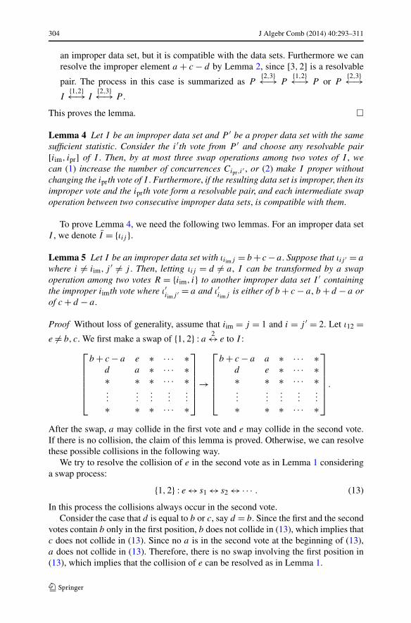
This proves the lemma. �

Lemma 4 Let I be an improper data set and P ′ be a proper data set with the samesufficient statistic. Consider the i′th vote from P ′ and choose any resolvable pair[iim, ipr] of I . Then, by at most three swap operations among two votes of I , wecan (1) increase the number of concurrences Cipr,i′ , or (2) make I proper withoutchanging the iprth vote of I . Furthermore, if the resulting data set is improper, then itsimproper vote and the iprth vote form a resolvable pair, and each intermediate swapoperation between two consecutive improper data sets, is compatible with them.

To prove Lemma 4, we need the following two lemmas. For an improper data setI , we denote I = {ιij }.

Lemma 5 Let I be an improper data set with ιiimj = b + c − a. Suppose that ιij ′ = a

where i = iim, j ′ = j . Then, letting ιij = d = a, I can be transformed by a swapoperation among two votes R = {iim, i} to another improper data set I ′ containingthe improper iimth vote where ι′

iimj ′ = a and ι′iimj is either of b + c − a, b + d − a orof c + d − a.

Proof Without loss of generality, assume that iim = j = 1 and i = j ′ = 2. Let ι12 =e = b, c. We first make a swap of {1,2} : a 2↔ e to I :

⎡

⎢⎢⎢⎢⎢⎣

b + c − a e ∗ · · · ∗d a ∗ · · · ∗∗ ∗ ∗ · · · ∗...

......

......

∗ ∗ ∗ · · · ∗

⎤

⎥⎥⎥⎥⎥⎦

→

⎡

⎢⎢⎢⎢⎢⎣

b + c − a a ∗ · · · ∗d e ∗ · · · ∗∗ ∗ ∗ · · · ∗...

......

......

∗ ∗ ∗ · · · ∗

⎤

⎥⎥⎥⎥⎥⎦

.

After the swap, a may collide in the first vote and e may collide in the second vote.If there is no collision, the claim of this lemma is proved. Otherwise, we can resolvethese possible collisions in the following way.

We try to resolve the collision of e in the second vote as in Lemma 1 consideringa swap process:

{1,2} : e ↔ s1 ↔ s2 ↔ ·· · . (13)

In this process the collisions always occur in the second vote.Consider the case that d is equal to b or c, say d = b. Since the first and the second

votes contain b only in the first position, b does not collide in (13), which implies thatc does not collide in (13). Since no a is in the second vote at the beginning of (13),a does not collide in (13). Therefore, there is no swap involving the first position in(13), which implies that the collision of e can be resolved as in Lemma 1.

J Algebr Comb (2014) 40:293–311 305

Consider the case d = b, c. The difference of this case from Lemma 1 is that theprocess (13) may hit the first position. This happens when d appears in (13) for the

fist time as slj↔ d , j = 1, and d = ι1j in the first vote is swapped down to the second

vote in the j th position. Then we need to choose b or c and make the swap d ↔ b

or d ↔ c in the first position. By symmetry, without loss of generality, we perform

d1↔ c:

[b + c − a

d

]→

[b + d − a

c

].

This amounts to ignoring b and −a and we look at the improper element b + c − a

just as a proper element c in resolving the collision of e. We leave b − a in the (1,1)-element of I as it is during the sequence in (13). Then just as in Lemma 1 it followsthat no candidate appears twice in (13). Note that b and −a which were left in the(1,1)-element cause no trouble, because collision occurs always in the second vote.Indeed, b causes no trouble because it does not leave the first vote. The candidate a

causes no trouble because the second vote does not initially contain a and when a isswapped from the first vote to the second vote, then the process in (13) ends at thatpoint.

After the collision of e is resolved, a may still collide in the first vote. Let j1 andj2, j1 = j2, be the labels of positions containing a in the first vote other than the firstposition. To resolve this collision we consider the following two swap processes:

{1,2} : a j1↔ s1 ↔ s2 ↔ ·· · , (14)

{1,2} : a j2↔ s′1 ↔ s′

2 ↔ ·· · , (15)

where no swap in the j2th position is involved in (14) and no swap in the j1th po-sition is involved in (15). Since every candidate in the first and second votes excepta appears in at most two positions, the common candidate involved both in (14) andin (15) is a only. Then one of (14) and (15), say (14), involves neither b nor c, orinvolves b and no c. Therefore, ignoring c,−a and a in the j2th column, we see thatthe swap process (14) ends in finite number of steps as in Lemma 1. �

Lemma 6 Let I be an improper data set with an improper element ιiimj = b + c −a. Let ιij = d, i = iim, and suppose that d = a, b, c. Then I can be transformed toanother improper data set I ′ by a swap operation among two votes R = {iim, i} suchthat either ι′iimj = b + d − a, ι′ij = c or ι′iimj = c + d − a, ι′ij = b.

Proof Without loss of generality assume iim = j = 1 and i = 2. Then the upper-left2 × 1 submatrix of I is

[b+c−a

d

]. Note that [1,2] is not a resolvable pair because

d = a.

We begin by considering two swaps of {1,2} : d 1↔ b and {1,2} : d 1↔ c. If {1,2} :d

1↔ b is applied to I , b may collide in the second vote and d may collide in the

first vote. If {1,2} : d1↔ c is applied to I , c may collide in the second vote and d

306 J Algebr Comb (2014) 40:293–311

may collide in the first vote. Considering the resolution of possible collisions in thesecond vote for each swap, the following two swap processes are obtained:

{1,2} : d 1↔ b ↔ s1 ↔ s2 ↔ ·· · , (16)

{1,2} : d 1↔ c ↔ s′1 ↔ s′

2 ↔ ·· · . (17)

Since the number of positions which contains a in the first or second vote is at mostthree, one of (16) and (17), say (16), contains a at most once. Note that each candi-dates other than a appears in the first and second votes at most twice. If (16) doesnot contain a, we see that (16) ends in finite number of steps as in Lemma 1. If (16)contains one a, the finiteness of (16) is proved by applying the similar discussion ofLemma 1 for the subprocess of (16) which starts from a.

After resolving the collision of b in the second vote, d may still collide in the firstvote. At this point the second vote contains at most one a. Consider a swap process

{1,2} : d ↔ s′′1 ↔ s′′

2 ↔ ·· · . (18)

Since b has already been involved in (16), no s′′i is equal to b. If some s′′

i is c, thechain swap

{1,2} : d ↔ s′′1 ↔ s′′

2 ↔ ·· · ↔ c

resolves the collisions in the first vote. Since a appears in the second vote at mostonce, the process (18) contains a at most once. If a does not appear in (18), theprocess does not hit the first position and we see that (16) ends in finite number ofsteps as in Lemma 1. If a appears in (18), the finiteness of (16) is proved by applyingthe similar discussion of Lemma 1 for the subprocess of (16) which starts from a. �

Using Lemmas 5 and 6 we shall prove Lemma 4.

Proof of Lemma 4 Without loss of generality, let i′ = 1, [iim, ipr] = [2,1], ι11 = a,and ι21 = b + c − a. Then I looks like

⎡

⎢⎢⎢⎢⎢⎣

a ∗ · · · ∗b + c − a ∗ · · · ∗

∗ ∗ · · · ∗...

......

...

∗ ∗ · · · ∗

⎤

⎥⎥⎥⎥⎥⎦

.

In the cases below, where a resulting data set is improper, [2,1] will be a resolvablepair.

Case 1 p′11 = a.

In this case in P ′ and hence in I , the candidate a appears at least once in the firstposition. Therefore a is in the first position in some vote i > 2 in I . Let i = 3. Thenthe votes [2,3] of I form a resolvable pair and I can be transformed to a properdata set by Lemma 2. This corresponds to (2) of the lemma and is summarized as

I{2,3}←→ P .

J Algebr Comb (2014) 40:293–311 307

Case 2 p′11 = a, but a appears in the first vote of P ′.

Without loss of generality let p′12 = a. Let d = ι12.

Case 2-1 ι22 = a.

We perform the double swap a1↔ d

2↔ a to the first two votes

⎡

⎢⎢⎢⎢⎢⎣

a d ∗ · · · ∗b + c − a a ∗ · · · ∗

∗ ∗ ∗ · · · ∗...

......

......

∗ ∗ ∗ · · · ∗

⎤

⎥⎥⎥⎥⎥⎦

→

⎡

⎢⎢⎢⎢⎢⎣

d a ∗ · · · ∗b + c − d d ∗ · · · ∗

∗ ∗ ∗ · · · ∗...

......

......

∗ ∗ ∗ · · · ∗

⎤

⎥⎥⎥⎥⎥⎦

.

This increases C11. This corresponds to (1) of the lemma and is summarized as

I{1,2}←→ I .

Case 2-2 ι22 = a.Since p′

12 = a, a has to appear in the second position of I . Without loss of gener-ality, let ι32 = a. Let e = ι31 and f = ι22. Then P looks like

⎡

⎢⎢⎢⎢⎢⎢⎢⎣

a d ∗ · · · ∗b + c − a f ∗ · · · ∗

e a ∗ · · · ∗∗ ∗ ∗ · · · ∗...

......

......

∗ ∗ ∗ · · · ∗

⎤

⎥⎥⎥⎥⎥⎥⎥⎦

.

From Lemma 5 applied to votes {2,3}, this case is reduced to Case 2-1. This

case together with the subsequent operation of Case 2-1 is summarized as I{2,3}←→

I{1,2}←→ I .

Case 3 a does not appear in the first vote of P ′.Let d = p′

11, d = a. If d = b or d = c, we directly go to the Cases 3-1 or Case 3-2below. If d = b, c, we need an extra step as follows. Let ι31 = d without loss ofgenerality. Then I looks like

⎡

⎢⎢⎢⎢⎢⎢⎢⎣

a ∗ · · · ∗b + c − a ∗ · · · ∗

d ∗ · · · ∗∗ ∗ · · · ∗...

......

...

∗ ∗ · · · ∗

⎤

⎥⎥⎥⎥⎥⎥⎥⎦

.

By Lemma 6 applied to votes {2,3}, we move d to the second vote resolving thepossible collisions. At this point the (2,1)-element of I may be b + d − a or c +

308 J Algebr Comb (2014) 40:293–311

d − a. We consider the former case without loss of generality. Then I looks like

⎡

⎢⎢⎢⎢⎢⎢⎢⎣

a ∗ · · · ∗b + d − a ∗ · · · ∗

c ∗ · · · ∗∗ ∗ · · · ∗...

......

...

∗ ∗ · · · ∗

⎤

⎥⎥⎥⎥⎥⎥⎥⎦

. (19)

Case 3-1 d appears in the first vote of I .

Let d = ι12 without loss of generality. We apply a double swap a1↔ d

2↔ a:

⎡

⎢⎢⎢⎢⎢⎣

a d ∗ · · · ∗b + d − a e ∗ · · · ∗

∗ ∗ ∗ · · · ∗...

......

......

∗ ∗ ∗ · · · ∗

⎤

⎥⎥⎥⎥⎥⎦

→

⎡

⎢⎢⎢⎢⎢⎣

d a ∗ · · · ∗b d + e − a ∗ · · · ∗∗ ∗ ∗ · · · ∗...

......

......

∗ ∗ ∗ · · · ∗

⎤

⎥⎥⎥⎥⎥⎦

.

This case is summarized as I{1,2}←→ I or I

{2,3}←→ I{1,2}←→ I , where I

{2,3}←→ I is neededfor the case d = b, c. We do not repeat this comment for the other cases below.

Case 3-2 d does not appear in the first vote of I .If a appears only once in the second vote, say in the j th position, j > 1, then

we can apply the swap {1,2} : a1↔ d to make I proper, which is summarized as

I{1,2}←→ P or I

{2,3}←→ I{1,2}←→ P .

Hence we consider the case that a appears in two positions labeled by j1, j2, 1 <

j1 < j2 of the second vote of I . Since P ′ does not contain a in the first vote, I hasa vote not containing a.

Case 3-2-1 The third vote of (19) contains a.Without loss of generality, suppose the fourth vote of I does not contain a. Denotee = ι41. Interpreting two a’s in the second vote as a collision, we try to resolvethe collision by swapping a down to the fourth vote. Then we have two processesof swaps

{2,4} : a j1↔ s1 ↔ s2 ↔ ·· · , (20)

{2,4} : a j2↔ s′1 ↔ s′

2 ↔ ·· · . (21)

During these processes the collisions occur in the second vote. Only one of thesetwo can contain d . Then we can choose a process, say (20), which does not con-tain d . As in Lemma 1 no candidate appears twice in (20). Hence, (20) is a finitechain swap resolving the collisions.

J Algebr Comb (2014) 40:293–311 309

At this stage I looks like

⎡

⎢⎢⎢⎢⎢⎢⎢⎢⎢⎣

a ∗ · · · ∗b + d − a ∗ · · · ∗

c ∗ · · · ∗e ∗ · · · ∗∗ ∗ · · · ∗...

......

...

∗ ∗ · · · ∗

⎤

⎥⎥⎥⎥⎥⎥⎥⎥⎥⎦

or

⎡

⎢⎢⎢⎢⎢⎢⎢⎢⎢⎣

a ∗ · · · ∗e + d − a ∗ · · · ∗

c ∗ · · · ∗b ∗ · · · ∗∗ ∗ · · · ∗...

......

...

∗ ∗ · · · ∗

⎤

⎥⎥⎥⎥⎥⎥⎥⎥⎥⎦

.

In either case, the swap {1,2} : a 1↔ d increases C and makes I proper. The whole

process for this case is summarized as I{2,4}←→ I

{1,2}←→ P or I{2,3}←→ I

{2,4}←→ I{1,2}←→

P .Case 3-2-2 The third vote of (19) does not contain a.We can just use the third vote of (19) as the fourth vote of the previous case. Hence

I{2,4}←→ I is replaced by I

{2,3}←→ I and this case is summarized as I{2,3}←→ I

{1,2}←→ P .�

We now summarize what we have proved so far. We will again discuss the follow-ing result in Sect. 3.1.

Let P and P ′ be two proper data sets with the same sufficient statistic, respectively.Suppose that the ith vote of P and the i′th vote of P ′ are different, i.e., V (i) = V (i′).If we allow improper data sets, then by a sequence of swap operations among twovotes of P , we can make the ith vote of P identical with the i′th vote of P ′. Thenwe throw away this common vote from the two data sets and repeat the procedure. Itshould be noted that P may have been transformed to an improper data set I whentwo votes coincide, but I contains a resolvable pair [iim, ipr] with ipr = i. Hence wecan continue this process until P is fully transformed to P ′.

In order to finish our proof of Theorem 1, we have to show that each interme-diate improper data set can be temporarily transformed to a proper data set and theconsecutive proper data sets are connected by operations among three votes.

We decompose the whole process of transforming P to P ′ into segments thatconsist of transformations from a proper data set to another proper data set withimproper intermediate steps. One segment is depicted as follows:

P1 ←→ I1 ←→ ·· · ←→ Ii ←→ Ii+1 ←→ ·· · ←→ Im ←→ Pm, (22)

where each ←→ (omitting R) denotes a swap operation among two votes in Lem-mas 3 and 4. By these lemmas, the number of concurrences in Pm is larger than inP1. We claim that for any consecutive improper data sets Ii , Ii+1, we can find properdata sets Pi,P

′i , P

′i+1 satisfying

Pi ←→ Ii ←→ Ii+1 ←→ P ′i+1, (23)

P ′i ←→ Ii ←→ Pi. (24)

310 J Algebr Comb (2014) 40:293–311

The swap operation for Ii ←→ Ii+1 is compatible with both data sets. Hence if wechoose a common resolvable pair for Ii and Ii+1, then (23) for transforming Pi to P ′

i

involves three votes. On the other hand, since both P ′i ←→ Ii and Ii ←→ Pi involve

an improper vote, the operation of transforming P ′i to Pi involves three votes. This

completes the proof of Theorem 1.

3 Discussion

In this section we discuss some topics related to our main result.

3.1 Extension of fibers by allowing one negative element

As discussed after the proof of Lemma 4, we have shown the following result by ourproof of Theorem 1 (cf. (22)).

Proposition 1 Let P and P ′ be any two proper data sets with the same sufficientstatistic. If we allow improper data sets as the intermediate states, P and P ′ areconnected by swap operations among two votes, whose single operation is used ateach step.

Since an improper data set has one −1, Proposition 1 seems to suggest that everyfiber Ft for the configuration An,r becomes connected by degree two moves if weextend Ft by allowing one negative element x(σ ) = −1 in x which satisfies t = Ax.However, this is incorrect. In fact, allowing −1 in data set and allowing −1 in Ft aretwo different things.

For example, consider the case of n = 3 and r = 2 with candidates labeled asa, b, c. It is easy to see that dim kerA3,2 = 1 and IA3,2 is a principal ideal generatedby a single binomial p(ab)p(bc)p(ca)−p(ac)p(cb)p(ba). Hence there is no degreetwo move in kerZ A3,2. Yet, we can connect two data sets

P =⎡

⎣a b

b c

c a

⎤

⎦ , P ′ =⎡

⎣a c

c b

b a

⎤

⎦

by applying {2,3} : a 1↔ b, {1,2} : b 2↔ c and {2,3} : a 1↔ c in this order:⎡

⎣a b

b c

c a

⎤

⎦ →⎡

⎣a b

a c

b + c − a a

⎤

⎦ →⎡

⎣a c

a b

b + c − a a

⎤

⎦ →⎡

⎣a c

c b

b a

⎤

⎦ .

Note that the middle two data sets can be interpreted either as

adding (ab), (ac), (bc), (ca) and subtracting (ac)

or as

adding (ab), (ac), (ba), (cb) and subtracting (ab).

However the middle two data sets do not correspond to an element of a fiber for A3,2.

J Algebr Comb (2014) 40:293–311 311

3.2 Normality

It is natural to ask if the semigroup generated by An,r is normal. Consider the set Q

of n × r real matrices X = {xij } satisfying

0 ≤ xij ≤ 1, ∀i, j,

r∑

j=1

xij ≤ 1,∀i,

n∑

i=1

xij = 1,∀j.

The set Q is the Birkhoff polytope in Rn×r , which is a special case of transportation

polytopes [5]. By [3] the set of vertices of Q is exactly the same as the set of columnsof An,r . Then by the results of [7] and [9] the semigroup generated by An,r is normal.Lemma 1 is a consequence of this normality, because by the normality there exist twovalid votes with the same sufficient statistic as the ith and the i′th votes in Lemma 1.These two proper votes can be obtained from the two votes of a swap operation inLemma 1. However, the normality is not useful in proving Lemmas 5 and 6.

3.3 Generation of moves for running a Markov chain

Based on Theorem 1 we can run a Markov chain for general r as follows. We ran-domly generate two or three proper votes of r candidates out of n candidates. Oncethese votes are obtained, we randomly perform permutations of candidates in thesame position. We do this for each position. If no collision occurs, then we have twoor three proper votes. If the obtained set of votes is different from the initial set, thenthe difference is a move. In this way, we obtain a random move of degree two or threeand then run a Markov chain over a given fiber. Extensive computational results onMarkov bases of (n, r)-Birkhoff models for r ≤ 5 and arbitrary n are available fromthe authors.

Acknowledgements This work is partially supported by Grant-in-Aid for JSPS Fellows (No. 12J07561)from Japan Society for the Promotion of Science (JSPS). The authors thank the anonymous referees fortheir valuable comments.

References

1. Aoki, S., Hara, H., Takemura, A.: Markov Bases in Algebraic Statistics. Springer Series in Statistics.Springer, New York (2012)

2. Aoki, S., Takemura, A.: Minimal basis for a connected Markov chain over 3 × 3 × K contingencytables with fixed two-dimensional marginals. Aust. N. Z. J. Stat. 45(2), 229–249 (2003)

3. Brualdi, R.A., Dahl, G.: An extension of the polytope of doubly stochastic matrices. Linear MultilinearAlgebra 61(3), 393–408 (2013)

4. Diaconis, P., Eriksson, N.: Markov bases for noncommutative Fourier analysis of ranked data. J. Symb.Comput. 41(2), 182–195 (2006)

5. Haase, C., Paffenholz, A.: Quadratic Gröbner bases for smooth 3 × 3 transportation polytopes. J. Al-gebr. Comb. 30(4), 477–489 (2009)

6. Jacobson, M.T., Matthews, P.: Generating uniformly distributed random Latin squares. J. Comb. Des.4(6), 405–437 (1996)

7. Ohsugi, H., Hibi, T.: Convex polytopes all of whose reverse lexicographic initial ideals are squarefree.Proc. Am. Math. Soc. 129(9), 2541–2546 (2001) (electronic)

8. Sturmfels, B., Welker, V.: Commutative algebra of statistical ranking. J. Algebra 361, 264–286 (2012)9. Sullivant, S.: Compressed polytopes and statistical disclosure limitation. Tohoku Math. J. 58(3), 433–

445 (2006)