Markov Random Fields for

Computer Vision (Part 1)Machine Learning Summer School (MLSS 2011)

Stephen Gouldstephen.gould@anu.edu.au

Australian National University

13–17 June, 2011

Stephen Gould 1/23

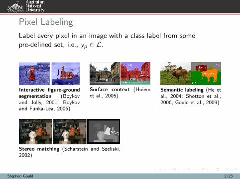
Pixel Labeling

Label every pixel in an image with a class label from somepre-defined set, i.e., yp ∈ L.

Stephen Gould 2/23

Pixel Labeling

Label every pixel in an image with a class label from somepre-defined set, i.e., yp ∈ L.

Interactive figure-groundsegmentation (Boykovand Jolly, 2001; Boykovand Funka-Lea, 2006)

Stephen Gould 2/23

Pixel Labeling

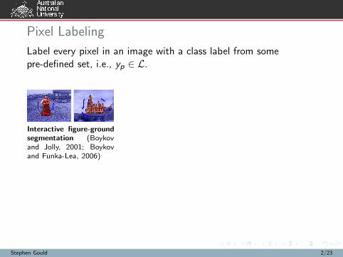
Label every pixel in an image with a class label from somepre-defined set, i.e., yp ∈ L.

Interactive figure-groundsegmentation (Boykovand Jolly, 2001; Boykovand Funka-Lea, 2006)

Surface context (Hoiemet al., 2005)

Stephen Gould 2/23

Pixel Labeling

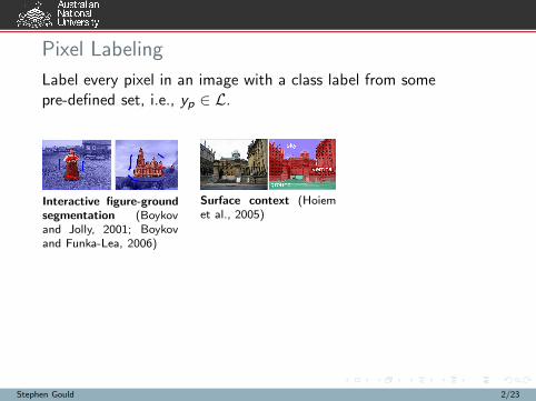
Label every pixel in an image with a class label from somepre-defined set, i.e., yp ∈ L.

Interactive figure-groundsegmentation (Boykovand Jolly, 2001; Boykovand Funka-Lea, 2006)

Surface context (Hoiemet al., 2005)

Semantic labeling (He etal., 2004; Shotton et al.,2006; Gould et al., 2009)

Stephen Gould 2/23

Pixel Labeling

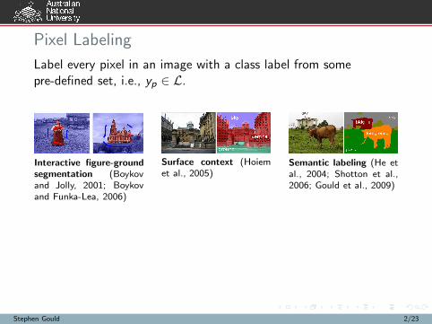
Label every pixel in an image with a class label from somepre-defined set, i.e., yp ∈ L.

Interactive figure-groundsegmentation (Boykovand Jolly, 2001; Boykovand Funka-Lea, 2006)

Surface context (Hoiemet al., 2005)

Semantic labeling (He etal., 2004; Shotton et al.,2006; Gould et al., 2009)

Stereo matching (Scharstein and Szeliski,2002)

Stephen Gould 2/23

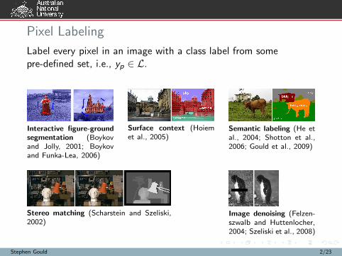
Pixel Labeling

Label every pixel in an image with a class label from somepre-defined set, i.e., yp ∈ L.

Interactive figure-groundsegmentation (Boykovand Jolly, 2001; Boykovand Funka-Lea, 2006)

Surface context (Hoiemet al., 2005)

Semantic labeling (He etal., 2004; Shotton et al.,2006; Gould et al., 2009)

Stereo matching (Scharstein and Szeliski,2002)

Image denoising (Felzen-szwalb and Huttenlocher,2004; Szeliski et al., 2008)

Stephen Gould 2/23

Digital Photo Montage

(Agarwala et al., 2004)

Stephen Gould 3/23

Digital Photo Montage

demonstration

Stephen Gould 4/23

Tutorial Overview

Part 1. Pairwise conditional Markov random fields for thepixel labeling problem (45 minutes)

Part 2. Pseudo-boolean functions and graph-cuts (1 hour)

Part 3. Higher-order terms and inference as integerprogramming (30 minutes)

please ask lots of questions

Stephen Gould 5/23

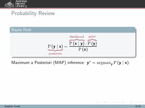
Probability Review

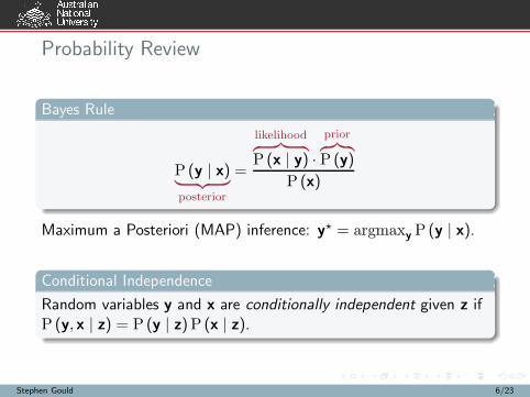
Bayes Rule

P (y | x)︸ ︷︷ ︸

posterior

=

likelihood︷ ︸︸ ︷

P (x | y) ·

prior︷ ︸︸ ︷

P (y)

P (x)

Maximum a Posteriori (MAP) inference: y⋆ = argmaxy P (y | x).

Stephen Gould 6/23

Probability Review

Bayes Rule

P (y | x)︸ ︷︷ ︸

posterior

=

likelihood︷ ︸︸ ︷

P (x | y) ·

prior︷ ︸︸ ︷

P (y)

P (x)

Maximum a Posteriori (MAP) inference: y⋆ = argmaxy P (y | x).

Conditional Independence

Random variables y and x are conditionally independent given z ifP (y, x | z) = P (y | z)P (x | z).

Stephen Gould 6/23

Graphical Models

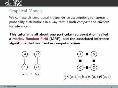
We can exploit conditional independence assumptions to representprobability distributions in a way that is both compact and efficient

for inference.

This tutorial is all about one particular representation, calleda Markov Random Field (MRF), and the associated inferencealgorithms that are used in computer vision.

A B

C D

a ⊥⊥ d | b, c

A � B

� �

C � D

1

ZΨ(a, b)Ψ(b, d)Ψ(d , c)Ψ(c , a)

Stephen Gould 7/23

Graphical Models

A � B

� �

C � D

P (a, b, c , d) =1

ZΨ(a, b)Ψ(b, d)Ψ(d , c)Ψ(c , a)

=1

Zexp {−ψ(a, b)− ψ(b, d) − ψ(d , c) − ψ(c , a)}

where ψ = − log Ψ.

Stephen Gould 8/23

Energy Functions

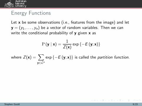
Let x be some observations (i.e., features from the image) and lety = (y1, . . . , yn) be a vector of random variables. Then we canwrite the conditional probability of y given x as

P (y | x) =1

Z (x)exp {−E (y; x)}

where Z (x) =∑

y∈Ln

exp {−E (y; x)} is called the partition function.

Stephen Gould 9/23

Energy Functions

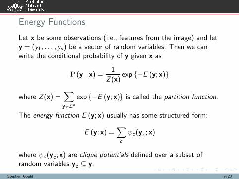
Let x be some observations (i.e., features from the image) and lety = (y1, . . . , yn) be a vector of random variables. Then we canwrite the conditional probability of y given x as

P (y | x) =1

Z (x)exp {−E (y; x)}

where Z (x) =∑

y∈Ln

exp {−E (y; x)} is called the partition function.

The energy function E (y; x) usually has some structured form:

E (y; x) =∑

c

ψc(yc ; x)

where ψc (yc ; x) are clique potentials defined over a subset ofrandom variables yc ⊆ y.

Stephen Gould 9/23

Conditional Markov Random Fields

E (y; x) =∑

c

ψc(yc ; x)

=∑

i∈V

ψUi (yi ; x)

︸ ︷︷ ︸

unary

+∑

ij∈E

ψPij (yi , yj ; x)

︸ ︷︷ ︸

pairwise

+∑

c∈C

ψHc (yc ; x).

︸ ︷︷ ︸

higher-order

x1 x2 x3

y1 y2 y3

x4 x5 x6

y4 y5 y6

x7 x8 x9

y7 y8 y9

Stephen Gould 10/23

Pixel Neighbourhoods

y1 y2 y3

y4 y5 y6

y7 y8 y9

4-connected, N4

y1 y2 y3

y4 y5 y6

y7 y8 y9

8-connected, N8

Stephen Gould 11/23

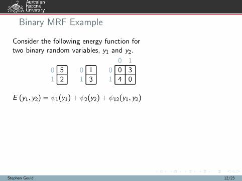
Binary MRF Example

Consider the following energy function fortwo binary random variables, y1 and y2.

01

5

2

01

1

3

01

0 1

0 3

4 0

E (y1, y2) = ψ1(y1) + ψ2(y2) + ψ12(y1, y2)

Stephen Gould 12/23

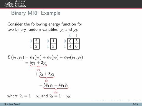
Binary MRF Example

Consider the following energy function fortwo binary random variables, y1 and y2.

01

5

2

01

1

3

01

0 1

0 3

4 0

E (y1, y2) = ψ1(y1) + ψ2(y2) + ψ12(y1, y2)= 5y1 + 2y1

︸ ︷︷ ︸

ψ1

+ y2 + 3y2︸ ︷︷ ︸

ψ2

+ 3y1y2 + 4y1y2︸ ︷︷ ︸

ψ12

where y1 = 1− y1 and y2 = 1− y2.

Stephen Gould 12/23

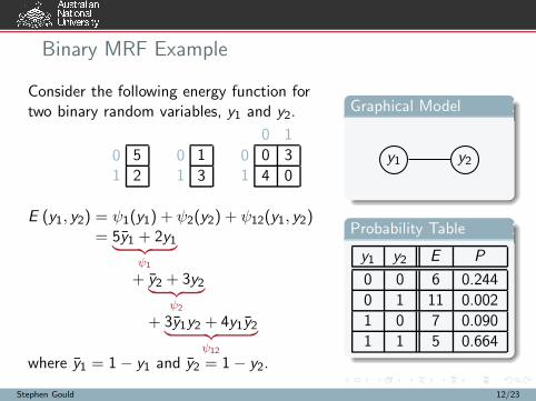
Binary MRF Example

Consider the following energy function fortwo binary random variables, y1 and y2.

01

5

2

01

1

3

01

0 1

0 3

4 0

E (y1, y2) = ψ1(y1) + ψ2(y2) + ψ12(y1, y2)= 5y1 + 2y1

︸ ︷︷ ︸

ψ1

+ y2 + 3y2︸ ︷︷ ︸

ψ2

+ 3y1y2 + 4y1y2︸ ︷︷ ︸

ψ12

where y1 = 1− y1 and y2 = 1− y2.

Graphical Model

y1 y2

Probability Table

y1 y2 E P

0 0 6 0.244

0 1 11 0.002

1 0 7 0.090

1 1 5 0.664

Stephen Gould 12/23

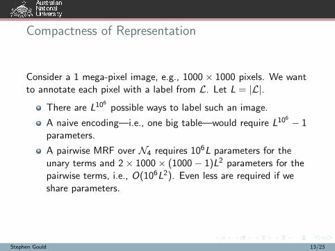
Compactness of Representation

Consider a 1 mega-pixel image, e.g., 1000 × 1000 pixels. We wantto annotate each pixel with a label from L. Let L = |L|.

There are L106possible ways to label such an image.

A naive encoding—i.e., one big table—would require L106− 1

parameters.

A pairwise MRF over N4 requires 106L parameters for theunary terms and 2× 1000 × (1000 − 1)L2 parameters for thepairwise terms, i.e., O(106L2). Even less are required if weshare parameters.

Stephen Gould 13/23

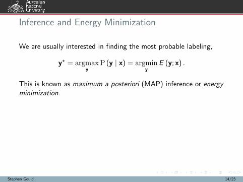
Inference and Energy Minimization

We are usually interested in finding the most probable labeling,

y⋆ = argmaxy

P (y | x) = argminy

E (y; x) .

This is known as maximum a posteriori (MAP) inference or energyminimization.

Stephen Gould 14/23

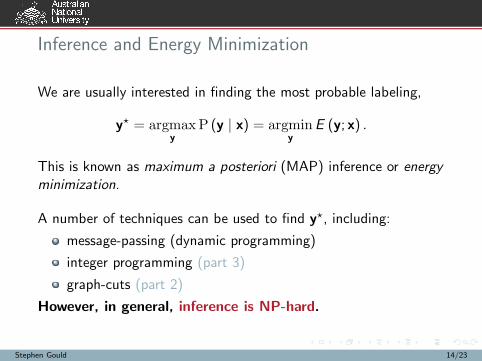
Inference and Energy Minimization

We are usually interested in finding the most probable labeling,

y⋆ = argmaxy

P (y | x) = argminy

E (y; x) .

This is known as maximum a posteriori (MAP) inference or energyminimization.

A number of techniques can be used to find y⋆, including:

message-passing (dynamic programming)

integer programming (part 3)

graph-cuts (part 2)

However, in general, inference is NP-hard.

Stephen Gould 14/23

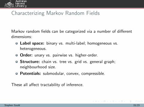
Characterizing Markov Random Fields

Markov random fields can be categorized via a number of differentdimensions:

Label space: binary vs. multi-label; homogeneous vs.heterogeneous.

Order: unary vs. pairwise vs. higher-order.

Structure: chain vs. tree vs. grid vs. general graph;neighbourhood size.

Potentials: submodular, convex, compressible.

These all affect tractability of inference.

Stephen Gould 15/23

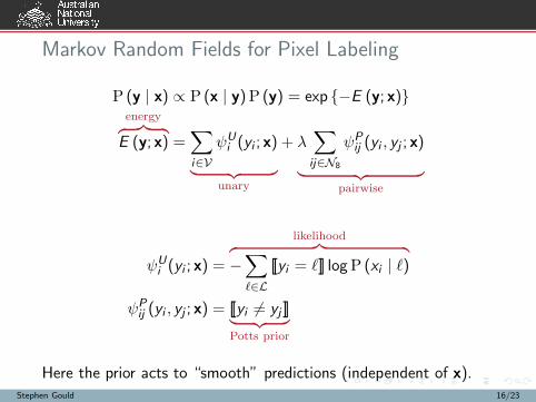
Markov Random Fields for Pixel Labeling

P (y | x) ∝ P (x | y)P (y) = exp {−E (y; x)}energy︷ ︸︸ ︷

E (y; x) =∑

i∈V

ψUi (yi ; x)

︸ ︷︷ ︸

unary

+ λ∑

ij∈N8

ψPij (yi , yj ; x)

︸ ︷︷ ︸

pairwise

ψUi (yi ; x) =

likelihood︷ ︸︸ ︷

−∑

ℓ∈L

[[yi = ℓ]] logP (xi | ℓ)

ψPij (yi , yj ; x) = [[yi 6= yj ]]

︸ ︷︷ ︸

Potts prior

Here the prior acts to “smooth” predictions (independent of x).

Stephen Gould 16/23

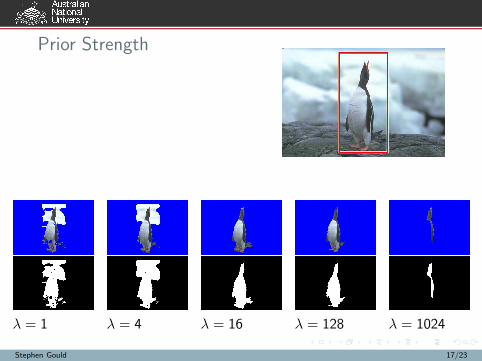
Prior Strength

λ = 1 λ = 4 λ = 16 λ = 128 λ = 1024

Stephen Gould 17/23

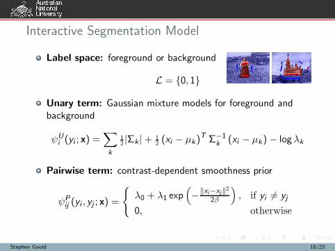
Interactive Segmentation Model

Label space: foreground or background

L = {0, 1}

Unary term: Gaussian mixture models for foreground andbackground

ψUi (yi ; x) =

∑

k

12|Σk |+ 1

2(xi − µk)

T Σ−1k

(xi − µk)− log λk

Pairwise term: contrast-dependent smoothness prior

ψPij (yi , yj ; x) =

{

λ0 + λ1 exp(

−‖xi−xj‖

2

2β

)

, if yi 6= yj

0, otherwise

Stephen Gould 18/23

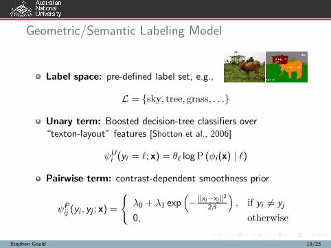
Geometric/Semantic Labeling Model

Label space: pre-defined label set, e.g.,

L = {sky, tree, grass, . . .}

Unary term: Boosted decision-tree classifiers over“texton-layout” features [Shotton et al., 2006]

ψUi (yi = ℓ; x) = θℓ logP (φi(x) | ℓ)

Pairwise term: contrast-dependent smoothness prior

ψPij (yi , yj ; x) =

{

λ0 + λ1 exp(

−‖xi−xj‖2

2β

)

, if yi 6= yj

0, otherwise

Stephen Gould 19/23

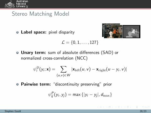
Stereo Matching Model

Label space: pixel disparity

L = {0, 1, . . . , 127}

Unary term: sum of absolute differences (SAD) ornormalized cross-correlation (NCC)

ψUi (yi ; x) =

∑

(u,v)∈W

|xleft(u, v)− xright(u − yi , v)|

Pairwise term: “discontinuity preserving” prior

ψPij (yi , yj ) = max {|yi − yj |, dmax}

Stephen Gould 20/23

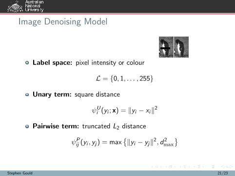
Image Denoising Model

Label space: pixel intensity or colour

L = {0, 1, . . . , 255}

Unary term: square distance

ψUi (yi ; x) = ‖yi − xi‖

2

Pairwise term: truncated L2 distance

ψPij (yi , yj) = max

{‖yi − yj‖

2, d2max

}

Stephen Gould 21/23

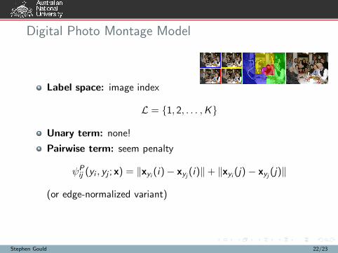
Digital Photo Montage Model

Label space: image index

L = {1, 2, . . . ,K}

Unary term: none!

Pairwise term: seem penalty

ψPij (yi , yj ; x) = ‖xyi (i)− xyj (i)‖+ ‖xyi (j) − xyj (j)‖

(or edge-normalized variant)

Stephen Gould 22/23

end of part 1

Stephen Gould 23/23