markov - uni-bonn.dewt.iam.uni-bonn.de/.../people/Anton_Bovier/lecture-notes/markov.pdf · 4.2 Strong and weak solutions ... 6.7 The one-dimensional trap model and a singular

Anton Bovier

Markov Processes

Lecture Notes Summer 2012, Bonn

November 24, 2012

Contents

1 Markov processes in discrete time. . . . . . . . . . . . . . . . . . . . . . . . . . . . . . . . 11.1 Markov processes with stationary transition probabilities . . . . . . . . . 21.2 The strong Markov property . . . . . . . . . . . . . . . . . . . . . . . . .. . . . . . . . 41.3 Markov processes and martingales . . . . . . . . . . . . . . . . . . .. . . . . . . . . 41.4 Harmonic functions and martingales . . . . . . . . . . . . . . . . .. . . . . . . . . . 81.5 Dirichlet problems . . . . . . . . . . . . . . . . . . . . . . . . . . . . . . .. . . . . . . . . . . 91.6 Feynman-Kac formulas . . . . . . . . . . . . . . . . . . . . . . . . . . . . .. . . . . . . . 121.7 Doob’sh-transform . . . . . . . . . . . . . . . . . . . . . . . . . . . . . . . . . . . . . . . . .13

2 Continuous time martingales. . . . . . . . . . . . . . . . . . . . . . . . . . . . . . . . . . . . 172.1 Càdlàg functions . . . . . . . . . . . . . . . . . . . . . . . . . . . . . . . . .. . . . . . . . . . 172.2 Filtrations, supermartingales, and càdlàg processes .. . . . . . . . . . . . . 192.3 Doob’s regularity theorem . . . . . . . . . . . . . . . . . . . . . . . . .. . . . . . . . . . 202.4 Stopping times . . . . . . . . . . . . . . . . . . . . . . . . . . . . . . . . . . .. . . . . . . . . . 242.5 Entrance and hitting times . . . . . . . . . . . . . . . . . . . . . . . . .. . . . . . . . . . 262.6 Optional stopping and optional sampling . . . . . . . . . . . . .. . . . . . . . . . 27

3 Markov processes in continuous time. . . . . . . . . . . . . . . . . . . . . . . . . . . . . 313.1 Markov jump processes . . . . . . . . . . . . . . . . . . . . . . . . . . . . .. . . . . . . . 323.2 Semi-groups, resolvents, generators . . . . . . . . . . . . . . .. . . . . . . . . . . . 35

3.2.1 Transition functions and semi-groups . . . . . . . . . . . . .. . . . . . 353.2.2 Strongly continuous contraction semi-groups . . . . . .. . . . . . . 383.2.3 The Hille-Yosida theorem . . . . . . . . . . . . . . . . . . . . . . . .. . . . . 40

3.3 Feller-Dynkin processes . . . . . . . . . . . . . . . . . . . . . . . . . .. . . . . . . . . . . 493.4 The strong Markov property . . . . . . . . . . . . . . . . . . . . . . . . .. . . . . . . . 533.5 The martingale problem . . . . . . . . . . . . . . . . . . . . . . . . . . . .. . . . . . . . . 54

3.5.1 Uniqueness . . . . . . . . . . . . . . . . . . . . . . . . . . . . . . . . . . . .. . . . . 603.5.2 Existence . . . . . . . . . . . . . . . . . . . . . . . . . . . . . . . . . . . . .. . . . . . 69

v

vi Contents

4 Stochastic differential equations. . . . . . . . . . . . . . . . . . . . . . . . . . . . . . . . . 734.1 Stochastic integral equations . . . . . . . . . . . . . . . . . . . . .. . . . . . . . . . . . 734.2 Strong and weak solutions . . . . . . . . . . . . . . . . . . . . . . . . . .. . . . . . . . . 734.3 Weak solutions and the martingale problem . . . . . . . . . . . .. . . . . . . . . 794.4 Weak solutions from Girsanov’s theorem . . . . . . . . . . . . . .. . . . . . . . . 874.5 Large deviations . . . . . . . . . . . . . . . . . . . . . . . . . . . . . . . . .. . . . . . . . . . 894.6 SDE’s from conditioning: Doob’sh-transform . . . . . . . . . . . . . . . . . . 95

5 SDE’s and partial differential equations . . . . . . . . . . . . . . . . . . . . . . . . . . 995.1 The Dirichlet problem. . . . . . . . . . . . . . . . . . . . . . . . . . . . .. . . . . . . . . . 995.2 Maximum principle and Harnack-inequalities . . . . . . . . .. . . . . . . . . . 108

6 Reversible diffusions . . . . . . . . . . . . . . . . . . . . . . . . . . . . . . . . . . . . . . . . . . . 1116.1 Reversibility . . . . . . . . . . . . . . . . . . . . . . . . . . . . . . . . . . .. . . . . . . . . . . . 1116.2 Reversible diffusions . . . . . . . . . . . . . . . . . . . . . . . . . . . .. . . . . . . . . . . . 1136.3 Equilibrium measure, equilibrium potential, and capacity . . . . . . . . . 1156.4 The case of dimension one. . . . . . . . . . . . . . . . . . . . . . . . . . .. . . . . . . . 1216.5 Another view on one-dimensional diffusions . . . . . . . . . .. . . . . . . . . . 1246.6 Brownian local time and speed measures . . . . . . . . . . . . . . .. . . . . . . . 1266.7 The one-dimensional trap model and a singular diffusion. . . . . . . . . 128

7 Appendix: Weak convergence. . . . . . . . . . . . . . . . . . . . . . . . . . . . . . . . . . . . 1357.1 Some topology . . . . . . . . . . . . . . . . . . . . . . . . . . . . . . . . . . . .. . . . . . . . . 1357.2 Polish and Lousin spaces . . . . . . . . . . . . . . . . . . . . . . . . . . .. . . . . . . . . 1377.3 The càdlàg spaceDE[0,∞) . . . . . . . . . . . . . . . . . . . . . . . . . . . . . . . . . . . 147

7.3.1 A Skorokhod metric . . . . . . . . . . . . . . . . . . . . . . . . . . . . . .. . . . 147

References. . . . . . . . . . . . . . . . . . . . . . . . . . . . . . . . . . . . . . . . . . . . . . . . . . .. . . . . . 151

Index . . . . . . . . . . . . . . . . . . . . . . . . . . . . . . . . . . . . . . . . . . . . . . . . . . .. . . . . . . . . . 153

Chapter 1Markov processes in discrete time

Markov processes are among the most important stochastic processes that are usedto model real live phenomena that involve disorder. This is because the constructionof these processes is very much adapted to our thinking aboutsuch processes. More-over, Markov processes can be very easily implemented in numerical algorithms.This allows to numerically simulate even very complicated systems. We will alwaysimagine a Markov process as a “particle” moving around in state space; mind, how-ever, that these “particles” can represent all kinds of verycomplicated things, oncewe allow the state space to be sufficiently general.

Markov processes can be classified according to the properties of the nature oftime and the properties of their state space. Roughly, we have the following cate-gories:

(i) discrete time, finite state space(ii)discrete time, countable state space(iii)discrete time, general state space(iv)continuous time, countable state space(v)continuous time, general state space

The case (i) is elementary and can be studied with the help of elementary lin-ear algebra. Case (ii) is already much more interesting, andbrings new conceptssuch asrecurrenceandtransience. Case (iii) is really not all that more complicated,although there are new concepts with regard to all ergodicity problems. Case (iv)is not all that different from case (ii), and the construction basically start from adiscrete time Markov process where each unit of time is replaced by an exponen-tially distributed random time, whose parameter depends onthe position in space.Fundamentally new issues here can arise if these parametersare unbounded fromabove or not bounded away from zero. Case (v) is really new, and poses challeng-ing new problems that require some serious tools from functional analysis. A keynew problem here is how to describe such a process in simple terms. You alreadyknow some important examples from stochastic analysis: Brownian motion, Lévyprocesses, and processes that are built from these: strong solutions of stochastic

1

2 1 Markov processes in discrete time

differential equations. However, this is not all there is, and in this lecture we willdevelop a more general theory of continuous time Markov processes.

As a warm-up, we recall in this first chapter the theory of Markov processes withdiscrete time with a slightly different twist.

1.1 Markov processes with stationary transition probabilities

In the following we denote byS the state space which we assume to be a Polishspace.B denotes the Borel-σ -algebra onS.

The main building block for a Markov process is the so-calledtransition kernel.

Definition 1.1. A (one step) transition kernel for a discrete time Markov processwith state spaceS is a map,P : N0×S×B → [0,1], with the following properties:

(i) For eacht ∈ N0 andx∈ S, Pt(x, ·) is a probability measure on(S,B).(ii)For eachA∈ B, andt ∈ N0, Pt(·,A) is aB-measurable function onS.

Definition 1.2. A stochastic processX with state spaceSand index setN0 is a dis-crete time Markov process with transition kernelP if, for all A∈ B, t ∈ N,

P(Xt ∈ A|Ft−1)(ω) = Pt−1(Xt−1(ω),A),P−a.s.. (1.1.1)

HereFtt∈N0 denotes theσ -algebra generated by the random variablesX0, . . . ,Xt .

This requirement fixes the lawP up to one more probability measure on(S,B),the so-calledinitial distribution, P0.

Theorem 1.3.Let (S,B) be a Polish space and letP be a transition kernel andP0 a probability measure on(S,B). Then there exists a unique stochastic processsatisfying (1.1.1) andP(X0 ∈ A) = P0(A), for all A.

In general, we call a stochastic process whose index set supports the action of agroup (or semi-group)stationary(with respect to the action of this (semi) group, ifall finite dimensional distributions are invariant under the simultaneous shift of alltime-indices. Specifically, if our index sets,I , areR+ orZ, resp.N, then a stochasticprocess is stationary if for allℓ ∈ N, s1, . . . ,sℓ ∈ I , all A1 . . . ,Aℓ ∈ B, and allt ∈ I ,

P[Xs1 ∈ A1, . . . ,Xsℓ ∈ Aℓ

]= P

[Xs1+t ∈ A1, . . . ,Xsℓ+t ∈ Aℓ

]. (1.1.2)

We can express this also as follows: Define the shiftθ , for anyt ∈ I , as(X θt)s≡Xt+s. ThenX is stationary, if and only if, for allt ∈ I , the processesX andX θt

have the same finite dimensional distributions.In the case of Markov processes, a necessary (but not sufficient) condition for

stationarity is the stationarity of the transitions kernels.

1.1 Markov processes with stationary transition probabilities 3

Definition 1.4. A Markov process with discrete timeN0 and state spaceS is said tohavestationary transition probabilities (kernels), if its one step transition kernelPt

is independent oft, i.e., if there is a probability kernelP(x,A)

Pt(x,A) = P(x,A), (1.1.3)

for all t ∈ N, x∈ S, andA∈ B.

Remark 1.5.With the notationPt,s for the transitions kernel from times to timet,i.e.

P(Xt ∈ A|Fs) = Pt,s(A,Xs),

we could alternatively state that a Markov process hasstationary transition proba-bilities (kernels), if there exists a family of transition kernelsPt(x,A), s.t.

Ps,t(x,A) = Pt−s(x,A), (1.1.4)

for all s< t ∈N, x∈ S, andA∈ B. Note that there is a potential conflict of notationbetweenPt andPt which should not be confused.

A key concept for Markov processes with stationary transition kernels is the no-tion of aninvariantdistribution.

Definition 1.6. Let P be the transition kernel of a Markov process with stationarytransition kernels. Then a probability measure,π , on (S,B) is called an invariant(probability) distribution, if

∫π(dx)P(x,A) = π(A), (1.1.5)

for all A∈ B. More generally, a positive,σ -finite measure,π , satisfying (1.1.5), iscalled aninvariant measure.

Lemma 1.7.A Markov process with stationary probability kernels and initial dis-tribution P0 = π is a stationary stochastic process, if and only ifπ is an invariantprobability distribution.

Proof. Exercise. ⊓⊔

In the case when the state space,S, is finite, we have seen that there is always atleast one invariant measure, which then can be chosen to be a probability measure. Inthe case of general state spaces, while there still will always be an invariant measure(through a generalisation of the Perron-Frobenius theoremto the operator setting),there appears a new issue, namely whether there is an invariant measure that is finite,viz. whether there exists a invariant probability distribution.


1.2 The strong Markov property

The setting of Markov processes is very much suitable for theapplication of thenotions of stopping times. Recall that for a closed set,D, we set

τD ≡ inf (t > 0 : Xt ∈ D) . (1.2.1)

In fact, one of the very important properties of Markov processes is the fact that wecan split expectations between past and future also at stopping times.

Theorem 1.8.Let X be a Markov process with stationary transition kernels. LetFn

be a filtration such that X is adapted, and let T be a stopping time. Let F and G beF -measurable functions, and let F in addition be measurable with respect to thepre-T-σ -algebraFT . Then

E [1IT<∞FGθT |F0] = E[1IT<∞FE′ [G|F ′

0

](XT)

∣∣F0]

(1.2.2)

whereE′ andF ′ refer to an independent copy, X′, of the Markov process X.

Proof. We have

E [1IT<∞FGθT |F0] (1.2.3)

= E [E [1IT<∞FGθT |FT ] |F0]

= E [1IT<∞FE [GθT |FT ] |F0] .

Now E [GθT |FT ] depends only onXT (and will thus often be denoted simply asE [GθT|XT ]) and by stationarity is equal toE′ [G|F ′

0] (XT), which yields the claimof the theorem. ⊓⊔

1.3 Markov processes and martingales

We now take a different look at Markov processes that will become important andmore difficult in the continuous time case. First we want to see how the transitionkernels can be seen as operators acting on spaces of measuresrespectively spacesof function.

If µ is a σ -finite measure onS, andP is a Markov transition kernel, we definethe measureµP as

µP(A)≡∫

SP(x,A)µ(dx), (1.3.1)

and similarly, for thet-step transition kernel,Pt ,

µPt(A)≡∫

SPt(x,A)µ(dx). (1.3.2)

By the Markov property, we have

1.3 Markov processes and martingales 5

µPt(A) = µPt(A). (1.3.3)

Note that the action of ? on measures conserves the total mass, i.e.

µP(Σ) =

∫

SP(x,S)µ(dx) = µ(S). (1.3.4)

The action on measures has of course the following natural interpretation in termsof the process: ifP(X0 ∈ A) = µ(A), then

µ(Xt ∈ A) = µPt(A). (1.3.5)

Alternatively, if f is a bounded, measurable function onS, we define

(P f)(x)≡∫

Sf (y)P(x,dy), (1.3.6)

and(Pt f )(x) ≡

∫

Sf (y)Pt(x,dy), (1.3.7)

where againPt f = Pt f . (1.3.8)

Lemma 1.9.Let ‖ f‖∞ ≡ supx∈S| f (x) denote the supremums norm. Then for anybounded function f ,

‖P f‖∞ ≤ ‖ f‖∞. (1.3.9)

Proof. Simply note that

‖P f‖∞ =

∥∥∥∥∫

SP(x,dy) f (y)

∥∥∥∥∞≤ ‖ f‖∞

∫

SP(x,dy) = ‖ f‖∞. (1.3.10)

⊓⊔

We say thatPt is a semi-group acting on the space of measures, respectivelyon the space of bounded measurable functions. The interpretation of the action onfunctions is given as follows.

Lemma 1.10.Let Pt be a Markov semi-group acting on bounded measurable func-tions f . Then

(Pt f )(x) = E( f (Xt)|F0)(x)≡ Ex f (Xt ). (1.3.11)

Proof. We only need to show this fort = 1. Then, by definition,

Ex f (X1) =∫

Sf (y)P[X1 ∈ dy|F0](x) =

∫

Sf (y)P(x,dy).

⊓⊔

Notice that, by telescopic expansion, we have the elementary formula


Pt f − f =t−1

∑s=0

Ps(P−1I) f ≡t−1

∑s=0

PsL f , (1.3.12)

where we callL≡P−1I the (discrete) generator of our Markov process (this formulawill have a complete analog in the continuous-time case).

An interesting consequence is the following observation:

Lemma 1.11.[Discrete time martingale problem]. Let L be the generator of aMarkov process, Xt , and let f be a bounded measurable function. Then

Mt ≡ f (Xt)− f (X0)−t−1

∑s=0

L f (Xs) (1.3.13)

is a martingale.

Proof. Let t, r ≥ 0. Then

E(Mt+r |Ft ) = E( f (Xt+r )|Ft )−E( f (X0)|Ft )−t+r−1

∑s=0

E(L f (Xs)|Ft )

= Pr f (Xt )− f (Xt)+ f (Xt)− f (X0)

−t+r−1

∑s=t

E(L f (Xs)|Ft)−t−1

∑s=0

E(L f (Xs)|Ft )

= f (Xt )− f (X0)−t−1

∑s=0

(L f (Xs)

+Pr f (Xt)− f (Xt)−r−1

∑s=0

Ps(L f (Xt ))

= Mt +0. (1.3.14)

This proves the lemma.⊓⊔

Remark 1.12.(1.3.13) is of course the Doob decomposition of the processf (Xt ),since∑t−1

s=0L f (Xs) is a previsible process.

What is important about this observation is that it gives rise to a characterisationof the generator that will be extremely useful in the generalcontinuous time setting.

Namely, one can ask whether the requirement thatMt be a martingale given afamily of pairs( f ,L f ) characterises fully a Markov process.

Theorem 1.13.Let X be a discrete time stochastic process on a filtered spacesuchthat X is adapted. Then X is a Markov process with transition kernel P≡ 1I+L, ifand only if, for all bounded measurable functions, f , the expression on the right-hand side of (1.3.13) is a martingale.

1.3 Markov processes and martingales 7

Proof. Lemma 1.11 already provides the “only if” part, so it remainsto show the“if” part.

First, if we assume thatX is a Markov process, settingr = 1 in (1.3.13) andtaking conditional expectations givenF0, we see thatE f (X1)− f (X0) = (L f )(X0),implying that the transition kernel must be 1I+L.

It remains to show thatX is indeed a Markov process. To see this, we just use theabove calculation, which gives

E( f (Xt+r )|Ft ) = E(Mt+r |Ft)+ f (X0)

+t−1

∑s=0

(L f )(Xs)+t+r−1

∑s=t

E((L f )(Xs)|Ft)

= Mt + f (X0)+t−1

∑s=0

(L f )(Xs)+t+r−1

∑s=t

E((L f )(Xs)|Ft)

= f (Xt )+r−1

∑s=0

E((L f )(Xt+s)|Ft) (1.3.15)

Now let againr = 1. Then

E( f (Xt+1)|Ft) = f (Xt)+ (L f )(Xt) = ((1I+L) f )(Xt )≡ P f(Xt), (1.3.16)

In view of the definition of discrete time Markov processes, choosing f = 1IA, forA∈ B(S), this gives (1.1.1), and henceX is a Markov process. Thus the theorem isproven. ⊓⊔

In view of continuous time Markov processes it is, however, instructive to seethat we can also derive easily the more general fomula

E( f (Xt+s)|Ft) = (1I+L)s f (Xt )≡ Ps f (Xt ), (1.3.17)

from the martingale problem. We have seen that it holds fors= 1; Now proceed byinduction: assume that it holds for all bounded measurable functions fors≤ r −1.We must show that it then also holds fors= r. To do this, we use (1.3.15) and usethe induction hypothesis for the terms in the sum (wheres≤ r −1) with f replacedby L f . This gives

E( f (Xt+r )|Ft) = f (Xt)+r−1

∑s=0

((1I+L)sL f )(Xt ) (1.3.18)

= f (Xt)+r−1

∑s=0

(((1I+L)s(L+1I) f )(Xt )− ((1I+L)s f )(Xt))

= ((1I+L)r f ) (Xt),

as claimed. Hence (1.3.17) holds for alls, by induction.

Remark 1.14.The analog of this theorem in the continuous time case will bring outthe full strength of this approach. A crucial point is that itwill not be necessary


to consider all bounded functions, but just sufficiently rich classes. This allows toformulate martingale problems even then one cannot write down the generator in aexplicit form. The idea of characterising Markov processesby the associated mar-tingale problem goes back to Stroock and Varadhan, see [16].

1.4 Harmonic functions and martingales

We have seen that measures that satisfyµL = 0 are of special importance in thetheory of Markov processes. Also of central importance are functions that satisfyL f = 0. In this section we will assume that the transition kernelsof our Markovprocesses have bounded support, so that for someK < ∞, |Xt+1−Xt | ≤ K < ∞ forall t.

Definition 1.15.Let L be the generator of a Markov process. A measurable functionthat satisfies

L f (x) = 0,∀x∈ S, (1.4.1)

is called aharmonic function. A function is calledsubharmonic(resp. super-harmonic, if L f ≥ 0, resp.L f ≤ 0.

Theorem 1.16.Let Xt be a Markov process with generator L. Then, a non-negativefunction f is

(i) harmonic, if and only if f(Xt ) is a martingale;(ii)subharmonic, if and only if f(Xt) is a submartingale;(iii)super-harmonic, if and only if f(Xt) is a supermartingale;

Proof. Simply use Lemma 1.11.⊓⊔

Remark 1.17.Theorem 1.16 establishes a profound relationship between potentialtheory and martingales. It also explains, the strange choice of super and sub in mar-tingale theory.

A nice application of the preceding result is the maximum principle.

Theorem 1.18.Let X be a Markov process and let D be a bounded open domainsuch thatEτDc < ∞. Assume that f is a non-negative subharmonic function on D.Then

supx∈D

f (x)≤ supx∈Dc

f (x). (1.4.2)

Proof. Let us defineT ≡ τDc. Then, f (XT) is a submartingale, and thus

E( f (XT)|F0)(x)≥ f (x). (1.4.3)

SinceXT ∈ Dc, it must be true that

1.5 Dirichlet problems 9

supy∈Dc

f (y)≥ E( f (XT)|F0)(x)≥ f (x), (1.4.4)

for all x∈ D, hence the claim of the theorem. Of course we used again the Doob’soptional stopping theorem.⊓⊔

The theorem says that (sub) harmonic functions take on theirmaximum on theboundary, since of course the setDc in (1.4.2) can be replaced by a subset,∂D ⊂ Dc

such thatPx(XT ∈ ∂D) = 1. The above proof is an example of how intrinsicallyanalytic results can be proven with probabilistic means. The next section will furtherdevelop this theme.

1.5 Dirichlet problems

Let us now consider a connected bounded open subset ofS. We define the stoppingtimeT ≡ τDc.

If g is a measurable function onD, we consider the Dirichlet problem associatedto a generator,L, of a Markov process,X:

−(L f )(x) = g(x), x∈ D, (1.5.1)

f (x) = 0, x∈ Dc.

Theorem 1.19.Assume thatET < ∞. Then (1.5.1) has a unique solution given by

f (x) = E

(T−1

∑t=0

g(Xt)∣∣F0

)(x) (1.5.2)

Proof. Consider the martingaleMt from Lemma 1.11. We know from Doob’s op-tional stopping theorem (see e.g. [15]) thatMT is also a martingale. Moreover,

MT = f (XT)− f (X0)−T−1

∑t=0

(L f )(Xt ) = 0− f (X0)−T−1

∑t=0

(L f )(Xt ). (1.5.3)

But we wantf such that−L f = g onD. Thus, (1.5.3) seen as a problem forf , reads

MT =− f (X0)+T−1

∑t=0

g(Xt). (1.5.4)

Taking expectations conditioned onF0, yields

0=− f (X0)+E

(T−1

∑t=0

g(Xt)∣∣F0

), (1.5.5)

or


f (x) = Ex

(T−1

∑t=0

g(Xt)

)(1.5.6)

Here we relied of course on Doob’s optimal stopping theorem forEMT = 0.Thus any solution of the Dirichlet problem is given by (1.5.6). To verify exis-

tence, we just need to check that (1.5.6) solves−L f = g onD. To do this we use theMarkov property “backwards”, to see that

P f(x) = PEx

(T−1

∑t=0

g(Xt)

)= Ex

[T−1

∑t=1

g(Xt)

](1.5.7)

= Ex

[T−1

∑t=0

g(Xt)

]−g(x) = f (x)−g(x).

⊓⊔We see that the Markov process produces a solution of the Dirichlet problem. We

can express the solution in terms of an integral kernel, called the Green’s kernel,GD(x,dy), as

f (x) =∫

GD(x,dy)g(y)≡ Ex

(T−1

∑t=0

g(Xt)

), (1.5.8)

or, in more explicit terms,

GD(x,dy) =∞

∑t=0

PtD(x,dy), (1.5.9)

where

PtD(x,dy) =

∫

DP(x,dz1)

∫

DP(z1,dz2)

∫

D. . .

∫

DP(zt−1,dy). (1.5.10)

Note that∫

D P(x,dz)< 1.The preceding theorem has an obvious extension to more complicated boundary

value problems.Let D ⊂ Sbe as above and specify functionsg: D →R, u: Dc →R andk: D →

[−k,∞) with k< 1. Consider the following set of equations for an unknown functionf :

(−L f )(x)+ k(x) f (x) = g(x), ∀x∈ D, (1.5.11)

f (x) = u(x), ∀x∈ Dc.

The following theorem provides a stochastic representation of the solution of suchDirichlet problems.

Theorem 1.20.Let X be a discrete-time Markov process with generator L. Assumethat D is such that

Ex[τDc(1− k)τDc

]< ∞. (1.5.12)

1.5 Dirichlet problems 11

Then the Dirichlet problem(1.5.11)has a unique solution given by

f (x) = Ex

[τDc−1

∑s=0

s

∏u=0

11+ k(Xu)

g(Xs)+τDc−1

∏u=0

11+ k(Xu)

u(XτDc)

].

Proof. The most convenient way to prove Theorem 1.20 is again via themartin-gale problem characterisation of Markov processes. Indeed, we check that, for anybounded functionf ,

Mt ≡t−1

∏s=0

11+ k(Xs)

f (Xt )− f (X0)

+t−1

∑s=0

s

∏u=0

11+ k(Xu)

[k(Xs) f (Xs)− (L f )(Xs)] (1.5.13)

is a martingale. Moreover, Doob’s optional stopping theorem applies forMτDc undercondition (1.5.12). Thus as before, iff solves the Dirichlet problem (1.5.11), it musthold that

0 = ExMτcD= Ex

(τDc−1

∏s=0

11+ k(Xs)

u(XτDc)− f (x)

+τDc−1

∑s=0

s

∏u=0

11+ k(Xu)

g(Xs)

), (1.5.14)

which implies that (1.5.13) must hold. Finally one shows that this solves the Equa-tion (1.5.11) as in the proof of Theorem 1.19.⊓⊔

Note that the solution to the Dirichlet problem is unique, unless the homogeneousproblem

(−L f )(x)+ k(x) f (x) = 0, ∀x∈ D,f (x) = 0, ∀x∈ Dc,

(1.5.15)

admits a non-zero solution. The most interesting case for usis whenk ≡ λ is con-stant. In that case, if (1.5.15) admits a non-zero solution,thenλ is called aneigen-valueand the corresponding solution aneigenfunctionof the Dirichlet problem.

Theorem 1.20 is a two way game: it allows to produce solutionsof analytic prob-lems in terms of stochastic processes, and it allows to compute interesting proba-bilistic problems analytically. As an example, assume thatDc=A∪Bwith A∩B= /0.Seth= 1IA. Then, clearly, forx∈ D,

Exh(XT) = Px(XT ∈ A)≡ Px(τA < τB), (1.5.16)

and soPx(XT ∈A) can be represented as the solution of the boundary value problem


(L f )(x) = 0, x∈ D, (1.5.17)

f (x) = 1, x∈ A,

f (x) = 0, x∈ B.

This is a generalisation of theruin problem for the random walk.Exercise.Derive the formula forPx(τA < τB) directly from the Markov propertywithout using Lemma 1.11.

1.6 Feynman-Kac formulas

The formalism expained in the preceding section has a usefulextension to the solu-tion of time-dependent problems of the form

∂t f (x, t)−L f (x, t)+ k(x) f (x, t) = g(x), x∈ S, t ∈ [0,T], (1.6.1)

f (x,T) = ψ(x), x∈ S, (1.6.2)

where∂t f (x, t) ≡ f (x, t)− f (x, t −1) denotes the discrete deriative with respect totime.k,g,ψ are given functions, andT is a fixed time.

To obtain a stochstic representation of the solution of suchequations, we proceedby extending the telescopic expansions that yield martingales to functionsf thatdepend on bothXt andt. This alows to show that

Mt ≡t−1

∏s=0

11+ k(Xs)

f (Xt , t)− f (X0,0) (1.6.3)

+t−1

∑s=0

s

∏u=0

11+ k(Xu)

[k(Xs) f (Xs,s)− (L f )(Xs,s)+ ∂s f (Xs,s)] ,

where∂s f (X,s)≡ f (X,s)− f (X,s−1), is a martingale. Therefore, fort < T,

E(MT |Ft) = Mt . (1.6.4)

Now the left-hand side of (1.6.4) is equal to

1.7 Doob’sh-transform 13

t−1

∏s=0

11+ k(Xs)

E

(T−1

∏s=t

11+ k(Xs)

ψ(XT)|Ft

)− f (X0,0) (1.6.5)

+t−1

∑s=0

s

∏u=0

11+ k(Xu)

g(Xs)

+T−1

∑s=t

t−1

∏u=0

11+ k(Xu)

E

( s

∏u=t

11+ k(Xu)

g(Xs)∣∣∣Ft

)

= Mt −t−1

∏s=0

11+ k(Xs)

f (Xt , t)

+t−1

∏s=0

11+ k(Xs)

E

(T−1

∏s=t

11+ k(Xs)

ψ(XT)+T−1

∑s=t

s

∏u=t

11+ k(Xu)

g(Xs)∣∣∣Ft

).

Thus we arrive at the representation of the solution of (1.6.1)

f (x, t) = E

(T−1

∏s=t

11+ k(Xs)

ψ(XT)+T−1

∑s=t

s

∏u=t

11+ k(Xu)

g(Xs)∣∣∣Ft

)(x). (1.6.6)

This representation is called aFeynman-Kac formula. In the case wheng≡ 0 andk≡ 0, it simplifies to

f (x, t) = E(ψ(XT)|Ft )(x) = Exψ(XT−t). (1.6.7)

So far we have considered the case without boundary conditions. From the deriva-tion above, it is, however, also easy to see how to deal with problems of the form

∂t f (x, t)−L f (x, t)+ k(x) f (x, t) = g(x), x∈ D, t ∈ [0,T], (1.6.8)

f (x, t) = ψ(x), x∈ Dc, t ∈ [0,T], (1.6.9)

f (x,T) = ψ(x), x∈ S.

Namely, defining the optional timeT ≡ T ∧ τDc , and noticing thatMT is always amartingale, we obtain Thus we arrive at the representation of the solution of (1.6.1)

f (x, t) = E

(T−1

∏s=t

11+ k(Xs)

ψ(XT)+T−1

∑s=t

s

∏u=t

11+ k(Xu)

g(Xs)∣∣∣Ft

)(x). (1.6.10)

1.7 Doob’sh-transform

Let us consider a Markov process,X, with generatorP−1. We may want to considermodifications of the process. One important type modification is to condition it toreach some set in particular places (e.g. consider a random walk in a finite interval;we may be interested to consider this walk conditioned on thefact that it exits on a


specific side of the interval; this may correspond to consider a sequence of gamesconditioned on the player to win).

How and when can we do this, and what is the nature of the resulting process?In particular, is the resulting process again a Markov process, and if so, what is itsgenerator?

As an example, let us try to condition a Markov process to hit adomainB for thefirst time in a subsetA⊂ B. We may assume thatEτB < ∞. Defineh(x) ≡ Px[τA =τB], if x 6∈ B. Let P be the law ofX. Let us define a new measure,Ph, on the spaceof paths as follows: IfY is aFt -measurable random variable, then

Eh[Y|F0] =1

h(X0)E[h(Xt)Y|F0]. (1.7.1)

Lemma 1.21.With the notation above, if Y is aFτB−1-measurable function,

Ehx[Y] = Ex[Y|τA = τB]. (1.7.2)

Proof. This is an application of the strong Markov property. By definition,

Ehx[Y] =

1h(x)

Ex[Yh(XτB−1)] (1.7.3)

=1

h(x)Ex[YE′[1IτA=τB|F ′

0](XτB−1)]

=1

h(x)Ex [YE [1IτA=τB|FτB−1]]

=1

Px[τA = τB]Ex [Y1IτA=τB]

= Ex[Y|τA = τB].

Here the first equality is just the definition ofh and reproduces the form of the right-hand side of the strong Markov property; the second equalityis the strong Markovproperty; the last equality uses that fact that the eventτA = τB depends only onwhat happens afterτB−1, and so 1IτA=τBθτB−1 = 1IτA=τB. ⊓⊔

Let us now look at the transformed measurePh in the general case. The first thingto check is of course whether this defines in a consistent way aprobability measure.Some thought shows that all that we need is the following lemma.

Lemma 1.22.Let Y beFs-measurable. Then, for any t≥ s,

Eh[Y|F0]≡1

h(X0)E[h(Xs)Y|F0] =

1h(X0)

E[h(Xt)Y|F0]. (1.7.4)

In particular,Ph[Ω |F0] = 1.

Proof. Just introduce a conditional expectation:

1.7 Doob’sh-transform 15

E[h(Xt)Y|F0] = E[E[h(Xt)Y|Fs]|F0] = E[YE[h(Xt)|Fs]|F0], (1.7.5)

and use thath(Xt) is a martingale

= E[Yh(Xs)|F0],

from which the result follows. ⊓⊔

This lemma shows in particular, why it is important thathbe a harmonic function.Now we turn to the question of whether the lawPh is a Markov process. To this

end we turn to the martingale problem. We will show that thereexists a generator,Lh, such that

Mht ≡ f (Xt )− f (X0)−

t−1

∑s=0

(Lh f )(Xs) (1.7.6)

is a martingale under the lawEh, i.e. that, fort > t ′,

Eh[Mht |Ft′ ] = Mh

t′ . (1.7.7)

Note first that, by definition

Eh[Mht |Ft′ ] =

1h(Xt′)

E[h(Xt) f (Xt)|Ft′ ]− f (X0)−t′−1

∑s=0

(Lh f )(Xs)

−t−1

∑s=t′

1h(Xt′)

E[h(Xs)Lh f (Xs)|Ft′ ]. (1.7.8)

The middle terms are part ofMht′ and we must considerE[ f (Xt)h(Xt)|Ft′ ]. This is

done by applying the martingale problem forP and the functionf h. This yields

E[ f (Xt)h(Xt)|Ft′ ] = f (Xt′ )h(Xt′)+t−1

∑s=t′

E[(L( f h))(Xs)|Ft′ ]

Inserting this in (1.7.8) gives

Eh[Mht |Ft′ ] = f (Xt′)− f (X0)−

t′−1

∑s=0

(Lh f )(Xs)

+1

h(Xt′)

t−1

∑s=t′

[E[(L( f h))(Xs)|Ft′ ]−E[h(Xs)L

h f (Xs)|Ft′ ]]

= Mht′

+1

h(Xt′)

t−1

∑s=t′

[E[(L( f h))(Xs)|Ft′ ]−E[h(Xs)L

h f (Xs)|Ft′ ]].

The second term will vanish if we chooseLh defined throughL f (x)= h(x)−1(L(h f))(x),i.e.


Lh f (x) ≡ 1h(x)

∫P(x,dy)h(y) f (y)− f (x). (1.7.9)

Hence we see that underPh, X solves the martingale problem corresponding tothe generatorLh, and so is a Markov process with transition kernelPh = Lh+1. TheprocessX underPh is called the (Doob)h-transform of the original Markov process.Exercise.As a simple example, consider a simple random walk on−N,−N+1, . . . ,N. Assume we want to condition this process on hitting+N before−N.Then let

h(x) = Px[τN = τN∪−N] = Px[τN < τ−N].

Computeh(x) and use this to compute the transition rates of theh-transformed walk?Plot the probabilities to jump down in the new process!

Chapter 2Continuous time martingales

Martingales play a truly fundamental rôle in the theory of stochastic processes indiscrete time, and in particular we have seen an intimate connection between mar-tingales and Markov processes. In this course we will seriously engage in the studyof continuous time processes where this relation will play an even more central rôle.Therefore, we begin with the extension of martingale theoryto the continuous timesetting. We will see that this will go quite smoothly, but we will have to worry abouta number of technical details. Most of the material in this Chapter is from Rogersand Williams [15].

2.1 Càdlàg functions

In the example of Brownian motion we have seen that we could construct this con-tinuous time process on the space of continuous functions. This setting is, however,too restrictive for the general theory. It is quite important to allow for stochasticprocesses to have jumps, and thus live on spaces of discontinuous paths. Our firstobjective is to introduce a sufficiently rich space of such functions that will still bemanageable.

Definition 2.1. A function f : R+ →R is called acàdlàg 1 function, iff

(i) for everyt ≥ 0, f (t) = lims↓t f (s), and(ii)for every t > 0, f (t−) = lims↑t f (s) exists.

Recall that this definition should remind you of distribution functions. In fact, aprobability distribution function is a non-decreasing càdlàg function.

It will be important to be able to extend functions specified on countable sets tocàdlàg functions.

Definition 2.2. A functiony : Q+ →R is calledregularisable, iff

1 From “continue à droite, limites à gauche”.

17

18 2 Continuous time martingales

(i) for everyt ≥ 0, limq↓t y(q) exists finitely, and(ii)for every t > 0, y(t−) = limq↑t y(s) exists finitely.

Regularisability is linked to properties of upcrossings. We define this importantconcept for functions from the rationals toR.

Definition 2.3. Let y : Q+ → R, N ∈ N and let a < b ∈ R. Then the numberUN(y, [a,b]) ∈ N∪ ∞ of upcrossings of[a,b] by y during the interval[0,N] isthe supremum over allk ∈ N, such that there are rational numbersqi, r i ∈ Q, i ≤ kwith the property that

0≤ q1 < r1 < · · ·< qk < rk ≤ N

andy(qi)< a< b< y(r i), for all 1≤ i ≤ k.

Theorem 2.4.Let y: Q+ → R. Then y is regularisable if and only if, for all N∈ N

and a< b∈ R,sup|y(q)| : q∈Q∩ [0,N]< ∞, (2.1.1)

andUN(y, [a,b])< ∞. (2.1.2)

Proof. Let us first show that the two conditions are sufficient. To do so, assumethat limsupq↓t y(q) > lim infq↓t y(q). Then chooseb> a such that limsupq↓t y(q) >b> a> lim infq↓y(q). Then, forN > t, y(q) must cross[a,b] infinitely many times,i.e.UN(y, [a,b]) = +∞, contradicting assumption (2.1.2). Thus the limit limq↓t y(q)exists, and by (2.1.1) it is finite. The same argument appliesto the limit from below.

Next we show that the conditions are necessary. Assume that for someN y(q) isunbounded on[0,N]. Then for anyn there existsqn such that|y(qn)| > n. The set∪nqn must be infinite, since otherwiseq will be infinite on a finite set, contradict-ing the assumption that it takes values inR. Hence this set has at least one accumu-lation point,t. But then either limq↑t y(q) or limq↓t y(q) must be infinite, hencey isnot regularisable.

Assume now thatUN(y; [a,b]) = ∞. Definet ≡ infr ∈ R+ : Ur(y; [a,b]) = ∞.Then there are infinitely many upcrossings of[a,b] in any interval[t − ε, t] or in theinterval[t, t + ε], for anyε > 0. In the first case, this implies that limsupq↑t y(y)≥ band liminfq↑t y(y) ≤ a, which precludes the existence of that limit. In the secondcase, the same argument precludes the existence of the limitlimq↓t y(y).

One of the main points of Theorem 2.4 is that it can be used to show that theproperty to be regularisable is measurable.

Corollary 2.5. Let Yq,q∈ Q+ be a stochastic process defined on(Ω ,F ,P) andlet

G≡ ω ∈ Ω : q→Yq(ω) is regularisable (2.1.3)

Then G∈ F .

2.2 Filtrations, supermartingales, and càdlàg processes 19

Proof. By Theorem 2.4, to check regularisability we have to take countable inter-sections and unions of finite dimensional cylinder sets which are all measurable.Thus regularisability is a measurable property.

Next we observe that from a regularisable function we can readily obtain a càdlàgfunction by taking limits from the right.

Theorem 2.6.Let y: Q+ → R be a regularisable function. Define, for any t∈ R+,

f (t)≡ limq↓t

y(q). (2.1.4)

Then f is càdlàg .

The proof is obvious and left to the reader.

2.2 Filtrations, supermartingales, and càdlàg processes

We begin with a probability space(Ω ,G ,P). We define a continuous time filtrationGt , t ∈ R+ essentially as in the discrete time case.

Definition 2.7. A filtration (Gt , t ∈R+) of (Ω ,G ,P) is an increasing family of sub-σ -algebrasGt , such that, for 0≤ s< t,

Gs ⊂ Gt ⊂ G∞ ≡ σ

(⋃

r∈R+

Gr

)⊂ G . (2.2.1)

We call(Ω ,G ,P;(Gt , t ∈ R+)) a filtered space.

Definition 2.8. A stochastic process,Xt , t ∈R+, is calledadaptedto the filtrationGt , t ∈ R+, if, for everyt, Xt is Gt -measurable.

Definition 2.9. A stochastic process,X, on a filtered space is called amartingale, ifand only if the following hold:

(i) The processX is adapted to the filtrationGt , t ∈ R+;(ii)For all t ∈ R+, E|Xt |< ∞;(iii)For all s≤ t ∈ R+,

E(Xt |Gs) = Xs, a.s.. (2.2.2)

Sub- and super-martingales are define in the same way, with “=” in (2.2.2) replacedby “≥” resp. “≤”.

We see that so far almost nothing changed with respect to the discrete time setup.Note in particular that if we take a monotone sequence of points tn, thenYn ≡ Xtn isa discrete time martingale (sub, super) wheneverXt is a continuous time martingale(sub, super).

The next lemma is important to connect martingale properties to càdlàg properties.


Lemma 2.10.Let Y be a supermartingale on a filtered space(Ω ,G ,P;(Gt , t ∈R+)).Let t∈ R+ and let q(−n), n∈ N, such that q(−n) ↓ t, as n↑ ∞. Then

limq(−n)↓t

Yq(−n)

exists a.s. and inL 1.

Proof. This is an application of the Lévy-Doob downward theorem (see [1], Thm.4.2.9).

Spaces of càdlàg functions are the natural setting for stochastic processes. Wedefine this in a strict way.

Definition 2.11.A stochastic process is called a càdlàg process, if all its samplepaths are càdlàg functions. càdlàg processes that are (super,sub) martingales arecalled càdlàg (super,sub) martingales.

Remark 2.12.Note that we do not just ask that almost all sample paths are càdlàg .

2.3 Doob’s regularity theorem

We will now show that the setting of càdlàg functions is in fact suitable for thetheory of martingales.

Theorem 2.13.Let (Yt , t ∈ R+) be a supermartingale defined on a filtered space(Ω ,G ,P,(Gt , t ∈R+)). Define the set

G≡ ω ∈ Ω : the mapQ+ ∋ q→Yq(ω) ∈ R is regularisable. (2.3.1)

Then G∈ G andP(G) = 1. The process X defined by

Xt(ω)≡

limq↓t Yq(ω), if ω ∈ G,

0, else(2.3.2)

is a càdlàg process.

Proof. The proof makes use of our observations in Theorem 2.4. Thereare onlycountably many triples(N,a,b) with N ∈ N, a< b∈ Q. Thus in view of Theorem2.4, we must show that with probability one,

supq∈Q∩[0,N]

|Yq|< ∞, (2.3.3)

andUN([a,b];Y|Q)< ∞, (2.3.4)

2.3 Doob’s regularity theorem 21

whereY|Q denotes the restriction ofY to the rational numbers.To do this, we will use discrete time approximations ofY. Let D(m)⊂Q∩ [0,N]

be an increasing sequence of finite subsets ofQ converging toQ∩ [0,N] asm↑ ∞.Then

P

[sup

q∈Q∩[0,N]

|Yq|> 3c

]= lim

m↑∞P

[sup

q∈D(m)

|Yq|> 3c

](2.3.5)

≤ c−1(4E|Y0|+3E|YN|) ,

by Lemma 4.4.15 in [1]. Takingc ↑ ∞ (2.3.3) follows. Note that we used the unifor-mity of the maximum inequality in the number of steps!

Similarly, using the upcrossing estimate of Theorem 4.2.2 in [1], we get that

E [UN([a,b];Y|Q] = limm↑∞

E[UN([a,b];Y|D(m))

]< ∞ ≤ E|YN|+ |a|

b−a, (2.3.6)

uniformly in m, and so (2.3.4) also follows.Now Theorem 2.4 implies the asserted result.

We may think that Theorem 2.13 solves all problems related tocontinuous timemartingales. Simply start with any supermartingale and then pass to the càdlàgregularization. However, a problem of measurability arises. This can be seen in themost trivial example of a process with a single jump. LetYt be defined for anyω ∈Ωas

Yt(ω) =

0, if t ≤ 1,

q(ω), if t > 1,(2.3.7)

whereEq = 0. Let Gt be the natural filtration associated to this process. Clearly,for t ≤ 1, Gt = /0,Ω. Yt is a martingale with respect to this filtration. The càdlàgversion of this process is

Xt(ω) =

0, if t < 1,

q(ω), if t ≥ 1,(2.3.8)

Now first, Xt is not adapted to the filtrationGt , sinceX1 is not measurable withrespect toG1. This problem can also not be remedied by a simple modification onsets of measure zero, sinceP[X1 =Y1]< 1. In particular,Xt is not a martingale withrespect to the filtrationGt , since

E[X1+ε |G1] = 0 6= X1.

We see that the right-continuous regularization ofY at the point of the jump an-ticipates information from the future. If we want to developour theory on càdlàgprocesses, we must take this into account and introduce a richer filtration that con-tains this information.


Definition 2.14.Let (Ω ,G ,P,(Gt , t ∈ R+)) be a filtered space. Define, for anyt ∈R+,

Gt+ ≡⋂

s>t

Gs =⋂

Q∋q>t

Gq (2.3.9)

and letN (G∞)≡ G∈ G∞ : P[G] ∈ 0,1 . (2.3.10)

Then thepartial augmentation, (Ht , t ∈ R+), of the filtrationGt is defined as

Ht ≡ σ(Gt+,N (G∞)). (2.3.11)

The following lemma, which is obvious from the constructionof càdlàg versions,justifies this definition.

Lemma 2.15.If Yt is a supermartingale with respect to the filtrationGt , and Xt

is its càdlàg version defined in Theorem 2.13, then Xt is adapted to the partiallyaugmented filtrationHt .

The natural question is whether in this settingXt is a supermartingale. The nexttheorem answers this question and is to be seen as the completion of Theorem 2.13

Theorem 2.16.With the assumptions and notations of Lemma 2.15, the process Xt

is a supermartingale with respect to the filtrationsHt . Moreover, X is a modificationof Y if and only if Y is right-continuous in the sense that, forevery t∈ R+,

lims↓t

E|Yt −Ys|= 0. (2.3.12)

Proof. This is now pretty straight-forward. Fixs > t, and take a decreasing se-quence,s> q(n) ∈Q, of rational points converging tot. Then

E[Ys|Gq(n)]≤Yq(n).

By the Lévy-Doob downward theorem (Theorem 4.2.9 in [1]),

E[Ys|Gt+] = limn↑∞

E[Ys|Gq(n)]≤ limq↓t

Yq = Xt .

ThusE[Ys|Ht ]≤ Xt .

Next takeu≥ t andq(n) ↓ u. Then

E[Yq(n)|Ht ]≤ Xt .

On the other hand, Lemma 2.10 and Theorem 2.13,Yq(n) → Xu in L 1, so

E[Xu|Ht ] = limn↑∞

E[Yq(n)|Ht ]≤ Xt .

HenceX is a supermartingale with respect toHt .

2.3 Doob’s regularity theorem 23

The last statement is obvious since

lims↓t

E|Yt −Ys|= lims↓t

E|Yt −Xt +Xt −Ys|= E|Yt −Xt |.

With the partial augmentation we have found the proper setting for martingaletheory. Henceforth we will work on filtered spaces that are already partially aug-mented, that is our standard setting (called theusual settingin [15]) is as as follows:

Definition 2.17.A filtered càdlàg space is a quadruple(Ω ,F ,P,(Ft , t ∈ R)),where(Ω ,F ,P) is a probability space andFt is a filtration ofF that satisfiesthe following properties:

(i) F is P-complete (contains sets of outer-P measure zero).(ii)F0 contains all sets ofP-measure 0.(iii)Ft = Ft+, i.e.Ft is right-continuous.

If (Ω ,G ,P,(Gt , t ∈R+)) is a filtered space, then the the minimal enlargement ofthis space,(Ω ,F ,P,(Ft , t ∈ R+)) that satisfies the conditions (i),(ii),(iii) is calledthe right-continuous regularization of this space.

On these spaces everything is now nice.The following lemma details how a right-continuous regularization is achieved.

Lemma 2.18.If (Ω ,G ,P,(Gt , t ∈ R+)) is filtered space, and(Ω ,F ,P,(Ft , t ∈R+)) its right-continuous regularization, then

(i) F is theP-completion ofG (i.e. the smallestσ -algebra containingG and allsets ofP-outer measure zero;

(ii)If N denotes the set of allP-null sets inF , then

Ft ≡⋂

u>t

σ(Gu,N ) = σ(Gt+,N ); (2.3.13)

(iii) If F ∈ Ft , then there exists G∈ Gt+ such that

F∆G∈ N , (2.3.14)

where F∆G denotes the symmetric difference of the sets F and G.

Proof. Exercise.

Proposition 2.19.The process X constructed in Theorem 2.13 is a supermartingalewith respect to the filtrationFt .

Proof. Since by (2.3.14)Ft andHt differ only by sets of measure zero,E(Xt+s|Ft )andE(Xt+s|Ht ) differ only on null sets and thus are versions of the same conditionalexpectation.

We can now give a version of Doob’s regularity theorem for processes definedon càdlàg spaces.


Theorem 2.20.Let (Ω ,F ,P,(Ft , t ∈ R+)) be a filtered càdlàg space. Let Y be anadapted supermartingale. Then Y has a càdlàg modification, Z, if and only if themap t→ EYt is right-continuous, in which case Z is a càdlàg supermartingale.

Proof. SinceY is a supermartingale, for anyu≥ t, E(Yu)|Ft) ≤Yt , a.s.. Constructthe processX as in Theorem 2.13 Then

E(Xt |Ft) = E

(limu↓t

Yu|Ft

)= lim

u↓tE(Yu|Ft)≤Yt , a.s.. (2.3.15)

sinceYu ↓Yt in L 1. SinceXt is adapted toFt , this impliesXt ≤Yt , a.s..If now E(Yt) is right-continuous, then limu↓t EYu = EYt , while from theL 1-

convergence ofYu to Xt , we getEXt = limu↓t EYu = EYt . HenceEXt = EYt , and so,since alreadyXt ≤Yt , a.s.,Xt =Yt , a.s., i.e.Xt is the càdlàg modification ofY. If, onthe other hand,EYt fails to be right-continuous at some pointt, then it follows thatXt <Yt with positive probability, and so the càdlàg processXt is not a modificationof Y.

2.4 Stopping times

The notions around stopping times that we will introduce in this section will be veryimportant in the sequel, in particular also in the theory of Markov processes. Wehave to be quite a bit more careful now in the continuous time setting, event thoughwe would like to have everything resemble the discrete time setting.

We consider a filtered space(Ω ,G : P,(Gt , t ∈ R+)).

Definition 2.21.A mapT : Ω → [0,∞] is called aGt-stopping time if

T ≤ t ≡ ω ∈ Ω : T(ω)≤ t ∈ Gt ,∀t ≤ ∞. (2.4.1)

If T is a stopping time, then thepre-T-σ -algebra,GT , is the set of allΛ ∈ G suchthat

Λ ∩T ≤ t ∈ Gt ,∀t ≤ ∞. (2.4.2)

With this definition we have all the usual elementary properties of pre-T-σ -algebras:

Lemma 2.22.Let S,T be stopping times. Then:

(i) If S≤ T, thenGS⊂ GT .(ii)GT∧S= GT ∩GS.(iii)If F ∈ GS∨T , then F∩S≤ T ∈ GT .(iv)GS∨T = σ(GT ,GS).

Proof. Exercise.

2.4 Stopping times 25

It will be useful to talk also about stopping time with respect to the filtrationsGt+.

Definition 2.23.A mapT : Ω → [0,∞] is called aGt+-stopping time if

T < t ≡ ω ∈ Ω : T(ω)< t ∈ Gt ,∀t ≤ ∞. (2.4.3)

If T is aGt+-stopping time, then thepre-T-σ -algebra,GT+, is the set of allΛ ∈ G

such thatΛ ∩T < t ∈ Gt ,∀t ≤ ∞. (2.4.4)

Lemma 2.24.Let Sn be a sequence ofGt-stopping times. Then:

(i) if Sn ↑ S, then S is aGt stopping time;(ii)if Sn ↓ S, then S is aGt+-stopping time andGS+ =

⋂n∈NGSn+.

Proof. Consider case (i). SinceSn is increasing, the sequence of setsSn ≤ t ∈ Gt

is decreasing, and its limit is also inGt . In case (ii), since ifSn ↓ S, S< t containsall setsSn < t. On the other hand, for anyε > 0, there existsn0 < ∞, such thatS≤ t − ε ⊂ Sn < t for all n ≥ n0. Hence the eventS< t is contained in⋃

nSn ≤ t, and by the previous observation,S< t=⋃nSn ≤ t ∈ Gt .

Definition 2.25.A processXt , t ∈ R+ is calledGt -progressive if, for every t ≥ 0,the restriction of the map(s,ω)→ Xs(ω) to [0, t]×Ω is B([0, t]×Gt-measurable.

The notion of a progressive process is stronger than that of an adapted process.The importance of the notion of progressiveness arises fromthe fact thatT-stoppedprogressive processes are measurable with respect to the respective pre-T σ -algebra.

The good news is that in the usual càdlàg world we need not worry:

Lemma 2.26.An adapted càdlàg process with values in a metrisable space,(S,B(S)),is progressive.

Proof. The whole idea is to approximate the process by a piecewise constant one,to use that this is progressive, and then to pass to the limit.To do this, fixt and set,for s< t, (we will always understandX(s) = Xs)

Xn(s,ω)≡ X((k+1)2−nt,ω), if k2−nt ≤ s< [k+1]2−nt.

For n fixed, checking measurability of the mapXn involves the inspection of onlyfinitely many time points, i.e.

(Xn)−1 (B) = (ω ,s) ∈ Ω × [0, t] : Xn(s,ω) ∈ B= (ω ,s) ∈ Ω × [0, t] : Xn(k(s)2−nt,ω) ∈ B

wherek(s) = maxk∈ N : k2−nt ≤ s. The latter set is clearly measurable.Finally, Xn converges pointwise toX on [0, t], and soX shares the same measur-

ability properties.


Exercise: Show why the right-continuity of paths is important. Can youfind anexample of an adapted process that is not progressive?

Lemma 2.27.If X is progressive with respect to the filtrationGt and T is aGt-stopping time, then XT is GT measurable.

Proof. For t ≥ 0 let Ωt ≡ ω : T(ω) ≤ t. DefineGt to be the sub-σ -algebra ofGt

such that any setA∈ Gt is in Ωt . Let ρ : Ωt → [0, t]× Ωt be defined by

ρ(ω)≡ (T(ω),ω).

Define further the mapXt : [0, t]× Ωt → Sby

Xt(s,ω)≡ Xs(ω).

Note that the mapXt is measurable with respect toB([0, t])×Gt due to the pro-gressiveness ofX. ρ is measurable with respect toGt by the definition of stoppingtimes and the obvious measurability of the identity map. HenceXt ρ as map fromΩt → S is Gt- measurable.

Then we can write, forω ∈ Ωt , XT(ω) = Xt ρ(ω), and hence, for any Borel setΓ

ω ∈ Ω : XT(ω) ∈ Γ ∩T ≤ t = ω ∈ Ωt : XT(ω) ∈ Γ = (Xt ρ)−1(Γ ) ∈ Gt ⊂ G ,

which proves the measurability ofXT .

2.5 Entrance and hitting times

Already in the case of discrete time Markov processes we haveseen that the notionof hitting times of certain sets provides particularly important examples of stoppingtimes. We will here extend this discussion to the continuoustime case. It is quiteimportant to distinguish two notions of hitting and first entrance time. They differin the way the position of the process at time 0 is treated.

Definition 2.28.Let X be a stochastic process with values in a measurable space(E,E ). LetΓ ∈ E . We call

τΓ (ω)≡ inft > 0 : Xt(ω) ∈ Γ (2.5.1)

thefirst hitting timeof the setΓ ; we call

∆Γ (ω)≡ inft ≥ 0 : Xt(ω) ∈ Γ (2.5.2)

thefirst entrance timeof the setΓ . In both cases we infimum is understood to yield+∞ if the process never entersΓ .

2.6 Optional stopping and optional sampling 27

Recall that in the discrete time case we have only worked withτΓ , which is infact the more important notion.

We will now investigate cases when these times are stopping times.

Lemma 2.29.Consider the case when E is a metric space and let F be a closed set.Let X be a continuous adapted process. Then∆F is a Gt-stopping time andτF is aGt+-stopping time.

Proof. Let ρ denote the metric onE. Then the mapx→ ρ(x,F) is continuous, andhence the mapω → ρ(Xq(ω),x) is Gq measurable, forq ∈ Q+. Since the pathsXt(ω) are continuous,∆F(ω)≤ t if and only if

infq∈Q∩[0,t]

ρ(Xq(ω),F)

= 0.

and so∆F is measurable w.r.t.Gt . For τF the situation is slightly different at timezero. Let us define, forr > 0,∆ r

F ≡ inft ≥ r : Xt ∈ F. Obviously, from the previousresult,Dr

F is aGt -stopping time. On the other hand,τF > 0 if and only if thereexistsδ > 0, such that, for allQ ∋ r > 0, ∆ r

F > δ . But clearly, the event

Aδ ≡ ∩Q∋r>0∆ rF > δ

is Gδ -measurable, and so the event

τF = 0= τF > 0c = ∩δ>0Acδ

is G0+-measurable and soτF is aGt+-stopping time.

To see where the difference in the two times comes from, consider the processstarting at the boundary ofF. Then∆F = 0 can be deduced from just that knowledge.On the other hand,τF may or may not be zero: it could be that the process leavesFand only returns after some timet, or it may stay a little while inF , in which caseτF = 0; to distinguish the two cases, we must look a little bit intothe future!

2.6 Optional stopping and optional sampling

We have seen the theory of discrete time Markov processes that martingale proper-ties of processes stopped at stopping times are important. We want to recover suchresults for càdlàg processes.

In the sequel we will work on a filtered càdlàg space(Ω ,F ,P,(Ft , t ∈R+)) onwhich all processes will be defined and adapted.

Our aim is the followingoptional sampling theorem:

Theorem 2.30.Let X be a càdlàg submartingale and let T,S beFt - stopping times.Then for each M< ∞,


E(X(T ∧M)|FS)≥ X(S∧T ∧M), a.s.. (2.6.1)

If, in addition,

(i) T is finite a.s.,(ii)E|X(T)|< ∞, and(iii)limM↑∞E(X(M)1IT>M) = 0,

thenE(X(T)|FS)≥ X(S∧T), a.s.. (2.6.2)

Equality holds in the case of martingales.

Proof. In order to prove Theorem 2.30 we frst prove a result for stopping timestaking finitely many values.

Lemma 2.31.Let S,T beFt stopping times that take only values in the sett1, . . . , tm,0≤ t1 < · · ·< tm ≤ ∞. If X is aFt -submartingale, then

E(X(T)|FS)≥ X(S∧T), a.s.. (2.6.3)

Proof. We need to prove that for anyA∈ FS,

E(1IAX(T))≥ E(1IAX(T ∧S)) . (2.6.4)

Now we can decomposeA= ∪mi=1A∩S= ti. Hence we just have to prove (2.6.4)

with A replaced byA∩S= ti, for any i = 1, . . .m. Now, sinceA ∈ FS, we havethatA∩S= ti ∈ Fti . We will first show that

E(X(T)|Fti )≥ X(T ∧ ti). (2.6.5)

To do this, note that

E(X(T ∧ tk+1)|Ftk

)= E

(X(tk+1)1IT>tk +X(T)1IT≤tk |Ftk

)(2.6.6)

= E(X(tk+1)|Ftk

)1IT>tk +X(T)1IT≤tk

≤ X(tk+1)1IT>tk +X(T)1IT≤tk

= X(tk∧T), a.s..

SinceS= S∧ tm, this gives (2.6.5) fori = m−1. Then we can iterate (2.6.6) to get(2.6.5) for generali.

Using (2.6.4), we can now deduce that

E(1IA∩S=tiX(T)

)= E

(1IA∩S=tiE(X(T)|Fti )

)(2.6.7)

≥ E(1IAX(T ∧ ti))

= E(1IAX(T ∧S))

as desired. This concludes the proof of the lemma.

2.6 Optional stopping and optional sampling 29

We now continue the proof of the theorem through approximation arguments.Let Sn = (k+1)2−n, if S∈ [k2−n,(k+1)2−n), andT(n) = ∞, if T = ∞; defineT(n)

in the same way. Fixα ∈ R andM > 0. Then the preceeding lemma implies that

E

(X(T(n)∧M)∨α|FS(n)

)≥ X(T(n)∧S(n)∧M)∨α, a.s.. (2.6.8)

SinceFS⊂ FS(n) , it follows that

E

(X(T(n)∧M)∨α|FS

)≥ E

(X(T(n)∧S(n)∧M)∨α|FS

), a.s.. (2.6.9)

Again from using Lemma 2.31, we get that

α ≤ X(T(n)∧M)∨α ≤ E(X(M)∨α|FT(n)

), a.s.,

and thereforeX(T(n) ∧M)∨ α is uniformly integrable. SimilarlyX(T(n) ∧S(n) ∧M)∨α is uniformly integrable. Therefore we can pass to the limitn ↑ ∞ in (2.6.9)and obtain, using thatX is right-continuous,

E(X(T ∧M)∨α|FS)≥ E(X(T ∧S∧M)∨α|FS) , a.s.. (2.6.10)

Since this relation holds for allα, we may letα ↓ −∞ to get (2.6.1). Using theadditional assumptions onT; we can pass to the limitM ↑ ∞ and get (2.6.2) in thiscase: First, the a.s. finiteness ofT implies that

limM↑∞

X(T ∧S∧M) = X(T ∧S), a.s.,

Do deal with the left-hand side, write

E(X(T ∧M)|FS) = E(X(T)|FS)

+ E(X(M)1IT>M|FS)−E(X(T)1IT>M|FS)

The first term in the second line converges to zero by Assumption (iii), since

|E(X(M)1IT>M|FS)| ≤ E(|X(M)|1IT>M|FS)

andEE(|X(M)|1IT>M|FS) = E(|X(M)|1IT>M) ↓ 0.

The mean of the absolute value of the second term is bounded by

E(|X(T)|1IT>M) ,

which tends to zero by dominated convergence due to Assumtions (i) and (ii).

A special case of the preceeding theorem implies the following corollary:

Corollary 2.32. Let X be a càdlàg (super, sub )martingale, and let T be a stoppingtime. Then XT ≡ XT∧t is a (super, sub) martingale.


In the case of uniformly integrable supermartingales we getDoob’s optional sam-pling theorem:

Theorem 2.33.Let X be a uniformly integrable or a non-negative càdlàg supermartingale.Let S and T be stopping times with S≤ T. Then XT ∈ L 1 and

E(X∞|FT)≤ XT , a.s. (2.6.11)

andE(XT |FS))≤ XS, a.s., (2.6.12)

with equality in the uniformly integrable martingale case.

Proof. The proof is along the same lines of approximation with discrete super-martingales as in the preceding theorem and uses the analogous results in discretetime (see [15], Thms (59.1,59.5)).

Chapter 3Markov processes in continuous time

In this chapter we develop the theory of Markov processes in continuous time withgeneral state space. We would expect that much that is true indiscrete time carriesover, but on the technical level, we will encounter many analytical problems thatwere absent in the discrete time setting. The need for studying continuous time pro-cesses is motivated in part from the fact that they arise a natural limits of discretetime processes. You have already seen this in the case of Brownian motion, and thesame holds for certain classes of Lévy processes. We will also see that they lendthemselves in may respects to simpler, or more elegant computations and are there-fore used in many areas of applications, e.g. mathematical finance. In the remainderof this section,Sdenotes at least a Lousin space, and in fact you may assumeS tobe Polish. In this section we will restrict our attention totime-homogeneousMarkovprocess. Markov processes in continuous time are define analogously to those indiscrete time. The following definition is provisional.

Definition 3.1. A stochastic processX with state spaceS and index setR+ is acontinuous time Markov process with stationary transitionkernelPt if, for all A∈B,t ∈ N,

P(Xt+s ∈ A|Ft)(ω) = Ps(Xt(ω),A),P−a.s.. (3.0.1)

HereFtt∈N0 denotes theσ -algebra generated by the random variablesX0, . . . ,Xt .

The specific requirements on transition kernels will be discussed in detail below.

Notation: In this sectionSwill usually denote a metric space. ThenB(S,R)≡ B(S)will be the space of real valued, bounded, measurable functions onS;C(S,R)≡C(S)will be the space of continuous functions,Cb(S,R) ≡ Cb(S) the space of boundedcontinuous functions, andC0(S,R)≡C0(S) the space of bounded continuous func-tions that vanish at infinity. ClearlyC0(S)⊂Cb(S)⊂C(S)⊂ B(S).

31

32 3 Markov processes in continuous time

3.1 Markov jump processes

The simplest class of Markov processes with continuous timecan be constructed“explicitly” from Markov processes with discrete time. They are called Markovjump processes. The idea is simple: take a discrete time Markov process, sayYn,and make it into a continuous time process by randomizing thewaiting times be-tween each move in such a way as to make the resulting process Markovian.

Let us be more precise. LetYn, Yn ∈ S, n ∈ N, be some discrete time Markovprocess with transition kernelP and initial distributionµ . Let m(x) : S→ R+ be auniformly bounded, measurable function. To avoid complications, we will assumethat 0< infx∈Sm(x) ≤ supx∈Sm(x) < ∞. Let ei , i ∈ N, be a family of independentexponential random variables with mean 1, defined on the sameprobability space(Ω ,F ,P) asYn, and letYn and theex be mutually independent. Then define theprocess

S(n)≡n−1

∑i=0

eim(Yi). (3.1.1)

S(n) is called aclock process. It is supposed to represent the time at which then-thjump is to take place. We define the inverse function

S−1(t)≡ supn : S(n)≤ t . (3.1.2)

Then setX(t)≡YS−1(t). (3.1.3)

Theorem 3.2.The process X(t) defined through (3.1.3) is a continuous time Markovprocess with càdlàg paths.

Proof. We can express what we would expect to play the role of a transition kernelas follows:

Pt(x,A)≡ Px (Xt ∈ A) =∞

∑n=0

Px(Yn ∈ A,S(n)≤ t < S(n+1)). (3.1.4)

This is just saying that the eventXt ∈ A can be realized by the process makingexactlyn jumps before timet and the jump-chainY being inA at discrete timen.Now let us consider

Px(Xt+s ∈ A|Ft) (3.1.5)

It is clear thatFt contains the information on whatXt is and on when the last (saythek-th) jump beforet occurred, say at timet − r. Since that time,Yk = Xt . SinceYis Markov, the eventXt+s ∈ A can only depend on this information, and is in factgiven by

Px (Xt+s ∈ A|Ft) =∞

∑n=0

PXt (Yn ∈ A,S(n)≤ t + r + s< S(n+1)|S(1)> r) . (3.1.6)

But due to the fact that the random variablee0 is exponentially distributed,

3.1 Markov jump processes 33

P(e1m(Xt)− r ≥ a|e1m(Xt)− r ≥ 0) = P(e1m(Xt)≥ a) , (3.1.7)

so that

PXt (Yn ∈ A,S(n)≤ t + r + s< S(n+1)|S(1)> r) (3.1.8)

= PXt (Yn ∈ A,S(n)≤ t + s< S(n+1))

so that indeed the conditional probability depends only onXt , proving thatX is aMarkov process. The fact thatX has càdlàg paths is obvious from the construction.⊓⊔

It is clear from the construction that the transition probability kernel P and thefunctionm determine the transition kernelsPt completely. We will now make thisconnection more explicit. kernel. First we observe that

limt↓0

Pt(x,A) = 1Ix∈A. (3.1.9)

This follows simply from the fact that

Px(Yn ∈ A,S(n)≤ t < S(n+1)) ≤ P [Sn ≤ t]≤ P

[m

n−1

∑i=0

ei ≤ t

](3.1.10)

=∞

∑k=n

(t/m)k

ke−t/m,

wherem≡ infx∈Sm(x). Similarly we see that

limt↓0

t−1 (Px(Xt ∈ A)−1Ix∈A)

= limt↓0

t−1 (1Ix∈A(P(m(x)e1 > t)−1)+Px(Y1 ∈ A,S(1)≤ t))

= (P(x,A)−1Ix∈A) limt↓0

t−1P(m(x)e1 ≤ t)

= (P(x,A)−1Ix∈A) limt↓0

t−1(1−e−t/m(x)) =1

m(x)L(x,A). (3.1.11)

We will denote the right-hand side of (3.1.11) byG and call it thegeneratorof theMarkov jump processX. By the Markov property, it follows that we get a moregeneral result:

Lemma 3.3.For any t≥ 0,

ddt

Pt(x,A) = (PtG)(x,A) = (GPt)(x,A). (3.1.12)

Proof. Using the Markov property we get theChapman-Kolmogorov equation,

Px (Xt+h ∈ A) = Px(Px (Xt+h ∈ A|Ft)) =

∫

SPh(y,A)Pt(x,dy). (3.1.13)


This implies that

limh↓0

h−1 (Pt+h(x,A)−Pt(x,A)) =∫

Slimh↓0

h−1 (Ph(y,A)−1Iy∈A)Pt(x,dy) (3.1.14)

=

∫

SG(y,A)Pt(x,dy)m(y)P(y,A) ≡ (PtG)(x,A).

Alternatively, we can write

limh↓0

h−1(Pt+h(x,A)−Pt(x,A)) =∫

Slimh↓0

h−1Pt(y,A)(Ph(x,dy)−1Ix∈dy

)(3.1.15)

=

∫

SPt(y,A)G(x,dy) ≡ (GPt)(x,A).

This proves the lemma.⊓⊔

We can view Eq. (3.1.12) as a differential equation forPt ,

ddt

Pt(x,A) = GPt(x,A), (3.1.16)

which has the solution

Pt = exp(tG)≡∞

∑n=0

tn

n!Gn, (3.1.17)

whereGn is defined as then-fold application ofG from the right. This can be maderigorous if we think ofP as an operator acting on bounded measurable functions.Gis a bounded operator on this space,

‖G f‖∞ = supx∈S

∣∣∣∣∫

S

1m(x)

P(x,dy) f (y)

∣∣∣∣ ≤ ‖ f‖∞, (3.1.18)

so‖L‖ ≤ ‖1/m‖∞ < ∞, (3.1.19)

where the last inequality holds by assumption. Then the series∑∞n=0

tnn! G

n is abso-lutely convergent in norm and defines a bounded operator, exp(tG). This operatorsolves the differential equation, which has a unique solution with initial conditionP0 = 1I.

So for Markov jump processes we have a nice picture: the process is uniquelydetermined by the initial condition and a single operatorG, the generatorof theprocess. The transition kernel is given by exp(tG).

The bad news is that this construction relied on the boundedness of the operatorG, which in turn relied on the fact that the jump rates,m, where uniformly bounded.Many Markov processes do not fall into this class: Brownian motion, Lévy jumpprocesses with infinite Lévy measure, etc.. In the next sections we will investigatewhat can be salvaged from this nice picture in the general case.

3.2 Semi-groups, resolvents, generators 35

3.2 Semi-groups, resolvents, generators

The main building block for a time homogeneous Markov process is the so calledtransition kernel,P : R+×S×B → [0,1].

3.2.1 Transition functions and semi-groups

We now give the precise definition of continuous time Markov processes. In the se-quel we will always assume that we are dealing with stochastic processes on càdlàgspaces that satisfy theusual assumptions(see Definition 2.17. In particular, all fil-trations are assumed to be right-continuous.

Definition 3.4. A Markov transition function, Pt is a family of kernelsPt : S×B(S)→ [0,1] with the following properties:

(i) For eacht ≥ 0 andx∈ S, Pt(x, ·) is a measure on(S,B) with Pt(x,S)≤ 1.(ii)For eachA∈ B, andt ∈ R+, Pt(·,A) is aB-measurable function onS.(iii)For any t,s≥ 0,

Ps+t(x,A)) =∫

Pt(y,A)Ps(x,dy). (3.2.1)

We can now make the definition of continuous time Markov processes more pre-cise.

Definition 3.5. A stochastic processX with state spaceS and index setR is acontinuous time homogeneous Markov process with lawP on a filtered space(Ω ,F ,P,(Ft , t ∈ R+)) with transition functionPt , if it is adapted toFt and, forall boundedB-measurable functionsf , t,s∈ R+,

E [ f (Xt+s)|Fs] (ω) = (Pt f )(Xs(ω)), a.s.. (3.2.2)

It will be very convenient to think of the transition kernelsas bounded linearoperators on the space of bounded measurable functions onS, B(S,R), acting as

(Pt f )(x) ≡∫

SPt(x,dy) f (y). (3.2.3)

The Chapman-Kolmogorov equations (iii) then take the simple form PsPt = Pt+s.Pt can then be seen as asemi-groupof bounded linear operators. Note that we alsohave the dual action ofPt on the space of probability measures via

(µPt)(A)≡∫

Sµ(dx)Pt(x,A). (3.2.4)

Of course we then have the duality relation

(µPt)( f ) =∫

Sµ(dx)(Pt f )(x) = µ (Pt f ) ,


for f ∈ B(S,R).

Remark 3.6.The conditionsPt(x,S) ≤ 1 may look surprising, since you would ex-pectPt(x,S) = 1; the latter is in fact the standard case, and is sometimes called an“honest” transition function. However, one will want to deal with the case whenprobability is lost, i.e. when the process can “die”. In fact, there are several scenar-ios where this is useful. First, if our state space is not compact, we may want toallow for our processes toexplode, resp. go to infinityin finite time. Such phenom-ena happen in deterministic dynamical systems, and it wouldbe too restrictive toto exclude this option for Markov chains, which we think of asstochastic dynam-ical systems. Another situation concerns open state spaces with boundaries wherewe want to stop the process upon arrival at the boundary. Finally, we might want toconsider processes thatdiewith certain rates out of pure spite.

In all these situations, it is useful to consider a compactification of the state spaceby adjoining a so-calledcoffin state, usually denoted by∂ . This state will alwaysbe considered absorbing. A dishonest transition function then becomes honest ifconsidered extended to the spaceS∪∂ . These extensions will sometimes be calledP∂

t . To be precise, we will set

(i) P∂t (x,A)≡ Pt(x,A), for x∈ S,A∈ B(S),

(ii)P∂t (∂ ,∂ ) = 1,

(iii)P∂t (x,∂ ) = 1−Pt(x,S).

We will usually not distinguish the semi-group and its honest extension when talkingaboutS∂ -valued processes.

It is not hard to see, by somewhat tedious writing, that the transition functions(and an initial distribution) allow to express finite dimensional marginals of the lawof the Markov process. This also allows to construct a process on the level of theDaniell-Kolmogorov theorem. The really interesting questions in continuous time,however, require path properties. Given a semi-group, can we construct a Markovprocess with càdlàg paths? Does the strong Markov property hold? We will see thatthis will involve analytic regularity properties of the semi-groups.

Another issue is that semi-groups are somewhat complicatedand in almost nocases (except some Gaussian processes, like Brownian motion) can they be writtendown explicitly. In the case of discrete time we have seen therôle played by thegenerator (respectively one-step transition probabilities). The corresponding object,the infinitesimal generator of the semi-group, will be seen to play an even moreimportant rôle here. In fact, our goal in this section is to show how and when wecan characterize and construct a Markov process by specifying a generator. This isfundamental for applications, since we are more likely to beable to describe thelaw of the instantaneous change of the state of the system, then its behavior at alltimes. This is very similar to the theory of differential equations: there, too, themodeling input is the prescription of the instantaneous change of state, described byspecifying some derivatives, and the task of the theory is tocompute the evolutionat later times.


Eq. (3.2.1) allows us to think of Markov kernels as operatorson the Banach spaceof bounded measurable functions.

Definition 3.7. A family, Pt of bounded linear operators onB(S,R) is calledsub-Markov semi-group, if for all t ≥ 0,

(i) Pt : B(S,R)→ B(S,R);(ii)if 0 ≤ f ≤ 1, then 0≤ Pt f ≤ 1;(iii)for all s> 0, Pt+s = PtPs;(iv)if fn ↓ 0, thenPt fn ↓ 0.

A sub-Markov semigroup is callednormal if P0 = 1. It is calledhonest, if, for allt ≥ 0, Pt1= 1.

Exercise.Verify that the transition functions of Brownian motion (Eq. (6.18) in [1])define a honest normal semi-group.

In the sequel we assume thatPt is measurablein the sense that the map(x, t)→Pt(x,A), for anyA∈ B, is B(S)×B(R+)-measurable.

Let us now assume thatPt is a family of Markov transition kernels. Then we maydefine, forλ > 0, theresolvent, Rλ , by

(Rλ f )(x) ≡∫ ∞

0e−λ t(Pt f )(x)dt =

∫

SRλ (x,dy) f (y), (3.2.5)

where theresolvent kernel, Rλ (x,dy), is defined as

Rλ (x,A)≡∫ ∞

0e−λ tPt(x,A)dt. (3.2.6)

The following properties of asub-Markovian resolventare easily established:

(i) For all λ > 0, Rλ is a bounded operator fromB(S,R) to B(S,R);(ii)if 0 ≤ f ≤ 1 then 0≤ Rλ f ≤ λ−1;(iii)for λ ,µ > 0,

Rλ −Rµ = (µ −λ )Rλ Rµ ; (3.2.7)

(iv)if fn ↓ 0, thenRλ fn ↓ 0.

Moreover, ifPt is honest, thenRλ 1= λ−1, for all λ > 0.Eq. (3.2.7) is called theresolvent identity. To prove it, use the identity

∫e−λ se−µt f (s+ t)dsdt=

∫e−λ u−e−µu

µ −λf (u)du.

Our immediate aim will be to construct the generator of the semi-group. To mo-tivate the following, let us look at this in the case of jump processes, i.e. when thegenerator is a bounded operator. In this case we search an operator G such thatPt = exp(tG). Then, formally, we see that

Rλ =∫ ∞

0e−λ teGtdt =

1λ −G

. (3.2.8)


This should make sense, becauseeGt is bounded (by one), so that the integral con-verges at infinity for anyλ > 0.

Finally, we can recoverG from Rλ : set

Gλ ≡ λ (λRλ −1) =G

1−G/λ;

formally, at leastGλ → G, if λ ↑ ∞.While the above discussion makes sense only for boundedG, we can define, for

λ > 0, exp(tGλ ), sinceGλ is bounded, and we will see that (under certain circum-stances, exp(tGλ )→ Pt , asλ ↑ ∞.

3.2.2 Strongly continuous contraction semi-groups

These manipulations become rigorous in the context of so calledstrongly continuouscontraction semi-groups(SCCSG) and constitute the famous Hille-Yosida theorem.

Definition 3.8. Let B0 be a Banach space. A family,Pt : B0 → B0, of bounded linearoperators is called astrongly continuous contraction semigroupif the followingconditions are verified:

(i) for all f ∈ B0, limt↓0‖Pt f − f‖= 0:(ii)‖Pt‖ ≤ 1, for all t ≥ 0;(iii)PtPs = Pt+s, for all t,s≥ 0.

Here‖ · ‖ denotes the operator norm corresponding to the norm onB0.

Lemma 3.9.If Pt is a strongly continuous contraction semigroup, then, for any f ∈B0, the map t→ Pt f is continuous.

Proof. Let t ≥ s≥ 0. We need to show thatPt f − Ps f tends to zero in norm ast − s↓ 0. But

‖Pt f −Ps f‖ = ‖Ps(Pt−s f − f )‖ ≤ ‖Pt−s f − f‖,which tends to zero by property (i). Note that we needed all three defining proper-ties!. ⊓⊔

Note that continuity allows to define the resolvent through a(limit of) Riemannintegrals,

Rλ f ≡ limT↑∞

∫ T

0e−λ tPt f .

The inherited properties of such anRλ motivate theDefinitionof a strongly con-tinuous contraction resolvent (SCCR).

Definition 3.10.Let B be a Banach space, and letRλ , λ > 0, be a family of boundedlinear operators onB. ThenRλ is called acontraction resolvent, if


(i) λ‖Rλ‖ ≤ 1, for all λ > 0;(ii)the resolvent identify (3.2.7) holds.

A contraction resolvent is calledstrongly continuous, if in addition

(iii)lim λ↑∞ ‖λRλ f − f‖= 0.

Exercise.Verify that the resolvent of a strongly continuous contraction semi-groupis a strongly continuous contraction resolvent.

Lemma 3.11.Let Rλ be a contraction resolvent on B0. Then the the range of Rλ isindependent ofλ , and the closure of its range coincides with the space of functions,h, such thatλRλ h→ h, asλ ↑ ∞.

Proof. Both observations follow from the resolvent identity. Letµ ,λ > 0, thenRµ =Rλ (1+(λ −µ)Rµ . Thus, ifg is in the range ofRµ , then it is also in the range ofRλ :if g= Rµ f , theng= Rλ h, whereh= (1+(λ −µ)Rµ) f ! Denote the common rangeof theRλ by R.

Moreover, ifh∈ R, thenh= Rµg, and so

(λRλ −1)h= (λRλ −1)Rµg=µ

λ − µRµg− λRλ

λ − µg

SinceλRλ is bounded, it follows that the right-hand side tends to zero, asλ ↑ ∞.Also, if h is in the closure ofR, the there existhn ∈ R, such thathn → h; then

‖λRλ h−h‖ ≤ ‖λRλ hn−hn‖+ ‖hn−h‖+ ‖λRλ( f − fn)‖,

and sinceλRλ is a contraction, the right hand side can be made as small as desiredby lettingn andλ tend to infinity. Finally, it is clear that ifh= limλ↑∞ λRλ h, thenhmust be in the closure ofR. ⊓⊔

As a consequence, the restriction of a contraction resolvent to the closure ofits range is strongly continuous. Moreover, for a strongly continuous contractionresolvent, the closure of its range is equal toB0, and so the range ofRλ is dense inB0.

We now come to the definition of an infinitesimal generator.

Definition 3.12.Let B0 be a Banach space and letPt , t ∈ R+ be a strongly contin-uous contraction semigroup. We say thatf is in the domain ofG, D(G), if thereexists a functiong∈ B0, such that

limt↓0

‖t−1(Pt f − f )−g‖= 0. (3.2.9)

For suchf we setG f = g if g is the function that satisfies (3.2.9).

Remark 3.13.Note that we define the domain ofG at the same time asG. In gen-eral,G will be an unbounded (e.g. a differential) operator whose domain is strictlysmaller thanB0. Some authors (e.g. [6]) describe the generator of a Markov processas a collections of the pairs of functions( f ,g) satisfying (3.2.9).


The crucial fact is that the resolvent is related to the generator in the way antici-pated in (3.2.8).

Lemma 3.14.Let Pt be a strongly continuous contraction semigroup on B0. Thenthe operators Rλ and(λ −G) are inverses.

Proof. Let g ∈ B0 and let f = Rλ g. We want to show first that(λ −G) f = g, i.e.that if f is in the range ofRλ , then it is in the domain ofG andG f = λ f +g. But

λ f − t−1(Pt f − f ) = t−1( f (1+λ t)−Pt f )

As t ↓ 0, we may replace(1+λ t) by eλ t and write

limt↓0

λ f − t−1(Pt f − f ) = limt↓0

eλ tt−1(Rλ g−e−λ tPtRλ g)

Nowe−λ tPtRλ g=

∫ ∞

0e−λ (t+sPt+sgds=

∫ ∞

te−λ sPsgds,

and so

t−1(Rλ g−e−λ tPtRλ g) = t−1∫ t

0e−λ sPsgds.

By continuity ofPt , the latter expression converges tog, ast ↓ 0, so we have shownthat(λ −G)Rλ g= g, and thatRλ g∈ D(G).

Next we takef ∈ D(G). Thenε−1(Pt+ε f −Pt f ) = Pt(ε−1(Pε f − f ) → PtG f .Thus,

ddt

Pt f = PtG f.

Integrating this relation gives that

Pt f − f =∫ t

0PsG f ds.

Multiplying with e−λ t and integrating gives

Rλ f −λ−1 f = λ−1Rλ G f,

which shows that forf ∈ D(G), Rλ (λ −G) f = f , and in particularf ∈ R. ThusD(G) = R. This concludes the proof of the lemma.⊓⊔

3.2.3 The Hille-Yosida theorem

We now prove the fundamental theorem of Hille and Yosida thatallows us to con-struct a semi-group from the resolvent.


Theorem 3.15.Let Rλ be a strongly continuous contraction resolvent on a Banachspace B0. Then there exists auniquestrongly continuous contraction semi-group,Pt , t ∈ R, on B0, such that, for allλ > 0 and all f ∈ B0,

∫ ∞

0e−λ tPt f dt = Rλ f . (3.2.10)

Moreover, ifGλ ≡ λ (λRλ −1) (3.2.11)

andPt,λ ≡ exp(tGλ ) , (3.2.12)

thenPt f = lim

λ↑∞Pt,λ f . (3.2.13)

Proof. When proving the Hille-Yosida theorem we must take care not to assume theexistence of a semi-group. So we want to rely essentially on the resolvent identity.

We have seen before that the range,R, of Rλ is independent ofλ and dense inB0, due to the assumption of strong continuity. Now we want to show thatRλ is abijection. Note that we cannot use Lemma 3.14 here because inits prove we usedthe existence ofPt . Namely, leth ∈ B0 such thatRλ h = 0. Then,by the resolventidentity,

Rµh= (1− (λ − µ)Rµ)Rλ h= 0,

for everyµ . But by strong continuity, limµ↑∞ µRµh= h, so we must have thath= 0.Therefore, there exists an inverse,R−1

λ , of Rλ , with domain equal toR, such thatfor all h∈ B0, R−1

λ Rλ h= h, and forg∈R, Rλ R−1λ g= g. Moreover, by the resolvent

identity,Rλ R−1

µ = (Rµ +(µ −λ )Rλ Rµ)R−1µ = 1+(µ −λ )Rλ .

ThusR−1

µ − (µ −λ ) = R−1λ , (3.2.14)

which we may rewrite as

R−1λ −λ = R−1

µ − µ ≡−G (3.2.15)

in other words, there exists an operatorG with domainD(G) = R, such that, for allλ ,

1λ −G

= Rλ . (3.2.16)

We now show the following lemma:

Lemma 3.16.Let Gλ be defined in (3.2.11). Then, f∈ D(G) if and only if

limλ↑∞

Gλ f ≡ g

exists. Then G f= g.


Proof. Let first f ∈ D(G). Then

Gλ f = λ (λRλ −1) f = λRλ (λ −R−1λ ) f = λRλ G f,

and by strong continuity, limλ↑∞ λRλ G f = G f , as claimed.Assume now that limλ↑∞ Gλ f = g. The by the resolvent identity,

RµGλ f = λ(

µRµ −λRλλ − µ

)f =

λ µλ − µ

Rµ f − λλ − µ

λRλ f .

As λ ↑ ∞, the right-hand side clearly tends toµRµ f − f , while the left hand side, byassumption, tends toRµg. Hence,

f = µRµ f −Rµg= Rµ(µ f −g).

Therefore,f ∈ R, and

G f = (µ −R−1µ )Rµ(µ f −g) = µ f −R−1

µ Rµ(µ f −g) = µ f − µ f +g= g.

⊓⊔

We now continue the proof of the theorem. Note thatGλ is bounded, and so bythe standard properties of the exponential map, we have the following three facts:

(i) Pt,λ Ps.λ = Pt+s,λ .(ii)lim t↓0 t−1(Pt,λ −1) = Gλ .(iii)Pt,λ −1=

∫ t0 Ps,λ Gλ ds.

Moreover, since‖λRλ‖ ≤ 1, from the definition ofPt,λ it follows that

‖Pt,λ‖ ≤ e−λ tetλ‖λ Rλ | ≤ 1.

Now the resolvent identity implies that the operatorsRλ andRµ commute for allλ ,µ > 0, and so all derived operators commute. Thus we have the telescopic expan-sion

Pt,λ −Pt,µ = Pt,λ P0,µ −P0,λPt,µ (3.2.17)

=n

∑k=1

(Pkt/n,λ P(n−k)t/n,µ −P(k−1)t/n,λP(n−k+1)t/n,µ

)

=n

∑k=1

P(k−1)t/n,λ P(n−k)t/n,µ(Pt/n,λ −Pt/n,µ

).

By the bound on‖Pt,λ‖, it follows that for anyf ∈ B0,

‖Pt,λ f −Pt,µ f‖ ≤ n‖Pt/n,λ f −Pt/n,µ f‖= n

∥∥(Pt/n,λ −1)

f −(Pt/n,µ −1

)f∥∥ .


Passing to the limitn ↑ ∞, and using (ii), we conclude that

‖Pt,λ f −Pt,µ f‖ ≤ t‖Gλ f −Gµ f‖. (3.2.18)

This implies the existence of limλ↑∞ Pt,λ f ≡Pt f whenever limλ↑∞ Gλ f exists, henceby Lemma 3.16 for allf ∈ D(G). Moreover, the convergence is uniform int oncompact sets, so the mapt → Pt f is continuous. SinceD(G) = R is dense inB0,andPt,λ are uniformly bounded in norm, these results in fact extendsto all functionsf ∈ B0. The familyPt inherits all properties of a SCCSG from the properties ofP,λ .

It remains to show that (3.2.10) holds. To do so, note that∫ ∞

0e−λ tPt,µ f dt =

∫ ∞

0e−t(λ−Gµ ) f dt =

1λ −Gµ

f

As µ tends to infinity, the left-hand side converges to∫ ∞

0 e−λ tPt f , and, using theresolvent identity, the right hand side is shown to tend toRλ f . Namely,

1λ −Gµ

=1

λ + µ − µ2Rµ=

1λ + µ

+µ2Rµ

(λ + µ)(λ + µ − µ2Rµ). (3.2.19)

The first term converges to zero. For the second, we write

µ2Rµ

(λ + µ)(λ + µ − µ2Rµ)=

µ2

(λ + µ)2

Rµ

1− µ2

λ+µ Rµ. (3.2.20)

For γ > 0, to be choose later, we continue

Rµ

1− µ2

λ+µ Rµ=

RµRγ

Rγ − µ2

λ+µ RµRγ(3.2.21)

=RµRγ

Rγ − µ2

λ+µRγ−Rµ

µ−γ

=RµRγ

Rγ

(1− µ2

(λ+µ)(µ−γ)

)+ µ2

λ+µRµ

µ−γ

.

Now chooseγ such that µ2

(λ+µ)(µ−γ) = 1, that isγ = λ µ/(λ + µ). We get

1λ −Gµ

=1

λ + µ+

µ2

(λ + µ)2Rγ . (3.2.22)

As µ ↑ ∞, γ → λ , and henceRγ → Rλ , and so the claim follows. This concludes theprove of the theorem.⊓⊔

The Hille-Yosida theorem clarifies how a strongly continuous contraction semi-group can be recovered from a resolvent. To summarize where we stand, the theorem


asserts that if we have a strongly continuous contraction resolvent family,Rλ , thenthere exists a unique operator,G, such thatRλ = (λ −G)−1, and a strongly contin-uous contraction semigroup,Pt , such thatRλ is its resolvent. Then the operatorGwill in fact have to be the generator ofPt , from what we already know.

One might rightly ask if we canstart from a generator: of course, the answer isyes: if we have linear operator,G, with D(G) ⊂ B0, this will generate a stronglycontinuous contraction semi-group, if the operators(λ −G)−1 exist for all λ > 0and form a strongly continuous contraction resolvent family.

One may not be quite happy with this answer, which leaves a lotto verify. Itwould seem nicer to have a characterization of when this is true in terms of directproperties of the operatorG.

In the next theorem (sometimes also called the Hille-Yosidatheorem, see [6]),formulates such conditions.

Theorem 3.17.A linear operator, G, on a Banach space, B0, is the generator of astrongly continuous contraction semi-group, if and only ifthe following hold:

(i) The domain of G,D(G), is dense in B0.(ii)G is dissipative, i.e. for all λ > 0 and all f ∈ D(G),

‖(λ −G) f‖ ≥ λ‖ f‖. (3.2.23)

(iii)There exists aλ > 0 such thatrange(λ −G) = B0.

Proof. By theorem 3.15, we just have to show that the family(λ −G)−1 is a stronglycontinuous contraction resolvent, if and only if (i)–(iii)hold. In fact, we have seenthat properties (i)–(iii) are satisfied by the generator associated to a strongly con-tinuous contraction resolvent: (i) was shown at the beginning of the proof of Thm.3.15, (ii) is a consequence of the bound‖λRλ‖ ≤ 1: Note that

1≥ supf∈B0

‖λRλ f‖‖ f‖ ≥ sup

g∈D(G)

‖λRλ (λ −G)g‖‖(λ −G)g‖ = sup

g∈D(G)

λ‖g‖‖(λ −G)g‖ .

Finally, since for any functionf ∈ B0,

(λ −G)Rλ f = f ,

any suchf is in the range of(λ −G).It remains to show that these conditions are sufficient, i.e.that under them, if

Rλ ≡ (λ −G)−1 is a strongly continuous contraction resolvent.We need to recall a few notions from operator theory.

Definition 3.18.A linear operator,G, on a Banach space,B0, is calledclosed, if andonly if its graph, the set

Γ (G)≡ ( f ,G f) : f ∈ D(G) ⊂ B0×B0 (3.2.24)

is closed in the product topology. Equivalently,G is closed if for any sequencefn ∈D(G) such thatfn → f andG fn → g, f ∈ D(G) andg= G f .


Lemma 3.19.If G is the generator of a strongly continuous contraction semi-groupon a Banach space B0, then G is closed.

Proof. The proof relies on the fact that for anyfn ∈ D(G),

Pt fn− fn =∫ t

0PsG fnds. (3.2.25)

Now take a sequencefn ∈ D(G) such thatfn converges tof ∈ B0, such thatG fn →g∈ B0. SincePt is bounded, it follows that

Pt f − f =∫ t

0Psgds. (3.2.26)

By the continuity ofPt ,limt↓0

t−1(Pt f − f ) = g, (3.2.27)

so f ∈ D(G) andG f = g. ThusG is closed. ⊓⊔

Definition 3.20. If G is a closed operator onB0, then a numberλ ∈C is an elementof theresolvent set, ρ(G), of G, if and only if

(i) (λ −G) is one-to-one;(ii)range(λ −G) = B0,(iii)Rλ ≡ (λ −G)−1 is a bounded linear operator onB0.

It comes as no surprise that wheneverλ ,µ ∈ ρ(G), then the resolventsRλ ,Rµsatisfy the resolvent identity. (Exercise:Prove this!).

Another important fact is that if for someλ ∈ C, λ ∈ ρ(G), then there exists aneighborhood ofλ that is contained inρ(G). Namely, if|λ −µ |< 1/‖Rλ‖, then theseries

Rµ ≡∞

∑n=0

(λ − µ)nRn+1λ

converges and defines a bounded operator. Moreover, forg∈ D(G), a simple com-putation shows that

Rµ(µ −G)g= g,

and for anyf ∈ B0,(µ −G)Rµ f = f .

HenceRµ = (µ −G)−1, range(µ −G) = B0, and soµ ∈ ρ(G). Thus,ρ(G) is anopen set.

We will first show that (i) and (ii) imply thatG is closed.

Lemma 3.21.Let G be a dissipative operator and letλ > 0 be fixed. Then G isclosed if and only ifrange(λ −G) is closed.


Proof. Let us first show that the range of(λ −G) is closed ifG is closed. Takefn ∈ D(G) and assume that(λ −G) fn → h. SinceG is dissipative,‖(λ −G)( fn−fn+k)‖ ≥ λ‖ fn− fn+k‖, so fn is a Cauchy sequence. Therefore, the sequencefn hasa limit, f ∈ B0. But then

G fn = (G−λ ) fn+λ fn → λ f −h,

soG fn converges, and sinceG is closed, it holds thatf ∈ D(G) andG f = λ f −h,i.e.(λ −G) f = h, so thath∈ range(λ −G). But this means that any sequence in therange ofλ −G that converges has its limit inrange(λ −G), so this range is closed.

On the other hand, ifrange(λ −G) is closed, then take someD(G) ∋ fn → fandG fn → g. Then(λ −G) fn → λ f −g in the range of(λ −G). Thus there existsf0 ∈ D(G), such that

(λ −G) f0 = λ f −g.

But sinceG is dissipative, if(λ −G) fn → (λ −G) f0, then fn → f0, so f0 = f . Hence(λ −G) f = λ f −g, or G f = g. Hencef is in the domain andg in the range ofG,soG is closed. ⊓⊔

It follows that if the range of(λ −G) is closed for someλ > 0, then it is closedfor all λ > 0.

The next lemma establishes that the resolvent set of a closeddissipative operatorcontains(0,∞), if some point in(0,∞) is in the resolvent set.

Lemma 3.22.If G is a closed dissipative operator on B0, then the setρ+(G) ≡ρ(G)∩ (0,∞) is either empty or equal to(0,∞).

Proof. We will show thatρ+(G) is open and closed in(0,∞). First, sinceρ(G)is open, its intersection with(0,∞) is relatively open. Let nowλn ∈ ρ+(G) andλn → λ ∈ (0,∞). For anyg∈ B0, and anyn we can definegn = (λ −G)Rλng. Then

‖gn−g‖ = ‖(λ −G)Rλng− (λn−G)Rλng‖= ‖(λ −λn)Rλng‖≤ λ−1

n (λ −λn)‖g‖

which tends to zero asn ↑ ∞. Note that the inequality used the dissipativity ofG.Therefore, the range of(λ −G) is dense inB0; but from the preceding lemma weknow that the range of(λ −G) is closed. Hencerange(λ −G) = B0. But sinceGis dissipative, if‖ f −g‖ > 0, then‖(λ −G) f − (λ −G)g‖ > 0, and so(λ −G) isone-to one. Finally, for anyg∈ B0, f = (λ −G)−1g is in D(G). Then dissipativityshows that

‖g‖= ‖(λ −G) f‖ ≥ λ‖ f‖= λ‖(λ −G)−1g‖,so that(λ −G)−1 is bounded byλ−1 on B0. Thusλ ∈ ρ+(G), and henceρ+(G) isclosed. ⊓⊔

We now continue with the proof of the theorem. We know from (ii) and (iii) andLemma 3.21 thatG is closed andrange(λ −G) = B0 for all λ > 0. Moreover, (iii)asserts that for someλ > 0, the range ofλ −G is B0. This λ is then also in the


resolvent set, and so we know by Lemma 3.22 thatρ+(G) = (0,∞). In the proof ofthat lemma we have also shown thatλ‖Rλ‖ ≤ 1. As we have already explained, theresolvent identity holds for allλ > 0, soRλ is a contraction resolvent family.

All what remains to prove is the strong continuity. Let firstf ∈ D(G). Then wecan write

‖λRλ f − f‖= λ‖Rλ ( f −λ−1(λ −G) f )‖ ≤ λ−1‖G f‖.

Since f ∈ D(G), G f ∈ B0, and‖G f‖ < ∞, so the right hand side tends to zero asλ ↑ ∞.

ThusλRλ f → f for all f in D(G). For generalf , sinceD(G) is dense inB0,take a sequencefn ∈ D(G) such thatfn → f . Then,

‖λRλ f − f‖ ≤ ‖λRλ ( f − fn)‖+ ‖λRλ fn− fn‖+ ‖ f − fn‖

and solimsup

λ↑∞‖λRλ f − f‖ ≤ 2‖ f − fn‖.

Since the right-hand side can be made as small as desired by taking n↑ ∞, it followsthat‖λRλ f − f‖ → 0, as claimed. ThusRλ ≡ (λ −G)−1 is a strongly continuouscontraction resolvent family, and the theorem is proven.⊓⊔

One may find the the conditions (i)–(iii) of Theorem 3.17 are just as difficultto verify then those of Theorem 3.15. In particular, it does not seem easy to checkwhether an operator is dissipative.

The following lemma, however, can be very helpful.

Lemma 3.23.Let S be a complete metric space. A linear operator, G, on C0(S)is dissipative, if for any f∈ D(G), if y ∈ S is such that f(y) = maxx∈S f (x), thenG f(y)≤ 0.

Proof. Since f ∈ C0(S) vanishes at infinity, there existsy such that| f (y)| = ‖ f‖.Assume without loss of generality thatf (y) ≥ 0, so thatf (y) is a maximum. Forλ > 0, letg≡ f −λ−1G f . Then

maxx

f (x) = f (y) ≤ f (y)−λ−1G f(y) = g(y)≤ maxx

g(x).

Since the same holds for the function− f , we also get that

minx

f (x)≥ minx

g(x),

and henceG is dissipative. ⊓⊔

Definition 3.24.A linear operator satisfying the hypothesis of Lemma 3.23 issaidto satisfy thepositive maximum principle.


Examples

We can verify the conditions of Theorem 3.17 in some simple examples.

• Let S= [0,1], G = 12

d2

dx2 , B0 = C([0,1]), equipped with the sup-norm, and letD(G) = f ∈C2([0,1] : f ′(0) = f ′(1) = 0. Since hereS is compact, clearly anycontinuous function takes on its maximum at some pointy∈ [0,1]. If y∈ (0,1),

then clearly12

d2

dx2 f (y) ≤ 0; if y = 0, for 0 to be a maximum, sincef ′(0) = 0,the second derivative must be non-negative; the same is trueif y= 1. ThusG isdissipative.The fact theD(G) is dense is clear from the definition. To show that the range ofλ −G is B([0,1]), we must show that the equation

λ f − 12

f ′′ = g (3.2.28)

with boundary conditionsf ′(0) = f ′(1) = 0 has a solution inC2([0,1]) for allg ∈ C([0,1]). Such a solution can be written down explicitly. In fact, (wejustconsider the caseλ = 1, which is enough)

f (x) = e√

2x∫ x

0e−

√2t∫ t

0g(s)dsdt+K cosh(

√2x), (3.2.29)

with

K =−√

2e√

2∫ 10 e−

√2t ∫ t

0 g(s)dsdt+∫ 10 g(s)ds√

2sinh(√

2).

is easily verified to solve this problem uniquely.(ii)The same operator as above, but replace[0,1] with R, B0 =C0(R), andD(G) =

C20(R). We first show that the range ofRλ is contained inC2

b(R). Let f be givenby f = Rλ g with g∈ C0(R). Rλ is the resolvent corresponding to the Gaussiantransition kernel

Pt(x,dy)≡ 1√2πt

e−(x−y)2

2t dy.

Thus

f (x) ≡ (Rλ g)(x) =∫ ∞

0e−λ t

∫ ∞

−∞

1√2πt

e−(x−y)2

2t g(y)dydt.

Now one can show that∫ ∞

0e−λ t 1√

2πte−

(x−y)2

2t dt =1√2λ

e−√

2λ |x−y|,

and so

f (x) =∫

1√2λ

e−√

2λ |x−y|g(y)dy.

Hence

3.3 Feller-Dynkin processes 49

f ′(x) =−∫ x

−∞e−

√2λ |x−y|g(y)dy+

∫ ∞

xe−

√2λ |x−y|g(y)dy. (3.2.30)

Thus, differentiating once more,

f ′′(x) = −2g(x)+√

2λ∫ x

−∞e−

√2λ |x−y|g(y)dy (3.2.31)

+√

2λ∫ ∞

xe−

√2λ |x−y|g(y)

= −2g(x)+2λ f (x).

Hencef ′′ ∈C0(R), sorange(Rλ )⊂C20(R). Moreover,f solves (3.2.28) and thus

G− λ = ∆/2− λ is the inverse ofRλ . Since this operator mapsC20(R) into

C0(R), we see thatC20(R) ⊂ D(G). HenceC2

0(R) = D(G), ∆/2 is closed and isthe generator of our semigroup.

(iii)If we replace in the previous exampleR with Rd, then the the result will notcarry over. In fact,∆ with domainC2

b(Rd) is not a closed operator inRd if d ≥ 2.

Namely, if we get a solution of the equation

(λ −∆/2) f = g

with g ∈ C0(Rd), then we only know that∆ f ∈ C0(R

d), which does not implythat f ∈C2

0(Rd). This may appear disappointing, because it says that1

2∆ is notthe generator of Brownian motion ind ≥ 2. Rather, the generator of BM will betheclosureof 1

2∆ . We will come back to this issue in a systematic way when wediscuss the martingale problem approach to Markov processes.

3.3 Feller-Dynkin processes

We will now turn to a special class of Markov semi-groups thatwill be seen to havevery nice properties. Our setting is that the state space is alocally compact Hausdorffspace with countable basis (but think ofRd if you like). The point is that we do notassume compactness. We will, however, consider the one-point compactification ofsuch a space obtained by adding a “coffin state”,∂ , (“infinity”) to it. Then S∂ ≡S∪∂is a compact metrisable space.

We will now place ourselves in the setting where the Hille-Yosida theorem work,and make a specific choice for the underlying Banach space, namely we will workon the the spaceC0(S) of continuous functions vanishing at infinity. This will actu-ally place a restriction of the semi-groups to preserve thisspace. This (and similarproperties) is known as theFeller property.

Definition 3.25.A Feller-Dynkin semigroupis a strongly continuous sub-Markovsemigroup,Pt , acting on the spaceC0(S), that is:

(i) for all t ≥ 0,


Pt : C0(S)→C0(S); (3.3.1)

(ii)For all f ∈C0(S) such that 0≤ f ≤ 1, 0≤ Pt f ≤ 1;(iii)For all t,s≥ 0, Pt+s = PtPs;(iv)For all f ∈C0(S), limt↓0P f f − f‖= 0.

Note that the condition (iii) which is a property of sub-Markov semi-groups (seeDefinition 3.7 is now added again. This is because we want Feller-Dynkin semi-groups to be associated to Markov processes.

It is very convenient that the sufficient criterion for dissipativity, theposivitivemaximum principle, also ensures positivity.

Lemma 3.26.Let G be a linear operator with domain and range in C0(S) that sat-isfies the Conditions (i) and (iii) of the Hille-Yosida theorem 3.17 with B0 =C0(S),and that satisfies the positive maximum principle (Definition 3.24). Then G is thegenerator of a Feller-Dynkin semi-group.

Proof. In view of what we know, we only have to show that the semi-group gener-ated byG maps positive functions to positive functions. Notice firstthat if f ∈D(G)is a function such that infy∈S f (y) = f (x)< 0, then

infy∈S

(λ −G) f (y)≤ (λ −G) f (x)≤ λ f (x) < 0. (3.3.2)

But that means that(λ −G) f ≥ 0 only if f ≥ 0, or thatRλ maps positive functionsto positive functions. From this it follows easily that the same is true for the semi-group. Next,

etGλ = e−λ tetλ 2Rλ = e−λ t∞

∑n=0

(tλ 2)n

nRn

λ , (3.3.3)

so also this operator maps positive functions to positive functions. Finally we knowthatPt = limλ↑∞ etGλ , and taking the limit preserves the positivity property.⊓⊔

Remark 3.27.In fact, less is necessary. It is easy to see that ifG satisfies the positivemaximum principle on a dense subset of its domain, then the conclusions of Lemma3.26 remain valid. (Exercise!) This is important in applications, since often we cando explicit computations with generators only on such sets.

We can now connect back to Markov transition kernels.

Theorem 3.28.Let Pt be a Feller-Dynkin semigroup. Then there exists a sub-Markov transition kernel Pt(x,dy), such that for all f∈C0(S),

(Pt f )(x) =∫

SPt(x,dy) f (y). (3.3.4)

The semigroup can be naturally extended to B0(S) by the right-hand side of Eq.(3.3.4)

3.3 Feller-Dynkin processes 51

Proof. It is an analytic fact that follows from the Riesz representation theorem, thatto any strongly continuous contraction semigroup corresponds a sub-Markov kernel,Pt(x,dy), such that(Pt f )(x) =

∫SPt(x,dy) f (y), for all f ∈C0(S).

To see this recall that the Riesz representation theorem asserts that for any linearmap,L, from the space of continuous functionsC(S) there corresponds a uniquemeasure,µ , such that

L f =∫

Sf (y)µ(dy).

If moreoverL1= 1, this measure will be a probability measure.Thus for anyx∈ S, there exists a probability measurePt(x,dy), such that for any

continuous functionf

(Pt f )(x) =∫

f (y)Pt(x,dy).

SincePt f is measurable, we also get that∫

f (y)Pt(x,dy) is measurable. Finally,using the monotone class theorem, one shows thatPt(x,A) is measurable for anyBorel setA, and hencePt(x,dy) is a probability kernel, and in fact a sub-Markovkernel. ⊓⊔

Note that, since we are in a setting where the Hille-Yosida theorem applies andthat there exists a generator,G, exists on a domainD(G) ⊂ C0(S). Note that thenwe have forf ∈ D(G) the formula

G f(x) ≡ limt↓0

t−1(∫

SPt(x,dy) f (y)− f (x)

)(3.3.5)

Therefore, iff attains its maximum at a pointx, then∫

SPt(x,dy) f (y)≤ f (x),

and soG f(x) ≤ 0, if f (x) ≥ 0 (this condition is not needed ifPt is honest).Dynkin’s maximum principle states that this property characterizes the domain

of the generator. Let us explain what we mean by this.

Definition 3.29.Let G,C be two linear operators with domainsD(G),D(C), re-spectively. We say thatC is anextensionof G, if

(i) D(G)⊂ D(C), and(ii)For all f in D(G), G f =C f .

Lemma 3.30.Let G be a generator of a Feller-Dynkin semigroup and let C be anextension of G. Assume that if f∈D(C) and f attains its maximum in x with f(x)≥0, then C f(x)≤ 0. Then G=C.

Proof. Note first thatC = G if C f = f implies f = 0. To see this, letg ≡ f −C fundh= R1g. But R1g∈ D(G) and thus

h−Ch= h−Gh= g= f −C f.


Hencef −h=C( f −h), and sof = h. In particularf ∈ D(G).Now let f ∈ D(C) andC f = f . We see that iff attains its maximum atx with

f (x) ≥ 0, then under the hypothesis of the lemma,C f(x) ≤ 0. SinceC f = f , thismeans thatf (x) =C f(x) = 0. Thus maxy f (y) = 0. Applying the same argument to− f , it follows that miny f (y) = 0. ⊓⊔

The now turn to the central result of this section, the existence theorem for Feller-Dynkin processes.

Theorem 3.31.Let Pt be a Feller-Dynkin semigroup on C0(S). Then there exists astrong Markov process with values in S∂ and càdlàg paths and transition kernel Pt .

Remark 3.32.Note that the unique existence of the Markov process on the level offinite dimensional distributions does not require the Feller property.

Proof. First, the Daniell-Kolmogorov theorem guarantees the existence of a uniqueprocess on the product space(S∂ )R+ , provided the finite dimensional marginals sat-isfy the compatibility conditions. This is easily verified just as in the discrete timecase using the Chapman-Kolmogorov equations.

We now want to show that the paths of this process are regularisable, and finallythat regularization entrains just a modification. For this we need to get martingalesinto the game.

Lemma 3.33.Let g∈C0(S) and g≥ 0. Set h= R1g. Then

0≤ e−tPth≤ h. (3.3.6)

If Y is the corresponding Markov process, e−th(Yt) is a supermartingale.

Proof. Let us first prove (3.3.6). The lower bound is clear sincePt and henceRλmap positive function to positive functions. Next

e−sPsh= e−sPsR1g = e−sPs

∫ ∞

0e−uPugdu (3.3.7)

=

∫ ∞

se−uPugdu≤ R1g= h.

Now e−th(Yt) is a supermartingale since

E[e−s−th(Yt+s|Gt ] = e−s−tPsh(Yt)≤ e−th(Yt),

where of course we used (3.3.6) in the last step.⊓⊔

As a consequence of the previous lemma, the functionse−qh(Yq) are regularis-able, i.e. limq↓t e−qh(Yq) exists for allt almost surely.

Now we can take a countable dense subset,g1,g2, . . . , of elements ofC0(S), andset hi = R1gi . The setH = hii∈N separates points inS∂ , while almost surely,e−qhi(Yq) is regularisable for alli ∈N. But thenXt ≡ limq↓t Yq exists for allt, almostsurely and is a càdlàg process.

3.4 The strong Markov property 53

Finally we establish thatX is a modification ofY. To do this, let f ,g ∈ C0(S).Then

E[ f (Yt )g(Xt)] = limq↓t

E[ f (Yt )g(Yq)] = limq↓t

E[ f (Yt )Pt−qg(Yt)] = E[ f (Yt )g(Yt)]

where the first inequality used the definition ofXt and the third the strong con-tinuity of Pt . By an application of the monotone class theorem, this implies thatE[ f (Yt ,Xt)] = E[ f (Yt ,Yt)] for any bounded measurable function onS∂ ×S∂ , andhence in particularP[Xt =Yt ] = 1. ⊓⊔

The previous theorem allows us to henceforth consider Feller-Dynkin Markovprocesses defined on the space of càdlàg functions with values in S∂ (with the ad-ditional property that, ifXt = ∂ or Xt− = ∂ , thenXs = ∂ for all s≥ t). We willhenceforth think of our Markov processes as defined on that space (with the usualright-continuous filtration).

3.4 The strong Markov property

Of course our Feller-Dynkin processes have the Markov property. In particular, ifζis aFt measurable function andf ∈C0(S), then

E[ζ f (Xt+s)] = E[ζPs f (Xt)]. (3.4.1)

Of course we want more to be true, namely as in the case of discrete time Markovchains, we want to be able to split past and future at stoppingtimes. To formulatethis, we denote as usual byθt the shift acting onΩ , via

X(θtω)s ≡ (θtX)(ω)s ≡ X(ω)s+t . (3.4.2)

We then have the followingstrong Markov property:

Theorem 3.34.Let T be aFt+stopping time, and letP be the law of a Feller-DynkinMarkov process, X. Then, for all bounded random variablesη , if T is a stoppingtime, then

E[θT η |FT+] = EXT [η ], (3.4.3)

or equivalently, for allFT+ -measurable bounded random variablesξ ,

E[ξ θTη ] = E[ξEXT [η ]], (3.4.4)

Proof. We again use the dyadic approximation of the stopping timeT defined as

T(n)(ω)≡

k2−n, if (k−1)2−n ≤ T(ω)< k2−n,k∈ N

+∞, if T(ω) = +∞.

ForΛ ∈ FT+ we set


Λn,k ≡ ω ∈ Ω : T(n)(ω) = 2−nk∩Λ ∈ Fk2−n.

Let f be a continuous function onS. Then

E[

f (XT(n)+s)1IΛ]= ∑

k∈N∪+∞E

[f (Xk2−n+s)1IΛn,k

](3.4.5)

= ∑k∈N∪+∞

E

[Ps f (Xk2−n)1IΛn,k

]

= E[Ps f (XT(n))1IΛ

]

Now let n tend to infinity: by right-continuity of the paths,

XT(n)+s → XT+s,

for anys≥ 0. Sincef is continuous, it also follows that

f (XT(n)+s)→ f (XT+s),

andsince, by the Feller property, Ps f is also continuous, it holds that

Ps f (XT(n))→ Ps f (XT)

Note that finally working with Feller semi groups has payed off!Now, by dominated convergence,

E [ f (XT+s)1IΛ ] = E [Ps f (XT1IΛ ]

To conclude the proof we must only generalize this result to more general func-tions, but this is done as usual via the monotone class theorem and presents no par-ticular difficulties (e.g. we first see that 1IΛ can be replaced by any boundedFT+-measurable function; next through explicit computation one shows that instead off (XT+s) we can put∏n

i=1 fi(XT+si ), and then we can again use the monotone classtheorem to conclude for the general case.⊓⊔

3.5 The martingale problem

In the context of discrete time Markov chains we have encountered a characteri-zation of Markov processes in terms of the so-calledmartingale problem. Whilethis proved quite handy, there was nothing really profoundly important about itsuse. This will change in the continuous time setting. In fact, the martingale problemcharacterizations of Markov processes, originally proposed by Stroock and Varad-han, turns out to be the “proper” way to deal with the theory inmany respects.

Let us return to the issues around the Hille-Yosida theorem.In principle, thattheorem gives us precise criteria to recognize when a given linear operator generates

3.5 The martingale problem 55

a strongly continuous contraction semigroup and hence a Markov process. However,if one looks at the conditions carefully, one will soon realize that in many situationsit will be essentially impractical to verify them. The pointis that the domain of agenerator is usually far too big to allow us to describe the action of the generator onall of its elements. E.g., in Brownian motion we want to thinkof the generator asthe Laplacian, but, except ind = 1, this is not the case. We really can describe thegenerator only on twice differentiable functions, but thisis not the domain of thefull generator, but only a dense subset.

Let us discuss this issue from the functional analytic pointof view first. We havealready defined the notion of the (linear) extension of a linear operator.

First, we call theclosure, G, of a linear operator,G, the minimal extension ofGthat is closed. An operator that has a closed linear extension is calledclosable.

Lemma 3.35.A dissipative linear operator, G, on B0 whose domain,D(G), is densein B0 is closable, and the closure ofrange(λ −G) is equal torange(λ −G) for allλ > 0.

Proof. Let fn ∈D(G) be a sequence such thatfn → f , andG fn → g. We would liketo associate with any suchf the valueg and then defineG f = g for all achievablefthat would then be the desired closed extension ofG. So all we need to show that iff ′n → f andG f ′n → g′, theng′ = g. Thus, in fact all we need to show is that iffn → 0,andG fn → g, theng= 0. To do this, consider a sequence of functionsgn ∈ D(G)such thatgn → g. Such a sequence exists becauseD(G) is dense inB0. Using thedissipativity ofG, we get then

‖(λ −G)gn−λg‖= limk↑∞

‖(λ −G)(gn+λ fk)‖ ≥ limk↑∞

λ‖gn+λ fk‖= λ‖gn‖.

Note that in the first inequality we used that 0= limk fk andg= limk G fk. Dividingby λ and taking the limitλ ↑ ∞ implies that

‖gn‖ ≤ ‖gn−g‖.

Sincegn−g→ 0, this impliesgn → 0 and henceg= 0.The identification of the closure of the range with the range of the closure follows

from the observation made earlier that a range of a dissipative operator is closed ifand only if it is closed. ⊓⊔

As a consequence of this lemma, if a dissipative linear operator on B0, G, isclosable, and if the range ofλ −G is dense inB0, then its closure is the generator ofa strongly continuous contraction semigroup onB0.

These observations motivate the definition of acoreof a linear operator.

Definition 3.36.Let G be a linear operator on a Banach spaceB0. A subspaceD ⊂D(G) is called acorefor G, if the closure of the restriction ofG to D is equal toG.

Lemma 3.37.Let G be the generator of a strongly continuous contraction semi-group on B0. Then a subspace D⊂ D(G) is a core for G, if and only if D is densein B0 and, for someλ > 0, range(λ −G|D) is dense in B0.


Proof. Follows from the preceding observations.⊓⊔

The following is a very useful characterization of a core in our context.

Lemma 3.38.Let G be the generator of a strongly continuous contraction semi-group, Pt , on B0. Let D be a dense subset ofD(G). If, for all t ≥ 0, Pt : D → D, thenD is a core [in fact it suffices that there is a dense subset, D0 ⊂ D, such that Pt mapsD0 into D].

Proof. Let f ∈ D0 and set

fn ≡1n

n2

∑k=0

e−λ k/nPk/n f .

By hypothesis,fn ∈ D. By strong continuity,

limn↑∞

(λ −G) fn = limn↑∞

1n

n2

∑k=0

e−λ k/nPk/n(λ −G) f (3.5.1)

=∫ ∞

0e−λ tPt(λ −G) f

= Rλ (λ −G) f = f

Thus, for anyf ∈ D0, there exists a sequence of functions,(λ −G) fn ∈ range(λ −GD), that converges tof . Thus the closure of the range of(λ −G|D) containsD0.But sinceD0 is dense inB0, the assertion follows from the preceding lemma.⊓⊔

Example. LetG be the generator of Brownian motion. ThenC∞(Rd) is a core forGandG is the closure of12∆ with this domain.

To show thatC∞ is a core, since obviouslyC∞ is dense in the space of continuousfunctions, by the preceding lemma we need only to show thatPt mapsC∞ to C∞.But this is obvious from the explicit formula for the transition function of Brownianmotion. Thus it remains to check that the restriction ofG to C∞ is 1

2∆ , which is asimple calculation (we essentially did that in [1]). HenceG is the closure of12∆ .

We see that these results are nice, if we know already the semigroup. In morecomplicated situations, we may be able to write down the action of what we want tobe the generator of the Markov process we want to construct onsome (small) spaceof function. The question when is how to know whether this specifies a (unique)strongly continuous contraction semigroup on our desired space of functions, e.g.C0(S)? We may be able to show that it is dissipative, but then, isrange(λ −G) densein C0?

The martingale problem formulation is a powerful tool to address such question.We begin with a relatively simple observation.

Lemma 3.39.Let X be a Feller-Dynkin process with transition function Pt and gen-erator G. Define, for f,g∈ B(S),


Mt ≡ f (Xt )−∫ t

0g(Xs)ds. (3.5.2)

Then, if f∈ D(G) and g= G f , Mt is aFt -martingale.

Proof. The proof goes exactly as in the discrete time case.

E[Mt+u|Ft ] = E[ f (Xt+u)|Ft ]−∫ t

0(G f)(Xs)ds−

∫ t+u

tE[G f(Xs)|Ft ]ds(3.5.3)

= (Pu f )(Xt)−∫ t

0(G f)(Xs)ds−

∫ u

0(PsG f)(Xt )ds

= f (Xt )−∫ t

0(G f)(Xs)ds

+(Pu f )(Xt )− f (Xt)−∫ u

0(PsG f)(Xt)ds

= Mt +(Pu f )(Xt )− f (Xt)−∫ u

0(PsG f)(Xt)ds.

But

(PsG f)(z) =dds

(Ps f )(z),

and so

(Pu f )(Xt )− f (Xt)−∫ u

0(PsG f)(Xt)ds= 0,

from which the claim follows. ⊓⊔

By “the martingale problem” we will consider the inverse problem associated tothis observation.

Definition 3.40.Given a linear operatorG with domainD(G), a S-valued processdefined on a filtered càdlàg space(Ω ,F ,P,(Ft , t ∈R+)), is called a solution of themartingale problem associated to the operatorG, if for any f ∈ D(G), Mt definedby (3.5.2) is aFt -martingale.

Remark 3.41.One may relax the càdlàg assumptions. Ethier and Kurtz [6] work ina more general setting, which entails a number of subtletiesregarding the relevantfiltrations that I want to avoid.

One of the key points in the theory of martingale problems will be the fact thatGmay not need to be the full generator (i.e. the generator withmaximal domain), butjust a core, i.e. an operator defined on a smaller subspace of functions. This reallymakes the power of this approach.

Before we continue, we need some new notion of convergence inBanach spaces.

Definition 3.42.A sequencefn ∈ B(S) is said to convergepointwise boundedlyto afunction f ∈ B(S), iff

(i) supn‖ fn‖∞ < ∞, and


(ii)for everyx∈ S, limn↑∞ fn(x) = f (x).

A set M ∈ B(S) is called bp-closed, if for any sequencefn ∈ M s.t. bp− lim fn =f ∈ B(S), then f ∈ M. The bp-closure of a setD ⊂ B(S) is the smallest bp-closedset inB(S) that containsD. A setM is called bp-dense, if its closure isB(S).

Lemma 3.43.Let fn be such that bp− lim fn = f and bp− lim G fn = G f . Then, iffn(Xt)−

∫ t0(G fn)(Xs) is a martingale for all n, then f(Xt )−

∫ t0(G f)(Xs) is a martin-

gale.

Proof. Straightforward, since the fact that supn‖ fn‖ < ∞ and supn‖G fn‖ < ∞ al-lows to use dominated convergence.⊓⊔

The implication of this lemma is that to find a unique solutionof the martingaleproblem, it suffices to know the generator on a core.

Proposition 3.44.Let G1 be an operator withD(G1) andrange(G1), and let G bean extension of G1. Assume that the bp-closures of the graphs of G1 and G are thesame. Then a stochastic process X is a solution for the martingale problem for G ifand only if it is a solution for the martingale problem for G1.

Proof. Follows from the preceding lemma.⊓⊔

The strategy will be to understand when the martingale problem has a uniquesolution and to show that this then is a Markov process. In that sense it will becomforting to see that only dissipative operators can give rise to the solution ofmartingale properties.

We first prove a result that gives an equivalent characterization of the martingaleproblem.

Lemma 3.45.Let Ft be a filtration and X an adapted process. Let f,g ∈ B(S).Then, forλ ∈ R, (3.5.2) is a martingale if and only if

e−λ t f (Xt)+

∫ t

0e−λ s(λ f (Xs)−g(Xs))ds (3.5.4)

is a martingale.

Proof. The details are left as an exercise. To see why this should be true, think ofPλ

t ≡ e−λ tPt as a new semi-group. Its generator should be(G−λ ), which suggeststhat (3.5.4) should be a martingale whenever (3.5.2) is, andvice versa. ⊓⊔

Lemma 3.46.Let G be a linear operator with domain and range in B(S). If a so-lution for the martingale problem for G exists for any initial condition X0 = x ∈ S,then G is dissipative.


Proof. Let f ∈ D(G) andg= G f . Now use that (3.5.4) is a martingale withλ > 0.Taking expectations and sendingt to infinity gives thus

f (X0) = f (x) = E

[∫ ∞

0e−λ s(λ f (Xs)−g(Xs))ds

]

and thus,

| f (x)| ≤∫ ∞

0e−λ sE|λ f (Xs)−g(Xs)|ds≤

∫ ∞

0e−λ s‖λ f −g‖= λ−1‖λ f −g‖ds,

which proves thatG is dissipative. ⊓⊔

Next, we know that martingales usually have a càdlàg modification. This sug-gests that, provided the set of functions on which we have defined our martingaleproblem is sufficiently rich, this property should carry over to the solution of themartingale problem as well. The following theorem shows when this holds.

Theorem 3.47.Assume that S is separable, and thatD(G)⊂Cb(S). Suppose more-over thatD(G) is separating and contains a countable subset that separates points.If X is a solution of the associated martingale problem and iffor any ε > 0 andT < ∞ there exists a compact set Kε,T ⊂ S, such that

P(∀t ∈ [0,T]∩Q : Xt ∈ Kε,T)> 1− ε, (3.5.5)

then X has càdlàg modification.

Proof. By assumption there exists a sequencefi ∈ D(G) that separates points inS.Then

M(i)t ≡ fi(Xt)−

∫ t

0gi(Xs)ds

with gi ≡ G fi are martingales and so by Doob’s regularity theorem regularisablewith probability one; since

∫ t0 gi(Xs)ds is manifestly continuous, if follows that

fi(Xt) is regularisable. In fact there exists a set of full measuressuch that allfi(Xt))are regularisable. Moreover, by hypothesis (3.5.5), the set Xt(ω), t ∈ [0,T] hascompact closure for almost allω for all T. Let Ω ′ denote the set of full measurewhere all the properties above hold. Then, for allω ∈ Ω ′, and allt ≥ 0, there existssequencesQ ∋ sn ↓ t, such that limsn↓t Xsn(ω) exists and whence

fi(limsn↓t

Xsn(ω)) = limQ∋s↓t

fi(Xs(ω)).

Since the sequencefi separates points, it follows that limQ∋s↓t Xs(ω)≡Yt(ω) existsfor all t. In fact,X has a càdlàg regularization. Finally we need to show thatfi(Yt) =fi(Xt) , a.s., in order to show thatY is a modification ofX. But this follows from thefact that the integral term in the formula forMt is continuous int, and hence

fi(Yt) = E fi(Yt)|Ft ]E fi(Yt)|Ft ] = lims↓t

E( fi(Xs)|Ft) = fi(Xt), a.s.


by the fact thatM(i)t is a martingale. ⊓⊔

3.5.1 Uniqueness

We have seen that solutions to the martingale problem provide candidates for niceMarkov processes. The main issues to understand is when a martingale problem hasa uniquesolution, and whether in that case is represents a Markov process. Whentalking about uniqueness, we will of course always think that an initial distribution,µ0, is given. The data for the martingale problem is thus a pair(G,µ), whereG is alinear operator with its domainD(G) andµ is a probability measure onS.

The following first result is not terribly surprising.

Theorem 3.48.Let S be separable and let G be a linear dissipative operator onB(S) with D(G) ⊂ B(S). Suppose there exists G′ with D(G′) ⊂ D(G) such that Gis an extension of G′. LetD(G′) = range(λ −G′)≡ L, and let L be separating. LetX be a solution for the martingale problem for(G,µ). Then X is a Markov processwhose semigroup on L is generated by the closure of G′, and the martingale problemfor (G,µ) has a unique solution.

Proof. AssumeG′ closed. We know that it generates a unique strongly continuouscontraction semigroup onL, hence a unique Markov process with generatorG′.Thus we only have to show that the solution of the martingale problem satisfies theMarkov property with respect to that semigroup.

Let f ∈ D(G′) andλ > 0. Then, by Lemma 3.45,

e−λ t f (Xt)+

∫ t

0e−λ s(λ f (Xs)−G′ f (Xs))ds

is a martingale,

f (Xt ) = E

[∫ ∞

0e−λ s(λ f (Xt+s−G′ f (Xt+s))

)ds∣∣∣Ft

]. (3.5.6)

To see this note that for anyT > 0, by simple algebra,

∫ T

0e−λ s(λ f (Xt+s−G′ f (Xt+s))

)ds (3.5.7)

= eλ t∫ t+T

0e−λ s(λ f (Xs)−G′ f (Xs))

)ds−eλ t

∫ t


)ds

= eλ t[∫ t+T


)ds+e−(t+T f (Xt+T)

]−e−Tλ f (Xt+T)

−eλ t∫ t


)ds

Hence,


E

[∫ T

0e−λ s(λ f (Xt+s)−G′ f (Xt+s))

)ds∣∣∣Ft

](3.5.8)

= f (Xt)+eλ t∫ t


)ds

−e−λ TE[

f (Xt+T)∣∣Ft]−eλ t

∫ t

0e−λ s

(λ f (Xs)−G′ f (Xs))

)ds

= f (Xt)−e−λ TE[

f (Xt+T)∣∣Ft].

LettingT tend to infinity, we get (3.5.6).We will use the following lemma.

Lemma 3.49.Let Pt be a SCCSG on B0 and G its generator. Then, for any f∈ B0,

limn↑∞

(1−n−1G)−[nt] f = Pt f . (3.5.9)

Proof. SetV(t)≡ (1− tG]−1. We want to show thatV(1/n)[tn]→ Pt . But

n[V(1/n) f − f ] = n[(1−n−1G)−1 f − f

]= n

[(n−G)−1 f − f

]= Gn f ,

whereGn is the Hille-Yosida approximation ofG. Hence

V(1/n)tn f =[1+n−1Gn

]tn.

Now one can show that for any linear contractionB (Exercise!),

‖Bn f −en(B−1) f‖ ≤√

n‖B f − f‖|.

We will apply this for B = 1nGn + 1 (check that this is a contraction sinceG is

dissipative). Thus∥∥∥[1+n−1Gn

]tnf −exp(tGn) f

∥∥∥ ≤ n−1/2‖Gn f‖.

Since the right-hand side converges to zero forf ∈ ∆(G), and exp(tGn) f → Pt f , bythe Hille-Yosioda theorem, we arrive at the claim of the lemma for f ∈ ∆(G). Butsince∆(G) is dense, the result holds for allB0 by standard arguments.

Now from (3.5.6) withλ = n and f ∈ L,

(1−n−1G′)−1 f (Xt) = n1

n−G′ f (Xt) (3.5.10)

= E

[n∫ ∞

0e−nsf (Xt+s)ds

∣∣∣Ft

]

= E

[∫ ∞

0e−s f (Xt+n−1s)ds

∣∣∣Ft

]


Iterating this formula and re-arranging the resulting multiple integrals, and using theformula for the area of thek-dimensional simplex, gives

(1−n−1G′)−[nu] f (Xt) (3.5.11)

= E

[∫ ∞

0e−s1−s2···−s[un] f (Xt+n−1(s1+···+s[un])

)ds1 . . .ds[un]

∣∣∣Ft

]

= E

[∫ ∞

0e−s s[un]−1

Γ ([un])f (Xt+n−1s)ds

∣∣∣Ft

]

We write, for f ∈ D(G′),

E[

f (Xt+n−1s)|Ft]= E [ f (Xt+u)|Ft ]+E

[∫ s/n

uG′ f (Xt+v)dv

∣∣Ft

]

and insert this into (3.5.11). Finally, since

∫ ∞

0e−s s[un]−1

Γ ([un])ds= 1,

we arrive at

(1−n−1G′)−[nu] f (Xt ) = E[

f (Xt+u)∣∣Ft]

(3.5.12)

+ E

[∫ ∞

0e−s s[un]−1

Γ ([un])

∫ s/n

uG′ f (Xt+v))dvds

∣∣∣Ft

]

We are finished if the second term tends to zero. But, re-expressing the volume ofthe sphere through multiply integrals, we see that

∣∣∣∣∣E[∫ ∞

0e−s s[un]−1

Γ ([un])

∫ s/n

uG′ f (Xt+v))dvds

∣∣∣Ft

]∣∣∣∣∣ (3.5.13)

≤ ‖G′ f‖∞

∫ ∞

0ds1 . . .ds[un]

∣∣n−1(s1+ · · ·+ s[un])−u∣∣e−s1−···−s[un]

But the last integral is nothing but the expectation of∣∣∣n−1 ∑[un]

i=1ei −u∣∣∣ whereei are

iid exponential random variable. Hence the law of large numbers implies that thisconverges to zero. Thus we have the desired relation

Pu f (Xt) = E[ f (Xt+u)|Ft ]

for all f ∈ D(G′). In the usual way, this relation extends to the closure ofD(G′)which by assumption isL. ⊓⊔

Finally we establish an important uniqueness criterion andthe strong Markovproperty for solutions of uniquely posed martingale problems.


Theorem 3.50.Let S be a separable space and let G be a linear operator on B(S).Suppose that the for any initial distribution,µ , any two solutions, X,Y, of the mar-tingale problem for(G,µ) have the sameone-dimensionaldistributions, i.e. for anyt ≥ 0, P(Xt ∈ A) = P(Yt ∈ A) for any Borel set A. Then the following hold:

(i) Any solution of the martingale problem for G is a Markov process and any twosolutions of the martingale problem with the same initial distribution have thesame finite dimensional distributions (i.e. uniqueness holds).

(ii)If D(G) ⊂ Cb(S) and X is a solution of the martingale problem with càdlàgsample paths, then for any a.s. finite stopping time,τ,

E[ f (Xt+τ )|Fτ ] = E[ f (Xt+τ )|Xτ ], (3.5.14)

for all f ∈ B(S).(iii)If in addition to the assumptions in (ii), there existsa càdlàg solution of the

martingale problem for any initial measure of the formδx, x∈ S, then the strongMarkov property holds, i.e.

E[ f (Xt+τ )|Fτ ] = Pt f (Xτ ). (3.5.15)

Proof. Let X be the solution of the martingale problem with respect to some fil-trationGt . We want to prove that it is a Markov process. LetF ∈ Gr have positiveprobability. The, for any measurable setB let

P1(B)≡E [1IFE[1IB|Gr ]]

P(F)(3.5.16)

and

P2(B)≡E [1IFE[1IB|Xr ]]

P(F). (3.5.17)

LetYs ≡ Xr+s. We see that, sinceE[ f (Xr)|Xr ] = f (Xr) = E[ f (Xr )|Gr ],

P1(Y0 ∈ Γ ) = P2(Y0 ∈ Γ ) = P[Xr ∈ Γ |F ] (3.5.18)

Now chose any 0≤ t1 < t2 < · · ·< tn+1, f ∈ D(G), g= G f , andhk ∈ B(S), (k∈ N.Define

η(Y)≡(

f (Ytn+1)− f (Ytn)−∫ tn+1

tng(Ys)ds

) n

∏k=1

hk(Ytk). (3.5.19)

Y is a solution of the martingale problem if and only ifEη(Y) = 0 for all possiblechoices of the parameters (Check this!).

Now E [η(Xr+·)|Gr ] = 0, sinceX is a solution of the martingale problem. A for-tiori, E [η(Xr+·)|Xr ] = 0, and so

E1[η(Y)] = E2[η(Y)] = 0,


whereEi denote the expectation w.r.t. the measuresPi . Hence,Y is a solution to themartingale problem forG under bothP1 andP2, and by (3.5.18),

E1[ f (Yt )] = E2[ f (Yt)],

for any bounded measurable function. Thus, for anyF ∈ Gr ,

E [1IFE[ f (Xr+s)|Gr ]] = E [1IFE[ f (Xr+s)|Xr ]] ,

and henceE[ f (Xr+s)|Gr ] = E[ f (Xr+s)|Xr ].

ThusX is a Markov process.To prove uniqueness one proceeds as follows. LetX andY be two solutions of

the martingale problem for(G,µ). We want to show that

E

[n

∏k=1

hk(Xtk)

]= E

[n

∏k=1

hk(Ytk)

]. (3.5.20)

By hypothesis, this holds forn = 1, so we will proceed by induction, assuming(3.5.20) for allm≤ n. For with we define two new measures

P(B) ≡ E[1IB ∏n

k=1hk(Xtk)]

E[∏n

k=1hk(Xtk)] , (3.5.21)

Q(B) ≡ E[1IB ∏n

k=1hk(Ytk)]

E[∏n

k=1hk(Ytk)] . (3.5.22)

SetXt ≡ Xt+tn andYt ≡ Yt+tn. As in the proof of the Markov property,X andY aresolutions of the martingale problems underP andQ, respectively. Now fort = 0, weget from the induction hypothesis that

EP f (X0) = EQ f (Y0)

where the expectations are w.r.t. the measures defined above. ThusX andY havethe same initial distribution. Now we can use the fact the by hypothesis, any twosolutions of our martingale problem with the same initial conditions have the sameone-dimensional distributions. But this provides immediately the assertion form=n+1 and concludes the inductive step.

The proofs of the strong properties (ii) and (iii) follows from similar con-structions using stopping timesτ instead ofr, and optional sampling theorem forbounded continuous functions of càdlàg martingales. E.g.,to get (ii), note that

E[η(Xτ+s)|Gτ ] = 0.

For part (iii) we construct the measuresPi replacingr by τ and so get instead of theMarkov property the strong Markov property.⊓⊔


Note that in the above theorem, we have made no direct assumptions on thechoice ofD(G) (in particular, it need not separate point, as in the previous the-orem). The assumption is implicit in the requirement that uniqueness of the one-dimensional marginals must be satisfies. This is then also the main message: amartingale problem that gets uniqueness of the one-dimensional marginals impliesuniqueness of the finite dimensional marginals. This theorem is in fact the usual wayto prove uniqueness of solutions of martingale problems.

Duality.

One still needs methods to verify the hypothesis of the last theorem. A very usefulone is the so-called duality method.

Definition 3.51.Consider two separable metric spaces(S,ρ) and(E, r). Let G1,G2

be two linear operators onB(S), resp.B(E). Let µ ,ν be probability measures onS, resp.E, α : S→ R, β : E → R, f : S×E → R, measurable functions. Then themartingale problems for(G1,µ) and(G2,ν) aredual with respect to( f ,α,β ), offor any solution,X, of the martingale problem for(G1,µ) and any solutionY of(G2,ν), the following hold:

(i)∫ t

0(|α(Xs)|+ |β (Ys)|)ds< ∞, a.s.,(ii)

∫E

[∣∣∣ f (Xt ,y)exp

(∫ t

0α(Xs)ds

)∣∣∣]

ν(dy)< ∞, (3.5.23)

∫E

[∣∣∣ f (x,Yt )exp

(∫ t

0β (Ys)ds

)∣∣∣]

µ(dx)< ∞, (3.5.24)

(iii)and,

∫E

[∣∣∣ f (Xt ,y)exp

(∫ t

0α(Xs)ds

)∣∣∣]

ν(dy) (3.5.25)

=

∫E

[∣∣∣ f (x,Yt )exp

(∫ t

0β (Ys)ds

)∣∣∣]

µ(dx)

for anyt ≥ 0.

Proposition 3.52.With the notation of the definition, letM ⊂ M1(S) contain theset of all one-dimensional distributions of all solutions of the martingale problemfor G1 for which the distribution of X0 has compact support. Assume that(G1,µ)and (G2,δy) are dual with respect to( f ,0,β ) for everyµ with compact supportand any y∈ E. Assume further that the set f (·,y) : y ∈ E is separating onM .If for every y∈ E there exists a solution of the martingale problem(G2,δy), thenuniqueness holds for eachµ in the martingale problem(G1,µ).


Proof. Let X andX be solutions for the martingale problem for(G1,µ) whereµhas compact support, and letYy be a solution to the martingale problem(G2,δy).By duality we have then that

E[ f (Xt ,y)] =∫E

[f (x,Yy

t )exp

(∫ t

0β (Yy

s )ds

)]µ(dx) = E[ f (Xt ,y)] (3.5.26)

Now we assumed that the class of functions f (·,y) : y∈ E is separating onM , sothe one-dimensional marginals ofX andX coincide.

If µ does not have compact support, take a compact setK with µ(K) > 0 andconsider the two solutionsX andX conditioned onX0 ∈ K, X0 ∈ K. They are so-lutions of the martingale problem for the initial distribution conditioned onK, andhence have the same one-dimensional distributions. Thus

P[Xt ∈ Γ |X0 ∈ K] = P[Xt ∈ Γ |X0 ∈ K]

for any K, which again implies, sinceµ is inner regular, the equality of the onedimensional distributions and thus uniqueness by Theorem 3.50. ⊓⊔

This theorem leaves a lot to good guesswork. It is more or lessan art to find dualprocesses and there are no clear results that indicate when and why this should bepossible. Nonetheless, the method is very useful and widelyapplied.

Let us see how one might wish to go about finding duals. Let us assume that wehave two independent processes,X,Y, on spacesS1,S2, and two functionsg,h ∈B(S1×S2), such that

f (Xt ,y)−∫ t

0g(Xs,y)ds (3.5.27)

and

f (x,Yt )−∫ t

0h(x,Ys)ds (3.5.28)

are martingales with respect to the natural filtrations forX, respectivelyY. Then(3.5.25) is the integral of

dds

E

[f (Xs,Yt−s)exp

(∫ s

0α(Xu)du+

∫ t−s

0β (Yu)du

)]. (3.5.29)

Computing (assuming that we can pull the derivative into theexpectation) gives that(3.5.29) equals

E

[(g(Xs,Yt−s)−h(Xs,Yt−s)+ (α(Xs)−β (Yt−s)) f (Xs,Yt−s)

)

×exp

(∫ s

0α(Xu)du+

∫ t−s

0β (Yu)du

)]. (3.5.30)

This latter quantity is equal to zero, if


g(x,y)+α(x) f (x,y) = h(x,y)+β (y) f (x,y). (3.5.31)

To see how this can be used, we look at the following simple example. LetS1 =R andS2 = N0. The processX has generatorG1 defined on smooth functions byG1 = d2

dx2 − x ddx andY has generatorG2 f (y) = y(y− 1)( f (y−2)− f (y)). Clearly

the processY can be realized as a Markov jump process that jumps down by 2 andis absorbed in the states 0 and 1. The Second process is calledOrnstein-Uhlenbeckprocess. Now choose the functionf (x,y) = xy. If X is a solution of the martingaleproblem forG1, we get, assuming the necessary integrability conditions,that willbe satisfied if the initial distribution ofX0 has bounded support), that

Xyt −

∫ t

0

(y(y−1)Xy−2

s − yXys

)ds (3.5.32)

are martingales. Of course, this suggest to choose

g(x,y) = y(y−1)xy−2− yxy, (3.5.33)

Similarly,

xYt −∫ t

0Ys(Ys−1)

(xYs−2− xYs

)ds (3.5.34)

is a martingale and hence

h(x,y) = y(y−1)(xy−2− xy) . (3.5.35)

Now we may setα = 0 and see that we can satisfy (3.5.31) by putting

β (y) = y2−2y. (3.5.36)

Thus we get

E

[XY0

t

]= E

[XYt

0 exp

(∫ t

0

(Y2

u −2Yu)

du

)]. (3.5.37)

This explains in a way what is happening here: the jump processY together with theinitial distribution of the processX determines the moments of the processXt . Onemay check that in the present case, these are actually growing sufficiently slowly todetermine the distribution ofXt , this in turn is, as we know, sufficient to determinethe law of the processX.

In fact, we can use (3.5.37) to compute the moments of the limititing distributionof Xt ast ↑ ∞. Let firstY0 = 2k+1. Then the processYt is absorbed in the state+1,and hence,

limt↑∞

E

[X2k+1

t

]= E

[X

Yτ10 exp

(∫ τ1

0

(Y2

u −2Yu)

du

)](3.5.38)

= E

[X0exp

(∫ τ1

0

(Y2

u −2Yu)

du

)exp

(−∫ ∞

τ1

du

)]= 0.


The last equality holds sinceτ1 is finite almost surely, and even theEexp(∫ τ1

0

(Y2

u −2Yu)

du)<

∞.If Y0 = 2k, then the processY is absorbed in the state zero, and we get

limt↑∞

E

[X2k

t

]= E

[exp

(∫ τ0

0

(Y2

u −2Yu)

du

)]. (3.5.39)

An elementary computation shows that this expectation equals ∏kℓ=1(2ℓ−1). This

implies that the limiting distribution is the standard normal distribution.The general structure we encounter in this example is rathertypical. One will

often try to go for an integer-valued dual process that determines the moments ofthe process of interest. Of course, success is not guaranteed.

We still need to verify when the formal computation of the derivative in (3.5.29)can be justified. Basically, we need integrabiliy conditions that justify the use of theLeibnitz rule.

Lemma 3.53.Let f : R2+ → R be absolutely contiuous in each variable for almost

all values of the other variable, and assume that the partialderivatives are abso-lutely integrable, i.e., for all T> 0,

∫ T

0

∫ T

0

∣∣∣∣∂

∂xif (x1,x2)

∣∣∣∣dx1dx2 < ∞. (3.5.40)

Then, for almost all t≥ 0,

f (t,0)− f (0, t) =∫ t

0

(∂

∂x1f (s, t − s)− ∂

∂x2f (s, t − s)

)ds. (3.5.41)

Proof. To prove the result, integrate the right-hand side overt and use Fubini’stheorem. This yields the integral over the left-hand side. Differentiating give theclaim of the lemma.

We see that in order to justify the formula (3.5.37), we have to provide conditions(3.5.40) for the rather complicated fuctions appearing there. The following theoremprovides such conditions.

Theorem 3.54.Let X,Y be independent processes on S1,S2. Let f,g,h,α,β be asin Definition 3.51. Assume that for all T> 0, there exist an integrable random vari-ables VT and a constant CT , such that

supr,s,t≤T

(|α(Xr)|+1)| f (Xs,Yt)| ≤ VT (3.5.42)

supr,s,t≤T

(|β (Xr)|+1)| f (Xs,Yt)| ≤ VT

supr,s,t≤T

(|α(Xr)|+1)|g(Xs,Yt)| ≤ VT

supr,s,t≤T

(|β (Xr)|+1)|g(Xs,Yt)| ≤ VT ,


and ∫ T

0(|α(Xu)|+ |β (Yu)|)du≤CT . (3.5.43)

Assume that f(Xt ,y) and f(x,Yt ) are martingales as above. Then

E

[f (Xt ,Y0)exp

(∫ t

0α(Xu)du

)]−E

[f (X0,Yt)exp

(∫ t

0β (Yu)du

)](3.5.44)

E

[(g(Xs,Yt−s)−h(Xs,Yt−s)+ (α(Xs)−β (Yt−s)) f (Xs,Yt−s)

)

×exp

(∫ s

0α(Xu)du+

∫ t−s

0β (Yu)du

)]. (3.5.45)

Proof. The proof of this theorem is fairly technical and can be foundin [6].

The tricky part in the use of duality is to guess good functions f and a good dualprocessY. To show existence for the dual process is often not so hard. We will nowturn briefly to the existence question in general.

3.5.2 Existence

We have seen that a uniquely solvable martingale problem provides a way to con-struct a Markov process. We need to have ways to produce solutions of martingaleproblems. The usual way to do this is through approximationsand weak conver-gence.

Lemma 3.55.Let G be a linear operator with domain and range in Cb(S). LetGn,n ∈ N be a sequence of linear operators with domain and range in B(S). As-sume that, for any f∈ D(A), there exists a sequence, fn ∈ D(Gn) , such that

limn↑∞

‖ fn− f‖= 0,andlimn↑∞

‖Gn fn−G f‖= 0. (3.5.46)

If for each n, Xn is a solution of the martingale problem for Gn with càdlàg samplepaths, and if Xn converges to X weakly, then X is a càdlàg solution to the martingaleproblem for G.

Remark 3.56.By weak convergence of processes we understand more preciselythe weak convergence of the law of the process defined on the Skorokhod spaceDS[0,∞). See Section 7.

Proof. Let 0≤ ti ≤ t < sbe elements of the setC (X)≡u∈R+ :P[Xu =Xu−] = 1.Let hi ∈Cb(S), i ∈ N. Let f , fn be as in the hypothesis of the lemma. Then


E

[(f (Xs)− f (Xt)−

∫ s

tG f(Xu)du

) k

∏i=1

hi(Xti )

](3.5.47)

= limn↑∞

E

[(fn(X

ns )− fn(X

nt )−

∫ s

tG fn(X

nu )du

) k

∏i=1

hi(Xnti )

]

= 0

Here we used that the Now the complement of the setC (X) is at most countable,and then the relation (3.5.47) carries over to all pointsti ≤ t < s. But this impliesthatX solves the martingale problem forG. ⊓⊔

The usefulness of the result is based on the following lemma,which implies thatwe can use Markov jump processes as approximations.

Lemma 3.57.Let S be compact and let G be a dissipative operator on C(S) withdense domain and G1 = 0. Then there exists a sequence of positive contractionoperators, Tn, on B(S) given by transition kernels, such that, for f∈ D(G),

limn↑∞

n(Tn−1) f = G f. (3.5.48)

Proof. I will only roughly sketch the ideas of the proof, which is closely related tothe Hille-Yosida theorem. In fact, fromG we construct the resolvent(n−G)−1 onthe range of(n−G). Then for a dissipativeG, the operatorsn(n−G)−1 are bounded(by one) onrange(n−G). Thus, by the Hahn-Banach theorem, they can be extendedto C(S) as bounded operators. Using the Riesz representation theorem one can thenassociate ton(n−G)−1 a probability measure, s.t.

n(n−G)−1 f (x) =∫

f (y)µn(x,dy),

and hencen(n−G)−1 ≡ Tn defines a Markov transition kernel. Finally, ist remainsto show thatn(Tn−1) f = nG

n−G f = TnG f converges toG f , for f ∈ D(G). To do so,we only need to show thatTn f → f . For this let f ∈ D(G). Then

Tn f = f +(n−G)−1G f = f +n−1n(n−G)−1G f. (3.5.49)

SinceG is dissipative,‖n(n−G)−1G f‖ ≤ ‖G f‖< ∞, and so the second term tendsto zero in norm. SinceTn is bounded, the result extends to the closure of the domainof G. This concludes the proof.⊓⊔

The point of the lemma is that it shows that the martingale problem forG can beapproximated by martingale problems withboundedgeneratorsGn ≡ n(Tn−1) thatact like

Gn f (x) = n∫( f (y)− f (x))µn(x,dy).

For such generators, the construction of a solution can be done explicitly in variousways, e.g. by constructing the transition function throughthe convergent series forexp(tGn).


Such Markov processes areMarkov jump processeswhich we have already en-countered in Section 3.1. There we have seen that they can be constructed explicitlyas a time change of a discrete time Markov chain. Thus existence is no problem.

Lemma (3.57) the suitably converging generators. To use Lemma (3.55), we onlyneed that the associated processes converge weakly. The standard way to proceedhere is to establishtightnessof the sequencesXn. This can actually be establishedunder the previous hypothesis, by showing that for anyT > 0 andε > 0, there existsa compact setKε,T ⊂ S, such that

infnP(∀0≤t≤TXn(t) ∈ Kε,T)≥ 1− ε. (3.5.50)

This uses that the processesXn are solutions of martingale problems. For details andproofs, see [6], in particular Chapter 3.

Tightness implies the existence of a convergent subsequence whose limit,X, willbe a solution of the martingale problem forG. If uniqueness can be shown for thismartingale problem, then this also implies that there can beonly one limit point andhence the sequenceXn converges.

Chapter 4Stochastic differential equations

4.1 Stochastic integral equations

We will define the notion of stochastic differential equations first.We want to construct stochastic processes where the velocities are given as func-

tions of time and position, and that have in addition a stochastic component. We willconsider the case where the stochastic component comes froma Brownian motion,Bt . Such an equation should look like

dXt = b(t,Xt)dt+σ(t,Xt)dBt , (4.1.1)

with prescribed initial conditionsX0 = x0. The interpretation of such an equation isnot totally straightforward, due to the termσ(t,Xt)dBt . We will interpret such anequation as the integral equation

Xt = x0+

∫ t

0b(s,X(s))ds+

∫ t

0σ(s,X(s))dBs, (4.1.2)

where the integral with respect toB is understood as the Itô stochastic integral de-fined in the last chapter. The functionsb,σ are in the most general setting assumedto be locally bounded and measurable.

The questions one is of course interested are those of existence and uniquenessof solutions to such equations, as well as that of propertiesof solutions. We beginby discussing the notions of strong and weak solutions.

4.2 Strong and weak solutions

We will denote byW the Polish spaceC(R+,Rn) of continuous paths and we denote

by H the corresponding Borel-σ -algebra, and byHt ≡ σxs,s≤ t the filtrationgenerated by the paths up to timet.

73

74 4 Stochastic differential equations

The formal set-up for a stochastic differential equation involves an initial con-ditions and a Brownian motion, all of which require a probability space. We willdenote this by

(Ω ,F ,P,Ft,ξ ,B), (4.2.1)

where

(i) (Ω ,F ,P,Ft) is a filtered space satisfying the usual conditions;(ii)B is a Brownian motion (onRd), adapted toFt ,(iii)ξ is aF0-measurable random variable.

The minimal orcanonicalset-up hasΩ =Rn×W,P= µ×Q, whereµ is the law ofξ andQ is Wiener measure andFt the usual augmentation ofF 0

t ≡ σξ ,Bs,s≤ t.The precise definition ofpath-wise uniquenessof a SDE is as follows:

Definition 4.1. For a SDE, path-wise uniqueness holds, if the following holds: Forany set-up(Ω ,F ,P,Ft,ξ ,B), and any two continuous semi-martingalesX andX′, such that ∫ t

0(|b(s,Xs)|+ |σ(s,Xs)|2)ds< ∞, (4.2.2)

and the same condition forX′ hold and both processes solve the SDE with this initialconditionξ and this Brownian motionB,

P[Xt = X′t , ∀t] = 1. (4.2.3)

If a SDE admits for any setup(Ω ,F ,P,Ft,ξ ,B) exactly one continuous semi-martingale as solution, we say that the SDE isexact.

The notion ofstrong solutionsis naturally associated with the setting of exactSDE’s.

Definition 4.2. A strong solution of a SDE is a function,

F : Rn×W →W, (4.2.4)

such thatF−1(Ht)⊂ B(Rn)× Ht ,∀t ≥ 0, (4.2.5)

and on any set-up(Ω ,F ,P,Ft,ξ ,B), the process

X = F(ξ ,B)

solves the SDE.Ht is the augmentation ofHt with respect to the Wiener measure.

Existence and uniqueness results in the strong sense can be proven in a very simi-lar way as in the case of ordinary differential equations, using Gronwall’s inequalityand the Picard iteration scheme.

The general approach is to assume local Lipshitz conditions, to prove existence ofsolutions for finite times, and then glue solutions togetheruntil a possible explosion.

Let us give the basic uniqueness and existence results, essentially due to Itô.

4.2 Strong and weak solutions 75

Theorem 4.3.Assume thatσ and b are bounded measurable, and that in additionthere exists an open set U⊂ R, and T> 0, such that there exists K< ∞, s.t.

|σ(t,x)−σ(t,y)|+ |b(t,x)−b(t,y)| ≤ K|x− y|, (4.2.6)

for all x,y∈U, t < T. Let X,Y be two solutions of (4.1.2) (with the same Brownianmotion B), and set

τ ≡ inft ≥ 0 : Xt 6∈UorYt 6∈U. (4.2.7)

Then, ifE[X0−Y0]2 = 0, it follows that

P [X(t ∧ τ) =Y(t ∧ τ),∀0≤ t ≤ T] = 1. (4.2.8)

Proof. The proof is based on Gronwall’s lemma and very much like the determinis-tic analog. We compute

E

[max0≤s≤t

(X(s∧ τ)−Y(s∧ τ))2]

(4.2.9)

≤ 2E

[max0≤s≤t

(∫ s∧τ

0(σ(u,X(u))−σ(u,Y(u)))dBu

)2]

+2E

[max0≤s≤t

(∫ s∧τ

0(b(u,X(u))−b(u,Y(u)))du

)2]

≤ 8E

[∫ t∧τ

0(σ(u,X(u))−σ(u,Y(u)))2du

]

+2tE

[∫ t∧τ

0(b(u,X(u))−b(u,Y(u)))2du

]

≤ 2K2(t +4)E

[∫ t∧τ

0(X(u)−Y(u))2 du

]

≤ 2K2(4+ t)∫ t

0E

[max

0≤u≤s(X(u∧ τ)−Y(u∧ τ))2ds

].

Note that in the first inequality we used that(a+b)2 ≤ 2a2+2b2, in the second weused the Schwartz inequality for the drift term and Doob’sL2-maximum inequalityfor the diffusion term; the next inequality uses the Lipshitz condition and in the lastwe used Fubini’s theorem.

Gronwall’s inequality then implies that

E

[max

0≤t≤T(X(t ∧ τ)−Y(t ∧ τ))2

]= 0.

This is most easily proven as follows: Letf be a non-negative function that satisfiesthe integral equationf (t)≤ K

∫ t0 f (s)ds. SetF(t) =

∫ t0 f (s)ds. Then


0≤ ddx

(e−tKF(t)

)≤ e−Kt (−KF(t)+ f (t))≤ 0,

and hencee−tKF(t) ≤ 0, meaning thatF(t) ≤ 0. But sinceF is the integral of thenon-negative functionf , this means thatf (t) = 0.

Thus we have in particular thatP[max0≤t≤T |Xt −Yt |= 0] = 1 as claimed. ⊓⊔

Finally, existence of solutions (for finite times) can be proven by the usual Picarditeration scheme under Lipschitz and growth conditions.

Theorem 4.4.Let b,σ satisfy the Lipshitz conditions (4.2.6) and assume that

|b(t,x)|2+ |σ(t,x)|2 ≤ K2(1+ |x|2). (4.2.10)

Let ξ be a random vector with finite second moment, independent of Bt , and letFt

be the usual augmentation,Ft , of the filtration associated with B andξ . Then thereexists a continuous,Ft -adapted process X which is astrong solutionof the SDEwith initial conditionξ . Moreover, X is square integrable, i.e. for any T> 0, thereexists C(T,K), such that, for all t≤ T,

E|Xt |2 ≤C(K,T)(1+E|ξ |2)eC(K,T)t . (4.2.11)

Proof. We define a map,F, from the space of continuous adapted processedX,uniformly square integrable on[0,T], to itself, via

F(X)t ≡ ξ +∫ t

0b(s,Xs)ds+

∫ t

0σ(s,Xs)dBs. (4.2.12)

Note that the square integrability ofF(X) needs the growth conditions (4.2.10)Exercise: Prove this!As in (4.2.9)

E

(sup

0≤t≤T(F(X)t −F(Y)t)

)2

(4.2.13)

≤ 2E

(sup

0≤t≤T

(∫ t

0(σ(Xs)−σ(Ys))dBs

)2)

+2E

(sup

0≤t≤T

(∫ t

0(b(Xs)−b(Ys))ds

)2)

≤ 2K2(1+T)∫ T

0E sup

0≤s≤t(Xs−Ys)

2dt

and hence

E

(sup

0≤t≤T(Fk(X)t −Fk(Y)t)

)2

≤ CkT2k

k!E

(sup

0≤t≤T(Xt −Yt)

)2

. (4.2.14)

4.2 Strong and weak solutions 77

Thus, forn sufficiently large,Fn is a contraction, and hence has a unique fixed pointwhich solves the SDE.⊓⊔

Remark 4.5.The conditions for existence above are not necessary. In particular,growth conditions are important only when the solutions canactually reach theregions there the coefficients become too big. Formulationsof weaker hypothesisfor existence and uniqueness can be found for instance in [11], Chapter 14. Theirverification in concrete cases can of course be rather tricky.

We will now consider a weaker form of solutions, in which the solution is notconstructed from the BM, but the BM comes from the solution. This is like in themartingale problem formulation, and we will soon see the equivalence of the twoconcepts.

Definition 4.6. A stochastic integral equation

Xt = X0+

∫ t

0σ(s,Xs)dBs+

∫ t

0b(s,Xs)ds (4.2.15)

has aweak solutionwith initial distribution µ , if there exists a filtered space(Ω ,F ,P,Ft), satisfying the usual conditions, and continuous martingalesX andB, such that

(i) B is anFt -Brownian motion;(ii)X0 has lawµ ;(iii)∫ t

0(|σ(s,Xs)|2+ |b(s,Xs)|)ds< ∞, a.s., for allt;(iv)(4.2.15) holds.

Definition 4.7. A solution of (4.2.15) is unique in law (orweakly unique), if when-everXt andX′

t are two solutions such that the laws ofX0 andX′0 are the same, then

the laws ofX andX′ coincide.

Example. The following simple example illustrates the difference between strongand weak solutions. Consider the equation

Xt = X0+

∫ t

0sign(Xs)dBs. (4.2.16)

Here we define sign(x) = −1, if x ≤ 0, and sign(x) = +1, if x > 0. Obviously,[X]t =

∫ t0 dt= t,, so for any solution,Xt , that is a continuous local martingale, Lévy’s

theorem implies thatXt is a Brownian motion, if it exists. In particular, we have weakuniqueness of the solution. Moreover, we can easily construct a solution: LetXt bea Brownian motion and set

Bt ≡∫ t

0sign(Xs)dXs. (4.2.17)

ThendBs = sign(Xs)dXs, and hence


∫ t

0sign(Xs)dBs =

∫ t

0sign(Xs)

2dXs =

∫ t

0dXs = Xt −X0,

so the pair(X,B) yields a weak solution! Note that the Brownian motion is con-structed fromX, not the other way around! On the other hand, there is no path-wiseuniqueness: Let, say,X0 = 0. Then, ifXt is a solution, so is−Xt . Of course beingBrownian motions, they have the same law. Note that the correspondingBt in theconstruction above would be the same. Moreover, the Brownian motion of (4.2.17)is measurable with respect to the filtration generated by|Xt | which is smaller thanthat ofXt ; thus,Xt is not adapted to the filtration generated by the Brownian motion.Hence we see that there is indeed not necessarily a solution of this SDE for anyB,and so this SDE does not have a strong solution.

Remark 4.8.The example (and in particular the last remark) is hiding an interestingfact and concept, that oflocal time. This is the content of the following theorem dueto Tanaka:

Theorem 4.9.Let X be a continuous semi-martingale. Then there exists a contin-uous increasing adapted process,ℓt , t ≥ 0, called the local time ofX at 0, suchthat

|Xt |− |X0|=∫ t

0sign(Xs)dXs+ ℓt . (4.2.18)

ℓt grows only when X is zero, i.e.

∫ t

01Xs6=0dℓs = 0. (4.2.19)

Proof. The proof uses Itô’s formula and an applroximation of the absolute valueby C∞ functions. Chose some non-decreasing smooth funtionφ that is equal to−1for x ≤ 0 and equal to+1 for x ≥ 1. Then takefn(x) suc thatf ′n(x) = φ(nx) withfn(0) = 0. Then Itô’s formula gives

fn(Xt)− fn(X0) =

∫ t

0f ′n(Xs)dXs+

12

∫ t

0f ′′n (Xs)d[X]s. (4.2.20)

We denote the last term byCnt . ClearlyCn

t is non-decreasing, and sincef ′′ vanishesoutside the interval[0,1/n], we have that

∫ t

01IXs6∈[0,1/n]dCn

s = 0. (4.2.21)

It is also important to note thatfn(x) converges to|x| uniformly, and fn convergesto the sign from below.

To prove the convergence ofCnt , we just have to prove the convergence of the

stochastic integrals.Now consider the canonical decomposition of the semi-martingaleXt = X0 +

Mt +At , whereAt can be assumed of finite variation andMt bounded; otherwise uselocalisation. We bound the stochastic integrals with respect toMt andAt seperately.

4.3 Weak solutions and the martingale problem 79

The first is controlled be the bound∥∥∥∥∫ ∞

0

(sign(Xs)− f ′n(Xs)

)dMs

∥∥∥∥2

2≤ E

∫ ∞

0


)2d[M]s. (4.2.22)

By the uniform convergence of the integrand to zero, it follows that the right-handside tends to zero. Then Doob’s maximum inequatlity impliesthat

P

(supt≤∞

∣∣∣∣∫ ∞

0


)dMs

∣∣∣∣> ε]≤ ε−2E

∫ ∞

0


)2d[M]s,

(4.2.23)which tends to zero withn. Taking possibly subsequences, we get almost sure con-vergence of the supremum, possibly by choosing subsequences.

The control of the integral with respect toAt is similar and simpler. Note that theconvergence off ′n is monotone. From here the claimed result follows easily.⊓⊔

Note that this theorem implies that in the example above,Bt = |Xt |−ℓt , and sinceℓt depends only on|X|, the measurability properties claimed above hold.

The connection between weak and strong solutions is clarified in the followingtheorem due to Yamada and Watanabe. It essentially says thatweak existence andpath-wise uniqueness imply the existence of a strong solution, and in turn weakuniqueness.

Theorem 4.10.An SDE is exact if and only if

(i) there exists a weak solution, and(ii)solutions are path-wise unique.

Then uniqueness in law also holds.

The proof of this theorem may be found in [14]

4.3 Weak solutions and the martingale problem

We will now show a deep and important connection between weaksolutions ofSDEs and the martingale problem.

The remarkable thing is that these issues can be cooked down again to the studyof martingale problems. We do the computations for the one-dimensional case, butclearly everything goes through in thed-dimensional case exactly in the same way.

Let us first observe that, using Itô’s formula, given that theequation (4.1.2) has asolution, then it is a solution of a martingale problem.

Lemma 4.11.Assume that X solves (4.1.2). Define the family of operator Gt on thespace of C∞-functions f: R→ R, as


Gt ≡12

σ2(t,x)d2

dx2 +b(t,x)ddx

. (4.3.1)

Then X is a solution of the martingale problem for Gt .

Remark 4.12.We need here in fact a slight generalisation of the notion of martin-gale problems in order to include time-inhomogeneous processes. For a family ofoperatorsGt with common domainD , we say that a processXt is a solution of themartingale problem, if for allf : S→R in D ,

f (Xt)−∫ t

0(Gs f )(Xs)ds (4.3.2)

is a margingale. A simple way of relating this to the usual martingale problem is toconsider an process(t,Xt) on the spaceR+×S. Then the operatorG = (∂t +Gt)can be seen as on ordinary generator with domain a subset ofB(R+×S). If f is inthis domain, the martingale should be

Mt ≡ f (t,Xt)− f (0,X0)−∫ t

0(∂s f (s,Xs)+ (Gs f )(s,Xs))ds. (4.3.3)

Restricting the domain ofG to functions of the formf (t,x) = γ(t)g(x), this reducesto

Mt ≡ g(Xt)γ(t)−g(X0)g(0)−∫ t

0(∂sγ(s)g(Xs)+ (Gsg)(Xs,s)γ(s))ds. (4.3.4)

We see immediately, by settingγ(t) ≡ 1, that is(t,Xt) makes (4.3.4) a martingale,thenXt solves the time dependent martingale problem (4.3.2). On the other hand itis also easy to see that ifXt makes (4.3.2) a martingale then(t,Xt) makes (4.3.4) amartingale. Note that we have seen this already in the special caseγ(t) = exp(λ t).

Proof. For later use we will derive a more general result. Letf : R+×R→ R. Weuse Itô’s formula to express

f (t,Xt)− f (0,X0) =

∫ t

0∂s f (s,Xs)ds+

∫ t

0∂x f (s,Xs)dXs (4.3.5)

+12

∫ t

0∂ 2

x f (s,Xs)d[X]s.

NowdXs = b(s,Xs)ds+σ(s,Xs)dBs.

We set

Mt ≡ Xt −∫ t

0b(s,Xs)ds

and note that this is by (4.1.2) equal to∫ t

0 σ(s,Xs)dBs, and hence a martingale. More-over,

[M]t =∫ t

0σ(s,Xs)

2d[B]s =∫ t

0σ(s,Xs)

2ds.


Hence

f (t,Xt )− f (0,X0) =

∫ t

0∂x f (s,Xs)b(s,Xs)ds

+

∫ t

0∂s f (s,Xs)ds+

12

∫ t

0σ(s,Xs)∂ 2

x f (s,Xs)ds

+∫ t

0∂x f (s,Xs)dMs,

or

f (t,Xt)− f (0,X0)−∫ t

0[∂s f (s,Xs+(G f)(s,Xs)]ds=−

∫ t

0∂x f (s,Xs)dMs, (4.3.6)

where the right-hand side is a martingale, which means thatX solves the martingaleproblem, as desired.⊓⊔

This observation becomes really useful through the converse result.

Theorem 4.13.Assume that b andσ are locally bounded as above and assumethat in additionσ−1 is locally bounded. Let Gt be given by (4.3.1). Assume that Xis a continuous solution to the martingale problem for(G,δx0), then there exists aBrownian motion, B, such that(X,B) is a solution to the stochastic integral equation(4.1.2).

Proof. We know that for everyf ∈C∞(R),

f (Xt )− f (X0)−∫ t

0(Gs f )(s,Xs)ds (4.3.7)

is a continuous martingale. Choosingf (x) = x, it follows that

Xt −X0−∫ t

0b(s,Xs)ds≡ Mt (4.3.8)

is a continuous martingale. Essentially we want to show thatthis martingale is pre-cisely the stochastic integral term in (4.1.2). To do this, we need to compute thebracket ofM. For this we consider naturally (4.3.7) withf (x) = x2. To simplify thenotation, let us assume without loss of generality thatX0 = 0. This gives

X2t −2

∫ t

0Xsb(s,Xs)ds−

∫ t

0σ2(s,Xs)ds= Mt , (4.3.9)

whereM is a martingale. Thus


M2t = X2

t −2Xt

∫ t

0b(s,Xs)ds+

(∫ t

0b(s,Xs)ds

)2

(4.3.10)

= 2∫ t

0Xsb(s,Xs)ds+

∫ t

0σ2(s,Xs)ds+ Mt

− 2Xt

∫ t

0b(s,Xs)ds+

(∫ t

0b(s,Xs)ds

)2

.

I claim that

2∫ t

0Xsb(s,Xs)ds−2Xt

∫ t

0b(s,Xs)ds+

(∫ t

0b(s,Xs)ds

)2

(4.3.11)

is also a martingale. By partial integration,

∫ t

0Xsb(s,Xs)ds= Xt

∫ t

0b(s,Xs)ds−

∫ t

0

∫ s

0b(u,Xu)dudXs.

Thus (4.3.11) equals

−2∫ t

0

∫ s

0b(u,Xu)dudXs+

(∫ t

0b(s,Xs)ds

)2

=−2∫ t

0

∫ s

0b(u,Xu)dudMs,

which is a martingale. Hence

M2t −

∫ t

0σ2(s,Xs)ds (4.3.12)

is a martingale, so that by definition of the quadratic variation process,

∫ t

0σ2(s,Xs)ds= [M]t .

Now set

B(t)≡∫ t

0

1σ(s,Xs)

dMs.

Then

[B]t =∫ t

0

1σ(s,Xs)2 d[M]s = t,

so by Lévy’s theorem,B(t) is Brownian motion, and it follows thatX solves (4.1.2)with this particular realization of Brownian motion.⊓⊔

We can summarize these findings in the following theorem.

Theorem 4.14.Let Py be a solution of the martingale problem associated to theoperator G defined in (4.3.1) starting in y. Then there existsa weak solution of theSDE (4.1.2) with lawPy. Conversely, if there is a weak solution of (4.1.2), then there


exists a solution of the martingale problem for (4.3.1). Uniqueness in law holds ifand only if the associated martingale problem has a unique solution.

In other words, solutions of our stochastic integral equation are Markov processeswith generator given by the closure of the second order (elliptic) differential operatorG given by (4.3.1). To study their existence and uniqueness, we can use the toolswe developed in the theory of Markov processes. Note that we state the theoremwithout the boundedness assumption onσ−1 from Theorem 4.13, which in fact canbe avoided with some extra work.

As a consequence, we sketch two existence and uniqueness results for weak so-lutions.

Theorem 4.15.Consider the SDE with time-independent coefficients,

dXt = b(Xt)+σ(Xt)dBt , (4.3.13)

in Rd where the coefficients bi andσi j are bounded and continuous. Then for anymeasureµ such that ∫

‖x‖2mµ(dx)< ∞, (4.3.14)

for some m> 0, there exists a weak solution to (4.3.13) with initial measure µ .

Proof. We only have to prove that the martingale problem with generator

G f(y) = ∑i

bi(y)∂i f (y)+12 ∑

i, j ,k

σik(y)σk j(y)∂i∂ j f (y),

for f ∈ C20(R

d) has a solution. To do this, we construct an explicit solutionfor asequence of operatorsG(n) that converge toG and deduce from this the existence ofthe solution of the martingale problem forG.

To do this, lett(n)j = j2−n and setφn(t) = t(n)j 1It∈[t(n)j ,t(n)j+1)

. Then set

b(n)(t,y)≡ b(y(φn(t)), σ (n)(t,y)≡ σ(y(φn(t)).

Then define the processesX(n)t by

X(n)0 = ξ (4.3.15)

X(n)t = X(n)

t(n)j

+b(X(n)

t(n)j

)(t − t(n)j )+σ(X(n)

t(n)j

)(Bt −Bt(n)j), t ∈ (t(n)j , t(n)j+1].

We will denote the laws of the processesX(n) by P(n). One easily verifies that theprocessesX(n) solves the integral equation

X(n)t = ξ +

∫ t

0b(n)(s,X(n))ds+

∫ t

0σ (n)(s,X(n))dBs. (4.3.16)

But thenX(n) solves the martingale problem for the (time dependent) operator


(G(n)t f )(y) ≡∑

ib(n)i (t,y)∂i f (y(t))+

12 ∑

i, j ,k

σ (n)ik (t,y)σ (n)

k j (t,y)∂i∂ j f (y(t)). (4.3.17)

The first thing to show is that the laws of this family of processes are tight. Forthis one uses the criterion given by Proposition 7.21. The basic ingredient is thefollowing:

E

∥∥∥X(n)t −X(n)

s

∥∥∥2m

≤Cm(t − s)m (4.3.18)

for 0 ≤ t,s≤ T, whereCm is uniform in n and depends only on the bound on thecoefficients of the sde. Moreover,

E‖X(n)0 ‖2m ≤C′

m < ∞ (4.3.19)

by assumption. To prove (4.3.18), we write

E

∥∥∥X(n)t −X(n)

s

∥∥∥2m

≤ E

∥∥∥∥∫ t

sbn(u,X

(n)u )du

∥∥∥∥2m

(4.3.20)

+E

∥∥∥∥∫ t

sσn(u,X

(n)u )dBu

∥∥∥∥2m

(4.3.21)

≤ (t − s)2mE supu∈[s,t]

∥∥∥bn(u,X(n)u )∥∥∥

2m(4.3.22)

+KmE

(∫ t

s

∥∥∥σn(u,X(n)u )∥∥∥

2du

)m

(4.3.23)

≤ C(m)(t − s)m (4.3.24)

Here we used the inequality (valid for local martingales

E|Mt |2m ≤ KmE[M]mt , (4.3.25)

for the martingale∫ t

s σ(u,X(n))dBu. This inequality is a special case of the so-calledBurkholder-Davis-Gundy inequality, which we will state and proof below.

Then Prohorov’s theorem implies that the sequence is conditionally compact, sothat we can at least extract a convergent subsequence. Hencewe may assume thatP(n) converges weakly to some probability measureP∗. We want to show that theprocess whose law isP∗ solves the martingale problem for the operatorG.

For f ∈C20(R

d), one checks thatG(n) f (y)→ G f(y). Then Lemma (3.55) impliesthatP∗ is a solution of the martingale problem and hence a weak solution of the sdeexists. ⊓⊔

Remark 4.16.Note that we cheat a little here. Namely, the operatorsGn and the formof the approximating integral equations are more general than what we have previ-ously assumed in that the coefficientsb(n)(t,y) andσ (n)(t,y) depend on the past ofthe functiony and not only on the value ofy at timet. There is, however, no seri-ous difficulty in generalising the entire theory to that case. The only crucial property


that needs to be maintained is that the coefficients remain progressive processes withrespect to the filtrationFt .

Remark 4.17.The preceeding theorem can be extended rather easily to the casewhenb andσ are time-dependent, and even to the case when they are bounded,continuous progressive functionals.

Remark 4.18.The boundedness conditions on the coefficients can be replaced bythe condition

‖b(y)‖2+ ‖σ(y)‖2 ≤ K(1+ ‖y‖2) , (4.3.26)

if the bound for the initial condition holds for somem> 1. The proof is simiar tothe one given above, but requires to bound a moment of the maximum ofXn

t via aGronwall argument together with the BDG inequalities. I leave this as an exercise.

We now state the Burkholder-Davis-Gundy inequality.

Lemma 4.19.Let M be a continuous local martingale. Then, for every m> 0, thereexist universal constants km,Km depending only on m, such that, for any stoppingtime T,

kmE[M]mT ≤ E

(sup

0≤s≤T|Ms|

)2m

≤ KmE[M]mT . (4.3.27)

Proof. The following proof (which is taken from [14]) is based on thefollowingsimple lemma, called the “goodλ inequality”. It is a nice eexample of how to usethe margingale property to prove powerful inequalities.

Lemma 4.20.Let X,Y be non-negative random variables. Assume that there existsβ > 1, such that for allλ >,δ > 0,

P(X > β λ ,Y ≤ δλ )≤ ψ(δ )P(X > λ ) , (4.3.28)

whereψ(δ ) ↓ 0, asδ ↓ 0. Then for any function positive, increlasing function F:

R+ →R+, such that F(0) = 0 andsupx>0F(αx)F(x) < ∞, there exists a constant C such

thatEF(X)≤CEF(Y). (4.3.29)

Remark 4.21.Clearly, anyF(x) = xm, for anym> 0, satisfies the hypothesis of thelemma trivially, since(αx)m/xm = αm does not depend onx.

Proof. The statement is non-trivial only ifEF(Y) < ∞. We may also assume thatEF(X) < ∞. Now chooseγ such that for allx, F(x/β ) ≥ γF(x). Such a numbermust exist be hypothesis onF . We integrate both sides of (4.3.28) w.r.t.F(dλ ) andget, using partial integration,


ψ(δ )EF(X) ≥∫ ∞

0F(dλ )E1IY/δ≤λ<X/β (4.3.30)

= E

(∫ X/β

0F(dλ )−

∫ Y/δ

0F(dλ )

)

+

= EF(X/β )−EF(Y/δ )≥ γEF(X)−EF(Y/δ ).

Now we solve this forEF(X) to get

EF(X)≤ EF(Y/δ )γ −ψ(δ )

(4.3.31)

We can chooseδ so small thatψ(δ )≤ γ/2. Then there existsµ such thatF(x/δ )≤µF(x), for all x> 0. This proves the inequality withC= 2µ/γ. ⊓⊔

We have to establish the inquality (4.3.28) forX = M∗T ≡ supt≤T Mt andY =

[M]1/2T . Recall that for any continuous martingaleNt starting in zero, forτx ≡ inf(t :

Nt = x), anda< 0< b,P(τb < τa)≤−a/(b−a). (4.3.32)

Now fix β > 1,λ > 0, and 0< δ < (β −1). Setτ ≡ inf(t : |Mt |> λ ). Define

Nt ≡ (Mt+τ −Mτ)2− ([M]t+τ − [M]t). (4.3.33)

One easily checks thatNt is a continuous local martingale. Now condsider the event

M∗T ≥ β λ , [M]

1/2T ≤ δλ. Now on this event, we have that

supt≤T

Nt ≥ (β −1)2λ 2− δ 2λ 2, (4.3.34)

andinft≤T

Nt ≥−δ 2λ 2. (4.3.35)

This implies that on this event,Nt hits (β −1)2λ 2−δ 2λ 2 before−δ 2λ 2, and so by(4.3.32),

P

(M∗

T ≥ β λ , [M]1/2T ≤ δλ |Fτ

)≤ δ 2/(β −1)2. (4.3.36)

From this it follows that

P

(M∗

T ≥ β λ , [M]1/2T ≤ δλ

)≤ δ 2/(β −1)2P(τ < T) = d2/(β −1)2P(|M∗

T |> λ ) .(4.3.37)

This proves (4.3.28) and hence

EF(M∗T)≤CEF([M]

1/2T ). (4.3.38)

The converse inequality is obtained by the same procedure but chosing ofY = M∗T

andX = [M]1/2T . ⊓⊔

4.4 Weak solutions from Girsanov’s theorem 87

A uniqueness result is interestingly tied to a Cauchy problem.

Lemma 4.22.If for every f∈ C∞0 (R

d) the Cauchy problem

∂u(t,x)∂ t

= (Gu)(t,x), (t,x) ∈ (0,∞)×Rd (4.3.39)

u(0,x) = f (x), x∈ Rd

has a solution in C([0,∞)×Rd)∩C(1,2)((0,∞)×Rd) that is bounded in any strip[0,T]×Rd, then any two solutions of the martingale problem for G with the sameinitial distribution have the same finite dimensional distributions.

Proof. Given the solutionu let g(t,x)≡ u(T − t,x). Theng solves, for 0≤ t ≤ T,

∂g(t,x)∂ t

+(Gsg)(t,x) = 0, (t,x) ∈ (0,∞)×Rd (4.3.40)

g(T,x) = f (x), x∈ Rd

Then it follows from (4.3.6) thatg(t,Xt) is a local martingale for any solution of themartingale problem. Hence

Ex f (XT) = Exg(T,XT) = Exg(0,X0) = g(0,x), (4.3.41)

is the same for any solution. This implies uniqueness of the one-dimensional distri-butions. ⊓⊔

Now Theorem 3.50 implies immediately the following corollary:

Corollary 4.23. Under the assumptions of the preceeding lemma, weak uniquenessholds for the SDE corresponding to the generator G.

4.4 Weak solutions from Girsanov’s theorem

Girsanov’s theorem provides a very efficient and explicite way of constructing weaksolutions of certain SDE’s.

Theorem 4.24.Consider the stochastic differential equation

dXt = b(t,Xt)+dBt , 0≤ t ≤ T, (4.4.1)

for fixed T. Assume that b: [0,T]×Rd is measurable and satisfies, for some K< ∞,

‖b(t,x)‖ ≤ K(1+ ‖x‖). (4.4.2)

Then for any probability measureµ on Rd there exists a weak solution of (4.4.1)with initial law µ .


Proof. Let X be a family of Brownian motions starting inx∈R under lawsPx. Then

Zt ≡ exp

(∫ t

0b(s,Xs) ·dXs−

12

∫ t

0‖b(s,Xs)‖2ds

)(4.4.3)

is a martingale underPx. Thus Girsanov’s theorem says that under the measureQx

such thatdQxdPx

= ZT , the process

Wt ≡ Xt −X0−∫ t

0b(s,Xs)ds (4.4.4)

for 0≤ t ≤ T is a Brownian motion starting in 0. Thus we have a pair(Xt ,Wt) suchthat

Xt = X0+

∫ t

0b(s,Xs)ds+Wt , (4.4.5)

holds for 0≤ t ≤ T, andWt is a Brownian motion, underQx. This shows that wehave a weak solution of (4.4.1).⊓⊔

A complementary result also provided criteria for uniqueness in law.

Theorem 4.25.Assume that we have weak solutions(X(i),W(i)), i = 1,2, on filtered

spaces(Ω (i),F (i),P(i),F(i)t ), of the SDE (4.24) with the same initial distribution.

If

P(i)[∫ T

0‖b(t,X(i)

t ‖2dt < ∞]= 1, (4.4.6)

for i = 1,2, then(X(1),W(1)) and(X(2),W(2)) have the same distribution under theirrespective probability measuresP(i).

Proof. Define stopping times

τ(i)k ≡ T ∧ inf

0≤ t ≤ T :

∫ t

0‖b(t,X(i)

t ‖2dt = k

. (4.4.7)

We define the martingales

ξ (k)t (X(i))≡ exp

(−∫ t∧τ(i)k

0b(s,X(i)

s )dW(i)s − 1

2

∫ t∧τ(i)k

0‖b(s,X(i)

s )‖2ds

), (4.4.8)

and the corresponding transformed measuresP(i)k . Then by Girsanov’s theorem,

X(i)

t∧τ(i)k

≡ X(i)0 +

∫ τ(i)k

0b(s,X(i)

s )ds+W(i)

t∧τ(i)k

(4.4.9)

is a Brownian motion with unital distributionµ , stopped atτ(i)k . In particular, these

processes have the same law fori = 1,2. Now theW(i) and the stopping timesτ(i)kcan be expressed in terms of these processes, and probabilities of events of the form

4.5 Large deviations 89

((X(i)t1 ,W(i)

t1 ), . . . (X(i)tn ,W(i)

tn )) ∈ Γ ,τ(i)k = tn,

for any collectionst1 < t2 < · · ·< tn thus have the same probabilities. Passing to the

limit k ↑ ∞ using that due to our assumption,P(i)[τ(i)k = T]→ 1 we get uniquenessin law for the entire time interval[0,T]. ⊓⊔

4.5 Large deviations

In this section we will give a short glimpse in what is know as the theory of largedeviations large deviationsin the context of simple diffusions. I will emphasize theuse of Girsanov’s theorem and skid over numerous other interesting issues. Thereare many nice books on large deviation theory, in particular[3, 4, 8].

We begin with a discussion ofSchilder’s theoremfor Brownian motion.A we know very well, a Brownian motionBt starting at the origin will, at time

t, typically be found at a distance not greater than√

t from the origin, in particular,Bt/t converges to zero a.s. We will be interested in computing theprobabilities thatthe BM follows an exceptional path that lives on the salet. To formalize this idea, wefix a time scaleT (which we might also call 1/ε), and a smooth pathγ : [0,1]→Rd.We want to estimate

P

[sup

0≤s≤1‖T−1BsT− γ(s)‖ ≤ ε

]. (4.5.1)

It will be convenient to adopt the notation‖ f‖∞ ≡ sup0≤s≤1‖ f (s)‖. We will firstprove a lower bound on the probabilities of the form (4.5.1).

Lemma 4.26.Let B be Brownian motion, set BTs ≡ T−1BTs, and letγ be a smooth

path inRd starting in the origin. Then

limε↓0

limT↑∞

T−1 lnP[‖BT − γ‖∞ ≤ ε

]≥−I(γ)≡−1

2

∫ 1

0‖γ(s)‖2ds. (4.5.2)

Proof. For notational simplicity we consider the cased = 1 only. Note thatBTs =

T−1BsT has the same distribution asT−1/2Bs. Thus we must estimate the probabili-ties

P

[supt≤1

‖Bt −√

Tγ(t)‖ ≤√

Tε]. (4.5.3)

To do this, we observe that by Girsanov’s theorem, the process

Bt ≡ Bt −√

Tγ(t) (4.5.4)

is a Brownian motion under the measureQ defined through

dQdP

= exp

(√T∫ t

0γ(s)dBs−

T2

∫ t

0‖γ(s)‖2ds

). (4.5.5)


Hence

P

[‖B−

√Tγ‖∞ ≤

√Tε]

(4.5.6)

= P

[‖B‖∞ ≤

√Tε]

= EQ

[e−

√T∫ 10 γ(s)dBs+

T2∫ 10 ‖γ(s)‖2ds1I‖B‖∞≤

√Tε

]

= EQ

[e−

√T∫ 10 γ(s)dBs− T

2∫ 10 ‖γ(s)‖2ds1I‖B‖∞≤

√Tε

]

= e−T2∫ 10 ‖γ‖2(s)dsQ

[‖B‖∞ ≤

√Tε]EQ

[e−

√T∫ 10 γ(s)dBs

∣∣∣∣‖B‖∞ ≤√

Tε]

= e−T2∫ 10 ‖γ(s)‖2dsP

[‖B‖∞ ≤

√Tε]EP

[e−

√T∫ 10 γ(s)dBs

∣∣∣∣‖B‖∞ ≤√

Tε].

Now we may use Jensen’s inequality to get that

EP

[e−

√T∫ 10 γ(s)dBs

∣∣‖B‖∞ ≤√

Tε]

(4.5.7)

≥ exp

(−√

TEP

[∫ 1

0γ(s)dBs

∣∣∣∣‖B‖∞ ≤√

Tε])

= 1.

On the other hand, it is easy to see, using e.g. the maximum inequality, that, for anyε > 0,

limT↑∞

P

[‖B‖∞ ≤

√Tε]= 1. (4.5.8)

Hence,

liminfT↑∞

T−1 lnP[‖B−

√Tγ‖∞ ≤

√Tε]≥−1

2

∫ t

0‖γ(s)‖2ds, (4.5.9)

which is the desired lower bound.⊓⊔

To prove a corresponding upper bound, we proceed as follows.Fix n∈N and settk = k/n, k= 0, . . .n. Setα ≡ T/n. Let L be the linear interpolation ofBT

s such thatfor all tk, BT

tk = Ltk . Then


P[‖BT −L‖∞ > δ

]≤

n

∑k=1

P

[max

tk−1≤t≤tk‖BT

t −Lt‖> δ]

≤ nP

[max

0≤t≤α‖BT

t −Lt‖> δ]

= nP

[max

0≤t≤α‖Bt −

tα

Bα‖> δ√

T

]

≤ nP

[max

0≤t≤α‖Bt −

tα

Bα‖> δ√

T

]

≤ nP

[max

0≤t≤α‖Bt‖> δ

√T/2

],

where we used that max0≤t≤α ‖Bt − tα Bα‖ > x implies that max0≤t≤α ‖Bt‖ > x/2.

The last probability can be estimated using the following exponential inequality (forone-dimensional Brownian motion)

P[ sup0≤s≤t

|Bs|> xt]≤ 2exp

(−x2t

2

)(4.5.10)

which is obtained easily using thatZt ≡ exp(αBt − 1

2α2t)

is a martingale and ap-plying Doob’s submartingale inequality (see the proof of the Law of the iteratedlogarithm in [1]).

This gives us

P

[max

0≤t≤α‖Bt‖> δ

√T/2

]≤ dP

[max

0≤t≤α|Bt |> δ

√T/2

√d

](4.5.11)

≤ = 2de−δ2n2T

8d

and so

P[‖BT −L‖∞ > δ

]≤ n2e−

δ2n2T8d (4.5.12)

which can be made as small as desired by choosingn large enough.The simplest way to proceed now is to estimate the probability that the value of

theaction functional, I , onL, has an exponential tail with rateT, i.e. that, forn largeenough,

limsupT↑∞

T−1 lnP [I(L)≥ λ ]≤ λ . (4.5.13)

This is proven easily using the exponential Chebyshev inequality, since

I(L) =n2

n

∑k=1

∥∥∥BTtk+1

−BTtk

∥∥∥2=

12T

dn

∑i=1

η2i

whereηi are iid standard normal random variables. But

Eeρη2i ≤Cλ ≤ ∞,


for all ρ < 1, and so

P

[1

2T

dn

∑i=1

η2i > λ

]≤ e−ρλ TEeρ ∑nd

i=1η2i /2 (4.5.14)

≤ e−ρλ TCndρ

for all ρ < 1, and so (4.5.13) follows, for anyn.We can deduce from the two estimates the following version ofthe upper bound:

Proposition 4.27.Let Kλ ≡ φ : I(φ)≤ λ. Then

limsupT↑∞

T−1 lnP[dist(BT,Kλ )≥ δ

]≤−λ . (4.5.15)

Clearly the meaning of this proposition is that the probability to find a Brow-nian that is not near a path whose action is less thanλ has probability less thanexp(−λT).

The two bounds, together with the fact that the levels setsKλ (of I are compact (afact we will not prove), imply the usual formulation of alarge deviation principle:

Theorem 4.28.For any Borel set A⊂W,

− infγ∈intA

I(φ) ≤ lim infT↑∞

T−1 lnP[BT ∈ A

](4.5.16)

≤ limsupT↑∞

T−1 lnP[BT ∈ A

]≤− inf

γ∈AI(φ),

whereintA andA denote the interior respectively closure of A.

The next step will be to pass to an analogous result for the solution of the SDE(4.4.1) with a scaled down Brownian term. i.e. we want to consider the equation

Xt = T−1/2Bt +∫ t

0b(Xs)ds. (4.5.17)

(for notational simplicity we take zero initial conditions). The easiest (althoughsomewhat particular) way to do this is to construct the mapF : W →W, as

F(γ) = f , (4.5.18)

where f is the solution of the integral equation

f (t) =∫ t

0b( f (s))ds+ γ(t). (4.5.19)

We may use Gronwall’s lemma to show that this mapping is continuous. ThenX =F(BT), and

P[X ∈ A] = P[BT ∈ F−1(A)]. (4.5.20)


Hence, since the continuous map maps open/reps. closed setsin open/resp. closedsets, we can use LDP for Brownian motion to see that

P[X ∈ A]≤ supγ∈F−1(A)

I(γ) = supF(γ)∈A

I(γ) = supγ∈A

I(F−1(γ)), (4.5.21)

and similarly for the lower bound. Hence the processXT satisfies a large deviationprinciple with rate functionI(γ) = I(F−1(γ)), and since

F−1(γ)(t) = γ(t)−∫ t

0b(γs)ds,

I(γ) =12

∫ 1

0‖γs−b(γs)‖2ds (4.5.22)

This transportation of a rate function from one family of processes to their image iscalled sometimes acontraction principle.

Properties of action functionals

. The rate functionI(γ) has the form of a classical action functional in Newtonianmechanics, i.e. it is of the form

I(γ) =∫ t

0L (γ(s), γ(s),s)ds, (4.5.23)

where the Lagrangian,L , takes the special form

L (γ(s), γ(s),s) = ‖γ(s)−b(γ(s),s)‖22. (4.5.24)

The principle of least action in classical mechanics then states that the systems fol-lows a the trajectory of minimal action subject to boundary conditions. This leadsto the Euler-Lagrange equations,

ddt

∂∂ γ

L (γ, γ,s) =∂

∂γL (γ, γ,s). (4.5.25)

In our case, these take the form

d2

dt2γ(t) =

∂∂ t

b(γ(t), t)+b(γ(t), t)∂

∂γ(t)b(γ(t), t). (4.5.26)

One can readily identify a special class of solution of this second order equation,namely solutions of the first order equations

γ(t) = b(γ(t), t), (4.5.27)


which have the property that they yield absolute minima of the action,I(γ) = 0. Ofcourse, being first order equations, they admit only one boundary or initial condition.

Typical questions one will ask in the probabilistic contextare: what is the proba-bility of a solution connectinga andb in time t. The large deviation principle yieldsthe ansert

P [|X0−a| ≤ d, |Xt −b| ≤ δ ]∼ exp

(−ε−1 inf

γ:γ(0)=a,γ(t)=bI(γ)

), (4.5.28)

which leads us to solve (4.5.26) subject to boundary conditionsγ(0) = a,γ(t) =b. In general this will not solve (4.5.27), and thus the optimal solution will havepositive action, and the event under consideration will have an exponentially smallprobability. On the other hand, under certain conditions one may find a zero-actionsolution if one does not fix the time of arrival at the endpoint:

P [|X0−a| ≤ d, |Xt −b| ≤ δ , for somet < ∞]

∼ exp

(−ε−1 inf

γ:γ(0)=a,γ(t)=b,for somet∞I(γ)

). (4.5.29)

Clearly the infimum will be zero, if the solution of the initial value problem (4.5.27)with γ(0) = a has the property that for somet < ∞, γ(t) = b, or if γ(t)→ b, ast ↑ ∞.

Exercise.Consider the case of one dimension withb(x)=−x. Compute the minimalaction for the problem (4.5.28) and characterize the situations for which a minimalaction solution exists.

A particularly interesting question is related to the so calledexit problem. Assumethat we we consider an event as in (4.5.29) that admits an zero-action pathγ, suchthat γ(0) = a,γ(T) = (b). Define the time reversed pathγ(t) ≡ γ(T − t). Clearlyddt γ(t) =−γ(T − t). Hence a simple calculation shows that

I(γ)− I(γ) = 2∫ T

0b(γ(s)) · γ(s)ds=

∫

γb(γ)dγ. (4.5.30)

Let us now specialize to the case when the vector fieldb is the gradient of a potentia,b(x) = ∇F(x). Then

∫

γb(γ)dγ = F(γ(T))−F(γ(0)) = F(b)−F(a). (4.5.31)

HenceI(γ) = I(γ)+F(b)−F(a), (4.5.32)

If I(γ) = 0, thenI(γ) = F(b)−F(a), and this is the miminal possible value for anycurve going fromb to a. This shows the remarkable fact that the most likely pathgoing uphill against a potential is the time-reversal of thesolution of the gradient

4.6 SDE’s from conditioning: Doob’sh-transform 95

flow. Estimates of this type are the basis of the so-called Wentzell-Freidlin theory[8].

4.6 SDE’s from conditioning: Doob’sh-transform

With Girsanov’s theorem we have seen that drift can be produced through a changeof measure. Another important way in which drift can arise isconditioning. We haveseen this already in the case of discrete time Markov chains.Again we will see thatthe martingale formulation plays a useful rôle.

As in the discrete case, the key result is the following.

Theorem 4.29.Let X be a Markov process, i.e. a solution of the martingale problemfor an operator G and let h be a strictly positive harmonic function. Define themeasurePh s.t. for anyFt measurable random variable,

Ehx[Y] =

1h(x)

Ex[h(Xt)Y]. (4.6.1)

ThenPh is the law of a solution of the martingale problem for the operator Gh

defined by

(Gh f )(x) ≡ 1h(x)

(Lh f)(x). (4.6.2)

As an important example, let us consider the case of Brownianmotion in a do-main D ⊂ Rd, killed in the boundary ofD. We will assume thatD is a harmonicfunction inD and letτD the first exit time ofD. Then

Gh =12

∆ +∇hh

·∇,

and hence under the lawPh, the Brownian motion becomes the solution of the SDE

dXt =∇h(Xt)

h(Xt)dt+dBt . (4.6.3)

On the other hand, we have seen that, ifh is the probability of some event, e.g.

H(x) = Px[XτD ∈ A],

for someA∈ ∂D, thenPh[·] = P[·|XτD ∈ A] (4.6.4)

This means that the Brownian motion conditioned to exitD in a given place can berepresented as a solution of an SDE with a particular drift. For instance, letd = 1,and letD = (0,R). Consider the Brownian motion conditioned to leaveD at R. It iselementary to see that


Px[XτD = R] = x/R.

Thus the conditioned Brownian motion solves

dXt =1Xt

dt+dBt . (4.6.5)

Note that we can takeR↑ ∞ without changing the SDE. Thus, the solution of (4.6.5)is Brownian motion conditioned to never return to the origin. This is understandable,as the strength of the drift away form zero goes to infinity (quickly) near 0. Still,it is quite a remarkable fact that conditioning can be exactly reproduced by theapplication of the right drift.

Note that the process defined by (4.6.5) has also another interpretation. LetW = (W1, . . . ,Wd) bed-dimensional Brownian motion. SetRt = ‖W(t)‖2. ThenRt

is called theBessel processwith dimensiond. It turns out that this process is alsothe (weak) solution of a stochastic differential equation,namely:

Proposition 4.30.The Bessel process in dimension d is a weak solution of

dRt =d−12Rt

+dBt . (4.6.6)

Proof. Let us first construct the Brownian motionBt from thed-dimensional Brow-nian motionsW as follows. Set

B(i)t ≡

∫ t

0

Wi(s)Rs

dWi(s)

and

Bt ≡d

∑i=1

B(i)t .

The processes inB(i)t are continuous square integrable martingales since

E

(∫ t

0

Wi(s)Rs

dWi(s)

)= E

∫ t

0

(Wi(s)

Rs

)2

ds≤ t;

Moreover the

[B]t =∑i, j[B(i),B( j)]t = ∑

i

∫ t

0

(Wi(s)

Rs

)2

ds= t,

so by Lévy’s theorem,B is Brownian motion. Thus we can write (4.6.6) as

dRt = ∑i

1Rt

dWi(t)+12

d−1Rt

dt.

But this is precisely the result of applying Itô’s formula tothe function f (W) =‖W‖2. Note that this derivation is slightly sloppy, since the function f is not differ-

4.6 SDE’s from conditioning: Doob’sh-transform 97

entiable at zero, but the result is correct anyway (for a fully rigorous proof see e.g.[12], Chapter 3.3). ⊓⊔

In particular, we see that the one-dimensional Brownian motion conditioned tostay strictly positive for all positive times is the 3-dimensional Bessel process. Thisshows in particular that in dimension 3 (and trivially higher), Brownian motionnever returns to the origin. Looking at the SDE describing the Bessel process, onemight guess that the value ofd, as soon asd > 1, should not be so important for thisproperty, since there is always a divergent drift away from 0. We will now show thatthis is indeed the case.

Proposition 4.31.Let Rt be the solution of the SDE (4.6.6) with d≥ 2 and initialcondition R0 = r ≥ 0. Then

P [∀t > 0 : Rt > 0] = 1. (4.6.7)

Proof. Let first r > 0. Let

τk ≡ inf

t ≥ 0 : Rt = k−k,

σk ≡ inf t ≥ 0 : Rt = kandTk ≡ τk ∧σk∧n. Now use Itô’s formula for the functionh(RTk), whereh(x) =

11−α x−α+1, if (d− 1)/2 = α 6= 1, andh(x) = lnx, if d = 2. The point is thath

is a harmonic function w.r.t. the operatorG = d2

dx2 +α 1x

ddx, and henceh(Rt) is a

martingale. Moreover, sinceTk is a bounded stopping time, it follows that

Er[h(RTk

)]= h(r). (4.6.8)

Finally,

Er[h(RTk

)]= h(k)Pr [Tk = σk]+h(k−k)Pr [Tk = τk]+h(Bn)Pr [Tk = n]. (4.6.9)

Hence

Pr [Tk = τk]≤h(r)

h(k−k)≤

k−(α−1)kr−α+1, if d 6= 2,ln r

k lnk , if d = 2.(4.6.10)

Now all what is left to show is thatP[n< τk∧σk] ↓ 0, asn ↑ ∞. But this is obviousfrom the fact thatRt ≥ r +Bt , andP0[Bt ≤ n] tends to zero asn ↑ ∞. Hence,

limn↑∞

Pr [Tk = τk] = Pr [τk < σk]

which in turn tends to zero withk. Now setτ ≡ inft > 0 : Bt = 0. For everyk,τk < τ, so that, again sinceσk ↑ ∞, a.s.,

P [τ < ∞]≤ limk↑∞

Pr [τ < σk]≤ limk↑∞

Pr [τk < σk] = 0. (4.6.11)


This proves the caser > 0. Forr = 0, just use that, by the strong Markov property,for anyε > 0,

P0 [Rt > 0,∀ε < t < ∞] = E0PBε [[Rt > 0,∀0< t < ∞] = 1, (4.6.12)

sinceP0[Rε > 0] = 1. Finally letε ↓ 0 to complete the proof.⊓⊔

Remark 4.32.The method used above is important beyond this example. It has auseful generalization in that one need not chose forh a harmonic function. In factall goes through ifh is chosen to be super-harmonics. In many situations it maybe difficult to find a harmonic function, whereas one may well be able to to find auseful super-harmonic function.

Chapter 5SDE’s and partial differential equations

Already in the context of discrete time Markov processes we have seen that themartingale problem formulation of Markov processes leads to an interesting con-nection between probability theory and linear boundary value problems. In the caseof stochastic differential equations, this connections become even more profoundleads to the connection between diffusion processes and potential theory which canbe seen as one of the mathematical highlights of stochastic analysis. The classicalcase relates only to Brownian motion, but the extension to more general secondorder stochastic differential equations is quite straight-forward. Note that we willhenceforth switch notation and denote generators byL rather thanG, as the letterG will be needed to denote Green’s functions. For analytic background on ellipticpartial differential equations the standard reference is the textbook [10] by Gilbargand Trudiger.

5.1 The Dirichlet problem

We consider the stochastic differential equation of the previous chapter with time-independent drift and dispersion matrix

dXt = b(Xt)dt+σ(Xt)dBt , (5.1.1)

in Rd. We have seen that the (weak) solutions of this equation are astrong Markovprocess with generator whose restriction toC2(Rd) is given by

L =12

d

∑i, j=1

ai j (x)∂ 2

∂xi∂x j+

d

∑i=1

bi(x)∂

∂xi, (5.1.2)

where thediffusion matrix ais given by

99

100 5 SDE’s and partial differential equations

ai j (x) =d

∑k=1

σik(x)σk j(x). (5.1.3)

In the sequel we will always assume that the dispersion matric σ is non-degenerateand hence the diffusion matrix is strictly positive, i.e. for all x∈ Rd, a(x) defines astrictly positive quadratic form. Ifa is strictly positive, then the operatorL is calledelliptic. If in some domainD ⊂ Rd,

∑i, j

ai j (x)ξiξ j ≥ δ‖ξ‖2,

for all x∈ D, then we callL uniformly elliptic in D.The classicalDirichlet problemassociated with an elliptic operatorL and a

domain,D, is described as follows (we assume here thatD is bounded). LetD ⊂ R

and continuous functionsgD→R, k : D → [0,∞), andu : ∂D →R be given. can wefind a continuous functionf : D → R, such that

−(L f )(x)+ k(x) f (x) = g(x),∀x∈ D (5.1.4)

f (x) = u(x),∀x∈ ∂D. (5.1.5)

Remark 5.1.The Dirichlet problem can also be posed ifu is not a continuous func-tion on the boundary ofD. In that case the condition thatf be continuous onDmust be replaced by that condition that, for allx∈ ∂D, whenever a sequencexn ∈ Dconverges tox, then f (xn)→ u(x).

It is rather straightforward to see that the existence of a solution of such a problemimplies a stochastic representation. Namely:

Theorem 5.2.Assume that f solves the Dirichlet problem above, and let X beaweak solution of the SDE (5.1.1). LetτD ≡ inft ≥ 0 : Xt 6∈ D. If

ExτD < ∞, ∀x∈ D, (5.1.6)

then

f (x) = Ex

[f (XτD)exp

(−∫ τD

0k(Xs)ds

)(5.1.7)

+

∫ τD

0g(Xs)exp

(−∫ t

0k(Xs)ds

)dt

]

Proof. The key to this result is the following lemma:

Lemma 5.3.Let Ft be a filtration and X an adapted process. Let f,g,k ∈ B(S).Then f(Xt)−

∫ t0(L f )(Xs)ds is a martingale if and only if

Mt ≡ e−∫ t0 k(Xs)dsf (Xt )+

∫ t

0e−

∫ s0 k(Xr )dr (k(Xs) f (Xs)− (L f )(Xs))ds (5.1.8)

5.1 The Dirichlet problem 101

is a martingale.

Proof. The proof of this lemma follows from Proposition 4.1.1 in [1]. Just choosefor M(t) the martingalef (Xt)−

∫ t0(L f )(Xs)dsand forV(t) the process exp

(−∫ t

0 k(Xs)ds).

Then it is a slightly tedious but straightforward computation (that uses Fubini’s the-orem at the right moment) to show that the expression in (5.1.8) is of the formV(t)M(t)− ∫ t

0 M(t)dV(t) and hence a martingale.⊓⊔

We use Lemma 5.3 withg = L f where f solves the Dirichlet problem. NowsinceExτD < ∞ by assumption, we get from the optional sampling theorem that

ExMτD = ExM0. (5.1.9)

But ExM0 = f (x), while, due to the fact that

ExMτD = Ex

[e−

∫ τD0 k(Xs)dsf (XD) (5.1.10)

+

∫ τD

0e−

∫ s0 k(Xr )dr (k(Xs) f (Xs)−L f (Xs))ds

]

= Ex

[e−

∫ τD0 k(Xs)dsf (XD)+

∫ τD

0e−

∫ s0 k(Xr )drg(Xs)ds

]

which is what we claimed. ⊓⊔

It is interesting to note that the finiteness of the expectation of the exit timeτD isquite easily ensured (for bounded domains) from a rather weak ellipticity condition.

Lemma 5.4.Let D be open and bounded inRd, and assume that for some1≤ ℓ≤ d,

minx∈D

aℓℓ(x)> 0. (5.1.11)

ThenExτD < ∞, for all x∈ D.

Proof. Seta= minx∈D aℓℓ(x), b≡maxx∈D ‖b(x)‖, andq≡ minx∈Dxℓ. Let ν > 2b/a.Consider the smooth functionh(x) =−µeνxℓ , with µ > 0 to be chosen later. Clearly

−L h(x) = µeνxℓ

(12

ν2aℓℓ(x)+νbℓ(x)

)≥ 1

2µνaeνb (ν −2b/a).

Now we can choseµ such that the right-hand side is larger than 1, and soL h(x)≤−1, for all x∈ D. But

h(Xt∧τD)−∫ t∧τD

0L h(Xs)ds

is a martingale, and so

−Ex

∫ t∧τD

0L h(Xs)ds= h(x)−Exh(Xt∧τD),

or


h(x)−Exh(Xt∧τD)≥ Ex(t ∧ τD)

and henceEx(t ∧ τD)≤ max

y∈D|h(y)|< ∞.

Passing to the limitt ↑ ∞ impliesExτD < ∞. ⊓⊔

The previous results give a stochastic representation formula for solutions of theDirichlet problem, assuming that a solution to the Dirichlet problem and a weaksolution of the SDE exist. One may ask whether one can use thisrepresentationto prove the existence of solutions of the Dirichlet problem? We will address thisquestion in the simpler context of Brownian motion.

Brownian motion and potential theory.

Let us now consider the setting whereL = 12∆ andXt is Brownian motion inRd.

Let us begin with the simplest boundary value problem

∆ f (x) = 0, x∈ D, (5.1.12)

f (x) = u(x), x∈ ∂D.

We assume thatu is bounded and continuous. From the theorem above, an obviouscandidate solution is

f (x) = Exu(BτD). (5.1.13)

Now f clearly satisfies the boundary conditions, and it is also nothard to show hat∆ f (x) = 0 for x ∈ D. There are various ways ti show this. Note first that we canwrite, with Pt the semi-group corresponding to the Brownian motion starting atxthat

(Pt f )(x) = Ex [(1IτD>t +1IτD≤t)EXt [u(BτD)]] (5.1.14)

= Ex [1IτD>tEXt [u(BτD)]]+Ex [1IτD≤tEXt [u(BτD)]] .

Now in the first term we can use the Markov property to see that

Ex [1IτD>tEXt [u(BτD)]] = Ex[u(BτD)] = f (x) (5.1.15)

while the second satisfies the bound

|Ex [1IτD≤tEXt [u(BτD)]] | ≤ maxx∈∂D

u(x)Px [τD ≤ t] . (5.1.16)

If dist(x,Dc) = r > 0, then is follows easily that

Px [τDc ≤ t]≤ Px

[sup

0≤s≤t|Bs| ≤ r

]≤ 2de−r2/2t , (5.1.17)


and in particularlimt↓0

t−1Px [τD ≤ t] = 0, (5.1.18)

for anyx∈ D. This then implies that

12

∆ f (x) = limt↓0

t−1([Pt −1I] f )(x) = 0. (5.1.19)

We see that all that remains to show to establish thatf solves the Dirichlet prob-lem is the continuity off at the boundary ofD. 1

As we will see, the continuity property is linked to regularity properties of theboundary ofD.

Definition 5.5. Define the stopping timeσD ≡ inft > 0 : Bt ∈ Dc (note the differ-ence toτD when we start the process in the boundary ofD!). A point, z∈ ∂D, iscalledregular , if Pz[σD = 0] = 1.

Thus a regular point has the property that the Brownian motion starting at it willessentially immediately return to the boundary. An irregular point is one from whichBrownian motion can immediately escape intoD.

Remark 5.6.It follows from the so-calledBlumenthal-Getoor0−1-law (Lemma 5.7below) that If a pointz is not regular, thenPz[σD = 0] = 0.

Lemma 5.7.[Blumenthal-Getoor0-1-law] Let Bt be a d-dimensional Brownianmotion, starting in x, on a filtered space(Ω ,F ,Px,Ft) whereF is the usual aug-mentation of the natural filtration,Ft , generated be the Brownian motion. Then, ifF ∈ F0, Px[F ] ∈ 0,1.

Proof. If F ∈ F0, thenF differs from some setG∈ F0 only by aPx-null set. ButsinceG must be of the formG= B0 ∈ A for some Borel setA, it follows that

Px[F ] = Px[G] = 1IA(x) ∈ 0,1.

⊓⊔

The following theorem establishes that the Dirichlet problem is solvable (uniquely)for bounded regular domains.

Theorem 5.8.Let d≥ 2 and let z∈ ∂D be fixed. Then the following statements areequivalent:

(i) For any bounded measurable function u: ∂D →R which is continuous at z,

limD∋x→z

Exu(BτD) = u(z). (5.1.20)

1 Clearly continuity is essential: without asking it there isno point in the problem, since it wouldadmit lots of solutions, e.g. zero inD andu on ∂D.


(ii)z is a regular point for D.(iii)For all ε > 0,

limD∋x→z

Px[τD > ε] = 0. (5.1.21)

Proof. We first proof that (i) implies (ii). From the remark 5.6, we know that ifthe origin is irregular, thenPz[σD = 0] = 0. We will use the fact that ind ≥ 2, theprobability that Brownian motion visits any given point is zero, and in particular theprobability that it returns to its starting point is zero. Thus, if Kr denotes the ball ofradiusr aroundz,

limr↓0

Pz[BσD ∈ Kr ] = Pz[BσD = z] = 0.

Now fix r such thatPz[BσD ∈Kr ]< 1/4 and chose a sequenceδn, 0< δn < r, tendingto zero. Letτn ≡ inft ≥ 0 : ‖Bt‖ ≥ δn. ThenPz[τn ↓ 0] = 1, and so limnPz[τn <σD] = 1. Moreover, onτn < σD we have thatBτn ∈ D. Thus forn so large thatPz[τn < σD]≥ 1/2, we have then that

14≥ Pz[BσD ∈ Kr ]≥ Pz[BσD ∈ Kr ,τn < σn] (5.1.22)

= Ez[1Iτn<σDPz[BσD ∈ Kt |Fτn]

=

∫

D∩∂Kδn

Pz[τn < σD,Bτn ∈ dx]Px[BσD ∈ Kr ]

≥ infx∈D∩Kδn

Px[BτD ∈ Kr ]

∫

D∩Kδn

Pz[τn < σD,Bτn ∈ dx]

= infx∈D∩∂Kδn

Px[BτD ∈ Kr ]Pz[τn < σD]

≥ 12

infx∈D∩∂Kδn

Px[BτD ∈ Kr ].

HencePxn[BτD ∈ Kr ] ≤ 12 for somexn ∈ D ∩ Kδn. Now choose a continuous

bounded function,f , with f (z) = 1, f (x) ≤ 1, x ∈ Kr , and f (x) = 0, x 6∈ Kr . Forsuch functions we get

limsupn

Exn f (BτD)≤ limsupn

Pxn[BτD ∈ Kr ]≤12< 1= f (z),

so that (i) cannot hold. Therefore (i) implies (ii).Let us now show that (ii) implies (iii). Notice that the function

gδ (x) ≡ Px[Bs ∈ D;δ ≤ s≤ ε] = Ex[PBδ [τD > ε − δ ]] (5.1.23)

=

∫Py[τD > ε − δ ]Px[Bδ ∈ dy]

is continuous inx. But

gδ (x) ↓ g(x)≡ Px[Bs ∈ D;0< s≤ ε] = Px[σD > ε],


Dc

∂Kr

∂Kδn

z

Bτn

BσD

Fig. 5.1 Setting in the proof of (i) implies (ii)

asδ ↓ 0, so thatg is upper semi-continuous. This implies that

limsupx→z

Px[τD > ε]≤ limsupx→z

Px[σD > ε] = limsupx→z

g(x)≤ g(z) = 0,

where the last inequality comes from the regularity ofz, i.e. (ii). Thus we have (iii)from (ii).

Finally we show that (iii) implies (i). We start from the observation thatPx[max0≤t≤ε ‖Bt −B0‖< r] is independent ofx and converges to one asε ↓ 0. Now

Px[‖BτD −B0‖< r] ≥ Px

[max0≤t≤ε

‖Bt −B0‖< r

∩τD ≤ ε

]

≥ P0

[max

0≤t≤ε‖Bt‖< r

]−Px [τD ≤ ε] .

Whenx → z, by (iii) the second term vanishes for allε, and lettingε ↓ 0, the firstterm tends to one. Thus we get that

limD∋x→z

Px [‖BτD − x‖< r] = 1.


Thus

|Ex f (BτD)− f (z)| ≤ |Ex f (BτD)− f (z)| (5.1.24)

≤ |Ex

[1I‖BτD−x‖<r( f (BτD)− f (z))

]|

+2 maxy∈∂D

| f (y)|Px[‖BτD − x‖ ≥ r]

Clearly all three terms vanish asx→ zandr ↓ 0 by the continuity at zero and bound-edness off . ⊓⊔

The preceeding theorems imply that the Dirichlet problem has a unique solutionif and only if any point in the boundary ofD is regular. Otherwise, no solution exists.Moreover, the solution has the stochastic representation (5.1.14).

Th following proposition gives a sufficient verifiable criteria for regularity.

Proposition 5.9.A point, z∈ ∂D is regular if there exists a cone, A, with vertex z,such that, for some r> 0, A∩Kr(z)⊂ Dc.

Proof. Let C > 0 denote the fraction of the surface ofKr(z) that lies withinA. LetK(n) ≡ Kr/n(z), andAn ≡ A∩∂K(n). Now τD = 0 if Bτ

K(n)∈ An for arbitrary largen,

i.e.τD = 0 ⊃ limsupnBτK(n)

∈ An. Thus

D

Kr (z)

A

A regular point

An irregular point

Fig. 5.2 A domain with one irregular point violating the cone-condition


Pz[τD = 0] ≥ Pz[limsupn

BτK(n)

∈ An] (5.1.25)

≥ limsupn

Pz[BτK(n)

∈ An] =C> 0.

The fact that thenPz[τD = 0] = 1 follows from the fact that the event in question isin F0+ and the Blumenthal-Getoor zero-one law.⊓⊔

A slightly more abstract criterion is interesting because it involves the notion ofa barrier.

Definition 5.10.Let D ⊂Rd be open anda∈ ∂D. A continuous functionv : D →R

that is harmonic inD, positive inD\a, and zero ata is called abarrier.

Proposition 5.11.Let D be bounded and a∈ ∂D. If there exists a barrier at a, thena is regular.

Proof. Let v be a barrier. Letf : ∂D → R and defineM ≡ supx∈∂D | f (x)|. For anyε > 0, we can findδ > 0, such that forx∈ ∂D and|x−a| ≤ δ , | f (x)− f (a)| ≤ ε.Choosek such thatkv(x)≥ 2M(x), for x∈ D and|x−a| ≥ δ . Then| f (x)− f (a)| ≤ε + kv(x), for all x∈ ∂D. Thus

|Ex f (BτD)− f (a)≤ ε + kExv(BτD)≤ ε + kv(x),

for all x∈ D. Now sincev is continuous andv(a) = 0, it follows that

limsupd∋x→a

|Ex f (Bτd)− f (a)| ≤ ε,

for all ε > 0, hence condition (i) of Theorem 5.8 holds anda is regular. ⊓⊔

To show that the discussion of regular points is not empty, let us look at a classicalexample of a point that is not regular. This is calledLebesgue’s thorn. Let d = 3,and define, forεn, n∈ N such thatεn ↓ 0, the sets

E ≡(x1,x2,x3) : −1< x1 < 1;x2

2+ x23 < 1

; (5.1.26)

Fn ≡(x1,x2,x3) : 2−n ≤ x1 ≤ 2−n+1;x2

2+ x23 ≤ εn

; (5.1.27)

D ≡ E\⋃

n∈NFn. (5.1.28)

LetBt ≡ (B(1)t ,B(s)

t ,B(3)t ) be three dimensional Brownian motion. We know form our

discussion of the Bessel-processes that(B(2)t ,B(3)

t ) will never hit the point(0,0), i.e.

P

[∃t > 0 : (B(2)

t ,B(3)t ) = (0,0)

]= 0.

ThusBt will never hit the compact set

Kn ≡(x1,x2,x3) : 2−2 ≤ x1 ≤ 2−n+1;x2

2+ x23 = 0

;


Since moreover‖Bt‖→∞, a.s., almost all paths remain some positive distance awayform the setKn, and hence, the probability that a path enters anε-neighborhood ofit can be made as small as desired by choosingε small enough. In particular, onecan chooseεn so small that

P [∃t > 0 : Bt ∈ Fn]≤ 3−n.

But unlessBt (starting at 0) immediately returns toD, i.e. if σD = 0, Bt must enterthe set

⋃n∈N Fn, so that

P0[σD = 0] ≤ P [∃t > 0,∃n : Bt ∈ Fn] (5.1.29)

≤∞

∑n=1

P [∃t > 0 : Bt ∈ Fn]≤∞

∑n=1

3−n < 1.

Hence 0 is not regular.

5.2 Maximum principle and Harnack-inequalities

The relation between harmonic functions and martingales has a number of furtherimplications.

The first of these is themean value property.

Lemma 5.12.Let D be a bounded domain,τD the first hitting time of a Markovprocess with generatorL . Let z∈ D be fixed. Assume thatEzτD < ∞. DefineµD asthe probability measure on∂D given by

µD(dx) = Pz[XτD ∈ dx] . (5.2.1)

Then, a if a function h: D →R is harmonic in D, it holds that,∫

∂DµD(dx)h(x) = h(z). (5.2.2)

Proof. Use the fact thath(xτD) is a martingale. ⊓⊔The measureµD(dx) is called theexit distribution. It is absolutely continuous

with respect to the Euclidean surface measure,nD(dx) on ∂D.An immediate consequence of the mean value property is themaximum princi-

ple:

Theorem 5.13.Let h be harmonic in an open, connected domain D. If h achievesits supremum in D, then it is constant.

Proof. Let h(x) = supy∈D h(y) = M. Let DM ≡ y∈ D : h(y) = M. Sinceh is con-tinuous, this set is closed. Moreover, by the mean value property, for anyy ∈ DM,for any ballBr(y)⊂ D

5.2 Maximum principle and Harnack-inequalities 109

M = h(y) =∫

∂Br (y)µBr (y)(dz)h(z),

which implies that forµBr (y)-almost allz∈ ∂Br(y), h(z) = M. Since bothh is con-tinuous (andµBr (y) is is absolutely continuous with respect to the surface measure,h(y) = M for all y ∈ ∂Br(y). But thenDM is open, and being open and closed, itmust coincide withD. ⊓⊔

A more subtle consequence of the martingale property for harmonic functionsare theHarnack-inequalities.

We consider first the case of Brownian motion. LetR> 0 and letBR(x) the ballof radiusR centered atx. By symmetry, we have thePx

[τBR(x) ∈ dz

]is the uniform

distribution on∂BR(x). Hence, by the mean value property,

h(x) =1∫

BR(x)ddy

∫ R

0dr∫

∂Br (x)h(z)σBr (x)(dz) (5.2.3)

=1

V(BR)

∫

BR(x)h(y)ddy.

I.e., the value ofh(x) equals to its spatial average over the ball of radiusR. Now lety∈ BR(x) andr sucht thatBr(y)⊂ BR(x). Clearly we have again that

h(y) =1

V(Br)

∫

Br (y)h(z)ddz. (5.2.4)

Now let h be anon-negativeharmonic function. Then it follows that

h(x)≥ 1V(BR)

∫

Br (y)h(z)ddz=

V(Br)

V(BR)h(y) =

( rR

)dh(y). (5.2.5)

From these basic estimates one can now derive the the Harnackinequality.

Theorem 5.14.Let D′ ⊂ D be two connected open sets. Let h be a non-negativeharmonic fucntion with respect to Brownian motion on D⊂ Rd. Then there exists aconstant K, depending only on D,D′, such that

supx∈D′

h(x)≤ K infx∈D′

h(x). (5.2.6)

Proof. Fory∈ D′ chooseR such thatB4R(y)⊂ D. Then for any two points,x1,x2 ∈BR(y), the previous inequalities imply that

h(x1) =1

V(BR)

∫

BR(x1)h(z)ddz≤ 1

V(BR)

∫

B2R(y)h(z)ddz, (5.2.7)

h(x2) =1

V(B3R)

∫

B3R(x2)h(z)ddz≥ 1

V(B3R)

∫

B2R(y)h(z)ddz,

Hence


supx∈BR(y)

h(x)≤ 3d infx∈BR(y)

h(x). (5.2.8)

Now let x1 andx2 in D′ be such thath(x1) = supx∈D′ h(x), h(x2) = infx∈D′ h(x).Now let γ be a closed arc joiningx1 and x2 in D. ChooseR such that 4R <dist(γ,Dc). This arc can, by the Heine-Borel theorem, be covered by a finite number,N, of balls of radiusR, whereN depends only onD andD′. Then we an compareh(x1) andh(x2) by using he estimate (5.2.8) not more thanN times, hence

h(x1)≤ 3dNh(x2). (5.2.9)

This proves the theorem.⊓⊔

There are obvious extensions of the Harnack inequality beyond Brownian motion(for analytic proofs in the general case of elliptic SDE’s, see [10]). In fact, inspect-ing the proof all we used on Brownian motion beyond the martingale property ofharmonic functions was the uniformity of the exit distribution on balls. Moreover, itis clear that to get a Harnack inequalty, we do not really needuniformity, but upperand lower bounds on the density of the exit distribution are sufficient.

Theorem 5.15.Let X be a continuous strong solution of an SDE. Let D⊂ Rd be abounded open domain. Assume that there exist constants,0< c<C< ∞, dependingonly on D, such that, for any ball BR(x)⊂ D,

c≤Px

(XτBR

∈ dy)

σBR(dy)≤C. (5.2.10)

Then any harmonic function h satisfies a Harnack inequality in D, in the sense thatfor any D′ ⊂ D, there exists a constant K, such that (5.2.6) holds.

The proof is on the exact same lines as that of the previous theorem and will beleft as an exercise.

Chapter 6Reversible diffusions

In this Chapter we turn to more explicit computations in the context of diffusionprocesses with small diffusivity. We will exploit the some special structures in thecontext of reversible processes.

6.1 Reversibility

The theory of Markov processes that we have developed so far can be seen as atheory of operators acting either on bounded functions (thesemi-group action offunctions), or on measures. In special cases we can replace this by aL2 theory withrespect to certain measures.

Let Pt by a strongly continuous contraction semi-group acting on aspaceB(S ).Assume that a measure,µ , onS, is invariant with respect toPt . Then the action ofPt

can be extended to theL2 spaceL2(S,µ).

Lemma 6.1.Let f be in L2(S,µ) where µ is invariant with respect to Pt . Then(Pt f ) ∈ L2(S,µ).

Proof. We will show that theL2-norm ofPt f is controlled by that off . Namely,

∫µ(dx) [(Pt f )(x)]2 =

∫µ(dx)

[∫Pt(x,dy) f (y)

]2

(6.1.1)

≤∫

µ(dx)∫

Pt(x,dy) f (y)2∫

Pt(x,dy)

≤∫

µ(dx)∫

Pt(x,dy) f (y)2 =∫

µ(dx) f (x)2

Note that we used the Cauchy-Schwarz inequality and the invariance ofµ . ⊓⊔Having anL2-action ofPt , we can naturally define its adjoint,P∗

t , via∫

µ(dx) f (x)(Ptg)(x) =∫

µ(dx)(P∗t f ) (x)g(x), (6.1.2)

111

112 6 Reversible diffusions

for all f ,g ∈ L2(S,µ). One may check thatP∗ is itself a Markov semigroup thatgenerates the time-reversed process toX, in the sense that(P∗

t f ) (Xt) = f (X0).

Definition 6.2. A measure,µ , onS is called reversible with respect toPt , if, for allfunctions f ,g∈ L2(S,µ),

∫f (x)(Ptg)(x)µ(dx) =

∫g(x)(Pt f )(x)µ(dx) (6.1.3)

Lemma 6.3.If µ is a reversible probability measure for Pt , thenµ is an invariantprobability measure for Pt .

Proof. Clearly f = 1 is inL2(S,µ). Hence we have∫(µPt)(dx)g(x) =

∫(Ptg)(x)µ(dx) =

∫g(x)µ(dx). (6.1.4)

for all bounded measurable functionsg, henceµ is invariant. ⊓⊔

Note that the converse is not true in general, i.e. an invariant measure is notnecessarily reversible.

Thus, we may also say that that a measure is reversible with respect toPt , if Pt isself-adjointon the spaceL2(S,µ).

The terminology “reversible measure” is customary, but actually irritating. Thereversibility property is one of the Markov process, resp. the semi-group, and notone of the measure. So I prefer to call a Markov semi-group reversible, if there exitsa measure,µ , such thatPt is symmetric in the spaceL2(S,µ), i.e. that (6.1.3) holds.

One of the nice things is that a SCCSG that is reversible is a contraction in theL2-space, by Lemma 6.1.

The notions above introduced through the semi-group extendto the generator ofa Markov process. Thus, for an invariant measureµ , we can define the adjoint,L ∗

of a generatorL , such that∫

µ(dx)(L ∗g)(x) f (x) =∫

µ(dx)g(x)(L f )(x), (6.1.5)

for all f ,g ∈ D(L ) such thatL f ,L g∈ L2(S,µ). Note that, ifµ is a probabilitymeasure, the second condition is automatically verified. A reversible Markov pro-cess is then characterized by the fact that its generator is self-adjoint inL2(S,µ) forsome invariant measureµ .

Theorem 6.4.Let µ be a reversible measure for a Markov process. Then the gener-ator, L , defines a non-negative definite quadratic form,

E ( f ,g)≡−∫

µ(dx)g(x)(L f )(x), (6.1.6)

called theDirichlet form .

6.2 Reversible diffusions 113

Proof. First, due to the fact thatL is self-adjoint,E ( f , f ) is real for all f in D(L ).Moreover, by definition, we have that for suchf and ifE ( f , f ) < ∞,

E ( f , f ) = limt↓0

t−1∫

µ(dx) f (x)( f (x)− (Pt f )(x)) . (6.1.7)

But∫

µ(dx) f (x)( f (x)− (Pt f )(x)) = ‖ f‖22,µ −

∫µ(dx) f (x)(Pt f )(x)

≥ ‖ f‖22,µ −‖ f‖2,µ‖Pt f‖2,µ ≥ ‖ f‖2

2,µ −‖ f‖2,µ‖ f‖2,µ = 0, (6.1.8)

where we used Cauchy-Schwarz and Lemma 6.1. This implies that the limit, too, isnon-negative. ⊓⊔

Remark 6.5.The formE can be extended to the set f : E ( f , f )< ∞ which mostlyis larger than the domain ifL . There is an entire theory that allows to use this factto construct a Markov process from a Dirichlet form. For a detailed treatment, seee.g. the book [9] by Fukushima et al..

SinceL is positive and self-adjoint, it can be written in the formL = A∗A, withA positive, and the Dirichlet form then has the form

E ( f ,g) =∫

µ(dx)A f(x)Ag(x). (6.1.9)

6.2 Reversible diffusions

We will now look at reversibility issues in the context of diffusions. The formaladjoint of the operatorL given in (5.1.2) is

L∗g(x) =

12 ∑

i, j

∂ 2

∂xi∂x jai j (x)g(x)−∑

i

∂∂xi

bi(x)g(x) (6.2.1)

=12 ∑

i, jai j (x)

∂ 2

∂xi∂x jg(x)

+∑i

(

∑j

∂ai j (x)

∂x j−bi(x)

)∂

∂xig(x)

+

(12 ∑

i j

∂ 2

∂xi∂x jai j (x)−∑

i

∂∂xi

bi(x)

)g(x).

We can see that this is equal toL if and only if

∑j

∂ai j (x)∂x j

= 2bi(x), (6.2.2)


for all i = 1, . . .d. Thus (6.2.2) is a condition for the diffusion to be reversible withrespect to Lebesgue measure.

Next we may want to look for a reversible measureµ(dx) = eF(x)dx, i.e. a re-versible measure that is absolutely continuous w.r.t. Lebesgue measure. This will bethe case if

(L ∗(geF)(x) = eF(x)L g.

But

(L ∗(geF)(x) = eF(x) 12 ∑

i, j

ai j (x)∂ 2g(x)∂xi∂x j

(6.2.3)

+eF(x)∑i, j

ai j (x)∂g(x)

∂xi

∂F(x)∂x j

+eF(x) 12 ∑

i, jai j (x)g(x)

[∂ 2F(x)∂xi∂x j

+∂F(x)

∂xi

∂F(x)∂x j

]g(x)

+eF(x)∑i

(

∑j

∂ai j (x)

∂x j−bi(x)

)(∂F(x)

∂xig(x)+

∂g(x)∂xi

)

+eF(x)

(12 ∑

i j

∂ 2

∂xi∂x jai j (x)−∑

i

∂∂xi

bi(x)

)g(x)

The first condition for reversibility is then that

∑j

(ai j (x)

∂F(x)∂x j

+∂ai j

∂x j

)= 2bi(x). (6.2.4)

or

2bi(x) = e−F(x)∑j

∂∂x j

(ai j (x)e

F(x)). (6.2.5)

In particular, in the simples case whenai j (x) = δi j , we get a necessary and suffi-cient condition

2bi(x) =∂

∂xiF(x), (6.2.6)

i.e. the drift must be the gradient of a potentialF (up to the factor 2). In that casethe generator takes the very suggestive form

L =12

e−F(x)∇eF(x)∇. (6.2.7)

The corresponding Dirichlet form then can be written as

E ( f ,g) =−∫

µ(dx) f (x)(L g)(x) =12

∫µ(dx)〈∇ f (x),∇g(x)〉, (6.2.8)

where〈·, ·〉 denotes the inner product inRd.

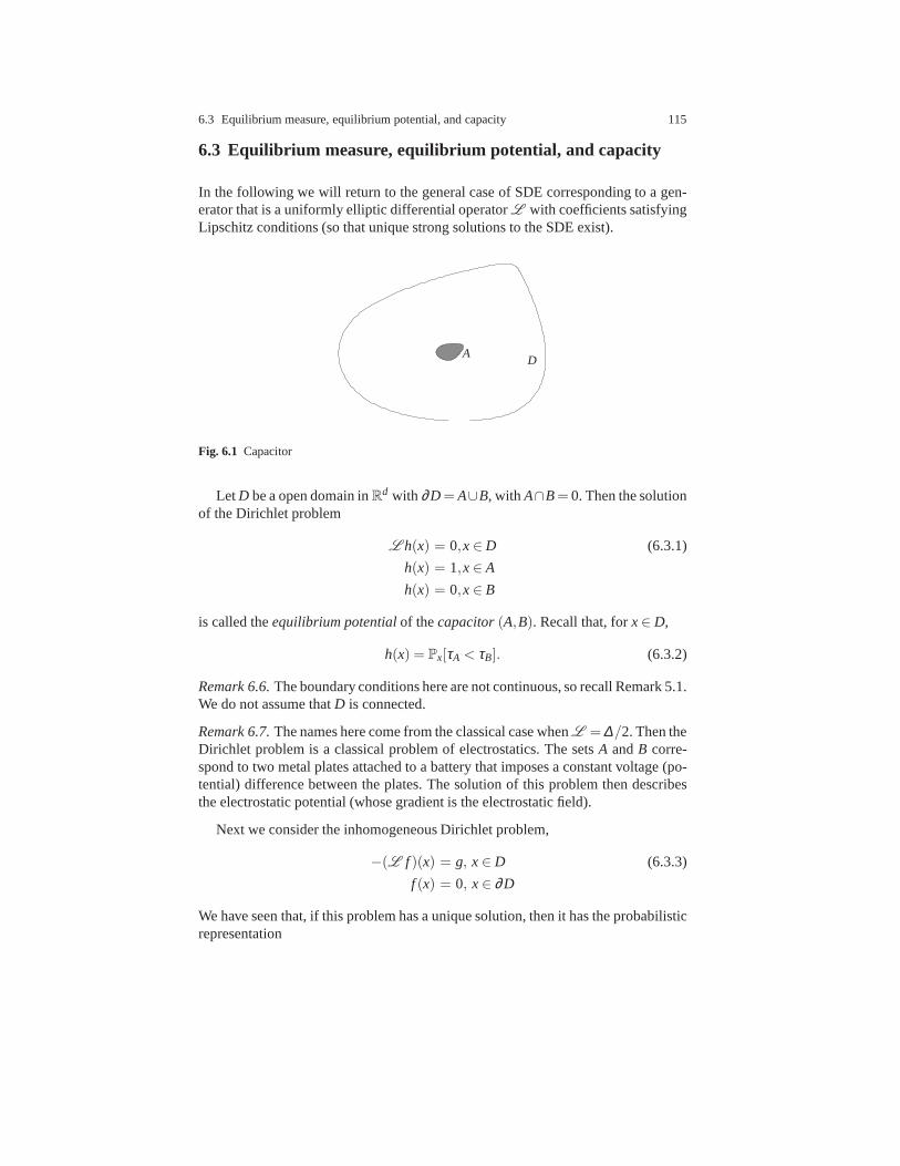
6.3 Equilibrium measure, equilibrium potential, and capacity 115

6.3 Equilibrium measure, equilibrium potential, and capacity

In the following we will return to the general case of SDE corresponding to a gen-erator that is a uniformly elliptic differential operatorL with coefficients satisfyingLipschitz conditions (so that unique strong solutions to the SDE exist).

AD

Fig. 6.1 Capacitor

LetD be a open domain inRd with ∂D=A∪B, with A∩B= 0. Then the solutionof the Dirichlet problem

L h(x) = 0,x∈ D (6.3.1)

h(x) = 1,x∈ A

h(x) = 0,x∈ B

is called theequilibrium potentialof thecapacitor(A,B). Recall that, forx∈ D,

h(x) = Px[τA < τB]. (6.3.2)

Remark 6.6.The boundary conditions here are not continuous, so recall Remark 5.1.We do not assume thatD is connected.

Remark 6.7.The names here come from the classical case whenL =∆/2. Then theDirichlet problem is a classical problem of electrostatics. The setsA andB corre-spond to two metal plates attached to a battery that imposes aconstant voltage (po-tential) difference between the plates. The solution of this problem then describesthe electrostatic potential (whose gradient is the electrostatic field).

Next we consider the inhomogeneous Dirichlet problem,

−(L f )(x) = g, x∈ D (6.3.3)

f (x) = 0, x∈ ∂D

We have seen that, if this problem has a unique solution, thenit has the probabilisticrepresentation


f (x) = Ex

∫ τD

0g(Xt) = Ex

∫ τD

0

∫

DPD

t (x,dy)g(y)dt, (6.3.4)

wherePDt (x,dy) is the sub-Markov semi-group associated to the generatorL D of

the process killed when exitingD. Thus we define theGreen kernel,

GD(x,dy)≡ Ex

∫ τD

0PD

t (x,dy)dt (6.3.5)

in terms of which the solution of (6.3.3) can be written as

f (x) =∫

Dg(y)GD(x,dy)≡ (GDg)(x). (6.3.6)

Note the similarity with theresolventof the semigroup. In fact, one may define

G(λ )D (x,dy)≡ Ex

∫ τD

0e−λ tPD

t (x,dy)dt (6.3.7)

ThenGλD exists for allλ > 0 even ifExτD = ∞, and

fλ (x) =∫

Dg(y)G(λ )

D (x,dy)≡ (G(λ )D g)(x) (6.3.8)

solves the Dirichlet problem

(−L −λ ) fλ (x) = g,x∈ D (6.3.9)

h(x) = 0,x∈ ∂D

Note that it is of course an interesting question (to which wewill return), to ask for

which values ofλ we can still defineG(λ )D for givenD.

The Green kernel will often have a density with respect to Lebesgue measure,i.e.

GD(x,dy) = GD(x,y)dy. (6.3.10)

The functionGD(x,y) is then called theGreen function.Let us now look at the relation between equilibrium potential and the Dirichlet

form in the case of a reversible diffusion. Let us try to computeE (h,h). One mightbe tempted to think thatE (h,h) = 0, sinceL h(x) = 0 except on the boundary of thesetsA andB. But of course on these,L h may be singular, since no differentiabilityassumptions are made on the boundary. So we may interpretL h as a measure thatis concentrated on the boundaries ofA andB. Sinceh vanishes on∂B, we get that

E (h,h) =−∫

∂Aµ(x)(L h)(dx). (6.3.11)

The measure(−L h)(dx) is called theequilibrium measureassociated to the capac-itor A,B.


To understand this better, let us return to the caseai j (x) ≡ δi j . We then have thefollowing integral formula, known as thefirst Green’s formula.

Theorem 6.8.Let D be a regular domain and letφ ,ψ be in C2(D). LetL be givenby (5.1.2). Then

∫

DdxeF(x)(〈∇φ(x),∇ψ(x)〉−ψ(x)(2L φ)(x)

)(6.3.12)

=

∫

∂DeF(x)ψ(x)∂n(x)φ(x)dσD(x),

where∂n(x) denotes the inner normal derivative at x∈ ∂D.

Proof. In the caseF = 0 this formula a classical. The extension to the general caseis by a straightforward computation.⊓⊔

Remark 6.9.An immediate consequence of this identity is the so-calledsecondGreen’s formula,

∫

DeF(x)dx

(φ(x)(2L ψ)(x)−ψ(x)(2L φ)(x)

)(6.3.13)

=

∫

∂DeF(x)(ψ(x)∂n(x)φ(x)−φ(x)∂n(x)ψ(x))dσD(x)

The second Green’s formula gives rise to the integral representation of a solution ofthe Dirichlet boundary value problem,

−(L f )(x) = 0, x∈ D, (6.3.14)

f (x) = u(x), x∈ ∂D,

in terms of thePoisson kernel, namely

f (x) =∫

∂DeF(y)−F(x)u(y)∂n(y)GD(y,x)dσD(y). (6.3.15)

Using the first Green’s formula, we can give a precise relation between equilib-rium potential and capacity. Namely, settingφ = ψ = h in (6.3.14), we see that

∫

DdxeF(x)〈∇h(x),∇h(x)〉=

∫

AeF(x)∂n(x)h(x)dσA(x), (6.3.16)

i.e. we have that onA the equilibrium measure,(−L h)(x) is given by

eA,B(dx)≡ ∂n(x)h(x)dσA(x). (6.3.17)

The quantity

cap(A,B)≡∫

AeF(x)∂n(x)h(x)dσA(x), (6.3.18)


is called thecapacityof the capacitorA,B. In electrical language, it is the totalcharge on the plateA. Using relation (6.3.16), we see that alternatively, the capacityis also the totalenergyof the potentialh.

Last exit distribution and equilibrium measure.

It will be nice to have a probabilistic interpretation of theequilibrium measure thatwill at the same time explain whyLh really becomes a surface measure.

We see that, forx in A, we should have something like

−(L h)(x) = limt↓0

t−1(1−Pt)(h(x)) (6.3.19)

= limt↓0

t−1Ex (1−PXt [τA < τB])

= limt↓0

t−1ExPXt [τB < τA] .

Let us define thelast exit time, LA, from A as

LA ≡ sup0< 0< τB : Xt ∈ A, (6.3.20)

with the convention sup /0= 0 Note that this is obviously no stopping time and that

Px[LA > 0] = Px[τA < τB]≡ h(x). (6.3.21)

Note that we can write the expression in the last line of (6.3.19) as

ExPXt [τB < τA] = Px[0< LA < t].

Hence we setψt(z)≡ t−1Pz[0< LA < t] . (6.3.22)

Let us also define thelast exit distribution, L(x,dy), onA, by

L(x,dy) ≡ Px [XLA− ∈ dy;LA > 0] . (6.3.23)

We want to prove the following lemma:

Lemma 6.10.Let f be a continuous function onD. Then

limt↓0

∫GD(x,y)ψt(y) f (y)dy=

∫

AL(x,dy) f (y). (6.3.24)

Proof. Without loss let f ≥ 0. Using the representation of the Green functionthrough the semigroup (6.3.5) we get


∫GD(x,y)ψt(y) f (y)dy = Ex

∫ τB

0ψt(Xs) f (Xs)ds (6.3.25)

= t−1∫ ∞

0Ex [ f (Xs)PXs[0< L < t]]ds

= t−1∫ ∞

0Ex [ f (Xs)1Is<L<s+t ]ds

= Ex

[0< LA ≤ t; t−1

∫ La

0f (Xs)ds

]

+Ex

[t < LA; t−1

∫ La

LA−tf (Xs)ds

].

First, both terms in the last line are obviously uniformly bounded ast ↓ 0. Moreover,

Ex

[0< LA ≤ t; t−1

∫ La

0f (Xs)ds

]≤CEx [0< LA ≤ t] ↓ 0, (6.3.26)

ast ↓ 0. Finally, by continuity off ,

limt↓0

Ex

[t < LA; t−1

∫ La

LA−tf (Xs)ds

]= Ex [0< LA; f (XLA−)ds] . (6.3.27)

Integrating overA gives the claim of the lemma.⊓⊔

From Lemma (6.10) one can deduce that the family of measuresψt(y)dy con-verges to a measuree(dy) onA. Moreover, this measure satisfies

GD(x,y)e(dy) = L(x,dy). (6.3.28)

Integrating this formula overA, we arrive at the expression∫

AGD(x,y)e(dy) =

∫

AL(x,dy) = h(x). (6.3.29)

Hencee(dy) satisfies the defining relation of the equilibrium measureThus we have proven a very interesting and useful relation between the equilib-

rium potential, the equilibrium measure, and the Green function.

Theorem 6.11.Let as before A⊂ D be open sets with smooth boundary. Then, forall x ∈ D,

h(x) =∫

∂AGD(x,y)eA,D(dy). (6.3.30)

Remark 6.12.Is is instructive to think about this result in the followingway. Wehave already seen that we may want to think ofL h as a measure. Then we havethat

−(L h)(x)dx= eA,D(dx), x∈ D, (6.3.31)

h(x) = 0, x∈ ∂D.


Then the solution of this problem in terms of the Green function is precisely theexpression (6.3.30). Note that (6.11) holds also inA, with h(x) = 1.

This formula for the Green function gives of course corresponding formulas forsolutions of Dirichlet problems. E.g., if we consider for some functiong the Dirich-let problem

−(L f )(x) = g(x), x∈ D (6.3.32)

f (x) = 0, x∈ ∂D,

then of coursef (x)=∫

D dyGD(x,y)g(y). By symmetry,GD(x,y)= eF(y)−F(x)GD(y,x),and so

∫

DdxeF(x)h(x)g(x) =

∫

Ddxh(x)

∫

∂AeF(x)g(x)GD(y,x)e

F(y)−F(x)eA,D(dy)

=∫

∂AeF(y)

∫

DGD(y,g)g(x)eA,D(dy)

=

∫

∂AeF(y) f (y)eA,D(dy). (6.3.33)

Introducing the probability measure

νA,D(dy)≡ eF(y)eA,D(dy)cap(A,D)

, (6.3.34)

on ∂A, this gives

∫

∂AνA,D(dy) f (y) =

1cap(A,D)

∫

DdxeF(x)h(x)g(x). (6.3.35)

As a particular example we get, withg(x) = 1,

∫

∂AνA,D(dy)EyτD =

1cap(A,D)

∫

DdxeF(x)h(x). (6.3.36)

Dirichlet principle

. We have seen that the equilibrium Dirichlet form computed on the equilibriumpotential gives the capacity. We will how show that the equilibrium potential is thesolution of a variational problem.

Theorem 6.13.With the notations and assumptions above, the following holds. LetHA,B be the space of continuous functions„ f , onD such that,

(i) E ( f , f ,) < ∞, and(ii) f (x)≥ 1, x∈ A and f(x) ≤ 0, x∈< Dc.

6.4 The case of dimension one. 121

cap(A,B) = inff∈HA,B

E ( f , f ). (6.3.37)

Moreover, ifHA,B 6= /0, the infimum in (6.3.37) is achieved uniquely on the equilib-rium potential, i.e.cap(A,B) = E (hA,B,hA,B).

Proof. Let us assume that the setHA,B is not empty. Consider a functiong such thatE (g,g)< ∞ and thatg vanishes on both∂B and∂A. Notice that, forh∈ HA,B,

E (h+εg,h+εg)−E (h,h) = 2ε∫

D\A∪Bµ(dx)g(x)(L h)(x)+ε2

E (g,g). (6.3.38)

This implies two things: first, ifL h(x) = 0, thenh is a global minimum ofE inHA,B. We know already that such a function exists, namely the equilibrium poten-tial. Next assume that there is another function,f , such thatE ( f , f )) = E (h,h).Then the identity

E

(f+h2 , f+h

2

)+E

(f−h2 , f−h

2

)=

12E ( f , f )+

12E (h,h), (6.3.39)

implies that

E

(f+h2 , f+h

2

)≤ E (h,h)−E

(f−h2 , f−h

2

). (6.3.40)

Sinceh is an absolute minimum, this can only hold if

E ( f −h, f −h) = 0. (6.3.41)

But this means that‖∇( f −g)(x)‖2 = 0 µ-almost surely. ⊓⊔

The Dirichlet principle is a powerful tool for asymptotic computations of capaci-ties, and, hence, as we shall see, much more. To a large extendthis is due to the factthat it allows for natural upper and lower bounds. The most immediate one of theseis of course given by the elementary observation that

Corollary 6.14. For any function, f∈ HA,B,

cap(A,B)≤ E ( f , f ). (6.3.42)

6.4 The case of dimension one.

The above considerations lead to very explicite answers in the case whend = 1.The first observation is that all homogeneous boundary valueproblems in this casecan, by linearity, be reduced to computing the equilibrium potential for on interval(a,b),i.e.


(L h)(x) = 0, x∈ (a,b) (6.4.1)

h(a) = 0

h(b) = 1

Note also that the general uniformly elliptic case, we can bereduced to the problemwith generator

(L h)(x) =−12

f ′′(x)+b(x) f ′(x). (6.4.2)

Note also that, ind = 1, any bounded functionb can be written as a derivative ofanother function,F/2, where

F(x) = 2∫ x

0b(x)dx. (6.4.3)

-3 -2 -1 1 2 3

0.5

1.0

1.5

2.0

2.5

Fig. 6.2 A potential function on[−3,3]

Thus we are always in the reversible case. Hence we are reduced to solving theordinary differential equation

12

h′′(x)+b(x)h′(x) = 0, (6.4.4)

which in turn reduces to the first order equation

12

u′(x)+b(x)u(x) = 0 (6.4.5)

when we setu= h′. Clearly (6.4.5) has the general solution

u(x) =C1e−F(x) (6.4.6)

and so the general solution of (6.4.4) is

6.4 The case of dimension one. 123

50 100 150 200 250 300

0.2

0.4

0.6

0.8

1.0

Fig. 6.3 The corresponding equilibrium potentialPx[τ3 < τ−3]

h(x) =C1

∫ x

0e−F(y)dy+C2, (6.4.7)

with C1 andC2 integration constants to be determined from the boundary conditions.In particular, for the equilibrium potential related to theinterval(a,b) we have

h(x) =

∫ xa e−F(y)dy∫ b

a e−F(y)dy. (6.4.8)

Hence the capacity cap(a,b) is readily computed as

cap(a,b) = E (h,h) =1

2∫ b

a e−F(y)dy. (6.4.9)

Some reflection shows that we can get from (6.11) the following formula for theGreen function in(a,b): Forx< y,

G(a,b)(x,y) =hx,a,b(y)

ex,b(6.4.10)

= F(x) 1−hx,b(y)

cap(x,b)

= eF(x)

∫ by e−F(z)dz∫ bx e−F(z)dz

12∫ bx e−F(z)dz

=12

eF(x)∫ b

ye−F(z)dz

and fory< x,

G(a,b)(x,y) =12

eF(y)∫ y

ae−F(z)dz. (6.4.11)


6.5 Another view on one-dimensional diffusions

We have seen in the previous section that the computation of the equilibrium po-tential in one-dimensional case allows to compute the Greenfunction and hence toessentially solve everything that can be expressed in termsof Dirichlet problems.

We will now take a different look at the same issue. The perspective will bemore on the level of the process. We will see that the solutionof a 1d SDE can beconstructed from Brownian motion in a way that will exhibit again the crucial rôle.

Let us recall that the harmonic functions we encountered canbe written in theform

Px(τa < τb) =s(x)− s(a)s(b)− s(a)

, (6.5.1)

wheres(x) is an increasing function whose derivative ise−F(x). The functions isusually called thescale functionRecall that in the case of Brownian motion,s(x) =x. Now letB be Brownian motion and consider the processYt = s−1(Bt). Clearly wehave that

PYx (τa < τb) = PB

s(x)(τs(a) < τs(b)) =s(x)− s(a)s(b)− s(a)

, (6.5.2)

(here the superscripts indicate that the probabilities arew.r.t. the correspondingprocesses) hence the process has the same harmonic functionas the one solvingdXt =

12F ′(Xt)dt+dBt . Is it the same process? No, but using Itô’s formula, we see

thatZt ≡ s(Xt) satisfies

dZt = s′(Xt)dXt +12

s′′(Xt)dt (6.5.3)

= s′(Xt)dBt +12(s′(Xt)F

′(Xt)+ s′′(Xt))dt

= s′(s−1(Xt)

)dBt ,

which is of the formdZt = g(Zt)dBt . (6.5.4)

We will show that any solution of an SDE of the form (6.5.4) is atime change ofBrownian motion.

Theorem 6.15.Let g be a measurable function such that g(x)≥ δ > 0. Then (6.5.4)has a unique weak solution. Moreover, there exists a Brownian motion, B, such that

Zt = B(γt), (6.5.5)

whereγt ≡ infu : A(u)> t, and

A(t)≡∫ t

0g(B(u)−2du. (6.5.6)

Proof. Clearly we have that th ifZ solves (6.5.4), then

6.5 Another view on one-dimensional diffusions 125

d[Z]t = g(Zt)2dt. (6.5.7)

On the other hand,[B][Z]t = [Z]t . (6.5.8)

Inverting this relation we may write

B(t) = Zτ(t), (6.5.9)

whereτ(t) is the inverse time change, i.e.

[Z]τ(t) =∫ τ(t)

0g(Zu)

2du= t. (6.5.10)

Differentiating this latter relation we get

1= g(Zτ(t))2τ ′(t) = g(B(t))2τ ′(t). (6.5.11)

Hence

τ ′(t) =1

g(B(t))2 , (6.5.12)

and hence

τ(t) =∫ t

0

1g(B(u))2du, (6.5.13)

τ being the inverse of the time change, we see that the time change[Z]t is really theinverse of the functionτ, which is given purely in terms of the Brownian motionB.⊓⊔

It remains to generalize the first part of our construction. Thus consider the gen-eral form of the SDE

dXt = b(Xt)dt+σ(Xt)dBt , (6.5.14)

with σ > 0. We know already that the equilibrium potential will be of the form(6.5.1) withs being an integral of

s′(x) = e−∫ x0 2b(z)/σ2(z)dz. (6.5.15)

AgainZt = s(Xt) then has the same harmonic function as Brownian motion, and thesame calculation as in (6.5.3) shows thatZt is a solution of (6.5.4), this time with

g(x) = s′(s−1(x))σ(s−1(x)). (6.5.16)

We summarize these results in the following theorem.

Theorem 6.16.Assume thatσ(x)> 0, as long as∫ x

0 b(z)σ−2(z)<∞ exists for x∈ I,then the SDE has a unique weak solution given by

Xt = s−1 (B(γt)) , (6.5.17)


whereγt is the continuous inverse of the function

At ≡∫ t

0

1g(B(u))2du, (6.5.18)

where g is given by (6.5.16), and B is Brownian motion.

The strong point of this result is that very little regularity is required for thedrift or difussivity. For example, this theorem allows to make sense of theBrownianmotion in a Brownian potential: Let W(t) be a realization of a Brownian motion,and consider the formal expression

dXt =W′(Xt)dt+dBt . (6.5.19)

SinceW is not differentiable, this expression is formal. However,the correspondingpotential,W, is well defined, and so is the scale functions(x) = exp(W(x)). Thuswe can interpret the process obtained from Eqs. (6.5.17)-(6.5.18) as the solution of(6.5.19).

6.6 Brownian local time and speed measures

The aim of this section is to give an alternative representation of the time changeformula that will give rise to the possibility to construct even larger classes of onedimensional diffusion processes. At the same time we will deepen the discussionof local timethat was initiated in Theorem 4.9. The following discussiondraws onlecture notes by Steve Lalley.

Let us first observe what would be the natural notion of a occupation measure.Let A∈ B(R) be a Borel subset of the real line. Then we can introduce

Γt(A)≡∫ t

01IA(Bs)ds (6.6.1)

as a random measure on(R,B(R)). The main result we will use and need, is thefollowing theorem.

Theorem 6.17.With probability one, for each t< ∞, the occupation measureΓt isabsolutely continuous with respect to Lebesgue measure, and it density, lxt , is jointlycontinuous in t and x.

lxt is called thelocal timeof Brownian motion atx. We have already seen that thelocal time at zero can be represented as a stochastic integral via an extension of Itô’sformula (Tanaka’s formula). This gives the representation

lat ≡ |Bt −a|− |B0−a|−∫ t

0sign(Bs−a)dBs. (6.6.2)

We will first show that

6.6 Brownian local time and speed measures 127

Theorem 6.18.There exists a version of the processlat ,a ∈ R, t ∈ R+ that isjointly continuous in t and a.

Proof. We will deal with a fixed time horizonT < ∞. Define

ξ1(a, t)≡∫ t

0sign(Bs−a)dBs (6.6.3)

andξ2(a, t)≡ |Bt −a|− |B0−a|. (6.6.4)

Obviouslyξ2 is jointly continuous, sinceB is continuous. Thus we need to provethat ξ1 has a jointly continuous version. The tool to prove this is a lemma due toKolmogorov.

Lemma 6.19.Letξ be a stochastic process indexed byRn with values in a completemetric space with metricρ . If there exist positive constants,α,β ,ε, such that

E(ρ(ξx,ξy))α ≤ β |x− y|n+ε , (6.6.5)

for all x,y∈Rn, then there exists a continuous version of X.

We apply this theorem to the processξ1(·, t), t ∈ [0,T]. We may also consider theprocess on a bounded interval. Then it will be enough to show that

E |ξ1(x, t)− ξ1(y, t)|p ≤ C|x− y|2+δ (6.6.6)

E∣∣ξ1(x, t)− ξ1(x, t

′)∣∣p ≤ C|t − t ′|2+δ

Now

|ξ1(x, t)− ξ1(y, t)| =∣∣∣∣∫ t

0(sign(Bs−a)− sign(Bs−b))dBs

∣∣∣∣

≤ 2∫ t

01I(x,y)(Bs)dBs. (6.6.7)

Hence, using the Burkholder inequalities,

E |ξ1(x, t)− ξ1(y, t)|2m ≤ 22mE

∣∣∣∣∫ t

01I(x,y)(Bs)dBs

∣∣∣∣2m

(6.6.8)

≤ Cm22mE

∣∣∣∣∫ t

01I(x,y)(Bs)ds

∣∣∣∣2m

.

In the final expression we can now estimate


E

∣∣∣∣∫ t

01I(x,y)(Bs)ds

∣∣∣∣2m

(6.6.9)

= m!∫

0≤t1≤tm−1≤···≤tm≤tP [Bt1 ∈ (x,y), . . . ,Btm ∈ (x,y)]

≤ m!∫

0≤t1≤tm−1≤···≤tm≤tE

[PB0(Bt1 ∈ (x,y)]PBt1

(Bt2 ∈ (x,y)) . . .

. . .PBtm−1(Btm∈ (x,y))

]

≤ m!(y− x)m√

tm.

The corresponding estimate for different times is similar.⊓⊔

With this absolutely continuous local time process we can ofcourse write thetime change function (6.5.18) in the form

At =

∫ t

0

1g(Bu)2 du=

∫dx

1g(x)2

∫ t

0δBu(x)du=

∫m(dz)lzt , (6.6.10)

wherem(dz) = g−2(z)dz and lzt is the density of the Brownian local time process.The measurem(z) is called hespeed measure(essentially it tells us how the localtime of Brownian motion is transformed to the time of the new process in the pointz). . This formulation gives rise to an even wider class of one-dimensional diffusionsthat can be constructed as time changes of Brownian motion through more generalspeed measures. Note that these processes are all Markovian, which is not a trivialfact (see [15], Chapter III.21 and [14], Chapter V.47).

6.7 The one-dimensional trap model and a singular diffusion

In the following we show that these processes are not totallyhypothetical, but thatthey can arise from more or less reasonable discrete models.

In the following we will give the construction of a random motion in a randomenvironment that was studied by Fontes, Isopi, and Newman some years ago [7].

We begin be prescribing a random environment onZ as a family of iid randomvariables,τi , i ∈ Z, whose distribution will be be assumed to satisfy

limt↑∞

tαP[τ1 > t] = 1 (6.7.1)

for α < 1. Note that this implies in particular thatEτ1 = +∞. Our next ingredientwill be a continuous time, unbiased simple random walk,Zk, k∈ N, onZ.

(Note that a continuous time random walk can be described as follows: LetYk,k ∈ N, be a discrete time simple random walk onZ (i.e.Yk = ∑k

i=1ui , whereui areiid with P[ui = ±1] = 1

2). Let C(k) = ∑k−1i=0 ei , whereei , i ∈ N, are iid exponential

random variables with rate 1. Then

6.7 The one-dimensional trap model and a singular diffusion 129

Zt =YC−1(t) (6.7.2)

whereC−1 is the inverse ofC,

f−1(t) = infk : f (k) > t. (6.7.3)

We will now construct a continuous time process a time changeof the simpleradom walkZ as follows. Define the so-calledclock process

S(u)≡∫ u

0τZr dr (6.7.4)

The processX is then defined, for a given realization of the random variablesτi , as

Xt = ZS−1(u) (6.7.5)

We now want to re-write the clock process in terms of a speed measure. For this wedefine the local time process ofZ as

L( j, t) =∫ t

01IZu= jdu. (6.7.6)

Then we can re-write the clock process as

S(u) = ∑j∈Z

τ j L( j,u). (6.7.7)

One sees easily that there is a complete analogy between the construction of a dif-fusion from Brownian motion.

We now consider a rescaling of space and time to obtain a continuous processlimit. Clearly we have from (a complete analog of) Donsker’sinvariance principlethat

limε↓0

εZt/ε2 = Bt . (6.7.8)

Now assume that for someβ ,

ε2S−1(ε−β t)≡ S−1ε (t)→ Σ−1(t), (6.7.9)

thenXε

t ≡ εXε−β t = εZε−2S−1ε (t) ≡ Zε

S−1ε (t)

(6.7.10)

and we may expect thatZε

S−1ε (t)

→ BΣ−1(t). (6.7.11)

The question is thus to see whether and to what the processε2S−1(ε−β t), respec-tively its inverse,

Sε(u)≡ εβ S(u/ε2), (6.7.12)

converges. Now


εβ S(u/ε2) = ∑i∈Z

εβ τiL(i,u/ε2)≡ ∑i∈Z

εβ τiLε(ε i,u), (6.7.13)

where by definitionLε (ε i,u) = L(i,u/ε2).We may expect this to converge to thelocal time process of Brownian motion. On the other hand, we can think of the sumas an integral over the random measure

mε(dx)≡ ∑i∈Z

δiε(dx)τiεβ , (6.7.14)

i.e.Sε(t) =

∫mε(dx)Lε (x, t), (6.7.15)

It is a curious fact that in distribution,∫

mε(dx)Lε (x, t) =∫

mε(dx)lxt (6.7.16)

This is due to the fact that the local time density of Brownianmotion on an integerpoint i before visiting one of its neighbors is an exponential random variable withmean one. To see this, observe that the continuous time simple random walk onZcan be coupled to a Brownian motion: consider the measurem0(dx) ≡ ∑i∈Z δi(dx)as a speed measure and letYt be the time change of a Brownian motionBt with thisspeed measure. This is a Markov process that spends all of itstime on the integersand jumps with infinite speed between them. It is clear that this process visits thesites i ± 1 with equal probability afteri. Moreover, form the fact that the processobserved on the sitesi is Markov, the waiting time ati before the process reachesi ±1 is exponential. Its mean value is given byE0ℓ

0τ1∧τ−1

. Using Tanaka’s formulafor the local time of Brownian motion, we get

E0ℓ0τ1∧τ−1

= E0∣∣Bτ1∧τ−1

∣∣= 1. (6.7.17)

Thus we see that we have indeed a relisation of the processY as timechange ofBrownian motion.

Thus we have actually immediately an expression of our (rescaled) processXε

immediately as a time change of Brownian motion with speed measuremε .Thus the key question is whethermε(dx) converges. this will be the case, due to

(6.7.1), ifβ = 1/α. This follows from a more general result about the convergenceof so-called extremal processes.

(for a proof see, e.g., [13]):

Theorem 6.20.Assume that Xi are iid random variables that satisfy

limn↑∞

ε−1P[Xi > uε(c)] = ν(c). (6.7.18)

whereν is an increasing (respectively decreasing) function. Then, the point process

∑i∈Z

δ(iε,u−1ε (Xi))

(6.7.19)


converges in distribution to the Poisson point process,R onR+×R with intensitymeasure dt×dν(x) (respectively−dν if ν is decreasing).

Using the property (6.7.1), we see that in our case, withuε(c)≡ ε−1/αc, we havethat

ε−1P[τ1 > ε−1/αc] = c−α [ε−1/αc]αP[τ1 > ε−1/αc]→ c−α .

Thus the theorem yields

Corollary 6.21. The point process

Rε ≡ ∑i∈Z

δ(iε,ε1/α τi)→ R (6.7.20)

converges to the Poisson point process onR×R+ with intensity measure dt×αc−1−αdc.

One can show that this implies that, ifα < 1, the measures

mε(dx) =∫

Rε(dx,dt)t (6.7.21)

converge to the measure

m(dx)≡∫

R(dx,dt)t. (6.7.22)

Note of course that we are speaking of random measures here. So what convergesis the distribution of these random measures. In proper terms, we would have toequip the space of measures with a topology (e.g. the vague topology) and speak ofweak convergenceof the family of random measures with respect to this underlyingtopology.

One can easily check that the measurem(dx) is singular (in fact it is a purepoint measure) with respect to Lebesgue’s measure. Nonetheless one can use it toconstruct a singular diffusion as a time change of Brownian motion form it, that willbe the natural candidate for the limit process in our model.

It is known that if a sequence of (point) measures,νn, converges to a point mea-sureν (in a suitable topology that I will not discuss here), then the correspondingtime-changed processes converge to the process with time change obtained from thespeed measureν.

Can we apply this fact in our case, when the measuresµε converge only inweakly? The answer is yes, in general due to Skorohod’s theorem, that states thatweak convergence of a family of random variables,Xn, is equivalent to the existenceof a another family,Xn, such that for eachn, Xn andXn have the same distribution,while Xn converges almost surely.


A coupling

. It is an amusing observation that in the case of our random measuresmε , thisconstruction can be made in a very explicit way. It will also exhibit a deep relationbetween these measures and Lévy processes.

Let us first briefly recall what anα-stable Lévy subordinator,U , is. There arein fact at least two ways to describe it: one is to say thatU is a non-decreasingstationary process with independent increments whose Laplace transform is givenby

Ee−λU(x) = exp

[xα∫ ∞

0(e−λ w−1)w−1−αdw

]. (6.7.23)

Another way to characterize it is to say that it is the distribution function onRassociated with the measurem(dx), normalized s.t.U(0) = 0 (see my lecture noteson ageing [2]).

Now introduce the scaling functionG such that

P[U(1)≤ G(a)] = P[τ0 ≤ a]. (6.7.24)

Then defineτε

i ≡ G−1(

ε−1/α (U(ε(i +1)−U(ε i))). (6.7.25)

Lemma 6.22.The family of random variablesτεi , i ∈ Z is iid andτε

i has the samedistribution asτ1.

Proof. The proof of this lemma follows form the fact that the subordinatorU isα-stable, i.e. thatε−1/αU(ε) has the same law asU(1). ⊓⊔

Using these random variables we can construct measures

mε ≡ ∑i∈Z

ε1/α τεi δε i , (6.7.26)

which now converge almost surely tom, where of course the the distribution func-tion of thism is used asU in the construction of theτε

i . In the case whenG is theidentity, this is quite straightforward, whereas in the general case some care is re-quired to show this fact (see [7]). The key is that by the assumptions on the law ofτi , G is close to linear at infinity and soε1/αG−1(ε−1/αx)→ x, asε ↓ ∞.

The existence of a non-trivial scaling limit for this model have far-reaching con-sequences for its long time asymptotics. In particular, it implies so-calledagingbehavior. This notion refers to the long-time behavior of of certaincorrelation func-tionsof the process, e.g.

R(tw, t)≡ P[Xt+tw = Xtw]. (6.7.27)

One says that a process shows aging, if

limtw↑∞

R(tw,θ t) = f (θ ), (6.7.28)


for some non-trivial functionf . Now in our case we have that

R(tw,θ t) = P[Xtw(1+θ = Xtw] = P[Xt−1/αw

1+θ = Xt−1/αw

1 ]. (6.7.29)

Again we may expect this to converge to

P[BΣ(1+θ) = BΣ(1)

], (6.7.30)

which would be our desiredageing functionexpressed in term of the limiting pro-cess.

Chapter 7Appendix: Weak convergence

In this short section we collect some necessary material forunderstanding the con-vergence of sequences of stochastic processes with path properties. This will allowus to put the analysis of the Donsker theorem into a general framework.

7.1 Some topology

We consider the general setup on a compact Hausdorff space,J. We denote byC(J)the Banach space of bounded, continuous real-valued functions equipped with thesupremum norm. We denote byM1(J) the space of probability measures onJ. Wedenote byC(J)∗ the space of bounded linear functionalsC(J)→R onC(J).

We need two basic facts from functional analysis:

Theorem 7.1.[Stone-Weierstrass theorem]Let A be a sub-algebra of C(J) that con-tains constant functions and separates points of J, i.e. forany x∈ J there exitsf ,g∈ A such that f(x) 6= g(x). Then A is dense in C(J).

Theorem 7.2.[Riesz representation theorem]Let φ be a positive linear functionalφ : C(J) → R with Φ(1) = 1. Then there exists a unique inner regular probabilitymeasure,µ ∈ M1(J), such that

φ( f ) = µ( f ) =∫

Jf dµ . (7.1.1)

Recall (see [1] page 12) that a measure isinner regular, if for any Borel set,B,µ(B) = supµ(K),K ⊂ B, compact. We have shown there already, that ifJ is acompact metrisable space, then any probability measure on it is inner regular.

The weak-∗ topology on the spaceC(J)∗ is obtained by choosing sets of the form

Bf1,..., fn,ε(φ0)≡ φ ∈C(J)∗ : ∀1≤i≤n|φ( fi)−φ0( fi)|< ε (7.1.2)

135

136 7 Appendix: Weak convergence

with n ∈ N,ε > 0, fi ∈ C(J) as a basis of neighborhoods. The ensuing space is aHausdorff space.

When speaking of convergence on topological spaces, it is useful to extend thenotion of convergence of sequences to that ofnets.

Definition 7.3. A directed set, D, is a partially ordered set all of whose finite subsetshave an upper bound inD. A net is a family(xα ,α ∈ D) indexed by a directed set.

If (xα ,α ∈ D) is a net in a topological space,E, thenxa → x if, for every openneighborhood,G, of x, there existsa0 ∈ D such that for allα ≥ α0, xα ∈ G.

Lemma 7.4.A netφα in C(J)∗ converges in the weak-* topology to some element,φ , if and only if, for all f ∈C(J), φα( f )→ φ( f ).

Proof. Let us prove first the “if” part. Then for anyf , and anyε, there existsα f , such that for allα ≥ α f , φα( f )− φ( f )| < ε. Now take any neighborhoodBf1,..., fn,ε(φ). Then, letα0 ≡ maxn

i=1α fi , and it follows thatφα ∈ Bf1,..., fn,ε(φ), forα ≥ α0, henceφa → φ . For the converse, we have that for anyn∈N, any collectionf1, . . . , fn, and anyε > 0, there existsα0 such that, ifφα0 ∈ Bf1,..., fn,ε (φ), then forall α ≥ α0, φα ∈ Bf1,..., fn,ε (φ). Thus to show that for any givenf , φα( f ) → φ( f )we just have to use this fact withBf ,ε(φ).

One of the most important facts about the weak-∗ topology is Alaoglu’s theo-rem. The spaceC(J)∗ is in fact a Banach space equipped with the norm‖φ‖ ≡supf∈C(J)

φ( f )‖ f‖∞

Theorem 7.5.The unit ball

φ ∈C(J)∗ : ‖φ‖ ≤ 1 (7.1.3)

is compact in the weak-∗ topology.

(for a proof, see any textbook on functional analysis, e.g. Dunford and Schwartz[5]).

The importance for us is that when combined with the Riesz representation the-orem, it yields:

Corollary 7.6. The set of inner regular probability measures on a compact Haus-dorff space is compact in the weak-∗ topology.

Proof. By the Riesz representation theorem, each inner regular probability measurecorresponds to a unique increasing functional,φ ∈C(J)∗ with φ(1) = 1. Since thefunction f ≡ 1 is the largest function such that‖ f‖∞ ≤ 1, it follows that‖φ‖ ≤φ(1) = 1. Hence this set is a subset of the unit ball. Moreover, the set of increasing(in the sense of non-decreasing) linear functionals mapping 1 to 1 is closed, andhence, as a closed subset of a compact set, compact.

Corollary 7.7. The set of probability measures on a compact metrisable space iscompact in the weak-∗ topology.

7.2 Polish and Lousin spaces 137

Proof. By Theorem 1.2.6 in [1], any probability measure on a compactmetrisablespace is inner regular, hence the restriction to inner regular measures in Corollary7.6 can be dropped in this case.

As a matter of fact, in the compact metrisable case we get evenmore.

Theorem 7.8.Let J be a compact metrisable space. Then C(J) is separable, andM1(J) equipped with the weak-∗ topology is compact metrisable.

Proof. We may takeJ to be metric with metricρ . SinceJ is separable (any compactmetric space is separable), there is a countable dense set ofpoints,xn, n∈N. Definethe functions

hn(x)≡ ρ(x,xn).

The functionshn separate points inJ, i.e. if x 6= y, then there existsn such thathn(x) 6= hn(y). Now letA be the set of all functions of the form

q1I+ ∑n1,...,nr ;k1,...,kr

q(n1, . . . ,nr ;k1, . . . ,kr)hk1n1. . .hkr

nr

where allq’s are rational. Then the closure ofA is an algebra containing all con-stant functions and separating points inJ. The Stone-Weierstrass theorem assertstherefore that the countable setA is dense inC(J), soC(J) is separable.

Now let fn, n ∈ N, be a countable dense subset ofC(J). Consider the mapΦ :M1(J)→V ≡×n∈N[−‖ fn‖∞,‖ fn‖∞], given by

Φ(µ) = (µ( f1),µ( f2), . . . ).

This map is one to one. Namely, assume thatµ 6= ν, butΦ(µ) = Φ(ν). Then on theone hand, there must existsf ∈C(J) such thatµ( f ) 6= ν( f ), while for alln, µ( fn) =ν( fn). But there are sequencesfi ∈ A such thatfi → f . Thus limi µ( fi) = lim i ν( fi),and by dominated convergence, both limits equalµ( f ), resp.ν( f ), which must beequal contrary to the assumption. Moreover, the setA determines convergence, i.e.a netµα converges toµ (in the weak-∗ topology , ifµα( fn)→ µ( fn), for all fn ∈ A.But the product spaceV is compact and metrisable (by Tychonoff’s theorem), andfrom the above,M1(J) is homeomorphic to a compact subset of this space. Thus itis compact and metrisable.

Let us remark that a metric onM1(J) can be defined by

ρ(µ ,ν)≡∞

∑n=1

2−n(

1−e−|µ( fn)−ν( fn)|). (7.1.4)

7.2 Polish and Lousin spaces

When dealing with stochastic processes, an obviously important space is that ofcontinuous, real valued functions onR+. We will call


W ≡C([0,∞),R). (7.2.1)

This space is not compact, so we have to go slightly beyond theprevious setting.

Lemma 7.9.The space W equipped with the topology of uniform convergence oncompact sets is a Polish space. Theσ -algebra,A , of cylinders generated by theprojectionsπt : W →R, πt(w) = w(t), is the Borel-σ -algebra on W.

Proof. We can metrise the topology onW by the metric

ρ(w1,w2)≡∞

∑n=1

2−n ρn(w1,w2)

1+ρn(w1,w2),

whereρn(w1,w2)≡ sup

0≤t≤n|w1(t)−w2(t)|.

Then it inherits its properties form the metric spaceC([0,n),R) equipped with theuniform topology.

Now the mapsπt are continuous, and henceA ⊂ B(W). On the other hand, forcontinuous functions,wi ,

ρn(w1,w2) = supq∈Q∩[0,n]

|w1(q)−w2(q)|,

so thatρn and henceρ areA -measurable. Now letF be a closed subset ofW. Takea countable dense subset ofF , saywn,n∈ N. Then

F = w∈W : infn

ρ(w,wn) = 0,

which (since all is countable) implies thatF ∈ A , and thusA = B(W).

This (and the fact that quite similarly the corresponding spaces of càdlàg functionsare Polish) implies that we can most of the time assume that wewill be working onPolish probability spaces. In the construction of stochastic processes we have actu-ally been working on Lousin spaces (and used the fact that these are homeomorphicto a Borel subset of a compact metric space). The next theoremnicely clarifies thatPolish spaces are even better.

Theorem 7.10.A topological space is Polish, if and only if it is homeomorphic to aGδ subset (i.e. a countable intersection of open subsets) of a compact metric space.In particular, every Polish space is a Lousin space.

Proof. We really only care about the “only if” part and only give its proof. LetSbeour Polish space. We will actually show that it can be embedded in aGδ subset ofthe compact metrisable spaceJ ≡ [0,1]N. Let ρ be a metric onS, and setρ = ρ

1+ρ .This is an equivalent metric that is bounded by 1. Chose a countable dense subsetxn, n∈ N, of Sand define


α(x)≡ (ρ(x,x1), ρ(x,x2), . . . ).

Let us show thatα is a homeomorphism fromS to its image,α(S) ⊂ [0,1]N. Forthis we must show that a sequence of elementsx(n) converges tox, if and only if

ρ(x(n),xk)→ ρ(x,xk),

for all k. The only if direction foillow from the continuity of the mapρ(·,xk). Toshow the other direction, note that by the triangle inequality

ρ(x(n),x) ≤ ρ(x(n),xk)+ ρ(xk,x).

Therefore, for allk,limsupρ(x(n),x) ≤ 2ρ(xk,x). (7.2.2)

Now take a sequence ofxk that converges tox. Then (7.2.2) implies that limsupρ(x(n),x)≤0, and sox(n)→, as desired.

Next, letd be a metric onJ. By continuity of the inverse mapα−1 on the imageof S, for anyn∈ N we can find 1/2n≥ δ > 0, such that the pre-image of the ballBd(α(x),δ )∩α(S) has diameter smaller than 1/n (with respect to the metricρ).

Now think ofα(S) as a subset ofJ. Let α(S) be its closure. Forn given, letUn bethe union of all pointsx∈ α(S) such that it has a neighborhood,Nn,x in J such thatα−1(Nn,x∩α(S)) hasρ-diameter at most 1/n. Note that by what we just showed,all points inα(S) belong toUn. Now we show thatUn is open inα(S): if x ∈ Un,andy∈ α(S) is close enough tox, theny∈ Nn,x, and the setNn,x may serve asNn,y,so thaty∈Un. ThusUn is open.

Now let x ∈ ⋂nUn. Choose for anyn a point xn ∈ α(S) ∩⋂k≤n Nk,x. Clearlyd(x,xn) ≤ 1/n and hencexn → x. Moreover, for anyr ≥ n, both xr ∈ Nn,x andxn ∈ Nn,x, so thatρ(α−1(xr),α−1(xn)) ≤ 1/n. Thusα−1(xn) is a Cauchy sequencein complete metric space, and soα−1(xn) → y∈ S. Thus, sinceα is a homeomor-phism,xn → α(y) in J, and clearlyα(y) = x, implying thatα(S) =

⋂nUn. Finally,

sinceUn is open inα(S), there are open setsVn such thatUn = α(S)∩Vn. Hence

α(S) = α(S)∩(⋂

n

Vn

).

Remember that we want to show thatα(S) is a countable intersection of open sets:all that remains to show that is thatα(S) is such a set, but this is obvious in a metricspace:

α(S) =⋂

n

y∈ J : d(y,α(S))< 1/n.

On the space of probability measures on Lousin spaces we introduce a the weak-∗ topology with respect to the set of bounded continuous functions (the boundednesshaving been trivial in the compact setting). Convergence inthis topology is usuallycalledweak convergence, which is bad, since it is not what weak convergence wouldbe in functional analysis. But that is how it is, anyway.


Let us state this as a definition:

Definition 7.11.Let Sbe a Lousin space. LetCb(S) be the space of bounded, contin-uous functions onS, and letM1(S) be the space of probability measures onS. Thena net,µα ∈M1(S) convergesweaklyto µ ∈M1(S), if and only if, for all f ∈Cb(S),

µa( f )→ µ( f ). (7.2.3)

Weak convergence is related to convergence in probability.

Lemma 7.12.Assume that Xn is a sequence of random variables with values in aPolish space such that Xn → X in probability, where X is a random variable on thesame probability space. Letµn,µ denote their distributions. Thenµn → µ weakly.

Proof. Let us first show that convergence in probability implies convergence ofµn( f ) if f be a bounded uniformly continuous function. Then there there existsC < ∞ such that| f (x)| ≤ C and for anyδ > 0 there existsε = ε(δ ) such thatρ(x− y)≤ ε implies| f (x)− f (y)| ≤ δ . Clearly

|µn( f )− µ( f )| = |E( f (Xn)− f (X))|≤∣∣E[( f (Xn)− f (X))1Iρ(Xn−X)≤ε

]∣∣

+∣∣E[( f (Xn)− f (X))1Iρ(Xn−X)>ε

]∣∣≤ δ +CP(ρ(Xn−X)> ε) (7.2.4)

Since the second term on the right tends to zero asn ↑ ∞ for any ε > 0, for anyδ > 0,

limsupn↑∞

|µn( f )− µ( f )| ≤ δ ,

hencelimn↑∞

|µn( f )− µ( f )|= 0,

as claimed.To conclude the prove, we must only show that convergence ofµn( f ) to µ( f )

for all absolutely continuous functions implies that the same holds for all boundedcontinuous functions. To this end we use that iff is a bounded continuous function,then there exists s sequence of uniformly continuous functions, fk, such that‖ fk−f‖∞ → 0. One then has the decomposition

|µn( f )− µ( f )| ≤ µn(| f − fk|)+ |µn( fk)− µ( fk)|+ µ(| fk− f |).

by unifrom convergence offk to f , the first term is smaller thanε/3, providedonly k is large enough; the second bracket is smaller thanε/3 if n≥ n0(k); the lastbracket is smaller thanε/3, of k is large enough, independent ofn. Hence choosingk ≥ k0 andn ≥ n0(k), we see that for anyε > 0, there existsn0, s.t. for n ≥ n0,|µn( f )− µ( f )| ≤ ε.

The following characterization of weak convergence is important, but the proofis somewhat technical and will be skipped (try as an exercise).


Proposition 7.13.Let µα be a net of elements ofM1(S) where S is a Lousin space.Then the following conditions are equivalent:

(i) µα → µ weakly;(ii)for every closed F⊂ S,limsupµα(F)≤ µ(F);(iii)for every open G⊂ S,lim inf µα(G)≥ µ(G);

Thus, if B∈ B(S) with µ(∂B) = 0, then, ifµα → µ , thenµα(B)→ µ(B).

We will use this proposition to prove the fundamental resultthat the weak topol-ogy onM1(S) is metrisable ifS is Lousin. This is very convenient, and in particularwill allow us to never use nets anymore!

Theorem 7.14.Let S be a Lousin space and let J be the compact metrisable spacesuch that S is homeomorphic to one of its Borel subsets, B. Letµ be the extensionof (the natural image of1) µ on B on J such thatµ(J\B) = 0. The mapµ → µ isa homeomorphisms fromM1(S) to the setν ∈ M1(J) : ν(B) = 1 in the weaktopologies. Therefore, the weak topology onM1(S) is metrisable.

Proof. We must show that, ifµα is a net inM1(S) andµ ∈ M1(S), then the condi-tions

(i) µα( f )→ µ( f ),∀ f ∈Cb(S), and(ii) µα( f )→ µ( f ),∀ f ∈C(J)

are equivalent. Assume that (i) holds. Letf ∈C(J) and setfB = f 1IB. Clearly fB isbounded onB, and ifφ : S→B is our homeomorphism, theng≡ fBφ is a boundedfunction onS, andµn(g) = µn( fB) = µn( f ). Thus (i) implies (ii).

Now assume that (ii) holds. LetF ⊂ S be a closed. Then there exists a closedsubset,Y, of J such thatF = φ−1(B∩Y). By Proposition 7.13,

limsupµα(F) = limsupµα(B∩Y) = limsupµα(Y)

≤ µ(Y) = µ(B∩Y) = µ(F).

Hence again by Proposition 7.13, (i) holds.Now that we have shown that the spaceM1(S) is homeomorphic to a subspace of

the compact metrisable spaceM1(J) (because of Theorem 7.2.1),M1(S) is metris-able.

We now introduce the very important concept oftightness. The point here is thefollowing. We already know, from the Kolmogorov-Daniell theorem, that the finitedimensional marginals of a process determine its law. It is frequently possible, for asequence of processes, to prove convergence of of the finite dimensional marginals.However, to have path properties, we want to construct the process on a more suit-able space of, say, continuous or càdlàg paths. The questionis whether the sequenceconverges weakly to a probability measure on on this space. For this purpose it is

1 That is, ifA∈ B(J), thenµ(A) ≡ µ(φ−1(A∩B))


useful to have a compactness criterion for set of probability measures (e.g. for thesequence under consideration). This is provided by the famousProhorov theorem.

We need to recall the definition of conditional compactness.

Definition 7.15.LetSbe a topological space. A subset,J⊂S, is calledconditionallycompactif its closure in the weak topology is compact.J is calledconditionallysequentially compact, if its closure is sequentially compact. IfS is a metrisablespace, then any conditionally compact set is conditionallysequentially compact.

Remark 7.16.The termsconditionally compactandrelatively compactare used in-terchangebly by different authors with the same meaning.

The usefulness of this notion for us lies in the following. Assume that we aregiven a sequence of probability measures,µn, on some space,S. If the setµn,n∈N, is conditionally sequentially compact in the weak topology, then there existlimit points, µ ∈ M1(S), and subsequences,nk), such thatµnk → µ , in the weaktopology. E.g., if we take as our spaceS the space of càdlàg paths, if our sequenceof meaures is tight, the limit points will be probability measures on càdlàg paths.

Definition 7.17.A subset,H ⊂ M1(S) is calledtight, if and only if there exists, foranyε > 0, a compact setKε ⊂ S, such that, for allµ ∈ H,

µ(Kε )> 1− ε. (7.2.5)

Theorem 7.18 (Prohorov).If S is a Lousin space, then a subset H⊂ M1(S) isconditionally compact, if it is tight.

If S is a Polish space then any conditionally compact subset of M1(S) is tight.Moreover, since the spacesM1(S) are metrisable under both hypothesis, con-

ditionally compact may be replaced by sequentially conditionally compact in bothstatements.

Proof. We prove the first (and most important statement). Let againJ be the com-pact metrisable space, and letφ be a homeomorphiosmφ : Σ → B ⊂ J, for someBorel setB. We know thatM1(J) is compact metrisable, so that every subset of itis conditionally compact. Since compactness and sequential compactness are equiv-alent in our setting, we know that any sequence,µn ∈ M1(J) has limit points inM1(J). Now letH = µn,n∈N ⊂ M1(S) be tight. LetµN ≡ µnφ−1. Let µ be alimit point of the sequenceµn. We want to show thatµ is the image of a probabilitymeasure onS, and thusµ ≡ µ φ exists and is a limt point of the sequenceµn. Forthis we need to show thatµ(B) = 1. Now letKε be the compact set inSsuch thatµn(Kε )> 1− ε. Then, by Proposition 7.13,

µ(φ(Kε ))≥ limsupn

µn(φ(Kε )) = limsupn

µn(Kε)≥ 1− ε,

for all ε > 0, and soµ(B) = 1, as desired.The proof of the less important converse will be skipped.


We will consider an application of the Prohorov theorem in the case whenS isthe space,W, of continuous paths defined in (7.2.1).

This is based on theArzelà–Ascoli theoremthat characterizes conditionally com-pact set inW.

Theorem 7.19.A subset,Γ ⊂W is conditionally compact if and only if the follow-ing hold:

(i) sup|w(0)| : w∈ Γ < ∞;(ii)∀N∈N limδ↓0supw∈Γ ∆(δ ,N,w) = 0, where

∆(δ ,N.w) ≡ sup|w(t)−w(s)| : t,s∈ [0,N], |t − s|< δ . (7.2.6)

For the proof, see texts on functional analysis, e.g. [5].The Arzelà–Ascoli theorem allows us to describe conditionally compact sets in

W.This allows us to formulate the following tightness-criterion.

Theorem 7.20.A subset, H⊂ M1(W), is conditionally compact (equiv. tight), ifand only if:

(i) limc↑∞ supµ∈H µ (|w(0)|> c) = 0;(ii)for all N ∈ N and all ε > 0, limδ↓0supµ∈H µ (∆(δ ,N,w) > ε) = 0, where∆ is

defined in (7.2.6)

Proof. We give only the prove of the relevant “if” direction. We should find a com-pact subset ofW of measure aritrarily close to one for all measures inH. Clearly,we can do this by giving a conditionally compact set,Γε , of measureµ(Γε)> 1− ε,since then its closure is a compact set of at least the same measure. Now assumethat (i) and (ii) hold. Then take, for givenε, C such that the set

A≡ w∈W : |w(0)| ≤C

satisfies, for allµ ∈ H, µ(A)≤ 1− ε/2. By (ii) we can choseδ (n,N) such that thesets

An,N ≡ w∈W : ∆(δ ,N,w) ≤ 1/n

satisfy, for allµ ∈ H, µ(An,N)≥ 1− ε2−(n+N+2). Then the set

Γ ≡ A∩⋂

n,N∈NAn,N

satisfiesµ(Γ )> 1− ε, for all µ ∈ H.This proves this part of the theorem.

The continuity module∆(δ ,N,w) looks difficult to use due to the appearance ofthe supremum overt,s. The following proposition gives moment condition that iseasier to use.


Proposition 7.21.Let µ be the law of a continuous stochastic processes X onWiener space. Then conditions (i) and two of Theorem 7.20 canbe replaced bythe conditions

(i)’)supX∈H E|X0|ν < ∞,(ii’)For all N ∈ N, supX∈H E|Xt −Xs|α ≤CN|t − s|1+β , for all 0≤ s, t ≤ N,

for someα,β ,ν > 0 and CN < ∞.

Proof. The assertion concerning condition (i) follows trivially.The intresting part isto show that (ii’) implies (ii). We fixN and for simplicity setN= 1. By Chebychev’sinequality, we get from (ii) that

P [|Xt −Xs| ≥ ε]≤Cε−α |t − s|1+β . (7.2.7)

Now take a dyadic sequence of timetnk = k2−n and setεn = e−γn for someγ > 0.

ThenP

[|Xtnk

−Xtnk−1| ≥ εn

]≤C2−n(1+β−αγ). (7.2.8)

Thus a trivial estimate shows that for anyn,

P

[2n

maxk=1

∣∣∣Xtnk−Xtnk−1

∣∣∣≥ εn

]≤C2−n(β−αγ). (7.2.9)

Note that this is exponentially small and hence summable provided that we chooseγ < β/α, which is always possible. Therefore, by the Borel-Cantelli lemma, withprobability one, the events in (7.2.9) happen only for finitely manyn. Let us call thelast such valuen∗(ω).

Now any pointt can be approximated by a sequence of diadic point of ordern,which we calltn = kn(t)2−n, such that|tn− t−1| = 2−n while tn → t. Similarly wecall sn a sequence of dyadic points converging tos. SinceX is continuous, it followsthatXtn → Xt andXsn → Xs.

Givensandt, let n0 be the smallest value such thattn0 = sn0. Then by telescopicexpansion,

Xt −Xs=∞

∑n=n0+1

(Xtn −Xtn−1 −Xsn +Xsn−1

). (7.2.10)

Thus

|Xt −Xs| ≤∞

∑n=n0+1

(|Xtn −Xtn−1|+ |Xsn −Xsn−1|

). (7.2.11)

For eacht,s, such that|t − s| ≤ 2−n∗(ω), we haven0 ≥ n∗(ω), and thus, on a set ofprobability one, for such,t,s,

|Xt −Xs| ≤ 2∞

∑j=n+1

2− jγ =2−nγ

1−2γ ≤ 21−2−γ |t − s|γ . (7.2.12)

Let P denote the law ofX. Therefore, we have shown that for allP∈ H, there existsΩP ⊂Ω s such thatP(ΩP) = 1 and for allω ∈ ΩP, there existδ (ω), such that for all


s, t ∈ [0,N] with |s− t| ≤ δ (ω), |Xt(ω)−Xs(ω)| ≤CN|s− t|γ , which will be smallerthenε for |s− t| small enough. Now defineΩP,δ = ω ∈ ΩP : δ (ω)≤ δ. Then, forCNδ γ < ε,

P

(sup

s,t∈[0,N]:|s−t|<δ|Xt −Xs|> ε

)≤ PX

(ΩP,δ

). (7.2.13)

But ΩP,δ ↓ /0, asδ ↓ 0, uniformly inP∈ H. But this implies that

limδ↓0

supP∈H

P

(sup

s,t∈[0,N]:|s−t|<δ|Xt −Xs|> ε

)= 0, (7.2.14)

as desired. This concludes the proof of the proposition.⊓⊔

Finally we come to the most important result of this chapter.

Lemma 7.22.Let µn,µ be probability measures in W. Thenµn converges weakly toµ , if and only if

(i) the finite dimensional distributions ofµn converge to those ofµ ;(ii)the familyµn,n∈N is tight.

Proof. Let us first show the “if” direction. From tightness and Prohorov’s theo-rem it follows that the familyµn,n ∈ N is conditionally sequentially compact,so that there are subsequences,n(k), along whichµn(k) converges weakly to somemeasureµ . Assume that there is another subsequence,m(k), such thatµm(k) con-verges weakly to a measureν. But then also the finite dimensional distibutions ofµn(k), respectively,µm(k), converge to those ofµ , repectivelyν. But by (i), the finitedimensional marginals ofµn converge, so thatµ andν have the same finite dimen-sional marginals, and hence, are the same measures. Since this holds for any limitpoint, it follows thatµn → µ , weakly.

The “only if” direction: first, the projection to finite dimensional marginals isa continuous map, hence weak convergence implies that of themarginals. Second,Prohorov’s theorem in the case of the Polish spaceW implies that the existenceof sequential limits, hence sequential conditional compactness, hence conditionalcompactness implies tightness.

Exercise.As an application of this theorem, you are invited to prove Donsker’stheorem (Theorem 6.3.3 in [1]) without using the Skorokhod embedding that wasused in in the last section of [1]. Note that we already have: (i) convergence of thefinite dimensional distributions (Exercise in [1]) and the existence of BM onW.Thus all you need to prove tightness of the sequencesSn(t). Note that here it paysto chose the linealy interpolated version (6.3) in [1].

Finally, we give a useful characterisation of weak convergence, known as Sko-rokhod’s theorem, that may appear somewhat surprising at first sight. It is, however,extremely useful.

Theorem 7.23.Let S be a Lousin space and assume theµn,µ are probability mea-sures on S. Assume thatµn → µ weakly. Then there exists a probability space


(Ω ,F ,P) and random variables Xn with law µn, and X with lawµ , such thatXn → X P-almost surely.

Proof. The proof is quite simple in the case whenS=R. In that case, weak conver-gence is equivalent to convergence of the distribution function, Fn(x) = µ([−∞,x])at all continuity points of the limit,F . In that case we chose the probabilityspaceΩ = [0,1], P the uniform measure on[0,1] and define the random variablesXn(x) = F−1

n (x). Then clearly

P(Xn ≤ z) = P(x≤ Fn(z)) = Fn(z)

so that indeedXn has the desired law. On the other hand,Fn(x) converges toF(x) atall continuity points ofF , and one can check that the same is true forF−1

n , implyingalmost sure convergence ofXn.

In the general case, the prove is quite involved and probablynot very enlighten-ing....

Skorohod’s theorem is very useful if one wants to prove convergence of func-tionals of probability distributions.

7.3 The càdlàg spaceDE[0,∞) 147

7.3 The càdlàg spaceDE[0,∞)

In the general theory of Markov processes it will be important that we can treat thespace of càdlàg functions with values in a metric space as a Polish space much likethe space of continuous functions. The material from this section is taken from [6]where omitted proofs and further details can be found.

7.3.1 A Skorokhod metric

We will now construct a metric on càdlàg space which will turnthis space into acomplete metric space. This was first don by Skorokhod. In fact, there are variousdifferent metrics one may put on this space which will give rise to different conver-gence properties. This is mostly related to the question whether each jump in thelimiting function is associated to one, several, or no jumpsin approximating func-tions. A detailed discussion of these issues can be found in [17]. Here we consideronly one case.

Definition 7.24.Let Λ denote the set of all strictly increasing mapsλ : R+ → R+,such thatλ is Lipshitz continuous and

γ(λ )≡ sup0≤t<s

∣∣∣∣lnλ (s)−λ (t)

s− t

∣∣∣∣< ∞. (7.3.1)

Forx,y∈ DE[0,∞), u∈ R+, andλ ∈ Λ , set

d(x,y,λ ,u)≡ sup≥0

ρ (x(t ∧u),y(λ (t)∧u)) . (7.3.2)

Finally, theSkorohod metriconDE[0,∞) is given as

d(x,y)≡ infλ∈Λ

(γ(λ )∨

∫ ∞

0e−ud(x,y,u,λ )du

). (7.3.3)

To get the idea behind this definition, note that withλ the identity, this is just themetric on the space of continuous functions. The rôle of theλ is to make the distanceof two functions that look much the same except that they jumpat two points veryclose to each other by sizable amount. E.g., we clearly want the functions

xn(t) = 1I[1/n,∞](t)

to converge to the functionx∞(t) = 1[0,∞](t).

This is wrong under the sup-norm, since supt ‖xn(t)−x∞(t)‖= 1, but it will be trueunder the metricd (Exercise!).


Lemma 7.25.d as defined a above is a metric on DE[0,∞).

Proof. We first show thatd(x,y) = 0 impliesy= x. Note that ford(x,y) = 0, it mustbe true that there exists a sequenceλn such thatγ(λ0) ↓ 0 and limn↑∞ d(x,y,λn,u) =0; one easily checks that then

limn↑∞

sup0≤t≤T

|λn(t)− t|= 0,

and hencex(t) = y(t) at all continuity points ofx. But sincex andy are càdlàg , thisimpliesx= y.

Symmetry follow from the fact thatd(x,y,λ ,u) = d(y,x,λ−1,u) and thatγ(λ ) =γ(λ−1).

Finally we need to prove the triangle inequality. A simple calculation shows that

d(x,z,λ2 λ1,u)≤ d(x,y,λ1,u)+d(y,z,λ2,u).

Finally γ(λ1 λ2) ≤ γ(λ1)+ γ(λ2), and putting this together one derivesd(x,z) ≤d(x,y)+d(y,z).

Exercise:Fill in the details of the proof of the triangle inequality.The next theorem completes our task.

Theorem 7.26.If E is separable, then DE[0,∞) is separable, and if E is complete,then DE[0,∞) is complete.

Proof. The proof of the first statement is similar to the proof of the separability ofC(J) (Theorem 7.8) and is left to the reader. To prove completeness, we only needto show that every Cauchy sequence converges. Thus letxn ∈ DE[0,∞) be Cauchy.Then, for any constantC> 1, and anyk ∈ N, there exist valuesnk, such that for alln,m≥ nk, d(xn,xm)≤C−k. Then we can select sequencesuk, andλk, such that

γ(λk)∨d(xnk,xnk+1,λk,uk)≤ 2−k.

Then, in particular,

µk ≡ limm↑∞

λk+mλk+m−1 · · · λk+1λk

exists and satisfiesγ(µk)≤ ∑

m=k∞γ(λm)≤ 2−k+1.

Now

7.3 The càdlàg spaceDE[0,∞) 149

supt≥0

ρ(xnk(µ

−1k (t)∧uk),xnk+1(µ

−1k+1(t)∧uk)

)

= supt≥0

ρ(xnk(µ

−1k (t)∧uk),xnk+1(λk(µ−1

k+1(t))∧uk))

= supt≥0

ρ(xnk(t ∧uk),xnk+1(λ

−1k (t)∧uk)

)

≤ 2−k.

Therefore, by the completeness ofE, the sequence of functionszk ≡ xnk(µ−1k (t))

converges uniformly on compact intervals to a functionz. Eachzk being càdlàg , soz is also càdlàg . Sinceγ(µk)→ 0, it follows that

limk↑∞

sup0≤t≤T

ρ(xnk(µ−1k (t)),z(t)) = 0,

for all T, and henced(xnk,z)→ 0. Since a Cauchy sequence that contains a conver-gent subsequence converges, the proof is complete.

To use Prohorov’s theorem for proving convergence of probability measures onthe spaceDE[0,∞), we need first a characterisation of compact sets.

The first lemma states that the closure of the space of step functions that are uni-formly bounded and where the distance between steps is uniformly bounded frombelow is compact:

Lemma 7.27.LetΓ ⊂ E be compact andδ > 0 be fixed. Let A(Γ ,δ ) denote the setof step functions, x, in DE[0,∞) such that

(i) x(t) ∈ Γ , for all τ ∈ [0,∞), and(ii)sk(x)− sk−1(x)> d, for all k∈ N,

wheresk(x)≡ inft > sk−1(x) : x(t) 6= x(t−).

Then the closure of A(Γ ,δ ) is compact.

We leave the prove as an exercise.The analog of the modulus of continuity in the Arzelà-Ascolitheorem on càdlàg

space is the following: Forx∈ DE[0,∞), δ > 0, andT < ∞, set

w(x,δ ,T)≡ infti

maxi

sups,t∈[ti−1,ti )

ρ(x(s),x(t)), (7.3.4)

where the first infimum is over all collections 0= t0 < t1 < · · ·< tn−1 < T < tn, withti − ti−1 > δ , for all i.

The following theorem is the analog of the Arzelà-Ascoli theorem:

Theorem 7.28.Let E be a complete metric space. Then the closure of a set A⊂DE([0,∞) is compact, if and only if,

(i) For every rational t≥ 0, there exists a compact setΓt ⊂ E, such that for all x∈A;x(t) ∈ Γt .


(ii)For each T< ∞,limδ↓0

supx∈A

w(x,δ ,T) = 0. (7.3.5)

A proof of this result can be found, e.g. in [6].Based on this theorem, we now get the crucial tightness criterion:

Theorem 7.29.Let E be complete and separable, and let Xα be a family of pro-cesses with càdlàg paths. Then the family of probability laws, µα , of Xα , is condi-tionally compact, if and only if the following holds:

(i) For everyη > 0 and rational t≥ 0, there exists a compact set,Γη,t ⊂ E, such that

infα

µα (x(t) ∈ Γη,t)≥ 1−η , (7.3.6)

and(ii)For everyη > 0 and T< ∞, there existsδ > 0, such that

supα

µα (w(x,δ ,T)≥ η)≤ η . (7.3.7)

An application of the preceeding theorem to the case of Lévy processes allowsus to prove that the processes constructed in Section 1 from Poisson point processesdo indeed have càdlàg paths with probability one, i.e. they have a modification thatare Lévy processes.

References

1. Anton Bovier. Stochastic processes. Lecture notes, BonnUniversity, 2009.2. Anton Bovier. Extremes, sums, Lévy processes, and ageing. Lecture notes, Bonn University,

2011.3. Amir Dembo and Ofer Zeitouni.Large deviations techniques and applications, volume 38 of

Applications of Mathematics (New York). Springer-Verlag, New York, second edition, 1998.4. Frank den Hollander.Large deviations, volume 14 ofFields Institute Monographs. American

Mathematical Society, Providence, RI, 2000.5. Nelson Dunford and Jacob T. Schwartz.Linear operators. Part I. Wiley Classics Library.

John Wiley & Sons Inc., New York, 1988. General theory, With the assistance of William G.Bade and Robert G. Bartle, Reprint of the 1958 original, A Wiley-Interscience Publication.

6. Stewart N. Ethier and Thomas G. Kurtz.Markov processes. Characterization and conver-gence. Wiley Series in Probability and Mathematical Statistics:Probability and MathematicalStatistics. John Wiley & Sons Inc., New York, 1986.

7. L. R. G. Fontes, M. Isopi, and C. M. Newman. Random walks with strongly inhomogeneousrates and singular diffusions: convergence, localizationand aging in one dimension.Ann.Probab., 30(2):579–604, 2002.

8. M. I. Freidlin and A. D. Wentzell.Random perturbations of dynamical systems, volume 260 ofGrundlehren der Mathematischen Wissenschaften [Fundamental Principles of MathematicalSciences]. Springer-Verlag, New York, 1984. Translated from the Russian by Joseph Szücs.

9. Masatoshi Fukushima, Yoichi Oshima, and Masayoshi Takeda. Dirichlet forms and symmetricMarkov processes, volume 19 ofde Gruyter Studies in Mathematics. Walter de Gruyter & Co.,Berlin, extended edition, 2011.

10. David Gilbarg and Neil S. Trudinger.Elliptic partial differential equations of second order,volume 224 ofGrundlehren der Mathematischen Wissenschaften [Fundamental Principles ofMathematical Sciences]. Springer-Verlag, Berlin, second edition, 1983.

11. Jean Jacod.Calcul stochastique et problèmes de martingales, volume 714 ofLecture Notes inMathematics. Springer, Berlin, 1979.

12. Ioannis Karatzas and Steven E. Shreve.Brownian motion and stochastic calculus. GraduateTexts in Mathematics. Springer, New York, 1988.

13. M.R. Leadbetter, G. Lindgren, and H. Rootzén.Extremes and related properties of randomsequences and processes. Springer Series in Statistics. Springer-Verlag, New York, 1983.

14. L. C. G. Rogers and David Williams.Diffusions, Markov processes, and martingales. Vol.2. Wiley Series in Probability and Mathematical Statistics:Probability and MathematicalStatistics. John Wiley & Sons Inc., New York, 1987. Itô calculus.

15. L. C. G. Rogers and David Williams.Diffusions, Markov processes, and martingales. Vol. 1.Cambridge Mathematical Library. Cambridge University Press, Cambridge, 2000. Founda-tions, Reprint of the second (1994) edition.

151

152 References

16. Daniel W. Stroock and S. R. Srinivasa Varadhan.Multidimensional diffusion processes, vol-ume 233 ofGrundlehren der Mathematischen Wissenschaften [Fundamental Principles ofMathematical Sciences]. Springer-Verlag, Berlin, 1979.

17. W. Whitt.Stochastic-process limits. Springer Series in Operations Research. Springer-Verlag,New York, 2002.

Index

B(S), 31C(S), 31C0(S), 31Cb(S), 31h-transform

Doob, 94Doob’s, 13

adapted process, 19augmentation

partial, 21

Bessel process, 96Blumenthal-Getoor 0-1-law, 103Burkholder-Davis-Gundy inequality, 84

càdlàg function, 17càdlàg process, 19capacity, 118Chapman-Kolmogorov equation, 34Chapman-Kolmogorov equations, 35closable, 55closed operator, 44closure1, 49coffin state, 36contraction principle, 93contraction resolvent, 38contraction semigroup, 38core, 55

Dirichlet form, 112Dirichlet principle, 121Dirichlet problem, 9dissipative operator, 44, 58Doob

h transform, 13h-transform, 94

Doob decomposition, 6duality, 65

eigenfunction, 11eigenvalue, 11elliptic, 100

uniformly, 100equilibrium measure, 117extension, 55

Fellerproperty, 49

Feller-Dynkin process, 52Feller-Dynkin semigroup, 49Feynman-Kac formula, 13function spaces, 31

generator, 6, 33Green function, 116Green kernel, 116Green’s formula, 117

harmonic function, 8Harnack inequality, 109Hille-Yosida theorem, 40, 44honest, 36

inequalityBurkholder-Davis-Gundy, 84

initial distribution, 2inner regular, 66invariant

distribution, 3measure, 3

invariant measure, 112

jump process, 71

153

154 Index

large deviation principle, 92local time, 78, 126

Markov jump process, 71Markov process, 2

continuous time, 31stationary, 2

Markov propertystrong, 4, 53

martingaleproblem, 6sub, 19super, 19

martingale problem, 54, 57, 79existence, 69uniqueness, 60

maximum principle, 8, 108measure

invariant, 112reversible, 112

metrixSkorokhod, 134

normal semi-group, 37

optional sampling, 27Ornstein-Ulenbeck process, 67

partial augmentation, 21Poisson kernel, 117Poisson process

of extremes, 130positive maximum principle, 47, 50process

adapted, 19progressive, 25

progressive process, 25

regular point, 103regularisable, 18

regularisable function, 17resolvent, 37

strongly continuous contraction, 38resolvent identity, 37resolvent set, 45reversibility, 112reversible

measure, 112process, 112

scale function, 124SCCR, 38SCCSG, 38Schilder’s theorem, 92semi-group, 35, 37semigroup

Feller-Dynkin, 49Skorokhod metric, 134speed measure, 128stationary process, 2stochastic differential equation, 73stochastic integral equation, 73strong Markov property, 4strong solution, 73strongly continuous, 38strongly continuous, 38sub-Markovian, 37

tightness, 71transition kernel, 2, 35

stationary, 2

uniquenessin law, 77path-wise, 74weak, 77

upcrossings, 18

weak solution, 73

Documents

markov - uni-bonn.dewt.iam.uni-bonn.de/.../people/Anton_Bovier/lecture-notes/markov.pdf · 4.2 Strong and weak solutions ... 6.7 The one-dimensional trap model and a singular