Markov_GP_2015-20151202-013518683.pdf

7/25/2019 Markov_GP_2015-20151202-013518683.pdf

http://slidepdf.com/reader/full/markovgp2015-20151202-013518683pdf 1/39

Markov processes in natural sciences

Biology, Geology, Chemistry, Physics

Pierre Desesquelles

Professeur Universite Paris-Sud

November 28, 2015

7/25/2019 Markov_GP_2015-20151202-013518683.pdf


2

7/25/2019 Markov_GP_2015-20151202-013518683.pdf


Introduction

Markov chains is a marvelous formalism for the quantitative analysis of dynamicsystems in which items evolves from states to states. It has a huge numberof applications in both research and industry. Indeed, we are witnessing an

evolution of the natural sciences towards the study of increasingly complexnetworked systems. For example, a biologist will be interested in the globalevolution of a forest where tree species are in competition; a chemist will studythe complex reaction scheme of drug molecules in a river; a geologist will wantto model the water transfers between reservoirs at the level of a large watershedor a physicist will analyze complex radioactive chains.The same is true in the industrial sector. Nowadays, the importance of rigorousstatistical methods to industrial processes is driven notably by the increasein global competitiveness and environmental regulations that force companiesto make optimum use of their resources. Markov chains are appropriate foranalyses of availability, reliability and maintainability of systems; it can be usedwith large, complex systems. They are not only useful, but often irreplaceable,

for assessing systems.Research also needs such rigorous statistical tools which are able to characterizequantitatively a process or a system and attribute uncertainties or standarddeviations to the resulting variables.However, while Markov chains are increasingly taught at post graduated leveland are increasingly used by engineers and scientists, the simplicity and ef-ficiency of the matrix formalism to retrieve information from them is oftenignored to a large extend.The Markov chains are composed of:

• Items . The items are the entities transiting inside the process. They canbe molecules, people, animal or vegetable species, forest parcels, manufac-tured goods etc.

• States . The states are the different places or the different conditions suc-cessively reached by the items.

• Transition probabilities . The items inside a given state have given proba-bilities to be transferred to the other states or to stay in the same state.The probabilities depend on the initial and the final states only, not onthe item.

• Time step. At each time step, the items may or may not move fromone state to another. When the flow from state to state is continuous,the formalism still apply, we just have to consider that the time step isinfinitely small.

3

7/25/2019 Markov_GP_2015-20151202-013518683.pdf


4

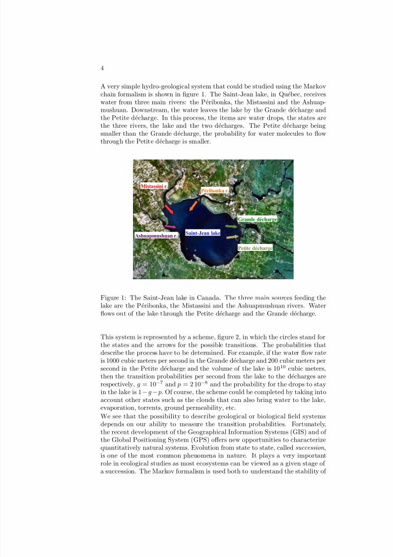
A very simple hydro-geological system that could be studied using the Markov

chain formalism is shown in figure 1. The Saint-Jean lake, in Quebec, receiveswater from three main rivers: the Peribonka, the Mistassini and the Ashuap-mushuan. Downstream, the water leaves the lake by the Grande decharge andthe Petite decharge. In this process, the items are water drops, the states arethe three rivers, the lake and the two decharges. The Petite decharge beingsmaller than the Grande decharge, the probability for water molecules to flowthrough the Petite decharge is smaller.

Péribonka r.Mistassini r.

Ashuapmushuan r.

Grande décharge

Petite décharge

Saint-Jean lake

Figure 1: The Saint-Jean lake in Canada. The three main sources feeding thelake are the Peribonka, the Mistassini and the Ashuapmushuan rivers. Waterflows out of the lake through the Petite decharge and the Grande decharge.

This system is represented by a scheme, figure 2, in which the circles stand forthe states and the arrows for the possible transitions. The probabilities thatdescribe the process have to be determined. For example, if the water flow rateis 1000 cubic meters per second in the Grande decharge and 200 cubic meters persecond in the Petite decharge and the volume of the lake is 1010 cubic meters,then the transition probabilities per second from the lake to the decharges arerespectively, g = 10−7 and p = 2 10−8 and the probability for the drops to stay

in the lake is 1−g− p. Of course, the scheme could be completed by taking intoaccount other states such as the clouds that can also bring water to the lake,evaporation, torrents, ground permeability, etc.

We see that the possibility to describe geological or biological field systemsdepends on our ability to measure the transition probabilities. Fortunately,the recent development of the Geographical Information Systems (GIS) and of the Global Positioning System (GPS) offers new opportunities to characterizequantitatively natural systems. Evolution from state to state, called succession ,is one of the most common phenomena in nature. It plays a very importantrole in ecological studies as most ecosystems can be viewed as a given stage of a succession. The Markov formalism is used both to understand the stability of

7/25/2019 Markov_GP_2015-20151202-013518683.pdf


5

an observed ecological equilibrium and to forecast the impacts of modifications

in the conditions of the equilibrium.

Pr

Mr

Ar

Sl

Gd

Pd

g

p

Figure 2: Schematic representation of the water flow through the Saint-Jeanlake. Pr, Mr and Ar represent the three upstream rivers, Sl the St-Jean lake andGd and Pd the two downstream decharges. The arrows indicate the directionof the flow. The transition probabilities from Sl to Gd and Pd are noted g and p respectively.

A fundamental property of the Markov chains is that their items are memory-

less , that is, when they are in a given state, the probabilities corresponding totheir transitions to the other states are independent of the past of the item. Inour example, the model assumes that the probabilities that a water moleculein lake Saint-Jean flows to the Petite or to the Grande decharge do not depend

on the river this water molecule came from. Moreover, in this book, we onlyconsider the so-called time homogenous Markov chains (also called stationary

Markov chains), i.e. processes in which the transition probabilities do not evolvewith time. If beavers decide to build a dam on the Petite decharge that reducesthe water flux, the corresponding Markov chain is no longer time homogenous,a new chain must be considered with a smaller transition probability betweenSaint-Jean lake and the Petite decharge. We will also only consider Markovchains with a finite number of states, which will probably not be seen as alimitation for most of our readers! It should also be underlined that the Markovformalism is, for most natural applications, only an approximate model. In ourexample, a water drop cannot immediately quit the Saint-Jean lake after havingcome out of a river, as would be the case in the Markov process. The drop hasa sort of ”memory” of when it arrived to the lake. It is therefore important for

each study using the Markovian formalism to assess the validity of the model.The Markov chains formalism allows answering a large number of questionsconcerning the process. For example: in which states the items will be foundat the end of the process? how long will they stay in each state? how manytimes will they come back to a state? will the process tend to an equilibriumsituation? if yes, which one? how will the system respond to a perturbation?etc.The objective of this book is purely pragmatic: allow students, engineers orsearchers from the different fields of natural sciences to be able to model thesystems their are interested in using the Markov formalism and to extract rele-vant information from the resulting chains in an optimum way. No mathemati-

7/25/2019 Markov_GP_2015-20151202-013518683.pdf


6

cal prior knowledge other than basic high school algebra is requested. However,

Markov chains are studied using the matrix formalism, thus for the readers notaware of the basic operations that can be applied to matrices, a three pageappendix (page ??) gives the list of the operations useful to us. Moreover, thebook is not built following the usual definition/theorem/demonstration scheme.It offers a series of tools that allow extracting information from the Markovchains and illustrate each tool by one or more examples. However, for inter-ested readers, the demonstrations of the theorems are given in appendix. All theexamples shown in this book are inspired by actual works done in a laboratoryor a company, but they are simplified for pedagogical purposes. The conclusionsdrawn from these examples are only to illustrate the kind of information thatcan be deduced from the analysis. The use of Markov chains involves algebraiccalculations, but these calculations are never made by hand. Many user-friendlycomputer softwares can be used to solve Markov algebra. The reader will find,

in appendix, small Matlab codes corresponding to all the useful calculations.The book is organized as follows. The first chapter introduces three exampleswhich are typical of three families of Markov chains: discrete absorbing processes(the time step is discrete and after a time long enough, the items are trappedinto given states), continuous processes (the items can move at any time fromone state to another, or, equivalently, the time step is infinitely small), regularprocesses (the process never stops, the items can move from state to state forever). The next chapter shows the different ways the evolution of the processcan be simulated using computer codes. Then, the different types of states andof Markov chains are detailed, as the method of analysis of chains depend ontheir type. The fourth chapter contains the algebraic methods that permit tocalculate all the relevant information about absorbing processes. It is followed

by a chapter dedicated to a series of examples of absorbing Markov chainswhere it is shown how the chain should be organized depending on the kind of information that we need to extract from it. We then turn to regular chains,that is chains with no absorbing final state. The sixth chapter is devoted to themethods of analyze for this kind of processes. The last chapter explains howto build the Markov chains, and determine the transition probabilities, for thedifferent types of systems.

7/25/2019 Markov_GP_2015-20151202-013518683.pdf


Chapter 1

Introductory examples

In this chapter, we will present three pedagogical examples corresponding tothe different kinds of Markov chains that will be studied in the book. Ourobjective is to introduce in a simple way the principal notions connected toMarkov processes and to show the kind of questions about the time evolutionof a system this formalism allows answering.

1.1 A discrete absorbing Markov process: the

under-graduated curriculum

In the first example, we characterize the evolution of a group of students in the

different levels of the bachelor curriculum. Most European countries have chosento adopt the Bologna Process which organizes a common Higher Educationframe. Following this frame, the under-graduated studies last 3 years and leadto the Bachelor degree. In the following, we will study the evolution of a cohort(i.e. a group of students entering the university the same year) along the under-graduated curriculum. The three years will be denoted B1, B2 and B3. Theyconstitute three Markov States . After three years, the students which pass thefinal exam obtain their bachelor degree, they have reached state D. Finally, eachyear, the students may fail the exams or decide to quit the curriculum, we saythat they reach state Q. The students can also redo any of the 3 years one timeor more. Each year, students have a given probability p to pass to the next level,a given probability q to quit the curriculum and a given probability r to redothe same level. To simplify a little the process, we will consider that a student

who quits the bachelor curriculum cannot come back, that the probabilities p,q and r are the same along the three years and that a student can redo thesame level with no limit. The corresponding Markov chain is shown in figure1.1. As can be seen, the Markov chain is composed of states and of transitionsfrom state to state, each transition being characterized by a probability. It canalso be seen that the chain is not necessarily a linear set of transitions, it cancontain forks and even cycles. Each year each student moves from one state toanother or stays in the same state. When a student reaches states D or Q, theprobability that he/she stays in this state the next year is 1. At the end of eachyear, the only possibilities for a student is to pass to the next level, redo thelevel or to quit the curriculum, thus p + q + r = 1. We could have represented on

7

7/25/2019 Markov_GP_2015-20151202-013518683.pdf


8 CHAPTER 1. INTRODUCTORY EXAMPLES

the scheme the latency loops , that is the arrows connecting each state to itself

with probability r for the B states and 1 for the D and Q states but, as this isnot useful, this is usually not done.

B1 B2 B3

Q

D

p p p

q q q

Figure 1.1: The 5 states and 6 transition probabilities for the under-graduatedcurriculum Markov chain. In this figure and the following, the small red arrowindicates the entrance in the chain.

Let’s now consider that a student entering the curriculum. The questions he/sheis interested in are typically to know what is the probability to obtain thedegree and how long it will take on average. These questions are not easyto answer since the diploma can be obtained following different ”paths”, byredoing, possibly several times, some levels. For example, if the probabilities

are the following: p = 0.7, q = 0.2 and r = 0.1, most people would think that,by rule of thumb, the probability to obtain the bachelor degree is larger thanthe probability to quit. In fact, as we will see, the degree probability is only47%. The Markov formalism allows answering the above questions, and manyothers, in a very elegant and simple way.The Markov chain is formalized by states and transition probabilities . Thechain by itself does not change year after year. What evolves is the numberof students in each level. This is described by the so-called population vector

n. In our case, the population vector is n =

B1

B2

B3

DQ

where Bi is the number

of students in level i, D the number of students that have obtained the degreeand Q the number of students that have quit the curriculum. The sum of the

components of the population vector is, of course, a constant. This is why,in many cases, the components of the vector are divided by the sum of thecomponents, so that the population vector contains proportions. In this case,the components can be seen both, as the proportion of students in each stateor as the probability for a given student to be in each of the states. This is thereason why the normalized population vector is often called the state probability

vector , the sum of its components is one.Suppose that the distribution of the students at year y is given by n and thedistribution of the students at year y + 1 is given by n, how can we writethe components of n as a function of the components of n ? Lets, for example,consider the students in state B2 at year y +1. The previous year, these students

7/25/2019 Markov_GP_2015-20151202-013518683.pdf


1.1. A DISCRETE ABSORBING MARKOV PROCESS: THE UNDER-GRADUATED CURRICULUM 9

where either in state B1 and they passed to B2 with probability p or in state B2

and they redo the same level with probability r. Thus, B

2 = p B1+(1− p−q ) B2.Using the same line of thought, we can write the following equations:

B1 = (1 − p − q ) B1

B2 = p B1+ (1 − p − q ) B2

B3 = p B2+ (1 − p − q ) B3

D = p B3+ DQ = q B1+ q B2+ q B3+ Q

(1.1)The first line says that the only way to be in level B 1 at year y + 1 is to alreadybe in B1 the previous year as we consider only one cohort of students. The lasttwo lines show that the number of students in state D and Q can only increase

year after year since the students already present in these states at year y willstill be there at year y + 1. The terms in equations (1.1) corresponding to thesame level are aligned in order to show that this system of linear equations canalso be written using the matrix formalism as:

n = M n , (1.2)

Where

M =

1 − p − q 0 0 0 0 p 1 − p − q 0 0 00 p 1 − p − q 0 00 0 p 1 0

q q q 0 1

(1.3)

is the transition matrix also called Markov matrix. It is worth noticing that,whereas vector n evolves year after year, matrix M does not change.Here, in order to build the transition matrix, we have first written the systemof linear equations (1.1). In fact, we usually do not proceed in this way. Indeed,as can be seen, matrix M is composed of probabilities. To understand howthese probabilities are arranged, we rewrite the matrix indicating the statescorresponding to each row and column:

B1 B2 B3 D Q

M =

1 − p − q 0 0 0 0

p 1 − p − q 0 0 00 p 1 − p − q 0 00 0 p 1 0q q q 0 1

B1

B2B3

DQ

(1.4)

´ ´ ´ ´ ´

= 1 = 1 = 1 = 1 = 1

Each row contains the probabilities to go to a given state from the differentstates. For example, the last row contains the probabilities to go to the Q state.It is composed of three q which are the probabilities to go from one level of thecurriculum to the Q state, a 0 which is the probability to go from D to Q and a 1

7/25/2019 Markov_GP_2015-20151202-013518683.pdf



which is the probability to stay in the Q state when already in it. The columns

contain the probabilities to quit or to stay in a given state. For example, the firstcolumn, relative to B1 is composed, from top to bottom, by 1− p−q which is theprobability to stay in B1, p the probability to go to B2, zeros and q which is theprobability to quit the curriculum. As can be seen, the sum of the probabilitiesto leave or to stay in a given state is always 1 (this is a good way to verifythat your Markov matrices do not contain errors). To build the matrix directlyfrom the scheme given in figure 1.1, one just has to fill it by the probabilitiesto go from the column states to the row states. For example, the red p is theprobability to go from the B2 state to the B3 state. If there is no arrow in thescheme then the probability is 0. The probabilities we are talking about areso-called conditional probabilities. They are not simply the probabilities of astate A but the probabilities of being in a state A given that we were in stateB the previous year. Conditional probabilities are written in the following way:

P (A|B) which reads ”probability of A given B”. Moreover, the components of a matrix X are, by convention, noted X ij where the first index, i, is the numberof the row and and the second, j, is the number of the column. Hence, thecomponents of the transition matrix will be noted M i|j in this book. Using thisnotation, we see, for example, that p is M B3|B2

. Be careful that the order of theindexes may seem counterintuitive: the new state is placed first and the initialstate is placed second. The components out of the diagonal are the probabilitiesto change state. They are obtained by considering the arrows in figure 1.1. Thecomponents on the diagonal are the probabilities to remain in the same state.They are obtained as 1 minus the sum of the other probabilities in the samecolumn. Hence, it is not necessary to write the system of linear equations: inpractical applications, the transition matrix is built directly from the scheme of

the Markov process (figure 1.1). The scheme also helps us calculate easily theprobability P of given tracks , that is successions of states (i0, i1, . . . in). Thetrack probability depends on the probability to be initially in states i0, that isni0(0), and on the different transition probabilities from state to state:

P (i0, i1, . . . in) = ni0(0) M i1|i0 M i2|i1 . . . M in|in−1 (1.5)

For example, the probability for a student to begin in B1, then pass to B2, thenredo B2, then pass to B3, then quit the curriculum is P = 1 p r p q = 0.0098.This first chain corresponds to a so-called discrete Markov process as the pop-ulation of students can move from one state to another only after a given timelapse called the time step (here ∆t = 1 year). We now turn to continuousprocesses.

1.2 A continuous absorbing Markov process:

the radioactive double decay

In environmental studies, most Markov processes do not respect regular discretetime steps. For example, pollutant molecules emitted by an industrial plant toa river can be absorbed at any time by a fish (in this case, the river and the fishare states and the population is made of pollutant molecules). Nevertheless,such continuous processes can also be studied using the Markov formalism.To illustrate this, we consider the case of a radioactive double decay. Radium

7/25/2019 Markov_GP_2015-20151202-013518683.pdf


1.2. A CONTINUOUS ABSORBING MARKOV PROCESS: THE RADIOACTIVE DOUBLE DECAY 11

(226Ra) is a radioactive element which is present in many rocks, notably granite.

It is an alpha emitter, which means that it can emit an alpha particle made of 2 neutrons and 2 protons. It is then transformed into radon ( 222Rn), which is agas, and may leave the rock and enter the atmosphere. Radon is also radioactive.It is the main source of natural ground radioactivity for humans as we can inhaleit. Radon is also an alpha emitter, it decays to polonium (218Po). The decaywill continue after polonium through a sequence of radioactive nuclei down tolead 206Pb, which is stable. However, here we will consider only three states of the nuclei: Ra, Rn and Pof (which contains polonium and its followers).

!1

Ra Rn Pof!2

Figure 1.2: The radioactive double decay.

A radium nucleus decays into radon after, on average, 2309 years, whereas aradon nucleus decays into polonium after only 5.5 days on average. This meansthat during a given time lapse, say one year, the decay probability of a radiumnucleus is low (high average time) whereas the decay probability of a radonnucleus is high (low average time). Therefore, we characterize the transition bythe inverses of the average decay times: the transition Ra → Rn has a rate-

constant 1 λ1 = 1/2309 year−1 and the transition Rn → Pof has a rate-constantλ2 = 1/5.5 day−1. Be careful that rate-constants are not times but inverses of time, that is frequencies. Let’s consider a time-lapse dt. We have the followingproperty:”If dt is very small compared to 1/λ then λ dt is the transition probabilityduring time dt”.For example, if we take dt = 1 year, the probability that a given radium nu-cleus decays is actually 1/2309. This would not be valid for the radon decay:indeed, in this case, λ2 dt = 1/5.5 day−1 × 1 year = 66 which is obviously nota probability. In fact, the probability that a given radon nucleus decays withinone year is very close to 1, since 1/λ2 is very small compared to one year. Inorder to express the transition probability from Rn to Pof, we have to considera time step small with respect to 5.5 days, for example one hour, in which case,the probability reads P = 1/5.5 day−1 × 1 hour = 0.0076. Finally, we can seethat the double radioactive decay can be represented by a Markov chain, as we

have states (Ra, Rn, Pof), a population made of nuclei evolving from state tostate and probabilities to go from one state to another: λ1 dt and λ2 dt (seefigure 1.2, note that, in the case of a continuous process, the rate-constants arewritten on the arrows of the scheme instead of the probabilities). The formalismused to study continuous processes is the same as for discrete processes but thetime step dt has to be very short with respect to all the times that play a rolein the process. Here dt has to be small with respect to both 1/λ1 = 2309 yearsand 1/λ2 = 5.5 days. For computer codes used to calculate Markov processes,

1Rate constants, also called ”radioactive constants” in the case of radioactivity, are relatedto the so-called ”half-life” T 1

2

of the element by the following formula: λ = ln(2)/T 12

. The

half-life is the time after which one half of a set of radioactive nuclei has decayed.

7/25/2019 Markov_GP_2015-20151202-013518683.pdf



the time step value has to be of the order of one-hundredth of the minimum

inverse rate-constant to obtain reliable results, here, dt = 5.5/100 day, we willcome back to this question in the next chapter. The Markov matrix of the dou-ble decay can be built by considering the probabilities to go from one state toanother during a small time step. One obtains:

Ra Rn Pof

M =

1 − λ1 dt 0 0

λ1 dt 1 − λ2 dt 00 λ2 dt 1

Ra

RnPof

(1.6)

The way this matrix can also be built using the differential equations thatdescribe the double decay is explained in the Demonstration appendix page ??.This transition matrix is used exactly in the same way as the transition matrices

for discrete processes except that the time lapse is now dt. Therefore, the timeevolution of the population is given by:

n(t + dt) = M n(t) . (1.7)

Where n =

RaRn

P of

is the population vector. It contains the numbers of radium,

radon and polonium+follower nuclei. For example, the second line of equation(1.7) is Rn(t + dt) = Rn(t) + λ1 dt Ra − λ2 dt Rn, which means that, duringtime dt the number of radon nuclei has increased by λ1 dt Ra and decreased by−λ2 dt Rn. More generally, we call the sum of the positive terms proportionalto dt in such equations, the production rate of the state and the sum of thenegative terms, the decay rate . If the production and decay rates are the same,

then the population of the state stays constant.

1.3 A regular Markov process: forest succession

In both preceding examples, after a time long enough, all the items of thepopulation are located in the so-called absorbing states: Q and D in the first caseand Pof in the second. Another kind of processes, called regular Markov chains,contains no absorbing states. The items will move from one state to anotherfor a theoretically infinite time. For example, water molecules can evaporatefrom the ocean to clouds, fall on the ground, reach a river back to the oceanand then evaporate again. This is a very simple circular regular chain includingfour states: Oceans, Clouds, Ground and Rivers. There is no absorbing states,

only four transient states. What could interest us in this example could be theaverage quantities of water in the different states, or, said in another way, howlong on average water molecules remain in each state.The evolution of the coverage of landscapes is often studied using the Markovchain formalism. We consider a simplified example of forest succession. In agiven region, the forests are made of three types of trees: Aspen, Pine and Limetree. Each kind of tree comes into two stands Young and Mature. Thus, sixstates noted as: Ay, Am, Py, Pm, Ly and Lm can be defined. The scheme ispresented in figure 1.3When mature trees die, they are replaced by a young tree of the same species orof another species. The six components of the population vector represent the

7/25/2019 Markov_GP_2015-20151202-013518683.pdf


1.3. A REGULAR MARKOV PROCESS: FOREST SUCCESSION 13

Py Pm

Ay Am

Ly Lm

g A

g P

g L

r A

pP|A pL|A

pA|P

r P pL|P

pA|L pP|L

r L

Figure 1.3: Natural forest succession including three tree species (blue: aspen,

purple: pine, green: lime tree) and to maturity stages (light color: young, darkcolor: mature).

surface covered by each kind of trees (young or mature). We choose the timestep to be five years. The transition matrix reads:

Ay Am Py Pm Ly Lm

M=

1−gA rA 0 pA|P 0 pA|L

gA 1−rA− pP|A− pL|A 0 0 0 0

0 pP|A 1−gP rP 0 pP|L

0 0 gP 1−rP− pA|P− pL|P 0 0

0 pL|A 0 pL|P 1−gL rL

0 0 0 0 gL 1−rL− pA|L− pP|L

Ay

Am

Py

Pm

Ly

Lm

(1.8)

As will be seen in the following chapters, this matrix allows calculating theevolution of the forest coverage and study the kind of long-time equilibriumwhich can be spontaneously reached. The transition probabilities are deducedfrom the observation of actual forests. It is also possible, using the formalism,to study the influence of human interference. We could imagine, for example,that forest managers continuously replace half of the dead aspens and lime treesby pines. This can be simulated by modifying the transition probabilities in thetransition matrix. Hence, the Markov formalism may be of great help to assesthe long-term consequences of perturbation on natural systems.

7/25/2019 Markov_GP_2015-20151202-013518683.pdf



7/25/2019 Markov_GP_2015-20151202-013518683.pdf


Chapter 2

Time evolution of a Markov

process

2.1 Evolution using transition matrix powers

We have seen that, for a Markov process, the population vector at time t + ∆tcan be calculated from the population vector at time t using the transitionmatrix: n(t + ∆t) = M n(t) where ∆t has to be very small in the case of a continuous process. If we apply the formula at time 0, we obtain n(∆t) =M n(0). Similarly, n(2 ∆t) = M n(∆t), which can be rewritten, using the

previous equation, n(2 ∆t) = M2 n(0). Thus, the population vector at time tis:

n(t) = Mn n(0) with t = n ∆t . (2.1)

This is a very important feature of Markov processes: the populations at anytime can be calculated from the initial population vector and the transitionmatrix only. Moreover, in the same way as the components of the M matrixare the probabilities to go from state j at time t to state i at time t + ∆t,the Mn matrix is composed of the probabilities to go from state j at time t tostate i at time t + n ∆t. The Matlab code used to calculate the time evolution,

using transition matrix powers, for the bachelor curriculum example is given inSection ??.

2.2 Results for the introductory examples

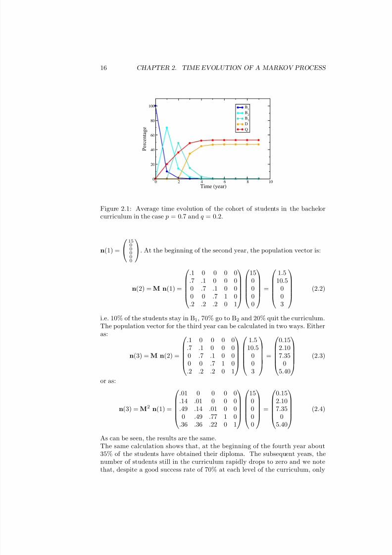
In the case of the bachelor degree, figure 1.1, the average time evolution curvesare given in figure 2.1.

Initially all the students are in level B1, thus the initial population vector is

15

7/25/2019 Markov_GP_2015-20151202-013518683.pdf


16 CHAPTER 2. TIME EVOLUTION OF A MARKOV PROCESS

0 2 4 6 8 10

Time (year)

0

20

40

60

80

100

P e r c e n t a g e

B1

B2

B3

D

Q

Figure 2.1: Average time evolution of the cohort of students in the bachelorcurriculum in the case p = 0.7 and q = 0.2.

n(1) =

15

00000

. At the beginning of the second year, the population vector is:

n(2) = M n(1) =

.1 0 0 0 0

.7 .1 0 0 0

0 .7 .1 0 00 0 .7 1 0.2 .2 .2 0 1

150

000

=

1.510.5

003

(2.2)

i.e. 10% of the students stay in B1, 70% go to B2 and 20% quit the curriculum.The population vector for the third year can be calculated in two ways. Eitheras:

n(3) = M n(2) =

.1 0 0 0 0

.7 .1 0 0 00 .7 .1 0 00 0 .7 1 0.2 .2 .2 0 1

1.510.5

003

=

0.152.107.35

05.40

(2.3)

or as:

n(3) = M2 n(1) =

.01 0 0 0 0

.14 .01 0 0 0

.49 .14 .01 0 00 .49 .77 1 0

.36 .36 .22 0 1

150000

=

0.152.107.35

05.40

(2.4)

As can be seen, the results are the same.The same calculation shows that, at the beginning of the fourth year about35% of the students have obtained their diploma. The subsequent years, thenumber of students still in the curriculum rapidly drops to zero and we notethat, despite a good success rate of 70% at each level of the curriculum, only

7/25/2019 Markov_GP_2015-20151202-013518683.pdf


2.2. RESULTS FOR THE INTRODUCTORY EXAMPLES 17

47% of the cohort obtain their bachelor degree. The population vector may

contain the number of students in each state. It can also be normalized , thatis divided by the total number of students, in which case the components arethe probability for a student to be in each state. If the normalized vector ismultiplied by 100, then it contains the percentage of students in each state. Inall cases, the n vector is handled in the same way and equation (2.1) holds. Itis important to realize that these curves can be read both as the proportion of students in each level or as the probability for a given average student to be inthe different states, year after year.

1e-03 1e-02 1e-01 1e+00 1e+01 1e+02 1e+03 1e+04 1e+05

Time (year)

1e-08

1e-07

1e-06

1e-05

1e-04

1e-03

1e-02

1e-01

1e+00

P r o p o r t i o n

RaRnPof

Figure 2.2: Time evolution of the proportion of radium (black), radon (red) andpolonium+followers (blue) nuclei.

The time evolution of the population vector in the case of the double decay,figure 1.2, is calculated in the same way. The time step has to be very shortand the curves are ”smooth”. In our decay, the rate-constant λ2 is much largerthan λ1. The arrows between the states can be visualized as pipe, the sectionof which being the rate-constant or the probability (see for example figure 2.4).Hence, the Ra nuclei turn very slowly into Rn nuclei and then rapidly into Ponuclei. This means that the number of Rn nuclei will always be very smallcompared to Rn nuclei or Po + followers nuclei. This is the reason why thefigure 2.2 had to be plotted with logarithmic axes.

In the case of the forest succession process, figure 1.3, the population vectoris calculated every five years. We have chosen two different initial allocationsof the forest surface. The results are shown in the top of figure 2.3. In thefirst one, left plot, the initial surface is covered by young trees only. In thesecond one, right plot, the surface is the same for each state. In both cases, thevariations of the populations are initially fast and complex. After thirty yearsthe evolution slows down. The remarkable result is that, after about eightyyears, the distribution of the surface amongst the six states is the same for bothinitial distributions. In the right figure, a disease is simulated at year 100, thatkills all the young and mature aspens. Their percentages fall to zeros and, as aresult, the other percentages are increased. Once more, after a recovery time,

7/25/2019 Markov_GP_2015-20151202-013518683.pdf



the same repartition of the surface is reached. This behavior is not intuitive,

here the Markov formalism may give us a hint on why nature is able to recoverits prior appearance even after important external perturbations. The mathe-matical reasons underlying such a behavior and the method to predict the finaldistribution will be addressed in Chapter 4.

0 50 100 150 200 250 300

Time (year)

20

40

60

80

100

P e r c e n t a g e

o f t h e

s u r f a c e

Ay

AmPy

PmLy

Lm

a)

0 50 100 150 200 250 300 350 400

Time (year)

20

40

60

80

100

P e r c e n t a g e

o f t h e

s u r f a c e

Ay

AmPy

PmLy

Lm

b)

0 50 100 150 200 250 300

Time (year)

20

40

60

80

100

P e r c e n t a g e

o f t h e

s u r f a c e

Ay

AmPy

PmLyLm

c)

Figure 2.3: Time evolution of the surface covered by different kinds of trees inthe case of a natural succession. a) initially the surface is shared between theyoung tree states only. b) initially the forest surface corresponding to the sixstates is the same. At year 100, a disease kills all the aspens in the forest. Itis remarkable that, in every case, the evolution tends towards the same statedistribution, see the proportions inside the red ovals. c) the forest is maintainby man, one half of the dead aspens and lime trees are replaced by pines.

We now turn to the case when the evolution is perturbed by man: one half of the dead aspens and lime trees are replaced by pines. Of course, the finalsurface repartition is affected, see figure 2.3 bottom plot. However, the aspensand lime trees do not disappear, after about 50 years, their proportions stabilizeagain but at a much lower value. The relative proportions of young and adulttrees are the same as for the natural evolution.

2.3 Iterative calculation of the time evolution

We have seen that, for continuous processes, the time step dt has to be aboutone hundredth of the smallest inverse rate-constant. Moreover, in order to reach

7/25/2019 Markov_GP_2015-20151202-013518683.pdf


2.3. ITERATIVE CALCULATION OF THE TIME EVOLUTION 19

the saturation, the evolution has to be calculated up to a time 10 to 100 larger

than the largest inverse rate-constant. In the double decay case, the two rate-constants have very different orders of magnitude since λ2 is about 150 thousandtimes larger than λ1. Thus, the time step has to be extremely small comparedto the total time. This entails that, to calculate the whole evolution, it wasnecessary to multiply the transition matrix about 10 million times by itself.Since our three state process is very simple and our transition matrix has onlythree rows and three columns, it has been possible to compute the evolutionwithin a short computer time. However, for more complex systems, with muchmore states and even larger differences between the orders of magnitude of therate-constants, which is a usual case in natural studies, the calculation would beimpossible even using the most powerful computers. To illustrate what happensfor bad choices of the time step duration or of the number of time steps, weconsider the basic example of figure 2.4 in which the transitions from state 1 to

state 2 and state 3 are fast and the transition from state 2 to state 3 is veryslow.

A C

B

! 3

! 2

! 1

Figure 2.4: Markov process. The initial state is A and the final one is C.The rate-constants λ1 and λ2 are, respectively, 10 and 20. The rate-constantλ

3 = 0.001 is much smaller.

2.3.1 Right choice for the time step

In our example, dt has to be small with respect to the minimum inverse rate-constants that is to 1/λ1 = 0.1. Figure 2.6 shows what happens, at the beginningof the evolution, for different choices of the time step duration.In this case, we see that for time steps lower than 0.2, that is 1 /50× 1/λ2, thecalculated evolutions are the same. On the other hand, for time steps longerthan 2, differences are visible. This kind of analysis allows setting the value of the time step for any Markov process simulation. In the large majority of the

cases, one hundredth of the minimum inverse rate-constant is a safe choice.

2.3.2 Right choice for the number of time steps

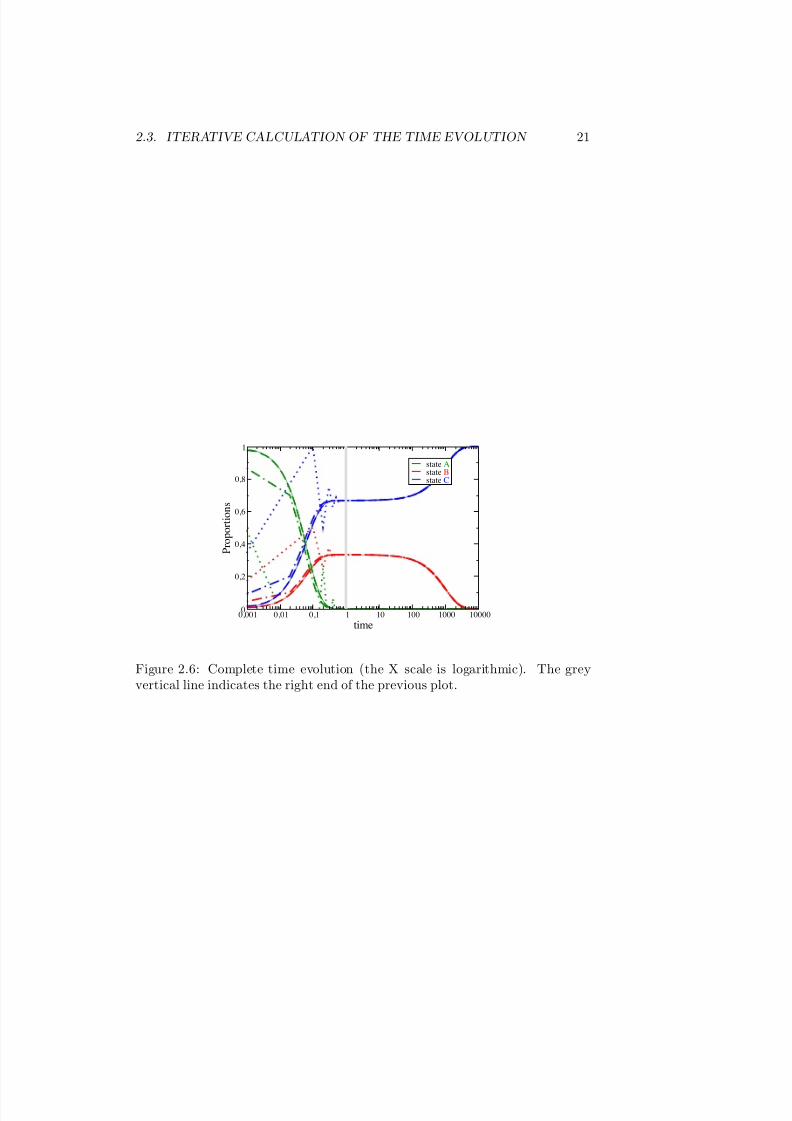
The total time of the calculated evolution must be large with respect to thevalue of the maximum inverse rate-constant. Visually, at the end of the process,the proportions in the different states should not evolve any longer. This is thecase, for example, in figure 2.3. Nevertheless, the stabilization of the curves isnot by itself a proof that the saturation is reached. Indeed, in figure 2.6, theproportions seem stable and the final equilibrium reached. However, this is notthe case: at time t = 1, one third of the population is in state B which has a

7/25/2019 Markov_GP_2015-20151202-013518683.pdf



0 0,2 0,4 0,6 0,8 1

time

-0,4

-0,2

0

0,2

0,4

0,6

0,8

1

P r o p o r t i o n s

state Astate Bstate C

Figure 2.5: Time evolution of the population vector for the scheme shown in theprevious figure. Initially, the probability to be in state A is 1. The line stylesindicate the values of the time steps used in the calculation: dt = 0.01 (thinlines), 0.2 (dashed lines), 2 (dot-dashed lines), 10 (dotted lines). The thin linesand the dashed lines are superposed, thus, for simulation time steps d t lowerthan 0.2, the results are the same.

very slow rate constant to state C. Therefore, B stands as a reservoir with avery small leak towards C. This is not visible in figure 2.6, but the proportion

in B is decreasing very slowly. The rate-constant from B to C is 0.001, thus theevolution time should be much larger than 1000. The right result is shown infigure 2.6 with a log scale horizontal axis. We see a plateau between time 0.5and 50 followed by a decrease of the B proportion reaching zero around time5000. We also note that the problems due to the choice of a too large time stepare mostly seen at the beginning of the evolution.Other arguments to determine the number of steps, depend on the type of thechains. They will be introduced latter on:

• For absorbing chains, another way to check that the evolution has ended isto calculate the so-called absorption matrix that gives the final proportionsin each state, as will be shown in section 3.2.5.

• For regular chains, the final proportions are given by the stationary dis-tribution, equation (4.3), and the minimum number of time steps can becalculated a priori: it has to be at least of the order of the convergence

time T 110

, equation (4.8).

7/25/2019 Markov_GP_2015-20151202-013518683.pdf


2.3. ITERATIVE CALCULATION OF THE TIME EVOLUTION 21

0,001 0,01 0,1 1 10 100 1000 10000

time

0

0,2

0,4

0,6

0,8

1

P r o p o r t i o n s

state Astate Bstate C

Figure 2.6: Complete time evolution (the X scale is logarithmic). The greyvertical line indicates the right end of the previous plot.

7/25/2019 Markov_GP_2015-20151202-013518683.pdf



7/25/2019 Markov_GP_2015-20151202-013518683.pdf


Chapter 3

Absorbing Markov chains

In this chapter, we will consider the absorbing Markov processes , that is pro-cesses in which all final states are absorbing. This means that after a time longenough, each item of the population is stable in its final state. Before enteringthis chapter, it is recommended to read the first two introductory examples,sections 1.1 and 1.2. In the following, we will see that most of the relevantinformation concerning a Markov process can be deduce directly from the tran-sition matrix. For example, the students in the different levels can calculatetheir probabilities to obtain their degree, or the average times they will spendon the next levels. Therefore, one does not necessarily need to build the timeevolution of the population vector as seen in the previous chapter. In somecomplex continuous cases, this is not even possible due to computer limitations.

Moreover, some information like the probability for a student to remain a givennumber of years in a given level, or the dispersion of the times spent by thestudents in a given level, cannot be deduced from the average time evolution.Besides, using matrix algebra in stead of numerical calculation of the time evo-lutions, one obtains the algebraic expressions of the relevant quantities whichmay allow a better understanding of the process, or, as we will see, may allowto optimize the parameters (transition probabilities) of a Markov chain. Thepresent chapter shows how this information can be extracted from the transitionmatrix only, using the simple matrix algebra recalled in Appendix A.

3.1 The transition matrix M

3.1.1 Canonical form

The transition matrix of a given Markov process is not unique since we canchoose arbitrarily the order of the states. However, the order must be the samefor the rows and the columns of the transition matrix and for the populationvector. To facilitate the handling of the matrix, we now impose to write it underits so-called canonical form . This simply means that final states are placed firstin the state order. Thus, we still have arbitrary choices to make since the orderof the final states, as well are the order of the transient states, are not fixed.For example, in the case of the bachelor curriculum, the transition matrix canbe rewritten under the following canonical form:

23

7/25/2019 Markov_GP_2015-20151202-013518683.pdf


24 CHAPTER 3. ABSORBING MARKOV CHAINS

D Q B1 B2 B3

M =

1 0 0 0 p0 1 q q q 0 0 1 − p − q 0 00 0 p 1− p− q 00 0 0 p 1− p− q

DQB1

B2

B3

(3.1)

Of course, the sum of the components of every column is still 1. As can be seen,we like to separate the transition matrix into four quadrants corresponding toabsorbing and transient states. These quadrants are also matrices, they aregiven names as follows:

M =

I R0 Q

(3.2)

The upper left quadrant contains the transition probabilities from final statesto final states. As these states are absorbing, the probabilities to leave them are0 (components out of the diagonal of the quadrant) and the probabilities stayin them are 1 (on the diagonal). Hence, the I matrix is the identity matrix andits numbers of rows and columns are the number of final states. The lower leftmatrix corresponds to the transitions between a final state and a transient state,thus all the components are zeros. The 0 matrix is a zero matrix which numberof rows is the number of transient states and number of column is the number of final states1. The R matrix contains the transition probabilities from transientstates to final states and the Q matrix contains the transition probabilities from

transient states to transient states. Both latter matrices depend on the Markovprocess under study and on the chosen order of the states.Another advantage of writing the transition matrix under the canonical formis that the calculation of its powers is made easier. The square of the matrix

reads M2 =

I R (I+Q)

0 Q2

and, more generally:

Mn =

I R (I + Q + . . . + Qn−1)0 Qn

, (3.3)

thus the I and the 0 quadrants do not change when the matrix is multiplied byitself.

3.1.2 The M∞

matrixDefinition

The final distribution of the items of the population among the final statescan be calculated from the initial distribution by writing n(t) = Mn n(0) witht = n ∆t very large (n and t = n ∆t ”tend to infinity”). In fact, dependingon the processes under study, a ”very long time” may be reached after only asmall number of time steps as it is the case for our bachelor curriculum examplewhere the final proportions are almost attained after only 5 iterations (see figure

1In the following all identity matrices and all zero matrices will be noted respectively I and0 whatever their dimensions.

7/25/2019 Markov_GP_2015-20151202-013518683.pdf


3.1. THE TRANSITION MATRIX M 25

2.1). On the other hand, for complex continuous processes mixing very small

and very large rate-constants, the convergence may be reached after extremelylarge numbers of steps. By misnomer, we will write (from equation (3.3)):

M∞ =

I R (I + Q + . . . + Q∞)0 Q∞

and (3.4)

n(∞) = M∞ n(0) (3.5)

We now introduce two new matrices: F = I + Q + . . . + Q∞ the fundamental

matrix and A = R F the absorption matrix so that:

fin. tr.

M∞ = I A

0 Q∞ final

transient (3.6)

This matrix can be read in the same way as the M matrix: its componentsM ∞

i|j are the probabilities to go from the jth state at time 0 to the ith state attime ∞. The sum of the probabilities in each column has also to be 1. Aftera very long time, all the population has left the transient states, e.g. no morestudents are present in the bachelor curriculum levels. Hence, the probabilitiesto go from a transient state to a transient state are all equal to zero. This showsthat Q∞, is a zero matrix, thus:

M∞ =

I A

0 0

(3.7)

The only non-trivial part of this matrix is the upper right one. It contains theprobabilities to go from the different initial states to the different final states,for example, the probability for a freshman to finally pass the degree.

Use in time evolution codes

We now turn to the final population vector. After a time long enough, allthe items of the population are located in the absorbing states. Therefore,the population vector will not evolve any longer. Said in a mathematical way:M n(∞) = n(∞) and, more generally, Mn n(∞) = n(∞). Using equation(3.5), this gives n(∞) = M∞ Mn n(0), thus, for any time t:

M∞ n(t) = n(∞) (3.8)

This equation may seem surprising: the left hand side appears as depending ontime whereas the right hand side is a constant. In fact, this is a characteristicof the M∞ matrix, it projects the population vector onto the space of the finalstates where it is constant. This property can be used in the iterative codesthat calculate the time evolution of the system, in the case of very long timeevolution, to check that the calculation is stable, that is, is not affected bythe successive rounding errors: the value of M∞ n(t) is regularly compared toM∞ n(0) to check that it does not diverge.

7/25/2019 Markov_GP_2015-20151202-013518683.pdf



3.2 Characteristics of the process obtained us-

ing matrices

3.2.1 The fundamental matrix F

In the previous section, we have introduced the fundamental matrix F. As weare going to see, this matrix holds interesting information about the durationsof the stays of the population in the different states. It is evident that thecalculation of the fundamental matrix from the infinite sum of the successivepowers of Q would be intractable. Fortunately, it can be calculated in a muchmore convenient way as:

F = (I − Q)−1 , (3.9)

The way to compute, using the Matlab language, the fundamental matrix, aswell as all the matrices introduced in the present chapter, is shown page ??. Ascan be seen, most equations correspond to as single Matlab line.

The component F i|j of the fundamental matrix is the number of time steps anitem of the population will spend in the transient state i after being in thetransient state j. The demonstration is given page ??. For example F B3|B2

isthe average number of time steps (years) a student in level B 2 will spend inlevel B3. This number is not the same as F B3|B1

since some freshmen will nevergo to B3 because they quit the curriculum: these students will spend 0 years inB3 so they contribute to decrease the average number of years a freshman willspend in B3 with respect to a sophomore.

3.2.2 The time matrix T

As we are interested in the time spent in the states rather than by the numberof time steps, we introduce the time matrix

T = ∆t F , (3.10)

which components T i|j are the average times spent in the transient states i afterbeing in the transient states j.

Examples

We first consider the case of the double radioactive decay. The transient statesare Ra and Rn. The Q matrix, which contains the transition probabilitiesbetween transient states, reads:

Ra Rn

Q =

1− λ1 dt 0

λ1 dt 1− λ2 dt

Ra

Rn (3.11)

so that I−Q =

λ1 0−λ1 λ2

dt. Its inverse is F =

1

λ10

1

λ2

1

λ2

1dt

(inverse of matrices

7/25/2019 Markov_GP_2015-20151202-013518683.pdf


3.2. CHARACTERISTICS OF THE PROCESS OBTAINED USING MATRICES 27

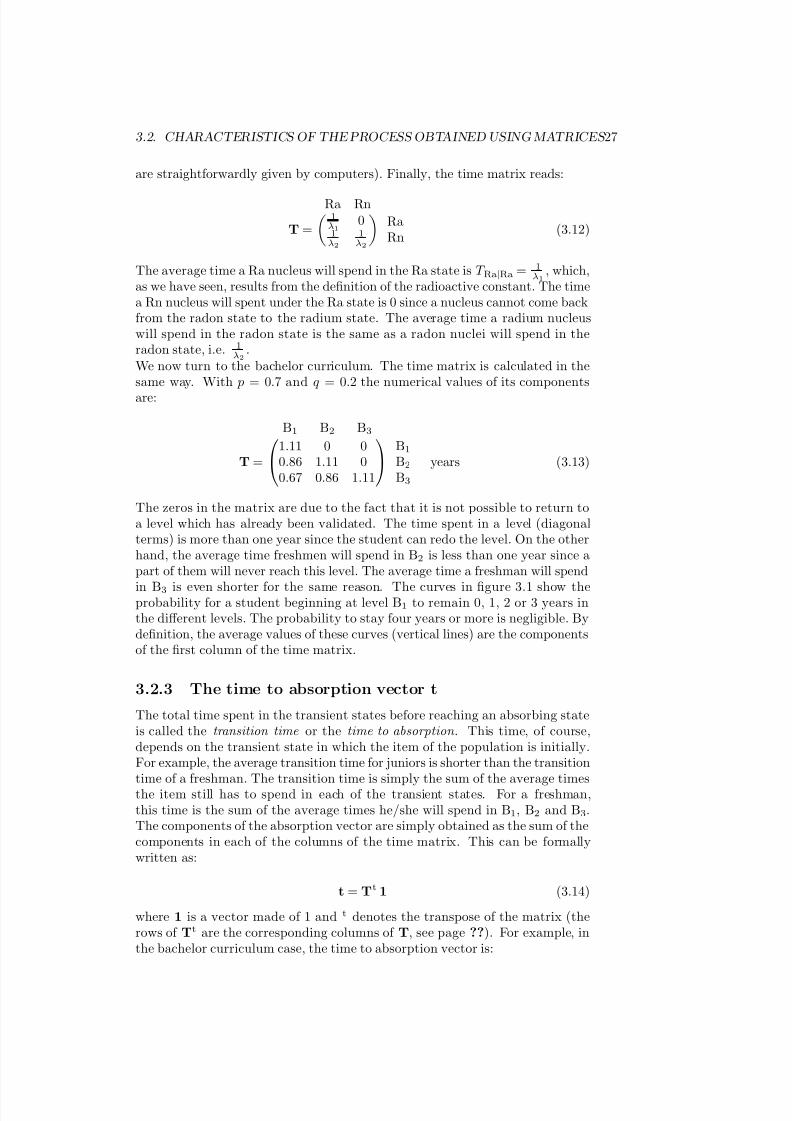
are straightforwardly given by computers). Finally, the time matrix reads:

Ra Rn

T =

1λ1

01

λ2

1λ2

Ra

Rn (3.12)

The average time a Ra nucleus will spend in the Ra state is T Ra|Ra = 1λ1

, which,as we have seen, results from the definition of the radioactive constant. The timea Rn nucleus will spent under the Ra state is 0 since a nucleus cannot come backfrom the radon state to the radium state. The average time a radium nucleuswill spend in the radon state is the same as a radon nuclei will spend in theradon state, i.e. 1

λ2.

We now turn to the bachelor curriculum. The time matrix is calculated in thesame way. With p = 0.7 and q = 0.2 the numerical values of its components

are:

B1 B2 B3

T =

1.11 0 0

0.86 1.11 00.67 0.86 1.11

B1

B2

B3

years (3.13)

The zeros in the matrix are due to the fact that it is not possible to return toa level which has already been validated. The time spent in a level (diagonalterms) is more than one year since the student can redo the level. On the otherhand, the average time freshmen will spend in B2 is less than one year since apart of them will never reach this level. The average time a freshman will spend

in B3 is even shorter for the same reason. The curves in figure 3.1 show theprobability for a student beginning at level B1 to remain 0, 1, 2 or 3 years inthe different levels. The probability to stay four years or more is negligible. Bydefinition, the average values of these curves (vertical lines) are the componentsof the first column of the time matrix.

3.2.3 The time to absorption vector t

The total time spent in the transient states before reaching an absorbing stateis called the transition time or the time to absorption . This time, of course,depends on the transient state in which the item of the population is initially.For example, the average transition time for juniors is shorter than the transition

time of a freshman. The transition time is simply the sum of the average timesthe item still has to spend in each of the transient states. For a freshman,this time is the sum of the average times he/she will spend in B1, B2 and B3.The components of the absorption vector are simply obtained as the sum of thecomponents in each of the columns of the time matrix. This can be formallywritten as:

t = Tt 1 (3.14)

where 1 is a vector made of 1 and t denotes the transpose of the matrix (therows of Tt are the corresponding columns of T, see page ??). For example, inthe bachelor curriculum case, the time to absorption vector is:

7/25/2019 Markov_GP_2015-20151202-013518683.pdf



0 1 2 3Time (year)

0

0.2

0.4

0.6

0.8

1

P r o b a b i l i t y

TB

2|B

1

TB

1|B

1

TB

3|B

1

B1

B2

B3

!"#

!"#

#

!"#$

"##

!"#

#"#

#

Figure 3.1: Distributions of the probabilities for the students to stay between 0and 3 years in the different levels. The averages values of the distributions areindicated by vertical lines and the standard deviations by arrows.

t = 2.651.981.11

B1

B2B3

years (3.15)

On average, a freshman will spend 2.65 years in the curriculum (including thefirst year). This is less than 3 years as some of them will quit the curriculumbefore reaching the degree.

3.2.4 The time dispersion matrices σ

The times given by the time matrix and the time to absorption vector are averagevalues. However, as shown in figure ??, different cohorts will have differenttime evolutions, and some students will stay longer at a given level and othersa shorter time. It is often useful to know if all items of the population will

stay a similar time in a given state or how large is the range. The dispersioncan be characterized by the standard deviation which measures how far, onaverage, the items of the population are from the average value. If the standarddeviation is zero, this means that all items stay the same time in the state.The larger the standard deviation, the larger the dispersion. In the case of the bachelor curriculum, the mean-time freshmen stay in B1 is T B1|B1

= 1.11years. Noting l the number of the freshmen, N the total number of freshmen,tl the time the lth freshmen remains in B1, the standard deviation is defined

as σB1|B1 =

1

N

N

l=1(tl − T B1|B1)2. Its units are the same as those of the

time matrix. The squares of the standard deviations corresponding to the timematrix are given by the following matrix:

7/25/2019 Markov_GP_2015-20151202-013518683.pdf



σsqr

T =

2 T

diag

− ∆t I

T − T

sqr

(3.16)In this equation, Tdiag is the time matrix with all non-diagonal components setto zero and Tsqr is the time matrix with all components squared (not to beconfused with T2 which is the product of the matrix by itself). The componentσ2

i|j of the resulting matrix is the square of the standard deviation of the cor-responding mean-time T i|j. The demonstration of the latter equation is givenpage ??.As an example, let us consider the bachelor curriculum process (where ∆t = 1year). The matrix of the mean values of the times is given by equation (3.13).Its standard deviation matrix is calculated in the following way:

σsqrT =

21.11 0 0

0 1.11 00 0 1.11

− 1

1 0 0

0 1 00 0 1

1.11 0 0

0.86 1.11 00.67 0.86 1.11

−

1.23 0 0

0.74 1.23 00.45 0.74 1.23

(3.17)

Finally, the standard deviation matrix is

B1 B2 B3

σT =

0.35 0 00.56 0.35 00.61 0.56 0.35

B1

B2

B3

years (3.18)

In this example, paradoxically, the smaller the mean value, the larger its stan-dard deviation. The extreme case corresponds to the time that a students in B1

will spend in B3. Its mean value is low: T B3|B1 = 0.67 year, because a part of

the freshmen will never reach level B3. On the other hand, the dispersion of thetimes spent in B3: σB3|B1

= 0.61 year, is very large, almost as large as the meanvalue. This result is very common in natural science studies, the dispersionsof the times spent in a given state are often very large. Therefore, it is alwaysuseful to consider the dispersion matrix. Figure 3.1 shows arrows which lengthsare equal to the standard deviations. By definition these standard deviationsare the components of the first column of the dispersion matrix. The figureshows that the large majority of the students remain 1 year in level B 1, thusthe average value of the time is close to 1 year and the standard deviation is

small. On the other hand, almost one half of the students don’t reach level B3and another half stay in B3 for 1 year only, thus the average value of the timeis close to 0.5 and the dispersion is larger than for B 1.The time dispersion matrix, in the case of the double decay, with d t very smallwith respect to 1/λ1 and 1/λ2, is as follows:

Ra Rn

σT =

1λ1

01

λ2

1λ2

Ra

Rn (3.19)

Remarkably, here, the dispersion matrix is equal to the time matrix, see equation(3.12). This is always the case for linear Markov chains. This property is due

7/25/2019 Markov_GP_2015-20151202-013518683.pdf



to the fact that the standard deviation of an exponential decay is equal to its

average value (the demonstration can be found page ??).There are also dispersions on the components of the time to absorption vec-tor. Be careful, the components of the time to absorption vector are a sum of components of the time matrix but the corresponding deviation is not the sumof their standard deviations2. The squares of the standard deviations on thecomponents of the time to absorption vector are given by the following vector:

σsqrt = [2 Tt − ∆t I] t − tsqr (3.20)

where Tt is the transpose of the time matrix and tsqr is the vector of the squaresof the components of the time to absorption vector. The demonstration of thisproperty is given in Appendix, page ??. In the case of the bachelor curriculum,the calculation of the standard deviations, using equations (3.13) and (3.15),

gives:

σt =

1.07

0.660.35

B1

B2

B3

years (3.21)

As expected, the uncertainty on the time to absorption is larger in B 1 sincethere are much more possible paths from B1 to the absorbing states than fromB2 or B3. Some paths starting in B1 are fast (students quitting after the firstyear) and others are much longer (students passing the degree after repeatingseveral times each level). On the other hand, the dispersion of the absorbingtimes for the juniors is due only to the fact that some students may repeat levelB3.

3.2.5 The absorption matrix A

The absorption matrix A also plays a very important role in the characterizationof a Markov process. It contains the probabilities for the items to finish in thedifferent final states as a function of the state they are in. Indeed, equation(3.6) shows that the probabilities that connect the transient states at time 0 tothe absorbing states at time ∞ are located in the upper right quadrant of theM∞ matrix. Therefore, the absorption matrix is calculated as:

A = R F , (3.22)

and Ai|j is the probability that an item in state j is eventually absorbed bystate i.In the case of the bachelor curriculum, the R matrix is

0 0 pq q q

, see equation

(3.1); its product by the F matrix, equation (3.13), when p = 0.7 and q = 0.2,gives:

B1 B2 B3

A =

0.47 0.60 0.780.53 0.40 0.22

D

Q (3.23)

2It is also not the square root of the sum of the squares, as it would be the case if the timesin the states were independent.

7/25/2019 Markov_GP_2015-20151202-013518683.pdf



The first column gives the probabilities for a freshman to obtain his/her degree

or to quit the curriculum. As we have already seen, considering figure 2.1,the probability to get graduated is less than 50%. It is no longer the casefor a sophomore as his/her probability to succeed has increased to 60%. Theprobability for a junior student to pass the degree is larger than p since he/shecan obtain the degree after redoing one or more times the level. Of course, thesum of the components in each column has to be 1, since the students mustsucceed or quit, this is one more way to verify that you have made no error inyour matrix calculations.The algebraic expression of this absorption matrix is:

B1 B2 B3

A = p3

(1−r

)3

p2

(1−r

)2

p

1−r

1 − p3

(1−r)3 1 − p2

(1−r)2 1 − p

1−r

DQ (3.24)

Knowing the algebraic expression of the absorption probabilities can be veryinteresting when some of the transition probabilities are not imposed, for exam-ple as physical constant as in the double decay example, but can be tuned. Forexample, let us imagine that the, somewhat cynical, Dean decides that the rightproportion of freshmen passing the degree must be 50%. He has no handle onthe proportion of quitting students, which is q = 20%. On the other hand, hecan distort the results of the exams so that he can adjust at will the value of theproportion p of students passing to the next level. The corresponding value of

p is given by solving the equation AD|B1 = p3

( p+q)3 = 0.50 which gives p = 77%.

The absorption matrix for the double decay is obviously A = 1 1 since thereis only one absorbing state; radium and radon nuclei can only finish as polonium.It is important to realize that each transient state is characterized by absorptionprobabilities that are independent of time. In other words, when an item is in agiven transient state j , it has fixed probabilities Ai|j to be absorbed in the finalstates i. For example, the probability for a student in B2 to pass the degree is0.6, and this figure does not depend on where he/she was the previous years.On the other hand, the probability for a given student to finish in a given stateevolves with time. The probability to pass the degree is higher when the studentreaches B3 than when the student was in B1. Using the absorption matrix, oneis able to write the M∞ matrix of the bachelor, see equation (3.7):

D Q B1 B2 B3

M∞ =

1 0 0.47 0.60 0.780 1 0.53 0.40 0.220 0 0 0 00 0 0 0 00 0 0 0 0

DQB1

B2

B3

(3.25)

7/25/2019 Markov_GP_2015-20151202-013518683.pdf



7/25/2019 Markov_GP_2015-20151202-013518683.pdf


Chapter 4

Regular Markov chains

4.1 Regular Markov chains

So far, we have studied only absorbing chains, that are chains composed of transient and absorbing states only. After a time long enough, each item of the population will necessarily be in one of the absorbing states and will neverescape it. On the other hand, regular Markov chains contain no transient statesas they are composed of a single ergodic set of aperiodic states. An ergodic set

is made of states that are connected directly or un-directly to all other states inthe set. From any state it is possible to go to any other state in a finite numberof steps and come back (this property is called ergodicity ). This was not thecase in absorbing chains since, for example, it was not possible to come backfrom an absorbing ergodic set to a transient state. The forest succession processof the Introductory Examples chapter belongs to the class of regular Markovchains. Indeed, each parcel of the forest can be successively covered by any kindof trees.

As all the states in a regular chain communicate, this implies that whatever theinitial population vector, after a time long enough, all the states can be reached;in other words, the probabilities of all the states become different from zeros. Avery important characteristics of regular chains, is that the states probabilitiestend to constant values (called the stationary distribution) that do not dependon the initial population vector. This property was already visible in figure 1.3where, in each case, the population vector always tends to the same distribution(red ovals).

Regular matrices have a large number of applications in natural sciences. It isnotably the case in environmental studies. Indeed, the method allows analyzinglong term evolutions, the way a natural systems tends to equilibrium and howit recovers after a perturbation. Thus, many applications have been studied forthe purpose of the preservation of the biosphere and its biodiversity or, moregenerally, sustainable development.

33

7/25/2019 Markov_GP_2015-20151202-013518683.pdf


34 CHAPTER 4. REGULAR MARKOV CHAINS

4.2 The stationary distribution π

4.2.1 Definition

In the forest succession example, figure 1.3, we have seen that for different initialrepartitions of the tree kinds, the forest converges to the same final distribution,that is, to the same final population vector. In fact, this property is general forregular chains. In the following, we show the reasons that explain this property.A more formal demonstration can be found in Appendix B, page ??.

In the case of regular Markov processes, the items of the population can con-stantly move from state to state. After a time long enough, a given item can bein any one state and for increasing times, everything goes as if the item ”for-gets” what was its initial state. In the forest example, after, say, one thousandyears, the tree present in a given parcel does not depend any longer on the kind

of tree that was initially on the same parcel. Therefore, the overall proportionsof each kind of tree are independent of the initial distribution and depends onlyon the transition probabilities.

As seen previously, the component M ∞i|j of matrix M∞ is the probability to be

in state i after an infinite time, when the initial state was j . As we have arguedthat the probability to be in a given final state does not depend on the initialstate, M ∞

i|j is independent of j and we write it πi. We come here to a strongconclusion about M∞: its components are independent of the column number,thus all the columns are the same. Each column is the same vector π:

M∞ = (π π . . . π) (4.1)

The vector π

being a column of M

∞

, it is made of probabilities, that is non-negative components which sum is 1. The initial population vector is composedof the initial probabilities to be in the different states. The final populationvector is given by n(∞) = M∞ n(0). By decomposing this matrix equation,one obtains: ni(∞) =

j πi nj (0) = πi, since the sum of the components of

n(0) is 1. Thus, the final population vector is:

n(∞) = π , (4.2)

whatever the initial distribution.

The calculation of vector π is done using the following property: n(∞) is thefinal population vector. Therefore, it is not changed if multiplied by M oncemore, thus, M n(∞) = n(∞) so that:

M π = π . (4.3)

This equation means that if the population vector is π, it is not modified bybeing multiplied by the transition matrix. This is the reason why it is calledthe stationary distribution of the process. Due to the fact that this vector hasmany properties, it was given many names: steady state, invariant measure,equilibrium distribution, fixed probability vector, etc. It is calculated solvingequation (4.3). This is done using a computer. In equations of the form A x =λ x (where A is a square matrix, λ is a scalar, and x is a vector), x is called aneigenvector and λ is the corresponding eigenvalue , see page ??. Thus, π is the

7/25/2019 Markov_GP_2015-20151202-013518683.pdf


4.2. THE STATIONARY DISTRIBUTION π 35

eigenvector of the transition matrix with eigenvalue 11. In the demonstration

Appendix, page ??, we show that this eigenvector is unique.As an example, the equation to solve for the forest succession, matrix (1.8), isthe following:

.6 .10 0 .04 0 .02

.4 .82 0 0 0 00 .05 .8 .03 0 .050 0 .2 .91 0 00 .03 0 .02 .5 .200 0 0 0 .5 .73

πAy

πAm

πPy

πPm

πLy

πLm

=

πAy

πAm

πPy

πPm

πLy

πLm

(4.4)

The solution is:

π =

.09

.20

.14

.31

.09

.17

AyAm

PyPmLyLm

(4.5)

which actually corresponds to the final percentages as seen in the orange ellipsesof figure 1.3. For example, 31% of the forest surface is covered by mature pines.Furthermore, the matrix that contains the probabilities connecting the initialpopulation to the final population vectors reads:

M∞ =

.09 .09 .09 .09 .09 .09

.20 .20 .20 .20 .20 .20

.14 .14 .14 .14 .14 .14

.31 .31 .31 .31 .31 .31

.09 .09 .09 .09 .09 .09

.17 .17 .17 .17 .17 .17

(4.6)

It is important to realize that when a chain has reached the stationary distribu-tion, this does not mean that the process is blocked. Elements of the populationare still moving from one state to another. However, the proportions of itemsin each state remain constant. For example, the kind of tree on a given parcelmay change but the proportions of each kind of trees for the whole forest isconstant. In other words, the number of parcels where, say, a pine is replacedby another kind of tree is equal, within fluctuations, to the number of parcelswhere a pine replaces another kind of tree. At equilibrium, the mean number of items entering a state during a time step is equal to the mean number of items

leaving the state.

4.2.2 Convergence speed

The population vector of a regular matrix always converges towards a stationarydistribution which depends only on the transition probabilities. An importantquestion is to know how fast does the convergence occurs. This time does dependon the initial distribution as, for example, if n(0) = π, the population vectorwould not evolve and the convergence time would be zero. In the general case,

1The eigenvectors Π given by a computer usually have to be normalized so that the sumof their components is 1: π = Π/

i Πi.

7/25/2019 Markov_GP_2015-20151202-013518683.pdf



the convergence speed is governed by λ2, the second largest eigenvalue of the

transition matrix.

Conclusion

The difference between the population vector n(t) and the stationary distribu-

tion π decreases proportionally to λt

∆t

2 where ∆t is the time step and λ2 thesecond largest eigenvalue of the transition matrix. The convergence speed isusually characterized either by the T 1

2

constant or by the T 110

constant. Theformer is the time until the difference is divided by 2, the former, the time untilthe difference is divided by 10. Their expressions are as follows:

T 12

= − ln 2

ln λ2∆t (4.7)

T 110

= − ln10ln λ2

∆t (4.8)

The forest example

A computer software gives the following eigenvalues for the transition matrixof the forest succession example: 1, 0.927, 0.890, 0.783, 0.482, 0.277, thus thesecond largest one is λ2 = 0.927. As the time step is 5 years, the previousequations give T 1

2

= 46 years and T 110

= 152 years. Thus every 152 years,the difference between n and π is divided by 10, and after 456 years, it isdivided by one thousand. The convergence of the population vector towardsthe stationary distribution is illustrated in figure 4.1. After about year 300, thedifferences between all the components of n and π tend exponentially to zero(linear decrease on a log scale) and all the curves are parallel to the dotted lines

which corresponds to λt

∆t

2 . The thin dotted black and red lines show that T 12

and T 110

time shifts induce respectively a division by 2 and 10 of the differencebetween n and π.

4.2.3 A Monte-Carlo forest succession example

To illustrate the convergence towards the stationary distribution, we study nowa simulation of an imaginary evolution of the Brocliande forest. The processcorresponds to the regular Markov chain of figure 1.3 and the simulation is builtusing the Monte Carlo method described in section ??. The result is shown infigure 4.2. Initially, we choose to plant the same type of trees in three sectors of

the forest. Ten years latter, a part of the trees are mature. After twenty years,the mixing of the tree species is clearly visible. At T 1

10

= 152 years, the differencebetween the distribution of the tree types and the stationary distribution isone tenth of what is was initially, the ”memory” of the initial repartition of the tree species is almost lost. At 2 T 1

10

= 304 years, the difference to thestationary distribution is one hundredth of what is was initially. The repartitionis now homogeneous. On the last row, whereas the type of tree on each locationcontinues to evolve, the proportion of the different types remain constant, theoverall ”color” of the forest is homogenous and does not change with time andthe average age the trees in constant as the overall ”shade” of the forest inconstant. Therefore, the equilibrium is reached and the proportion of the tree

7/25/2019 Markov_GP_2015-20151202-013518683.pdf



0 100 200 300 400 500 600 700 800

t (years)

1e-07

1e-06

1e-05

1e-04

1e-03

1e-02

1e-01

1e+00

|

n i

( t )

-

! i

|

! 2

! 10

T 1/2

T 1/10

"2

t /#t

Ay

AmPy

PmLy

Lm

Figure 4.1: Difference (absolute value) between the components of the popula-tion vector and the stationary distribution as a function of time, in the case of the forest succession process. The Y scale is logarithmical. The correspondingtime evolution of the tree types is given in figure 1.3a). The dotted line gives theexponential decay of the second largest eigenvalue. A division by 2 correspondsto a time lapse T 1

2

= 46 years and a division by 10 corresponds to a time lapseT 110

= 152 years. The downward peaks correspond to inversions of the sign of the differences.

7/25/2019 Markov_GP_2015-20151202-013518683.pdf



Figure 4.2: Monte Carlo simulation of the time evolution of the forest of Broceliande. To be read from left to right and from top to bottom. Initially allthe South-East part is covered by young lime trees (light green), the West partby young pines (magenta) and the North-East part by young aspens (cyan).

After ten years, a part of the trees has become mature (dark shades). Themixing of tree species becomes visible after twenty years. After a period equalto T 1

10

, the memory of the initial distribution is almost completely lost. Theproportions of each type of trees tend towards constant values.

types is the one given in equation (4.5). The evolution of the proportions of thedifferent tree types is shown in figure 1.3 a) and the difference to the stationarydistribution is shown in figure 4.1.

4.2.4 The return time vector r

When the system has reached equilibrium, the probability for any item to be instate i is πi. If the system spends a long time at equilibrium, the ratio of theaverage time spent in state i to the total time is also πi. If this probability ishigh, this means that when the item leaves state i, it will rapidly come back.Thus, let us define ri as time for an item leaving state i to return to it, it canbe shown that (see demonstration ??):

ri = 1

πi

∆t (4.9)

In the case of the forest evolution, the time step is five years, thus the return

7/25/2019 Markov_GP_2015-20151202-013518683.pdf



time vector reads:

r =

562536165429

AyAmPyPmLyLm

years (4.10)

We see, for example, that when a mature pine dies, it takes on average 16 yearsbefore it is replaced on the same place by another mature pine.

4.2.5 List of the properties of π

The stationary distribution is surprisingly ubiquitous vector. Here is the list of its properties

• πi is the probability of finding any item in state i when the system is atequilibrium.

• πi is the proportion of time spent in state i at equilibrium.

• 1πi

∆t is the average time needed to come back to state i when leaving it.

• π is not modified by multiplication by the transition matrix: M π = π.

• Every columns of the M∞ matrix are the vector π.

Documents

Markov_GP_2015-20151202-013518683.pdf