Embed Size (px)
Citation preview

MARKOVIAN HEATH-JARROW-MORTON:
VALUATION OF INTEREST RATE DERIVATIVES IN A
TWO-FACTOR CHEYETTE GAUSSIAN MODEL
Guillermo Corredor Vegas
Trabajo de investigación 005/019
Máster en Banca y Finanzas Cuantitativas
Directores: Manuel Moreno Fuentes
Gregorio Vargas Martínez
Universidad Complutense de Madrid
Universidad del País Vasco
Universidad de Valencia
Universidad de Castilla-La Mancha
www.finanzascuantitativas.com
Markovian Heath-Jarrow-Morton:Valuation of interest ratederivatives in a Two-FactorCheyette Gaussian model
Guillermo Corredor Vegas
Master’s Thesis
Advisors: Manuel Moreno Fuentes,Gregorio Vargas Martınez
Universidad Complutense de MadridJuly, 2019
CONTENTS 1
Contents
1 Introduction 2
2 Fundamentals 42.1 Interest rates and basic instruments . . . . . . . . . . . . . . 42.2 No-arbitrage pricing in continuous time . . . . . . . . . . . . 72.3 [Heath et al., 1992] framework: No-arbitrage condition . . . . 92.4 Forward measure . . . . . . . . . . . . . . . . . . . . . . . . . 12
3 Valuation of interest rate derivatives: General results 153.1 Vanilla caplet . . . . . . . . . . . . . . . . . . . . . . . . . . . 153.2 Barrier caplet . . . . . . . . . . . . . . . . . . . . . . . . . . . 163.3 European swaption . . . . . . . . . . . . . . . . . . . . . . . . 163.4 Bermudan swaption . . . . . . . . . . . . . . . . . . . . . . . 17
4 [Cheyette, 1994] approach: Justification and model specifi-cation 184.1 Cheyette-Beyna model specification . . . . . . . . . . . . . . . 19
5 Two-factor Cheyette model 225.1 Specification . . . . . . . . . . . . . . . . . . . . . . . . . . . . 225.2 Caplet analytical formula . . . . . . . . . . . . . . . . . . . . 27
6 Calibration. Simulated annealing 30
7 Valuation of interest rate derivatives: Numerical methods 347.1 Monte Carlo path simulation with control variate. Barrier
caplet . . . . . . . . . . . . . . . . . . . . . . . . . . . . . . . 347.2 Numerical integration. European swaption . . . . . . . . . . . 387.3 Random Tree. Bermudan swaption . . . . . . . . . . . . . . . 42
A Computations in the Two-Factor Cheyette model 50A.1 Instantaneous forward rate . . . . . . . . . . . . . . . . . . . 50A.2 Zero-coupon bond price . . . . . . . . . . . . . . . . . . . . . 54
B Dynamics of the state variables 56
C Cubic spline yield-curve interpolation and caplet stripping 60
1. Introduction 2
1 Introduction
In the Heath-Jarrow-Morton framework [Heath et al., 1992], the model un-der the equivalent martingale measure is defined by specifying the volatilityof the instantaneous forward rate and the initial forward curve. Some choicesof the volatility structure may induce path-dependency on both the shortand the instantaneous forward rates. This fact makes certain valuationmethods like the use of partial differential equation through the Feynman-Kac theorem not available, and makes others, such as Monte Carlo simula-tion or lattice methods, more computationally intensive.
Several authors like [Carverhill, 1994] and [Ritchken et al., 1995], intro-duced restrictions on the volatility functions that led to a Markovian struc-ture of the model. In this Thesis, we follow an approach originally proposedby [Cheyette, 1994], and then employed by [Beyna, 2013] in a determinis-tic volatility setting, where the instantaneous forward and short rates arenormally distributed. In this gaussian Heath-Jarrow-Morton environment,analytical formulas are obtainable for some instruments and computationsgenerally become easier.
We will start the Thesis with two introductory sections where we reviewthe main interest rate instruments and the tools required to perform itsvaluation, and we derive the no-arbitrage condition in the Heath-Jarrow-Morton framework.
Then, after detailing the general Cheyette-Beyna specification, we willpropose and analyze a Two-Factor Cheyette model with two state variables,in a similar fashion to other gaussian models such as the HJM G2++ of[Acar, 2009]. The particular choice of volatility selected could be extendedby adding summands without increasing the number of state variables, how-ever a somewhat simple form will be used in order to keep the model man-ageable. An analytical expression for the value of a caplet in our model isderived afterwards.
In the next section, a calibration procedure will be implemented to adjustmodel prices to EUR cap market data, obtaining the corresponding param-eters by minimizing the squared sum of errors between them. A simulatedannealing routine will be used to that effect.
The final section addresses the implementation of several numerical meth-ods to value a selection of interest rate derivatives. The Euler scheme willbe used to simulate paths of the state variables, and as a function of them,trajectories for the underlying of a barrier caplet. Making use of the vanillacaplet analytical formula previously obtained, a control variate estimator isimplemented to increase the precision of the valuation procedure.

1. Introduction 3
A European swaption will be valued by computing the expectation of afunction of a bivariate normal variable, representing the payoff of the swap-tion in our model. The resulting two-dimensional integral will be evaluatedusing the composite Simpson’s rule.
Regarding American-style options, several hybrid dynamic programming-simulation methods are available in literature, such as the stochastic meshexplained in [Broadie and Glasserman, 2004], or the least squares MonteCarlo approach introduced by [Longstaff and Schwartz, 2001]. We chooseto implement the random tree of [Broadie and Glasserman, 1997] to valuea Bermudan swaption. Although its computational complexity scales expo-nentially with the number of exercise dates, its implementation only requiresthe ability to simulate paths of the state variables and it greatly benefitsfrom their Markovian property.

2. Fundamentals 4
2 Fundamentals
2.1 Interest rates and basic instruments
The elementary fixed-income instruments and rates are defined in this Sec-tion, following mainly the notes on [Brigo and Mercurio, 2006]. This reviewwill also set the notation for the rest of the Thesis.
Zero coupon bond The value at time t of an asset that pays one unit ofcurrency at time T (with t < T ) is denoted P (t, T ), noting the dependenceon both t and T . By trivial no-arbitrage arguments, its value at maturity isP (T, T ) = 1.
Spot rate (Continuously compounded) / Yield Given P (t, T ), theconstant continuously compounded interest rate that satisfies the relation-ship P (t, T ) exp [rate(T − t)] = 1 defines the yield:
y(t, T ) := − logP (t, T )
T − t(1)
Day-count fraction A function δ(t, T ) that measures the time betweentwo given dates taking into account the day-counting conventions of thecontract. For simplicity we will set δ(t, T ) := T − t where T and t are bothreal numbers. When we refer to a constant time step we will simply writeδ(t, T ) := δ.
Spot rate (Simply compounded) Given P (t, T ), the simply compoundedinterest rate that satisfies P (t, T )[1 + rate(T − t)] = 1 determines:
L(t, T ) :=1
(T − t)
(1
P (t, T )− 1
)(2)
FRAs It is defined as a contract closed at time t that specifies a payoffat a later time T2, of Nom(T2 − T1) [K − L(T1, T2)], with t < T1 < T2. Itstime t value1 is
VFRA(t) = Nom [P (t, T2)K(T2 − T1)− P (t, T1) + P (t, T2)] (3)
1[Brigo and Mercurio, 2006] uses replication arguments to obtain the value of the FRA,without making use of the fundamental pricing equation which is introduced in Section1.2. We prefer the latter approach so here we present the valuation results without proof.

2. Fundamentals 5
The strike K that makes a FRA fair (i.e. its value equal to 0) at time tdefines the forward simple rate:
Forward rate (Simple rate)
F (t, T1, T2) :=1
T2 − T1
(P (t, T1)
P (t, T2)− 1
)(4)
Considering the limit when T2 approaches T1, the instantaneous forwardrate is characterized as:
Instantaneous Forward rate
f(t, T ) := limT2→T+
1
F (t, T1, T2) = − ∂
∂T[logP (t, T )] (5)
Remark From equation (5), integrating from t to T with respect tothe variable T , we can also note the relationship:
P (t, T ) = exp
(−∫ T
tf(t, u)du
)(6)
When T approaches t in the spot rate (1) or (2), that is, limT→t+ L(t, T )or limT→t+ y(t, T ), we obtain the instantaneous spot rate. A more conve-nient definition is the following:
Instantaneous Spot rate
r(t) := f(t, t) (7)
Money market account Represents the value at time t of an investmentof one unit of currency at time 0 in a savings account which accrues interestat the instantaneous spot rate. It is defined as:
B(t) := exp
(∫ t
0r(s)ds
)(8)
2. Fundamentals 6
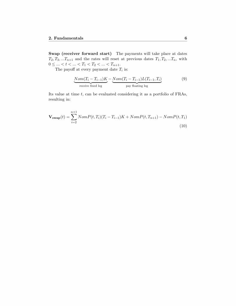
Swap (receiver forward start) The payments will take place at datesT2, T3, ...Tn+1 and the rates will reset at previous dates T1, T2, ...Tn, with0 ≤ ... < t < ... < T1 < T2 < ... < Tn+1.
The payoff at every payment date Ti is:
Nom(Ti − Ti−1)K︸ ︷︷ ︸receive fixed leg
−Nom(Ti − Ti−1)L(Ti−1, Ti)︸ ︷︷ ︸pay floating leg
(9)
Its value at time t, can be evaluated considering it as a portfolio of FRAs,resulting in:
Vswap(t) =
n+1∑i=2
NomP (t, Ti)(Ti − Ti−1)K +NomP (t, Tn+1)−NomP (t, T1)
(10)

2. Fundamentals 7
2.2 No-arbitrage pricing in continuous time
The basic tools that will be required for valuation purposes will be outlined.We will start with several definitions and results from [Musiela and Rutkowski, 1997]that will set the stage for the statement of the most important result in theSection, the Fundamental Pricing Equation.
Q ∼ P is a martingale measure ⇐⇒ S(t)
B(t)is a Q - local martingale (11)
with S(t) being a tradable asset.
Q ∼ P is a spot martingale measure ⇐⇒Vφ(t)
B(t)is a Q - local martingale
(12)for every self financing trading strategy φ. 2
The interesting result is that, under no dividends paid by the underlying,(11) ⇐⇒ (12), that is
S(t)
B(t)is a Q - local martingale ⇐⇒
Vφ(t)
B(t)is a Q - local martingale (13)
so by finding an equivalent measure under which the tradable asset dividedby a numeraire is a (local) martingale, we have automatically found a mea-sure that also makes a (local) martingale the discounted value process of aself financing trading strategy.
Fundamental pricing equation Consider a self-financing portfolio, witht value V (t), that replicates an FT -measurable claim C. Then, the time tprice of the claim πC(t) has to verify:
πC(t) = V (t) ∀t (14)
or else there exists an arbitrage opportunity.3
2We will assume that it satisfies any of the sufficient conditions in [Protter, 2003] to be amartingale. [Musiela and Rutkowski, 1997] address this issue by working with admissible
strategies, defined as those whose discounted values V (t)B(t)
follow martingales under Q.3This is clearly a situation that every valuation model has to forbid in order to be
economically sound. An arbitrage opportunity is an strategy such that:
• V (0) = 0
• V (T ) ≥ 0
• E[V (T )] > 0
2. Fundamentals 8
Under the martingale measure, V (t)B(t) is a martingale (see (13)) so it holds
that:V (t)
B(t)= EQ
[V (T )
B(T )|Ft]
(15)
As the existence of an equivalent martingale measure Q rules out arbi-trage opportunities,4 we can combine (14) and (15), and the fact that for areplicating strategy V (T ) = C, to state:
πC(t) = V (t) = B(t)EQ
[C
B(T )|Ft]
(16)
The martingale measure plays therefore a crucial role, both forbiddingarbitrage and allowing us to price a claim just by finding and expectation,rather than trying to figure out the composition of the portfolio strategy(the hedge portfolio, also of interest, should be found by other means).
Change of measure A practical statement of Girsanov’s theorem appliedto Brownian Motion, based on [Baxter and Rennie, 1996] is:
W (t) is a P-Brownian motion, and γ(t) is and adapted process satisfyingthe Novikov5 condition
=⇒
there exists a probability measure Q ∼ P, such that W (t) := W (t)+∫ t
0 γ(s)ds
is a Q-Brownian motion (in differential notation, we write dW (t) = dW (t) +γ(t)dt ).
So under certain conditions, we can manipulate by a change of measurethe drift of a process, obtaining when possible the desired driftless dynamicsrequired for the martingale measure in (11) .
4This important result is sometimes referred to as the First Fundamental Theo-rem of Asset Pricing. The proof in a intuitive discrete-time setting can be found in[Pliska, 1997], its continuous-time analogue, however, poses some challenges, as discussedin [Musiela and Rutkowski, 1997] or [Sondermann, 2006]. We don’t delve into any detailand assume that the Theorem holds for all relevant situations.
5Novikov condition, i.e. EP
[exp
(12
∫ T0γ2(s)ds
)]< ∞, is a a sufficient condition for
E(γ)(t) to be a martingale and to define a probability measure via E(γ) = dQdP .

2. Fundamentals 9
2.3 [Heath et al., 1992] framework: No-arbitrage condition
We briefly review the no-arbitrage condition in the Heath-Jarrow-Mortonsetup of [Heath et al., 1992]. The exposition is based on the notes of [Cairns, 2004]and [Baxter and Rennie, 1996]. We concentrate on the situation wheref(t, T ) is driven by one factor for clarity’s sake, although we will be dealingwith a two-factor model in Section 5.
In this framework, the instantaneous forward rate is modeled under P as:
f(t, T ) = f(0, T ) +
∫ t
0α(u, T )du+
∫ t
0σ(u, T )dW (u) (17)
where, with fixed T , α(t, T ) and σ(t, T ) are adapted processes in time t.The initial forward curve f(0, T ) is assumed to be known. Therefore, for afixed T , f(t, T ) is a process satisfying6:
dtf(t, T ) = α(t, T )dt+ σ(t, T )dW (t) (18)
Money market account From equations (8), (17) and (7) we have:
B(t) = exp
(∫ t
0r(s)ds
)= exp
(∫ t
0
[f(0, s) +
∫ s
0α(u, s)du+
∫ s
0σ(u, s)dW (u)
]ds
)And changing the order of integration on both double integrals: 7
B(t) = exp
(∫ t
0f(0, s)ds+
∫ t
0
∫ t
uα(u, s)dsdu+
∫ t
0
∫ t
uσ(u, s)dsdW (u)
)Zero-coupon bond By equation (6) and again changing order of integra-tion:
P (t, T ) = exp
(−∫ T
tf(t, s)ds
)= exp
(−∫ T
tf(0, s)ds−
∫ t
0
∫ T
tα(u, s)dsdu−
∫ t
0
∫ T
tσ(u, s)dsdW (u)
)6Subindex t included to remark the fact that f(t, T ) is a process over time t.7Some technical conditions are required for changing the order of integration on
both Riemann and Ito integrals, they are included in the assumptions made by[Heath et al., 1992] . The statement of the Fubini-style result for stochastic integralscan be found in [Filipovic, 2009].
2. Fundamentals 10
We are interested in the discounted asset dynamics Z(t) in order to definea measure Q under which Z(t) is a martingale.
Discounted zero-coupon bond The discounted bond can be computedas:
Z(t, T ) :=P (t, T )
B(t)
= exp
(−∫ T
0f(0, s)ds−
∫ t
0
∫ T
uα(u, s)dsdu−
∫ t
0
∫ T
uσ(u, s)dsdW (u)
)It is convenient to set8:
Σ(u, T ) := −∫ T
uσ(u, s)ds (19)
So we write:
Z(t, T ) = exp
(−∫ T
0f(0, s)ds−
∫ t
0
∫ T
uα(u, s)dsdu+
∫ t
0Σ(u, T )dW (u)
)Its dynamics can be computed setting Z(t, T ) := exp (Y (t, T )) and ap-
plying Ito’s lemma:
dtZ(t, T ) = Z(t, T )dY (t, T ) +1
2Z(t, T )d〈Y, Y 〉t
= Z(t, T )
[(∫ T
tα(t, s)ds
)dt+ Σ(t, T )dW (t)
]+
1
2Z(t, T )Σ2(t, T )dt
= Z(t, T )
[[(∫ T
tα(t, s)ds
)+
1
2Σ2(t, T )
]dt+ Σ(t, T )dW (t)
]= Z(t, T )Σ(t, T )
[dW (t) +
(1
2Σ(t, T )− 1
Σ(t, T )
∫ T
tα(t, s)ds
)dt
]Considering γ(t) := 1
2Σ(t, T ) − 1Σ(t,T )
∫ Tt α(t, s)ds, we can apply Gir-
sanov’s theorem to define an equivalent probability measure Q under which:
W (t) := W (t)+
∫ t
0γ(u)du = W (t)+
∫ t
0
1
2Σ(u, T )− 1
Σ(u, T )
(∫ T
uα(u, s)ds
)du
is a Q-Brownian motion.
8We will see later that this expression can be interpreted as the bond price volatility.
2. Fundamentals 11
The discounted bond dynamics under Q become:
dtZ(t, T ) = Z(t, T )Σ(t, T )dW (t) (20)
so Z(t, T ) is, up to a technical condition, a Q-martingale.Rearranging the expression for γ(t):
−γ(t)Σ(t, T ) +1
2Σ(t, T )2 =
∫ T
tα(t, s)ds (21)
Differentiating both sides with respect to T (applying Leibniz’s integralrule) and rearranging we obtain:
α(t, T ) = γ(t)σ(t, T )− Σ(t, T )σ(t, T ) = σ(t, T )[γ(t)− Σ(t, T )] (22)
With this relationship, that implies absence of arbitrage by the existenceof Q, we can now go back to the instantaneous forward rate P-dynamics (18)and apply (22):
dtf(t, T ) = α(t, T )dt+ σ(t, T )dW (t)
= σ(t, T )[γ(t)− Σ(t, T )]dt+ σ(t, T )dW (t)
= σ(t, T )[dW (t) + γ(t)dt︸ ︷︷ ︸dW (t)
−Σ(t, T )]dt]
= −Σ(t, T )σ(t, T )dt+ σ(t, T )dW (t) (23)
obtaining this way the dynamics of f(t, T ) under Q.As we can see, the instantaneous forward rate Q-dynamics are fully de-
termined by the specification of σ(t, T ).
Bond dynamics under Q are easily computed using Ito’s product rulerealizing that P (t, T ) = Z(t, T )B(t):
dtP (t, T ) = dt[Z(t, T )B(t)]
= Z(t, T )Σ(t, T )dW (t)B(t) + r(t)B(t)dt Z(t, T )
= P (t, T )[r(t)dt+ Σ(t, T )dW (t)] (24)
Equation (24) is the reason why Σ(t, T ) is known as the bond pricevolatility (under Q).

2. Fundamentals 12
2.4 Forward measure
The concept of change of numeraire will be thoroughly used in later Sections,so we proceed to describe the basics.
Numeraire Based on the exposition by [Privault, 2018] a suitable nu-meraire N(t) needs to verify:
1. N(t) > 0 ∀t
2. N is not a dividend paying asset
3. N(t)B(t) is a Q-martingale
with Q representing the measure associated with the money market accountnumeraire B(t).
Forward measure Given a numeraire N(t), the forward measure P isdefined through the Radon-Nikodym derivative as:
dPdQ
:=
N(T )N(0)
B(T )B(0)
=N(T )
N(0)
1
B(T )(25)
Applicability of the forward measure [Brigo and Mercurio, 2006] enun-ciate a wider version of the result, but for our needs it is enough to state:
S(t)
B(t)is a martingale under Q⇒ S(t)
N(t)is a martingale under P as defined in (25)
Forward measure with zero-coupon bond numeraire In our analy-sis, the zero-coupon bonds (for different maturities) will be our assets, anda zero-coupon bond as well, but with a fixed maturity, our numeraire 9.
The fact that P (T, T ) is equal to 1, in contrast to B(T ), which needsinformation up to T to be known, makes convenient the use of the zero-coupon bond as a numeraire.
9The zero-coupon bond is indeed a suitable numerarie: it is reasonable to assume thatits value, even in the worst scenario, is always greater than zero. Also it doesn’t haveintermediate payments and as seen in (20), it is a Q-martingale when divided by themoney market account.
2. Fundamentals 13
We proceed to set N(t) := P (t, T ), and consider another bond P (t, U)as the asset, with U > T . The bond price discounted by our new numeraire,should be a martingale under PT , so we will look for an appropriate changeof measure,10 setting:
Y (t, U) :=P (t, U)
P (t, T )
Recalling the dynamics of the bond price under Q (see (24)), and usingIto’s product rule, the dynamics of Y (t, U) are:
dtY (t, U) = Y (t, U)(Σ(t, U)−Σ(t, T ))dW (t)+Y (t, U)Σ2(t, T )dt−Y (t, U)Σ(t, U)Σ(t, T )dt
Rearranging terms to clearly see the shape of the γT (t)11 required toobtain driftless dynamics:
dtY (t, U) = Y (t, U)(Σ(t, U)− Σ(t, T ))
[dW (t)
+Σ2(t, T )
Σ(t, U)− Σ(t, T )dt− Σ(t, U)Σ(t, T )
Σ(t, U)− Σ(t, T )dt
]= Y (t, U)(Σ(t, U)− Σ(t, T ))
[dW (t)− Σ(t, T )[Σ(t, T )− Σ(t, U)]
Σ(t, T )− Σ(t, U)dt
]= Y (t, U)(Σ(t, U)− Σ(t, T ))
[dW (t)− Σ(t, T )dt
]Setting γT (t) := −
∫ t0 Σ(s, T )ds and assuming that the required technical
conditions hold, we can use Girsanov’s theorem again to define an equivalentprobability measure PT such that:
dW T (t) = dW (t)− Σ(t, T )dt (26)
is a PT -Brownian motion.
Finally, applying (26) we get the sought driftless dynamics:
dtY (t, U) = Y (t, U)(Σ(t, U)− Σ(t, T ))dW T (t)10The steps followed here are found in [Cairns, 2004], which seem the most intuitive
for justifying the form of the forward measure with bond numeraire; first computing thediscounted dynamics, and then defining a change of measure that will make it a (local)martingale under the new measure.
11We include a T subindex on γ(t) to remark the dependence of the particular maturityof the bond used as numeraire.

2. Fundamentals 14
Conditional expectation under PT and the Fundamental PricingEquation [Privault, 2018] shows that:
dPFtdQFt
=B(t)
B(T )
N(T )
N(t)
Then, for any FT -measurable payoff C:
EQ
[B(t)
B(T )C|Ft
]= EQ
[B(t)
B(T )
N(t)
N(t)
N(T )
N(T )C|Ft
]= EQ
[dPFtdQFt
N(t)
N(T )C|Ft
]
= EP
[N(t)
N(T )C|Ft
](27)
Considering the zero-coupon bond numeraire, the result in (27) becomes:
EQ
[B(t)
B(T )C|Ft
]= EP
[P (t, T )
P (T, T )C|Ft
]= EP [P (t, T )C|Ft]
So we have arrived at the relation:
B(t)EQ
[1
B(T )C|Ft
]= P (t, T )EP [C|Ft] (28)
where the left-hand side corresponds to the Fundamental Pricing Equation(16).
3. Valuation of interest rate derivatives: General results 15
3 Valuation of interest rate derivatives: Generalresults
The valuation of several interest rate derivatives will be outlined here, ob-taining expressions that will be used in Section 7. We set the nominal ofevery instrument to 1 (Nom := 1) to make the exposition simpler.
3.1 Vanilla caplet
For a vanilla caplet with strike k, settle date T1 and maturity T2, the payoffis defined as:
δ(F (T1, T1, T2)− k)+ = δ(L(T1, T2)− k)+
being the payoff FT1-measurableBy the fundamental pricing equation (16):
Vcaplet(t) = B(t)EQ
[1
B(T2)δ(L(T1, T2)− k)+|Ft
]= EQ
[exp
(−∫ T2
tr(s)ds
)δ(L(T1, T2)− k)+|Ft
]Making use of iterated conditioning on FT1 and noticing the fact that
P (T1, T2) = EQ
[exp
(−∫ T2T1r(s)ds
)|FT1
], we get:
Vcaplet(t) = EQ
[exp
(−∫ T1
tr(s)ds
)P (T1, T2)δ[L(T1, T2)− k]+|Ft
]= EQ
[exp
(−∫ T1
tr(s)ds
)P (T1, T2)δ
[1
δ
(1
P (T1, T2)− 1
)− k]+
|Ft
]
Multiplying by1 + kδ
1 + kδand defining K ′ :=
1
1 + kδ:
Vcaplet(t) = 1 + kδ︸ ︷︷ ︸1K′
EQ
exp
(−∫ T1
tr(s)ds
) 1
1 + kδ︸ ︷︷ ︸K′
−P (T1, T2)
+
|Ft
We can see that this last expression is just 1
K′ times the t price of a putoption with strike K ′ and maturity T1 written on the bond P (T1, T2).
3. Valuation of interest rate derivatives: General results 16
The computation of the expectation can be simplified by means of achange of measure as noted in Section 2.4. Using (28), we get the finalexpression for the value of a vanilla caplet:
Vcaplet(t) =1
K ′EQ
[exp
(−∫ T1
tr(s)ds
)[K ′ − P (T1, T2)
]+|Ft]=
1
K ′P (t, T1)EPT1
[[K ′ − P (T1, T2)
]+|Ft] (29)
3.2 Barrier caplet
As an example of a path-dependent derivative, we consider a barrier down-and-out caplet with strike k, settle date T1 and maturity T1 + δ over theδ-period simple spot rate with barrier level B. The payoff of such instrumentis:
δ
(L(T1, T1 + δ)− k
)+
1{τB > T1}
withτB := inf {ti | L(ti, ti + δ) < B} (30)
so τB represents the first moment the time-ti simple forward rate falls belowthe barrier level. The expression {τB > T1} states that the crossing eventhappens after the expiry of the option (so, for valuation purposes, the un-derlying does not cross the barrier and the indicator function takes value1).
Being 1{τB > T1} an FT1 measurable random variable, we can use ananalogous procedure to the previous one to value the barrier caplet, obtain-ing:
Vbarriercaplet(t) =1
K ′P (t, T1)EPT1
[[K ′ − P (T1, T2)
]+1{τB > T1}|Ft
](31)
3.3 European swaption
Considering the swap defined in Section 2.1, its value at T1 (noting (10)) is:
Vswap(T1) =
n+1∑i=2
P (T1, Ti)(Ti − Ti−1)K + P (T1, Tn+1)− P (T1, T1)

3. Valuation of interest rate derivatives: General results 17
The option (European swaption) to enter the swap at T1 with strike Khas a T1 payoff of:(
K
n+1∑i=2
P (T1, Ti)(Ti − Ti−1) + P (T1, Tn+1)− 1
)+
(32)
Again, applying the fundamental pricing equation (16) over the payoff (32),we get:
VESwaption(t) = EQ
B(t)
B(T )
(K
n+1∑i=2
P (T1, Ti)(Ti − Ti−1) + P (T1, Tn+1)− 1
)+
|Ft
And finally, under PT1 :
VESwaption(t) = P (t, T )EPT1
(K n+1∑i=2
P (T1, Ti)(Ti − Ti−1) + P (T1, Tn+1)− 1
)+
|Ft
(33)
3.4 Bermudan swaption
American-style derivatives introduce a layer of complexity over the previousinstruments, and cannot be handled directly with the fundamental pricingequation. Here we just formulate the problem here in Section 7 we willexplore numerical procedures to approximate the value of the option.
Following [Glasserman, 2003] and considering the payoff in (32) the valueof the Bermudan option at t = 0 maturing at T1 is:
VBSwaption(0) = supτ
EQ
exp
(∫ τ
0r(s)ds
)(K
n+1∑i=2
P (τ, Ti)(Ti − Ti−1) + P (τ, Tn+1)− 1
)+
where the supτ represents the computation of the supremum over the set ofexercise strategies τ taking values in [0, T1].
Again, by a change of measure and applying (28):
VBSwaption(0) = supτ
P (0, τ)EPT1
(K n+1∑i=2
P (τ, Ti)(Ti − Ti−1) + P (τ, Tn+1)− 1
)+

4. [Cheyette, 1994] approach: Justification and modelspecification 18
4 [Cheyette, 1994] approach: Justification and modelspecification
An adapted process X(t) is Markov if
E[h(X(u))|Ft] = E[h(X(u))|Xt], ∀ 0 ≤ t ≤ u
A more practical statement about the Markov property is found in[Protter, 2003], where it is stated that (under certain technical conditions),a process with differential:
dX(t) = h(X(t), t)dt+ g(X(t), t)dW (t) (34)
with h and g being functions of X(t) and t, is a Markov process.In the Heath-Jarrow-Morton setting, the instantaneous short rate is:
r(t) = f(t, t) = f(0, t) +
∫ t
0α(u, t)du+
∫ t
0σ(u, t)dW (u)
Focusing on the second integral:
A(t) :=
∫ t
0σ(u, t)dW (u)
This process has differential dA(t) = σ(t, t)dW (t)+
(∫ t0∂σ(u,t)∂t dW (u)
)dt
so, in general, cannot be written in the form of (34) and therefore is notMarkovian. This has attracted some research and several authors have spec-ified conditions where the Markovianity is preserved.12.
In this Thesis, we follow the work of [Cheyette, 1994], however, we willrestrict ourselves to the specification used by [Beyna, 2013] where the func-tions for the instantaneous forward rate volatility are deterministic in orderto work on a gaussian Heath-Jarrow-Morton environment, therefore exclud-ing stochastic volatility or dependence on the instantaneous forward rate.13
12For example in [Ritchken et al., 1995], they are able to express a one factor Heath-Jarrow-Morton structure as a two-state variables Markov process by imposing:
σf (t, T ) = σr exp
(−∫ T
t
κ(u)du
).
13The results in [Cheyette, 1994] allow for the use of non-deterministic volatility func-tions σ(t, T, ω) while still preserving Markovianity.
4. [Cheyette, 1994] approach: Justification and modelspecification 19
4.1 Cheyette-Beyna model specification
The specification for each volatility function is as follows:14
σk(t, T ) :=
Nk∑i=1
αik(T )
αik(t)βik(t), k = 1, 2...M (35)
The total number of summands∑M
k=1Nk of each function through allfunctions determines the number of state variables in the model15.
An interesting feature is that the function β(t) can be set to a polynomialof any order without increasing the complexity of the model in terms offactors or state variables, because it does not add additional summands inthe volatility functions in (35).
The model relies on the definition of the state variables Xij(t). Otherprocesses have to be defined as well:
Auxiliary processes
Aik(t) :=
∫ t
0αik(s)ds (36)
14This specification nests some popular models. For example, Ho-Lee model in Heath-Jarrow-Morton specification reads:
σ(t, T ) := σ
Which can be achieved in Cheyette form by setting:
α11(t) := 1
β11(t) := σ
M := 1
N1 := 1
So we obtain:
σ1(t, T ) =
1∑i=1
α11(T )
α11(t)β11(t) =
1
1σ = σ
15Not to confuse with the number of factors M, related to the number of independentBrownian motions in the specification of the instantaneous forward rate dynamics.
4. [Cheyette, 1994] approach: Justification and modelspecification 20
Quadratic variation processes 16
Vij,k(t) :=
∫ t
0
αik(t)αjk(t)
αik(s)αjk(s)βik(s)βjk(s)ds = Vji,k(t) (37)
State variables Using the previous definitions, we set:
Xik(t) :=
∫ t
0
αik(t)
αik(s)βik(s)dWk(s)+
∫ t
0
αik(t)
αik(s)βik(s)
Nk∑j=1
Ajk(t)−Ajk(s)αjk(s)
βjk(s)
ds
(38)
Dynamics of the state variables The dynamics under Q are shown in[Beyna, 2013] to be:17
dXik(t) =
Xik(t)∂
∂t(logαik(t)) +
Nk∑j=1
Vij,k(t)
dt+ βik(t)dWk(t) (39)
These state variables are indeed Markov processes (i.e., they verify (34))so the model can be expressed as a Markovian system.18
We can now determine the form of the fundamental interest rate mod-eling elements within the model.
Instantaneous forward rate Inserting (35) in (17), and considering the-newly defined (36), (37) and (38), the instantaneous forward rate under Qcan be expressed as:
f(t, T ) = f(0, T )+
M∑k=1
Nk∑j=1
αjk(T )
αjk(t)(Xjk(t) +
Nk∑i=1
Aik(T )−Aik(t)αik(t)
Vij,k(t))
(40)
A detailed derivation for our particular model (to be specified in Section5), based on [Beyna, 2013], is presented in Appendix A.1.
16This terminology is used because the quadratic variation processes of X11(t) andX12(t) coincide with V11,1(t) and V11,2(t) respectively.
17We include a commented reproduction of the computations in Appendix B due to theimportance of this result and the presence of some errata in Beyna’s material.
18For instance, the short rate is now Markovian as it can be expressed as the sum ofthe state variables:
r(t) = f(0, t) +
M∑k=1
Nk∑j=1
Xjk(t)
4. [Cheyette, 1994] approach: Justification and modelspecification 21
Zero-coupon bonds The formula for bonds can be explicitly computed(as shown in [Cheyette, 1994] and [Beyna, 2013]) using (6) and (40). Aftersome calculations we get:19
P (t, T ) = exp
(−∫ T
tf(t, u)du
)
= exp
−∫ T
tf(0, u) +
M∑k=1
Nk∑j=1
αjk(u)
αjk(t)(Xjk(t) +
Nk∑i=1
Aik(u)−Aik(t)αik(t)
Vij,k(t)
du
=
P (0, T )
P (0, t)exp
(−
M∑k=1
Nk∑j=1
Ajk(T )−Ajk(t)αjk(t)
Xjk(t)
−M∑k=1
Nk∑i=1
Nk∑j=1
[Ajk(T )−Ajk(t)][Aik(T )−Aik(t)]2αik(t)αjk(t)
Vij,k(t)
)(41)
Equation (41) provides the link between state variables and bond prices,for this reason, it will be extensively used in Section 7.
19The details justifying second equality, following [Beyna, 2013], can be found for ourmodel in Appendix A.2.

5. Two-factor Cheyette model 22
5 Two-factor Cheyette model
The particular model within the Cheyette-Beyna environment that will beanalyzed in the rest of the Thesis is defined here. We try to find an speci-fication simple enough so the computations in the last Section are straight-forward but that still maintains a reasonable degree of flexibility. In hiswork, [Beyna, 2013] proposes a Three-factor version based on exponentialvolatility functions that turns out to be too cumbersome in calculations.After some trials, a simplified version of the HJM G2++ of [Acar, 2009] ischosen, where the exponential function of the first factor is replaced with aconstant.
5.1 Specification
The model includes a second factor (M := 2) independent of the first. Then,we may specify the following in Cheyette-Beyna form, withN1 := 1, N2 := 1:
α11(t) := 1 (42a)
β11(t) := a (42b)
α12(t) := exp (−θt) (42c)
β12(t) := c (42d)
The model involves two factors and also two state variables. The volatil-ity functions turn into:
σ1(t, T ) =
1∑i=1
αi1(T )
αi1(t)βi1(t) =
1
1a = a (43a)
σ2(t, T ) =
1∑i=1
αi2(T )
αi2(t)βi2(t) =
exp (−θT )
exp (−θt)c = exp [−θ(T − t)]c (43b)
The parameters should verify the constraint imposed by the requiredpositivity of the volatility functions, i.e. σk(t, T ) > 0 k = 1, 2. In this case,our model contains three parameters: a, c ∈ R+ and θ ∈ R.
Now we have to evaluate (36), (37) and (38), with our particular choiceof volatility functions defined in (42a) through (42d).

5. Two-factor Cheyette model 23
First obtaining the auxiliary processes:
A11(t) =
∫ t
01ds = t
A12(t) =
∫ t
0exp (−θs)ds = −1
θ[exp (−θt)− 1]
Then, evaluating Vij,k(t):
V11,1(t) =
∫ t
0a2ds = a2t
V11,2(t) =
∫ t
0
exp (−θt) exp (−θt)exp (−θs) exp (−θs)
c2ds =c2
2θ
[1− exp (−2θt)
]And also computing the state variables under Q:
X11(t) =
∫ t
0adW1(s) +
∫ t
0a [(t− s)a] ds =
∫ t
0adW1(s) +
1
2a2t2 (44)
X12(t) =
∫ t
0
exp (−θt)exp (−θs)
c dW2(s)
+
∫ t
0
exp (−θt)exp (−θs)
c
(−1θ [exp (−θt)− 1] + 1
θ [exp (−θs)− 1]
exp (−θs)c
)ds
= c exp (−θt)∫ t
0exp (θs)dW2(s)
+ c2 exp (−θt)1
θ
∫ t
0exp (2θs)[exp (−θs)− exp (−θt)] ds
= c exp (−θt)∫ t
0exp (θs)dW2(s) + c2 1
θ2
[1
2[exp (−2θt)− 1] + 1− exp (−θt)
]= c exp (−θt)
∫ t
0exp (θs)dW2(s) + c2
(1
2θ2− exp(−2tθ)[2 exp(tθ)− 1]
2θ2
)Having in mind the instruments studied in Section 3, we are most inter-
ested in the dynamics of the state variables under the T1-forward measure.To that regard, we first compute the bond price volatility (see (19)) for eachfactor in order to define the measure PT1 .
Bond price volatilities
Σ1(t, T1) = −∫ T1
tσ1(t, u)du = −
∫ T1
ta du = −a(T1 − t) (45)
5. Two-factor Cheyette model 24
Σ2(t, T1) = −∫ T1
tσ2(t, u)du = −
∫ T1
texp [−θ(u− t)]c du =
c
θ[exp (−θ(T1 − t))−1]
(46)We apply Multidimensional Girsanov’s theorem to define an equivalent
probability measure PT1 :
dW1(t) = dW1(t)− Σ1(t, T1)dt = dW1(t) + a(T1 − t)dt
dW2(t) = dW2(t)− Σ2(t, T1)dt = dW2(t)− c
θ[exp (−θ(T1 − t))− 1](47)
where W1(t), W2(t) are independent Brownian motions under PT1 .Applying this change of measure we can now compute the state variables
under PT1 . It will also be useful for later calculations to evaluate both statevariables at t = T1 and determine its distribution.
State variables under PT1
X11(t) =
∫ t
0a[dW PT1
1 (s)− a(T1 − s)ds] +1
2a2t2
=
∫ t
0a dW PT1
1 (s)−∫ t
0a2(T1 − s)ds+
1
2a2t2
=
∫ t
0a dW PT1
1 (s)− a2T1t+ a2t2
At t = T1,
X11(T1) =
∫ T1
0a dW PT1
1 (s)
EPT1 [X11(T1)] = 0
Applying Ito’s isometry:
VPT1 [X11(T1)] = a2T1
Due to the normal distribution of stochastic integrals of deterministicintegrands with respect to Brownian motion:
X11(T1)PT1∼ N (0, a2T1)
5. Two-factor Cheyette model 25
X12(t) = c exp (−θt)∫ t
0exp (θs)dW PT
2 (s)
+c2
θ2exp(−θt)
(1
2exp(−θT1)
(exp(2θt)− 1
)− exp (θt) + 1
)+ c2
(1
2θ2− exp(−2tθ)[2 exp(tθ)− 1]
2θ2
)At t = T1,
X12(T1) = c exp (−θT1)
∫ T1
0exp (θs)dW PT
2 (s)
EPT1 [X12(T1)] = 0
VPT1 [X12(T1)] =c2
2θ
[1− exp (−2θT1)
]
X12(T1)PT1∼ N
(0,c2
2θ
[1− exp (−2θT1)
])We compute the covariance between the state variables, applying the
polarization identity:
CovPT1 [X11(T1), X12(T1)] = CovPT1
[ ∫ T1
0a dW PT1
1 (s) ,
∫ T1
0c exp (−θT1) exp (θs)dW PT
2 (s)
]= EPT1
[ ∫ T1
0a dW PT1
1 (s) ·∫ T1
0c exp (−θT1) exp (θs)dW PT
2 (s)
]= EPT1
[ ∫ T1
0a c exp (−θT1) exp (θs) d〈W PT1
1 ,W PT2 〉(s)
]= 0
Because the driving Brownian motions are independent and the inte-grand is deterministic, they are jointly normal. As the covariance betweenthem is zero, we conclude that the two state variables are independent.
5. Two-factor Cheyette model 26
We can also compute their PT1-dynamics, combining (39) with (47):
Dynamics of the state variables under PT1
dXik(t) =
Xik(t)∂
∂t(logαik(t)) +
Nk∑j=1
Vij,k(t)
dt + βik(t)(dW T
k (t) + Σ(t, T )dt)
=
Xik(t)∂
∂t(logαik(t)) +
Nk∑j=1
Vij,k(t) + βik(t)Σ(t, T )
dt
+ βik(t)dWTk (t)
In our model, they become:
dX11(t) = a2 (2t− T1) dt + a dW PT11 (t)
dX12(t) =
(−θX12(t) +
c2
2θ
[1− exp (−2θt)
]+c2
θ
[exp (−θ(T1 − t))− 1
])dt
+ cdW PT12 (t) (48)
The zero-coupon bond price will be the reference quantity used to valuethe instruments in Section 7.
Zero-coupon bond price Using (41), we can readily compute the ex-pression for bond prices in our model:
P (t, T ) =P (0, T )
P (0, t)exp
[−(A11(T )−A11(t)
α11(t)X11(t) +
A12(T )−A12(t)
α12(t)X12(t)
)−
([A11(T )−A11(t)][A11(T )−A11(t)]
2α11(t)α11(t)V11,1(t)
+[A12(T )−A12(t)][A12(T )−A12(t)]
2α12(t)α12(t)V11,2(t)
)]
=P (0, T )
P (0, t)exp
[− (T − t)X11(t)− 1
θ
(1− exp[−θ(T − t)]
)X12(t)
− 1
2(T − t)2a2t − 1
2θ2
(1− exp[−θ(T − t)]
)2 c2
2θ
[1− exp (−2θt)
]](49)
5. Two-factor Cheyette model 27
Note that given:
• the zero coupon initial curve, T 7→ P (0, T )
• values for the parameters a, c, θ
the zero-coupon bond t price for any maturity T , is a function P (t, T,X11(t), X12(t)).The exponent happens to be the sum of independent normal random vari-ables, therefore we conclude that the bond price is lognormally distributed.
5.2 Caplet analytical formula
Being in a gaussian Heath-Jarrow-Morton setting, we can obtain a closed-form expression for caplets 20 based on the lognormal distribution of bondprices.
We start by stating the following useful result for the valuation of calloptions, found for example in [Cairns, 2004]:
Expectation of maximum of lognormal random variable minus apositive constant. If X has a lognormal distribution under a probability
measure P, that is, log (X)P∼ N
(e, d2
), then for any constant K > 0:
EP[(X −K)+
]= EP[X]Φ
(e+ d2 − logK
d
)−KΦ
(e− logK
d
)(50)
where Φ(x) denotes the standard normal cumulative density function eval-uated at x, and e := EP[logX], d2 := VP[logX].
For our purposes, X := P (T1, T2) and e = EPT1 [logP (T1, T2)], d2 =VPT1 [logP (T1, T2)]. We first compute the variance, using the previouslycomputed moments of the state variables.
20Computing unconditional expectation is enough for the purpose of valuation of claimsat t = 0 (which is what we will be doing in Section 7), and it is easier than the moregeneral moments conditional on Ft.
5. Two-factor Cheyette model 28
VPT1 [logP (T1, T2)] = VPT1
[−(A11(T2)−A11(T1)
α11(T1)X11(T1)+
A12(T2)−A12(T1)
α12(T1)X12(T1)
)]
=
(A11(T2)−A11(T1)
α11(T1)
)2
VPT1 [X11(T1)]+
(A12(T2)−A12(T1)
α12(T1)
)2
VPT1 [X12(T1)]
+ 2
(A11(T2)−A11(T1)
α11(T1)
)(A12(T2)−A12(T1)
α12(T1)
)CovPT1 [X11(T1), X12(T1)]
= (T2 − T1)2a2T1 +
(1− exp (−θ(T2 − T1))
θ
)2 c2
2θ
[1− exp (−2θT1)
](51)
A result in [Cairns, 2004] linking expectation and variance in this settingallows us to quickly compute the expectation as:
EPT1 [logP (T1, T2)|] = logP (0, T2)
P (0, T1)+
1
2VPT1 [logP (T1, T2)|] (52)
The pull-call parity for European bond options states that:
Callbond(t, T1, T2,K)−P (t, T2) +KP (t, T1) = Putbond(t, T1, T2,K) (53)
Knowing the relationship (53), we can restate the value of the capletpreviously determined in (29), in terms of the price of a call bond option sowe can apply (50):
Vcaplet(0) =1
K ′P (0, T1)EPT1
[[K ′ − P (T1, T2)
]+](54)
=1
K ′
(P (0, T1)EPT1
[[P (T1, T2)−K ′
]+]− P (0, T2) +K ′P (0, T1)
)Noting that:
EPT1 [P (T1, T2)] = EPT1
[P (T1, T2)
P (T1, T1)
]=P (0, T2)
P (0, T1)
5. Two-factor Cheyette model 29
The expectation in (54) then becomes:
EPT1
[[P (T1, T2)−K ′
]+]= EPT1 [P (T1, T2)] Φ
(e+ d2 − logK ′
d
)−K ′Φ
(e− logK ′
d
)=
P (0, T2)
P (0, T1)Φ
(e+ d2 − logK ′
d
)−K ′Φ
(e− logK ′
d
)(55)
Putting all the pieces together, we arrive at:
Vcaplet(0) =1
K ′
(P (0, T1)
[P (0, T2)
P (0, T1)Φ
(e+ d2 − logK ′
d
)
− K ′Φ
(e− logK ′
d
)]− P (0, T2) +K ′P (0, T1)
)
=1
K ′
(P (0, T2)Φ
(e+ d2 − logK ′
d
)
− K ′P (0, T1)Φ
(e− logK ′
d
)− P (0, T2) +K ′P (0, T1)
)(56)
where e = EPT1 [logP (T1, T2)] and d2 = VPT1 [logP (T1, T2)] have beencomputed in (51) and (52).
The analytical formula obtained is convenient for the calibration proce-dure that will be explained in Section 6 and for the implementation of acontrol variate estimator in Section 7.

6. Calibration. Simulated annealing 30
6 Calibration. Simulated annealing
The process of adjusting model parameters to market reality is known ascalibration. There exist several approaches to it and usually only a frac-tion of the market is considered. In order to calibrate the proposed modelto market transactions, we choose a somewhat simplified approach whereonly OIS rates and a set of EUR caps with a particular strike will betaken into account.21 We consider a set of market caplet prices22 withstrike k = 0.005, settle dates {0.25, 0.5, 0.75, ..., 28.5, 29, 29.5} and maturi-ties {0.5, 0.75, 1, ..., 29, 29.5, 30}. We have a total of 63 prices that can bearranged in a vector capletsMKT63×1.
The process is meant to find parameters that minimize the sum ofsquared errors, SSE, between market and model prices23 under said pa-rameters.
The minimization procedure will be achieved using a simulated anneal-ing routine. It is a derivative-free optimization method whose adequacy formodels of this class is hinted at in [Beyna, 2013]. Given an initial point,the general structure involves searching randomly for neighbouring pointswhich offer a lower value of the objective function, while also introducinga probability (determined by the difference in the objective function and aparameter called temperature) of going to a worse point, which gives theprocedure the ability of not getting stuck at a local minimum.
The main elements of the procedure are:
• Objective function f (SSE in our case). The change in the value off , when evaluated in another point, is noted as Λ.
• Acceptance function, which will define the probability of accepting aworse point, that is, a point which increases the value of the objectivefunction when compared to the previous point (Λ > 0).
21We take a simplified route calibrating the models to caps of a particular strike, insteadof a more complex approach using several strikes of caps and including swaptions.
22The procedure to obtain such prices and the particularities of the EUR cap marketare treated in Appendix C.
23Some authors [Beyna, 2013] recommend calibration to implied volatilities, as they arenot as affected by maturity and strike effects, but for the sake of brevity we have not takenthat path. It is also worth noting that ATM volatility is usually the preferred choice dueto its liquidity but we did not recover it in the stripping process.
6. Calibration. Simulated annealing 31
A popular choice is the negative exponential function exp ( −ΛTemp),24
which assigns greater probability when the temperature is high and/orthe change in the objective function is small.
• Initial and final temperature, T0 and Tmin
• Temperature reduction parameter, λ
• Neighbour selection, in our case through a N (0, 1) extraction, so val-ues around 0 are more likely than extreme ones, without completelyexcluding the possibility of large numbers being obtained. A scale fac-tor allows to adjust the variance of the normal random extractions soit can better fit the magnitude of the parameters.
The implementation 25 used here is inspired on [Press et al., 2007]. Theannealing schedule will be reset M times, and the search of new points ineach temperature is repeated N times, storing the best point found so far.Also, bounds for the values of the parameters are incorporated to make surethey verify a, c ∈ R+.
Defining a function caplets2Fac(a, c, θ), that, taking the model param-eters as input, returns a vector63×1 with the Cheyette-Two-Factor modelprices for caplets with the same set of settle dates, maturities and strikeas the ones in the market (using (56)), we can set the following procedure,detailed in pseudocode in Algorithm 1.
After some experimentation, taking Temp0 = 0.01, p0 = (0.35︸︷︷︸a
0.25︸︷︷︸c
0.05︸︷︷︸θ
),
λ = 0.95, M=5, N=50, Tempmin = 0.0001, scale = 0.0001 and parameterbounds (0,∞),(0,∞),(−∞,∞), yields the results:
aopt = 0.506898, copt = 0.083819, θopt = 0.104966
SSE(aopt, copt, θopt) = 0.01495
The goodness of fit of the results can be seen in Figure 1, comparingmarket and model prices26:
24It is indeed a negative exponential function because Temp > 0, and Λ > 0 when theacceptance function is relevant. This also implies that its resulting value is never greaterthan 1, so it can be rightfully interpreted as a probability.
25The random numbers required here and in the Valuation section have been obtainedusing Matlab 2019a implementation of the Mersenne Twister algorithm for U(0, 1) variatesand the Ziggurat algorithm for obtaining N (0, 1) distributed numbers.
26An alternate calibration output was found where shorter maturities were nicely ad-justed at the expense of a high error in longer maturities. Although it might have beenan alternative in view of the instruments of Section 7, it was discarded due to the highresulting output of the SSE function.

6. Calibration. Simulated annealing 32
Figure 1: Differences between caplet market prices and caplet prices in theTwo-Factor Cheyette model with parameters a = 0.506898, c = 0.083819,θ = 0.104966.
The values found for the parameters allow us to define the volatilityfunctions:
σ1(t, T ) := 0.506898
σ2(t, T ) := exp
(− 0.104966(T − t)
)0.083819
Model specification also requires f(0, T ), which is obtained through thesplines that describe the yield curve based on market data and relations (1)and (5)27.
In the next section we assume that model parameters {a, c, θ} as well asf(0, T ) are known, so the volatility functions σ1(t, T ), σ2(t, T ) are explicitlydefined and bond prices at t = 0 are known for every possible maturity.
27See Appendix C for details, where the function T → P (0, T ) is computed using cubicsplines and relation (1). Considering (5), it is equivalent to defining the initial instanta-neous forward curve f(0, T ).

6. Calibration. Simulated annealing 33
Algorithm 1 Minimization of sum of squared model errors respect to capletmarket prices using Simulated Annealing
Require: capletsMKT , caplets2Fac(a, c, θ), Temp0, p0, α, M , N ,Tempmin, scale
Ensure: aopt, copt, θopt, f(popt)1: f(p) = (capletsMKT − caplets2Fac(p))
′ · (capletsMKT − caplets2Fac(p)). SSE function
2: pbest = p0
3: for m = 1 to M do . M resets of the annealing schedule4: Temp = Temp0
5: pold = pbest6: while Temp > Tempmin do7: for n = 1 to N do . N explorations at each temperature8: element = Select at random an element of the vector9: pold[element] = pold[element] + scale ∗ randomN (0,1)
10: if pold[1] < 0 then . Ensure a, c ∈ R+
11: pold[1] = |randomN (0,1)|12: else if pold[2] < 0 then13: pold[2] = |randomN (0,1)|14: end if15: pnew = pold16: Λ = f(pnew)− f(pold)17: if Λ < 0 then . Accept better point18: pold = pnew19: else . Accept worse point with probability prob
20: prob = exp
(−∆
Temp
)21: if randomU(0,1) < prob then22: pold = pnew23: end if24: end if25: if f(pnew) < f(pbest) then . Store best point found26: pbest = pnew27: end if28: end for n29: Temp = λ ∗ Temp . Decrease temperature30: end while31: end for m32: popt = pbest; aopt = popt[1]; copt = popt[2]; θopt = popt[3]; f(popt)33: return aopt, copt, θopt, f(popt)

7. Valuation of interest rate derivatives: Numerical methods 34
7 Valuation of interest rate derivatives: Numeri-cal methods
In this Section, we choose specific examples of the derivatives analyzed inSection 3, as a means to explain and test several numerical methods. Asuitable method will be used for each derivative and its t = 0 value will becalculated.
The chosen instruments are:
• Barrier down-and-out caplet over the 3-month simple spot rate (i.e.L(t, t + δ) with δ := 0.25), settled at T1 := 1, maturing at T2 = 1.25,with strike k = 0.005 and barrier set at B = −0.15.
• European swaption, maturing at T1 := 1 for entering a receiver swapat K = 0.005 with reset dates {1, 1.25, 1.5, 1.75} and payment dates{1.25, 1.5, 1.75, 2}.
• Bermudan swaption, for entering a receiver swap at K = 0.005 withthe same tenor structure as the previous one and possible exercisedates {0.25, 0.5, 0.75, 1}.
7.1 Monte Carlo path simulation with control variate. Bar-rier caplet
In order to simulate paths of the underlying, we implement a first orderdiscretization (Euler scheme). Because of the functional form of βik(t) ,thediffusion term never depends on X(t) , so the more precise Milstein schemecollapses into Euler scheme in the Cheyette-Beyna specification we are work-ing with. The main advantage of discretization schemes is their generality,although they introduce discretization error, so in the case of the vanillacaplet, we will test the results against known caplet analytical values tocheck their adequacy.
We will partition the interval [0, T1] in Nint = 1000 subintervals. Eachone will have the same length, namely T1
Nint, and Nint + 1 time points will
be defined 0 = t0 < t1 < ... < tNint−1 < tNint = T1 .

7. Valuation of interest rate derivatives: Numerical methods 35
The scheme for the two state variables, given the dynamics (48), is then:
X11(t0) = X11(0) = 0
X11(ti+1) = X11(ti) + a2 (2ti − T1) ∆t + a√
∆tZ1i+1
X12(t0) = X12(0) = 0
X12(ti+1) = X12(ti) +
(− θX12(ti) +
c2
2θ
[1− exp (−2θti)
]+
c2
θ
[exp (−θ(T1 − ti))− 1
])∆t + c
√∆tZ2
i+1 (57)
for i = 0, 1, ..., Nint − 1, where Z1iiid∼ N (0, 1) , Z2
iiid∼ N (0, 1) are also
independent with respect to each other.
Vanilla caplet As a reference, we compute the value of a caplet withthe same characteristics as the barrier caplet except for its barrier feature.Recalling (29), we write:
Vcaplet(0) = EPT1
[1
K ′P (0, T1)
[K ′ − P (T1, T2)
]+](58)
Applying the discretization scheme in (57) we are able to obtain real-izations of the state variables at T1. The payoff is a function of the bondprice P (T1, T2), which is itself a function of X11 and X12, and therefore itcan be computed for each realization using (49). Then we can estimate theexpectation in (58) by calculating their sample mean,28 obtaining the resultsshown in Table 1.
28We are considering the sample mean of the n independent simulations as the estimatorof the expectation. By the Central Limit Theorem, the error of the estimation is normally
distributed Vn − V ∼ N(
0,σ2V
n
), so its standard deviation is
σV√n
. Substituting σV for
the sample standard deviation sV =
√1
n− 1
∑ni=1(Vi − Vn)2, allows us to compute the
Error shown in the Table.

7. Valuation of interest rate derivatives: Numerical methods 36
Monte Carlo SimulationAnalytical
n = 100 n = 1000 n = 10000
Value 0.0535 0.0498 0.0508 0.0504sV 0.0771 0.0699 0.0645 -Error ( sV√
n) 0.0077 0.0022 0.0006 -
Table 1: Monte Carlo simulations (n = 100, 1000, 10000) and analyticalformula comparison for a vanilla caplet with k = 0.005, T1 = 1, T2 = 1.25.
Barrier caplet Turning our attention to the barrier caplet, it is possibleto restate (30) in a more convenient way in terms of bond prices employing(2):
τB = inf
{ti |
1
Bδ + 1< P (ti, ti + δ)
}(59)
And the indicator function as:
1{τB > T1} = 1
{1
Bδ + 1> P (t, t+ δ) ∀ 0 ≤ t ≤ T1
}We can compute the value of the indicator function for each path by
simulating bond prices at each t with maturity at t+ δ and then determineτB. This doesn’t pose any problem as, given a realization of X11 and X12
for a time t, we can obtain t bond prices for any maturity using (49).The value of the caplet barrier is then formulated, based on (31), as :
Vbarriercaplet(0) =
= EPT1
[1
K ′P (0, T1)
[K ′ − P (T1, T2)
]+1
{1
Bδ + 1> P (t, t+ δ), ∀ 0 ≤ t ≤ T1
}]which can be interpreted as constant times an up-and-out put on a bondwith strike K.
Considering time discretization of the interval [0, T1] and performing nindependent simulations we can compute the following approximation:29
1
n
n∑j=1
(1
K ′P (0, T1)[K ′−Pj(T1, T2)]+1
{1
Bδ + 1> Pj(tk, tk+δ), 0 = t0 < t1 < ... < tk < ... T1
})(60)
29We are considering a continuously monitored barrier, but due to the discretization ofthe time interval [0, T1], some error is introduced as we are not checking the barrier atevery instant.
7. Valuation of interest rate derivatives: Numerical methods 37
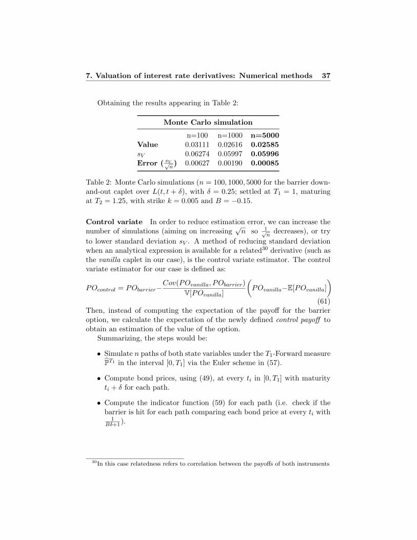
Obtaining the results appearing in Table 2:
Monte Carlo simulation
n=100 n=1000 n=5000Value 0.03111 0.02616 0.02585sV 0.06274 0.05997 0.05996Error ( sV√
n) 0.00627 0.00190 0.00085
Table 2: Monte Carlo simulations (n = 100, 1000, 5000 for the barrier down-and-out caplet over L(t, t + δ), with δ = 0.25; settled at T1 = 1, maturingat T2 = 1.25, with strike k = 0.005 and B = −0.15.
Control variate In order to reduce estimation error, we can increase thenumber of simulations (aiming on increasing
√n so 1√
ndecreases), or try
to lower standard deviation sV . A method of reducing standard deviationwhen an analytical expression is available for a related30 derivative (such asthe vanilla caplet in our case), is the control variate estimator. The controlvariate estimator for our case is defined as:
POcontrol = PObarrier−Cov(POvanilla, PObarrier)
V[POvanilla]
(POvanilla−E[POvanilla]
)(61)
Then, instead of computing the expectation of the payoff for the barrieroption, we calculate the expectation of the newly defined control payoff toobtain an estimation of the value of the option.
Summarizing, the steps would be:
• Simulate n paths of both state variables under the T1-Forward measurePT1 in the interval [0, T1] via the Euler scheme in (57).
• Compute bond prices, using (49), at every ti in [0, T1] with maturityti + δ for each path.
• Compute the indicator function (59) for each path (i.e. check if thebarrier is hit for each path comparing each bond price at every ti with
1Bδ+1).
30In this case relatedness refers to correlation between the payoffs of both instruments

7. Valuation of interest rate derivatives: Numerical methods 38
• Compute the payoff for both vanilla (using the last bond price of eachpath, that is P (T1, T1+δ) = P (T1, T2)) and barrier caplets (taking intoaccount the last bond price and the value of the indicator function foreach path).
• Define the control payoff as in (61), where E[POvanilla] can be analyti-cally computed using (58), but V[POvanilla] and Cov(POvanilla, PObarrier)have to be replaced with their sample counterparts.
• With n independent observations of the control payoff, calculate itssample mean and its sample standard deviation in order to obtain anestimation of the value of the barrier caplet and a measure of its error.
[Glasserman, 2003] points out that a ρ(POvanilla, PObarrier) around 0.7(the sample correlation coefficient between payoffs ρ(POvanilla, PObarrier) inour analysis is about 0.71) decreases the number of simulations required toobtain the same error to about half, with respect to the original case withoutcontrol variate. Following this idea, we try n = 2500 and check that thisis indeed the case, obtaining approximately the same error without controlvariate and n = 5000, than using control variate and setting n = 2500.These findings are summarized in Table 3.
Monte Carlo simulation(control variate)
n=100 n=1000 n=2500 n=5000Value 0.02778 0.02510 0.02546 0.02521sV 0.04749 0.04309 0.04245 0.04232Error ( sV√
n) 0.00475 0.00136 0.00084 0.00060
Table 3: Monte Carlo simulation results for the Barrier down-and-outcaplet over L(t, t + δ), with δ = 0.25; settled at T1 = 1, maturing atT2 = 1.25, with strike k = 0.005 and B = −0.15 with control variate forn = 100, 1000, 2500, 5000.
7.2 Numerical integration. European swaption
For the European swaption, we decide to use numerical integration to com-pute its value due to the path-independent nature of this derivative. Werecall the distribution of the state variables under PT1 at T1. As statedin Section 5, the two state variables are jointly normal, so they follow abivariate normal distribution.

7. Valuation of interest rate derivatives: Numerical methods 39
Considering:
X11(T1)PT1∼ N (0, a2T1)
d= a
√T1 N (0, 1)︸ ︷︷ ︸
x
X12(T1)PT1∼ N
(0,c2
2θ
[1− exp (−2θT1)
])d=
d=
c√2θ
√1− exp (−2θT1) N (0, 1)︸ ︷︷ ︸
y
we can work with the bivariate standard normal instead. The jointprobability density function under PT1 of X,Y is therefore:
f PT1
(x, y) =1
2πexp
[−1
2
(x2 + y2
)]The payoff for the European swaption (see (32)) in our model can be
expressed as a function of x and y, as
g(x, y) =
[K
(P (0, T2)
P (0, T1)exp
[− (T2 − T1)a
√T1x
− 1
θ
(1− exp[−θ(T2 − T1)]
)c√2θ
√1− exp (−2θT1)y
− 1
2(T2 − T1)2a2T1 −
1
2θ2
(1− exp [−θ(T2 − T1)]
)2 c2
2θ
[1− exp (−2θT1)
]]0.25
7. Valuation of interest rate derivatives: Numerical methods 40
+P (0, T3)
P (0, T1)exp
[− (T3 − T1)a
√T1x
− 1
θ
(1− exp[−θ(T3 − T1)]
)c√2θ
√1− exp (−2θT1)y
− 1
2(T3 − T1)2a2T1 −
1
2θ2
(1− exp [−θ(T3 − T1)]
)2 c2
2θ
[1− exp (−2θT1)
]]0.25
+P (0, T4)
P (0, T1)exp
[− (T4 − T1)a
√T1x
− 1
θ
(1− exp[−θ(T4 − T1)]
)c√2θ
√1− exp (−2θT1)y
− 1
2(T4 − T1)2a2T1 −
1
2θ2
(1− exp [−θ(T4 − T1)]
)2 c2
2θ
[1− exp (−2θT1)
]]0.25
+P (0, T5)
P (0, T1)exp
[− (T5 − T1)a
√T1x
− 1
θ
(1− exp[−θ(T5 − T1)]
)c√2θ
√1− exp (−2θT1)y
− 1
2(T5 − T1)2a2T1 −
1
2θ2
(1− exp [−θ(T5 − T1)]
)2 c2
2θ
[1− exp (−2θT1)
]]0.25
)
+P (0, T5)
P (0, T1)exp
[− (T5 − T1)a
√T1x
− 1
θ
(1− exp[−θ(T5 − T1)]
)c√2θ
√1− exp (−2θT1)y
− 1
2(T5 − T1)2a2T1 −
1
2θ2
(1− exp [−θ(T5 − T1)]
)2 c2
2θ
[1− exp (−2θT1)
]]− 1
]+
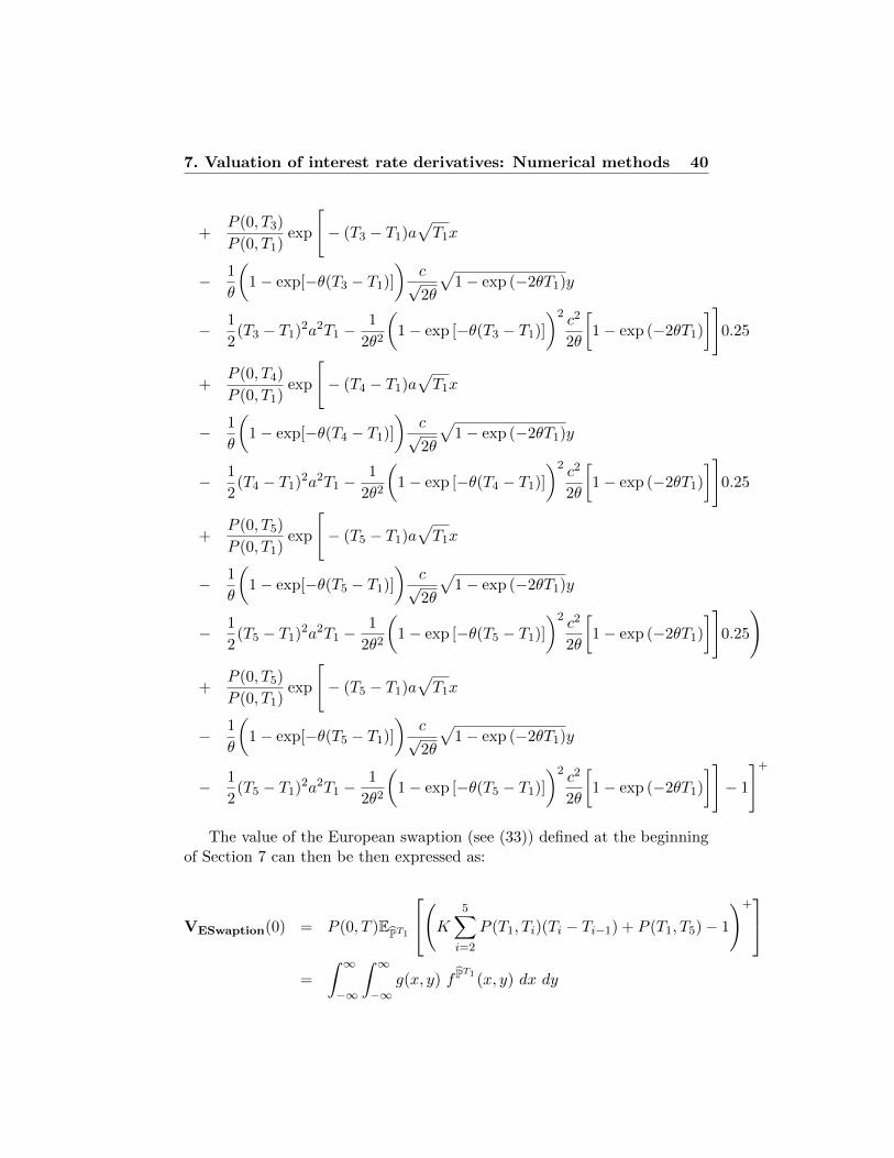
The value of the European swaption (see (33)) defined at the beginningof Section 7 can then be then expressed as:
VESwaption(0) = P (0, T )EPT1
(K 5∑i=2
P (T1, Ti)(Ti − Ti−1) + P (T1, T5)− 1
)+
=
∫ ∞−∞
∫ ∞−∞
g(x, y) f PT1
(x, y) dx dy
7. Valuation of interest rate derivatives: Numerical methods 41
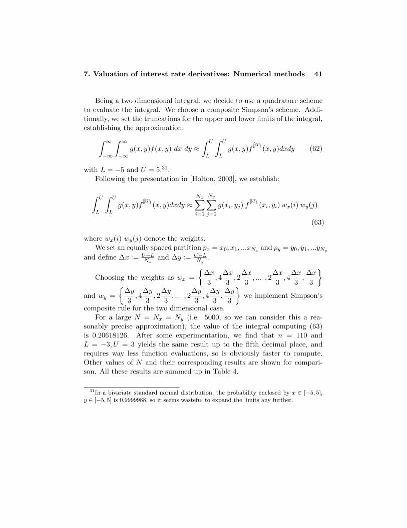
Being a two dimensional integral, we decide to use a quadrature schemeto evaluate the integral. We choose a composite Simpson’s scheme. Addi-tionally, we set the truncations for the upper and lower limits of the integral,establishing the approximation:∫ ∞
−∞
∫ ∞−∞
g(x, y)f(x, y) dx dy ≈∫ U
L
∫ U
Lg(x, y)f P
T1(x, y)dxdy (62)
with L = −5 and U = 5.31.Following the presentation in [Holton, 2003], we establish:
∫ U
L
∫ U
Lg(x, y)f P
T1(x, y)dxdy ≈
Nx∑i=0
Ny∑j=0
g(xi, yj) fPT1 (xi, yi) wx(i) wy(j)
(63)
where wx(i) wy(j) denote the weights.We set an equally spaced partition px = x0, x1, ...xNx and py = y0, y1, ...yNy
and define ∆x := U−LNx
and ∆y := U−LNy
.
Choosing the weights as wx =
{∆x
3, 4
∆x
3, 2
∆x
3, ... , 2
∆x
3, 4
∆x
3,∆x
3
}and wy =
{∆y
3, 4
∆y
3, 2
∆y
3, ... , 2
∆y
3, 4
∆y
3,∆y
3
}we implement Simpson’s
composite rule for the two dimensional case.For a large N = Nx = Ny (i.e. 5000, so we can consider this a rea-
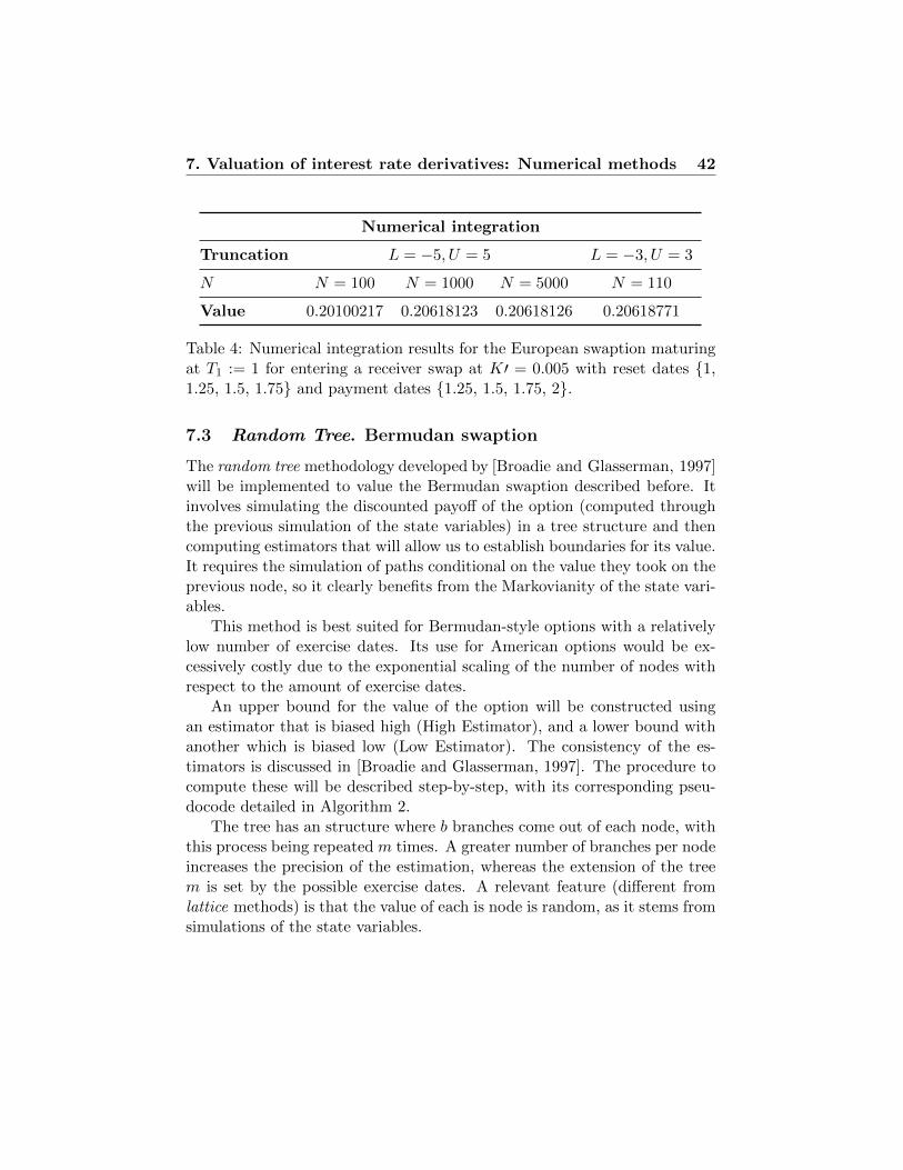
sonably precise approximation), the value of the integral computing (63)is 0.20618126. After some experimentation, we find that n = 110 andL = −3, U = 3 yields the same result up to the fifth decimal place, andrequires way less function evaluations, so is obviously faster to compute.Other values of N and their corresponding results are shown for compari-son. All these results are summed up in Table 4.
31In a bivariate standard normal distribution, the probability enclosed by x ∈ [−5, 5],y ∈ [−5, 5] is 0.9999988, so it seems wasteful to expand the limits any further.
7. Valuation of interest rate derivatives: Numerical methods 42
Numerical integration
Truncation L = −5, U = 5 L = −3, U = 3
N N = 100 N = 1000 N = 5000 N = 110
Value 0.20100217 0.20618123 0.20618126 0.20618771
Table 4: Numerical integration results for the European swaption maturingat T1 := 1 for entering a receiver swap at K′ = 0.005 with reset dates {1,1.25, 1.5, 1.75} and payment dates {1.25, 1.5, 1.75, 2}.
7.3 Random Tree. Bermudan swaption
The random tree methodology developed by [Broadie and Glasserman, 1997]will be implemented to value the Bermudan swaption described before. Itinvolves simulating the discounted payoff of the option (computed throughthe previous simulation of the state variables) in a tree structure and thencomputing estimators that will allow us to establish boundaries for its value.It requires the simulation of paths conditional on the value they took on theprevious node, so it clearly benefits from the Markovianity of the state vari-ables.
This method is best suited for Bermudan-style options with a relativelylow number of exercise dates. Its use for American options would be ex-cessively costly due to the exponential scaling of the number of nodes withrespect to the amount of exercise dates.
An upper bound for the value of the option will be constructed usingan estimator that is biased high (High Estimator), and a lower bound withanother which is biased low (Low Estimator). The consistency of the es-timators is discussed in [Broadie and Glasserman, 1997]. The procedure tocompute these will be described step-by-step, with its corresponding pseu-docode detailed in Algorithm 2.
The tree has an structure where b branches come out of each node, withthis process being repeated m times. A greater number of branches per nodeincreases the precision of the estimation, whereas the extension of the treem is set by the possible exercise dates. A relevant feature (different fromlattice methods) is that the value of each is node is random, as it stems fromsimulations of the state variables.

7. Valuation of interest rate derivatives: Numerical methods 43
We provide a graphical representation of a tree with m = 2, b = 2, toclarify the idea.
Figure 2: Example of one simulation of the tree structure for a given under-lying process, with m = 2, b = 2 and time step of 1. After the initial nodeat t = 0, we have b nodes at t = 1 and b2 nodes at t = 2.
Now we will explain the tree construction procedure for our model andthe computation of the High and Low estimators for the value of the Bermu-dan swaption.
Trees for the state variables The tree structure for the state variablesis built as follows: for each node before the terminal ones, simulate b inde-pendent replications of the trajectory of the state variable up to the nextnode using (57), conditional on the value of the starting node. Then repeatthe process for the second state variable.
7. Valuation of interest rate derivatives: Numerical methods 44
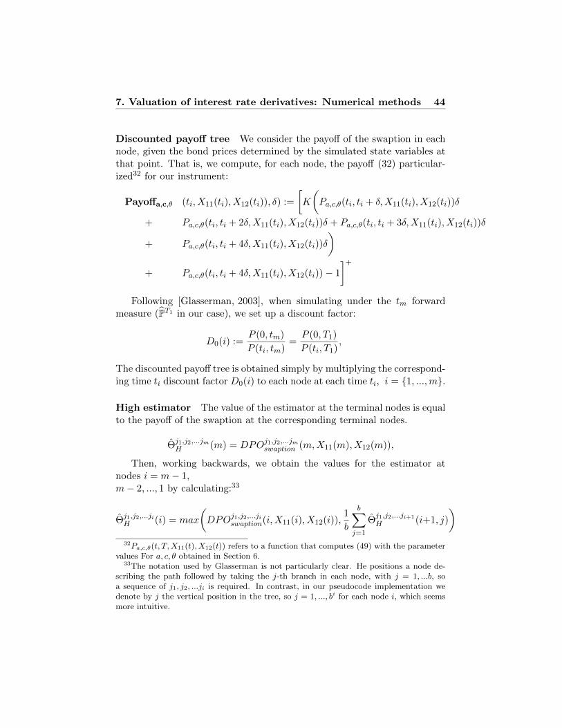
Discounted payoff tree We consider the payoff of the swaption in eachnode, given the bond prices determined by the simulated state variables atthat point. That is, we compute, for each node, the payoff (32) particular-ized32 for our instrument:
Payoffa,c,θ (ti, X11(ti), X12(ti)), δ) :=
[K
(Pa,c,θ(ti, ti + δ,X11(ti), X12(ti))δ
+ Pa,c,θ(ti, ti + 2δ,X11(ti), X12(ti))δ + Pa,c,θ(ti, ti + 3δ,X11(ti), X12(ti))δ
+ Pa,c,θ(ti, ti + 4δ,X11(ti), X12(ti))δ
)+ Pa,c,θ(ti, ti + 4δ,X11(ti), X12(ti))− 1
]+
Following [Glasserman, 2003], when simulating under the tm forwardmeasure (PT1 in our case), we set up a discount factor:
D0(i) :=P (0, tm)
P (ti, tm)=P (0, T1)
P (ti, T1),
The discounted payoff tree is obtained simply by multiplying the correspond-ing time ti discount factor D0(i) to each node at each time ti, i = {1, ...,m}.
High estimator The value of the estimator at the terminal nodes is equalto the payoff of the swaption at the corresponding terminal nodes.
Θj1,j2,...jmH (m) = DPOj1,j2,...jmswaption (m,X11(m), X12(m)),
Then, working backwards, we obtain the values for the estimator atnodes i = m− 1,m− 2, ..., 1 by calculating:33
Θj1,j2,...jiH (i) = max
(DPOj1,j2,...jiswaption(i,X11(i), X12(i)),
1
b
b∑j=1
Θj1,j2,...ji+1
H (i+1, j)
)32Pa,c,θ(t, T,X11(t), X12(t)) refers to a function that computes (49) with the parameter
values For a, c, θ obtained in Section 6.33The notation used by Glasserman is not particularly clear. He positions a node de-
scribing the path followed by taking the j-th branch in each node, with j = 1, ...b, soa sequence of j1, j2, ...ji is required. In contrast, in our pseudocode implementation wedenote by j the vertical position in the tree, so j = 1, ..., bi for each node i, which seemsmore intuitive.
7. Valuation of interest rate derivatives: Numerical methods 45
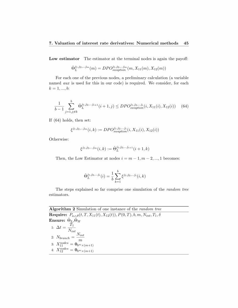
Low estimator The estimator at the terminal nodes is again the payoff:
Θj1,j2,...jmL (m) = DPOj1,j2,...jmswaption (m,X11(m), X12(m))
For each one of the previous nodes, a preliminary calculation (a variablenamed aux is used for this in our code) is required. We consider, for eachk = 1, ..., b:
1
b− 1
b∑j=1,j 6=k
Θj1,j2,...ji+1
L (i+ 1, j) ≤ DPOj1,j2,...jiswaption(i,X11(i), X12(i)) (64)
If (64) holds, then set:
ξj1,j2,...jm(i, k) := DPOj1,j2,...jiswaption(i,X11(i), X12(i))
Otherwise:
ξj1,j2,...jm(i, k) := Θj1,j2,...ji+1
L (i+ 1, k)
Then, the Low Estimator at nodes i = m− 1,m− 2, ..., 1 becomes:
Θj1,j2,...jiL (i) =
1
b
b∑k=1
ξj1,j2,...ji(i, k)
The steps explained so far comprise one simulation of the random treeestimators.
Algorithm 2 Simulation of one instance of the random tree
Require: Pa,c,θ(t, T,X11(t), X12(t)), P (0, T ), b,m,Nint, T1, δ
Ensure: ΘL,ΘH
1: ∆t =T1
Nint
2: Nbranch =Nint
m3: Xnodes
11 = 0bm×(m+1)
4: Xnodes12 = 0bm×(m+1)

7. Valuation of interest rate derivatives: Numerical methods 46
. Trees for the state variables5: for i = 2 to m+ 1 do6: for j = 1 to b(i−1) do
7: counter =
⌈j
b
⌉8: Xsimul
11 [1] = Xnodes11 [counter, i− 1]
9: Xsimul12 [1] = Xnodes
12 [counter, i− 1]10: for k = 1 to Nbranch − 1 do
11: Xsimul11 [k+ 1] = Xsimul
11 [k] +a2
(2(Nbranch(i− 2) +k)−T1
)∆t
12: + a√
∆t randomN (0,1)
13: Xsimul12 [k + 1] = Xsimul
12 [k] +
(− θXsimul
12 [k] +c2
2θ
(1
14: − exp(−2θ∆t(Nbranch ∗ (i− 2) + k))
)15: +
c2
θ
(exp(−θ(T1−∆t(Nbranch∗(i−2)+k)))−1
))∆t
16: + c√
∆t randomN (0,1)
17: end for k18: Xnodes
11 [j, i] = Xsimul11 [Nbranch]
19: Xnodes12 [j, i] = Xsimul
12 [Nbranch]20: end for j21: end for i22: POnodesswaption = 0bm×m+1
. Discounted payoff tree23: for i = 1 to m+ 1 do24: for j = 1 to b(i−1) do
25: counter =
⌈j
b
⌉26: POnodesswaption[j, i] = Payoffa,c,θ(∆t Nbranch(i− 1),
27: , Xnodes11 [j, i], Xnodes
12 [j, i], δ)28: end for j29: end for i30: PT1−mat = 0bm×m+1 ; PT1−mat[1, 1] = Pa,c,θ[0, T1, 0, 0]31: for i = 2 to m+ 1 do32: for j = 1 to b(i−1) do
33: counter =
⌈j
b
⌉34: PT1−mat[j, i] = Pa,c,θ(∆tNbranch(i−1), T1, X
nodes11 [j, i], Xnodes
12 [j, i])35: end for j36: end for i

7. Valuation of interest rate derivatives: Numerical methods 47
37: DPOnodesswaption = 0bm×m+1 ; DPOnodesswaption[1, 1] = POnodesswaption[1, 1]38: for i = 2 to m+ 1 do39: for j = 1 to b(i−1) do
40: counter =
⌈j
b
⌉41: disc =
Pa,c,θ(0, T1, 0, 0)
PT1−mat[j, i]42: DPOnodesswaption[j, i] = discPOnodesswaption[j, i]43: end for j44: end for i
. High Estimator45: HEnodes = 0bm×m+1 ; HEnodes[ : ,m+ 1] = DPOnodesswaption[ : ,m+ 1]46: for i = (m+ 1)− 1 to 1 step −1 do47: for j = 1 to b(i−1) do
48: HEnodes[j, i] = max(DPO[j, i],1
bΣ(HE[jb− (b− 1) : jb, i+ 1]]))
49: end for j50: end for i51: ΘH = HEnodes[1, 1]
. Low Estimator52: LEnodes = 0bm×m+1 ; LEnodes[ : ,m+ 1] = DPOnodesswaption[ : ,m+ 1]53: for i = (m+ 1)− 1 to 1 step −1 do54: for j = 1 to b(i−1) do55: for k = 1 to b do56: aux = 0k×1
57: if DPOnodesswaption[j, i] >1
b− 1
(Σ(HE[jb− (b− 1) : jb, i+ 1])
58: −HE[j ∗ b+k− b, i+ 1]
)then
59: aux [k] = DPOnodesswaption[j, i]60: else61: aux [k] = LEnodes[j + k − 1, i+ 1]62: end if
63: LEnodes[j, i] =1
bΣ(aux)
64: end for k65: end for j66: end for i67: ΘL = LEnodes[1, 1]68: return ΘL,ΘH

7. Valuation of interest rate derivatives: Numerical methods 48
Confidence interval for the value of the Bermudan swaption Theconfidence interval defined in [Broadie and Glasserman, 1997] sets the upperbound as: 34
1
n
n∑i=1
ΘH,{i} +Φ(η2 )sΘH√
n
And the lower bound:
1
n
n∑i=1
ΘL,{i} −Φ(η2 )sΘL√
n
Repeating the process n times to obtain n independent replications andcomputing the sample mean and sample standard deviation of {ΘL(1), ΘL(2),
... , ΘL(n)} and {ΘH(1), ΘH(2), ... , ΘH(n)}, we can obtain a confidenceinterval for VBSwaption(0).
In Table 5 we show the upper and lower bounds that define the confidenceintervals for η = 0.05, with n = 500 simulations of the tree, and b = 2, 3, 4, 5.
Parameter b
2 3 4 5
1500
∑500i=1 ΘL,{i} 0.2418 0.2673 0.2615 0.2625
1500
∑500i=1 ΘH,{i} 0.3252 0.3018 0.2818 0.2744
sΘL0.2726 0.2800 0.2791 0.2840
sΘH0.2679 0.1869 0.1422 0.1248
Lower bound 0.2316 0.2569 0.2511 0.2519Upper bound 0.3352 0.3088 0.2871 0.2791
Table 5: Random tree simulations (n = 500) for the Bermudan swaptionwith different values of b = 2, 3, 4, 5.
34The notation ΘH,{i} refers to the value of the High Estimator in simulation i.

8. Concluding remarks 49
8 Concluding remarks
Some of the limitations and possible extensions of the work done so far areoutlined:
• Calibration could have been made to a broader set of instruments.During the process it was seen that many different combinations ofparameters were able to approximately reproduce the market price ofcaplets for the particular strike chosen, indicating that there is stillroom within the model for considering further market data.
• A great deal of bond price volatility is present in our simulations,that could indicate that other values of the parameters, yet to befound, might be more adequate. To that regard, additional optimiza-tion methods, such as the Nelder-Mead algorithm, could have beentested.
• The multicurve approach to valuation of interest rate derivatives wasnot considered in order to simplify the exposition, and it is certainlyan extension that should be included.
• Instantaneous correlation between the two Brownian motions drivingthe model could be introduced to allow for grater flexibility. More dra-matic extensions such as stochastic volatility would require a completerework of the exposition.
• A PDE formulation of the valuation of the instruments could have beenintroduced using Feynman-Kac (as in [Valero et al., 2011] or [Beyna, 2013]),making further use of the Markovianity of the state variables.
• As noted during the work, the β(t) function in (35) can be freelychosen (although being easily differentiable and integrable is highlyrecommended) without adding any state variables, so a more complexfunction could be chosen in order the improve the capabilities of themodel, at the expense of lengthier computations.

A. Computations in the Two-Factor Cheyette model 50
A Computations in the Two-Factor Cheyette model
A.1 Instantaneous forward rate
In our Two-Factor model, we have M = 2, N1 = 1 and N2 = 1, so insertingthe Cheyette volatility (35) in the integrated two factor version of (23) weget:
f(t, T ) = f(0, T ) +
∫ t
0
(α11(T )
α11(s)β11(s)
[∫ T
s
α11(u)
α11(s)β11(s)du
])ds
+
∫ t
0
(α12(T )
α12(s)β12(s)
[∫ T
s
α12(u)
α12(s)β12(s)du
])ds
+
∫ t
0
(α11(T )
α11(s)β11(s)
)dW1(s) +
∫ t
0
(α12(T )
α12(s)β12(s)
)dW2(s)
Pulling terms out of the Riemann integrals:
= f(0, T ) +
∫ t
0
(α11(T )
α11(s)β11(s)
[β11(s)
α11(s)
∫ T
sα11(u)du+
])ds
+
∫ t
0
(α12(T )
α12(s)β12(s)
[β12(s)
α12(s)
∫ T
sα12(u)du
])ds
+
∫ t
0
(α11(T )
α11(s)β11(s)
)dW1(s) +
∫ t
0
(α12(T )
α12(s)β12(s)
)dW2(s)
= f(0, T ) +
∫ t
0
(α11(T )β11(s)β11(s)
α11(s)α11(s)
∫ T
sα11(u)du
)ds
+
∫ t
0
(α12(T )β12(s)β12(s)
α12(s)α12(s)
∫ T
sα12(u)du
)ds
+
∫ t
0
(α11(T )
α11(s)β11(s)
)dW1(s) +
∫ t
0
(α12(T )
α12(s)β12(s)
)dW2(s)

A. Computations in the Two-Factor Cheyette model 51
Multiplying the integrals byα1i(t)
α1i(t), noting that
∫ Ts α1i(u)du = A1i(T )−
A1i(s), and adding ±A1i(t) inside the Riemann integrals:
= f(0, T ) +
∫ t
0
(α11(T )β11(s)β11(s)
α11(s)α11(s)[A11(T )−A11(s)]
+α12(T )β12(s)β12(s)
α12(s)α12(s)[A12(T )−A12(s)]
)ds
+α11(T )
α11(t)
∫ t
0
α11(t)
α11(s)β11(s)dW1(s) +
α12(T )
α12(t)
∫ t
0
α12(t)
α12(s)β12(s)dW2(s)
= f(0, T ) +
∫ t
0
(α11(t)
α11(t)
α11(T )β11(s)β11(s)
α11(s)α11(s)[A11(t)−A11(s)]
+α12(t)
α12(t)
α12(T )β12(s)β12(s)
α12(s)α12(s)[A12(t)−A12(s)]
)ds
+
∫ t
0
(α11(t)
α11(t)
α11(T )β11(s)β11(s)
α11(t)α11(s)[A11(T )−A11(t)]
+α12(t)
α12(t)
α12(T )β12(s)β12(s)
α12(s)α12(s)[A12(T )−A12(t)]
)ds
+α11(T )
α11(t)
∫ t
0
α11(t)
α11(s)β11(s)dW1(s) +
α12(T )
α12(t)
∫ t
0
α12(t)
α12(s)β12(s)dW2(s)
= f(0, T ) +α11(T )
α11(t)
∫ t
0
(α11(t)β11(s)β11(s)
α11(s)α11(s)[A11(t)−A11(s)]
)ds
+α12(T )
α12(t)
∫ t
0
(α12(t)β12(s)β12(s)
α12(s)α12(s)[A12(t)−A12(s)]
)ds
+
∫ t
0
(α11(t)
α11(t)
α11(T )β11(s)β11(s)
α11(s)α11(s)[A11(T )−A11(t)]
)ds
+
∫ t
0
(α12(t)
α12(t)
α12(T )β12(s)β12(s)
α12(s)α12(s)[A12(T )−A12(t)]
)ds
+α11(T )
α11(t)
∫ t
0
α11(t)
α11(s)β11(s)dW1(s) +
α12(T )
α12(t)
∫ t
0
α12(t)
α12(s)β12(s)dW2(s)

A. Computations in the Two-Factor Cheyette model 52
Rearranging and pulling elements out of the integrals:
= f(0, T ) +α11(T )
α11(t)
∫ t
0
(α11(t)β11(s)
α11(s)
[A11(t)−A11(s)]
α11(s)β11(s)
)ds
+α12(T )
α12(t)
∫ t
0
(α12(t)β12(s)
α12(s)
[A12(t)−A12(s)]
α12(s)β12(s)
)ds
+α11(T )[A11(T )−A11(t)]
α11(t)α11(t)
∫ t
0
(α11(t)α11(t)
α11(s)α11(s)β11(s)β11(s)
)ds
+α12(T )[A12(T )−A12(t)]
α12(t)α12(t)
∫ t
0
(α12(t)α12(t)
α12(s)α12(s)β12(s)β12(s)
)ds
+α11(T )
α11(t)
∫ t
0
α11(t)
α11(s)β11(s)dW1(s) +
α12(T )
α12(t)
∫ t
0
α12(t)
α12(s)β12(s)dW2(s)
= f(0, T ) +α11(T )
α11(t)
∫ t
0
(α11(t)β11(s)
α11(s)
[A11(t)−A11(s)]
α11(s)β11(s))ds
+α12(T )
α12(t)
∫ t
0
(α12(t)β12(s)
α12(s)
[A12(t)−A12(s)]
α12(s)β12(s)
)ds
+α11(T )
α11(t)
[A11(T )−A11(t)]
α11(t)
∫ t
0
(α11(t)α11(t)
α11(s)α11(s)β11(s)β11(s)
)ds
+α12(T )
α12(t)
[A12(T )−A12(t)]
α12(t)
∫ t
0
(α12(t)α12(t)
α12(s)α12(s)β12(s)β12(s)
)ds
+α11(T )
α11(t)
∫ t
0
α11(t)
α11(s)β11(s)dW1(s) +
α12(T )
α12(t)
∫ t
0
α12(t)
α12(s)β12(s)dW2(s)
Taking into account the definitions of Aij(t) and Vij,k(t) stated in (36)and (37) respectively, and also collecting terms:
= f(0, T ) +α11(T )
α11(t)
[∫ t
0
(α11(t)β11(s)
α11(s)
[A11(t)−A11(s)]
α11(s)β11(s)
)ds
+[A11(T )−A11(t)]
α11(t)V11,1(t) +
∫ t
0
α11(t)
α11(s)β11(s)dW1(s)
]+
α12(T )
α12(t)
[∫ t
0
(α12(t)β12(s)
α12(s)
[A12(t)−A12(s)]
α12(s)β12(s)
)ds
+[A12(T )−A12(t)]
α12(t)V11,2(t) +
∫ t
0
α12(t)
α12(s)β12(s)dW2(s)
]

A. Computations in the Two-Factor Cheyette model 53
Applying the definition for the state variable, Xjk(t), in (38):
= f(0, T ) +α11(T )
α11(t)
[X11(t) +
[A11(T )−A11(t)]
α11(t)V11,1(t)
]+
α12(T )
α12(t)
[X12(t) +
[A12(T )−A12(t)]
α12(t)V11,2(t)
]Collecting terms in summations we arrive to the following expression, withk = 1, 2 and N1 = 1, N2 = 1:
f(t, T ) = f(0, T ) +2∑
k=1
[α1k(T )
α1k(t)
[X1k(t) +
[A1k(T )−A1k(t)]
α1k(t)V11,k(t)
]](65)
which is easily related to the general case expression of (40).

A. Computations in the Two-Factor Cheyette model 54
A.2 Zero-coupon bond price
Using the expression for the zero-coupon bond in terms of the instantaneousforward rate (6), and (65) we have:
P (t, T ) = exp
(−∫ T
tf(t, u)du
)= exp
(−∫ T
tf(0, u) +
α11(u)
α11(t)
[X11(t) +
[A11(u)−A11(t)]
α11(t)V11,1(t)
]+
α12(u)
α12(t)
[X12(t) +
[A12(u)−A12(t)]
α12(t)V11,2(t)
]du
)=
P (0, T )
P (0, t)exp
(−∫ T
t
(α11(u)
α11(t)X11(t) +
α12(u)
α12(t)X12(t)
)du
−∫ T
t
(α11(u)
α11(t)
[A11(u)−A11(t)]
α11(t)V11,1(t) +
α12(u)
α12(t)
[A12(u)−A12(t)]
α12(t)V11,2(t)
)du
)Recalling that by the definition ofAij(t) we haveA1j(u)−A1j(t) =
∫ ut α1j(s)ds,
and extracting terms out of the integrals:
=P (0, T )
P (0, t)exp
(−∫ T
t
(α11(u)
α11(t)X11(t) +
α12(u)
α12(t)X12(t)
)du
−∫ T
t
(α11(u)
α11(t)
(∫ u
t
α11(s)
α11(t)ds
)V11,1(t) +
α12(u)
α12(t)
(∫ u
t
α12(s)
α12(t)ds
)V11,2(t)
)du
)=
P (0, T )
P (0, t)exp
(−∫ T
t
α11(u)
α11(t)X11(t)du−
∫ T
t
α12(u)
α12(t)X12(t)du
− 1
α11(t)α11(t)V11,1(t)
∫ T
tα11(u)[A11(u)−A11(t)]du
− 1
α12(t)α12(t)V11,2(t)
∫ T
tα12(u)[A12(u)−A12(t)]du
)

A. Computations in the Two-Factor Cheyette model 55
Computing the integrals we arrive at:
=P (0, T )
P (0, t)exp
(− X11(t)
α11(t)
∫ T
tα11(u)du− X12(t)
α12(t)
∫ T
tα12(u)du
− (A11(T )−A11(t))2
2α11(t)α11(t)V11,1(t)− (A12(T )−A12(t))2
2α12(t)α12(t)V11,2(t)
)=
P (0, T )
P (0, t)exp
(− A11(T )−A11(t)
α11(t)X11(t)− A12(T )−A12(t)
α12(t)X12(t)
− (A11(T )−A11(t))2
2α11(t)α11(t)V11,1(t)− (A12(T )−A12(t))2
2α12(t)α12(t)V11,2(t)
)
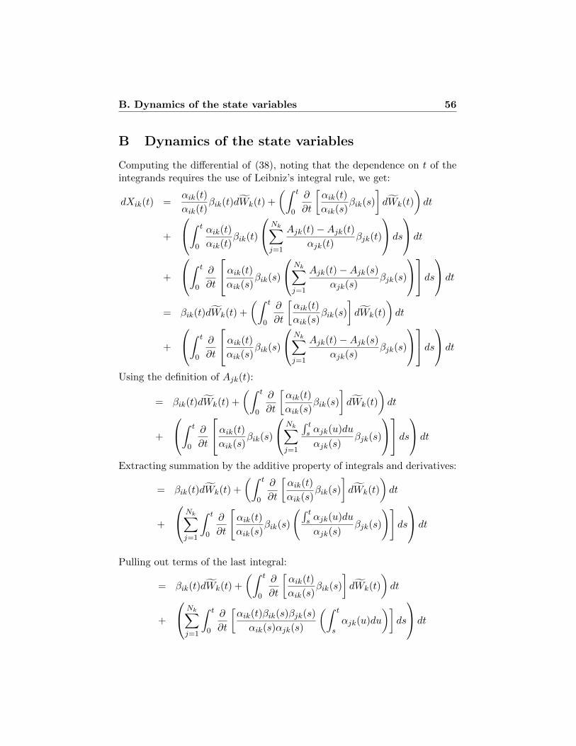
B. Dynamics of the state variables 56
B Dynamics of the state variables
Computing the differential of (38), noting that the dependence on t of theintegrands requires the use of Leibniz’s integral rule, we get:
dXik(t) =αik(t)
αik(t)βik(t)dWk(t) +
(∫ t
0
∂
∂t
[αik(t)
αik(s)βik(s)
]dWk(t)
)dt
+
∫ t
0
αik(t)
αik(t)βik(t)
Nk∑j=1
Ajk(t)−Ajk(t)αjk(t)
βjk(t)
ds
dt
+
∫ t
0
∂
∂t
αik(t)αik(s)
βik(s)
Nk∑j=1
Ajk(t)−Ajk(s)αjk(s)
βjk(s)
ds dt
= βik(t)dWk(t) +
(∫ t
0
∂
∂t
[αik(t)
αik(s)βik(s)
]dWk(t)
)dt
+
∫ t
0
∂
∂t
αik(t)αik(s)
βik(s)
Nk∑j=1
Ajk(t)−Ajk(s)αjk(s)
βjk(s)
ds dt
Using the definition of Ajk(t):
= βik(t)dWk(t) +
(∫ t
0
∂
∂t
[αik(t)
αik(s)βik(s)
]dWk(t)
)dt
+
∫ t
0
∂
∂t
αik(t)αik(s)
βik(s)
Nk∑j=1
∫ ts αjk(u)du
αjk(s)βjk(s)
ds dt
Extracting summation by the additive property of integrals and derivatives:
= βik(t)dWk(t) +
(∫ t
0
∂
∂t
[αik(t)
αik(s)βik(s)
]dWk(t)
)dt
+
Nk∑j=1
∫ t
0
∂
∂t
[αik(t)
αik(s)βik(s)
(∫ ts αjk(u)du
αjk(s)βjk(s)
)]ds
dt
Pulling out terms of the last integral:
= βik(t)dWk(t) +
(∫ t
0
∂
∂t
[αik(t)
αik(s)βik(s)
]dWk(t)
)dt
+
Nk∑j=1
∫ t
0
∂
∂t
[αik(t)βik(s)βjk(s)
αik(s)αjk(s)
(∫ t
sαjk(u)du
)]ds
dt

B. Dynamics of the state variables 57
Extracting terms out of the derivative:
= βik(t)dWk(t) +
(∫ t
0
∂
∂t
[αik(t)
αik(s)βik(s)
]dWk(t)
)dt
+
Nk∑j=1
∫ t
0
βik(s)βjk(s)
αik(s)αjk(s)
∂
∂t
[αik(t)
(∫ t
sαjk(u)du
)]ds
dt
Computing the derivative in the second summand using the product rule:
= βik(t)dWk(t) +
(∫ t
0
∂
∂t
[αik(t)
αik(s)βik(s)
]dWk(t)
)dt
+
Nk∑j=1
∫ t
0
βik(s)βjk(s)
αik(s)αjk(s)
[∂αik(t)
∂t
∫ t
sαjk(u)du+ αik(t)αjk(t)
]ds
dt
= βik(t)dWk(t) +
(∫ t
0
∂
∂t
[αik(t)
αik(s)βik(s)
]dWk(t)
)dt
+
(Nk∑j=1
(∫ t
0
βik(s)βjk(s)
αik(s)αjk(s)
∂αik(t)
∂t
(∫ t
sαjk(u)du
)ds
+
∫ t
0
βik(s)βjk(s)
αik(s)αjk(s)αik(t)αjk(t)ds
))dt
Rearranging derivatives and integrals:
= βik(t)dWk(t) +
(∫ t
0
∂
∂t
[αik(t)
αik(s)βik(s)
]dWk(t)
)dt
+
(Nk∑j=1
(∂αik(t)
∂t
∫ t
0
∫ t
s
βik(s)βjk(s)
αik(s)αjk(s)αjk(u)duds+ αik(t)αjk(t)
∫ t
0
βik(s)βjk(s)
αik(s)αjk(s)ds
))dt
= βik(t)dWk(t) +
(∫ t
0
∂
∂t
[αik(t)
αik(s)βik(s)
]dWk(t)
)dt
+
Nk∑j=1
(∂αik(t)
∂t
∫ t
0
βik(s)βjk(s)
αik(s)αjk(s)
∫ t
sαjk(u)duds+ αik(t)αjk(t)
∫ t
0
βik(s)βjk(s)
αik(s)αjk(s)ds
) dt
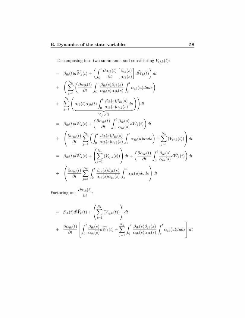
B. Dynamics of the state variables 58
Decomposing into two summands and substituting Vij,k(t):
= βik(t)dWk(t) +
(∫ t
0
∂αik(t)
∂t
[βik(s)
αik(s)
]dWk(t)
)dt
+
(Nk∑j=1
(∂αik(t)
∂t
∫ t
0
βik(s)βjk(s)
αik(s)αjk(s)
∫ t
sαjk(u)duds
)
+
Nk∑j=1
(αik(t)αjk(t)
∫ t
0
βik(s)βjk(s)
αik(s)αjk(s)ds︸ ︷︷ ︸
Vij,k(t)
))dt
= βik(t)dWk(t) +
(∂αik(t)
∂t
∫ t
0
βik(s)
αik(s)dWk(t)
)dt
+
∂αik(t)∂t
Nk∑j=1
(∫ t
0
βik(s)βjk(s)
αik(s)αjk(s)
∫ t
sαjk(u)duds
)+
Nk∑j=1
(Vij,k(t))
dt
= βik(t)dWk(t) +
Nk∑j=1
(Vij,k(t))
dt+
(∂αik(t)
∂t
∫ t
0
βik(s)
αik(s)dWk(t)
)dt
+
∂αik(t)∂t
Nk∑j=1
∫ t
0
βik(s)βjk(s)
αik(s)αjk(s)
∫ t
sαjk(u)duds
dt
Factoring out∂αik(t)
∂t:
= βik(t)dWk(t) +
Nk∑j=1
(Vij,k(t))
dt
+∂αik(t)
∂t
∫ t
0
βik(s)
αik(s)dWk(t) +
Nk∑j=1
∫ t
0
βik(s)βjk(s)
αik(s)αjk(s)
∫ t
sαjk(u)duds
dt

B. Dynamics of the state variables 59
Switching summation and intergal, computing the inner integral, andextracting i terms from the j-indexed summation we get:
= βik(t)dWk(t) +
Nk∑j=1
(Vij,k(t))
dt
+∂αik(t)
∂t
∫ t
0
βik(s)
αik(s)dWk(t) +
∫ t
0
βik(s)
αik(s)
Nk∑j=1
βjk(s)
αjk(s)[Ajk(t)−Ajk(s)]ds
dt
Noting that∂logαik(t)
∂t=
∂αik(t)
∂tαik(t)
, then∂αik(t)
∂t= αik(t)
∂logαik(t)
∂tand therefore:
= βik(t)dWk(t) +
Nk∑j=1
(Vij,k(t))
dt
+ αik(t)∂logαik(t)
∂t
∫ t
0
βik(s)
αik(s)dWk(t) +
∫ t
0
βik(s)
αik(s)
Nk∑j=1
[Ajk(t)−Ajk(s)]αjk(s)
βjk(s)ds
dtUsing the definition of Xik(t):
= βik(t)dWk(t) +
Nk∑j=1
(Vij,k(t))
dt
+∂logαik(t)
∂t
∫ t
0
αik(t)βik(s)
αik(s)dWk(t) +
∫ t
0
αik(t)βik(s)
αik(s)
Nk∑j=1
[Ajk(t)−Ajk(s)]αjk(s)
βjk(s)ds︸ ︷︷ ︸Xik(t)
dt
Finally, grouping dt terms we obtain the expression in (39):
dXik(t) = βik(t)dWk(t) +
Nk∑j=1
(Vij,k(t))
dt+∂logαik(t)
∂t[Xik(t)] dt
= βik(t)dWk(t) +
Nk∑j=1
(Vij,k(t)) +∂logαik(t)
∂tXik(t)
dt
C. Cubic spline yield-curve interpolation and caplet stripping 60
C Cubic spline yield-curve interpolation and capletstripping
Dataset
The dataset used comprises OIS zero rates as seen at a particular date(3/21/2019) with maturities TOIS ∈ { 1
12 ,212 , ... , 1, 2, ... , 10, 12, 15, 20, 25, 30},
and EUR caps with maturities Tcaps ∈ {1, 1.5, 2, ... , 10, 12, 15, 20, 25, 30}.The settle dates for these are trimonthly until year 2, becoming semiannualafter. Also, the very first caplet (which has no randomness attached toit) is not considered, so the relevant dates for caplets become Tsettle,caplets ∈{0.25, 0.5, 0.75, 1, 1.25, ... , 28, 28.5, 29, 29.5} and Tmaturity,caplets ∈ {0.5, 0.75, 1,1.25, ... , 28, 28.5, 29, 29.5, 30}. Market quotes for caps are not prices but im-plied normal35 flat volatilities, in order to retrieve cap prices we would needto plug them in Bachelier formula for caps. Even further, it would be prefer-able to work with caplets, the fundamental pieces, instead of caps, so we willtry to deduce them in a process called stripping.
Cubic spline interpolation
In order to perform caplet stripping, we require discount factors not onlyat dates quoted in the market, but at every relevant caplet date: interpola-tion is therefore required. Cubic spline obtains a smooth function (a set offunctions pasted together) that, by construction, includes all the data pointssupplied. The property of exactly recovering original data is the main reasonfor its use.
Considering a data set of n + 1 elements, a spline S(x) is a piecewisefunction, whose n pieces are third order polynomials, so for i = 1, ..., n wehave:
S(x) =
S1(x) = a1(x− x1)3 + b1(x− x1)2 + c1(x− x1) + d1 If x0 ≤ x ≤ x1,
...Si(x) = ai(x− xi)3 + bi(x− xi)2 + ci(x− xi) + di If xi−1 ≤ x ≤ xi,
...Sn(x) = an(x− xn)3 + bn(x− xn)2 + cn(x− xn) + dn If xn−1 ≤ x ≤ xn
35The Bachelier model is one of the market standard quoting models since the ap-pearance of negative rates in EUR, replacing Black model. It specifies normal dynam-ics for the instantaneous forward rate dtf(t, T ) = σdW (t), where the price at time
0 of a caplet is given by (Ti+1 − Ti)P (0, Ti+1)(L(0, Ti, Ti+1) − K)Φ(L(0,Ti,Ti+1)−K
σ√T
) +
σ√Tiφ(
L(0,Ti,Ti+1)−Kσ√Ti
).

C. Cubic spline yield-curve interpolation and caplet stripping 61
We need to determine the 4 coefficients for each one of the n polynomials,and thus 4n unknowns. It has to satisfy the following properties:
• Hit all data points
Si(xi) = yi, ∀i = 1, ..., n
Si(xi−1) = yi−1, ∀i = 1, ..., n
• Be a smooth function altogether, so we require first and second deriva-tives to match at the endpoints of every piece:
S′i(xi) = S′i+1(xi), ∀i = 1, ..., n− 1
S′′i (xi) = S′′i+1(xi), ∀i = 1, ..., n− 1
In total being 4n− 2 restrictions, so we need to impose two additional onesin order to obtain a unique solution. An easy choice involves setting:
S′′1 (x0) = 0
S′′n(xn) = 0
After some calculations, 36 the equations can be restated, in matrix form,as:
2 λ1 . . . . . . 0
µ2 2. . . . . . 0
.... . .
. . .. . .
......
.... . . 2 λn−2
0 0 . . . µn−1 2
M1.........
Mn−1
=
d1.........
dn−1
With:
Mi = S′′(xi), i = 0, 1, ..., n
hi = xi − xi−1, i = 1, ..., n
µi =hi+1
hi + hi+1
λi = 1− µi
di = 6
(y2 − y1
(x2 − x1)(x2 − x0)− y1 − y0
(x1 − x0)(x2 − x0)
)36See [Wikiversity, 2019] for details.
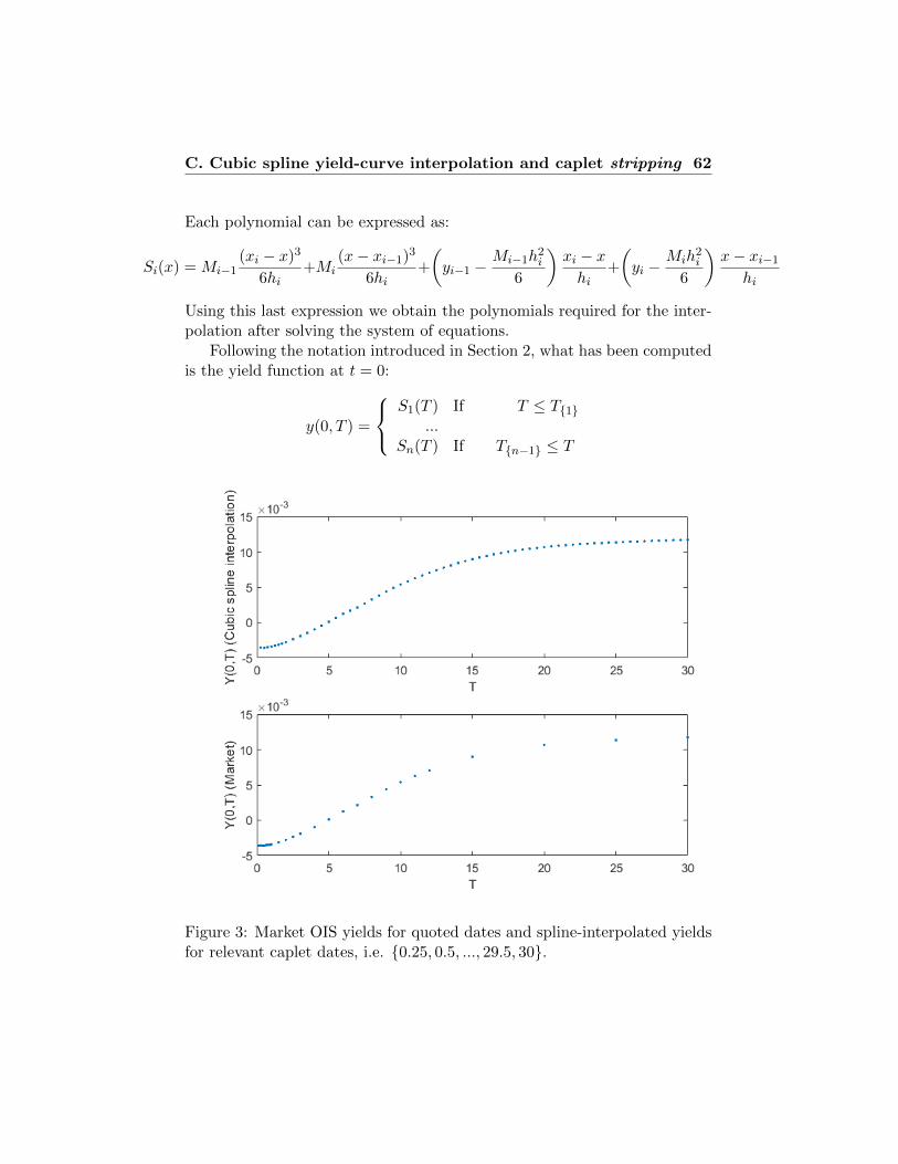
C. Cubic spline yield-curve interpolation and caplet stripping 62
Each polynomial can be expressed as:
Si(x) = Mi−1(xi − x)3
6hi+Mi
(x− xi−1)3
6hi+
(yi−1 −
Mi−1h2i
6
)xi − xhi
+
(yi −
Mih2i
6
)x− xi−1
hi
Using this last expression we obtain the polynomials required for the inter-polation after solving the system of equations.
Following the notation introduced in Section 2, what has been computedis the yield function at t = 0:
y(0, T ) =
S1(T ) If T ≤ T{1}
...Sn(T ) If T{n−1} ≤ T
Figure 3: Market OIS yields for quoted dates and spline-interpolated yieldsfor relevant caplet dates, i.e. {0.25, 0.5, ..., 29.5, 30}.

C. Cubic spline yield-curve interpolation and caplet stripping 63
This allows to compute t = 0 bond prices for every maturity (by rela-tionship (1)):
P (0, T ) = exp
(− T y(0, T )
)Caplet stripping
A bootstrapping technique will be used to infer caplet volatilities, whichinvolves finding iteratively the implied volatility that makes equal the sumof cap prices up to a certain date with the quoted volatility, and the sum ofcaplet prices using a different volatility for each set of caplets between capmaturities. The process allows for the recovery of caplet volatilities for everystrike except ATM37. As noted in Section 6, we will focus on a single strikefor calibration. The results for caplets with strike k = 0.005 are shown inFigure 4. Having recovered caplet implied volatilities, it is straightforwardto obtain caplet prices by means of the Bachelier formula.
Figure 4: Stripped Bachelier volatilities for caplets with maturitiesTmaturity,caplets ∈ {0.5, 0.75, 1, 1.25, ..., 28, 28.5, 29, 29.5, 30} and k = 0.005
37The ATM volatility won’t be considered for simplicity, although is a liquid part ofthe market. The strike in this case is by definition equal to the swap rate being thenmaturity-varying, which adds a layer of complexity. It requires the calculation of pricesfor strikes not quoted in the market and therefore a strike-interpolating method is needed,as noted in [Atanasova, 2017].
REFERENCES 64
References
[Acar, 2009] Acar, S. (2009). A guide on the implementation of the Heath-Jarrow-Morton TwoFactor Gaussian Short Rate Model. Berichte desFraunhofer ITWM, Nr. 170.
[Atanasova, 2017] Atanasova, E. (2017). Pricing and Hedging Fixed IncomeDerivatives under Negative Interest Rates: An SABR approach. Master’sThesis, Universidad Complutense de Madrid.
[Baxter and Rennie, 1996] Baxter, M. and Rennie, A. (1996). Financialcalculus: An introduction to derivative pricing. Cambridge UniversityPress.
[Beyna, 2013] Beyna, I. (2013). Interest Rate Derivatives: Valua-tion,Calibration and Sensitivity Analysis. Springer.
[Brigo and Mercurio, 2006] Brigo, D. and Mercurio, F. (2006). Interest RateModels: Theory and Practice. Springer Finance.
[Broadie and Glasserman, 1997] Broadie, M. and Glasserman, P. (1997).Pricing american-style securities using simulation. Journal of EconomicsDynamics and Control, (21):1323 – 1352.
[Broadie and Glasserman, 2004] Broadie, M. and Glasserman, P. (2004). Astochastic mesh method for pricing high-dimensional american options.The Journal of Computational Finance, 7(4):35 – 72.
[Cairns, 2004] Cairns, A. (2004). Interest Rate Models: An Introduction.Princeton University Press.
[Carverhill, 1994] Carverhill, A. (1994). When is the short rate markovian?Mathematical Finance, 4(4):305 – 312.
[Cheyette, 1994] Cheyette, O. (1994). Markov Representation of the Heath-Jarrow-Morton Model. Presented at the UCLA Workshop on the Futureof Fixed Income Financial Theory.
[Filipovic, 2009] Filipovic, D. (2009). Term Structure Models: A GraduateCourse. Springer Finance.
[Glasserman, 2003] Glasserman, P. (2003). Monte Carlo Methods in Finan-cial Engineering. Springer.
REFERENCES 65
[Heath et al., 1992] Heath, D. et al. (1992). Bond pricing and the termstructure of interest methodology for contingent claims valuation. Econo-metrica, 60(1):77 – 105.
[Holton, 2003] Holton, G. (2003). Value at Risk: Theory and Practice. Aca-demic Press.
[Longstaff and Schwartz, 2001] Longstaff, F. and Schwartz, E. (2001). Valu-ing american options by simulation: A simple least-squares approach. TheReview of Financial Studies, 14(1):113 – 147.
[Musiela and Rutkowski, 1997] Musiela, M. and Rutkowski, M. (1997).Martingale Methods in Financial Modelling. Springer.
[Pliska, 1997] Pliska, S. (1997). Introduction to Mathematical Finance: Dis-crete time models. John Wiley and Sons.
[Press et al., 2007] Press, H. et al. (2007). Numerical Recipes: The Art ofScientific Computing (third edition). Cambridge University Press.
[Privault, 2018] Privault, N. (2018). Notes on Stochastic Finance. NanyangTechnological University.
[Protter, 2003] Protter, P. (2003). Stochastic Integration and DifferentialEquations. Springer.
[Ritchken et al., 1995] Ritchken, P. et al. (1995). Volatility structures offorward rates and the dynamics of the term structure. MathematicalFinance, 1(5):55 – 72.
[Sondermann, 2006] Sondermann, D. (2006). Introduction to Stochastic Cal-culus for Finance: A new didactic approach. Springer.
[Valero et al., 2011] Valero, E. et al. (2011). Fast resolution of a single factorheath-jarrow-morton model with stochastic volatility. Journal of Compu-tational and Applied Mathematics, (236):1637 – 1655.
[Wikiversity, 2019] Wikiversity (2019). Cubic spline interpolation.


![New arXiv:cond-mat/0206457v1 [cond-mat.soft] 24 Jun 2002 · 2018. 11. 15. · A quantum field theory generalization, Baaquie [1], of the Heath, Jarrow, and Morton (HJM) [10] term](https://img.pdfslide.net/doc/110x75/6067d2d885b33078ba040f04/new-arxivcond-mat0206457v1-cond-matsoft-24-jun-2002-2018-11-15-a-quantum.jpg)


![A QUANTUM FIELD THEORY TERM STRUCTURE MODEL APPLIED …srikant.org/ijtaf.pdf · 2009. 12. 1. · A quantum eld theory generalization, Baaquie [1], of the Heath, Jarrow and Morton](https://img.pdfslide.net/doc/110x75/6067d04baa3de15eae43e58e/a-quantum-field-theory-term-structure-model-applied-2009-12-1-a-quantum-eld.jpg)