Embed Size (px)
Citation preview
FIN501 Asset PricingLecture 04 Risk Prefs & EU (1)
LECTURE 4: RISK PREFERENCES & EXPECTED UTILITY THEORY
Markus K. Brunnermeier
FIN501 Asset PricingLecture 04 Risk Prefs & EU (2)
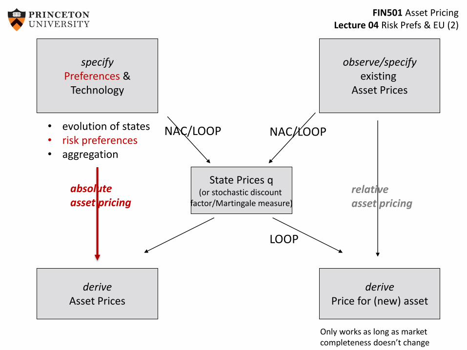
specifyPreferences &
Technology
observe/specifyexisting
Asset Prices
State Prices q(or stochastic discount
factor/Martingale measure)
derivePrice for (new) asset
• evolution of states• risk preferences• aggregation
absolute asset pricing
relativeasset pricing
NAC/LOOP
LOOP
NAC/LOOP
Only works as long as market completeness doesn’t change
deriveAsset Prices
FIN501 Asset PricingLecture 04 Risk Prefs & EU (3)
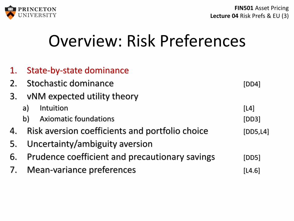
Overview: Risk Preferences
1. State-by-state dominance
2. Stochastic dominance [DD4]
3. vNM expected utility theorya) Intuition [L4]
b) Axiomatic foundations [DD3]
4. Risk aversion coefficients and portfolio choice [DD5,L4]
5. Uncertainty/ambiguity aversion
6. Prudence coefficient and precautionary savings [DD5]
7. Mean-variance preferences [L4.6]
FIN501 Asset PricingLecture 04 Risk Prefs & EU (4)
State-by-state Dominance
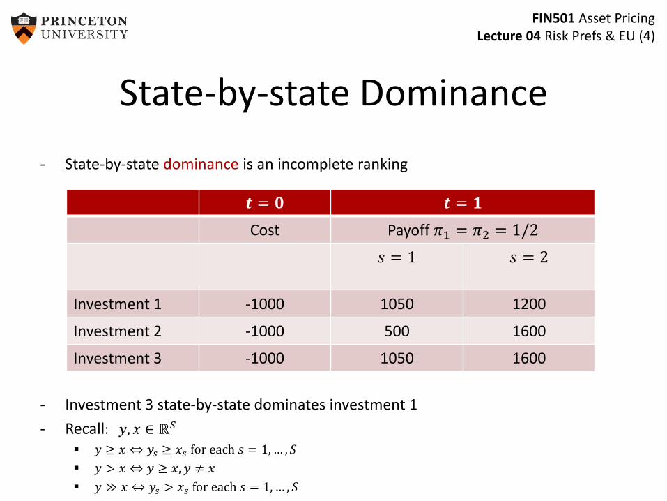
- State-by-state dominance is an incomplete ranking
- Investment 3 state-by-state dominates investment 1
- Recall: 𝑦, 𝑥 ∈ ℝ𝑆
𝑦 ≥ 𝑥 ⇔ 𝑦𝑠 ≥ 𝑥𝑠 for each 𝑠 = 1,… , 𝑆
𝑦 > 𝑥 ⇔ 𝑦 ≥ 𝑥, 𝑦 ≠ 𝑥
𝑦 ≫ 𝑥 ⇔ 𝑦𝑠 > 𝑥𝑠 for each 𝑠 = 1,… , 𝑆
𝒕 = 𝟎 𝒕 = 𝟏
Cost Payoff 𝜋1 = 𝜋2 = 1/2
𝑠 = 1 𝑠 = 2
Investment 1 -1000 1050 1200
Investment 2 -1000 500 1600
Investment 3 -1000 1050 1600
FIN501 Asset PricingLecture 04 Risk Prefs & EU (5)
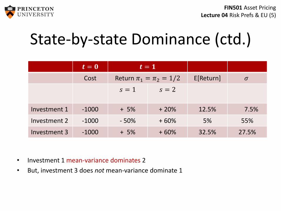
State-by-state Dominance (ctd.)
• Investment 1 mean-variance dominates 2
• But, investment 3 does not mean-variance dominate 1
𝒕 = 𝟎 𝒕 = 𝟏
Cost Return 𝜋1 = 𝜋2 = 1/2 E[Return] 𝜎
𝑠 = 1 𝑠 = 2
Investment 1 -1000 + 5% + 20% 12.5% 7.5%
Investment 2 -1000 - 50% + 60% 5% 55%
Investment 3 -1000 + 5% + 60% 32.5% 27.5%
FIN501 Asset PricingLecture 04 Risk Prefs & EU (6)
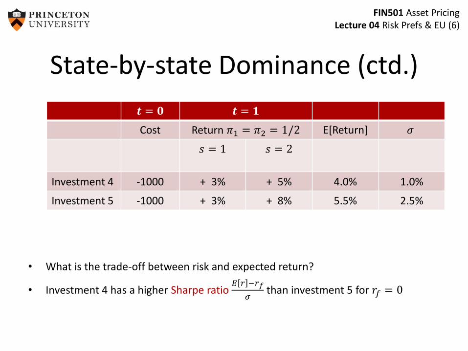
State-by-state Dominance (ctd.)
• What is the trade-off between risk and expected return?
• Investment 4 has a higher Sharpe ratio 𝐸 𝑟 −𝑟𝑓
𝜎than investment 5 for 𝑟𝑓 = 0
𝒕 = 𝟎 𝒕 = 𝟏
Cost Return 𝜋1 = 𝜋2 = 1/2 E[Return] 𝜎
𝑠 = 1 𝑠 = 2
Investment 4 -1000 + 3% + 5% 4.0% 1.0%
Investment 5 -1000 + 3% + 8% 5.5% 2.5%
FIN501 Asset PricingLecture 04 Risk Prefs & EU (7)
Overview: Risk Preferences
1. State-by-state dominance
2. Stochastic dominance [DD4]
3. vNM expected utility theorya) Intuition [L4]
b) Axiomatic foundations [DD3]
4. Risk aversion coefficients and portfolio choice [DD5,L4]
5. Prudence coefficient and precautionary savings [DD5]
6. Mean-variance preferences [L4.6]
FIN501 Asset PricingLecture 04 Risk Prefs & EU (8)
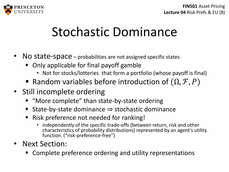
Stochastic Dominance
• No state-space – probabilities are not assigned specific states
Only applicable for final payoff gamble • Not for stocks/lotteries that form a portfolio (whose payoff is final)
Random variables before introduction of (Ω, ℱ, 𝑃)• Still incomplete ordering
“More complete” than state-by-state ordering State-by-state dominance ⇒ stochastic dominance Risk preference not needed for ranking!
• independently of the specific trade-offs (between return, risk and other characteristics of probability distributions) represented by an agent's utility function. (“risk-preference-free”)
• Next Section: Complete preference ordering and utility representations
FIN501 Asset PricingLecture 04 Risk Prefs & EU (9)
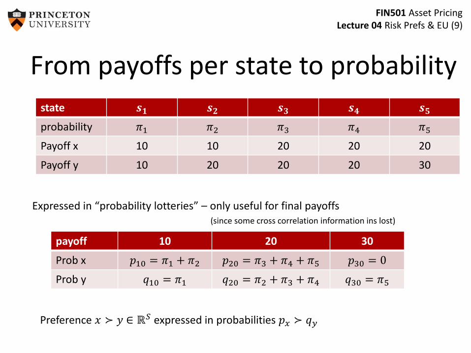
From payoffs per state to probability
state 𝒔𝟏 𝒔𝟐 𝒔𝟑 𝒔𝟒 𝒔𝟓
probability 𝜋1 𝜋2 𝜋3 𝜋4 𝜋5
Payoff x 10 10 20 20 20
Payoff y 10 20 20 20 30
payoff 10 20 30
Prob x 𝑝10 = 𝜋1 + 𝜋2 𝑝20 = 𝜋3 + 𝜋4 + 𝜋5 𝑝30 = 0
Prob y 𝑞10 = 𝜋1 𝑞20 = 𝜋2 + 𝜋3 + 𝜋4 𝑞30 = 𝜋5
Expressed in “probability lotteries” – only useful for final payoffs (since some cross correlation information ins lost)
Preference 𝑥 ≻ 𝑦 ∈ ℝ𝑆 expressed in probabilities 𝑝𝑥 ≻ 𝑞𝑦
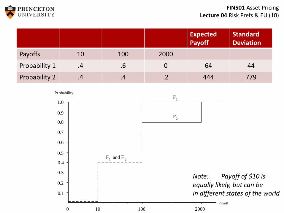
FIN501 Asset PricingLecture 04 Risk Prefs & EU (10)
0 10 100 2000
0.1
0.4
0.2
0.3
0.5
0.6
0.7
0.8
0.9
1.0
F1
and F2
F1
F2
Payoff
obabilityPr
ExpectedPayoff
Standard Deviation
Payoffs 10 100 2000
Probability 1 .4 .6 0 64 44
Probability 2 .4 .4 .2 444 779
Note: Payoff of $10 is equally likely, but can bein different states of the world
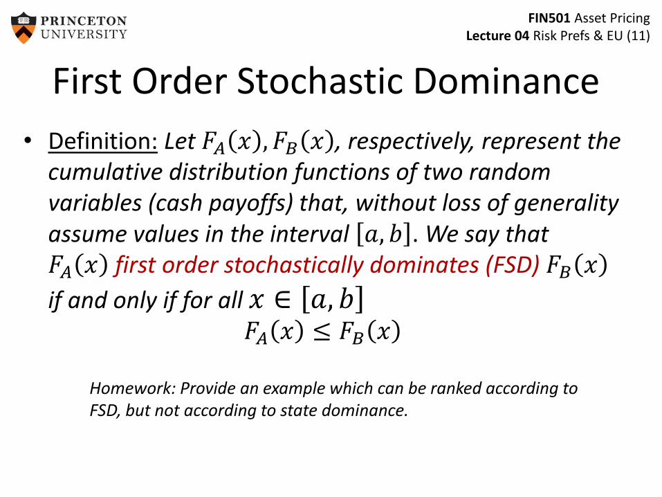
FIN501 Asset PricingLecture 04 Risk Prefs & EU (11)
• Definition: Let 𝐹𝐴 𝑥 , 𝐹𝐵 𝑥 , respectively, represent the cumulative distribution functions of two random variables (cash payoffs) that, without loss of generality assume values in the interval 𝑎, 𝑏 . We say that 𝐹𝐴 𝑥 first order stochastically dominates (FSD) 𝐹𝐵 𝑥
if and only if for all 𝑥 ∈ 𝑎, 𝑏𝐹𝐴 𝑥 ≤ 𝐹𝐵 𝑥
Homework: Provide an example which can be ranked according to FSD, but not according to state dominance.
First Order Stochastic Dominance
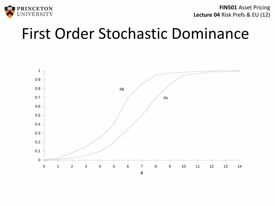
FIN501 Asset PricingLecture 04 Risk Prefs & EU (12)
X
0
0.1
0.2
0.3
0.4
0.5
0.6
0.7
0.8
0.9
1
0 1 2 3 4 5 6 7 8 9 10 11 12 13 14
FA
FB
First Order Stochastic Dominance

FIN501 Asset PricingLecture 04 Risk Prefs & EU (13)
0
0.1
0.2
0.3
0.4
0.5
0.6
0.7
0.8
0.9
1
0 1 2 3 4 5 6 7 8 9 10 11 12 13
investment 3
investment 4
CDFs of investment 3 and 4
Payoff 1 4 5 6 8 12
Probability 3 0 .25 0.50 0 0 .25
Probability 4 .33 0 0 .33 .33 0
FIN501 Asset PricingLecture 04 Risk Prefs & EU (14)
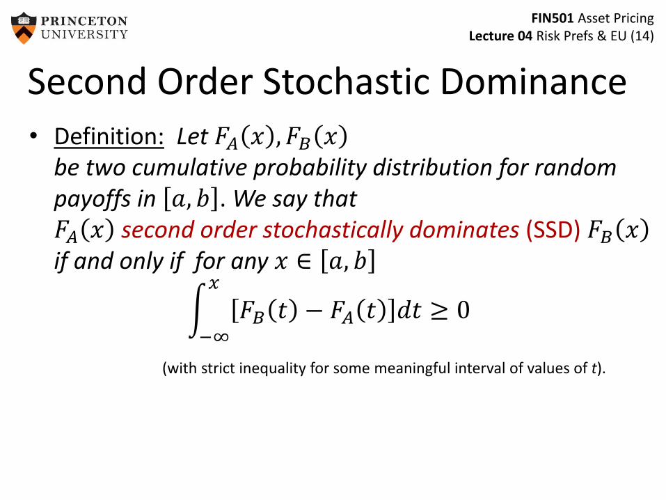
• Definition: Let 𝐹𝐴 𝑥 , 𝐹𝐵 𝑥be two cumulative probability distribution for random payoffs in 𝑎, 𝑏 . We say that 𝐹𝐴 𝑥 second order stochastically dominates (SSD) 𝐹𝐵 𝑥if and only if for any 𝑥 ∈ 𝑎, 𝑏
−∞
𝑥
𝐹𝐵 𝑡 − 𝐹𝐴 𝑡 𝑑𝑡 ≥ 0
(with strict inequality for some meaningful interval of values of t).
Second Order Stochastic Dominance
FIN501 Asset PricingLecture 04 Risk Prefs & EU (15)
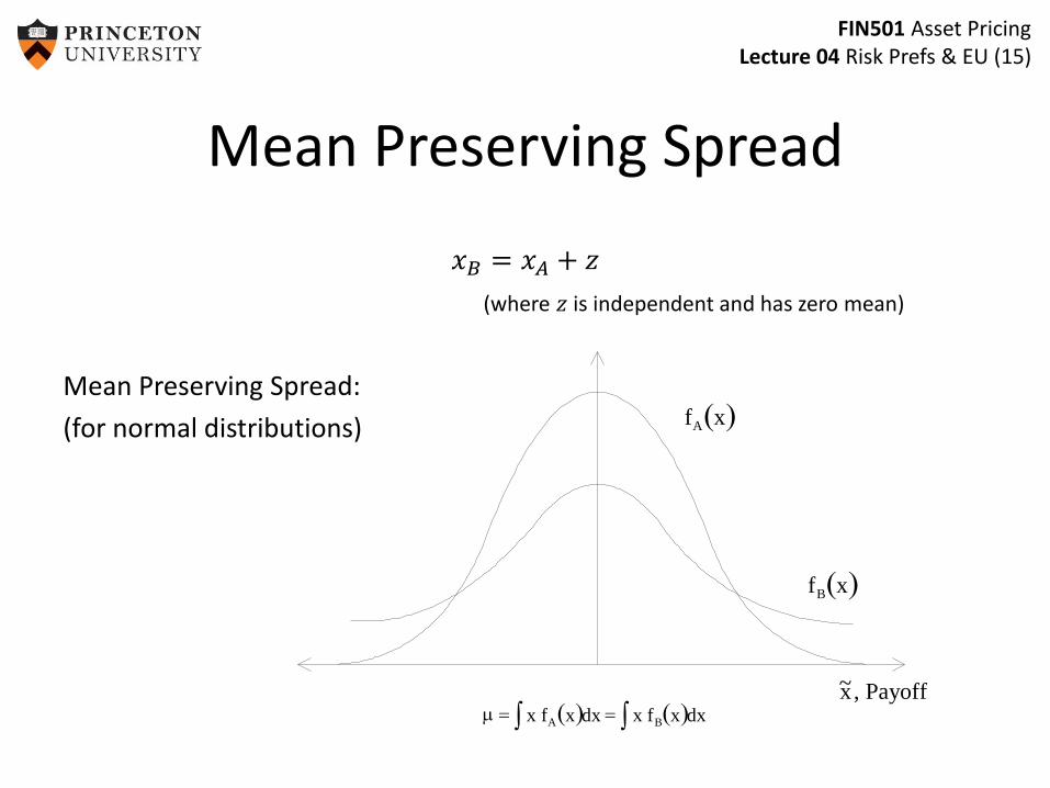
f xA
f xB
~,x Payoff x f x dx x f x dxA B
Mean Preserving Spread
𝑥𝐵 = 𝑥𝐴 + 𝑧
(where 𝑧 is independent and has zero mean)
Mean Preserving Spread:
(for normal distributions)
FIN501 Asset PricingLecture 04 Risk Prefs & EU (16)
• Theorem: Let 𝐹𝐴 𝑥 and 𝐹𝐵 𝑥 be two distribution functions defined on the same state space with identical means. Then the following statements are equivalent :
𝐹𝐴 𝑥 SSD 𝐹𝐵 𝑥
𝐹𝐵 𝑥 is a mean-preserving spread of 𝐹𝐴 𝑥
Mean Preserving Spread & SSD
FIN501 Asset PricingLecture 04 Risk Prefs & EU (17)
Overview: Risk Preferences
1. State-by-state dominance
2. Stochastic dominance [DD4]
3. vNM expected utility theorya) Intuition [L4]
b) Axiomatic foundations [DD3]
4. Risk aversion coefficients and portfolio choice [DD5,L4]
5. Prudence coefficient and precautionary savings [DD5]
6. Mean-variance preferences [L4.6]
FIN501 Asset PricingLecture 04 Risk Prefs & EU (18)
A Hypothetical Gamble
• Suppose someone offers you this gamble: "I have a fair coin here. I'll flip it, and if it's tails I
pay you $1 and the gamble is over. If it's heads, I'll flip again. If it's tails then, I pay you $2, if not I'll flip again. With every round, I double the amount I will pay to you if it turns up tails."
• Sounds like a good deal. After all, you can't lose. So here's the question: How much are you willing to pay to take this
gamble?
FIN501 Asset PricingLecture 04 Risk Prefs & EU (19)
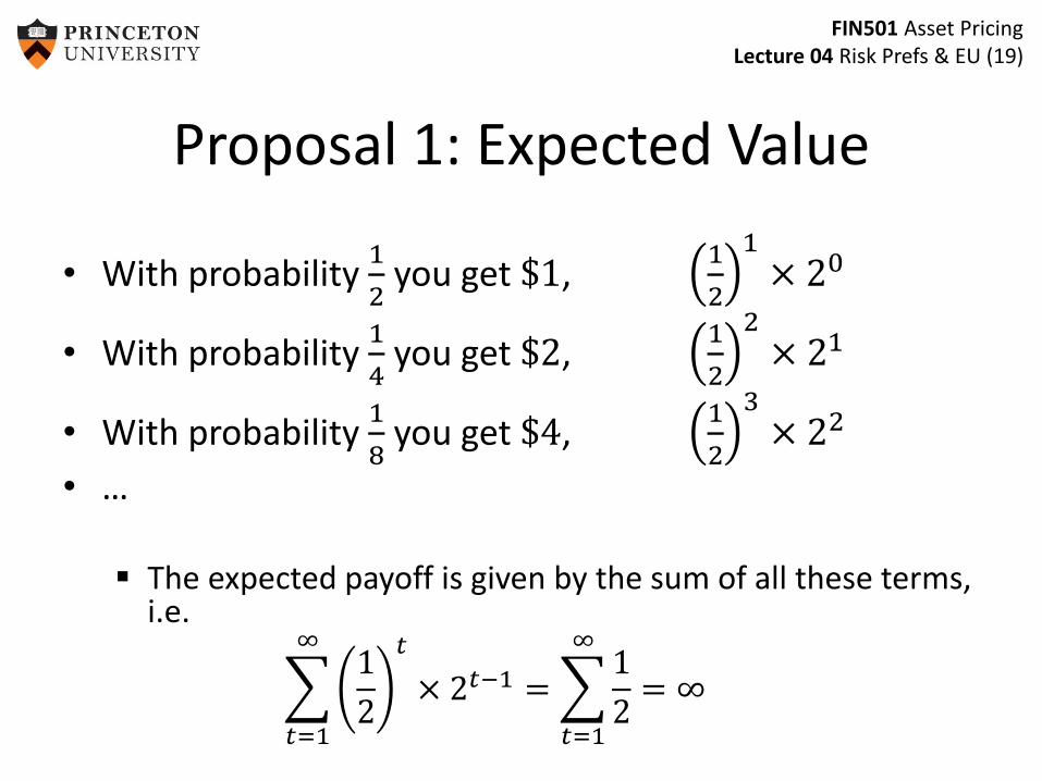
Proposal 1: Expected Value
• With probability 1
2you get $1,
1
2
1× 20
• With probability 1
4you get $2,
1
2
2× 21
• With probability 1
8you get $4,
1
2
3× 22
• …
The expected payoff is given by the sum of all these terms, i.e.
𝑡=1
∞1
2
𝑡
× 2𝑡−1 =
𝑡=1
∞1
2= ∞
FIN501 Asset PricingLecture 04 Risk Prefs & EU (20)
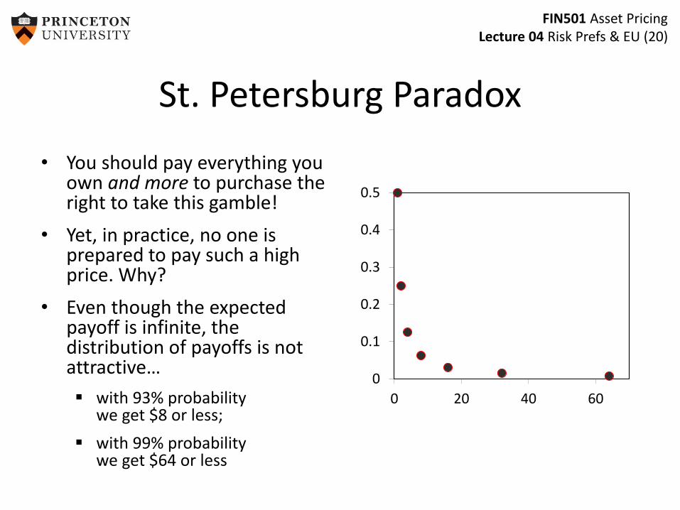
St. Petersburg Paradox
• You should pay everything you own and more to purchase the right to take this gamble!
• Yet, in practice, no one is prepared to pay such a high price. Why?
• Even though the expected payoff is infinite, the distribution of payoffs is not attractive…
with 93% probability we get $8 or less;
with 99% probability we get $64 or less
0
0.1
0.2
0.3
0.4
0.5
0 20 40 60
FIN501 Asset PricingLecture 04 Risk Prefs & EU (21)
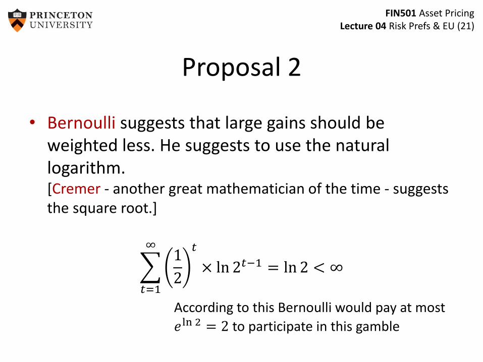
Proposal 2
• Bernoulli suggests that large gains should be weighted less. He suggests to use the natural logarithm. [Cremer - another great mathematician of the time - suggests the square root.]
𝑡=1
∞1
2
𝑡
× ln 2𝑡−1 = ln 2 < ∞
According to this Bernoulli would pay at most
𝑒ln 2 = 2 to participate in this gamble
FIN501 Asset PricingLecture 04 Risk Prefs & EU (22)
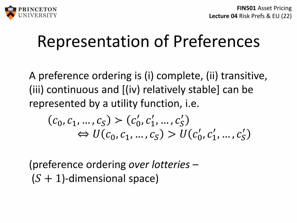
Representation of Preferences
A preference ordering is (i) complete, (ii) transitive, (iii) continuous and [(iv) relatively stable] can be represented by a utility function, i.e.
𝑐0, 𝑐1, … , 𝑐𝑆 ≻ 𝑐0′ , 𝑐1
′ , … , 𝑐𝑆′
⇔ 𝑈 𝑐0, 𝑐1, … , 𝑐𝑆 > 𝑈 𝑐0′ , 𝑐1
′ , … , 𝑐𝑆′
(preference ordering over lotteries –(𝑆 + 1)-dimensional space)
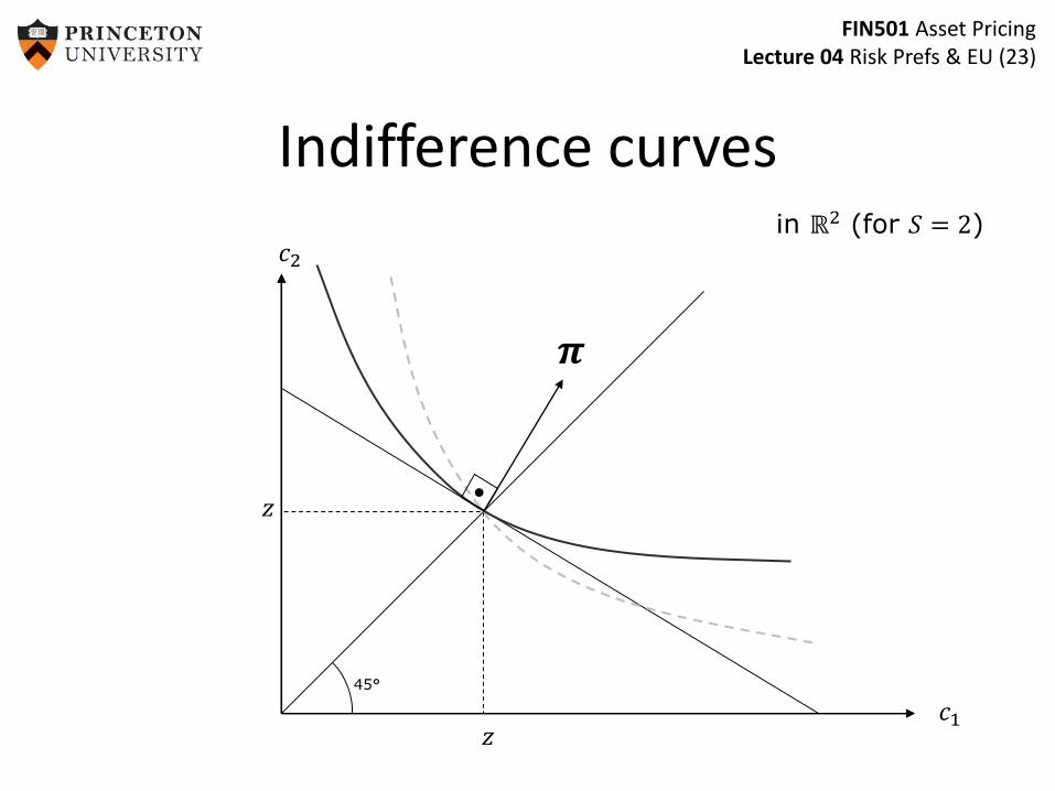
FIN501 Asset PricingLecture 04 Risk Prefs & EU (23)
Indifference curvesin ℝ2 (for 𝑆 = 2)
45°
𝑐1
𝑐2
𝝅
𝑧
𝑧
FIN501 Asset PricingLecture 04 Risk Prefs & EU (24)
Preferences over Prob. Distributions
• Consider 𝑐0 fixed, 𝑐1 is a random variable
• Preference ordering over probability distributions
• Let
𝑃 be a set of probability distributions with a finite support over a set 𝑋,
≽ preference ordering over 𝑃 (that is, a subset of 𝑃 × 𝑃)
FIN501 Asset PricingLecture 04 Risk Prefs & EU (25)
Prob. Distributions
• S states of the world• Set of all possible lotteries
𝑃 = 𝑝 ∈ ℝ𝑆 𝑝 𝑐 ≥ 0, 𝑝 𝑐 = 1
• Space with S dimensions
• Can we simplify the utility representation of preferences over lotteries?
• Space with one dimension – income• We need to assume further axioms
FIN501 Asset PricingLecture 04 Risk Prefs & EU (26)
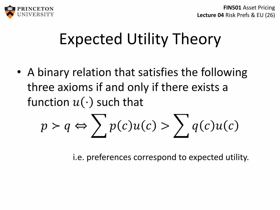
Expected Utility Theory
• A binary relation that satisfies the following three axioms if and only if there exists a function 𝑢 ⋅ such that
𝑝 ≻ 𝑞 ⇔ 𝑝 𝑐 𝑢 𝑐 > 𝑞 𝑐 𝑢 𝑐
i.e. preferences correspond to expected utility.
FIN501 Asset PricingLecture 04 Risk Prefs & EU (27)
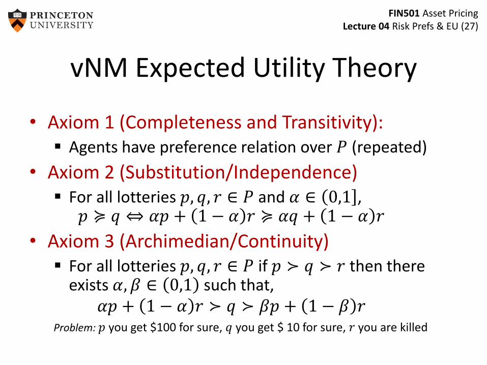
vNM Expected Utility Theory
• Axiom 1 (Completeness and Transitivity): Agents have preference relation over 𝑃 (repeated)
• Axiom 2 (Substitution/Independence) For all lotteries 𝑝, 𝑞, 𝑟 ∈ 𝑃 and 𝛼 ∈ 0,1 ,
𝑝 ≽ 𝑞 ⇔ 𝛼𝑝 + 1 − 𝛼 𝑟 ≽ 𝛼𝑞 + 1 − 𝛼 𝑟
• Axiom 3 (Archimedian/Continuity) For all lotteries 𝑝, 𝑞, 𝑟 ∈ 𝑃 if 𝑝 ≻ 𝑞 ≻ 𝑟 then there
exists 𝛼, 𝛽 ∈ 0,1 such that,𝛼𝑝 + 1 − 𝛼 𝑟 ≻ 𝑞 ≻ 𝛽𝑝 + 1 − 𝛽 𝑟
Problem: 𝑝 you get $100 for sure, 𝑞 you get $ 10 for sure, 𝑟 you are killed
FIN501 Asset PricingLecture 04 Risk Prefs & EU (28)
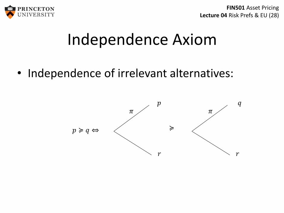
Independence Axiom
• Independence of irrelevant alternatives:
𝑝 ≽ 𝑞 ⇔
𝜋 𝜋𝑝
𝑟 𝑟
𝑞
≽
FIN501 Asset PricingLecture 04 Risk Prefs & EU (29)
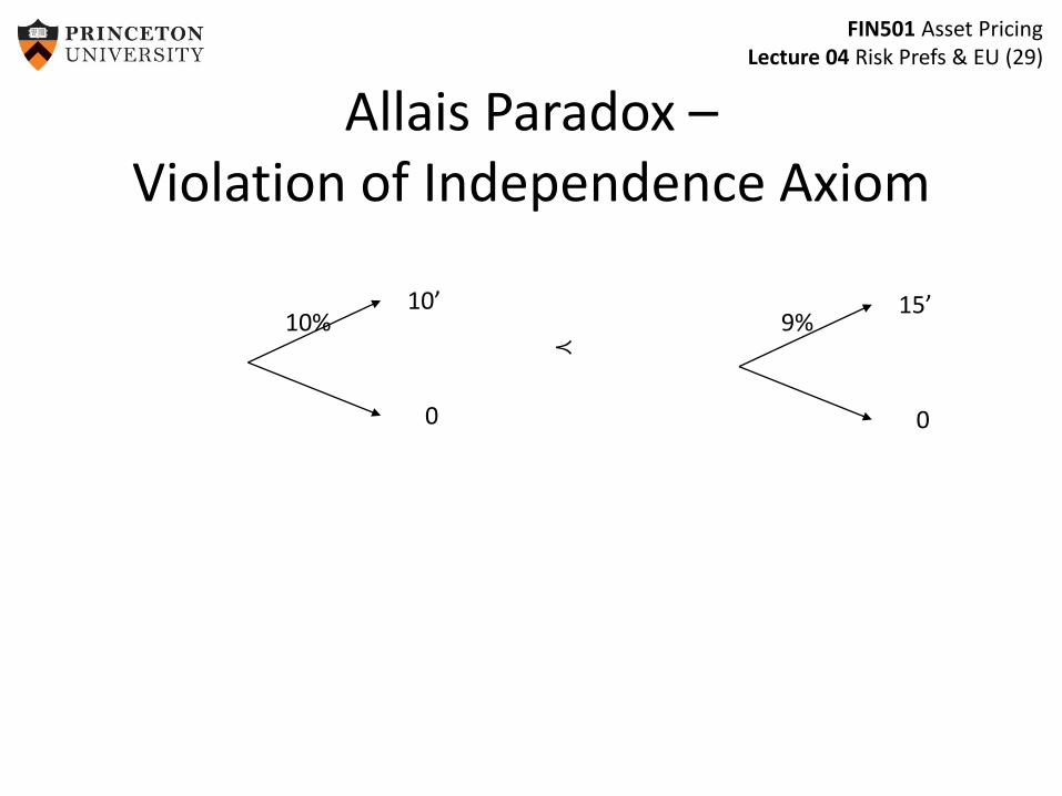
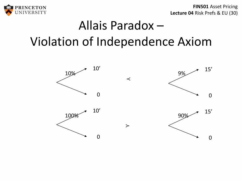
Allais Paradox –Violation of Independence Axiom
10’
0
15’
0
9%10%≺
FIN501 Asset PricingLecture 04 Risk Prefs & EU (30)
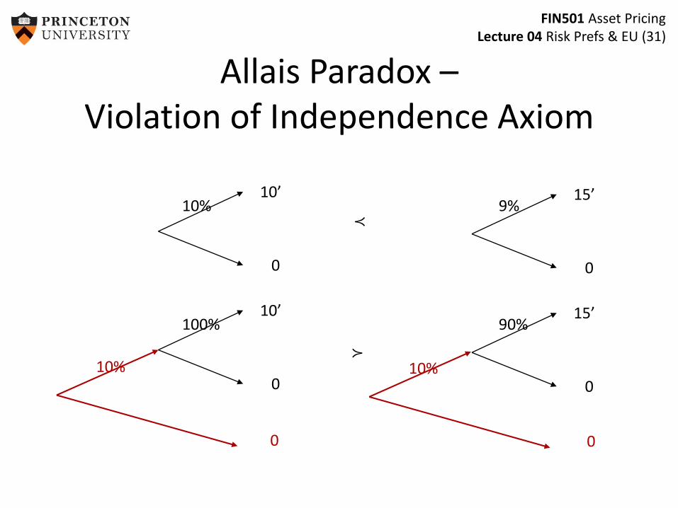
Allais Paradox –Violation of Independence Axiom
10’
0
15’
0
9%10%≺
10’
0
15’
0
90%100%
≻
FIN501 Asset PricingLecture 04 Risk Prefs & EU (31)
10’
0
15’
0
9%10%≺
10’
0
15’
0
90%100%
≻10%
0
10%
0
Allais Paradox –Violation of Independence Axiom
FIN501 Asset PricingLecture 04 Risk Prefs & EU (32)
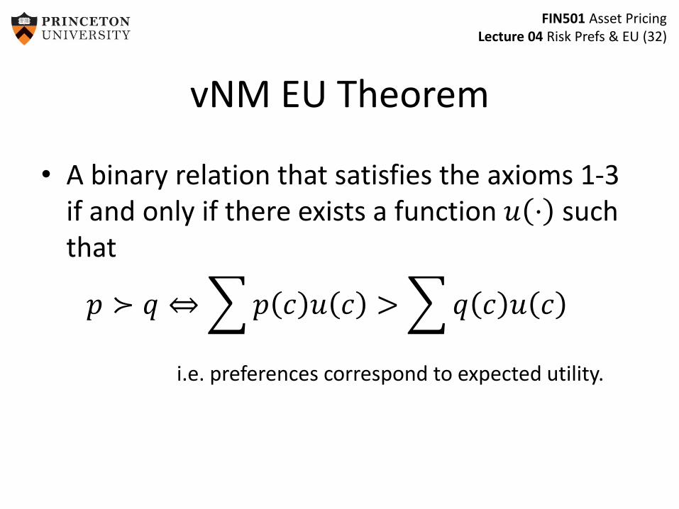
vNM EU Theorem
• A binary relation that satisfies the axioms 1-3 if and only if there exists a function 𝑢 ⋅ such that
𝑝 ≻ 𝑞 ⇔ 𝑝 𝑐 𝑢 𝑐 > 𝑞 𝑐 𝑢 𝑐
i.e. preferences correspond to expected utility.
FIN501 Asset PricingLecture 04 Risk Prefs & EU (33)
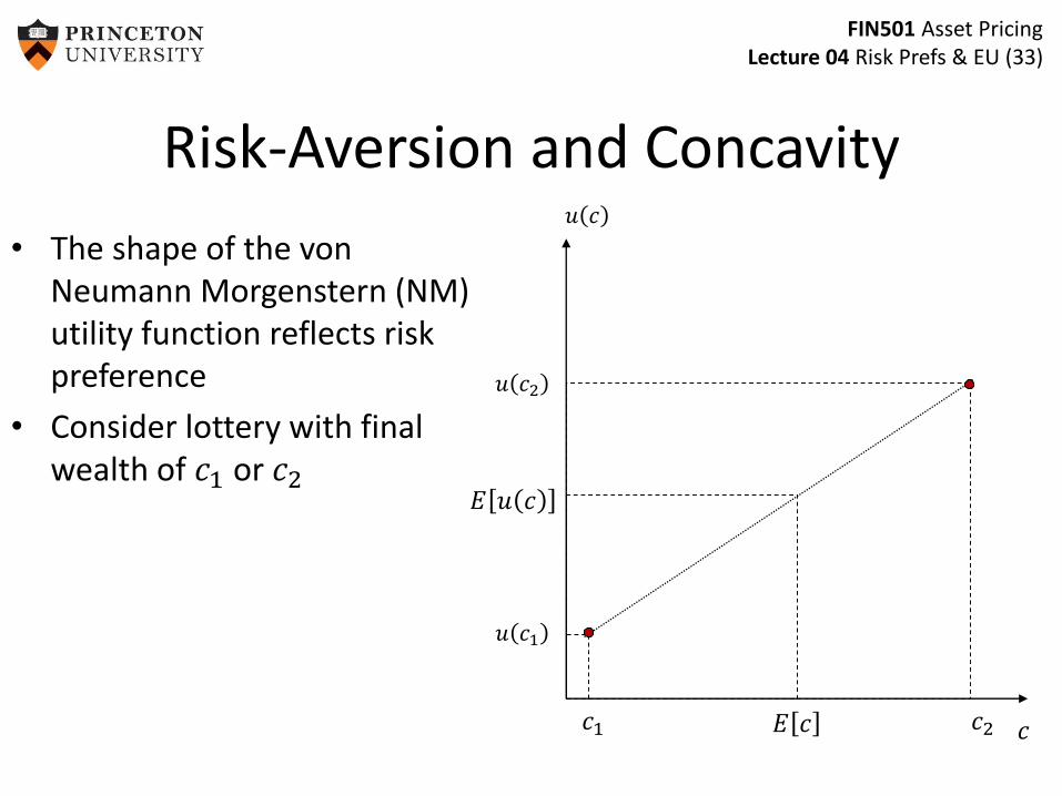
• The shape of the von Neumann Morgenstern (NM) utility function reflects risk preference
• Consider lottery with final wealth of 𝑐1 or 𝑐2
𝐸 𝑢 𝑐
Risk-Aversion and Concavity
𝑐
𝑢 𝑐
𝑐1 𝑐2
𝑢 𝑐1
𝑢 𝑐2
𝐸 𝑐
FIN501 Asset PricingLecture 04 Risk Prefs & EU (34)
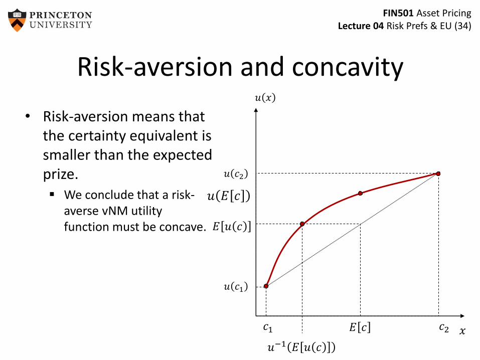
• Risk-aversion means that the certainty equivalent is smaller than the expected prize. We conclude that a risk-
averse vNM utility function must be concave. 𝐸 𝑢 𝑐
Risk-aversion and concavity
𝑥
𝑢 𝑥
𝑐1 𝑐2
𝑢 𝑐1
𝑢 𝑐2
𝐸 𝑐
𝑢−1 𝐸 𝑢 𝑐
𝑢 𝐸 𝑐
FIN501 Asset PricingLecture 04 Risk Prefs & EU (35)
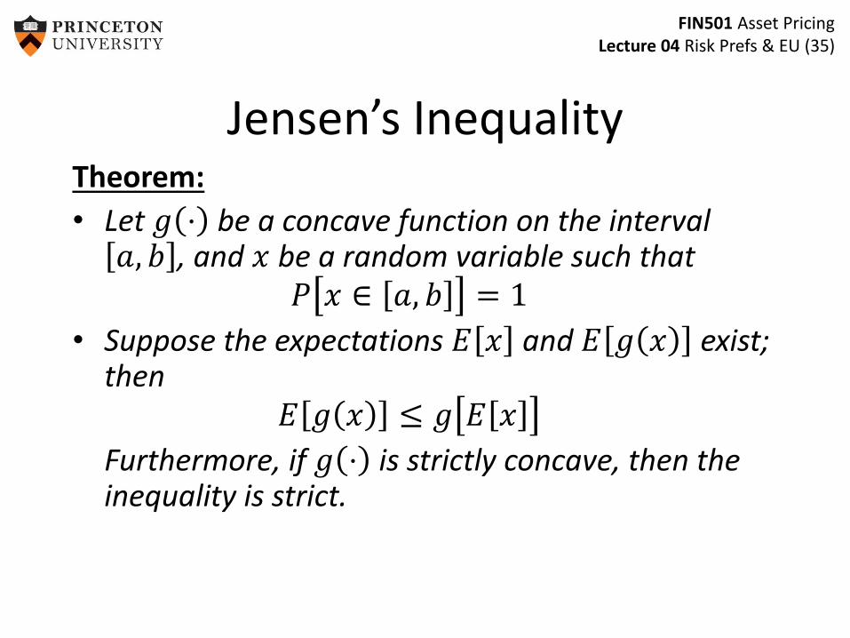
Theorem:
• Let 𝑔 ⋅ be a concave function on the interval 𝑎, 𝑏 , and 𝑥 be a random variable such that
𝑃 𝑥 ∈ 𝑎, 𝑏 = 1
• Suppose the expectations 𝐸 𝑥 and 𝐸 𝑔 𝑥 exist; then
𝐸 𝑔 𝑥 ≤ 𝑔 𝐸 𝑥
Furthermore, if 𝑔 ⋅ is strictly concave, then the inequality is strict.
Jensen’s Inequality
FIN501 Asset PricingLecture 04 Risk Prefs & EU (36)
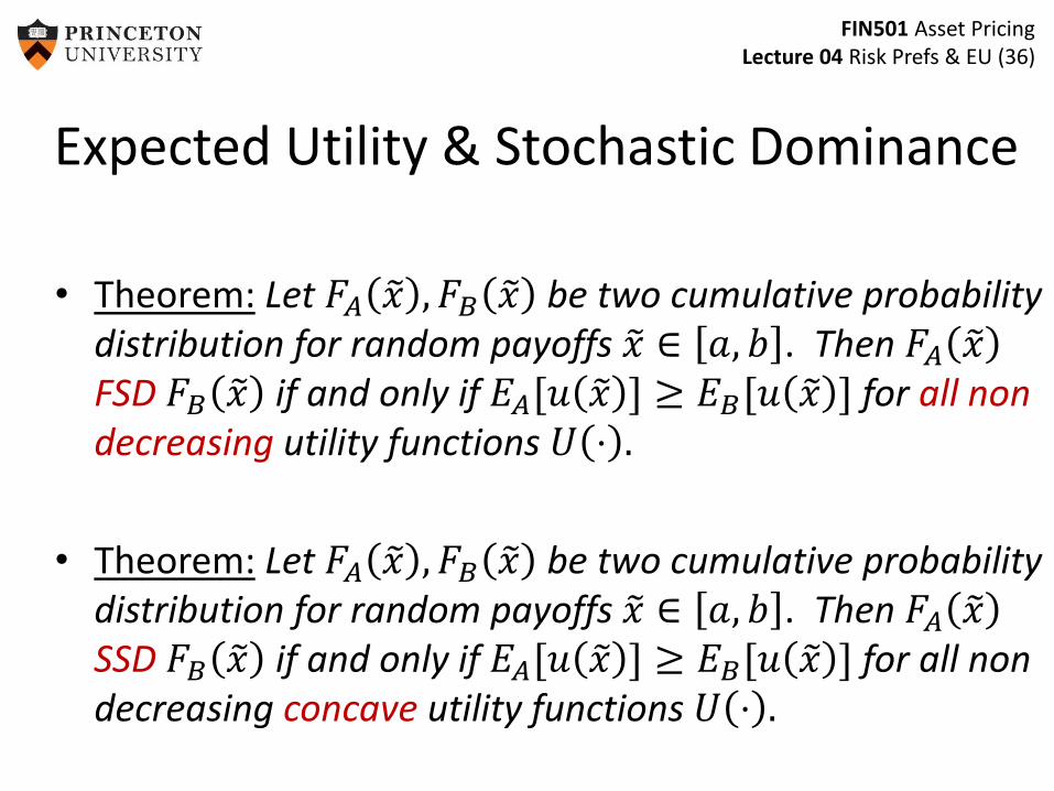
• Theorem: Let 𝐹𝐴 𝑥 , 𝐹𝐵 𝑥 be two cumulative probability distribution for random payoffs 𝑥 ∈ 𝑎, 𝑏 . Then 𝐹𝐴 𝑥FSD 𝐹𝐵 𝑥 if and only if 𝐸𝐴[𝑢 𝑥 ] ≥ 𝐸𝐵[𝑢 𝑥 ] for all non decreasing utility functions 𝑈 ⋅ .
• Theorem: Let 𝐹𝐴 𝑥 , 𝐹𝐵 𝑥 be two cumulative probability distribution for random payoffs 𝑥 ∈ 𝑎, 𝑏 . Then 𝐹𝐴 𝑥SSD 𝐹𝐵 𝑥 if and only if 𝐸𝐴[𝑢 𝑥 ] ≥ 𝐸𝐵[𝑢 𝑥 ] for all non decreasing concave utility functions 𝑈 ⋅ .
Expected Utility & Stochastic Dominance
FIN501 Asset PricingLecture 04 Risk Prefs & EU (37)
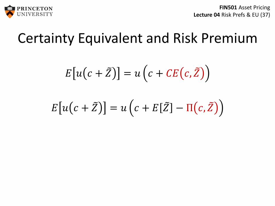
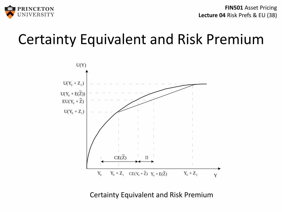
Certainty Equivalent and Risk Premium
𝐸 𝑢 𝑐 + 𝑍 = 𝑢 𝑐 + 𝐶𝐸 𝑐, 𝑍
𝐸 𝑢 𝑐 + 𝑍 = 𝑢 𝑐 + 𝐸 𝑍 − Π 𝑐, 𝑍
FIN501 Asset PricingLecture 04 Risk Prefs & EU (38)
Certainty Equivalent and Risk Premium
Certainty Equivalent and Risk Premium
U(Y)
Y
~
~ ~
P
)ZY(U 20 +
))Z~
(EY(U 0 +
)ZY(EU 0 +
)ZY(U 10 +
)Z~
(CE
0Y 10 ZY + )ZY(CE 0 + )Z(EY0 + 20 ZY +

FIN501 Asset PricingLecture 04 Risk Prefs & EU (39)
Utility Transformations
• General utility function: Suppose 𝑈 𝑐0, 𝑐1, … , 𝑐𝑆 > 𝑈 𝑐0
′ , 𝑐1′ , … , 𝑐𝑆
′ represents complete, transitive,… preference ordering,
then 𝑉 ⋅ = 𝑓 𝑈 ⋅ , where 𝑓 ⋅ is strictly increasingrepresents the same preference ordering
• vNM utility function Suppose 𝐸 𝑢 𝑐 represents preference ordering
satisfying vNM axioms,
then 𝑣 𝑐 = 𝑎 + 𝑏𝑢 𝑐 represents the same.“affine transformation”
FIN501 Asset PricingLecture 04 Risk Prefs & EU (40)
Overview: Risk Preferences
1. State-by-state dominance
2. Stochastic dominance [DD4]
3. vNM expected utility theorya) Intuition [L4]
b) Axiomatic foundations [DD3]
4. Risk aversion coefficients and portfolio choice [DD5,L4]
5. Uncertainty/ambiguity aversion
6. Prudence coefficient and precautionary savings [DD5]
7. Mean-variance preferences [L4.6]
FIN501 Asset PricingLecture 04 Risk Prefs & EU (41)
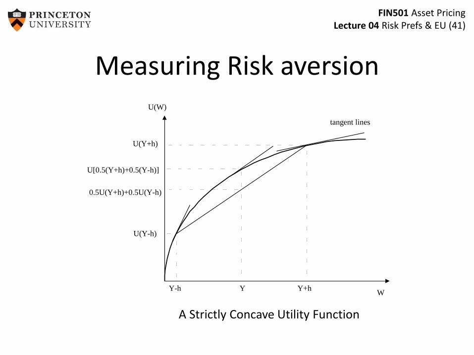
Measuring Risk aversionU(W)
WY-h Y Y+h
U(Y-h)
U[0.5(Y+h)+0.5(Y-h)]
0.5U(Y+h)+0.5U(Y-h)
tangent lines
U(Y+h)
A Strictly Concave Utility Function
FIN501 Asset PricingLecture 04 Risk Prefs & EU (42)
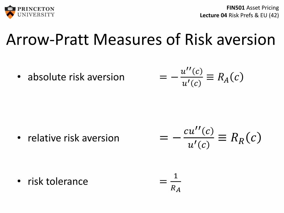
Arrow-Pratt Measures of Risk aversion
• absolute risk aversion = −𝑢′′ 𝑐
𝑢′ 𝑐≡ 𝑅𝐴 𝑐
• relative risk aversion = −𝑐𝑢′′ 𝑐
𝑢′ 𝑐≡ 𝑅𝑅 𝑐
• risk tolerance =1
𝑅𝐴
FIN501 Asset PricingLecture 04 Risk Prefs & EU (43)
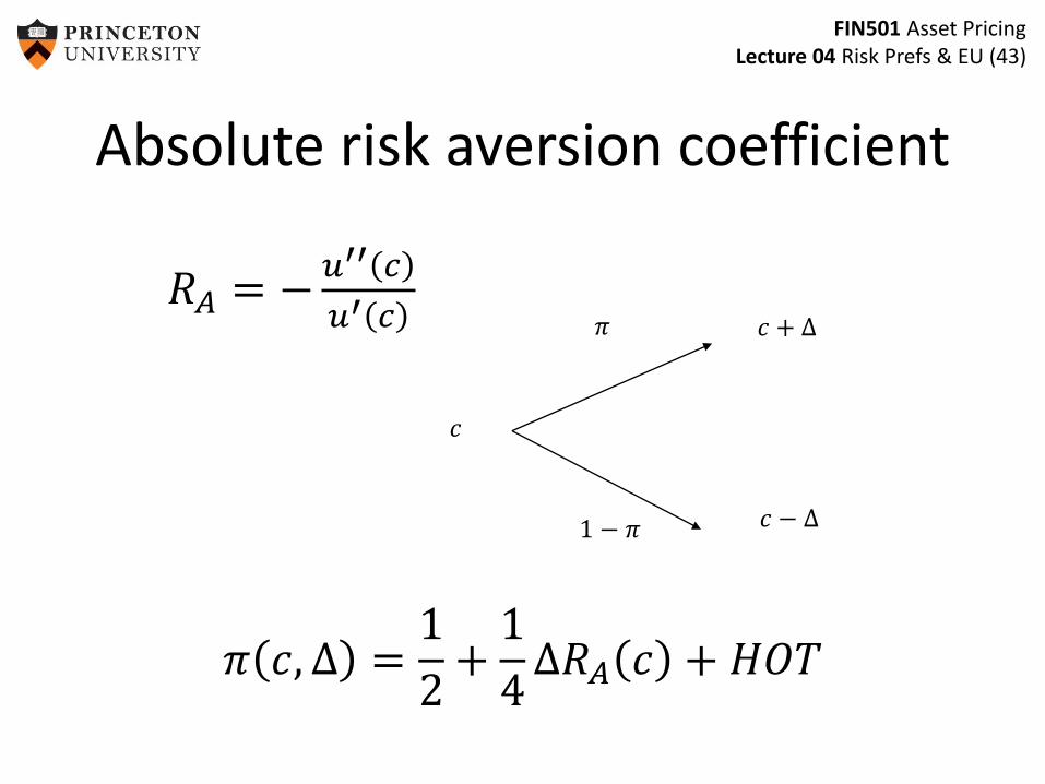
Absolute risk aversion coefficient
𝑅𝐴 = −𝑢′′ 𝑐
𝑢′ 𝑐
𝜋 𝑐, Δ =1
2+
1
4Δ𝑅𝐴 𝑐 + 𝐻𝑂𝑇
𝑐
𝑐 + Δ
𝑐 − Δ
𝜋
1 − 𝜋
FIN501 Asset PricingLecture 04 Risk Prefs & EU (44)
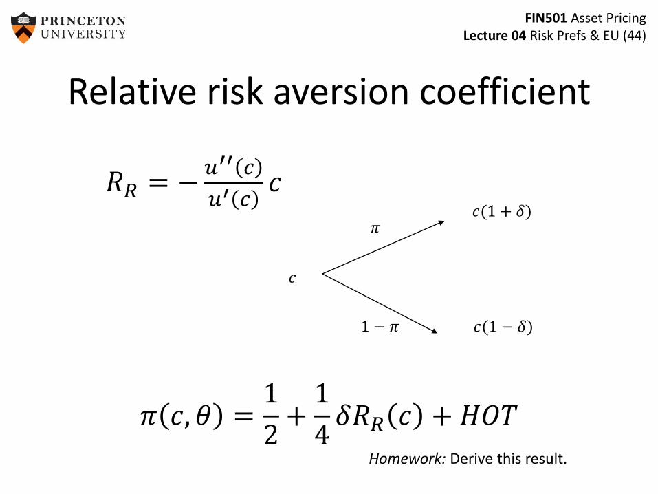
Relative risk aversion coefficient
𝑅𝑅 = −𝑢′′ 𝑐
𝑢′ 𝑐𝑐
𝜋 𝑐, 𝜃 =1
2+
1
4𝛿𝑅𝑅 𝑐 + 𝐻𝑂𝑇
Homework: Derive this result.
𝑐
𝑐(1 + 𝛿)
𝑐(1 − 𝛿)
𝜋
1 − 𝜋
FIN501 Asset PricingLecture 04 Risk Prefs & EU (45)
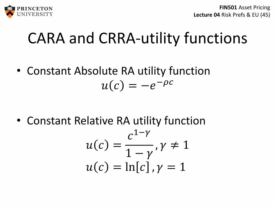
CARA and CRRA-utility functions
• Constant Absolute RA utility function𝑢 𝑐 = −𝑒−𝜌𝑐
• Constant Relative RA utility function
𝑢 𝑐 =𝑐1−𝛾
1 − 𝛾, 𝛾 ≠ 1
𝑢 𝑐 = ln 𝑐 , 𝛾 = 1
FIN501 Asset PricingLecture 04 Risk Prefs & EU (46)
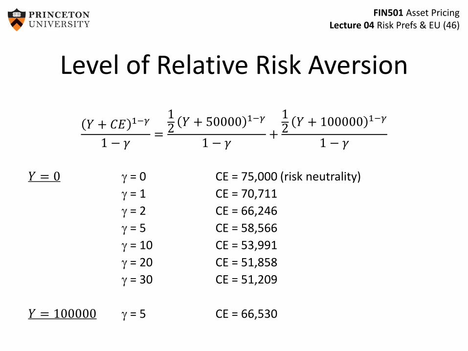
Level of Relative Risk Aversion
𝑌 + 𝐶𝐸 1−𝛾
1 − 𝛾=
12
𝑌 + 50000 1−𝛾
1 − 𝛾+
12
𝑌 + 100000 1−𝛾
1 − 𝛾
𝑌 = 0 = 0 CE = 75,000 (risk neutrality)
= 1 CE = 70,711
= 2 CE = 66,246
= 5 CE = 58,566
= 10 CE = 53,991
= 20 CE = 51,858
= 30 CE = 51,209
𝑌 = 100000 = 5 CE = 66,530
FIN501 Asset PricingLecture 04 Risk Prefs & EU (47)
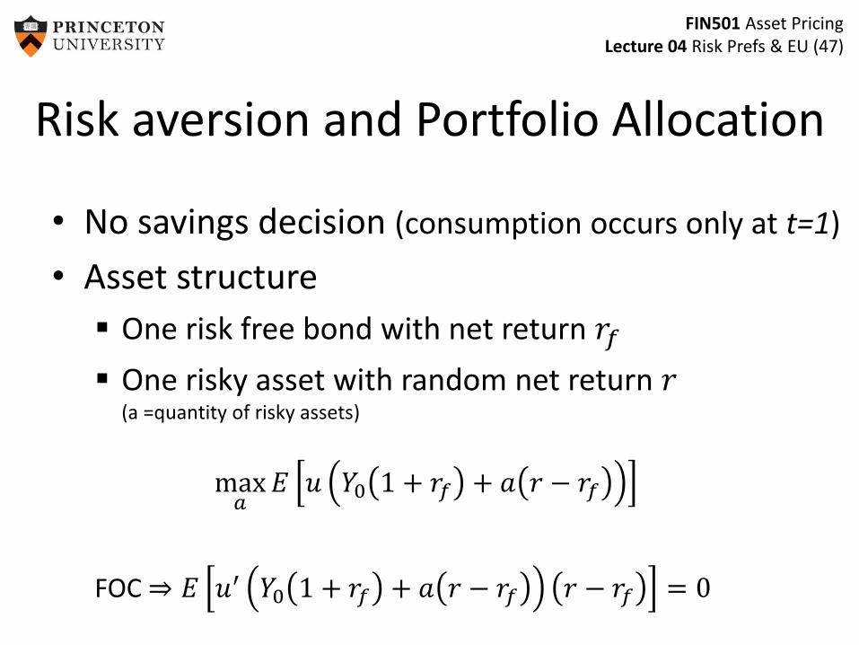
Risk aversion and Portfolio Allocation
• No savings decision (consumption occurs only at t=1)
• Asset structure
One risk free bond with net return 𝑟𝑓
One risky asset with random net return 𝑟(a =quantity of risky assets)
max𝑎
𝐸 𝑢 𝑌0 1 + 𝑟𝑓 + 𝑎 𝑟 − 𝑟𝑓
FOC ⇒ 𝐸 𝑢′ 𝑌0 1 + 𝑟𝑓 + 𝑎 𝑟 − 𝑟𝑓 𝑟 − 𝑟𝑓 = 0
FIN501 Asset PricingLecture 04 Risk Prefs & EU (48)
a
W’(a)
0
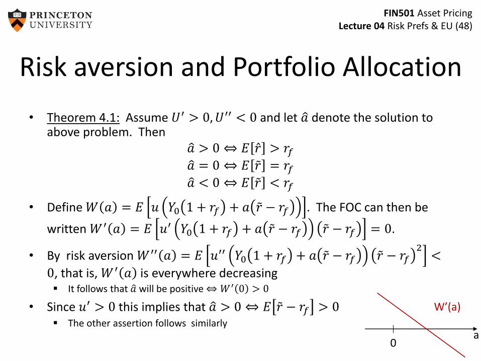
• Theorem 4.1: Assume 𝑈′ > 0,𝑈′′ < 0 and let 𝑎 denote the solution to above problem. Then
𝑎 > 0 ⇔ 𝐸 𝑟 > 𝑟𝑓 𝑎 = 0 ⇔ 𝐸 𝑟 = 𝑟𝑓 𝑎 < 0 ⇔ 𝐸 𝑟 < 𝑟𝑓
• Define 𝑊 𝑎 = 𝐸 𝑢 𝑌0 1 + 𝑟𝑓 + 𝑎 𝑟 − 𝑟𝑓 . The FOC can then be
written 𝑊′ 𝑎 = 𝐸 𝑢′ 𝑌0 1 + 𝑟𝑓 + 𝑎 𝑟 − 𝑟𝑓 𝑟 − 𝑟𝑓 = 0.
• By risk aversion 𝑊′′ 𝑎 = 𝐸 𝑢′′ 𝑌0 1 + 𝑟𝑓 + 𝑎 𝑟 − 𝑟𝑓 𝑟 − 𝑟𝑓2
<
0, that is, 𝑊′ 𝑎 is everywhere decreasing It follows that 𝑎 will be positive ⇔ 𝑊′ 0 > 0
• Since 𝑢′ > 0 this implies that 𝑎 > 0 ⇔ 𝐸 𝑟 − 𝑟𝑓 > 0 The other assertion follows similarly
Risk aversion and Portfolio Allocation
FIN501 Asset PricingLecture 04 Risk Prefs & EU (49)
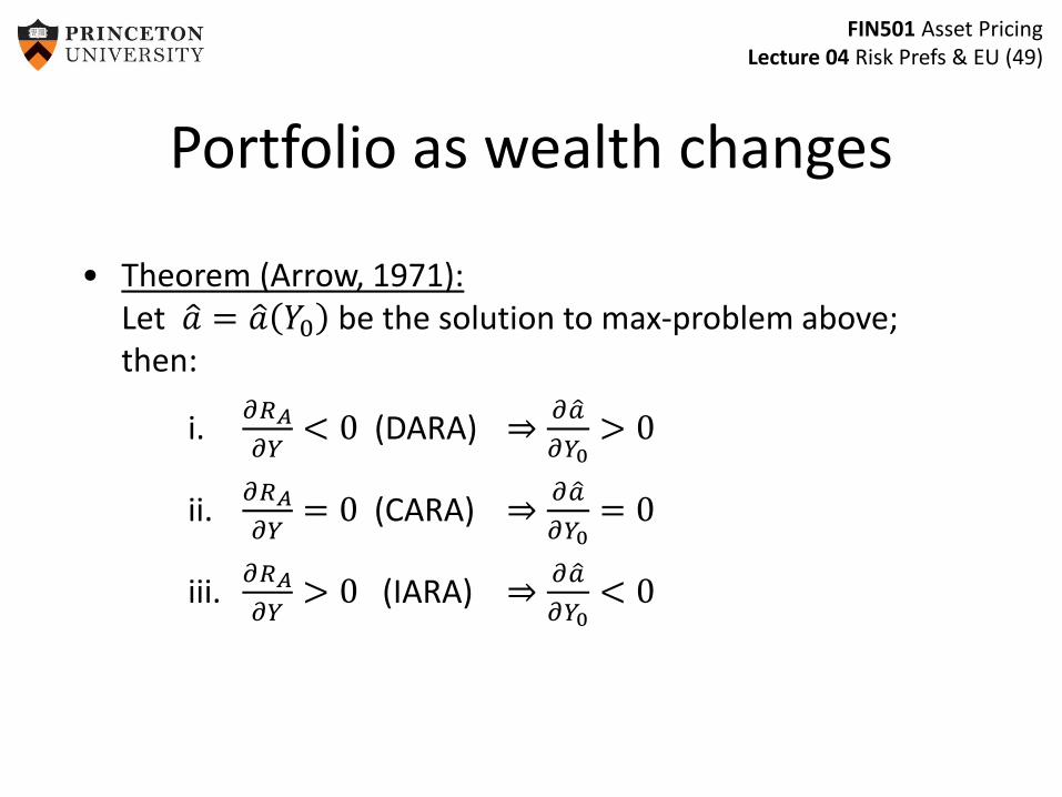
Portfolio as wealth changes
• Theorem (Arrow, 1971):Let 𝑎 = 𝑎 𝑌0 be the solution to max-problem above; then:
i.𝜕𝑅𝐴
𝜕𝑌< 0 (DARA) ⇒
𝜕 𝑎
𝜕𝑌0> 0
ii.𝜕𝑅𝐴
𝜕𝑌= 0 (CARA) ⇒
𝜕 𝑎
𝜕𝑌0= 0
iii.𝜕𝑅𝐴
𝜕𝑌> 0 (IARA) ⇒
𝜕 𝑎
𝜕𝑌0< 0
FIN501 Asset PricingLecture 04 Risk Prefs & EU (50)
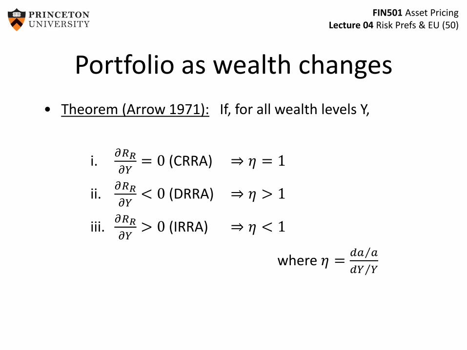
Portfolio as wealth changes
• Theorem (Arrow 1971): If, for all wealth levels Y,
i.𝜕𝑅𝑅
𝜕𝑌= 0 (CRRA) ⇒ 𝜂 = 1
ii.𝜕𝑅𝑅
𝜕𝑌< 0 (DRRA) ⇒ 𝜂 > 1
iii.𝜕𝑅𝑅
𝜕𝑌> 0 (IRRA) ⇒ 𝜂 < 1
where 𝜂 = 𝑑𝑎 𝑎
𝑑𝑌 𝑌
FIN501 Asset PricingLecture 04 Risk Prefs & EU (51)
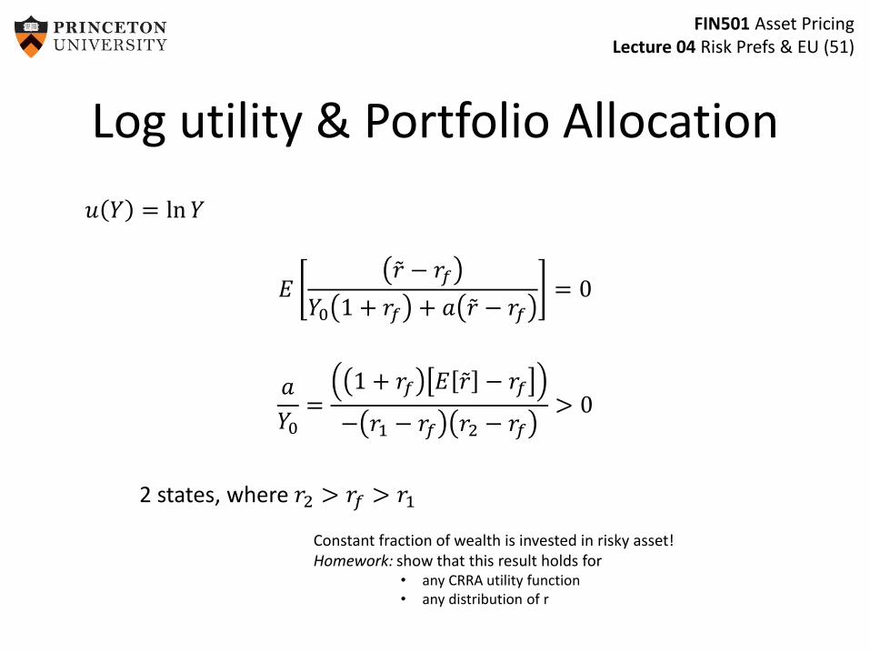
Log utility & Portfolio Allocation
𝑢 𝑌 = ln𝑌
𝐸 𝑟 − 𝑟𝑓
𝑌0 1 + 𝑟𝑓 + 𝑎 𝑟 − 𝑟𝑓= 0
𝑎
𝑌0=
1 + 𝑟𝑓 𝐸 𝑟 − 𝑟𝑓
− 𝑟1 − 𝑟𝑓 𝑟2 − 𝑟𝑓> 0
2 states, where 𝑟2 > 𝑟𝑓 > 𝑟1
Constant fraction of wealth is invested in risky asset!Homework: show that this result holds for
• any CRRA utility function• any distribution of r
FIN501 Asset PricingLecture 04 Risk Prefs & EU (52)
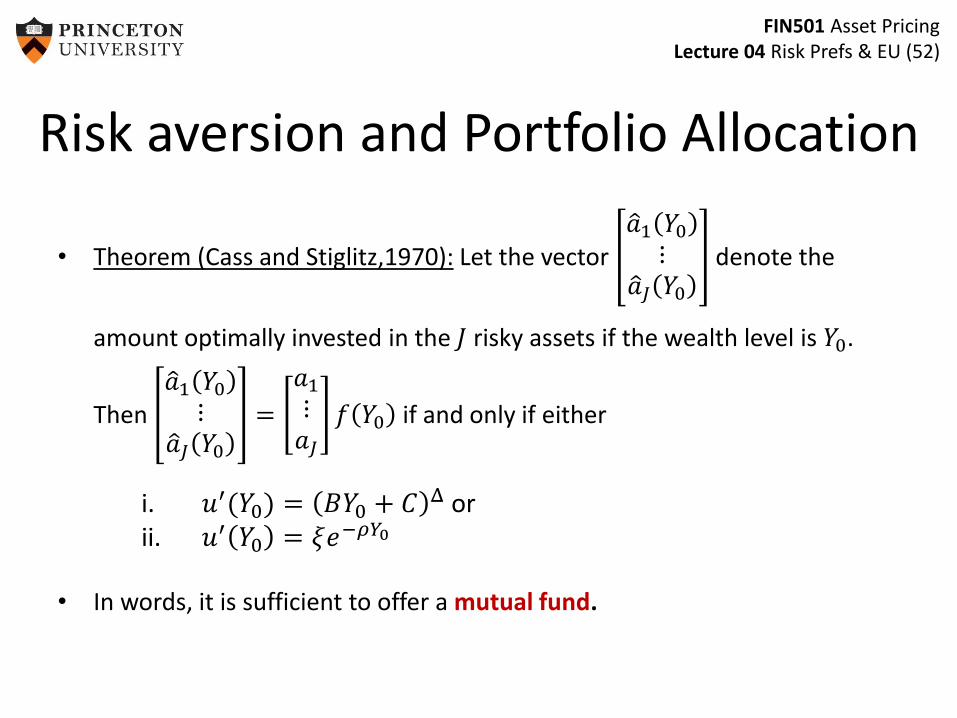
• Theorem (Cass and Stiglitz,1970): Let the vector 𝑎1 𝑌0
⋮ 𝑎𝐽 𝑌0
denote the
amount optimally invested in the 𝐽 risky assets if the wealth level is 𝑌0.
Then 𝑎1 𝑌0
⋮ 𝑎𝐽 𝑌0
=
𝑎1
⋮𝑎𝐽
𝑓 𝑌0 if and only if either
i. 𝑢′(𝑌0) = 𝐵𝑌0 + 𝐶 Δ orii. 𝑢′ 𝑌0 = 𝜉𝑒−𝜌𝑌0
• In words, it is sufficient to offer a mutual fund.
Risk aversion and Portfolio Allocation
FIN501 Asset PricingLecture 04 Risk Prefs & EU (53)
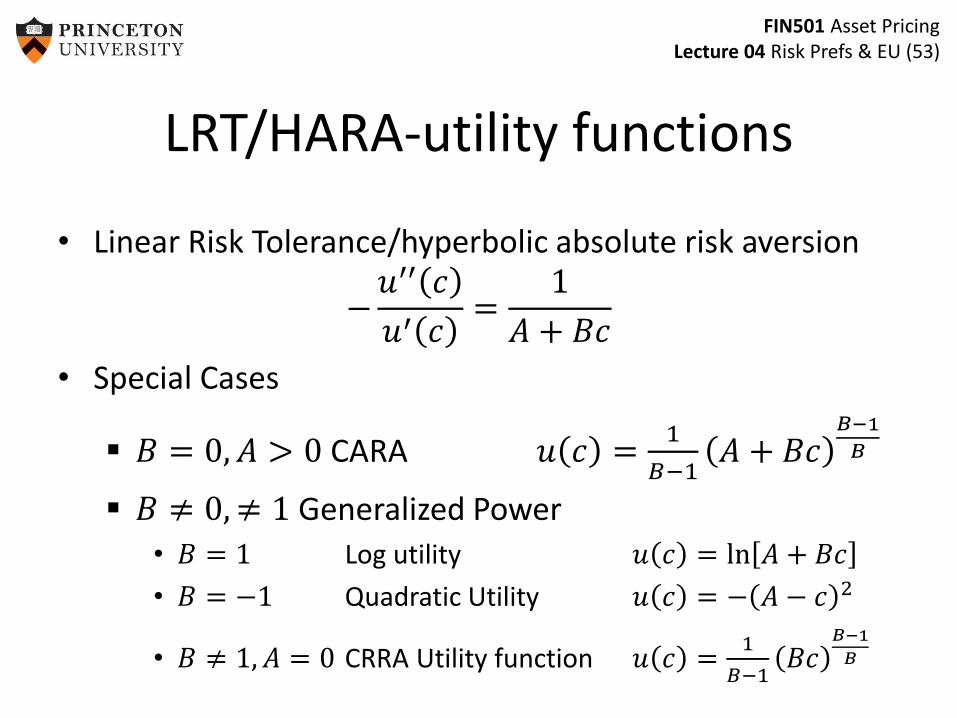
LRT/HARA-utility functions
• Linear Risk Tolerance/hyperbolic absolute risk aversion
−𝑢′′ 𝑐
𝑢′ 𝑐=
1
𝐴 + 𝐵𝑐
• Special Cases
𝐵 = 0, 𝐴 > 0 CARA 𝑢 𝑐 =1
𝐵−1𝐴 + 𝐵𝑐
𝐵−1
𝐵
𝐵 ≠ 0,≠ 1 Generalized Power
• 𝐵 = 1 Log utility 𝑢 𝑐 = ln 𝐴 + 𝐵𝑐
• 𝐵 = −1 Quadratic Utility 𝑢 𝑐 = − 𝐴 − 𝑐 2
• 𝐵 ≠ 1, 𝐴 = 0 CRRA Utility function 𝑢 𝑐 =1
𝐵−1𝐵𝑐
𝐵−1
𝐵
FIN501 Asset PricingLecture 04 Risk Prefs & EU (54)
Overview: Risk Preferences
1. State-by-state dominance
2. Stochastic dominance [DD4]
3. vNM expected utility theorya) Intuition [L4]
b) Axiomatic foundations [DD3]
4. Risk aversion coefficients and portfolio choice [DD5,L4]
5. Uncertainty/ambiguity aversion
6. Prudence coefficient and precautionary savings [DD5]
7. Mean-variance preferences [L4.6]
FIN501 Asset PricingLecture 04 Risk Prefs & EU (55)
Digression: Subjective EU Theory
• Derive perceived probability from preferences!
Set 𝑆 of prizes/consequences
Set 𝑍 of states
Set of functions 𝑓 𝑠 ∈ 𝑍, called acts (consumption plans)
• Seven SAVAGE Axioms
Goes beyond scope of this course.
FIN501 Asset PricingLecture 04 Risk Prefs & EU (56)
Digression: Ellsberg Paradox
• 10 balls in an urn Lottery 1: win $100 if you draw a red ballLottery 2: win $100 if you draw a blue ball
• Uncertainty: Probability distribution is not known
• Risk: Probability distribution is known(5 balls are red, 5 balls are blue)
• Individuals are “uncertainty/ambiguity averse”(non-additive probability approach)
FIN501 Asset PricingLecture 04 Risk Prefs & EU (57)
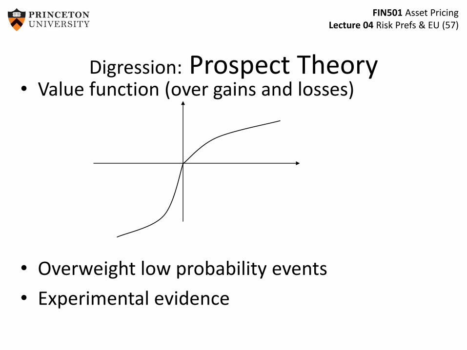
Digression: Prospect Theory• Value function (over gains and losses)
• Overweight low probability events
• Experimental evidence
FIN501 Asset PricingLecture 04 Risk Prefs & EU (58)
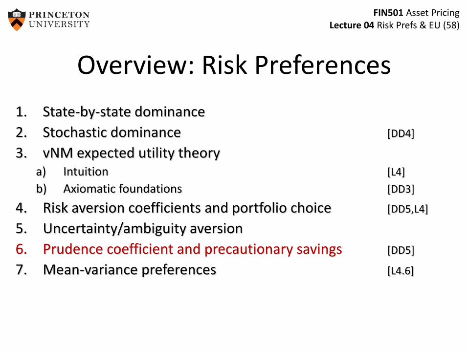
Overview: Risk Preferences
1. State-by-state dominance
2. Stochastic dominance [DD4]
3. vNM expected utility theorya) Intuition [L4]
b) Axiomatic foundations [DD3]
4. Risk aversion coefficients and portfolio choice [DD5,L4]
5. Uncertainty/ambiguity aversion
6. Prudence coefficient and precautionary savings [DD5]
7. Mean-variance preferences [L4.6]
FIN501 Asset PricingLecture 04 Risk Prefs & EU (59)
Introducing Savings
• Introduce savings decision: Consumption at 𝑡 = 0 and 𝑡 = 1
• Asset structure 1:
– risk free bond 𝑅𝑓
– NO risky asset with random return
– Increase 𝑅𝑓:– Substitution effect: shift consumption from 𝑡 = 0 to 𝑡 = 1
⇒ save more
– Income effect: agent is “effectively richer” and wants to consume some of the additional richness at 𝑡 = 0⇒ save less
– For log-utility (𝛾 = 1) both effects cancel each other
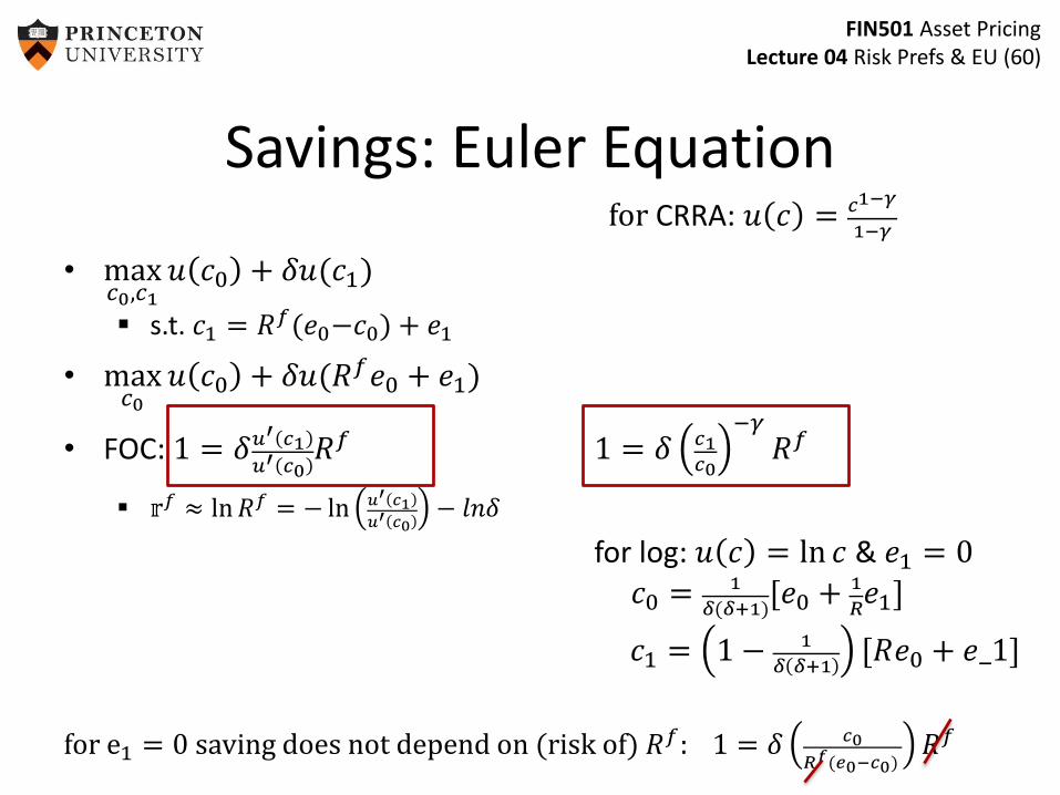
FIN501 Asset PricingLecture 04 Risk Prefs & EU (60)
Savings: Euler Equationfor CRRA: 𝑢 𝑐 = 𝑐1−𝛾
1−𝛾
• max𝑐0,𝑐1
𝑢 𝑐0 + 𝛿𝑢(𝑐1)
s.t. 𝑐1 = 𝑅𝑓(𝑒0−𝑐0) + 𝑒1
• max𝑐0
𝑢 𝑐0 + 𝛿𝑢(𝑅𝑓𝑒0 + 𝑒1)
• FOC: 1 = 𝛿𝑢′ 𝑐1𝑢′ 𝑐0
𝑅𝑓 1 = 𝛿 𝑐1𝑐0
−𝛾𝑅𝑓
𝕣𝑓 ≈ ln𝑅𝑓 = − ln 𝑢′ 𝑐1𝑢′ 𝑐0
− 𝑙𝑛𝛿
for log: 𝑢 𝑐 = ln 𝑐 & 𝑒1 = 0
𝑐0 = 1
𝛿(𝛿+1)[𝑒0 + 1
𝑅𝑒1]
𝑐1 = 1 − 1
𝛿 𝛿+1[𝑅𝑒0 + 𝑒_1]
for e1 = 0 saving does not depend on (risk of) 𝑅𝑓: 1 = 𝛿 𝑐0
𝑅𝑓(𝑒0−𝑐0)𝑅𝑓
FIN501 Asset PricingLecture 04 Risk Prefs & EU (61)
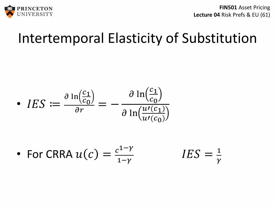
Intertemporal Elasticity of Substitution
• 𝐼𝐸𝑆 ≔𝜕 ln
𝑐1𝑐0
𝜕𝑟= −
𝜕 ln𝑐1𝑐0
𝜕 ln𝑢′(𝑐1)
𝑢′(𝑐0)
• For CRRA 𝑢 𝑐 = 𝑐1−𝛾
1−𝛾𝐼𝐸𝑆 = 1
𝛾
FIN501 Asset PricingLecture 04 Risk Prefs & EU (62)
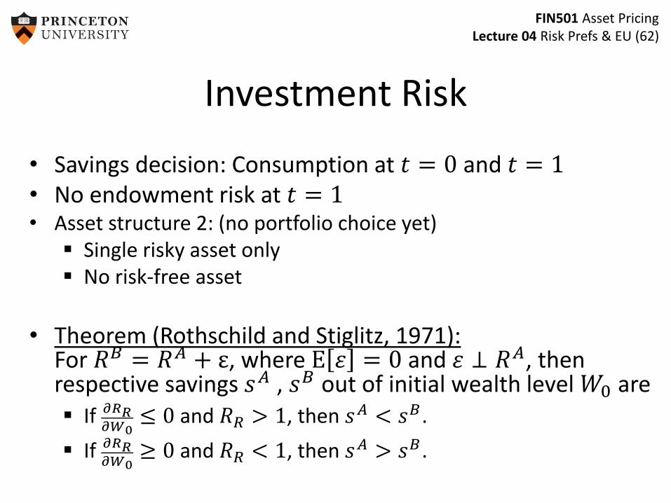
Investment Risk
• Savings decision: Consumption at 𝑡 = 0 and 𝑡 = 1• No endowment risk at 𝑡 = 1• Asset structure 2: (no portfolio choice yet)
Single risky asset only No risk-free asset
• Theorem (Rothschild and Stiglitz, 1971): For 𝑅𝐵 = 𝑅𝐴 + ε, where E 휀 = 0 and 휀 ⊥ 𝑅𝐴, then respective savings 𝑠𝐴 , 𝑠𝐵 out of initial wealth level 𝑊0 are If 𝜕𝑅𝑅
𝜕𝑊0≤ 0 and 𝑅𝑅 > 1, then 𝑠𝐴 < 𝑠𝐵.
If 𝜕𝑅𝑅𝜕𝑊0
≥ 0 and 𝑅𝑅 < 1, then 𝑠𝐴 > 𝑠𝐵.
FIN501 Asset PricingLecture 04 Risk Prefs & EU (63)
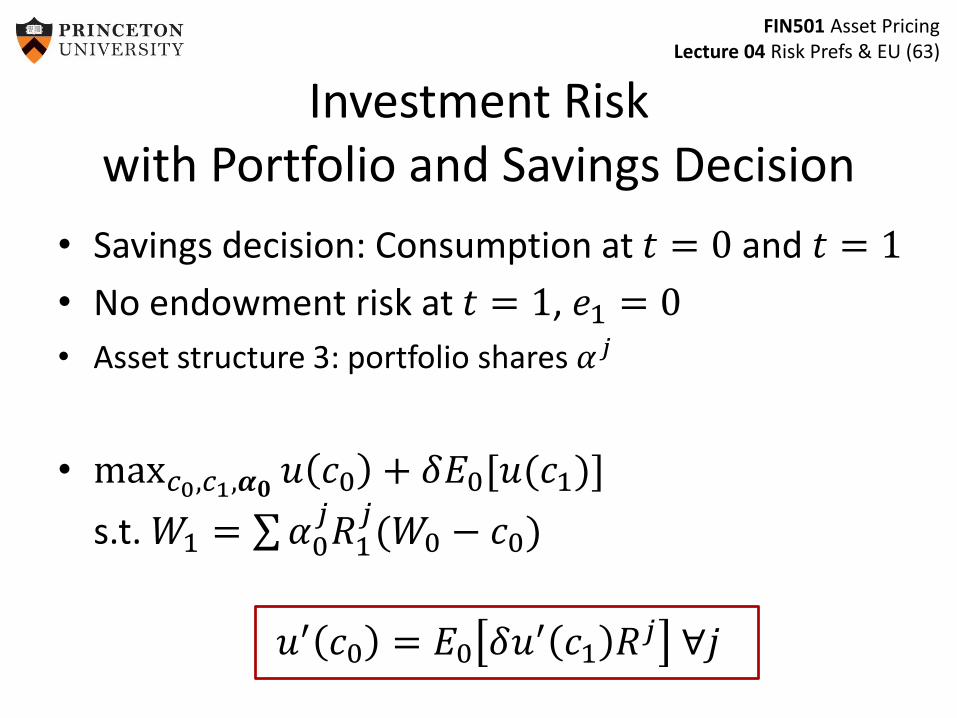
Investment Risk with Portfolio and Savings Decision
• Savings decision: Consumption at 𝑡 = 0 and 𝑡 = 1
• No endowment risk at 𝑡 = 1, 𝑒1 = 0
• Asset structure 3: portfolio shares 𝛼𝑗
• max𝑐0,𝑐1,𝜶𝟎𝑢 𝑐0 + 𝛿𝐸0[𝑢(𝑐1)]
s.t. 𝑊1 = 𝛼0𝑗𝑅1
𝑗(𝑊0 − 𝑐0)
𝑢′ 𝑐0 = 𝐸0 𝛿𝑢′ 𝑐1 𝑅𝑗 ∀𝑗
FIN501 Asset PricingLecture 04 Risk Prefs & EU (64)
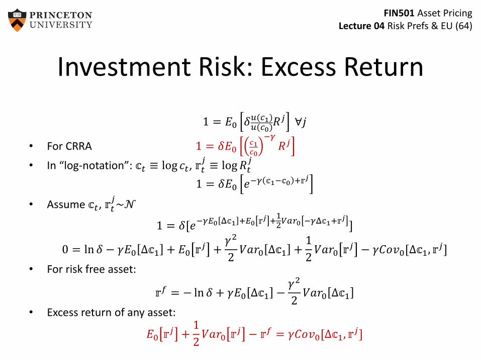
Investment Risk: Excess Return
1 = 𝐸0 𝛿𝑢(𝑐1)𝑢(𝑐0)
𝑅𝑗 ∀𝑗
• For CRRA 1 = 𝛿𝐸0𝑐1𝑐0
−𝛾𝑅𝑗
• In “log-notation”: 𝕔𝑡 ≡ log 𝑐𝑡, 𝕣𝑡𝑗≡ log𝑅𝑡
𝑗
1 = 𝛿𝐸0 𝑒−𝛾 𝕔1−𝕔0 +𝕣𝑗
• Assume 𝕔𝑡, 𝕣𝑡𝑗~𝒩
1 = 𝛿[𝑒−𝛾𝐸0 Δ𝕔1 +𝐸0 𝕣𝑗 +12𝑉𝑎𝑟0 −𝛾Δ𝕔1+𝕣𝑗 ]
0 = ln 𝛿 − 𝛾𝐸0 Δ𝕔1 + 𝐸0 𝕣𝑗 +𝛾2
2𝑉𝑎𝑟0 Δ𝕔1 +
1
2𝑉𝑎𝑟0 𝕣𝑗 − 𝛾𝐶𝑜𝑣0[Δ𝕔1, 𝕣
𝑗]
• For risk free asset:
𝕣𝑓 = − ln 𝛿 + 𝛾𝐸0 Δ𝕔1 −𝛾2
2𝑉𝑎𝑟0 Δ𝕔1
• Excess return of any asset:
𝐸0 𝕣𝑗 +1
2𝑉𝑎𝑟0 𝕣𝑗 − 𝕣𝑓 = 𝛾𝐶𝑜𝑣0[Δ𝕔1, 𝕣
𝑗]
FIN501 Asset PricingLecture 04 Risk Prefs & EU (65)
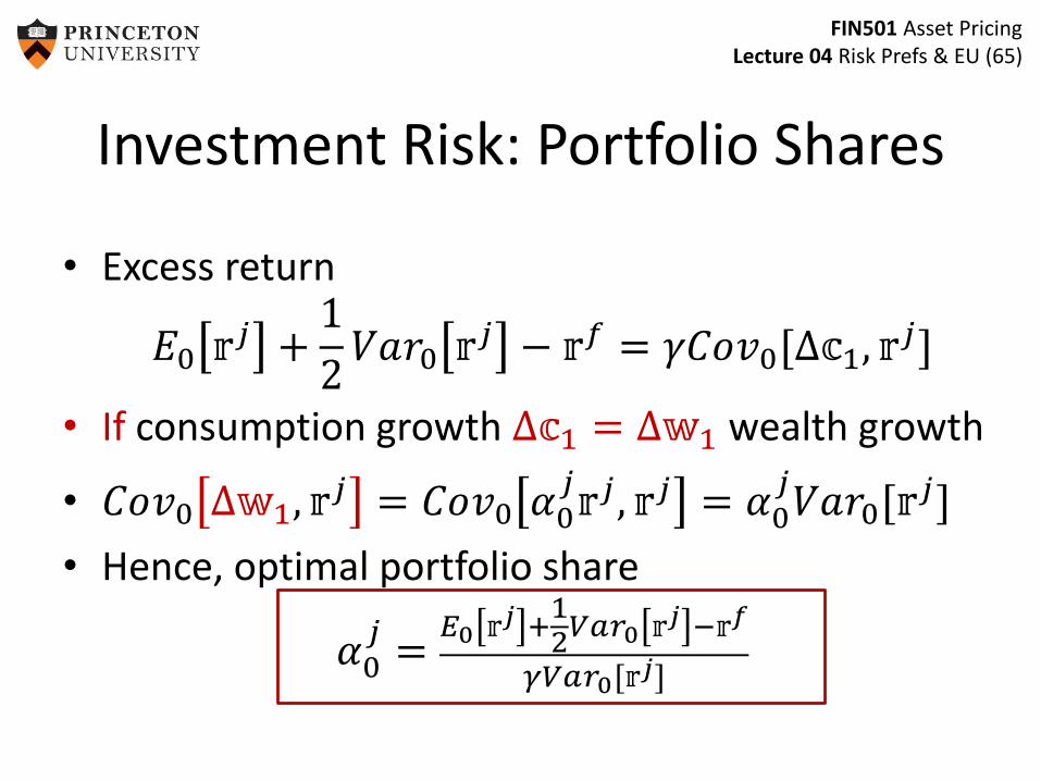
Investment Risk: Portfolio Shares
• Excess return
𝐸0 𝕣𝑗 +1
2𝑉𝑎𝑟0 𝕣𝑗 − 𝕣𝑓 = 𝛾𝐶𝑜𝑣0[Δ𝕔1, 𝕣
𝑗]
• If consumption growth Δ𝕔1 = Δ𝕨1 wealth growth
• 𝐶𝑜𝑣0 Δ𝕨1, 𝕣𝑗 = 𝐶𝑜𝑣0 𝛼0
𝑗𝕣𝑗, 𝕣𝑗 = 𝛼0
𝑗𝑉𝑎𝑟0[𝕣
𝑗]
• Hence, optimal portfolio share
𝛼0𝑗=
𝐸0 𝕣𝑗 +12𝑉𝑎𝑟0 𝕣𝑗 −𝕣𝑓
𝛾𝑉𝑎𝑟0[𝕣𝑗]
FIN501 Asset PricingLecture 04 Risk Prefs & EU (66)
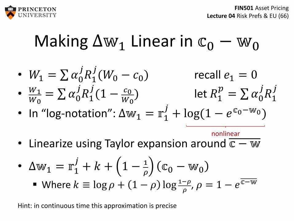
Making Δ𝕨1 Linear in 𝕔0 − 𝕨0
• 𝑊1 = 𝛼0𝑗𝑅1
𝑗(𝑊0 − 𝑐0) recall 𝑒1 = 0
• 𝑊1𝑊0
= 𝛼0𝑗𝑅1
𝑗(1 − 𝑐0
𝑊0) let 𝑅1
𝑝= 𝛼0
𝑗𝑅1
𝑗
• In “log-notation”: Δ𝕨1 = 𝕣1𝑗+ log(1 − 𝑒𝕔0−𝕨0)
• Linearize using Taylor expansion around 𝕔 − 𝕨
• Δ𝕨1 = 𝕣1𝑗+ 𝑘 + 1 − 1
𝜌𝕔0 − 𝕨0
Where 𝑘 ≡ log 𝜌 + 1 − 𝜌 log 1−𝜌
𝜌, 𝜌 = 1 − 𝑒𝕔−𝕨
Hint: in continuous time this approximation is precise
nonlinear
FIN501 Asset PricingLecture 04 Risk Prefs & EU (67)
Endowment Risk: Prudence and Pre-cautionary Savings
• Savings decisionConsumption at 𝑡 = 0 and 𝑡 = 1
• Asset structure 2: No investment risk: riskfree bond
Endowment at 𝑡 = 1 is random (background risk)
• 2 effects: Tomorrow consumption is more volatile consume more today, since it’s not risky
save more for precautionary reasons
FIN501 Asset PricingLecture 04 Risk Prefs & EU (68)
• Risk aversion is about the willingness to insure …
• … but not about its comparative statics.
• How does the behavior of an agent change when we marginally increase his exposure to risk?
• An old hypothesis (J.M. Keynes) is that people save more when they face greater uncertainty
precautionary saving
• Two forms: Shape of utility function 𝑢′′′
Borrowing constraint 𝑎𝑡 ≥ −𝑏
Prudence and Pre-cautionary Savings
FIN501 Asset PricingLecture 04 Risk Prefs & EU (69)
Precautionary Savings 1: Prudence
• Utility maximization 𝑢 𝑐0 + 𝛿𝑢𝐸0[𝑢(𝑐1)] Budget constraint: 𝑐1 = 𝑒1 + 1 + 𝑟 (𝑒0 − 𝑐0) Standard Euler equation: 𝑢′ 𝑐𝑡 = 𝛿 1 + 𝑟 𝐸𝑡 𝑢′ 𝑐𝑡+1
• If 𝑢′′′ > 0, then Jensen’s inequality implies:
•1
𝛿 1+𝑟=
𝐸𝑡 𝑢′ 𝑐𝑡+1
𝑢′ 𝑐𝑡>
𝑢′ 𝐸𝑡 𝑐𝑡+1
𝑢′ 𝑐𝑡• Increase variance of 𝑒1 (mean preserving spread)• Numerator 𝐸𝑡[𝑢
′ 𝑐𝑡+1 ] increases with variance of 𝑐𝑡+1
• For equality to hold, denominator has to increase𝑐𝑡 has to decrease, i.e. savings has to increase precautionary savings
• Prudence refers to curvature of 𝑢′, i.e. 𝑃 = −𝑢′′′
𝑢′′
FIN501 Asset PricingLecture 04 Risk Prefs & EU (70)
• Does not directly follow from risk aversion, involves 𝑢′′′ Leland (1968)
• Kimball (1990) defines absolute prudence as
𝑃 𝑐 ≔ −𝑢′′′ 𝑐
𝑢′′ 𝑐• Precautionary saving if any only if prudent.
important for comparative statics of interest rates.
• DARA ⇒ Prudence𝜕 −
𝑢′′
𝑢′
𝜕𝑐< 0, −
𝑢′′′
𝑢′′> −
𝑢′′
𝑢′
Precautionary Savings 1: Prudence
FIN501 Asset PricingLecture 04 Risk Prefs & EU (71)
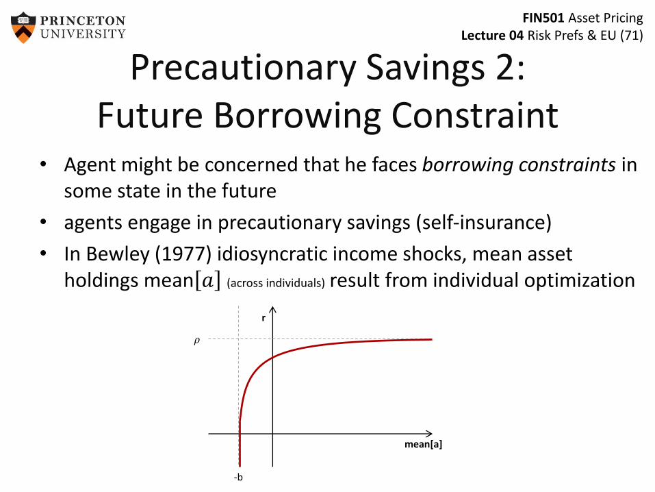
Precautionary Savings 2: Future Borrowing Constraint
• Agent might be concerned that he faces borrowing constraints in some state in the future
• agents engage in precautionary savings (self-insurance)
• In Bewley (1977) idiosyncratic income shocks, mean asset holdings mean 𝑎 (across individuals) result from individual optimization
mean[a]
-b
r
𝜌
FIN501 Asset PricingLecture 04 Risk Prefs & EU (76)
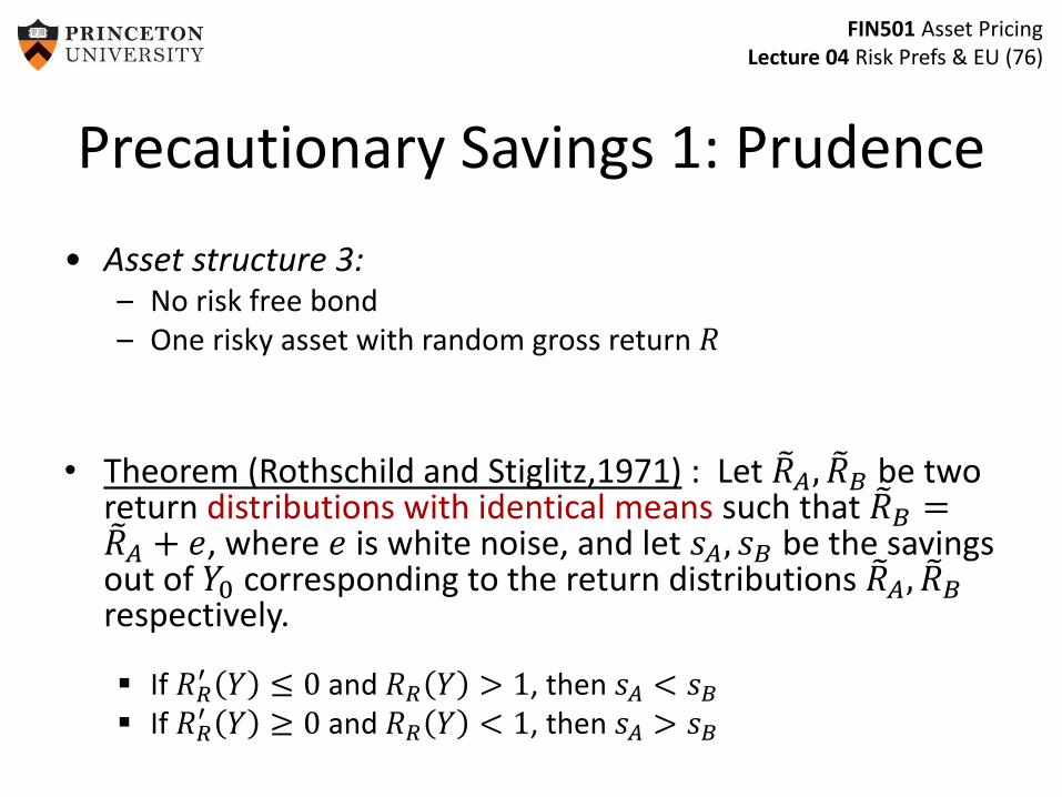
• Asset structure 3:– No risk free bond– One risky asset with random gross return 𝑅
• Theorem (Rothschild and Stiglitz,1971) : Let 𝑅𝐴, 𝑅𝐵 be two return distributions with identical means such that 𝑅𝐵 = 𝑅𝐴 + 𝑒, where 𝑒 is white noise, and let 𝑠𝐴, 𝑠𝐵 be the savings out of 𝑌0 corresponding to the return distributions 𝑅𝐴, 𝑅𝐵respectively.
If 𝑅𝑅′ 𝑌 ≤ 0 and 𝑅𝑅 𝑌 > 1, then 𝑠𝐴 < 𝑠𝐵
If 𝑅𝑅′ 𝑌 ≥ 0 and 𝑅𝑅 𝑌 < 1, then 𝑠𝐴 > 𝑠𝐵
Precautionary Savings 1: Prudence
FIN501 Asset PricingLecture 04 Risk Prefs & EU (77)
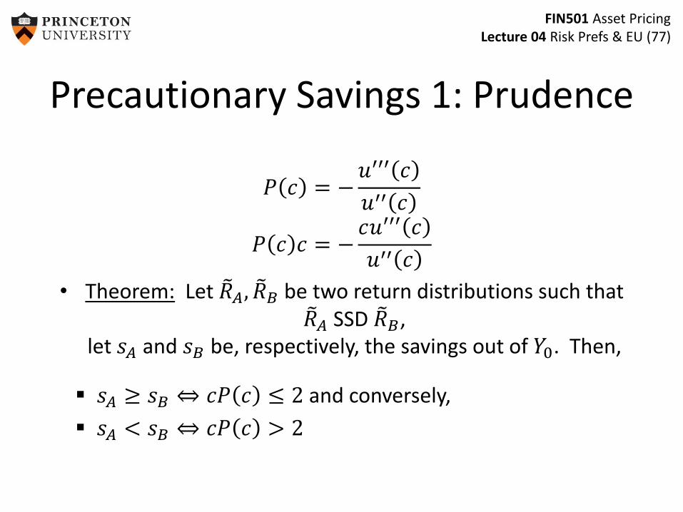
𝑃 𝑐 = −𝑢′′′ 𝑐
𝑢′′ 𝑐
𝑃 𝑐 𝑐 = −𝑐𝑢′′′ 𝑐
𝑢′′ 𝑐
• Theorem: Let 𝑅𝐴, 𝑅𝐵 be two return distributions such that 𝑅𝐴 SSD 𝑅𝐵,
let 𝑠𝐴 and 𝑠𝐵 be, respectively, the savings out of 𝑌0. Then,
𝑠𝐴 ≥ 𝑠𝐵 ⇔ 𝑐𝑃 𝑐 ≤ 2 and conversely,
𝑠𝐴 < 𝑠𝐵 ⇔ 𝑐𝑃 𝑐 > 2
Precautionary Savings 1: Prudence
FIN501 Asset PricingLecture 04 Risk Prefs & EU (78)
Overview: Risk Preferences
1. State-by-state dominance
2. Stochastic dominance [DD4]
3. vNM expected utility theorya) Intuition [L4]
b) Axiomatic foundations [DD3]
4. Risk aversion coefficients and portfolio choice [DD5,L4]
5. Uncertainty/ambiguity aversion
6. Prudence coefficient and precautionary savings [DD5]
7. Mean-variance preferences [L4.6]
FIN501 Asset PricingLecture 04 Risk Prefs & EU (79)
Mean-variance Preferences
• Early research (e.g. Markowitz and Sharpe) simply used mean and variance of return
• Mean-variance utility often easier than vNM utility function
• … but is it compatible with vNM theory?
• The answer is yes … approximately … under some conditions.
FIN501 Asset PricingLecture 04 Risk Prefs & EU (80)
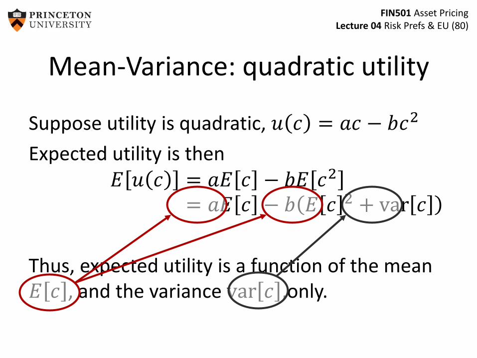
Mean-Variance: quadratic utility
Suppose utility is quadratic, 𝑢 𝑐 = 𝑎𝑐 − 𝑏𝑐2
Expected utility is then𝐸 𝑢 𝑐 = 𝑎𝐸 𝑐 − 𝑏𝐸 𝑐2
= 𝑎𝐸 𝑐 − 𝑏 𝐸 𝑐 2 + var 𝑐
Thus, expected utility is a function of the mean 𝐸 𝑐 , and the variance var 𝑐 ,only.

FIN501 Asset PricingLecture 04 Risk Prefs & EU (81)
Mean-Variance: joint normals
• Suppose all lotteries in the domain have normally distributed prized. (independence is not needed). This requires an infinite state space.
• Any linear combination of jointly normals is also normal.
• The normal distribution is completely described by its first two moments.
• Hence, expected utility can be expressed as a function of just these two numbers as well.
FIN501 Asset PricingLecture 04 Risk Prefs & EU (86)
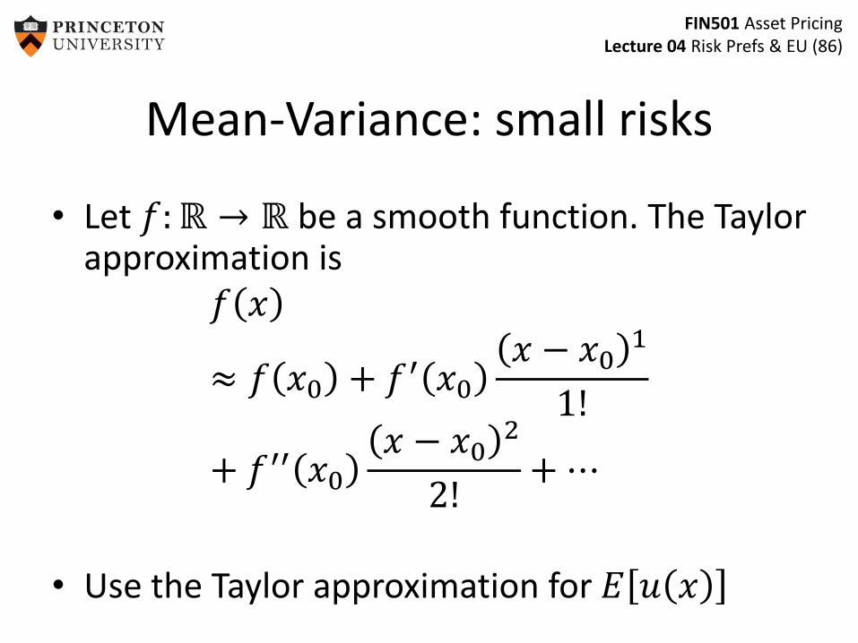
Mean-Variance: small risks
• Let 𝑓:ℝ → ℝ be a smooth function. The Taylor approximation is
𝑓 𝑥
≈ 𝑓 𝑥0 + 𝑓′ 𝑥0
𝑥 − 𝑥01
1!
+ 𝑓′′ 𝑥0
𝑥 − 𝑥02
2!+ ⋯
• Use the Taylor approximation for 𝐸 𝑢 𝑥
FIN501 Asset PricingLecture 04 Risk Prefs & EU (87)
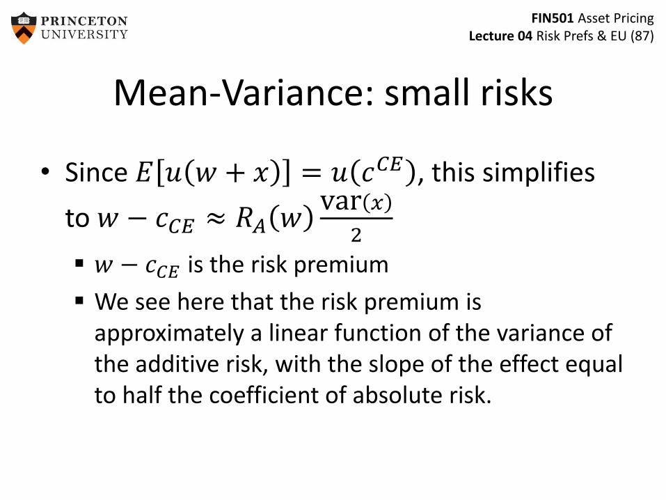
Mean-Variance: small risks
• Since 𝐸 𝑢 𝑤 + 𝑥 = 𝑢 𝑐𝐶𝐸 , this simplifies
to 𝑤 − 𝑐𝐶𝐸 ≈ 𝑅𝐴 𝑤var 𝑥
2
𝑤 − 𝑐𝐶𝐸 is the risk premium
We see here that the risk premium is approximately a linear function of the variance of the additive risk, with the slope of the effect equal to half the coefficient of absolute risk.
FIN501 Asset PricingLecture 04 Risk Prefs & EU (88)
Mean-Variance: small risks
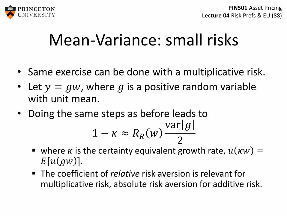
• Same exercise can be done with a multiplicative risk.
• Let 𝑦 = 𝑔𝑤, where 𝑔 is a positive random variable with unit mean.
• Doing the same steps as before leads to
1 − 𝜅 ≈ 𝑅𝑅 𝑤var 𝑔
2 where 𝜅 is the certainty equivalent growth rate, 𝑢 𝜅𝑤 =
𝐸[𝑢 𝑔𝑤 ].
The coefficient of relative risk aversion is relevant for multiplicative risk, absolute risk aversion for additive risk.