Marling and Stroud High Particle Physics Society

Data ProcessingWhat do we do with the numbers?

Pre-Calculation Considerations: Sidereal Days Earth rotates both around the sun and

its own axis.

Every day it makes one rotation around itself.

Every year it makes one revolution around the sun.

However, taking both of these into account and using the stars as reference point, the Earth appears to make one extra rotation around itself per year.

This gives the sidereal year and the celestial time system which will be used frequently for the astrophysical calculations.

Time and Angles

Our first step to locating the source of the cosmic radiation is to split the sky up into 4 quadrants (as illustrated).

Calculate the radiation from each quadrant via vector decomposition.

This requires the time to be converted to an angle (alpha), where ‘t’ is the time in solar hours and ‘T’ is the amount of hours in a sidereal day.

Using Vector Decomposition

For each time ‘t’ the data can be treated as a vector.

Alpha is the angle of the vector and the number of events is the magnitude.

This allows the data to be split into its 2 independent components using the second formula.

As each DataX and DataY can be positive or negative, the data has been split into 4 groups, for the 4 quadrants.

Summing over this data will help us detect the direction of the cosmic rays but further refinement is required…

Weighting

To analyse the data, a whole number of complete periods are required. This can be quite impractical.

To solve this we weight the data, making vales at the start and end less valuable.

The weighting function should be a pure Gauss-curve. However this curve is infinitely long therefore we will use an approximation, a raised cosine (the third formula).

To use the weighting factor, each number of coincidences (at a time ‘t’) should be multiplied by its respective weighting factor. This should be done before vector decomposition.

Weighting

Analysing the Final Data

To turn all this data into a final answer, we must take the sums of the 2 sets of data (x and y) and recompose them as vectors.

The angle between these 2 sums can be calculated using standard trigonometry.

However, this result may not be accurate, and a final formula, that compares the resultant radiation with the total radiation, can be used to find the standard deviation ( as a percentage).

AutomationIsn’t this all just a bit too tedious?

Background Info

Coded in python 2.7.9

Written using python xy in the Spyder development environment.

Compiled into a Windows .exe file using cx_freeze.

Modules used:

Tkinter and tkMessageBox

Datetime

Os and shutil

Math, numpy and pylab

Csv

urllib

The GUI Status Screen-Tells the user which files have been downloaded

Input start and end date of data collection

Input the stations that you want to get data from

Control the program from here

The Output- Folder Structure

The Output- Files

The Output- Files

Code- Constants and Setup

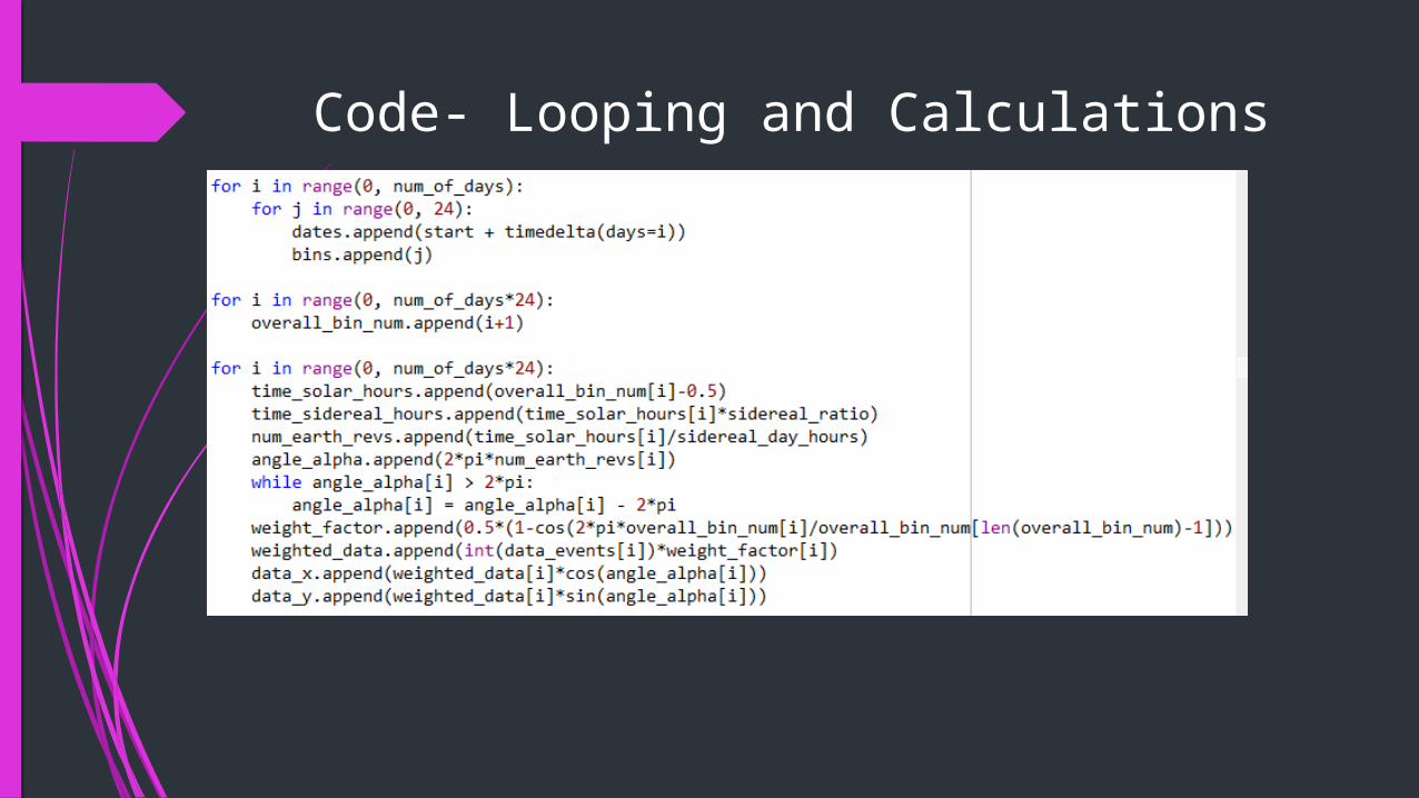
Code- Looping and Calculations

Code- Final Analysis

What's Next?

Program returns the time (or angle) at which the event took place.

This, combined with the position of the detector, can be used to find the location of the source on a star chart.

This requires additional software.

It is a manual process and it is difficult to compare star charts.

Thus a python compatible piece of virtual observatory software is required for further automation.

Our Results- Sample

There are many stations that have data for a large time span.

We shall take a sample of the stations at Eindhoven for the dates 12/01/13 to 19/01/13. All these stations were active constantly for this time period.

Station Alpha (degrees) Deviation (%)

8001 3.74356360903 3.84648164658

8002 0.0810690553796 0.845310045434

8004 21.873002378 2.08510888992

8005 14.6382874398 1.91793671168

8006 2.50822003348 13.8259604359

8007 38.7524245225 0.757092194196

8008 17.704060341 3.54404325151

8009 86.9904230463 2.55522768076

Our Results- Conclusion

All these station have similar locations.

Most have fairly low deviations and thus are quite reliable.

Expectation: similar values for alpha.

A variety of values for alpha mean we cannot pinpoint a location for the source.

Result: Inconclusive.

Cloud Chamber Workshop

Beginnings Ran a workshop for younger

students with the intention to inspire a pursuit in physics and join the PPS

Decided the subject of the workshop: detection of muons via cloud chambers, which links closely to the HiSPARC assignment

Example of a muon track

The Process

Decided to run 4 sessions due to the popularity of the workshop

Each session was run by 4 members of the HiSPARC group, with about 30 students per session

The Process Cont’d The sessions started a brief

presentation on theory and a practical demonstration on how to setup the experiment

Questionnaires assessing pupils interest in physics were handed out at the beginning and end of sessions

There was an increase of interest in taking physics further after the workshop

The Process Cont’d Students set up the apparatus

Observed cloud formation

Completed tasks during formation delays

Observed muons passing through

Dry ice was crushed, increasing surface contact area

Cern Trip Visited the LHC at Cern

Spoke to physicists about pushing the boundaries of physics

Saw the equipment used to work on the LHC and toured the LHC building

This gave us a deeper understanding of cosmic rays

Where we are now

Attaching the detector to the roof of the DT block and start analysing data

Creating a 3D model to represent the findings

Recruiting new 6th formers to help run the detector