Marriage, Social Insurance and

Labor Supply ∗

Hamish Low† Costas Meghir‡ Luigi Pistaferri§

Alessandra Voena¶

February 2016

PRELIMINARY

Abstract

This paper develops a dynamic model of marriage, labor supply, wel-fare participation, savings and divorce under limited commitment anduses it to understand the impact of welfare reforms, particularly thetime-limited eligibility, as in the TANF program. In the model, wel-fare programs can affect whether marriage and divorce take place, theextent to which people work as single or as married individuals, aswell as the allocation of resources within marriage. The model thusprovides a framework for estimating not only the short-term effects ofwelfare reforms on labor supply, but also the extent to which welfare

∗We thank participants at the CEAR Risk and Insurance workshop, the BarcelonaGSE MOVE workshop, the SED meetings, the NBER Labor Workshop and the Stanvager-Bergen Labor conference for helpful comments. Jorge Rodriguez Osorio, Samuel Seo andDavide Malacrino provided excellent research assistance.†University of Cambridge.‡Yale University, NBER and IFS.§Stanford University and NBER.¶The University of Chicago and NBER (email: avoena@uchicago.edu).

1

benefits affect family formation and the way that transfers are allo-cated within the family. This is particularly important because manyof these benefits are ultimately designed to support the well-beingof mothers and children. The limited commitment framework in ourmodel allows us to capture the effects on existing marriages as wellas marriages that will form after the reform has taken place, offeringa better understanding of transitional impacts as well as longer runeffects. Using variation provided by the introduction of time limits inwelfare benefits eligibility following the Personal Responsibility andWork Opportunity Act of 1996 (welfare reform) and data from theSurvey of Income and Program Participation between 1985 and 2011,we provide reduced form evidence of the importance of these reformson a number of outcomes relevant to our model. We then estimatethe parameters of the model using the same source of data.

2

Welfare programs are an important component of the institutional en-

vironment in most advanced economies. The structure of welfare programs

is continuously debated and often reformed as governments seek to ensure

that they achieve their insurance and redistributive function while distorting

incentives as little as possible. Our focus in this paper is a specific type of re-

form that imposes lifetime limits on welfare benefit eligibility. Understanding

the tradeoff between incentives and insurance for such programs has become

of particular importance since they were implemented in the US.

In 1996, the US implemented a major welfare reform, replacing the Aid

to Families with Dependent Children (AFDC) with the Temporary Assis-

tance for Needy Families (TANF). In the new program, the states were given

greater latitude in setting their own parameters for welfare but the length

of period over which federal government funds (in the form of block grants)

could be used to provide assistance to needy families was limited to sixty

months. States could set longer limits but would cover the financial obli-

gations with state-specific funds. About one-third of states adopted shorter

time limits. The result was that the new program varied from state to state,

with the number of years that it would be available for any one individual

being set in a decentralized way. In addition, the new program sought to

eliminate disincentives to marry or be with a partner by removing the re-

quirement of being single to be eligible for benefits, as was the case in some

states under AFDC.

In this paper, we focus on the implications of the 1996 welfare reform.

Our aim is to understand how it affected women over their life cycles in

broader terms. We start by estimating the impact of the reform on welfare

3

participation, employment, asset accumulation and marital status. To do

this, we use a difference-in-differences framework to exploit the fact that the

new welfare rules varied by state and affected different demographic groups

differently. For example, women with the youngest child close enough to 18

years old (when benefit eligibility terminates anyway) would have remained

unaffected by the time limits, while women with younger kids may be af-

fected, depending on the actions taken by their state. Within this approach

we show that welfare utilization declined quite dramatically and persistently,

employment of women increased, while the flow of both marriages and di-

vorces declined. Finally, assets increased, particularly at the lower end of the

wealth distribution.

The reduced form analysis is crucial for establishing that the reform in-

deed has important effects. However, it can neither fully reveal the dynamics

of these impacts, nor reveal the rich underlying mechanisms through which

policy changes take place. Finally, it does not offer a framework for perform-

ing counterfactual analyses, or for understanding changes in intrahousehold

distributions and welfare effects on women.

Our next step is thus to develop a life cycle model for women with endoge-

nous labor supply, marriage and savings. In this model, women are either

single or married, which is decided endogenously; children, however, arrive at

an exogenous rate estimated from the data. Marriage is characterized by lim-

ited commitment, where the outside options of both the male and the female

are key determinants of both the willingness to marry and the way resources

are allocated within the household. Depending on the circumstances, the

Pareto weight and hence the allocation of resources changes to ensure that

4

the marriage can continue (if at all possible). We model in some detail the

budget constraint facing the household, accounting for the structure of the

welfare system, including TANF and the Earned Income Tax credit (EITC).

The full structure, including the budget constraint, allows us to understand

the dynamics implied by the time limits and more generally to evaluate how

the structure of welfare affects marriage, labor supply and the allocation of

resources within the household. This latter point is important because it

allows the model to address the issue of inequality and how this is affected

by policy.

The literature on the effects of welfare reform is large and contentious.

Excellent overviews are featured in Blank (2002) and Grogger and Karoly

(2005). Experimental studies have highlighted that time limits encourage

households to limit benefits utilization to “bank” their future eligibility (Grog-

ger and Michalopoulos, 2003) and more generally are associated with reduced

utilization (Swann, 2005; Mazzolari and Ragusa, 2012).

The literature on employment effects of welfare reform has primarily fo-

cused on the sample of single women (see, for instance, Keane and Wolpin

(2010)). Recently, Chan (2013) indicates that time limits associated with

welfare reform are an important driver of the increase of labor supply in this

group. Kline and Tartari (forthcoming) examine both intensive and exten-

sive margin labor supply responses in the context of the Connecticut Jobs

First program. Limited evidence on the overall effect of welfare reform on

household formation and dissolution suggests that the reform was associated

with a small decline in divorces, while no effect has been found for transitions

into marriage (Bitler et al., 2004).

5

In addition to the above references, our paper relates to a number of dif-

ferent strands in the literature. The theoretical framework relates both to

the collective model of Chiappori (1988, 1992) and Blundell, Chiappori and

Meghir (2005) and its dynamic extension by Mazzocco (2007b), as well as its

interaction with social insurance programs (Persson, 2014). It also relates to

the life cycle analyses of female labor supply and marital status (Attanasio,

Low and Sanchez-Marcos, 2008; Fernandez and Wong, 2014), applying the

risk sharing model with limited commitment of Ligon, Thomas and Worrall

(2000) and Ligon, Thomas and Worrall (2002b), and drawing directly from

Voena (2015) by examining the implications of policy for intrahousehold al-

location in a limited commitment framework. It also contributes to existing

work on taxes and welfare in a static context include Heckman (1974), Burt-

less and Hausman (1978), Keane and Moffitt (1998), Eissa and Liebman

(1995) for the US as well as Blundell, Duncan and Meghir (1998) for the UK

and many others.

Our model is dynamic and as such it draws from the literature on dy-

namic career models such as Keane and Wolpin (1997) and subsequent models

that allow for savings and labor supply in a family context such as Blundell

et al. (2015). We build on this literature by endogenizing both marriage and

divorce and determining within the model how intrahousehold allocations

driven by the Pareto weights evolve from their initial position at the time of

marriage as the economic environment changes.

In what follows we present the data and the reduced form analysis of the

effects of the time limits component of the PROWORA. We then discuss our

model, followed by estimation, analysis of the implications and counterfactual

6

policy simulations. We end with concluding remarks.

1 The Data and Empirical Evidence on the

Effects of Time Limits

We use waves of the Survey of Income and Program Participation span-

ning the 1985-2008 period.1 We restrict the sample to individuals between 18

and 60 years old with at least one child under age 19, and who are not college

graduates. We keep only the 4th monthly observations for each individual.

Table 1 summarizes the data. Women in our sample are on average 35

years old. The program participation rate (AFDC/TANF), which is overall

7% in this population, is only 2.4% for married heads of household and

jumps to 17% for unmarried heads. There is a 1% annual divorce rate and

2% annual marriage rate. The employment rate for married and unmarried

women is about the same at 63%.

Finally, it is noteworthy that the asset holdings in this population are

not negligible, with the average being $39,000, of which $10,500 are liquid

assets. The shares of our sample with positive assets and liquid assets are

77% and 47%, respectively. Since assets are an important source of self

insurance, it is critical to take into account their presence: in the presence of

time limits, people may decide to use their own assets to smooth out large

negative income shocks, rather than exhaust their benefits eligibility upfront.

Finally, in evaluating the welfare effects of the reforms, it is important to take

1We use wave 1985, 1986, 1987, 1988, 1990, 1991, 1992, 1993, 1996, 2001, 2004 and2008.

7

Table 1: Summary statistics

Variable Obs Mean Std. Dev.age (female) 552,443 35.09 9.36assets 81,966 39,043 98,535has positive assets 81,966 0.773 0.419liquid assets 81,966 10,590 69,338has positive liquid assets 81,966 0.468 0.499employed (female) 552,443 0.632 0.482employed (female married) 355,919 0.631 0.483employed (female unmarried) 196,524 0.634 0.482program participation 486,794 0.069 0.254program participation (married head) 333,956 0.024 0.152program participation (unmarried head) 152,838 0.169 0.374divorced/separated 441,668 0.194 0.396divorced/separated (marriedt−1 = 1) 299,196 0.010 0.100married 552,443 0.644 0.479married (marriedt−1 = 0) 157,649 0.021 0.144

Notes: Data from the 1985-2011 SIPP. Sample of households in which the head is not a

college graduate and which have children below the age of 19.

precautionary savings into account.

We exploit a simple strategy to examine the relationship between the

introduction of time limits through welfare reform and our outcome variables

of interest: welfare benefits utilization, female employment, marital status

and liquid assets holdings.

1.1 Empirical strategy

The basic idea behind our descriptive empirical strategy is to compare

households that, based on their demographic characteristics and their state

of residence, could have been affected by time limits to households that were

8

not affected, before and after time limits were introduced. This strategy

extends prior work about time limits and benefits utilization (Grogger and

Michalopoulos, 2003) to cross-state variation.

We define a variable Treat which takes value 0 if the household’s expected

benefits have not changed as a result of the reform, assuming the household

has never used benefits before. Treat takes value 1 if a household’s benefits

(in terms of eligibility or amounts) have been affected in any way by the

reform. Hence, Treat is a function of the demographic characteristics of a

household and the rules of the state the household resides.

For example, if a households’s youngest child is aged 13 or above in year

t and the state’s lifetime limit is 60 months, the variable Treat takes value

0, while if a households’s youngest child is aged 12 or below in year t and the

state’s lifetime limit is 60 months, the variable Treat takes value 1.

Also, if a households’s youngest child is aged 13 in year t and the state

has an intermittent limit of 24 months every 60, the variable Treat takes

value 1. Lastly, if a households’s youngest child is aged 16 in year t and the

state’s time limit is an intermittent limit of 24 months every 60 months, the

variable Treat takes value 0, because the household would be eligible for at

most 24 months both pre- and post-reform.

The estimation equation for household i with demographics d (age of the

youngest child) in state s at time t takes the form:

yidst = αTreatdsPostst + β′Xidst + fest + feds + fes + fet + fed + εidst

where Postst equals 1 if state s has enacted the reform at time t and 0 oth-

erwise. We include state, year and demographic (age of the youngest child)

9

fixed effects, as well as state by time fixed effects to account for differen-

tial trends and state by demographic fixed effects to allow for heterogeneity

across states in the way demographic groups behave. That is, this exercise

can be seen as a difference-in-differences one that compares demographic

groups before and after welfare reform.

Figure 1 illustrates the definition of the variable Treat. The horizontal

axis represents the age of the youngest child in the household. The vertical

axis represents the number of years of potential benefits the household can

claim. The blue solid line (Pre-reform) indicates that the before the reform

the household can claim benefits for as many years as the difference between

18 and the age of the youngest child. Post-reform, Michigan maintain a

similar regime.

The variable Treat is equal to 0 whenever the line representing the regime

the household is exposed to equals the pre-reform line, and 1 otherwise.

The variable Postst is constructed based on the timing of the introduction

of time limits reported in Mazzolari and Ragusa (2012).

To study the relationship between time limits and outcome variables over

time, we allow the variable Treatds to interact differently with each calendar

year between the reform and 2011. Moreover, we estimate pre-reform inter-

actions for 1992 and 1995 to rule out pre-reform trends across demographic

groups.

yidst =2011∑

τ=1992

ατ Treatds1t = τt+β′Xidst+fest+feds+fes+fet+fed+εidst.

10

Figure 1: Time limits and the definition of treatment

Pre-reform

Michigan, post-reform

Illinois

OhioMassachussets

02

46

810

1214

1618

Year

s of

pot

entia

l sup

port

0 2 4 6 8 10 12 14 16 18Age youngest child

1.2 Results

1.2.1 Benefits utilization

We start by examining changes in the utilization of AFDC and of TANF.

On average, in our sample, 7% of households are claiming benefits (Table 1);

among households headed by an unmarried person, the rate is close to 17%.

Households that are likely to be affected by the welfare reform based on

the age of their youngest child have a 5 percentage points lower probability

11

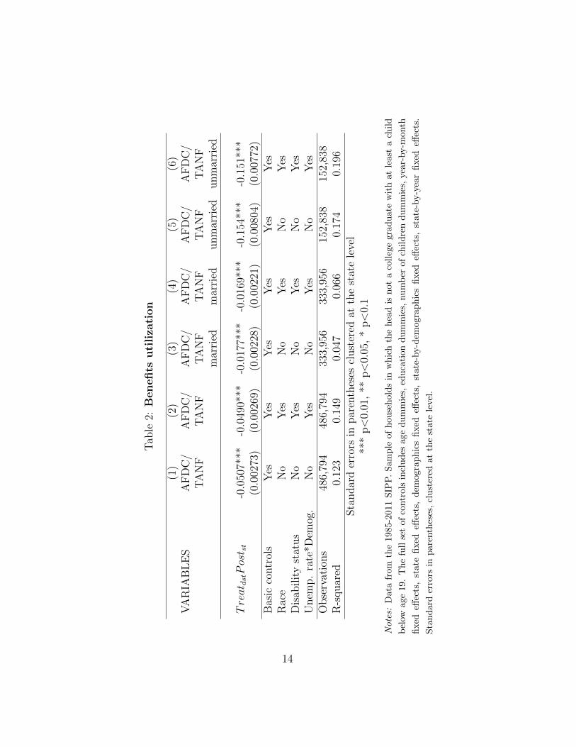
of claiming benefits after the introduction of time limits (Table 2, columns

1 and 2). Treated households headed by an unmarried person have 15 per-

centage points lower probability of claiming welfare benefits after welfare

reform, while those headed by a married head have 2 percentage points lower

probability of claiming such benefits.

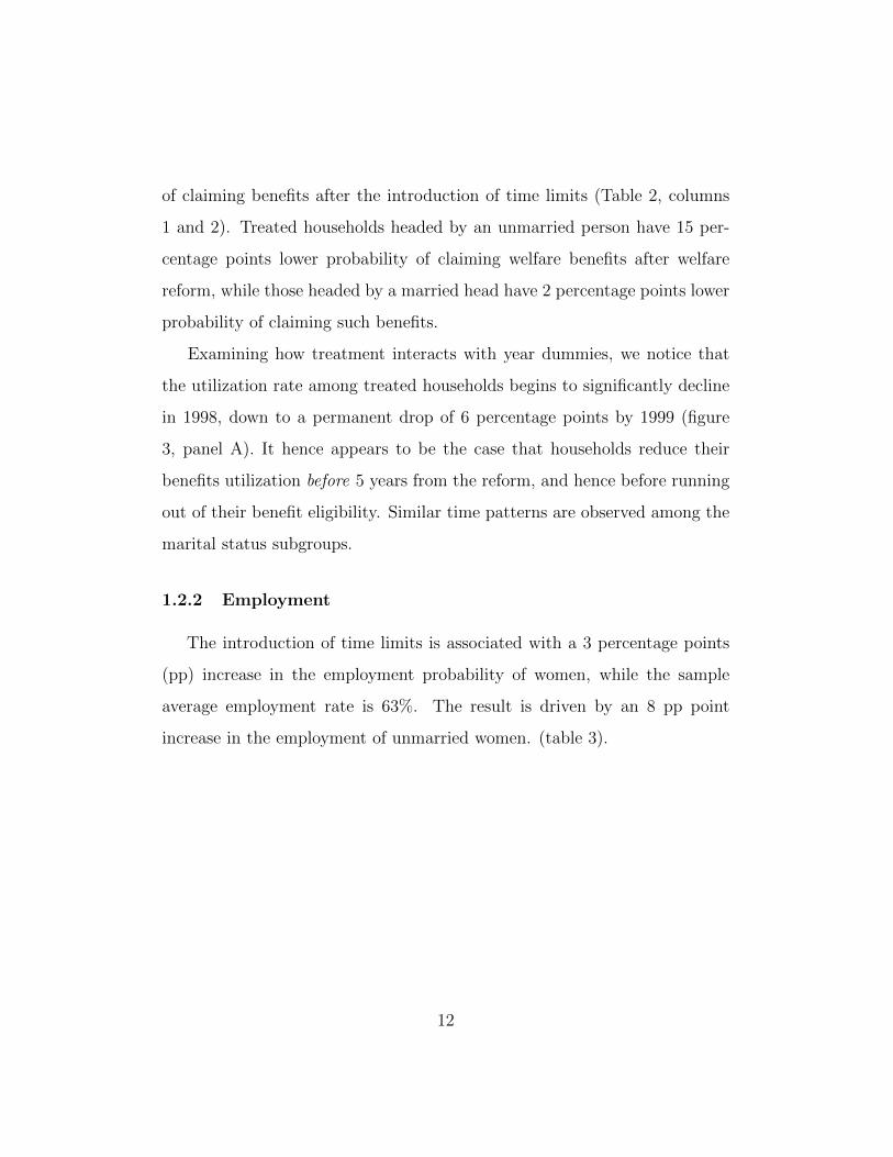
Examining how treatment interacts with year dummies, we notice that

the utilization rate among treated households begins to significantly decline

in 1998, down to a permanent drop of 6 percentage points by 1999 (figure

3, panel A). It hence appears to be the case that households reduce their

benefits utilization before 5 years from the reform, and hence before running

out of their benefit eligibility. Similar time patterns are observed among the

marital status subgroups.

1.2.2 Employment

The introduction of time limits is associated with a 3 percentage points

(pp) increase in the employment probability of women, while the sample

average employment rate is 63%. The result is driven by an 8 pp point

increase in the employment of unmarried women. (table 3).

12

Figure 2: Program participation dynamics in the short run

-.08

-.06

-.04

-.02

0.02

Coefficient

1992 1993 1994 1995 1996 1997 1998 1999 2000Year

(a) Everyone

-.2-.15

-.1-.05

0.05

Coefficient

1992 1993 1994 1995 1996 1997 1998 1999 2000Year

(b) Unmarried head

-.03

-.02

-.01

0.01

.02

Coefficient

1992 1993 1994 1995 1996 1997 1998 1999 2000Year

(c) Married head

Notes: Data from the 1990-2001 SIPP. Sample of households in which the head is not a

college graduate with at least a child below age 19. The full set of controls includes age

dummies, education dummies, number of children dummies, year-by-month fixed effects,

state fixed effects, demographics fixed effects, state-by-demographics fixed effects, state-

by-year fixed effects, race and disability status.

13

Tab

le2:

Benefits

uti

liza

tion

(1)

(2)

(3)

(4)

(5)

(6)

VA

RIA

BL

ES

AF

DC

/A

FD

C/

AF

DC

/A

FD

C/

AF

DC

/A

FD

C/

TA

NF

TA

NF

TA

NF

TA

NF

TA

NF

TA

NF

mar

ried

mar

ried

unm

arri

edunm

arri

ed

Treat dstPost st

-0.0

507*

**-0

.049

0***

-0.0

177*

**-0

.016

9***

-0.1

54**

*-0

.151

***

(0.0

0273

)(0

.002

69)

(0.0

0228

)(0

.002

21)

(0.0

0804

)(0

.007

72)

Bas

icco

ntr

ols

Yes

Yes

Yes

Yes

Yes

Yes

Rac

eN

oY

esN

oY

esN

oY

esD

isab

ilit

yst

atus

No

Yes

No

Yes

No

Yes

Unem

p.

rate

*Dem

og.

No

Yes

No

Yes

No

Yes

Obse

rvat

ions

486,

794

486,

794

333,

956

333,

956

152,

838

152,

838

R-s

quar

ed0.

123

0.14

90.

047

0.06

60.

174

0.19

6Sta

ndar

der

rors

inpar

enth

eses

clust

ered

atth

est

ate

leve

l**

*p<

0.01

,**

p<

0.05

,*

p<

0.1

Notes:

Dat

afr

omth

e19

85-2

011

SIP

P.

Sam

ple

of

hou

seh

old

sin

wh

ich

the

hea

dis

not

aco

lleg

egra

du

ate

wit

hat

least

ach

ild

bel

owag

e19

.T

he

full

set

ofco

ntr

ols

incl

ud

esag

ed

um

mie

s,ed

uca

tion

du

mm

ies,

nu

mb

erof

chil

dre

nd

um

mie

s,yea

r-by-m

onth

fixed

effec

ts,

stat

efi

xed

effec

ts,

dem

ogra

ph

ics

fixed

effec

ts,

state

-by-d

emogra

ph

ics

fixed

effec

ts,

state

-by-y

ear

fixed

effec

ts.

Sta

nd

ard

erro

rsin

par

enth

eses

,cl

ust

ered

atth

est

ate

leve

l.

14

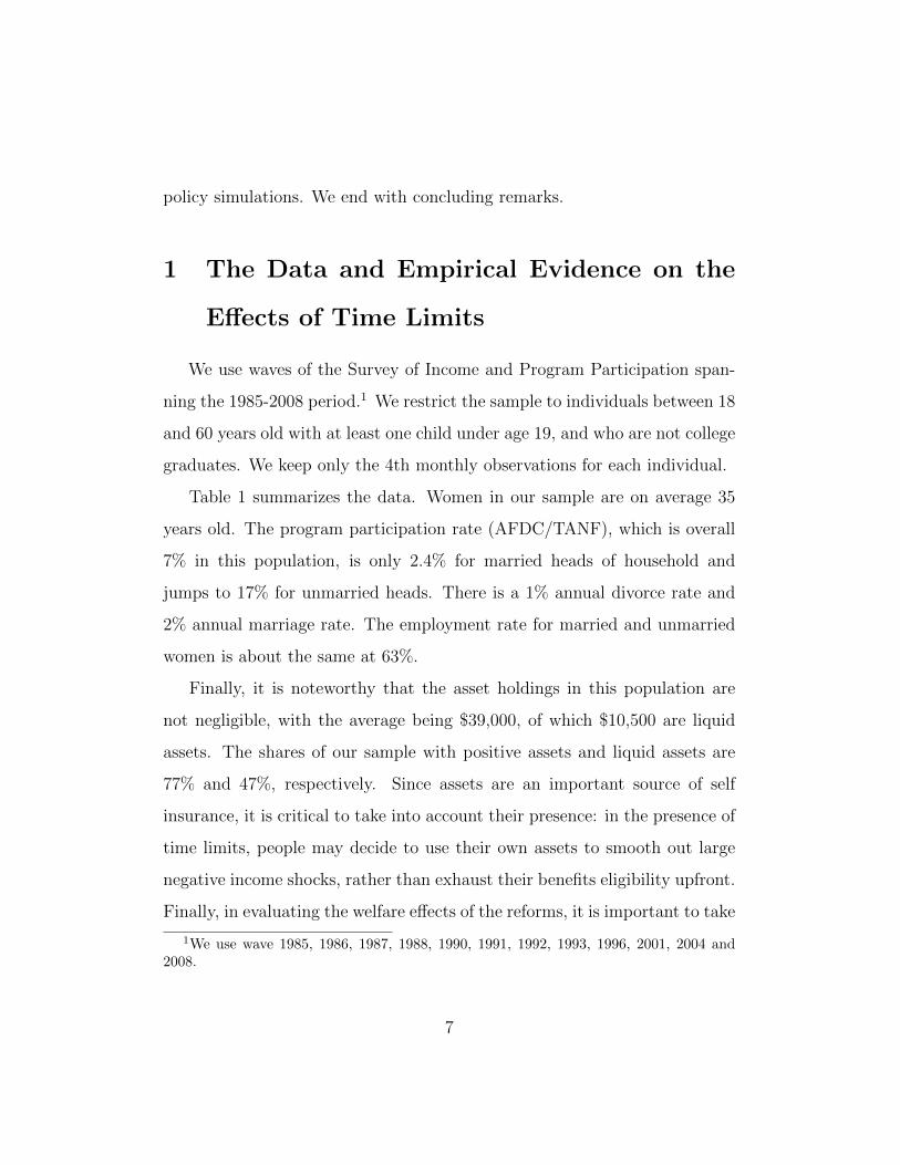
Figure 3: Program participation dynamics in the long run

-.06

-.04

-.02

0.02

.04

Coefficient

1995 2000 2005 2010Year

(a) Everyone

-.2-.15

-.1-.05

0.05

Coefficient

1995 2000 2005 2010Year

(b) Unmarried head

-.03

-.02

-.01

0.01

.02

Coefficient

1995 2000 2005 2010Year

(c) Married head

Notes: Data from the 1985-2011 SIPP. Sample of households in which the head is not a

college graduate with at least a child below age 19. The full set of controls includes age

dummies, education dummies, number of children dummies, year-by-month fixed effects,

state fixed effects, demographics fixed effects, state-by-demographics fixed effects, state-

by-year fixed effects, race and disability status.

15

Tab

le3:

Em

plo

ym

ent

statu

s-

Wom

en

(1)

(2)

(3)

(4)

(5)

(6)

VA

RIA

BL

ES

emplo

yed

emplo

yed

emplo

yed

emplo

yed

emplo

yed

emplo

yed

mar

ried

mar

ried

unm

arri

edunm

arri

ed

Treat dstPost st

0.03

17**

*0.

0294

***

-0.0

0031

1-0

.000

616

0.08

08**

*0.

0735

***

(0.0

0577

)(0

.005

44)

(0.0

0629

)(0

.006

29)

(0.0

0973

)(0

.009

97)

Bas

icco

ntr

ols

Yes

Yes

Yes

Yes

Yes

Yes

Rac

eN

oY

esN

oY

esN

oY

esD

isab

ilit

yst

atus

No

Yes

No

Yes

No

Yes

Unem

p.

rate

*Dem

og.

No

Yes

No

Yes

No

Yes

Obse

rvat

ions

552,

443

552,

443

355,

919

355,

919

196,

524

196,

524

R-s

quar

ed0.

057

0.09

80.

054

0.08

00.

082

0.16

5Sta

ndar

der

rors

inpar

enth

eses

clust

ered

atth

est

ate

leve

l**

*p<

0.01

,**

p<

0.05

,*

p<

0.1

Notes:

Dat

afr

omth

e19

85-2

011

SIP

P.

Sam

ple

of

non

-coll

ege

gra

du

ate

sw

ith

at

least

ach

ild

bel

owage

19.

Th

efu

llse

tof

contr

ols

incl

ud

esag

ed

um

mie

s,ed

uca

tion

du

mm

ies,

nu

mb

erofch

ild

ren

du

mm

ies,

year-

by-m

onth

fixed

effec

ts,st

ate

fixed

effec

ts,

dem

ogra

ph

ics

fixed

effec

ts,

stat

e-by-d

emog

rap

hic

sfi

xed

effec

ts,

state

-by-y

ear

fixed

effec

ts.

Sta

nd

ard

erro

rsin

pare

nth

eses

,

clu

ster

edat

the

stat

ele

vel

.

16

Figure 4: Employment probability dynamics in the short run-.02

0.02

.04

.06

.08

Coefficient

1992 1993 1994 1995 1996 1997 1998 1999 2000Year

(a) All women

-.05

0.05

.1.15

Coefficient

1992 1993 1994 1995 1996 1997 1998 1999 2000Year

(b) Unmarried women

-.05

0.05

.1Coefficient

1992 1993 1994 1995 1996 1997 1998 1999 2000Year

(c) Married women

Notes: Data from the 1990-2001 SIPP. Sample of non-college graduates with at least a child

below age 19. The full set of controls includes age dummies, education dummies, number

of children dummies, year-by-month fixed effects, state fixed effects, demographics fixed

effects, state-by-demographics fixed effects, state-by-year fixed effects, race and disability

status.

17

Figure 5: Employment probability dynamics in the long run-.05

0.05

.1Coefficient

1995 2000 2005 2010Year

(a) All women

-.05

0.05

.1.15

Coefficient

1995 2000 2005 2010Year

(b) Unmarried women

-.06

-.04

-.02

0.02

.04

Coefficient

1995 2000 2005 2010Year

(c) Married women

Notes: Data from the 1985-2011 SIPP. Sample of non-college graduates with at least a child

below age 19. The full set of controls includes age dummies, education dummies, number

of children dummies, year-by-month fixed effects, state fixed effects, demographics fixed

effects, state-by-demographics fixed effects, state-by-year fixed effects, race and disability

status.

1.2.3 Household formation and dissolution

A central motivation for welfare reform was to encourage marriage. In

studying this relationship, we first consider the impact of welfare reform on

the probability of being divorced or separated for women. Treated women

18

are 3 percentage points less likely to be divorced after the introduction of

time limits (table 4, columns 1 and 2). The decline is associated with a

0.2 percentage points decline in the probability of transitioning into divorce

conditional on being married during the previous interview (Table 4, columns

3 and 4).

Table 4: Divorce

(1) (2) (3) (4)VARIABLES divorce/ divorce/ divorce/ divorce/

separation separation separation separationTreatdstPostst -0.0289*** -0.0279*** -0.00170** -0.00177**

(0.00545) (0.00518) (0.000709) (0.000715)Basic controls Yes Yes Yes YesRace No Yes No YesDisability status No Yes No YesUnemp. rate*Demog. No Yes No YesConditional onmarriedt−1 = 0 No No Yes YesObservations 552,443 552,443 299,540 299,540R-squared 0.022 0.030 0.007 0.008

Standard errors in parentheses clustered at the state level*** p<0.01, ** p<0.05, * p<0.1

Notes: Data from the 1985-2011 SIPP. Sample of non-college graduate women with at

least a child below age 19. The full set of controls includes age dummies, education

dummies, number of children dummies, year-by-month fixed effects, state fixed effects,

demographics fixed effects, state-by-demographics fixed effects, state-by-year fixed effects.

Robust standard errors in parentheses.

As shown in the first two columns of Table 5, there was also a 2 percentage

points decline in the proportion married, related to a 0.3-0.4 pp point decline

in those getting married each year as shown in the last two columnes of the

same table.

19

Thus there seem to be more people staying together but at the same time

fewer are getting married as a result of the reform.

Table 5: Marriage

(1) (2) (3) (4)VARIABLES married married married married

TreatdstPostst -0.0217*** -0.0251*** -0.00308* -0.00406**(0.00772) (0.00714) (0.00171) (0.00175)

Basic controls Yes Yes Yes YesRace No Yes No YesDisability status No Yes No YesUnemp. rate*Demog. No No Yes YesConditional onmarriedt−1 = 0 No No Yes YesObservations 552,443 552,443 157,649 157,649R-squared 0.157 0.212 0.013 0.016

Standard errors in parentheses clustered at the state level*** p<0.01, ** p<0.05, * p<0.1

Notes: Data from the 1985-2011 SIPP. Sample of non-college graduate women with at

least a child below age 19. The full set of controls includes age dummies, education

dummies, number of children dummies, year-by-month fixed effects, state fixed effects,

demographics fixed effects, state-by-demographics fixed effects, state-by-year fixed effects.

Robust standard errors in parentheses.

1.2.4 Assets holdings

Overall assets show a decline which is not significant. However, when we split

the sample into those married and those not we find a decline in asset holdings

among those married, while unmarried women increase their asset holdings.

Both effects are highly significant and even with a Bonferroni adjustment,

they have a joint p-value of at most 2%. The result on single women has a

20

straightforward interpretation: the reduction in publicly provided insurance

is replaced with increased savings, as self-insurance. The married couple

effect is interesting: married couples find it harder to claim benefits, so they

probably do not lose much by the reform. Moreover, the reform induced a

decline in the divorce probability, leading to a lower demand for insurance.

Importantly, there may be important selection out of marriage for poorer

household, because of the changes in marital status documented above. It

is these complex effects that the structural model we develop will seek to

match and interpret.

The response of liquid assets holdings is similar to that of overall as-

sets. We observe a small increase in the probability of owning positive assets

around the $2,000 eligibility threshold (table 8).

21

Tab

le6:

Ass

ets

hold

ings

(1)

(2)

(3)

(4)

(5)

(6)

VA

RIA

BL

ES

asse

tsas

sets

asse

tsas

sets

asse

tsas

sets

mar

ried

mar

ried

unm

arri

edunm

arri

ed

Treat dstPost st

-3,1

13-4

,006

*-9

,831

***

-10,

595*

**5,

599*

**4,

948*

*(2

,206

)(2

,228

)(3

,361

)(3

,502

)(1

,991

)(1

,967

)B

asic

contr

ols

Yes

Yes

Yes

Yes

Yes

Yes

Rac

eN

oY

esN

oY

esN

oY

esD

isab

ilit

yst

atus

No

Yes

No

Yes

No

Yes

Unem

p.

rate

*Dem

og.

No

Yes

No

Yes

No

Yes

Obse

rvat

ions

81,9

6681

,966

55,7

3955

,739

26,2

2726

,227

R-s

quar

ed0.

061

0.07

50.

063

0.07

40.

063

0.07

5Sta

ndar

der

rors

inpar

enth

eses

clust

ered

atth

est

ate

leve

l**

*p<

0.01

,**

p<

0.05

,*

p<

0.1

par

Notes:

Dat

afr

omth

e19

85-2

011

SIP

P.

Sam

ple

of

non

-coll

ege

gra

du

ate

wom

enw

ith

at

least

ach

ild

bel

owage

19.

Th

efu

ll

set

ofco

ntr

ols

incl

ud

esag

ed

um

mie

s,ed

uca

tion

du

mm

ies,

nu

mb

erof

chil

dre

nd

um

mie

s,ye

ar-

by-m

onth

fixed

effec

ts,

state

fixed

effec

ts,

dem

ogra

ph

ics

fixed

effec

ts,

stat

e-by-d

emogra

ph

ics

fixed

effec

ts,

state

-by-y

ear

fixed

effec

ts.

Rob

ust

stand

ard

erro

rsin

par

enth

eses

.

22

Tab

le7:

Liq

uid

ass

ets

hold

ings

(1)

(2)

(3)

(4)

(5)

(6)

VA

RIA

BL

ES

liquid

liquid

liquid

liquid

liquid

liquid

wea

lth

wea

lth

wea

lth

wea

lth

wea

lth

wea

lth

mar

ried

mar

ried

unm

arri

edunm

arri

ed

Treat dstPost st

-2,9

60*

-3,3

68*

-6,6

89**

*-7

,032

***

2,38

22,

151

(1,6

12)

(1,7

56)

(2,2

67)

(2,4

38)

(1,5

14)

(1,5

40)

Bas

icco

ntr

ols

Yes

Yes

Yes

Yes

Yes

Yes

Rac

eN

oY

esN

oY

esN

oY

esD

isab

ilit

yst

atus

No

Yes

No

Yes

No

Yes

Unem

p.

rate

*Dem

og.

No

Yes

No

Yes

No

Yes

Obse

rvat

ions

81,9

6681

,966

55,7

3955

,739

26,2

2726

,227

R-s

quar

ed0.

020

0.02

50.

026

0.03

00.

030

0.03

3Sta

ndar

der

rors

inpar

enth

eses

clust

ered

atth

est

ate

leve

l**

*p<

0.01

,**

p<

0.05

,*

p<

0.1

par

Notes:

Dat

afr

omth

e19

85-2

011

SIP

P.

Sam

ple

of

non

-coll

ege

gra

du

ate

wom

enw

ith

at

least

ach

ild

bel

owage

19.

Th

efu

ll

set

ofco

ntr

ols

incl

ud

esag

ed

um

mie

s,ed

uca

tion

du

mm

ies,

nu

mb

erof

chil

dre

nd

um

mie

s,ye

ar-

by-m

onth

fixed

effec

ts,

state

fixed

effec

ts,

dem

ogra

ph

ics

fixed

effec

ts,

stat

e-by-d

emogra

ph

ics

fixed

effec

ts,

state

-by-y

ear

fixed

effec

ts.

Rob

ust

stand

ard

erro

rsin

par

enth

eses

.

23

Tab

le8:

Dis

trib

uti

on

of

liquid

ass

ets

hold

ings

(1)

(2)

(3)

(4)

(5)

(6)

(7)

VA

RIA

BL

ES

P(A

t≥

0)P

(At≥

1k)

P(A

t≥

2k)

P(A

t≥

3k)

P(A

t≥

4k)

P(A

t≥

5k)

P(A

t≥

6k)

Treat dstPost st

0.01

49*

0.02

25**

*0.

0167

**0.

0099

0.00

207.

97e-

05-0

.002

8(0

.008

5)(0

.008

2)(0

.008

0)(0

.007

8)(0

.007

3)(0

.007

4)(0

.006

9)

Bas

icco

ntr

ols

Yes

Yes

Yes

Yes

Yes

Yes

Yes

Rac

eY

esY

esY

esY

esY

esY

esY

esD

isab

ilit

yst

atus

Yes

Yes

Yes

Yes

Yes

Yes

Yes

Unem

p.

rate

*Dem

og.

Yes

Yes

Yes

Yes

Yes

Yes

Yes

Obse

rvat

ions

81,9

6681

,966

81,9

6681

,966

81,9

6681

,966

81,9

66R

-squar

ed0.

026

0.11

50.

112

0.10

60.

105

0.10

30.

099

Rob

ust

stan

dar

der

rors

inpar

enth

eses

***

p<

0.01

,**

p<

0.05

,*

p<

0.1

Notes:

Dat

afr

omth

e19

85-2

011

SIP

P.

Sam

ple

ofn

on

-coll

ege

gra

du

ate

wom

enw

ith

at

least

ach

ild

bel

owage

19.

Th

efu

llse

t

ofco

ntr

ols

incl

ud

esag

ed

um

mie

s,ed

uca

tion

du

mm

ies,

nu

mb

erof

chil

dre

nd

um

mie

s,yea

r-by-m

onth

fixed

effec

ts,

state

fixed

effec

ts,

dem

ogra

ph

ics

fixed

effec

ts,

stat

e-by-d

emogra

ph

ics

fixed

effec

ts,

state

-by-y

ear

fixed

effec

ts.

Rob

ust

stand

ard

erro

rsin

par

enth

eses

.

24

1.3 Robustness checks

1.3.1 Attrition in the SIPP sample

To address concerns regarding the high rate of attrition in the SIPP

(Zabel, 1998), we limit our analysis to the first two waves for each SIPP

panel. In Appendix table 13 we show that this adjustment leaves the results

unaffected.

1.3.2 Exclude young children

A potential concern is that our results are driven by changes in the be-

havior of households with small children after welfare reform as a result of

the childcare provisions in the PRWORA. Appendix table 14 shows that the

results are robust to excluding households in which the youngest child is

below the age of 6.

2 The model

The model, while taking into account the entire family structure, focuses

primarily on the behavior of mothers, who can be single or married. Marriage

and divorce are endogenous and take place at the start of the period. We

begin by describing labor supply, savings and welfare participation choices

that take place after the marital status decision. We then describe how

marital status choices are made.

25

2.1 Problem of the single woman

We start by describing the problem of a single woman who has completed

schooling. 2 In each period, she decides whether to work, whether to claim

welfare and how much to save.

The vector of choice variables qt = cWt , PWt , Bt includes: how much

to consume (cWt ), whether she works (PWt ), and whether to claim welfare

benefits bt (Bt ∈ 0, 1) which depend on children and their age, income,

assets and past utilization. In addition, she makes a choice to marry, which

will depend on meeting a man and whether he will accept. The decision to

marry takes place at the start of the period, before any consumption or work

plan is implemented: the latter will be conditional on the marriage decision.

If she remains single, her budget constraint is given by

AWt+1

1 + r= AWt −

cWte(kat )

+ (wWt − CCat )PW

t +Btbt + FSt + EITCt (1)

AWt+1 ≥ 0

where e(kat ) is the equivalence scale due to the presence of children and CCat

is the financial cost of childcare paid if the woman works. Her wage wt is

drawn from a distribution that depends on her age and the previous period

wage.

The state space for a single woman is ΩWst = At, wt, kat , TBt, where

TBt is the number of time periods the woman has claimed the time limited

2Our main focus in on low-education women, because we are interested in the impactsof means-tested welfare benefits, such as TANF. An important question is how educationchoice is itself affected by the presence of such benefits (Blundell et al., 2015). We leavethis question for further research. ? studies women’s education decisions in a dynamiccollective model of the household with limited commitment.

26

benefit. The within-period preferences for a single woman are denoted by

uWs(cWt , PWt , Bt). We model three social programs: food stamps, EITC and

AFDC or TANF. The first two are represented by FSt and EITCt respec-

tively, while AFDC or TANF by bt. Food stamps and EITC are functions

of the vector kat , wWt PWt , At, TBt, while AFDC/TANF is a function of the

vector kat , wWt PWt , At, TBt. We discuss the parametrization of the various

benefits programs, which interact in a complex way with one another, in the

structural estimation section.

With probability λt, at the begining of the period the woman meets a man

with characteristics Am, ymt (assets and exogenous earning) and together

they draw an initial match quality s0t . In that case, they decide whether to

get married, as described below. Denote the distribution of available men

in period t as G(A, y|t). We restrict encounters to be between a man and a

woman of the same age group.3

We denote by V Wst (ΩWs

t ) the value function for a single woman at age t

and V Wmt (ΩWm

t ) the value function for a married woman at age t, which we

will define below.

A single woman has the following value functions:

V Wst (ΩWs

t ) = maxqtuWs(cWt , P

Wt , Bt)

+βEt[λt+1[(1−Mt+1(Ωt+1))V

Wst+1 (ΩWs

t+1) +Mt+1(Ωt+1)VWmt+1 (ΩM

t+1)] + (1− λt+1)VWst+1 (ΩWs

t+1)]

3In principle, this distribution is endogenous and as economic conditions change, theassociated marriage market will change, with this “offer” distribution changing. In thispaper we take this distribution as given and do not solve for it endogenously. This mainlyaffects counterfactual simulations. Note that solving for the equilibrium distribution intwo dimensions is likely to be very complicated computationally.

27

subject to the two constraints in (1).

2.2 Problem of the single man

Men solve an analogous problem without welfare benefits and without a

labor supply choice. Men’s earnings follow a stochastic process described by

the distribution fM(yMt |yMt−1, age). Children affect the man’s problem only

when he is married to their mother.

These assumptions determine V Ms(ΩMst ), the man’s value function when

he is single. V Mmt (ΩM

t ) the value accruing to a married man. In all cases Ωjt

is the relevant state space.

His budget constraint is given by

AMt+1

1 + r= AMt − cMt + yMt + FSt (2)

AMt+1 ≥ 0.

The problem for the single male is thus defined by

V Mst (ΩMs

t ) = maxcMtuMs(cMt ) + βEt[λt+1[(1−Mt+1(Ωt+1))V

Mst+1 (ΩMs

t+1)

+Mt+1(Ωt+1)VMmt+1 (ΩM

t+1)] + (1− λt+1)VMst+1 (ΩMs

t+1)].

The problem is more complex than the simple consumption smoothing and

precautionary savings problem because assets affect the probability of mar-

riage as well as the share of consumption when married.

28

2.3 Problem of the couple

The state variables, summarized in Ωmt , are: assets, spouses’ productivity,

number of periods of welfare benefits utilization, age of the child (if present)

(kat ), the weight on each spouse’s utility θHt , θWt (Mazzocco, 2007a; Voena,

2015). Given the decision to continue being married the couple solves:

V mt (Ωm

t ) = maxqtθWt uWm(cWt , P

Wt , Bt) + θMt uMm(cMt , Bt) + st

+βEt[(1−Dt+1(Ωt+1))V

mt+1(Ω

mt+1) +Dt+1(Ωt+1)

(θWt V

Wst+1 (ΩWs

t+1) + θMt VMst+1 (ΩMs

t+1))]

s.t. At+1

1+r= At − x(cWt , c

Mt , k

at ) + (wWt − CCa

t )PWt + yMt +Bt + FSt + EITCtbt

At+1 ≥ 0

V Wmt+1 (Ωm

t+1) ≥ V Wst+1 (ΩWs

t+1)

V Mmt+1 (Ωm

t+1) ≥ V Mst+1 (ΩMs

t+1)

where θWt = θWt−1 + µWt and θMt = θMt−1 + µMt , with µjt for j = W,H rep-

resenting the Lagrange multiplier on each spouse’s sequential participation

constraint. Also, V Mmt+1 (Ωm

t+1), VMmt+1 (Ωm

t+1) are defined recursively as each

spouses’ value from being married in periond t+ 1:4

4This property derives from a formulation derived in Marcet and Marimon (2011):

V mt (Ωmt ) = maxqt

infµt

θWt−1 u

Wm(cWt , PWt ) + θMt−1 u

Mm(cMt ) + st

+βEt

[(1−Dt+1(Ωt+1))V mt+1(Ωm

t+1) +Dt+1(Ωt+1)(θWt−1V

Wst+1 (ΩWs

t+1) + θMt−1VMst+1 (ΩMs

t+1))]

+ µWt ·[uWm(cWt , h

Wt , k

at ) + st + βEt

[(1−Dt+1)VWm

t+1 (Ωmt+1(µt)) +Dt+1V

Wst+1 (ΩWs

t+1)]− VWs

t (ΩWst )

]+ µMt ·

[uMm(cMt , k

at ) + st + βEt

[(1−Dt+1)VMm

t+1 (Ωmt+1(µt)) +Dt+1V

Mst+1 (ΩMs

t+1)]− VMs

t (ΩMst )

]s.t. budget constraint

29

V Jmt+1 (Ωm

t+1) = uJm(cJ∗t+1, PJ∗t+1, B

J∗t+1)

+ βE[(1−Dt+1(Ωt+2))V

Jmt+2 (Ωm

t+1) +Dt+2(Ωt+2)VJst+2(Ω

Jst+2)]

for J = W,M .

Hence, the Pareto weights θMt and θWt are set to ensure that both each

spouse wants to remain married at each point in time as long as there are

transfers that can support that.

To capture economies of scale in marriage the individual consumptions

cWt and cMt and the children’s equivalence scale e(ka) imply an aggregate

household expenditure of xt =((cWt )ρ+(cMt )ρ)

1ρ

e(ka). The extent of economies of

scale is controlled by ρ and e(ka).

When married the Pareto weights remain unchanged so long as the par-

ticipation constraint for each partner is satisfied. If the one partner’s par-

ticipation constraint is not satisfied the Pareto weight moves the minimal

amount needed to satisfy it. This is consistent with the dynamic contracting

literature with limited commitment, such as Kocherlakota (1996) and Ligon,

Thomas and Worrall (2002a). If it is not feasible to satisfy both spouses’

participation constraints and the intertemporal budget constraint for any

allocation of resources, then divorce follows.

In our context marriage is not a pure risk sharing contract. Marriage

takes place because of complementarities, love and possibly also because

features of the tax and welfare system promote it. And indeed marriage can

break down efficiently if the surplus becomes negative for all Pareto weights.

30

However, when marriage is better than the single state, overall transfers will

take place that will de facto lead to risk sharing, exactly because this is a way

to ensure that the participation constraint is satisfied for both partners, when

surplus is present. Suppose, for instance, the female wage drops relative to

the male one; he may end up transferring resources because single life may

have become relatively more attractive to her, say because of government

transfers to individuals.

2.4 Marital status transitions

2.4.1 Marriage decision

Define Ωt = ΩWst ,ΩMs

t ,ΩMt , i.e. the relevant state space for a couple

who have met and on which the partnering decision will depend; this will

depend on each person’s individual assets. At the start of the period a woman

may meet a man (with probability λt). If this is the case they will marry if

there exists a feasible allocation such that

Mt(Ωt) = 1V Wmt (ΩM

t ) > V Wst (ΩWs

t ) and V Mmt (ΩM

t ) > V Mst (ΩMs

t )

Married couples share resources in an ex post efficient way solving an

intertemporal Pareto problem subject to participation constraints. Following

the existing literature, the Pareto weights at the time of marriage (θM1 for the

husband, θW1 for the wife) equates the gains from marriage between spouses.

This assumption implies solving for the value of θt such that:

V Wmt (θWt )− V Ws

1 = V Mm1 (θMt )− V Ms

1 .

31

Upon divorce, assets are divided equally upon separation - hence, there is no

need to keep track of individual assets during marriage. Thus once married,

spouses’ assets merge into one value:

At = AWt + AMt .

We denote by ΩMt the state space for a married couple.

2.4.2 Divorce decision

At the start of the period, the couple decides whether to continue being

married or whether to divorce. Divorce can take place unilaterally and is

efficient, in the sense that if there is a positive surplus from remaining mar-

ried, the appropriate transfers will take place. Thus divorce (Dt = 1) takes

place if (and only if) the marital surplus is negative. Here this is equivalent

to saying that there exists no feasible allocation and corresponding Pareto

weights θt such that

V Mmt (Ωm

t ,θt) ≥ V Mst (ΩMs

t ) and V Wmt (Ωm

t ,θt) ≥ V Wst (ΩWs

t )

where θt is a vector of the two Pareto weights in period t discussed below.

The value functions for being single are defined above and evaluated at the

level of assets implied by the equal division of assets as defined in divorce

law. Denote the value of marriage V mt (Ωm

t ). The vector of choice variables

for those remaining married, is qt = cWt , cMt , PWt , Bt. It includes: how

much spouses consume (cWt and cMt ), whether the wife works (PWt ), whether

the woman claims welfare benefits amounting to bt (Bt ∈ 0, 1).

32

2.5 Exogenous processes

2.5.1 Fertility

In this version of the model, children arrive exogenously, given marital sta-

tus. The conditional probability of having a child is taken to be Pr(k1t |Mt, t).

The maximum number of children is 1. The probability depends on whether

a male partner is present (M = 1) so in some sense fertility is endogenous

through the marital decision.

2.5.2 Female wages and male earnings

We estimate a wage process for the female and an earnings process for

the male. Since we take female employment as endogenous we also need to

control for selection. However, we simplify the overall estimation problem by

estimating the income processes separately and outside the model.

One interesting issue is the extent to which the reform affected the labor

market and in particular human capital prices (Rothstein, 2010). Whether

such general equilibrium effects are important or not depends very much on

the extent to which the skills of those affected by the welfare reforms are

substitutable or otherwise with respect to the rest of the population. With

reasonable amounts of substitutability we do not expect important general

equilibrium effects. The earnings process for men and the wage process for

women take the form

ln(yMit ) = aM0 + aM1 ageMt + aM2 + (ageMt )2 + fMi + zMit + εMit

ln(wWit ) = aW0 + aW1 ageWt + aW2 (ageWt )2 + fWi + zWit + εWit

33

zMit = zMi,t−1 + ζMit

zWit = zWi,t−1 + ζWit .

for j = H,M , pjit is permanent income, which evolves as a random walk

following innovation ζjit, and εjit is iid measurement error.

2.6 Timing

At the beginning of each period, uncertainty is realized. People observe

their productivity realization yjt and childless women learn whether they have

a child. If single, people meet a partner drawn from the distribution of singles

and observe an initial match quality s0t . If they are married, they observe

the realization of the match quality shock ξτt .

Based on these state variables, marital status and sharing rule are jointly

decided. Conditional on a marital status, consumption, labor supply and

program participation choices are made, which determine the state variables

in the following period.

3 Structural Estimation

3.1 Parametrization

3.1.1 Preferences

A person’s within-period utility function is

u(c, P,B) =

(c · eψ(M,ka)·P )1−γ

1− γ− ηB.

34

In the above, when a person works (P=1) her marginal utility consumption

(c) changes, by an amount depending on whether she has a child or not. η

represents the stigma cost claiming AFDC/TANF benefits. When married,

men also incur a utility cost of being on welfare if their wife is claiming

benefits.

3.1.2 Partner meeting process

Couples meet with probability λt. We parametrize λt to vary over time

according to the following rule:

λt = maxλ0 + λ1 · t+ λ2 · t2, 0.

When a couple meets, it draws an initial match quality s0 drawn from a

distribution N(0, σs0). If marriage occurs, match quality then evolves as a

random walk for married couples as:

sτt = sτ−1t−1 + ξτt

where τ are the years of marriage and innovations ξτ follow a distribution

N(0, σξ). Hence, we allow the distribution of the initial match quality draw

and the one of the subsequent innovations to differ.

3.1.3 Children

Children affect consumption, benefits eligibility and the opportunity cost

of women’s time on the labor market. We use the OECD equivalence scale

35

to account for the cost of providing for a child.5 We also account for child

care costs in the budget constraint.

3.2 The welfare system

We model the welfare system by considering AFDC/TANF, food stamps

and EITC benefits. Eligibility for these benefits is based on a combination

of economic and demographic criteria.

AFDC and TANF benefits amounts are established for different household

compositions and household income levels by taking an average benefit level

across states, weighted by the states’ population. In our model, all adult

earnings determine income eligibility for TANF. In addition, we consider an

asset threshold for eligibility of $2,000 (Sullivan, 2006).

Similarly, we include food stamps by taking an average of food stamps

amounts by different household compositions and household income levels

across states, weighted by the states’ population. Unlike TANF, food stamps

are available to all households, irrespectively of the presence and of the age of

the children. Eligibility and amount of food stamp benefits are determined

by accounting for adult earnings and for AFDC or TANF benefits, which

generate household income, as well as household assets.6

We compute EITC benefits based on all adult earnings and, post-reform,

on an asset test.

5Available at http://www.oecd.org/eco/growth/OECD-Note-EquivalenceScales.

pdf, accessed August 7, 2015.6See http://dhs.dc.gov/page/chapter-4-determining-countable-income, ac-

cessed August 14 2015.

36

Figure 6: AFDC benefits and household income by marital status

Household annual income0 5000 10000 15000

Mon

tly b

enef

its

0

100

200

300

400couple with 1 childsingle with 1 child

(a) AFDC benefits

Notes:

3.3 Estimation of the wage processes

We use the SIPP data to estimate the earnings (men) and wage (women)

processes and restrict the sample to individuals between 23 and 60 years old,

dropping all college graduates and constructing a yearly panel.7

We drop individuals whose hourly wage is less than one half the minimum

wage in some of the years she reported being working and we drop observa-

tions whose percentage growth of average hourly earnings is a missing value,

if it is lower than −70% or higher than 400%.

The hourly wage variable we use corresponds to the sum of the reported

earnings within a year divided by the sum of hours within that same year.

Annual hours are computed as: reported weekly “usual hours of work” ×

the number of weeks at the job within the month × number of months the

individual reported positive earnings.

7We take the sum of earnings and hours worked to construct the average hourly earning.For the rest of the variables, we consider the last observation within a year.

37

3.3.1 Men’s earnings

We compute GMM estimates of the variance of the permanent component

of log income (σ2ζ ) and the variance of the measurement error (σ2

ε), based on

the following moment conditions:

E[∆u2t ] = σ2ζ + 2σ2

ε

E[∆ut∆ut−1] = −σ2ε

3.3.2 Women’s wage

We first estimate the following model. Wages are:

logwit = X′itβ + εit.

Wages are observed only when the woman works (Pit = 1), which happens

under the following condition:

Pit = 1 if Z′itγ + νit > 0,

where wit is annual earnings. In Xit we include age (dummies), disability

status, marital status, race, state and year dummies. In Zit we include Xit

and a vector of simulated welfare benefits, as described in Low and Pista-

ferri (2015), Appendix C. In particular, we use state, year and demographic

variation in simulated AFDC, EITC and food stamps benefits for a single

mother with varying number of children. The first stage is reported in table

9.

38

GMM estimates of the variance of the permanent component of log income

(σ2ζ ) are computed based on the following moment conditions:

E[∆ut | Pt = 1, Pt−1 = 1] = σζW η

[φ(αt)

1− Φ(αt)

]E[∆u2t | Pt = 1, Pt−1 = 1] = σ2

ζW + σ2ζW η

[φ(αt)

1− Φ(αt)αt

]+ 2σ2

εW

E[∆ut∆ut−1 | Pt = 1, Pt−1 = 1, Pt−2 = 1] = −σ2εW

Table 9: Employment status Probit regressions - Women

(1) (2)VARIABLES coeff. marg. eff.

Average AFDC payment ($100) -0.043*** -0.014***(0.006) (0.002)

Average food stamps payment ($100) -0.183*** -0.061***(0.063) (0.021)

Average EITC payment ($100) 0.172*** 0.057***(0.054) (0.018)

Age dummies Yes YesNumber of children dummies Yes YesState dummies Yes YesYear dummies Yes YesControls Yes YesObservations 71,339

Standard errors in parentheses*** p<0.01, ** p<0.05, * p<0.1

Notes: Data from the 1985-2011 SIPP. Sample of non-college graduates with at least a

child below age 19. The set of controls includes race and disability status. Standard errors

in parentheses.

39

3.4 Estimation of the fertility process

We allow each household to have up to one child, and compute the tran-

sition probability from no children to one child using SIPP data. We first

estimate the initial condition as the probability of a woman in period 1 (age

20) has a child of age a as P (ka1 > 0). Then, we compute the Markov pro-

cess for fertility by examining transition probabilities in the SIPP data as a

function of a woman’s age and marital status

Pr(kat+1|kat = 0,Mt, ageft ).

Figure 7 plots the estimated transition probabilities from having no child

to having one by a woman’s age and marital status in the SIPP.

Figure 7: Probability of having a first child by woman’s age and maritalstatus

age20 25 30 35 40

P(ch

ild)

0

0.02

0.04

0.06

0.08

0.1

married womansingle woman

Source: Data from SIPP.

40

3.5 Estimation of the distributions of the singles’ char-

acteristics

Computational constraints prevent us from solving for the equilibrium in

the marriage market in the estimation routine. We instead use the empirical

distribution of the characteristics of singles in the SIPP data. We model

the joint distribution of Ajt , yjt by assuming that ln(Ajt), ln(yjt ) are dis-

tributed as bivariate normals. For men, ln(AMt ), ln(yMt ) ∼ BV N(µMt ,ΣMt )

depends on the single man’s age, while for women ln(AMt ), ln(yMt ) ∼

BV N(µWta ,ΣWta ) also depends on the age of her youngest child. We allow

also for additional mass for the cases in which Ajt = 0 or yjt = 0. We use

the same selection correction procedure described above to estimate the dis-

tribution of single women’s offer wages for those single women who do not

work.

3.6 Moments estimation

We estimate the remaining parameters of model by the Method of Sim-

ulated Moments (McFadden, 1989):

minΠ(φdata − φsim(Π))G(φdata − φsim(Π))′. (3)

The vector Π contains the following parameters: the utility cost of work-

ing for unmarried women without children (ψ00), the cost of working for

married women without (ψ01), the cost of working for married women with a

child (ψ11), the cost of working for unmarried women with a child (ψ10), the

variance of match quality at marriage (σ2s0), the variance of innovations to

41

match quality (σ2ξ ), the parametrization probability of meeting partner over

the life cycle (λ0, λ1, λ2) and the cost of being on welfare (η).

We estimate our empirical moments φdata on the SIPP sample of women

without a college degree. We focus on the 1960-’69 birth cohort pre-reform,

i.e. women between age 21 and 35. We annualize data by considering the

marital status, fertility, employment status and welfare participation status

that women had for more than half of the calendar year. We use a diagonal

matrix with the variances of the empirical moments as weighting matrix G.

Table 10 reports the empirical targeted moments and shows the resulting

fit.

3.7 Estimated and pre-set parameters

Table 11 summarizes the life cycle timeline of the model. Women enter

the model at age 21, men at age 23. Marriage takes place between people

who are two years apart. Until age 35, a woman can conceive her (one and

only) child. That implies that she can have a child below age 18, and hence

be potentially eligible for welfare, until she is 53. Age 53 is also the last year

in which a woman can get married. After that age, she can divorce but will

remain single if the does. In addition, women between the ages of 21 and 60

decide whether or not to work and retire thereafter, living up to age 79.

3.8 Parameter estimates

The parameters are separated into three groups: those we set from sources

in the literature or in the case of child care costs, directly computed from

42

Table 10: Target momentsMoment Data Model

moment (s.e. in %)% ever married at age 21 34.00% 0.936% 34.67%% ever married at age 22 49.65% 0.951% 45.78%% ever married at age 23 56.78% 0.927% 54.61%% ever married at age 24 65.13% 0.809% 62.99%% ever married at age 25 68.49% 0.713% 69.03%% ever married at age 26 72.58% 0.686% 71.71%% ever married at age 27 74.82% 0.718% 74.27%% ever married at age 28 78.20% 0.706% 77.36%% ever married at age 29 80.94% 0.619% 79.51%% ever married at age 30 82.35% 0.635% 82.11%% ever married at age 31 84.63% 0.668% 83.86%% ever married at age 32 85.67% 0.686% 85.80%% ever married at age 33 86.14% 0.760% 87.92%% ever married at age 34 85.48% 0.915% 88.96%% ever married at age 35 86.95% 1.020% 89.91%% divorced at 26 10.52% 0.517% 10.30%% divorced at 35 18.57% 1.085% 19.52%% divorced at 26 (ever married) 15.35% 0.732% 14.92%% divorced at 35 (ever married) 21.36% 1.214% 21.72%% employed (married without children) 84.06% 0.669% 85.90%% employed (unmarried without children) 74.76% 0.559% 73.54%% employed (married with children) 57.03% 0.533% 56.89%% employed (unmarried with children) 52.78% 0.845% 53.56%% on AFDC (low-income, unmarried with children) 37.62% 0.868% 42.71%

Notes: SIPP data 1985-2011. Sample of women born in the 1960s and aged21-35 without college degrees. Annualized data.

Table 11: Life cycle timeline

t woman’s man’s benefit labor fertility marriageage age elig. supply

1-15 21-35 23-37 Yes Choice Can conceive child Can marry and divorce16-33 36-53 38-55 Yes Choice Can have child Can marry and divorce

below 1834-40 54-60 56-62 No Choice No children at home Can divorce41-59 61-79 63-81 No Retired No children at home Can divorce

43

the CEX; those estimated by us but outside the model; and those used to fit

the moments we defined in the previous section.

Table 12: Parameters of the modelParameter Value/source

Panel A - Parameters fixed from other sourcesRelative risk aversion (γ) 1.5Discount factor (β) 0.98Childcare costs (CCa) CEXEconomies of scale in marriage (ρ) 1.23 (Voena 2015)

Panel B - Parameters estimated outside the modelVariance of men’s unexplained earnings in period 1 0.16Variance of women’s unexplained wages in period 1 0.17Variance of men’s earnings shocks 0.025Variance of women’s wage shocks 0.045Life cycle profile of log male earnings (aM0 , a

M1 , a

M2 ) 9.57, 0.054, -0.0012

Life cycle profile of log female wages (aW0 , aW1 , a

W2 ) 1.92, 0.022, -0.0003

Panel C - Initial conditions% married at age 20 19.35%% divorced at age 20 2.77%

Panel D - Parameters estimated by MSMCost of working for singles without children (ψ00) -1.8806Cost of working for married women without children (ψ10) -1.1322Cost of working for unmarried women with a child (ψ01) -1.3688Cost of working for married women with a child (ψ11) -1.6355Variance of match quality at marriage (σ2

s0) 0.1040Variance of innovations to match quality (σ2

ξ ) 0.0358Probability of meeting partner by age: λt = maxλ0 + λ1 · t+ λ2 · t2, 0

λ0 0.2734λ1 -0.0259λ2 0.0014

Cost of being on welfare (η) 0.0076

Both male and female earnings are subject to relatively high variance of

permanent shocks with male earnings shocks having a standard deviation

of 15%, while female wages 21%. Initial heterogeneity is very large with a

standard deviation of initial wages for men and women of approximately 40%,

implying large initial inequality in productivities. Male and female wages

have a concave lifecycle profile as usual. Arrival rates of partners decline

44

with age, but at a decreasing rate. The stigma cost of welfare benefits is

high, and is identified by the women who are not claiming benefits while

eligible given their income and assets. In the pre-reform period there was no

intertemporal cost to claiming, and hence we can attribute not claiming to

utility or other costs of claiming. In the counterfactual simulations, for the

post reform period, the intertemporal tradeoff will add to this cost, which

makes it important to identify it from a period where such a cost is not

present.

3.9 Quantitative implications of the model

To study the quantitative implications of our model, we begin by exam-

ining how our model fits patterns in the data that a,re not explicitly targeted

by the estimation.

Welfare plays an important role in this model. In total, 6.1% of women

aged 21 to 53 are on welfare: 20.4% for the unmarried ones, as targeted in the

estimation, and 0.7% for the married women. In our data, for the cohort we

use to estimate the data, these percentages are 9.6, 19.8 and 2.6 respectively.

On average, welfare users in the model use benefits for 5.3 years over their

life cycle.

Resources are distributed unequally in the household. The mean Pareto

weight for women is about one third of the one for men ( E[θH ]E[θW ]

= 0.230.77

= 0.30).

This number is in line with estimates and calibrations from the literature on

collective household models for the Unites States, the United Kingdom, and

Japan (Lise and Seitz, 2011; Mazzocco, Yamaguchi and Ruiz, 2013; Voena,

2015; Lise and Yamada, 2014).

45

4 The impact of time limits in the estimated

model

In counterfactuals exercise, we simulate the introduction of the PRWORA.

We do so in two stages: first, we maintain all features of AFDC place, but

impose a 5-year time limit. In a second step, we allow for TANF to differ

from AFDC not only because of time limits, but also .

Figure 8: TANF benefits and household income by marital status

Household annual income0 5000 10000 15000

Mon

tly b

enef

its

0

100

200

300

400couple with 1 childsingle with 1 child

Notes: Simulated TANF monthly payments based on population-weighted state averages.

We find that we can replicate the difference-in-difference estimates for the

first years after the reform (figure 9).

Time limits are binding for 14% of women under AFDC, and we observe

significant bunching at 5 years once the limit is introduced. The bunching

is lower under TANF as the requirements are stricter and fewer women ever

claim benefits.

46

Figure 9: Difference-in-differences estimates from simulated data

1,995 1,996 1,997 1,998 1,999 2,000−0.04

−0.03

−0.02

−0.01

0

0.01

0.02

0.03

0.04

0.05

year

coef

ficie

nt

employment

benefits utilization

Notes: Simulation from estimated model. Coefficients on regressions that compare women

with child below 13 and above 13 before and after the introduction of TANF (1996).

47

Figure 10: Lifecycle welfare utilization by program

0 1 2 3 4 5 6 7 8 9 10 11 12 13 14 15 16 17 180

0.1

0.2

0.3

0.4

0.5

0.6

0.7

0.8

lifetime years of benefits utilization

frequ

ency

AFDC5−year limitTANF

Notes: Simulation from estimated model.

48

References

Attanasio, O., H. Low, and V. Sanchez-Marcos. 2008. “Explaining

changes in female labor supply in a life-cycle model.” The American Eco-

nomic Review, 98(4): 1517–1552.

Bitler, Marianne P, Jonah B Gelbach, Hilary W Hoynes, and

Madeline Zavodny. 2004. “The impact of welfare reform on marriage

and divorce.” Demography, 41(2): 213–236.

Blank, Rebecca M. 2002. “Evaluating Welfare Reform in the United

States.” Journal of Economic Literature, 40(4): 1105–1166.

Blundell, Richard, Alan Duncan, and Costas Meghir. 1998. “Estimat-

ing labor supply responses using tax reforms.” Econometrica, 827–861.

Blundell, Richard, Monica Costa Dias, Costas Meghir, and

Jonathan M Shaw. 2015. “Female labour supply, human capital and

welfare reform.” Unpublished manuscript.

Blundell, Richard, Pierre-Andre Chiappori, and Costas Meghir.

2005. “Collective labor supply with children.” Journal of political Econ-

omy, 113(6): 1277–1306.

Burtless, Gary, and Jerry A Hausman. 1978. “The effect of taxation

on labor supply: Evaluating the Gary negative income tax experiment.”

The Journal of Political Economy, 1103–1130.

Chan, Marc K. 2013. “A Dynamic Model of Welfare Reform.” Economet-

rica, 81(3): 941–1001.

49

Chiappori, Pierre-Andre. 1988. “Rational household labor supply.”

Econometrica: Journal of the Econometric Society, 63–90.

Chiappori, Pierre-Andre. 1992. “Collective labor supply and welfare.”

Journal of political Economy, 437–467.

Eissa, Nada, and Jeffrey B Liebman. 1995. “Labor supply response to

the earned income tax credit.” National Bureau of Economic Research.

Fernandez, Raquel, and Joyce Cheng Wong. 2014. “Divorce Risk,

Wages and Working Wives: A Quantitative Life-Cycle Analysis of Female

Labour Force Participation.” The Economic Journal, 124(576): 319–358.

Grogger, Jeffrey, and Charles Michalopoulos. 2003. “Welfare Dynam-

ics under Time Limits.” Journal of Political Economy, 111(3).

Grogger, Jeffrey, and Lynn A. Karoly. 2005. Welfare Reform. Harvard

University Press.

Heckman, James. 1974. “Shadow prices, market wages, and labor supply.”

Econometrica: journal of the econometric society, 679–694.

Keane, Michael, and Robert Moffitt. 1998. “A structural model of mul-

tiple welfare program participation and labor supply.” International eco-

nomic review, 553–589.

Keane, Michael P, and Kenneth I Wolpin. 1997. “The career decisions

of young men.” Journal of political Economy, 105(3): 473–522.

Keane, Michael P, and Kenneth I Wolpin. 2010. “The Role of Labor

and Marriage Markets, Preference Heterogeneity, and the Welfare System

50

in the Life Cycle Decisions of Black, Hispanic, and White Women*.” In-

ternational Economic Review, 51(3): 851–892.

Kline, Patrick, and Melissa Tartari. forthcoming. “Bounding the La-

bor Supply Responses to a Randomized Welfare Experiment: A Revealed

Preference Approach.” The American Economic Review.

Kocherlakota, N.R. 1996. “Implications of efficient risk sharing without

commitment.” The Review of Economic Studies, 63(4): 595–609.

Ligon, E., J.P. Thomas, and T. Worrall. 2002a. “Informal insurance

arrangements with limited commitment: Theory and evidence from village

economies.” The Review of Economic Studies, 69(1): 209–244.

Ligon, Ethan, Jonathan P Thomas, and Tim Worrall. 2000. “Mu-

tual insurance, individual savings, and limited commitment.” Review of

Economic Dynamics, 3(2): 216–246.

Ligon, Ethan, Jonathan P Thomas, and Tim Worrall. 2002b. “In-

formal insurance arrangements with limited commitment: Theory and

evidence from village economies.” The Review of Economic Studies,

69(1): 209–244.

Lise, Jeremy, and Ken Yamada. 2014. “Household sharing and commit-

ment: Evidence from panel data on individual expenditures and time use.”

IFS Working Papers.

Lise, Jeremy, and Shannon Seitz. 2011. “Consumption inequality and

intra-household allocations.” The Review of Economic Studies, 78(1): 328–

355.

51

Low, Hamish, and Luigi Pistaferri. 2015. “Disability risk, disabil-

ity insurance and life cycle behavior.” American Economic Review,

105(10): 2986–3029.

Marcet, A., and R. Marimon. 2011. “Recursive contracts.”

Mazzocco, M. 2007a. “Household intertemporal behaviour: A collective

characterization and a test of commitment.” Review of Economic Studies,

74(3): 857–895.

Mazzocco, Maurizio. 2007b. “Household intertemporal behaviour: A col-

lective characterization and a test of commitment.” The Review of Eco-

nomic Studies, 74(3): 857–895.

Mazzocco, M., S. Yamaguchi, and C. Ruiz. 2013. “Labor supply, wealth

dynamics, and marriage decisions.”

Mazzolari, Francesca, and Giuseppe Ragusa. 2012. “Time Limits: The

Effects on Welfare Use and Other Consumption-Smoothing Mechanisms.”

IZA discussion paper No.6993.

McFadden, Daniel. 1989. “A method of simulated moments for estimation

of discrete response models without numerical integration.” Econometrica:

Journal of the Econometric Society, 995–1026.

Persson, Petra. 2014. “Social insurance and the marriage market.” Unpub-

lished manuscript.

52

Rothstein, Jesse. 2010. “Is the EITC as Good as an NIT? Conditional Cash

Transfers and Tax Incidence.” American Economic Journal: Economic

Policy, 2(1): 177–208.

Sullivan, James X. 2006. “Welfare Reform, Saving, and Vehicle Ownership

Do Asset Limits and Vehicle Exemptions Matter?” Journal of human

resources, 41(1): 72–105.

Swann, Christopher A. 2005. “Welfare reform when recipients are

forward-looking.” Journal of Human Resources, 40(1): 31–56.

Voena, Alessandra. 2015. “Yours, Mine and Ours: Do Divorce Laws Affect

the Intertemporal Behavior of Married Couples?” American Economic

Review, forthcoming.

Zabel, Jeffrey E. 1998. “An analysis of attrition in the Panel Study of In-

come Dynamics and the Survey of Income and Program Participation with

an application to a model of labor market behavior.” Journal of Human

Resources, 479–506.

53

Appendices

Appendix A: Definition of variables

Program participation equals 1 if the individual reports to be covered

by AFDC program and 0 otherwise. Later, AFDC regressions are run at

the household level. We consider a family covered by AFDC if at least one

member of the household reports to be covered.

Employed equals 1 if an individual reports having a job at least one

week during the past month and 0 otherwise.

Assets equals the sum of total net worth (debt minus unsecured debt),

home equity, real state equity, IRA and KEOGH accounts, net equity in

vehicles.

Liquid assets total net worth (debt minus unsecured debt).

Married equals 1 if the individual reports being married and 0 otherwise.

Divorced/Separated equals 1 if the individual reports being separated

or divorce and 0 otherwise.

54

Appendix B: Extra tables

55

Tab

le13

:O

LS

regre

ssio

ns

wit

hfirs

ttw

ow

aves

of

each

SIP

Ppanel

(1)

(2)

(3)

(4)

(5)

(6)

VA

RIA

BL

ES

AF

DC

/A

FD

C/

emplo

yed

emplo

yed

div

orce

d/

mar

ried

TA

NF

TA

NF

separ

ated

unm

arri

edunm

arri

ed

Treat dstPost st

-0.0

625*

**-0

.180

***

0.03

26**

*0.

0887

***

-0.0

275*

**-0

.032

1***

(0.0

0448

)(0

.010

2)(0

.010

2)(0

.018

0)(0

.007

13)

(0.0

0895

)B

asic

contr

ols

Yes

Yes

Yes

Yes

Yes

Yes

Rac

eY

esY

esY

esY

esY

esY

esD

isab

ilit

yst

atus

Yes

Yes

Yes

Yes

Yes

Yes

Unem

p.

rate

*Dem

og.

Yes

Yes

Yes

Yes

Yes

Yes

Obse

rvat

ions

124,

835

39,3

7314

0,84

649

,329

140,

846

140,

846

R-s

quar

ed0.

139

0.21

50.

098

0.17

00.

031

0.20

8Sta

ndar

der

rors

inpar

enth

eses

clust

ered

atth

est

ate

leve

l**

*p<

0.01

,**

p<

0.05

,*

p<

0.1

Notes:

Dat

afr

omth

e19

85-2

011

SIP

P.

Sam

ple

of

hou

seh

old

sin

wh

ich

the

hea

dis

not

aco

lleg

egra

du

ate

wit

hat

least

ach

ild

bel

owag

e19

.T

he

full

set

ofco

ntr

ols

incl

ud

esag

ed

um

mie

s,ed

uca

tion

du

mm

ies,

nu

mb

erof

chil

dre

nd

um

mie

s,yea

r-by-m

onth

fixed

effec

ts,

stat

efi

xed

effec

ts,

dem

ogra

ph

ics

fixed

effec

ts,

state

-by-d

emogra

ph

ics

fixed

effec

ts,

state

-by-y

ear

fixed

effec

ts.

Sta

nd

ard

erro

rsin

par

enth

eses

,cl

ust

ered

atth

est

ate

leve

l.

56

Tab

le14

:E

mp

loym

ent

statu

sO

LS

regre

ssio

ns

-W

om

en

wit

hch

ild

ab

ove

age

5

(1)

(2)

(3)

(4)

(5)

(6)

VA

RIA

BL

ES

emplo

yed

emplo

yed

emplo

yed

emplo

yed

emplo

yed

emplo

yed

mar

ried

mar

ried

unm

arri

edunm

arri

ed

Treat dstPost st

0.01

83**

*0.

0151

***

-0.0

0078

8-0

.001

870.

0477

***

0.03

96**

*(0

.005

51)

(0.0

0526

)(0

.006

38)

(0.0

0640

)(0

.010

4)(0

.009

72)

Bas

icco

ntr

ols

Yes

Yes

Yes

Yes

Yes

Yes

Rac

eN

oY

esN

oY

esN

oY

esD

isab

ilit

yst

atus

No

Yes

No

Yes

No

Yes

Unem

p.

rate

*Dem

og.

No

Yes

No

Yes

No

Yes

Obse

rvat

ions

314,

897

314,

897

196,

985

196,

985

117,

912

117,

912

R-s

quar

ed0.

063

0.12

50.

064

0.10

70.

083

0.19

2Sta

ndar

der

rors

inpar

enth

eses

clust

ered

atth

est

ate

leve

l**

*p<

0.01

,**

p<

0.05

,*

p<

0.1

Notes:

Dat

afr

omth

e19

85-2

011

SIP

P.

Sam

ple

of

non

-coll

ege

gra

du

ate

sw

ith

at

least

ach

ild

bel

owage

19.

Th

efu

llse

tof

contr

ols

incl

ud

esag

ed

um

mie

s,ed

uca

tion

du

mm

ies,

nu

mb

erofch

ild

ren

du

mm

ies,

year-

by-m

onth

fixed

effec

ts,st

ate

fixed

effec

ts,

dem

ogra

ph

ics

fixed

effec

ts,

stat

e-by-d

emog

rap

hic

sfi

xed

effec

ts,

state

-by-y

ear

fixed

effec

ts.

Sta

nd

ard

erro

rsin

pare

nth

eses

,

clu

ster

edat

the

stat

ele

vel

.

57