Embed Size (px)
Citation preview

ARAB ACADEMY FOR SCIENCE, TECHNOLOGY
AND MARITIME TRANSPORT
(AASTMT)
College of Engineering and Technology
Construction and Building Engineering Department
Marshall Test Results Prediction
Using Artificial Neural Network
By
AMR ELKENAWY GOMMA
A thesis submitted to AASTMT in partial Fulfillment of the requirements for the
award of the degree of
MASTER OF SCIENCE
In
CONSTRUCTION AND BUILDING ENGINEERING
Supervised by
Prof. Khaled Anwar Kandil
Assoc. Prof. Akram Soltan Kotb
Public Works Department
Construction and Building Engineering Department
College of Engineering
College of Engineering and Technology
Ain-Shams University
Arab Academy for Science ,Technology and
Maritime Transport
December 2014

-i-
DECLARATION
I certify that all the material in this thesis that is not my own work has been identified, and
that no material is included for which a degree has previously been conferred on me.
The contents of this thesis reflect my own personal views, and are not necessarily endorsed
by the University.
(Signature) ………………………………………………………
(Date) ………………………………………………………

-ii-
We certify that we have read the present work and that in our opinion it is fully adequate in
scope and quality as thesis towards the partial fulfillment of the Master Degree
requirements in
Specialization: Construction and Building Engineering.
From College of Engineering and Technology (AASTMT)
Date…………………………
Supervisors:
Name: Prof. Khaled Anwar Kandil
Position :……………………………………………………………………………………
Signature:
Name: Assoc. Prof. Akram Soltan Kotb
Position:………………………………………………………………………………………
Signature:
Examiners:
Name: Prof. Adel M. Belal
Position: ………………………………………………………………………………
Signature:
Name: Prof. Laila S. Radwan
Position: ………………………………………………………………………………
Signature:

-iii-
Acknowledgement
All thanks to ALLAH the most gracious the most merciful who gives me the strength to
accomplish this research and give a small part of his great knowledge.
This work is dedicated to my Father and Mother souls, Mercy of ALLAH upon them, who
they were and still the source of my inspiration, encouragement, guidance and happiness.
I would like to express my sincere gratitude to my Wife and my daughters Yasmine and
Jana which give me the love, inspiration and care. May ALLAH bless and protect them.
I consider myself very fortunate to have" Dr. Khaled Kandil "and "Dr. Akram Soltan" as
my advisors. I would like to take the opportunity to especially thank them for inspiration.
Kind guidance, and advises they have given me through my graduate studies. Together we
came up with a quite interesting and challenging research topic.
Special thanks to "Dr. layla Radwan" public work department Cairo university and "Dr.
Adel Belal" senior of the Building and Construction department, AASTMT, for their
valuable remarks to finish my thesis.
Amr ElKenawy

-iv-
Abstract
Hot Mix Asphalt (HMA) is the most common type of pavements used in Egypt and around
the world. Several factors can affect the pavement performance. A good understanding of
these factors would enable pavement experts to build smooth, cost effective, and long-
lasting pavement that requires little maintenance and satisfies user needs. Several methods
can be used to design the (HMA). Among these methods is the Marshall Test Method
developed originally by Bruce Marshall and widely used around the world.
Marshall Test method used also for quality control and quality assurance of (HMA) but it
takes long time about 24 hours.
Extraction and Sieve Analysis Tests which take short time about 20 minutes used to check
adaptation of the (HMA) in site which previously designs by Marshall Test Method.
The main objective of this research is to develop a simple Artificial Neural Network
(ANN) simulation model to predict the future Marshall Test Results depending on
previously recorded data from Extraction and Sieve Analysis Tests.

-v-
Table of Contents
DECLARATION ............................................................................................................... I
ACKNOWLEDGEMENT................................................................................................ III
ABSTRACT ................................................................................................................... IV
TABLE OF CONTENTS .................................................................................................. V
LIST OF FIGURES ...................................................................................................... VIII
LIST OF TABLES ............................................................................................................ X
1- INDRODUCTION .........................................................................................................2
1.1 Overview ................................................................................................................2
1.2 Research Objectives ...............................................................................................3
1.3 Research Methodology ...........................................................................................3
1.4 Thesis organization .................................................................................................4
2- LITERATURE REVIEW...............................................................................................6
2.1 Background ............................................................................................................6
2.2 Modern Highway Engineering ................................................................................7
2.3 Pavement Types .....................................................................................................9
2.4 Hot Mix Asphalt Pavement ................................................................................... 10
2.5 Hot Mix Asphalt Design Methods ......................................................................... 11
2.6 Marshall Method .................................................................................................. 12
2.6.1 Specimen Preparation ................................................................................. 12
2.6.2 Determination of Marshall Stability and Flow ............................................. 12
2.6.3 Determination of properties of HMA .......................................................... 13
2.6.4 Theoretical specific gravity of the mix Gt ................................................... 14
2.6.5 Bulk specific gravity of mix Gm ................................................................. 15
2.6.6 Air voids percent Vv ................................................................................... 15
2.6.7 Percent volume of bitumen Vb .................................................................... 16

-vi-
2.6.8 Voids in mineral aggregate VMA ............................................................... 16
2.6.9 Voids filled with bitumen VFB ................................................................... 17
2.7 Controlling Quality During Construction .............................................................. 17
2.7.1 Frequency of tests for quality control .......................................................... 17
2.7.2 Scope at Hot mix asphalt Q.C frequency ..................................................... 21
2.8 Sieve Analysis for Fine and Coarse Aggregates .................................................... 21
2.8.1 Procedure: .................................................................................................. 21
2.8.2 Calculation: ................................................................................................ 23
2.9 Bitumen Extraction Test ....................................................................................... 24
2.9.1 Apparatuses and materials:.......................................................................... 24
2.9.2 Procedure.................................................................................................... 25
2.9.3 Calculation ................................................................................................. 25
2.9.4 Application of testes ................................................................................... 26
2.10 Modern Prediction Techniques ............................................................................. 26
2.11 Introduction to Neural Networks ........................................................................... 28
2.12 Historical Background of Neural Network Applications in Pavement Engineering 34
3- DATA COLLECTION TECHNIQUES AND CLASSIFICATION .............................. 37
3.1 Introduction .......................................................................................................... 37
3.2 Description of Data ............................................................................................... 37
3.2.1 Data collection ............................................................................................ 37
3.2.2 Job mix of asphalt ....................................................................................... 39
3.2.3 Marshall Mix design ................................................................................... 41
3.3 Quality Control Tests ............................................................................................ 44
3.4 Summary of the Collected Data ............................................................................ 46
4- MODEL DEVELOPMENT AND ANALYSIS ............................................................ 49
4.1 Introduction .......................................................................................................... 49
4.2 Neural Tools program ........................................................................................... 49

-vii-
4.3 ANN's Data Entry ................................................................................................. 51
4.4 ANN Architecture ................................................................................................ 52
4.5 ANN Excel Spreadsheet ....................................................................................... 53
4.6 Neural Network Implementation ........................................................................... 58
4.7 Determining NN Weights ..................................................................................... 61
4.7.1 Genetic Algorithm (GA) technique ............................................................. 62
4.7.2 Evolver ....................................................................................................... 62
4.8 Comparing experimental results with the ANN model .......................................... 65
4.9 Analysis ............................................................................................................... 65
4.9.1 Average Error ............................................................................................. 65
4.9.2 Detailed Error analysis ................................................................................ 71
4.10 Validating of the model ........................................................................................ 76
4.11 Summary .............................................................................................................. 80
5- CONCLUSION AND RECOMMENDATIONS .......................................................... 82
5.1 Introduction .......................................................................................................... 82
5.2 Conclusion ........................................................................................................... 82
5.3 Recommendations ................................................................................................ 83
REFERENCES ................................................................................................................ 84
APPENDIX A.................................................................................................................. 88
APPENDIX B .................................................................................................................. 90
APPENDIX C .................................................................................................................. 92

-viii-
List of Figures
Figure Caption Page
1.1 Components of Marshall Test results estimation system………………….. 4
2.1 Old Roman road…………………………………........................................ 7
2.2 Cross-sections of some of the early roads…………………………………. 9
2.3 Rigid and Flexible Pavement Load Distribution…………………………... 10
2.4 Diagram aggregate frame work with asphalt binder and air voids……....... 10
2.5 Marshall Stability Test Apparatuses………………………………………. 13
2.6 Marshall Mould……………………………………………………………. 14
2.7 The sieve shaker with a stack of sieves……………………………………. 22
2.8 Bitumen Extractor…………………………………………………………. 24
2.9 Simple neuron……………………………………………………………... 29
2.10 Simple architecture of prediction model based on ANNs…………………. 33
3.1 The layout of the highway…………………………………………………. 38
3.2 The typical cross section of the highway………………………………….. 39
3.3 Shows the JMF, upper and lower limits of project……………………….. 42
3.4 Marshall, Flow, Air voids and density vs. bitumen content……………….. 44
3.5 Results obtaining from quality control tests……………………………….. 46
4.1 Neural Tools application settings………………………………………….. 50
4.2 Marshall Test results prediction using ANN………………………………. 50
4.3 Neural Network System architect ………………………………................ 51
4.4 Description of Neural Network System………………………………........ 54
4.5 Spread sheet simulation of Three-Layer NN with one out put Node…........ 55
4.6 Organization of data from Extraction, Sieve Analysis and Marshall Tests.
59
4.7 Scaling of data………………………………………………………….. 60
4.8 Weights of 5 hidden neurons……………………………………………… 60
4.9 Outputs of hidden neurons………………………………………………… 60
4.10 Weights of 5 hidden neurons to 1 output………………………………….. 60

-ix-
List of Figures (Cont’d)
Figure Caption Page
4.11 Neural network output…………………………………………………… 61
4.12 Scaling back and calculating the error…………………………………… 61
4.13 (ANN) template…………………………………………………………… 62
4.14 Original weights of the spread sheets……………………………………… 63
4.15 Evolver model definition screen………………………………………… 64
4.16 Evolver Optimization Setting Screen…………………………………… 64
4.17 Stability Before & After Optimization…………………………………… 66
4.18 Flow Before & After Optimization……………………………………… 67
4.19 Air voids Before & After Optimization…………………………………… 68
4.20 Density Before & After Optimization…………………………………… 69
4.21 ANN Model After Developed Error……………………………………… 70
4.22 Error distribution, Training and Testing sets……………………………… 72
4.23 Estimation screen for new Marshall results……………………………… 76
4.24 Shows the percentage of error of projects………………………………… 78
4.25 Error percentage of validating experiments……………………………….. 80

-x-
List of Tables
Table Title Page
2.1 Frequency of tests for quality control…………………………………… 18
2.2 Different size sieves of the maximum allowable quantities of material
retained on a sieve……………………………………………. 22
2.3 Common Activation Functions in ANNs………………………………………. 32
3.1 Physical Properties of Asphalt Cement……………………………………….. 40
3.2 Physical Properties of Aggregate………………………………………………. 40
3.3 General Aggregate Gradation Limits………………………………………….. 41
3.4 The percentage of passing aggregate from sieves……………………………… 42
3.5 Marshall Test properties of wearing layer……………………………………… 43
3.6 General specification of HMA………………………………………………… 45
3.7 Summary of the collected experimental data………………………………….. 47
4.1 Summary of Training and Testing Error………………………………………. 71
4.2 The characteristics of HMA……………………………………………………. 77

Chapter One
INTRODUCTION

-2-
Chapter1
INDRODUCTION
1.1 Overview
Asphalt pavement is spread method to pave highways, airports and parking lots
because of their ability to provide improved ride quality, reduce pavement distresses,
reduce noise levels, reduce life-cycle costs, and provide long-lasting service. Hot mix
asphalt (HMA) is most common asphalt mixes; it is a combination of different sized
aggregates and asphalt cement, which binds the mixture together. HMA is generally
composed of 93 to 97 percent by weight of aggregate and 3 to 7 percent asphalt cement.
The most popular method used to design the Hot Mix Asphalt (HMA) especially in
Egypt is Marshall Mix design ( AASHTO T-245 ), The Marshall method seeks to select
the asphalt binder content at a desired density that satisfies minimum stability and range of
flow values (Khanfar and Kholoqui,2007). The Marshall method uses several trials of
aggregate-asphalt binder blend (typically 5 blends with 3 samples each for a total of 15
specimens), each with a different asphalt binder content. Then, by evaluating each trial
blend performance, optimum asphalt binder content can be selected.
For product acceptance, quality assurance, process quality control and research the
Extraction and Sieve Analysis ASTM(D-2172&D-136) test method used to determine the
asphalt content of hot mix asphalt, the asphalt content is expressed as a percent by dry
weight of extracted aggregate corrected for asphalt mix moisture content and extractor
error. The sieve analysis test applied for determination of the particle size distribution of
aggregate extracted from asphalt mixtures. Extraction and sieve analysis test take short
time to operated, so the results can be used to estimate the Marshall Test results.
Stability of asphalt concrete determines the performance of the highway pavement. Low
stability in asphalt concrete may lead to various types of distress in asphalt
pavements(Ozgan.,2011).

-3-
1.2 Research Objectives
This research deals with the target to develop a simple Artificial Neural Network
(ANN) simulation model to predict the future Marshall Test Results (stability, flow,
density and air voids ratio) depending on previously recorded data from Extraction and
Sieve Analysis Tests the research has 4 main objectives:
1. Identify the factors affecting the results of Marshall Test separately depending
on related Sieve Analysis and Extraction tests.
2. Use state-of-the-art techniques, such as Genetic Algorithms and feed-forward
Back propagation, for optimization and training of the Neural Networks to
determine the optimum Neural Network model that accommodates the
identified parameters.
3. Promote the application of the Neural Networks approach in the construction
domain by presenting it in a simple spreadsheet format that is customary to
construction practitioners.
4. Develop a simple tool for Marshall Test results prediction using the resulting
Neural Network model.
1.3 Research Methodology
The approach used to arrive at the study objectives can be summarized in the
following steps:
1. Review the theory and current developments in Marshall Test, Sieve Analysis tests,
Extraction tests and Neural Networks that relate to the system modules. This helps
identify, for each module, the most appropriate procedure applicable to the system.
2. Collect and organize real and accurate data related to Marshall Tests, Sieve
Analysis tests and Extraction tests.
3. Develop the Marshall Test results estimation system in a modular architecture with
several components (Figure 1.1).
4. Identify the qualitative factors which need to be considered in the Marshall Test
results estimation.

-4-
5. Study the applicability of Neural Networks to the problem at hand; accordingly,
develop the Marshall Test results estimation system.
Figure 1.1 Components of Marshall Test Results Estimation System
1.4 Thesis organization
The thesis is divided into five chapters:
Chapter one gives an introduction about the research and the procedure of the work.
Chapter two contains a literature review about the Marshall, extraction, sieve
analysis tests and introduction to neural network.
Chapter three describes the methodology of classifying the collected data.
Chapter four presents models prediction and data analysis.
Chapter five presents the summary and conclusions.

Chapter Two
LITERATURE REVIEW

-6-
Chapter2
LITERATURE REVIEW
2.1 Background
The origin of roads dates back to the period before the advent of recorded history.
With the desire to hunt animals for food, the ancient man began to form pathways and
tracks to facilitate his movements. As civilization advanced, the growth of agriculture took
place and human settlement to another, tracks were formed. These tracks might have been
the skeletal framework of the modern highways.
The next major event to revolutionaries transport was the invention of the wheel
(approx. 3500-5000 BC). Man soon saw the advantages of an axle joining two wheels and
began to build two-wheeled and four-wheeled carts and chariots. The art of road-building
soon began with the need to provide a hard durable surface to withstand the abrading effect
of the wheels.
Many civilizations have been known for their excellence and attainments in road
building. The streets of city of Babylon are known to have been paved one or two
kilometer in length and 10-20 meter in width. It was paved with stone slabs which rested
on a few layers of bricks jointed with bitumen.
The construction of the Great Pyramid in Egypt, about 3000 BC, was facilitated
because of a good road for transporting huge stone blocks from the Nile River bank to the
construction site of the pyramids.
The Roman civilization is well-known for the good road system it built. The 100,000
km roads network served military and administrative purposes. Some of the modern
highways of Europe are aligned generally along the routes of the Roman Era. The top
layers of the pavements consisted of flat stones. Lime mortar was used to cement the
stones (figure 2.1.)
The Persians built the Royal Persian Road, connected Turkey to the Persian Gulf.
This road served both trade and military purposes (Kadyali and Lal,2008).
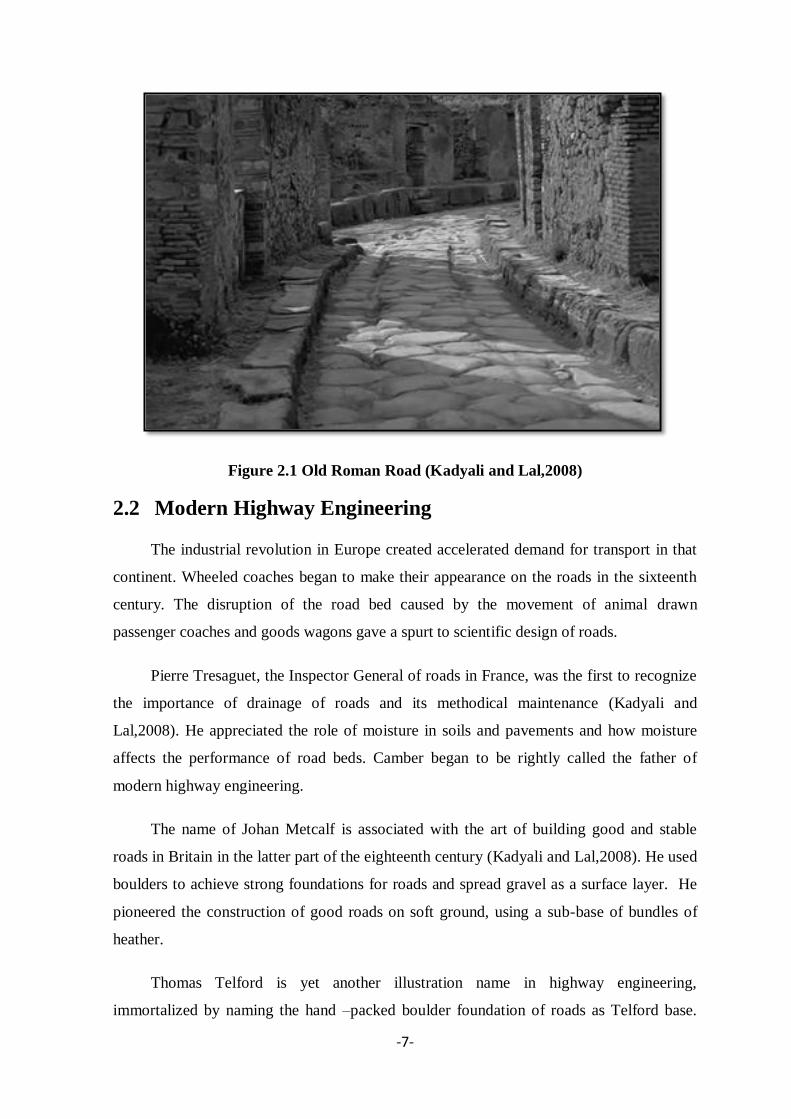
-7-
Figure 2.1 Old Roman Road (Kadyali and Lal,2008)
2.2 Modern Highway Engineering
The industrial revolution in Europe created accelerated demand for transport in that
continent. Wheeled coaches began to make their appearance on the roads in the sixteenth
century. The disruption of the road bed caused by the movement of animal drawn
passenger coaches and goods wagons gave a spurt to scientific design of roads.
Pierre Tresaguet, the Inspector General of roads in France, was the first to recognize
the importance of drainage of roads and its methodical maintenance (Kadyali and
Lal,2008). He appreciated the role of moisture in soils and pavements and how moisture
affects the performance of road beds. Camber began to be rightly called the father of
modern highway engineering.
The name of Johan Metcalf is associated with the art of building good and stable
roads in Britain in the latter part of the eighteenth century (Kadyali and Lal,2008). He used
boulders to achieve strong foundations for roads and spread gravel as a surface layer. He
pioneered the construction of good roads on soft ground, using a sub-base of bundles of
heather.
Thomas Telford is yet another illustration name in highway engineering,
immortalized by naming the hand –packed boulder foundation of roads as Telford base.

-8-
The construction technique held the sway for nearly 150 years since Telford introduced it
in the early part of the nineteenth century (Kadyali and Lal,2008).
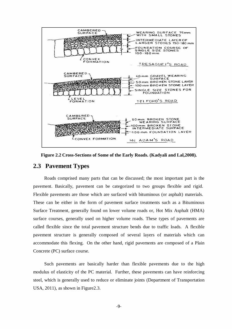
A run of names of eminent highway engineers is incomplete without John Mc
Adam’s. He was a Scottish road builder who was influenced road construction so
profoundly that the term “macadam” is frequently used in pavement specification even to
this day. His two important principles of good road construction were:
It is the native soil that supports the traffic load ultimately, and when the soil is maintained
in dry state it can carry heavy loads without settlement.
Stones which are broken to small angular pieces and compacted can interlock with each
other and form a hard surface.
Thus, Mc Adam’s specifications were at variance with Telford’s in that small pieces
of stones with angular faces were favored than larger hand-packed boulders. He was
reported to give a practical hint to engineers in selecting the size of stones; the size is good
if the stone cane be put into the mouth. How valid his advice is even to this day! Apart
from the innovative specifications he introduced, Mc Adam is also remembered for his
foresight in urging the creation of a central highway authority to advice and monitors all
matters relating to roads in Britain. (Figure 2.2) gives the cross-sections of some of the
early roads.
A significant development which revolutionized road construction during the nineteenth
century was the steam road roller introduced by Eveling and Barford.
The development Portland cement in the first few decades of the nineteenth century by
Aspdin and Johnson facilitated modern bridge construction and use of concrete as a
pavement material (Kadyali and Lal,2008).
Tars and asphalts began to be used in road construction in the 1830s, though it was
pneumatic tyre vehicle which gave real push to the extensive use of bituminous
specifications.
-9-
Figure 2.2 Cross-Sections of Some of the Early Roads. (Kadyali and Lal,2008).
2.3 Pavement Types
Roads comprised many parts that can be discussed; the most important part is the
pavement. Basically, pavement can be categorized to two groups flexible and rigid.
Flexible pavements are those which are surfaced with bituminous (or asphalt) materials.
These can be either in the form of pavement surface treatments such as a Bituminous
Surface Treatment, generally found on lower volume roads or, Hot Mix Asphalt (HMA)
surface courses, generally used on higher volume roads. These types of pavements are
called flexible since the total pavement structure bends due to traffic loads. A flexible
pavement structure is generally composed of several layers of materials which can
accommodate this flexing. On the other hand, rigid pavements are composed of a Plain
Concrete (PC) surface course.
Such pavements are basically harder than flexible pavements due to the high
modulus of elasticity of the PC material. Further, these pavements can have reinforcing
steel, which is generally used to reduce or eliminate joints (Department of Transportation
USA, 2011), as shown in Figure2.3.

-10-
Figure2.3 Rigid and Flexible Pavement Load Distribution(W. and Lenz, 2011)
2.4 Hot Mix Asphalt Pavement
Asphalt pavements are composed of skeleton of coarse and fine aggregates and a
filler of aggregate dust, asphalt cement as a binder and air voids as shown in Figure 2.4.
Three groups of aggregates are usually used in asphalt concrete mix design. These are
coarse aggregate, fine aggregate and mineral filler.
Figure2.4 Diagram Aggregate Frame Work with Asphalt Binder and Air
Voids(Kadyali and Lal,2008).

-11-
A successful flexible pavement must have several desirable properties. These are
stability, durability, safety (skid-resistance) and economy. Because of the binding property
of asphalt cement, it is the most important constituent in asphalt concrete mix. Quality
control of asphalt cement is always required and essential for successful mix performance.
Some of these control quality tests are performance grading (PG), penetration, softening
point, ductility, flash point, thin- film oven test, solubility, viscosity, etc. Asphalt content is
a very important factor in the mix design and has a bearing on all the characteristics of a
successful pavement. Various mix design procedures are used for finding out the
“optimum” asphalt content.
2.5 Hot Mix Asphalt Design Methods
All of (HMA) design methods must govern the following considerations:
1. The binder content should be sufficient to impart the maximum stability. For a
given mix grading, there is an optimum binder content that produce maximum
stability.
2. The binder content should be to impart workability to the mix to facilitate its
placement.
3. The voids in the aggregates should partly fill by bitumen and partly left unfilled.
The unfilled voids will act a reservoir of space for the expansion of the asphalt
during hot days and for a slight amount of additional compaction under traffic
loading. Overfilling of the voids with binder may result in bleeding of asphalt and
should be avoided.
4. The durability of the pavement is governed by the binder content. The higher the
binder content, the more durable is the mix.
Some of the above considerations are conflicting in requirements. Therefore, the
selection of the binder content has to be a judicious compromise.
There are four popular methods of (HMA) design(Kadyali and Lal,2008):
Marshall method
Hubbard-Field method
-12-
Hveem method
Smith traxial method
Each of the above methods is associated with a set of design criteria for the properties of
the mix. The Marshall method is the most popular in Egypt and is described below.
2.6 Marshall Method
The Marshall method of mix design has been widely used with satisfactory results. It
was developed originally by Bruce Marshall of the Mississippi State Highway Department.
The U.S. corps of engineers had been later developed and adopted it.
2.6.1 Specimen Preparation
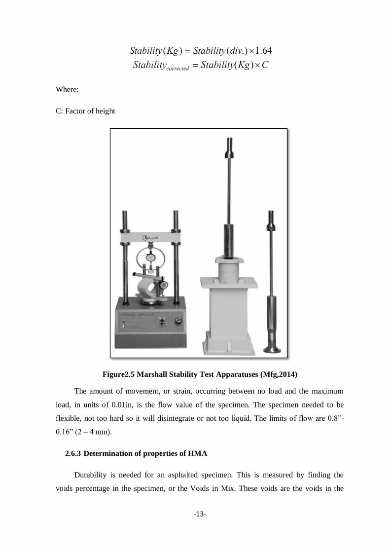
The test is relatively a simple one and uses simple apparatus. In the test a sample
specimen 4in in diameter and 2½in high is prepared by compacting in a mould on both
faces with a compacting hammer shown in Figure 2.5. That weighs 10lb and has a free fall
of 18in depending upon the design traffic condition
For heavy traffic use 75 strokes at both sides of sample
For medium traffic use 50 strokes at both sides of sample
For light traffic use 35 strokes at both sides of sample
After overnight curing, the density and voids are determined and the specimen is
heated to 140ºF (60ºC) for the Marshall Stability and flow tests. Our study will be made on
heavy loading criteria.
The specimen is then placed in a cylindrically shaped split breaking head and is
loaded at a rate of 2in/min. The maximum load registered during the test in Newton or
pounds is designated as the Marshall stability of the specimen. The stability we want to get
is bigger than or equals 750Kg.
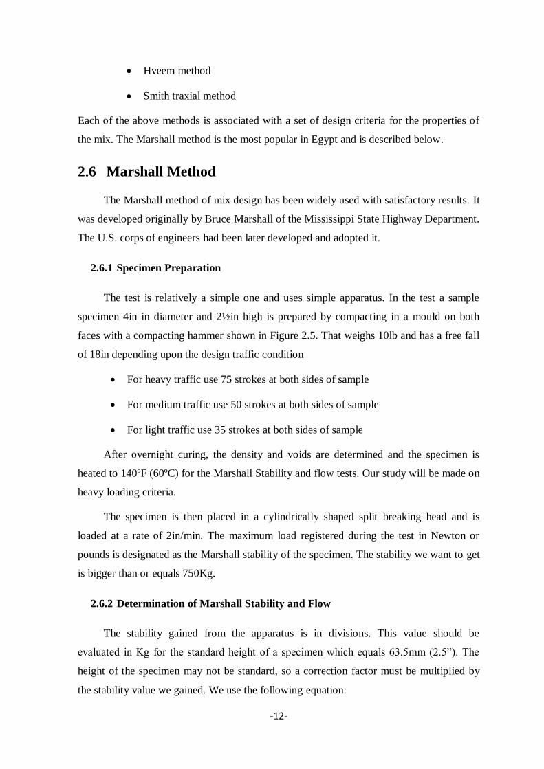
2.6.2 Determination of Marshall Stability and Flow
The stability gained from the apparatus is in divisions. This value should be
evaluated in Kg for the standard height of a specimen which equals 63.5mm (2.5”). The
height of the specimen may not be standard, so a correction factor must be multiplied by
the stability value we gained. We use the following equation:
-13-
Where:
C: Factor of height
Figure2.5 Marshall Stability Test Apparatuses (Mfg,2014)
The amount of movement, or strain, occurring between no load and the maximum
load, in units of 0.01in, is the flow value of the specimen. The specimen needed to be
flexible, not too hard so it will disintegrate or not too liquid. The limits of flow are 0.8”-
0.16” (2 – 4 mm).
2.6.3 Determination of properties of HMA
Durability is needed for an asphalted specimen. This is measured by finding the
voids percentage in the specimen, or the Voids in Mix. These voids are the voids in the

-14-
mix after compaction having the range of 3-5% with 4% for medium load. Less than 3%
voids ratio means no enough space for bitumen to fill the sample and carry the load. While
more than 5% ratio means a very high porous specimen, thus, ease for water and air to
flow inside and therefore lead to segregation.
It has been noticed that after long term use of the road, the voids ratio will decrease
because of compression under load. So a correction for the limit is used, that is (4-6) % so
that the voids ratio will go back to its original limit after compaction. There are five
measurements we can use them:
The theoretical specific gravity Gt. the bulk specific gravity of the mix Gm. percent
air voids Vv. percent volume of bitumen Vb. percent void in mixed aggregate VMA and
percent voids filled with bitumen VFB.
These calculations are discussed next. To understand these calculations a phase
diagram is given in (Figure 2.6).
Figure2.6 Marshall Mould (Mathew and Krishna Rao,2006)
2.6.4 Theoretical specific gravity of the mix Gt
Theoretical specific gravity Gt is the specific gravity without considering air voids,
and is given by:

-15-
(1)
Where,
W1 is the weight of coarse aggregate in the total mix,
W2 is the weight of fine aggregate in the total mix,
W3 is the weight of filler in the total mix,
Wb is the weight of bitumen in the total mix,
G1 is the apparent specific gravity of coarse aggregate,
G2 is the apparent specific gravity of fine aggregate,
G3 is the apparent specific gravity of filler
Gb is the apparent specific gravity of bitumen,
2.6.5 Bulk specific gravity of mix Gm
The bulk specific gravity or the actual specific gravity of the mix Gm is the specific
gravity considering air voids and is found out by:
(2)
Where,
Wm is the weight of mix in air,
Ww is the weight of mix in water,
2.6.6 Air voids percent Vv
Air voids Vv is the percent of air voids by volume in the specimen and is given by:

-16-
(3)
Where
Gt is the theoretical specific gravity of the mix, given by equation (1).
Gm is the bulk or actual specific gravity of the mix given by equation (2).
2.6.7 Percent volume of bitumen Vb
The volume of bitumen Vb is the percent of volume of bitumen to the total volume
and given by:
(4)
Where,
W1 is the weight of coarse aggregate in the total mix,
W2 is the weight of fine aggregate in the total mix,
W3 is the weight of filler in the total mix,
Wb is the weight of bitumen in the total mix,
Gb is the apparent specific gravity of bitumen,
Gm is the bulk specific gravity of mix given by equation (2).
2.6.8 Voids in mineral aggregate VMA
Voids in mineral aggregate VMA is the volume of voids in the aggregates, and is the
sum of air voids and volume of bitumen, and is calculated from
VMA = Vv + Vb (5)
Where,

-17-
Vv is the percent air voids in the mix, given by equation (3).
Vb is percent bitumen content in the mix, given by equation (4).
2.6.9 Voids filled with bitumen VFB
Voids filled with bitumen VFB is the voids in the mineral aggregate frame work
filled with the bitumen, and is calculated as:
(6)
Where,
Vb is percent bitumen content in the mix, given by equation (4).
VMA is the percent voids in the mineral aggregate, given by equation (5).
An additional useful term is Stiffness.
2.7 Controlling Quality During Construction
2.7.1 Frequency of tests for quality control
Quality control during construction is necessary to ensure that the pavement is
constructed so as to meet the various requirements of specifications and design documents.
Such a quality control involves a variety of tests to be conducted during construction with
regular frequency and obtaining all the relevant construction data for statistically
processing the test results. The different types of tests to be conducted and their repetitions
for earthwork , granular sub bases and base courses, pavement layers involving
bituminous and cement concrete construction work are given in table 2.1 below.

-18-
Table 2.1 Frequency of tests for quality control(Kadyali and Lal,2008).
NO. Item of work Test Frequency Rate Notes
1 Earthwork
Soil particle size,
Atterberg Limits 1-2 tests 8000 m
3
C.B.R on a set of 3
specimens 1 test 3000 m
3
Natural moisture
content 1 test 250 m
3
Moisture content
before compaction 2-3 tests 250 m
3
Dry density of
compacted area 1 test 1000 m
3
Embankments to be
increased to one
test per 500-1000
m3 for sub grade
layers.
2 Gravel sub-base
Gradation, plasticity 1 test 200 m3
Moisture content 1 test 250 m3
Density 1 test 500 m3
3 Lime – soil
Purity of lime 1 test 5Ton
Lime content,
moisture content 1 test
250 m2

-19-
3 Lime – soil
Density 1 test 500 m2
4
Water-bound
macadam
Los Angeles
Abrasion or
Aggregate Impact
Value, Flakiness
Index
1 test 200 m
3
Grading of materials 1 test 100 m
3
Plasticity of binder 1 test 25 m3
5
Bituminous
Macadam
Los Angeles
Abrasion Value or
Aggregate
1 test 50-100
m3
Mix grading, binder
content, aggregate
gradation
2 tests day
6
Surface
dressing and
premix carpet
Los Angeles
Abrasion
Value or Aggregate
Impact
Value, Stripping
Value, Flakiness
Index
Water absorption
1 test 50 m3
Grading of aggregate 1 test 25 m
3
Rate of spread of
binder and aggregate
for surface dressing
1 test 500 m3
Binder content for
premix carpet 2 test day

-20-
7
Hot mix
Asphalt
Los Angeles
Abrasion Value or
Aggregate, Impact
Value, Stripping
Value, Water
absorption, Flakiness
Index
1 test
50-100
m3
Sieve analysis for
filler 1 test
100 ton
of mix
Mix grading, binder
content
1 test 100 ton min. 3 tests per day
Stability and flow
Thickness and
density
3 Marshall
Specimens
1000
ton
8
Cement
concrete
pavement
Gradation of
aggregate
Cement, physical
and chemical
Concrete strength
1 test
Los Angeles
Abrasion Value or
Aggregate
1 test
Impact Value,
Soundness
1 test
-21-
8
Cement
concrete
pavement
Workability
3
cube/beam
samples for
each 7 days
and 28 days
30 m3
Concrete strength on
hardened concrete 2 cores 30 m
3
2.7.2 Scope at Hot mix asphalt Q.C frequency
According to the previous table at Hot Mix Asphalt section it shown that for
controlling quality during construction Mix grading (sieve analysis) and binder content
(bitumen extraction) were conducted minimum 3 tests per day or one test per 100T of mix,
Stability and flow (Marshall test ) (AASHTO-T245,2006) conducted also 3 specimens per
100T of mix, so those tests are daily tests in site which can be correlated together .
2.8 Sieve Analysis for Fine and Coarse Aggregates
This test method determines the particle size distribution of fine and coarse
aggregates by sieving. The No. 4 sieve is designated as the division between the fine and
coarse aggregate Figure 2.7.
2.8.1 Procedure:
Dry the sample according to T 255 at a temperature of 230 ± 9°F (110 ± 5°C). Select
sieves to furnish the information required by the specifications covering the material to be
tested. Use of additional sieves may be desirable to prevent the required sieves from
becoming overloaded.
The quantity retained on any sieve, with openings smaller than the No. 4 sieve, at the
completion of the sieving operation shall not exceed 4 g per sq.in. of sieving surface area.
If this occurs it is considered overloading of the sieve. The overload amount for an 8"
diameter sieve is 200 g.

-22-
Figure2.7 The Sieve Shaker with a Stack of Sieves.(instruments,2014)
Table 2.2 Shows different size sieves of the maximum allowable quantities of
material retained on a sieve (AASHTO-T-27,2006).
Table 2.2 Different Size Sieves of the Maximum Allowable Quantities of
Material Retained on a Sieve(AASHTO-T-27,2006).
-23-
2.8.2 Calculation:
Add the non-cumulative weight retained on the largest sieve to the weight retained
on the next smallest sieve and record in the cumulative column.
Calculate the percent retained on each sieve by dividing each weight by the original
total dry weight and multiply by 100. This is the percent retained. Subtract each of these
values from 100 to obtain the percent passing each sieve. Continue this process for each
sieve. The equations are as follows:
Percent retained on sieve = (Cumulative weight/Total weight) x 100
Percent passing = 100 - Percent retained on sieve
This calculation is completed for both the course and fine aggregate.
If an accurate determination of the amount of material passing the No. 200 was
accomplished by performing T 11, subtract the weight after wash from the original weight
and record as wash loss.
Sum the cumulative weight retained on the No. 200, the weight of the Minus No. 200
material, and the wash loss, and record as the weight check.
To calculate the percent passing of the total sample for the fine portion of the
aggregate, multiply the percent passing the sieve No. 4 multiply by the percent passing on
each individual. Sieve in the fine aggregate portion and divide by 100. The equation is as
follows:
Percent total sample = [(Percent passing No.4) x (Percent passing smaller sieve)]/100
Final calculations of percentages passing are reported to the nearest whole number
with the exception of the No. 200 which is reported to same significant digit as specified
by the specification for the class of aggregate.
For both the Plus No. 4 and Minus No. 4, compare the original weight to the weight
check. Subtract the smaller value from the larger value, divide the result by the original
weight, and multiply by 100, to obtain the percent difference. For acceptance purposes, the
two must not differ by more than 0.3%.

-24-
2.9 Bitumen Extraction Test
The method described is a procedure used to determine the bitumen content of
bitumen aggregate mixtures according to(ASTM-D2127).
2.9.1 Apparatuses and materials:
Centrifuge extractor with a bowl. The extractor must be capable of rotating the bowl
at controlled variable speeds up to 3600 rpm as shown in Figure 2.8.
Paper or felt filter rings to be placed on the rim of the bowl and beneath the bowl lid.
Scale capable of weighing to 2500 g at 0.1 g accuracy.
Heating equipment such as electric stove.
500 ml cup or beaker.
Hand Tools - spatula, small brush, scoop, large pan for collection of a representative
bitumen mix sample, pan for test sample.
Container for collection of bitumen laden solvent thrown from the bowl during
extraction.
Solvents - suggested materials are benzene or Carbon Tetra chloride.
Figure2.8 Bitumen Extractor (Centrifuge Extractor)(Mfg,2014)
-25-
2.9.2 Procedure
A representative sample about 400gm is exactly weighed and placed in the bowl of
the extraction apparatus and covered with commercial grade of benzene. Sufficient time
(not more than 1 hour) is allowed for the solvent to disintegrate the sample before running
the centrifuge.
The filter ring of the extractor is dried, weighed and then fitted around the edge of
the bowl. The cover of the bowl is clamped tightly. A beaker is placed below to collect
the extract.
The machine is revolved slowly and then gradually, the speed is increased to a
maximum of 3600 r.p.m. The speed is maintained till the solvent ceases to flow from the
drain. The machine is allowed to stop and 200 ml. of the benzene is added and the above
procedure is repeated.
A number of 200 ml. solvent additions (not less than three) are used till the extract is
clear and not darker than a light straw color.
The filter ring from the bowl is removed, dried in air and then in oven to constant
weight at 115o C and weighed. The fine materials that might have passed through the
filter paper are collected back from the extract preferably by centrifuging. The material is
washed and dried to constant weight as before.
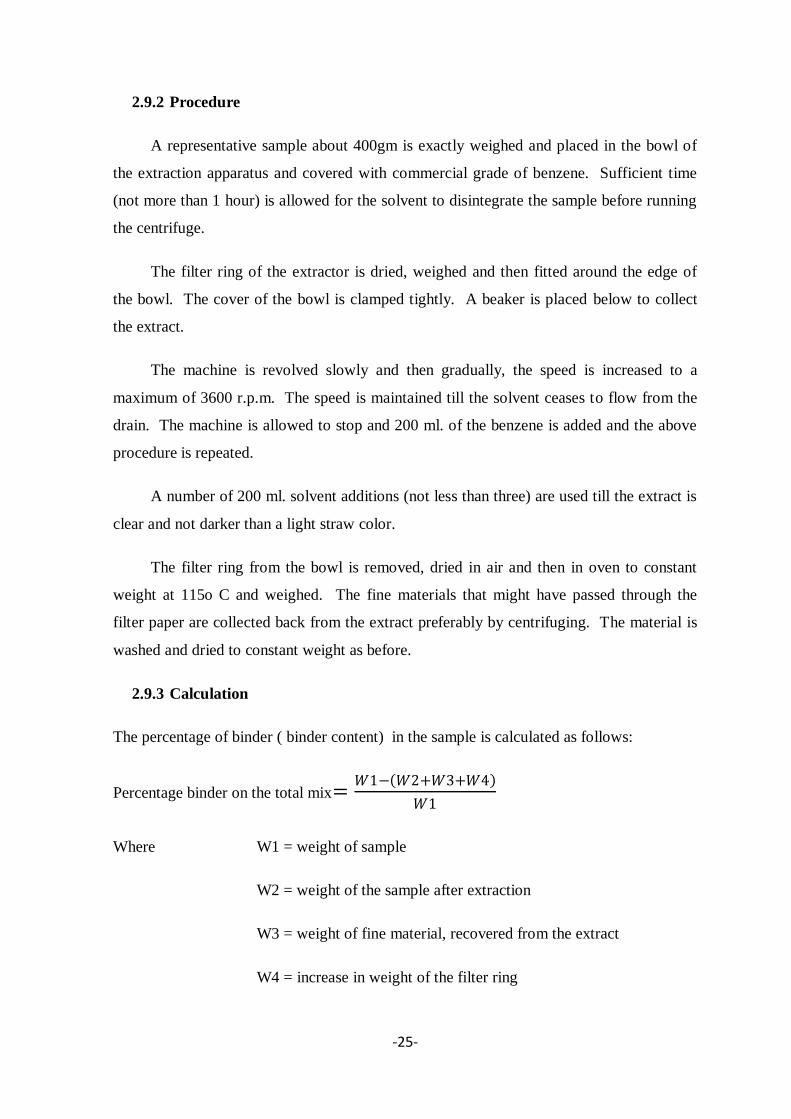
2.9.3 Calculation
The percentage of binder ( binder content) in the sample is calculated as follows:
Percentage binder on the total mix=𝑊1− 𝑊2+𝑊3+𝑊4
𝑊1
Where W1 = weight of sample
W2 = weight of the sample after extraction
W3 = weight of fine material, recovered from the extract
W4 = increase in weight of the filter ring

-26-
2.9.4 Application of testes
The bitumen content of bitumen-aggregate mixtures as determined by the described
test method is used for
Product acceptance.
Quality assurance.
Quality control
Research activities.
2.10 Modern Prediction Techniques
Different fields of engineering aims to estimate final results from previous recorded
data. There are many kinds of prediction techniques such as:
Artificial neural network.
Linear and multiple regressions.
Hypothetical frame work.
Generally, the first artificial neural network (ANN) paper in civil engineering area
was published in 1989 (Adeli ,et al.,2001). (Adeli ,et al.,2001) identified the neural
networks as “a function of the biologic neural structures of the central nervous system.”
Previously, researchers in the area of civil engineering used ANNs as a reliable tool
for simulation and regression analysis. According to (Flood,2006), the artificial neural
networks have been identified as the more flexible and precise method for all academic
researches and some practical achievements. Flood pointed out the artificial neural network
as reasonable and interesting research implemented in computer based civil engineering.
However, the researchers are challenged to come up with a complete and convincing
prediction model in the future (Flood,2006).
According to(Adeli and Wu,1998), a regularization neural network model was
created to forecast the estimated construction cost of projects.
Another publication implements the back propagation network (BPN) model based
on genetic algorithms to estimate construction projects cost(Kim ,et al.,2004).

-27-
(Kim ,et al.,2004)attempted to construct prediction models by two distinct methods;
back propagation network (BPN) genetic algorithm and trial and error comparing the
result. This attempt concluded that a BPN model incorporating a genetic algorithm
determines reliable and accurate construction estimation compared to the trial and error
method.
The artificial neural network methods and models represent broad usage in terms of
simulation and statistical analysis in science and arts. A research was accomplished in
terms of framework to develop, train, and test neural network to predict concrete act ivities
estimation (Ezeldin and Sharara,2006). This attempt identified the influential factors in
concrete activities and developed a prediction model based on the identified parameters.
The data used for accomplishment of this research was collected in Egypt. As a result
of this research, the identification of influential factors demonstrates reasonable
improvement to predict future values.
On the other hand, distinct to ANNs, models were developed based on linear
regression analysis to predict the construction projects costs. An attempt of regression
modeling used 286 records of data in the United Kingdom to develop forecasting models
(Lowe ,et al.,2006). The models were created based on; cost/m2, log of cost and log of
cost/m2. In this analysis backward and forward stepwise analysis was preferred. In
addition, regression analysis and bootstrap methods were also implemented for the
conceptual estimation of costs. The author concluded the advantage of this method as both
techniques used for the same inputs with fewer assumptions(Lowe ,et al.,2006).
Also, (Sonmez 2004), emphasized advantages and disadvantages of conceptual cost
estimation methods. In this investigation intangible cost models were developed based on
regression analysis and neural networks to compare the method reliability. The researcher
of this paper eager was to use simultaneously the regression analysis and neural network a
leading step to the future of more realistic expectation and better strategies. A reliable
advantage of simultaneously using both methods demonstrates the convenience of
accuracy.
The third technique, a hypothetical frame work was performed to identify the
critical issues of effective cost judgment during each stage of project (Liu ,et al.,2007).
This work has classified the critical issues and relationship between the dependent and

-28-
independent factors. (Liu ,et al.,2007), concluded the approach to be helpful for future
construction companies to control the critical factors for an effective predicted estimation.
In another attempt,(Skitmore and Ng,2003), developed several models based on 93
construction projects to predict the actual construction time. This analysis identified the
influential parameters in project duration prediction as the method of contractors‟ selection
of imprecise contract phase and sum, and cost based on the risk and doubts of different
segments (Skitmore and Ng,2003). In another hand, an investigation was performed to
incorporate the parametric and probabilistic cost assessment procedures as well (Sonmez
2004).
2.11 Introduction to Neural Networks
Based on many techniques and methods used to maintain the previous data and
develop future forecasting models, mathematical regression analysis have been widely
used(Aasadullah. Attal,2010). Based on the statistical analysis “Artificial Neural Networks
(ANN) recently been broadly used to model some of the human activities in many areas of
science and engineering” (Rafiq ,et al.,2001). Nevertheless, the previous historical data
and expert represents crucial implements for future improvement.
According to (Moselhi ,et al.,1991), currently there have been several artificial
intelligences such as expert systems, robotics , and neural networks used for statistical
analysis. In this study, expert system was identified as an attempt to model the problem
solution based on the capability of human brain. On the other hand, neural network efforts
to model the brain learning, thinking, storage, and retrieval of information, as well as
associative recognition” (Moselhi ,et al.,1991). Therefore, this research attempts to identify
the input-output relationship and improve future highway construction data forecasts based
on nonlinear ANNs and linear regression analysis.
A research pointed out that: “Artificial Neural Networks (ANNs) are mathematical
models, which are biologically inspired to imitate the primitive cognitive functionality of
the human brain” (Young II ,et al.,2008). The artificial intelligence model names machine
learning represents data-driven is capable of showing complex input and output non-linear
relationships (Young II ,et al.,2008).
Since the ANNs have been identified as universal approximator (Reed and Marks,1998),
therefore a structured approach was performed to develop the non-linearity of modeling.
-29-
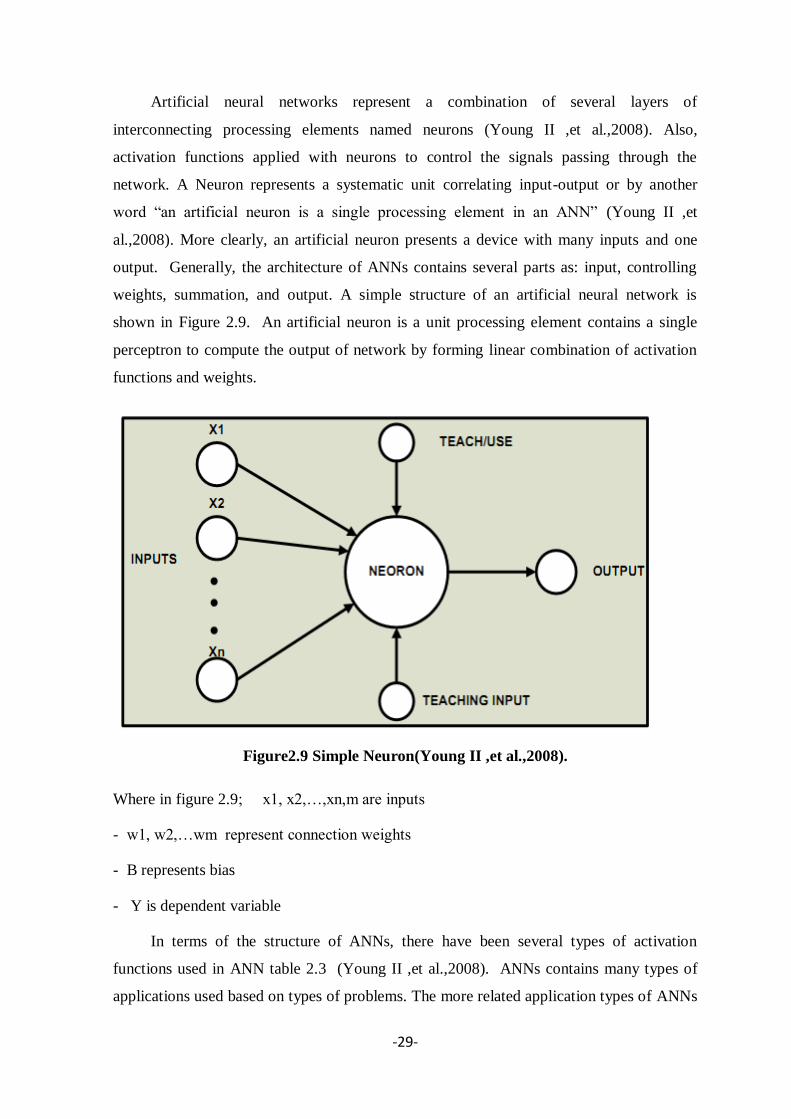
Artificial neural networks represent a combination of several layers of
interconnecting processing elements named neurons (Young II ,et al.,2008). Also,
activation functions applied with neurons to control the signals passing through the
network. A Neuron represents a systematic unit correlating input-output or by another
word “an artificial neuron is a single processing element in an ANN” (Young II ,et
al.,2008). More clearly, an artificial neuron presents a device with many inputs and one
output. Generally, the architecture of ANNs contains several parts as: input, controlling
weights, summation, and output. A simple structure of an artificial neural network is
shown in Figure 2.9. An artificial neuron is a unit processing element contains a single
perceptron to compute the output of network by forming linear combination of activation
functions and weights.
Figure2.9 Simple Neuron(Young II ,et al.,2008).
Where in figure 2.9; x1, x2,…,xn,m are inputs
- w1, w2,…wm represent connection weights
- B represents bias
- Y is dependent variable
In terms of the structure of ANNs, there have been several types of activation
functions used in ANN table 2.3 (Young II ,et al.,2008). ANNs contains many types of
applications used based on types of problems. The more related application types of ANNs

-30-
in engineering area represents: adaptive controller, interpretation system, machining
feature recognition system, image classification system, and a pump design system (Garrett
et al., 1993). In addition to that, other applications used in engineering, formed in the
following list:
1. Stochastic contains the approximation ability(Belli ,et al.,1999).
2. Functional networks for in real-time flood forecasting- a novel application (Bruen
and Yang,2005).
3. Genetic algorithms (GA) for the permeability estimation of the reservoir, fuzzy
neural networks for the design of industrial roofs (Rajasekaran ,et al.,1996).
4. Back-propagation learning algorithm used in a research for prestressed concrete
pile (Tam ,et al.,2004).
5. Discrete - event simulation used for modeling of construction processes(Flood and
Worley,1995).
6. Fuzzy neural inference model used for conceptual construction cost estimation
(Cheng ,et al.,2009).
Also, a research was provided to develop a neural network based on decision making
system –neuro mode for an industrial plant (Murtaza and Fisher,1994). In this research,
several major attributes categorized to provide the decision based on Neural Networks
(NN) represents; plant location, environmental and organizational, labor-related, plant
characteristics and project risks (Murtaza and Fisher,1994).
In addition, an experimental assessment of neural network was accomplished for
nonlinear time-series forecasting(Zhang ,et al.,2001). This research concluded the neural
network is a reliable tool for forecasting nonlinear time series. The impact of input, hidden
layers, and output nodes were practically examined (Zhang ,et al.,2001).
The ability of ANNs to adapt different types of problems based on activation
functions represents a critical flexibility. These functions experimentally change based on
the placed independent variables in model and expected outputs. The mathematical
activation functions used in ANNs to interpret the data between layers and input-output
placed in table 2.3.

-31-
The NN approach with simulated data showed a promising result. However,
according to(Chao and Skibniewski,1995) , several assumptions have been used in the
simulation modeling which might cause low precision.
Accordingly, a procedure was developed based on the neural networks model to
escalate the highway construction costs over time considering highway construction cost
index (Wilmot and Mei,2005). The influential terms in this cost index model represent the
costs of: construction material, labor, equipment, and the time of notice to proceed.
Based on the mentioned flexibility of ANNs, a neural networks data-base was
accomplished to estimate the construction operation productivity (Chao and
Skibniewski,1994). This attempt examined an excavation process by excavator and
concluded that neural networks are an efficient tool for construction productivities
estimation. Also, a neural network based approach was developed to forecast the
acceptability of new construction technology(Chao and Skibniewski,1995).
In this study a neural network model and linear regression models were simultaneously
developed to evaluate labor productivity in construction projects but ANNs came up with
reasonable higher accuracy compared to regression analysis(Sonmez and Rowings,1998).
This model was examined on concrete pouring, formwork, and concrete finishing tasks.
The general mathematical equation used for calculation of network is presented in the
following equation:
Where, in this equation
Wki is the controller weight of input i to the hidden layer k, So is the hidden layer-
output activation function, xi is the input i,
Wko is the weight of hidden layer to output.
Wk, Wo is the respectively weight of input k, hidden layer to output on the same
example.

-32-
Table 2.3 Common Activation Functions in ANNs (Adapted from Young II et al, 2008)
Activation Functions Definitions Range
Linear x (-∞,+∞)
Sigmoid
1
(1 − 𝑒−𝑥)
(0 , 1)
Hyperbolic
𝑒𝑥 − 𝑒−𝑥
(𝑒𝑥 + 𝑒−𝑥)
(-1 , 1)
Exponential 𝑒−𝑥 (0 , ∞)
Soft max
𝑒−𝑥
𝑥𝑖𝑖
(0 , 1)
Unit Sum
𝑥
𝑥𝑖𝑖
(0 , 1)
Square Root 𝑥 (0 , ∞)
Sine Sin(x) (0 , 1)
Ramp 1 , 𝑥 ≤ −1
𝑥,−1 < 𝑥 < 11 ,𝑥 ≥ 1
(-1 , 1)
Step 0 ,𝑥 < 01 ,𝑥 ≥ 0
(0 , 1)
Where in this equation: Yi represents the observed value and Ŷi is the mean value.
The sub i represents an integer from 1 to n.
The mathematical equation used for mean square error is formulated in the
following equation:

-33-
Where Yi is the observed value and Ŷi is predicted value, and i is an integer varying
from 1 to n. In this equation instead of n (Y-Ȳ)2 is used in some analysis to determine the
final error.
Based on the mentioned information, a method was derived to combine some of the
recent useful methods and traditional symbolic systems to develop the reliability of
prediction and classification models(Fletcher and Hinde,1995). This research pointed out
the neural networks as a reliable tool for highway Marshall Test prediction. The
architecture of an ANNs model approximate assumed for this prediction model is shown in
Figure 2.10.
Figure2.10 Simple Architecture of Prediction Model Based on ANNs
There are several types of artificial neural networks and regression analysis software
to classify or predict the future values based on the past data. The models developed in this
research based on the knowledge and calculation and procedure respectively based on the
Neuro Solutions for Excel and Automated Neural system of STATISTICA for ANNs and
Minitab and multiple regression of STATISTICA for stepwise regression analysis.
However, the results of models that placed in this research entirely calculated by
Automated Networks (ANs). The reason for the choosing of ANs for the calculation of

-34-
these models represents the ability of the system that calculating the model faster and most
importantly automatically choosing.
Where, Ski, abs is the average sensitive absolute value of partial derivative of output k
with respect to input i, and p is the number of samples.
2.12 Historical Background of Neural Network Applications in
Pavement Engineering
Very detailed information about the applications of traffic engineering can be found
in the relevant literature (Tapkın,2004). At this point, it is important to state out, one by
one, the relevant important neural network applications in the pavement engineering area.
In a study by (Ritchie ,et al.,1991), a system that integrates three artificial intelligence
technologies: computer version, neural networks and knowledge-based system in addition
to conventional algorithmic and modeling techniques were presented. (Ritchie ,et al.,1991)
used neural network models in image processing and pavement crack detection.(Gagarin
,et al.,1994) discuss the use of a radial-Gaussian-based neural network for determining
truck attributes such as axle loads, axle spacing and velocity from strain-response readings
taken from the bridges over which the truck is traveling.
(Eldin,1995) describe the use of a back propagation (BP) algorithm for condition rating of
roadway pavements. They report very low average error comparing with a human expert
determination , (Cal,1995) uses the back propagation algorithm for soil classification based
on three primary factors: plastic index, liquid limit, water capacity, and clay content.
(Razaqpur ,et al.,1996) present a combined dynamic programming and Hopfield neural
network bridge-management model for effi-allocation of a limited budget to bridge
projects over a given period of time.
The time dimension is modeled by dynamic programming, and the bridge network is
simulated by the neural network. (Roberts and Attoh-Okine,1998) use a combination of
supervised and self-organizing neural networks to predict the performance of pavements as
defined by the International Roughness Index.(Tutumluer and Seyhan,1998) investigated

-35-
neural network modeling of anisotropic aggregate behavior from repeated load triaxial
tests.
The BP algorithm is used by (Owusu-Ababia,1998) for predicting flexible pavement
cracking and by (Alsugair and Al-Qudrah,1998) to develop a pavement-management
decision support system for selecting an appropriate maintenance and repair action for a
damaged pavement.
(Kim and Kim,1998) used artificial neural networks for prediction of layer module
from falling weight deflectometer (FWD) and surface wave measurements.
(Shekharan,1998) studied the effect of noisy data on pavement performance
prediction by an artificial neural network with genetic algorithm.
(Attoh-Okine,2001) uses the self-organizing map or competitive unsupervised
learning model for grouping of pavement condition variables (such as the thickness and
age of pavement, average annual daily traffic, alligator cracking, wide cracking, potholing,
and rut depth) to develop a model for evaluation of pavement conditions.
(Lee and Lee,2004) present an integrated neural network-based crack imaging
system to classify crack types of digital pavement images which includes three types of
neural networks: image-based neural network, histogram-based neural network and
proximity-based neural network.
In an article by (Mei ,et al.,2004), it is presented a computer-based methodology with
which one can estimate the actual depths of shallow, surface-initiated fatigue cracks in
asphalt pavements based on rapid measurement of their surface characteristics.
(Ceylan ,et al.,2005) has investigated the use of artificial neural networks as
pavement structural analysis tools for the rapid and accurate prediction of critical responses
and deflection profiles of full-depth flexible pavements subjected to typical highway
loadings.
(Bosurgi and Trifiro,2005) has described a procedure that has been defined to make
use of the available economic resources in the best way possible for resurfacing
interventions on flexible pavements by using artificial neural networks and genetic
algorithms.

Chapter Three
DATA COLLECTION TECHNIQUES
AND CLASSIFICATION

-37-
Chapter 3
DATA COLLECTION TECHNIQUES AND
CLASSIFICATION
3.1 Introduction
This chapter outlines the data sources and parameters used in the analytical work of
this research. Collecting data is the most difficult and critical part for its importunacy in the
research which all the work is depending on it. On this research the data is extracted from
real laboratory and site experimental.
3.2 Description of Data
The data in this thesis was collected and extracted from two main processes:
Job mix design tests process
Quality control tests process
From (HMA) of highway project (BaniSwef-El-Minya - Assyutfree way Project)
constructed in Upper Egypt. The satellite image below (Figure3.1) shows the location of
the highway which parallel to the old road at the east bank of Nile River.
This project was about 320 km long , about 121 km from Baniswef city to El-Minya
city and about 121 km from El-Minya city to Assyut city .
The cross section (Figure3.2) was three lanes for each way with 2.5 m outer paved
shoulders, 0.75m inner paved shoulders, 20 m median with total width 52 m, the project
has a huge quantity of earth moving working, it was about 37 million m3 of fill and
11million m3 of cut, the paving work had about 19 million m
2 of (HMA).
3.2.1 Data collection
Data were collected from two main sources:
Different trials of job mix for (HMA) design which was done at laboratory.
Quality control actual tests which were done mainly at site.

-38-
Figure 3.1 The Layout of the Highway

-39-
Figure 3.2 The Typical Cross Section of the Highway
3.2.2 Job mix of asphalt
Marshall Specimens were fabricated in the laboratory utilizing75 blows on each face
representing heavy traffic conditions according to (AASHTO-T245,2006). The standard
60/70 penetration bitumen was modified in the laboratory.
Marshall Stability and flow tests were done on these asphalt samples. These tests were
considered to be adequate to clarify the positive effect of different mixes on asphalt
concrete. In laboratory test program, continuous aggregate gradation has been used to fit
the gradation limits for wearing course set by Highway Technical Specifications of
General Association of Egypt Highways and Bridges (Highway Technical Specifications,
1998). The aggregate was calcareous type crushed stone obtained from a local quarry and
60/70 penetration bitumen obtained from a local refinery (El-Nasr Company) in Suez city
was used for preparation of the Marshall specimens.
Physical properties of the bitumen samples are given in Table 3.1. The physical
properties of coarse and fine aggregates are given in Table 3.2. The apparent specific
gravity of aggregate size 2 and 1 are 2.684 t /m3 and 2.681 t /m
3 and sand is 2.728 t/m
3,
Aggregate gradation for the bituminous mixtures tested in the laboratory has been selected
as an average of the wearing course Type 2 gradation limits given by General Association
of Egypt Highways Table 3.3.

-40-
Table 3.1. Physical Properties of Asphalt Cement
Properties of the asphalt Range Specs. Used
Penetration Grade 60 / 70 mm ASTM D 5
Penetration at 25o C 64 mm ASTM D 5
Specific Gravity 1.07 gm/cm3
ASTM D 70
Softening Point 50o C ASTM D 36
Loss in Heating 2 % ASTM D 6
Flash Point 314 o
C ASTM D 92
Fire Point 326 o
C ASTM D 113
Ductility (5 cm/dk) > 100 cm ASTM D 113
Viscosity at (135oC) 0.418 Pa s ASTM D 88
Viscosity at (165oC) 0.112 Pa s ASTM D 88
Table 3.2. Physical Properties of Aggregate
Tested
Property
Specs.
Used Limits
Aggregate Size
Size 2
(25-12)mm
Size 1
(12-5) mm
Crushed
Sand
Abrasion
(L.A.)
ASTM
C131 Max 32% 23.7 24.3 __
Water
absorption
ASTM
C127 Max 2% 1.1 1.3 1.7
Specific
Gravity(t/m3)
ASTM
C127&
C128
__ 2.684 2.681 2.728
Flat and
Elongation
ASTM
D693 Max 8% 4.3 5.1 __
Stripping ASSHTO
T 283 Max 3% No stripping

-41-
Table 3.3.General Aggregate Gradation Limits
Sieves No.
Limits of project technical
Specifications
Lower Limit Upper Limit
"1 100 100
"3/4 80 100
"1/2 70 90
"3/8 60 80
#4 48 65
#8 35 50
#30 19 30
#50 13 23
#100 7 15
#200 3 8
3.2.3 Marshall Mix design
The sheet of job mix formula (JMF) design of wearing contain a table and graph, the
table in second column shows the percentage of passing aggregate from sieves (table 3.4).,
which must be inside the limits of general specifications of aggregate gradation (table 3.2).
The graph in (figure 3.3) shows the upper and lower limits of project technical
specifications, which the (JMF) line must be among them also.
Appendix B shows the real JMF excel spread sheet from highway project (BaniSwef-
El-Minya – Assyut free way)

-42-
Table 3.4.The percentage of passing aggregate from sieves
Gradation of the proposal JMF wearing Course
Sieves No. JMF
(Total)
JMF tolerance
Lower
Limit
Upper
Limit
"1 100 100 100
"3/4 97.2 93.2 100
"1/2 78.7 74.7 82.7
"3/8 69.7 65.7 73.7
#4 58.1 55.1 61.1
#8 44.3 41.3 47.3
#30 22.5 19.5 25.5
#50 14.3 12.3 16.3
#100 7.7 5.7 9.7
#200 5.2 4.2 6.2
Figure 3.3 shows the JMF , upper and lower limits of project.

-43-
The test specimens were prepared with varying bitumen content with 0.25% to 0.5%
increment for about 4 specimens (table 3.5). The maximum load at failure was the stability
value. A flow meter records the strain at the maximum load when failure occurs. The
density and void analysis were then done. The following graphs are drawn:
Marshall Stability vs. bitumen content
Flow value vs. bitumen content
Air voids ratio vs. bitumen content
Density vs. bitumen content
Figure.3.4 shows these graphs, for these curves, the bitumen content is determined
depending on the following conditions:
Point of maximum stability
Point of maximum density
Specifications Limits of project about air voids ratio and voids filled with bitumen
(table 3.6).
Table 3.5 Marshall Test properties of wearing layer
Test Performed
Bitumen Content %
5.0% 5.5% 5.75% 6.0%
Marshall Stability ( N) 1061 1154 1370 1317
Flow (inch) 11 12 13 13
Unit Weight (g/cm3) 2.312 2.322 2.338 2.344
Theoretical specific
weight ( Gmm) 2.453 2.422 2.414 2.406
Air Voids ( %) 5.7 4.1 3.2 2.6

-44-
Figure.3.4 Marshall, Flow, Air voids and density vs. bitumen content
3.3 Quality Control Tests
Quality control during construction is necessary to ensure that the pavement is
constructed so as to meet the various requirements of specifications and design documents.
General specification of (BaniSwef-El-Minya - Assyutfree way Project) shown in the table
3.6 of HMA wearing layer must be achieved.

-45-
Table 3.6 General Specification of HMA
Test Performed Limits of Project Technical Specification
Marshall Stability (Kg) Min. 800
Air Voids (%) 3-5
VMA (%) Min. 14
VFB (%) 60-75
Flow (1/100 inch) 8--16
According to (table 2.1) Frequency of tests for quality control as previously explained in
chapter 2 , it shown that Sieve analysis (Grading) and Bitumen content (Extraction) have a
frequency of One test per 100T of mix, min. 3 tests per day, Extraction experiments were
conducted according to (ASTM-D2127) by using the centrifuge extractor to determine the
bitumen quantity for all of the asphalt core samples. In these experiments, three-chloral
ethylene was used to decompose the bitumen from aggregates in the asphalt core samples
that was taken during the (HMA) laying process. Gradation test method determines the
particle size distribution of fine and coarse aggregates by sieving The No. 4 sieve is
designated as the division between the fine and coarse aggregate. Also according to the
same (table 2.1) it was 3 Marshall Specimens per 100T of mix, (Appendix B) shows the
sample of actual site excel sheets used to prepare the data
The results taken from Extraction, Sieve Analysis and Marshall Tests for the same sample
of (HMA) during the quality control test process shows in (Figure 3.5).Marshall test take
long time about 24 hours however, Extraction and Sieve Analysis test take short time about
20 minutes.

-46-
Figure 3.5 Results obtaining from quality control tests
3.4 Summary of the Collected Data
This part deals with preparing the database needed for the models development.
asphalt mix samples were taken from the site before compaction. In order to get a wide
range of aggregate gradation and asphalt content, the samples were obtained from different
sites in the project representing two different types of asphalt concrete mixes. Each mix
sample was divided into two parts. The extraction test was performed on the first part in
order to get the aggregate gradation and asphalt cement content. On the other hand, the
second part was used to prepare cylindrical specimens. The specimens were then tested by
Marshall Apparatus to get their stabilities and flows. Table 3.7 summarizes the output data
of the experimental investigation which include the minimum and maximum values
obtained for the following items:
Percentage of passing from each sieve size.
Percentage of asphalt content (aggregate weight base).
Marshall Stability.
Marshall Flow.
Air Void Ratio
Density

-47-
Table 3.7 Summary of the Collected Experimental Data
Test Minimum Value Maximum Value
Extraction Test
%passing from sieve 1”
%passing from sieve 3/4”
%passing from sieve 1/2”
%passing from sieve no .4
%passing from sieve no .8
%passing from sieve no .30
%passing from sieve no .50
%passing from sieve no .100
%passing from sieve no .200
% of bitumen content
Marshall Test
Marshall Stability (kg)
Marshall Flow (1/100 inch)
Air void ratio
Density (gm/cm3)
100
93.100
54.180
35.781
22.716
9.821
6.746
3.928
1.456
4.431
1019
10.80
2.596
2.249
100
98.09
77.50
60.87
46.81
25.1
16.07
9.49
5.42
6.0
1369.50
13.33
6.89
2.54

Chapter Four
MODEL DEVELOPMENT
AND ANALYSIS

-49-
Chapter 4
MODEL DEVELOPMENT AND ANALYSIS
4.1 Introduction
Data analysis plays a great roll at any research; a simple neural network (ANN)
simulation has been developed in a spread sheet format that is customary to many highway
construction practitioners. The weights that produced the best Marshall Test results
(stability, flow, density and air voids ratio) for the historical cases were used to find the
optimum (ANN). To facilitate the use of this (ANN) on new projects, a user friendly
interface was developed using spreadsheet to simplify user input and automate Marshall
Test results predication.
To start the investigation, simple (ANN) commercial software (Neural Tools 5.5.0) for
Microsoft Excel was used. Marshall Test results were predicted and preferences were set to
train 80% of cases and test the remaining 20%.
4.2 Neural Tools program
Acceptance errors were set to 10% for testing and 15% for training, (Figure 4.1)
showing the application settings.
At Data set manager ribbon, all sieves and bitumen percentage set as independent
variables, Marshall Test Results (Stability, Flow, Air voids and Density) set as dependent
variable. After run the program the report shown in (Figure 4.2) clarify the availability of
using prediction.
Results showed that it was possible to achieve errors less than 10% for testing and 15% for
training, thereby suggesting that the ANN can be used to Marshall Test results with good
accuracy.

-50-
Figure 4.2 Marshall Test results prediction using ANN (NeuroTools 5.5 screenshot)
Figure 4.1 Neural Tools application settings

-51-
4.3 ANN's Data Entry
The data entry organized to give respectable results from the analysis. Simple figure
Figure4.3 summarizes the way to collect and mix four results from Marshall Test
experiments (Stability, Flow, Air Void ratio, Density) used in this research with Gradation
and Extraction experiments in ANN system.
Figure 4.3 Neural Network System architect

-52-
Figure 4.3 Neural Network System architect (cont.)
4.4 ANN Architecture
The choice of ANN architecture depends on a number of factors such as the nature of
the problem, data characteristics and complexity, the number of sample data, etc. ANN
architecture was chosen after several trial and errors.
Some recommendations from previous research work, for example, Hegazy T. et. al
(1994) heuristically suggested that the number of hidden nodes should be set as one-half of
the total input and output nodes. The other suggestions by Nikola K., (1998) involved on

-53-
how to choose network parameters in a situation where the training set is clustered in
groups with similar features.
The number of these groups can be used to choose the number of hidden layers, the
minimum number of hidden nodes should be h ≥ (p-1) / (n+2), where p is the number of
the training examples and n is the number of the inputs of the networks. In a situation
where the training data are sparse and do not contain any common features, the number of
connections might need to be close to the number of training examples in order for the
network to reach a convergence.
The greater the number of hidden nodes in a network, the more characteristics of the
training data it will capture, but more time will be consumed in learning procedure.
Transfer function, learning rule, stop criteria and training characteristics were chosen after
literature survey and also FAQ on ANNs maintained by (Sodikov,2005)
Choosing numbers of hidden layers in this thesis is depending in many trials and
errors trials, it is found that two hidden layers with five nodes in first hidden layer and one
node in second layer.
4.5 ANN Excel Spreadsheet
Since their introduction in early 1980s, spreadsheet programs have been among the
most easy-to-use software programs that include powerful data management capabilities.
The use of spreadsheets in construction has, therefore, been customary to many
practitioners and several applications, particularly in cost estimation, were developed in
their familiar spreadsheet format (Pickard,1997). In the present developments, the use of a
spreadsheet program has brought several benefits to the development process and
presumably to the end user. It was possible to simulate the ANN process in a transparent
form, further more it can be optimized using spreadsheet tools.
This presents NNs as a viable tool for use in construction by adjusting the developed
template to other applications.
Also, spreadsheets incorporate many powerful features including formula
computations and unlimited customization tools that are easy to use. The user, therefore,
does not have to program any routines for creating reports and printing results. In addition,
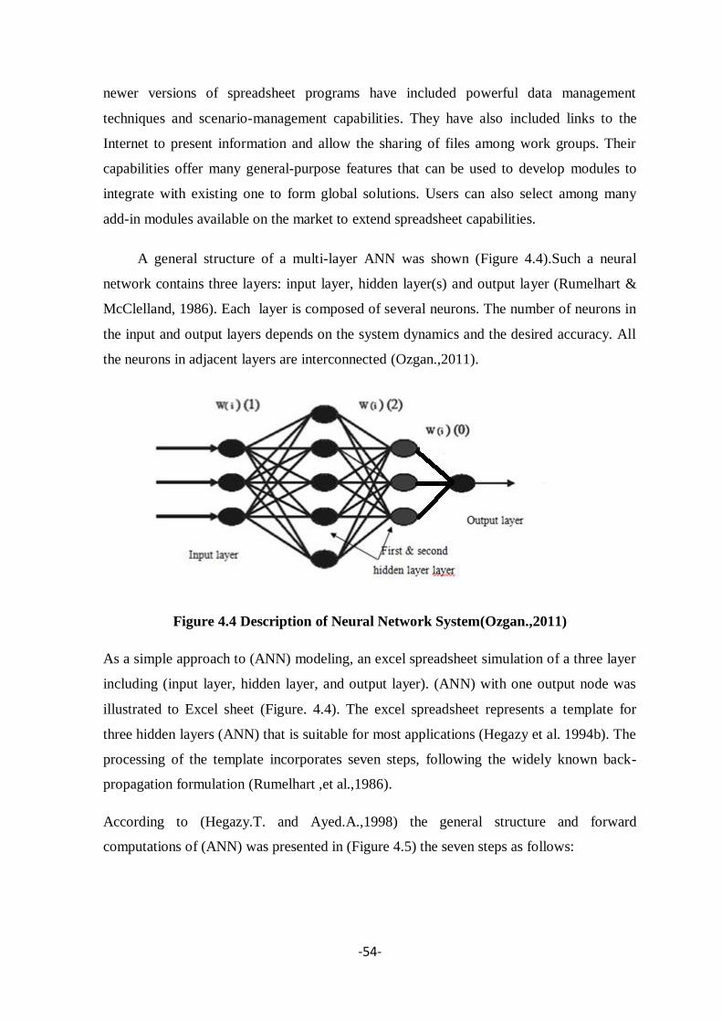
-54-
newer versions of spreadsheet programs have included powerful data management
techniques and scenario-management capabilities. They have also included links to the
Internet to present information and allow the sharing of files among work groups. Their
capabilities offer many general-purpose features that can be used to develop modules to
integrate with existing one to form global solutions. Users can also select among many
add-in modules available on the market to extend spreadsheet capabilities.
A general structure of a multi-layer ANN was shown (Figure 4.4).Such a neural
network contains three layers: input layer, hidden layer(s) and output layer (Rumelhart &
McClelland, 1986). Each layer is composed of several neurons. The number of neurons in
the input and output layers depends on the system dynamics and the desired accuracy. All
the neurons in adjacent layers are interconnected (Ozgan.,2011).
Figure 4.4 Description of Neural Network System(Ozgan.,2011)
As a simple approach to (ANN) modeling, an excel spreadsheet simulation of a three layer
including (input layer, hidden layer, and output layer). (ANN) with one output node was
illustrated to Excel sheet (Figure. 4.4). The excel spreadsheet represents a template for
three hidden layers (ANN) that is suitable for most applications (Hegazy et al. 1994b). The
processing of the template incorporates seven steps, following the widely known back-
propagation formulation (Rumelhart ,et al.,1986).
According to (Hegazy.T. and Ayed.A.,1998) the general structure and forward
computations of (ANN) was presented in (Figure 4.5) the seven steps as follows:

-55-
Figure 4.5: Spread Sheet Simulation of Three-Layer NN with One Output
Node(Hegazy.T. and Ayed.A.,1998).

-56-
Step 1. Data Organization , through this process, as a preliminary stage to ANN modeling,
we collect data from extraction and Marshall tests from different locations (BaniSwef-
ElMinya - Assyutfree way Project) and two different layers (binder and wearing) to make
a variety data in the spreadsheet which it will be appear in accuracy of the model results.
The data is first collected from extraction and gradation tests (sieve numbers and bitumen
content) and organized in rows, then we got the corresponding Marshall test (stability, flow
and air void ratio) but each of them putted in a different sheet with the same corresponding
(sieve numbers and bitumen content).for each variable (Figure 4.6), the minimum and
maximum values were also put in spreadsheet formulas to be used in step 2.
Step 2. Data Scaling, in this step, the input data part of the first matrix is scaled to a range
from [-1 to 1] to suit (ANN) processing. It was computed by constructing the second
matrix with linear formula for scaling the values of the first matrix (Hegazy.T. and
Ayed.A.,1998)., as follows:
2 x (Unscaled Value – Column Min.)
Scaled Value = -1 (1)
(Column Max.– Column Min.)
This scaling formula is written only one cell, and then copied to all cells in the scaling
matrix(Figure 4.7).
Step 3. Weight matrix (W), the third step to construct and initialize the weight matrix
between the inputs and the hidden layers. All inputs were fully connected to the hidden
nodes. All the values of the in weight matrix are considered variables to be determined in
(ANN) modeling (Figure 4.8). Through preliminary experimentation, it was found that
setting the initial weight values to a range (0.5 to 1) is appropriate for inputs scaled to a
range (-1 to 1) (Hegazy.T. and Ayed.A.,1998).
Step 4. Output of Hidden Nodes, this step is to allow the hidden nodes to process the input
data and produce values to be forwarded to the next layer. According to (ANN) processing
(Figure 1), each hidden node j receives activation Xj, which is sumproduct formula of
scaled inputs by their associated connection weights. Accordingly, each hidden node
produces an output Xjj that is a function of its activation, as follows:

-57-
Tanh function has shown the best results (Hegazy.T. and Ayed.A.,1998) As shown in Step
4 of (Figure 4.5), a formula was written for the first row of all hidden nodes and then
copied to the down cells(Figure 4.9).
Step 5. Weight Matrix (W`), similar to the weight matrix constructed in step 3, a second
matrix was constructed to connect the (L) hidden to the single output node.
These weights are additional variables in the model and were initialized as previously
described (Figure 4.10).
Step 6. Finally (ANN) Output, similar to step 4, the output of the (ANN) is computed by
calculating the sum product (Y) of each hidden node by its connection weight and then
processing this value through the tanh function as follows(Figure 4.11):
Step 7. Scaling Back (ANN) Output and Calculating the Error, in this step, the ANN
output is scaled back to the original range of values using the reverse of equation (1)
(Hegazy and Ayed el al.1998) as follows:
(Output Value + 1)x(Max. Output – Min. Output)
OutputScaled back = (6)
2
Output of ANN =tanh (Xj) (5)
L
Y =∑ (Xjj x Wjj) (4) J=1
Xjj =tanh (Xj) (3)
Xj =∑ (XjxWjj) (2)J=1

-58-
To calculate a measure of the (ANN) performance, a column is constructed for determining
the error between the actual outputs and (ANN) outputs as follows:
(ANN OUTPUT – ACTUAL OUTPUT)
ESTIMATING ERROR (%) = X 100 (7)
ACTUAL OUTPUT
It is also possible in the (ANN) simulation to use some cases for training and others for
testing. The average error of each group of cases can be calculated in a different cell and
then combined in a cell that calculates the performance measure of the (ANN), for
example:
Weighted Error (%)
= 0.5 (Test Average Error) + 0.5(Training Average Error) (8)
Where weight of 0.5 were assumed for illustration. This approach gives more emphasis to
the test cases which are usually a small numbers compared to training cases, to ensure
good performance and avoid overtraining (Hegazy.T. and Ayed.A.,1998).
4.6 Neural Network Implementation
Relevant data from job mix and quality control tests for the (Bani Swef-ElMinya –
Assyut free way Project) were collected and organized in a four spread sheets (Figure 4.6),
Sieve aggregate analysis and bitumen content corresponding to specimen
stability.
Sieve aggregate analysis and bitumen content corresponding to specimen
Flow.
Sieve aggregate analysis and bitumen content corresponding to specimen Air
Void and
Sieve aggregate analysis and bitumen content corresponding to specimen
Density.
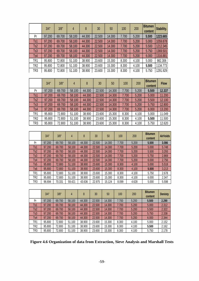
-59-
Figure 4.6 Organization of data from Extraction, Sieve Analysis and Marshall Tests
3/4'' 3/8'' 4 8 30 50 100 200Bitumen
contentStability.
Pr 97.200 69.700 58.100 44.300 22.500 14.300 7.700 5.200 5.500 1223.665
Ts1 97.200 69.700 58.100 44.300 22.500 14.300 7.700 5.200 5.000 1059.878
Ts2 97.200 69.700 58.100 44.300 22.500 14.300 7.700 5.200 5.500 1212.345
Ts3 97.200 69.700 58.100 44.300 22.500 14.300 7.700 5.200 5.750 1369.501
Ts4 97.200 69.700 58.100 44.300 22.500 14.300 7.700 5.200 6.000 1316.881
TR1 95.800 72.800 51.100 38.900 23.600 15.300 8.300 4.100 5.000 982.306
TR2 95.800 72.800 51.100 38.900 23.600 15.300 8.300 4.100 5.500 1134.773
TR3 95.800 72.800 51.100 38.900 23.600 15.300 8.300 4.100 5.750 1291.929
TR4 95.800 72.800 51.100 38.900 23.600 15.300 8.300 4.100 6.000 1239.309
TR5 96.694 70.331 59.421 43.636 22.975 15.124 8.099 4.628 5.000 1016.332
TR6 96.694 70.331 59.421 43.636 22.975 15.124 8.099 4.628 5.500 1168.799
TR7 96.694 70.331 59.421 43.636 22.975 15.124 8.099 4.628 5.750 1325.955
TR8 96.694 70.331 59.421 43.636 22.975 15.124 8.099 4.628 6.000 1273.335
3/4'' 3/8'' 4 8 30 50 100 200Bitumen
contentFlow
Pr 97.200 69.700 58.100 44.300 22.500 14.300 7.700 5.200 5.500 12.337
Ts1 97.200 69.700 58.100 44.300 22.500 14.300 7.700 5.200 5.000 11.200
Ts2 97.200 69.700 58.100 44.300 22.500 14.300 7.700 5.200 5.500 12.100
Ts3 97.200 69.700 58.100 44.300 22.500 14.300 7.700 5.200 5.750 12.800
Ts4 97.200 69.700 58.100 44.300 22.500 14.300 7.700 5.200 6.000 13.200
TR1 95.800 72.800 51.100 38.900 23.600 15.300 8.300 4.100 5.000 11.049
TR2 95.800 72.800 51.100 38.900 23.600 15.300 8.300 4.100 5.500 11.500
TR3 95.800 72.800 51.100 38.900 23.600 15.300 8.300 4.100 5.750 12.620
3/4'' 3/8'' 4 8 30 50 100 200Bitumen
contentAirVoids
Pr 97.200 69.700 58.100 44.300 22.500 14.300 7.700 5.200 5.500 3.086
Ts1 97.200 69.700 58.100 44.300 22.500 14.300 7.700 5.200 5.000 5.748
Ts2 97.200 69.700 58.100 44.300 22.500 14.300 7.700 5.200 5.500 3.293
Ts3 97.200 69.700 58.100 44.300 22.500 14.300 7.700 5.200 5.750 2.869
Ts4 97.200 69.700 58.100 44.300 22.500 14.300 7.700 5.200 6.000 2.756
Ts5 95.800 72.800 51.100 38.900 23.600 15.300 8.300 4.100 5.000 5.518
Ts6 95.800 72.800 51.100 38.900 23.600 15.300 8.300 4.100 5.500 3.213
TR1 95.800 72.800 51.100 38.900 23.600 15.300 8.300 4.100 5.750 2.678
TR2 95.800 72.800 51.100 38.900 23.600 15.300 8.300 4.100 6.000 2.347
TR3 96.694 70.331 59.421 43.636 22.975 15.124 8.099 4.628 5.000 5.598
3/4'' 3/8'' 4 8 30 50 100 200Bitumen
contentDenisty
Pr 97.200 69.700 58.100 44.300 22.500 14.300 7.700 5.200 5.500 2.290
Ts1 97.200 69.700 58.100 44.300 22.500 14.300 7.700 5.200 5.000 2.312
Ts2 97.200 69.700 58.100 44.300 22.500 14.300 7.700 5.200 5.500 2.322
Ts3 97.200 69.700 58.100 44.300 22.500 14.300 7.700 5.200 5.750 2.338
Ts4 97.200 69.700 58.100 44.300 22.500 14.300 7.700 5.200 6.000 2.344
TR1 95.800 72.800 51.100 38.900 23.600 15.300 8.300 4.100 5.000 2.152
TR2 95.800 72.800 51.100 38.900 23.600 15.300 8.300 4.100 5.500 2.162
TR3 95.800 72.800 51.100 38.900 23.600 15.300 8.300 4.100 5.750 2.178

-60-
Figure 4.7 Scaling of data
Figure 4.8 Weights of 5 hidden neurons
Figure 4.9 Outputs of hidden neurons
Figure 4.10 Weights of 5 hidden neurons to 1 output
3/4'' 3/8'' 4 8 30 50 100 200Bitumen
contentStability.
Pr 1.000 -0.621 0.758 1.000 -1.000 -0.250 -1.000 1.000 0.000 0.198
Ts1 1.000 -0.621 0.758 1.000 -1.000 -0.250 -1.000 1.000 -1.000 -0.615
Ts2 1.000 -0.621 0.758 1.000 -1.000 -0.250 -1.000 1.000 0.000 0.142
Ts3 1.000 -0.621 0.758 1.000 -1.000 -0.250 -1.000 1.000 0.500 0.922
Ts4 1.000 -0.621 0.758 1.000 -1.000 -0.250 -1.000 1.000 1.000 0.661
TR1 -0.556 0.471 -0.524 -0.421 0.001 1.000 0.122 -1.000 -1.000 -1.000
TR2 -0.556 0.471 -0.524 -0.421 0.001 1.000 0.122 -1.000 0.000 -0.243
TR3 -0.556 0.471 -0.524 -0.421 0.001 1.000 0.122 -1.000 0.500 0.537
3/4'' 3/8'' 4 8 30 50 100 200Bitumen
content
HN1 9.63E+09 2.11E+08 -2.2E+09 -1E+09 -1.6E+09 -1.5E+09 -1.2E+09 -3.8E+09 3.04E+09
HN2 -1.6E+09 1.58E+09 8.26E+09 6.09E+08 1.61E+09 3.39E+08 -1.4E+09 4.74E+09 9.13E+09
HN3 -5.9E+09 1.18E+09 7.05E+08 8.19E+08 -3E+07 -5E+08 -3.2E+07 2.23E+09 7.5E+09
HN4 -6.3E+08 -9.8E+09 2.18E+09 -2.5E+09 -9.6E+08 -2E+09 -1.6E+09 4.96E+08 -7.9E+07
HN5 -2.2E+08 -2.9E+08 -1.4E+08 -1E+10 -5.5E+08 2.06E+09 6E+09 -5.9E+08 -9.4E+09
HN1 HN2 HN3 HN4 HN5
Pr 1 1 -1 1 -1
Ts1 1 -1 -1 1 -1
Ts2 1 1 -1 1 -1
Ts3 1 1 1 1 -1
Ts4 1 1 1 1 -1
TR1 -1 -1 -1 -1 1
TR2 -1 -1 1 -1 1
TR3 1 -1 1 -1 1
HN1 HN2 HN3 HN4 HN5
HN22 0.332943 0.414857 0.72081 0.582095 0.408374

-61-
Figure 4.11 Neural network Output
Figure 4.12 Scaling back and calculating the error
4.7 Determining NN Weights
Once the Excel spreadsheet has been set up with initial weights of [0 to 1], it was
apparent that overall performance indicator of cell (I 195) (Figure 4.13) showing a very
high error value. Because all formulas in the template are functions of the weights, the next
step was to determine the (ANN) weight values that would optimize (ANN) performance.
In this thesis genetic algorithm (GA) technique using Evolver 5.5 optimization add-in for
Microsoft Excel software from Palisade Corporation was used. The details of (GA) are
provided as follow:
Pr 0.198059
Ts1 -0.55737
Ts2 0.198059
Ts3 0.927798
Ts4 0.927798
Ts5 -0.9278
Ts6 -0.19806
TR1 0.434292
TR2 0.444754
TR3 -0.44475
NN output
% Errors
Pr 1223.665 Pr
Ts1 1071.478 Ts1 1059.88 1.09
Ts2 1223.665 Ts2 1212.34 0.93
Ts3 1370.678 Ts4 1369.50 0.09
Ts4 1370.678 Ts5 1316.88 4.09
Ts5 996.8517 Ts6 982.31 1.48
Ts6 1143.864 Ts7 1134.77 0.80
TR1 1271.257 Ts8 1291.93 1.60
TR2 1273.364 TR1 1239.31 2.75
TR3 1094.165 TR2 1016.33 7.66
Actual Stability.NN output Scaled
back
-62-
Figure 4.13 (ANN) Templates
4.7.1 Genetic Algorithm (GA) technique
This technique is fundamentally different from traditional simplex based algorithms
such as the one used by Excel Solver. It uses the method of evolution, specifically survival
of the fittest. The theory behind (GA) is that a population of a certain species will, after
many generations of random evolution, adapt to live better in its environment. (GA) solved
optimization problems in the same fashion. First, a population of possible solutions to the
problem is created. Individuals in the population are then allowed to randomly breed, a
process called crossover, until the fittest offspring (the one that solves the problems best) is
generated. After a large number of generations, a population eventually emerges wherein
the individuals will provide an optimum or close to optimum solution (Hegazy.T. and
Ayed.A.,1998).
4.7.2 Evolver
For the case study at hand, commercial (GA) software (Evolver5.5 optimization) was
used to find the optimum originals weights at step 3 and step 5 (Figure 4.14) of the model.
Since, the training of the back-propagation network is performed by Evolver, a brief
description about the software and the data input is given below.

-63-
Evolver uses a proprietary set of genetic algorithms to search for optimum solutions to a
problem, along with probability distributions and simulation to handle the uncertainty
present in model. Genetic algorithms are used in Evolver to find the best solution for
model.
Figure 4.14 Original Weights of the Spread Sheets
Genetic algorithms mimic Darwinian principles of natural selection by creating an
environment where hundreds of possible solutions to a problem can compete with one
another, and only the “fittest” survive. Just as in biological evolution, each solution can
pass along its good “genes” through “offspring” solutions so that the entire population of
solutions will continue to evolve better solutions. The terminology used when working
with genetic algorithms is often similar to that of its inspiration. Crossover functions help
focus the search for solutions, “mutation” rates help diversify the “gene pool”, and
evaluate the entire “population” of solutions or “organisms”. (Cell I 154) representing the
(ANN) training weighted error was selected to be minimized. The screen model definition
at Evolver adjustable cells ranges (Figure.4.15) containing the optimization variables were
also specified as the two weight matrices. Adjustable cells founded that the range from (-
1000000 to 1000000) gives satisfied results, at the same screen constraints was founded
from (0 to 10) for testing trials and (0 to 15) for training trials.
At setting screen (Figure4.16) after many trials it was founded that 100000 trials and
progress maximum change 0.01% with number of trials 5000 give acceptable results.
During the (GA) optimization, Evolver options can be used to enhance the results. For
example, population size affects processing time because the fitness function must be

-64-
calculated for every individual in every generation. A population size 50 was found as a
good number to start with. The number can be increased later during the optimization
process. Chromosome length presents the level of accuracy needed for the adjustable cells.
Figure 4.15 Evolver Model Definition Screen
Figure 4.16 Evolver Optimization Setting Screen

-65-
Appendix C shows the sample report of optimization process using Evolver, the report was
appeared automatically after the end of optimization process in a single sheet.
The most remarkable results in this report are no. of valid trials, no. of total trials, original
value, best value found, reason optimization stop and total optimization time.
4.8 Comparing experimental results with the ANN model
The Marshall Test Results data (Stability, Flow, Air Void, and Density) were
presented on charts (Figures 4.17- 4.20) shows the big different between experimental and
predicted results before Genetic Algorithm running.
Furthermore, the results comparison by the error percentage is the main focus and can be
computed by
Error% =Absolute ((experimental – Predicted)/experimental)*100
After the end of the optimization process at each sheet it founded that difference
chart between the experimental and predicted results error was minimized. (Figures from.
4.17 to 4.20) show this.
Comparison of the results yields that Evolver is effective in modeling the problem
and its predictions’ is close to real data.
If the previous recorded data (input data) increase, the error percentage decrease and more
accurate Marshall Test results (output data) will be gained.
4.9 Analysis
4.9.1 Average Error
After the ANN model has been developed, it seems in (Figure.4.21) that the
weighted error in all Marshall Results was acceptable; it had maximum error not exceed
3.99% at stability, 2.38% at flow, 9.46%at air voids and 2.41%at density.

-66-
Figure 4.17.a Stability Before Optimization.
Figure 4.17.b Stability After Optimization.
Experiments
Mar
shal
l S
tabil
ity (
kg)
Experiments
Mar
shal
l S
tabil
ity (
kg)

-67-
Figure 4.18.a Flow Before Optimization.
Figure 4.18.b Flow After Optimization.
Experiments
Experiments
Flo
w V
alue
in 0
.0 1
/ in
F
low
Val
ue
in 0
.0 1
/ in

-68-
Figure 4.19.a Air Void Before Optimization.
Figure 4.19.b Air Void After Optimization.
Experiments
Experiments
Air
Void
s %
A
ir V
oid
s %

-69-
Figure 4.20.a Density Before Optimization.
Figure 4.20.b Density After Optimization.
Experiments
Experiments
Unit
Wei
ght
g/c
m3
Unit
Wei
ght
g/c
m3

-70-
Figure 4.21 The ANN Model After Developed Error

-71-
4.9.2 Detailed Error analysis
A detailed error analysis was also performed and is shown in (Figure 4.21.a, b, c, d),
which illustrates the error distribution for both the training and testing cases.
As shown for table (4.1) training error percentage, more than 55.77% less than 3 %,
14.43% between 5-7%, 17.3% between 5-7% and less than 1% between 7 – 10 %
As shown for table (4.1) testing error percentage, more than 58.35% less than 3 %, 21.79%
between 5-7%, 3.845% between 5-7% and less than 1% between 7 – 10 %
Table 4.1 Summary of Training and Testing Error
Training
Error % Stability Flow Air voids Density Average
0-3% 42.31 73.08 19.23 88.46 55.77
3-5% 26.92 19.23 7.69 3.85 14.43
5-7% 26.92 7.69 26.92 7.69 17.3
7-10% 3.85 0 0 0 0.925
Testing
Error % Stability Flow Air voids Density Average
0-3% 83.33 66.67 16.67 66.67 58.35
3-5% 16.67 33.33 3.85 33.33 21.79
5-7% 0 0 15.38 0 3.845
7-10% 0 0 0 0 0

-72-
Figure 4.22.a Error distribution, Training and Testing sets
Error %
Error %
% o
f ex
per
imen
ts
% o
f ex
per
imen
ts
-73-
Figure 4.22.b Error distribution, Training and Testing sets
Error %
% o
f ex
per
imen
ts
Error %
% o
f ex
per
imen
ts
-74-
Figure 4.22.c Error distribution, Training and Testing sets
Error %
% o
f ex
per
imen
ts
Error %
% o
f ex
per
imen
ts

-75-
Figure 4.22.d Error distribution, Training and Testing sets
% o
f ex
per
imen
ts
% o
f ex
per
imen
ts
Error %
Error %

-76-
4.10 Validating of the model
Once the ANN model has been developed, it can be put to actual new sieve and
bitumen percentages use in predicting the Marshall Results for new (HMA).(Figure 4.23)
shows estimation screen for new (HMA), Marshall Results (stability, flow, air voids and
density) linked to previous ANN models individually.
Figure 4.23 Estimation Screen for New Marshall Results
Data collected from another two projects to validate the model, sixteen experiments
from ”Orascome Company” and fourteen experiments from the ”General Nile Company”,
Table 4.2 illustrated maximum and minimum pass sieve percentage and Marshall Test
results data from two projects.
Table 4.2 The Characteristics of HMA
Test
Project 1 Project 2
Minimum
Value
Maximum
Value
Minimum
Value
Maximum
Value
Extraction Test
%passing from sieve 1”
%passing from sieve 3/4”
%passing from sieve 3/8”
100
94.29
54.76
100
98.09
60.48
100
93.1
70
100
96.4
77.5

-77-
%passing from sieve no .4
%passing from sieve no .8
%passing from sieve no .30
%passing from sieve no .50
%passing from sieve no .100
%passing from sieve no .200
% of bitumen content
Marshall Test
Marshall Stability (kg)
Marshall Flow (1/100 inch)
Air void ratio
Density (gm/cm3)
36.07
25.21
9.88
6.75
4.77
2
4.4
1107.7
11.3
6.39
2.25
39.75
28.29
11.89
7.83
5.71
2.96
4.7
1265.73
12.53
6.9
2.3
48.5
35.8
20.5
13.4
7.4
3.2
5.22
1208.2
10.8
2.83
2.34
51.1
38.9
25.2
15.9
8.3
4.1
5.36
1321.2
11.6
4.8
2.61
Previous experiments inserted to the Estimation screen to predict the results, (Figure 4.24)
shows the percentage of average error after using the model to predict Marshall Test results
data, following equations 1&2 show calculations of the average error.
𝑬𝒔𝒕𝒊𝒎𝒂𝒕𝒊𝒏𝒈 𝑬𝒓𝒓𝒐𝒓 (%) = 𝑨𝑵𝑵 𝑶𝑼𝑻𝑷𝑼𝑻 − 𝑨𝒄𝒕𝒖𝒂𝒍 𝑶𝒖𝒕𝒑𝒖𝒕
𝑨𝒄𝒕𝒖𝒂𝒍 𝑶𝒖𝒕𝒑𝒖𝒕× 𝟏𝟎𝟎
𝑨𝒗𝒆𝒓𝒂𝒈𝒆 𝑬𝑹𝑹𝑶𝑹 = 𝑬𝒔𝒕𝒊𝒎𝒂𝒕𝒊𝒏𝒈 𝑬𝒓𝒓𝒐𝒓𝒏
𝒊=𝟏
𝒏
Where n is number of experiments.

-78-
Figure 4.24 The Percentage of Error of Projects
900
1000
1100
1200
1300
1400
1500
1600
1 3 5 7 9 11 13 15 17 19 21 23 25 27 29
Stability
observed
predictedAverageError =1.76%
8
9
10
11
12
13
14
15
16
1 3 5 7 9 11 13 15 17 19 21 23 25 27 29
Flow
Observed
PredictedAverageError =3.72%
Mar
shal
l S
tabil
ity (
kg)
Experiments
Flo
w V
alue
in 0
.0 /
in
Experiments

-79-
Figure 4.24 The Percentage of Error of Projects (cont.)
2
3
4
5
6
7
8
9
10
11
121 3 5 7 9
11 13 15 17 19 21 23 25 27
Air Voids
Observed
Predicted
AverageError =3.96%
0.5
1
1.5
2
2.5
3
3.5
4
1 3 5 7 9
11 13 15 17 19 21 23 25 27 29
Density
Series1
Series2AverageError =2.27%
Experiments
Experiments
Air
Void
s %
U
nit
Wei
ght
g/c
m3

-80-
4.11 Summary
This chapter demonstrates the seven steps ANN model with two hidden layers using
Microsoft Excel were suitable for organization of data.
Genetic Algorithm commercial software (Evolver 5.5) used to detect the suitable weights
of hidden layers. Detailed error analysis shown in (table 4.1) illustrated it were acceptable.
The proposed model is valid among the ranges (maximum and minimum values) of the
previously recorded experimental database which illustrated in (table 3.7) to predict a
future Marshall Test results.
The model validated by thirty experiments goes between ranges and the errors were
acceptable (Figure 4.25).
Figure 4.25 Error percentage of validating experiments
1.76%
3.72%3.96%
2.27%
0.00%
0.50%
1.00%
1.50%
2.00%
2.50%
3.00%
3.50%
4.00%
4.50%
Average Error
Stability Flow Air Voids Density

-81-
Chapter Five
CONCLUSION AND RECOMMENDATIONS
-82-
Chapter 5
CONCLUSION AND RECOMMENDATIONS
5.1 Introduction
The thesis is presented in five chapters encircling the whole research; this chapter
reveals the summary of the study, also the chapter cites the appropriate current
recommendations, which the researcher developed based on the research study.
The Extract, Sieve Analysis and Marshall Tests recorded data are the most important
tests to control the quality in any pavement projects according to the quality control
specifications of these projects.
The study demonstrates the benefits of using Artificial Neural Network technique for
prediction of future depends on previous recorded data. thesis presents a model to predict
Marshall Test Results depending on Extract and Sieve Analysis Test data. Modeling the
Marshall Test Results of (HMA) is very important in quality control process without
carrying out destructive tests which takes too much time and human effort.
The structure of a simple Artificial Neural Network (ANN) was simulated using a
spreadsheet program (Excel) to provide a transparent and simplified representation of this
technique.
Genetic Algorithm commercial software (Evolver 5.5) used to optimize the weights of
(ANN) then to get a reasonable percentage error results.
The model allows the user to input sieve size passing percentage from sieve analysis test
and bitumen content from extraction test then automatically get the Marshall Test results.
5.2 Conclusion
Based on the results of the developed models and from the experiences gained in this
work it was concluded that:
Using same kind of (HMA) (wearing, binder….etc.) to predict Marshall Test results
at the (ANN) model give more accurate results.

-83-
It founded that there is a great effect of percentage of bitumen in (HMA)
characteristic especially in stability.
The proposed model is valid for the ranges of the experimental database which it
was shown at (table 3.7) used for (ANN) modeling.
The Marshall Test results of the (HMA) was nonlinear, the proposed (ANN)
method had the ability to model it. The ability of (ANN) method to model
nonlinear data indicates that the model can also be used for hot mix asphalt designs.
5.3 Recommendations
First of all, the compilation, evaluation, and accuracy of historical data demanded for
the development of the future Marshall Test results prediction models represents the most
critical part of the research work.
The following recommendations will be useful to develop the model in the future.
Increasing input trials data especially experimental Marshall Test with different
percentage of bitumen and sieve passing will reduce the error of the model.
In the future new factors like (temperature, kind of aggregate, characteristics of
bitumen …etc) need to be inserted to the model to improve the predication
process.
Using microprogramming to enhance the interface of Microsoft Excel will be
useful
Using the model to predict pass sieve percentage dependent on Marshall Test
characteristics which the project need.

-84-
REFERENCES
Aasadullah. Attal (2010). Development of Neural Network Models for Prediction of
Highway Construction Cost and Project Duration. Civil Engineering, Ohio
University. Master of Science: 145.
AASHTO-T245 (2006). Standard Method of Test for Resistance to Plastic Flow of
Bituminous Mixtures Using Marshall Apparatus, American Association of
State Highway and Transportation Officials.
AASHTO-T-27 (2006). Standard method of test for sieve analysis of fine and coarse
aggregates. Washington, D.C., American Association of State Highway and
Transportation Officials.
Adeli, Hojjat and K. A (2001). Construction scheduling, cost optimization, and
management : a new model based on neurocomputing and object technologies.
London; New York, Spon Press.
Adeli, H. and M. Y. Wu (1998). "Regularization neural network for construction cost
estimation." Journal of Construction Engineering and Management-Asce
124(1): 18-24.
Alsugair, A. M. and A. A. Al-Qudrah (1998). "Artificial neural network approach for
pavement maintenance." Journal of Computing in Civil Engineering.ASCE,
12(4): 249-255.
ASTM-D2127 Method of Test for Bitumen Content of Paving Mixtures by Centrifuge
(Withdrawn 1964).
Attoh-Okine, N. O. (2001). "Grouping pavement condition variables for performance
modeling using self-organizing maps." Computer-Aided Civil and
Infrastructure Engineering 16(2): 112-125.
Belli, M. R., M. Conti, Crippa, P and C. Turchetti (1999). "Artificial neural networks
as approximators of stochastic processes." Neural Networks 12(45): 647-658.
Bosurgi, G. and F. Trifiro (2005). "A model based on artificial neural networks and
genetic algorithms for pavement maintenance management." The
International Journal of Pavement Engineering 6(3): 201-209.
Bruen, M. and J. Q. Yang (2005). "Functional networks in real-time flood forecasting
- a novel application." Advances in Water Resources 28(9): 899-909.
Cal, Y. (1995). "Soil classification by neural network." Advances in Engineering
Software, 22: 95-97.
Ceylan, H., A. Guclu, E. Tutumluer and M. R. Thompson (2005). "Backcalculation of
full-depth asphalt pavement layer moduli considering nonlinear
stressdependent subgrade behavior." The International Journal of Pavement
Engineering, 6(3): 171-182.
Chao, L. and M. Skibniewski (1994). "Estmating construction productivity- neural –
network-based approach." Journal of Computing in Civil Engineering 8(2):
234-251.

-85-
Chao, L. C. and M. Skibniewski (1995). "Neural-network method of estimating
construction technology acceptability." Journal of Construction Engineering
and Management-Asce, 121(1): 130-142.
Cheng, M. Y., H. C. Tsai and W. S. Hsieh (2009). "Web-based conceptual cost
estimates for construction projects using Evolutionary Fuzzy Neural Inference
Model." Automation in Construction 18(2): 164-172.
Eldin, N. N., & Senouci, A. B (1995). "A pavement condition rating model using
backpropagation neural network." Microcomputers in Civil Engineering,
10(6): 433-441.
Ezeldin, A. S. and L. M. Sharara (2006). "Neural networks for estimating the
productivity of concreting activities." Journal of Construction Engineering
and Management-Asce, 132(6): 650-656.
Fletcher, G. P. and C. J. Hinde (1995). "Using neural networks as a tool for
constructing rule-based systems." Knowledge-Based Systems 8(4): 183 -189.
Flood and K. Worley (1995). "An artificial neural-network approach to discrete-
event simulation." Ai Edam-Artificial Intelligence for Engineering Design
Analysis and Manufacturing, 9(1): 37-49.
Flood, I. (2006). "Next generation artificial neural networks for civil engineering."
Journal of Computing in Civil Engineering 20(5): 305-307.
Gagarin, N., I. Flood and P. Albrecht (1994). "Computing truck attributes with
artificial neural networks." Journal of Computing in Civil Engineering, ASCE
8(2): 179-200.
Hegazy.T. and Ayed.A. (1998). "NEURAL NETWORK MODEL FOR
PARAMETRIC COST ESTIMATION OF
HIGHWAY PROJECTS." Journal of Construction Engineering and Management-
Asce 124(3).
instruments, n. e. (2014). "Bitumen Testing Instruments." from
http://www.newtechnolabinstruments.in/bitumen-testing-instruments.html.
Kadyali, L. R. and N. B. Lal (2008). Principles and Practices of Highway Engineering,
Khanna Publishers, New Delhi.
Khanfar and A. Kholoqui (2007). Feasibility of the use of two spent blast materials as
aggregate in hot mix asphalt in Louisiana post-Katrina, ProQuest.
Kim, G., H. Yoon, S. An, H. Cho and K. Kang (2004). "Neural network model
incorporating a genetic algorithm in estimating construction costs." Building
and Environment. 93(11): 1235-1242.
Kim, Y. and Y. R. Kim (1998). Prediction of layer moduli from FWD and surface
wave measurements using artificial neural network. transportation research
board, 77th annual meeting. Washington, DC, USA.
Lee, B. J. and H. D. Lee (2004). "Position-invariant neural network for digital
pavement crack analysis." Computer-Aided Civil and Infrastructure
Engineering . 19(2): 105-118.

-86-
Liu, L., K. Zhu and K. Zhu (2007). "Improving cost estimates of construction
projects using phased cost factors." Journal of Construction Engineering and
Management-Asce 133(1): 92-95.
Lowe, D. J., M. W. Emsley and A. Harding (2006). "Predicting construction cost
using multiple regression techniques." Journal of Construction Engineering
and Management-Asce, 132(7): 750-758.
Mathew, T. V. and K. Krishna Rao (2006). "Introduction to Transportation
engineering." Civil Engineering–Transportation Engineering. IIT Bombay,
NPTEL ONLINE, http://www. cdeep. iitb. ac. in/nptel/Civil% 20Engineering.
Mei, X., M. Gunaratne, J. J. Lu and B. Dietrich (2004). "Neural network for rapid
evaluation of shallow cracks in asphalt pavements." Computer-Aided Civil
and Infrastructure Engineering , 19(3): 223 - 230.
Mfg, H. (2014). "Centrifuge Extractor[online]." 2014, from
http://www.humboldtmfg.com/centrifuge_extractor_analog_control_explosion
_proof_2.html.
Moselhi, O., T. Hegazy and P. Fazio (1991). "Neural networks as tools in
construction." Journal of Construction Engineering and Management-Asce
117(4): 606-625.
Murtaza, M. B. and D. J. Fisher (1994). "Neuromodex – neural-network system for
modular construction decision-making." Journal of Computing in Civil
Engineering, 8(2): 221-223.
Owusu-Ababia, S. (1998). "Effect of neural network topology on flexible pavement
cracking prediction." Computer-Aided Civil and Infrastructure Engineering,
13(5): 349-355.
Ozgan., E. (2011). "Artificial neural network based modelling of the Marshall
Stability of asphalt concrete." Expert Systems with Applications 38(5): 6025-
6030.
Pickard, S. (1997). "Integrated spreadsheets." Civil Engineering. ASCE 67(6): 44-45.
Rafiq, M. Y., G. Bugmann and D. J. Easterbrook (2001). "Neural network design for
engineering applications." Computers & Structures 79(17): 1541-1552.
Rajasekaran, S., M. F. Febin and Ramasamy (1996). "Artificial fuzzy neural
networks in civil engineering." Computers & Structures, 61(2): 291-302.
Razaqpur, A. G., A. O. Abd El Halim and H. A. Mohamed (1996). "Bridge
management by dynamic programming and neural networks." Canadian
Journal of Civil Engineering, 23: 1064-1069.
Reed, R. D. and R. J. Marks (1998). Neural smighing:Supervised learning in
feedforward artificial neural networks. Mass combridge. Combridge.
Ritchie, S. G., M. Kaseko and B. Bavarian (1991). "Development of an intelligent
system for automated pavement evaluation." Transportation Research Record
1311: 112-119.
Roberts, C. A. and N. O. Attoh-Okine (1998). "A comparative analysis of two
artificial neural networks using pavement performance prediction."
Computer-Aided Civil and Infrastructure Engineering, 13(5): 339-348.
-87-
Rumelhart, D., G. Hinton and R. Williams (1986). Learning Internal Representations
by Error Propagation, Parallel Distributed Processing, Explorations in the
Microstructure of Cognition, ed. DE Rumelhart and J. McClelland. Vol. 1.
1986, MIT Press, Cambridge, MA.
Shekharan, A. R. (1998). Effect of noisy data on pavement performance prediction by
artificial neural networks. transportation research board, 77th annual
meeting. Washington, DC, USA.
Skitmore, R. M. and S. T. Ng (2003). "Forecast models for actual construction time
and cost." Building and Environment 38(8): 1075-1083.
Sodikov, J. (2005). "Cost estimation of highway projects in developing
countries." Journal of the Eastern Asia Society for Transportation Studies 6: 1036-
1047.
Sonmez , R. (2004). "Conceptual cost estimation of building projects with regression
analysis and neural networks." Canadian Journal of Civil Engineering 31(4):
677-683.
Sonmez, R. and J. E. Rowings (1998). "Construction labor productivity modeling
with neural networks." Journal of Construction Engineering and
Management-Asce 124(6): 498-504.
Tam, C. M., T. K. L. Tong, T. C. T. Lau and K. K. Chan (2004). "Diagnosis of
prestressed concrete pile defects using probabilistic neural networks."
Engineering Structures 26(8): 1155-1162.
Tapkın, S. (2004). A recommended neural trip distribution model. Civil Engineering
Department,, Middle East Technical University. PhD thesis.
Tutumluer, E. and U. Seyhan (1998). Neural network modeling of anistropic
aggregate behavior from repeated load triaxial tests. transportation research
board 77th annual meeting. Washington, DC, USA.
W., R. and Lenz. ( 2011). " Pavement Design Guide." from
http://onlinemanuals.txdot.gov/txdotmanuals/pdm/pavement_types.htm.
Wilmot, C. G. and B. Mei (2005). "Neural network modeling of highway construction
costs." Journal of Construction Engineering and Management-Asce 131(7):
765-771.
Young II, W. A., W. S. Holland and G. R. Weckman (2008). "Determining hall of
fame staute for major league baseball using an artificial neural network."
Journal of Quantitative Analysis in Sports 4(4): 1-44.
Zhang, G. P., B. E. Patuwo and M. Y. Hu (2001). "A simulation study of artificial
neural networks for nonlinear time-series forecasting." Computers &
Operations Research 28(4): 381-396.

-88-
Appendix A
8
#100 7.7 5.7 9.7 7 15
#200 5.2 4.2 6.2 3
23
#30 22.5 19.5 25.5 19 30
#50 14.3 12.3 16.3 13
50
#4 58.1 55.1 61.1 48 65
#8 44.3 41.3 47.3 35
80
90
100
"1/2 78.7 74.7 82.7 70
"3/8 69.7 65.7 73.7 60
"3/4 97.2 93.2 100 80
Upper Limit Lower Limit
100
El Minia - Assute free wayLab. Division
Bituminous Mix Design (wearing Course)25mm
Gradation of the proposal JMF wearing Course
100
Sieves No.
"1 100 100 100
JMF (Total)JMF tolerance
Limits of project technical
Specifications
Lower Limit Upper Limit
0
20
40
60
80
100
120
"1 "3/4 "1/2 "3/8 #4 #8 #30 #50 #100 #200
% o
f P
ass
ing
Sieves Size
JMF (Total)
Lower Limit
Upper Limit
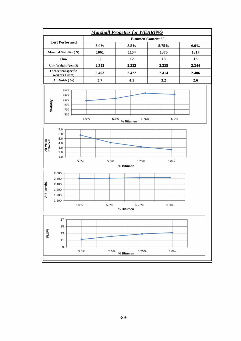
-89-
5.0% 5.5% 5.75% 6.0%
Marshal Stability ( N) 1061 1154 1370 1317
Flow 11 12 13 13
Unit Weight (g/cm3) 2.312 2.322 2.338 2.344
Theoretical specific
weight ( Gmm)2.453 2.422 2.414 2.406
Air Voids ( %) 5.7 4.1 3.2 2.6
bit
3
3.5
4
Marshall Propeties for WEARING
Test PerformedBitumen Content %
500
700
900
1100
1300
1500
5.0% 5.5% 5.75% 6.0%% Bitumen
Sta
bil
ity
1.0
2.0
3.0
4.0
5.0
6.0
7.0
5.0% 5.5% 5.75% 6.0%
% Bitumen
Air
Vo
ids
Reta
ine
d
1.500
1.700
1.900
2.100
2.300
2.500
5.0% 5.5% 5.75% 6.0%
% Bitumen
Un
it w
eig
ht
9
11
13
15
17
5.0% 5.5% 5.75% 6.0%% Bitumen
FL
OW

-90-
Appendix B

-91-

-92-
Appendix C
Optimization Summary Report
Evolver: Optimization Summary Performed By: keno
Date: 14 و10:52:41 2013, أثشيم
Model: ANN11.xlsx
Goal
Cell to Optimize Stability!$I$195
Type of Goal Minimum
Results
Valid Trials 100000
Total Trials 100000
Original Value 35.86
+ soft constraint penalties 0.00
= result 35.86
Best Value Found 3.99
+ soft constraint penalties 0.00
= result 3.99
Best Simulation Number 98702
Time to Find Best Value 0:33:10
Reason Optimization Stopped Number of trials
Time Optimization Started 14/04/2013 22:19
Time Optimization Finished 14/04/2013 22:52
Total Optimization Time 0:33:31
Adjustable Cell Values Stability!$E$96
Original 481227.0883
Best -667644.842
Adjustable Cell Values Stability!$F$96
Original 542696.0173
Best -1000000
Adjustable Cell Values Stability!$G$96
Original 471999.6587
Best -1000000
Adjustable Cell Values Stability!$H$96
Original 91688.2801
Best -1000000
Adjustable Cell Values Stability!$I$96
Original -84678.95351
Best -1000000
Adjustable Cell Values Stability!$J$96
Original -543506.6512
Best -1000000
Adjustable Cell Values Stability!$K$96
Original -401556.1278

-93-
Best 981596.817
Adjustable Cell Values Stability!$L$96
Original -695885.4026
Best -298226.386
Adjustable Cell Values Stability!$M$96
Original -654449.3884
Best -1000000
Adjustable Cell Values Stability!$E$97
Original -184507.5618
Best 1000000
Adjustable Cell Values Stability!$F$97
Original -850209.9263
Best -1000000
Adjustable Cell Values Stability!$G$97
Original -485474.0749
Best -270925.271
Adjustable Cell Values Stability!$H$97
Original 12171.50179
Best -738747.6289
Adjustable Cell Values Stability!$I$97
Original -276038.779
Best -1000000
Adjustable Cell Values Stability!$J$97
Original 292610.1537
Best -1000000
Adjustable Cell Values Stability!$K$97
Original -50952.10671
Best 652979.0966
Adjustable Cell Values Stability!$L$97
Original 464245.9601
Best -699619.6572
Adjustable Cell Values Stability!$M$97
Original 705731.1289
Best -1000000
Adjustable Cell Values Stability!$E$98
Original -412019.495
Best -197552.6021
Adjustable Cell Values Stability!$F$98
Original 931316.3775
Best 168056.6186
Adjustable Cell Values Stability!$G$98
Original 44429.67224
Best -110211.9856
Adjustable Cell Values Stability!$H$98
Original 211005.0608
Best -1000000
Adjustable Cell Values Stability!$I$98
Original 890810.9687
Best 891665.669
Adjustable Cell Values Stability!$J$98

-94-
Original 89329.35443
Best 71850.41648
Adjustable Cell Values Stability!$K$98
Original -527819.3597
Best 118080.121
Adjustable Cell Values Stability!$L$98
Original -30536.10942
Best 616137.7628
Adjustable Cell Values Stability!$M$98
Original 354764.8063
Best 849568.3371
Adjustable Cell Values Stability!$E$99
Original 648524.9662
Best -166361.7483
Adjustable Cell Values Stability!$F$99
Original 510350.7485
Best 532979.0609
Adjustable Cell Values Stability!$G$99
Original -308511.3307
Best 423463.349
Adjustable Cell Values Stability!$H$99
Original 751127.3864
Best 818826.4182
Adjustable Cell Values Stability!$I$99
Original 119375.4664
Best 408093.1355
Adjustable Cell Values Stability!$J$99
Original 541719.1019
Best -1000000
Adjustable Cell Values Stability!$K$99
Original -12960.20762
Best 102758.8273
Adjustable Cell Values Stability!$L$99
Original 466610.5678
Best 113449.3654
Adjustable Cell Values Stability!$M$99
Original -619005.9152
Best -704622.2875
Adjustable Cell Values Stability!$E$100
Original -175163.8372
Best 1000000
Adjustable Cell Values Stability!$F$100
Original 443258.0568
Best -1000000
Adjustable Cell Values Stability!$G$100
Original -100683.932
Best -794015.114
Adjustable Cell Values Stability!$H$100
Original -731720.5365
Best -416692.514

-95-
Adjustable Cell Values Stability!$I$100
Original -47382.96429
Best -1000000
Adjustable Cell Values Stability!$J$100
Original -347114.4203
Best -1000000
Adjustable Cell Values Stability!$K$100
Original 931986.8102
Best 826021.4979
Adjustable Cell Values Stability!$L$100
Original 119958.1937
Best 319783.3765
Adjustable Cell Values Stability!$M$100
Original -182259.7557
Best -1000000
Adjustable Cell Values Stability!$D$147
Original 0.332931478
Best 0.332931478
Adjustable Cell Values Stability!$E$147
Original 0.415717188
Best 0.415717188
Adjustable Cell Values Stability!$F$147
Original 0.722272087
Best 0.722272087
Adjustable Cell Values Stability!$G$147
Original 0.580635592
Best 0.580635592
Adjustable Cell Values Stability!$H$147
Original 0.406879122
Best 0.406879122
Adjustable Cells
Description
Solving Method Recipe
Mutation Rate 0.1
Crossover Rate 0.5
Cell Range -1000000 <= Stability!$E$96:$M$100 <= 1000000
Cell Range -1000000 <= Stability!$D$147:$H$147 <= 1000000
Operators (scores) Default parent selection (0.2249)
Default mutation (0.1109)
Default crossover (0.1738)
Default backtrack (0.2751)
Arithmetic crossover (0.0446)
Heuristic crossover (0.0064)
Cauchy mutation (0.0769)
Boundary mutation (0.0034)
Non-uniform mutation (0.0336)
Linear (0.0503)
Local search (0.0000)
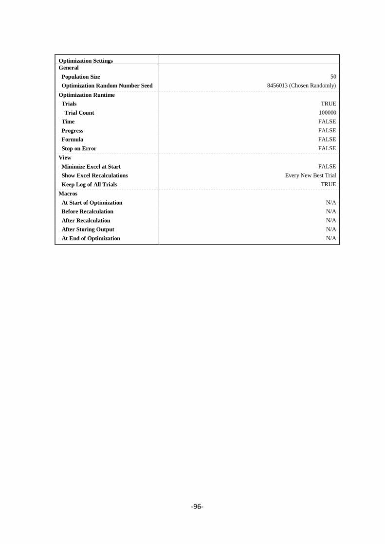
-96-
Optimization Settings
General
Population Size 50
Optimization Random Number Seed 8456013 (Chosen Randomly)
Optimization Runtime
Trials TRUE
Trial Count 100000
Time FALSE
Progress FALSE
Formula FALSE
Stop on Error FALSE
View
Minimize Excel at Start FALSE
Show Excel Recalculations Every New Best Trial
Keep Log of All Trials TRUE
Macros
At Start of Optimization N/A
Before Recalculation N/A
After Recalculation N/A
After Storing Output N/A
At End of Optimization N/A

-1-
يهخض انرسانة
انشطف االسفهت يعذ اهى و اشهش وسبئم انشطف ف يظش نزيع اشكبل انشطف سىاء ف انطشق او انطبساد او
ي % 3ان % 7ي انشكبو انتذسد وي % 97ان % 93يبطك االتظبس و تتكى انخهطخ االسفهتيخ تمشيجب ي
.انجيتىيي انسبخ
تعذ طشيمخ يبسشبل نتظيى انخهطخ االسفهتيخ ي اشهش انطشق انستخذيخ ثظش و تختض هز انطشيمخ ف تحذيذ
يكىبد انخهطخ االسفهتيخ ي انشكبو و سجخ انجيتىيي نتحميك انخىاص انطهىثخ نهخهطخ ي انخجبد و االسيبة و سجخ
انفشاغبد انهىائيخ و انكخبفخ و هز انتبئذ يتى انىطىل انيهب ثعذ ارشاء انعذيذ ي انتزبسة ثحتىيبد يختهفخ ي
هز انتبئذ تشتجط ثعاللخ غيشيجبششح ثعذح عىايم اههب تذسد , انجيتىيي ويتى استتبد انتبئذ ثطشيمخ انتزشثخ و انخطأ
.انشكبو و يحتىي انخهطخ االسفهتيخ ي انجيتىيي
ثعذ لجىل انخهطخ االسفهتيخ و احبء سيش انعم يتى ارشاء اختجبساد يبسشبل و االستخالص و انتذسد ف انىلع و انعم
دوسيب و رنك نمجىل انخهطخ وضجط انزىدح حيج يختض اختجبس يبسشبل ثمبسخ ست انخجبد و االسيبة و سجخ
انفشاغبد انهىائيخ و انكخبفخ ثبنخهطخ انتظييخ و االستخالص ف تحذيذ انسجخ انئىيخ نحتىي انجيتىيي ثبنخهطخ و
تتيض اختجبساد االستخالص و انتذسد ثسشعخ . يختض اختجبس انتذسد تحذيذ ست تىصيع احزبو انشكبو ثبنخهطخ
.ارشاءهب ف انىلع
انسىاد االخيشح اظهشد استخذايبد انشجكخ انعظجيخ االططبعيخ كبحذ اسبنيت انزكبء انظبع ف انهذسخ انذيخ
انهذف انرئيس ي انبحج هى استحذاث ىرج كجذيم نطشق انتىلعبد االعتيبديخ و اظهشد زبس يهحىظ و نزنك فب
و تذرج (تجربة االستخالص)قادر عه تىقع تائج تجربة يارشال انسانف ركرهى بذالنة سبة انبيتىيي ف انخهطة
.(تجربة انتذرج)انركاو
تى ثبنفعم تزيع تزبسة يبسشبل و تزبسة استخالص و تذسد ي عذح يشبسيع يفزح ثظش و عذح ششكبد يمبوالد
.وتى عم ىرد انشجكخ انعظجيخ االططبعيخ عه يهف اكسيم و اظهشد انتبئذ انهبئيخ سجخ خطأ طغيشح و يمجىنخ
يتى تزيع تزبسة عذيذح ي تزشثت انتذسد و االستخالص و انت يتى تفيز ثسشعخ سىاء ف انىلع او انعم و تزشثخ
يبسشبل نفس انخهطخ إلعذاد لبعذح ثيببد و سثطهى ثبنشجكخ انعظجيخ انظبعيخ و رنك نتىلع تبئذ تزشثخ يبسشبل
.انستمجهيخ ثذو ارشاءهب ثذالنخ تزشثت انتذسد و االستخالص
:تى تمسيى هز انشسبنخ ان خسخ فظىل كبالت
.يمذيخ تشم يهخض لظيش ع فكشح انشسبنخ واهذافهب و طشيمخ انعم: انفظم االول
تبسيخ االعبل انسبثمخ ثبنسجخ نهطشق و طشق انتظيى انختهفخ وانتشكيض عه طشيمخ تزشثخ : انفظم انخب
.يبسشبل و يمذيخ ع انشجكخ انعظجيخ انظبعيخ و استخذايبتهب
طشيمخ تزيع انعهىيبد ي تزبسة يبسشبل و انتذسد و االستخالص و تشتيجهب ف يهف : انفظم انخبنج
.ثشبيذ اكسيم

-2-
و يتحذث ع طشيمخ عم يهف االكسيم و استخذاو انشجكخ انعظجيخ انظبعيخ نتمهيم خطأ : انفظم انشاثع
.تىلع تبئذ تزشثخ يبسشبل ثذالنخ تزشثت انتذسد و االستخالص
.و يختض ثهخض انشسبنخ يع وضع يمتشحبد و تىطيبد نالعبل انستمجهيخ: انفظم انخبيس

االكاديية انعربية نهعهىو و انتكىنىجيا و انقم انبحري
كهية انهذسة و انتكىنىجيا
قسى هذسة انتشييذ و انباء
تىقع تائج تجربة يارشال باستخذاو انشبكة انعصبية انصاعية
اعذاد
عـــرو انقــــاوي جــعه
سسبنخ يمذيخ نالكبدييخ انعشثيخ نهعهىو و انتكىنىريب وانمم انجحشي إلستكبل يتطهجبد يم دسرخ
اناجستير
ف
انتشيذ و انباءهذسة
إشراف
و أكرو سهطا قطب.د.ا خانذ أىر قذيم. د.ا
قسى األشغال انعاية
هذسةكهية ال
قسى انتشييذ و انباء
هذسة كهية ال
جايعة عي شساالكاديية انعربية نهعهىو و انتكىنىجيا
و انقم انبحري
2014 ديسبر