Embed Size (px)
Citation preview
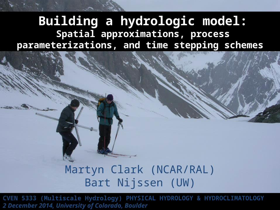
Martyn Clark (NCAR/RAL)Bart Nijssen (UW)
Building a hydrologic model:Spatial approximations, process parameterizations, and
time stepping schemes
CVEN 5333 (Multiscale Hydrology) PHYSICAL HYDROLOGY & HYDROCLIMATOLOGY2 December 2014, University of Colorado, Boulder
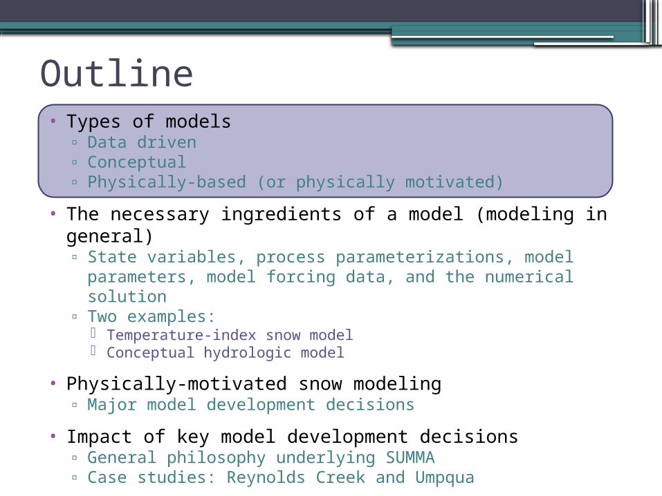
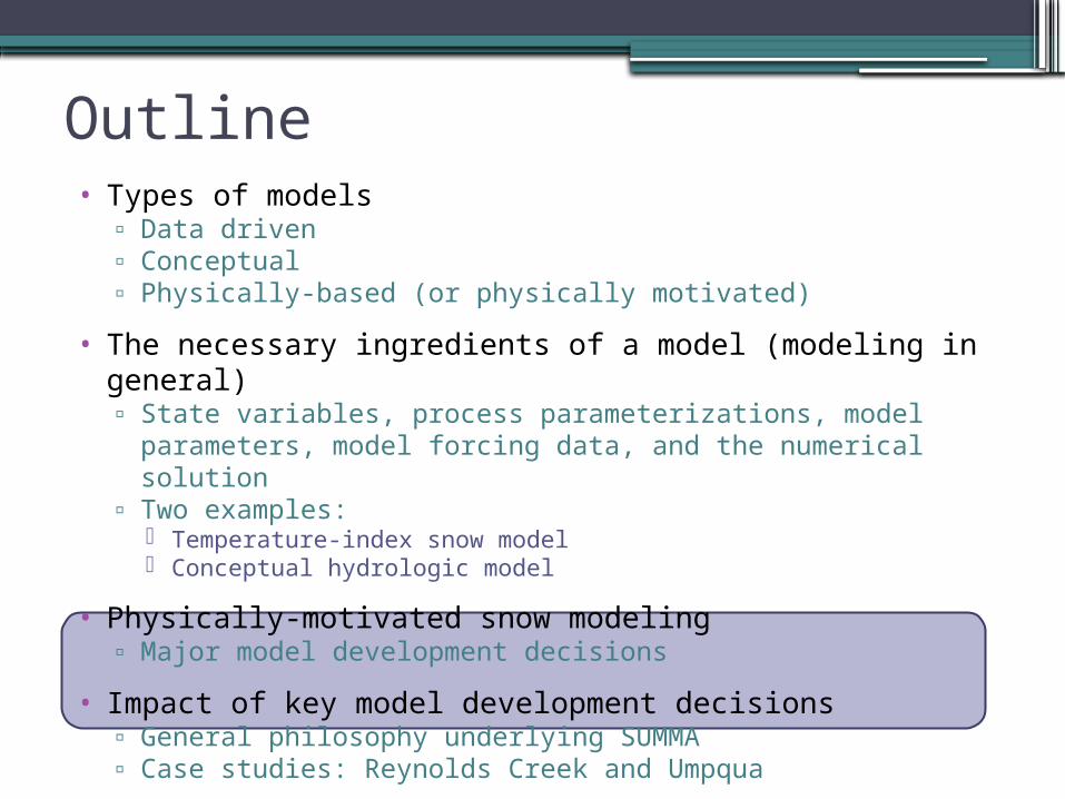
Outline• Types of models
▫ Data driven▫ Conceptual▫ Physically-based (or physically motivated)
• The necessary ingredients of a model (modeling in general)▫ State variables, process parameterizations, model parameters,
model forcing data, and the numerical solution▫ Two examples:
Temperature-index snow model Conceptual hydrologic model
• Physically-motivated snow modeling▫ Major model development decisions
• Impact of key model development decisions▫ General philosophy underlying SUMMA▫ Case studies: Reynolds Creek and Umpqua
• Summary and research needs
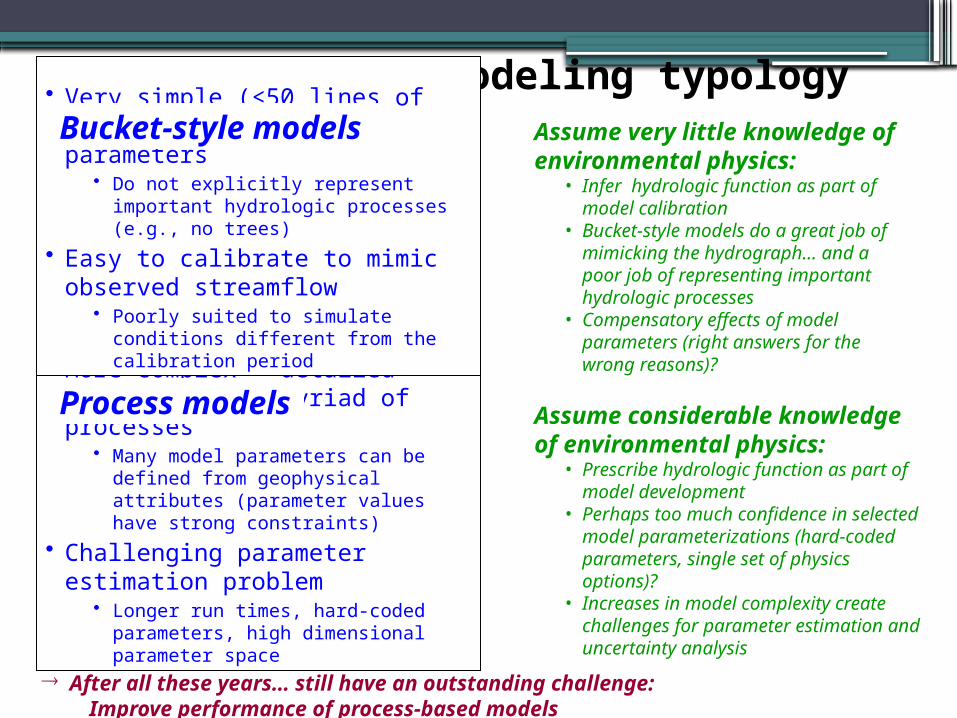
Assume very little knowledge of environmental physics:
• Infer hydrologic function as part of model calibration
• Bucket-style models do a great job of mimicking the hydrograph… and a poor job of representing important hydrologic processes
• Compensatory effects of model parameters (right answers for the wrong reasons)?
Basic hydrologic modeling typology
• More complex – detailed depiction of a myriad of processes
• Many model parameters can be defined from geophysical attributes (parameter values have strong constraints)
• Challenging parameter estimation problem
• Longer run times, hard-coded parameters, high dimensional parameter space
Process models
• Very simple (<50 lines of code) with few model parameters
• Do not explicitly represent important hydrologic processes (e.g., no trees)
• Easy to calibrate to mimic observed streamflow
• Poorly suited to simulate conditions different from the calibration period
Bucket-style models
Assume considerable knowledge of environmental physics:
• Prescribe hydrologic function as part of model development
• Perhaps too much confidence in selected model parameterizations (hard-coded parameters, single set of physics options)?
• Increases in model complexity create challenges for parameter estimation and uncertainty analysis
® After all these years… still have an outstanding challenge:Improve performance of process-based models
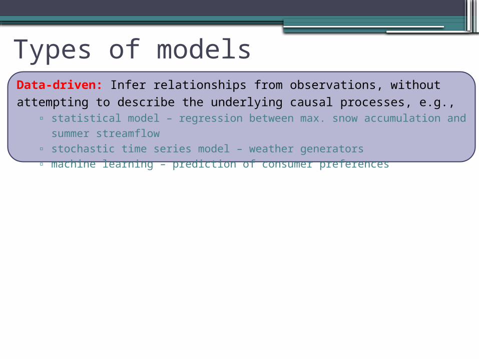
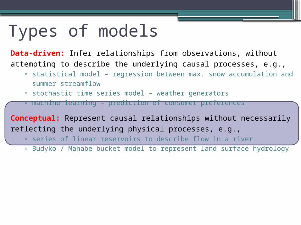
Types of modelsData-driven: Infer relationships from observations, without attempting to describe the underlying causal processes, e.g.,
▫ statistical model – regression between max. snow accumulation and summer streamflow
▫ stochastic time series model – weather generators▫ machine learning – prediction of consumer preferences
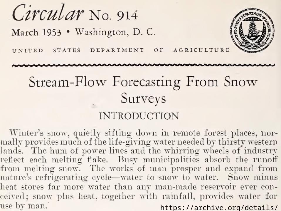
https://archive.org/details/streamflowforeca914work
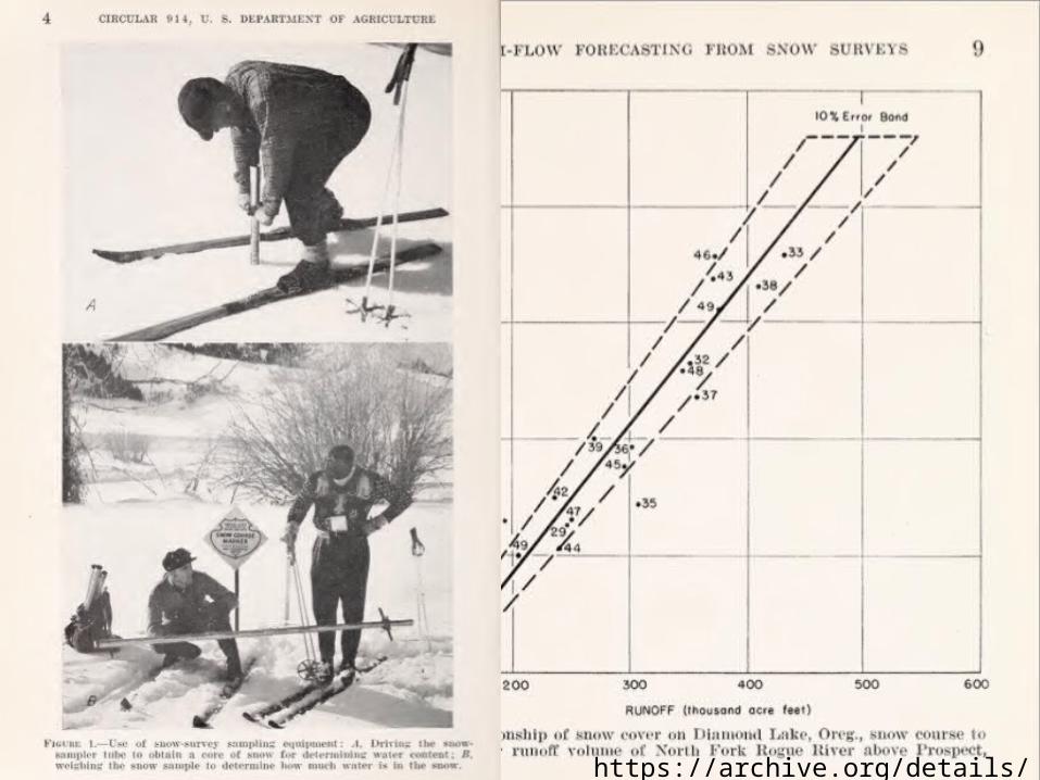
https://archive.org/details/streamflowforeca914work
Types of modelsData-driven: Infer relationships from observations, without attempting to describe the underlying causal processes, e.g.,
▫ statistical model – regression between max. snow accumulation and summer streamflow
▫ stochastic time series model – weather generators▫ machine learning – prediction of consumer preferences
Conceptual: Represent causal relationships without necessarily reflecting the underlying physical processes, e.g.,
▫ series of linear reservoirs to describe flow in a river▫ Budyko / Manabe bucket model to represent land surface hydrology
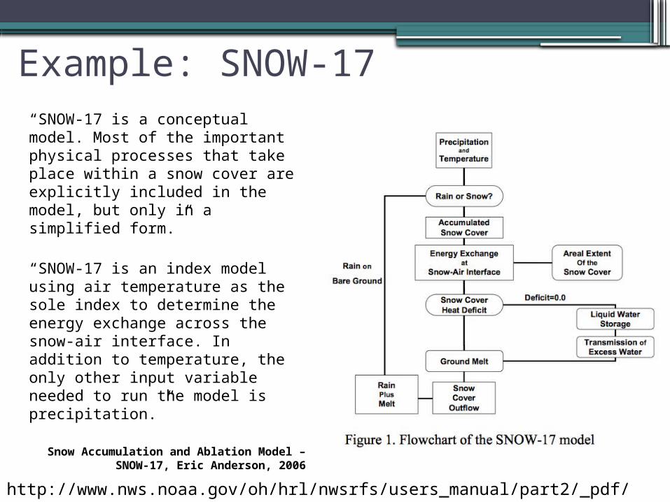
Example: SNOW-17“SNOW-17 is a conceptual model. Most of the important physical processes that take place within a snow cover are explicitly included in the model, but only in a simplified form.”
“SNOW-17 is an index model using air temperature as the sole index to determine the energy exchange across the snow-air interface. In addition to temperature, the only other input variable needed to run the model is precipitation.”
Snow Accumulation and Ablation Model – SNOW-17, Eric Anderson,
2006http://www.nws.noaa.gov/oh/hrl/nwsrfs/users_manual/part2/_pdf/22snow17.pdf
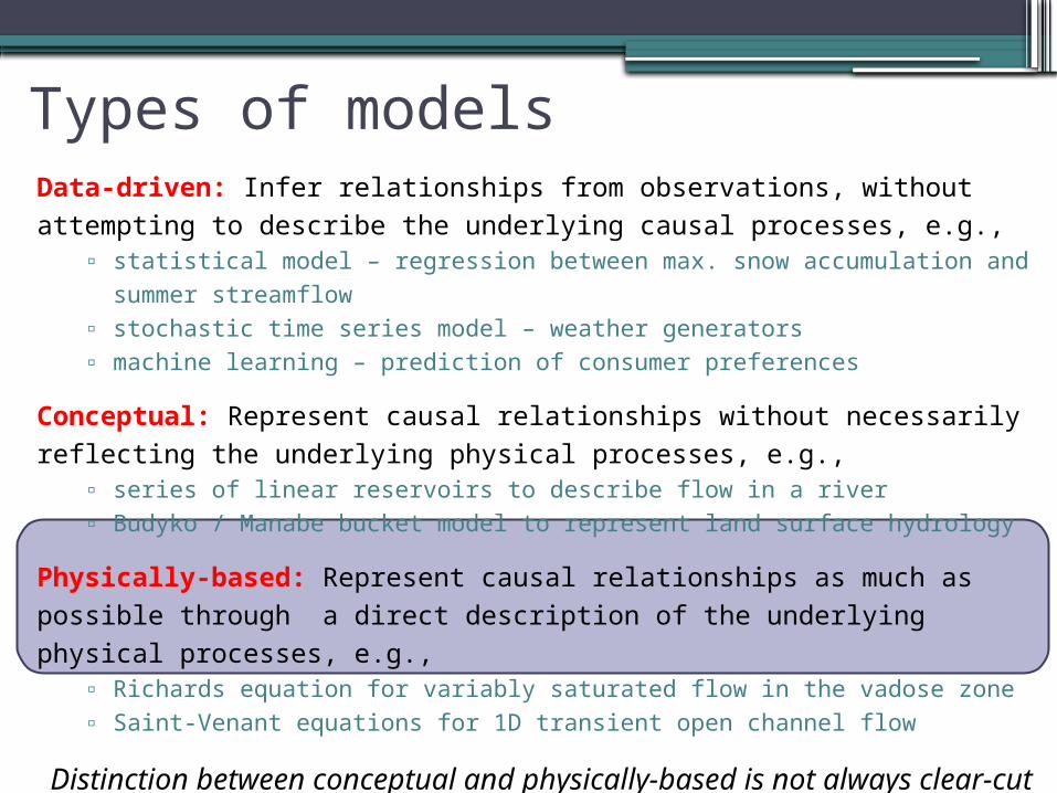
Types of modelsData-driven: Infer relationships from observations, without attempting to describe the underlying causal processes, e.g.,
▫ statistical model – regression between max. snow accumulation and summer streamflow
▫ stochastic time series model – weather generators▫ machine learning – prediction of consumer preferences
Conceptual: Represent causal relationships without necessarily reflecting the underlying physical processes, e.g.,
▫ series of linear reservoirs to describe flow in a river▫ Budyko / Manabe bucket model to represent land surface hydrology
Physically-based: Represent causal relationships as much as possible through a direct description of the underlying physical processes, e.g.,
▫ Richards equation for variably saturated flow in the vadose zone▫ Saint-Venant equations for 1D transient open channel flow
Distinction between conceptual and physically-based is not always clear-cut and often a function of scale (time, space)
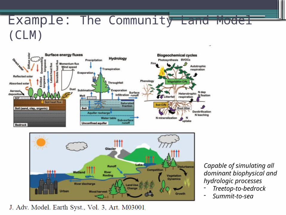
Example: The Community Land Model (CLM)
Capable of simulating all dominant biophysical and hydrologic processes- Treetop-to-bedrock- Summit-to-sea
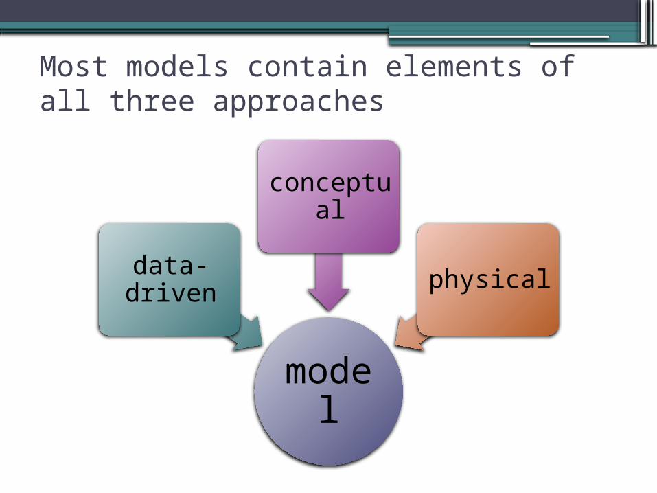
Most models contain elements of all three approaches
model
data-driven
conceptual
physical
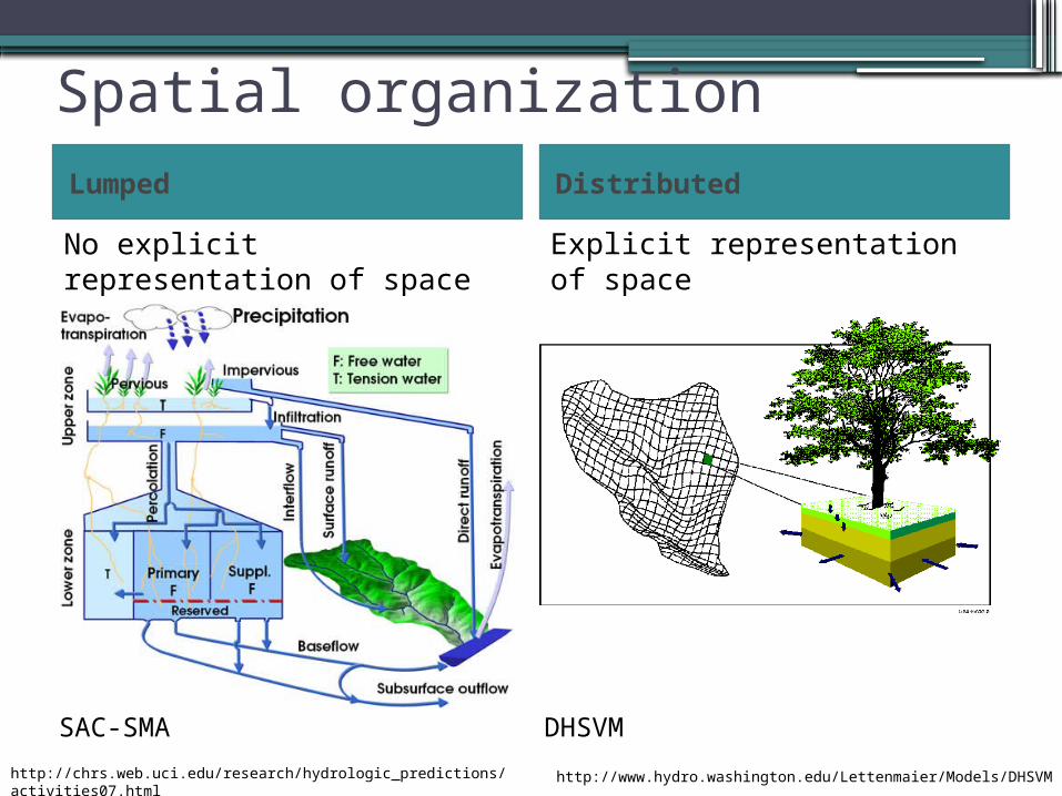
Spatial organizationLumped
No explicit representation of space
Distributed
Explicit representation of space
http://chrs.web.uci.edu/research/hydrologic_predictions/activities07.html
SAC-SMA DHSVM
http://www.hydro.washington.edu/Lettenmaier/Models/DHSVM
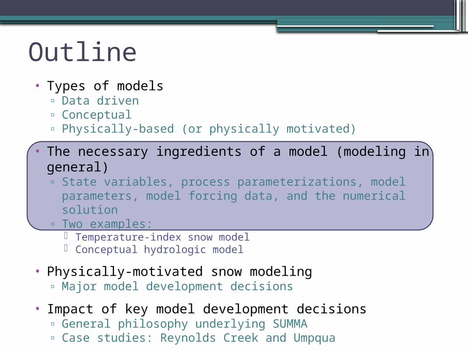
Outline• Types of models
▫ Data driven▫ Conceptual▫ Physically-based (or physically motivated)
• The necessary ingredients of a model (modeling in general)▫ State variables, process parameterizations, model parameters,
model forcing data, and the numerical solution▫ Two examples:
Temperature-index snow model Conceptual hydrologic model
• Physically-motivated snow modeling▫ Major model development decisions
• Impact of key model development decisions▫ General philosophy underlying SUMMA▫ Case studies: Reynolds Creek and Umpqua
• Summary and research needs
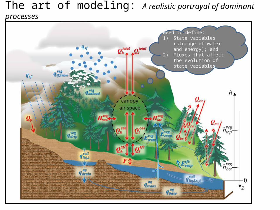
The art of modeling: A realistic portrayal of dominant processes
Need to define:1) State variables (storage of
water and energy); and2) Fluxes that affect the
evolution of state variables
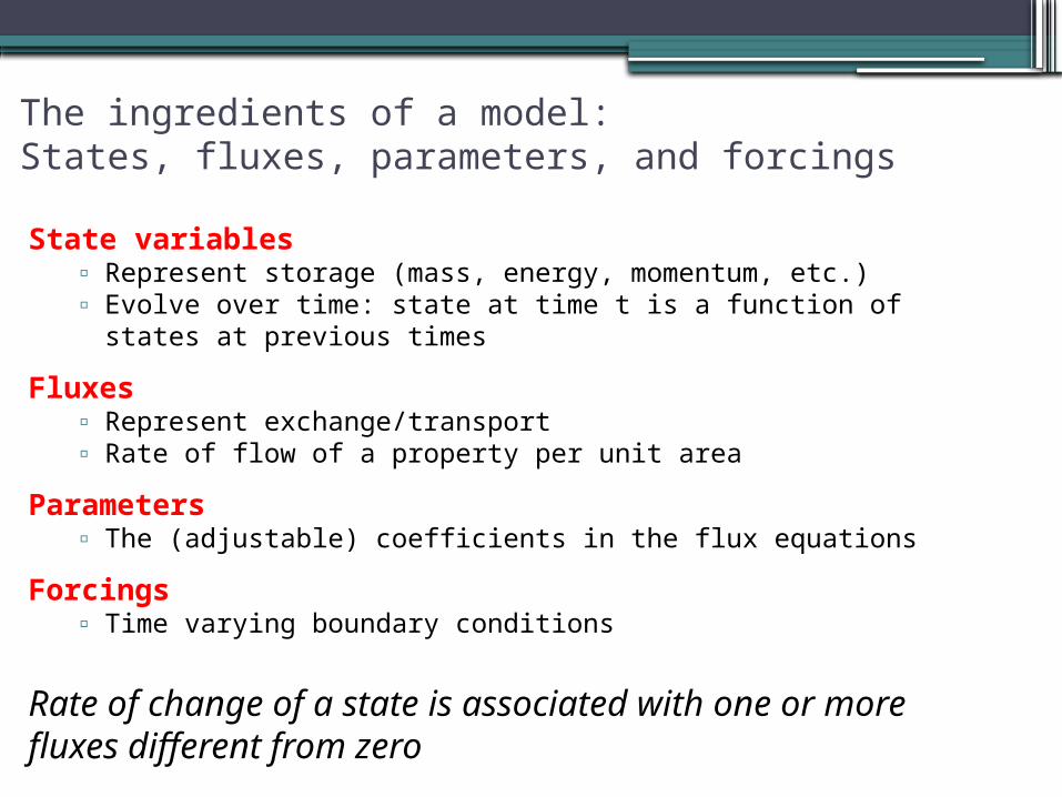
The ingredients of a model:States, fluxes, parameters, and forcings
State variables▫ Represent storage (mass, energy, momentum, etc.)▫ Evolve over time: state at time t is a function of states at
previous times
Fluxes▫ Represent exchange/transport▫ Rate of flow of a property per unit area
Parameters▫ The (adjustable) coefficients in the flux equations
Forcings▫ Time varying boundary conditions
Rate of change of a state is associated with one or more fluxes different from zero
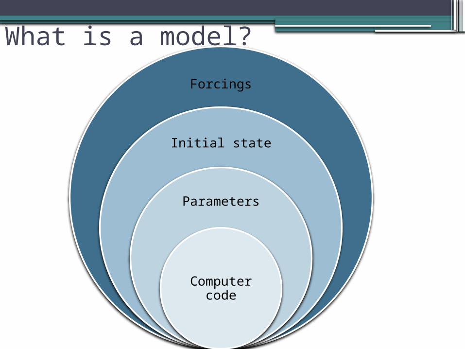
Forcings
Initial state
Parameters
Computer code
What is a model?
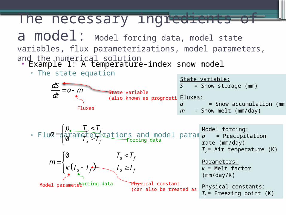
The necessary ingredients of a model: Model forcing data, model state variables, flux parameterizations, model parameters, and the numerical solution• Example 1: A temperature-index snow model
▫ The state equation
▫ Flux parameterizations and model parameters
▫ Numerical solution Simple in this case, since fluxes do not depend on state variables
dSa m
dt State variable
(also known as prognostic variable)
Fluxes
State variable:S = Snow storage (mm)
Fluxes:a = Snow accumulation (mm/day)m = Snow melt (mm/day)
0a f
a f
p T Ta
T T
0 a f
a f a f
T Tm
T T T T
Forcing data
Forcing dataModel parameter Physical constant(can also be treated as a model parameter)
Model forcing:p = Precipitation rate (mm/day)Ta = Air temperature (K)
Parameters:κ = Melt factor (mm/day/K)
Physical constants:Tf = Freezing point (K)
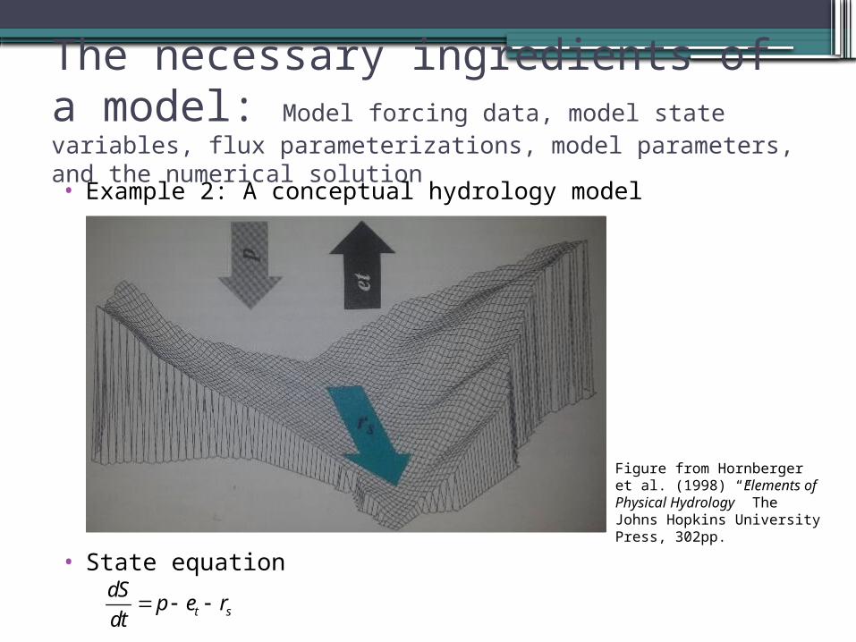
The necessary ingredients of a model: Model forcing data, model state variables, flux parameterizations, model parameters, and the numerical solution• Example 2: A conceptual hydrology model
• State equation
Figure from Hornberger et al. (1998) “Elements of Physical Hydrology” The Johns Hopkins University Press, 302pp.
t s
dSp e r
dt
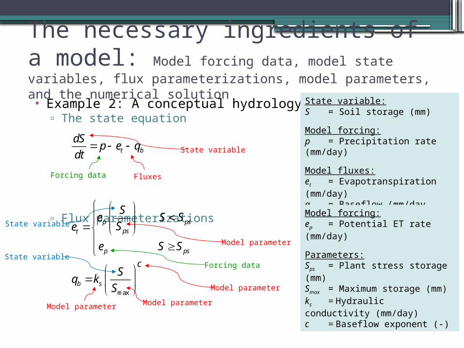
The necessary ingredients of a model: Model forcing data, model state variables, flux parameterizations, model parameters, and the numerical solution• Example 2: A conceptual hydrology model
▫ The state equation
▫ Flux parameterizations
▫ Numerical solution Care must be taken: model fluxes depend on state variables (numerical
daemons)
t b
dSp e q
dt State variable
Fluxes
State variable:S = Soil storage (mm)
Model forcing:p = Precipitation rate (mm/day)
Model fluxes:et = Evapotranspiration (mm/day)qb = Baseflow (mm/day
p pspst
p ps
Se S S
Se
e S S
maxb s
cS
q kS
Forcing data
Forcing data
Model forcing:ep = Potential ET rate (mm/day)
Parameters:Sps= Plant stress storage (mm)Smax = Maximum storage (mm)ks = Hydraulic conductivity (mm/day)c = Baseflow exponent (-)
Model parameter
Model parameter Model parameter
Model parameter
State variable
State variable
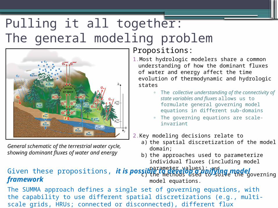
Pulling it all together:The general modeling problem
Propositions:1.Most hydrologic modelers share a common
understanding of how the dominant fluxes of water and energy affect the time evolution of thermodynamic and hydrologic states
▫ The collective understanding of the connectivity of state variables and fluxes allows us to formulate general governing model equations in different sub-domains
▫ The governing equations are scale-invariant
2.Key modeling decisions relate toa) the spatial discretization of the model domain;b) the approaches used to parameterize
individual fluxes (including model parameter values); and
c) the methods used to solve the governing model equations.
General schematic of the terrestrial water cycle, showing dominant fluxes of water and energy
Given these propositions, it is possible to develop a unifying model framework
The SUMMA approach defines a single set of governing equations, with the capability to use different spatial discretizations (e.g., multi-scale grids, HRUs; connected or disconnected), different flux parameterizations and model parameters, and different time stepping schemes
Outline• Types of models
▫ Data driven▫ Conceptual▫ Physically-based (or physically motivated)
• The necessary ingredients of a model (modeling in general)▫ State variables, process parameterizations, model parameters,
model forcing data, and the numerical solution▫ Two examples:
Temperature-index snow model Conceptual hydrologic model
• Physically-motivated snow modeling▫ Major model development decisions
• Impact of key model development decisions▫ General philosophy underlying SUMMA▫ Case studies: Reynolds Creek and Umpqua
• Summary and research needs
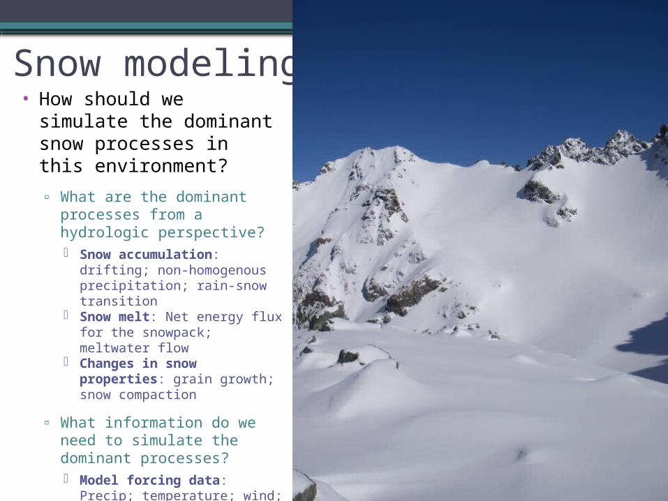
Snow modeling• How should we simulate
the dominant snow processes in this environment?
▫ What are the dominant processes from a hydrologic perspective? Snow accumulation:
drifting; non-homogenous precipitation; rain-snow transition
Snow melt: Net energy flux for the snowpack; meltwater flow
Changes in snow properties: grain growth; snow compaction
▫ What information do we need to simulate the dominant processes? Model forcing data: Precip;
temperature; wind; humidity; sw and lw radiation; (air pressure)
Model parameters: Drifting; snow albedo; turbulent heat fluxes; storage and transmission of liquid water in the snowpack
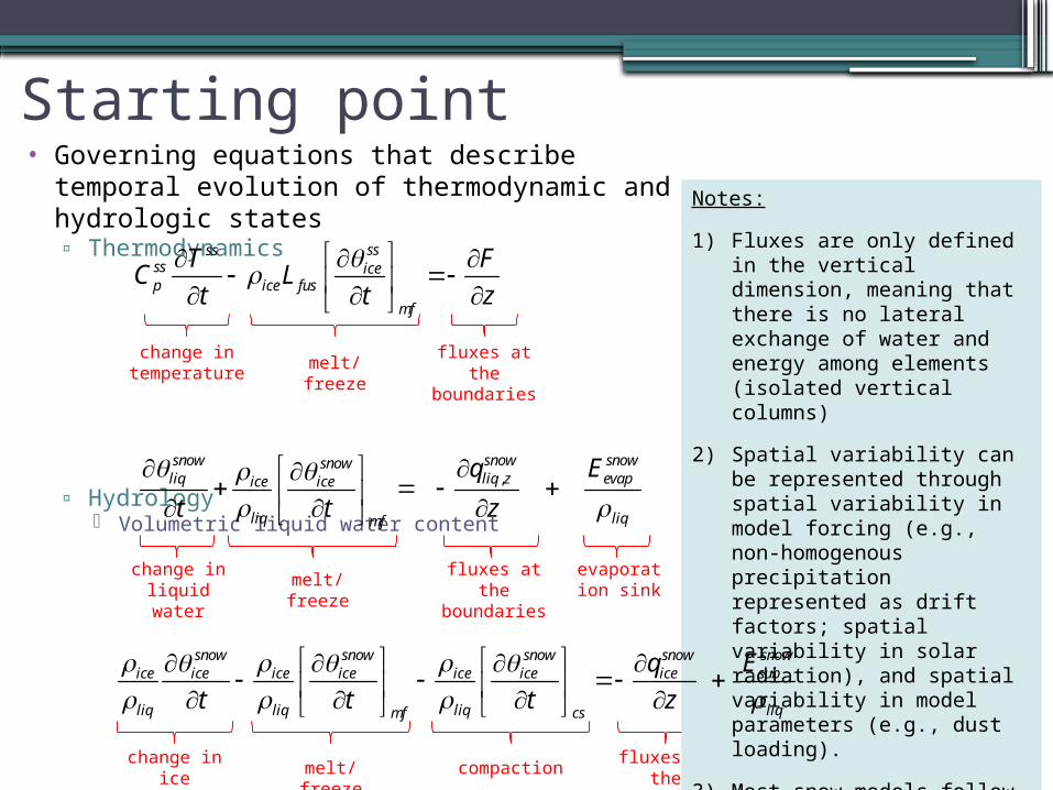
Starting point• Governing equations that describe temporal
evolution of thermodynamic and hydrologic states▫ Thermodynamics
▫ Hydrology Volumetric liquid water content
Volumetric ice content
ssssss icep ice fus
mf
T FC L
t t z
change in temperature
melt/freezefluxes at the boundaries
,snow snow snowsnowliq liq z evapice ice
liq liqmf
q E
t t z
change in liquid water
melt/freezefluxes at the boundaries
evaporation sink
snow snow snow snow snowice ice ice ice ice ice ice sub
liq liq liq liqmf cs
q E
t t t z
change in ice content
melt/freeze compactionfluxes at the boundaries
sublimation sink
Notes:
1) Fluxes are only defined in the vertical dimension, meaning that there is no lateral exchange of water and energy among elements (isolated vertical columns)
2) Spatial variability can be represented through spatial variability in model forcing (e.g., non-homogenous precipitation represented as drift factors; spatial variability in solar radiation), and spatial variability in model parameters (e.g., dust loading).
3) Most snow models follow these governing equations
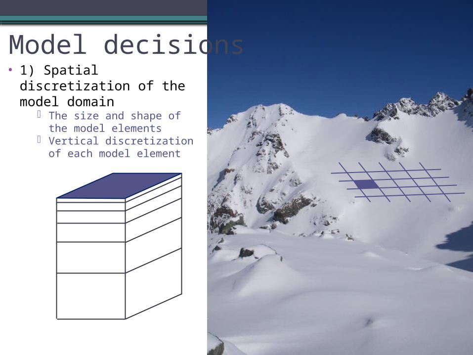
Model decisions• 1) Spatial discretization of
the model domain The size and shape of the
model elements Vertical discretization of
each model element
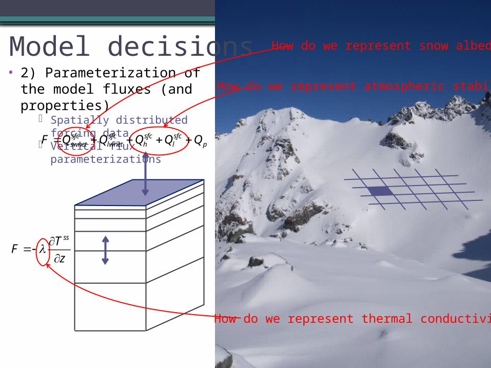
Model decisions• 2) Parameterization of the
model fluxes (and properties)
Spatially distributed forcing data
Vertical flux parameterizations
sfc sfc sfc sfcswnet lwnet h l pF Q Q Q Q Q
ssTF
z
How do we represent snow albedo?
How do we represent atmospheric stability?
How do we represent thermal conductivity?
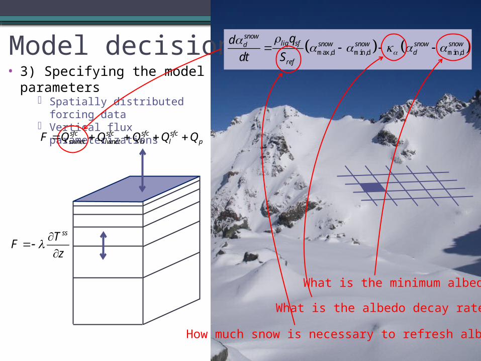
Model decisions• 3) Specifying the model
parameters Spatially distributed forcing
data Vertical flux
parameterizationssfc sfc sfc sfcswnet lwnet h l pF Q Q Q Q Q
ssTF
z
max,d min,d min,d
snowliq sf snow snow snow snowd
dref
qd
dt S
How much snow is necessary to refresh albedo?
What is the albedo decay rate?
What is the minimum albedo?
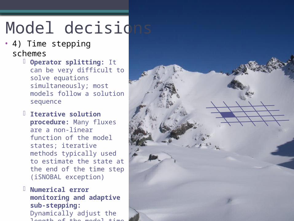
Model decisions• 4) Time stepping schemes
Operator splitting: It can be very difficult to solve equations simultaneously; most models follow a solution sequence
Iterative solution procedure: Many fluxes are a non-linear function of the model states; iterative methods typically used to estimate the state at the end of the time step (iSNOBAL exception)
Numerical error monitoring and adaptive sub-stepping: Dynamically adjust the length of the model time step to improve efficiency and reduce temporal truncation errors
Outline• Types of models
▫ Data driven▫ Conceptual▫ Physically-based (or physically motivated)
• The necessary ingredients of a model (modeling in general)▫ State variables, process parameterizations, model parameters,
model forcing data, and the numerical solution▫ Two examples:
Temperature-index snow model Conceptual hydrologic model
• Physically-motivated snow modeling▫ Major model development decisions
• Impact of key model development decisions▫ General philosophy underlying SUMMA▫ Case studies: Reynolds Creek and Umpqua
• Summary and research needs

Motivation
• Develop a Unified approach to modeling to understand model weaknesses and accelerate model development
• Address limitations of current modeling approaches▫ Poor understanding of differences among models
Model inter-comparison experiments flawed because too many differences among participating models to meaningfully attribute differences in model behavior to differences in model equations
▫ Poor understanding of model limitations Most models not constructed to enable a controlled and systematic
approach to model development and improvement
▫ Disparate (disciplinary) modeling efforts Poor representation of biophysical processes in hydrologic models Community cannot effectively work together, learn from each other,
and accelerate model development
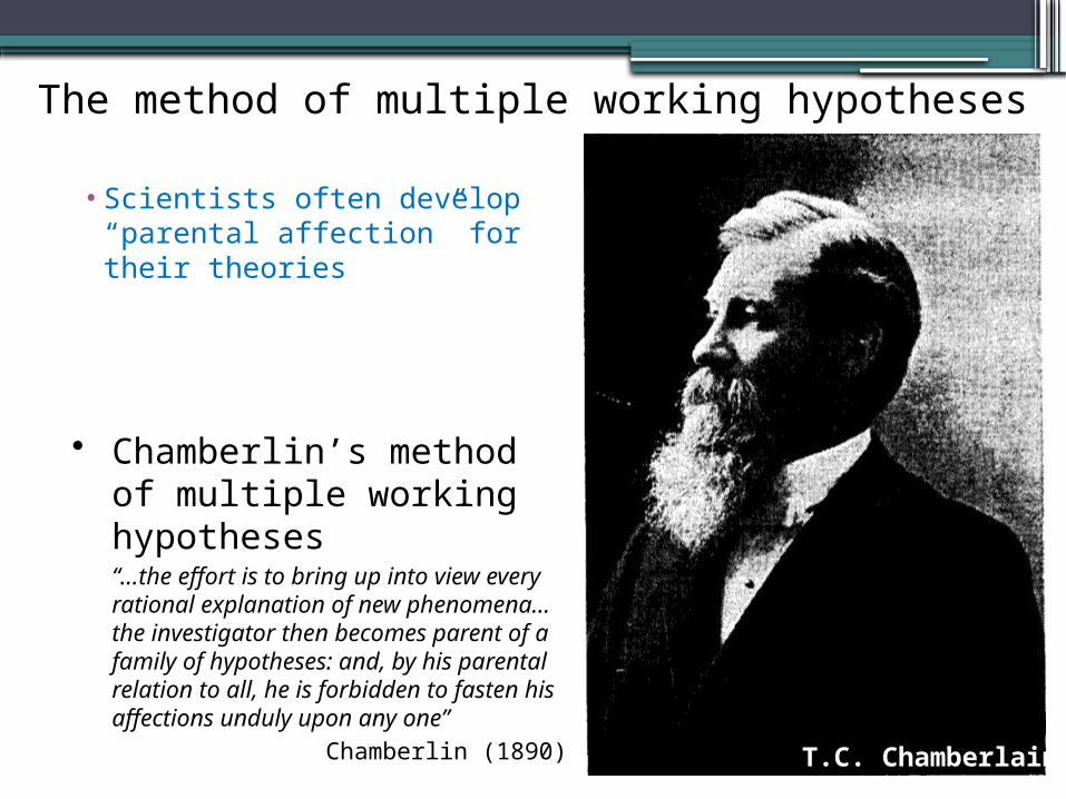
The method of multiple working hypotheses
• Scientists often develop “parental affection” for their theories
T.C. Chamberlain
• Chamberlin’s method of multiple working hypotheses
• “…the effort is to bring up into view every rational explanation of new phenomena… the investigator then becomes parent of a family of hypotheses: and, by his parental relation to all, he is forbidden to fasten his affections unduly upon any one”
• Chamberlin (1890)
Objectives• Advance capabilities in hydrologic prediction through a
unified approach to hydrological modeling▫ Improve model fidelity▫ Better characterize model uncertainty
33
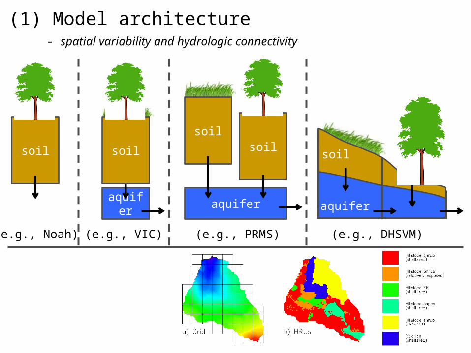
(1) Model architecture
soil soil
aquifer
(e.g., Noah) (e.g., VIC)
aquifer
soilsoil
(e.g., PRMS) (e.g., DHSVM)
aquifer
soil
- spatial variability and hydrologic connectivity
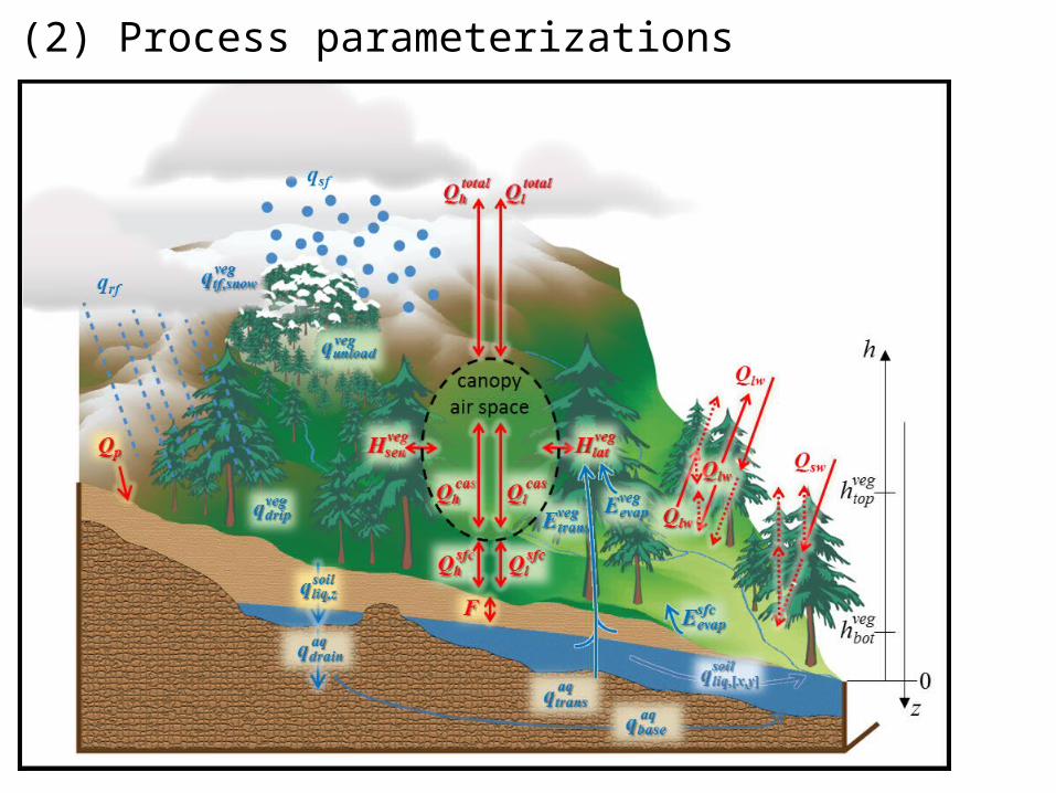
(2) Process parameterizations
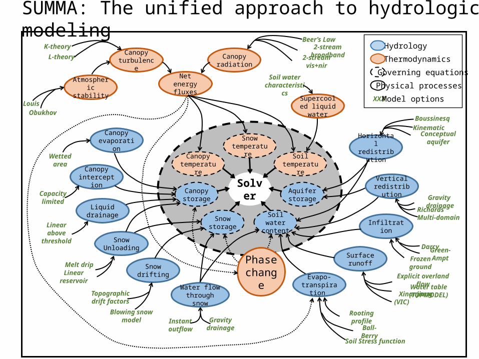
SUMMA: The unified approach to hydrologic modeling
Governing equations
Hydrology
Thermodynamics
Physical processes
XXX Model options
Evapo-transpiration
Infiltration
Surface runoff
SolverCanopy storage
Aquifer storage
Snow temperature
Snow Unloading
Canopy interception
Canopy evaporation
Water table (TOPMODEL)Xinanjiang (VIC)
Rooting profile
Green-AmptDarcy
Frozen ground
Richards’Gravity drainage
Multi-domain
Boussinesq
Conceptual aquifer
Instant outflow
Gravity drainage
Capacity limited
Wetted area
Soil water characteristics
Explicit overland flow
Atmospheric stability
Canopy radiation
Net energy fluxes
Beer’s Law
2-stream vis+nir
2-stream broadband
Kinematic
Liquid drainage
Linear above threshold
Soil Stress function Ball-Berry
Snow drifting
LouisObukhov
Melt drip
Linear reservoir
Topographic drift factors
Blowing snowmodel
Snowstorage
Soil water content
Canopy temperature
Soil temperature
Phase change
Horizontal redistribution
Water flow through snow
Canopy turbulence
Supercooled liquid water
K-theory
L-theory
Vertical redistribution
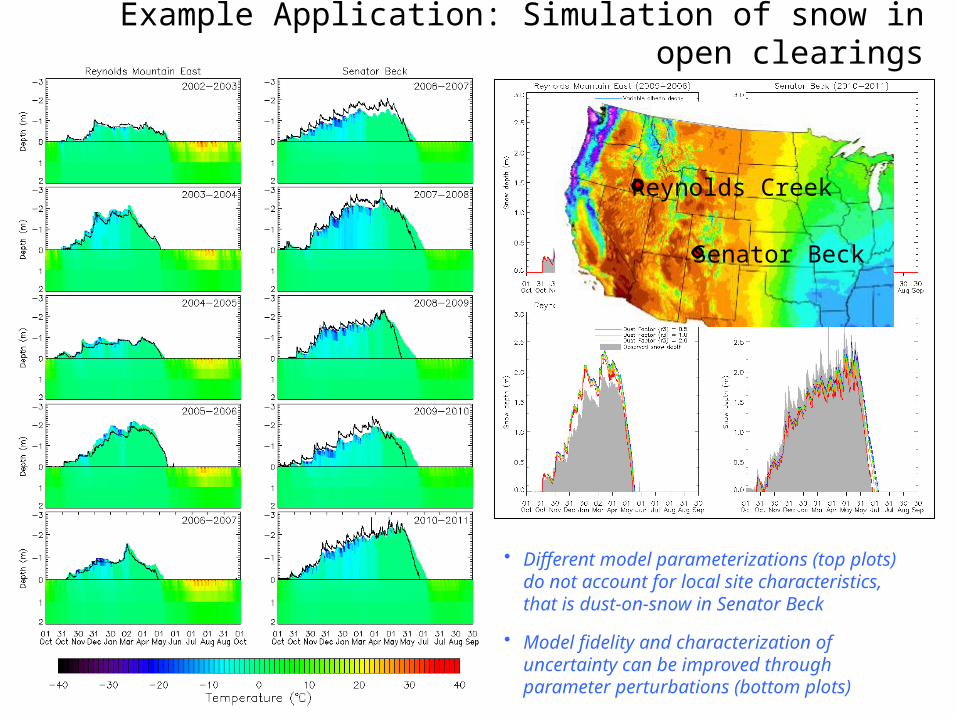
Example Application: Simulation of snow in open clearings
• Different model parameterizations (top plots) do not account for local site characteristics, that is dust-on-snow in Senator Beck
• Model fidelity and characterization of uncertainty can be improved through parameter perturbations (bottom plots)
Reynolds Creek
Senator Beck
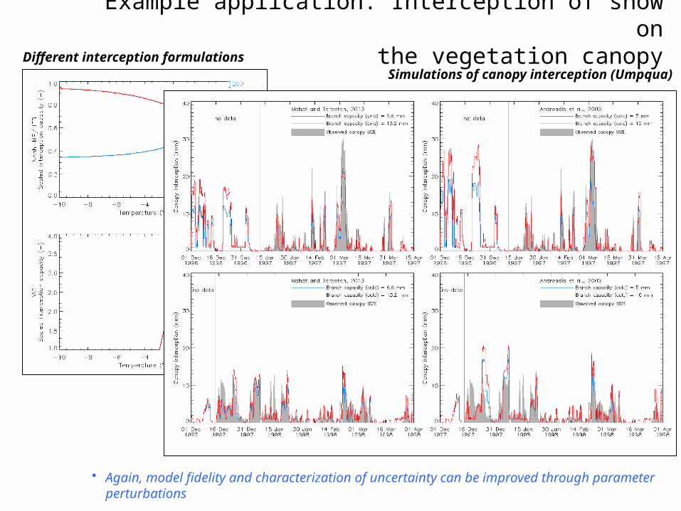
Example application: Interception of snow onthe vegetation canopy
• Again, model fidelity and characterization of uncertainty can be improved through parameter perturbations
Different interception formulationsSimulations of canopy interception (Umpqua)
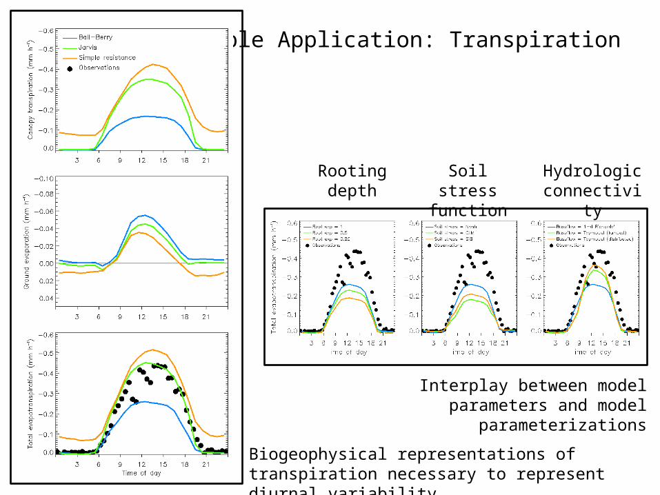
Example Application: Transpiration
Biogeophysical representations of transpiration necessary to represent diurnal variability
Interplay between model parameters and model parameterizations
Rooting depth
Hydrologic connectivity
Soil stress function
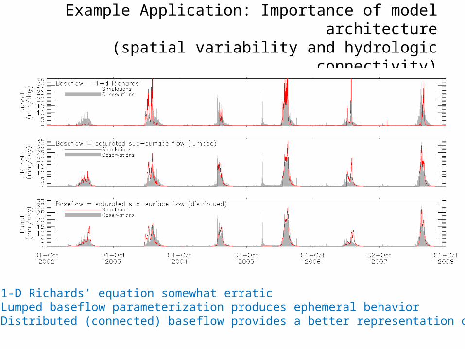
Example Application: Importance of model architecture
(spatial variability and hydrologic connectivity)
1-D Richards’ equation somewhat erratic Lumped baseflow parameterization produces ephemeral behavior Distributed (connected) baseflow provides a better representation of runoff
Outline• Types of models
▫ Data driven▫ Conceptual▫ Physically-based (or physically motivated)
• The necessary ingredients of a model (modeling in general)▫ State variables, process parameterizations, model parameters,
model forcing data, and the numerical solution▫ Two examples:
Temperature-index snow model Conceptual hydrologic model
• Physically-motivated snow modeling▫ Major model development decisions
• Impact of key model development decisions▫ General philosophy underlying SUMMA▫ Case studies: Reynolds Creek and Umpqua
• Summary and research needs
Summary
• Objectives▫ Better representation of observed processes (model fidelity)▫ More precise representation of model uncertainty
• Approach: Detailed evaluation of competing modeling approaches▫ Recognize that different models based on the same set of governing
equations▫ Defines a “master modeling template” to reconstruct existing
modeling approaches and derive new modeling methodologies▫ Provides a systematic and controlled approach to model and
evaluation
• Outcomes▫ Provided guidance for future model development▫ Improved understanding of the impact of different types of model
development decisions▫ Improved operational applicability of process-based models
Summary and research needs
• Model fidelity▫ Comprehensive review/analysis of different modelling approaches
has helped identify a preferable set of modeling methods Some obvious: biophysical representation of transpiration, two-stream canopy
radiation, dust deposition on snow, etc.▫ Need to place much more emphasis on parameter estimation
A science problem rather than a curve-fitting exercise Focus on relating geophysical attributes to model parameters Use multiple datasets at different scales to reduce compensatory errors
• Model uncertainty▫ Improved understanding of suitable methods to characterize
uncertainty in different parts of the model Distinguish between decisions on process representation versus decisions on choice
of constitutive functions▫ Recognize shortcomings of using multi-physics and multi-model
approaches to characterize uncertainty Competing models can provide the wrong results for the same reasons (albedo
example)▫ Need to approach uncertainty quantification from a physical
perspective Inverse methods are plagued by compensatory interactions among different sources
of uncertainty… difficult to infer meaningful uncertainty estimates Progress possible through a more refined analysis of individual model development
decisions
Exercises with a toy model
Martyn Clark (NCAR/RAL)Dmitri Kavetski (University of Adelaide, Australia)
PRMS SACRAMENTO
ARNO/VICTOPMODELwlt fld sat
lzZ
uzZ
pe
S1T S1
F
S2T
S2FA
S2F
B
qif
qbA
qbB
q12
wlt fld sat
lzZ
uzZ
e p
qsx
qb
q12
S2
S1
wlt fld sat
GFLWR lzZ
uzZ
S2
S1
e p
q12
qsx
qb
e p
wlt sat
S1TA
fld
lzZ
uzZqsx
qif
qb
S1TB S1
F
q12
S2
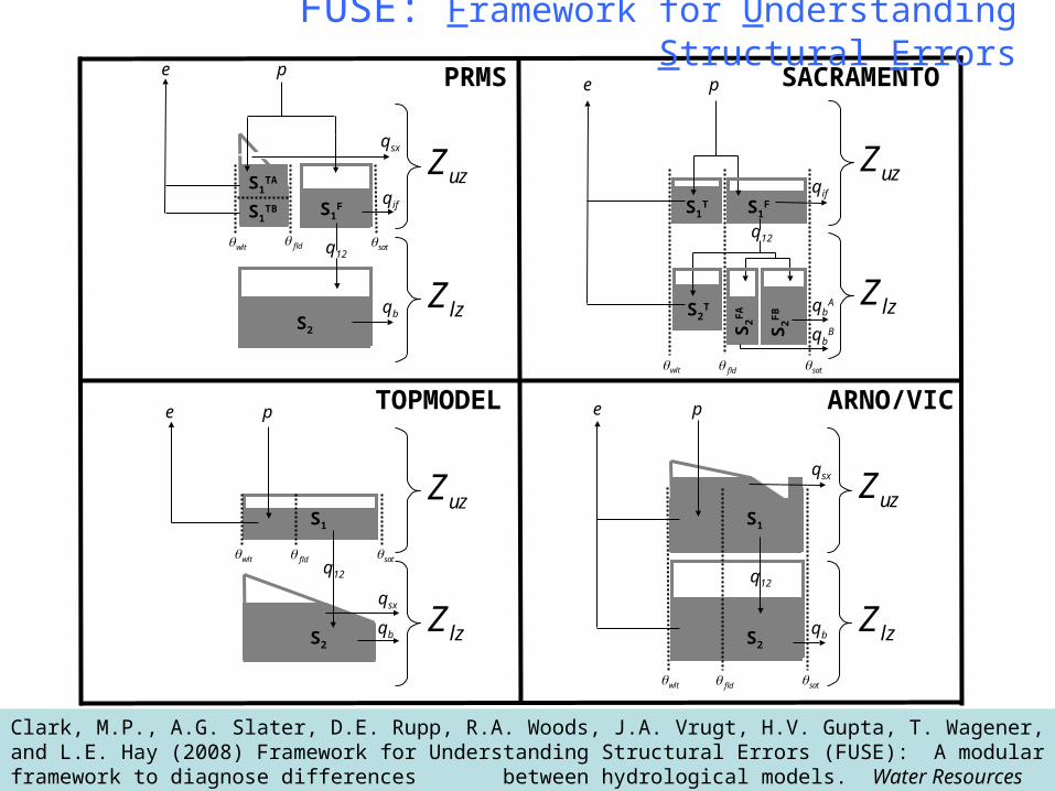
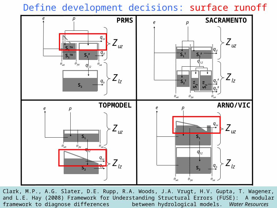
Clark, M.P., A.G. Slater, D.E. Rupp, R.A. Woods, J.A. Vrugt, H.V. Gupta, T. Wagener, and L.E. Hay (2008) Framework for Understanding Structural Errors (FUSE): A modular framework to diagnose differences between hydrological models. Water Resources Research, 44, W00B02, doi:10.1029/2007WR006735.
FUSE: Framework for Understanding Structural Errors
PRMS SACRAMENTO
ARNO/VICTOPMODELwlt fld sat
lzZ
uzZ
pe
S1T S1
F
S2T
S2FA
S2F
B
qif
qbA
qbB
q12
wlt fld sat
lzZ
uzZ
e p
qsx
qb
q12
S2
S1
wlt fld sat
GFLWR lzZ
uzZ
S2
S1
e p
q12
qsx
qb
e p
wlt sat
S1TA
fld
lzZ
uzZqsx
qif
qb
S1TB S1
F
q12
S2
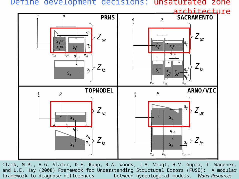
Clark, M.P., A.G. Slater, D.E. Rupp, R.A. Woods, J.A. Vrugt, H.V. Gupta, T. Wagener, and L.E. Hay (2008) Framework for Understanding Structural Errors (FUSE): A modular framework to diagnose differences between hydrological models. Water Resources Research, 44, W00B02, doi:10.1029/2007WR006735.
Define development decisions: unsaturated zone architecture
PRMS SACRAMENTO
ARNO/VICTOPMODELwlt fld sat
lzZ
uzZ
pe
S1T S1
F
S2T
S2FA
S2F
B
qif
qbA
qbB
q12
wlt fld sat
lzZ
uzZ
e p
qsx
qb
q12
S2
S1
wlt fld sat
GFLWR lzZ
uzZ
S2
S1
e p
q12
qsx
qb
e p
wlt sat
S1TA
fld
lzZ
uzZqsx
qif
qb
S1TB S1
F
q12
S2
Clark, M.P., A.G. Slater, D.E. Rupp, R.A. Woods, J.A. Vrugt, H.V. Gupta, T. Wagener, and L.E. Hay (2008) Framework for Understanding Structural Errors (FUSE): A modular framework to diagnose differences between hydrological models. Water Resources Research, 44, W00B02, doi:10.1029/2007WR006735.
Define development decisions: saturated zone / baseflow
PRMS SACRAMENTO
ARNO/VICTOPMODELwlt fld sat
lzZ
uzZ
pe
S1T S1
F
S2T
S2FA
S2F
B
qif
qbA
qbB
q12
wlt fld sat
lzZ
uzZ
e p
qsx
qb
q12
S2
S1
wlt fld sat
GFLWR lzZ
uzZ
S2
S1
e p
q12
qsx
qb
e p
wlt sat
S1TA
fld
lzZ
uzZqsx
qif
qb
S1TB S1
F
q12
S2
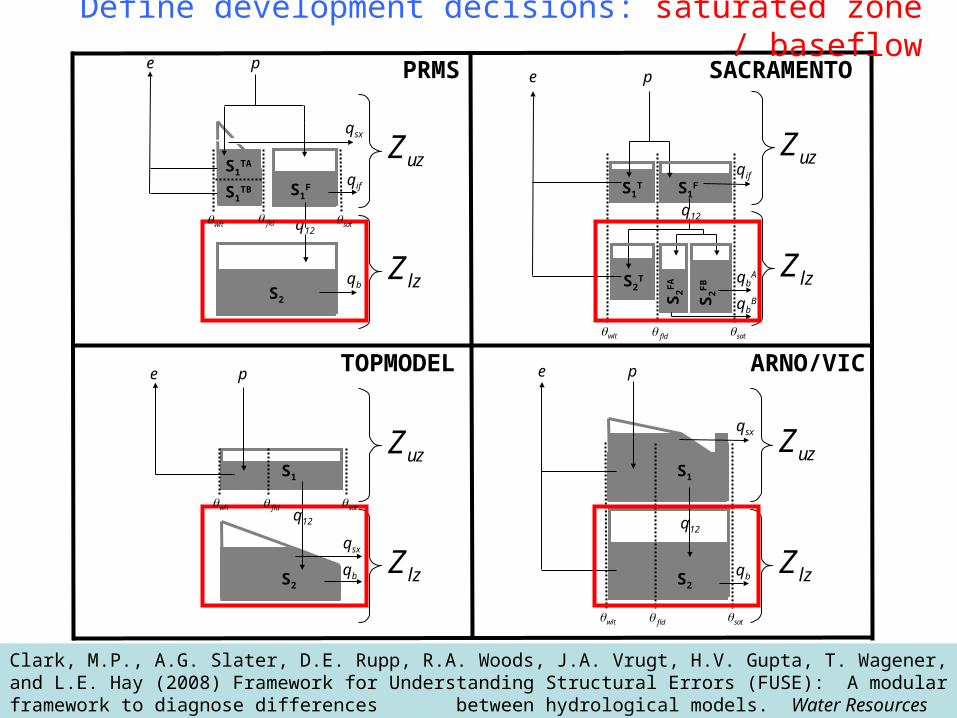
Clark, M.P., A.G. Slater, D.E. Rupp, R.A. Woods, J.A. Vrugt, H.V. Gupta, T. Wagener, and L.E. Hay (2008) Framework for Understanding Structural Errors (FUSE): A modular framework to diagnose differences between hydrological models. Water Resources Research, 44, W00B02, doi:10.1029/2007WR006735.
Define development decisions: vertical drainage
PRMS SACRAMENTO
ARNO/VICTOPMODELwlt fld sat
lzZ
uzZ
pe
S1T S1
F
S2T
S2FA
S2F
B
qif
qbA
qbB
q12
wlt fld sat
lzZ
uzZ
e p
qsx
qb
q12
S2
S1
wlt fld sat
GFLWR lzZ
uzZ
S2
S1
e p
q12
qsx
qb
e p
wlt sat
S1TA
fld
lzZ
uzZqsx
qif
qb
S1TB S1
F
q12
S2
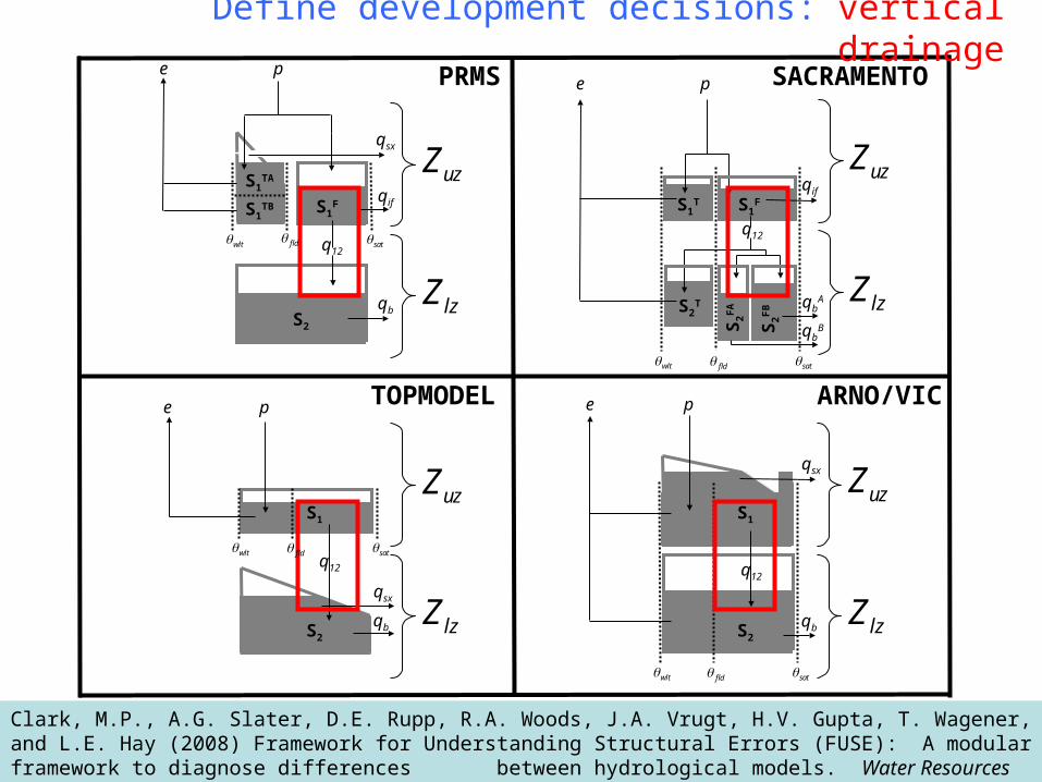
Clark, M.P., A.G. Slater, D.E. Rupp, R.A. Woods, J.A. Vrugt, H.V. Gupta, T. Wagener, and L.E. Hay (2008) Framework for Understanding Structural Errors (FUSE): A modular framework to diagnose differences between hydrological models. Water Resources Research, 44, W00B02, doi:10.1029/2007WR006735.
Define development decisions: surface runoff
PRMS SACRAMENTO
ARNO/VICTOPMODELwlt fld sat
lzZ
uzZ
pe
S1T S1
F
S2T
S2FA
S2F
B
qif
qbA
qbB
q12
wlt fld sat
lzZ
uzZ
e p
qsx
qb
q12
S2
S1
wlt fld sat
GFLWR lzZ
uzZ
S2
S1
e p
q12
qsx
qb
e p
wlt sat
S1TA
fld
lzZ
uzZqsx
qif
qb
S1TB S1
F
q12
S2
Clark, M.P., A.G. Slater, D.E. Rupp, R.A. Woods, J.A. Vrugt, H.V. Gupta, T. Wagener, and L.E. Hay (2008) Framework for Understanding Structural Errors (FUSE): A modular framework to diagnose differences between hydrological models. Water Resources Research, 44, W00B02, doi:10.1029/2007WR006735.
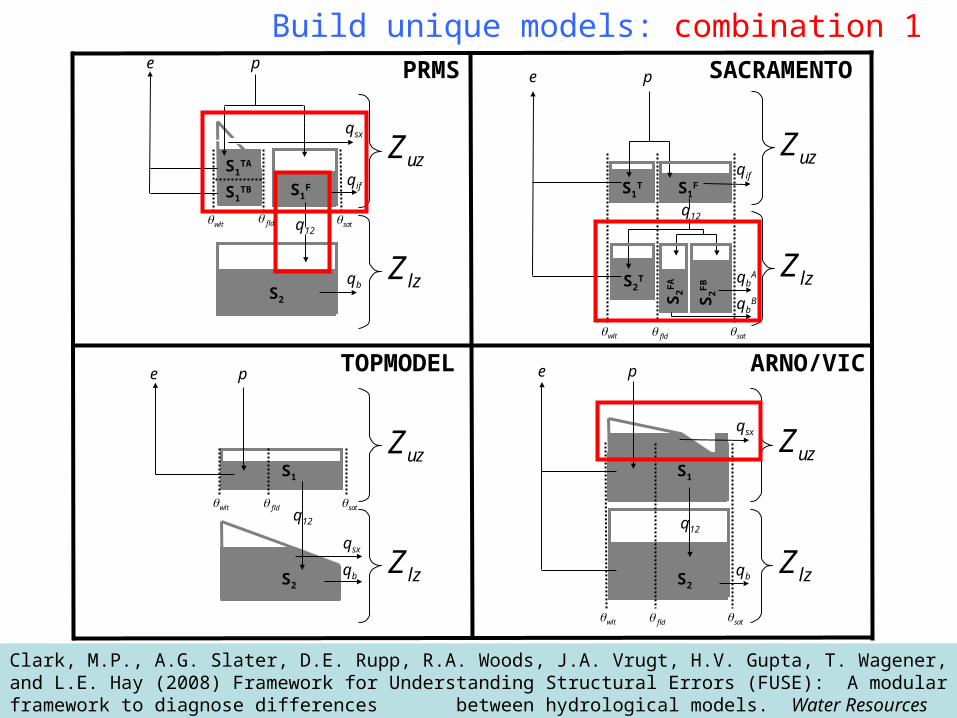
Build unique models: combination 1
PRMS SACRAMENTO
ARNO/VICTOPMODELwlt fld sat
lzZ
uzZ
pe
S1T S1
F
S2T
S2FA
S2F
B
qif
qbA
qbB
q12
wlt fld sat
lzZ
uzZ
e p
qsx
qb
q12
S2
S1
wlt fld sat
GFLWR lzZ
uzZ
S2
S1
e p
q12
qsx
qb
e p
wlt sat
S1TA
fld
lzZ
uzZqsx
qif
qb
S1TB S1
F
q12
S2
Clark, M.P., A.G. Slater, D.E. Rupp, R.A. Woods, J.A. Vrugt, H.V. Gupta, T. Wagener, and L.E. Hay (2008) Framework for Understanding Structural Errors (FUSE): A modular framework to diagnose differences between hydrological models. Water Resources Research, 44, W00B02, doi:10.1029/2007WR006735.
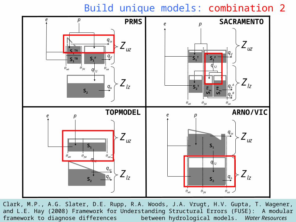
Build unique models: combination 2
PRMS SACRAMENTO
ARNO/VICTOPMODELwlt fld sat
lzZ
uzZ
pe
S1T S1
F
S2T
S2FA
S2F
B
qif
qbA
qbB
q12
wlt fld sat
lzZ
uzZ
e p
qsx
qb
q12
S2
S1
wlt fld sat
GFLWR lzZ
uzZ
S2
S1
e p
q12
qsx
qb
e p
wlt sat
S1TA
fld
lzZ
uzZqsx
qif
qb
S1TB S1
F
q12
S2
Clark, M.P., A.G. Slater, D.E. Rupp, R.A. Woods, J.A. Vrugt, H.V. Gupta, T. Wagener, and L.E. Hay (2008) Framework for Understanding Structural Errors (FUSE): A modular framework to diagnose differences between hydrological models. Water Resources Research, 44, W00B02, doi:10.1029/2007WR006735.
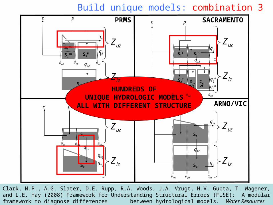
Build unique models: combination 3
HUNDREDS OFUNIQUE HYDROLOGIC MODELS
ALL WITH DIFFERENT STRUCTURE
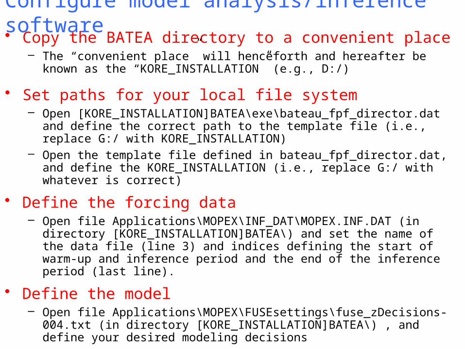
Configure model analysis/inference software• Copy the BATEA directory to a convenient place
– The “convenient place” will henceforth and hereafter be known as the “KORE_INSTALLATION” (e.g., D:/)
• Set paths for your local file system– Open [KORE_INSTALLATION]BATEA\exe\bateau_fpf_director.dat and define the
correct path to the template file (i.e., replace G:/ with KORE_INSTALLATION)– Open the template file defined in bateau_fpf_director.dat, and define the
KORE_INSTALLATION (i.e., replace G:/ with whatever is correct)
• Define the forcing data– Open file Applications\MOPEX\INF_DAT\MOPEX.INF.DAT (in directory
[KORE_INSTALLATION]BATEA\) and set the name of the data file (line 3) and indices defining the start of warm-up and inference period and the end of the inference period (last line).
• Define the model– Open file Applications\MOPEX\FUSEsettings\fuse_zDecisions-004.txt (in
directory [KORE_INSTALLATION]BATEA\) , and define your desired modeling decisions
• Start analysis/inference– Click on the appropriate executable in [KORE_INSTALLATION]BATEA\exe
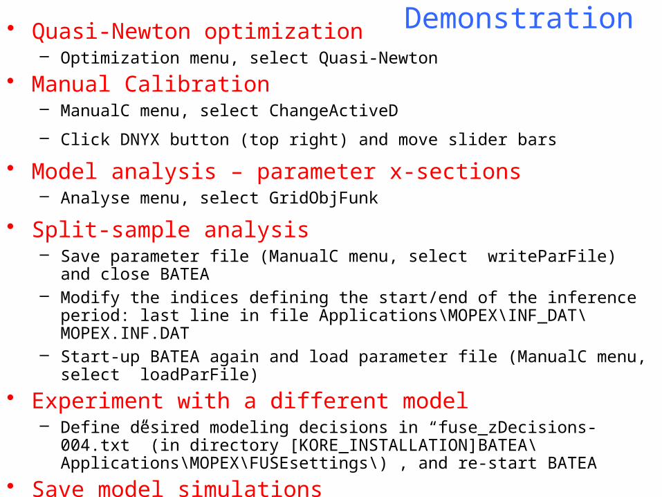
Demonstration• Quasi-Newton optimization– Optimization menu, select Quasi-Newton
• Manual Calibration– ManualC menu, select ChangeActiveD
– Click DNYX button (top right) and move slider bars
• Model analysis – parameter x-sections– Analyse menu, select GridObjFunk
• Split-sample analysis– Save parameter file (ManualC menu, select writeParFile) and close BATEA– Modify the indices defining the start/end of the inference period: last line in file
Applications\MOPEX\INF_DAT\MOPEX.INF.DAT– Start-up BATEA again and load parameter file (ManualC menu, select
loadParFile)
• Experiment with a different model– Define desired modeling decisions in “fuse_zDecisions-004.txt” (in directory
[KORE_INSTALLATION]BATEA\Applications\MOPEX\FUSEsettings\) , and re-start BATEA
• Save model simulations– ManualC menu, select writeAllDataFile
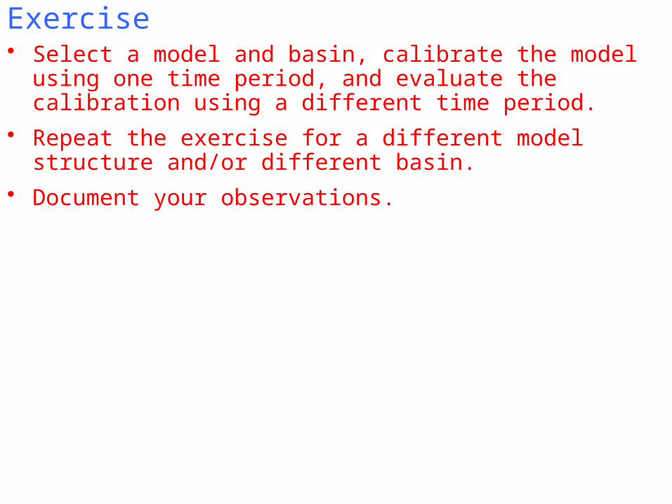
Exercise• Select a model and basin, calibrate the model using one time
period, and evaluate the calibration using a different time period.
• Repeat the exercise for a different model structure and/or different basin.
• Document your observations.
QUESTIONS ???