Embed Size (px)
Citation preview
December 2013 Prepared for: Maryland Transportation Authority Prepared by:
Maryland Transportation Authority I-95 Express Toll Lanes Comprehensive Traffic and Toll Revenue Study
I-95 ETL Comprehensive Traffic and Toll Revenue Study Maryland Transportation Authority
Page i
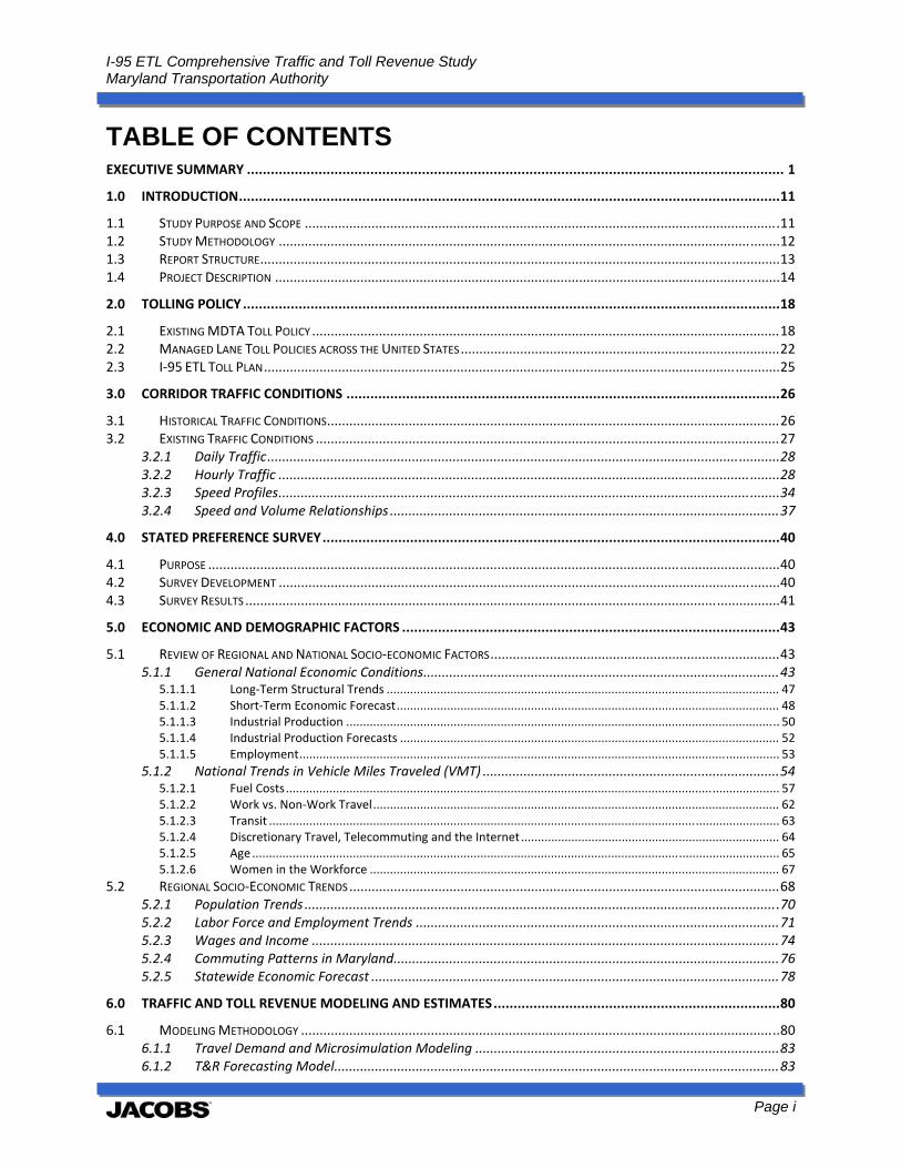
TABLE OF CONTENTS EXECUTIVE SUMMARY ....................................................................................................................................... 1
1.0 INTRODUCTION ........................................................................................................................................ 11
1.1 STUDY PURPOSE AND SCOPE ................................................................................................................................ 11 1.2 STUDY METHODOLOGY ....................................................................................................................................... 12 1.3 REPORT STRUCTURE ............................................................................................................................................ 13 1.4 PROJECT DESCRIPTION ........................................................................................................................................ 14
2.0 TOLLING POLICY ....................................................................................................................................... 18
2.1 EXISTING MDTA TOLL POLICY .............................................................................................................................. 18 2.2 MANAGED LANE TOLL POLICIES ACROSS THE UNITED STATES ...................................................................................... 22 2.3 I‐95 ETL TOLL PLAN ........................................................................................................................................... 25
3.0 CORRIDOR TRAFFIC CONDITIONS ............................................................................................................. 26
3.1 HISTORICAL TRAFFIC CONDITIONS .......................................................................................................................... 26 3.2 EXISTING TRAFFIC CONDITIONS ............................................................................................................................. 27
3.2.1 Daily Traffic .......................................................................................................................................... 28 3.2.2 Hourly Traffic ....................................................................................................................................... 28 3.2.3 Speed Profiles ....................................................................................................................................... 34 3.2.4 Speed and Volume Relationships ......................................................................................................... 37
4.0 STATED PREFERENCE SURVEY ................................................................................................................... 40
4.1 PURPOSE .......................................................................................................................................................... 40 4.2 SURVEY DEVELOPMENT ....................................................................................................................................... 40 4.3 SURVEY RESULTS ................................................................................................................................................ 41
5.0 ECONOMIC AND DEMOGRAPHIC FACTORS ............................................................................................... 43
5.1 REVIEW OF REGIONAL AND NATIONAL SOCIO‐ECONOMIC FACTORS .............................................................................. 43 5.1.1 General National Economic Conditions ................................................................................................ 43
5.1.1.1 Long‐Term Structural Trends ..................................................................................................................... 47 5.1.1.2 Short‐Term Economic Forecast .................................................................................................................. 48 5.1.1.3 Industrial Production ................................................................................................................................. 50 5.1.1.4 Industrial Production Forecasts ................................................................................................................. 52 5.1.1.5 Employment ............................................................................................................................................... 53
5.1.2 National Trends in Vehicle Miles Traveled (VMT) ................................................................................ 54 5.1.2.1 Fuel Costs ................................................................................................................................................... 57 5.1.2.2 Work vs. Non‐Work Travel ......................................................................................................................... 62 5.1.2.3 Transit ........................................................................................................................................................ 63 5.1.2.4 Discretionary Travel, Telecommuting and the Internet ............................................................................. 64 5.1.2.5 Age ............................................................................................................................................................. 65 5.1.2.6 Women in the Workforce .......................................................................................................................... 67
5.2 REGIONAL SOCIO‐ECONOMIC TRENDS .................................................................................................................... 68 5.2.1 Population Trends ................................................................................................................................ 70 5.2.2 Labor Force and Employment Trends .................................................................................................. 71 5.2.3 Wages and Income .............................................................................................................................. 74 5.2.4 Commuting Patterns in Maryland ........................................................................................................ 76 5.2.5 Statewide Economic Forecast .............................................................................................................. 78
6.0 TRAFFIC AND TOLL REVENUE MODELING AND ESTIMATES ........................................................................ 80
6.1 MODELING METHODOLOGY ................................................................................................................................. 80 6.1.1 Travel Demand and Microsimulation Modeling .................................................................................. 83 6.1.2 T&R Forecasting Model ........................................................................................................................ 83
I-95 ETL Comprehensive Traffic and Toll Revenue Study Maryland Transportation Authority
Page ii
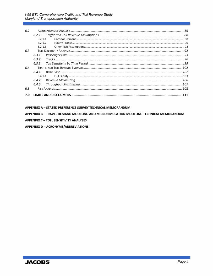
6.2 ASSUMPTIONS OF ANALYSIS ................................................................................................................................. 85 6.2.1 Traffic and Toll Revenue Assumptions ................................................................................................. 88
6.2.1.1 Corridor Demand ....................................................................................................................................... 88 6.2.1.2 Hourly Profile ............................................................................................................................................. 90 6.2.1.3 Other T&R Assumptions ............................................................................................................................. 92
6.3 TOLL SENSITIVITY ANALYSES ................................................................................................................................. 92 6.3.1 Passenger Cars ..................................................................................................................................... 93 6.3.2 Trucks ................................................................................................................................................... 96 6.3.3 Toll Sensitivity by Time Period .............................................................................................................. 99
6.4 TRAFFIC AND TOLL REVENUE ESTIMATES ............................................................................................................... 102 6.4.1 Base Case ........................................................................................................................................... 102
6.4.1.1 Full Facility ............................................................................................................................................... 103 6.4.2 Revenue Maximizing .......................................................................................................................... 106 6.4.3 Throughput Maximizing ..................................................................................................................... 107
6.5 RISK ANALYSIS ................................................................................................................................................. 108
7.0 LIMITS AND DISCLAIMERS ...................................................................................................................... 111
APPENDIX A – STATED PREFERENCE SURVEY TECHNICAL MEMORANDUM
APPENDIX B – TRAVEL DEMAND MODELING AND MICROSIMULATION MODELING TECHNICAL MEMORANDUM
APPENDIX C – TOLL SENSITIVITY ANALYSES
APPENDIX D – ACRONYMS/ABBREVIATIONS
I-95 ETL Comprehensive Traffic and Toll Revenue Study Maryland Transportation Authority
Page iii
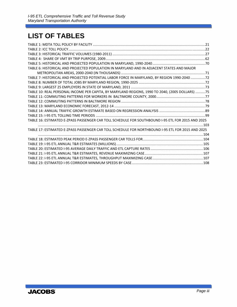
LIST OF TABLES TABLE 1: MDTA TOLL POLICY BY FACILITY ................................................................................................................... 21 TABLE 2: ICC TOLL POLICY ............................................................................................................................................ 22 TABLE 3: HISTORICAL TRAFFIC VOLUMES (1980‐2011) ............................................................................................... 27 TABLE 4: SHARE OF VMT BY TRIP PURPOSE, 2009 ...................................................................................................... 62 TABLE 5: HISTORICAL AND PROJECTED POPULATION IN MARYLAND, 1990‐2040 ...................................................... 70 TABLE 6: HISTORICAL AND PROJECTED POPULATION IN MARYLAND AND IN ADJACENT STATES AND MAJOR
METROPOLITAN AREAS, 2000‐2040 (IN THOUSANDS) ...................................................................................... 71 TABLE 7: HISTORICAL AND PROJECTED POTENTIAL LABOR FORCE IN MARYLAND, BY REGION 1990‐2040 ............... 72 TABLE 8: NUMBER OF TOTAL JOBS BY MARYLAND REGION, 1990‐2025 .................................................................... 72 TABLE 9: LARGEST 25 EMPLOYERS IN STATE OF MARYLAND, 2011 ............................................................................ 73 TABLE 10: REAL PERSONAL INCOME PER CAPITA, BY MARYLAND REGIONS, 1990 TO 2040, (2005 DOLLARS) .......... 75 TABLE 11: COMMUTING PATTERNS FOR WORKERS IN BALTIMORE COUNTY, 2000 .................................................. 77 TABLE 12: COMMUTING PATTERNS IN BALTIMORE REGION ...................................................................................... 78 TABLE 13: MARYLAND ECONOMIC FORECAST, 2012‐14 ............................................................................................. 79 TABLE 14: ANNUAL TRAFFIC GROWTH ESTIMATE BASED ON REGRESSION ANALYSIS ............................................... 89 TABLE 15: I‐95 ETL TOLLING TIME PERIODS ................................................................................................................ 99 TABLE 16: ESTIMATED E‐ZPASS PASSENGER CAR TOLL SCHEDULE FOR SOUTHBOUND I‐95 ETL FOR 2015 AND 2025
......................................................................................................................................................................... 103 TABLE 17: ESTIMATED E‐ZPASS PASSENGER CAR TOLL SCHEDULE FOR NORTHBOUND I‐95 ETL FOR 2015 AND 2025
......................................................................................................................................................................... 104 TABLE 18: ESTIMATED PEAK PERIOD E‐ZPASS PASSENGER CAR TOLLS FOR .............................................................. 104 TABLE 19: I‐95 ETL ANNUAL T&R ESTIMATES (MILLIONS) ......................................................................................... 105 TABLE 20: ESTIMATED I‐95 AVERAGE DAILY TRAFFIC AND ETL CAPTURE RATES ...................................................... 106 TABLE 21: I‐95 ETL ANNUAL T&R ESTIMATES, REVENUE MAXIMIZING CASE ............................................................ 107 TABLE 22: I‐95 ETL ANNUAL T&R ESTIMATES, THROUGHPUT MAXIMIZING CASE .................................................... 107 TABLE 23: ESTIMATED I‐95 CORRIDOR MINIMUM SPEEDS BY CASE ......................................................................... 108
I-95 ETL Comprehensive Traffic and Toll Revenue Study Maryland Transportation Authority
Page iv
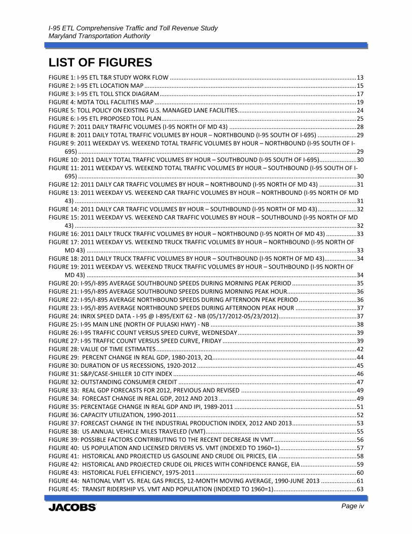
LIST OF FIGURES FIGURE 1: I‐95 ETL T&R STUDY WORK FLOW .............................................................................................................. 13 FIGURE 2: I‐95 ETL LOCATION MAP ............................................................................................................................. 15 FIGURE 3: I‐95 ETL TOLL STICK DIAGRAM .................................................................................................................... 17 FIGURE 4: MDTA TOLL FACILITIES MAP ....................................................................................................................... 19 FIGURE 5: TOLL POLICY ON EXISTING U.S. MANAGED LANE FACILITIES ...................................................................... 24 FIGURE 6: I‐95 ETL PROPOSED TOLL PLAN ................................................................................................................... 25 FIGURE 7: 2011 DAILY TRAFFIC VOLUMES (I‐95 NORTH OF MD 43) ........................................................................... 28 FIGURE 8: 2011 DAILY TOTAL TRAFFIC VOLUMES BY HOUR – NORTHBOUND (I‐95 SOUTH OF I‐695) ....................... 29 FIGURE 9: 2011 WEEKDAY VS. WEEKEND TOTAL TRAFFIC VOLUMES BY HOUR – NORTHBOUND (I‐95 SOUTH OF I‐
695) .................................................................................................................................................................... 29 FIGURE 10: 2011 DAILY TOTAL TRAFFIC VOLUMES BY HOUR – SOUTHBOUND (I‐95 SOUTH OF I‐695) ...................... 30 FIGURE 11: 2011 WEEKDAY VS. WEEKEND TOTAL TRAFFIC VOLUMES BY HOUR – SOUTHBOUND (I‐95 SOUTH OF I‐
695) .................................................................................................................................................................... 30 FIGURE 12: 2011 DAILY CAR TRAFFIC VOLUMES BY HOUR – NORTHBOUND (I‐95 NORTH OF MD 43) ...................... 31 FIGURE 13: 2011 WEEKDAY VS. WEEKEND CAR TRAFFIC VOLUMES BY HOUR – NORTHBOUND (I‐95 NORTH OF MD
43) ...................................................................................................................................................................... 31 FIGURE 14: 2011 DAILY CAR TRAFFIC VOLUMES BY HOUR – SOUTHBOUND (I‐95 NORTH OF MD 43) ....................... 32 FIGURE 15: 2011 WEEKDAY VS. WEEKEND CAR TRAFFIC VOLUMES BY HOUR – SOUTHBOUND (I‐95 NORTH OF MD
43) ...................................................................................................................................................................... 32 FIGURE 16: 2011 DAILY TRUCK TRAFFIC VOLUMES BY HOUR – NORTHBOUND (I‐95 NORTH OF MD 43) .................. 33 FIGURE 17: 2011 WEEKDAY VS. WEEKEND TRUCK TRAFFIC VOLUMES BY HOUR – NORTHBOUND (I‐95 NORTH OF
MD 43) ............................................................................................................................................................... 33 FIGURE 18: 2011 DAILY TRUCK TRAFFIC VOLUMES BY HOUR – SOUTHBOUND (I‐95 NORTH OF MD 43) ................... 34 FIGURE 19: 2011 WEEKDAY VS. WEEKEND TRUCK TRAFFIC VOLUMES BY HOUR – SOUTHBOUND (I‐95 NORTH OF
MD 43) ............................................................................................................................................................... 34 FIGURE 20: I‐95/I‐895 AVERAGE SOUTHBOUND SPEEDS DURING MORNING PEAK PERIOD ...................................... 35 FIGURE 21: I‐95/I‐895 AVERAGE SOUTHBOUND SPEEDS DURING MORNING PEAK HOUR ......................................... 36 FIGURE 22: I‐95/I‐895 AVERAGE NORTHBOUND SPEEDS DURING AFTERNOON PEAK PERIOD .................................. 36 FIGURE 23: I‐95/I‐895 AVERAGE NORTHBOUND SPEEDS DURING AFTERNOON PEAK HOUR .................................... 37 FIGURE 24: INRIX SPEED DATA ‐ I‐95 @ I‐895/EXIT 62 ‐ NB (05/17/2012‐05/23/2012) .............................................. 37 FIGURE 25: I‐95 MAIN LINE (NORTH OF PULASKI HWY) ‐ NB ...................................................................................... 38 FIGURE 26: I‐95 TRAFFIC COUNT VERSUS SPEED CURVE, WEDNESDAY ...................................................................... 39 FIGURE 27: I‐95 TRAFFIC COUNT VERSUS SPEED CURVE, FRIDAY ............................................................................... 39 FIGURE 28: VALUE OF TIME ESTIMATES ...................................................................................................................... 42 FIGURE 29: PERCENT CHANGE IN REAL GDP, 1980‐2013, 2Q ..................................................................................... 44 FIGURE 30: DURATION OF US RECESSIONS, 1920‐2012 .............................................................................................. 45 FIGURE 31: S&P/CASE‐SHILLER 10 CITY INDEX ............................................................................................................ 46 FIGURE 32: OUTSTANDING CONSUMER CREDIT ......................................................................................................... 47 FIGURE 33: REAL GDP FORECASTS FOR 2012, PREVIOUS AND REVISED .................................................................... 49 FIGURE 34: FORECAST CHANGE IN REAL GDP, 2012 AND 2013 ................................................................................. 49 FIGURE 35: PERCENTAGE CHANGE IN REAL GDP AND IPI, 1989‐2011 ........................................................................ 51 FIGURE 36: CAPACITY UTILIZATION, 1990‐2011 .......................................................................................................... 52 FIGURE 37: FORECAST CHANGE IN THE INDUSTRIAL PRODUCTION INDEX, 2012 AND 2013 ...................................... 53 FIGURE 38: US ANNUAL VEHICLE MILES TRAVELED (VMT) ......................................................................................... 55 FIGURE 39: POSSIBLE FACTORS CONTRIBUTING TO THE RECENT DECREASE IN VMT ................................................. 56 FIGURE 40: US POPULATION AND LICENSED DRIVERS VS. VMT (INDEXED TO 1960=1) ............................................. 57 FIGURE 41: HISTORICAL AND PROJECTED US GASOLINE AND CRUDE OIL PRICES, EIA .............................................. 58 FIGURE 42: HISTORICAL AND PROJECTED CRUDE OIL PRICES WITH CONFIDENCE RANGE, EIA ................................. 59 FIGURE 43: HISTORICAL FUEL EFFICIENCY, 1975‐2011 ............................................................................................... 60 FIGURE 44: NATIONAL VMT VS. REAL GAS PRICES, 12‐MONTH MOVING AVERAGE, 1990‐JUNE 2013 ..................... 61 FIGURE 45: TRANSIT RIDERSHIP VS. VMT AND POPULATION (INDEXED TO 1960=1) ................................................. 63

I-95 ETL Comprehensive Traffic and Toll Revenue Study Maryland Transportation Authority
Page v
FIGURE 46: TRANSIT PMT VS. HIGHWAY VMT (INDEXED TO 1995=1) ........................................................................ 64 FIGURE 47: US POPULATION DISTRIBUTION BY AGE GROUP ..................................................................................... 66 FIGURE 48: AVERAGE VMT PER PERSON BY AGE RANGE, 2009 ................................................................................. 67 FIGURE 49: PARTICIPATION IN THE WORKFORCE BY GENDER ................................................................................... 68 FIGURE 50: CHANGE IN REAL GDP BY STATE IN THE MIDEAST REGION FOR 2012 ...................................................... 69 FIGURE 51: BALTIMORE MSA, MARYLAND AND NATIONAL UNEMPLOYMENT RATES, 1998 TO JUNE 2013 .............. 74 FIGURE 52: MEDIAN HOUSEHOLD INCOME, 2010$ .................................................................................................... 76 FIGURE 53: I‐95 ETL MODELING METHODOLOGY FLOW CHART ................................................................................. 82 FIGURE 54: I‐95 ETL T&R STUDY BASIC ASSUMPTIONS ............................................................................................... 86 FIGURE 55: I‐95 ETL TOLL STICK DIAGRAM .................................................................................................................. 87 FIGURE 56: HISTORICAL TRAFFIC AND LINEAR REGRESSION BY YEAR ......................................................................... 89 FIGURE 57: I‐95 HISTORICAL AND FORECASTED CORRIDOR DEMAND AT ETL TOLL GANTRY ..................................... 90 FIGURE 58: NORTHBOUND HALF‐HOUR PROFILES BY DAY OF THE WEEK .................................................................. 91 FIGURE 59: SOUTHBOUND HALF‐HOUR PROFILES BY DAY OF THE WEEK ................................................................... 91 FIGURE 60: ETL HOURLY TRAFFIC VOLUMES AS A FUNCTION OF TOLL RATE AND CORRIDOR DEMAND ................... 94 FIGURE 61: ETL HOURLY TOLL REVENUE AS A FUNCTION OF TOLL RATE AND CORRIDOR DEMAND ......................... 95 FIGURE 62: MAXIMUM HOURLY CAR TOLL REVENUE AS A FUNCTION CORRIDOR DEMAND ..................................... 96 FIGURE 63: ETL HOURLY TRUCK TRAFFIC VOLUMES AS A FUNCTION OF 5 AXLE TRUCK TOLL RATE AND CORRIDOR
DEMAND ............................................................................................................................................................ 97 FIGURE 64: ETL HOURLY TRUCK TOLL REVENUE AS A FUNCTION OF 5 AXLE TRUCK TOLL RATE AND CORRIDOR
DEMAND ............................................................................................................................................................ 98 FIGURE 65: MAXIMUM HOURLY TRUCK TOLL REVENUE AS A FUNCTION CORRIDOR DEMAND ................................. 98 FIGURE 66: I‐95 ETL TOLL SENSITIVITY, WEEKDAY PEAK, 2015 ................................................................................. 100 FIGURE 67: I‐95 ETL TOLL SENSITIVITY, WEEKDAY OFF‐PEAK, 2015 .......................................................................... 100 FIGURE 68: I‐95 ETL TOLL SENSITIVITY, WEEKEND PEAK, 2015 ................................................................................. 101 FIGURE 69: I‐95 ETL TOLL SENSITIVITY, WEEKEND OFF‐PEAK, 2015 .......................................................................... 101 FIGURE 70: I‐95 ETL TOLL SENSITIVITY, OVERNIGHT, 2015 ....................................................................................... 102 FIGURE 71: I‐95 ETL ANNUAL T&R ESTIMATES (MILLIONS) ....................................................................................... 105 FIGURE 72: I‐95 ETL TOLL REVENUE FORECAST RISK ANALYSIS ................................................................................. 110
I-95 ETL Comprehensive Traffic and Toll Revenue Study Maryland Transportation Authority
Page 1
Executive Summary The Maryland Transportation Authority (MDTA) retained Jacobs Engineering Group (Jacobs) to develop traffic and toll revenue estimates for the Express Toll Lanes (ETL) constructed as part of the I-95 Improvement Project. Jacobs’ assignment was to quantify traffic volumes, prepare potential appropriate toll rate ranges1 and specific toll rates reflecting traffic demand and operational goals, and to project anticipated revenues for the I-95 ETL, based on these potential toll rates. It is important to note that the toll rates which form the basis of the revenue projections included in this study are recommendations. The actual toll rates to be used are yet to be determined by MDTA and could differ from those used in this study. Accordingly, revenues could differ from those predicted. Actual traffic experience will ultimately determine the toll rates used to manage traffic volumes. MDTA currently operates eight toll facilities within the State of Maryland consisting of two expressways, two tunnels and four bridges that provide critical transportation infrastructure links for both local and regional movement of people and goods. The John F. Kennedy Memorial Highway, one of the expressways the MDTA operates, is a 50-mile section of I-95 from the northeastern Baltimore City line to Delaware. Currently tolls are collected one mile north of the Millard E. Tydings Memorial Bridge over the Susquehanna River in northeastern Maryland in the northbound direction only. This stretch of roadway serves local and regional travel as both a conduit for commuters from areas north of Baltimore into Baltimore City and for longer distance trips for both personal and commercial vehicles as part of the I-95 corridor that stretches from Maine to Florida. The I-95 ETL is constructed as part of a series of improvements to I-95 northeast of Baltimore intended to improve safety and reduce congestion. In its current configuration, the ETL extends approximately 8 miles within the median of I-95. (Potential future northward extensions of the project are not considered in this report.) The shortest travel distance on the facility is between MD 43 and Moravia Road, therefore this distance, 7 miles, is used to calculate toll rates. The full ETL stretches from north of MD 43 to south of the split of I-95 and I-895, south of Pulaski Highway and Moravia Road, respectively. The I-95 ETL will operate as a price-managed toll facility with similar features to many other express toll lane facilities throughout the United States such as along a portion of the Capital Beltway in the Washington D.C. area. The distinguishing feature of a price-
1 On its variable priced facilities (the Intercounty Connector and the ETL project) MDTA sets toll rate ranges which define the lower and upper limits of potential toll rates that can be used to manage demand and congestion on the facilities. The MDTA Executive Secretary then sets, and can subsequently adjust, specific toll rates, provided that they remain within the approved toll rate range.
I-95 ETL Comprehensive Traffic and Toll Revenue Study Maryland Transportation Authority
Page 2
managed toll facility is the control of traffic levels through toll rates. One goal of the I-95 ETL is to provide reliable travel time for motorists. To achieve this goal, the MDTA will charge different levels of tolls depending on the traffic demand in the corridor, which changes over the course of a day and is different by day of the week as well. In the AM period the southbound direction experiences very heavy traffic. This requires a toll that is higher than the off-peak time period to achieve a consistent travel time in the ETL. The introduction of additional toll-free general purpose lanes in congested, growing areas, while often offering a short-term solution to traffic delay, typically does not reduce congestion in the long term. Managed lane facilities, on the other hand, provide a long-term option for a congestion-free trip using pricing to provide motorists reliable travel times at a market-driven toll rate. A standard work flow of traffic and toll revenue forecasting for managed lanes was employed to forecast traffic and toll revenue as well as develop toll schedules appropriate to manage traffic demand. First, basic assumptions were developed and documented. Then data was collected regarding motorists’ current travel patterns and willingness to pay, historical traffic data, socioeconomic data in the corridor, and projected traffic and traffic patterns in the corridor. These data were used as input into multiple modeling platforms to provide forecasted traffic volumes in the corridor, operational characteristics of the corridor, toll schedules needed to manage peak and off-peak traffic and finally traffic and toll revenue estimates. Multiple sensitivity tests were run within those multiple models to quantify overall risk to revenue projections. In undertaking this work, MDTA staff and Jacobs have assumed that toll rates for the ETL would be set at a level which would regulate demand for the ETL so that ETL users could operate at or near 55 mph. (For a complete list of the basic T&R study assumptions, see Table ES-2.) When traffic volume in adjacent untolled lanes is generally light and uncongested, fewer people would be willing to use the ETL lanes, thus, toll rates are accordingly lower at those times of day. When traffic volume in adjacent untolled lanes is generally higher and more congested, more drivers are willing to use the ETL lanes, thus, toll rates in the ETL lanes are accordingly higher at those times of day, thus regulating the number of persons who will choose to use the ETL, and thus maintaining a congestion free 55 mph operating speed in the ETL. Existing traffic conditions in the corridor provide an empirical snapshot of how traffic functions today. This combined with the historical experience in the corridor, year over year, and forecasted traffic volumes provide key input into the traffic and toll revenue forecasting model.
I-95 ETL Comprehensive Traffic and Toll Revenue Study Maryland Transportation Authority
Page 3
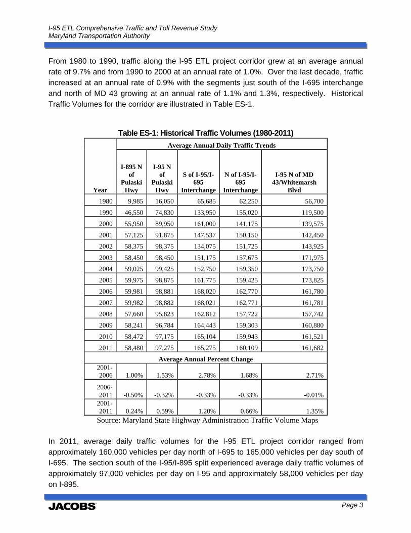
From 1980 to 1990, traffic along the I-95 ETL project corridor grew at an average annual rate of 9.7% and from 1990 to 2000 at an annual rate of 1.0%. Over the last decade, traffic increased at an annual rate of 0.9% with the segments just south of the I-695 interchange and north of MD 43 growing at an annual rate of 1.1% and 1.3%, respectively. Historical Traffic Volumes for the corridor are illustrated in Table ES-1.
Table ES-1: Historical Traffic Volumes (1980-2011)
Year
Average Annual Daily Traffic Trends
I-895 N of
Pulaski Hwy
I-95 N of
Pulaski Hwy
S of I-95/I-695
Interchange
N of I-95/I-695
Interchange
I-95 N of MD 43/Whitemarsh
Blvd
1980 9,985 16,050 65,685 62,250 56,700
1990 46,550 74,830 133,950 155,020 119,500
2000 55,950 89,950 161,000 141,175 139,575
2001 57,125 91,875 147,537 150,150 142,450
2002 58,375 98,375 134,075 151,725 143,925
2003 58,450 98,450 151,175 157,675 171,975
2004 59,025 99,425 152,750 159,350 173,750
2005 59,975 98,875 161,775 159,425 173,825
2006 59,981 98,881 168,020 162,770 161,780
2007 59,982 98,882 168,021 162,771 161,781
2008 57,660 95,823 162,812 157,722 157,742
2009 58,241 96,784 164,443 159,303 160,880
2010 58,472 97,175 165,104 159,943 161,521
2011 58,480 97,275 165,275 160,109 161,682
Average Annual Percent Change 2001-2006 1.00% 1.53% 2.78% 1.68% 2.71%
2006-2011 -0.50% -0.32% -0.33% -0.33% -0.01%
2001-2011 0.24% 0.59% 1.20% 0.66% 1.35%
Source: Maryland State Highway Administration Traffic Volume Maps In 2011, average daily traffic volumes for the I-95 ETL project corridor ranged from approximately 160,000 vehicles per day north of I-695 to 165,000 vehicles per day south of I-695. The section south of the I-95/I-895 split experienced average daily traffic volumes of approximately 97,000 vehicles per day on I-95 and approximately 58,000 vehicles per day on I-895.
I-95 ETL Comprehensive Traffic and Toll Revenue Study Maryland Transportation Authority
Page 4
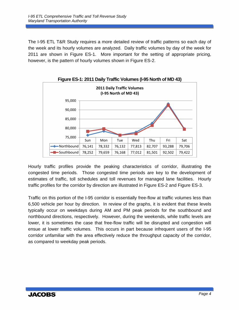
The I-95 ETL T&R Study requires a more detailed review of traffic patterns so each day of the week and its hourly volumes are analyzed. Daily traffic volumes by day of the week for 2011 are shown in Figure ES-1. More important for the setting of appropriate pricing, however, is the pattern of hourly volumes shown in Figure ES-2.
Figure ES-1: 2011 Daily Traffic Volumes (I-95 North of MD 43)
Hourly traffic profiles provide the peaking characteristics of corridor, illustrating the congested time periods. Those congested time periods are key to the development of estimates of traffic, toll schedules and toll revenues for managed lane facilities. Hourly traffic profiles for the corridor by direction are illustrated in Figure ES-2 and Figure ES-3. Traffic on this portion of the I-95 corridor is essentially free-flow at traffic volumes less than 6,500 vehicle per hour by direction. In review of the graphs, it is evident that these levels typically occur on weekdays during AM and PM peak periods for the southbound and northbound directions, respectively. However, during the weekends, while traffic levels are lower, it is sometimes the case that free-flow traffic will be disrupted and congestion will ensue at lower traffic volumes. This occurs in part because infrequent users of the I-95 corridor unfamiliar with the area effectively reduce the throughput capacity of the corridor, as compared to weekday peak periods.
Sun Mon Tue Wed Thu Fri Sat
Northbound 76,141 78,332 76,132 77,813 82,707 93,288 79,706
Southbound 78,252 79,659 76,168 77,012 81,501 92,502 79,422
75,000
80,000
85,000
90,000
95,000
2011 Daily Traffic Volumes (I‐95 North of MD 43)

I-95 ETL Comprehensive Traffic and Toll Revenue Study Maryland Transportation Authority
Page 5
Figure ES-2: 2011 Daily Total Traffic Volumes by Hour – Northbound (I-95 South of I-695)
Figure ES-3: 2011 Daily Total Traffic Volumes by Hour – Southbound (I-95 South of I-695)
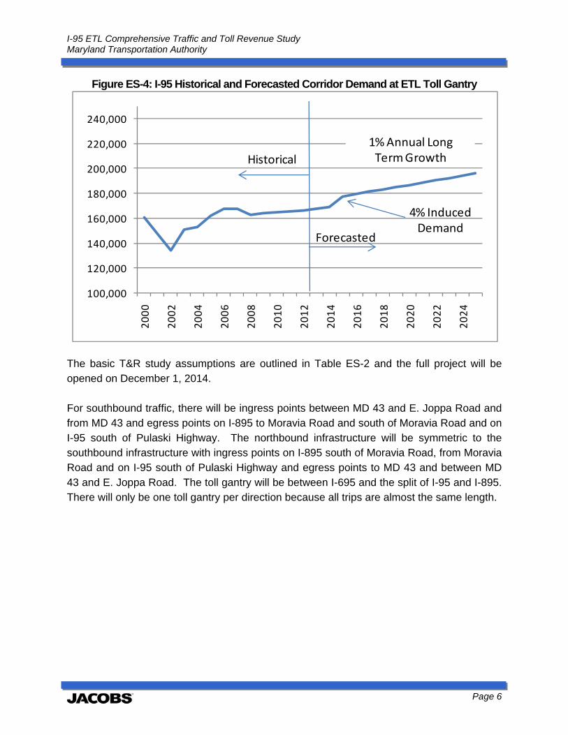
Figure ES-4 presents the historical and projected average daily traffic volumes on I-95 south of I-695 after completion of the I-95 improvement project including the ETL. The induced demand attracted by the additional capacity in the corridor is estimated to create a one-time 4 percent increase in traffic in addition to the projected long-term traffic growth rate of one percent.
0
1,000
2,000
3,000
4,000
5,000
6,000
7,000
8,000
0:00 2:00 4:00 6:00 8:00 10:0012:0014:0016:0018:0020:0022:00
2011 Daily Volumes by Hour ‐Northbound (I‐95 South of I‐695)
Sun
Mon
Tue
Wed
Thu
Fri
Sat
0
1,000
2,000
3,000
4,000
5,000
6,000
7,000
8,000
0:00 2:00 4:00 6:00 8:00 10:0012:0014:0016:0018:0020:0022:00
2011 Daily Volumes by Hour‐ Southbound (I‐95 South of I‐695)
Sun
Mon
Tue
Wed
Thu
Fri
Sat
I-95 ETL Comprehensive Traffic and Toll Revenue Study Maryland Transportation Authority
Page 6
Figure ES-4: I-95 Historical and Forecasted Corridor Demand at ETL Toll Gantry
The basic T&R study assumptions are outlined in Table ES-2 and the full project will be opened on December 1, 2014. For southbound traffic, there will be ingress points between MD 43 and E. Joppa Road and from MD 43 and egress points on I-895 to Moravia Road and south of Moravia Road and on I-95 south of Pulaski Highway. The northbound infrastructure will be symmetric to the southbound infrastructure with ingress points on I-895 south of Moravia Road, from Moravia Road and on I-95 south of Pulaski Highway and egress points to MD 43 and between MD 43 and E. Joppa Road. The toll gantry will be between I-695 and the split of I-95 and I-895. There will only be one toll gantry per direction because all trips are almost the same length.
100,000
120,000
140,000
160,000
180,000
200,000
220,000
240,000
2000
2002
2004
2006
2008
2010
2012
2014
2016
2018
2020
2022
2024
Historical
Forecasted
4% Induced Demand
1%Annual Long Term Growth
I-95 ETL Comprehensive Traffic and Toll Revenue Study Maryland Transportation Authority
Page 7
Table ES-2: I-95 ETL T&R Study Basic Assumptions
The forecasting of traffic, toll schedules, and toll revenue for managed lane facilities requires the use of multiple forecasting models on multiple modeling platforms. This analysis uses the Baltimore Metropolitan Council travel demand model (BMC Model), the I-95 ETL VISSIM micro-simulation model (VISSIM model) and the I-95 ETL traffic, toll schedule and toll revenue forecasting model (T&R Model). Multiple tolling periods and toll rates within those periods were analyzed including the use of shoulder peak toll rates for time periods between the heights of the peak period and off-peak. Time increments were disaggregated to the half hour to estimate needed toll rates and resulting operations under a changing toll rate every half hour. Through the course of the analysis, it was evident toll rates needed to manage traffic in the peak time periods were
Assumption
InfrastructureProject Limits/Access Points/Typical Section See Stick DiagramsLength 7 milesOpening Date 12/1/2014
Toll Policy
Toll CollectionAll Electronic Toll Collection (AETC) with E-ZPass and Video Toll (No Cash Collection)
2 axle Base Toll Rate (E-ZPass)
As needed to manage congestion by time period using ICC toll rate ranges (distance * mileage rate for pre-determined pricing periods)
2 axle Video Toll Rate50% surcharge on base rate with $1 minimum and $15 maximum surcharges
Toll EscalationThere is no annual toll escalation, only escalation based on the need to manage traffic in the peak periods
Congestion PricingPre-determined time-of-day pricing intended to maintain 55 mph in the ETL, adjustable with ten days notice
Axle Multiplier from 2 axleBased on Current MDTA policy on ICC, which is different than the current policy at the JFK toll plaza
AssumptionCorridor Demand Adjusted TDM results, following BHT, FMT and JFK forecastsValue of Time $7.79 to $16.90 per hour by Hour and Payment TypeHourly Traffic Profile By Day of Week from 2011 permanent count stationPercentage of Video 5-10% by HourPercentage of Trucks Corridor Rate by Day of Week and Hour (6% to 30%)Ramp-up 2 years, 85%, 95%Axle Factor Corridor Rate by Day of Week and Hour (3.1 to 4.7)Violation Rates 2% for Transponders; 20% for VideoAnnualization Factor Modeled Days of Week Individually (each times 52)Holiday Schedules Not accounted for in the T&R Estimates
Lane Capacity (a function of driver familiarity)Monday - Thursday 1800 vplphFriday, Saturday, Sunday 1750 vplph
Assumptions for I-95 T&R Study - Operator ControlledVariable
Assumptions for I-95 T&R Study - Market DrivenVariable
I-95 ETL Comprehensive Traffic and Toll Revenue Study Maryland Transportation Authority
Page 8
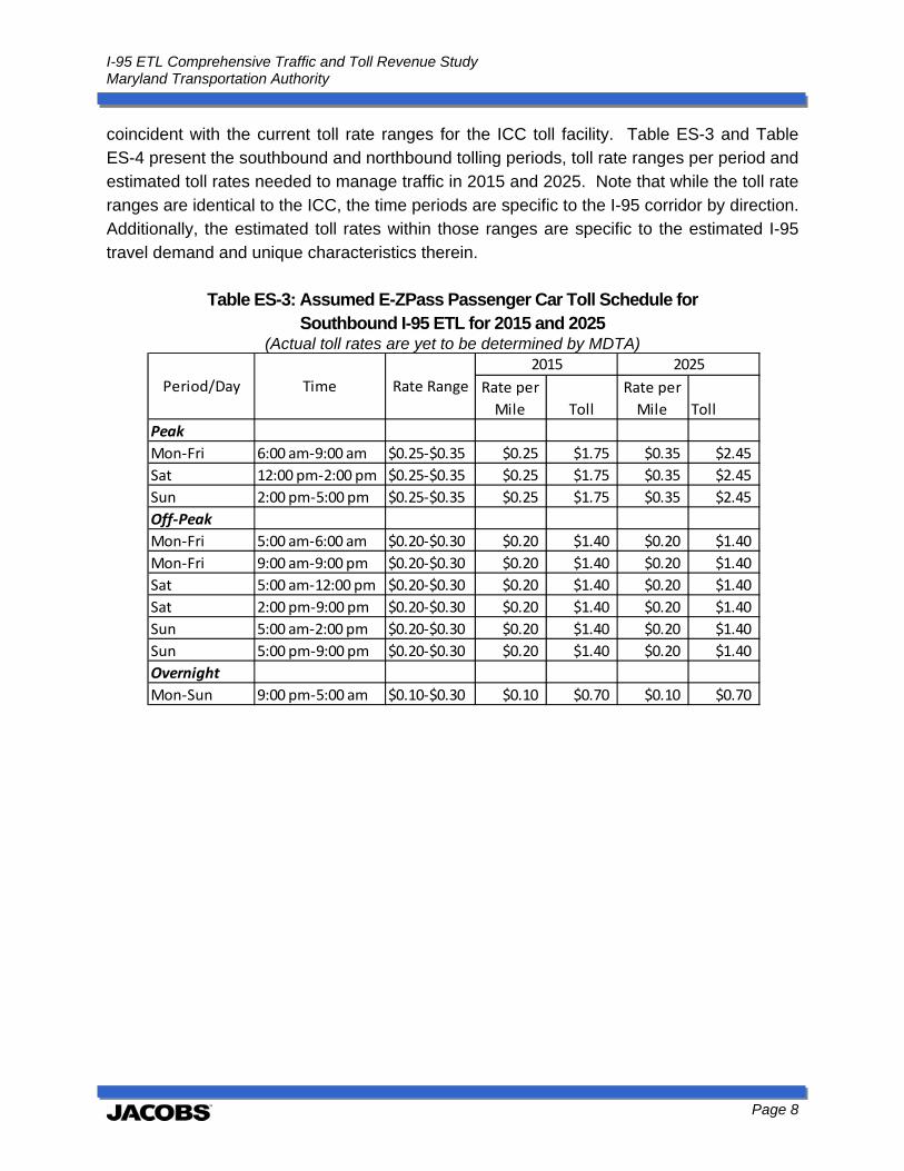
coincident with the current toll rate ranges for the ICC toll facility. Table ES-3 and Table ES-4 present the southbound and northbound tolling periods, toll rate ranges per period and estimated toll rates needed to manage traffic in 2015 and 2025. Note that while the toll rate ranges are identical to the ICC, the time periods are specific to the I-95 corridor by direction. Additionally, the estimated toll rates within those ranges are specific to the estimated I-95 travel demand and unique characteristics therein.
Table ES-3: Assumed E-ZPass Passenger Car Toll Schedule for Southbound I-95 ETL for 2015 and 2025
(Actual toll rates are yet to be determined by MDTA)
Rate per
Mile Toll
Rate per
Mile Toll
Peak
Mon‐Fri 6:00 am‐9:00 am $0.25‐$0.35 $0.25 $1.75 $0.35 $2.45
Sat 12:00 pm‐2:00 pm $0.25‐$0.35 $0.25 $1.75 $0.35 $2.45
Sun 2:00 pm‐5:00 pm $0.25‐$0.35 $0.25 $1.75 $0.35 $2.45
Off‐Peak
Mon‐Fri 5:00 am‐6:00 am $0.20‐$0.30 $0.20 $1.40 $0.20 $1.40
Mon‐Fri 9:00 am‐9:00 pm $0.20‐$0.30 $0.20 $1.40 $0.20 $1.40
Sat 5:00 am‐12:00 pm $0.20‐$0.30 $0.20 $1.40 $0.20 $1.40
Sat 2:00 pm‐9:00 pm $0.20‐$0.30 $0.20 $1.40 $0.20 $1.40
Sun 5:00 am‐2:00 pm $0.20‐$0.30 $0.20 $1.40 $0.20 $1.40
Sun 5:00 pm‐9:00 pm $0.20‐$0.30 $0.20 $1.40 $0.20 $1.40
Overnight
Mon‐Sun 9:00 pm‐5:00 am $0.10‐$0.30 $0.10 $0.70 $0.10 $0.70
Period/Day Time Rate Range
2015 2025

I-95 ETL Comprehensive Traffic and Toll Revenue Study Maryland Transportation Authority
Page 9
Table ES-4: Assumed E-ZPass Passenger Car Toll Schedule for Northbound I-95 ETL for 2015 and 2025
(Actual toll rates are yet to be determined by MDTA)
During the forecast period it is estimated that only peak period toll rates will need to be increased to manage traffic levels and the maximum toll rates will be needed by 2023. Table ES-5 presents the estimated peak period tolls from 2015 to 2025. The analysis indicated that peak period toll rates would need to be adjusted about four times beginning in 2020.
Table ES-5: Estimated Peak Period E-ZPass Passenger Car Tolls for I-95 ETL, 2015 to 2025
Rate per
Mile Toll
Rate per
Mile Toll
Peak
Mon‐Fri 6:00 am‐9:00 am $0.25‐$0.35 $0.25 $1.75 $0.35 $2.45
Sat 12:00 pm‐2:00 pm $0.25‐$0.35 $0.25 $1.75 $0.35 $2.45
Sun 2:00 pm‐5:00 pm $0.25‐$0.35 $0.25 $1.75 $0.35 $2.45
Off‐Peak
Mon‐Fri 5:00 am‐6:00 am $0.20‐$0.30 $0.20 $1.40 $0.20 $1.40
Mon‐Fri 9:00 am‐9:00 pm $0.20‐$0.30 $0.20 $1.40 $0.20 $1.40
Sat 5:00 am‐12:00 pm $0.20‐$0.30 $0.20 $1.40 $0.20 $1.40
Sat 2:00 pm‐9:00 pm $0.20‐$0.30 $0.20 $1.40 $0.20 $1.40
Sun 5:00 am‐2:00 pm $0.20‐$0.30 $0.20 $1.40 $0.20 $1.40
Sun 5:00 pm‐9:00 pm $0.20‐$0.30 $0.20 $1.40 $0.20 $1.40
Overnight
Mon‐Sun 9:00 pm‐5:00 am $0.10‐$0.30 $0.10 $0.70 $0.10 $0.70
Period/Day Time Rate Range
2015 2025
Year Peak Period Toll
2015 $1.75
2016 $1.75
2017 $1.75
2018 $1.75
2019 $1.75
2020 $1.90
2021 $2.05
2022 $2.15
2023 $2.45
2024 $2.45
2025 $2.45
I-95 ETL Comprehensive Traffic and Toll Revenue Study Maryland Transportation Authority
Page 10
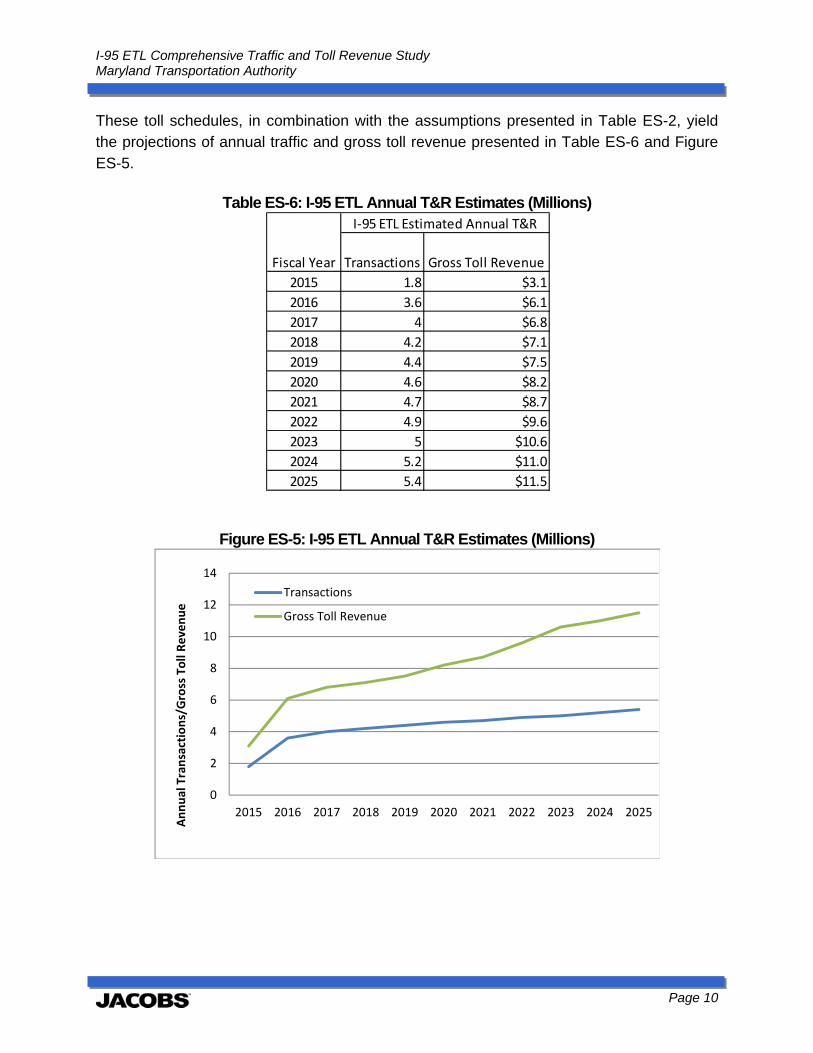
These toll schedules, in combination with the assumptions presented in Table ES-2, yield the projections of annual traffic and gross toll revenue presented in Table ES-6 and Figure ES-5.
Table ES-6: I-95 ETL Annual T&R Estimates (Millions)
Figure ES-5: I-95 ETL Annual T&R Estimates (Millions)
Transactions Gross Toll Revenue
2015 1.8 $3.1
2016 3.6 $6.1
2017 4 $6.8
2018 4.2 $7.1
2019 4.4 $7.5
2020 4.6 $8.2
2021 4.7 $8.7
2022 4.9 $9.6
2023 5 $10.6
2024 5.2 $11.0
2025 5.4 $11.5
Fiscal Year
I‐95 ETL Estimated Annual T&R
0
2
4
6
8
10
12
14
2015 2016 2017 2018 2019 2020 2021 2022 2023 2024 2025
Annual Transactions/Gross Toll Revenue
Transactions
Gross Toll Revenue
I-95 ETL Comprehensive Traffic and Toll Revenue Study Maryland Transportation Authority
Page 11
1.0 Introduction The Maryland Transportation Authority (MDTA) currently operates eight toll facilities within the State of Maryland consisting of two expressways, two tunnels and four bridges that provide critical transportation infrastructure links for both local and regional movement of people and goods. The John F. Kennedy Memorial Highway, one of the expressways the MDTA operates, is a 50-mile section of I-95 from the northern Baltimore City line to Delaware. Currently, tolls are collected one mile north of the Millard E.Tydings Memorial Bridge over the Susquehanna River in northeast Maryland in the northbound direction only. This stretch of roadway caters to both local and regional travel as both a conduit for commuters from areas north of Baltimore into Baltimore City and longer distance trips for both personal and commercial vehicles as part of the I-95 corridor that stretches from Maine to Florida. The I-95 ETL is constructed as part of a series of improvements to I-95 northeast of Baltimore intended to improve safety and reduce congestion. The ETL extends approximately 8 miles within the median of I-95. The shortest travel distance on the facility is between MD 43 and Moravia Road, therefore this distance, 7 miles, is used to calculate toll rates. The full ETL stretches from north of MD 43 to south of the split of I-95 and I-895, south of Pulaski Highway and Moravia Road, respectively. Jacobs Engineering Group (Jacobs) was retained by the MDTA to develop traffic and toll revenue estimates for the I-95 ETL, quantifying traffic, toll schedules and toll revenue. In this section, the purpose and scope of the analysis is further explored, the methodology to complete that analysis is explained, the outline of the presentation of the analysis as contained in this report is provided including a more detailed description of the I-95 ETL project.
1.1 Study Purpose and Scope The I-95 ETL will operate as a price-managed toll facility with similar features to many other express toll lane facilities throughout the United States such as the Capital Beltway in the Washington D.C. area. The distinguishing feature of a price-managed toll facility is the control of traffic levels through toll rates. One goal of the I-95 ETL is to provide reliable travel time for motorists. In order to achieve this goal, the MDTA will charge different levels of tolls depending on the traffic demand in the corridor, which changes over the course of a day and is different by day of the week as well. In the AM period the southbound direction experiences very heavy traffic. This requires a toll that is higher than the off-peak time period to achieve a consistent travel time in the ETL.
I-95 ETL Comprehensive Traffic and Toll Revenue Study Maryland Transportation Authority
Page 12
Jacobs was tasked with developing projections of traffic and toll revenue for the I-95 ETL for a forecast period of 10 years. Based on the nature of managed toll facilities, a significant part of the analysis within a traffic and toll revenue study is to develop appropriate time-of-day toll schedules to manage traffic levels on the ETL that provide reliable travel times on both opening day and the 10th year of the forecast. The following section describes the process by which the traffic, toll revenue and toll schedules are developed in a logical, linear manner.
1.2 Study Methodology A standard work flow of traffic and toll revenue forecasting for managed lanes was employed to forecast traffic and toll revenue as well as develop toll schedules appropriate to manage traffic demand. Figure 1 presents a simplified version of the work flow. The first step was to develop some basic assumptions including what the project would look like once built, what the tolling policy would be and what are the factors that would determine motorists’ usage of the lanes at given toll rates. The first two sets of assumptions were developed by MDTA with input from Jacobs and the final set of assumptions, those that determine usage of the I-95 ETL, were developed through the next step, the data collection and analysis effort. Data collection included existing traffic patterns, motorists’ willingness to pay, and socioeconomic factors. The collected data was input into the modeling processes which included the use of the Baltimore Metropolitan Council’s travel demand model (BMC Model), an I-95 ETL VISSIM micro-simulation model (traffic operation model) (VISSIM Model), and a I-95 ETL traffic, toll schedule and toll revenue model which was developed specifically for this analysis (T&R Model). The result of the modeling, which was based upon the assumptions supported by the data collection effort, was the base case traffic, toll schedule and toll revenue estimates for I-95 ETL for a 10 year period. Tests were run to understand the sensitivity of traffic and toll revenue to changes in toll rates as well as various toll policies, including those which would maximize throughput of traffic in the corridor and policies that would maximize toll revenue for the facility. In addition to sensitivity tests, a risk analysis was conducted on the base case to understand potential ranges of traffic and toll revenue as a function of consumer demand that varies from our base assumptions. The final step of the analysis was documentation of results reflected by this comprehensive traffic and toll revenue report.

I-95 ETL Comprehensive Traffic and Toll Revenue Study Maryland Transportation Authority
Page 13
Figure 1: I-95 ETL T&R Study Work Flow
1.3 Report Structure The report structure follows the study methodology and logically walks through the steps in the development of the traffic, toll revenue and toll schedules for the I-95 ETL. Section 1: Introduction, describes the I-95 ETL project, the purpose of this study and the methodology employed to complete the analysis.
AssumptionDevelopment‐Infrastructure‐Toll Policy
‐T&R Modeling
Data Collection/Analysis‐Infrastructure
‐Traffic‐Motorists'Behavior‐Socioeconomics
TravelDemand and Microsimulation Modeling
CorridorModeling Toll Rate, Traffic and Revenue Modeling
Toll Rate, Traffic and Revenue Estimates
Sensitivity Tests andRiskAnalysis
Final Documentation
I-95 ETL Comprehensive Traffic and Toll Revenue Study Maryland Transportation Authority
Page 14
Section 2: Tolling Policy, reviews the toll policies that provide the foundation for the development of the traffic, toll revenue and toll schedule estimates. First the current toll policies on existing MDTA facilities are reviewed. Then toll policies for other managed lane facilities across the United States are presented. Finally the proposed I-95 ETL toll policy is presented which combines the standard toll policies that are in effect on the MDTA existing toll facilities and the additional policies needed to provide reliable travel times on the ETL. Section 3: Corridor Traffic Conditions, reviews historical and existing traffic conditions in the I-95 corridor. These data include average annual traffic, recent daily traffic, hourly traffic and speed profiles. Additionally the relationship between traffic volume and speed in the corridor is analyzed as this is a key component of the forecasting model. Section 4: Stated Preference Survey provides a cursory review of the stated preference survey that was conducted for this analysis. The survey provides data regarding motorists’ willingness to pay as function of time savings, essentially their stated desire to trade time for money or their value of time (VOT). Motorists’ VOT is critical in determining their likelihood of paying tolls when faced with potential time savings. Section 5: Socioeconomic Conditions and Forecasts summarizes national and regional demographic and economic trends and analyzes the relationship between these data and trip making. This provides the support for future traffic growth estimates. Section 6: Traffic and Toll Revenue Modeling and Estimates presents the modeling methodology, the assumptions of the analysis, toll sensitivity analyses, estimates of traffic, toll revenue and toll schedules by year and risk analysis. This section is the culmination of the previous sections using the data collected as input into the development and assumptions of the modeling effort to determine necessary toll schedules and estimates of traffic and toll revenue for a 10 year period. Section 7: Disclaimers/Limitations provides the basic limitations of the analyses, the overall study and the report.
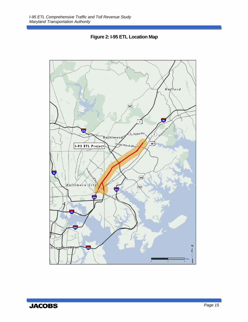
1.4 Project Description The I-95 ETL project extends approximately eight miles. The shortest travel distance on the project is seven miles between MD 43 and Moravia Road; therefore, this distance is used as the tolling distance when calculating toll rates for the facility. The full ETL stretches from north of MD 43 to south of the split of I-95 and I-895, south of Moravia Road and Pulaski Highway, respectively. Figure 2 shows the extent of the ETL.
I-95 ETL Comprehensive Traffic and Toll Revenue Study Maryland Transportation Authority
Page 15
Figure 2: I-95 ETL Location Map
I-95 ETL Comprehensive Traffic and Toll Revenue Study Maryland Transportation Authority
Page 16
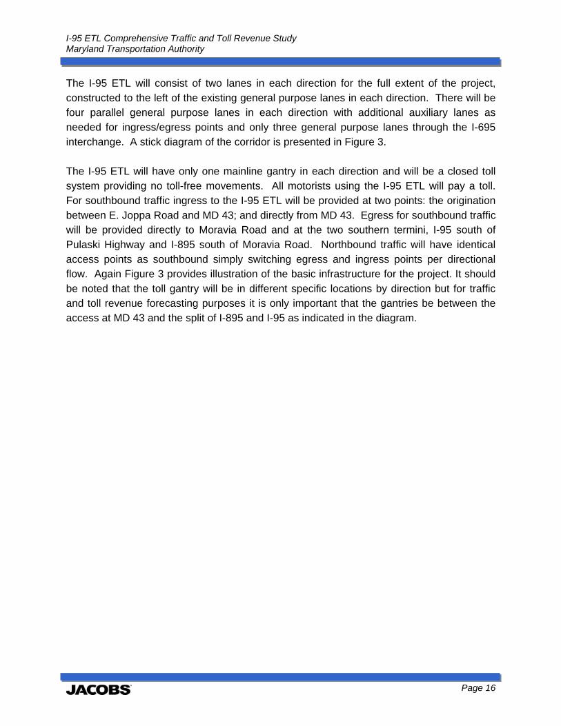
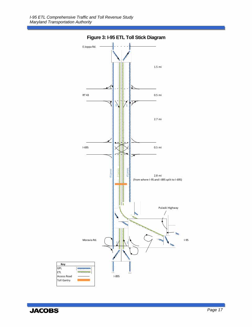
The I-95 ETL will consist of two lanes in each direction for the full extent of the project, constructed to the left of the existing general purpose lanes in each direction. There will be four parallel general purpose lanes in each direction with additional auxiliary lanes as needed for ingress/egress points and only three general purpose lanes through the I-695 interchange. A stick diagram of the corridor is presented in Figure 3. The I-95 ETL will have only one mainline gantry in each direction and will be a closed toll system providing no toll-free movements. All motorists using the I-95 ETL will pay a toll. For southbound traffic ingress to the I-95 ETL will be provided at two points: the origination between E. Joppa Road and MD 43; and directly from MD 43. Egress for southbound traffic will be provided directly to Moravia Road and at the two southern termini, I-95 south of Pulaski Highway and I-895 south of Moravia Road. Northbound traffic will have identical access points as southbound simply switching egress and ingress points per directional flow. Again Figure 3 provides illustration of the basic infrastructure for the project. It should be noted that the toll gantry will be in different specific locations by direction but for traffic and toll revenue forecasting purposes it is only important that the gantries be between the access at MD 43 and the split of I-895 and I-95 as indicated in the diagram.
I-95 ETL Comprehensive Traffic and Toll Revenue Study Maryland Transportation Authority
Page 17
Figure 3: I-95 ETL Toll Stick Diagram
E Joppa Rd.
1.5 mi
RT 43 0.5 mi
2.7 mi
I‐695 0.5 mi
2.8 mi
(from where I‐95 and I‐895 split to I‐695)
Pulaski Highway
Moravia Rd. I‐95
Key
GPL
ETL
Access Road I‐895
Toll Gantry
1 1
1 1
1
1
1 1
11
4 Lanes
4 Lanes
2 Lanes
I-95 ETL Comprehensive Traffic and Toll Revenue Study Maryland Transportation Authority
Page 18
2.0 Tolling Policy Tolling policy for the I-95 ETL is a key driver of traffic and toll revenue estimates for the project. Toll policy leads to the development of a tolling plan that includes toll rate schedules by vehicle and payment classes. MDTA vehicle classes are largely defined by the number of axles. Payment classes reflect the type of payment ranging from cash given to a toll collector at a traditional toll booth to electronically accepted tolls via E-ZPass for a pre-use billing option or video tolling for a post-use billing option. Toll policy also reflects business rules for video tolls, discount programs, special permits and the like. Unlike traditional bridge or expressway fixed toll facilities, the toll policy for tolled managed lanes, such as the I-95 ETL, often has performance standards by which the travel experience in the tolled lanes can be evaluated, leading to changes in the toll rates. To provide a foundation for the proposed toll policy for the I-95 ETL, this section first reviews the tolling policy of the existing MDTA facilities. Then a review of the toll policy of existing managed lane facilities across the United States is undertaken. Finally, the proposed toll policy for the I-95 ETL is presented which reflects a combination of both existing MDTA toll policy and standard managed lane toll policy.
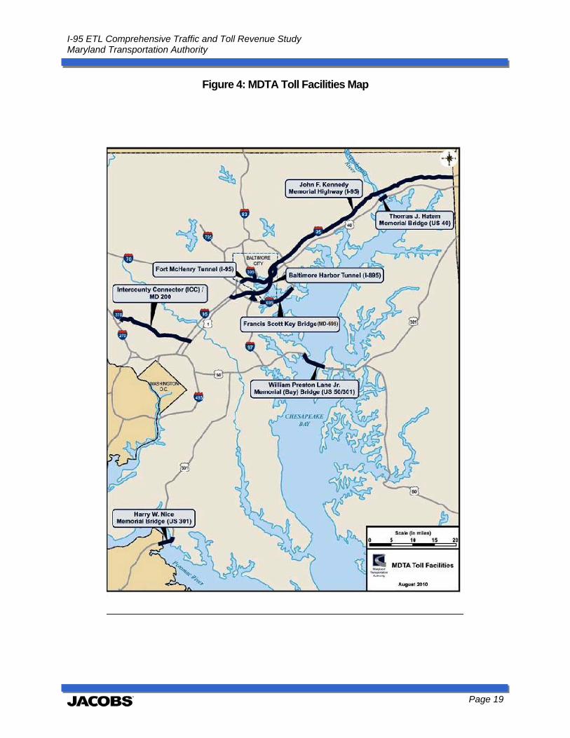
2.1 Existing MDTA Toll Policy As discussed previously, the MDTA currently operates eight toll facilities within the State of Maryland consisting of two expressways, two tunnels and four bridges. For toll policy purposes the seven legacy facilities (excluding the ICC) can be grouped into three categories corresponding to geographic regions of the state: Northern, Central and Southern. These facilities along with the ICC are shown in Figure 4.
I-95 ETL Comprehensive Traffic and Toll Revenue Study Maryland Transportation Authority
Page 19
Figure 4: MDTA Toll Facilities Map

I-95 ETL Comprehensive Traffic and Toll Revenue Study Maryland Transportation Authority
Page 20
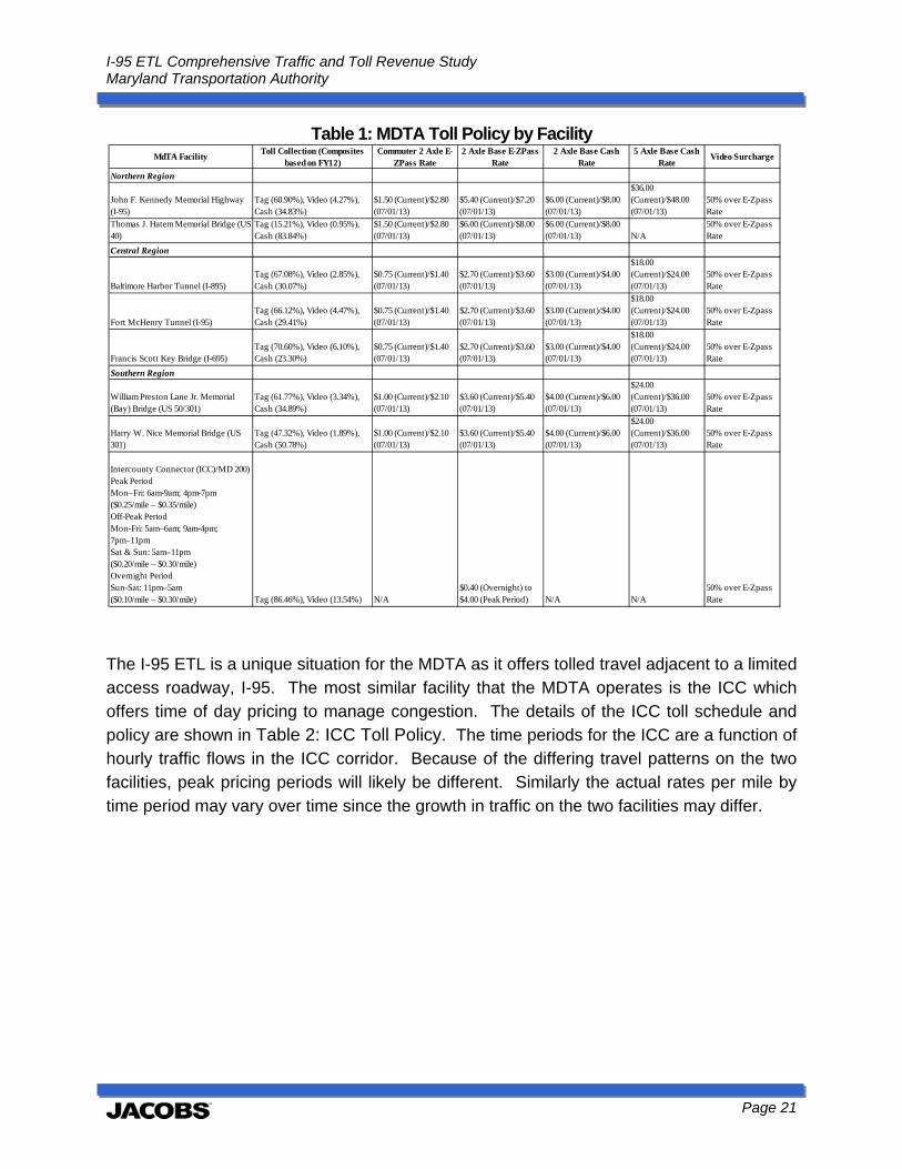
As shown in the figure, all of the seven legacy facilities are on either Interstates or major US routes that cross bodies of water with very limited competing alternatives. In the Northern Region, the John F. Kennedy Memorial Highway (JFK) and Thomas J. Hatem Memorial Bridge (Hatem) provide regional and local connectivity across the Susquehanna River including critical east coast interstate travel connection. In the Central Region, the Fort McHenry Tunnel (FMT), the Baltimore Harbor Tunnel (BHT) and the Francis Scott Key Bridge (FSK) offer access under or over the Baltimore Harbor and are known collectively as the Baltimore Harbor Crossings. In the Southern Region, the William Preston Lane Jr. Memorial (Bay) Bridge, commonly known as the Bay Bridge crosses the Chesapeake Bay providing access between the metropolitan areas to the west and recreational areas on the eastern shore. The Governor Harry W. Nice Memorial Bridge (Nice), also in the Southern Region, provides movement between Maryland and Virginia across the Potomac River. The newest facility in the Southern Region is the Intercounty Connector (ICC/MD 200) which opened in December 2011 and connects I-370 (Gaithersburg) to I-95 (Laurel). With the exception of the ICC (which offers variable pricing to manage congestion), all other MDTA facilities have fixed toll rates that are a function of vehicle and payment classes. Table 1 illustrates some of the toll policy elements for each MDTA facility. There are various programs that are excluded from the table for the sake of simplicity and the goal of comparison.
I-95 ETL Comprehensive Traffic and Toll Revenue Study Maryland Transportation Authority
Page 21
Table 1: MDTA Toll Policy by Facility
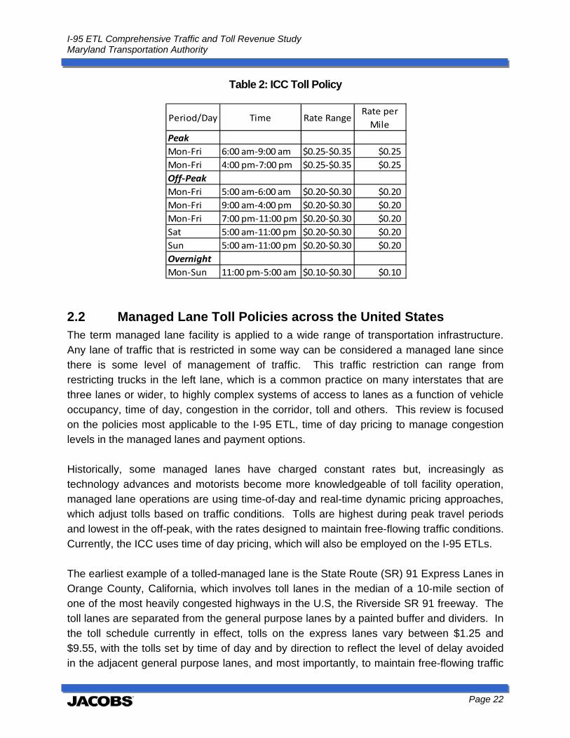
The I-95 ETL is a unique situation for the MDTA as it offers tolled travel adjacent to a limited access roadway, I-95. The most similar facility that the MDTA operates is the ICC which offers time of day pricing to manage congestion. The details of the ICC toll schedule and policy are shown in Table 2: ICC Toll Policy. The time periods for the ICC are a function of hourly traffic flows in the ICC corridor. Because of the differing travel patterns on the two facilities, peak pricing periods will likely be different. Similarly the actual rates per mile by time period may vary over time since the growth in traffic on the two facilities may differ.
MdTA FacilityToll Collection (Composites
based on FY12)Commuter 2 Axle E-
ZPass Rate2 Axle Base E-ZPass
Rate2 Axle Base Cash
Rate5 Axle Base Cash
RateVideo Surcharge
Northern Region
John F. Kennedy Memorial Highway (I-95)
Tag (60.90%), Video (4.27%), Cash (34.83%)
$1.50 (Current)/$2.80 (07/01/13)
$5.40 (Current)/$7.20 (07/01/13)
$6.00 (Current)/$8.00 (07/01/13)
$36.00 (Current)/$48.00 (07/01/13)
50% over E-Zpass Rate
Thomas J. Hatem Memorial Bridge (US 40)
Tag (15.21%), Video (0.95%), Cash (83.84%)
$1.50 (Current)/$2.80 (07/01/13)
$6.00 (Current)/$8.00 (07/01/13)
$6.00 (Current)/$8.00 (07/01/13) N/A
50% over E-Zpass Rate
Central Region
Baltimore Harbor Tunnel (I-895)Tag (67.08%), Video (2.85%), Cash (30.07%)
$0.75 (Current)/$1.40 (07/01/13)
$2.70 (Current)/$3.60 (07/01/13)
$3.00 (Current)/$4.00 (07/01/13)
$18.00 (Current)/$24.00 (07/01/13)
50% over E-Zpass Rate
Fort McHenry Tunnel (I-95)Tag (66.12%), Video (4.47%), Cash (29.41%)
$0.75 (Current)/$1.40 (07/01/13)
$2.70 (Current)/$3.60 (07/01/13)
$3.00 (Current)/$4.00 (07/01/13)
$18.00 (Current)/$24.00 (07/01/13)
50% over E-Zpass Rate
Francis Scott Key Bridge (I-695)Tag (70.60%), Video (6.10%), Cash (23.30%)
$0.75 (Current)/$1.40 (07/01/13)
$2.70 (Current)/$3.60 (07/01/13)
$3.00 (Current)/$4.00 (07/01/13)
$18.00 (Current)/$24.00 (07/01/13)
50% over E-Zpass Rate
Southern Region
William Preston Lane Jr. Memorial (Bay) Bridge (US 50/301)
Tag (61.77%), Video (3.34%), Cash (34.89%)
$1.00 (Current)/$2.10 (07/01/13)
$3.60 (Current)/$5.40 (07/01/13)
$4.00 (Current)/$6.00 (07/01/13)
$24.00 (Current)/$36.00 (07/01/13)
50% over E-Zpass Rate
Harry W. Nice Memorial Bridge (US 301)
Tag (47.32%), Video (1.89%), Cash (50.78%)
$1.00 (Current)/$2.10 (07/01/13)
$3.60 (Current)/$5.40 (07/01/13)
$4.00 (Current)/$6.00 (07/01/13)
$24.00 (Current)/$36.00 (07/01/13)
50% over E-Zpass Rate
Intercounty Connector (ICC)/MD 200)Peak PeriodMon–Fri: 6am-9am; 4pm-7pm($0.25/mile – $0.35/mile)Off-Peak PeriodMon-Fri: 5am–6am; 9am-4pm; 7pm–11pmSat & Sun: 5am–11pm($0.20/mile – $0.30/mile)Overnight PeriodSun-Sat: 11pm–5am($0.10/mile – $0.30/mile) Tag (86.46%), Video (13.54%) N/A
$0.40 (Overnight) to $4.00 (Peak Period) N/A N/A
50% over E-Zpass Rate
I-95 ETL Comprehensive Traffic and Toll Revenue Study Maryland Transportation Authority
Page 22
Table 2: ICC Toll Policy
2.2 Managed Lane Toll Policies across the United States The term managed lane facility is applied to a wide range of transportation infrastructure. Any lane of traffic that is restricted in some way can be considered a managed lane since there is some level of management of traffic. This traffic restriction can range from restricting trucks in the left lane, which is a common practice on many interstates that are three lanes or wider, to highly complex systems of access to lanes as a function of vehicle occupancy, time of day, congestion in the corridor, toll and others. This review is focused on the policies most applicable to the I-95 ETL, time of day pricing to manage congestion levels in the managed lanes and payment options. Historically, some managed lanes have charged constant rates but, increasingly as technology advances and motorists become more knowledgeable of toll facility operation, managed lane operations are using time-of-day and real-time dynamic pricing approaches, which adjust tolls based on traffic conditions. Tolls are highest during peak travel periods and lowest in the off-peak, with the rates designed to maintain free-flowing traffic conditions. Currently, the ICC uses time of day pricing, which will also be employed on the I-95 ETLs. The earliest example of a tolled-managed lane is the State Route (SR) 91 Express Lanes in Orange County, California, which involves toll lanes in the median of a 10-mile section of one of the most heavily congested highways in the U.S, the Riverside SR 91 freeway. The toll lanes are separated from the general purpose lanes by a painted buffer and dividers. In the toll schedule currently in effect, tolls on the express lanes vary between $1.25 and $9.55, with the tolls set by time of day and by direction to reflect the level of delay avoided in the adjacent general purpose lanes, and most importantly, to maintain free-flowing traffic
Period/Day Time Rate RangeRate per
Mile
Peak
Mon‐Fri 6:00 am‐9:00 am $0.25‐$0.35 $0.25
Mon‐Fri 4:00 pm‐7:00 pm $0.25‐$0.35 $0.25
Off‐Peak
Mon‐Fri 5:00 am‐6:00 am $0.20‐$0.30 $0.20
Mon‐Fri 9:00 am‐4:00 pm $0.20‐$0.30 $0.20
Mon‐Fri 7:00 pm‐11:00 pm $0.20‐$0.30 $0.20
Sat 5:00 am‐11:00 pm $0.20‐$0.30 $0.20
Sun 5:00 am‐11:00 pm $0.20‐$0.30 $0.20
Overnight
Mon‐Sun 11:00 pm‐5:00 am $0.10‐$0.30 $0.10
I-95 ETL Comprehensive Traffic and Toll Revenue Study Maryland Transportation Authority
Page 23
conditions in the toll lanes. Toll rates can be increased as often as every six (6) months. The $9.55 toll during the “super peak” represents $0.96 per mile, the highest toll rate for any toll road in the country. Under this toll schedule, revenues have been adequate to pay for construction and operating costs. Currently, the I-15 Express Lanes in San Diego are being extended to create a 20-mile "Managed Lanes" facility in the median of I-15 between SR 163 and SR 78. When complete, there will be a four-lane facility in the median with a moveable barrier, multiple access points from the regular highway lanes, and direct access ramps for buses from five (5) transit centers. A high frequency bus rapid transit (BRT) system is under development and will replace the existing express buses that serve the corridor. The technological capability to vary the price for the use of these facilities throughout the day has given transportation agencies a powerful tool for maintaining a certain level of service in the managed lanes. While there have been concerns about equity impacts, research on the demographic and economic profile the customers on the 91 Express Lanes has shown that “…users from all income groups regularly make use of the facility.” More recent experience confirms this usage pattern; in the Seattle area, it was noted of the SR 167 managed lanes that “they are more like "Ford Lanes," reflecting the most common make of vehicle that used the lanes from May through July of 2008. Drivers view the managed lanes as a choice when the value of time savings outweighs the cost of using the facility, in effect as a form of congestion insurance. Figure 5 illustrates all operating tolled managed lane facilities in the United States.

I-95 ETL Comprehensive Traffic and Toll Revenue Study Maryland Transportation Authority
Page 24
Figure 5: Toll Policy on Existing U.S. Managed Lane Facilities
I-95 ETL Comprehensive Traffic and Toll Revenue Study Maryland Transportation Authority
Page 25
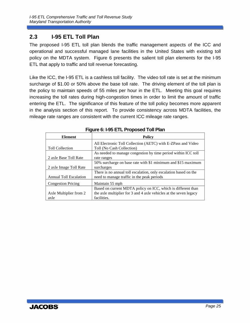
2.3 I-95 ETL Toll Plan The proposed I-95 ETL toll plan blends the traffic management aspects of the ICC and operational and successful managed lane facilities in the United States with existing toll policy on the MDTA system. Figure 6 presents the salient toll plan elements for the I-95 ETL that apply to traffic and toll revenue forecasting. Like the ICC, the I-95 ETL is a cashless toll facility. The video toll rate is set at the minimum surcharge of $1.00 or 50% above the base toll rate. The driving element of the toll plan is the policy to maintain speeds of 55 miles per hour in the ETL. Meeting this goal requires increasing the toll rates during high-congestion times in order to limit the amount of traffic entering the ETL. The significance of this feature of the toll policy becomes more apparent in the analysis section of this report. To provide consistency across MDTA facilities, the mileage rate ranges are consistent with the current ICC mileage rate ranges.
Figure 6: I-95 ETL Proposed Toll Plan
Element Policy
Toll Collection All Electronic Toll Collection (AETC) with E-ZPass and Video Toll (No Cash Collection)
2 axle Base Toll Rate As needed to manage congestion by time period within ICC toll rate ranges
2 axle Image Toll Rate 50% surcharge on base rate with $1 minimum and $15 maximum surcharges
Annual Toll Escalation There is no annual toll escalation, only escalation based on the need to manage traffic in the peak periods
Congestion Pricing Maintain 55 mph
Axle Multiplier from 2 axle
Based on current MDTA policy on ICC, which is different than the axle multiplier for 3 and 4 axle vehicles at the seven legacy facilities.
I-95 ETL Comprehensive Traffic and Toll Revenue Study Maryland Transportation Authority
Page 26
3.0 Corridor Traffic Conditions Existing traffic conditions provide an empirical snapshot of how traffic functions today. This combined with the historical experience in the corridor, year over year, and forecasted traffic volumes provide key inputs to the traffic and toll revenue forecasting model. The I-95 ETL extend approximately eight miles, between the I-95/I-895 split from the Baltimore city line (mile marker 62) to just north of MD 43/Whitemarsh Boulevard (mile marker 70).
3.1 Historical Traffic Conditions Table 3 presents average annual traffic counts from 1980 through 2011for the portion of I-95 to be served by the ETL. From 1980 to 1990, traffic along the project corridor grew at an average annual rate of 9.7% and from 1990 to 2000 at an annual rate of 1.0%. Over the last decade, traffic increased at an annual rate of 0.9% within the segments just south of the I-695 interchange and north of MD 43/Whitemarsh Boulevard growing at an annual rate of 1.1% and 1.3%, respectively. For the 2011 calendar year, average daily traffic volumes in the mid-section of the corridor ranged from 160,100 north of the I-695 interchange to 165,300 south of the I-695 interchange. Average daily traffic volumes for the southern termini locations ranged from 58,500 on I-895 north of US 40/Pulaski Hwy to 97,300 on I-95 north of US 40/Pulaski Hwy. The northern terminius north of MD 43/Whitemarsh Boulevard experienced average daily traffic of 161,700.

I-95 ETL Comprehensive Traffic and Toll Revenue Study Maryland Transportation Authority
Page 27
Table 3: Historical Traffic Volumes (1980-2011)
Year
Average Annual Daily Traffic Trends
I-895 N of
Pulaski Hwy
I-95 N of
Pulaski Hwy
S of I-95/I-695
Interchange
N of I-95/I-695
Interchange
I-95 N of MD 43/Whitemarsh
Blvd
1980 9,985 16,050 65,685 62,250 56,700
1990 46,550 74,830 133,950 155,020 119,500
2000 55,950 89,950 161,000 141,175 139,575
2001 57,125 91,875 147,537 150,150 142,450
2002 58,375 98,375 134,075 151,725 143,925
2003 58,450 98,450 151,175 157,675 171,975
2004 59,025 99,425 152,750 159,350 173,750
2005 59,975 98,875 161,775 159,425 173,825
2006 59,981 98,881 168,020 162,770 161,780
2007 59,982 98,882 168,021 162,771 161,781
2008 57,660 95,823 162,812 157,722 157,742
2009 58,241 96,784 164,443 159,303 160,880
2010 58,472 97,175 165,104 159,943 161,521
2011 58,480 97,275 165,275 160,109 161,682
Average Annual Percent Change 2001-2006 1.00% 1.53% 2.78% 1.68% 2.71%
2006-2011 -0.50% -0.32% -0.33% -0.33% -0.01%
2001-2011 0.24% 0.59% 1.20% 0.66% 1.35%
Source: Maryland State Highway Administration Traffic Volume Maps
3.2 Existing Traffic Conditions In 2011, average daily traffic volumes in the I-95 ETL project corridor ranged from approximately 160,000 vehicles per day north of I-695 to 165,000 vehicles per day south of I-695. The section south of the I-95/I-895 split experienced average daily traffic volumes of approximately 97,000 vehicles per day on I-95 and approximately 58,000 vehicles per day on I-895. In this section, the annual average daily traffic volumes for the corridor are detailed by day of the week and hour as is the relationship between volume and speed. This detailed breakdown of traffic volume and the relationship to speed is critical to this analysis because time savings is the driver of motorists’ behavior when choosing a tolled alternative.
I-95 ETL Comprehensive Traffic and Toll Revenue Study Maryland Transportation Authority
Page 28
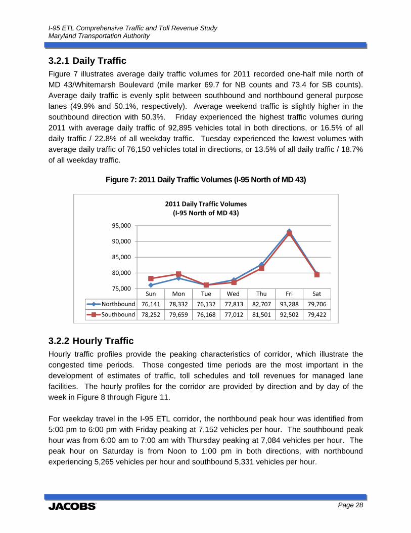
3.2.1 Daily Traffic Figure 7 illustrates average daily traffic volumes for 2011 recorded one-half mile north of MD 43/Whitemarsh Boulevard (mile marker 69.7 for NB counts and 73.4 for SB counts). Average daily traffic is evenly split between southbound and northbound general purpose lanes (49.9% and 50.1%, respectively). Average weekend traffic is slightly higher in the southbound direction with 50.3%. Friday experienced the highest traffic volumes during 2011 with average daily traffic of 92,895 vehicles total in both directions, or 16.5% of all daily traffic / 22.8% of all weekday traffic. Tuesday experienced the lowest volumes with average daily traffic of 76,150 vehicles total in directions, or 13.5% of all daily traffic / 18.7% of all weekday traffic.
Figure 7: 2011 Daily Traffic Volumes (I-95 North of MD 43)
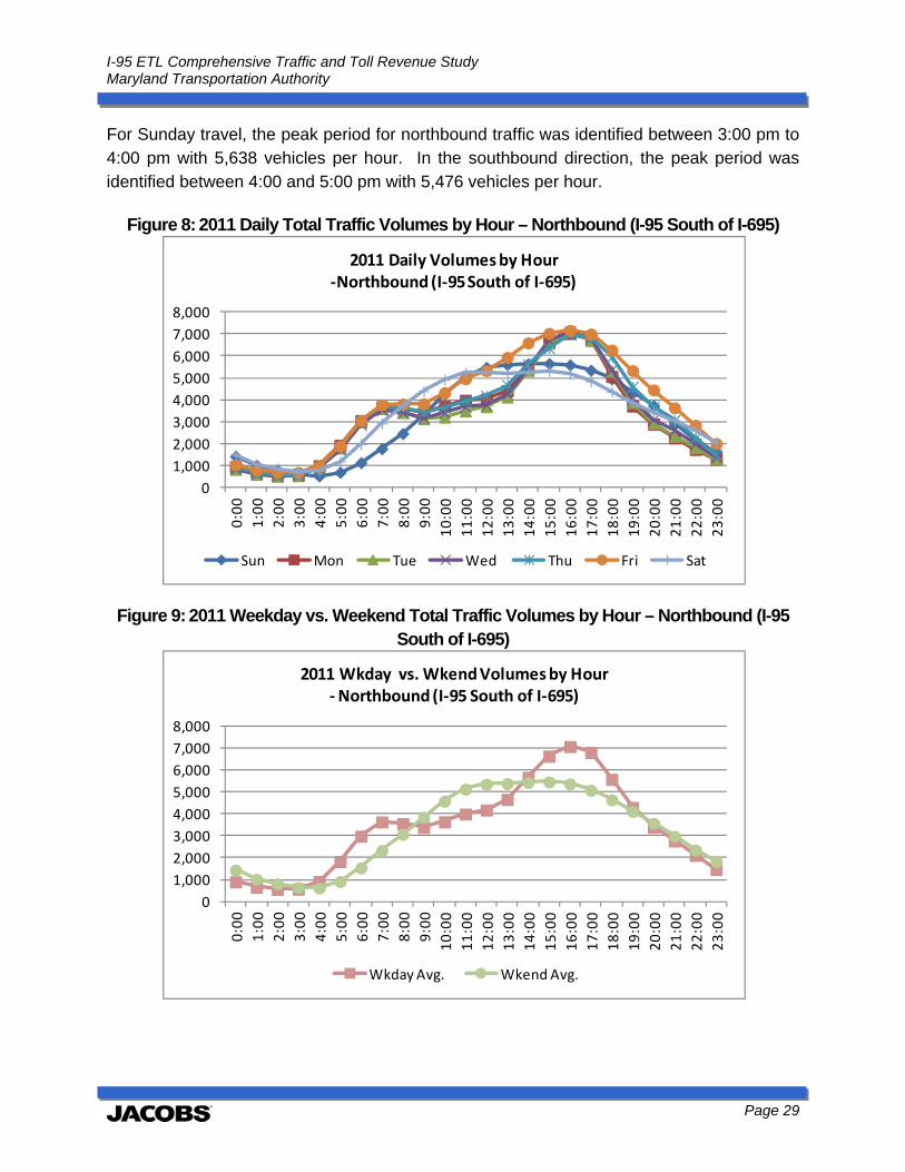
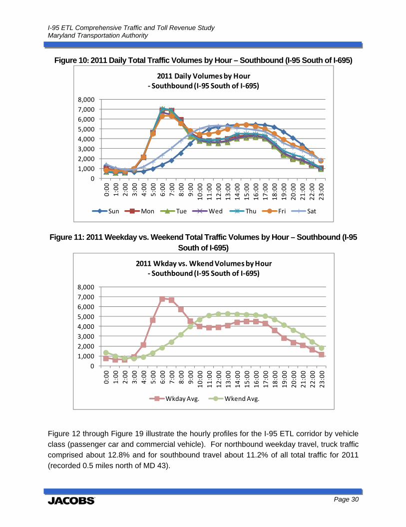
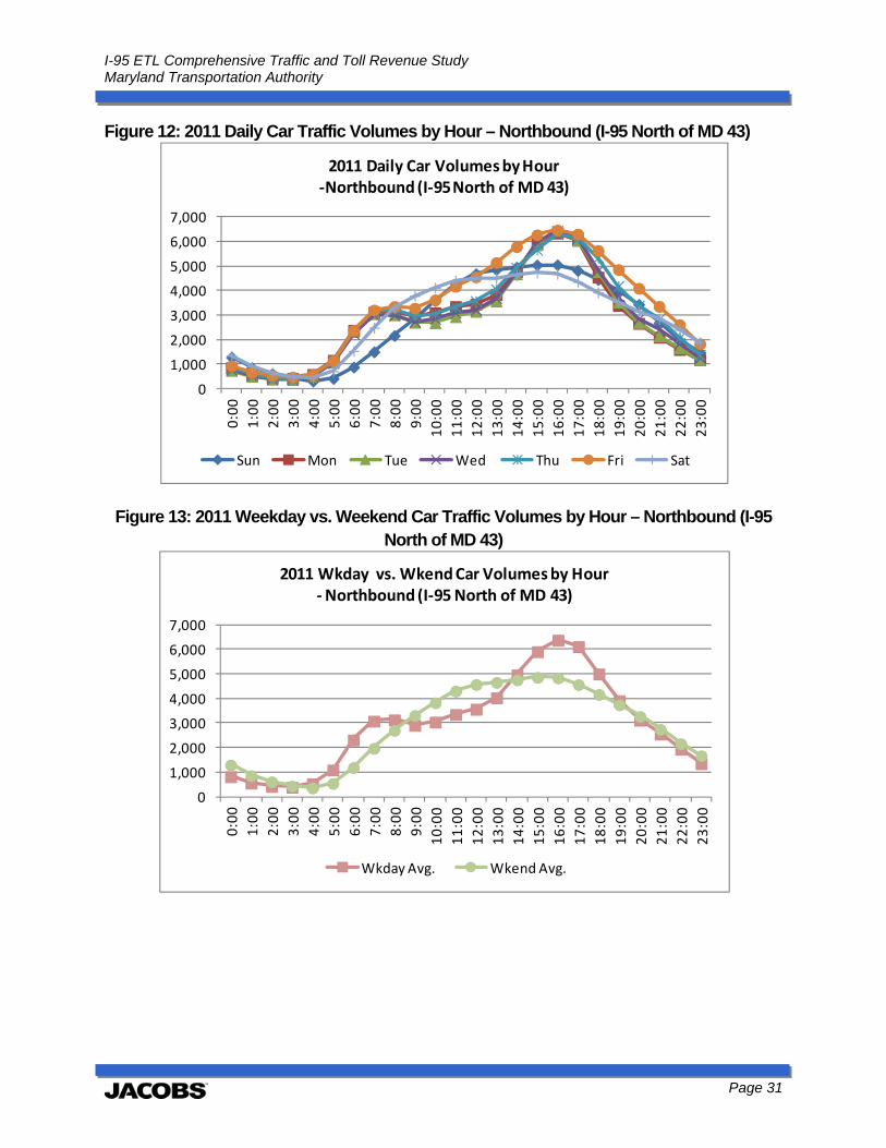
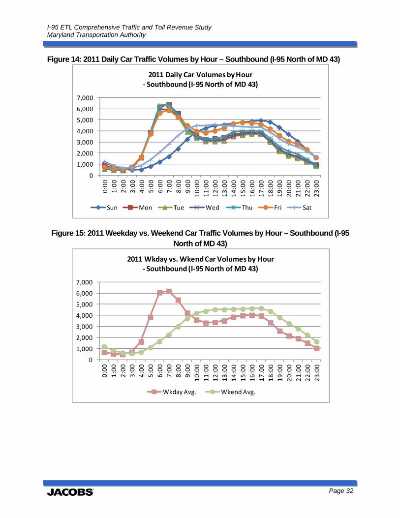
3.2.2 Hourly Traffic Hourly traffic profiles provide the peaking characteristics of corridor, which illustrate the congested time periods. Those congested time periods are the most important in the development of estimates of traffic, toll schedules and toll revenues for managed lane facilities. The hourly profiles for the corridor are provided by direction and by day of the week in Figure 8 through Figure 11. For weekday travel in the I-95 ETL corridor, the northbound peak hour was identified from 5:00 pm to 6:00 pm with Friday peaking at 7,152 vehicles per hour. The southbound peak hour was from 6:00 am to 7:00 am with Thursday peaking at 7,084 vehicles per hour. The peak hour on Saturday is from Noon to 1:00 pm in both directions, with northbound experiencing 5,265 vehicles per hour and southbound 5,331 vehicles per hour.
Sun Mon Tue Wed Thu Fri Sat
Northbound 76,141 78,332 76,132 77,813 82,707 93,288 79,706
Southbound 78,252 79,659 76,168 77,012 81,501 92,502 79,422
75,000
80,000
85,000
90,000
95,000
2011 Daily Traffic Volumes (I‐95 North of MD 43)
I-95 ETL Comprehensive Traffic and Toll Revenue Study Maryland Transportation Authority
Page 29
For Sunday travel, the peak period for northbound traffic was identified between 3:00 pm to 4:00 pm with 5,638 vehicles per hour. In the southbound direction, the peak period was identified between 4:00 and 5:00 pm with 5,476 vehicles per hour.
Figure 8: 2011 Daily Total Traffic Volumes by Hour – Northbound (I-95 South of I-695)
Figure 9: 2011 Weekday vs. Weekend Total Traffic Volumes by Hour – Northbound (I-95 South of I-695)
0
1,000
2,000
3,000
4,000
5,000
6,000
7,000
8,000
0:00
1:00
2:00
3:00
4:00
5:00
6:00
7:00
8:00
9:00
10:00
11:00
12:00
13:00
14:00
15:00
16:00
17:00
18:00
19:00
20:00
21:00
22:00
23:00
2011 Daily Volumes by Hour ‐Northbound (I‐95 South of I‐695)
Sun Mon Tue Wed Thu Fri Sat
0
1,000
2,000
3,000
4,000
5,000
6,000
7,000
8,000
0:00
1:00
2:00
3:00
4:00
5:00
6:00
7:00
8:00
9:00
10:00
11:00
12:00
13:00
14:00
15:00
16:00
17:00
18:00
19:00
20:00
21:00
22:00
23:00
2011 Wkday vs. Wkend Volumes by Hour ‐Northbound (I‐95 South of I‐695)
Wkday Avg. Wkend Avg.
I-95 ETL Comprehensive Traffic and Toll Revenue Study Maryland Transportation Authority
Page 30
Figure 10: 2011 Daily Total Traffic Volumes by Hour – Southbound (I-95 South of I-695)
Figure 11: 2011 Weekday vs. Weekend Total Traffic Volumes by Hour – Southbound (I-95 South of I-695)
Figure 12 through Figure 19 illustrate the hourly profiles for the I-95 ETL corridor by vehicle class (passenger car and commercial vehicle). For northbound weekday travel, truck traffic comprised about 12.8% and for southbound travel about 11.2% of all total traffic for 2011 (recorded 0.5 miles north of MD 43).
0
1,000
2,000
3,000
4,000
5,000
6,000
7,000
8,0000:00
1:00
2:00
3:00
4:00
5:00
6:00
7:00
8:00
9:00
10:00
11:00
12:00
13:00
14:00
15:00
16:00
17:00
18:00
19:00
20:00
21:00
22:00
23:00
2011 Daily Volumes by Hour‐ Southbound (I‐95 South of I‐695)
Sun Mon Tue Wed Thu Fri Sat
0
1,000
2,000
3,000
4,000
5,000
6,000
7,000
8,000
0:00
1:00
2:00
3:00
4:00
5:00
6:00
7:00
8:00
9:00
10:00
11:00
12:00
13:00
14:00
15:00
16:00
17:00
18:00
19:00
20:00
21:00
22:00
23:00
2011 Wkday vs. Wkend Volumes by Hour ‐ Southbound (I‐95 South of I‐695)
Wkday Avg. Wkend Avg.
I-95 ETL Comprehensive Traffic and Toll Revenue Study Maryland Transportation Authority
Page 31
Figure 12: 2011 Daily Car Traffic Volumes by Hour – Northbound (I-95 North of MD 43)
Figure 13: 2011 Weekday vs. Weekend Car Traffic Volumes by Hour – Northbound (I-95 North of MD 43)
0
1,000
2,000
3,000
4,000
5,000
6,000
7,0000:00
1:00
2:00
3:00
4:00
5:00
6:00
7:00
8:00
9:00
10:00
11:00
12:00
13:00
14:00
15:00
16:00
17:00
18:00
19:00
20:00
21:00
22:00
23:00
2011 Daily Car Volumes by Hour ‐Northbound (I‐95 North of MD 43)
Sun Mon Tue Wed Thu Fri Sat
0
1,000
2,000
3,000
4,000
5,000
6,000
7,000
0:00
1:00
2:00
3:00
4:00
5:00
6:00
7:00
8:00
9:00
10:00
11:00
12:00
13:00
14:00
15:00
16:00
17:00
18:00
19:00
20:00
21:00
22:00
23:00
2011 Wkday vs. Wkend Car Volumes by Hour ‐Northbound (I‐95 North of MD 43)
Wkday Avg. Wkend Avg.
I-95 ETL Comprehensive Traffic and Toll Revenue Study Maryland Transportation Authority
Page 32
Figure 14: 2011 Daily Car Traffic Volumes by Hour – Southbound (I-95 North of MD 43)
Figure 15: 2011 Weekday vs. Weekend Car Traffic Volumes by Hour – Southbound (I-95 North of MD 43)
0
1,000
2,000
3,000
4,000
5,000
6,000
7,0000:00
1:00
2:00
3:00
4:00
5:00
6:00
7:00
8:00
9:00
10:00
11:00
12:00
13:00
14:00
15:00
16:00
17:00
18:00
19:00
20:00
21:00
22:00
23:00
2011 Daily Car Volumes by Hour‐ Southbound (I‐95 North of MD 43)
Sun Mon Tue Wed Thu Fri Sat
0
1,000
2,000
3,000
4,000
5,000
6,000
7,000
0:00
1:00
2:00
3:00
4:00
5:00
6:00
7:00
8:00
9:00
10:00
11:00
12:00
13:00
14:00
15:00
16:00
17:00
18:00
19:00
20:00
21:00
22:00
23:00
2011 Wkday vs. Wkend Car Volumes by Hour ‐ Southbound (I‐95 North of MD 43)
Wkday Avg. Wkend Avg.
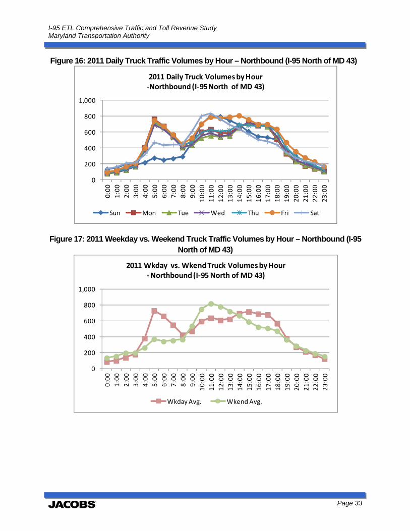
I-95 ETL Comprehensive Traffic and Toll Revenue Study Maryland Transportation Authority
Page 33
Figure 16: 2011 Daily Truck Traffic Volumes by Hour – Northbound (I-95 North of MD 43)
Figure 17: 2011 Weekday vs. Weekend Truck Traffic Volumes by Hour – Northbound (I-95 North of MD 43)
0
200
400
600
800
1,0000:00
1:00
2:00
3:00
4:00
5:00
6:00
7:00
8:00
9:00
10:00
11:00
12:00
13:00
14:00
15:00
16:00
17:00
18:00
19:00
20:00
21:00
22:00
23:00
2011 Daily Truck Volumes by Hour ‐Northbound (I‐95 North of MD 43)
Sun Mon Tue Wed Thu Fri Sat
0
200
400
600
800
1,000
0:00
1:00
2:00
3:00
4:00
5:00
6:00
7:00
8:00
9:00
10:00
11:00
12:00
13:00
14:00
15:00
16:00
17:00
18:00
19:00
20:00
21:00
22:00
23:00
2011 Wkday vs. Wkend Truck Volumes by Hour ‐Northbound (I‐95 North of MD 43)
Wkday Avg. Wkend Avg.
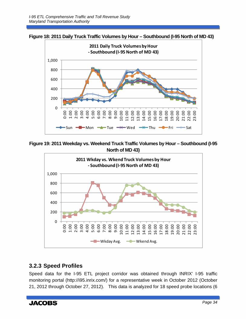
I-95 ETL Comprehensive Traffic and Toll Revenue Study Maryland Transportation Authority
Page 34
Figure 18: 2011 Daily Truck Traffic Volumes by Hour – Southbound (I-95 North of MD 43)
Figure 19: 2011 Weekday vs. Weekend Truck Traffic Volumes by Hour – Southbound (I-95 North of MD 43)
3.2.3 Speed Profiles Speed data for the I-95 ETL project corridor was obtained through INRIX’ I-95 traffic monitoring portal (http://i95.inrix.com/) for a representative week in October 2012 (October 21, 2012 through October 27, 2012). This data is analyzed for 18 speed probe locations (6
0
200
400
600
800
1,0000:00
1:00
2:00
3:00
4:00
5:00
6:00
7:00
8:00
9:00
10:00
11:00
12:00
13:00
14:00
15:00
16:00
17:00
18:00
19:00
20:00
21:00
22:00
23:00
2011 Daily Truck Volumes by Hour‐ Southbound (I‐95 North of MD 43)
Sun Mon Tue Wed Thu Fri Sat
0
200
400
600
800
1,000
0:00
1:00
2:00
3:00
4:00
5:00
6:00
7:00
8:00
9:00
10:00
11:00
12:00
13:00
14:00
15:00
16:00
17:00
18:00
19:00
20:00
21:00
22:00
23:00
2011 Wkday vs. Wkend Truck Volumes by Hour ‐ Southbound (I‐95 North of MD 43)
Wkday Avg. Wkend Avg.

I-95 ETL Comprehensive Traffic and Toll Revenue Study Maryland Transportation Authority
Page 35
along I-95 and 3 along I-895 in each direction). Speed profiles for the 6:00 am to 9:00 am southbound morning peak period and 4:00 pm to 7:00 pm northbound afternoon peak period as well as the 7:00 am to 8:00 am southbound morning peak hour and 5:00 pm to 6:00 pm northbound afternoon peak hour are summarized in Figure 20 through Figure 23. Average weekday speeds on I-95 during the southbound morning peak period are calculated at 52.9 mph and northbound afternoon speeds at 49.8 mph. During the peak morning and afternoon hours, speeds drop significantly with average southbound speeds during the 7:00 am to 8:00 am southbound morning peak hour calculated at 43 mph and during the northbound afternoon peak hour at 37.3 mph. This represents a 19% drop in morning southbound and 25% drop in afternoon northbound speeds between periods and hour, respectively. Overall, average weekday southbound speeds along the I-95 ETL corridor are 62.3 mph and average weekday northbound speeds at 59.8 mph. Average weekend speeds were slightly higher at 65.6 mph southbound and 63.9 mph northbound.
Figure 20: I-95/I-895 Average Southbound Speeds During Morning Peak Period
1015202530354045505560657075
Sun Mon Tue Wed Thu Fri Sat
I‐95/I‐895 Average Southbound Speeds During 6:00 am‐9:00 am Peak Period
I‐95 @ MD‐43/WhitemarshBlvd/Exit 67 (110N04442) ‐ SBI‐95 @ I‐695/Exit 64 (110‐04441) ‐SBI‐95 @ I‐695/Exit 64 (110N04441) ‐SBI‐95 @ I‐895/62nd St/Exit 62 (110‐04440) ‐ SBI‐95 @ I‐895/62nd St/Exit 62(110N04440) ‐ SBI‐95 @ US‐40/Pulaski Hwy/Exit 61(110‐04439) ‐ SBI‐895 @ Moravia Rd/Exit 14 (110‐04578) ‐ SBI‐895 @ Moravia Rd/Exit 14(110N04578) ‐ SB
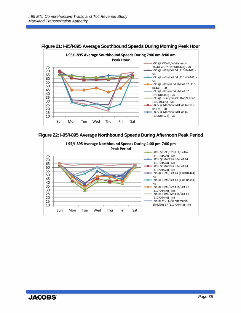
I-95 ETL Comprehensive Traffic and Toll Revenue Study Maryland Transportation Authority
Page 36
Figure 21: I-95/I-895 Average Southbound Speeds During Morning Peak Hour
Figure 22: I-95/I-895 Average Northbound Speeds During Afternoon Peak Period
1015202530354045505560657075
Sun Mon Tue Wed Thu Fri Sat
I‐95/I‐895 Average Southbound Speeds During 7:00 am‐8:00 am Peak Hour
I‐95 @ MD‐43/WhitemarshBlvd/Exit 67 (110N04442) ‐ SBI‐95 @ I‐695/Exit 64 (110‐04441) ‐SBI‐95 @ I‐695/Exit 64 (110N04441) ‐SBI‐95 @ I‐895/62nd St/Exit 62 (110‐04440) ‐ SBI‐95 @ I‐895/62nd St/Exit 62(110N04440) ‐ SBI‐95 @ US‐40/Pulaski Hwy/Exit 61(110‐04439) ‐ SBI‐895 @ Moravia Rd/Exit 14 (110‐04578) ‐ SBI‐895 @ Moravia Rd/Exit 14(110N04578) ‐ SB
1015202530354045505560657075
Sun Mon Tue Wed Thu Fri Sat
I‐95/I‐895 Average Northbound Speeds During 4:00 pm‐7:00 pm Peak Period
I‐895 @ I‐95/62nd St/Exit62(110+04579) ‐ NBI‐895 @ Moravia Rd/Exit 14(110+04578) ‐ NBI‐895 @ Moravia Rd/Exit 14(110P04578) ‐ NBI‐95 @ I‐695/Exit 64 (110+04441) ‐NBI‐95 @ I‐695/Exit 64 (110P04441) ‐NBI‐95 @ I‐895/62nd St/Exit 62(110+04440) ‐ NBI‐95 @ I‐895/62nd St/Exit 62(110P04440) ‐ NBI‐95 @ MD‐43/WhitemarshBlvd/Exit 67 (110+04442) ‐ NB
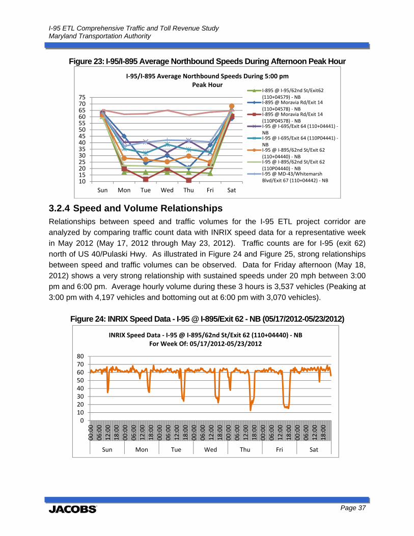
I-95 ETL Comprehensive Traffic and Toll Revenue Study Maryland Transportation Authority
Page 37
Figure 23: I-95/I-895 Average Northbound Speeds During Afternoon Peak Hour
3.2.4 Speed and Volume Relationships Relationships between speed and traffic volumes for the I-95 ETL project corridor are analyzed by comparing traffic count data with INRIX speed data for a representative week in May 2012 (May 17, 2012 through May 23, 2012). Traffic counts are for I-95 (exit 62) north of US 40/Pulaski Hwy. As illustrated in Figure 24 and Figure 25, strong relationships between speed and traffic volumes can be observed. Data for Friday afternoon (May 18, 2012) shows a very strong relationship with sustained speeds under 20 mph between 3:00 pm and 6:00 pm. Average hourly volume during these 3 hours is 3,537 vehicles (Peaking at 3:00 pm with 4,197 vehicles and bottoming out at 6:00 pm with 3,070 vehicles).
Figure 24: INRIX Speed Data - I-95 @ I-895/Exit 62 - NB (05/17/2012-05/23/2012)
1015202530354045505560657075
Sun Mon Tue Wed Thu Fri Sat
I‐95/I‐895 Average Northbound Speeds During 5:00 pm Peak Hour
I‐895 @ I‐95/62nd St/Exit62(110+04579) ‐ NBI‐895 @ Moravia Rd/Exit 14(110+04578) ‐ NBI‐895 @ Moravia Rd/Exit 14(110P04578) ‐ NBI‐95 @ I‐695/Exit 64 (110+04441) ‐NBI‐95 @ I‐695/Exit 64 (110P04441) ‐NBI‐95 @ I‐895/62nd St/Exit 62(110+04440) ‐ NBI‐95 @ I‐895/62nd St/Exit 62(110P04440) ‐ NBI‐95 @ MD‐43/WhitemarshBlvd/Exit 67 (110+04442) ‐ NB
01020304050607080
00:00
06:00
12:00
18:00
00:00
06:00
12:00
18:00
00:00
06:00
12:00
18:00
00:00
06:00
12:00
18:00
00:00
06:00
12:00
18:00
00:00
06:00
12:00
18:00
00:00
06:00
12:00
18:00
Sun Mon Tue Wed Thu Fri Sat
INRIX Speed Data ‐ I‐95 @ I‐895/62nd St/Exit 62 (110+04440) ‐ NBFor Week Of: 05/17/2012‐05/23/2012
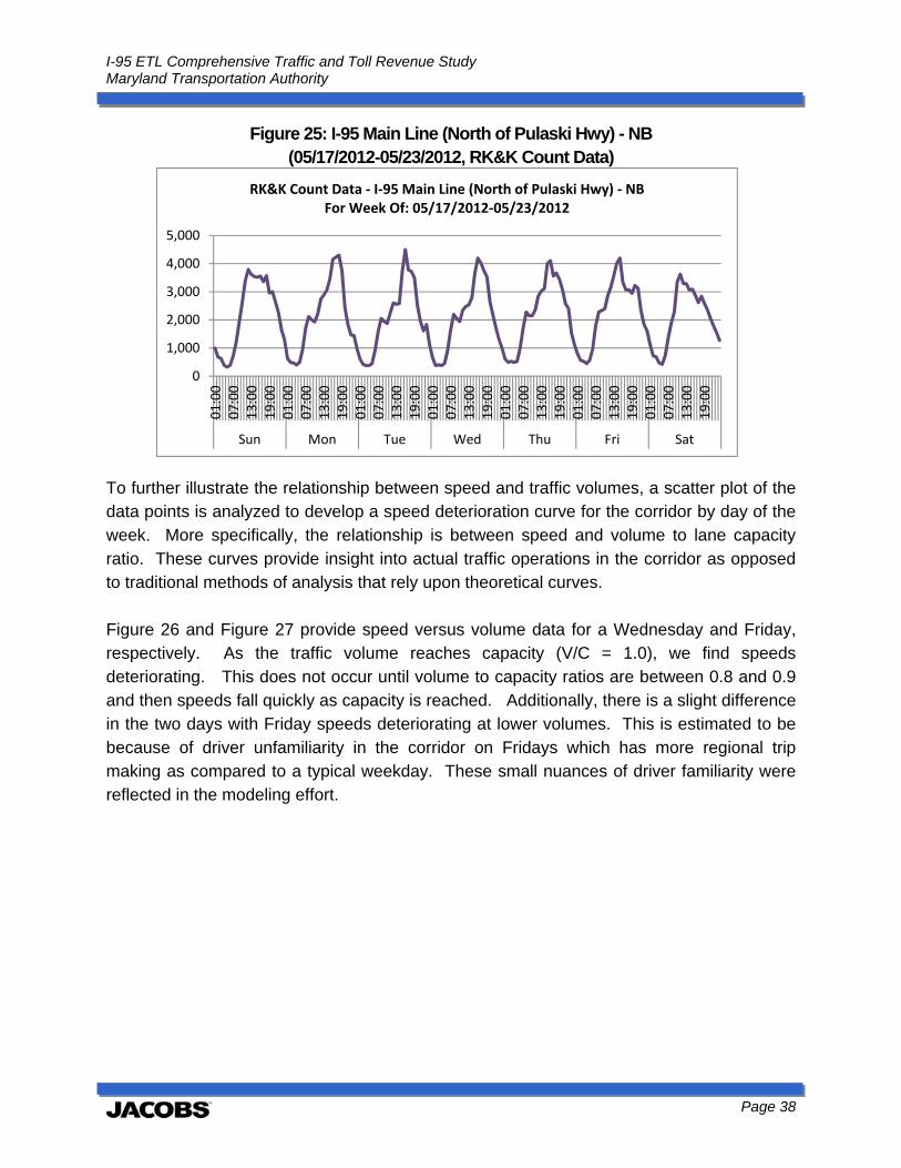
I-95 ETL Comprehensive Traffic and Toll Revenue Study Maryland Transportation Authority
Page 38
Figure 25: I-95 Main Line (North of Pulaski Hwy) - NB (05/17/2012-05/23/2012, RK&K Count Data)
To further illustrate the relationship between speed and traffic volumes, a scatter plot of the data points is analyzed to develop a speed deterioration curve for the corridor by day of the week. More specifically, the relationship is between speed and volume to lane capacity ratio. These curves provide insight into actual traffic operations in the corridor as opposed to traditional methods of analysis that rely upon theoretical curves. Figure 26 and Figure 27 provide speed versus volume data for a Wednesday and Friday, respectively. As the traffic volume reaches capacity (V/C = 1.0), we find speeds deteriorating. This does not occur until volume to capacity ratios are between 0.8 and 0.9 and then speeds fall quickly as capacity is reached. Additionally, there is a slight difference in the two days with Friday speeds deteriorating at lower volumes. This is estimated to be because of driver unfamiliarity in the corridor on Fridays which has more regional trip making as compared to a typical weekday. These small nuances of driver familiarity were reflected in the modeling effort.
0
1,000
2,000
3,000
4,000
5,000
01:00
07:00
13:00
19:00
01:00
07:00
13:00
19:00
01:00
07:00
13:00
19:00
01:00
07:00
13:00
19:00
01:00
07:00
13:00
19:00
01:00
07:00
13:00
19:00
01:00
07:00
13:00
19:00
Sun Mon Tue Wed Thu Fri Sat
RK&K Count Data ‐ I‐95 Main Line (North of Pulaski Hwy) ‐ NBFor Week Of: 05/17/2012‐05/23/2012
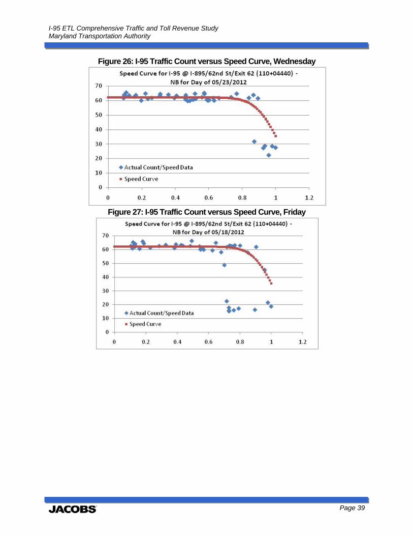
I-95 ETL Comprehensive Traffic and Toll Revenue Study Maryland Transportation Authority
Page 39
Figure 26: I-95 Traffic Count versus Speed Curve, Wednesday
Figure 27: I-95 Traffic Count versus Speed Curve, Friday
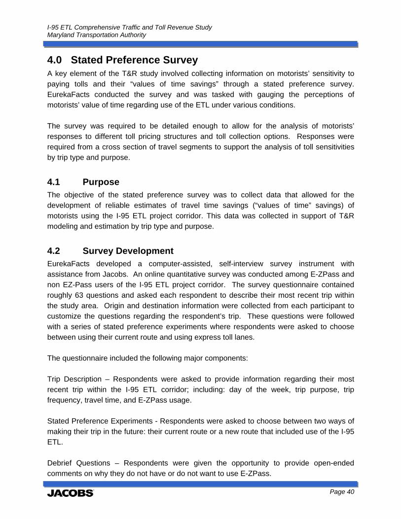
I-95 ETL Comprehensive Traffic and Toll Revenue Study Maryland Transportation Authority
Page 40
4.0 Stated Preference Survey A key element of the T&R study involved collecting information on motorists’ sensitivity to paying tolls and their “values of time savings” through a stated preference survey. EurekaFacts conducted the survey and was tasked with gauging the perceptions of motorists’ value of time regarding use of the ETL under various conditions. The survey was required to be detailed enough to allow for the analysis of motorists’ responses to different toll pricing structures and toll collection options. Responses were required from a cross section of travel segments to support the analysis of toll sensitivities by trip type and purpose.
4.1 Purpose The objective of the stated preference survey was to collect data that allowed for the development of reliable estimates of travel time savings (“values of time” savings) of motorists using the I-95 ETL project corridor. This data was collected in support of T&R modeling and estimation by trip type and purpose.
4.2 Survey Development EurekaFacts developed a computer-assisted, self-interview survey instrument with assistance from Jacobs. An online quantitative survey was conducted among E-ZPass and non EZ-Pass users of the I-95 ETL project corridor. The survey questionnaire contained roughly 63 questions and asked each respondent to describe their most recent trip within the study area. Origin and destination information were collected from each participant to customize the questions regarding the respondent’s trip. These questions were followed with a series of stated preference experiments where respondents were asked to choose between using their current route and using express toll lanes. The questionnaire included the following major components: Trip Description – Respondents were asked to provide information regarding their most recent trip within the I-95 ETL corridor; including: day of the week, trip purpose, trip frequency, travel time, and E-ZPass usage. Stated Preference Experiments - Respondents were asked to choose between two ways of making their trip in the future: their current route or a new route that included use of the I-95 ETL. Debrief Questions – Respondents were given the opportunity to provide open-ended comments on why they do not have or do not want to use E-ZPass.
I-95 ETL Comprehensive Traffic and Toll Revenue Study Maryland Transportation Authority
Page 41
Demographics – The survey also contained a series of questions to collect demographic data such as gender, employment status and income that EurekaFacts used to determine different segments.
4.3 Survey Results A brief summary of survey results is presented here. More detailed information is provided in the full stated preference survey report in Appendix B. Data collection took place between November 1, 2012 and November 16, 2012 and EurekaFacts obtained responses from 3,390 respondents. The survey yielded an overall response rate of 19% which was within the expected target range. Responses by group were: 22% among commercial vehicles, 43% among E-ZPass users and 5% among non E-ZPass users. EurekaFacts conducted statistical analysis and multinomial logit model estimation to derive value of time results for E-ZPass and non EZ-Pass users by trip type and purpose. The following summarizes the key value of time findings:
Value of time for E-ZPass users during peak hours was estimated at $16.90; 37% of E-ZPass users stated a clear preference for the I-95 ETL. Value of time for E-ZPass users during off-peak hours was estimated at $10.46; 27% of E-ZPass users stated a clear preference for the I-95 ETL. Value of time for non E-ZPass was estimated at $7.79; 25% of non E-ZPass users stated a clear preference for the I-95 ETL. Value of time for E-ZPass users during peak hours for commuting to / from work or work-related travel was estimated at $17.51; 37% of E-ZPass users stated a clear preference for I-95 ETL. Value of time for E-ZPass users during off-peak hours for commuting to / from work or work-related travel as estimated at $11.57; 29% of E-ZPass users stated a clear preference for I-95 ETL. Value of time for E-ZPass users during peak hours for non-work-related travel was estimated at $10.93; 26% of E-ZPass users stated a clear preference for the I-95 ETL. Value of time for E-ZPass users during off-peak hours for non-work-related travel was estimated at $10.46; 27% of E-ZPass users stated a clear preference for the I-95 ETL.
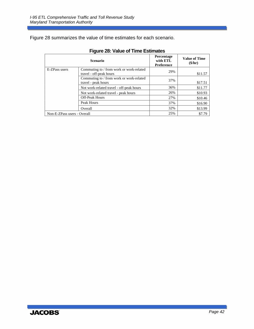
I-95 ETL Comprehensive Traffic and Toll Revenue Study Maryland Transportation Authority
Page 42
Figure 28 summarizes the value of time estimates for each scenario.
Figure 28: Value of Time Estimates
Scenario Percentage with ETL Preference
Value of Time ($/hr)
E-ZPass users Commuting to / from work or work-related travel - off-peak hours
29% $11.57
Commuting to / from work or work-related travel - peak hours
37% $17.51
Not work-related travel - off-peak hours 36% $11.77
Not work-related travel - peak hours 26% $10.93 Off-Peak Hours 27% $10.46 Peak Hours 37% $16.90
Overall 32% $13.99
Non-E-ZPass users - Overall 25% $7.79
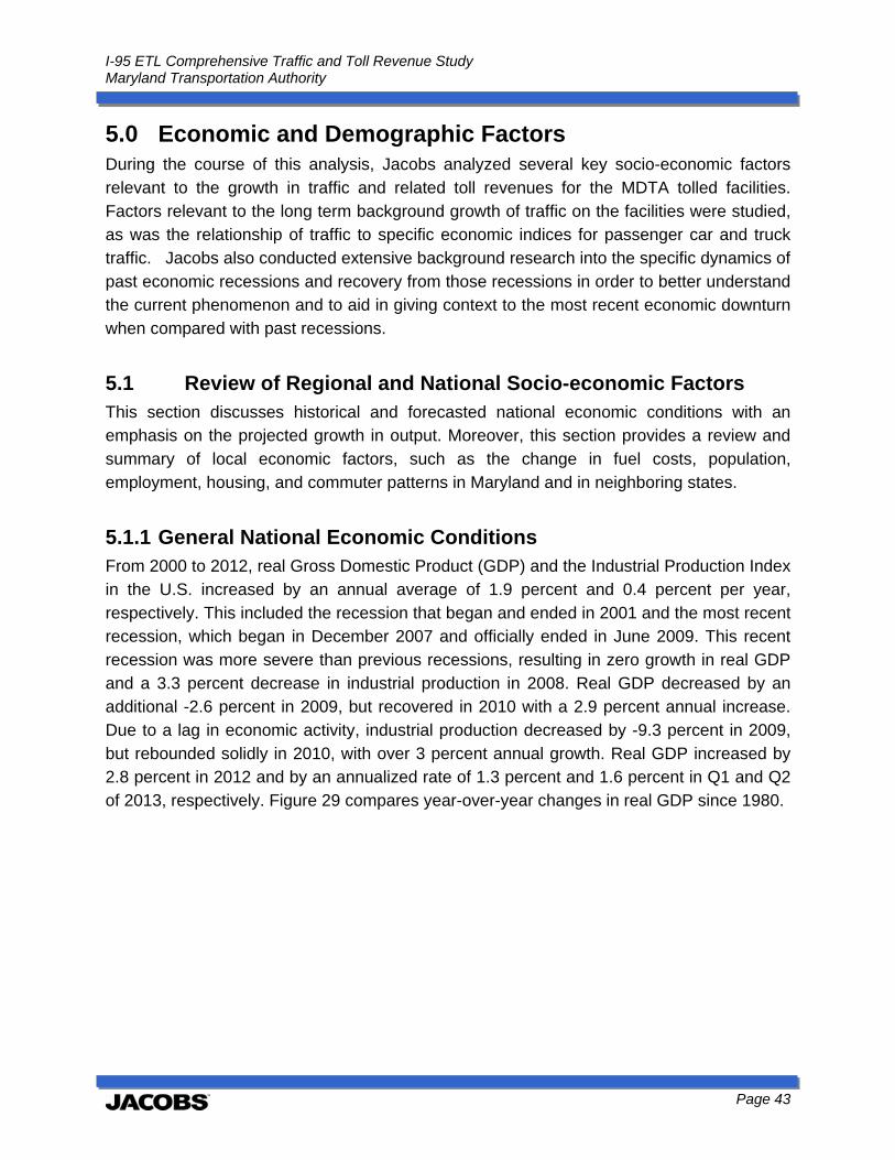
I-95 ETL Comprehensive Traffic and Toll Revenue Study Maryland Transportation Authority
Page 43
5.0 Economic and Demographic Factors During the course of this analysis, Jacobs analyzed several key socio-economic factors relevant to the growth in traffic and related toll revenues for the MDTA tolled facilities. Factors relevant to the long term background growth of traffic on the facilities were studied, as was the relationship of traffic to specific economic indices for passenger car and truck traffic. Jacobs also conducted extensive background research into the specific dynamics of past economic recessions and recovery from those recessions in order to better understand the current phenomenon and to aid in giving context to the most recent economic downturn when compared with past recessions.
5.1 Review of Regional and National Socio-economic Factors This section discusses historical and forecasted national economic conditions with an emphasis on the projected growth in output. Moreover, this section provides a review and summary of local economic factors, such as the change in fuel costs, population, employment, housing, and commuter patterns in Maryland and in neighboring states.
5.1.1 General National Economic Conditions From 2000 to 2012, real Gross Domestic Product (GDP) and the Industrial Production Index in the U.S. increased by an annual average of 1.9 percent and 0.4 percent per year, respectively. This included the recession that began and ended in 2001 and the most recent recession, which began in December 2007 and officially ended in June 2009. This recent recession was more severe than previous recessions, resulting in zero growth in real GDP and a 3.3 percent decrease in industrial production in 2008. Real GDP decreased by an additional -2.6 percent in 2009, but recovered in 2010 with a 2.9 percent annual increase. Due to a lag in economic activity, industrial production decreased by -9.3 percent in 2009, but rebounded solidly in 2010, with over 3 percent annual growth. Real GDP increased by 2.8 percent in 2012 and by an annualized rate of 1.3 percent and 1.6 percent in Q1 and Q2 of 2013, respectively. Figure 29 compares year-over-year changes in real GDP since 1980.
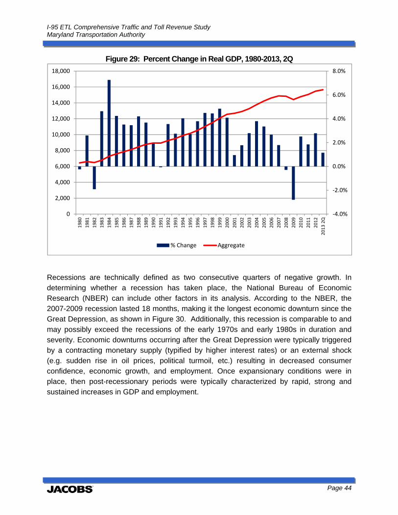
I-95 ETL Comprehensive Traffic and Toll Revenue Study Maryland Transportation Authority
Page 44
Figure 29: Percent Change in Real GDP, 1980-2013, 2Q
Recessions are technically defined as two consecutive quarters of negative growth. In determining whether a recession has taken place, the National Bureau of Economic Research (NBER) can include other factors in its analysis. According to the NBER, the 2007-2009 recession lasted 18 months, making it the longest economic downturn since the Great Depression, as shown in Figure 30. Additionally, this recession is comparable to and may possibly exceed the recessions of the early 1970s and early 1980s in duration and severity. Economic downturns occurring after the Great Depression were typically triggered by a contracting monetary supply (typified by higher interest rates) or an external shock (e.g. sudden rise in oil prices, political turmoil, etc.) resulting in decreased consumer confidence, economic growth, and employment. Once expansionary conditions were in place, then post-recessionary periods were typically characterized by rapid, strong and sustained increases in GDP and employment.
‐4.0%
‐2.0%
0.0%
2.0%
4.0%
6.0%
8.0%
0
2,000
4,000
6,000
8,000
10,000
12,000
14,000
16,000
18,000
1980
1981
1982
1983
1984
1985
1986
1987
1988
1989
1990
1991
1992
1993
1994
1995
1996
1997
1998
1999
2000
2001
2002
2003
2004
2005
2006
2007
2008
2009
2010
2011
2012
2013 2Q
% Change Aggregate
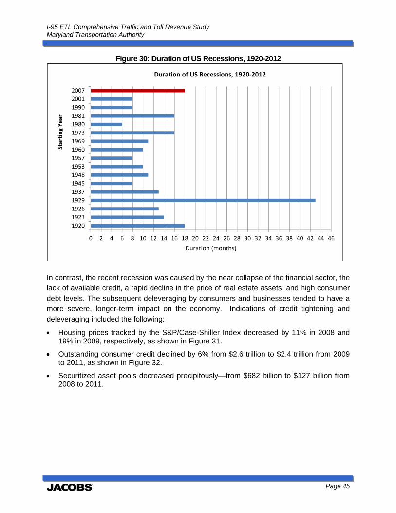
I-95 ETL Comprehensive Traffic and Toll Revenue Study Maryland Transportation Authority
Page 45
Figure 30: Duration of US Recessions, 1920-2012
In contrast, the recent recession was caused by the near collapse of the financial sector, the lack of available credit, a rapid decline in the price of real estate assets, and high consumer debt levels. The subsequent deleveraging by consumers and businesses tended to have a more severe, longer-term impact on the economy. Indications of credit tightening and deleveraging included the following:
Housing prices tracked by the S&P/Case-Shiller Index decreased by 11% in 2008 and 19% in 2009, respectively, as shown in Figure 31.
Outstanding consumer credit declined by 6% from $2.6 trillion to $2.4 trillion from 2009 to 2011, as shown in Figure 32.
Securitized asset pools decreased precipitously—from $682 billion to $127 billion from 2008 to 2011.
0 2 4 6 8 10 12 14 16 18 20 22 24 26 28 30 32 34 36 38 40 42 44 46
1920
1923
1926
1929
1937
1945
1948
1953
1957
1960
1969
1973
1980
1981
1990
2001
2007
Duration (months)
Starting Year
Duration of US Recessions, 1920‐2012
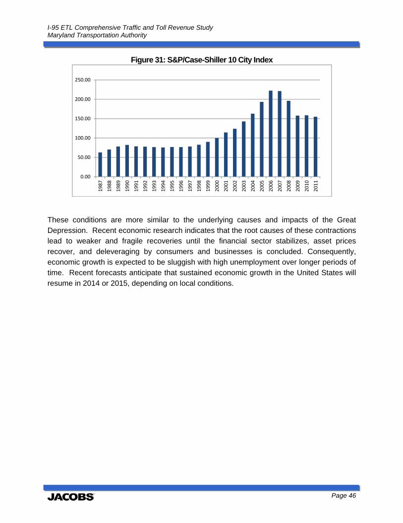
I-95 ETL Comprehensive Traffic and Toll Revenue Study Maryland Transportation Authority
Page 46
Figure 31: S&P/Case-Shiller 10 City Index
These conditions are more similar to the underlying causes and impacts of the Great Depression. Recent economic research indicates that the root causes of these contractions lead to weaker and fragile recoveries until the financial sector stabilizes, asset prices recover, and deleveraging by consumers and businesses is concluded. Consequently, economic growth is expected to be sluggish with high unemployment over longer periods of time. Recent forecasts anticipate that sustained economic growth in the United States will resume in 2014 or 2015, depending on local conditions.
0.00
50.00
100.00
150.00
200.00
250.00
1987
1988
1989
1990
1991
1992
1993
1994
1995
1996
1997
1998
1999
2000
2001
2002
2003
2004
2005
2006
2007
2008
2009
2010
2011
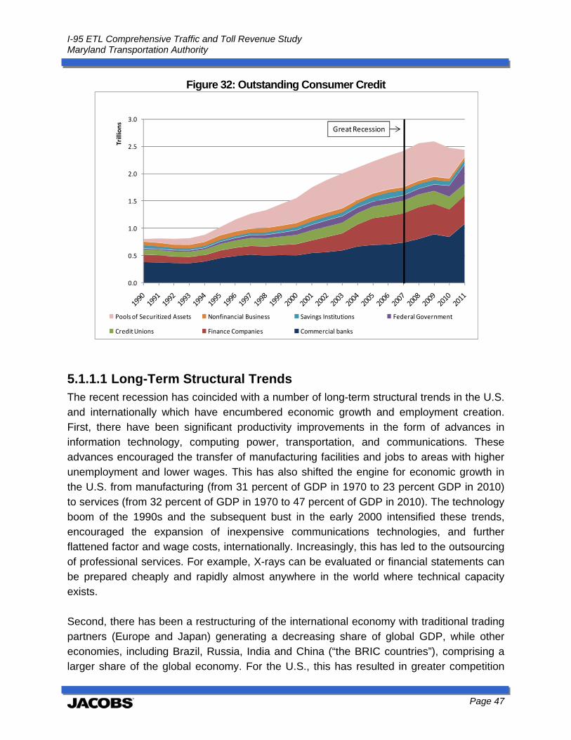
I-95 ETL Comprehensive Traffic and Toll Revenue Study Maryland Transportation Authority
Page 47
Figure 32: Outstanding Consumer Credit
5.1.1.1 Long-Term Structural Trends The recent recession has coincided with a number of long-term structural trends in the U.S. and internationally which have encumbered economic growth and employment creation. First, there have been significant productivity improvements in the form of advances in information technology, computing power, transportation, and communications. These advances encouraged the transfer of manufacturing facilities and jobs to areas with higher unemployment and lower wages. This has also shifted the engine for economic growth in the U.S. from manufacturing (from 31 percent of GDP in 1970 to 23 percent GDP in 2010) to services (from 32 percent of GDP in 1970 to 47 percent of GDP in 2010). The technology boom of the 1990s and the subsequent bust in the early 2000 intensified these trends, encouraged the expansion of inexpensive communications technologies, and further flattened factor and wage costs, internationally. Increasingly, this has led to the outsourcing of professional services. For example, X-rays can be evaluated or financial statements can be prepared cheaply and rapidly almost anywhere in the world where technical capacity exists. Second, there has been a restructuring of the international economy with traditional trading partners (Europe and Japan) generating a decreasing share of global GDP, while other economies, including Brazil, Russia, India and China (“the BRIC countries”), comprising a larger share of the global economy. For the U.S., this has resulted in greater competition
0.0
0.5
1.0
1.5
2.0
2.5
3.0Trillions
Pools of Securitized Assets Nonfinancial Business Savings Institutions Federal Government
Credit Unions Finance Companies Commercial banks
Great Recession
I-95 ETL Comprehensive Traffic and Toll Revenue Study Maryland Transportation Authority
Page 48
not just in manufacturing, but also in professional services, reducing direct and indirect employment. A third trend has been the aging of the U.S population. The median age has increased from 27.9 in 1970 to 37.2 in 2010. This trend has also taken hold in Europe and Japan and is expected to eventually impact China due to its one-child policy. Finally, there has been a rapid and significant expansion in consumer credit, which has reached unsustainable levels. As a result, consumers have reduced or deferred large discretionary purchases, such as vehicles and appliances, until debt levels have decreased to more manageable levels. These factors tend to further dampen economic growth and employment over the short-term.
5.1.1.2 Short-Term Economic Forecast In early 2012, there was modest enthusiasm with respect to economic growth and employment, which has decreased slightly as the year has progressed. Forecasts prepared in August 2012 have reduced the forecasted growth in real GDP. The median of selected economic forecasts developed by financial institutions and industry analysts for real GDP in August 2012 (see Figure 12) was 1.7 percent, down from 2.2 percent at the start of the year. The spread among forecasts (50+ observations) is relatively small, ranging from 1.9 percent to 2.5 percent. For 2013, the consensus forecast was that real GDP would increase by 2.1 percent, albeit with a wider range—0.9 percent to 3.7 percent. Factors that may negatively impact real GDP in the short-term include the following:
Recessionary conditions in Europe due to the weak fiscal position of Greece, Portugal, Spain, and Italy and concerns about the stability of the Euro;
Signs of decreased economic growth in Brazil and China;
The currently scheduled $500 billion budget cuts and/or tax increases at the end of 2012. The U.S. Congressional Budget Office (CBO) warned that the upcoming “fiscal cliff” could result in a return to recessionary conditions; and
Increased tensions in the Middle East. The previous and revised forecast of Real GDP for 2012 and 2013 are presented in Figure 33 and Figure 34, respectively. (As of this writing, the U.S. Federal Reserve Bank (FRB) and the International Monetary Fund (IMF) have not yet revised their forecasts.) Factors cited in these revised forecasts include slower than expected economic growth, higher than expected unemployment, flattened consumer spending, weakness in the housing market and new construction, stock market volatility, and the recent downgrade in the U.S. credit
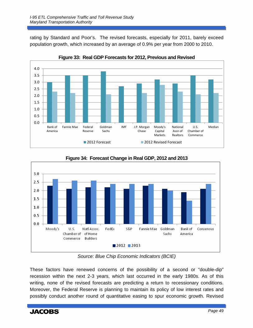
I-95 ETL Comprehensive Traffic and Toll Revenue Study Maryland Transportation Authority
Page 49
rating by Standard and Poor’s. The revised forecasts, especially for 2011, barely exceed population growth, which increased by an average of 0.9% per year from 2000 to 2010.
Figure 33: Real GDP Forecasts for 2012, Previous and Revised
Figure 34: Forecast Change in Real GDP, 2012 and 2013
Source: Blue Chip Economic Indicators (BCIE)
These factors have renewed concerns of the possibility of a second or “double-dip” recession within the next 2-3 years, which last occurred in the early 1980s. As of this writing, none of the revised forecasts are predicting a return to recessionary conditions. Moreover, the Federal Reserve is planning to maintain its policy of low interest rates and possibly conduct another round of quantitative easing to spur economic growth. Revised
0.0
0.5
1.0
1.5
2.0
2.5
3.0
3.5
4.0
Bank ofAmerica
Fannie Mae FederalReserve
GoldmanSachs
IMF J.P. MorganChase
Moody'sCapitalMarkets
NationalAssn ofRealtors
U.S.Chamber ofCommerce
Median
2012 Forecast 2012 Revised Forecast
I-95 ETL Comprehensive Traffic and Toll Revenue Study Maryland Transportation Authority
Page 50
forecasts are generally calling for sluggish economic growth and weak labor market conditions in 2011 with a slight improvement in 2012. Possible signs of a second recession have also not yet materialized. For example, the yield curve remains positive with short term interest rates (0-12 months) on U.S. Treasuries trading at or near zero and the interest rates on 30-year U.S. Treasuries trading at 3.75%, as of August 23, 2011. Additionally, the market for crude oil remains strong with the price expected to be close to $100/barrel for this year and next. In comparison, the price during 2009, which corresponded to the steepest part of the recession, averaged approximately $62/barrel. If the forecasts calling for continued slow growth materialize, then the economy will remain vulnerable to exogenous risks, which could potentially drive the U.S. economy back into recession. External events that could bring on a second recession include the ongoing European debt crises, continued volatility in the stock market which reduces investor and consumer confidence, continued instability in the Middle East, or a natural disaster (e.g. the 2011 earthquake in Japan). In particular, the European debt situation represents a key external risk that could affect economic recovery in the U.S. At the present time, there are concerns that Ireland, Portugal or Spain may join Greece in requiring assistance from the European Union or the IMF in order to avoid default. French banks are particularly exposed, which could result in a second round of financial contagion, further retrenchment in the financial sector, and another recession. The consensus outlook of macroeconomic analysts at financial institutions and business associations is that real U.S. GDP is expected to increase on an annualized basis by 1.5 percent and 2.6 percent during 2013 and 2014, respectively. The consensus forecast for the industrial production index is a 2.5 percent increase in 2013 and 3.2 percent increase in 2014. It is anticipated that a slow recovery will emerge in the medium term in contrast to robust recoveries of previous recessions. This fits with the current base case forecast provided by Jacobs for the MDTA facilities.
5.1.1.3 Industrial Production Changes in U.S. industrial production have historically moved in tandem with GDP, albeit with steeper decreases during recessions and larger increases during recovery periods. During the lowest point of the 2001 recession, the Industrial Production Index (IPI) decreased by 4.0 percent as shown in Figure 35. Due to the severity of the 2007-2009 recession, IPI declined -13.5 percent in 2009. Since then, IPI has recovered increasing by 5.4 percent and 3.4 percent during 2010 and 2011, respectively. Despite this recovery, the gross value of the IPI for “Final Products and Non-Industrial Supplies” is at 97 percent of its 2007 peak.
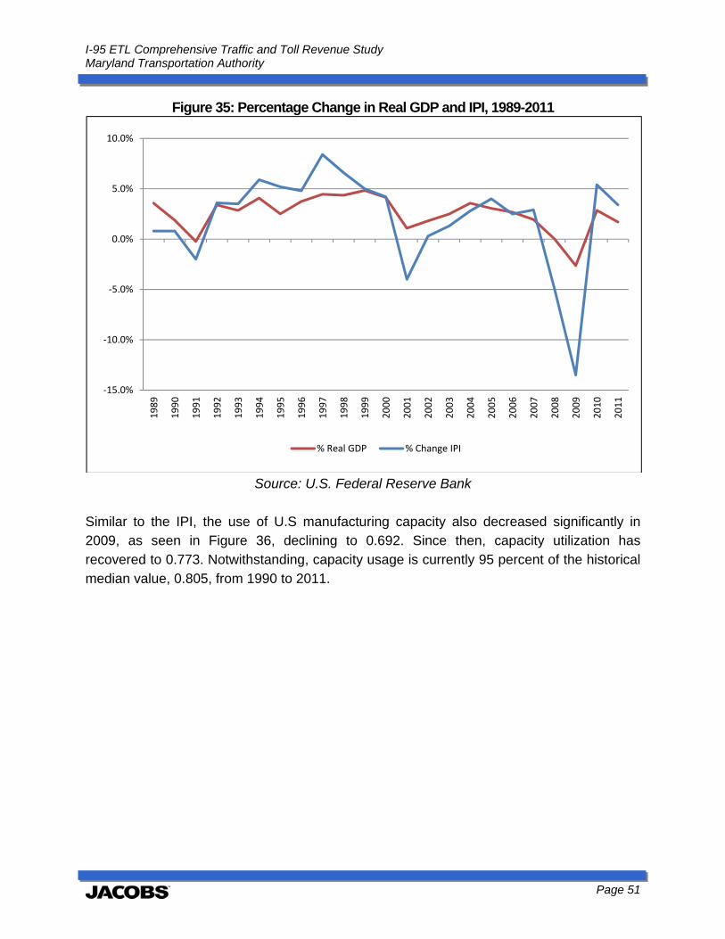
I-95 ETL Comprehensive Traffic and Toll Revenue Study Maryland Transportation Authority
Page 51
Figure 35: Percentage Change in Real GDP and IPI, 1989-2011
Source: U.S. Federal Reserve Bank
Similar to the IPI, the use of U.S manufacturing capacity also decreased significantly in 2009, as seen in Figure 36, declining to 0.692. Since then, capacity utilization has recovered to 0.773. Notwithstanding, capacity usage is currently 95 percent of the historical median value, 0.805, from 1990 to 2011.
‐15.0%
‐10.0%
‐5.0%
0.0%
5.0%
10.0%
1989
1990
1991
1992
1993
1994
1995
1996
1997
1998
1999
2000
2001
2002
2003
2004
2005
2006
2007
2008
2009
2010
2011
% Real GDP % Change IPI

I-95 ETL Comprehensive Traffic and Toll Revenue Study Maryland Transportation Authority
Page 52
Figure 36: Capacity Utilization, 1990-2011
Source: U.S. Federal Reserve Bank
5.1.1.4 Industrial Production Forecasts Based on forecasts developed by financial institutions and industry analysts, the Industrial Production Index (IPI) is forecasted to increase by 4.1 percent in 2012 and 2.8 percent in 2013. This slower forecast likely captures the decrease in exports due to the recessionary conditions in Europe and slower growth in emerging markets, including Brazil and China. Selected forecasts are shown in Figure 37.
0.000
0.100
0.200
0.300
0.400
0.500
0.600
0.700
0.800
0.900
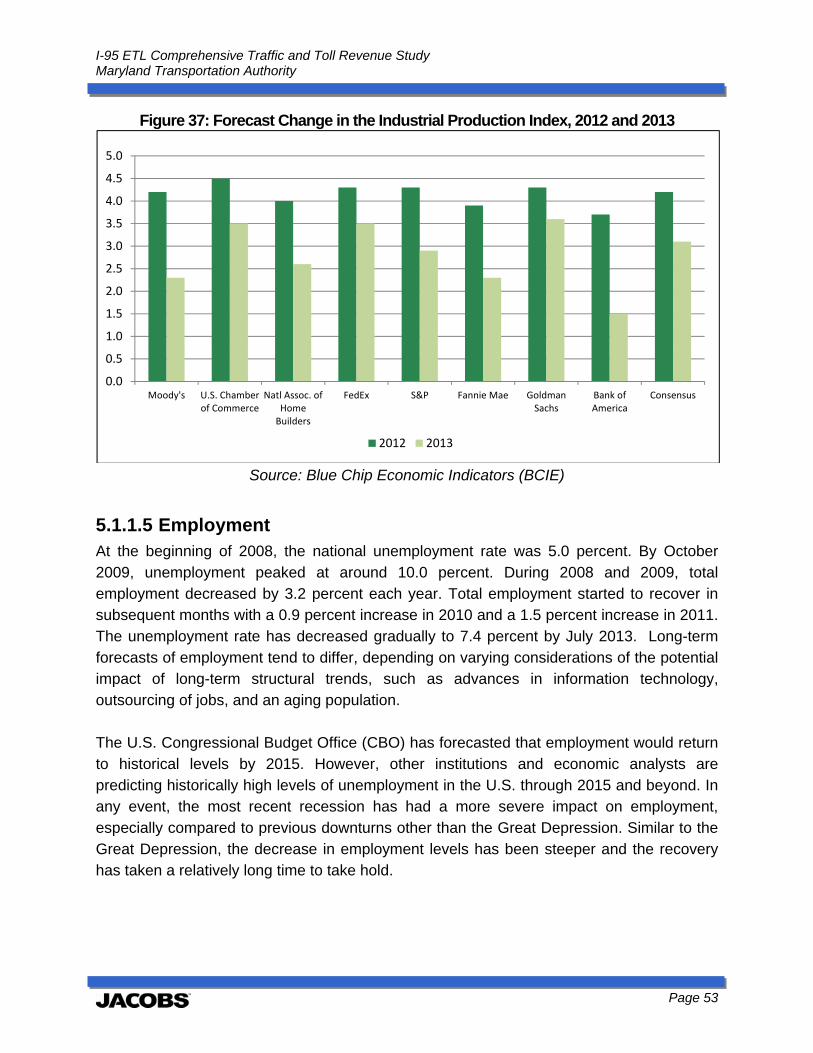
I-95 ETL Comprehensive Traffic and Toll Revenue Study Maryland Transportation Authority
Page 53
Figure 37: Forecast Change in the Industrial Production Index, 2012 and 2013
Source: Blue Chip Economic Indicators (BCIE)
5.1.1.5 Employment At the beginning of 2008, the national unemployment rate was 5.0 percent. By October 2009, unemployment peaked at around 10.0 percent. During 2008 and 2009, total employment decreased by 3.2 percent each year. Total employment started to recover in subsequent months with a 0.9 percent increase in 2010 and a 1.5 percent increase in 2011. The unemployment rate has decreased gradually to 7.4 percent by July 2013. Long-term forecasts of employment tend to differ, depending on varying considerations of the potential impact of long-term structural trends, such as advances in information technology, outsourcing of jobs, and an aging population. The U.S. Congressional Budget Office (CBO) has forecasted that employment would return to historical levels by 2015. However, other institutions and economic analysts are predicting historically high levels of unemployment in the U.S. through 2015 and beyond. In any event, the most recent recession has had a more severe impact on employment, especially compared to previous downturns other than the Great Depression. Similar to the Great Depression, the decrease in employment levels has been steeper and the recovery has taken a relatively long time to take hold.
0.0
0.5
1.0
1.5
2.0
2.5
3.0
3.5
4.0
4.5
5.0
Moody's U.S. Chamberof Commerce
Natl Assoc. ofHomeBuilders
FedEx S&P Fannie Mae GoldmanSachs
Bank ofAmerica
Consensus
2012 2013
I-95 ETL Comprehensive Traffic and Toll Revenue Study Maryland Transportation Authority
Page 54
5.1.2 National Trends in Vehicle Miles Traveled (VMT) The United States has experienced a never-before-seen flattening, then drop, in vehicle-miles traveled (VMT) on its highways over the past several years. A reduction in VMT means less revenue – in the form of gas tax or tolls - for funding transportation projects. Jacobs reviewed and compiled available reports and data to investigate the possible factors contributing to this phenomenon. Figure 38 depicts the 12-month moving total of national travel mileage from 1940 through July 2012 on all U.S. highways. As seen in this figure, there were temporary reductions in VMT during World War II, oil crises and economic recessions. Despite these temporary “dips”, the VMT continued to grow rapidly over the years. It shows that, in recent years, with the exception of short, flat periods during the 1991 and 2001 recessions (each less than one year), VMT grew at a steady pace through about 2005. VMT then grew at a much slower pace through 2008. The increase in gas prices and the downturn in economic activity that took hold in late 2008 resulted in a significant reduction in total national travel mileage after December 2007 peak. While VMT declined throughout 2008, it has remained flat in 2009 until the summer months, when there was a slight increase of 0.9 percent over the previous year. This perceived growth was due in part to the large reduction in summer gas prices from 2008 to 2009. Since the recession ended, there have been slight increases and decreases in VMT from month to month with an average annual increase of about 0.9 percent between 2010 and 2012. For the first two quarters of 2013, VMT remained unchanged during Q1 and decreased slightly by 0.2 percent in Q2 over the previous year.
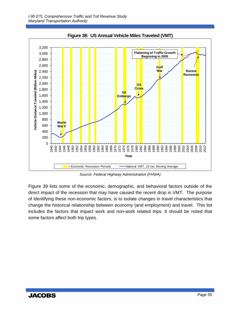
I-95 ETL Comprehensive Traffic and Toll Revenue Study Maryland Transportation Authority
Page 55
Figure 38: US Annual Vehicle Miles Traveled (VMT)
Source: Federal Highway Administration (FHWA)
Figure 39 lists some of the economic, demographic, and behavioral factors outside of the direct impact of the recession that may have caused the recent drop in VMT. The purpose of identifying these non-economic factors, is to isolate changes in travel characteristics that change the historical relationship between economy (and employment) and travel. This list includes the factors that impact work and non-work related trips. It should be noted that some factors affect both trip types.
0
200
400
600
800
1,000
1,200
1,400
1,600
1,800
2,000
2,200
2,400
2,600
2,800
3,000
3,20019
4019
4219
4419
4619
4819
5019
5219
5419
5619
5819
6019
6219
6419
6619
6819
7019
7219
7419
7619
7819
8019
8219
8419
8619
8819
9019
9219
9419
9619
9820
0020
0220
0420
0620
0820
1020
12
Veh
icle
-Dis
tan
ce T
rave
led
(B
illio
n M
iles)
Year
= Economic Recession Periods National VMT, 12-mo. Moving Average
Oil Embargo
Gulf War
Oil Crisis
World War II
Recent Recession
Flattening of Traffic Growth Beginning in 2005
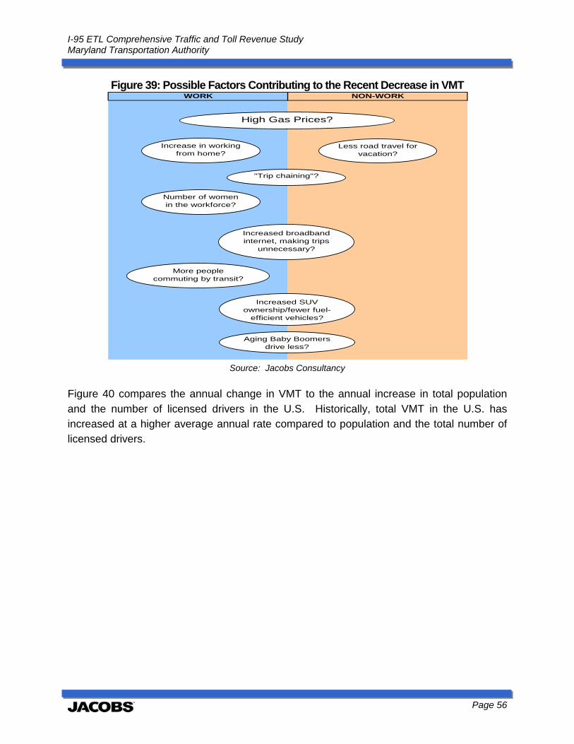
I-95 ETL Comprehensive Traffic and Toll Revenue Study Maryland Transportation Authority
Page 56
Figure 39: Possible Factors Contributing to the Recent Decrease in VMT
Source: Jacobs Consultancy
Figure 40 compares the annual change in VMT to the annual increase in total population and the number of licensed drivers in the U.S. Historically, total VMT in the U.S. has increased at a higher average annual rate compared to population and the total number of licensed drivers.
WORK NON-WORK
High Gas Prices?
Number of women in the workforce?
Less road travel for vacation?
"Trip chaining"?
Increase in working from home?
Increased broadband internet, making trips
unnecessary?
More people commuting by transit?
Increased SUV ownership/fewer fuel-
efficient vehicles?
Aging Baby Boomers drive less?
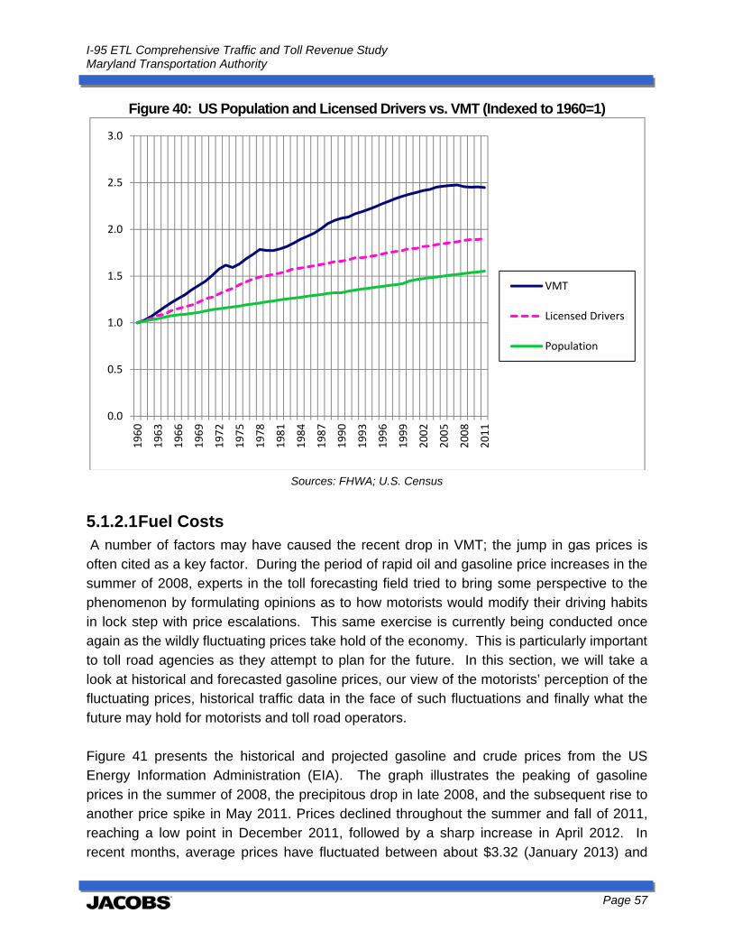
I-95 ETL Comprehensive Traffic and Toll Revenue Study Maryland Transportation Authority
Page 57
Figure 40: US Population and Licensed Drivers vs. VMT (Indexed to 1960=1)
Sources: FHWA; U.S. Census
5.1.2.1 Fuel Costs A number of factors may have caused the recent drop in VMT; the jump in gas prices is often cited as a key factor. During the period of rapid oil and gasoline price increases in the summer of 2008, experts in the toll forecasting field tried to bring some perspective to the phenomenon by formulating opinions as to how motorists would modify their driving habits in lock step with price escalations. This same exercise is currently being conducted once again as the wildly fluctuating prices take hold of the economy. This is particularly important to toll road agencies as they attempt to plan for the future. In this section, we will take a look at historical and forecasted gasoline prices, our view of the motorists’ perception of the fluctuating prices, historical traffic data in the face of such fluctuations and finally what the future may hold for motorists and toll road operators. Figure 41 presents the historical and projected gasoline and crude prices from the US Energy Information Administration (EIA). The graph illustrates the peaking of gasoline prices in the summer of 2008, the precipitous drop in late 2008, and the subsequent rise to another price spike in May 2011. Prices declined throughout the summer and fall of 2011, reaching a low point in December 2011, followed by a sharp increase in April 2012. In recent months, average prices have fluctuated between about $3.32 (January 2013) and
0.0
0.5
1.0
1.5
2.0
2.5
3.01960
1963
1966
1969
1972
1975
1978
1981
1984
1987
1990
1993
1996
1999
2002
2005
2008
2011
VMT
Licensed Drivers
Population
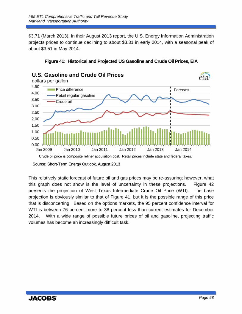
I-95 ETL Comprehensive Traffic and Toll Revenue Study Maryland Transportation Authority
Page 58
$3.71 (March 2013). In their August 2013 report, the U.S. Energy Information Administration projects prices to continue declining to about $3.31 in early 2014, with a seasonal peak of about $3.51 in May 2014.
Figure 41: Historical and Projected US Gasoline and Crude Oil Prices, EIA
This relatively static forecast of future oil and gas prices may be re-assuring; however, what this graph does not show is the level of uncertainty in these projections. Figure 42 presents the projection of West Texas Intermediate Crude Oil Price (WTI). The base projection is obviously similar to that of Figure 41, but it is the possible range of this price that is disconcerting. Based on the options markets, the 95 percent confidence interval for WTI is between 76 percent more to 38 percent less than current estimates for December 2014. With a wide range of possible future prices of oil and gasoline, projecting traffic volumes has become an increasingly difficult task.
Forecast
0.00
0.50
1.00
1.50
2.00
2.50
3.00
3.50
4.00
4.50
Jan 2009 Jan 2010 Jan 2011 Jan 2012 Jan 2013 Jan 2014
U.S. Gasoline and Crude Oil Pricesdollars per gallon
Price difference
Retail regular gasoline
Crude oil
Source: Short-Term Energy Outlook, August 2013
Crude oil price is composite refiner acquisition cost. Retail prices include state and federal taxes.
Source: Short-Term Energy Outlook, August 2013
Crude oil price is composite refiner acquisition cost. Retail prices include state and federal taxes.

I-95 ETL Comprehensive Traffic and Toll Revenue Study Maryland Transportation Authority
Page 59
Figure 42: Historical and Projected Crude Oil Prices with Confidence Range, EIA
Another consideration is the decreasing reliance on oil and gasoline as the fuel for our vehicles with the increasing fuel efficiency of vehicles, as shown in Figure 43. The sharp increase in fuel efficiency in the late 1970s was caused by the oil crisis and the trend toward buying smaller, more fuel-efficient vehicles. A gradual decline in average MPG from 1987 through 2004 occurred as larger vehicles and SUVs became more popular. From 2005 through today, that trend was again turned around, and today vehicles are more fuel-efficient than ever. This means that, generally speaking, gas prices today do not have as large an effect on drivers as it did ten years ago. Also to consider in this discussion is the emergence and growth of hybrid and electric vehicles in the marketplace. These alternate fuel vehicles, while they of course rely on some sort of fuel source, may not be so dependent on oil in the future and a wider range of energy options from natural gas, coal, nuclear and possibly renewable sources such as solar and wind. It has been estimated that electric vehicles could constitute up to 35 percent of the market by 2025. Though these predictions vary widely by source, what is important to understand is the potential for mitigation of rising oil prices by motorists. Also important to note is that the U.S. crude oil production has increased since 2008, reversing a decline that began in 1986. From 5 million barrels per day in 2008, U.S. crude oil production increased by 30 percent to 6.5 million barrels per day in 2012. Improvements in advanced crude oil production technologies continue to lift domestic supply, with the U.S. Energy Information Administration projecting production to increase at an annual rate of 1.9% to 7.5 million barrels per day by 2020. The net import share of U.S. petroleum grew
020406080
100120140160180200220
Jan 2012 Jul 2012 Jan 2013 Jul 2013 Jan 2014 Jul 2014
West Texas Intermediate (WTI) Crude Oil Pricedollars per barrel
Historical spot priceSTEO price forecastNYMEX futures price95% NYMEX futures upper confidence interval95% NYMEX futures lower confidence interval
Source: Short-Term Energy Outlook, August 2013
Note: Confidence interval derived from options market information for the 5 trading days ending August 1, 2013. Intervals not calculated for months with sparse trading in near-the-money options contracts.
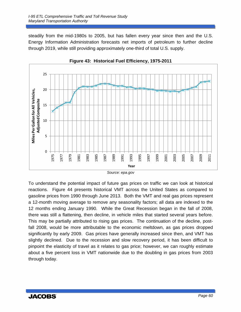
I-95 ETL Comprehensive Traffic and Toll Revenue Study Maryland Transportation Authority
Page 60
steadily from the mid-1980s to 2005, but has fallen every year since then and the U.S. Energy Information Administration forecasts net imports of petroleum to further decline through 2019, while still providing approximately one-third of total U.S. supply.
Figure 43: Historical Fuel Efficiency, 1975-2011
Source: epa.gov
To understand the potential impact of future gas prices on traffic we can look at historical reactions. Figure 44 presents historical VMT across the United States as compared to gasoline prices from 1990 through June 2013. Both the VMT and real gas prices represent a 12-month moving average to remove any seasonality factors; all data are indexed to the 12 months ending January 1990. While the Great Recession began in the fall of 2008, there was still a flattening, then decline, in vehicle miles that started several years before. This may be partially attributed to rising gas prices. The continuation of the decline, post-fall 2008, would be more attributable to the economic meltdown, as gas prices dropped significantly by early 2009. Gas prices have generally increased since then, and VMT has slightly declined. Due to the recession and slow recovery period, it has been difficult to pinpoint the elasticity of travel as it relates to gas price; however, we can roughly estimate about a five percent loss in VMT nationwide due to the doubling in gas prices from 2003 through today.
0
5
10
15
20
25
1975
1977
1979
1981
1983
1985
1987
1989
1991
1993
1995
1997
1999
2001
2003
2005
2007
2009
2011
Miles Per G
allon for A
ll Vehicles,
Adjusted Composite
Year
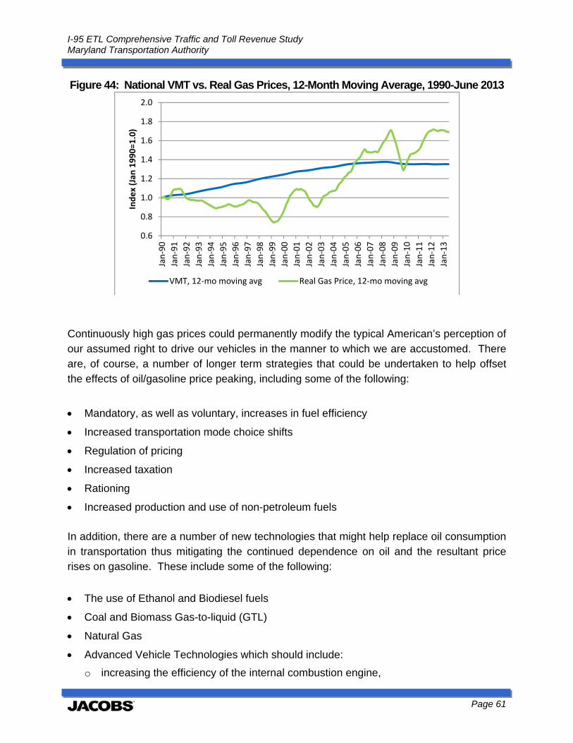
I-95 ETL Comprehensive Traffic and Toll Revenue Study Maryland Transportation Authority
Page 61
Figure 44: National VMT vs. Real Gas Prices, 12-Month Moving Average, 1990-June 2013
Continuously high gas prices could permanently modify the typical American’s perception of our assumed right to drive our vehicles in the manner to which we are accustomed. There are, of course, a number of longer term strategies that could be undertaken to help offset the effects of oil/gasoline price peaking, including some of the following:
Mandatory, as well as voluntary, increases in fuel efficiency
Increased transportation mode choice shifts
Regulation of pricing
Increased taxation
Rationing
Increased production and use of non-petroleum fuels In addition, there are a number of new technologies that might help replace oil consumption in transportation thus mitigating the continued dependence on oil and the resultant price rises on gasoline. These include some of the following:
The use of Ethanol and Biodiesel fuels
Coal and Biomass Gas-to-liquid (GTL)
Natural Gas
Advanced Vehicle Technologies which should include:
o increasing the efficiency of the internal combustion engine,
0.6
0.8
1.0
1.2
1.4
1.6
1.8
2.0
Jan‐90
Jan‐91
Jan‐92
Jan‐93
Jan‐94
Jan‐95
Jan‐96
Jan‐97
Jan‐98
Jan‐99
Jan‐00
Jan‐01
Jan‐02
Jan‐03
Jan‐04
Jan‐05
Jan‐06
Jan‐07
Jan‐08
Jan‐09
Jan‐10
Jan‐11
Jan‐12
Jan‐13
Index (Jan
1990=1.0)
VMT, 12‐mo moving avg Real Gas Price, 12‐mo moving avg
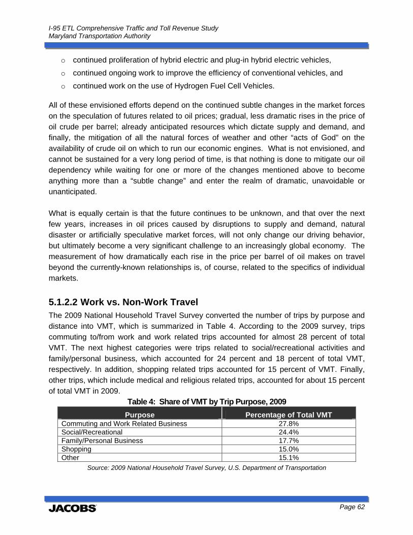
I-95 ETL Comprehensive Traffic and Toll Revenue Study Maryland Transportation Authority
Page 62
o continued proliferation of hybrid electric and plug-in hybrid electric vehicles,
o continued ongoing work to improve the efficiency of conventional vehicles, and
o continued work on the use of Hydrogen Fuel Cell Vehicles. All of these envisioned efforts depend on the continued subtle changes in the market forces on the speculation of futures related to oil prices; gradual, less dramatic rises in the price of oil crude per barrel; already anticipated resources which dictate supply and demand, and finally, the mitigation of all the natural forces of weather and other “acts of God” on the availability of crude oil on which to run our economic engines. What is not envisioned, and cannot be sustained for a very long period of time, is that nothing is done to mitigate our oil dependency while waiting for one or more of the changes mentioned above to become anything more than a “subtle change” and enter the realm of dramatic, unavoidable or unanticipated. What is equally certain is that the future continues to be unknown, and that over the next few years, increases in oil prices caused by disruptions to supply and demand, natural disaster or artificially speculative market forces, will not only change our driving behavior, but ultimately become a very significant challenge to an increasingly global economy. The measurement of how dramatically each rise in the price per barrel of oil makes on travel beyond the currently-known relationships is, of course, related to the specifics of individual markets.
5.1.2.2 Work vs. Non-Work Travel The 2009 National Household Travel Survey converted the number of trips by purpose and distance into VMT, which is summarized in Table 4. According to the 2009 survey, trips commuting to/from work and work related trips accounted for almost 28 percent of total VMT. The next highest categories were trips related to social/recreational activities and family/personal business, which accounted for 24 percent and 18 percent of total VMT, respectively. In addition, shopping related trips accounted for 15 percent of VMT. Finally, other trips, which include medical and religious related trips, accounted for about 15 percent of total VMT in 2009.
Table 4: Share of VMT by Trip Purpose, 2009
Purpose Percentage of Total VMT Commuting and Work Related Business 27.8% Social/Recreational 24.4% Family/Personal Business 17.7% Shopping 15.0% Other 15.1%
Source: 2009 National Household Travel Survey, U.S. Department of Transportation
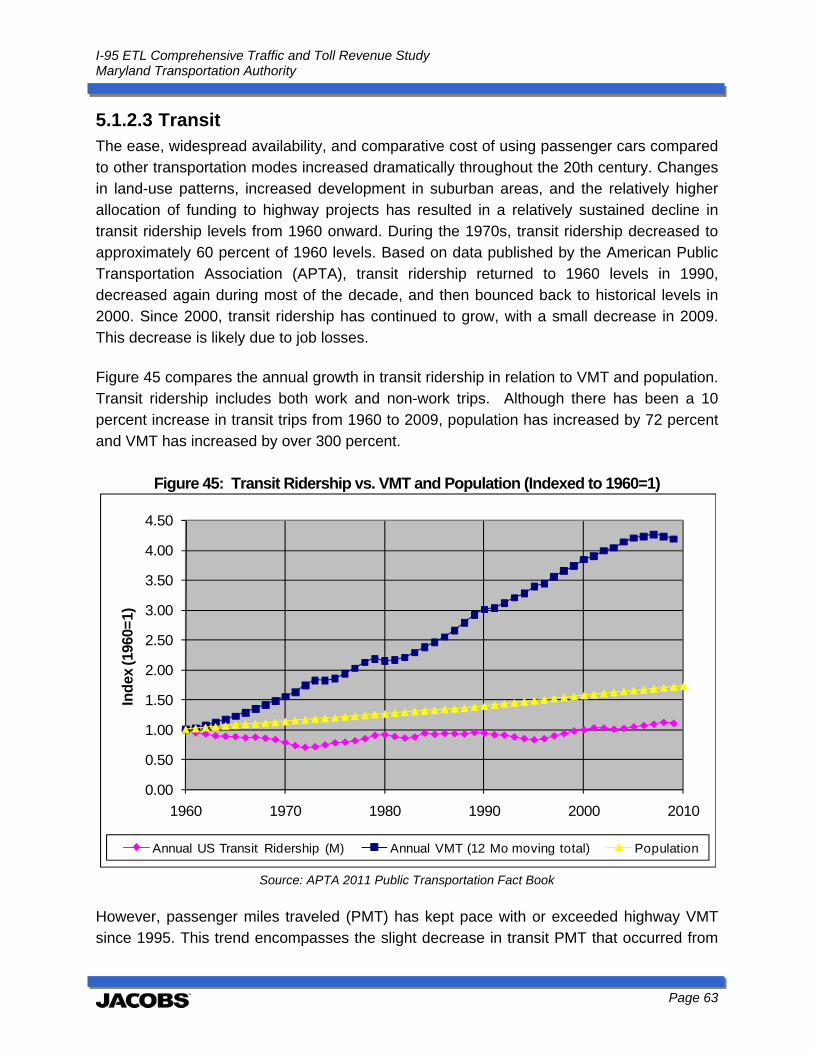
I-95 ETL Comprehensive Traffic and Toll Revenue Study Maryland Transportation Authority
Page 63
5.1.2.3 Transit The ease, widespread availability, and comparative cost of using passenger cars compared to other transportation modes increased dramatically throughout the 20th century. Changes in land-use patterns, increased development in suburban areas, and the relatively higher allocation of funding to highway projects has resulted in a relatively sustained decline in transit ridership levels from 1960 onward. During the 1970s, transit ridership decreased to approximately 60 percent of 1960 levels. Based on data published by the American Public Transportation Association (APTA), transit ridership returned to 1960 levels in 1990, decreased again during most of the decade, and then bounced back to historical levels in 2000. Since 2000, transit ridership has continued to grow, with a small decrease in 2009. This decrease is likely due to job losses. Figure 45 compares the annual growth in transit ridership in relation to VMT and population. Transit ridership includes both work and non-work trips. Although there has been a 10 percent increase in transit trips from 1960 to 2009, population has increased by 72 percent and VMT has increased by over 300 percent.
Figure 45: Transit Ridership vs. VMT and Population (Indexed to 1960=1)
Source: APTA 2011 Public Transportation Fact Book
However, passenger miles traveled (PMT) has kept pace with or exceeded highway VMT since 1995. This trend encompasses the slight decrease in transit PMT that occurred from
0.00
0.50
1.00
1.50
2.00
2.50
3.00
3.50
4.00
4.50
1960 1970 1980 1990 2000 2010
Ind
ex (1
960=
1)
Annual US Transit Ridership (M) Annual VMT (12 Mo moving total) Population
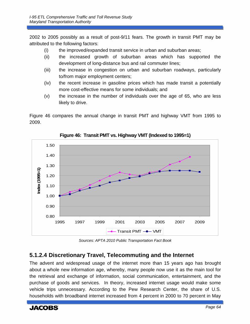
I-95 ETL Comprehensive Traffic and Toll Revenue Study Maryland Transportation Authority
Page 64
2002 to 2005 possibly as a result of post-9/11 fears. The growth in transit PMT may be attributed to the following factors:
(i) the improved/expanded transit service in urban and suburban areas; (ii) the increased growth of suburban areas which has supported the
development of long-distance bus and rail commuter lines; (iii) the increase in congestion on urban and suburban roadways, particularly
to/from major employment centers; (iv) the recent increase in gasoline prices which has made transit a potentially
more cost-effective means for some individuals; and (v) the increase in the number of individuals over the age of 65, who are less
likely to drive. Figure 46 compares the annual change in transit PMT and highway VMT from 1995 to 2009.
Figure 46: Transit PMT vs. Highway VMT (Indexed to 1995=1)
Sources: APTA 2010 Public Transportation Fact Book
5.1.2.4 Discretionary Travel, Telecommuting and the Internet The advent and widespread usage of the internet more than 15 years ago has brought about a whole new information age, whereby, many people now use it as the main tool for the retrieval and exchange of information, social communication, entertainment, and the purchase of goods and services. In theory, increased internet usage would make some vehicle trips unnecessary. According to the Pew Research Center, the share of U.S. households with broadband internet increased from 4 percent in 2000 to 70 percent in May
0.80
0.90
1.00
1.10
1.20
1.30
1.40
1.50
1995 1997 1999 2001 2003 2005 2007 2009
Index
(19
95=1)
Transit PMT VMT

I-95 ETL Comprehensive Traffic and Toll Revenue Study Maryland Transportation Authority
Page 65
2013. According to Nielsen Online, Americans currently spend an average of nearly 60 hours per month on the internet or about two hours per day. A 2000 study by the Stanford Institute for the Quantitative Study of Society (SIQSS) included a survey of more than 4,000 adults nationwide, which sought to evaluate how the internet has affected society. This study revealed that with more time spent online, there is a decrease in social contact, time spent commuting, and time spent shopping. These studies suggest that increases in internet usage and speed may have caused a decrease in discretionary travel. An increase in telecommuting may have also caused a small decrease in national VMT. Individuals who work from home save on the time and expense of commuting. With the widespread availability of cell phones, high-speed internet service, and laptop computers, it has become increasingly easier for work in certain employment sectors, e.g. sales, management, professional services, and information technology, to be conducted from home. The Dieringer Research Group, Inc. in their June 2011 survey brief, “Telework 2011,” found that the number of employees telecommuting at least once a month decreased by 22 percent from 33.7million in 2008 to 26.2 million in 2010. Nearly 12 million workers in 2010, which constituted 9 percent of the labor force, telecommute almost every day. The decrease in trips to the office likely had a small effect on the decline in VMT.
5.1.2.5 Age Shifts in the age of the U.S. population will also impact VMT. Figure 47 shows how the population within each age group changed from 1900 to 2010. The post-World War II baby boom brought about a significant spike in birth rates between 1946 and 1964. However, the percentage of the population in the 20 to 44 age group, which typically produces the most VMT, has declined since 1990. At the same time, the 45 to 64 age group and the 65+ age groups have steadily increased in size.
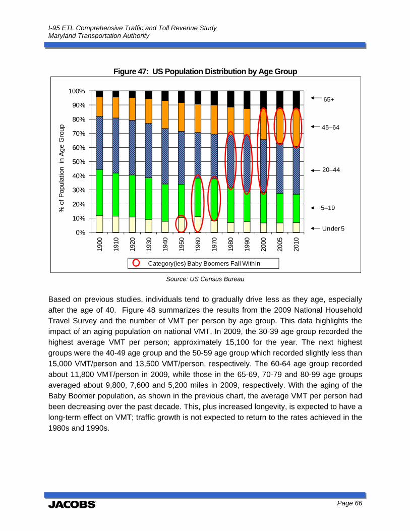
I-95 ETL Comprehensive Traffic and Toll Revenue Study Maryland Transportation Authority
Page 66
Figure 47: US Population Distribution by Age Group
Source: US Census Bureau
Based on previous studies, individuals tend to gradually drive less as they age, especially after the age of 40. Figure 48 summarizes the results from the 2009 National Household Travel Survey and the number of VMT per person by age group. This data highlights the impact of an aging population on national VMT. In 2009, the 30-39 age group recorded the highest average VMT per person; approximately 15,100 for the year. The next highest groups were the 40-49 age group and the 50-59 age group which recorded slightly less than 15,000 VMT/person and 13,500 VMT/person, respectively. The 60-64 age group recorded about 11,800 VMT/person in 2009, while those in the 65-69, 70-79 and 80-99 age groups averaged about 9,800, 7,600 and 5,200 miles in 2009, respectively. With the aging of the Baby Boomer population, as shown in the previous chart, the average VMT per person had been decreasing over the past decade. This, plus increased longevity, is expected to have a long-term effect on VMT; traffic growth is not expected to return to the rates achieved in the 1980s and 1990s.
Under 5
5–19
20–44
45–64
65+
0%
10%
20%
30%
40%
50%
60%
70%
80%
90%
100%19
00
1910
1920
1930
1940
1950
1960
1970
1980
1990
2000
2005
2010
% o
f P
opul
atio
n in
Ag
e G
roup
Category(ies) Baby Boomers Fall Within
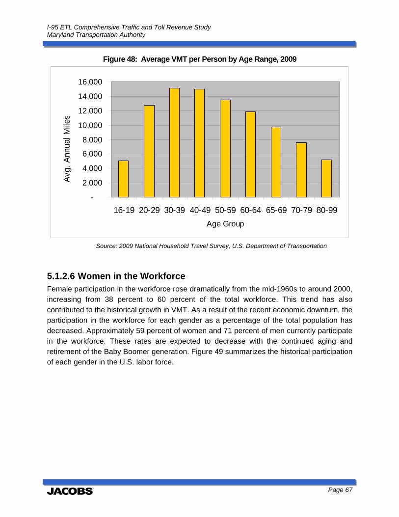
I-95 ETL Comprehensive Traffic and Toll Revenue Study Maryland Transportation Authority
Page 67
Figure 48: Average VMT per Person by Age Range, 2009
Source: 2009 National Household Travel Survey, U.S. Department of Transportation
5.1.2.6 Women in the Workforce Female participation in the workforce rose dramatically from the mid-1960s to around 2000, increasing from 38 percent to 60 percent of the total workforce. This trend has also contributed to the historical growth in VMT. As a result of the recent economic downturn, the participation in the workforce for each gender as a percentage of the total population has decreased. Approximately 59 percent of women and 71 percent of men currently participate in the workforce. These rates are expected to decrease with the continued aging and retirement of the Baby Boomer generation. Figure 49 summarizes the historical participation of each gender in the U.S. labor force.
-
2,000
4,000
6,000
8,000
10,000
12,000
14,000
16,000
16-19 20-29 30-39 40-49 50-59 60-64 65-69 70-79 80-99
Age Group
Avg
. A
nnua
l Mile
s
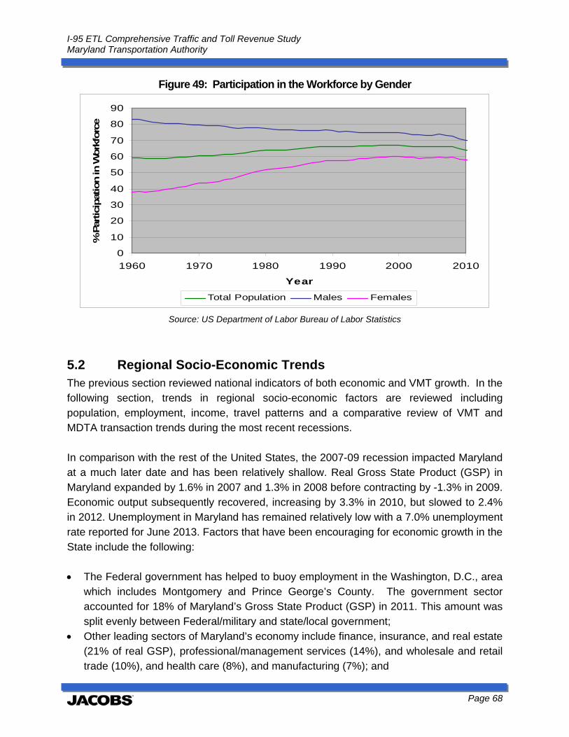
I-95 ETL Comprehensive Traffic and Toll Revenue Study Maryland Transportation Authority
Page 68
Figure 49: Participation in the Workforce by Gender
Source: US Department of Labor Bureau of Labor Statistics
5.2 Regional Socio-Economic Trends The previous section reviewed national indicators of both economic and VMT growth. In the following section, trends in regional socio-economic factors are reviewed including population, employment, income, travel patterns and a comparative review of VMT and MDTA transaction trends during the most recent recessions. In comparison with the rest of the United States, the 2007-09 recession impacted Maryland at a much later date and has been relatively shallow. Real Gross State Product (GSP) in Maryland expanded by 1.6% in 2007 and 1.3% in 2008 before contracting by -1.3% in 2009. Economic output subsequently recovered, increasing by 3.3% in 2010, but slowed to 2.4% in 2012. Unemployment in Maryland has remained relatively low with a 7.0% unemployment rate reported for June 2013. Factors that have been encouraging for economic growth in the State include the following: The Federal government has helped to buoy employment in the Washington, D.C., area
which includes Montgomery and Prince George’s County. The government sector accounted for 18% of Maryland’s Gross State Product (GSP) in 2011. This amount was split evenly between Federal/military and state/local government;
Other leading sectors of Maryland’s economy include finance, insurance, and real estate (21% of real GSP), professional/management services (14%), and wholesale and retail trade (10%), and health care (8%), and manufacturing (7%); and
0
10
20
30
40
50
60
70
80
90
1960 1970 1980 1990 2000 2010
Year
% P
artic
ipation in W
ork
forc
e
Total Population Males Females
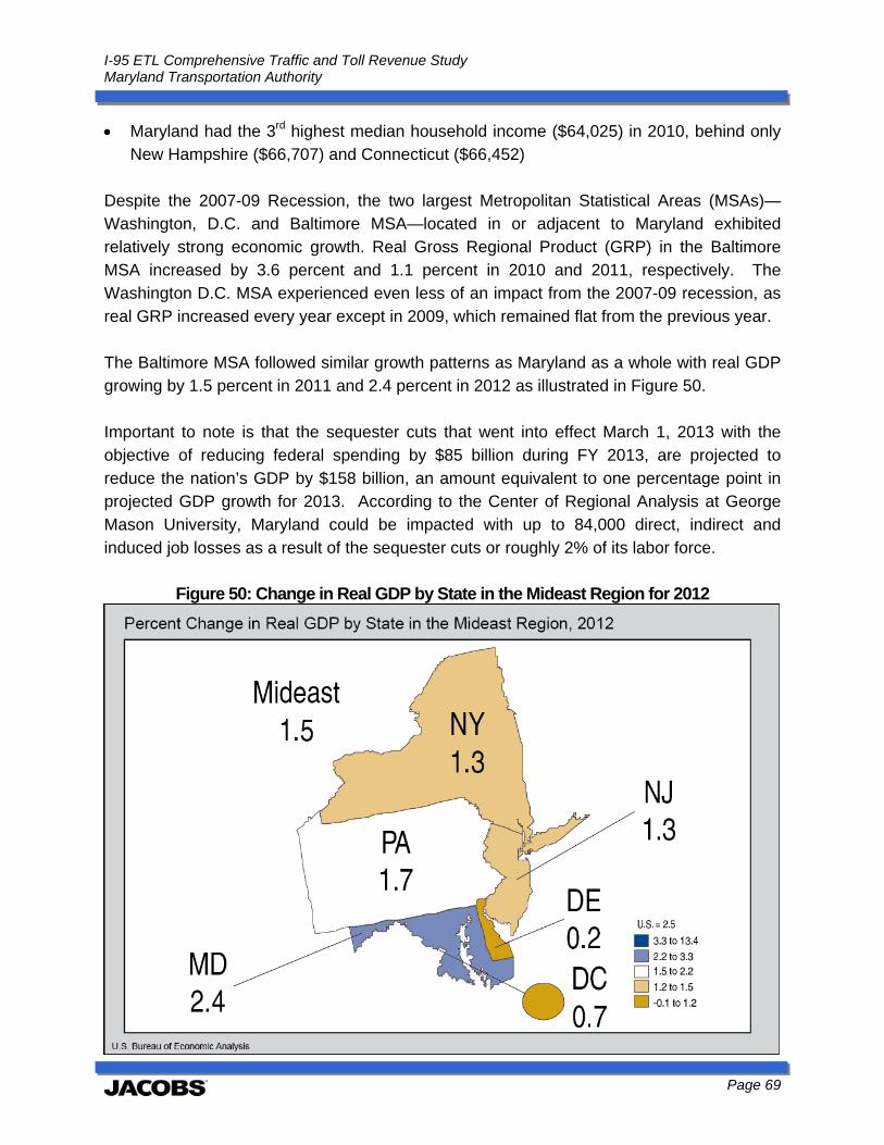
I-95 ETL Comprehensive Traffic and Toll Revenue Study Maryland Transportation Authority
Page 69
Maryland had the 3rd highest median household income ($64,025) in 2010, behind only New Hampshire ($66,707) and Connecticut ($66,452)
Despite the 2007-09 Recession, the two largest Metropolitan Statistical Areas (MSAs)—Washington, D.C. and Baltimore MSA—located in or adjacent to Maryland exhibited relatively strong economic growth. Real Gross Regional Product (GRP) in the Baltimore MSA increased by 3.6 percent and 1.1 percent in 2010 and 2011, respectively. The Washington D.C. MSA experienced even less of an impact from the 2007-09 recession, as real GRP increased every year except in 2009, which remained flat from the previous year. The Baltimore MSA followed similar growth patterns as Maryland as a whole with real GDP growing by 1.5 percent in 2011 and 2.4 percent in 2012 as illustrated in Figure 50. Important to note is that the sequester cuts that went into effect March 1, 2013 with the objective of reducing federal spending by $85 billion during FY 2013, are projected to reduce the nation’s GDP by $158 billion, an amount equivalent to one percentage point in projected GDP growth for 2013. According to the Center of Regional Analysis at George Mason University, Maryland could be impacted with up to 84,000 direct, indirect and induced job losses as a result of the sequester cuts or roughly 2% of its labor force.
Figure 50: Change in Real GDP by State in the Mideast Region for 2012
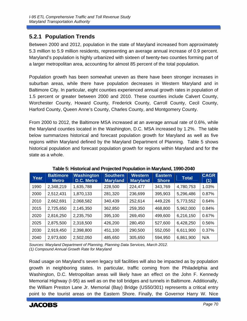
I-95 ETL Comprehensive Traffic and Toll Revenue Study Maryland Transportation Authority
Page 70
5.2.1 Population Trends Between 2000 and 2012, population in the state of Maryland increased from approximately 5.3 million to 5.9 million residents, representing an average annual increase of 0.9 percent. Maryland’s population is highly urbanized with sixteen of twenty-two counties forming part of a larger metropolitan area, accounting for almost 85 percent of the total population. Population growth has been somewhat uneven as there have been stronger increases in suburban areas, while there have population decreases in Western Maryland and in Baltimore City. In particular, eight counties experienced annual growth rates in population of 1.5 percent or greater between 2000 and 2010. These counties include Calvert County, Worchester County, Howard County, Frederick County, Carroll County, Cecil County, Harford County, Queen Anne’s County, Charles County, and Montgomery County. From 2000 to 2012, the Baltimore MSA increased at an average annual rate of 0.6%, while the Maryland counties located in the Washington, D.C. MSA increased by 1.2%. The table below summarizes historical and forecast population growth for Maryland as well as five regions within Maryland defined by the Maryland Department of Planning. Table 5 shows historical population and forecast population growth for regions within Maryland and for the state as a whole.
Table 5: Historical and Projected Population in Maryland, 1990-2040
Year Baltimore
Metro Washington D.C. Metro
Southern Maryland
Western Maryland
Eastern Shore
Total CAGR
(1) 1990 2,348,219 1,635,788 228,500 224,477 343,769 4,780,753 1.03%
2000 2,512,431 1,870,133 281,320 236,699 395,903 5,296,486 0.87%
2010 2,662,691 2,068,582 340,439 252,614 449,226 5,773,552 0.64%
2015 2,725,650 2,145,350 362,850 259,350 468,800 5,962,000 0.84%
2020 2,816,250 2,235,750 395,100 269,450 499,600 6,216,150 0.67%
2025 2,875,500 2,318,500 426,200 280,450 527,600 6,428,250 0.56%
2030 2,919,450 2,398,800 451,100 290,500 552,050 6,611,900 0.37%
2040 2,973,600 2,502,050 485,650 305,650 594,950 6,861,900 N/A
Sources: Maryland Department of Planning, Planning Data Services, March 2012. (1) Compound Annual Growth Rate for Maryland
Road usage on Maryland’s seven legacy toll facilities will also be impacted as by population growth in neighboring states. In particular, traffic coming from the Philadelphia and Washington, D.C. Metropolitan areas will likely have an effect on the John F. Kennedy Memorial Highway (I-95) as well as on the toll bridges and tunnels in Baltimore. Additionally, the William Preston Lane Jr. Memorial (Bay) Bridge (US50/301) represents a critical entry point to the tourist areas on the Eastern Shore. Finally, the Governor Harry W. Nice
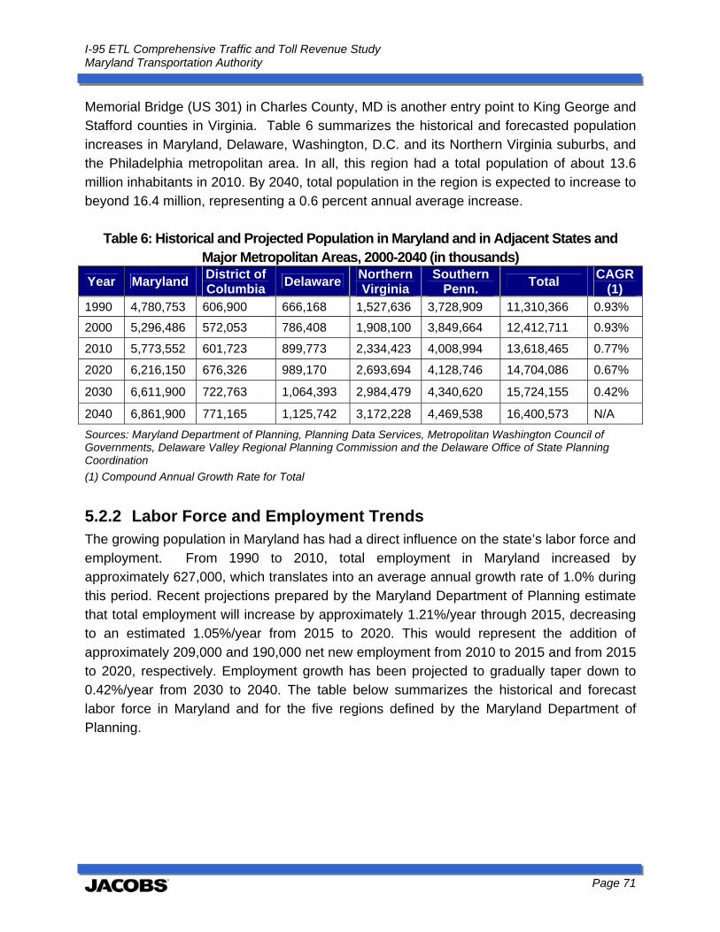
I-95 ETL Comprehensive Traffic and Toll Revenue Study Maryland Transportation Authority
Page 71
Memorial Bridge (US 301) in Charles County, MD is another entry point to King George and Stafford counties in Virginia. Table 6 summarizes the historical and forecasted population increases in Maryland, Delaware, Washington, D.C. and its Northern Virginia suburbs, and the Philadelphia metropolitan area. In all, this region had a total population of about 13.6 million inhabitants in 2010. By 2040, total population in the region is expected to increase to beyond 16.4 million, representing a 0.6 percent annual average increase.
Table 6: Historical and Projected Population in Maryland and in Adjacent States and Major Metropolitan Areas, 2000-2040 (in thousands)
Year Maryland District of Columbia
Delaware Northern Virginia
Southern Penn.
Total CAGR
(1) 1990 4,780,753 606,900 666,168 1,527,636 3,728,909 11,310,366 0.93%
2000 5,296,486 572,053 786,408 1,908,100 3,849,664 12,412,711 0.93%
2010 5,773,552 601,723 899,773 2,334,423 4,008,994 13,618,465 0.77%
2020 6,216,150 676,326 989,170 2,693,694 4,128,746 14,704,086 0.67%
2030 6,611,900 722,763 1,064,393 2,984,479 4,340,620 15,724,155 0.42%
2040 6,861,900 771,165 1,125,742 3,172,228 4,469,538 16,400,573 N/A
Sources: Maryland Department of Planning, Planning Data Services, Metropolitan Washington Council of Governments, Delaware Valley Regional Planning Commission and the Delaware Office of State Planning Coordination
(1) Compound Annual Growth Rate for Total
5.2.2 Labor Force and Employment Trends The growing population in Maryland has had a direct influence on the state’s labor force and employment. From 1990 to 2010, total employment in Maryland increased by approximately 627,000, which translates into an average annual growth rate of 1.0% during this period. Recent projections prepared by the Maryland Department of Planning estimate that total employment will increase by approximately 1.21%/year through 2015, decreasing to an estimated 1.05%/year from 2015 to 2020. This would represent the addition of approximately 209,000 and 190,000 net new employment from 2010 to 2015 and from 2015 to 2020, respectively. Employment growth has been projected to gradually taper down to 0.42%/year from 2030 to 2040. The table below summarizes the historical and forecast labor force in Maryland and for the five regions defined by the Maryland Department of Planning.

I-95 ETL Comprehensive Traffic and Toll Revenue Study Maryland Transportation Authority
Page 72
Table 7: Historical and Projected Potential Labor Force in Maryland, by Region
1990-2040
Year Baltimore Washington,
DC SuburbsSouthern Maryland
Western Maryland
Eastern Shore Total
CAGR (1)Metro
1990 1,781,317 1,379,195 177,903 147,933 250,482 3,736,830
2000 1,905,321 1,498,033 221,824 163,115 297,649 4,085,942 0.93%
2010 2,078,308 1,721,433 269,777 179,392 335,201 4,584,110 1.22%
2015 2,143,414 1,790,484 290,331 186,445 351,226 4,761,900 0.78%
2020 2,220,791 1,871,288 317,799 196,091 375,431 4,981,400 0.92%
2025 2,270,995 1,947,662 343,693 206,582 397,667 5,166,600 0.74%
2030 2,311,337 2,019,135 363,870 215,974 417,513 5,327,830 0.62%
2035 2,346,337 2,069,858 379,046 223,439 435,990 5,454,670 0.48%
2040 2,375,319 2,102,102 393,592 229,895 454,652 5,555,560 0.37%
Source: Maryland Department of Planning, Planning Data Services, March 2012
(1) Compound Annual Growth Rate for Maryland From 2000 to 2005, it is estimated that almost 250,000 net new jobs were created in Maryland; a growth of 1.6 percent per year. Employment growth has been fairly strong across most regions in the state. This strong growth was tempered from 2005 to 2010, with an estimated addition of only 50,000 net new jobs. Table 8 summarizes the total number of full- and part-time jobs in the five Maryland regions. With the end of the recession, employment is forecasted to return to previous growth rates of between one and two percent per year depending on the region. Over the longer term, growth rates are expected to slow slightly as the employment markets become more saturated.
Table 8: Number of Total Jobs by Maryland Region, 1990-2025
Year Baltimore
Metro Washington, DC Suburbs
Southern Maryland
Western Maryland
Eastern Shore
Maryland Maryland
CAGR (1)
1990 1,391,299 957,334 92,345 116,821 179,450 2,737,249 2000 1,514,491 1,087,993 124,138 130,198 208,382 3,065,202 1.14% 2005 1,608,651 1,182,606 146,974 137,353 233,192 3,308,776 1.54% 2010 1,638,800 1,196,800 157,000 135,900 231,300 3,359,800 0.31% 2015 1,742,800 1,280,400 172,600 141,600 251,900 3,589,300 1.33% 2020 1,826,800 1,350,500 185,500 147,000 268,400 3,778,200 1.03% 2025 1,873,700 1,388,800 195,300 151,100 277,900 3,886,800 0.57%
Source: Maryland Department of Planning, Planning Data Services, May 2011
(1) Compound Annual Growth Rate for Maryland

I-95 ETL Comprehensive Traffic and Toll Revenue Study Maryland Transportation Authority
Page 73
Between 2000 and 2010, employment growth in Maryland has been extremely strong in the education and health services, professional services, government, technology, and tourism industries. The Maryland Department of Business and Economic Development has forecasted that employment in these sectors will continue to remain strong in the short- term. According to the 2010 Census, Maryland had the second highest percentage (26.1 percent) of professional and technical workers as a percentage of the total employment. In particular, the technology sector currently employs an estimated 87 out of every 1,000 private sector workers, ranking 4th in the United States. Additionally, employment in the construction and natural resources sector increased 2% from 2011 to 2012. Similar to other regions in the U.S., the manufacturing sector has experienced a reduction in total employment in recent years. The table below summarizes the 15 largest employers in Maryland during 2011.
Table 9: Largest 25 Employers in State of Maryland, 2011
Employer Employment Industry Fort George G. Meade 44,540 Military installation/intelligence University System of Maryland 36,380 Higher education Johns Hopkins University 27,000 Higher education Johns Hopkins Hospital & Health System
20,100 Hospitals; health services
National Institutes of Health 18,800 Federal agency Walmart 17,420 Consumer goods Aberdeen Proving Ground 15,580 Military installation
University of Maryland Medical System
15,000 Hospitals; health services
MedStar Health 14,600 Hospitals; health services Giant Food 13,260 Groceries U.S. Social Security Administration
13,000 Federal agency
Walter Reed National Military Medical Center
11,000 Hospital; health services
Northrop Grumman 10,980 Electronic systems Naval Air Station Patuxent River
10,960 Military installation
Marriott International 10,000 Food and lodging services Source: Maryland Department of Business and Economic Development, 2010
While tracking national trends, unemployment in Maryland has remained below that of the U.S. Unemployment increased during the 2001 recession and during 2007-09 recession. Unemployment is not uniform across the state as the unemployment rate in the Washington, D.C. MSA was 6.0%, but 7.9% in the Baltimore MSA, as of June 2013. Figure 22 summarizes regional, state, and national unemployment rates tracked by the Bureau of Labor Statistics (BLS) from 1998 to June 2013.
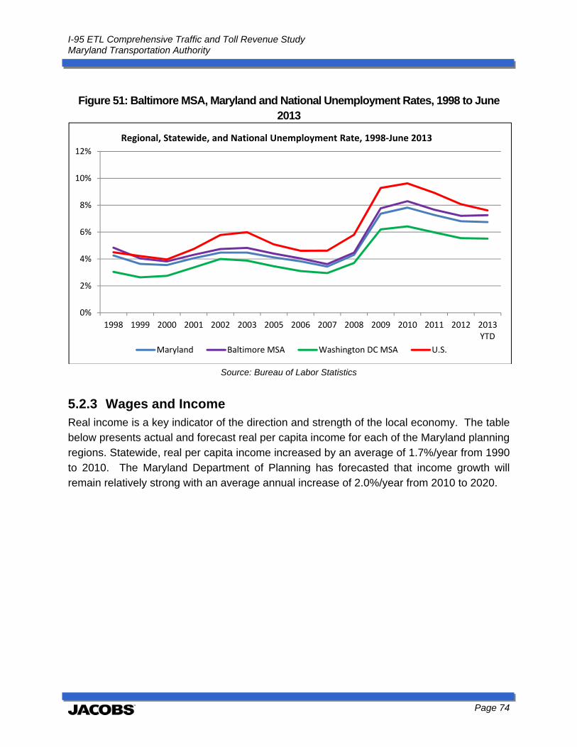
I-95 ETL Comprehensive Traffic and Toll Revenue Study Maryland Transportation Authority
Page 74
Figure 51: Baltimore MSA, Maryland and National Unemployment Rates, 1998 to June
2013
Source: Bureau of Labor Statistics
5.2.3 Wages and Income Real income is a key indicator of the direction and strength of the local economy. The table below presents actual and forecast real per capita income for each of the Maryland planning regions. Statewide, real per capita income increased by an average of 1.7%/year from 1990 to 2010. The Maryland Department of Planning has forecasted that income growth will remain relatively strong with an average annual increase of 2.0%/year from 2010 to 2020.
0%
2%
4%
6%
8%
10%
12%
1998 1999 2000 2001 2002 2003 2005 2006 2007 2008 2009 2010 2011 2012 2013YTD
Maryland Baltimore MSA Washington DC MSA U.S.
Regional, Statewide, and National Unemployment Rate, 1998‐June 2013
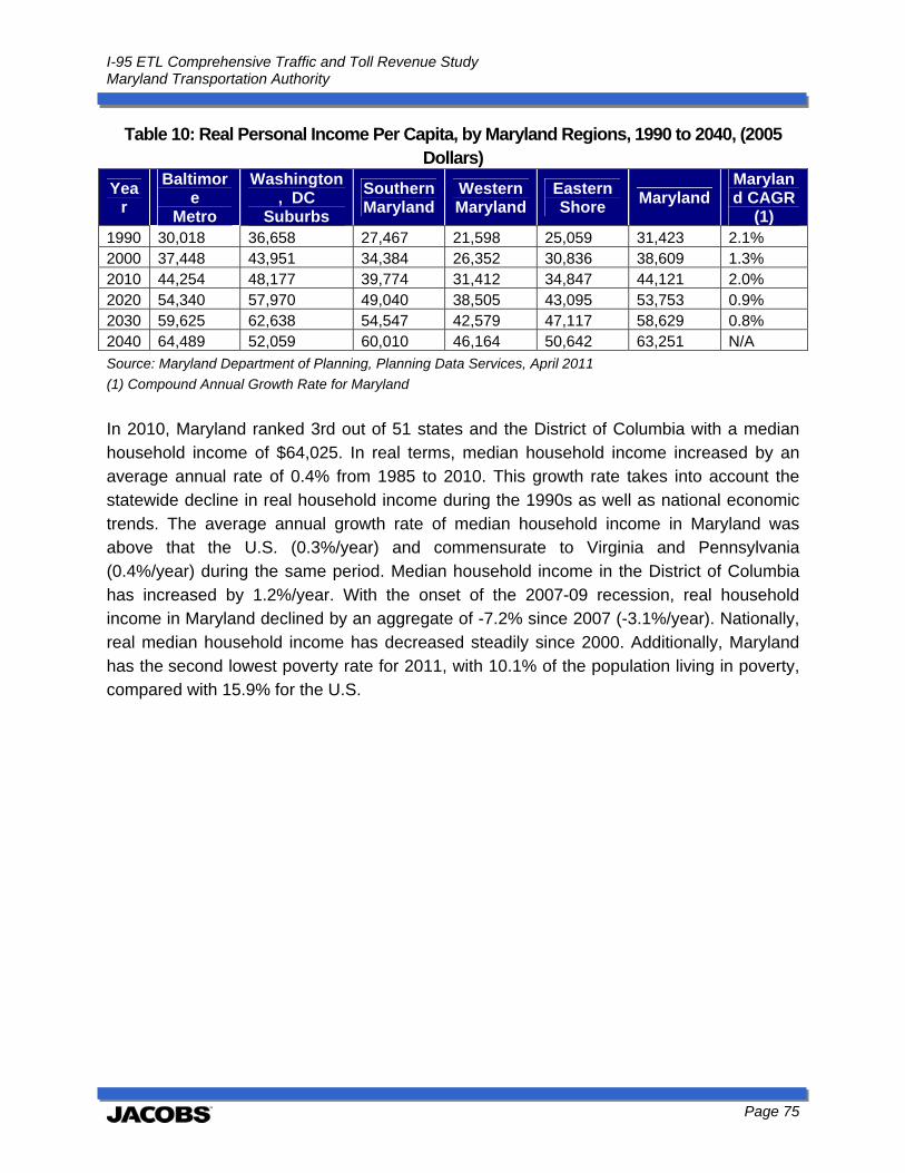
I-95 ETL Comprehensive Traffic and Toll Revenue Study Maryland Transportation Authority
Page 75
Table 10: Real Personal Income Per Capita, by Maryland Regions, 1990 to 2040, (2005 Dollars)
Year
Baltimore
Metro
Washington, DC
Suburbs
Southern Maryland
Western Maryland
Eastern Shore
Maryland Maryland CAGR
(1) 1990 30,018 36,658 27,467 21,598 25,059 31,423 2.1% 2000 37,448 43,951 34,384 26,352 30,836 38,609 1.3% 2010 44,254 48,177 39,774 31,412 34,847 44,121 2.0% 2020 54,340 57,970 49,040 38,505 43,095 53,753 0.9% 2030 59,625 62,638 54,547 42,579 47,117 58,629 0.8% 2040 64,489 52,059 60,010 46,164 50,642 63,251 N/A Source: Maryland Department of Planning, Planning Data Services, April 2011
(1) Compound Annual Growth Rate for Maryland
In 2010, Maryland ranked 3rd out of 51 states and the District of Columbia with a median household income of $64,025. In real terms, median household income increased by an average annual rate of 0.4% from 1985 to 2010. This growth rate takes into account the statewide decline in real household income during the 1990s as well as national economic trends. The average annual growth rate of median household income in Maryland was above that the U.S. (0.3%/year) and commensurate to Virginia and Pennsylvania (0.4%/year) during the same period. Median household income in the District of Columbia has increased by 1.2%/year. With the onset of the 2007-09 recession, real household income in Maryland declined by an aggregate of -7.2% since 2007 (-3.1%/year). Nationally, real median household income has decreased steadily since 2000. Additionally, Maryland has the second lowest poverty rate for 2011, with 10.1% of the population living in poverty, compared with 15.9% for the U.S.
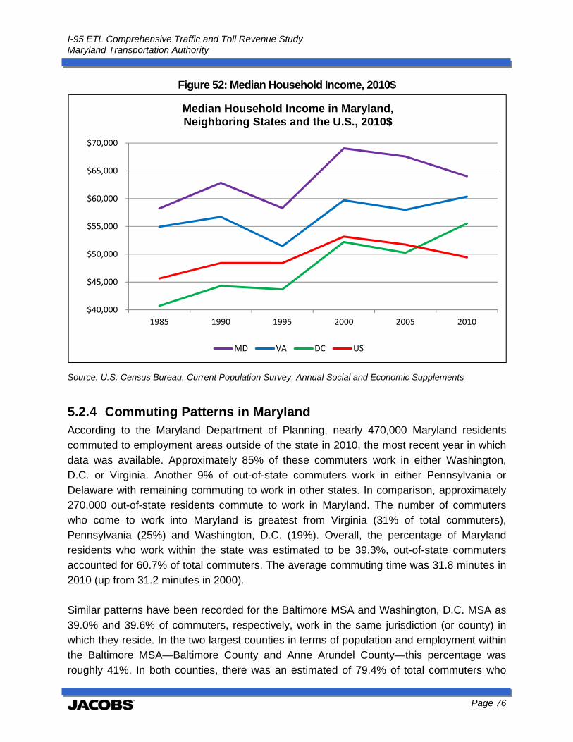
I-95 ETL Comprehensive Traffic and Toll Revenue Study Maryland Transportation Authority
Page 76
Figure 52: Median Household Income, 2010$
Source: U.S. Census Bureau, Current Population Survey, Annual Social and Economic Supplements
5.2.4 Commuting Patterns in Maryland According to the Maryland Department of Planning, nearly 470,000 Maryland residents commuted to employment areas outside of the state in 2010, the most recent year in which data was available. Approximately 85% of these commuters work in either Washington, D.C. or Virginia. Another 9% of out-of-state commuters work in either Pennsylvania or Delaware with remaining commuting to work in other states. In comparison, approximately 270,000 out-of-state residents commute to work in Maryland. The number of commuters who come to work into Maryland is greatest from Virginia (31% of total commuters), Pennsylvania (25%) and Washington, D.C. (19%). Overall, the percentage of Maryland residents who work within the state was estimated to be 39.3%, out-of-state commuters accounted for 60.7% of total commuters. The average commuting time was 31.8 minutes in 2010 (up from 31.2 minutes in 2000). Similar patterns have been recorded for the Baltimore MSA and Washington, D.C. MSA as 39.0% and 39.6% of commuters, respectively, work in the same jurisdiction (or county) in which they reside. In the two largest counties in terms of population and employment within the Baltimore MSA—Baltimore County and Anne Arundel County—this percentage was roughly 41%. In both counties, there was an estimated of 79.4% of total commuters who
$40,000
$45,000
$50,000
$55,000
$60,000
$65,000
$70,000
1985 1990 1995 2000 2005 2010
MD VA DC US
Median Household Income in Maryland, Neighboring States and the U.S., 2010$
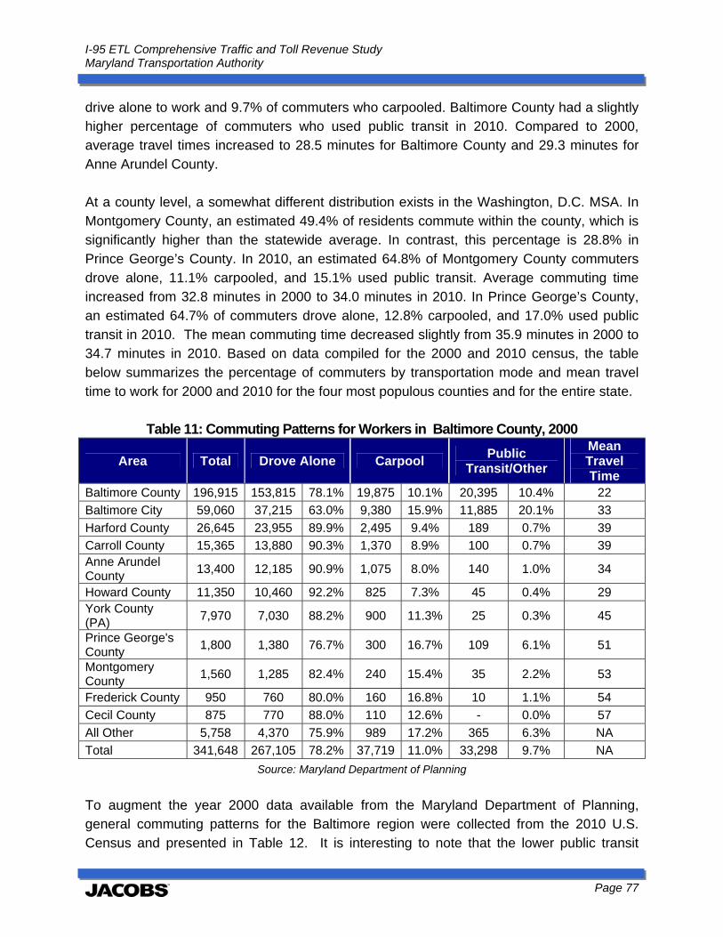
I-95 ETL Comprehensive Traffic and Toll Revenue Study Maryland Transportation Authority
Page 77
drive alone to work and 9.7% of commuters who carpooled. Baltimore County had a slightly higher percentage of commuters who used public transit in 2010. Compared to 2000, average travel times increased to 28.5 minutes for Baltimore County and 29.3 minutes for Anne Arundel County. At a county level, a somewhat different distribution exists in the Washington, D.C. MSA. In Montgomery County, an estimated 49.4% of residents commute within the county, which is significantly higher than the statewide average. In contrast, this percentage is 28.8% in Prince George’s County. In 2010, an estimated 64.8% of Montgomery County commuters drove alone, 11.1% carpooled, and 15.1% used public transit. Average commuting time increased from 32.8 minutes in 2000 to 34.0 minutes in 2010. In Prince George’s County, an estimated 64.7% of commuters drove alone, 12.8% carpooled, and 17.0% used public transit in 2010. The mean commuting time decreased slightly from 35.9 minutes in 2000 to 34.7 minutes in 2010. Based on data compiled for the 2000 and 2010 census, the table below summarizes the percentage of commuters by transportation mode and mean travel time to work for 2000 and 2010 for the four most populous counties and for the entire state.
Table 11: Commuting Patterns for Workers in Baltimore County, 2000
Area Total Drove Alone Carpool Public
Transit/Other
Mean Travel Time
Baltimore County 196,915 153,815 78.1% 19,875 10.1% 20,395 10.4% 22
Baltimore City 59,060 37,215 63.0% 9,380 15.9% 11,885 20.1% 33
Harford County 26,645 23,955 89.9% 2,495 9.4% 189 0.7% 39
Carroll County 15,365 13,880 90.3% 1,370 8.9% 100 0.7% 39 Anne Arundel County
13,400 12,185 90.9% 1,075 8.0% 140 1.0% 34
Howard County 11,350 10,460 92.2% 825 7.3% 45 0.4% 29 York County (PA)
7,970 7,030 88.2% 900 11.3% 25 0.3% 45
Prince George's County
1,800 1,380 76.7% 300 16.7% 109 6.1% 51
Montgomery County
1,560 1,285 82.4% 240 15.4% 35 2.2% 53
Frederick County 950 760 80.0% 160 16.8% 10 1.1% 54
Cecil County 875 770 88.0% 110 12.6% - 0.0% 57
All Other 5,758 4,370 75.9% 989 17.2% 365 6.3% NA
Total 341,648 267,105 78.2% 37,719 11.0% 33,298 9.7% NA
Source: Maryland Department of Planning
To augment the year 2000 data available from the Maryland Department of Planning, general commuting patterns for the Baltimore region were collected from the 2010 U.S. Census and presented in Table 12. It is interesting to note that the lower public transit

I-95 ETL Comprehensive Traffic and Toll Revenue Study Maryland Transportation Authority
Page 78
percentages of the suburban communities of Baltimore are supplemented by increased percentage of people working from home. This is less demonstrated in the counties that are suburban to Washington D.C.
Table 12: Commuting Patterns in Baltimore Region
Area Drive Alone Carpool
Public Transit
Work From Home Other
Baltimore County 79.4% 9.7% 4.3% 3.5% 3.1%
Baltimore City 60.0% 11.4% 17.6% 2.6% 8.4%
Harford County 84.0% 8.8% 0.9% 4.4% 1.9%
Carroll County 82.8% 8.2% 0.7% 5.7% 2.6%
Anne Arundel County 79.4% 9.7% 3.2% 5.0% 2.7%
Howard County 80.9% 7.6% 3.7% 5.5% 2.3%
Prince George's County 64.7% 12.8% 17.0% 2.9% 2.6%
Montgomery County 64.8% 11.1% 15.1% 5.9% 3.1% Frederick County 74.6% 12.2% 3.7% 5.4% 4.1%
Cecil County 80.7% 11.2% 1.1% 4.6% 2.4%
Total 71.8% 10.7% 9.8% 4.3% 3.4%
5.2.5 Statewide Economic Forecast Economic growth and employment in Maryland has historically followed national trends, but overall economic conditions have tended to be stronger due to the large number of professional employees, the state’s close proximity to the Federal government offices in Washington, D.C., and relatively high median house income. Additionally, the value of exports transported through the Port of Baltimore has increased by 135% from 2006 to 2011. These strengths also represent potential vulnerabilities. Proposed reductions in federal spending in 2013, particularly in the defense industry, could impact Maryland more deeply relative to other states. Moreover, a potential slowdown in global economic conditions would lead to a decrease in exports, particularly to China and Europe. Absent these uncertainties, Maryland economy is expected to grow at a relatively healthy rate. An economic forecast prepared by Chase and JP Morgan in early 2013 forecasted that
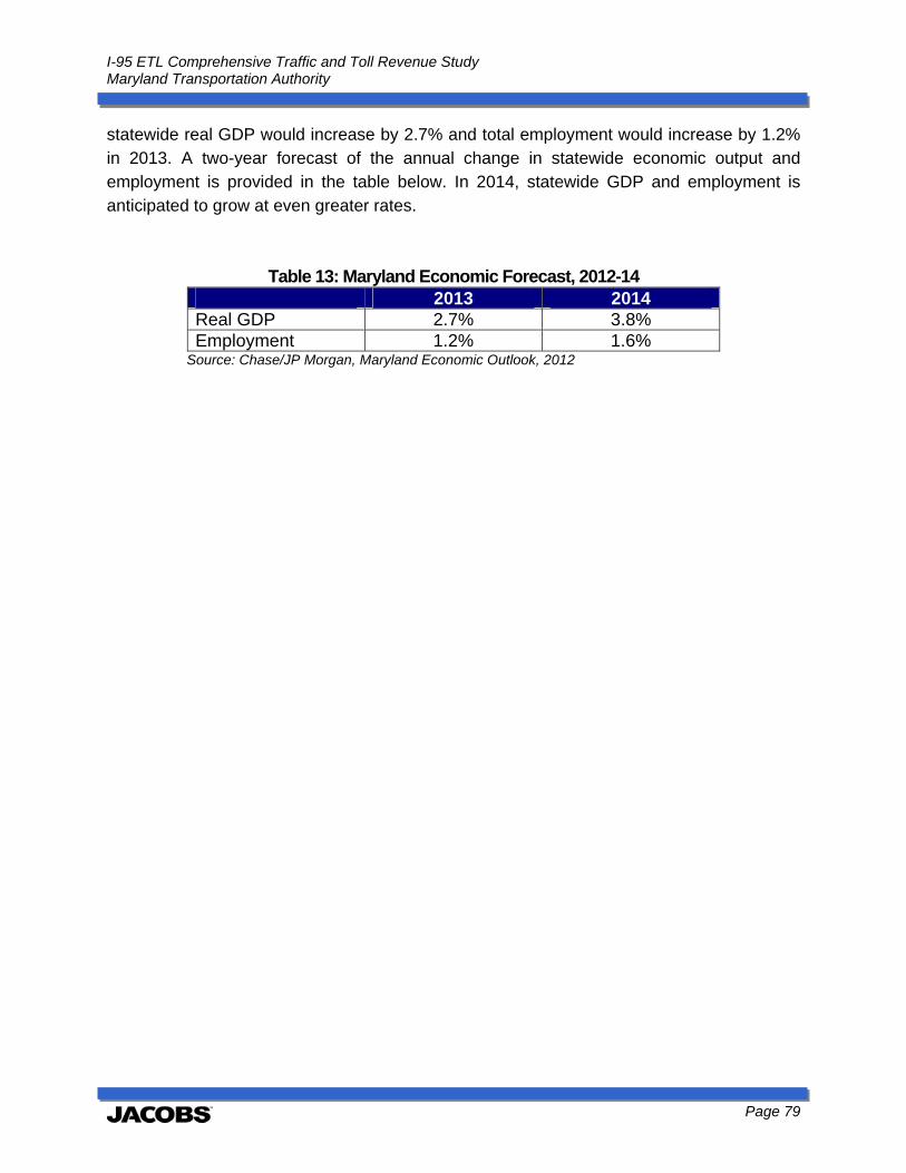
I-95 ETL Comprehensive Traffic and Toll Revenue Study Maryland Transportation Authority
Page 79
statewide real GDP would increase by 2.7% and total employment would increase by 1.2% in 2013. A two-year forecast of the annual change in statewide economic output and employment is provided in the table below. In 2014, statewide GDP and employment is anticipated to grow at even greater rates.
Table 13: Maryland Economic Forecast, 2012-14 2013 2014
Real GDP 2.7% 3.8% Employment 1.2% 1.6%
Source: Chase/JP Morgan, Maryland Economic Outlook, 2012
I-95 ETL Comprehensive Traffic and Toll Revenue Study Maryland Transportation Authority
Page 80
6.0 Traffic and Toll Revenue Modeling and Estimates In this section, the traffic and toll revenue modeling methodology, assumptions and estimates are presented. First, the methodology of the traffic, toll schedule and toll revenue modeling is reviewed including the use of the Baltimore Metropolitan Council travel demand model (BMC Model), the I-95 ETL VISSIM microsimulation model (VISSIM Model) and development of the I-95 ETL traffic, toll schedule and toll revenue forecasting model (T&R Model). The basic assumptions used for the analysis include those controlled by the MDTA such as I-95 ETL limits, access points and tolling points and tolling policy as well as those determined by motorists including corridor demand, hourly traffic profiles, values of time, payment and vehicle class mixes and other consumer-driven assumptions that lay outside of the control of the toll facility operator. The forecasts of toll schedule, tolled traffic and toll revenue are presented for the multiple cases run. The base case assumes the toll policy presented in the assumptions portion of this section. The maximum throughput case provides maximum traffic flow through the corridor constrained only by minimum toll considerations on the ETL. The maximizing revenue case provides estimates assuming the operator would like to maximize toll revenue for the corridor without consideration to traffic flow outside of when it affects revenue potential. The final step in the forecasting process is the conduct of risk analysis. The risk analysis allows for the base case traffic and toll revenue forecasts to be placed within the range of all potential forecast outcomes for the I-95 ETL providing a comfort level regarding the probability of attaining forecasted revenues.
6.1 Modeling Methodology The forecasting of traffic, toll schedules, and toll revenue for managed lane facilities requires the use of multiple forecasting models on multiple modeling platforms. This includes the Baltimore Metropolitan Council travel demand model (BMC Model), the I-95 ETL VISSIM micro-simulation model (VISSIM model) and the I-95 ETL traffic, toll schedule and toll revenue forecasting model (T&R Model). Figure 53 presents the general work flow for the forecasting effort with each model separated by color coding. The first step is the use of the BMC model to provide forecasted average weekday traffic volumes in the corridor for 2015 and 2025 to the T&R model. This data combined with historical traffic data provides forecasted levels of corridor demand for the T&R model. Additionally origin and destination matrices from the BMC model are
I-95 ETL Comprehensive Traffic and Toll Revenue Study Maryland Transportation Authority
Page 81
provided to the VISSIM model to develop an understanding of operational characteristics of the corridor, which also feed into the T&R model. The T&R model then estimates the toll schedule needed to manage traffic in the ETL in half hour increments. This is then subject to an adjustment to the toll schedule to accommodate peak, off-peak and overnight pricing periods by day of the week to be consistent with current MDTA toll policies on the ICC. The T&R model is then re-run with toll schedule as the input and traffic and toll revenue estimates as the output. This output is then provided to the VISSIM model to ensure that traffic can operate efficiently within the corridor based on the estimates of traffic by half hour in the general purpose and ETL for each forecast year. The details of each model, the inputs and outputs, are provided in the following sections.
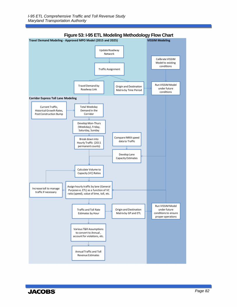
I-95 ETL Comprehensive Traffic and Toll Revenue Study Maryland Transportation Authority
Page 82
Figure 53: I-95 ETL Modeling Methodology Flow Chart
VISSIM ModelingTravel Demand Modeling ‐ Approved MPO Model (2015 and 2025)
Corridor Express Toll Lane Modeling
Traffic Assignment
Travel Demand by Roadway Link
Update Roadway Network
Total Weekday Demand in the
Corridor
Calculate Volume to Capacity (VC) Ratios
Break down into Hourly Traffic (2011permanent counts)
Assign hourly traffic by lane (General Purpose vs. ETL) as a function of VC ratio (speed), value of time, toll, etc.
Current Traffic, HistoricalGrowth Rates, Post Construction Bump
Increase toll to manage traffic if necessary
Traffic and Toll RateEstimates by Hour
Various T&R Assumptions to convert to Annual ,
account for violations, etc.
Annual Traffic and Toll RevenueEstimates
Origin and Destination Matrix by Time Period
Develop Mon‐Thurs(Weekday), Friday, Saturday, Sunday
Develop Lane Capacity Estimates
Compare INRIX speed data to Traffic
Origin and Destination Matrix by GP and ETL
Calibrate VISSIM Model to existing
conditions
Run VISSIM Model under future conditions
Run VISSIM Model under future
conditions to ensure proper operations
I-95 ETL Comprehensive Traffic and Toll Revenue Study Maryland Transportation Authority
Page 83
6.1.1 Travel Demand and Microsimulation Modeling The BMC Travel Demand Model, the regional travel forecasting model and a corridor specific VISSIM model, and a micro-simulation model, were used to provide input into the T&R forecasting model. This section provides an overview of the process and use of these two modeling platforms. More detailed modeling results are provided in Appendix B of this report. The BMC Model provides estimates of travel demand for each major roadway link in the Baltimore region as a function of population and employment centers and estimated trip making characteristics and roadway network capacity to handle travel movements. For this analysis, the model years of 2011 (base year), 2015 and 2025 were used. First, the roadway network in the corridor was reviewed to make sure the model was appropriately coded to model current year conditions. Then the resulting 2011 traffic estimates were compared to actual counts in the corridor to determine the accuracy of the base year calibration in the corridor. The model produced results that were approximately 4.5 percent below actual traffic counts on I-95, considered reasonable for this step in the process. Future year model runs were conducted for 2015 and 2025 with the inclusion of the I-95 ETLs as defined within this document. Those results fed into the T&R forecasting model that is described in the subsequent section as well as the VISSIM model described below. The I-95 ETL VISSIM model is a corridor specific model that dynamically assigns traffic to the I-95 corridor to allow operational analysis to be conducted. The BMC travel demand model provided the needed origin and destination matrices as input to the VISSIM model and various calibration techniques were employed to develop the base year model. Similar to the BMC model, the future roadway network was coded to reflect the proposed infrastructure, namely the I-95 ETLs and access points. The simulation models were run to assure that the ETLs and general purpose lanes would operate effectively, especially at merge points. Additionally, travel times and speeds as a function of volume in the corridor were used as input into the T&R Forecasting Model described in the next section. The VISSIM Model was also run upon completion of the T&R Forecasting Model to assure that the ETLs would operate as estimated from the T&R Forecasting Model. More detail regarding this step in the analysis, including calibration techniques, assignment runs conducted, and results of those assignment runs are provided in Appendix B.
6.1.2 T&R Forecasting Model The T&R Model was developed specifically for the I-95 ETL T&R Study to accommodate the unique aspects of the toll policies tested and the corridor for this project. Two different forecasting models were developed. The first used the basic assumptions of corridor

I-95 ETL Comprehensive Traffic and Toll Revenue Study Maryland Transportation Authority
Page 84
demand by year, day of week, half hour, payment class, vehicle class, origin/destination pair, values of time and lane capacities to determine traffic by half hour for an eleven year period (2015-2025) as well as the toll schedule needed for that same time period to reflect the constraints of the toll plan. These constraints included the use of ICC toll rate ranges for the project and the maintenance of 55 miles per hour on the ETL during all times. The maintenance of speed on the ETL required time of day pricing for some half hour periods. The allocation of vehicles to the ETL in the model is a function of time savings between the toll free general purpose lanes and the tolled ETL. Again, the output of this model is the traffic and toll revenue for the ETL under certain assumptions, but more importantly, the estimated minimum toll schedule needed by half hour by day for the eleven year period to maintain travel speeds of 55 mph in the ETL. The second model developed uses the same basic assumptions of values of time, lane capacities, corridor demand, etc., as presented for the first model, but this model also uses a set time-of-day toll schedule as an input. The reason for the development of this model is to forecast traffic and toll revenue constrained by six tolling periods to accommodate ease of use for the motorists in the corridor and align with current ICC toll policies. Under these sets of assumptions the toll schedule is sized by the first model, thus, ensuring maintenance of travel speeds on the ETL and the traffic allocation is reassigned based upon toll levels in the six tolling periods. This two-step process allows for first, the sizing of the toll schedule to comply with toll policy and the implementation of actual operational toll policy to understand the reaction of traffic to such constraints. Each day of the week was modeled individually to reflect the unique nature of traffic operations by day, most significantly corridor demand, hourly profile and driver behavior. The analysis and modeling did not take into account holiday events such as the Wednesday before Thanksgiving, the Christmas holiday rush period and the like. It is estimated that any inclusion of a holiday peak period toll rate schedule would be marginally beneficial to the overall traffic and toll revenue estimates. Due to the limited benefit, as compared to an entire year of traffic and toll revenue, this analysis was not incorporated into the estimates. The final result of this modeling effort incorporates anticipated ramp-up, violation rates and other assumptions to arrive at estimates of traffic and toll revenue for the ETL for the forecast period. The various assumptions introduced in this section are presented in more detail in the next section.
I-95 ETL Comprehensive Traffic and Toll Revenue Study Maryland Transportation Authority
Page 85
6.2 Assumptions of Analysis In this section, the basic assumptions of the analysis are presented starting with the assumptions that the MDTA controls including the infrastructure that is being built and the toll plan that will be implemented. This is in addition to those assumptions outside of the control of the MDTA such as motorists’ behavior, corridor growth, traffic operational assumptions and the like. The results of variations on the first set of assumptions, those controlled by the MDTA, are presented in subsequent sections of this report defined as alternative analyses. The results of variations on the second set of assumptions, those outside of the control of the MDTA, are presented in the risk analysis section. Figure 54 presents the basic assumptions of the analysis, detailed by those controlled by the MDTA and those outside of the control of the MDTA. Additionally, Figure 55 presents the assumed toll stick diagram for the I-95 ETL project. It is assumed the full project will be opened on December 1, 2014 for the MDTA. For southbound traffic there will be ingress points between MD 43 and E. Joppa Road and from MD 43 and egress points on I-895 to Moravia Road and south of Moravia Road and on I-95 south of Pulaski Highway. The northbound infrastructure will be symmetric to the southbound infrastructure with ingress points on I-895 south of Moravia Road, from Moravia Road and on I-95 south of Pulaski Highway and egress points to MD 43 and between MD 43 and E. Joppa Road. The toll gantry will be between I-695 and the split of I-95 and I-895. There will only be one toll gantry because all trips are of almost the same length. The toll plan, as discussed previously, was determined by the MDTA as a combination of existing toll policies on MDTA facilities and leading trends of managed lane toll policy throughout the United States. The most salient policies to this analysis include the maintenance of speeds on the ETL at 55 miles per hour and adherence to current ICC toll rate ranges as presented in Figure 54. Additionally, the facility will offer collection of tolls through traditional E-ZPass as well as for motorists without E-ZPass via image collection and billing. The toll rates for image-based tolls or video tolls will be 50 percent more than the toll for E-ZPass with a minimum surcharge of $1.00 and a maximum surcharge of $15.00. This policy is consistent with the current operations of the MDTA facilities. Other toll plan assumptions include the use of current axle multipliers for the ICC for the tolling of trucks in the ETL and no standard toll escalation for the lanes over time, only as it relates to the need to raise tolls to maintain travel speeds on the facility. The remaining assumptions, which are beyond the control of the MDTA, are presented in the next section.
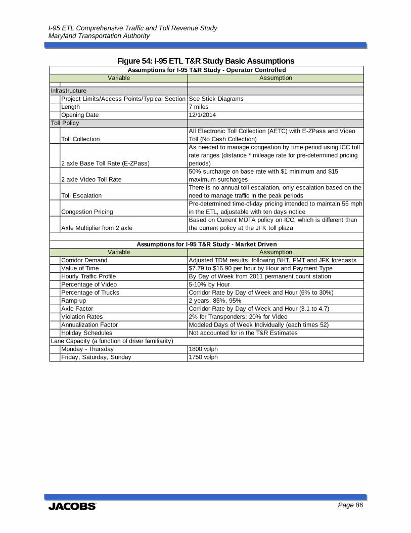
I-95 ETL Comprehensive Traffic and Toll Revenue Study Maryland Transportation Authority
Page 86
Figure 54: I-95 ETL T&R Study Basic Assumptions
Assumption
InfrastructureProject Limits/Access Points/Typical Section See Stick DiagramsLength 7 milesOpening Date 12/1/2014
Toll Policy
Toll CollectionAll Electronic Toll Collection (AETC) with E-ZPass and Video Toll (No Cash Collection)
2 axle Base Toll Rate (E-ZPass)
As needed to manage congestion by time period using ICC toll rate ranges (distance * mileage rate for pre-determined pricing periods)
2 axle Video Toll Rate50% surcharge on base rate with $1 minimum and $15 maximum surcharges
Toll EscalationThere is no annual toll escalation, only escalation based on the need to manage traffic in the peak periods
Congestion PricingPre-determined time-of-day pricing intended to maintain 55 mph in the ETL, adjustable with ten days notice
Axle Multiplier from 2 axleBased on Current MDTA policy on ICC, which is different than the current policy at the JFK toll plaza
AssumptionCorridor Demand Adjusted TDM results, following BHT, FMT and JFK forecastsValue of Time $7.79 to $16.90 per hour by Hour and Payment TypeHourly Traffic Profile By Day of Week from 2011 permanent count stationPercentage of Video 5-10% by HourPercentage of Trucks Corridor Rate by Day of Week and Hour (6% to 30%)Ramp-up 2 years, 85%, 95%Axle Factor Corridor Rate by Day of Week and Hour (3.1 to 4.7)Violation Rates 2% for Transponders; 20% for VideoAnnualization Factor Modeled Days of Week Individually (each times 52)Holiday Schedules Not accounted for in the T&R Estimates
Lane Capacity (a function of driver familiarity)Monday - Thursday 1800 vplphFriday, Saturday, Sunday 1750 vplph
Assumptions for I-95 T&R Study - Operator ControlledVariable
Assumptions for I-95 T&R Study - Market DrivenVariable
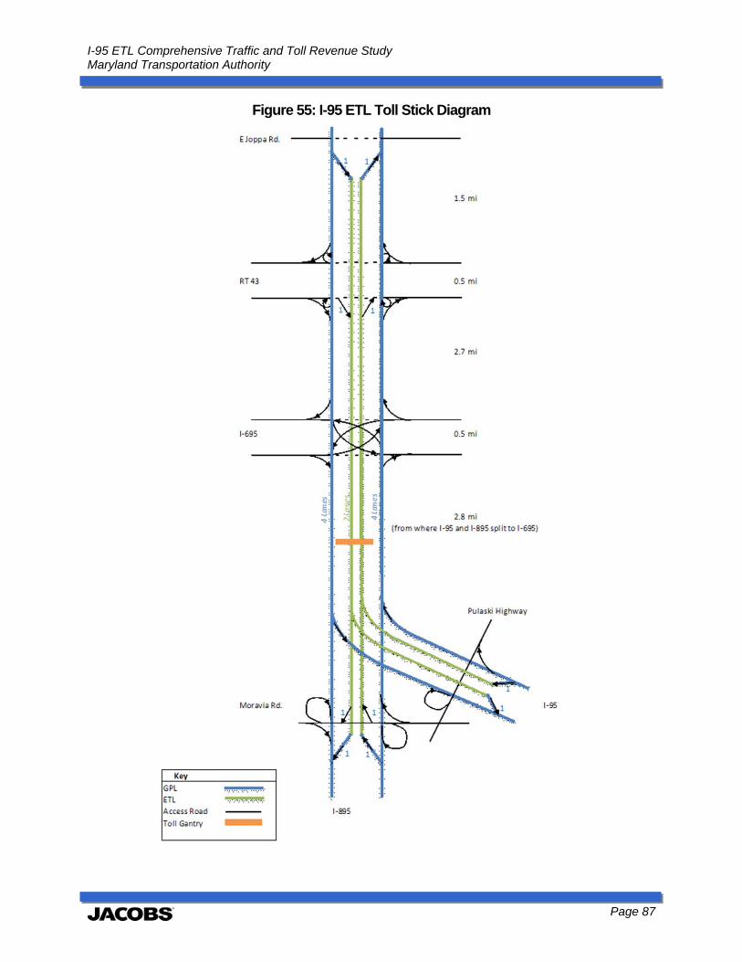
I-95 ETL Comprehensive Traffic and Toll Revenue Study Maryland Transportation Authority
Page 87
Figure 55: I-95 ETL Toll Stick Diagram
I-95 ETL Comprehensive Traffic and Toll Revenue Study Maryland Transportation Authority
Page 88
6.2.1 Traffic and Toll Revenue Assumptions In this section, the assumptions of the analysis that are outside of the control of the MDTA are presented. These assumptions include corridor demand, vehicle/payment composition, motorists’ behavior and traffic operations. These are the major assumptions that are inputs for the T&R forecasting models described previously.
6.2.1.1 Corridor Demand The forecasted corridor demand in the I-95 corridor that is input into the T&R forecasting models is a key driver of traffic and toll revenue in the ETL. As demand in the corridor increases, the attractiveness of the free-flowing ETL increases. This, in-turn, creates the need for congestion pricing during peak hours. The projected corridor demand for this analysis was forecasted using output data from the BMC travel demand model, historical traffic volumes, projected growth in demographics and projected adjustments to trip making in the future. Figure 56 presents historical traffic volumes for the I-95 corridor between I-695 and the split of I-895 and I-95, the approximate location of the ETL toll gantry. The Figure also provides linear regression analysis for various time periods including 1980 to 2000, 1990 to 2000, 1980 to 2012, 1990 to 2012, 2000 to 2012 and 2005 to 2012. That analysis is provided in purple, yellow, red, green, dark blue and orange lines respectively. Linear regression of this data allows for an understanding of potential future year traffic volumes based on historical experience, which is provided in Table 14. In this table, the corridor traffic volumes used for this analysis are also presented to provide a comparison. These estimates remove the induced demand estimated that will be presented later in this section. Notice that generally the estimated future traffic volumes based on data from the 1980s presents quite high future estimates while with the inclusion of more recent data, the estimated future traffic is much lower. The base corridor traffic levels generally fall between the 2005 to 2012 and 2000 to 2012 regression and are very similar to the 1990 to 2012 regression. The estimates are significantly below the earlier data that incorporated 1980 to 2000 growth experience.
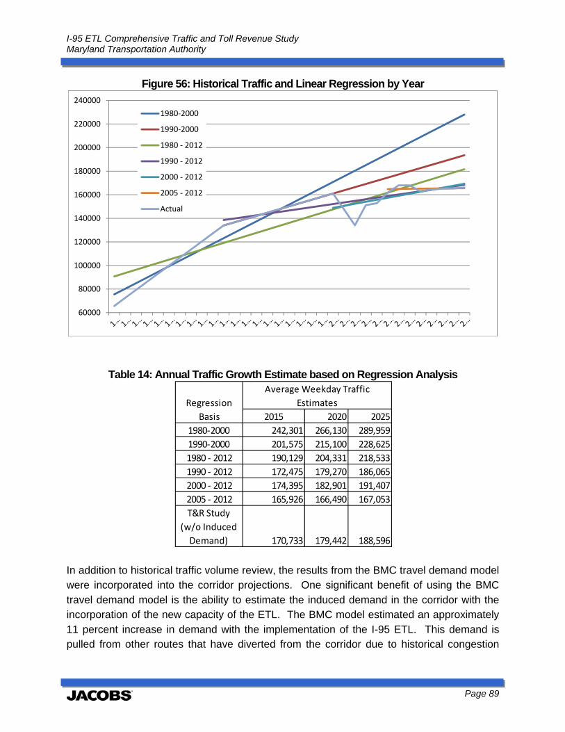
I-95 ETL Comprehensive Traffic and Toll Revenue Study Maryland Transportation Authority
Page 89
Figure 56: Historical Traffic and Linear Regression by Year
Table 14: Annual Traffic Growth Estimate based on Regression Analysis
In addition to historical traffic volume review, the results from the BMC travel demand model were incorporated into the corridor projections. One significant benefit of using the BMC travel demand model is the ability to estimate the induced demand in the corridor with the incorporation of the new capacity of the ETL. The BMC model estimated an approximately 11 percent increase in demand with the implementation of the I-95 ETL. This demand is pulled from other routes that have diverted from the corridor due to historical congestion
60000
80000
100000
120000
140000
160000
180000
200000
220000
240000
1980‐2000
1990‐2000
1980 ‐ 2012
1990 ‐ 2012
2000 ‐ 2012
2005 ‐ 2012
Actual
2015 2020 2025
1980‐2000 242,301 266,130 289,959
1990‐2000 201,575 215,100 228,625
1980 ‐ 2012 190,129 204,331 218,533
1990 ‐ 2012 172,475 179,270 186,065
2000 ‐ 2012 174,395 182,901 191,407
2005 ‐ 2012 165,926 166,490 167,053
T&R Study
(w/o Induced
Demand) 170,733 179,442 188,596
Regression
Basis
Average Weekday Traffic
Estimates
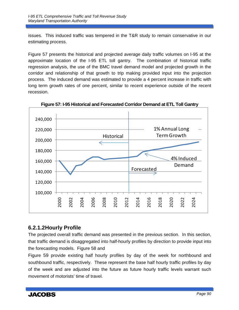
I-95 ETL Comprehensive Traffic and Toll Revenue Study Maryland Transportation Authority
Page 90
issues. This induced traffic was tempered in the T&R study to remain conservative in our estimating process. Figure 57 presents the historical and projected average daily traffic volumes on I-95 at the approximate location of the I-95 ETL toll gantry. The combination of historical traffic regression analysis, the use of the BMC travel demand model and projected growth in the corridor and relationship of that growth to trip making provided input into the projection process. The induced demand was estimated to provide a 4 percent increase in traffic with long term growth rates of one percent, similar to recent experience outside of the recent recession.
Figure 57: I-95 Historical and Forecasted Corridor Demand at ETL Toll Gantry
6.2.1.2 Hourly Profile The projected overall traffic demand was presented in the previous section. In this section,
that traffic demand is disaggregated into half-hourly profiles by direction to provide input into
the forecasting models. Figure 58 and
Figure 59 provide existing half hourly profiles by day of the week for northbound and
southbound traffic, respectively. These represent the base half hourly traffic profiles by day
of the week and are adjusted into the future as future hourly traffic levels warrant such
movement of motorists’ time of travel.
100,000
120,000
140,000
160,000
180,000
200,000
220,000
240,000
2000
2002
2004
2006
2008
2010
2012
2014
2016
2018
2020
2022
2024
Historical
Forecasted
4% Induced Demand
1%Annual Long Term Growth

I-95 ETL Comprehensive Traffic and Toll Revenue Study Maryland Transportation Authority
Page 91
Figure 58: Northbound Half-Hour Profiles by Day of the Week
Figure 59: Southbound Half-Hour Profiles by Day of the Week
0.0%
0.5%
1.0%
1.5%
2.0%
2.5%
3.0%
3.5%
4.0%
4.5%
5.0%
0:00
1:00
2:00
3:00
4:00
5:00
6:00
7:00
8:00
9:00
10:00
11:00
12:00
13:00
14:00
15:00
16:00
17:00
18:00
19:00
20:00
21:00
22:00
23:00
Sun
Mon
Tue
Wed
Thu
Fri
Sat
0.0%
0.5%
1.0%
1.5%
2.0%
2.5%
3.0%
3.5%
4.0%
4.5%
5.0%
0:00
1:00
2:00
3:00
4:00
5:00
6:00
7:00
8:00
9:00
10:00
11:00
12:00
13:00
14:00
15:00
16:00
17:00
18:00
19:00
20:00
21:00
22:00
23:00
Sun
Mon
Tue
Wed
Thu
Fri
Sat
I-95 ETL Comprehensive Traffic and Toll Revenue Study Maryland Transportation Authority
Page 92
6.2.1.3 Other T&R Assumptions In addition to the major assumptions affecting the T&R analysis of corridor demand and hourly profiles, there are a myriad of other assumptions, including vehicle class by hour, payment classes, violation rates and ramp-up that were presented previously in Figure 54. The assumption of the percentage of trucks in the corridor is varied by day of the week and hour of the day based on existing traffic volumes. These percentages range from 6 to 30 percent in the corridor. The values of time in the corridor were derived from stated preference survey conducted and documented within this report which uses a range of values of time from $7.79 to $16.90 depending on time period and payment method. These stated values of time were combined in the model with revealed values of time on managed lane facilities across the United States as people are making real decisions in the lanes. The percentage of transactions collected by E-ZPass was developed as a function of day of the week and hour of the day as seen on other facilities. The I-95 ETL will be fully electronic so transactions outside of E-ZPass will be collected via capture of license plate. It is anticipated these video rates will range from 5 to 10 percent as a function of time of day. Ramp-up is a phenomenon in toll road forecasting that relates to the amount of time it takes motorists to fully understand the location and operation of the new toll facility and use it. The modeling that is conducted assumes full knowledge of the toll facility and the value it provides. On fully Greenfield facilities, those toll facilities that are on new ground, ramp-up is up to five years with discounts to modeled traffic up to 50 percent. The I-95 ETL is in the existing I-95 corridor and motorists have seen the construction for a number of years. The opening of the toll lanes will require some adjustment period, but is estimated to be rather quick. For this analysis it is assumed the ramp-up period will be two years with discounts to traffic and toll revenue of 15 and 5 percent by year, respectively. The final assumption is related to violation rates. The forecasted transactions assume a level of loss due to either bad reads of an E-ZPass, two percent loss, or inability to collect a video toll, 30 percent loss. These losses are incorporated into the forecasts provided.
6.3 Toll Sensitivity Analyses Toll sensitivity analyses were conducted to provide insight into the relationship between ETL traffic, toll rate, and toll revenue. For the I-95 ETL, this relationship is rather complicated since it is also a function of corridor demand as the toll schedule will
I-95 ETL Comprehensive Traffic and Toll Revenue Study Maryland Transportation Authority
Page 93
necessarily change to manage traffic in the ETL. This being the case, toll sensitivity analyses were first conducted for various corridor demands to illustrate the potential toll revenue across any year or time period. Then toll sensitivity analyses were conducted for peak, off-peak and overnight time periods. In this section, first the toll sensitivity of passenger cars is presented and then the same is presented for commercial vehicles.
6.3.1 Passenger Cars Figure 60 presents the relationship between hourly traffic on the ETL and toll rate as a function of corridor demand. For instance, assuming a corridor demand of 8,500, it is estimated that there are approximately 2,500 vehicles in the ETL at a per mile toll rate of $0.10. This volume decreases as the toll rate increases. Similarly, the volume also decreases as the corridor demand decreases. For instance, at $0.20 per mile, assuming a corridor demand of 8,000 vehicles, it is estimated only 2,000 vehicles will choose the ETL as compared to 2,500 for 8,500 corridor demand and $0.20 per mile toll rate. As the corridor demand decreases, the estimated volumes of motorists choosing the ETL decrease. This is because time savings in the ETL is a function of congestion on the toll-free general purpose lanes which is a function of overall corridor demand.

I-95 ETL Comprehensive Traffic and Toll Revenue Study Maryland Transportation Authority
Page 94
Figure 60: ETL Hourly Traffic Volumes as a Function of Toll Rate and Corridor Demand
Figure 61 uses the same analysis that is presented in Figure 60 and provides estimated hourly toll revenue as a function of toll rate and hourly corridor demand. As traffic decreases with an increase in toll rate, there is a point when toll revenue will stop increasing as it is estimated that the loss in traffic cannot be made-up by the increase in the toll rate. These maximum points in the curves are defined as the toll revenue maximizing toll rates. As corridor demand increases, it is apparent that the toll revenue maximizing toll rates increase as well. For low corridor volumes of 7,000 and below the toll revenue maximizing toll rates are estimated to be between $0.20 and $0.40 cents per mile. At these low levels of corridor demand, the time savings is minimal and such that the toll rate can only increase a limited amount until it is estimated no motorists would choose the ETL. For higher levels of corridor demand, the toll revenue maximizing toll rates are estimated to be quite high, with corridor demand of 8,500, the revenue maximizing toll rate of $1.20 is estimated. At these levels of corridor demand, time savings is significant. Figure 62 presents the estimated potential hourly revenue as a function of corridor demand for the ETL. The salient point of this graph is the quick increase in potential toll revenue as corridor demand rises. There is very limited revenue potential until congestion hits the corridor, which is evident in this graph. It mirrors the speed deterioration curves presented in the data collection portion of this document. There is a steep relationship between
0
500
1000
1500
2000
2500
3000
$0.000 $0.200 $0.400 $0.600 $0.800 $1.000 $1.200 $1.400
ETL Hourly Traffic Volume
Per Mile Toll Rate
Relationship between ETL Volume and Toll Rate holding Hourly Corridor Demand constant
6000
6500
7000
7500
8000
8500
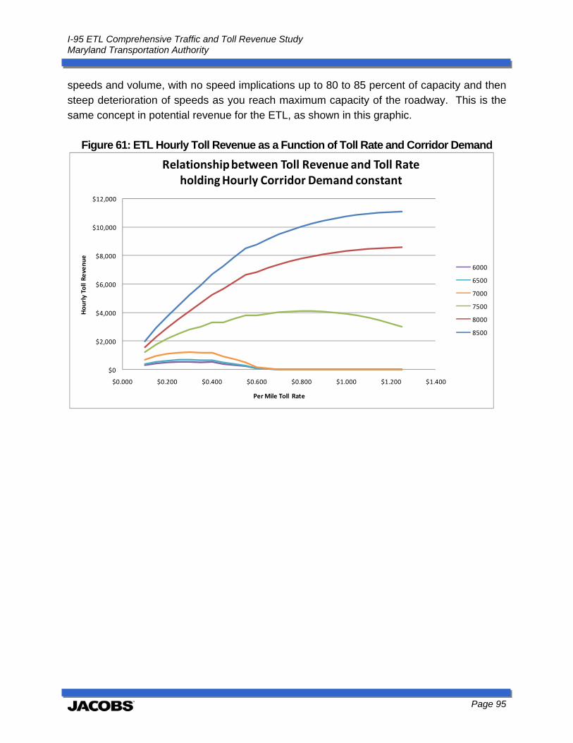
I-95 ETL Comprehensive Traffic and Toll Revenue Study Maryland Transportation Authority
Page 95
speeds and volume, with no speed implications up to 80 to 85 percent of capacity and then steep deterioration of speeds as you reach maximum capacity of the roadway. This is the same concept in potential revenue for the ETL, as shown in this graphic.
Figure 61: ETL Hourly Toll Revenue as a Function of Toll Rate and Corridor Demand
$0
$2,000
$4,000
$6,000
$8,000
$10,000
$12,000
$0.000 $0.200 $0.400 $0.600 $0.800 $1.000 $1.200 $1.400
Hourly Toll Revenue
Per Mile Toll Rate
Relationship between Toll Revenue and Toll Rate holding Hourly Corridor Demand constant
6000
6500
7000
7500
8000
8500
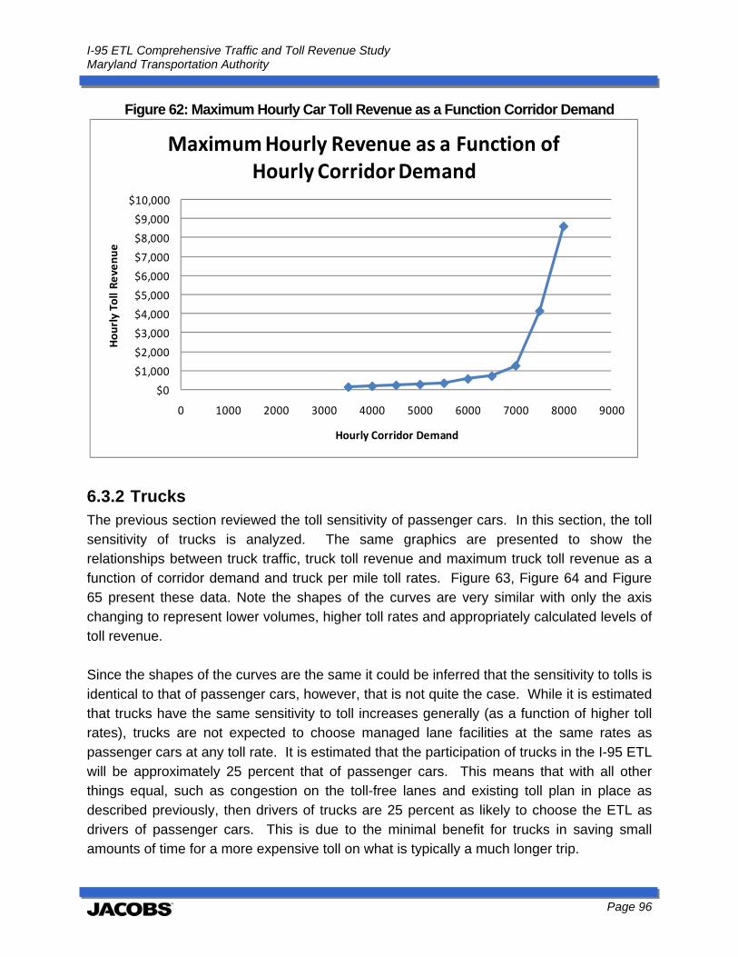
I-95 ETL Comprehensive Traffic and Toll Revenue Study Maryland Transportation Authority
Page 96
Figure 62: Maximum Hourly Car Toll Revenue as a Function Corridor Demand
6.3.2 Trucks The previous section reviewed the toll sensitivity of passenger cars. In this section, the toll sensitivity of trucks is analyzed. The same graphics are presented to show the relationships between truck traffic, truck toll revenue and maximum truck toll revenue as a function of corridor demand and truck per mile toll rates. Figure 63, Figure 64 and Figure 65 present these data. Note the shapes of the curves are very similar with only the axis changing to represent lower volumes, higher toll rates and appropriately calculated levels of toll revenue. Since the shapes of the curves are the same it could be inferred that the sensitivity to tolls is identical to that of passenger cars, however, that is not quite the case. While it is estimated that trucks have the same sensitivity to toll increases generally (as a function of higher toll rates), trucks are not expected to choose managed lane facilities at the same rates as passenger cars at any toll rate. It is estimated that the participation of trucks in the I-95 ETL will be approximately 25 percent that of passenger cars. This means that with all other things equal, such as congestion on the toll-free lanes and existing toll plan in place as described previously, then drivers of trucks are 25 percent as likely to choose the ETL as drivers of passenger cars. This is due to the minimal benefit for trucks in saving small amounts of time for a more expensive toll on what is typically a much longer trip.
$0
$1,000
$2,000
$3,000
$4,000
$5,000
$6,000
$7,000
$8,000
$9,000
$10,000
0 1000 2000 3000 4000 5000 6000 7000 8000 9000
Hourly Toll Revenue
Hourly Corridor Demand
Maximum Hourly Revenue as a Function of Hourly Corridor Demand
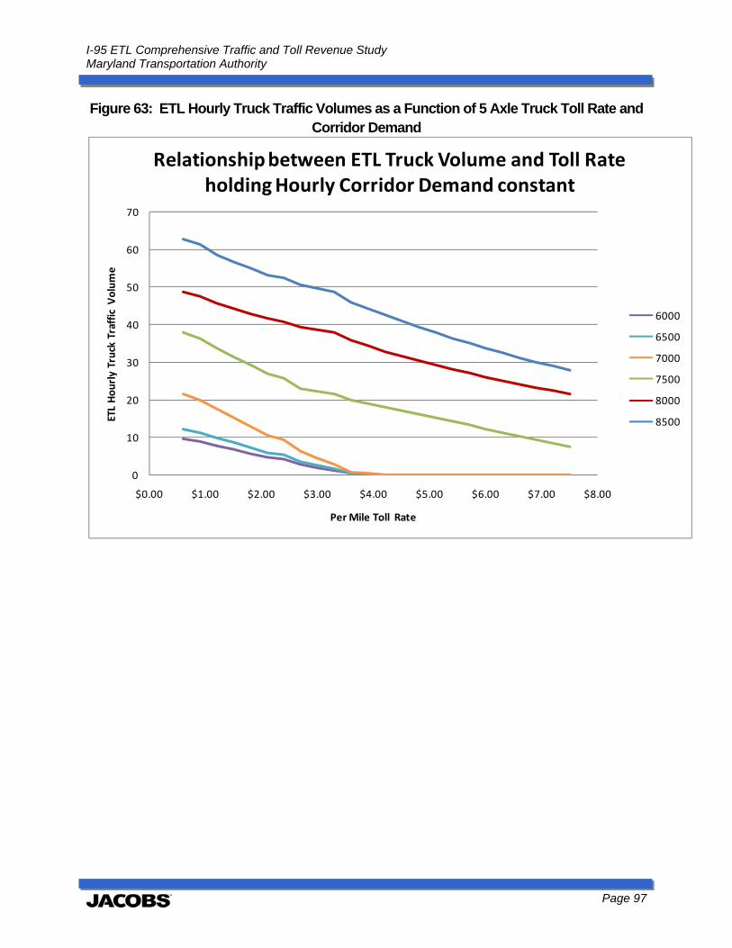
I-95 ETL Comprehensive Traffic and Toll Revenue Study Maryland Transportation Authority
Page 97
Figure 63: ETL Hourly Truck Traffic Volumes as a Function of 5 Axle Truck Toll Rate and Corridor Demand
0
10
20
30
40
50
60
70
$0.00 $1.00 $2.00 $3.00 $4.00 $5.00 $6.00 $7.00 $8.00
ETL Hourly Truck Traffic V
olume
Per Mile Toll Rate
Relationship between ETL Truck Volume and Toll Rate holding Hourly Corridor Demand constant
6000
6500
7000
7500
8000
8500
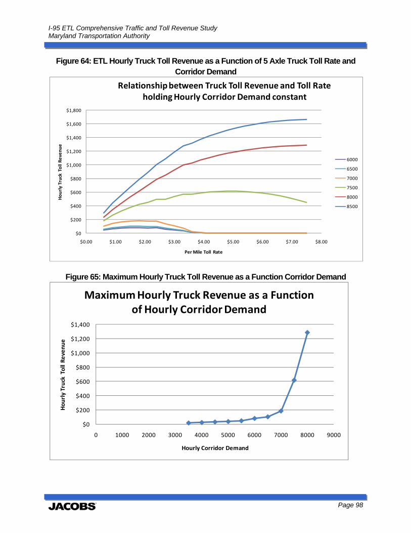
I-95 ETL Comprehensive Traffic and Toll Revenue Study Maryland Transportation Authority
Page 98
Figure 64: ETL Hourly Truck Toll Revenue as a Function of 5 Axle Truck Toll Rate and Corridor Demand
Figure 65: Maximum Hourly Truck Toll Revenue as a Function Corridor Demand
$0
$200
$400
$600
$800
$1,000
$1,200
$1,400
$1,600
$1,800
$0.00 $1.00 $2.00 $3.00 $4.00 $5.00 $6.00 $7.00 $8.00
Hourly Truck Toll Revenue
Per Mile Toll Rate
Relationship between Truck Toll Revenue and Toll Rate holding Hourly Corridor Demand constant
6000
6500
7000
7500
8000
8500
$0
$200
$400
$600
$800
$1,000
$1,200
$1,400
0 1000 2000 3000 4000 5000 6000 7000 8000 9000
Hourly Truck Toll Revenue
Hourly Corridor Demand
Maximum Hourly Truck Revenue as a Function of Hourly Corridor Demand
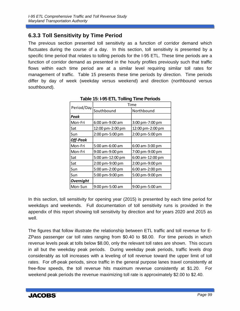
I-95 ETL Comprehensive Traffic and Toll Revenue Study Maryland Transportation Authority
Page 99
6.3.3 Toll Sensitivity by Time Period The previous section presented toll sensitivity as a function of corridor demand which fluctuates during the course of a day. In this section, toll sensitivity is presented by a specific time period that relates to tolling periods for the I-95 ETL. These time periods are a function of corridor demand as presented in the hourly profiles previously such that traffic flows within each time period are at a similar level requiring similar toll rates for management of traffic. Table 15 presents these time periods by direction. Time periods differ by day of week (weekday versus weekend) and direction (northbound versus southbound).
Table 15: I-95 ETL Tolling Time Periods
In this section, toll sensitivity for opening year (2015) is presented by each time period for weekdays and weekends. Full documentation of toll sensitivity runs is provided in the appendix of this report showing toll sensitivity by direction and for years 2020 and 2015 as well. The figures that follow illustrate the relationship between ETL traffic and toll revenue for E-ZPass passenger car toll rates ranging from $0.40 to $8.00. For time periods in which revenue levels peak at tolls below $8.00, only the relevant toll rates are shown. This occurs in all but the weekday peak periods. During weekday peak periods, traffic levels drop considerably as toll increases with a leveling of toll revenue toward the upper limit of toll rates. For off-peak periods, since traffic in the general purpose lanes travel consistently at free-flow speeds, the toll revenue hits maximum revenue consistently at $1.20. For weekend peak periods the revenue maximizing toll rate is approximately $2.00 to $2.40.
Southbound Northbound
Peak
Mon‐Fri 6:00 am‐9:00 am 3:00 pm‐7:00 pm
Sat 12:00 pm‐2:00 pm 12:00 pm‐2:00 pm
Sun 2:00 pm‐5:00 pm 2:00 pm‐5:00 pm
Off‐Peak
Mon‐Fri 5:00 am‐6:00 am 6:00 am‐3:00 pm
Mon‐Fri 9:00 am‐9:00 pm 7:00 pm‐9:00 pm
Sat 5:00 am‐12:00 pm 6:00 am‐12:00 pm
Sat 2:00 pm‐9:00 pm 2:00 pm‐9:00 pm
Sun 5:00 am‐2:00 pm 6:00 am‐2:00 pm
Sun 5:00 pm‐9:00 pm 5:00 pm‐9:00 pm
Overnight
Mon‐Sun 9:00 pm‐5:00 am 9:00 pm‐5:00 am
Period/DayTime

I-95 ETL Comprehensive Traffic and Toll Revenue Study Maryland Transportation Authority
Page 100
Figure 66: I-95 ETL Toll Sensitivity, Weekday Peak, 2015
Figure 67: I-95 ETL Toll Sensitivity, Weekday Off-Peak, 2015
0
5,000
10,000
15,000
20,000
25,000
30,000
35,000
40,000
0
500,000
1,000,000
1,500,000
2,000,000
2,500,000
3,000,000
3,500,000
4,000,000
4,500,000$0.40
$0.80
$1.20
$1.60
$2.00
$2.40
$2.80
$3.20
$3.60
$4.00
$4.40
$4.80
$5.20
$5.60
$6.00
$6.40
$6.80
$7.20
$7.60
$8.00
Weekly Traffic
Annual Toll Revenue
Passenger Car E‐ZPass Toll
Total Weekday Peak
Total Weekday Peak Revenue
Total Weekday Peak Traffic
0
5000
10000
15000
20000
25000
0.00
200,000.00
400,000.00
600,000.00
800,000.00
1,000,000.00
1,200,000.00
1,400,000.00
$0.40 $0.80 $1.20 $1.60 $2.00 $2.40 $2.80 $3.20 $3.60
Weekly Traffic
Annual Toll Revenue
Passenger Car E‐ZPass Toll
Total Weekday Off‐Peak
Total Weekday Off‐Peak Revenue
Total Weekday Off‐Peak Traffic
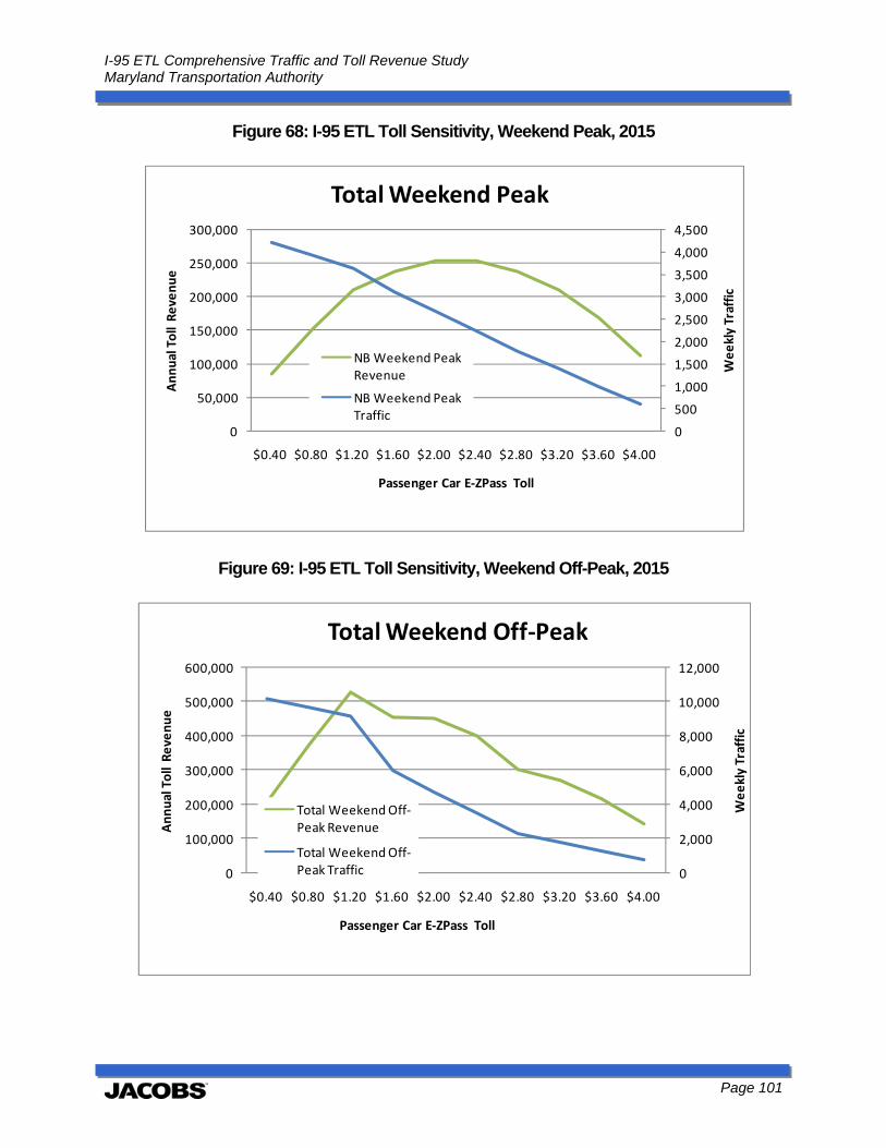
I-95 ETL Comprehensive Traffic and Toll Revenue Study Maryland Transportation Authority
Page 101
Figure 68: I-95 ETL Toll Sensitivity, Weekend Peak, 2015
Figure 69: I-95 ETL Toll Sensitivity, Weekend Off-Peak, 2015
0
500
1,000
1,500
2,000
2,500
3,000
3,500
4,000
4,500
0
50,000
100,000
150,000
200,000
250,000
300,000
$0.40 $0.80 $1.20 $1.60 $2.00 $2.40 $2.80 $3.20 $3.60 $4.00
Weekly Traffic
Annual Toll Revenue
Passenger Car E‐ZPass Toll
Total Weekend Peak
NB Weekend Peak Revenue
NB Weekend Peak Traffic
0
2,000
4,000
6,000
8,000
10,000
12,000
0
100,000
200,000
300,000
400,000
500,000
600,000
$0.40 $0.80 $1.20 $1.60 $2.00 $2.40 $2.80 $3.20 $3.60 $4.00
Weekly Traffic
Annual Toll Revenue
Passenger Car E‐ZPass Toll
Total Weekend Off‐Peak
Total Weekend Off‐Peak Revenue
Total Weekend Off‐Peak Traffic
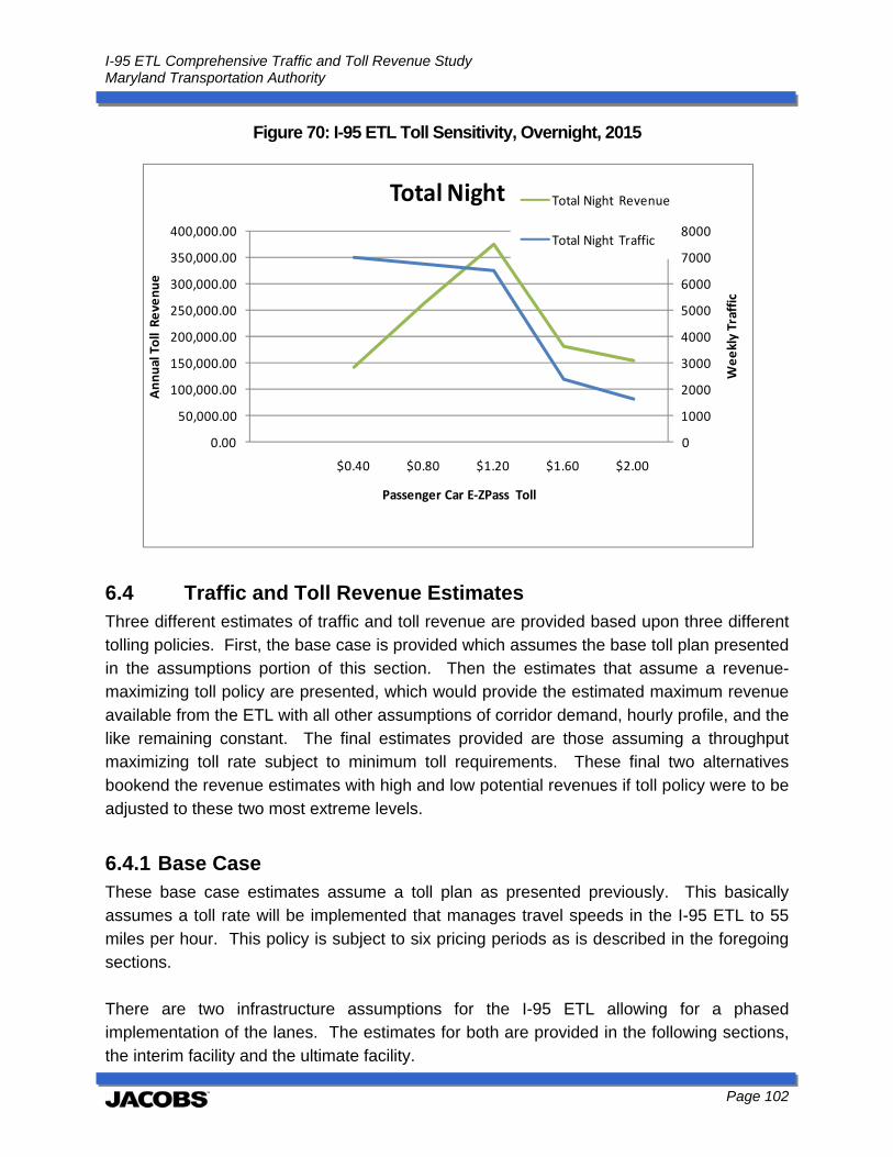
I-95 ETL Comprehensive Traffic and Toll Revenue Study Maryland Transportation Authority
Page 102
Figure 70: I-95 ETL Toll Sensitivity, Overnight, 2015
6.4 Traffic and Toll Revenue Estimates Three different estimates of traffic and toll revenue are provided based upon three different tolling policies. First, the base case is provided which assumes the base toll plan presented in the assumptions portion of this section. Then the estimates that assume a revenue-maximizing toll policy are presented, which would provide the estimated maximum revenue available from the ETL with all other assumptions of corridor demand, hourly profile, and the like remaining constant. The final estimates provided are those assuming a throughput maximizing toll rate subject to minimum toll requirements. These final two alternatives bookend the revenue estimates with high and low potential revenues if toll policy were to be adjusted to these two most extreme levels.
6.4.1 Base Case These base case estimates assume a toll plan as presented previously. This basically assumes a toll rate will be implemented that manages travel speeds in the I-95 ETL to 55 miles per hour. This policy is subject to six pricing periods as is described in the foregoing sections. There are two infrastructure assumptions for the I-95 ETL allowing for a phased implementation of the lanes. The estimates for both are provided in the following sections, the interim facility and the ultimate facility.
0
1000
2000
3000
4000
5000
6000
7000
8000
0.00
50,000.00
100,000.00
150,000.00
200,000.00
250,000.00
300,000.00
350,000.00
400,000.00
$0.40 $0.80 $1.20 $1.60 $2.00
Weekly Traffic
Annual Toll Revenue
Passenger Car E‐ZPass Toll
Total Night Total Night Revenue
Total Night Traffic
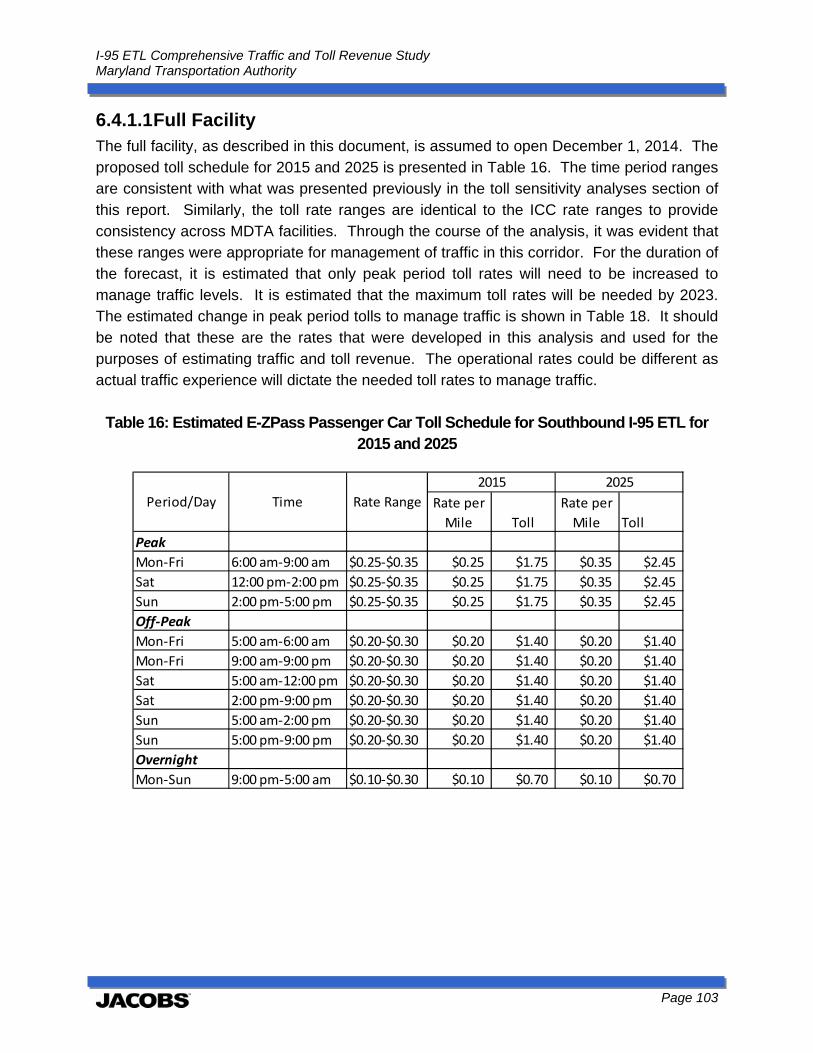
I-95 ETL Comprehensive Traffic and Toll Revenue Study Maryland Transportation Authority
Page 103
6.4.1.1 Full Facility The full facility, as described in this document, is assumed to open December 1, 2014. The proposed toll schedule for 2015 and 2025 is presented in Table 16. The time period ranges are consistent with what was presented previously in the toll sensitivity analyses section of this report. Similarly, the toll rate ranges are identical to the ICC rate ranges to provide consistency across MDTA facilities. Through the course of the analysis, it was evident that these ranges were appropriate for management of traffic in this corridor. For the duration of the forecast, it is estimated that only peak period toll rates will need to be increased to manage traffic levels. It is estimated that the maximum toll rates will be needed by 2023. The estimated change in peak period tolls to manage traffic is shown in Table 18. It should be noted that these are the rates that were developed in this analysis and used for the purposes of estimating traffic and toll revenue. The operational rates could be different as actual traffic experience will dictate the needed toll rates to manage traffic.
Table 16: Estimated E-ZPass Passenger Car Toll Schedule for Southbound I-95 ETL for 2015 and 2025
Rate per
Mile Toll
Rate per
Mile Toll
Peak
Mon‐Fri 6:00 am‐9:00 am $0.25‐$0.35 $0.25 $1.75 $0.35 $2.45
Sat 12:00 pm‐2:00 pm $0.25‐$0.35 $0.25 $1.75 $0.35 $2.45
Sun 2:00 pm‐5:00 pm $0.25‐$0.35 $0.25 $1.75 $0.35 $2.45
Off‐Peak
Mon‐Fri 5:00 am‐6:00 am $0.20‐$0.30 $0.20 $1.40 $0.20 $1.40
Mon‐Fri 9:00 am‐9:00 pm $0.20‐$0.30 $0.20 $1.40 $0.20 $1.40
Sat 5:00 am‐12:00 pm $0.20‐$0.30 $0.20 $1.40 $0.20 $1.40
Sat 2:00 pm‐9:00 pm $0.20‐$0.30 $0.20 $1.40 $0.20 $1.40
Sun 5:00 am‐2:00 pm $0.20‐$0.30 $0.20 $1.40 $0.20 $1.40
Sun 5:00 pm‐9:00 pm $0.20‐$0.30 $0.20 $1.40 $0.20 $1.40
Overnight
Mon‐Sun 9:00 pm‐5:00 am $0.10‐$0.30 $0.10 $0.70 $0.10 $0.70
Period/Day Time Rate Range
2015 2025

I-95 ETL Comprehensive Traffic and Toll Revenue Study Maryland Transportation Authority
Page 104
Table 17: Estimated E-ZPass Passenger Car Toll Schedule for Northbound I-95 ETL for 2015 and 2025
Table 18: Estimated Peak Period E-ZPass Passenger Car Tolls for I-95 ETL, 2015 to 2025
With this toll schedule in place and the assumptions presented in this document, the estimates of annual traffic and toll revenue are presented in Table 19. It is estimated that traffic on the ETL will grow at an average annual rate of 5.7 percent and toll revenue will grow at 8.3 percent. The cause for this discrepancy is the estimated needed increase in tolls to manage traffic during peak travel periods as shown in Table 16. This same information is illustrated in Figure 71 to more clearly identify the differences in growth rates.
Rate per
Mile Toll
Rate per
Mile Toll
Peak
Mon‐Fri 6:00 am‐9:00 am $0.25‐$0.35 $0.25 $1.75 $0.35 $2.45
Sat 12:00 pm‐2:00 pm $0.25‐$0.35 $0.25 $1.75 $0.35 $2.45
Sun 2:00 pm‐5:00 pm $0.25‐$0.35 $0.25 $1.75 $0.35 $2.45
Off‐Peak
Mon‐Fri 5:00 am‐6:00 am $0.20‐$0.30 $0.20 $1.40 $0.20 $1.40
Mon‐Fri 9:00 am‐9:00 pm $0.20‐$0.30 $0.20 $1.40 $0.20 $1.40
Sat 5:00 am‐12:00 pm $0.20‐$0.30 $0.20 $1.40 $0.20 $1.40
Sat 2:00 pm‐9:00 pm $0.20‐$0.30 $0.20 $1.40 $0.20 $1.40
Sun 5:00 am‐2:00 pm $0.20‐$0.30 $0.20 $1.40 $0.20 $1.40
Sun 5:00 pm‐9:00 pm $0.20‐$0.30 $0.20 $1.40 $0.20 $1.40
Overnight
Mon‐Sun 9:00 pm‐5:00 am $0.10‐$0.30 $0.10 $0.70 $0.10 $0.70
Period/Day Time Rate Range
2015 2025
Year Peak Period Toll
2015 $1.75
2016 $1.75
2017 $1.75
2018 $1.75
2019 $1.75
2020 $1.90
2021 $2.05
2022 $2.15
2023 $2.45
2024 $2.45
2025 $2.45
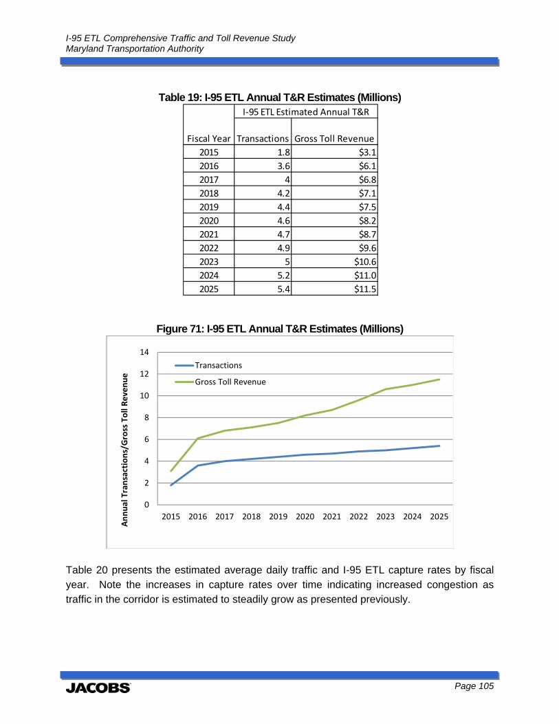
I-95 ETL Comprehensive Traffic and Toll Revenue Study Maryland Transportation Authority
Page 105
Table 19: I-95 ETL Annual T&R Estimates (Millions)
Figure 71: I-95 ETL Annual T&R Estimates (Millions)
Table 20 presents the estimated average daily traffic and I-95 ETL capture rates by fiscal year. Note the increases in capture rates over time indicating increased congestion as traffic in the corridor is estimated to steadily grow as presented previously.
Transactions Gross Toll Revenue
2015 1.8 $3.1
2016 3.6 $6.1
2017 4 $6.8
2018 4.2 $7.1
2019 4.4 $7.5
2020 4.6 $8.2
2021 4.7 $8.7
2022 4.9 $9.6
2023 5 $10.6
2024 5.2 $11.0
2025 5.4 $11.5
Fiscal Year
I‐95 ETL Estimated Annual T&R
0
2
4
6
8
10
12
14
2015 2016 2017 2018 2019 2020 2021 2022 2023 2024 2025
Annual Transactions/Gross Toll Revenue
Transactions
Gross Toll Revenue

I-95 ETL Comprehensive Traffic and Toll Revenue Study Maryland Transportation Authority
Page 106
Table 20: Estimated I-95 Average Daily Traffic and ETL Capture Rates
As stated previously, the estimates presented in this section do not take into account the benefit of alternative toll schedules during holiday events that will likely provide slight marginal benefit to presented traffic and toll revenue. This slight benefit was deemed not significant enough to incorporate into these estimates of annual revenue.
6.4.2 Revenue Maximizing In addition to the base case which employs the tolling policy identified in the assumptions of the analysis, a sensitivity test was run assuming toll revenue maximizing toll rates were implemented. This revenue sensitivity analysis used the results of the toll sensitivity analyses which determined the toll revenue maximizing toll rates by time period. Those toll revenue maximizing rates were then applied in the forecasting model and the appropriate levels of estimated traffic and toll revenue from the I-95 ETL were estimated. All other assumptions of value of time, corridor growth, violations and the like were held constant from the base case to this sensitivity test to reflect only the change in toll policy. Table 21 presents the estimates of traffic and toll revenue for this revenue maximizing case. The traffic is considerably lower as compared to the base case with revenue much higher. By year the traffic is between 14 and 27 percent lower than the base case with toll revenue between 36 and 62 percent higher.
Toll‐Free General
Purpose
Express
Toll LanesTotal Capture Rate
2015 167,322 10,038 177,360 5.7%
2016 168,666 10,468 179,134 5.8%
2017 169,916 11,009 180,925 6.1%
2018 171,163 11,571 182,734 6.3%
2019 172,468 12,093 184,562 6.6%
2020 173,824 12,583 186,407 6.8%
2021 175,519 12,752 188,271 6.8%
2022 176,672 13,482 190,154 7.1%
2023 178,395 13,660 192,055 7.1%
2024 179,824 14,152 193,976 7.3%
2025 181,074 14,842 195,916 7.6%
Fiscal Year
Estimated I‐95 Traffic
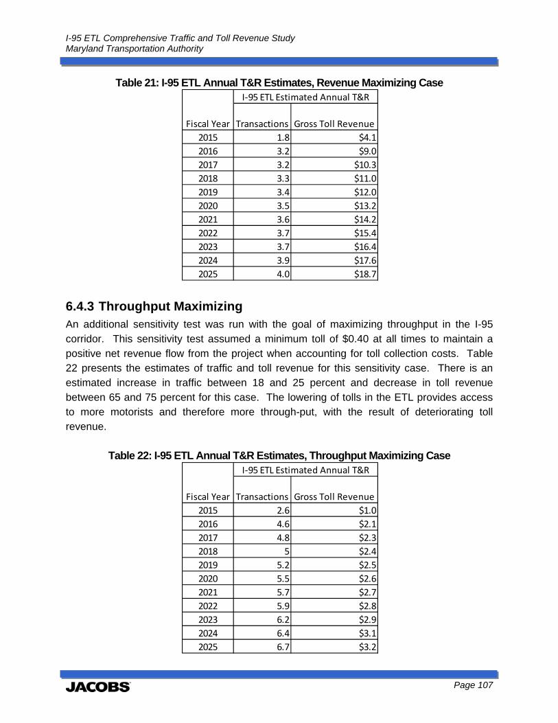
I-95 ETL Comprehensive Traffic and Toll Revenue Study Maryland Transportation Authority
Page 107
Table 21: I-95 ETL Annual T&R Estimates, Revenue Maximizing Case
6.4.3 Throughput Maximizing An additional sensitivity test was run with the goal of maximizing throughput in the I-95 corridor. This sensitivity test assumed a minimum toll of $0.40 at all times to maintain a positive net revenue flow from the project when accounting for toll collection costs. Table 22 presents the estimates of traffic and toll revenue for this sensitivity case. There is an estimated increase in traffic between 18 and 25 percent and decrease in toll revenue between 65 and 75 percent for this case. The lowering of tolls in the ETL provides access to more motorists and therefore more through-put, with the result of deteriorating toll revenue.
Table 22: I-95 ETL Annual T&R Estimates, Throughput Maximizing Case
Transactions Gross Toll Revenue
2015 1.8 $4.1
2016 3.2 $9.0
2017 3.2 $10.3
2018 3.3 $11.0
2019 3.4 $12.0
2020 3.5 $13.2
2021 3.6 $14.2
2022 3.7 $15.4
2023 3.7 $16.4
2024 3.9 $17.6
2025 4.0 $18.7
Fiscal Year
I‐95 ETL Estimated Annual T&R
Transactions Gross Toll Revenue
2015 2.6 $1.0
2016 4.6 $2.1
2017 4.8 $2.3
2018 5 $2.4
2019 5.2 $2.5
2020 5.5 $2.6
2021 5.7 $2.7
2022 5.9 $2.8
2023 6.2 $2.9
2024 6.4 $3.1
2025 6.7 $3.2
Fiscal Year
I‐95 ETL Estimated Annual T&R

I-95 ETL Comprehensive Traffic and Toll Revenue Study Maryland Transportation Authority
Page 108
The base case and sensitivity tests have an impact on travel speeds in the corridor. The base case is held to maintaining a speed of 55 miles per hour in the ETL subject to ICC toll rate ranges, while the two sensitivity cases disregard this constraint and are held to either maximizing revenue or throughput (with the exception of a minimum toll held for this case). The impact on minimum travel speeds is presented in Table 23. In the base case, the minimum travel speeds for the ETL is held near 55 miles per hour per toll policy with the toll-free general purpose lanes being 42 miles per hour in 2015 retreating to 38 miles per hour in the latter years of the forecast. The same trend is seen for the revenue maximizing case except with the ETL having the maximum speed allowed of 65 miles per hour due to the limited number of vehicles in the lanes because of the higher toll rates. In this case, the speeds in the adjacent toll-free general purpose lanes are estimated to decrease from 27 miles per hour to 20 miles per hour during the forecast period. For the final sensitivity test, the throughput maximizing case, the travel speeds in the ETL and the general purpose lanes are much closer with travel speeds on the ETL of between 47 and 44 miles per hour and on the general purpose lanes of between 45 and 40 miles per hour as a function of year. These speed differentials depict the consequence of toll policy adjustment to the traffic operations in both the ETL and the general purpose lanes for this portion of the I-95 corridor.
Table 23: Estimated I-95 Corridor Minimum Speeds By Case
6.5 Risk Analysis In the preceding section the base case and sensitivity cases were presented to provide an understanding of the range of potential traffic and toll revenues with varying toll policies. In this section, a risk analysis of the potential traffic and toll revenue is presented to provide a
Express Toll
Lane
General
Purpose
Lane
Express Toll
Lane
General
Purpose
Lane
Express Toll
Lane
General
Purpose
Lane
2015 58 42 65 27 47 45
2016 58 42 65 26 47 45
2017 57 42 65 25 46 45
2018 56 41 65 25 46 44
2019 55 43 65 24 46 42
2020 55 42 65 24 45 42
2021 55 42 65 23 45 41
2022 55 42 65 23 45 41
2023 54 39 65 21 44 40
2024 54 39 65 20 44 40
2025 53 38 65 20 44 40
Year
Minimum Estimated Speed in the Corridor (mph)
Base Case Revenue Maximizing Throughput Maximizing
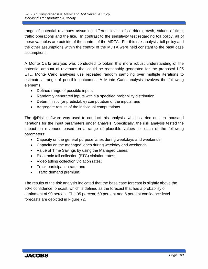
I-95 ETL Comprehensive Traffic and Toll Revenue Study Maryland Transportation Authority
Page 109
range of potential revenues assuming different levels of corridor growth, values of time, traffic operations and the like. In contrast to the sensitivity test regarding toll policy, all of these variables are outside of the control of the MDTA. For this risk analysis, toll policy and the other assumptions within the control of the MDTA were held constant to the base case assumptions. A Monte Carlo analysis was conducted to obtain this more robust understanding of the potential amount of revenues that could be reasonably generated for the proposed I-95 ETL. Monte Carlo analyses use repeated random sampling over multiple iterations to estimate a range of possible outcomes. A Monte Carlo analysis involves the following elements:
Defined range of possible inputs; Randomly generated inputs within a specified probability distribution; Deterministic (or predictable) computation of the inputs; and Aggregate results of the individual computations.
The @Risk software was used to conduct this analysis, which carried out ten thousand iterations for the input parameters under analysis. Specifically, the risk analysis tested the impact on revenues based on a range of plausible values for each of the following parameters:
Capacity on the general purpose lanes during weekdays and weekends; Capacity on the managed lanes during weekday and weekends; Value of Time Savings by using the Managed Lanes; Electronic toll collection (ETC) violation rates; Video tolling collection violation rates; Truck participation rate; and Traffic demand premium.
The results of the risk analysis indicated that the base case forecast is slightly above the 90% confidence forecast, which is defined as the forecast that has a probability of attainment of 90 percent. The 95 percent, 50 percent and 5 percent confidence level forecasts are depicted in Figure 72.
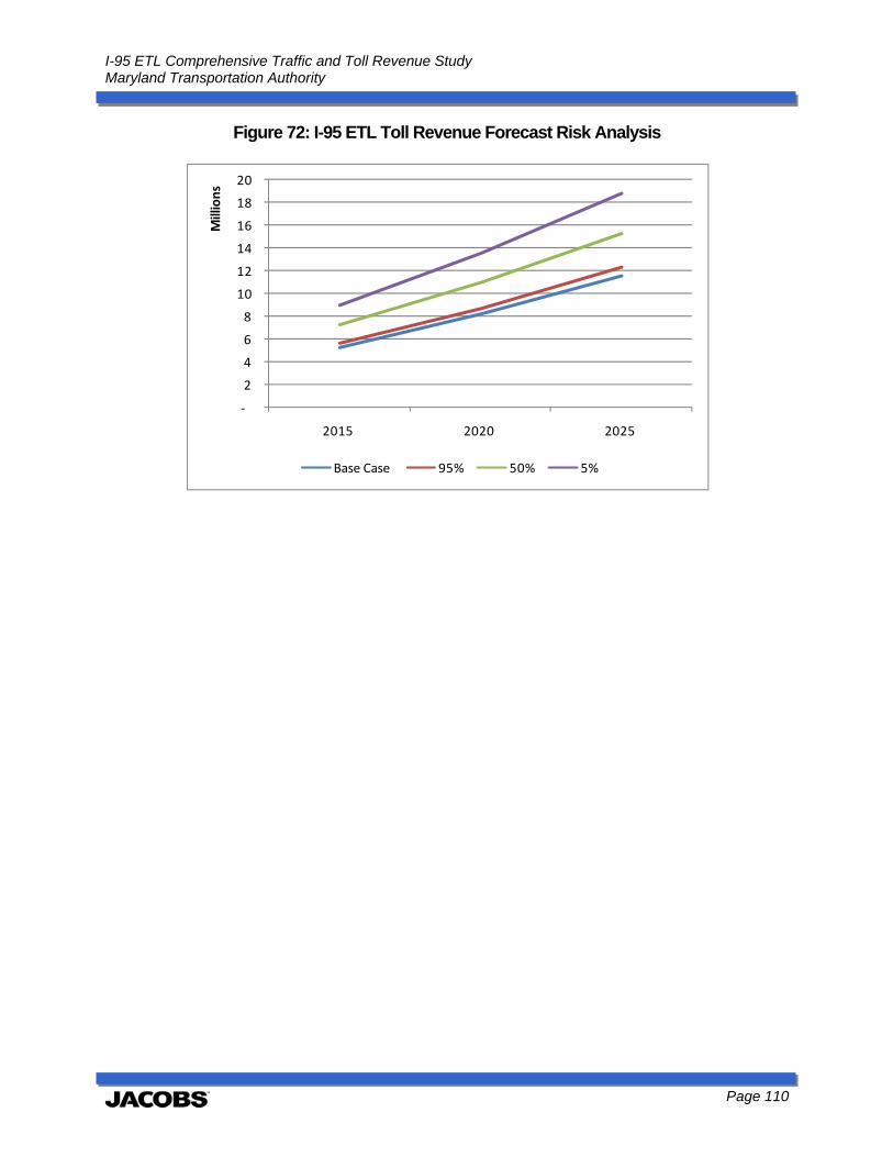
I-95 ETL Comprehensive Traffic and Toll Revenue Study Maryland Transportation Authority
Page 110
Figure 72: I-95 ETL Toll Revenue Forecast Risk Analysis
‐
2
4
6
8
10
12
14
16
18
20
2015 2020 2025
Millions
Base Case 95% 50% 5%
I-95 ETL Comprehensive Traffic and Toll Revenue Study Maryland Transportation Authority
Page 111
7.0 Limits and Disclaimers It is Jacobs’ opinion that the traffic and toll revenue estimates provided herein are reasonable and that they have been prepared in accordance with accepted industry-wide practice. However, given the uncertainties within the current economic climate, it is important to note the following assumptions which, in our opinion, are reasonable: This report presents the results of Jacobs’ consideration of the information available as
of the date hereof and the application of our experience and professional judgment to that information. It is not a guarantee of any future events or trends.
The traffic and toll revenue estimates will be subject to future economic and social conditions, demographic developments and regional transportation construction activities that cannot be predicted with certainty.
The estimates contained in this report, while presented with numeric specificity, are based on a number of estimates and assumptions which, though considered reasonable to us, are inherently subject to economic and competitive uncertainties and contingencies, most of which are beyond the control of the MDTA and cannot be predicted with certainty. In many instances, a broad range of alternative assumptions could be considered reasonable. Changes in the assumptions used could result in material differences in estimated outcomes.
Jacobs’ traffic and toll revenue estimations only represent our best judgment and we do not warrant or represent that the actual toll revenues will not vary from our estimates.
We do not express any opinion on the following items: socioeconomic and demographic forecasts, proposed land use development projects and potential improvements to the regional transportation network.
The standards of operation and maintenance on all of the system will be maintained as planned within the business rules and practices.
The general configuration and location of the system and its interchanges will remain as discussed in this report.
Access to and from the system will remain as discussed in this report.
No other competing highway projects, tolled or non-tolled, are assumed to be constructed or significantly improved in the project corridor during the project period, except those identified within this report.
Major highway improvements that are currently underway or fully funded will be completed as planned.
The system will be well maintained, efficiently operated, and effectively signed to encourage maximum usage.

I-95 ETL Comprehensive Traffic and Toll Revenue Study Maryland Transportation Authority
Page 112
No reduced growth initiatives or related controls that would significantly inhibit normal development patterns will be introduced during the estimate period.
There will be no future serious protracted recession during the estimate period.
There will be no protracted fuel shortage during the estimate period.
No local, regional, or national emergency will arise that will abnormally restrict the use of motor vehicles.
In Jacobs' opinion, the assumptions underlying the projections provide a reasonable basis for the revenue projections and operating expenses. However, any financial projection is subject to uncertainties. Inevitably, some assumptions used to develop the projections will not be realized, and unanticipated events and circumstances may occur. There are likely to be differences between the projections and actual results, and those differences may be material. Because of these uncertainties, Jacobs makes no guaranty or warranty with respect to the projections disclosed in this Study. * * * * * We greatly appreciate the invaluable assistance provided by the staff of the Maryland Transportation Authority. Very truly yours, Richard J. Gobeille, P.E. Phil Eshelman National Toll/Finance Unit Manager Project Manager

APPENDIX A
Stated Preference Survey Technical Memorandum
Jacobs Engineering
Value of Time of Motorists on I-95 ETLs
Final Technical Memorandum
February 5, 2013
451 Hungerford Drive, Suite 515 Rockville, MD 20850 www.eurekafacts.com 240.403.4800 866.693.2287 Contact:
Jorge Restrepo, CEO [email protected] Joanne Arnold, Director of Research Programs [email protected] Djass Mbangdadji, Chief Statistician [email protected]
Table of Contents
EXECUTIVE SUMMARY ................................................................................................. 1
INTRODUCTION ............................................................................................................. 3
METHODOLOGY ............................................................................................................ 4 Developing the Survey Instrument .......................................................................................... 4
Sampling ................................................................................................................................ 4
Data Collection ....................................................................................................................... 5
Statistical Analysis Techniques............................................................................................... 6
Willingness to Pay Analyses ................................................................................................... 6
RESULTS OF STATISTICAL ANALYSES ...................................................................... 8 Results for Non-E-ZPass Users .............................................................................................. 8
Results for E-ZPass Users ..................................................................................................... 9
E-ZPass Users Crosstab Results ........................................................................................ 9
E-ZPass Users Willingness to Pay Results ........................................................................18
Value of Time (VOT) Modeling Results ..............................................................................24
Calculation of the Value of Time (VOT) ..............................................................................24
QUESTIONNAIRE......................................................................................................... 34
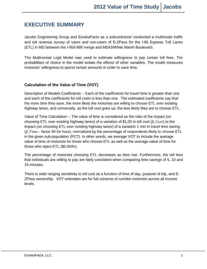
2012 Value of Time Study Jacobs
EurekaFacts, LLC 1
EXECUTIVE SUMMARY Jacobs Engineering Group and EurekaFacts as a subcontractor conducted a multimode traffic and toll revenue survey of users and non-users of E-ZPass for the I-95 Express Toll Lanes (ETL) in MD between the I-95/I-895 merge and MD43/White Marsh Boulevard. The Multinomial Logit Model was used to estimate willingness to pay certain toll fees. The probabilities of choice in the model isolate the effects of other variables. The model measures motorists’ willingness to spend certain amounts in order to save time.
Calculation of the Value of Time (VOT)
Description of Models Coefficients -- Each of the coefficients for travel time is greater than one and each of the coefficients for toll costs is less than one. The estimated coefficients say that the more time they save, the more likely the motorists are willing to choose ETL over existing highway lanes, and conversely, as the toll cost goes up, the less likely they are to choose ETL.
Value of Time Calculation -- The value of time is considered as the ratio of the impact (on choosing ETL over existing highway lanes) of a variation of $1.00 in toll cost (𝛽_𝐶𝑜𝑠𝑡) to the impact (on choosing ETL over existing highway lanes) of a variation 1 min in travel time saving (𝛽_𝑇𝑖𝑚𝑒 - factor 60 for hour), normalized by the percentage of respondents likely to choose ETL in the given sub-population (PCT). In other words, we average VOT to include the average value of time of motorists for those who choose ETL as well as the average value of time for those who reject ETL ($0.00/hr).
The percentage of motorists choosing ETL decreases as fees rise. Furthermore, the toll fees that individuals are willing to pay are fairly consistent when comparing time savings of 5, 10 and 15 minutes. There is wide ranging sensitivity to toll cost as a function of time of day, purpose of trip, and E-ZPass ownership. VOT estimates are for full universe of corridor motorists across all income levels.
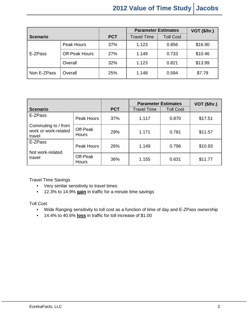
2012 Value of Time Study Jacobs
EurekaFacts, LLC 2
Travel Time Savings
• Very similar sensitivity to travel times • 12.3% to 14.9% gain in traffic for a minute time savings
Toll Cost
• Wide Ranging sensitivity to toll cost as a function of time of day and E-ZPass ownership • 14.4% to 40.6% loss in traffic for toll increase of $1.00
Scenario PCT
Parameter Estimates VOT ($/hr.) Travel Time Toll Cost
E-ZPass
Peak Hours 37% 1.123 0.856 $16.90
Off-Peak Hours 27% 1.149 0.733 $10.46
Overall 32% 1.123 0.821 $13.99
Non E-ZPass Overall 25% 1.148 0.594 $7.79
Scenario PCT Parameter Estimates VOT ($/hr.)
Travel Time Toll Cost E-ZPass Commuting to / from work or work-related travel
Peak Hours 37% 1.117 0.870 $17.51
Off-Peak Hours
29% 1.171 0.781 $11.57
E-ZPass Not work-related travel
Peak Hours 26% 1.149 0.796 $10.93
Off-Peak Hours
36% 1.155 0.631 $11.77
2012 Value of Time Study Jacobs
EurekaFacts, LLC 3
INTRODUCTION Jacobs Engineering Group Inc., one of the world’s largest and most diverse providers of professional technical services, was awarded the Maryland Transportation Authority (MDTA) T&R contract in 2009 with EurekaFacts serving as a subcontractor. Jacobs was directed to conduct a traffic and toll revenue study for the I-95 Express Toll Lanes (ETLs). EurekaFacts was tasked with gauging the perceptions of motorists’ value of time perceptions regarding ELTs under various conditions. The methods used included a mixed mode data collection approach including email, notification postcards, an online survey, and computer-assisted telephone interviewing (CATI) data collection. EurekaFacts developed the survey instrument with assistance from Jacobs Engineering. An online quantitative survey was conducted among E-ZPass user and non E-ZPass user vehicle owners residing in the area of I-95 of interest (the area between the I-95/I-895 merge and MD43/White Marsh Boulevard). In addition to vehicle and respondent demographic data, the survey yielded measurements of the incidence drivers are likely to consider ETL under various circumstances (scenarios) and the relationship between perceived time savings and the cost they would be willing to pay. Lastly, a nonlinear regression analysis was conducted to measure the probability of individuals choosing ETLs over other options. A linear model was not selected in order to account for the natural discrete choices presented to individuals. The data resulting from this study will be used as input into the Jacobs revenue forecasting model. Note: Results presented in this report are based on stated intentions and are not based
on actual behaviors.

2012 Value of Time Study Jacobs
EurekaFacts, LLC 4
METHODOLOGY Based upon a literature review and an investigation of previous related surveys, EurekaFacts developed an online survey instrument to record driver data including quantitatively measuring the value of time of motorists who use the section of I-95 of interest. The questionnaire was reviewed by Jacobs and approved after incorporating desired changes. To permit segmentation respondents were asked such questions about their most recent trip as trip origin, destination, purpose, day of week, time of the day, total travel time, travel frequency, as well as socio-economic demographic questions. The survey also contained preference scenario (trade-off) questions requiring respondents to choose between ELTs and other lanes under various conditions (peak/nonpeak, travel time savings, etc.) and the relationship between perceived time savings and the cost they would be willing to pay. The survey was administered to a sample of both E-ZPass users and non E-ZPass users. Using the data collected from the survey, EurekaFacts performed descriptive statistics, crosstabs, willingness to pay modeling, and regression analyses.
Developing the Survey Instrument The survey instrument was developed by EurekaFacts with assistance from Jacobs Engineering and MDTA. The instrument contained roughly 35 questions with a respondent burden of approximately 15 minutes to complete, depending on which scenario was presented to the respondent. The survey instrument included screener questions to ensure respondents are vehicle drivers familiar with the study area. The survey was pretested to 100 E-ZPass users. The instrument was inspected by a survey methods expert and then tested prior to deployment.
Sampling
To identify survey participants and obtain a balanced distribution of E-ZPass and non E-ZPass users along the I-95 Corridor, MDTA provided a list of 115,331 private vehicle E-ZPass users and 1,631 commercial vehicles whose owners reside in the geographic area covered by the study. The list contained email and mailing addresses. From this list a stratified sample was drawn containing 6,081 randomly selected private vehicle E-ZPass users and 1,169 commercial vehicle E-ZPass users. To identify candidate non-E-ZPass users, EurekaFacts purchased a list of vehicle owners residing in zip codes of the study as defined by Jacobs/MDTA and removing addresses of known E-ZPass users. This produced a list of 10,727 non E-ZPass users. Postcards containing a web link to an online survey were sent to the addresses in the sample, and email messages containing the invitation link were sent to those for whom an email address was known. A unique code was provided to each respondent in order to avoid multiple entries and manage sampling. Recipients of the email or postcard were encouraged to complete the online survey which was available 24/7. EurekaFacts programmed the survey instrument and
2012 Value of Time Study Jacobs
EurekaFacts, LLC 5
contacted non-respondents by telephone. The average time to administer the survey by CATI was also 15 minutes. EurekaFacts mailed postcards containing a link to an online survey to the vehicle owners without an E-ZPass account. Both E-ZPass users and non E-ZPass users who did not complete the survey online were then contacted and surveyed by telephone. EurekaFacts assigned each survey participant a unique ID to ensure only one response per person. The survey was fielded between November 1 and November 16, 2012. There were no disruptive incidents or notable events during the data collection period that could suggest biases or other limitations to the data collection effort.
Data Collection From this combined sample of 17,977 addresses, EurekaFacts obtained responses from 3,390 respondents. The survey yielded an overall response rate of 19% which is within the expected target. Response rates by group were: 22% among commercial vehicles, 42% among E-ZPass users and 5% among non E-ZPass users (the low response rate of the latter was not unexpected). The number of complete responses collected yielded a margin of error of + 4.0% for non-users, which is common in survey data. Percentages based on all 3,390 responses are subject to a ±1.5% margin of error at the 95% confidence level. In other words, for each sample size, one is 95% confident that the “true” percentage is in the region indicated by the corresponding segment with a ±1.5% margin of error. Table 1: Response Rate Breakdown
Respondent Vehicle Type Sample Raw Responses Raw Response Rate
E-ZPass users Commercial 1,169 259 22%
Private 6,081 2,560 42% Non E-ZPass users 10,727 571 5%
TOTAL 17,977 3,390 19%
2012 Value of Time Study Jacobs
EurekaFacts, LLC 6
For the purposes of analysis, we considered only complete and valid responses so individuals who did not answer at least one ETL question were removed from the sample. As a result, the number in the sample was reduced by about 1,000 cases. The reason for exclusion of cases was based on the screening due to non-use of the section of I-95 under study. The following table shows the total number of complete usable cases by survey mode. Table 2: Number Responding by Survey Mode Data Collection Mode No. Responding Percent
Email/Online 2,006 84% Postcard/Online 148 6% Telephone 242 10% Total 2,396 100%
Statistical Analysis Techniques
After examining response/non-response, EurekaFacts chose not to weight the data and instead conducted separate analyses of users and non-users. The differences introduced by survey mode included income and gender differences but were considered small enough not to warrant weighting. The large difference in sample sizes would have introduced large estimation errors in the more precise data set of E-ZPass users (who happen to be the main population of interest). EurekaFacts conducted descriptive analyses and cross-tabulations to obtain a picture of survey responses and respondents’ demographics. Various statistical analyses were conducted to provide additional insight into the parameters collected, including descriptive analysis, frequencies, crosstabs and chi-square tests. As a result, some variables’ categories were grouped to provide a more robust incidence of the variables associated with willingness to use ETL.
Willingness to Pay Analyses Willingness to pay is a choice modeling technique used to determine the maximum amount a person would be willing to pay or sacrifice to receive a good - in this case - a toll fee in exchange for faster ETL lanes. EurekaFacts estimated consumer willingness to pay using a multi-step modeling analysis to ascertain the likelihood to use ETL lanes. The analysis queried people to ascertain how they balance the cost of ETL lanes versus other factors, such as perceived time savings. Using this data, EurekaFacts generated an alternative pricing schedule for ETLs. In order to reduce fatigue and optimize data collection, respondents were asked only two or three different willingness to pay questions regarding time savings and toll fee levels. EurekaFacts used this data to extrapolate willingness to pay. Value of time is very heterogeneous among motorists (e.g., males have a different willingness to pay for ETL than females) and often depends on such socio-demographic factors as age,
2012 Value of Time Study Jacobs
EurekaFacts, LLC 7
gender and income. Even though pricing will not be based on demographics, understanding motorists’ differential willingness to pay for ETL is important in designing a price structure and finding the optimum price that could generate maximum revenue. For that reason, EurekaFacts analyzed responses to identify segments of customers based on their appreciation of usage of ETL. EurekaFacts studied the distribution of commuters’ preferences for the ETL, key factors influencing choice in usage of the ETL, and the impact of value of time to motorists. To accomplish this EurekaFacts utilized the scenario variables (toll pricing and travel saving time), trip characteristics variables (such as origin of the trip, destination of the trip, purpose of the trip, day of week of the trip, time of the day, total travel time, travel length, frequency of travel) and demographic variables as predictors to model the value of time to motorists. The analysis included calculations to ascertain the relationship between perceived time savings and the toll motorists are willing to pay. EurekaFacts used a Multinomial Logit Model because it is most appropriate for the type of discrete choice data. Using a Multinomial Logit Model we ascertained the likelihood a respondent would choose an ETL at a given toll fee to save a given amount of time over existing highway lanes. Specifically, the Akaike Information Criterion (AIC) and the Bayesian Information Criterion (BIC) were used to select the best model to measure relative goodness of fit. ETL questions were transposed (one line represents one ETL question) for the purpose of the statistical modeling.

2012 Value of Time Study Jacobs
EurekaFacts, LLC 8
RESULTS OF STATISTICAL ANALYSES The following descriptive statistics includes the results of tabulations and crosstabs performed on the data associated with each question. The data has been grouped into results for non E-ZPass users only and E-ZPass users. By design, the bulk of the reported data falls into the last category. It should be noted that totals in the tables that follow differ slightly because not all respondents answered all survey questions. The total refers to the total number of responses to the specific survey question. Likelihood to use ETL was examined among both users and non-users. However, the questions regarding choice of lanes at certain toll fees offer greater precision and methodological reliability among users. For this reason the document examines ETL choice among E-ZPass users only.
Results for Non-E-ZPass Users While the objective of the study was to estimate the value of time to motorists among E-ZPass users, the incidence of users and intent to acquire E-ZPass is of interest as well. Among non-users, the most common reasons cited for not using E-ZPass were not using toll roads (66%), the cost of E-ZPass (26%), and concern for privacy (10%). For this table, the percent column does not total 100% because respondents could choose more than one reason. Table 3: Reasons for Not Having/Wanting an E-ZPass
Reasons for not having or not wanting an E-ZPass
No. Responding Percent
I do not use toll roads often 145 66% Too costly 57 26% Concerned about privacy 23 10% No credit card 9 4% What's an E-Z Pass? 3 1% Other, please specify 42 19% Total 279
Among non-users, 37% indicated they are willing to use E-ZPass. Table 4: Non-User Willingness to Purchase E-ZPass
Non-User Willingness to Purchase E-ZPass No. Responding Percent
I do not have an E-ZPass, but I would obtain one if it made travel easier
121 37%
I do not have an E-ZPass and I will not get one 208 63% Total 329 100%

2012 Value of Time Study Jacobs
EurekaFacts, LLC 9
Results for E-ZPass Users
E-ZPass Users Crosstab Results
User Vehicle Types The vast majority of respondents (94%) drive either a 2-axle passenger car, SUV or pick-up truck as their primary vehicle. The remainder drove commercial trucks or motorcycles.
Table 5: Types of Vehicles Driven Type of Vehicle Driven No.
Responding Percent
Passenger car, SUV, or pick-up truck (2-axle private vehicle) 1,908 94% 2-axle truck 76 4% 3-axle vehicle (including cars pulling a one axle trailer) 4 0% 4-axle vehicle (including cars pulling a two axle trailer) 11
1%
5-axle vehicle (including cars pulling a three axle trailer) 8 0% 6-axle truck or larger 5 0% Motorcycle 4 0% Other 11 1% Base: 2,027 100%
Most respondents (85%) drive their vehicle for private use as opposed to commercial or mixed use. Table 6: Usage of Vehicle Usage of Vehicle No.
Responding Percent
Private 1,729 85% Commercial 97 5% Mixed (private and commercial) 203 10% Base: 2,029 100%
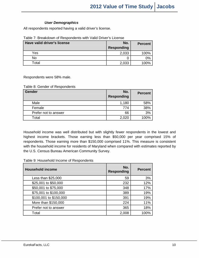
2012 Value of Time Study Jacobs
EurekaFacts, LLC 10
User Demographics All respondents reported having a valid driver’s license. Table 7: Breakdown of Respondents with Valid Driver’s License Have valid driver's license No.
Responding Percent
Yes 2,033 100% No 0 0% Total 2,033 100%
Respondents were 58% male. Table 8: Gender of Respondents Gender No.
Responding Percent
Male 1,180 58% Female 774 38% Prefer not to answer 66 3% Total 2,020 100%
Household income was well distributed but with slightly fewer respondents in the lowest and highest income brackets. Those earning less than $50,000 per year comprised 15% of respondents. Those earning more than $150,000 comprised 11%. This measure is consistent with the household income for residents of Maryland when compared with estimates reported by the U.S. Census Bureau American Community Survey. Table 9: Household Income of Respondents
Household income No.
Responding Percent
Less than $25,000 59 3% $25,001 to $50,000 232 12% $50,001 to $75,000 348 17% $75,001 to $100,000 389 19% $100,001 to $150,000 391 19% More than $150,000 224 11%
Prefer not to answer 365 18%
Total 2,008 100%
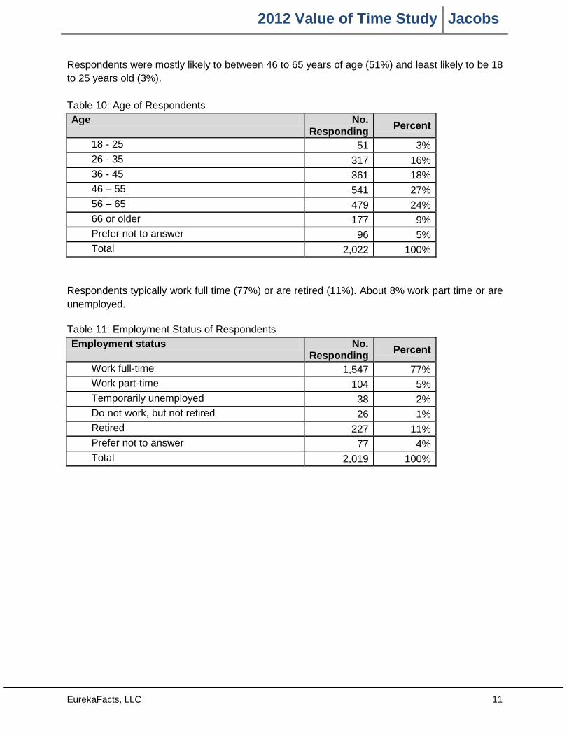
2012 Value of Time Study Jacobs
EurekaFacts, LLC 11
Respondents were mostly likely to between 46 to 65 years of age (51%) and least likely to be 18 to 25 years old (3%). Table 10: Age of Respondents Age No.
Responding Percent
18 - 25 51 3% 26 - 35 317 16% 36 - 45 361 18% 46 – 55 541 27% 56 – 65 479 24% 66 or older 177 9% Prefer not to answer 96 5% Total 2,022 100%
Respondents typically work full time (77%) or are retired (11%). About 8% work part time or are unemployed. Table 11: Employment Status of Respondents
Employment status No. Responding
Percent
Work full-time 1,547 77% Work part-time 104 5% Temporarily unemployed 38 2% Do not work, but not retired 26 1% Retired 227 11% Prefer not to answer 77 4% Total 2,019 100%
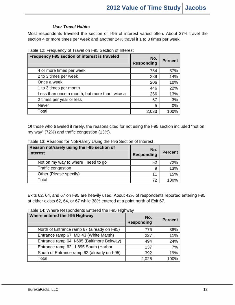
2012 Value of Time Study Jacobs
EurekaFacts, LLC 12
User Travel Habits Most respondents traveled the section of I-95 of interest varied often. About 37% travel the section 4 or more times per week and another 24% travel it 1 to 3 times per week. Table 12: Frequency of Travel on I-95 Section of Interest
Frequency I-95 section of interest is traveled
No. Responding
Percent
4 or more times per week 754 37% 2 to 3 times per week 289 14% Once a week 206 10% 1 to 3 times per month 446 22% Less than once a month, but more than twice a
266 13%
2 times per year or less 67 3% Never 5 0% Total 2,033 100%
Of those who traveled it rarely, the reasons cited for not using the I-95 section included “not on my way” (72%) and traffic congestion (13%).
Table 13: Reasons for Not/Rarely Using the I-95 Section of Interest
Reason not/rarely using the I-95 section of interest
No. Responding
Percent
Not on my way to where I need to go 52 72% Traffic congestion 9 13% Other (Please specify) 11 15% Total 72 100%
Exits 62, 64, and 67 on I-95 are heavily used. About 42% of respondents reported entering I-95 at either exists 62, 64, or 67 while 38% entered at a point north of Exit 67.
Table 14: Where Respondents Entered the I-95 Highway Where entered the I-95 Highway No.
Responding Percent
North of Entrance ramp 67 (already on I-95) 776 38% Entrance ramp 67 MD 43 (White Marsh)
227 11%
Entrance ramp 64 I-695 (Baltimore Beltway) 494 24% Entrance ramp 62, I-895 South (Harbor
137 7%
South of Entrance ramp 62 (already on I-95) 392 19% Total 2,026 100%
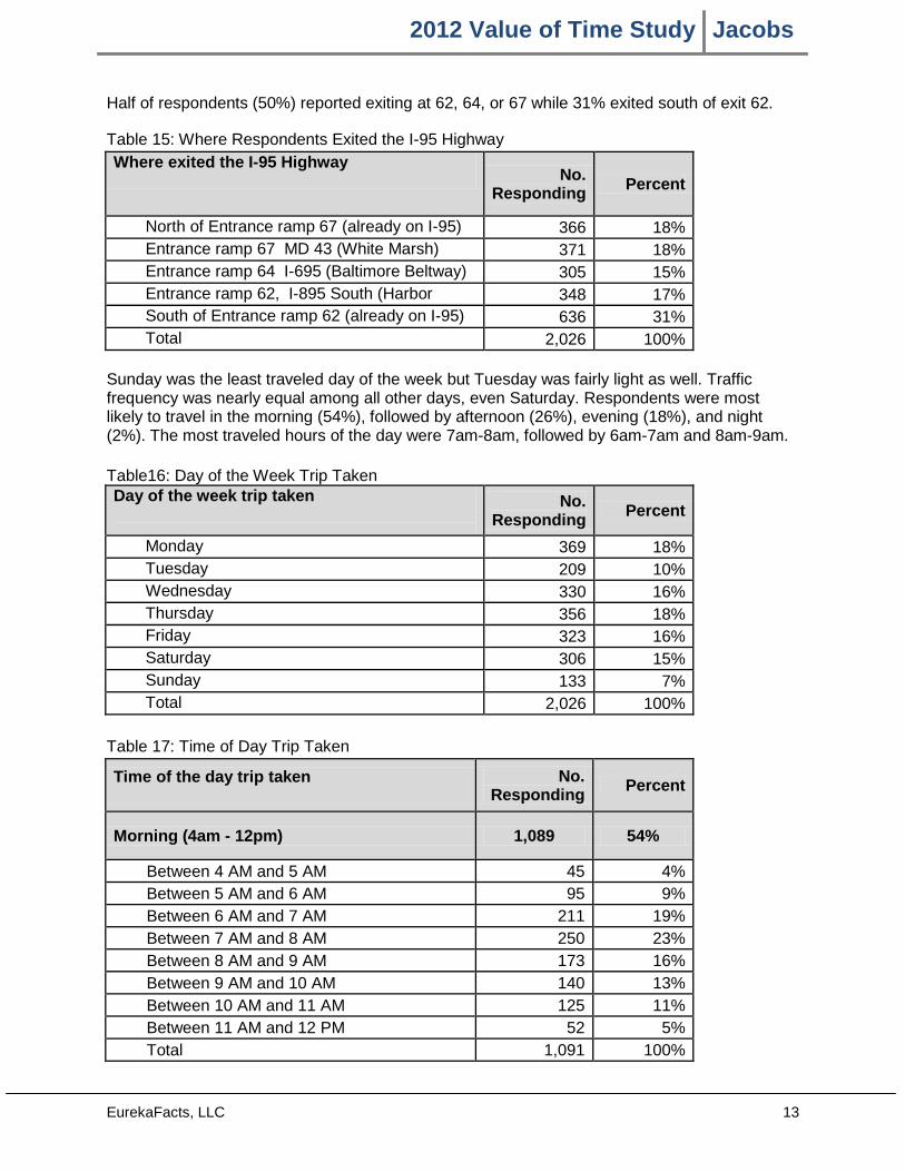
2012 Value of Time Study Jacobs
EurekaFacts, LLC 13
Half of respondents (50%) reported exiting at 62, 64, or 67 while 31% exited south of exit 62.
Table 15: Where Respondents Exited the I-95 Highway Where exited the I-95 Highway
No. Responding
Percent
North of Entrance ramp 67 (already on I-95) 366 18% Entrance ramp 67 MD 43 (White Marsh)
371 18%
Entrance ramp 64 I-695 (Baltimore Beltway) 305 15% Entrance ramp 62, I-895 South (Harbor
348 17%
South of Entrance ramp 62 (already on I-95) 636 31% Total 2,026 100%
Sunday was the least traveled day of the week but Tuesday was fairly light as well. Traffic frequency was nearly equal among all other days, even Saturday. Respondents were most likely to travel in the morning (54%), followed by afternoon (26%), evening (18%), and night (2%). The most traveled hours of the day were 7am-8am, followed by 6am-7am and 8am-9am. Table16: Day of the Week Trip Taken Day of the week trip taken
No. Responding
Percent
Monday 369 18% Tuesday 209 10% Wednesday 330 16% Thursday 356 18% Friday 323 16% Saturday 306 15% Sunday 133 7% Total 2,026 100%
Table 17: Time of Day Trip Taken
Time of the day trip taken No. Responding
Percent
Morning (4am - 12pm) 1,089 54%
Between 4 AM and 5 AM 45 4% Between 5 AM and 6 AM 95 9% Between 6 AM and 7 AM 211 19% Between 7 AM and 8 AM 250 23% Between 8 AM and 9 AM 173 16% Between 9 AM and 10 AM 140 13% Between 10 AM and 11 AM 125 11% Between 11 AM and 12 PM 52 5% Total 1,091 100%
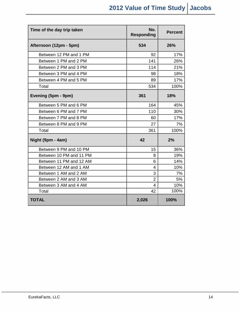
2012 Value of Time Study Jacobs
EurekaFacts, LLC 14
Time of the day trip taken No. Responding
Percent
Afternoon (12pm - 5pm) 534 26%
Between 12 PM and 1 PM 92 17%
Between 1 PM and 2 PM 141 26%
Between 2 PM and 3 PM 114 21%
Between 3 PM and 4 PM 98 18%
Between 4 PM and 5 PM 89 17%
Total 534 100%
Evening (5pm - 9pm) 361 18%
Between 5 PM and 6 PM 164 45%
Between 6 PM and 7 PM 110 30%
Between 7 PM and 8 PM 60 17%
Between 8 PM and 9 PM 27 7%
Total 361 100%
Night (9pm - 4am) 42 2%
Between 9 PM and 10 PM 15 36% Between 10 PM and 11 PM 8 19% Between 11 PM and 12 AM 6 14% Between 12 AM and 1 AM 4 10% Between 1 AM and 2 AM 3 7% Between 2 AM and 3 AM 2 5% Between 3 AM and 4 AM 4 10% Total 42 100%
TOTAL 2,026 100%
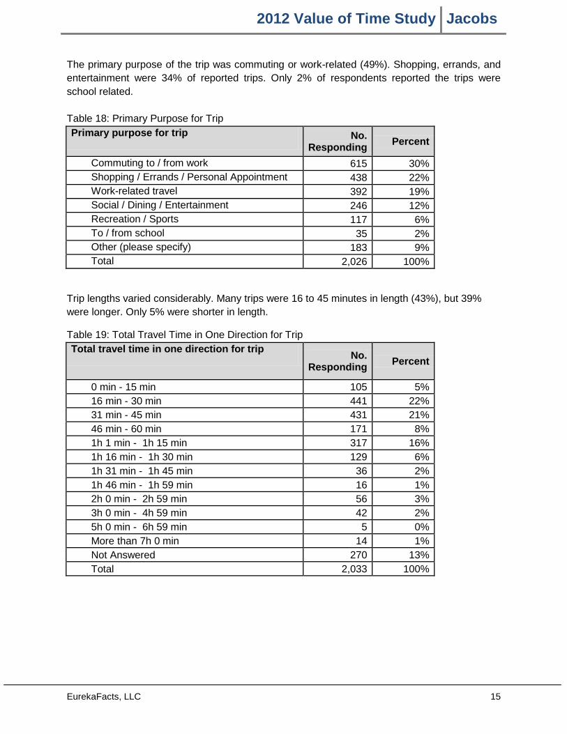
2012 Value of Time Study Jacobs
EurekaFacts, LLC 15
The primary purpose of the trip was commuting or work-related (49%). Shopping, errands, and entertainment were 34% of reported trips. Only 2% of respondents reported the trips were school related. Table 18: Primary Purpose for Trip
Primary purpose for trip No. Responding
Percent
Commuting to / from work 615 30% Shopping / Errands / Personal Appointment 438 22% Work-related travel 392 19% Social / Dining / Entertainment 246 12% Recreation / Sports 117 6% To / from school 35 2% Other (please specify) 183 9% Total 2,026 100%
Trip lengths varied considerably. Many trips were 16 to 45 minutes in length (43%), but 39% were longer. Only 5% were shorter in length.
Table 19: Total Travel Time in One Direction for Trip Total travel time in one direction for trip
No. Responding
Percent
0 min - 15 min 105 5% 16 min - 30 min 441 22% 31 min - 45 min 431 21% 46 min - 60 min 171 8% 1h 1 min - 1h 15 min 317 16% 1h 16 min - 1h 30 min 129 6% 1h 31 min - 1h 45 min 36 2% 1h 46 min - 1h 59 min 16 1% 2h 0 min - 2h 59 min 56 3% 3h 0 min - 4h 59 min 42 2% 5h 0 min - 6h 59 min 5 0% More than 7h 0 min 14 1% Not Answered 270 13% Total 2,033 100%
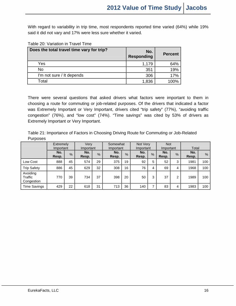
2012 Value of Time Study Jacobs
EurekaFacts, LLC 16
With regard to variability in trip time, most respondents reported time varied (64%) while 19% said it did not vary and 17% were less sure whether it varied. Table 20: Variation in Travel Time
Does the total travel time vary for trip? No. Responding
Percent
Yes 1,179 64% No 351 19% I'm not sure / It depends 306 17% Total 1,836 100%
There were several questions that asked drivers what factors were important to them in choosing a route for commuting or job-related purposes. Of the drivers that indicated a factor was Extremely Important or Very Important, drivers cited “trip safety” (77%), “avoiding traffic congestion” (76%), and “low cost” (74%). “Time savings” was cited by 53% of drivers as Extremely Important or Very Important. Table 21: Importance of Factors in Choosing Driving Route for Commuting or Job-Related Purposes
Extremely Important
Very Important
Somewhat Important
Not Very Important
Not Important Total
No. Resp.
% No.
Resp. %
No. Resp.
% No.
Resp. %
No. Resp.
% No.
Resp. %
Low Cost 888 45 574 29 375 19 92 5 52 3 1981 100
Trip Safety 886 45 629 32 308 16 76 4 69 4 1968 100
Avoiding Traffic Congestion
770 39 734 37 398 20 50 3 37 2 1989 100
Time Savings 429 22 618 31 713 36 140 7 83 4 1983 100
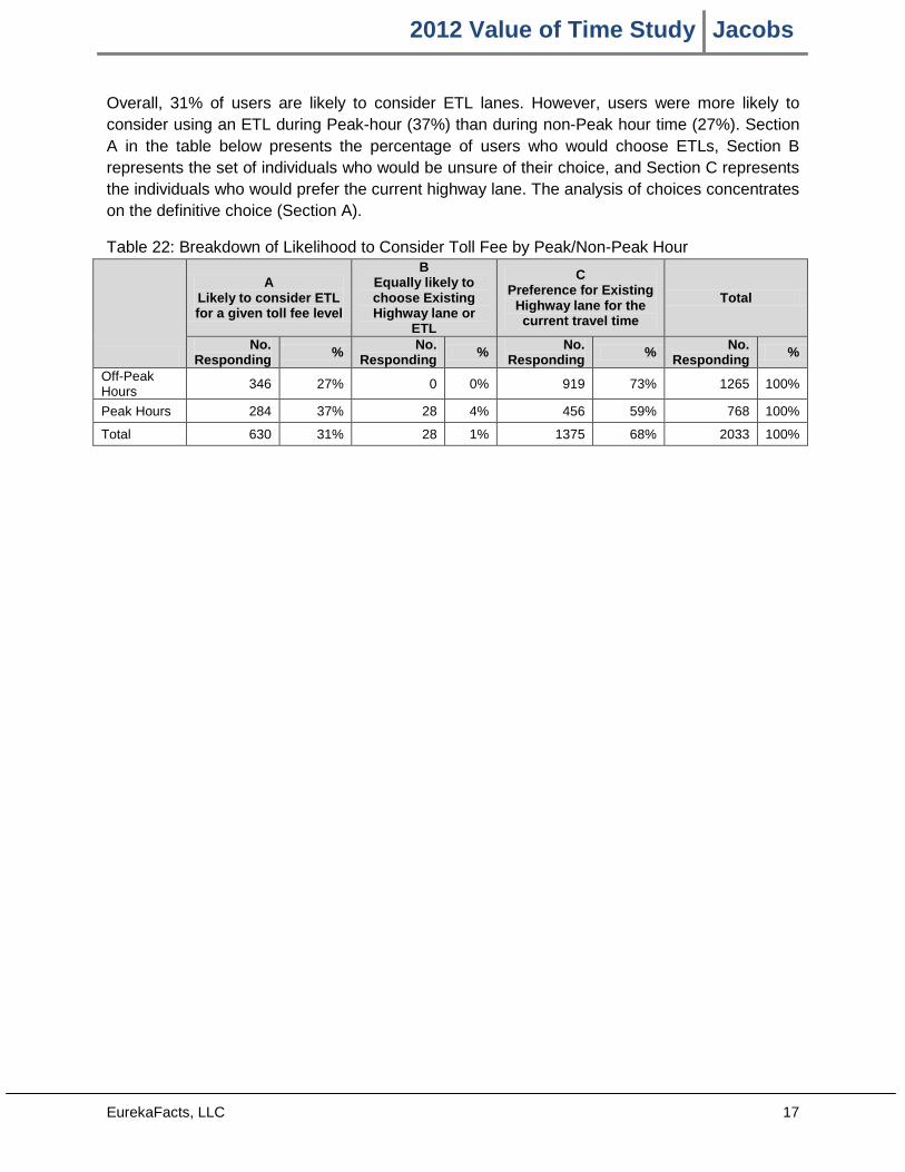
2012 Value of Time Study Jacobs
EurekaFacts, LLC 17
Overall, 31% of users are likely to consider ETL lanes. However, users were more likely to consider using an ETL during Peak-hour (37%) than during non-Peak hour time (27%). Section A in the table below presents the percentage of users who would choose ETLs, Section B represents the set of individuals who would be unsure of their choice, and Section C represents the individuals who would prefer the current highway lane. The analysis of choices concentrates on the definitive choice (Section A).
Table 22: Breakdown of Likelihood to Consider Toll Fee by Peak/Non-Peak Hour
A Likely to consider ETL for a given toll fee level
B Equally likely to choose Existing Highway lane or
ETL
C Preference for Existing
Highway lane for the current travel time
Total
No. Responding
% No.
Responding %
No. Responding
% No.
Responding %
Off-Peak Hours
346 27% 0 0% 919 73% 1265 100%
Peak Hours 284 37% 28 4% 456 59% 768 100%
Total 630 31% 28 1% 1375 68% 2033 100%
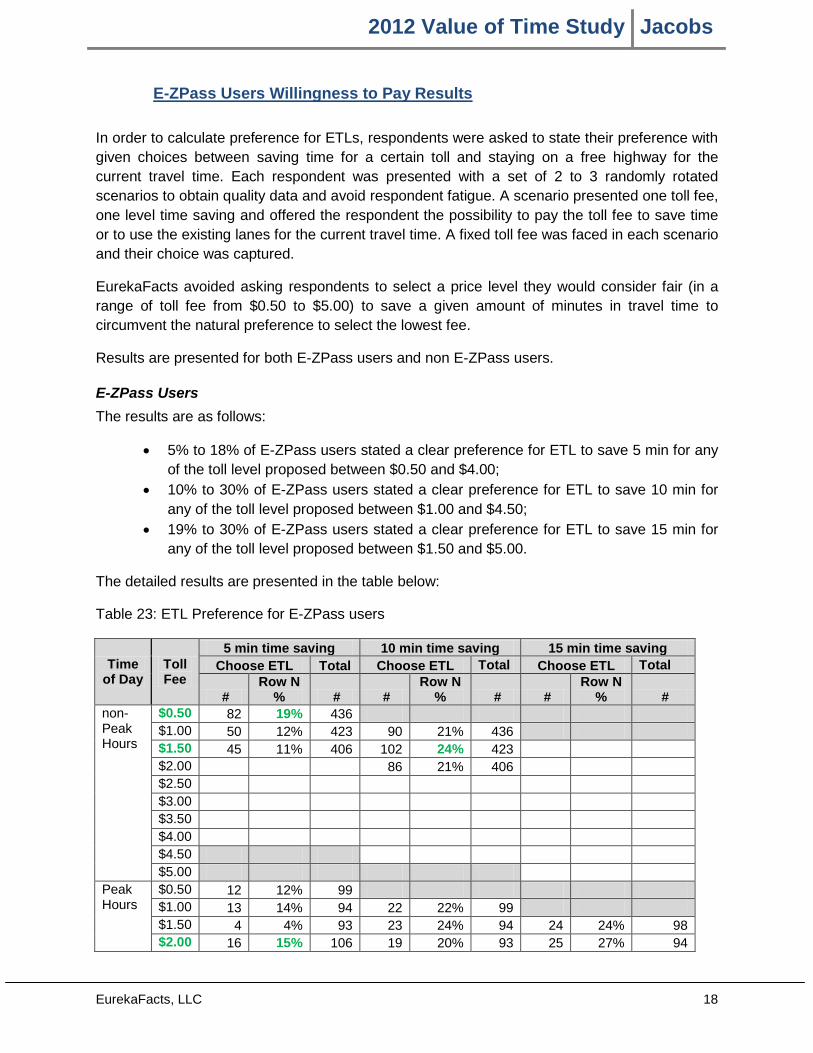
2012 Value of Time Study Jacobs
EurekaFacts, LLC 18
E-ZPass Users Willingness to Pay Results
In order to calculate preference for ETLs, respondents were asked to state their preference with given choices between saving time for a certain toll and staying on a free highway for the current travel time. Each respondent was presented with a set of 2 to 3 randomly rotated scenarios to obtain quality data and avoid respondent fatigue. A scenario presented one toll fee, one level time saving and offered the respondent the possibility to pay the toll fee to save time or to use the existing lanes for the current travel time. A fixed toll fee was faced in each scenario and their choice was captured.
EurekaFacts avoided asking respondents to select a price level they would consider fair (in a range of toll fee from $0.50 to $5.00) to save a given amount of minutes in travel time to circumvent the natural preference to select the lowest fee.
Results are presented for both E-ZPass users and non E-ZPass users.
E-ZPass Users The results are as follows:
• 5% to 18% of E-ZPass users stated a clear preference for ETL to save 5 min for any of the toll level proposed between $0.50 and $4.00;
• 10% to 30% of E-ZPass users stated a clear preference for ETL to save 10 min for any of the toll level proposed between $1.00 and $4.50;
• 19% to 30% of E-ZPass users stated a clear preference for ETL to save 15 min for any of the toll level proposed between $1.50 and $5.00.
The detailed results are presented in the table below:
Table 23: ETL Preference for E-ZPass users
Time of Day
Toll Fee
5 min time saving 10 min time saving 15 min time saving Choose ETL Total Choose ETL Total Choose ETL Total
# Row N
% # # Row N
% # # Row N
% # non-Peak Hours
$0.50 82 19% 436 $1.00 50 12% 423 90 21% 436 $1.50 45 11% 406 102 24% 423 $2.00 86 21% 406 $2.50 $3.00 $3.50 $4.00 $4.50 $5.00
Peak Hours
$0.50 12 12% 99 $1.00 13 14% 94 22 22% 99 $1.50 4 4% 93 23 24% 94 24 24% 98 $2.00 16 15% 106 19 20% 93 25 27% 94
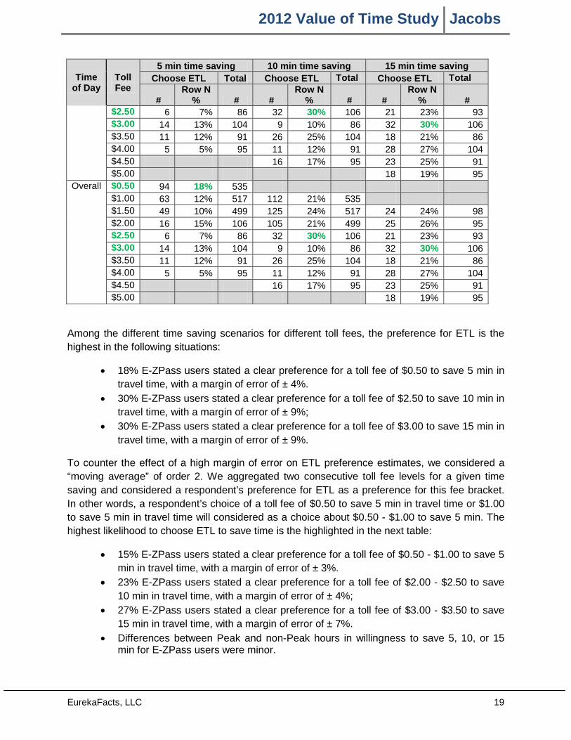
2012 Value of Time Study Jacobs
EurekaFacts, LLC 19
Time of Day
Toll Fee
5 min time saving 10 min time saving 15 min time saving Choose ETL Total Choose ETL Total Choose ETL Total
# Row N
% # # Row N
% # # Row N
% # $2.50 6 7% 86 32 30% 106 21 23% 93 $3.00 14 13% 104 9 10% 86 32 30% 106 $3.50 11 12% 91 26 25% 104 18 21% 86 $4.00 5 5% 95 11 12% 91 28 27% 104 $4.50 16 17% 95 23 25% 91 $5.00 18 19% 95
Overall $0.50 94 18% 535 $1.00 63 12% 517 112 21% 535 $1.50 49 10% 499 125 24% 517 24 24% 98 $2.00 16 15% 106 105 21% 499 25 26% 95 $2.50 6 7% 86 32 30% 106 21 23% 93 $3.00 14 13% 104 9 10% 86 32 30% 106 $3.50 11 12% 91 26 25% 104 18 21% 86 $4.00 5 5% 95 11 12% 91 28 27% 104 $4.50 16 17% 95 23 25% 91 $5.00 18 19% 95
Among the different time saving scenarios for different toll fees, the preference for ETL is the highest in the following situations:
• 18% E-ZPass users stated a clear preference for a toll fee of $0.50 to save 5 min in travel time, with a margin of error of ± 4%.
• 30% E-ZPass users stated a clear preference for a toll fee of $2.50 to save 10 min in travel time, with a margin of error of ± 9%;
• 30% E-ZPass users stated a clear preference for a toll fee of $3.00 to save 15 min in travel time, with a margin of error of ± 9%.
To counter the effect of a high margin of error on ETL preference estimates, we considered a “moving average” of order 2. We aggregated two consecutive toll fee levels for a given time saving and considered a respondent’s preference for ETL as a preference for this fee bracket. In other words, a respondent’s choice of a toll fee of $0.50 to save 5 min in travel time or $1.00 to save 5 min in travel time will considered as a choice about $0.50 - $1.00 to save 5 min. The highest likelihood to choose ETL to save time is the highlighted in the next table:
• 15% E-ZPass users stated a clear preference for a toll fee of $0.50 - $1.00 to save 5 min in travel time, with a margin of error of ± 3%.
• 23% E-ZPass users stated a clear preference for a toll fee of $2.00 - $2.50 to save 10 min in travel time, with a margin of error of ± 4%;
• 27% E-ZPass users stated a clear preference for a toll fee of $3.00 - $3.50 to save 15 min in travel time, with a margin of error of ± 7%.
• Differences between Peak and non-Peak hours in willingness to save 5, 10, or 15 min for E-ZPass users were minor.
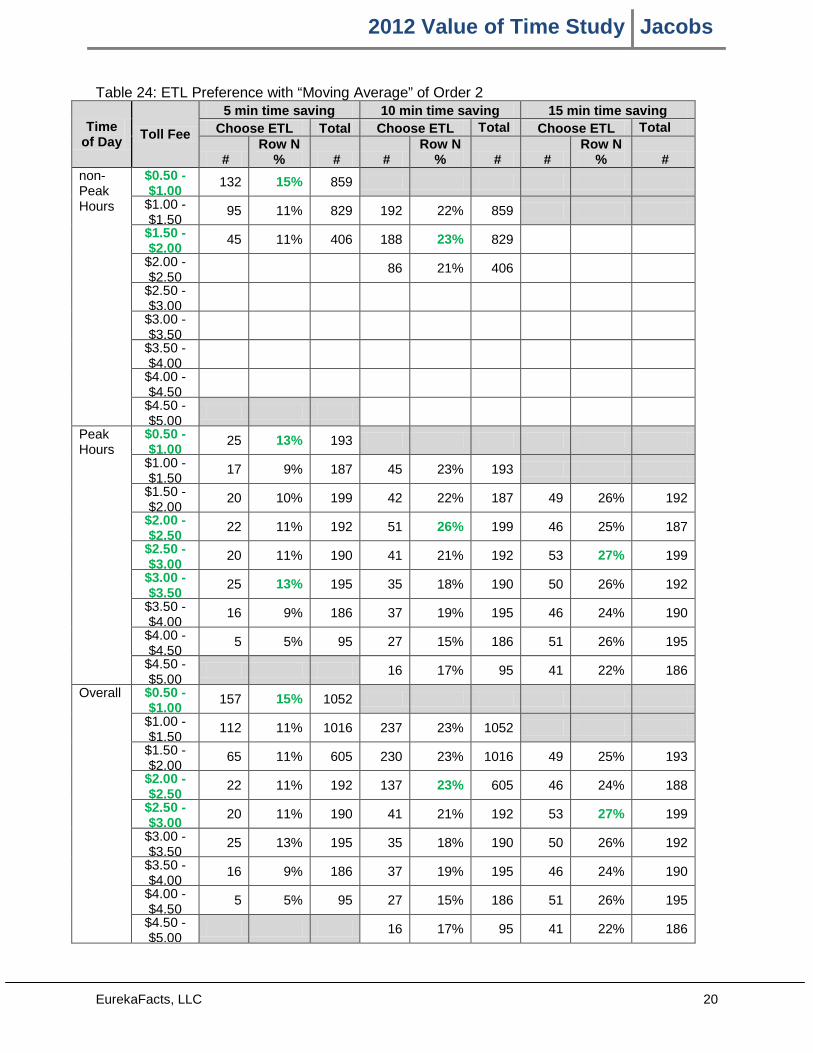
2012 Value of Time Study Jacobs
EurekaFacts, LLC 20
Table 24: ETL Preference with “Moving Average” of Order 2
Time of Day
Toll Fee
5 min time saving 10 min time saving 15 min time saving Choose ETL Total Choose ETL Total Choose ETL Total
# Row N
% # # Row N
% # # Row N
% # non-Peak Hours
$0.50 - $1.00
132 15% 859
$1.00 - $1.50
95 11% 829 192 22% 859
$1.50 - $2.00
45 11% 406 188 23% 829
$2.00 - $2.50
86 21% 406
$2.50 - $3.00
$3.00 - $3.50
$3.50 - $4.00
$4.00 - $4.50
$4.50 - $5.00
Peak Hours
$0.50 - $1.00
25 13% 193
$1.00 - $1.50
17 9% 187 45 23% 193
$1.50 - $2.00
20 10% 199 42 22% 187 49 26% 192
$2.00 - $2.50
22 11% 192 51 26% 199 46 25% 187
$2.50 - $3.00
20 11% 190 41 21% 192 53 27% 199
$3.00 - $3.50
25 13% 195 35 18% 190 50 26% 192
$3.50 - $4.00
16 9% 186 37 19% 195 46 24% 190
$4.00 - $4.50
5 5% 95 27 15% 186 51 26% 195
$4.50 - $5.00
16 17% 95 41 22% 186
Overall $0.50 - $1.00
157 15% 1052
$1.00 - $1.50
112 11% 1016 237 23% 1052
$1.50 - $2.00
65 11% 605 230 23% 1016 49 25% 193
$2.00 - $2.50
22 11% 192 137 23% 605 46 24% 188
$2.50 - $3.00
20 11% 190 41 21% 192 53 27% 199
$3.00 - $3.50
25 13% 195 35 18% 190 50 26% 192
$3.50 - $4.00
16 9% 186 37 19% 195 46 24% 190
$4.00 - $4.50
5 5% 95 27 15% 186 51 26% 195
$4.50 - $5.00
16 17% 95 41 22% 186

2012 Value of Time Study Jacobs
EurekaFacts, LLC 21
Overall, the empirical likelihood of E-ZPass users are likely to consider ETL for any given toll fee level at any time saving was 31%. A number of factors influence the likelihood that a respondent will chose ETL:
• This percentage increases up to 33% for those who travel on the I-95 Highway section between the I-95/I-895 merge and MD 43/White Marsh Boulevard in either direction 4 times per week or more, and falls to 28% for those who travel less than once a week in this I-95 section.
• The primary purpose of the commute seems to influence ETL preference as well. Respondents commuting to/from work, on a work-related travel or for social/dining/entertainment have an overall preference above 33% while those commuting for other purposes have a preference below 31%.
• Concern for time saving, traffic congestion, low cost and trip safety also influence the likelihood to use ETL.
o 47% of those who consider time saving extremely important are likely to consider ETL.
o 37% of those who consider traffic congestion extremely important are likely to consider ETL.
o 31% of those who consider the trip safety extremely important are likely to consider ETL.
o 24% of those who consider the cost extremely important are likely to consider ETL.
• With regard for household income, 37% of respondents with a household above $150,000 are likely to consider ETL compared to 32% of respondents with a household income below $50,000.
• When age is considered, 42% of those 18 to 35 years old are likely to consider ETL compared to 26% of respondents 56 years and older.
• Regarding gender, 32% of males would consider ETL versus 30% of females.
In some cases, respondents overwhelmingly belong to one group casting doubt on the robustness of any comparison with other categories of the group: about 94% of respondents drive a passenger car, SUV or pick-up truck, 85% drive private vehicles and 75% work full-time.
Non E-ZPass Users Tables 25 and 26 present the results for non E-ZPass users; however, there is insufficient data to make conclusive inferences. Because the counts per cell are small, the margins of error are quite high. Readers are cautioned not to draw erroneous conclusions.
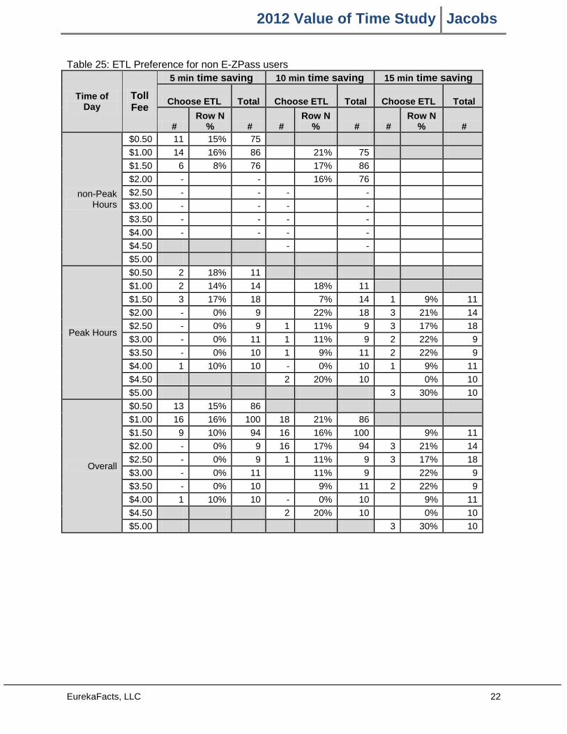
2012 Value of Time Study Jacobs
EurekaFacts, LLC 22
Table 25: ETL Preference for non E-ZPass users
Time of Day
Toll Fee
5 min time saving 10 min time saving 15 min time saving
Choose ETL Total Choose ETL Total Choose ETL Total
# Row N
% # # Row N
% # # Row N
% #
non-Peak Hours
$0.50 11 15% 75
$1.00 14 16% 86
21% 75
$1.50 6 8% 76
17% 86
$2.00 - -
16% 76
$2.50 - - - -
$3.00 - - - -
$3.50 - - - -
$4.00 - - - -
$4.50 - -
$5.00
Peak Hours
$0.50 2 18% 11
$1.00 2 14% 14
18% 11
$1.50 3 17% 18
7% 14 1 9% 11
$2.00 - 0% 9
22% 18 3 21% 14
$2.50 - 0% 9 1 11% 9 3 17% 18
$3.00 - 0% 11 1 11% 9 2 22% 9
$3.50 - 0% 10 1 9% 11 2 22% 9
$4.00 1 10% 10 - 0% 10 1 9% 11
$4.50 2 20% 10
0% 10
$5.00 3 30% 10
Overall
$0.50 13 15% 86
$1.00 16 16% 100 18 21% 86
$1.50 9 10% 94 16 16% 100
9% 11
$2.00 - 0% 9 16 17% 94 3 21% 14
$2.50 - 0% 9 1 11% 9 3 17% 18
$3.00 - 0% 11
11% 9
22% 9
$3.50 - 0% 10
9% 11 2 22% 9
$4.00 1 10% 10 - 0% 10
9% 11
$4.50 2 20% 10
0% 10
$5.00 3 30% 10

2012 Value of Time Study Jacobs
EurekaFacts, LLC 23
Table 26: ETL Preference with “Moving Average” of Order 2
Time of Day
Toll Fee
5 min time saving 10 min time saving 15 min time saving
Choose ETL Total Choose ETL Total Choose ETL Total
# Row N
% # # Row N
% # # Row N
% # non-Peak Hours
$0.50 - $1.00
25 16% 161
$1.00 - $1.50
20 12% 162 31 19% 161
$1.50 - $2.00
6 8% 76 27 17% 162
$2.00 - $2.50
- - 12 16% 76
$2.50 - $3.00
- - - -
$3.00 - $3.50
- - - -
$3.50 - $4.00
- - - -
$4.00 - $4.50
- - - -
$4.50 - $5.00
- -
Peak Hours
$0.50 - $1.00
4 16% 25
$1.00 - $1.50
5 16% 32 3 12% 25
$1.50 - $2.00
3 11% 27 5 16% 32 4 16% 25
$2.00 - $2.50
- 0% 18 5
19% 27 6 19% 32
$2.50 - $3.00
- 0% 20 2 11% 18 5 19% 27
$3.00 - $3.50
- 0% 21 2 10% 20 4
22% 18
$3.50 - $4.00
1 5% 20 1 5% 21 3
15% 20
$4.00 - $4.50
1 10% 10 2 10% 20 1 5% 21
$4.50 - $5.00
2 20% 10 3 15% 20
Overall $0.50 - $1.00
29 16% 186
$1.00 - $1.50
25 13% 194 34 18% 186
$1.50 - $2.00
9 9% 103 32 16% 194 4 16% 25
$2.00 - $2.50
- 0% 18 17 17% 103 6 19% 32
$2.50 - $3.00
- 0% 20 2 11% 18 5 19% 27
$3.00 - $3.50
- 0% 21 2 10% 20 4 22% 18
$3.50 - $4.00
1 5% 20 1 5% 21 3 15% 20
$4.00 - $4.50
1 10% 10 2 10% 20 1 5% 21
$4.50 - $5.00
2 20% 10 3 15% 20
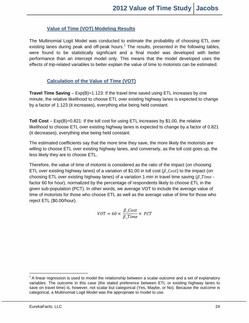
2012 Value of Time Study Jacobs
EurekaFacts, LLC 24
Value of Time (VOT) Modeling Results The Multinomial Logit Model was conducted to estimate the probability of choosing ETL over existing lanes during peak and off-peak hours.1 The results, presented in the following tables, were found to be statistically significant and a final model was developed with better performance than an intercept model only. This means that the model developed uses the effects of trip-related variables to better explain the value of time to motorists can be estimated.
Calculation of the Value of Time (VOT) Travel Time Saving – Exp(B)=1.123: If the travel time saved using ETL increases by one minute, the relative likelihood to choose ETL over existing highway lanes is expected to change by a factor of 1.123 (it increases), everything else being held constant.
Toll Cost – Exp(B)=0.821: If the toll cost for using ETL increases by $1.00, the relative likelihood to choose ETL over existing highway lanes is expected to change by a factor of 0.821 (it decreases), everything else being held constant.
The estimated coefficients say that the more time they save, the more likely the motorists are willing to choose ETL over existing highway lanes, and conversely, as the toll cost goes up, the less likely they are to choose ETL.
Therefore, the value of time of motorist is considered as the ratio of the impact (on choosing ETL over existing highway lanes) of a variation of $1.00 in toll cost (𝛽_𝐶𝑜𝑠𝑡) to the impact (on choosing ETL over existing highway lanes) of a variation 1 min in travel time saving (𝛽_𝑇𝑖𝑚𝑒 - factor 60 for hour), normalized by the percentage of respondents likely to choose ETL in the given sub-population (PCT). In other words, we average VOT to include the average value of time of motorists for those who choose ETL as well as the average value of time for those who reject ETL ($0.00/hour).
𝑉𝑂𝑇 = 60 × 𝛽_𝐶𝑜𝑠𝑡𝛽_𝑇𝑖𝑚𝑒
× 𝑃𝐶𝑇
1 A linear regression is used to model the relationship between a scalar outcome and a set of explanatory variables. The outcome in this case (the stated preference between ETL or existing highway lanes to save on travel time) is, however, not scalar but categorical (Yes, Maybe, or No). Because the outcome is categorical, a Multinomial Logit Model was the appropriate to model to use.
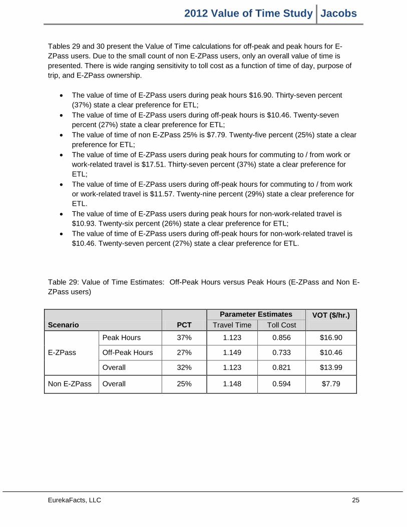
2012 Value of Time Study Jacobs
EurekaFacts, LLC 25
Tables 29 and 30 present the Value of Time calculations for off-peak and peak hours for E-ZPass users. Due to the small count of non E-ZPass users, only an overall value of time is presented. There is wide ranging sensitivity to toll cost as a function of time of day, purpose of trip, and E-ZPass ownership.
• The value of time of E-ZPass users during peak hours $16.90. Thirty-seven percent (37%) state a clear preference for ETL;
• The value of time of E-ZPass users during off-peak hours is $10.46. Twenty-seven percent (27%) state a clear preference for ETL;
• The value of time of non E-ZPass 25% is $7.79. Twenty-five percent (25%) state a clear preference for ETL;
• The value of time of E-ZPass users during peak hours for commuting to / from work or work-related travel is $17.51. Thirty-seven percent (37%) state a clear preference for ETL;
• The value of time of E-ZPass users during off-peak hours for commuting to / from work or work-related travel is $11.57. Twenty-nine percent (29%) state a clear preference for ETL.
• The value of time of E-ZPass users during peak hours for non-work-related travel is $10.93. Twenty-six percent (26%) state a clear preference for ETL;
• The value of time of E-ZPass users during off-peak hours for non-work-related travel is $10.46. Twenty-seven percent (27%) state a clear preference for ETL.
Table 29: Value of Time Estimates: Off-Peak Hours versus Peak Hours (E-ZPass and Non E-ZPass users)
Scenario PCT
Parameter Estimates VOT ($/hr.) Travel Time Toll Cost
E-ZPass
Peak Hours 37% 1.123 0.856 $16.90
Off-Peak Hours 27% 1.149 0.733 $10.46
Overall 32% 1.123 0.821 $13.99
Non E-ZPass Overall 25% 1.148 0.594 $7.79
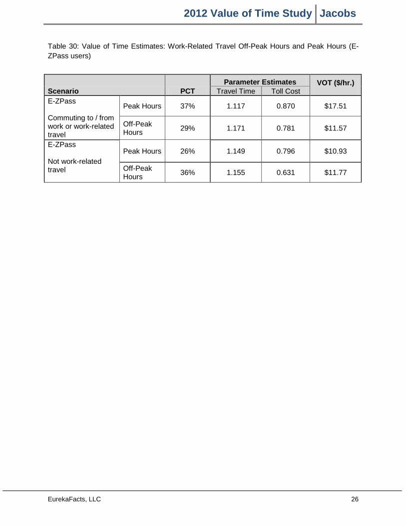
2012 Value of Time Study Jacobs
EurekaFacts, LLC 26
Table 30: Value of Time Estimates: Work-Related Travel Off-Peak Hours and Peak Hours (E-ZPass users)
Scenario PCT Parameter Estimates VOT ($/hr.)
Travel Time Toll Cost E-ZPass Commuting to / from work or work-related travel
Peak Hours 37% 1.117 0.870 $17.51
Off-Peak Hours
29% 1.171 0.781 $11.57
E-ZPass Not work-related travel
Peak Hours 26% 1.149 0.796 $10.93
Off-Peak Hours
36% 1.155 0.631 $11.77

2012 Value of Time Study Jacobs
EurekaFacts, LLC 27
Table 31 to Table 36 present the parameter estimates for ETL preference.
• Tables 31 to 34 present a different travel scenario for E-ZPass users (e.g., peak hours versus off-peak hours, work or work-related travel versus non work related travel).
• Table 35 presents E-ZPass users overall.
• Table 36 presents non E-ZPass users overall. Notes: Everything else held constant
1. The positive coefficient (column B) of the travel time savings indicates that the likelihood to choose ETL over existing highway lanes increases when travel time savings increases.
2. The negative coefficient (column B) of the toll cost indicates that the likelihood to choose ETL over existing highway lanes decreases
when the toll cost increases.
3. Sig. (column F) indicates the level of significance of the coefficient (in column B) compared to 0.
4. Exp(B) (column G) indicates an increased likelihood when greater than 1 and a decreased likelihood when less than 1.
5. Travel time saving and toll cost are considered continuous.

2012 Value of Time Study Jacobs
EurekaFacts, LLC 28
Table 31: Parameter Estimates: Commuting To / From Work or Work-Related Travel - Peak Hours (E-ZPass users)
Choicea
B Std. Error Wald df Sig. Exp(B)
95% Confidence Interval for Exp(B)
I would choose the ETL Lower Bound
Upper Bound
Intercept -4.131 1.270 10.578 1 .001
Travel Time Saving .111 .020 30.648 1 .000 1.117 1.074 1.162
Toll Cost -.139 .068 4.184 1 .041 .870 .761 .994
Gender: Male .369 .163 5.088 1 .024 1.446 1.049 1.991
Gender: Female 0b 0
HH Income: Less than $50,000 -.322 .289 1.246 1 .264 .725 .412 1.276
HH Income: $50,001 to $75,000 -.961 .268 12.915 1 .000 .382 .226 .646
HH Income: $75,001 to $100,000 -.210 .224 .883 1 .347 .810 .522 1.257
HH Income: $100,001 to $150,000 -.153 .226 .455 1 .500 .858 .551 1.338
HH Income: More than $150,000 0b 0
Age: 18 - 35 2.114 1.078 3.844 1 .050 8.280 1.001 68.504
Age: 36 - 45 2.161 1.075 4.040 1 .044 8.680 1.055 71.406
Age: 46 - 55 1.935 1.073 3.256 1 .071 6.926 .846 56.689
Age: 56 - 65 1.936 1.071 3.269 1 .071 6.934 .850 56.581
Age: 66 or older 0b 0
Employment Status: Work full-time -.260 .837 .096 1 .756 .771 .150 3.977
Employment Status: Work part-time or Unemployed, but not retired -.136 .909 .022 1 .881 .873 .147 5.188
Employment Status: Retired 0b 0
Vehicle Usage: Commercial or Mixed Commercial/Private .277 .181 2.348 1 .125 1.319 .926 1.880
Vehicle Usage: Private 0b 0
Travel frequency: 4 or more times per week .306 .393 .607 1 .436 1.358 .629 2.931
Travel frequency: 1 to 3 times per week .439 .418 1.102 1 .294 1.551 .684 3.517
Travel frequency: 1 to 3 times per month -.021 .478 .002 1 .965 .979 .383 2.500
Travel frequency: Less than once a month 0b 0
a. The reference category is: I would choose Existing Highway lane for the current travel time. b. This parameter is set to zero because it is redundant.
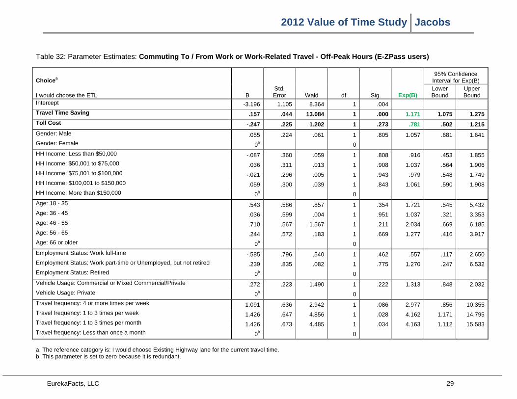
2012 Value of Time Study Jacobs
EurekaFacts, LLC 29
Table 32: Parameter Estimates: Commuting To / From Work or Work-Related Travel - Off-Peak Hours (E-ZPass users)
Choicea
B Std. Error Wald df Sig. Exp(B)
95% Confidence Interval for Exp(B)
I would choose the ETL Lower Bound
Upper Bound
Intercept -3.196 1.105 8.364 1 .004
Travel Time Saving .157 .044 13.084 1 .000 1.171 1.075 1.275
Toll Cost -.247 .225 1.202 1 .273 .781 .502 1.215
Gender: Male .055 .224 .061 1 .805 1.057 .681 1.641
Gender: Female 0b 0
HH Income: Less than $50,000 -.087 .360 .059 1 .808 .916 .453 1.855
HH Income: $50,001 to $75,000 .036 .311 .013 1 .908 1.037 .564 1.906
HH Income: $75,001 to $100,000 -.021 .296 .005 1 .943 .979 .548 1.749
HH Income: $100,001 to $150,000 .059 .300 .039 1 .843 1.061 .590 1.908
HH Income: More than $150,000 0b 0
Age: 18 - 35 .543 .586 .857 1 .354 1.721 .545 5.432
Age: 36 - 45 .036 .599 .004 1 .951 1.037 .321 3.353
Age: 46 - 55 .710 .567 1.567 1 .211 2.034 .669 6.185
Age: 56 - 65 .244 .572 .183 1 .669 1.277 .416 3.917
Age: 66 or older 0b 0
Employment Status: Work full-time -.585 .796 .540 1 .462 .557 .117 2.650
Employment Status: Work part-time or Unemployed, but not retired .239 .835 .082 1 .775 1.270 .247 6.532
Employment Status: Retired 0b 0
Vehicle Usage: Commercial or Mixed Commercial/Private .272 .223 1.490 1 .222 1.313 .848 2.032
Vehicle Usage: Private 0b 0
Travel frequency: 4 or more times per week 1.091 .636 2.942 1 .086 2.977 .856 10.355
Travel frequency: 1 to 3 times per week 1.426 .647 4.856 1 .028 4.162 1.171 14.795
Travel frequency: 1 to 3 times per month 1.426 .673 4.485 1 .034 4.163 1.112 15.583
Travel frequency: Less than once a month 0b 0
a. The reference category is: I would choose Existing Highway lane for the current travel time.
b. This parameter is set to zero because it is redundant.

2012 Value of Time Study Jacobs
EurekaFacts, LLC 30
Table 33: Parameter Estimates: Not Work Related Travel - Peak Hours (E-ZPass users)
Choicea
B Std. Error Wald df Sig. Exp(B)
95% Confidence Interval for Exp(B)
I would choose the ETL Lower Bound
Upper Bound
Intercept -2.700 .709 14.521 1 .000
Travel Time Saving .139 .030 21.164 1 .000 1.149 1.083 1.220
Toll Cost -.228 .099 5.282 1 .022 .796 .656 .967
Gender: Male -.030 .241 .016 1 .901 .970 .605 1.556
Gender: Female 0b 0
HH Income: Less than $50,000 .184 .391 .221 1 .639 1.202 .558 2.588
HH Income: $50,001 to $75,000 -.348 .389 .800 1 .371 .706 .329 1.513
HH Income: $75,001 to $100,000 -.950 .418 5.165 1 .023 .387 .170 .877
HH Income: $100,001 to $150,000 -.658 .397 2.746 1 .098 .518 .238 1.128
HH Income: More than $150,000 0b 0
Age: 18 - 35 1.664 .564 8.693 1 .003 5.279 1.747 15.952
Age: 36 - 45 .604 .573 1.110 1 .292 1.829 .595 5.626
Age: 46 - 55 1.492 .574 6.767 1 .009 4.448 1.445 13.695
Age: 56 - 65 .892 .484 3.398 1 .065 2.439 .945 6.294
Age: 66 or older 0b 0
Employment Status: Work full-time .098 .441 .050 1 .823 1.103 .465 2.618
Employment Status: Work part-time or Unemployed, but not retired .286 .485 .348 1 .555 1.331 .514 3.447
Employment Status: Retired 0b 0
Vehicle Usage: Commercial or Mixed Commercial/Private -.433 .597 .528 1 .467 .648 .201 2.087
Vehicle Usage: Private 0b 0
Travel frequency: 4 or more times per week .051 .465 .012 1 .912 1.053 .423 2.618
Travel frequency: 1 to 3 times per week -.344 .327 1.107 1 .293 .709 .374 1.345
Travel frequency: 1 to 3 times per month -.032 .325 .010 1 .921 .968 .512 1.830
Travel frequency: Less than once a month 0b 0
a. The reference category is: I would choose Existing Highway lane for the current travel time.
b. This parameter is set to zero because it is redundant.
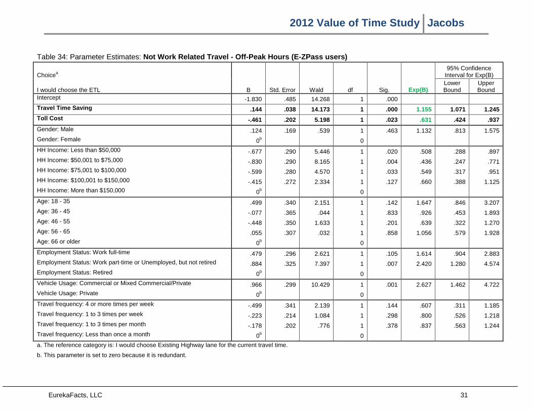
2012 Value of Time Study Jacobs
EurekaFacts, LLC 31
Table 34: Parameter Estimates: Not Work Related Travel - Off-Peak Hours (E-ZPass users)
Choicea
B Std. Error Wald df Sig. Exp(B)
95% Confidence Interval for Exp(B)
I would choose the ETL Lower Bound
Upper Bound
Intercept -1.830 .485 14.268 1 .000
Travel Time Saving .144 .038 14.173 1 .000 1.155 1.071 1.245
Toll Cost -.461 .202 5.198 1 .023 .631 .424 .937
Gender: Male .124 .169 .539 1 .463 1.132 .813 1.575
Gender: Female 0b 0
HH Income: Less than $50,000 -.677 .290 5.446 1 .020 .508 .288 .897
HH Income: $50,001 to $75,000 -.830 .290 8.165 1 .004 .436 .247 .771
HH Income: $75,001 to $100,000 -.599 .280 4.570 1 .033 .549 .317 .951
HH Income: $100,001 to $150,000 -.415 .272 2.334 1 .127 .660 .388 1.125
HH Income: More than $150,000 0b 0
Age: 18 - 35 .499 .340 2.151 1 .142 1.647 .846 3.207
Age: 36 - 45 -.077 .365 .044 1 .833 .926 .453 1.893
Age: 46 - 55 -.448 .350 1.633 1 .201 .639 .322 1.270
Age: 56 - 65 .055 .307 .032 1 .858 1.056 .579 1.928
Age: 66 or older 0b 0
Employment Status: Work full-time .479 .296 2.621 1 .105 1.614 .904 2.883
Employment Status: Work part-time or Unemployed, but not retired .884 .325 7.397 1 .007 2.420 1.280 4.574
Employment Status: Retired 0b 0
Vehicle Usage: Commercial or Mixed Commercial/Private .966 .299 10.429 1 .001 2.627 1.462 4.722
Vehicle Usage: Private 0b 0
Travel frequency: 4 or more times per week -.499 .341 2.139 1 .144 .607 .311 1.185
Travel frequency: 1 to 3 times per week -.223 .214 1.084 1 .298 .800 .526 1.218
Travel frequency: 1 to 3 times per month -.178 .202 .776 1 .378 .837 .563 1.244
Travel frequency: Less than once a month 0b 0
a. The reference category is: I would choose Existing Highway lane for the current travel time.
b. This parameter is set to zero because it is redundant.

2012 Value of Time Study Jacobs
EurekaFacts, LLC 32
Table 35: Parameter Estimates: E-ZPass users
Choicea
B Std. Error Wald df Sig. Exp(B)
95% Confidence Interval for Exp(B)
I would choose the ETL Lower Bound
Upper Bound
-2.536 .281 81.384 1 .000
Travel Time Saving .116 .014 70.624 1 .000 1.123 1.093 1.154
Toll Cost -.198 .043 21.584 1 .000 .821 .755 .892
Gender: Male .217 .092 5.604 1 .018 1.243 1.038 1.488
Gender: Female 0b 0
HH Income: Less than $50,000 -.286 .154 3.423 1 .064 .752 .555 1.017
HH Income: $50,001 to $75,000 -.530 .147 12.983 1 .000 .589 .441 .785
HH Income: $75,001 to $100,000 -.331 .138 5.732 1 .017 .718 .547 .942
HH Income: $100,001 to $150,000 -.265 .138 3.687 1 .055 .768 .586 1.006
HH Income: More than $150,000 0b 0
Age: 18 - 35 .789 .231 11.674 1 .001 2.201 1.400 3.460
Age: 36 - 45 .401 .234 2.924 1 .087 1.493 .943 2.364
Age: 46 - 55 .487 .227 4.605 1 .032 1.627 1.043 2.538
Age: 56 - 65 .411 .216 3.633 1 .057 1.509 .988 2.304
Age: 66 or older 0b 0
Employment Status: Work full-time .228 .202 1.277 1 .258 1.257 .846 1.867
Employment Status: Work part-time or Unemployed, but not retired .601 .228 6.982 1 .008 1.825 1.168 2.850
Employment Status: Retired 0b 0
Vehicle Usage: Commercial or Mixed Commercial/Private .316 .117 7.338 1 .007 1.372 1.091 1.724
Vehicle Usage: Private 0b 0
Travel frequency: 4 or more times per week -.082 .138 .351 1 .553 .922 .704 1.207
Travel frequency: 1 to 3 times per week .014 .144 .009 1 .924 1.014 .764 1.345
Travel frequency: 1 to 3 times per month .025 .148 .029 1 .865 1.026 .767 1.371
Travel frequency: Less than once a month 0b 0
a. The reference category is: I would choose Existing Highway lane for the current travel time.
b. This parameter is set to zero because it is redundant.
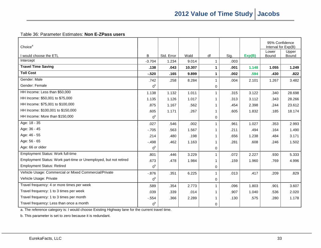
2012 Value of Time Study Jacobs
EurekaFacts, LLC 33
Table 36: Parameter Estimates: Non E-ZPass users
Choicea
B Std. Error Wald df Sig. Exp(B)
95% Confidence Interval for Exp(B)
I would choose the ETL Lower Bound
Upper Bound
Intercept -3.704 1.234 9.014 1 .003
Travel Time Saving .138 .043 10.307 1 .001 1.148 1.055 1.249
Toll Cost -.520 .165 9.899 1 .002 .594 .430 .822
Gender: Male .742 .258 8.284 1 .004 2.101 1.267 3.482
Gender: Female 0b 0
HH Income: Less than $50,000 1.138 1.132 1.011 1 .315 3.122 .340 28.698
HH Income: $50,001 to $75,000 1.135 1.126 1.017 1 .313 3.112 .343 28.266
HH Income: $75,001 to $100,000 .875 1.167 .562 1 .454 2.398 .244 23.612
HH Income: $100,001 to $150,000 .605 1.171 .267 1 .605 1.832 .185 18.174
HH Income: More than $150,000 0b 0
Age: 18 - 35 .027 .546 .002 1 .961 1.027 .353 2.993
Age: 36 - 45 -.705 .563 1.567 1 .211 .494 .164 1.490
Age: 46 - 55 .214 .480 .198 1 .656 1.238 .484 3.171
Age: 56 - 65 -.498 .462 1.163 1 .281 .608 .246 1.502
Age: 66 or older 0b 0
Employment Status: Work full-time .801 .446 3.229 1 .072 2.227 .930 5.333
Employment Status: Work part-time or Unemployed, but not retired .673 .478 1.984 1 .159 1.960 .769 4.996
Employment Status: Retired 0b 0
Vehicle Usage: Commercial or Mixed Commercial/Private -.876 .351 6.225 1 .013 .417 .209 .829
Vehicle Usage: Private 0b 0
Travel frequency: 4 or more times per week .589 .354 2.773 1 .096 1.803 .901 3.607
Travel frequency: 1 to 3 times per week .039 .339 .014 1 .907 1.040 .536 2.020
Travel frequency: 1 to 3 times per month -.554 .366 2.289 1 .130 .575 .280 1.178
Travel frequency: Less than once a month 0b 0
a. The reference category is: I would choose Existing Highway lane for the current travel time.
b. This parameter is set to zero because it is redundant.
2012 Value of Time Study Jacobs
EurekaFacts, LLC 34
QUESTIONNAIRE

2012 Value of Time Study Jacobs
EurekaFacts, LLC 35
Maryland Transportation Authority Survey
Welcome to the Maryland Transportation Authority Survey!
EurekaFacts is conducting this survey on behalf of MDTA, to assess motorists’ needs and travel preferences.
Part A- About your recent travel
1. Do you currently have a valid driver’s license?
• Yes • No (Terminate)
We would first like to ask you some questions about your recent vehicle trips.
2. How often, if at all, do you travel on the I-95 Highway section between the I-95/I-895 merge and MD 43/White Marsh Boulevard in either direction? Please see the map below. The I-95 Highway section in question is marked on the map between the two red locations.
4 or more times per week (Skip to Q. 4) 2 to 3 times per week (Skip to Q. 4) Once a week (Skip to Q. 4) 1 to 3 times per month (Skip to Q. 4) Less than once a month, but more than twice a year (Skip to Q. 4) 2 times per year or less (Go to Q.3 and then Q. 4, do not skip to Part D) Never (Go to Q.3)
[INSERT MAP]
3. What is the reason that you are not using, or rarely using, the I-95 Highway section between the I- 95/I-895 merge and MD 43/White Marsh Boulevard?
Not on my way to where I need to go (If answered “Never” in Q2, Terminate) Traffic congestion (If answered “Never” in Q2, skip to Part D) Other (Please specify) (If answered “Never” in Q2, skip to Part D)
Please think of the most recent trip in which you passed through the I-95 Highway section between the I-95/I-895 merge and MD/43 White Marsh Boulevard. For all of the following questions, please answer based on this specific trip.
____________________________________________________________________________________
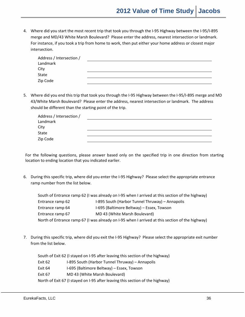
2012 Value of Time Study Jacobs
EurekaFacts, LLC 36
4. Where did you start the most recent trip that took you through the I-95 Highway between the I-95/I-895 merge and MD/43 White Marsh Boulevard? Please enter the address, nearest intersection or landmark. For instance, if you took a trip from home to work, then put either your home address or closest major intersection.
Address / Intersection / Landmark
City State Zip Code
5. Where did you end this trip that took you through the I-95 Highway between the I-95/I-895 merge and MD
43/White Marsh Boulevard? Please enter the address, nearest intersection or landmark. The address should be different than the starting point of the trip.
Address / Intersection / Landmark
City State Zip Code
For the following questions, please answer based only on the specified trip in one direction from starting location to ending location that you indicated earlier.
6. During this specific trip, where did you enter the I-95 Highway? Please select the appropriate entrance ramp number from the list below.
South of Entrance ramp 62 (I was already on I-95 when I arrived at this section of the highway) Entrance ramp 62 I-895 South (Harbor Tunnel Thruway) – Annapolis Entrance ramp 64 I-695 (Baltimore Beltway) – Essex, Towson Entrance ramp 67 MD 43 (White Marsh Boulevard) North of Entrance ramp 67 (I was already on I-95 when I arrived at this section of the highway)
7. During this specific trip, where did you exit the I-95 Highway? Please select the appropriate exit number from the list below.
South of Exit 62 (I stayed on I-95 after leaving this section of the highway) Exit 62 I-895 South (Harbor Tunnel Thruway) – Annapolis Exit 64 I-695 (Baltimore Beltway) – Essex, Towson Exit 67 MD 43 (White Marsh Boulevard) North of Exit 67 (I stayed on I-95 after leaving this section of the highway)
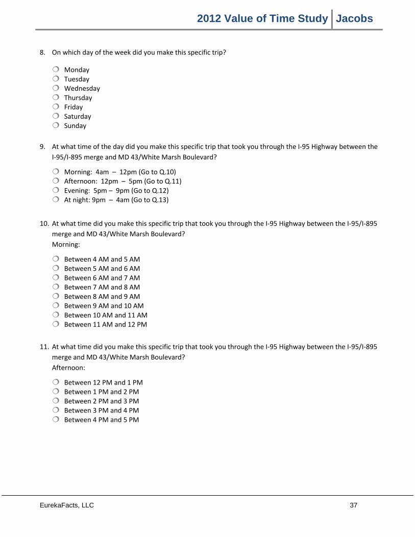
2012 Value of Time Study Jacobs
EurekaFacts, LLC 37
8. On which day of the week did you make this specific trip?
Monday Tuesday Wednesday Thursday Friday Saturday Sunday
9. At what time of the day did you make this specific trip that took you through the I-95 Highway between the I-95/I-895 merge and MD 43/White Marsh Boulevard?
Morning: 4am – 12pm (Go to Q.10) Afternoon: 12pm – 5pm (Go to Q.11) Evening: 5pm – 9pm (Go to Q.12) At night: 9pm – 4am (Go to Q.13)
10. At what time did you make this specific trip that took you through the I-95 Highway between the I-95/I-895
merge and MD 43/White Marsh Boulevard? Morning:
Between 4 AM and 5 AM Between 5 AM and 6 AM Between 6 AM and 7 AM Between 7 AM and 8 AM Between 8 AM and 9 AM Between 9 AM and 10 AM Between 10 AM and 11 AM Between 11 AM and 12 PM
11. At what time did you make this specific trip that took you through the I-95 Highway between the I-95/I-895 merge and MD 43/White Marsh Boulevard? Afternoon:
Between 12 PM and 1 PM Between 1 PM and 2 PM Between 2 PM and 3 PM Between 3 PM and 4 PM Between 4 PM and 5 PM

2012 Value of Time Study Jacobs
EurekaFacts, LLC 38
12. At what time did you make this specific trip that took you through the I-95 Highway between the I-95/I-895 merge and MD 43/White Marsh Boulevard? Evening:
Between 5 PM and 6 PM Between 6 PM and 7 PM Between 7 PM and 8 PM Between 8 PM and 9 PM
13. At what time did you make this specific trip that took you through the I-95 Highway between the I-95/I-895
merge and MD 43/White Marsh Boulevard? At night:
Between 9 PM and 10 PM Between 10 PM and 11 PM Between 11 PM and 12 AM Between 12 AM and 1 AM Between 1 AM and 2 AM Between 2 AM and 3 AM Between 3 AM and 4 AM
14. What was your primary purpose for this specific trip that took you through the I-95 Highway between the I-95/I-895 merge and White Marsh Boulevard?
Commuting to / from work Work-related travel To / from school Shopping / Errands / Personal Appointment Social / Dining / Entertainment Recreation / Sports Other (Please specify)
15. How often do you make this particular trip for the specified trip purpose, in this one direction (from starting location that you noted to ending location that you noted) via the same route?
4 or more times per week 2 to 3 times per week 1 time per week 1 to 3 times per month Less than 1 time per month but more than 2 times per year 2 times per year or less (Skip to Q. 17)
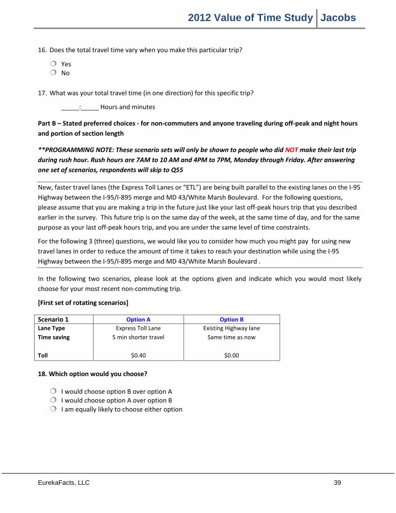
2012 Value of Time Study Jacobs
EurekaFacts, LLC 39
16. Does the total travel time vary when you make this particular trip?
Yes No
17. What was your total travel time (in one direction) for this specific trip?
_____:_____ Hours and minutes
Part B – Stated preferred choices - for non-commuters and anyone traveling during off-peak and night hours and portion of section length
**PROGRAMMING NOTE: These scenario sets will only be shown to people who did NOT make their last trip during rush hour. Rush hours are 7AM to 10 AM and 4PM to 7PM, Monday through Friday. After answering one set of scenarios, respondents will skip to Q55
New, faster travel lanes (the Express Toll Lanes or “ETL”) are being built parallel to the existing lanes on the I-95 Highway between the I-95/I-895 merge and MD 43/White Marsh Boulevard. For the following questions, please assume that you are making a trip in the future just like your last off-peak hours trip that you described earlier in the survey. This future trip is on the same day of the week, at the same time of day, and for the same purpose as your last off-peak hours trip, and you are under the same level of time constraints.
For the following 3 (three) questions, we would like you to consider how much you might pay for using new travel lanes in order to reduce the amount of time it takes to reach your destination while using the I-95 Highway between the I-95/I-895 merge and MD 43/White Marsh Boulevard .
In the following two scenarios, please look at the options given and indicate which you would most likely choose for your most recent non-commuting trip.
[First set of rotating scenarios]
Scenario 1 Option A Option B Lane Type Time saving Toll
Express Toll Lane 5 min shorter travel
$0.40
Existing Highway lane Same time as now
$0.00
18. Which option would you choose?
I would choose option B over option A I would choose option A over option B I am equally likely to choose either option
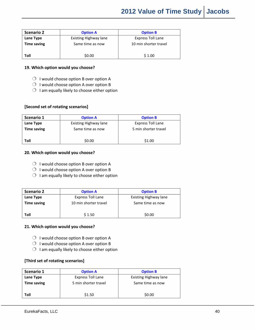
2012 Value of Time Study Jacobs
EurekaFacts, LLC 40
Scenario 2 Option A Option B Lane Type Time saving Toll
Existing Highway lane Same time as now
$0.00
Express Toll Lane 10 min shorter travel
$ 1.00
19. Which option would you choose?
I would choose option B over option A I would choose option A over option B I am equally likely to choose either option
[Second set of rotating scenarios]
Scenario 1 Option A Option B Lane Type Time saving Toll
Existing Highway lane Same time as now
$0.00
Express Toll Lane 5 min shorter travel
$1.00
20. Which option would you choose?
I would choose option B over option A I would choose option A over option B I am equally likely to choose either option
Scenario 2 Option A Option B Lane Type Time saving Toll
Express Toll Lane 10 min shorter travel
$ 1.50
Existing Highway lane Same time as now
$0.00
21. Which option would you choose?
I would choose option B over option A I would choose option A over option B I am equally likely to choose either option
[Third set of rotating scenarios]
Scenario 1 Option A Option B Lane Type Time saving Toll
Express Toll Lane 5 min shorter travel
$1.50
Existing Highway lane Same time as now
$0.00
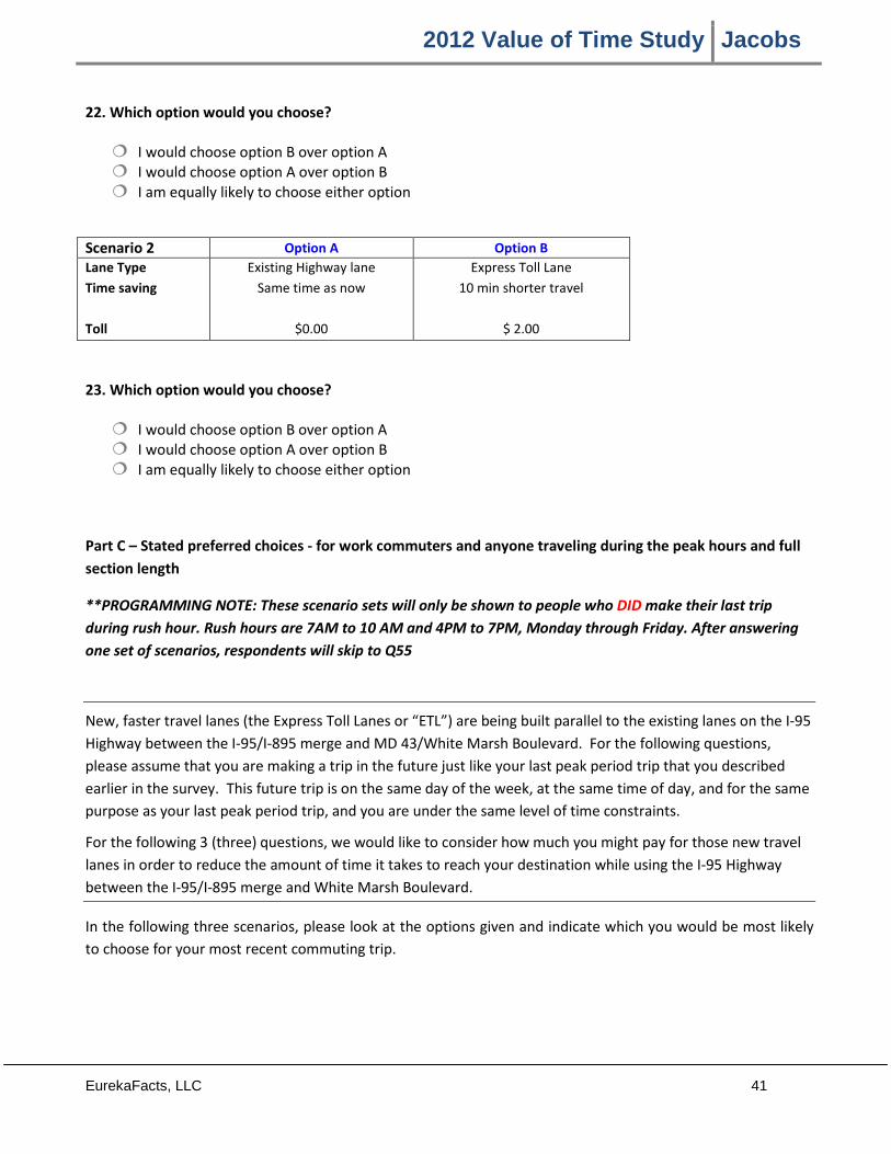
2012 Value of Time Study Jacobs
EurekaFacts, LLC 41
22. Which option would you choose?
I would choose option B over option A I would choose option A over option B I am equally likely to choose either option
Scenario 2 Option A Option B Lane Type Time saving Toll
Existing Highway lane Same time as now
$0.00
Express Toll Lane 10 min shorter travel
$ 2.00
23. Which option would you choose?
I would choose option B over option A I would choose option A over option B I am equally likely to choose either option
Part C – Stated preferred choices - for work commuters and anyone traveling during the peak hours and full section length
**PROGRAMMING NOTE: These scenario sets will only be shown to people who DID make their last trip during rush hour. Rush hours are 7AM to 10 AM and 4PM to 7PM, Monday through Friday. After answering one set of scenarios, respondents will skip to Q55
New, faster travel lanes (the Express Toll Lanes or “ETL”) are being built parallel to the existing lanes on the I-95 Highway between the I-95/I-895 merge and MD 43/White Marsh Boulevard. For the following questions, please assume that you are making a trip in the future just like your last peak period trip that you described earlier in the survey. This future trip is on the same day of the week, at the same time of day, and for the same purpose as your last peak period trip, and you are under the same level of time constraints.
For the following 3 (three) questions, we would like to consider how much you might pay for those new travel lanes in order to reduce the amount of time it takes to reach your destination while using the I-95 Highway between the I-95/I-895 merge and White Marsh Boulevard.
In the following three scenarios, please look at the options given and indicate which you would be most likely to choose for your most recent commuting trip.
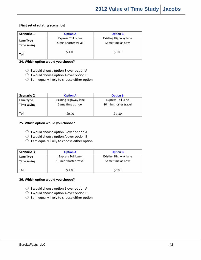
2012 Value of Time Study Jacobs
EurekaFacts, LLC 42
[First set of rotating scenarios]
Scenario 1 Option A Option B
Lane Type Time saving Toll
Express Toll Lanes 5 min shorter travel
$ 1.00
Existing Highway lane Same time as now
$0.00
24. Which option would you choose?
I would choose option B over option A I would choose option A over option B I am equally likely to choose either option
Scenario 2 Option A Option B Lane Type Time saving Toll
Existing Highway lane Same time as now
$0.00
Express Toll Lane 10 min shorter travel
$ 1.50
25. Which option would you choose?
I would choose option B over option A I would choose option A over option B I am equally likely to choose either option
Scenario 3 Option A Option B Lane Type Time saving Toll
Express Toll Lane 15 min shorter travel
$ 2.00
Existing Highway lane Same time as now
$0.00
26. Which option would you choose?
I would choose option B over option A I would choose option A over option B I am equally likely to choose either option
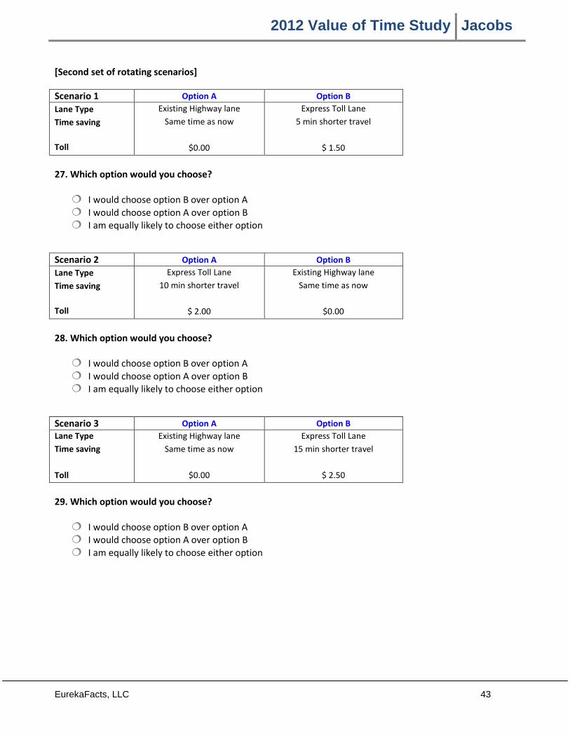
2012 Value of Time Study Jacobs
EurekaFacts, LLC 43
[Second set of rotating scenarios]
Scenario 1 Option A Option B Lane Type Time saving Toll
Existing Highway lane Same time as now
$0.00
Express Toll Lane 5 min shorter travel
$ 1.50
27. Which option would you choose?
I would choose option B over option A I would choose option A over option B I am equally likely to choose either option
Scenario 2 Option A Option B Lane Type Time saving Toll
Express Toll Lane 10 min shorter travel
$ 2.00
Existing Highway lane Same time as now
$0.00
28. Which option would you choose?
I would choose option B over option A I would choose option A over option B I am equally likely to choose either option
Scenario 3 Option A Option B Lane Type Time saving Toll
Existing Highway lane Same time as now
$0.00
Express Toll Lane 15 min shorter travel
$ 2.50
29. Which option would you choose?
I would choose option B over option A I would choose option A over option B I am equally likely to choose either option
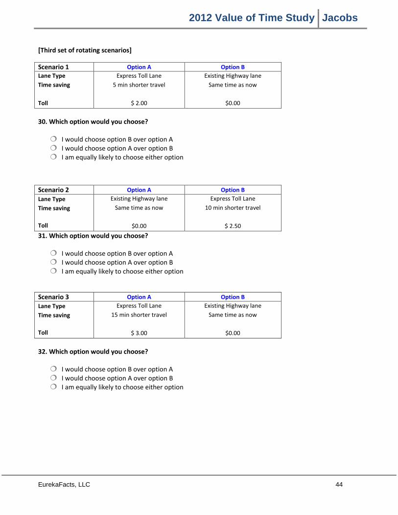
2012 Value of Time Study Jacobs
EurekaFacts, LLC 44
[Third set of rotating scenarios]
Scenario 1 Option A Option B Lane Type Time saving Toll
Express Toll Lane 5 min shorter travel
$ 2.00
Existing Highway lane Same time as now
$0.00
30. Which option would you choose?
I would choose option B over option A I would choose option A over option B I am equally likely to choose either option
Scenario 2 Option A Option B Lane Type Time saving Toll
Existing Highway lane Same time as now
$0.00
Express Toll Lane 10 min shorter travel
$ 2.50
31. Which option would you choose?
I would choose option B over option A I would choose option A over option B I am equally likely to choose either option
Scenario 3 Option A Option B Lane Type Time saving Toll
Express Toll Lane 15 min shorter travel
$ 3.00
Existing Highway lane Same time as now
$0.00
32. Which option would you choose?
I would choose option B over option A I would choose option A over option B I am equally likely to choose either option
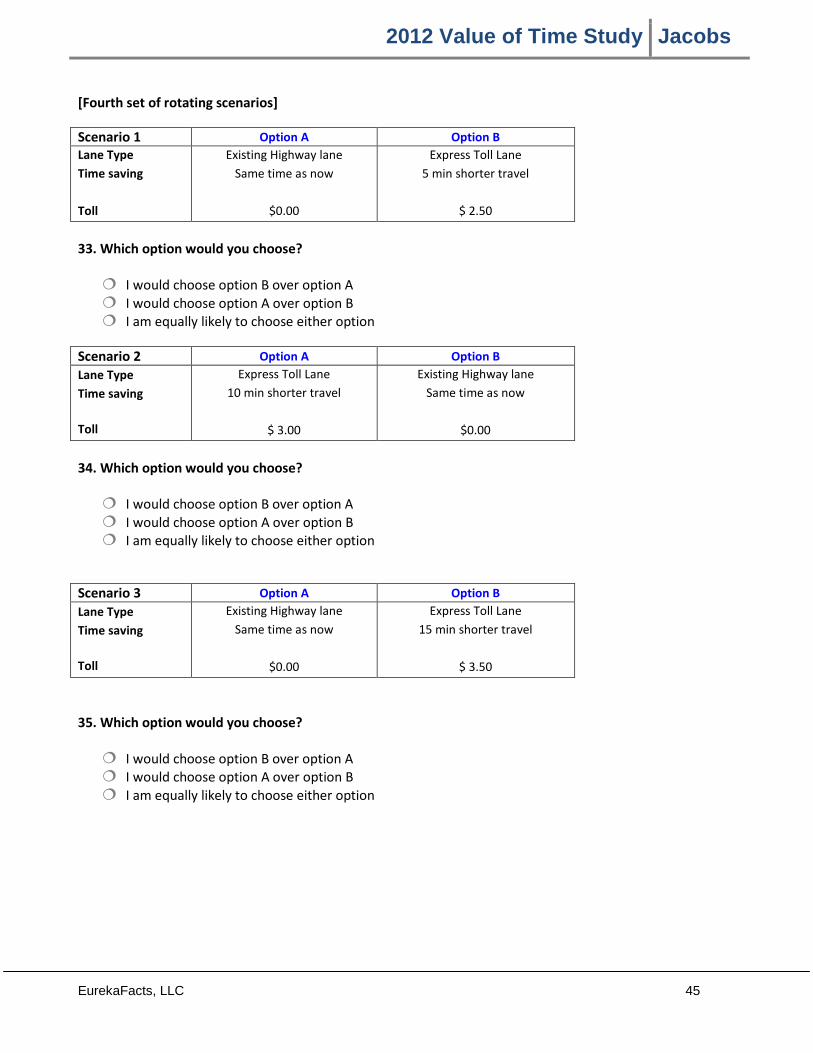
2012 Value of Time Study Jacobs
EurekaFacts, LLC 45
[Fourth set of rotating scenarios]
Scenario 1 Option A Option B Lane Type Time saving Toll
Existing Highway lane Same time as now
$0.00
Express Toll Lane 5 min shorter travel
$ 2.50
33. Which option would you choose?
I would choose option B over option A I would choose option A over option B I am equally likely to choose either option
Scenario 2 Option A Option B Lane Type Time saving Toll
Express Toll Lane 10 min shorter travel
$ 3.00
Existing Highway lane Same time as now
$0.00
34. Which option would you choose?
I would choose option B over option A I would choose option A over option B I am equally likely to choose either option
Scenario 3 Option A Option B Lane Type Time saving Toll
Existing Highway lane Same time as now
$0.00
Express Toll Lane 15 min shorter travel
$ 3.50
35. Which option would you choose?
I would choose option B over option A I would choose option A over option B I am equally likely to choose either option
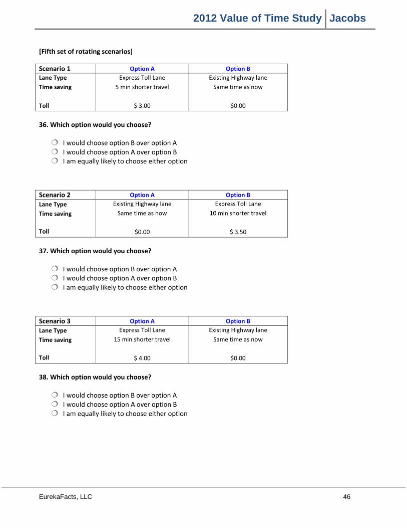
2012 Value of Time Study Jacobs
EurekaFacts, LLC 46
[Fifth set of rotating scenarios]
Scenario 1 Option A Option B Lane Type Time saving Toll
Express Toll Lane 5 min shorter travel
$ 3.00
Existing Highway lane Same time as now
$0.00
36. Which option would you choose?
I would choose option B over option A I would choose option A over option B I am equally likely to choose either option
Scenario 2 Option A Option B Lane Type Time saving Toll
Existing Highway lane Same time as now
$0.00
Express Toll Lane 10 min shorter travel
$ 3.50
37. Which option would you choose?
I would choose option B over option A I would choose option A over option B I am equally likely to choose either option
Scenario 3 Option A Option B Lane Type Time saving Toll
Express Toll Lane 15 min shorter travel
$ 4.00
Existing Highway lane Same time as now
$0.00
38. Which option would you choose?
I would choose option B over option A I would choose option A over option B I am equally likely to choose either option
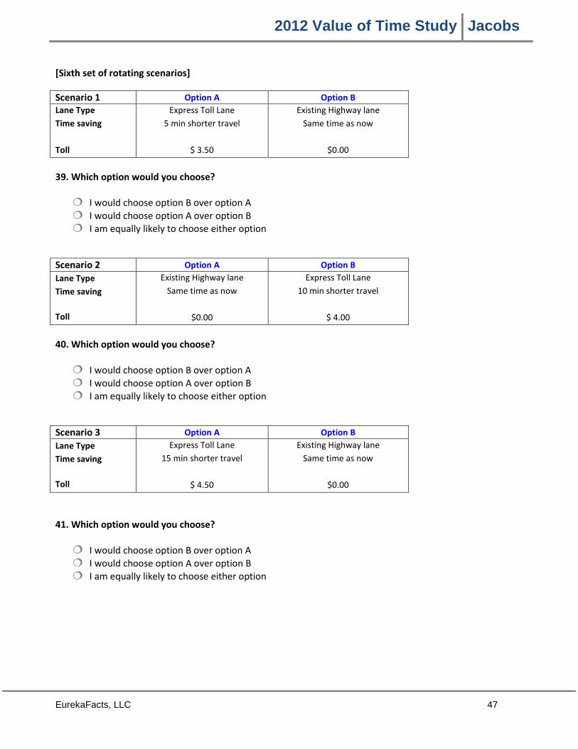
2012 Value of Time Study Jacobs
EurekaFacts, LLC 47
[Sixth set of rotating scenarios]
Scenario 1 Option A Option B Lane Type Time saving Toll
Express Toll Lane 5 min shorter travel
$ 3.50
Existing Highway lane Same time as now
$0.00
39. Which option would you choose?
I would choose option B over option A I would choose option A over option B I am equally likely to choose either option
Scenario 2 Option A Option B Lane Type Time saving Toll
Existing Highway lane Same time as now
$0.00
Express Toll Lane 10 min shorter travel
$ 4.00
40. Which option would you choose?
I would choose option B over option A I would choose option A over option B I am equally likely to choose either option
Scenario 3 Option A Option B Lane Type Time saving Toll
Express Toll Lane 15 min shorter travel
$ 4.50
Existing Highway lane Same time as now
$0.00
41. Which option would you choose?
I would choose option B over option A I would choose option A over option B I am equally likely to choose either option

2012 Value of Time Study Jacobs
EurekaFacts, LLC 48
[Seventh set of rotating scenarios]
Scenario 1 Option A Option B Lane Type Time saving Toll
Existing Highway lane Same time as now
$0.00
Express Toll Lane 5 min shorter travel
$ 4.00
42. Which option would you choose?
I would choose option B over option A I would choose option A over option B I am equally likely to choose either option
Scenario 2 Option A Option B Lane Type Time saving Toll
Express Toll Lane 10 min shorter travel
$ 4.50
Existing Highway lane Same time as now
$0.00
43. Which option would you choose?
I would choose option B over option A I would choose option A over option B I am equally likely to choose either option
Scenario 3 Option A Option B Lane Type Time saving Toll
Existing Highway lane Same time as now
$0.00
Express Toll Lane 15 min shorter travel
$ 5.00
44. Which option would you choose?
I would choose option B over option A I would choose option A over option B I am equally likely to choose either option
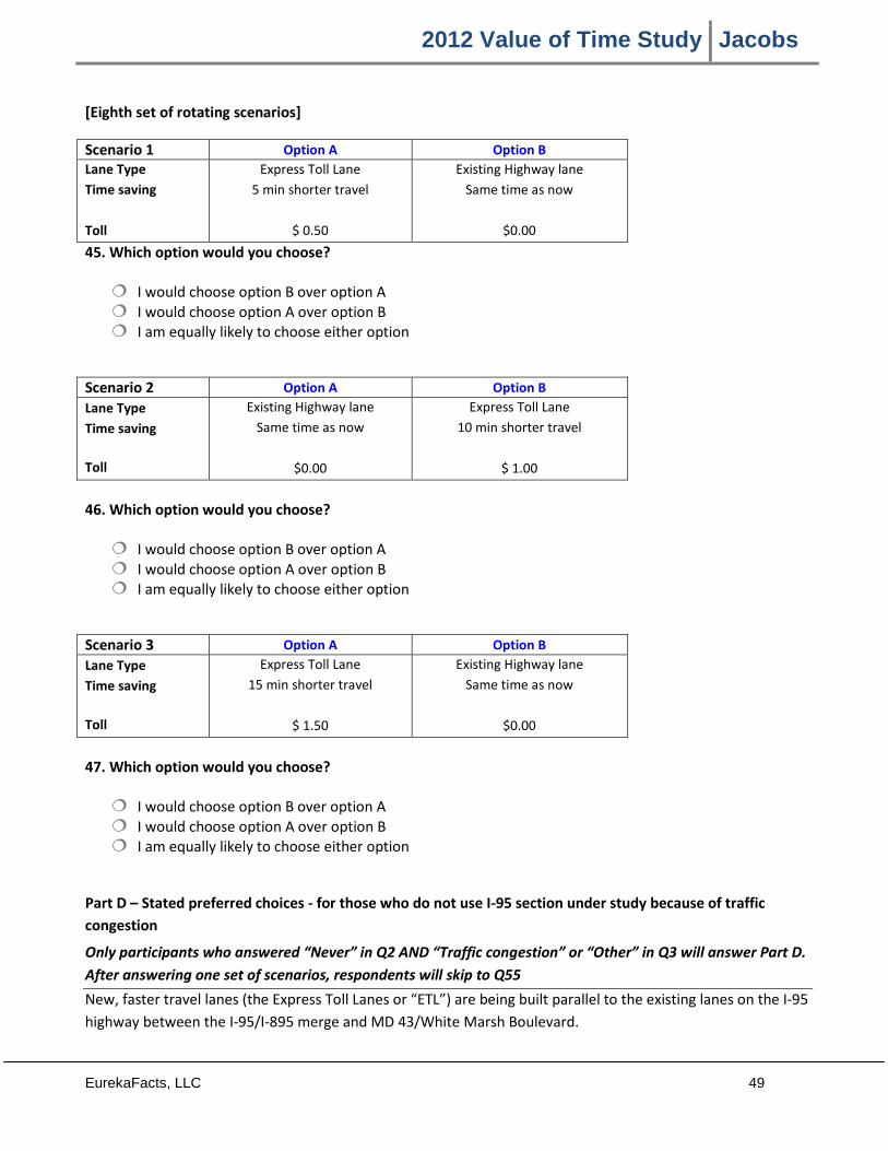
2012 Value of Time Study Jacobs
EurekaFacts, LLC 49
[Eighth set of rotating scenarios]
Scenario 1 Option A Option B Lane Type Time saving Toll
Express Toll Lane 5 min shorter travel
$ 0.50
Existing Highway lane Same time as now
$0.00
45. Which option would you choose?
I would choose option B over option A I would choose option A over option B I am equally likely to choose either option
Scenario 2 Option A Option B Lane Type Time saving Toll
Existing Highway lane Same time as now
$0.00
Express Toll Lane 10 min shorter travel
$ 1.00
46. Which option would you choose?
I would choose option B over option A I would choose option A over option B I am equally likely to choose either option
Scenario 3 Option A Option B Lane Type Time saving Toll
Express Toll Lane 15 min shorter travel
$ 1.50
Existing Highway lane Same time as now
$0.00
47. Which option would you choose?
I would choose option B over option A I would choose option A over option B I am equally likely to choose either option
Part D – Stated preferred choices - for those who do not use I-95 section under study because of traffic congestion
Only participants who answered “Never” in Q2 AND “Traffic congestion” or “Other” in Q3 will answer Part D. After answering one set of scenarios, respondents will skip to Q55 New, faster travel lanes (the Express Toll Lanes or “ETL”) are being built parallel to the existing lanes on the I-95 highway between the I-95/I-895 merge and MD 43/White Marsh Boulevard.
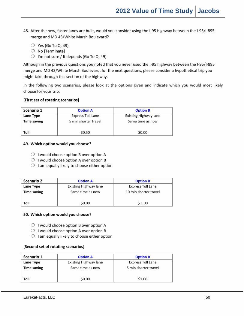
2012 Value of Time Study Jacobs
EurekaFacts, LLC 50
48. After the new, faster lanes are built, would you consider using the I-95 highway between the I-95/I-895 merge and MD 43/White Marsh Boulevard?
Yes (Go To Q. 49) No [Terminate] I'm not sure / It depends (Go To Q. 49)
Although in the previous questions you noted that you never used the I-95 highway between the I-95/I-895 merge and MD 43/White Marsh Boulevard, for the next questions, please consider a hypothetical trip you might take through this section of the highway.
In the following two scenarios, please look at the options given and indicate which you would most likely choose for your trip.
[First set of rotating scenarios]
Scenario 1 Option A Option B Lane Type Time saving Toll
Express Toll Lane 5 min shorter travel
$0.50
Existing Highway lane Same time as now
$0.00
49. Which option would you choose?
I would choose option B over option A I would choose option A over option B I am equally likely to choose either option
Scenario 2 Option A Option B Lane Type Time saving Toll
Existing Highway lane Same time as now
$0.00
Express Toll Lane 10 min shorter travel
$ 1.00
50. Which option would you choose?
I would choose option B over option A I would choose option A over option B I am equally likely to choose either option
[Second set of rotating scenarios]
Scenario 1 Option A Option B Lane Type Time saving Toll
Existing Highway lane Same time as now
$0.00
Express Toll Lane 5 min shorter travel
$1.00
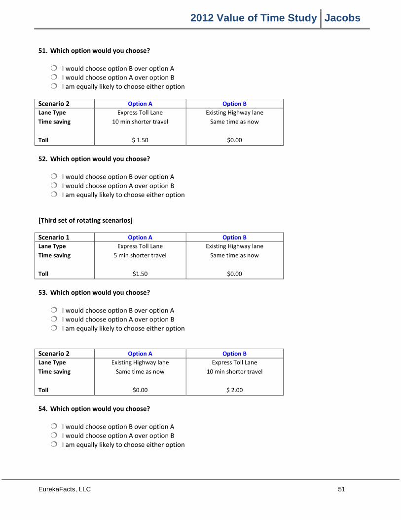
2012 Value of Time Study Jacobs
EurekaFacts, LLC 51
51. Which option would you choose?
I would choose option B over option A I would choose option A over option B I am equally likely to choose either option
Scenario 2 Option A Option B Lane Type Time saving Toll
Express Toll Lane 10 min shorter travel
$ 1.50
Existing Highway lane Same time as now
$0.00
52. Which option would you choose?
I would choose option B over option A I would choose option A over option B I am equally likely to choose either option
[Third set of rotating scenarios]
Scenario 1 Option A Option B Lane Type Time saving Toll
Express Toll Lane 5 min shorter travel
$1.50
Existing Highway lane Same time as now
$0.00
53. Which option would you choose?
I would choose option B over option A I would choose option A over option B I am equally likely to choose either option
Scenario 2 Option A Option B Lane Type Time saving Toll
Existing Highway lane Same time as now
$0.00
Express Toll Lane 10 min shorter travel
$ 2.00
54. Which option would you choose?
I would choose option B over option A I would choose option A over option B I am equally likely to choose either option

2012 Value of Time Study Jacobs
EurekaFacts, LLC 52
55. Rate the following factors in terms of importance when choosing your driving route for any commuting or other job-related purpose:
Extremely Important
Very Important Somewhat Important
Not Very Important
Not Important
Time savings
Avoiding traffic congestion
Low cost
Trip safety
56. What type of vehicle do you drive most often? (Select one)
Passenger car, SUV, or pick-up truck (2-axle private vehicle) Motorcycle 2-axle truck 3-axle vehicle (including cars pulling a one axle trailer) 4-axle vehicle (including cars pulling a two axle trailer) 5-axle vehicle (including cars pulling a three axle trailer) 6-axle truck or larger Other (please specify)
57. The usage of this vehicle is:
Commercial Private Mixed (private and commercial)
58. Please mark the appropriate selection(s):
I have an E-ZPass (Skip to Q. 60) I do not have an E-ZPass, but I would obtain one if it made travel easier (Skip to Q. 60) I do not have an E-ZPass and I will not get one (Go to Q. 59)
59. What is the reason that you do not have or do not want to use the E-ZPass? (Select all that apply)
I am concerned about privacy I think it is too costly to use I have no credit card I do not use toll roads often enough I do not know what E-ZPass is Other, please specify

2012 Value of Time Study Jacobs
EurekaFacts, LLC 53
The following set of questions are asked only to ensure that this study represents the feedback and opinions from all relevant groups of drivers residing in the area and who may be interested in the I-95 ETLs under development.
60. What is your gender?
Male Female Prefer not to answer
61. Please indicate your household income range.
Less than $25,000 $25,001 to $50,000 $50,001 to $75,000 $75,001 to $100,000 $100,001 to $150,000 More than $150,000 Prefer not to answer
62. Please indicate your age
18 - 25 26 - 35 36 - 45 46 - 55 56 - 65 66 + Prefer not to answer
63. What is your employment status?
Work full-time Work part-time Temporary unemployed Do not work, but not retired Retired Prefer not to answer
Thank you for taking our survey!

APPENDIX B
Travel Demand Modeling and Microsimulation Modeling Technical Memorandum
1
81 Mosher Street Baltimore, MD 21217 Phone 410.728.2900 Fax 410.383.3270
Date: December 14, 2013
To: Joe Sobleski, Jacobs
From: James A. Burnett, P.E., PTOE, RK&K Zichuan Li, Ph.D., RK&K Robert R. Josef, RK&K
CC: Phil Eshelman, Jacobs Rick Gobeille, Jacobs Karen B. Kahl, P.E., PTOE, RK&K
Subject: I-95 Section 100 Express Toll Lanes (ETL) Study
Summary of Forecasting and Analysis Methodology and Results
The purpose of this memorandum is to document the methodology and results of RK&K’s efforts assisting Jacobs in the development of traffic volume estimates and subsequently analyzing traffic operations along I-95 and surrounding roadways after the I-95 Section 100 Express Toll Lanes (ETLs) open in Baltimore, Maryland. This work was performed for the Maryland Transportation Authority (MdTA) to help the Authority determine the appropriate toll rates to implement when the lanes open (anticipated opening in 2014), as well as in planning year 2025. In general terms, using the regional travel forecasting model, RK&K extracted volume data that was then provided to Jacobs who post-processed the raw volumes using a proprietary toll revenue model. Jacobs subsequently provided those refined volume estimates back to RK&K who used them in a VISSIM model to study the traffic operations in the ETLs and GP lanes.
Background
The I-95 Section 100 ETL study covers the roadway section from the I-95/MD 43 interchange in Baltimore County to the split of I-895 and I-95 just inside the Baltimore City limits. The northern end of the ETLs on I-95 southbound starts approximately one (1) mile north of the MD 43 interchange, and can also be accessed via a signalized ramp from both eastbound and westbound MD 43. Further south along I-95 (beyond the I-695 interchange), the southbound ETLs split into an I-895 branch and an I-95 branch. Traffic on the I-895 branch southbound ETLs can merge back onto the I-895 general purpose (GP) lanes about 2,300 feet prior to Moravia Road, or continue onto Moravia Road via a ramp in the median that terminates at a signalized intersection. The I-95 branch simply merges back onto the I-95 southbound GP lanes about 2,300 feet prior to the US 40 (Pulaski Highway) interchange.

I-95/I-895 Section 100 Express Toll Lanes Study December 14, 2013 Maryland Transportation Authority RK&K Engineers, LLP
2
Similarly, in the northbound direction, the ETLs start at the southern project limits from an I-95 branch and an I-895 branch. The northbound I-95 branch starts just north of the US 40 (Pulaski Highway) interchange. The northbound I-895 branch starts at the Moravia Road interchange, where traffic from the Moravia Road overpass can enter the ETLs via a signalized ramp in the median of I-895. Traffic from the northbound I-895 GP lanes can also enter the ETLs approximately 1,700 feet north of the Moravia Road interchange. The northbound I-895 ETLs branch merges with the northbound I-95 ETLs branch and continues beyond I-695 to the MD 43 interchange. Northbound ETL traffic can exit the ETLs to both eastbound and westbound MD 43 via a signalized ramp in the I-95 median, or they can merge back into northbound I-95 GP lanes approximately one (1) mile north of the MD 43 interchange. The following intersections and interchanges were included in this study (from north to south):
1. MD 43 (White Marsh Boulevard) at Honeygo Boulevard intersection 2. I-95 at MD 43 interchange including ETLs to/from I-95 3. MD 43 at MD 7 (Philadelphia Road) interchangeI-695 at US 1 (Belair Road) interchange 4. I-95 at I-695 interchange without ETL access ramps 5. I-695 at MD 7 (Philadelphia Road) interchange 6. I-95 at I-895 split, including ETL split to I-95 and I-895 7. I-895 at Moravia Road interchange, including ETL ramps to/from I-95) 8. I-95 at US 40 (Pulaski Highway) interchange with ETL access ramp
The two major components of RK&K’s study were traffic volume estimates and VISSIM simulation analysis, and the details of those efforts are summarized in the following sections.
Traffic Volume Estimates
RK&K prepared traffic volume estimates within the study limits for the following scenarios:
Existing 2012
ETLs opening year 2015 (approximately corresponding to the actual anticipated ETL opening year of 2014, but using 2015 for simplicity to correspond with the regional transportation model);
Long-range planning year 2025
Existing Traffic Counts and Origin-Destination Matrix
RK&K received VISSIM simulation models from MdTA which were developed by Parsons Brinckerhoff & URS Corporation, with documentation dated March 20, 2012. Those VISSIM models represented a 2014 opening year scenario for the I-95 ETLs. To validate the volumes that were included in those models, RK&K performed a comparison of the traffic volumes from the VISSIM models and actual traffic counts along I-895 and I-95 to south of the I-95/I-895 split (see Figure 1 for details). These counts were collected by RK&K in 2009 and 2012 under a separate contract with MdTA. The comparison results are listed in Table 1.
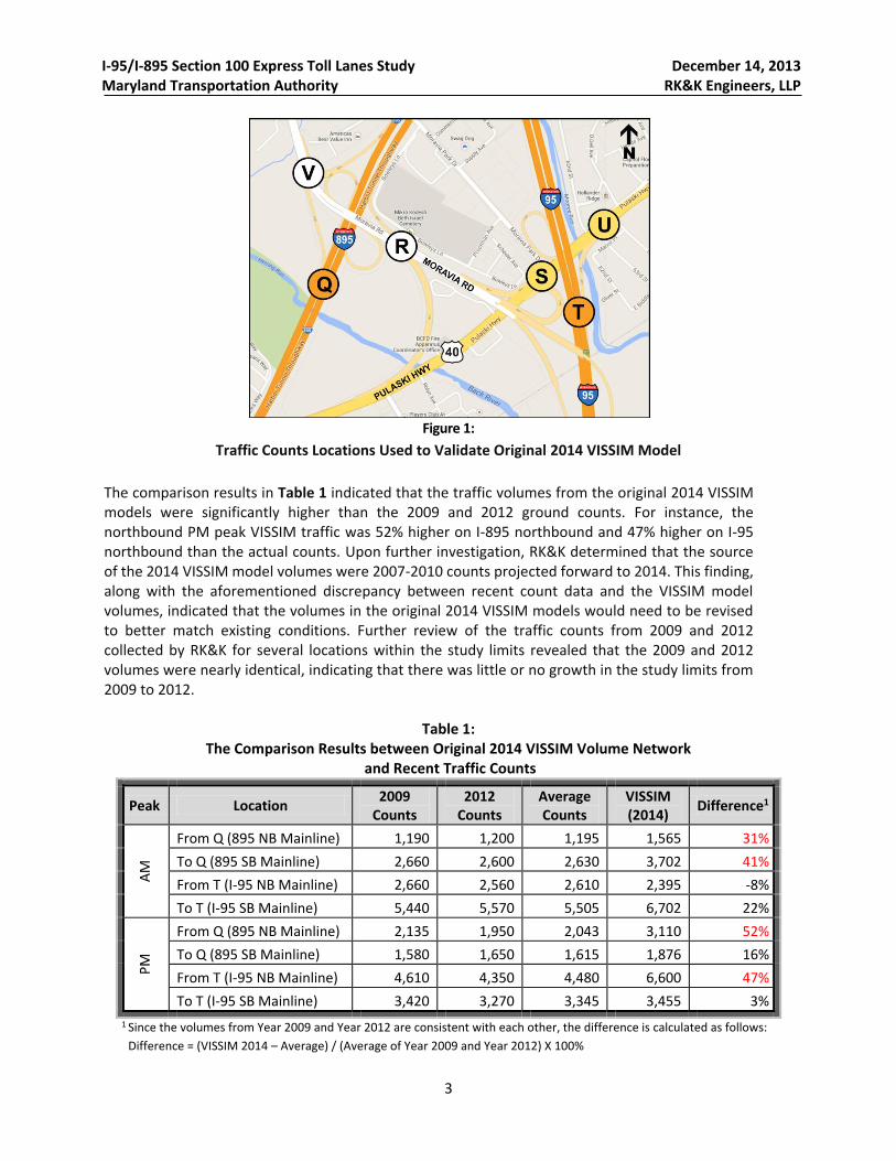
I-95/I-895 Section 100 Express Toll Lanes Study December 14, 2013 Maryland Transportation Authority RK&K Engineers, LLP
3
Figure 1:
Traffic Counts Locations Used to Validate Original 2014 VISSIM Model
The comparison results in Table 1 indicated that the traffic volumes from the original 2014 VISSIM models were significantly higher than the 2009 and 2012 ground counts. For instance, the northbound PM peak VISSIM traffic was 52% higher on I-895 northbound and 47% higher on I-95 northbound than the actual counts. Upon further investigation, RK&K determined that the source of the 2014 VISSIM model volumes were 2007-2010 counts projected forward to 2014. This finding, along with the aforementioned discrepancy between recent count data and the VISSIM model volumes, indicated that the volumes in the original 2014 VISSIM models would need to be revised to better match existing conditions. Further review of the traffic counts from 2009 and 2012 collected by RK&K for several locations within the study limits revealed that the 2009 and 2012 volumes were nearly identical, indicating that there was little or no growth in the study limits from 2009 to 2012.
Table 1: The Comparison Results between Original 2014 VISSIM Volume Network
and Recent Traffic Counts
Peak Location 2009
Counts 2012
Counts Average Counts
VISSIM (2014)
Difference1
AM
From Q (895 NB Mainline) 1,190 1,200 1,195 1,565 31%
To Q (895 SB Mainline) 2,660 2,600 2,630 3,702 41%
From T (I-95 NB Mainline) 2,660 2,560 2,610 2,395 -8%
To T (I-95 SB Mainline) 5,440 5,570 5,505 6,702 22%
PM
From Q (895 NB Mainline) 2,135 1,950 2,043 3,110 52%
To Q (895 SB Mainline) 1,580 1,650 1,615 1,876 16%
From T (I-95 NB Mainline) 4,610 4,350 4,480 6,600 47%
To T (I-95 SB Mainline) 3,420 3,270 3,345 3,455 3%
1 Since the volumes from Year 2009 and Year 2012 are consistent with each other, the difference is calculated as follows:
Difference = (VISSIM 2014 – Average) / (Average of Year 2009 and Year 2012) X 100%
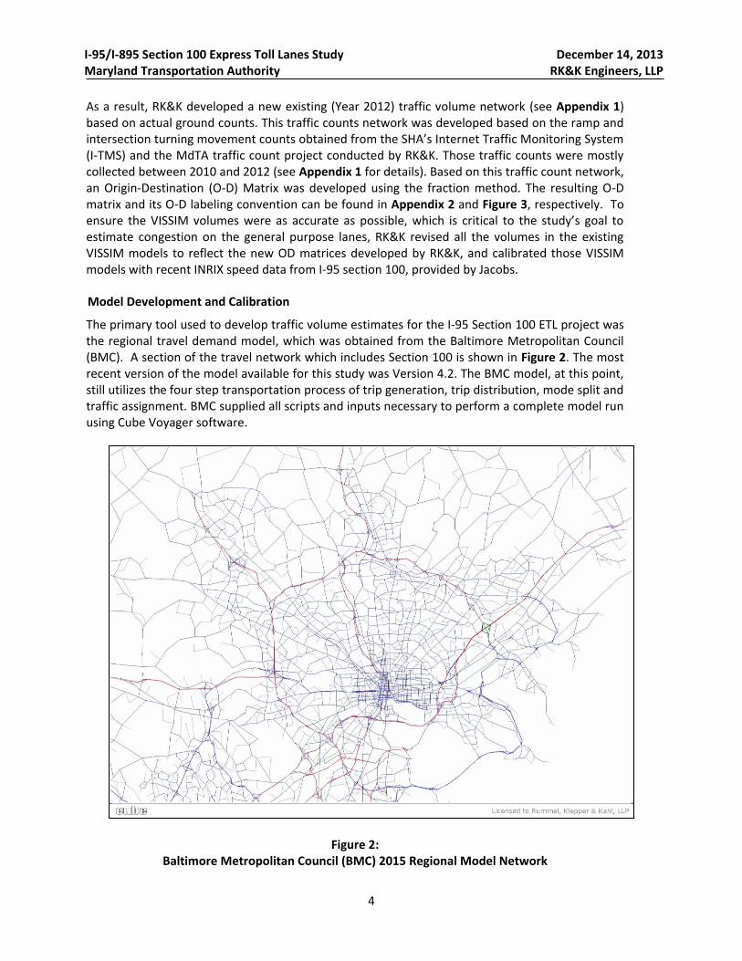
I-95/I-895 Section 100 Express Toll Lanes Study December 14, 2013 Maryland Transportation Authority RK&K Engineers, LLP
4
As a result, RK&K developed a new existing (Year 2012) traffic volume network (see Appendix 1) based on actual ground counts. This traffic counts network was developed based on the ramp and intersection turning movement counts obtained from the SHA’s Internet Traffic Monitoring System (I-TMS) and the MdTA traffic count project conducted by RK&K. Those traffic counts were mostly collected between 2010 and 2012 (see Appendix 1 for details). Based on this traffic count network, an Origin-Destination (O-D) Matrix was developed using the fraction method. The resulting O-D matrix and its O-D labeling convention can be found in Appendix 2 and Figure 3, respectively. To ensure the VISSIM volumes were as accurate as possible, which is critical to the study’s goal to estimate congestion on the general purpose lanes, RK&K revised all the volumes in the existing VISSIM models to reflect the new OD matrices developed by RK&K, and calibrated those VISSIM models with recent INRIX speed data from I-95 section 100, provided by Jacobs. Model Development and Calibration
The primary tool used to develop traffic volume estimates for the I-95 Section 100 ETL project was the regional travel demand model, which was obtained from the Baltimore Metropolitan Council (BMC). A section of the travel network which includes Section 100 is shown in Figure 2. The most recent version of the model available for this study was Version 4.2. The BMC model, at this point, still utilizes the four step transportation process of trip generation, trip distribution, mode split and traffic assignment. BMC supplied all scripts and inputs necessary to perform a complete model run using Cube Voyager software.
Figure 2:
Baltimore Metropolitan Council (BMC) 2015 Regional Model Network
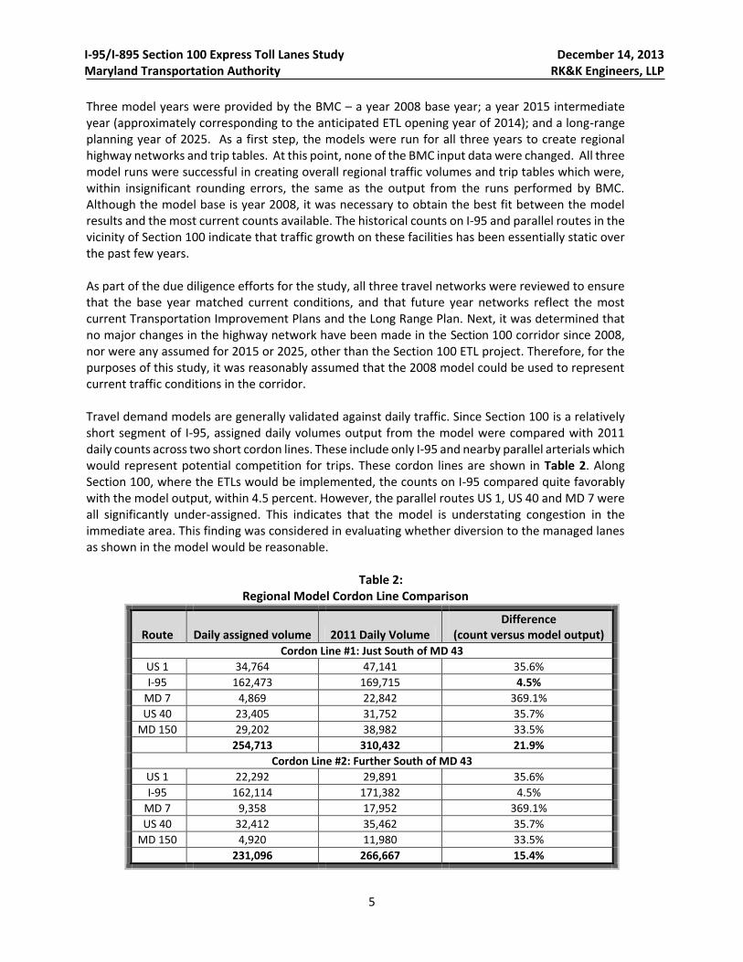
I-95/I-895 Section 100 Express Toll Lanes Study December 14, 2013 Maryland Transportation Authority RK&K Engineers, LLP
5
Three model years were provided by the BMC – a year 2008 base year; a year 2015 intermediate year (approximately corresponding to the anticipated ETL opening year of 2014); and a long-range planning year of 2025. As a first step, the models were run for all three years to create regional highway networks and trip tables. At this point, none of the BMC input data were changed. All three model runs were successful in creating overall regional traffic volumes and trip tables which were, within insignificant rounding errors, the same as the output from the runs performed by BMC. Although the model base is year 2008, it was necessary to obtain the best fit between the model results and the most current counts available. The historical counts on I-95 and parallel routes in the vicinity of Section 100 indicate that traffic growth on these facilities has been essentially static over the past few years. As part of the due diligence efforts for the study, all three travel networks were reviewed to ensure that the base year matched current conditions, and that future year networks reflect the most current Transportation Improvement Plans and the Long Range Plan. Next, it was determined that no major changes in the highway network have been made in the Section 100 corridor since 2008, nor were any assumed for 2015 or 2025, other than the Section 100 ETL project. Therefore, for the purposes of this study, it was reasonably assumed that the 2008 model could be used to represent current traffic conditions in the corridor. Travel demand models are generally validated against daily traffic. Since Section 100 is a relatively short segment of I-95, assigned daily volumes output from the model were compared with 2011 daily counts across two short cordon lines. These include only I-95 and nearby parallel arterials which would represent potential competition for trips. These cordon lines are shown in Table 2. Along Section 100, where the ETLs would be implemented, the counts on I-95 compared quite favorably with the model output, within 4.5 percent. However, the parallel routes US 1, US 40 and MD 7 were all significantly under-assigned. This indicates that the model is understating congestion in the immediate area. This finding was considered in evaluating whether diversion to the managed lanes as shown in the model would be reasonable.
Table 2: Regional Model Cordon Line Comparison
Route Daily assigned volume 2011 Daily Volume Difference
(count versus model output) Cordon Line #1: Just South of MD 43
US 1 34,764 47,141 35.6%
I-95 162,473 169,715 4.5%
MD 7 4,869 22,842 369.1%
US 40 23,405 31,752 35.7%
MD 150 29,202 38,982 33.5%
254,713 310,432 21.9%
Cordon Line #2: Further South of MD 43
US 1 22,292 29,891 35.6%
I-95 162,114 171,382 4.5%
MD 7 9,358 17,952 369.1%
US 40 32,412 35,462 35.7%
MD 150 4,920 11,980 33.5%
231,096 266,667 15.4%

I-95/I-895 Section 100 Express Toll Lanes Study December 14, 2013 Maryland Transportation Authority RK&K Engineers, LLP
6
Future Year Analysis
Once the base year results were assessed, the model was used to generate the output necessary for the evaluation of the ETLs. MdTA requested estimates of volumes for nine (9) scenarios:
Although links representing the Section 100 ETLs were included in the BMC model, they were not coded with sufficient detail in order to properly model the lanes. Therefore, additional link detail was added in order to reflect the current lanes and interchanges, and also the ETLs and their connections. The links were coded to ensure that movements using the ETLs could be distinguished from those that do not. Special attention was paid to the interchange at I-695, since scenarios with and without direct connections from the ETLs to I-695 were requested by MdTA. It should be noted that for the majority of scenarios, direct access ramps between the ETLs and I-695 were not included. These ramps were originally included in the design of the Section 100 ETL project, but due to funding constraints, are unlikely to be constructed at this time.
At this point, the coding of the future year “build” networks matched the networks used for the VISSIM analysis, which is shown in Figure 3. Once the networks were coded, a method for extracting volumes from the model runs for the VISSIM analysis of the ETLs was developed. This was a critical step because the VISSIM model required volumes to be entered as origin-destination (O-D) pairs rather than simple link volumes. The goal was to create ramp-to-ramp movements on I-95 for both the GP lanes and, in the “build” scenarios, the ETLs. This was done by running a select link analysis run for every entrance ramp to I-95 in Section 100 for the AM and PM peak periods for all scenarios. Then, the volumes heading from each entrance ramp to each exit ramp were extracted and placed in matrix format for both the “no-build” and “build” scenarios. An example of the “raw” output volumes in a matrix is shown in Figure 4 for 2015 (2015 is the year of the BMC model run – there is no 2014 BMC model run, the year that the ETLs are anticipated to open). This example shows the “build” condition during the AM peak for the scenario in which there are no direct connectors to I-695 for the managed lanes.
Once the matrices were all obtained, the relationships between the matrices from the model for the different scenarios were used to adjust the “no-build” 2015 seed matrix (developed from extrapolating actual counts to the anticipated opening year of 2015).This resulted in the final matrices for each scenario. Some adjustments had to be made manually if a ramp-to-ramp movement from the model was not shown in the “seed” matrix, or vice versa; or if a movement looked unreasonable due to over congestion in the regional model.
2015 opening year (no 695 connections, no toll, no ETLs)
2015 opening year (no 695 connections, no toll, with ETLs)
2015 opening year (no 695 connections, with toll, with ETLs)
2015 opening year (with 695 connections, no toll, with ETLs)
2015 opening year (with 695 connections, with toll, with ETLs)
2025 (no 695 connections, no toll, with ETLs)
2025 (no 695 connections, with toll, with ETLs)
2025 (with 695 connections, no toll, with ETLs)
2025 (with 695 connections, with toll, with ETLs)

I-95/I-895 Section 100 Express Toll Lanes Study December 14, 2013 Maryland Transportation Authority RK&K Engineers, LLP
7
Figure 3:
VISSIM Network for I-95 Section 100 Study
Figure 4:
2015 “Build” AM Peak Ramp to Ramp Movements No Direct Connections to I-695, Including Toll Free ETLs
Next, the ratios between the 2015 tolled and toll-free model matrices were applied to the new 2015 toll-free matrices calculated in the step above to get adjusted 2015 tolled matrices for the tolled scenario. Similarly, the ratios between the toll-free scenarios with and without the connectors were used to get adjusted matrices for the scenarios with the connectors. Finally, the ratios between the toll and toll-free model matrices for the option with the connectors were applied to the adjusted toll free scenario to get the adjusted matrices for the toll condition.
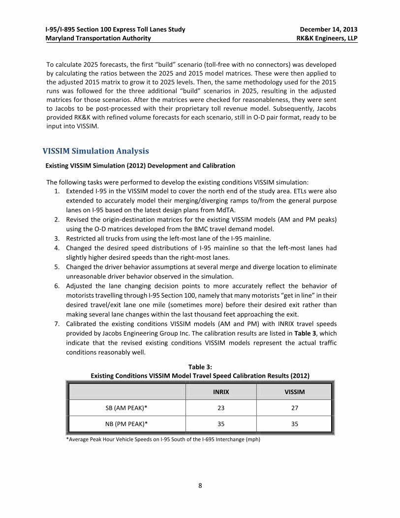
I-95/I-895 Section 100 Express Toll Lanes Study December 14, 2013 Maryland Transportation Authority RK&K Engineers, LLP
8
To calculate 2025 forecasts, the first “build” scenario (toll-free with no connectors) was developed by calculating the ratios between the 2025 and 2015 model matrices. These were then applied to the adjusted 2015 matrix to grow it to 2025 levels. Then, the same methodology used for the 2015 runs was followed for the three additional “build” scenarios in 2025, resulting in the adjusted matrices for those scenarios. After the matrices were checked for reasonableness, they were sent to Jacobs to be post-processed with their proprietary toll revenue model. Subsequently, Jacobs provided RK&K with refined volume forecasts for each scenario, still in O-D pair format, ready to be input into VISSIM.
VISSIM Simulation Analysis
Existing VISSIM Simulation (2012) Development and Calibration
The following tasks were performed to develop the existing conditions VISSIM simulation: 1. Extended I-95 in the VISSIM model to cover the north end of the study area. ETLs were also
extended to accurately model their merging/diverging ramps to/from the general purpose
lanes on I-95 based on the latest design plans from MdTA.
2. Revised the origin-destination matrices for the existing VISSIM models (AM and PM peaks)
using the O-D matrices developed from the BMC travel demand model.
3. Restricted all trucks from using the left-most lane of the I-95 mainline.
4. Changed the desired speed distributions of I-95 mainline so that the left-most lanes had
slightly higher desired speeds than the right-most lanes.
5. Changed the driver behavior assumptions at several merge and diverge location to eliminate
unreasonable driver behavior observed in the simulation.
6. Adjusted the lane changing decision points to more accurately reflect the behavior of
motorists travelling through I-95 Section 100, namely that many motorists “get in line” in their
desired travel/exit lane one mile (sometimes more) before their desired exit rather than
making several lane changes within the last thousand feet approaching the exit.
7. Calibrated the existing conditions VISSIM models (AM and PM) with INRIX travel speeds
provided by Jacobs Engineering Group Inc. The calibration results are listed in Table 3, which
indicate that the revised existing conditions VISSIM models represent the actual traffic
conditions reasonably well.
Table 3: Existing Conditions VISSIM Model Travel Speed Calibration Results (2012)
INRIX VISSIM
SB (AM PEAK)* 23 27
NB (PM PEAK)* 35 35
*Average Peak Hour Vehicle Speeds on I-95 South of the I-695 Interchange (mph)
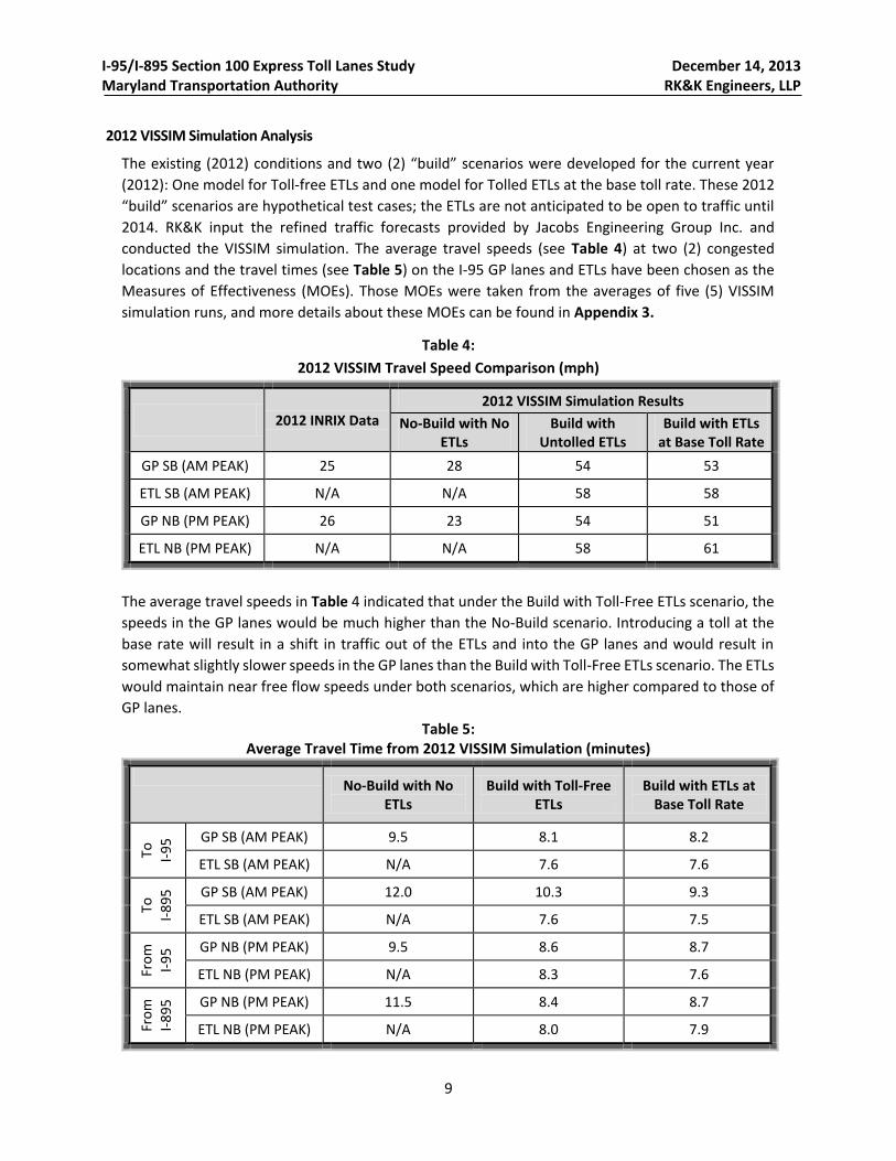
I-95/I-895 Section 100 Express Toll Lanes Study December 14, 2013 Maryland Transportation Authority RK&K Engineers, LLP
9
2012 VISSIM Simulation Analysis
The existing (2012) conditions and two (2) “build” scenarios were developed for the current year
(2012): One model for Toll-free ETLs and one model for Tolled ETLs at the base toll rate. These 2012
“build” scenarios are hypothetical test cases; the ETLs are not anticipated to be open to traffic until
2014. RK&K input the refined traffic forecasts provided by Jacobs Engineering Group Inc. and
conducted the VISSIM simulation. The average travel speeds (see Table 4) at two (2) congested
locations and the travel times (see Table 5) on the I-95 GP lanes and ETLs have been chosen as the
Measures of Effectiveness (MOEs). Those MOEs were taken from the averages of five (5) VISSIM
simulation runs, and more details about these MOEs can be found in Appendix 3.
Table 4:
2012 VISSIM Travel Speed Comparison (mph)
2012 INRIX Data
2012 VISSIM Simulation Results
No-Build with No ETLs
Build with Untolled ETLs
Build with ETLs at Base Toll Rate
GP SB (AM PEAK) 25 28 54 53
ETL SB (AM PEAK) N/A N/A 58 58
GP NB (PM PEAK) 26 23 54 51
ETL NB (PM PEAK) N/A N/A 58 61
The average travel speeds in Table 4 indicated that under the Build with Toll-Free ETLs scenario, the
speeds in the GP lanes would be much higher than the No-Build scenario. Introducing a toll at the
base rate will result in a shift in traffic out of the ETLs and into the GP lanes and would result in
somewhat slightly slower speeds in the GP lanes than the Build with Toll-Free ETLs scenario. The ETLs
would maintain near free flow speeds under both scenarios, which are higher compared to those of
GP lanes.
Table 5: Average Travel Time from 2012 VISSIM Simulation (minutes)
No-Build with No
ETLs Build with Toll-Free
ETLs Build with ETLs at
Base Toll Rate
To
I-9
5 GP SB (AM PEAK) 9.5 8.1 8.2
ETL SB (AM PEAK) N/A 7.6 7.6
To
I-8
95
GP SB (AM PEAK) 12.0 10.3 9.3
ETL SB (AM PEAK) N/A 7.6 7.5
Fro
m
I-9
5 GP NB (PM PEAK) 9.5 8.6 8.7
ETL NB (PM PEAK) N/A 8.3 7.6
Fro
m
I-8
95
GP NB (PM PEAK) 11.5 8.4 8.7
ETL NB (PM PEAK) N/A 8.0 7.9
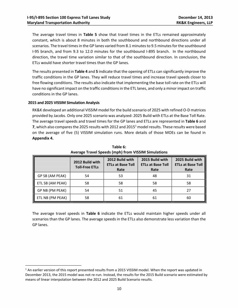
I-95/I-895 Section 100 Express Toll Lanes Study December 14, 2013 Maryland Transportation Authority RK&K Engineers, LLP
10
The average travel times in Table 5 show that travel times in the ETLs remained approximately
constant, which is about 8 minutes in both the southbound and northbound directions under all
scenarios. The travel times in the GP lanes varied from 8.1 minutes to 9.5 minutes for the southbound
I-95 branch, and from 9.3 to 12.0 minutes for the southbound I-895 branch. In the northbound
direction, the travel time variation similar to that of the southbound direction. In conclusion, the
ETLs would have shorter travel times than the GP lanes.
The results presented in Table 4 and 5 indicate that the opening of ETLs can significantly improve the
traffic conditions in the GP lanes. They will reduce travel times and increase travel speeds closer to
free flowing conditions. The results also indicate that implementing the base toll rate on the ETLs will
have no significant impact on the traffic conditions in the ETL lanes, and only a minor impact on traffic
conditions in the GP lanes.
2015 and 2025 VISSIM Simulation Analysis
RK&K developed an additional VISSIM model for the build scenario of 2025 with refined O-D matrices
provided by Jacobs. Only one 2025 scenario was analyzed: 2025 Build with ETLs at the Base Toll Rate.
The average travel speeds and travel times for the GP lanes and ETLs are represented in Table 6 and
7, which also compares the 2025 results with 2012 and 20151 model results. These results were based
on the average of five (5) VISSIM simulation runs. More details of those MOEs can be found in
Appendix 4.
Table 6: Average Travel Speeds (mph) from VISSIM Simulations
2012 Build with Toll-Free ETLs
2012 Build with ETLs at Base Toll
Rate
2015 Build with ETLs at Base Toll
Rate
2025 Build with ETLs at Base Toll
Rate
GP SB (AM PEAK) 54 53 48 31
ETL SB (AM PEAK) 58 58 58 58
GP NB (PM PEAK) 54 51 45 27
ETL NB (PM PEAK) 58 61 61 60
The average travel speeds in Table 6 indicate the ETLs would maintain higher speeds under all
scenarios than the GP lanes. The average speeds in the ETLs also demonstrate less variation than the
GP lanes.
1 An earlier version of this report presented results from a 2015 VISSIM model. When the report was updated in December 2013, the 2015 model was not re-run. Instead, the results for the 2015 Build scenario were estimated by means of linear interpolation between the 2012 and 2025 Build Scenario results.
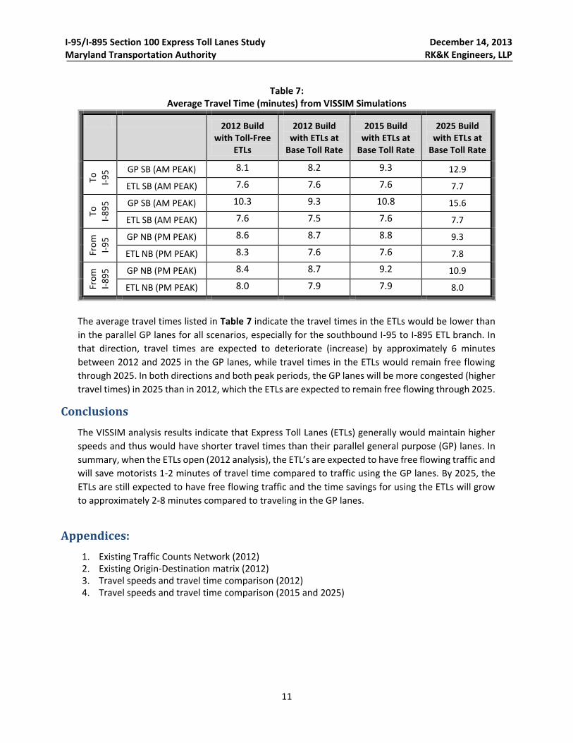
I-95/I-895 Section 100 Express Toll Lanes Study December 14, 2013 Maryland Transportation Authority RK&K Engineers, LLP
11
Table 7: Average Travel Time (minutes) from VISSIM Simulations
2012 Build with Toll-Free
ETLs
2012 Build with ETLs at
Base Toll Rate
2015 Build with ETLs at
Base Toll Rate
2025 Build with ETLs at
Base Toll Rate
To
I-9
5 GP SB (AM PEAK) 8.1 8.2 9.3 12.9
ETL SB (AM PEAK) 7.6 7.6 7.6 7.7
To
I-8
95
GP SB (AM PEAK) 10.3 9.3 10.8 15.6
ETL SB (AM PEAK) 7.6 7.5 7.6 7.7
Fro
m
I-9
5 GP NB (PM PEAK) 8.6 8.7 8.8 9.3
ETL NB (PM PEAK) 8.3 7.6 7.6 7.8
Fro
m
I-8
95
GP NB (PM PEAK) 8.4 8.7 9.2 10.9
ETL NB (PM PEAK) 8.0 7.9 7.9 8.0
The average travel times listed in Table 7 indicate the travel times in the ETLs would be lower than
in the parallel GP lanes for all scenarios, especially for the southbound I-95 to I-895 ETL branch. In
that direction, travel times are expected to deteriorate (increase) by approximately 6 minutes
between 2012 and 2025 in the GP lanes, while travel times in the ETLs would remain free flowing
through 2025. In both directions and both peak periods, the GP lanes will be more congested (higher
travel times) in 2025 than in 2012, which the ETLs are expected to remain free flowing through 2025.
Conclusions
The VISSIM analysis results indicate that Express Toll Lanes (ETLs) generally would maintain higher
speeds and thus would have shorter travel times than their parallel general purpose (GP) lanes. In
summary, when the ETLs open (2012 analysis), the ETL’s are expected to have free flowing traffic and
will save motorists 1-2 minutes of travel time compared to traffic using the GP lanes. By 2025, the
ETLs are still expected to have free flowing traffic and the time savings for using the ETLs will grow
to approximately 2-8 minutes compared to traveling in the GP lanes.
Appendices:
1. Existing Traffic Counts Network (2012) 2. Existing Origin-Destination matrix (2012) 3. Travel speeds and travel time comparison (2012) 4. Travel speeds and travel time comparison (2015 and 2025)

I-95 Section 100 ETL Study Traffic Counts Balanced w OD 2012 Existing No Build without I-695 Ramps
A(1) 2011 (4,700) 6,200 3,800 (6,700) F(5)
1.041 2004 (490) 1,030 910 (330)
2009 (5,150) 6,770 4,190 (7,705)
I-95
B(2)
2011 (1,030) 1,525 605 (1,860) 2010 (5,095) 6,610 4,270 (6,445) 2010 (435) 1,020 910 (330)
2010 (45) (480) (505) R 340 (915) 2010 (575) (4,220) (300) R 475 (860) 2010 (95) (340) 2010
(1,355) (1,345) 95 440 990 T 1,460 (1,070) (2,735) (2,975) (0) (2,735) 920 5,155 535 T 1,100 (1,110) (2,380) (2,435) (0) (2,380) 275 745 T 1,715 (1,765) (1,765) (1,763)
1,680 1,655 R T L L 710 (750) 2,510 2,580 0 2,510 R T L L 575 (410) 2,150 2,085 0 2,150 R T 1,715 1,713 I(7)
1,030 MD 43 975 (285) 90 L L T R 1,975 2,040 0 1,975 (615) 415 L L T R 1,665 MD 43 1,585 0 1,665 L T 1,195 1,184 MD 43
(1,510) (1,555) (1,140) 700 T 100 175 285 (2,430) (2,460) (0) (2,430) (1,135) 740 T 490 3,380 390 (2,140) (2,065) (0) (2,140) (1,520) 1,195 T 160 910 (1,520) (1,520)
C(3) (130) 185 R (230) (660) (785) (680) 820 R (1,050) (4,970) (705) (620) 470 R (520) (330)
(1,360) 1,335 560 (1,675) 3 (5,310) 6,550 4,260 (6,725) 2 (960) 1,215 1,070 (850) 1
Philadelphia Rd N(12)
D(4) Honeygo Blvd H(6, 21) Growing Rate for 4 year
1.03 2006 (1,425) 1,330 1,390 (1,520)
(465) (830) (130) R 115 (145)
G(50,51) (845) 480 780 70 T 80 (110) (480)
725 R T L L 110 (225) 305 P(14)
I-95 2010 575 (320) 300 L L T R 410 Golden Ring Center
(650) (170) 125 T 165 975 215 (650)
(158) 174 (160) 150 R (270) (1,055) (350)
(1,215) 1,040 1,355 (1,675) 6
L(10) (0) 0 0 (0) (0) 0 0 (0)
Philadelphia Rd
2010 (1,510) 1,885 1,305 (1,860)
2010 (1,480) 1,850 1,115 (1,795) 2010 (5,310) 6,550 4,260 (6,725) 2010 (845) 725 575 (650)
2011 (305) (715) (460) R 390 (1,030) 2007 (1,145) (3,265) (900) R 685 (1,330) 2010 (845) R 575 (650) 2010
(4,750) (4,590) 215 415 1,220 T 4,000 (4,050) (5,490) (4,980) (0) (5,490) 1,110 4,305 1,135 T 2,900 (2,425) (4,245) (4,595) (0) (4,245) 725 T 3,725 (3,400) (4,050) (4,050) (4,670)
5,010 4,425 R T L L 370 (410) 4,760 6,440 0 4,760 R T L L 865 (490) 4,450 4,065 0 4,450 R 4,300 4,300 3,775 O(13)
4,115 I-695 4,415 (235) 205 L L T R 5,655 4,255 0 5,655 (1,260) 935 L L T R 3,850 I-695 4,275 0 3,850 3,030 I-695 3,595 4,285 I-695
(4,990) (4,805) (4,300) 4,000 T 210 520 435 (5,190) (5,840) (0) (5,190) (2,965) 2,320 T 750 2,640 395 (4,415) (3,975) (0) (4,415) (3,520) 3,030 T (3,520) (4,115) (4,220)
J(8) (270) 210 R (235) (530) (430) (965) 2,400 R (1,920) (4,135) (550) (895) 820 R
(1,395) 995 1,165 (1,195) 4 (4,720) 7,570 3,785 (6,605) 5 (895) 820 8
2010 (1,425) 1,115 1,070 (1,640)
K(9) Belair Rd W(60, 61)
(0) 0 0 (0) (0) 0 0 (0)
V(20) 2012 (4,505) 7,120 3,870 (7,295)
2010 925 1,595 840 (1,335)
2012 (925) 1,595 1,300 (1,335) 2012 (4,720) 7,570 3,785 (6,605) (0) 0 2010 (1,215) 1,040 1,355 (1,675)
(250) (425) (250) R 900 (450) 2012 (1,750) (2,970) (800) (415)
(1,650) 550 895 150 T 1,850 (1,300) (1,750) (1,750) (0) (1,750) 2,750 4,820 665 375
2,600 R T L 2,750 2,750 0 2,750 R T T L
I-895 1,200 L T R 1,600 1,600 0 1,600 (2,900) 1,600 L I-95 T 820 (635) 575 L T R 565
Q(15) (1,950) (1,950) 1,200 T 200 400 250 (2,900) (2,900) (0) (2,900) 2,185 (895) 780 190 (595)
(100) (885) (700) (3,705) (260) 245 R (1,040) (180)
(425) 895 850 (1,685) 11 (2,970) 4,820 2,185 (3,705) 9 (1,060) 910 970 (1,220) 7
R(16) Moravia Rd M(11) Philadelphia Rd
(0) 0 0 (0)
(2,970) 4,820 2,185 (3,705)
2012 (2,970) 4,820 2,185 (3,705)
(2,970) 2012
(1,650) 4,820 T 1,180 (1,650) (1,950) (1,950)
S(17) 1,180 T L 745 (300) 1,925 1,925 U(19)
1,200 T R 1,580 1,580 Pulsaski HW
(2,115) (2,115) 1,200 T 2,185 380 (2,765) (2,765)
(3,705) (650)
(3,270) 5,565 2,565 (4,355) 10
T(18) I-95
(491) 399
RK&K Page 1 of 1 Date: 10/23/2012
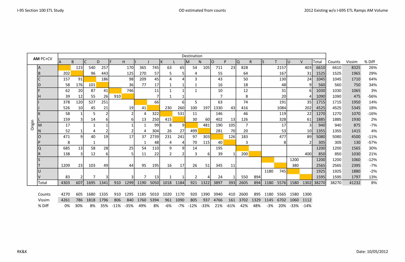
I‐95 Section 100 ETL Study OD estimated from counts 2012 Existing w/o I‐695 ETL Ramps AM Volume
A B C D F H I J K L M N O P Q R S T U V Total Counts Vissim % DiffA 123 540 257 170 365 745 63 65 54 105 711 23 828 2157 403 6610 6610 8325 26%
B 202 96 443 125 270 57 5 5 4 55 64 167 31 1525 1525 1965 29%
C 157 91 186 98 209 45 4 4 3 43 50 130 24 1045 1045 1710 64%
D 58 176 101 36 77 17 1 1 1 16 18 48 9 560 560 750 34%
F 62 20 87 41 746 11 1 1 1 10 12 31 6 1030 1030 1065 3%
H 39 12 55 26 910 7 1 1 7 8 20 4 1090 1090 475 -56%
I 378 120 527 251 66 6 5 63 74 191 35 1715 1715 1950 14%
J 526 10 45 21 19 41 230 260 100 197 1330 43 416 1084 202 4525 4525 5345 18%
K 58 1 5 2 2 4 322 531 11 146 46 119 22 1270 1270 1070 -16%
L 159 3 14 6 6 13 250 415 30 60 402 13 126 328 61 1885 1885 1930 2%
M 17 1 1 1 1 99 8 9 481 190 105 7 17 3 940 940 875 -7%
N 52 1 4 2 2 4 304 26 27 499 281 70 20 53 10 1355 1355 1415 4%
O 471 9 40 19 17 37 2739 231 241 97 303 126 183 477 89 5080 5080 4500 -11%
P 8 1 1 48 4 4 70 115 40 3 8 2 305 305 130 -57%
Q 685 13 58 28 25 54 110 9 9 14 195 1200 1200 1565 30%
R 138 3 12 6 5 11 22 2 2 3 6 39 1 200 400 850 850 1030 21%
S 1200 1200 1200 1060 -12%
T 1209 23 103 49 44 95 195 16 17 26 51 345 11 380 2565 2565 2395 -7%
U 1180 745 1925 1925 1880 -2%
V 83 2 7 3 3 7 13 1 1 2 4 24 1 550 894 1595 1595 1797 13%
Total 4303 607 1695 1341 910 1299 1190 5050 1018 1184 921 1322 3897 393 2605 894 1180 5576 1580 1302 38270 38270 41232 8%
Counts 4270 605 1680 1335 910 1295 1185 5010 1020 1170 920 1390 3940 410 2600 895 1180 5565 1580 1300Vissim 4261 786 1818 1796 806 840 1760 5394 961 1090 805 937 4766 161 3702 1329 1145 6702 1060 1112% Diff 0% 30% 8% 35% ‐11% ‐35% 49% 8% ‐6% ‐7% ‐12% ‐33% 21% ‐61% 42% 48% ‐3% 20% ‐33% ‐14%
AM PC+CVDestination
Orig
in
RK&K Date: 10/05/2012

I‐95 Section 100 ETL Study OD estimated from counts 2012 Existing w/o I‐695 ETL Ramps PM Volume
A B C D F H I J K L M N O P Q R S T U V Total Counts Vissim % DiffA 189 232 155 87 213 674 67 169 42 68 583 23 715 1632 247 5095 5095 5325 5%
B 128 45 481 69 168 23 2 6 1 19 24 55 8 1030 1030 1315 28%
C 290 286 131 157 382 51 5 13 3 44 54 125 19 1560 1560 1965 26%
D 199 662 231 107 261 35 3 9 2 30 37 85 13 1675 1675 2275 36%
F 53 24 29 19 341 4 1 3 4 10 1 490 490 500 2%
H 184 82 100 67 330 14 1 4 1 12 15 34 5 850 850 1505 77%
I 627 279 343 229 47 12 3 41 50 116 17 1765 1765 1815 3%
J 742 51 63 42 31 75 295 295 100 165 1406 55 212 484 73 4090 4090 5655 38%
K 93 6 8 5 4 9 286 542 12 177 27 60 9 1240 1240 1640 32%
L 98 7 8 6 4 10 335 714 13 22 185 7 28 64 10 1510 1510 1450 -4%
M 47 3 4 3 2 5 136 14 34 578 205 192 6 15 2 1245 1245 1250 0%
N 80 6 7 5 3 8 235 23 59 557 328 130 11 25 4 1480 1480 1575 6%
O 846 59 72 49 35 85 2479 246 621 102 323 172 116 266 40 5510 5510 4300 -22%
P 19 1 2 1 1 2 56 6 14 141 144 83 3 6 1 480 480 475 -1%
Q 937 65 80 53 38 94 125 12 31 34 480 1950 1950 3110 59%
R 324 22 28 18 13 33 43 4 11 12 19 166 6 100 886 1685 1685 1825 8%
S 2115 2115 2115 1800 -15%
T 1714 119 146 97 71 172 229 23 57 63 103 877 34 650 4355 4355 6600 52%
U 1650 300 1950 1950 1130 -42%
V 116 8 10 7 5 12 15 2 4 4 7 59 2 250 425 925 925 1150 24%
Total 6497 1870 1408 1367 330 969 1529 4787 1417 1882 1091 1429 4698 621 1652 425 1650 3277 2765 1335 41000 41000 46660 0.138
Counts 6445 1860 1400 1360 330 965 1520 4750 1425 1860 1090 1520 4735 650 1650 425 1650 3270 2765 1335Vissim 8493 2461 1806 1478 1030 869 2483 5450 1400 2550 982 1203 5193 366 1876 856 800 3455 2460 1449% Diff 32% 32% 29% 9% 212% ‐10% 63% 15% ‐2% 37% ‐10% ‐21% 10% ‐44% 14% 101% ‐52% 6% ‐11% 9%
PM PC+CVDestination
Orig
in
RK&K Date: 10/08/2012

I‐95 Section 100 ETL Study OD from VISSIM 2014 AM 2014 w/o I‐695 ETL Ramps
lAM PC+CV
DestinationA B C D F H I J K L M N O P Q R S T U V Total
A 194 570 311 189 486 267 46 83 53 46 456 11 1609 167 3511 327 8325B 181 140 775 96 247 247 4 7 5 27 147 1 20 13 51 3 1965B 181 140 775 96 247 247 4 7 5 27 147 1 20 13 51 3 1965C 225 125 285 119 306 306 5 9 6 33 182 1 25 16 63 4 1710D 69 200 150 37 94 94 1 3 2 10 56 0 8 5 19 1 750F 34 19 57 31 840 37 1 1 1 4 22 0 4 2 11 1 1065H 26 15 44 24 300 29 0 1 1 3 17 0 3 2 9 1 475I 291 169 495 270 320 5 9 6 35 191 1 38 18 97 6 1950J 590 243 265 230 2116 676 1225 5345K 46 1 4 2 1 4 290 440 8 18 121 2 39 5 81 8 1070K 46 1 4 2 1 4 290 440 8 18 121 2 39 5 81 8 1070L 148 61 250 465 530 169 307 1930M 32 1 3 1 1 2 140 7 12 350 250 25 15 2 31 3 875
Orig
in
N 69 2 6 3 2 5 302 14 26 530 280 65 32 4 67 7 1415O 337 174 139 2238 106 193 150 300 50 237 33 492 50 4500
O
P 4 0 0 0 0 0 20 1 2 20 55 20 2 0 4 0 130Q 815 22 65 36 23 63 323 15 28 10 21 143 2 1565R 67 2 5 3 2 5 25 1 2 1 2 11 0 205 700 1030R 67 2 5 3 2 5 25 1 2 1 2 11 0 205 700 1030S 1060 1060T 1263 34 100 54 34 97 484 23 42 14 32 214 3 2395U 1145 735 1880V 64 2 5 0 2 5 24 1 2 1 2 10 0 620 1060 1798Total 4261 786 1818 1796 300 1346 1760 5394 961 1090 805 937 4766 161 3702 1329 1145 6702 1060 1112 41233
RK&K Date: 10/08/2012
I‐95 Section 100 ETL Study OD from VISSIM 2014 PM 2014 w/o I‐695 ETL Ramps
lPM PC+CV
DestinationA B C D F H I J K L M N O P Q R S T U V Total
A 279 279 142 87 288 780 56 189 54 77 600 15 718 69 1546 147 5325B 139 115 650 59 196 30 2 7 2 3 23 1 26 3 55 5 1315B 139 115 650 59 196 30 2 7 2 3 23 1 26 3 55 5 1315C 333 425 225 141 469 71 5 17 5 7 55 1 62 6 131 13 1965D 278 850 325 118 392 59 4 14 4 6 46 1 52 5 110 10 2275F 48 27 27 14 350 7 0 2 0 1 5 0 6 1 12 1 500H 151 85 85 43 1030 21 1 5 1 2 16 0 18 2 39 4 1505I 577 326 326 166 79 6 19 5 8 61 2 70 7 149 14 1815J 1087 318 340 330 2640 331 609 5655K 77 8 8 4 2 8 240 1020 14 21 162 4 21 2 45 4 1640K 77 8 8 4 2 8 240 1020 14 21 162 4 21 2 45 4 1640L 103 30 275 705 248 31 58 1450M 59 6 6 3 2 6 120 9 29 550 325 100 10 1 22 2 1250
Orig
in
N 124 12 12 6 4 13 251 18 61 565 310 125 21 2 45 4 1575O 727 180 212 1638 118 398 175 275 100 140 14 294 28 4300
O
P 27 3 3 1 1 3 55 4 13 100 175 75 5 0 10 1 475Q 399 140 140 71 34 171 1501 43 353 18 26 207 5 3110R 56 22 22 11 6 26 97 7 24 3 4 212 1 120 1215 1825R 56 22 22 11 6 26 97 7 24 3 4 212 1 120 1215 1825S 1800 1800T 4289 271 271 137 63 341 196 79 60 34 48 141 10 660 6600U 800 330 1130V 19 7 7 4 2 9 31 2 8 1 1 69 0 245 745 1150Total 8493 2461 1806 1478 1030 869 2483 5450 1400 2550 982 1203 5193 366 1876 856 800 3455 2460 1449 46660
RK&K Date: 10/08/2012
I‐95 Section 100 ETL Study OD Matrix Comparison (AM) VISSIM 2014 ‐ Exising 2012
A B C D F H I J K L M N O P Q R S T U V TotalA 71 30 54 19 121 ‐478 ‐17 18 ‐1 ‐59 ‐255 ‐12 781 167 1354 ‐76 1715B ‐21 44 332 ‐29 ‐22 190 ‐1 2 1 27 92 1 ‐45 13 ‐116 ‐28 440C 67 34 99 21 97 261 1 5 3 33 139 1 ‐26 16 ‐67 ‐20 665D 11 24 49 1 17 77 0 2 1 10 40 0 ‐11 5 ‐29 ‐8 190F ‐29 ‐1 ‐30 ‐10 94 26 0 0 0 4 12 0 ‐8 2 ‐20 ‐5 35H ‐13 3 ‐11 ‐2 ‐610 22 ‐1 0 1 3 10 0 ‐5 2 ‐11 ‐3 ‐615I ‐87 48 ‐32 19 254 5 3 1 35 128 1 ‐36 18 ‐94 ‐29 235J 63 ‐10 ‐45 ‐21 ‐19 202 35 ‐30 ‐100 ‐197 786 ‐43 260 140 ‐202 820K ‐12 0 ‐1 0 ‐1 ‐1 ‐32 ‐91 ‐3 18 ‐25 2 ‐7 5 ‐39 ‐14 ‐200L ‐11 ‐3 ‐14 ‐6 ‐6 48 0 50 ‐30 ‐60 128 ‐13 43 ‐21 ‐61 45M 15 1 2 0 0 1 41 ‐1 3 ‐131 60 ‐80 8 2 14 0 ‐65N 17 1 2 1 1 ‐2 ‐12 ‐1 31 ‐1 ‐5 12 4 14 ‐3 60O ‐133 ‐9 134 ‐19 ‐17 102 ‐501 ‐125 ‐47 53 ‐3 ‐76 54 33 15 ‐38 ‐580P ‐4 0 ‐1 0 ‐1 ‐29 ‐3 ‐2 ‐50 ‐60 ‐20 ‐1 0 ‐4 ‐2 ‐175Q 130 9 8 8 ‐2 9 212 6 19 ‐5 21 ‐52 2 365R ‐71 ‐1 ‐7 ‐3 ‐3 ‐6 3 ‐1 0 ‐2 ‐4 ‐28 ‐1 5 300 180S ‐140 ‐140T 54 11 ‐3 5 ‐10 2 289 7 25 ‐12 ‐19 ‐131 ‐8 ‐380 ‐170U ‐35 ‐10 ‐45V ‐19 0 ‐2 ‐3 ‐1 ‐2 11 0 1 ‐1 ‐2 ‐14 ‐1 70 166 203Total ‐42 179 123 455 ‐610 47 570 344 ‐57 ‐94 ‐116 ‐385 869 ‐232 1097 435 ‐35 1126 ‐520 ‐190 2963
AM PC+CVDestination
Orig
in
RK&K Date: 10/08/2012
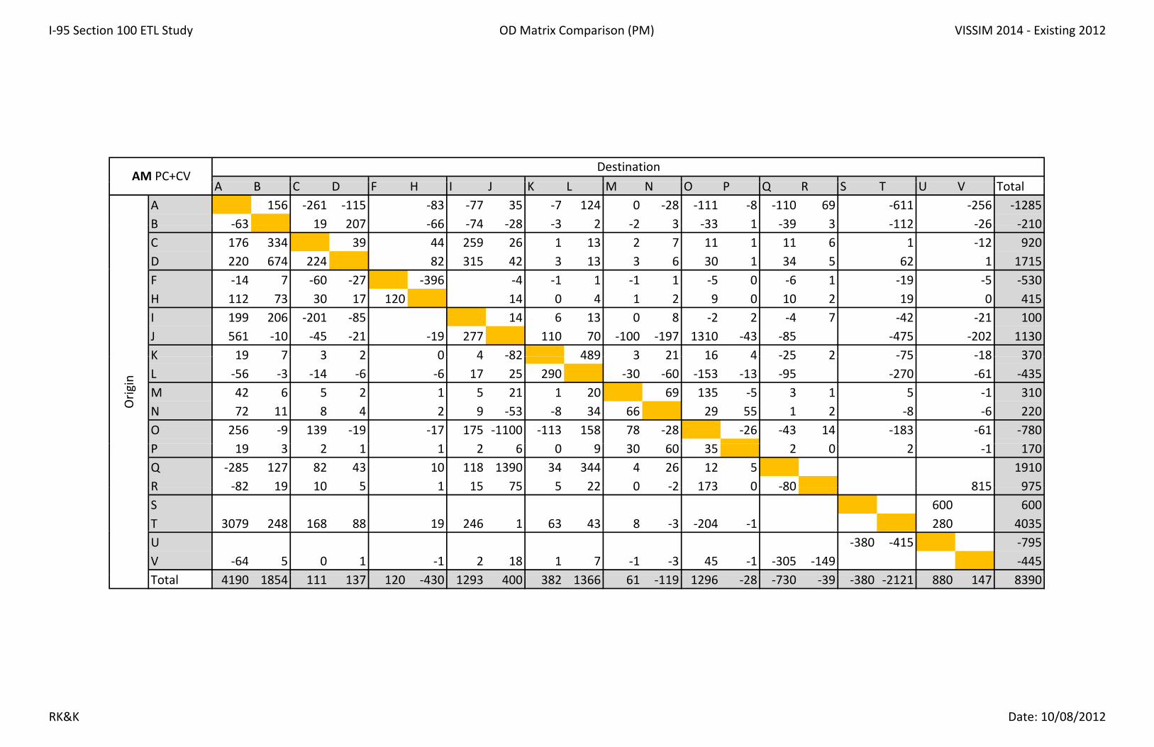
I‐95 Section 100 ETL Study OD Matrix Comparison (PM) VISSIM 2014 ‐ Existing 2012
lAM PC+CV
DestinationA B C D F H I J K L M N O P Q R S T U V Total
A 156 ‐261 ‐115 ‐83 ‐77 35 ‐7 124 0 ‐28 ‐111 ‐8 ‐110 69 ‐611 ‐256 ‐1285B ‐63 19 207 ‐66 ‐74 ‐28 ‐3 2 ‐2 3 ‐33 1 ‐39 3 ‐112 ‐26 ‐210B 63 19 207 66 74 28 3 2 2 3 33 1 39 3 112 26 210C 176 334 39 44 259 26 1 13 2 7 11 1 11 6 1 ‐12 920D 220 674 224 82 315 42 3 13 3 6 30 1 34 5 62 1 1715F ‐14 7 ‐60 ‐27 ‐396 ‐4 ‐1 1 ‐1 1 ‐5 0 ‐6 1 ‐19 ‐5 ‐530H 112 73 30 17 120 14 0 4 1 2 9 0 10 2 19 0 415I 199 206 ‐201 ‐85 14 6 13 0 8 ‐2 2 ‐4 7 ‐42 ‐21 100J 561 ‐10 ‐45 ‐21 ‐19 277 110 70 ‐100 ‐197 1310 ‐43 ‐85 ‐475 ‐202 1130K 19 7 3 2 0 4 ‐82 489 3 21 16 4 ‐25 2 ‐75 ‐18 370K 19 7 3 2 0 4 82 489 3 21 16 4 25 2 75 18 370L ‐56 ‐3 ‐14 ‐6 ‐6 17 25 290 ‐30 ‐60 ‐153 ‐13 ‐95 ‐270 ‐61 ‐435M 42 6 5 2 1 5 21 1 20 69 135 ‐5 3 1 5 ‐1 310
Orig
in
N 72 11 8 4 2 9 ‐53 ‐8 34 66 29 55 1 2 ‐8 ‐6 220O 256 ‐9 139 ‐19 ‐17 175 ‐1100 ‐113 158 78 ‐28 ‐26 ‐43 14 ‐183 ‐61 ‐780
O
P 19 3 2 1 1 2 6 0 9 30 60 35 2 0 2 ‐1 170Q ‐285 127 82 43 10 118 1390 34 344 4 26 12 5 1910R ‐82 19 10 5 1 15 75 5 22 0 ‐2 173 0 ‐80 815 975R ‐82 19 10 5 1 15 75 5 22 0 ‐2 173 0 ‐80 815 975S 600 600T 3079 248 168 88 19 246 1 63 43 8 ‐3 ‐204 ‐1 280 4035U ‐380 ‐415 ‐795V ‐64 5 0 1 ‐1 2 18 1 7 ‐1 ‐3 45 ‐1 ‐305 ‐149 ‐445Total 4190 1854 111 137 120 ‐430 1293 400 382 1366 61 ‐119 1296 ‐28 ‐730 ‐39 ‐380 ‐2121 880 147 8390
RK&K Date: 10/08/2012
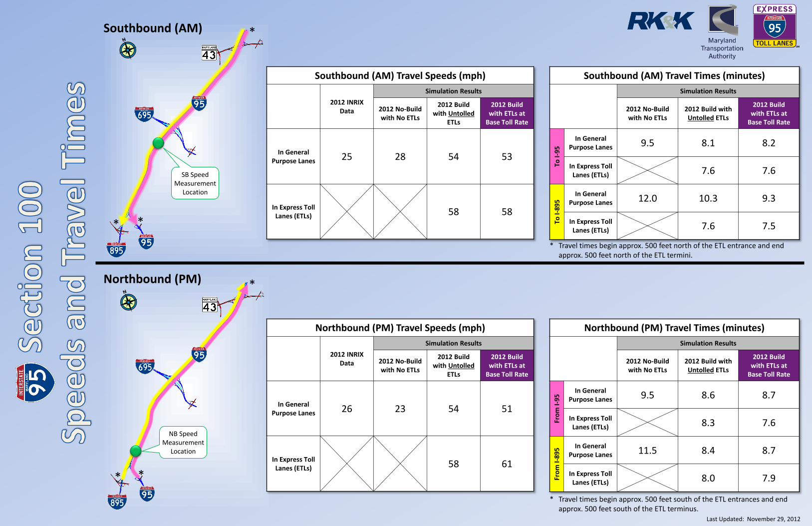
Last Updated: November 29, 2012
Southbound (AM)
Northbound (PM)
Southbound (AM) Travel Times (minutes)
Simulation Results
2012 No-Buildwith No ETLs
2012 Build withUntolled ETLs
2012 Buildwith ETLs at
Base Toll Rate
To I-
95
In General Purpose Lanes 9.5 8.1 8.2
In Express Toll Lanes (ETLs) 7.6 7.6
To I-
89
5
In General Purpose Lanes 12.0 10.3 9.3
In Express Toll Lanes (ETLs) 7.6 7.5
Southbound (AM) Travel Speeds (mph)
2012 INRIX Data
Simulation Results
2012 No-Build with No ETLs
2012 Build with Untolled
ETLs
2012 Build with ETLs at
Base Toll Rate
In GeneralPurpose Lanes 25 28 54 53
In Express Toll Lanes (ETLs) 58 58
* Travel times begin approx. 500 feet north of the ETL entrance and end approx. 500 feet north of the ETL termini.
**
*
* Travel times begin approx. 500 feet south of the ETL entrances and end approx. 500 feet south of the ETL terminus.
**
*
SB Speed Measurement
Location
NB Speed Measurement
Location
Northbound (PM) Travel Speeds (mph)
2012 INRIX Data
Simulation Results
2012 No-Build with No ETLs
2012 Build with Untolled
ETLs
2012 Build with ETLs at
Base Toll Rate
In GeneralPurpose Lanes 26 23 54 51
In Express Toll Lanes (ETLs) 58 61
Northbound (PM) Travel Times (minutes)
Simulation Results
2012 No-Buildwith No ETLs
2012 Build withUntolled ETLs
2012 Buildwith ETLs at
Base Toll Rate
Fro
m I-
95
In General Purpose Lanes 9.5 8.6 8.7
In Express Toll Lanes (ETLs) 8.3 7.6
Fro
m I-
89
5 In General Purpose Lanes 11.5 8.4 8.7
In Express Toll Lanes (ETLs) 8.0 7.9
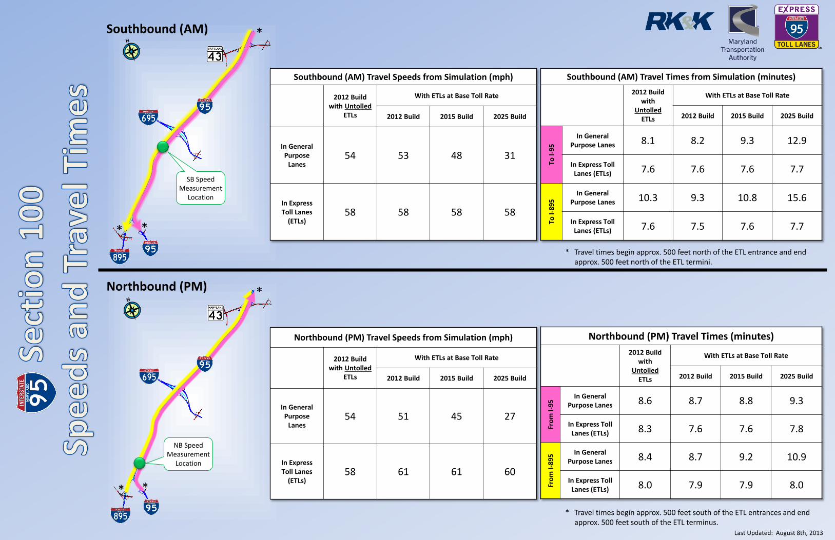
Last Updated: August 8th, 2013
Southbound (AM)
Northbound (PM)
Southbound (AM) Travel Times from Simulation (minutes)
2012 Build with
UntolledETLs
With ETLs at Base Toll Rate
2012 Build 2015 Build 2025 Build
To I-
95
In General Purpose Lanes 8.1 8.2 9.3 12.9
In Express Toll Lanes (ETLs) 7.6 7.6 7.6 7.7
To I-
89
5
In General Purpose Lanes 10.3 9.3 10.8 15.6
In Express Toll Lanes (ETLs) 7.6 7.5 7.6 7.7
Southbound (AM) Travel Speeds from Simulation (mph)
2012 Build with Untolled
ETLs
With ETLs at Base Toll Rate
2012 Build 2015 Build 2025 Build
In GeneralPurpose
Lanes54 53 48 31
In Express Toll Lanes
(ETLs)58 58 58 58
* Travel times begin approx. 500 feet north of the ETL entrance and end approx. 500 feet north of the ETL termini.
**
*
* Travel times begin approx. 500 feet south of the ETL entrances and end approx. 500 feet south of the ETL terminus.
**
*
SB Speed Measurement
Location
NB Speed Measurement
Location
Northbound (PM) Travel Speeds from Simulation (mph)
2012 Build with Untolled
ETLs
With ETLs at Base Toll Rate
2012 Build 2015 Build 2025 Build
In GeneralPurpose
Lanes54 51 45 27
In Express Toll Lanes
(ETLs)58 61 61 60
Northbound (PM) Travel Times (minutes)
2012 Build with
UntolledETLs
With ETLs at Base Toll Rate
2012 Build 2015 Build 2025 Build
Fro
m I-
95
In General Purpose Lanes 8.6 8.7 8.8 9.3
In Express Toll Lanes (ETLs) 8.3 7.6 7.6 7.8
Fro
m I-
89
5 In General Purpose Lanes 8.4 8.7 9.2 10.9
In Express Toll Lanes (ETLs) 8.0 7.9 7.9 8.0

APPENDIX C
Toll Sensitivity Analyses

Time Period Southbound Northbound
Night (Weekday and Weekend) 6 pm to 5 am 8 pm to 6 am
Weekday Peak (Mon‐Thurs) 6 am to 8:30 am 3 pm to 7 pm
Weekday Peak (Fri) 6 am to 8:30 am 3 pm to 7 pm
Weekday Off‐Peak 5 am to 6 am; 8:30 am to 6 pm 6 am to 3 pm; 7pm to 8 pm
Weekend Peak (Sat) 5 am to 12 pm; 2 pm to 6 pm 5 am to 12 pm; 2 pm to 8 pm
Weekend Off‐Peak (Sat) 12 pm to 2 pm 12 pm to 2 pm
Weekend Peak (Sun) 5 am to 2 pm; 5 pm to 6 pm 5 am to 2 pm; 5 pm to 8 pm
Weekend Off‐Peak (Sun) 2 pm to 5 pm 2 pm to 5 pm
MDTA I‐95 ETL T&R Study
2015 Toll Sensitivity Graphs
Time Period Definition by Day and Direction
I‐95 ETL TStudy
2015 Toll Sensitivity Graphs
Page 1 of 8
JACOBS
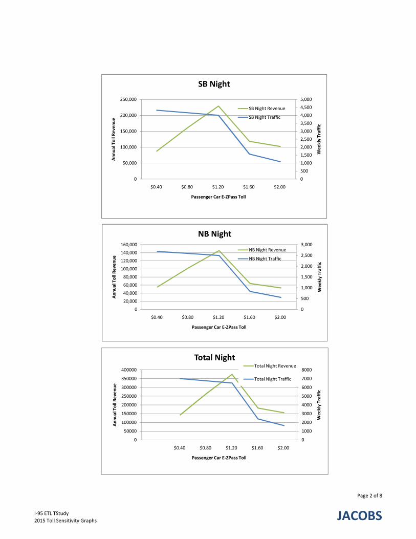
0
500
1,000
1,500
2,000
2,500
3,000
3,500
4,000
4,500
5,000
0
50,000
100,000
150,000
200,000
250,000
$0.40 $0.80 $1.20 $1.60 $2.00
Weekly Traffic
Annual Toll Reven
ue
Passenger Car E‐ZPass Toll
SB Night
SB Night Revenue
SB Night Traffic
1,000
1,500
2,000
2,500
3,000
60,000
80,000
100,000
120,000
140,000
160,000
Weekly Traffic
ual Toll Reven
ue
NB Night
NB Night Revenue
NB Night Traffic
0
500
1,000
1,500
2,000
2,500
3,000
3,500
4,000
4,500
5,000
0
50,000
100,000
150,000
200,000
250,000
$0.40 $0.80 $1.20 $1.60 $2.00
Weekly Traffic
Annual Toll Reven
ue
Passenger Car E‐ZPass Toll
SB Night
SB Night Revenue
SB Night Traffic
0
500
1,000
1,500
2,000
2,500
3,000
0
20,000
40,000
60,000
80,000
100,000
120,000
140,000
160,000
$0.40 $0.80 $1.20 $1.60 $2.00 Weekly Traffic
Annual Toll Reven
ue
Passenger Car E‐ZPass Toll
NB Night
NB Night Revenue
NB Night Traffic
0
1000
2000
3000
4000
5000
6000
7000
8000
0
50000
100000
150000
200000
250000
300000
350000
400000
$0.40 $0.80 $1.20 $1.60 $2.00
Weekly Traffic
Annual Toll Reven
ue
Passenger Car E‐ZPass Toll
Total NightTotal Night Revenue
Total Night Traffic
I‐95 ETL TStudy
2015 Toll Sensitivity Graphs
Page 2 of 8
JACOBS

0
2,000
4,000
6,000
8,000
10,000
12,000
14,000
16,000
18,000
20,000
0
200,000
400,000
600,000
800,000
1,000,000
1,200,000
1,400,000
1,600,000
1,800,000
2,000,000
$0.40
$0.80
$1.20
$1.60
$2.00
$2.40
$2.80
$3.20
$3.60
$4.00
$4.40
$4.80
$5.20
$5.60
$6.00
$6.40
$6.80
$7.20
$7.60
$8.00
Weekly Traffic
Annual Toll Reven
ue
Passenger Car E‐ZPass Toll
SB Weekday Peak
SB Weekday Peak Revenue
SB Weekday Peak Traffic
10 000
15,000
20,000
25,000
1 000 000
1,500,000
2,000,000
2,500,000
ekly Traffic
Toll Reven
ue
NB Weekday Peak
NB Weekday Peak RevenueNB Weekday Peak Traffic
0
2,000
4,000
6,000
8,000
10,000
12,000
14,000
16,000
18,000
20,000
0
200,000
400,000
600,000
800,000
1,000,000
1,200,000
1,400,000
1,600,000
1,800,000
2,000,000
$0.40
$0.80
$1.20
$1.60
$2.00
$2.40
$2.80
$3.20
$3.60
$4.00
$4.40
$4.80
$5.20
$5.60
$6.00
$6.40
$6.80
$7.20
$7.60
$8.00
Weekly Traffic
Annual Toll Reven
ue
Passenger Car E‐ZPass Toll
SB Weekday Peak
SB Weekday Peak Revenue
SB Weekday Peak Traffic
0
5,000
10,000
15,000
20,000
25,000
0
500,000
1,000,000
1,500,000
2,000,000
2,500,000
$0.40
$0.80
$1.20
$1.60
$2.00
$2.40
$2.80
$3.20
$3.60
$4.00
$4.40
$4.80
$5.20
$5.60
$6.00
$6.40
$6.80
$7.20
$7.60
$8.00
Weekly Traffic
Annual Toll Reven
ue
Passenger Car E‐ZPass Toll
NB Weekday Peak
NB Weekday Peak RevenueNB Weekday Peak Traffic
0
5,000
10,000
15,000
20,000
25,000
30,000
35,000
40,000
0
500,000
1,000,000
1,500,000
2,000,000
2,500,000
3,000,000
3,500,000
4,000,000
4,500,000
$0.40
$0.80
$1.20
$1.60
$2.00
$2.40
$2.80
$3.20
$3.60
$4.00
$4.40
$4.80
$5.20
$5.60
$6.00
$6.40
$6.80
$7.20
$7.60
$8.00
Weekly Traffic
Annual Toll Reven
ue
Passenger Car E‐ZPass Toll
Total Weekday Peak
Total Weekday Peak Revenue
Total Weekday Peak Traffic
I‐95 ETL TStudy
2015 Toll Sensitivity Graphs
Page 3 of 8
JACOBS

3,000
4,000
5,000
6,000
7,000
8,000
600,000
800,000
1,000,000
1,200,000
1,400,000
eekly Traffic
al Toll Reven
ue
NB Friday Peak
NB Friday Peak
0
1,000
2,000
3,000
4,000
5,000
6,000
7,000
8,000
0
200,000
400,000
600,000
800,000
1,000,000
1,200,000
1,400,000
$0.40
$0.80
$1.20
$1.60
$2.00
$2.40
$2.80
$3.20
$3.60
$4.00
$4.40
$4.80
$5.20
$5.60
$6.00
$6.40
$6.80
$7.20
$7.60
$8.00
Weekly Traffic
Annual Toll Reven
ue
Passenger Car E‐ZPass Toll
NB Friday Peak
NB Friday Peak RevenueNB Friday Peak Traffic
I‐95 ETL TStudy
2015 Toll Sensitivity Graphs
Page 4 of 8
JACOBS
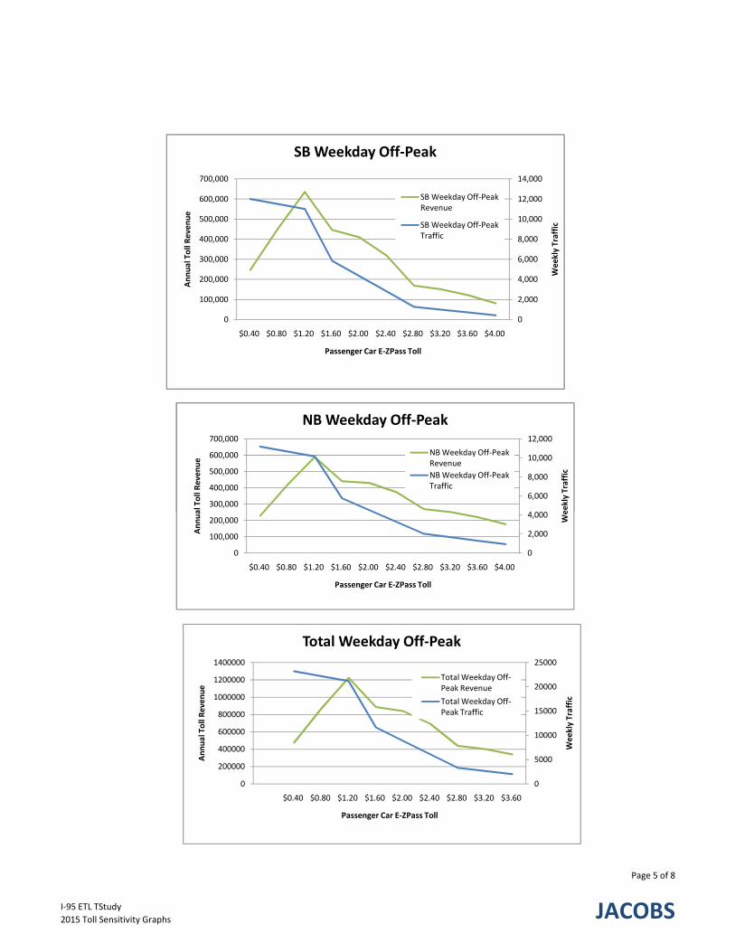
0
2,000
4,000
6,000
8,000
10,000
12,000
14,000
0
100,000
200,000
300,000
400,000
500,000
600,000
700,000
$0.40 $0.80 $1.20 $1.60 $2.00 $2.40 $2.80 $3.20 $3.60 $4.00
Weekly Traffic
Annual Toll Reven
ue
Passenger Car E‐ZPass Toll
SB Weekday Off‐Peak
SB Weekday Off‐Peak Revenue
SB Weekday Off‐Peak Traffic
6,000
8,000
10,000
12,000
300,000
400,000
500,000
600,000
700,000
eekly Traffic
al Toll Reven
ue
NB Weekday Off‐Peak
NB Weekday Off‐Peak Revenue
NB Weekday Off‐Peak Traffic
0
2,000
4,000
6,000
8,000
10,000
12,000
14,000
0
100,000
200,000
300,000
400,000
500,000
600,000
700,000
$0.40 $0.80 $1.20 $1.60 $2.00 $2.40 $2.80 $3.20 $3.60 $4.00
Weekly Traffic
Annual Toll Reven
ue
Passenger Car E‐ZPass Toll
SB Weekday Off‐Peak
SB Weekday Off‐Peak Revenue
SB Weekday Off‐Peak Traffic
0
2,000
4,000
6,000
8,000
10,000
12,000
0
100,000
200,000
300,000
400,000
500,000
600,000
700,000
$0.40 $0.80 $1.20 $1.60 $2.00 $2.40 $2.80 $3.20 $3.60 $4.00 Weekly Traffic
Annual Toll Reven
ue
Passenger Car E‐ZPass Toll
NB Weekday Off‐Peak
NB Weekday Off‐Peak Revenue
NB Weekday Off‐Peak Traffic
0
5000
10000
15000
20000
25000
0
200000
400000
600000
800000
1000000
1200000
1400000
$0.40 $0.80 $1.20 $1.60 $2.00 $2.40 $2.80 $3.20 $3.60
Weekly Traffic
Annual Toll Reven
ue
Passenger Car E‐ZPass Toll
Total Weekday Off‐Peak
Total Weekday Off‐Peak Revenue
Total Weekday Off‐Peak Traffic
I‐95 ETL TStudy
2015 Toll Sensitivity Graphs
Page 5 of 8
JACOBS
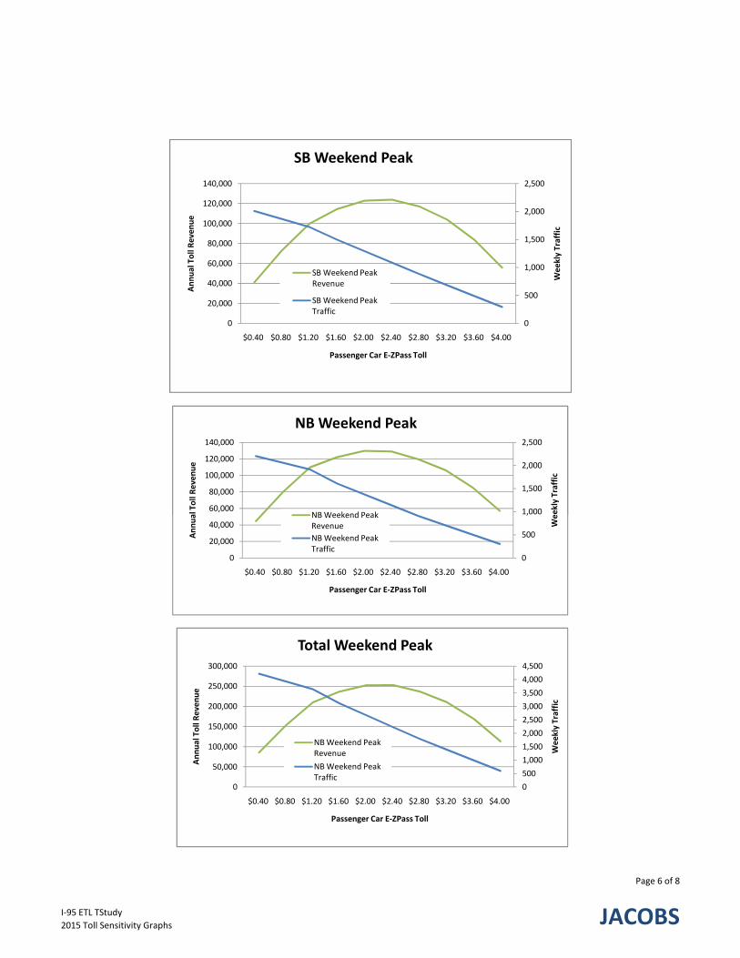
0
500
1,000
1,500
2,000
2,500
0
20,000
40,000
60,000
80,000
100,000
120,000
140,000
$0.40 $0.80 $1.20 $1.60 $2.00 $2.40 $2.80 $3.20 $3.60 $4.00
Weekly Traffic
Annual Toll Reven
ue
Passenger Car E‐ZPass Toll
SB Weekend Peak
SB Weekend Peak Revenue
SB Weekend Peak Traffic
1,000
1,500
2,000
2,500
60,000
80,000
100,000
120,000
140,000
ekly Traffic
al Toll Reven
ue
NB Weekend Peak
NBWeekend Peak
0
500
1,000
1,500
2,000
2,500
0
20,000
40,000
60,000
80,000
100,000
120,000
140,000
$0.40 $0.80 $1.20 $1.60 $2.00 $2.40 $2.80 $3.20 $3.60 $4.00
Weekly Traffic
Annual Toll Reven
ue
Passenger Car E‐ZPass Toll
SB Weekend Peak
SB Weekend Peak Revenue
SB Weekend Peak Traffic
0
500
1,000
1,500
2,000
2,500
0
20,000
40,000
60,000
80,000
100,000
120,000
140,000
$0.40 $0.80 $1.20 $1.60 $2.00 $2.40 $2.80 $3.20 $3.60 $4.00
Weekly Traffic
Annual Toll Reven
ue
Passenger Car E‐ZPass Toll
NB Weekend Peak
NB Weekend Peak Revenue
NB Weekend Peak Traffic
0
500
1,000
1,500
2,000
2,500
3,000
3,500
4,000
4,500
0
50,000
100,000
150,000
200,000
250,000
300,000
$0.40 $0.80 $1.20 $1.60 $2.00 $2.40 $2.80 $3.20 $3.60 $4.00
Weekly Traffic
Annual Toll Reven
ue
Passenger Car E‐ZPass Toll
Total Weekend Peak
NB Weekend Peak Revenue
NB Weekend Peak Traffic
I‐95 ETL TStudy
2015 Toll Sensitivity Graphs
Page 6 of 8
JACOBS
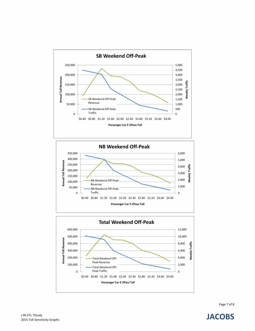
0
500
1,000
1,500
2,000
2,500
3,000
3,500
4,000
4,500
5,000
0
50,000
100,000
150,000
200,000
250,000
$0.40 $0.80 $1.20 $1.60 $2.00 $2.40 $2.80 $3.20 $3.60 $4.00
Weekly Traffic
Annual Toll Reven
ue
Passenger Car E‐ZPass Toll
SB Weekend Off‐Peak
SB Weekend Off‐Peak Revenue
SB Weekend Off‐Peak Traffic
3,000
4,000
5,000
6,000
150,000
200,000
250,000
300,000
350,000
ekly Traffic
l Toll Reven
ue
NB Weekend Off‐Peak
0
500
1,000
1,500
2,000
2,500
3,000
3,500
4,000
4,500
5,000
0
50,000
100,000
150,000
200,000
250,000
$0.40 $0.80 $1.20 $1.60 $2.00 $2.40 $2.80 $3.20 $3.60 $4.00
Weekly Traffic
Annual Toll Reven
ue
Passenger Car E‐ZPass Toll
SB Weekend Off‐Peak
SB Weekend Off‐Peak Revenue
SB Weekend Off‐Peak Traffic
0
1,000
2,000
3,000
4,000
5,000
6,000
0
50,000
100,000
150,000
200,000
250,000
300,000
350,000
$0.40 $0.80 $1.20 $1.60 $2.00 $2.40 $2.80 $3.20 $3.60 $4.00
Weekly Traffic
Annual Toll Reven
ue
Passenger Car E‐ZPass Toll
NB Weekend Off‐Peak
NB Weekend Off‐Peak Revenue
NB Weekend Off‐Peak Traffic
0
2,000
4,000
6,000
8,000
10,000
12,000
0
100,000
200,000
300,000
400,000
500,000
600,000
$0.40 $0.80 $1.20 $1.60 $2.00 $2.40 $2.80 $3.20 $3.60 $4.00
Weekly Traffic
Annual Toll Reven
ue
Passenger Car E‐ZPass Toll
Total Weekend Off‐Peak
Total Weekend Off‐Peak Revenue
Total Weekend Off‐Peak Traffic
I‐95 ETL TStudy
2015 Toll Sensitivity Graphs
Page 7 of 8
JACOBS
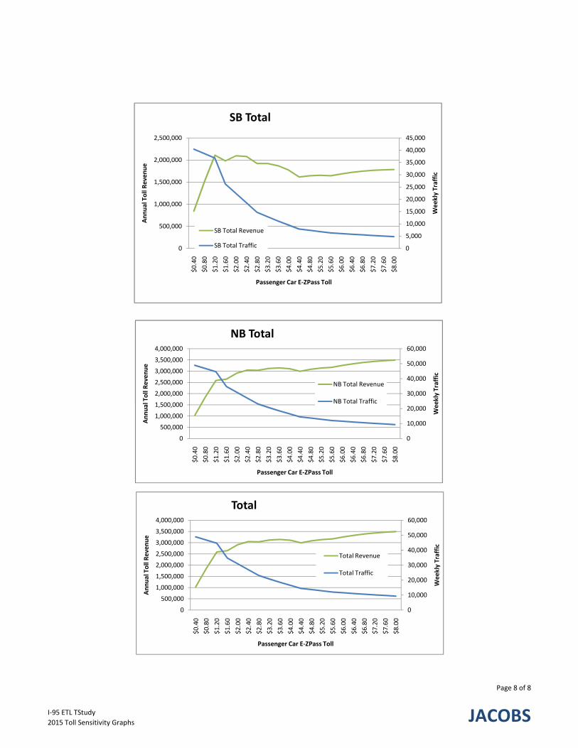
0
5,000
10,000
15,000
20,000
25,000
30,000
35,000
40,000
45,000
0
500,000
1,000,000
1,500,000
2,000,000
2,500,000
$0.40
$0.80
$1.20
$1.60
$2.00
$2.40
$2.80
$3.20
$3.60
$4.00
$4.40
$4.80
$5.20
$5.60
$6.00
$6.40
$6.80
$7.20
$7.60
$8.00
Weekly Traffic
Annual Toll Reven
ue
Passenger Car E‐ZPass Toll
SB Total
SB Total Revenue
SB Total Traffic
30,000
40,000
50,000
60,000
2,000,000
2,500,000
3,000,000
3,500,000
4,000,000
ekly Traffic
Toll Reven
ue
NB Total
NB Total Revenue
NB Total Traffic
0
5,000
10,000
15,000
20,000
25,000
30,000
35,000
40,000
45,000
0
500,000
1,000,000
1,500,000
2,000,000
2,500,000
$0.40
$0.80
$1.20
$1.60
$2.00
$2.40
$2.80
$3.20
$3.60
$4.00
$4.40
$4.80
$5.20
$5.60
$6.00
$6.40
$6.80
$7.20
$7.60
$8.00
Weekly Traffic
Annual Toll Reven
ue
Passenger Car E‐ZPass Toll
SB Total
SB Total Revenue
SB Total Traffic
0
10,000
20,000
30,000
40,000
50,000
60,000
0
500,000
1,000,000
1,500,000
2,000,000
2,500,000
3,000,000
3,500,000
4,000,000
$0.40
$0.80
$1.20
$1.60
$2.00
$2.40
$2.80
$3.20
$3.60
$4.00
$4.40
$4.80
$5.20
$5.60
$6.00
$6.40
$6.80
$7.20
$7.60
$8.00
Weekly Traffic
Annual Toll Reven
ue
Passenger Car E‐ZPass Toll
NB Total
NB Total Revenue
NB Total Traffic
0
10,000
20,000
30,000
40,000
50,000
60,000
0
500,000
1,000,000
1,500,000
2,000,000
2,500,000
3,000,000
3,500,000
4,000,000
$0.40
$0.80
$1.20
$1.60
$2.00
$2.40
$2.80
$3.20
$3.60
$4.00
$4.40
$4.80
$5.20
$5.60
$6.00
$6.40
$6.80
$7.20
$7.60
$8.00
Weekly Traffic
Annual Toll Reven
ue
Passenger Car E‐ZPass Toll
Total
Total Revenue
Total Traffic
I‐95 ETL TStudy
2015 Toll Sensitivity Graphs
Page 8 of 8
JACOBS
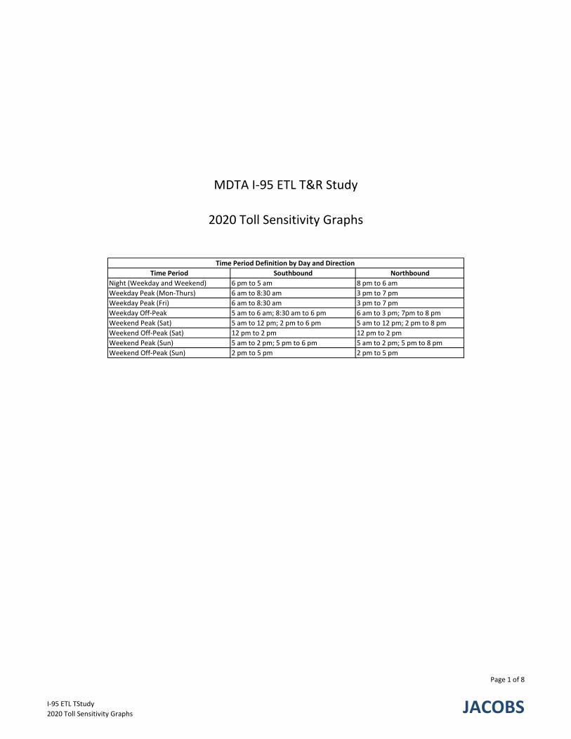
Time Period Southbound Northbound
Night (Weekday and Weekend) 6 pm to 5 am 8 pm to 6 am
Weekday Peak (Mon‐Thurs) 6 am to 8:30 am 3 pm to 7 pm
Weekday Peak (Fri) 6 am to 8:30 am 3 pm to 7 pm
Weekday Off‐Peak 5 am to 6 am; 8:30 am to 6 pm 6 am to 3 pm; 7pm to 8 pm
Weekend Peak (Sat) 5 am to 12 pm; 2 pm to 6 pm 5 am to 12 pm; 2 pm to 8 pm
Weekend Off‐Peak (Sat) 12 pm to 2 pm 12 pm to 2 pm
Weekend Peak (Sun) 5 am to 2 pm; 5 pm to 6 pm 5 am to 2 pm; 5 pm to 8 pm
Weekend Off‐Peak (Sun) 2 pm to 5 pm 2 pm to 5 pm
MDTA I‐95 ETL T&R Study
2020 Toll Sensitivity Graphs
Time Period Definition by Day and Direction
I‐95 ETL TStudy
2020 Toll Sensitivity Graphs
Page 1 of 8
JACOBS
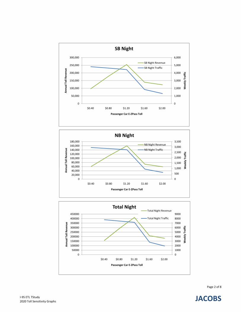
0
1,000
2,000
3,000
4,000
5,000
6,000
0
50,000
100,000
150,000
200,000
250,000
300,000
$0.40 $0.80 $1.20 $1.60 $2.00
Weekly Traffic
Annual Toll Reven
ue
Passenger Car E‐ZPass Toll
SB Night
SB Night Revenue
SB Night Traffic
1 000
1,500
2,000
2,500
3,000
3,500
60,000
80,000
100,000
120,000
140,000
160,000
180,000
Weekly Traffic
ual Toll Reven
ue
NB Night
NB Night Revenue
NB Night Traffic
0
1,000
2,000
3,000
4,000
5,000
6,000
0
50,000
100,000
150,000
200,000
250,000
300,000
$0.40 $0.80 $1.20 $1.60 $2.00
Weekly Traffic
Annual Toll Reven
ue
Passenger Car E‐ZPass Toll
SB Night
SB Night Revenue
SB Night Traffic
0
500
1,000
1,500
2,000
2,500
3,000
3,500
0
20,000
40,000
60,000
80,000
100,000
120,000
140,000
160,000
180,000
$0.40 $0.80 $1.20 $1.60 $2.00 Weekly Traffic
Annual Toll Reven
ue
Passenger Car E‐ZPass Toll
NB Night
NB Night Revenue
NB Night Traffic
0
1000
2000
3000
4000
5000
6000
7000
8000
9000
0
50000
100000
150000
200000
250000
300000
350000
400000
450000
$0.40 $0.80 $1.20 $1.60 $2.00
Weekly Traffic
Annual Toll Reven
ue
Passenger Car E‐ZPass Toll
Total NightTotal Night Revenue
Total Night Traffic
I‐95 ETL TStudy
2020 Toll Sensitivity Graphs
Page 2 of 8
JACOBS
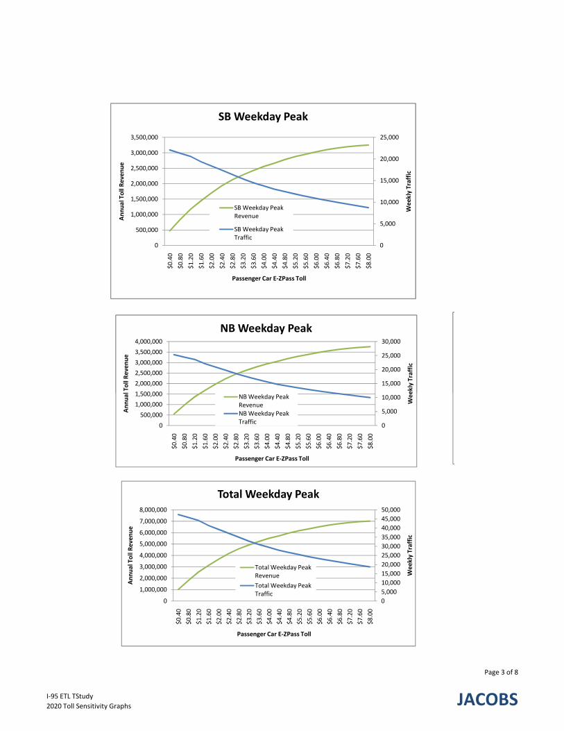
0
5,000
10,000
15,000
20,000
25,000
0
500,000
1,000,000
1,500,000
2,000,000
2,500,000
3,000,000
3,500,000
$0.40
$0.80
$1.20
$1.60
$2.00
$2.40
$2.80
$3.20
$3.60
$4.00
$4.40
$4.80
$5.20
$5.60
$6.00
$6.40
$6.80
$7.20
$7.60
$8.00
Weekly Traffic
Annual Toll Reven
ue
Passenger Car E‐ZPass Toll
SB Weekday Peak
SB Weekday Peak Revenue
SB Weekday Peak Traffic
15,000
20,000
25,000
30,000
1 500 000
2,000,000
2,500,000
3,000,000
3,500,000
4,000,000
ekly Traffic
Toll Reven
ue
NB Weekday Peak
0
5,000
10,000
15,000
20,000
25,000
0
500,000
1,000,000
1,500,000
2,000,000
2,500,000
3,000,000
3,500,000
$0.40
$0.80
$1.20
$1.60
$2.00
$2.40
$2.80
$3.20
$3.60
$4.00
$4.40
$4.80
$5.20
$5.60
$6.00
$6.40
$6.80
$7.20
$7.60
$8.00
Weekly Traffic
Annual Toll Reven
ue
Passenger Car E‐ZPass Toll
SB Weekday Peak
SB Weekday Peak Revenue
SB Weekday Peak Traffic
0
5,000
10,000
15,000
20,000
25,000
30,000
0
500,000
1,000,000
1,500,000
2,000,000
2,500,000
3,000,000
3,500,000
4,000,000
$0.40
$0.80
$1.20
$1.60
$2.00
$2.40
$2.80
$3.20
$3.60
$4.00
$4.40
$4.80
$5.20
$5.60
$6.00
$6.40
$6.80
$7.20
$7.60
$8.00
Weekly Traffic
Annual Toll Reven
ue
Passenger Car E‐ZPass Toll
NB Weekday Peak
NB Weekday Peak RevenueNB Weekday Peak Traffic
0
5,000
10,000
15,000
20,000
25,000
30,000
35,000
40,000
45,000
50,000
0
1,000,000
2,000,000
3,000,000
4,000,000
5,000,000
6,000,000
7,000,000
8,000,000
$0.40
$0.80
$1.20
$1.60
$2.00
$2.40
$2.80
$3.20
$3.60
$4.00
$4.40
$4.80
$5.20
$5.60
$6.00
$6.40
$6.80
$7.20
$7.60
$8.00
Weekly Traffic
Annual Toll Reven
ue
Passenger Car E‐ZPass Toll
Total Weekday Peak
Total Weekday Peak Revenue
Total Weekday Peak Traffic
I‐95 ETL TStudy
2020 Toll Sensitivity Graphs
Page 3 of 8
JACOBS
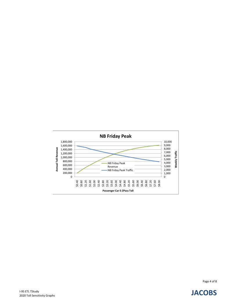
4,0005,0006,0007,0008,0009,00010,000
600 000
800,000
1,000,000
1,200,000
1,400,000
1,600,000
1,800,000
eekly Traffic
al Toll Reven
ue
NB Friday Peak
NB Friday Peak
01,0002,0003,0004,0005,0006,0007,0008,0009,00010,000
0
200,000
400,000
600,000
800,000
1,000,000
1,200,000
1,400,000
1,600,000
1,800,000
$0.40
$0.80
$1.20
$1.60
$2.00
$2.40
$2.80
$3.20
$3.60
$4.00
$4.40
$4.80
$5.20
$5.60
$6.00
$6.40
$6.80
$7.20
$7.60
$8.00
Weekly Traffic
Annual Toll Reven
ue
Passenger Car E‐ZPass Toll
NB Friday Peak
NB Friday Peak RevenueNB Friday Peak Traffic
I‐95 ETL TStudy
2020 Toll Sensitivity Graphs
Page 4 of 8
JACOBS
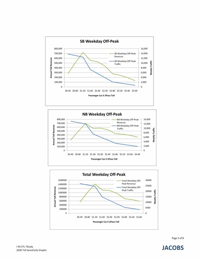
0
2,000
4,000
6,000
8,000
10,000
12,000
14,000
16,000
0
100,000
200,000
300,000
400,000
500,000
600,000
700,000
800,000
$0.40 $0.80 $1.20 $1.60 $2.00 $2.40 $2.80 $3.20 $3.60 $4.00
Weekly Traffic
Annual Toll Reven
ue
Passenger Car E‐ZPass Toll
SB Weekday Off‐Peak
SB Weekday Off‐Peak Revenue
SB Weekday Off‐Peak Traffic
6,000
8,000
10,000
12,000
14,000
300 000
400,000
500,000
600,000
700,000
800,000
eekly Traffic
al Toll Reven
ue
NB Weekday Off‐PeakNB Weekday Off‐Peak Revenue
NB Weekday Off‐Peak Traffic
0
2,000
4,000
6,000
8,000
10,000
12,000
14,000
16,000
0
100,000
200,000
300,000
400,000
500,000
600,000
700,000
800,000
$0.40 $0.80 $1.20 $1.60 $2.00 $2.40 $2.80 $3.20 $3.60 $4.00
Weekly Traffic
Annual Toll Reven
ue
Passenger Car E‐ZPass Toll
SB Weekday Off‐Peak
SB Weekday Off‐Peak Revenue
SB Weekday Off‐Peak Traffic
0
2,000
4,000
6,000
8,000
10,000
12,000
14,000
0
100,000
200,000
300,000
400,000
500,000
600,000
700,000
800,000
$0.40 $0.80 $1.20 $1.60 $2.00 $2.40 $2.80 $3.20 $3.60 $4.00 Weekly Traffic
Annual Toll Reven
ue
Passenger Car E‐ZPass Toll
NB Weekday Off‐PeakNB Weekday Off‐Peak Revenue
NB Weekday Off‐Peak Traffic
0
5000
10000
15000
20000
25000
30000
0
200000
400000
600000
800000
1000000
1200000
1400000
1600000
$0.40 $0.80 $1.20 $1.60 $2.00 $2.40 $2.80 $3.20 $3.60
Weekly Traffic
Annual Toll Reven
ue
Passenger Car E‐ZPass Toll
Total Weekday Off‐Peak
Total Weekday Off‐Peak Revenue
Total Weekday Off‐Peak Traffic
I‐95 ETL TStudy
2020 Toll Sensitivity Graphs
Page 5 of 8
JACOBS

0
500
1,000
1,500
2,000
2,500
3,000
0
20,000
40,000
60,000
80,000
100,000
120,000
140,000
160,000
180,000
$0.40 $0.80 $1.20 $1.60 $2.00 $2.40 $2.80 $3.20 $3.60 $4.00
Weekly Traffic
Annual Toll Reven
ue
Passenger Car E‐ZPass Toll
SB Weekend Peak
SB Weekend Peak Revenue
SB Weekend Peak Traffic
1,500
2,000
2,500
3,000
80,000
100,000
120,000
140,000
160,000
180,000
ekly Traffic
al Toll Reven
ue
NB Weekend Peak
NBWeekend Peak
0
500
1,000
1,500
2,000
2,500
3,000
0
20,000
40,000
60,000
80,000
100,000
120,000
140,000
160,000
180,000
$0.40 $0.80 $1.20 $1.60 $2.00 $2.40 $2.80 $3.20 $3.60 $4.00
Weekly Traffic
Annual Toll Reven
ue
Passenger Car E‐ZPass Toll
SB Weekend Peak
SB Weekend Peak Revenue
SB Weekend Peak Traffic
0
500
1,000
1,500
2,000
2,500
3,000
0
20,000
40,000
60,000
80,000
100,000
120,000
140,000
160,000
180,000
$0.40 $0.80 $1.20 $1.60 $2.00 $2.40 $2.80 $3.20 $3.60 $4.00
Weekly Traffic
Annual Toll Reven
ue
Passenger Car E‐ZPass Toll
NB Weekend Peak
NB Weekend Peak Revenue
NB Weekend Peak Traffic
0
1,000
2,000
3,000
4,000
5,000
6,000
0
50,000
100,000
150,000
200,000
250,000
300,000
350,000
$0.40 $0.80 $1.20 $1.60 $2.00 $2.40 $2.80 $3.20 $3.60 $4.00
Weekly Traffic
Annual Toll Reven
ue
Passenger Car E‐ZPass Toll
Total Weekend Peak
NB Weekend Peak Revenue
NB Weekend Peak Traffic
I‐95 ETL TStudy
2020 Toll Sensitivity Graphs
Page 6 of 8
JACOBS
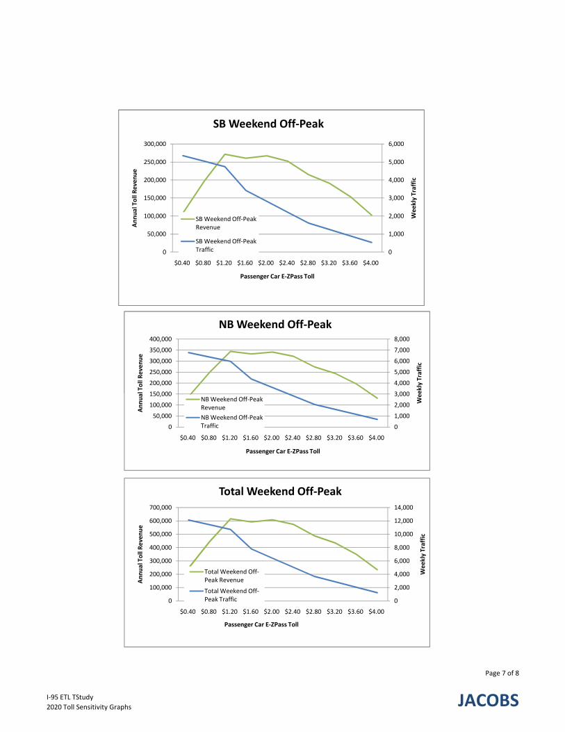
0
1,000
2,000
3,000
4,000
5,000
6,000
0
50,000
100,000
150,000
200,000
250,000
300,000
$0.40 $0.80 $1.20 $1.60 $2.00 $2.40 $2.80 $3.20 $3.60 $4.00
Weekly Traffic
Annual Toll Reven
ue
Passenger Car E‐ZPass Toll
SB Weekend Off‐Peak
SB Weekend Off‐Peak Revenue
SB Weekend Off‐Peak Traffic
3 000
4,000
5,000
6,000
7,000
8,000
150 000
200,000
250,000
300,000
350,000
400,000
ekly Traffic
l Toll Reven
ue
NB Weekend Off‐Peak
0
1,000
2,000
3,000
4,000
5,000
6,000
0
50,000
100,000
150,000
200,000
250,000
300,000
$0.40 $0.80 $1.20 $1.60 $2.00 $2.40 $2.80 $3.20 $3.60 $4.00
Weekly Traffic
Annual Toll Reven
ue
Passenger Car E‐ZPass Toll
SB Weekend Off‐Peak
SB Weekend Off‐Peak Revenue
SB Weekend Off‐Peak Traffic
0
1,000
2,000
3,000
4,000
5,000
6,000
7,000
8,000
0
50,000
100,000
150,000
200,000
250,000
300,000
350,000
400,000
$0.40 $0.80 $1.20 $1.60 $2.00 $2.40 $2.80 $3.20 $3.60 $4.00
Weekly Traffic
Annual Toll Reven
ue
Passenger Car E‐ZPass Toll
NB Weekend Off‐Peak
NB Weekend Off‐Peak Revenue
NB Weekend Off‐Peak Traffic
0
2,000
4,000
6,000
8,000
10,000
12,000
14,000
0
100,000
200,000
300,000
400,000
500,000
600,000
700,000
$0.40 $0.80 $1.20 $1.60 $2.00 $2.40 $2.80 $3.20 $3.60 $4.00
Weekly Traffic
Annual Toll Reven
ue
Passenger Car E‐ZPass Toll
Total Weekend Off‐Peak
Total Weekend Off‐Peak Revenue
Total Weekend Off‐Peak Traffic
I‐95 ETL TStudy
2020 Toll Sensitivity Graphs
Page 7 of 8
JACOBS
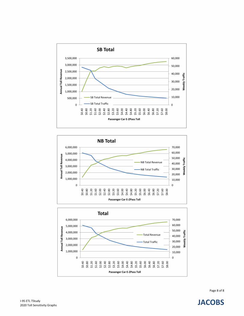
0
10,000
20,000
30,000
40,000
50,000
60,000
0
500,000
1,000,000
1,500,000
2,000,000
2,500,000
3,000,000
3,500,000
$0.40
$0.80
$1.20
$1.60
$2.00
$2.40
$2.80
$3.20
$3.60
$4.00
$4.40
$4.80
$5.20
$5.60
$6.00
$6.40
$6.80
$7.20
$7.60
$8.00
Weekly Traffic
Annual Toll Reven
ue
Passenger Car E‐ZPass Toll
SB Total
SB Total Revenue
SB Total Traffic
30,000
40,000
50,000
60,000
70,000
3,000,000
4,000,000
5,000,000
6,000,000
ekly Traffic
Toll Reven
ue
NB Total
NB Total Revenue
NB Total Traffic
0
10,000
20,000
30,000
40,000
50,000
60,000
0
500,000
1,000,000
1,500,000
2,000,000
2,500,000
3,000,000
3,500,000
$0.40
$0.80
$1.20
$1.60
$2.00
$2.40
$2.80
$3.20
$3.60
$4.00
$4.40
$4.80
$5.20
$5.60
$6.00
$6.40
$6.80
$7.20
$7.60
$8.00
Weekly Traffic
Annual Toll Reven
ue
Passenger Car E‐ZPass Toll
SB Total
SB Total Revenue
SB Total Traffic
0
10,000
20,000
30,000
40,000
50,000
60,000
70,000
0
1,000,000
2,000,000
3,000,000
4,000,000
5,000,000
6,000,000
$0.40
$0.80
$1.20
$1.60
$2.00
$2.40
$2.80
$3.20
$3.60
$4.00
$4.40
$4.80
$5.20
$5.60
$6.00
$6.40
$6.80
$7.20
$7.60
$8.00
Weekly Traffic
Annual Toll Reven
ue
Passenger Car E‐ZPass Toll
NB Total
NB Total Revenue
NB Total Traffic
0
10,000
20,000
30,000
40,000
50,000
60,000
70,000
0
1,000,000
2,000,000
3,000,000
4,000,000
5,000,000
6,000,000
$0.40
$0.80
$1.20
$1.60
$2.00
$2.40
$2.80
$3.20
$3.60
$4.00
$4.40
$4.80
$5.20
$5.60
$6.00
$6.40
$6.80
$7.20
$7.60
$8.00
Weekly Traffic
Annual Toll Reven
ue
Passenger Car E‐ZPass Toll
Total
Total Revenue
Total Traffic
I‐95 ETL TStudy
2020 Toll Sensitivity Graphs
Page 8 of 8
JACOBS

Time Period Southbound Northbound
Night (Weekday and Weekend) 6 pm to 5 am 8 pm to 6 am
Weekday Peak (Mon‐Thurs) 6 am to 8:30 am 3 pm to 7 pm
Weekday Peak (Fri) 6 am to 8:30 am 3 pm to 7 pm
Weekday Off‐Peak 5 am to 6 am; 8:30 am to 6 pm 6 am to 3 pm; 7pm to 8 pm
Weekend Peak (Sat) 5 am to 12 pm; 2 pm to 6 pm 5 am to 12 pm; 2 pm to 8 pm
Weekend Off‐Peak (Sat) 12 pm to 2 pm 12 pm to 2 pm
Weekend Peak (Sun) 5 am to 2 pm; 5 pm to 6 pm 5 am to 2 pm; 5 pm to 8 pm
Weekend Off‐Peak (Sun) 2 pm to 5 pm 2 pm to 5 pm
MDTA I‐95 ETL T&R Study
2025 Toll Sensitivity Graphs
Time Period Definition by Day and Direction
I‐95 ETL TStudy
2025 Toll Sensitivity Graphs
Page 1 of 8
JACOBS
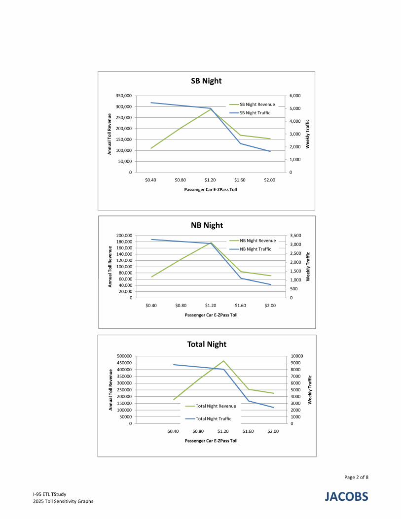
0
1,000
2,000
3,000
4,000
5,000
6,000
0
50,000
100,000
150,000
200,000
250,000
300,000
350,000
$0.40 $0.80 $1.20 $1.60 $2.00
Weekly Traffic
Annual Toll Reven
ue
Passenger Car E‐ZPass Toll
SB Night
SB Night Revenue
SB Night Traffic
1 000
1,500
2,000
2,500
3,000
3,500
60 000
80,000
100,000
120,000
140,000
160,000
180,000
200,000
Weekly Traffic
ual Toll Reven
ue
NB Night
NB Night Revenue
NB Night Traffic
0
1,000
2,000
3,000
4,000
5,000
6,000
0
50,000
100,000
150,000
200,000
250,000
300,000
350,000
$0.40 $0.80 $1.20 $1.60 $2.00
Weekly Traffic
Annual Toll Reven
ue
Passenger Car E‐ZPass Toll
SB Night
SB Night Revenue
SB Night Traffic
0
500
1,000
1,500
2,000
2,500
3,000
3,500
0
20,000
40,000
60,000
80,000
100,000
120,000
140,000
160,000
180,000
200,000
$0.40 $0.80 $1.20 $1.60 $2.00 Weekly Traffic
Annual Toll Reven
ue
Passenger Car E‐ZPass Toll
NB Night
NB Night Revenue
NB Night Traffic
0
1000
2000
3000
4000
5000
6000
7000
8000
9000
10000
0
50000
100000
150000
200000
250000
300000
350000
400000
450000
500000
$0.40 $0.80 $1.20 $1.60 $2.00
Weekly Traffic
Annual Toll Reven
ue
Passenger Car E‐ZPass Toll
Total Night
Total Night Revenue
Total Night Traffic
I‐95 ETL TStudy
2025 Toll Sensitivity Graphs
Page 2 of 8
JACOBS
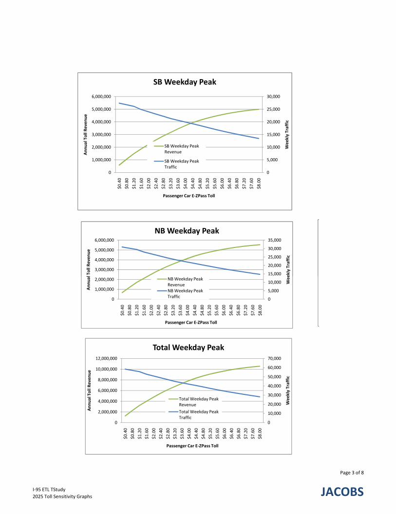
0
5,000
10,000
15,000
20,000
25,000
30,000
0
1,000,000
2,000,000
3,000,000
4,000,000
5,000,000
6,000,000
$0.40
$0.80
$1.20
$1.60
$2.00
$2.40
$2.80
$3.20
$3.60
$4.00
$4.40
$4.80
$5.20
$5.60
$6.00
$6.40
$6.80
$7.20
$7.60
$8.00
Weekly Traffic
Annual Toll Reven
ue
Passenger Car E‐ZPass Toll
SB Weekday Peak
SB Weekday Peak Revenue
SB Weekday Peak Traffic
15,000
20,000
25,000
30,000
35,000
3,000,000
4,000,000
5,000,000
6,000,000
ekly Traffic
Toll Reven
ue
NB Weekday Peak
0
5,000
10,000
15,000
20,000
25,000
30,000
0
1,000,000
2,000,000
3,000,000
4,000,000
5,000,000
6,000,000
$0.40
$0.80
$1.20
$1.60
$2.00
$2.40
$2.80
$3.20
$3.60
$4.00
$4.40
$4.80
$5.20
$5.60
$6.00
$6.40
$6.80
$7.20
$7.60
$8.00
Weekly Traffic
Annual Toll Reven
ue
Passenger Car E‐ZPass Toll
SB Weekday Peak
SB Weekday Peak Revenue
SB Weekday Peak Traffic
0
5,000
10,000
15,000
20,000
25,000
30,000
35,000
0
1,000,000
2,000,000
3,000,000
4,000,000
5,000,000
6,000,000
$0.40
$0.80
$1.20
$1.60
$2.00
$2.40
$2.80
$3.20
$3.60
$4.00
$4.40
$4.80
$5.20
$5.60
$6.00
$6.40
$6.80
$7.20
$7.60
$8.00
Weekly Traffic
Annual Toll Reven
ue
Passenger Car E‐ZPass Toll
NB Weekday Peak
NB Weekday Peak RevenueNB Weekday Peak Traffic
0
10,000
20,000
30,000
40,000
50,000
60,000
70,000
0
2,000,000
4,000,000
6,000,000
8,000,000
10,000,000
12,000,000
$0.40
$0.80
$1.20
$1.60
$2.00
$2.40
$2.80
$3.20
$3.60
$4.00
$4.40
$4.80
$5.20
$5.60
$6.00
$6.40
$6.80
$7.20
$7.60
$8.00
Weekly Traffic
Annual Toll Reven
ue
Passenger Car E‐ZPass Toll
Total Weekday Peak
Total Weekday Peak Revenue
Total Weekday Peak Traffic
I‐95 ETL TStudy
2025 Toll Sensitivity Graphs
Page 3 of 8
JACOBS
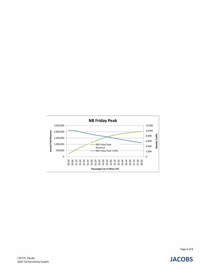
4 000
6,000
8,000
10,000
12,000
1,000,000
1,500,000
2,000,000
2,500,000
eekly Traffic
al Toll Reven
ue
NB Friday Peak
NB Friday Peak
0
2,000
4,000
6,000
8,000
10,000
12,000
0
500,000
1,000,000
1,500,000
2,000,000
2,500,000
$0.40
$0.80
$1.20
$1.60
$2.00
$2.40
$2.80
$3.20
$3.60
$4.00
$4.40
$4.80
$5.20
$5.60
$6.00
$6.40
$6.80
$7.20
$7.60
$8.00
Weekly Traffic
Annual Toll Reven
ue
Passenger Car E‐ZPass Toll
NB Friday Peak
NB Friday Peak RevenueNB Friday Peak Traffic
I‐95 ETL TStudy
2025 Toll Sensitivity Graphs
Page 4 of 8
JACOBS
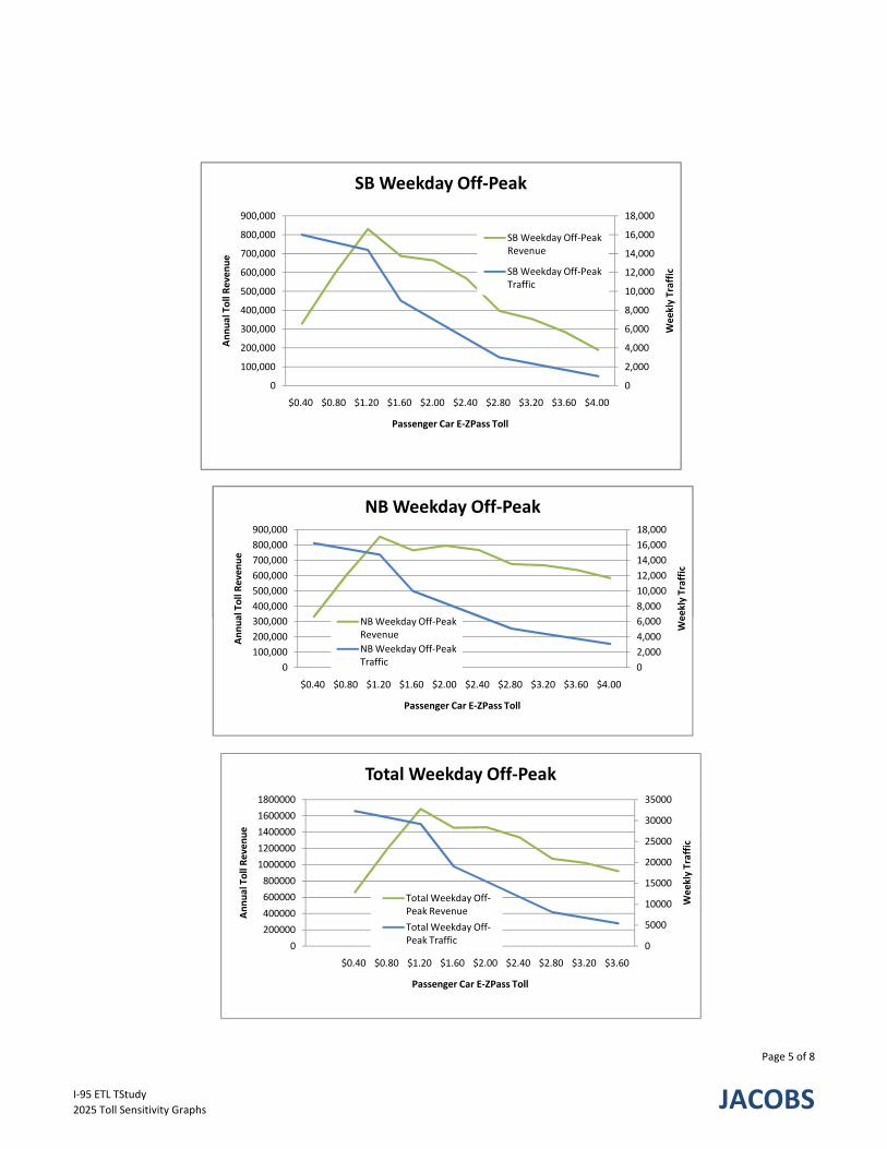
0
2,000
4,000
6,000
8,000
10,000
12,000
14,000
16,000
18,000
0
100,000
200,000
300,000
400,000
500,000
600,000
700,000
800,000
900,000
$0.40 $0.80 $1.20 $1.60 $2.00 $2.40 $2.80 $3.20 $3.60 $4.00
Weekly Traffic
Annual Toll Reven
ue
Passenger Car E‐ZPass Toll
SB Weekday Off‐Peak
SB Weekday Off‐Peak Revenue
SB Weekday Off‐Peak Traffic
8,000
10,000
12,000
14,000
16,000
18,000
400,000
500,000
600,000
700,000
800,000
900,000
eekly Traffic
al Toll Reven
ue
NB Weekday Off‐Peak
0
2,000
4,000
6,000
8,000
10,000
12,000
14,000
16,000
18,000
0
100,000
200,000
300,000
400,000
500,000
600,000
700,000
800,000
900,000
$0.40 $0.80 $1.20 $1.60 $2.00 $2.40 $2.80 $3.20 $3.60 $4.00
Weekly Traffic
Annual Toll Reven
ue
Passenger Car E‐ZPass Toll
SB Weekday Off‐Peak
SB Weekday Off‐Peak Revenue
SB Weekday Off‐Peak Traffic
0
2,000
4,000
6,000
8,000
10,000
12,000
14,000
16,000
18,000
0
100,000
200,000
300,000
400,000
500,000
600,000
700,000
800,000
900,000
$0.40 $0.80 $1.20 $1.60 $2.00 $2.40 $2.80 $3.20 $3.60 $4.00 Weekly Traffic
Annual Toll Reven
ue
Passenger Car E‐ZPass Toll
NB Weekday Off‐Peak
NB Weekday Off‐Peak Revenue
NB Weekday Off‐Peak Traffic
0
5000
10000
15000
20000
25000
30000
35000
0
200000
400000
600000
800000
1000000
1200000
1400000
1600000
1800000
$0.40 $0.80 $1.20 $1.60 $2.00 $2.40 $2.80 $3.20 $3.60
Weekly Traffic
Annual Toll Reven
ue
Passenger Car E‐ZPass Toll
Total Weekday Off‐Peak
Total Weekday Off‐Peak Revenue
Total Weekday Off‐Peak Traffic
I‐95 ETL TStudy
2025 Toll Sensitivity Graphs
Page 5 of 8
JACOBS
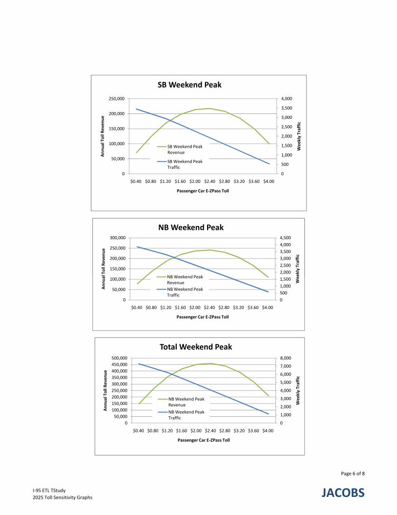
0
500
1,000
1,500
2,000
2,500
3,000
3,500
4,000
0
50,000
100,000
150,000
200,000
250,000
$0.40 $0.80 $1.20 $1.60 $2.00 $2.40 $2.80 $3.20 $3.60 $4.00
Weekly Traffic
Annual Toll Reven
ue
Passenger Car E‐ZPass Toll
SB Weekend Peak
SB Weekend Peak Revenue
SB Weekend Peak Traffic
2,000
2,500
3,000
3,500
4,000
4,500
150,000
200,000
250,000
300,000
ekly Traffic
al Toll Reven
ue
NB Weekend Peak
NBWeekend Peak
0
500
1,000
1,500
2,000
2,500
3,000
3,500
4,000
0
50,000
100,000
150,000
200,000
250,000
$0.40 $0.80 $1.20 $1.60 $2.00 $2.40 $2.80 $3.20 $3.60 $4.00
Weekly Traffic
Annual Toll Reven
ue
Passenger Car E‐ZPass Toll
SB Weekend Peak
SB Weekend Peak Revenue
SB Weekend Peak Traffic
0
500
1,000
1,500
2,000
2,500
3,000
3,500
4,000
4,500
0
50,000
100,000
150,000
200,000
250,000
300,000
$0.40 $0.80 $1.20 $1.60 $2.00 $2.40 $2.80 $3.20 $3.60 $4.00
Weekly Traffic
Annual Toll Reven
ue
Passenger Car E‐ZPass Toll
NB Weekend Peak
NB Weekend Peak Revenue
NB Weekend Peak Traffic
0
1,000
2,000
3,000
4,000
5,000
6,000
7,000
8,000
0
50,000
100,000
150,000
200,000
250,000
300,000
350,000
400,000
450,000
500,000
$0.40 $0.80 $1.20 $1.60 $2.00 $2.40 $2.80 $3.20 $3.60 $4.00
Weekly Traffic
Annual Toll Reven
ue
Passenger Car E‐ZPass Toll
Total Weekend Peak
NB Weekend Peak Revenue
NB Weekend Peak Traffic
I‐95 ETL TStudy
2025 Toll Sensitivity Graphs
Page 6 of 8
JACOBS
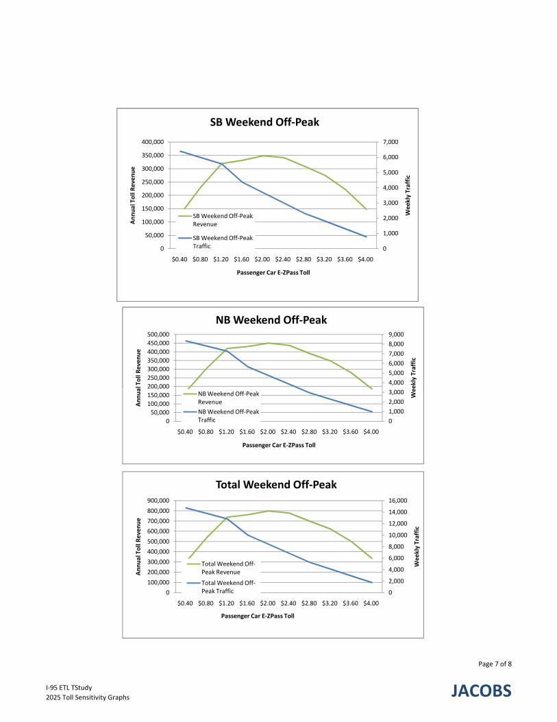
0
1,000
2,000
3,000
4,000
5,000
6,000
7,000
0
50,000
100,000
150,000
200,000
250,000
300,000
350,000
400,000
$0.40 $0.80 $1.20 $1.60 $2.00 $2.40 $2.80 $3.20 $3.60 $4.00
Weekly Traffic
Annual Toll Reven
ue
Passenger Car E‐ZPass Toll
SB Weekend Off‐Peak
SB Weekend Off‐Peak Revenue
SB Weekend Off‐Peak Traffic
4,000
5,000
6,000
7,000
8,000
9,000
200,000
250,000
300,000
350,000
400,000
450,000
500,000
ekly Traffic
l Toll Reven
ue
NB Weekend Off‐Peak
0
1,000
2,000
3,000
4,000
5,000
6,000
7,000
0
50,000
100,000
150,000
200,000
250,000
300,000
350,000
400,000
$0.40 $0.80 $1.20 $1.60 $2.00 $2.40 $2.80 $3.20 $3.60 $4.00
Weekly Traffic
Annual Toll Reven
ue
Passenger Car E‐ZPass Toll
SB Weekend Off‐Peak
SB Weekend Off‐Peak Revenue
SB Weekend Off‐Peak Traffic
0
1,000
2,000
3,000
4,000
5,000
6,000
7,000
8,000
9,000
0
50,000
100,000
150,000
200,000
250,000
300,000
350,000
400,000
450,000
500,000
$0.40 $0.80 $1.20 $1.60 $2.00 $2.40 $2.80 $3.20 $3.60 $4.00
Weekly Traffic
Annual Toll Reven
ue
Passenger Car E‐ZPass Toll
NB Weekend Off‐Peak
NB Weekend Off‐Peak Revenue
NB Weekend Off‐Peak Traffic
0
2,000
4,000
6,000
8,000
10,000
12,000
14,000
16,000
0
100,000
200,000
300,000
400,000
500,000
600,000
700,000
800,000
900,000
$0.40 $0.80 $1.20 $1.60 $2.00 $2.40 $2.80 $3.20 $3.60 $4.00
Weekly Traffic
Annual Toll Reven
ue
Passenger Car E‐ZPass Toll
Total Weekend Off‐Peak
Total Weekend Off‐Peak Revenue
Total Weekend Off‐Peak Traffic
I‐95 ETL TStudy
2025 Toll Sensitivity Graphs
Page 7 of 8
JACOBS
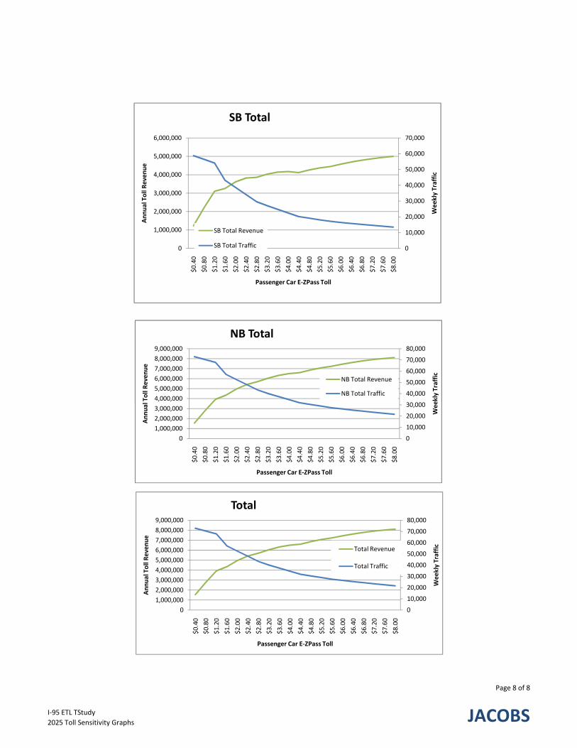
0
10,000
20,000
30,000
40,000
50,000
60,000
70,000
0
1,000,000
2,000,000
3,000,000
4,000,000
5,000,000
6,000,000
$0.40
$0.80
$1.20
$1.60
$2.00
$2.40
$2.80
$3.20
$3.60
$4.00
$4.40
$4.80
$5.20
$5.60
$6.00
$6.40
$6.80
$7.20
$7.60
$8.00
Weekly Traffic
Annual Toll Reven
ue
Passenger Car E‐ZPass Toll
SB Total
SB Total Revenue
SB Total Traffic
40,000
50,000
60,000
70,000
80,000
4,000,000
5,000,000
6,000,000
7,000,000
8,000,000
9,000,000
ekly Traffic
Toll Reven
ue
NB Total
NB Total Revenue
NB Total Traffic
0
10,000
20,000
30,000
40,000
50,000
60,000
70,000
0
1,000,000
2,000,000
3,000,000
4,000,000
5,000,000
6,000,000
$0.40
$0.80
$1.20
$1.60
$2.00
$2.40
$2.80
$3.20
$3.60
$4.00
$4.40
$4.80
$5.20
$5.60
$6.00
$6.40
$6.80
$7.20
$7.60
$8.00
Weekly Traffic
Annual Toll Reven
ue
Passenger Car E‐ZPass Toll
SB Total
SB Total Revenue
SB Total Traffic
0
10,000
20,000
30,000
40,000
50,000
60,000
70,000
80,000
0
1,000,000
2,000,000
3,000,000
4,000,000
5,000,000
6,000,000
7,000,000
8,000,000
9,000,000
$0.40
$0.80
$1.20
$1.60
$2.00
$2.40
$2.80
$3.20
$3.60
$4.00
$4.40
$4.80
$5.20
$5.60
$6.00
$6.40
$6.80
$7.20
$7.60
$8.00
Weekly Traffic
Annual Toll Reven
ue
Passenger Car E‐ZPass Toll
NB Total
NB Total Revenue
NB Total Traffic
0
10,000
20,000
30,000
40,000
50,000
60,000
70,000
80,000
0
1,000,000
2,000,000
3,000,000
4,000,000
5,000,000
6,000,000
7,000,000
8,000,000
9,000,000
$0.40
$0.80
$1.20
$1.60
$2.00
$2.40
$2.80
$3.20
$3.60
$4.00
$4.40
$4.80
$5.20
$5.60
$6.00
$6.40
$6.80
$7.20
$7.60
$8.00
Weekly Traffic
Annual Toll Reven
ue
Passenger Car E‐ZPass Toll
Total
Total Revenue
Total Traffic
I‐95 ETL TStudy
2025 Toll Sensitivity Graphs
Page 8 of 8
JACOBS

APPENDIX D
Acronyms/Abbreviations
List of Acronyms/Abbreviations
MDTA Maryland Transportation Authority
Jacobs Jacobs Engineering Group
ETL Express Toll Lanes
T&R Traffic and Toll Revenue
BMC Model Baltimore Metropolitan Council’s travel demand model
VISSIM Model VISSIM micro‐simulation model
T&R Model Toll Schedule and Toll Revenue Model
VOT Value of Time
JFK John F. Kennedy Memorial Highway
Hatem Thomas J. Hatem Memorial Bridge
FMT Fort McHenry Tunnel
BHT Baltimore Harbor Tunnel
FSK Francis Scott Key Bridge
Bay William Preston Lane Jr. Memorial Bay Bridge
Nice Governor Harry W. Nice Memorial Bridge
ICC/MD 200 Intercounty Connector
SR State Route
BRT Bus Rapid Transit
GDP Gross Domestic Product
NBER National Bureau of Economic Research
CBO Congressional Budget Office
FRB Federal Reserve Bank
IMF International Monetary Fund
IPI Industrial Production Index
VMT Vehicle Miles Traveled
EIA Energy Information Administration
WTI West Texas Intermediate Crude Oil Price
GTL Gas‐to‐Liquid
APTA American Public Transportation Association
PMT Passenger Miles Traveled
SIQSS Stanford Institute for the Quantitative Study of Society
GSP Gross State Product
MSAs Metropolitan Statistical Areas
GRP Gross Regional Product
BLS Bureau of Labor Statistics
ETC Electronic Toll Collection


![Welcome [mdta.maryland.gov]...May 14, 2019 · A Notice of Toll Due will be sent to the registered owner of the vehicle for the Video Toll due Due to higher processing costs, the](https://img.pdfslide.net/doc/110x75/5ea802ff1fca5c499c17e9a8/welcome-mdta-may-14-2019-a-notice-of-toll-due-will-be-sent-to-the-registered.jpg)