Phases of the ISM / Heidelberg 30th July 2013

Mass Distribution of the Molecular Phase of the ISM

Jouni Kainulainen (MPIA)

With: J. Alves, H. Beuther, C. Federrath, T. Henning, S. Ragan, J. C. Tan, A. Stutz

Jouni Kainulainen Phases of the ISM / Heidelberg 30th July 2013

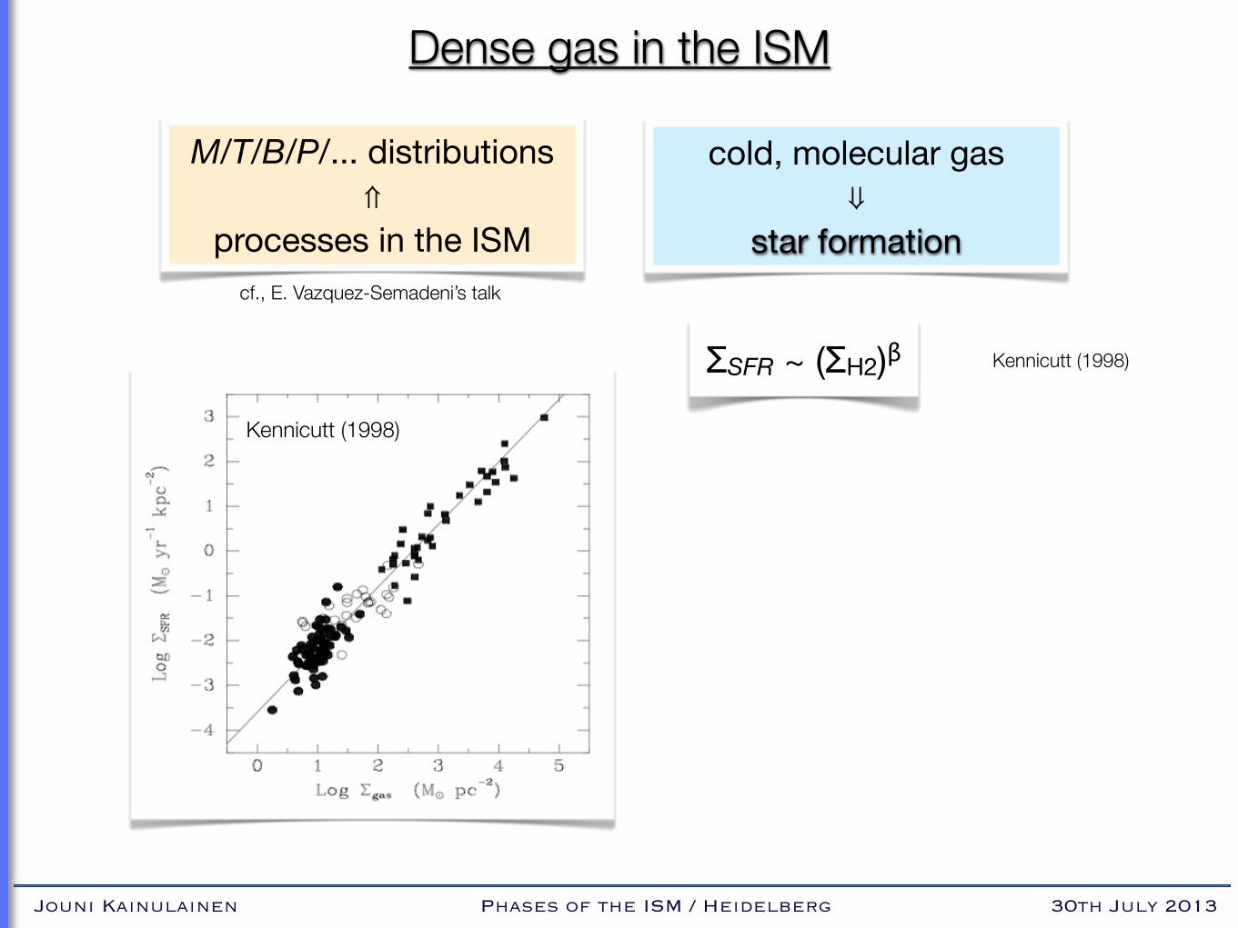
Dense gas in the ISM

M/T/B/P/... distributions⇑

processes in the ISMcf., E. Vazquez-Semadeni’s talk

Audit & Hennebelle (2005)

cold, molecular gas⇓

star formation

Jouni Kainulainen Phases of the ISM / Heidelberg 30th July 2013

Dense gas in the ISM

ΣSFR ~ (ΣH2)β Kennicutt (1998)

Kennicutt (1998)

M/T/B/P/... distributions⇑

processes in the ISMcf., E. Vazquez-Semadeni’s talk

cold, molecular gas⇓

star formation

Jouni Kainulainen Phases of the ISM / Heidelberg 30th July 2013

Lada et al. (2010)

ΣSFR ~ fdg(Σgas)β Lada et al. (2012)

This talk:

1. Observations: Quantifying dense gas fractions of MCs with dust extinction.

2. Theory: What parameters set how much dense gas molecular clouds have?

Dense gas in the ISM

ΣSFR ~ (ΣH2)β Kennicutt (1998)

M/T/B/P/... distributions⇑

processes in the ISMcf., E. Vazquez-Semadeni’s talk

cold, molecular gas⇓

star formation

Jouni Kainulainen Phases of the ISM / Heidelberg 30th July 2013

1. Observing the Mass Distribution of the ISM?

Column density

0.1 1 10 100 1000

N(H2) [x 1021 cm-2], or Av [mag]

HI →H2

~cold phase of the ISM

<N(H2)> low-M cores high-M cores

CO

Herschel/dust emission

NIR dust extinction

MIR dust extinction

Jouni Kainulainen Phases of the ISM / Heidelberg 30th July 2013

Near-IR Dust ExtinctionDobashi et al. (2010)

Kainulainen et al. (2009)

using 2MASS data

• NIR photometry of background stars.

• FWHM ~ 2’.

• N(H2) ~ 1-25 x 1021 cm-2.

Jouni Kainulainen Phases of the ISM / Heidelberg 30th July 2013

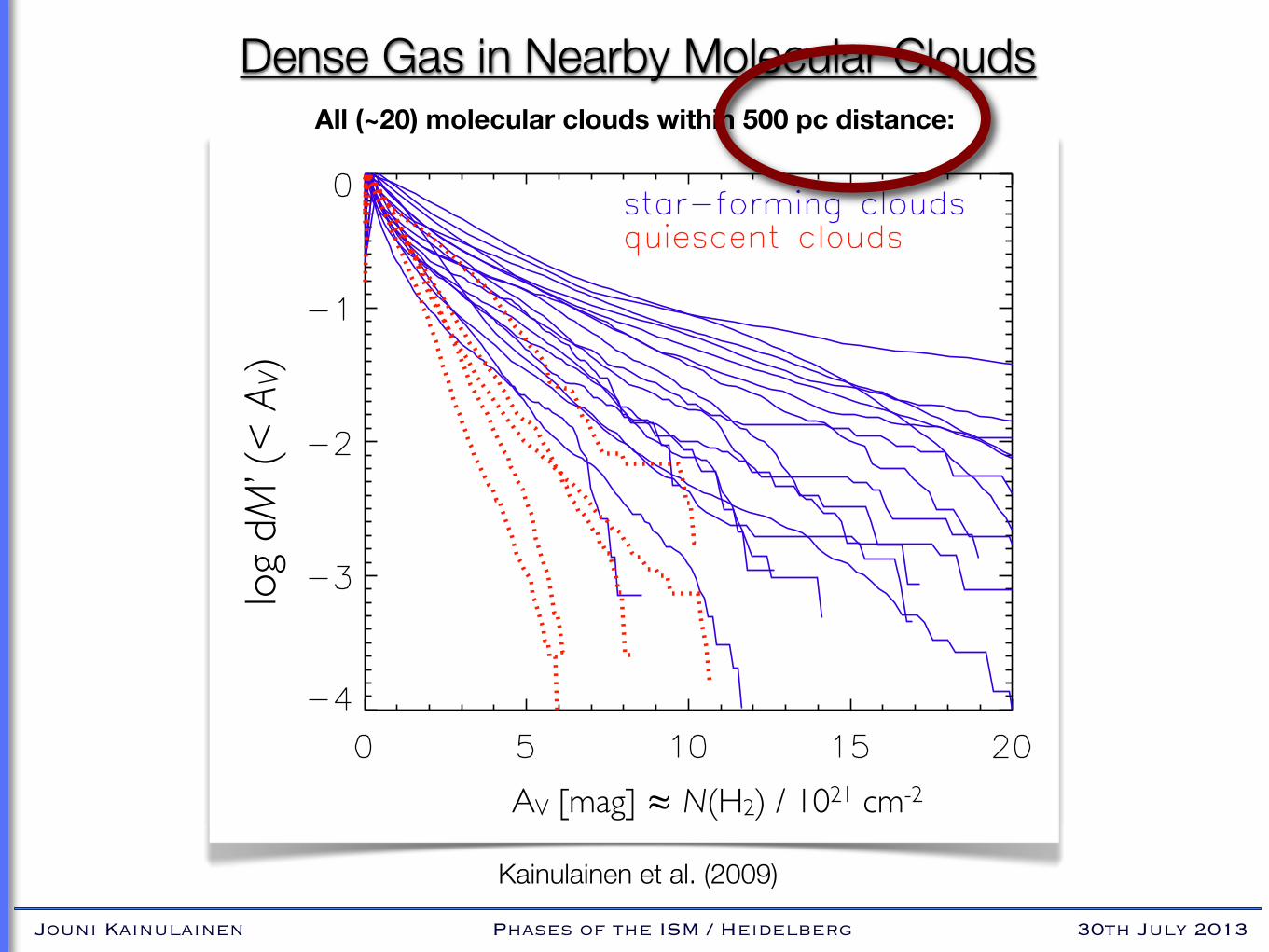
Dense Gas in Nearby Molecular Clouds

Kainulainen et al. (2009)

log

dM’ (

< AV)

AV [mag] ≈ N(H2) / 1021 cm-2

All (~20) molecular clouds within 500 pc distance:

Jouni Kainulainen Phases of the ISM / Heidelberg 30th July 2013

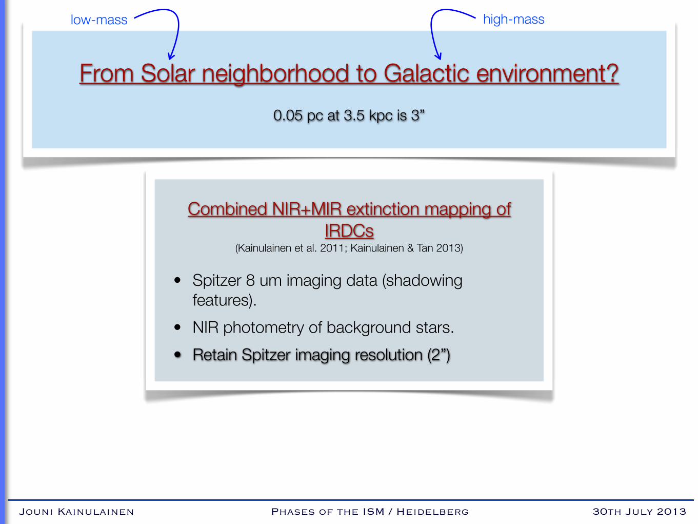
Combined NIR+MIR extinction mapping of IRDCs

(Kainulainen et al. 2011; Kainulainen & Tan 2013)

• Spitzer 8 um imaging data (shadowing features).

• NIR photometry of background stars.

• Retain Spitzer imaging resolution (2”)

From Solar neighborhood to Galactic environment?

0.05 pc at 3.5 kpc is 3”

low-mass high-mass

Jouni Kainulainen Phases of the ISM / Heidelberg 30th July 2013

Dust extinction map8 um + NIR photometry

Kainulainen et al. (2013)

Example: “The Snake”; D = 3.5 kpc

35’ ~ 35 pc at 3.5 kpc

FWHM = 2”N(H2) ~ 2 - 150 x 1021 cm-2

Jouni Kainulainen Phases of the ISM / Heidelberg 30th July 2013

Jouni Kainulainen Phases of the ISM / Heidelberg 30th July 2013

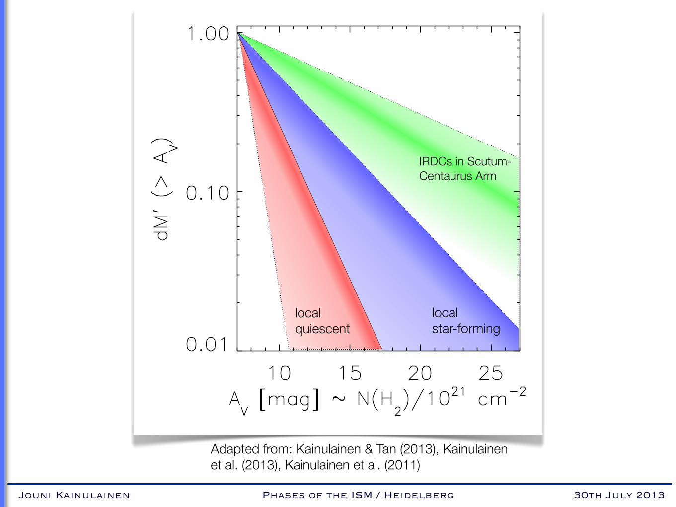
local star-forming

local quiescent

IRDCs in Scutum-Centaurus Arm

Adapted from: Kainulainen & Tan (2013), Kainulainen et al. (2013), Kainulainen et al. (2011)

Jouni Kainulainen Phases of the ISM / Heidelberg 30th July 2013

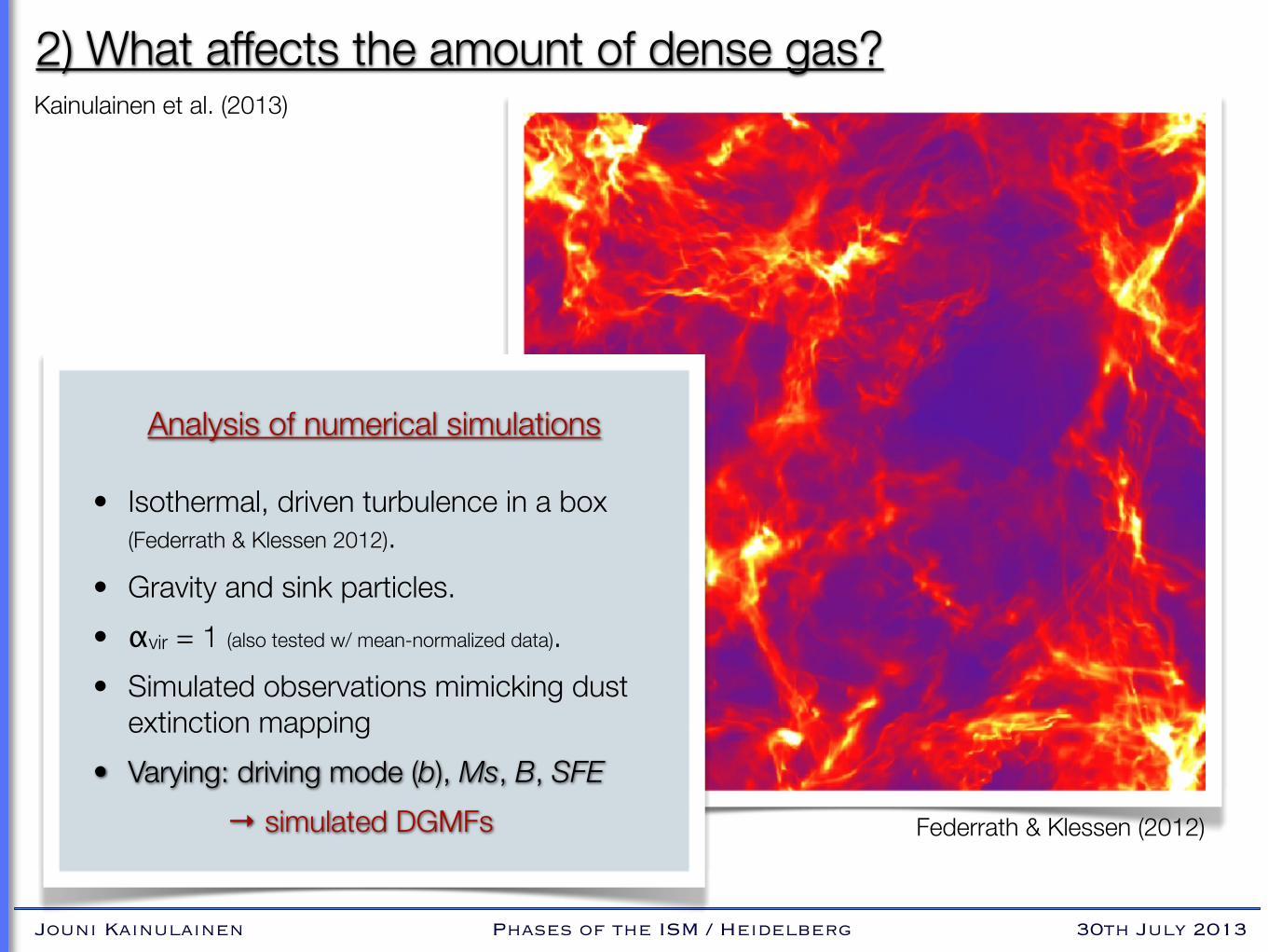
2) What affects the amount of dense gas?

Analysis of numerical simulations

• Isothermal, driven turbulence in a box (Federrath & Klessen 2012).

• Gravity and sink particles.

• αvir = 1 (also tested w/ mean-normalized data).

• Simulated observations mimicking dust extinction mapping

• Varying: driving mode (b), Ms, B, SFE

→ simulated DGMFs Federrath & Klessen (2012)

Kainulainen et al. (2013)

Jouni Kainulainen Phases of the ISM / Heidelberg 30th July 2013

2) What affects the amount of dense gas?

Analysis of numerical simulations

• Isothermal, driven turbulence in a box (Federrath & Klessen 2012).

• Gravity and sink particles.

• αvir = 1 (also tested w/ mean-normalized data).

• Simulated observations mimicking dust extinction mapping

• Varying: driving mode (b), Ms, B, SFE

→ simulated DGMFs Federrath & Klessen (2012)

Kainulainen et al. (2013)

Solenoidal forcing: b = 1/3 Compressive forcing: b = 1

Federrath – RSF2013 – Ringberg – 26/06/2013

Jouni Kainulainen Phases of the ISM / Heidelberg 30th July 2013

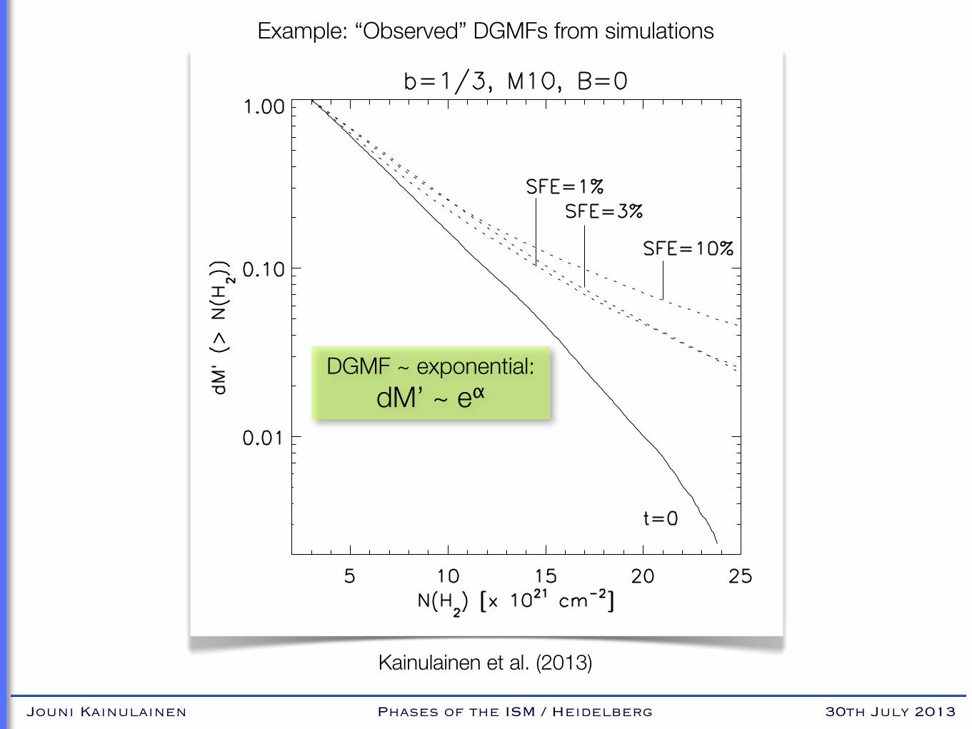
Kainulainen et al. (2013)

Example: “Observed” DGMFs from simulations

DGMF ~ exponential:dM’ ~ eα

Jouni Kainulainen Phases of the ISM / Heidelberg 30th July 2013

Kainulainen et al. (2013)

Nearby star-forming clouds

Nearby quiescent clouds

Massive IRDCs

Fully compressiveFully solenoidal

Exp

onen

tial s

lope

of t

he D

GM

F

Jouni Kainulainen Phases of the ISM / Heidelberg 30th July 2013

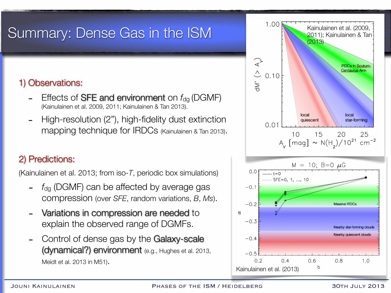
2) Predictions:(Kainulainen et al. 2013; from iso-T, periodic box simulations)

- fdg (DGMF) can be affected by average gas compression (over SFE, random variations, B, Ms).

- Variations in compression are needed to explain the observed range of DGMFs.

- Control of dense gas by the Galaxy-scale (dynamical?) environment (e.g., Hughes et al. 2013,

Meidt et al. 2013 in M51).

Summary: Dense Gas in the ISM

1) Observations:

- Effects of SFE and environment on fdg (DGMF) (Kainulainen et al. 2009, 2011; Kainulainen & Tan 2013).

- High-resolution (2”), high-fidelity dust extinction mapping technique for IRDCs (Kainulainen & Tan 2013).

Kainulainen et al. (2013)

Kainulainen et al. (2009, 2011); Kainulainen & Tan (2013)