Embed Size (px)
Citation preview

Mass Generation, the Cosmological Constant Problem,Conformal Symmetry, and the Higgs Boson
Philip D. MannheimDepartment of Physics, University of Connecticut, Storrs, CT 06269, USA
email: [email protected]
January 29, 2017
Abstract
In 2013 the Nobel Prize in Physics was awarded to Francois Englert and Peter Higgs for theirwork in 1964 along with the late Robert Brout on the mass generation mechanism (the Higgsmechanism) in local gauge theories. This mechanism requires the existence of a massive scalarparticle, the Higgs boson, and in 2012 the Higgs boson was finally discovered at the Large HadronCollider after being sought for almost half a century. In this article we review the work that ledto the discovery of the Higgs boson and discuss its implications. We approach the topic fromthe perspective of a dynamically generated Higgs boson that is a fermion-antifermion bound staterather than an elementary field that appears in an input Lagrangian. In particular, we emphasizethe connection with the Barden-Cooper-Schrieffer theory of superconductivity. We identify thedouble-well Higgs potential not as a fundamental potential but as a mean-field effective Lagrangianwith a dynamical Higgs boson being generated through a residual interaction that accompanies themean-field Lagrangian. We discuss what we believe to be the key challenge raised by the discoveryof the Higgs boson, namely determining whether it is elementary or composite, and through study ofa conformal invariant field theory model as realized with critical scaling and anomalous dimensions,suggest that the width of the Higgs boson might serve as a suitable diagnostic for discriminatingbetween an elementary Higgs boson and a composite one. We discuss the implications of Higgsboson mass generation for the cosmological constant problem, as the cosmological constant receivescontributions from the very mechanism that generates the Higgs boson mass in the first place.We show that the contribution to the cosmological constant due to a composite Higgs boson ismore tractable and under control than the contribution due to an elementary Higgs boson, and ispotentially completely under control if there is an underlying conformal symmetry not just in acritical scaling matter sector (which there would have to be if all mass scales are to be dynamical),but equally in the gravity sector to which the matter sector couples.
1
arX
iv:1
610.
0890
7v2
[he
p-ph
] 3
0 Ja
n 20
17
Contents
1 Introduction 4
1.1 Preamble . . . . . . . . . . . . . . . . . . . . . . . . . . . . . . . . . . . . . . . . . . . 4
1.2 Ideas About Mass and Implications for the Cosmological Constant Problem . . . . . . . 5
2 The Higgs Boson Discovery 5
3 Background Leading to the Higgs Mechanism and Higgs Boson Papers in 1964 6
4 Broken Symmetry 7
4.1 Global Discrete Symmetry – Real Scalar Field – Goldstone (1961) . . . . . . . . . . . . 7
4.2 Global Continuous Symmetry – Complex Scalar Field – Goldstone (1961) . . . . . . . . 8
4.3 Local Continuous Symmetry – Complex Scalar Field and Gauge Field – Higgs (1964) . 10
5 The Physics Behind Broken Symmetry 10
5.1 The Effective Action . . . . . . . . . . . . . . . . . . . . . . . . . . . . . . . . . . . . . 10
5.2 The Nature of Broken Symmetry . . . . . . . . . . . . . . . . . . . . . . . . . . . . . . 12
5.3 Broken Symmetry and Multiplevaluedness . . . . . . . . . . . . . . . . . . . . . . . . . 13
5.4 Cooper Pairing in Superconductivity . . . . . . . . . . . . . . . . . . . . . . . . . . . . 15
5.5 Degenerate Fermion Vacua . . . . . . . . . . . . . . . . . . . . . . . . . . . . . . . . . . 17
5.6 Symmetry Breaking by Fermion Bilinear Composites . . . . . . . . . . . . . . . . . . . 19
6 Is the Higgs Boson Elementary or Composite? 21
6.1 What Exactly is the Higgs Field? . . . . . . . . . . . . . . . . . . . . . . . . . . . . . . 21
6.2 Nambu-Jona-Lasinio Chiral Model as a Mean-Field Theory . . . . . . . . . . . . . . . . 22
6.3 The Collective Scalar and Pseudoscalar Tachyon Modes . . . . . . . . . . . . . . . . . . 25
6.4 The Collective Goldstone and Higgs Modes . . . . . . . . . . . . . . . . . . . . . . . . . 26
7 The Abelian Gluon Model 27
7.1 The Schwinger-Dyson Equation . . . . . . . . . . . . . . . . . . . . . . . . . . . . . . . 27
7.2 Renormalization Group Analysis . . . . . . . . . . . . . . . . . . . . . . . . . . . . . . . 30
7.3 Johnson-Baker-Willey Electrodynamics . . . . . . . . . . . . . . . . . . . . . . . . . . . 31
7.4 The Baker-Johnson Evasion of the Goldstone Theorem . . . . . . . . . . . . . . . . . . 32
7.5 The Shortcomings of the Quenched Ladder Approximation . . . . . . . . . . . . . . . . 33
8 Structure of Johnson-Baker-Willey Electrodynamics 36
8.1 JBW Electrodynamics as a Mean-Field Theory . . . . . . . . . . . . . . . . . . . . . . 36
8.2 Vacuum Structure of JBW Electrodynamics at γθ(α) = −1. . . . . . . . . . . . . . . . . 40
8.3 Dynamical Tachyons of m = 0 Electrodynamics at γθ(α) = −1 . . . . . . . . . . . . . . 42
8.4 Dynamical Goldstone Boson of m 6= 0 Electrodynamics at γθ(α) = −1 . . . . . . . . . . 42
8.5 Dynamical Higgs Boson of m 6= 0 Electrodynamics at γθ(α) = −1 . . . . . . . . . . . . 43
8.6 Some Other Approaches . . . . . . . . . . . . . . . . . . . . . . . . . . . . . . . . . . . 46
8.7 Weak Coupling Versus Strong Coupling . . . . . . . . . . . . . . . . . . . . . . . . . . . 49
8.8 Anomalous Dimensions and the Renormalizability of the Four-Fermion Interaction . . . 49
9 Why Does an Elementary Higgs Model Work so Well in Weak Interactions if theHiggs Boson is Dynamical? 52
2
10 Mass Generation and the Cosmological Constant Problem 5410.1 From a Dynamical Higgs Boson to Conformal Gravity . . . . . . . . . . . . . . . . . . . 5410.2 The Vacuum Energy Density Problem . . . . . . . . . . . . . . . . . . . . . . . . . . . 5510.3 Is the Standard Gravity Cosmological Constant Problem Properly Posed? . . . . . . . . 5910.4 The Consistency of Quantum Conformal Gravity . . . . . . . . . . . . . . . . . . . . . 6110.5 The Conformal Gravity Cancellation of Infinities . . . . . . . . . . . . . . . . . . . . . . 64
11 Some Other Aspects of Conformal Symmetry and Conformal Gravity 6811.1 Conformal gravity and the Dark Matter Problem . . . . . . . . . . . . . . . . . . . . . 6811.2 Conformal Invariance and the Metrication of Electromagnetism . . . . . . . . . . . . . 7311.3 Conformal Gravity and the Metrication of the Fundamental Forces . . . . . . . . . . . 7411.4 The Inevitability of Conformal Gravity . . . . . . . . . . . . . . . . . . . . . . . . . . . 7511.5 A Theory of Everything . . . . . . . . . . . . . . . . . . . . . . . . . . . . . . . . . . . 77
12 Comparing Conformal Symmetry and Supersymmetry 78
13 Summary 79
14 The Moral of the Story 79
15 Acknowledgments 80
3
1 Introduction
1.1 Preamble
The 2013 Nobel Prize in Physics was awarded to Francois Englert and Peter Higgs for their work in 1964on the Higgs mechanism, work that led in 2012 to the discovery at the CERN Large Hadron Collider(LHC) of the Higgs Boson after its being sought for almost 50 years. It is great tragedy that RobertBrout, the joint author with Francois Englert of one of the papers that led to the 2013 Nobel Prize,died in 2011, just one year before the discovery of the Higgs boson and two years before the awardingof the Nobel prize for it. (For me personally this is keenly felt since my first post-doc was with Robertand Francois in Brussels 1970 - 1972.)
The paper coauthored by Englert and Brout appeared on August 31, 1964 in Physical ReviewLetters [1] after being submitted on June 26, 1964 and was two and one half pages long. Higgs wrotetwo papers on the topic. His first paper appeared on September 15, 1964 in Physics Letters [2] afterbeing submitted on July 27, 1964 and was one and one half pages long, and the second paper appearedon October 19, 1964 in Physical Review Letters [3] after being submitted on August 31, 1964 and wasalso one and one half pages long. Thus a grand total of just five and one half pages.
The significance of the Higgs mechanism introduced in these papers and the Higgs Boson identifiedby Higgs is that they are tied in with the theory of the origin of mass, and of the way that mass canarise through collective effects (known as broken symmetry) that only occur in systems with a largenumber of degrees of freedom. Such collective effects are properties that a system of many objectscollectively possess that each one individually does not – the whole being greater than the sum of itsparts. A typical example is temperature. A single molecule of H2O does not have a temperature, andone cannot tell if it was taken from ice, water or steam. These different phases are collective propertiesof large numbers of H2O molecules acting in unison. Moreover, as one changes the temperature all theH2O molecules can act collectively to change the phase (freezing water into ice for instance), with itbeing the existence of such phase changes that is central to broken symmetry.
I counted at least 21 times that Nobel Prizes in Physics have in one way or another been givenfor aspects of the problem: Dirac (1933); Anderson (1936); Lamb (1955); Landau (1962); Tomon-aga, Schwinger, Feynman (1965); Gell-Mann (1969); Bardeen, Cooper, Schrieffer (1972); Richter,Ting (1976); Glashow, Salam, Weinberg (1979); Wilson (1982); Rubbia, van der Meer (1984); Fried-man, Kendall, Taylor (1990); Lee, Osheroff, Richardson (1996); ’t Hooft,Veltman (1999); Abrikosov,Ginzburg, Leggett (2003); Gross, Politzer, Wilczek (2004); Mather, Smoot (2006); Nambu, Kobayashi,Maskawa (2008); Perlmutter, Schmidt, Reiss (2011); Englert, Higgs (2013); Kajita, McDonald (2015).And this leaves out Anderson who made major contributions to collective aspects of mass generationand Yang who (with Mills) developed non-Abelian Yang-Mills gauge theories but got Nobel prizes (An-derson 1977, Yang 1957) for something else. While the Nobel prizes to Mather and Smoot and toPerlmutter, Schmidt, and Reiss were for cosmological discoveries (cosmic anisotropy and cosmic accel-eration), because they tie in with the cosmological constant problem, a problem which itself ties in withmass generation and the Higgs mechanism, I have included them in the list. Since in the absence ofany mass scales one has an underlying conformal symmetry, the interplay of mass generation with thecosmological constant problem, with this underlying conformal symmetry, and with its local conformalgravity extension will play a central role in this article, as I review the work and ideas that led up tothe discovery of the Higgs boson and then discuss its implications.
4

1.2 Ideas About Mass and Implications for the Cosmological ConstantProblem
As introduced by Newton mass was mechanical. The first ideas on dynamical mass were due to Poincare(Poincare stresses needed to stabilize an electron all of whose mass came from its own electromagneticself-energy according to mc2 = e2/r). However this was all classical.
With quantum field theory, the mass of a particle is able to change through self interactions (radia-tive corrections to the self-energy – Lamb shift) to give m = m0 + δm, or through a change in vacuum(Bardeen, Cooper, Schrieffer – BCS theory) according to E = p2/2m−∆ where ∆ is the self-consistentgap parameter. Then through Nambu (1960) and Goldstone (1961) the possibility arose that not justsome but in fact all of the mass could come from self interaction, and especially so for gauge bosons,viz. Anderson (1958, 1963), Englert and Brout (1964), Higgs (1964), Guralnik, Hagen, and Kibble(1964). This culminated in the Weinberg (1967), Salam (1968), and Glashow (1961, 1970) renormaliz-able SU(2)×U(1) local gauge theory of electroweak interactions, and the confirming discoveries first ofweak neutral currents (1973), then charmed particles (1974), then the intermediate vector bosons of theweak interactions (1983), and finally the Higgs boson (2012). All of this is possible because of Dirac’sHilbert space formulation of quantum mechanics in which one sets ψ(x) = 〈x|ψ〉, with the physics beingin the properties of the states |ψ〉. We thus live in Hilbert space and not in coordinate space, and notonly that, there is altogether more in Hilbert space than one could imagine, such as half-integer spinand collective macroscopic quantum systems such as superconductors and superfluids. In this Hilbertspace we find an infinite Dirac sea of negative energy particles. Because of their large number thesedegrees of freedom can collectively act to provide the dynamics needed to produce mass generation andthe Higgs boson. Since the dynamical generation of mass leads to contributions to the cosmologicalconstant (i.e. to the energy density of the vacuum), mass generation and the cosmological constantproblem are intimately connected. Moreover, since gravity couples to energy density and not just toenergy density difference, gravity knows where the zero of energy is, to thus be sensitive to the massgeneration mechanism. Gravity and the mass generation mechanism are thus intimately connected toeach other.
2 The Higgs Boson Discovery
The discovery of the Higgs boson was announced by CERN on July 4, 2012, accompanied by simulta-neous announcements by the experimental groups ATLAS and CMS at the Large Hadron Collider atCERN, as then followed by parallel publications that were simultaneously submitted to Physics LettersB on July 31, 2012 and published on September 17, 2012, one publication by the ATLAS Collaboration[4], and the other by the CMS Collaboration [5]. The ATLAS paper had 2924 authors, and the CMSpaper had 2883. The Higgs boson signature used by both collaborations was to look for the lepton pairsthat would be found in the decay products of any Higgs boson that might be produced in high energyproton proton collisions at the Large Hadron Collider.
From amongst a set of 1015 proton-proton collisions produced at the Large Hadron Collider, of theorder of 240,000 collisions produce a Higgs boson. Of them just 350 decay into pairs of gamma rays,and of those gamma rays just 8 decay into a pair of leptons. The search for the Higgs boson is thus asearch for some very rare events. Thus to see Higgs bosons one needs an energy high enough to producethem and the sensitivity to see such rare decays when they are produced. In searches over the yearsit was not known in what energy regime to look for Higgs particles, with the Large Hadron Colliderproving to be the collider whose energy was high enough that one could finally explore in detail the 125GeV energy domain where the Higgs boson was ultimately found to exist.
5

3 Background Leading to the Higgs Mechanism and Higgs
Boson Papers in 1964
In order to characterize macroscopic ordered phases in a general way Landau introduced the conceptof a macroscopic order parameter φ. For a ferromagnet for instance φ would represent the spontaneousmagnetization M and would be a matrix element of a field operator φ in an ordered quantum statethat described the ordered magnetic phase. Building on this approach Ginzburg and Landau [6] wrote
down a Lagrangian for such a φ for a superconductor, with kinetic energy ~∇φ · ~∇φ/2 and potentialV (φ) = λφ4/4 +m2(1−TC/T )φ2/2, where TC is the critical temperature, and m is a real constant. Fortemperatures above the critical temperature the potential would have the shape of a single well, viz.like the letter U, with the coefficient of the φ2 term being positive, and with the potential minimumbeing at φ = 0. For temperatures below the critical temperature the potential would have the shapeof a double well, viz. like the letter W, with the coefficient of the φ2 term being negative, and withthe potential minimum being at φ = m(TC/T − 1)1/2/λ1/2. Above the critical temperature the orderparameter would be zero at the minimum of the potential (normal phase with state vector |N〉 in which〈N |φ|N〉 = 0). Below the critical temperature the order parameter would be nonzero (superconductingstate |S〉 in which φ = 〈S|φ|S〉 = m(TC/T − 1)1/2/λ1/2 is nonzero).
In 1957 Bardeen, Cooper, and Schrieffer [7] developed a microscopic theory of superconductivity(BCS) based on Cooper pairing of electrons in the presence of a filled Fermi sea of electrons, andexplicitly constructed the state |S〉. In this state the matrix element 〈S|ψ(x)ψ(x)|S〉 was equal to aspacetime-independent function ∆, the gap parameter, which led to a mass shift to electrons propagatingin a superconductor of the form E = p2/2m−∆. The gap parameter ∆ would be temperature dependent(∼ (TC − T )1/2), and would only be nonzero below the critical temperature. In 1959 Gorkov [8] wasable to derive the Ginzburg-Landau Lagrangian starting from the BCS theory and identify the orderparameter as the spacetime-dependent φ(x) = 〈C|ψ(x)ψ(x)|C〉 where |C〉 is a coherent state in theHilbert space based on |S〉. In the superconducting case then φ is not itself a quantum-field-theoreticoperator (viz. a q-number operator that would have a canonical conjugate with which it would notcommute) but is instead a c-number matrix element of a q-number field operator ψψ in a macroscopiccoherent quantum state.
In 1958 Anderson [9] used the BCS theory to explain the Meissner effect, an effect in which elec-tromagnetism becomes short range inside a superconductor, with photons propagating in it becomingmassive. The effect was one of spontaneous breakdown of local gauge invariance, and was explored indetail by Anderson [9] and Nambu [10].
In parallel with these studies Nambu [11], Goldstone [12], and Nambu and Jona-Lasinio [13] exploredthe spontaneous breakdown of some continuous global symmetries and showed that collective masslessexcitations (Goldstone bosons) were generated, and that the analog gap parameter would provide fordynamically induced fermion masses. In 1962 Goldstone, Salam, and Weinberg [14] showed that therewould always be massless Goldstone bosons in any Lorentz invariant theory in which a continuousglobal symmetry was spontaneously broken. While one could avoid this outcome if the symmetry wasalso broken in the Lagrangian, as was, through the weak interaction, thought to be the case for thepion, a non-massless but near Goldstone particle (i.e. one with broken symmetry suppressed couplingsto matter at low energies), in general the possible presence of massless Goldstone bosons was a quiteproblematic outcome because it would imply the existence of non-observed long range forces.
In 1962 Schwinger [15, 16] raised the question of whether gauge invariance actually required thatphotons be massless, and noted for the photon propagator D(q2) = 1/[q2− q2Π(q2)] that if the vacuumpolarization Π(q2) had a massless pole of the form Π(q2) = m2/q2, D(q2) would behave as the massiveparticle D(q2) = 1/[q2 −m2]. A massless Goldstone boson could thus produce a massive vector boson.
With Anderson having shown that a photon would become massive in a superconductor, there was
6
a spirited discussion in the literature (Anderson [17], Klein and Lee [18], Gilbert [19]) as to whetheran effect such as this might hold in a relativistic theory as well or whether it might just have beenan artifact of the fact that the BCS theory was non-relativistic. With the work of Englert and Brout[1] and Higgs [2, 3], and then Guralnik, Hagen, and Kibble [20], the issue was finally resolved, with itbeing established that in the relativistic case the Goldstone theorem did not in fact hold if there wasa spontaneous breakdown of a continuous local theory, with the would-be Goldstone boson no longerbeing an observable massless particle but instead combining with the initially massless vector bosonto produce a massive vector boson. Technically, this mechanism should be known as the Anderson,Englert, Brout, Higgs, Guralnik, Hagen, Kibble mechanism, and while it has undergone many namevariations over time, it is now commonly called the Higgs mechanism. What set Higgs’ work apart fromthe others was that in his 1964 Physical Review Letters paper Higgs noted that as well as a massivegauge boson there should also be an observable massive scalar boson, this being the Higgs boson.
At the time of its development in 1964 there was not much interest in the Higgs mechanism, with allof the Englert and Brout, Higgs, and Guralnik, Hagen and Kibble papers getting hardly any citationsduring the 1960s at all. The primary reason for this was that at the time there was little interestin non-Abelian Yang-Mills gauge theories in general, broken or unbroken, and not only was there noexperimental indication at all that one should consider them, it was not clear if Yang-Mills theorieswere even quantum-mechanically viable. All this changed in the early 1970s when ’t Hooft and Veltmanshowed that these theories were renormalizable, and large amounts of data started to point in thedirection of the relevance of non-Abelian gauge theories to physics, leading to the SU(3)×SU(2)×U(1)picture of strong, electromagnetic and weak interactions, which culminated in the discoveries of theW+, W− and Z0 intermediate vector bosons (1983) with masses that were generated by the Higgsmechanism, and then finally the Higgs boson itself (2012). What gave the Higgs boson the prominencethat it ultimately came to have was the realization that in the electroweak SU(2) × U(1) theory theHiggs boson not only gives masses to the gauge bosons while maintaining renormalizability, but throughits Yukawa couplings to the quarks and leptons of the theory it gives masses to the fermions as well.The Higgs boson is thus responsible not just for the masses of the gauge bosons then but for the massesof all the other fundamental particles as well, causing it to be dubbed the “god particle”.1
4 Broken Symmetry
4.1 Global Discrete Symmetry – Real Scalar Field – Goldstone (1961)
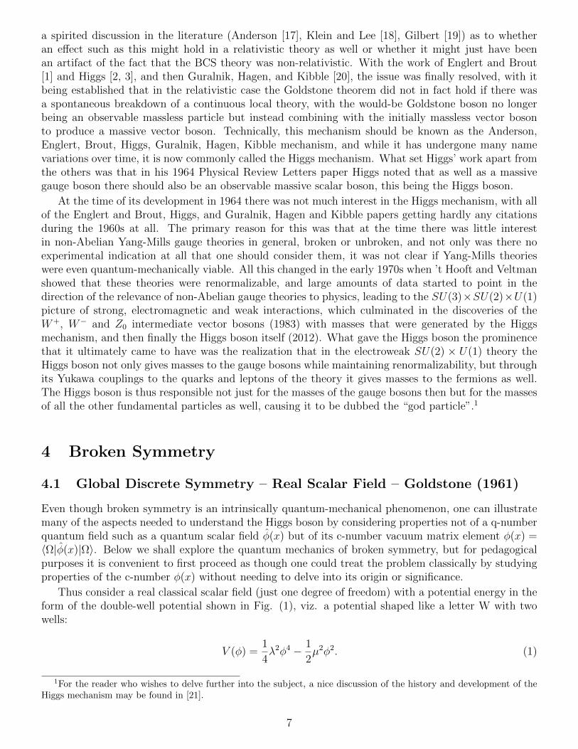
Even though broken symmetry is an intrinsically quantum-mechanical phenomenon, one can illustratemany of the aspects needed to understand the Higgs boson by considering properties not of a q-numberquantum field such as a quantum scalar field φ(x) but of its c-number vacuum matrix element φ(x) =〈Ω|φ(x)|Ω〉. Below we shall explore the quantum mechanics of broken symmetry, but for pedagogicalpurposes it is convenient to first proceed as though one could treat the problem classically by studyingproperties of the c-number φ(x) without needing to delve into its origin or significance.
Thus consider a real classical scalar field (just one degree of freedom) with a potential energy in theform of the double-well potential shown in Fig. (1), viz. a potential shaped like a letter W with twowells:
V (φ) =1
4λ2φ4 − 1
2µ2φ2. (1)
1For the reader who wishes to delve further into the subject, a nice discussion of the history and development of theHiggs mechanism may be found in [21].
7

Figure 1: Discrete Double Well Potential – V (φ) plotted as a function of φ.
This potential has a discrete symmetry under φ→ −φ, with its first two derivatives being given by
dV (φ)
dφ= λ2φ3 − µ2φ,
d2V (φ)
dφ2= 3λ2φ2 − µ2. (2)
The potential has a local maximum at φ = 0 where V (φ = 0) is zero and d2V (φ = 0)/dφ2 = −µ2 isnegative, and two-fold degenerate global minima at φ = +µ/λ and φ = −µ/λ where V (φ = ±µ/λ) isequal to −µ4/4λ2 and d2V (φ = ±µ/λ)/dφ2 = 2µ2 is positive. Since φ = 0 is a local maximum, if weconsider small oscillations around φ = 0 of the form φ = 0 + χ we generate a negative quadratic term−(1/2)µ2χ2 and a thus negative squared mass, viz. m2 = −µ2, a so-called tachyon. The tachyon signalsan instability of the configuration with φ = 0 (i.e. we roll away from the top of the hill).
However if we fluctuate around either global minimum (i.e. we oscillate in the vertical around eitherof the two valleys) by setting φ = ±µ/λ+ χ we get
V (φ) = − µ4
4λ2+ µ2χ2 ± µλχ3 +
1
4λ2χ4. (3)
The field χ now has the positive squared mass m2 = d2V (φ = ±µ/λ)/dφ2 = 2µ2 (= −2×m2(tachyon)).Thus (Goldstone [12]) the would-be tachyonic particle becomes a massive particle, and with one scalarfield we obtain one particle. This particle is the Higgs boson in embryo.
The −µ4/4λ2 potential term contributes to the cosmological constant, and would be unacceptablylarge (1060 times too large) if the boson has the 125 GeV mass that the Higgs boson has now beenfound to have.
All this arises because the minimum is two-fold degenerate, and picking either one breaks thesymmetry spontaneously, since while one could just as equally be in either one minimum or the other,one could not be in both. This is just like people at a dinner. Each one can take the cup to their left ortheir right, but once one person has done so, the rest have no choice. However, a person at the oppositeend of the table may not know what choice was made at the other end of the table and may make theopposite choice of cup, and thus persons in the middle could finish up with no cup. To ensure that thisdoes not happen we need long range correlations – hence massless Goldstone bosons.
4.2 Global Continuous Symmetry – Complex Scalar Field – Goldstone(1961)
Consider a complex scalar field (two degrees of freedom) φ = φ1 + iφ2 = reiθ, φ∗φ = φ21 + φ2
2 = r2, witha potential energy in the shape of a rotated letter W or a broad-brimmed, high-crowned Mexican Hatas exhibited in Fig. (2), viz.
8

Figure 2: Continuous Double Well Mexican Hat Potential – V (φ) plotted as a function of φ.
V (φ) =1
4λ2(φ∗φ)2 − 1
2µ2φ∗φ =
1
4λ2(φ2
1 + φ22)2 − 1
2µ2(φ2
1 + φ22). (4)
The potential has a continuous global symmetry of the form φ→ eiαφ with constant α, with derivatives
dV (φ)
dφ1
= λ2φ31 + λ2φ1φ
22 − µ2φ1,
dV (φ)
dφ2
= λ2φ32 + λ2φ2
1φ2 − µ2φ2. (5)
This potential has a local maximum at φ1 = 0, φ2 = 0 where V (φ = 0) is zero, and infinitely degenerateglobal minima at φ2
1 + φ22 = µ2/λ2 (the entire 360 degree valley or trough between the brim and the
crown of the Mexican hat). Again we would have a tachyon if we expand around the local maximum,only this time we would get two. However, if we fluctuate around any one of the global minima bysetting φ1 = µ/λ+ χ1, φ2 = χ2, we get
V (φ) = − µ4
4λ2+ µ2χ2
1 + µλχ31 +
1
4λ2χ4
1 + µλχ1χ22 +
λ2
2χ2
1χ22. (6)
The (embryonic) Higgs boson field is now χ1 with m2 = +2µ2. However, the field χ2 no has no mass atall [12] (it corresponds to horizontal oscillations along the valley floor), and is called a Goldstone bosonor, because of Nambu’s related work, a Nambu-Goldstone boson. Thus from a complex scalar field weobtain two particles. Since the Goldstone boson is massless, it travels at the speed of light. It is thusintrinsically relativistic, and being massless can provide for long range correlations. Moreover, if suchparticles exist then they could generate fermion masses entirely dynamically (Nambu [11], and Nambuand Jona-Lasinio [13]), with the pion actually serving this purpose.
The −µ4/4λ2 potential term remains and the cosmological constant problem is just as severe asbefore.
Now if we have massless particles, we would get long range forces (just like photons), and yet nuclearand weak forces are short range. So what can we do about such Goldstone bosons. Two possibilities -they could get some mass because the symmetry is not exact (pion mass), or we could get rid of themaltogether (the Higgs mechanism).
9

4.3 Local Continuous Symmetry – Complex Scalar Field and Gauge Field– Higgs (1964)
Consider the model studied by Higgs [3] consisting of a complex scalar field (two degrees of freedom)coupled to a massless vector gauge boson (another two degrees of freedom) for a total of four degreesof freedom in all, viz. φ = reiθ, φ∗φ = r2, Fµν = ∂µAν − ∂νAµ. The system has kinetic energy K andpotential energy V (φ):
K =1
2(−i∂µ + eAµ)(re−iθ)(i∂µ + eAµ)(reiθ)− 1
4FµνF
µν
=1
2∂µr∂
µr +1
2r2(eAµ − ∂µθ)(eAµ − ∂µθ)−
1
4FµνF
µν ,
V (φ) =1
4λ2(φ∗φ)2 − 1
2µ2φ∗φ =
1
4λ2r4 − 1
2µ2r2, (7)
and because of the gauge boson the system is now invariant under continuous local gauge transformationsof the form φ→ eiα(x)φ, eAµ → eAµ + ∂µα(x) with spacetime dependent α(x). With derivatives
dV (φ)
dr= λ2r3 − µ2r,
d2V (φ)
dr2= 3λ2r2 − µ2, (8)
the potential has a local maximum at r = 0 where V (r = 0) is zero and degenerate global minima atr = µ/λ (infinitely degenerate since independent of θ). Again we would have two tachyons if we expandaround the local maximum. So fluctuate around the global minimum by setting r = µ/λ+χ1, θ2 = χ2.On defining Bµ = Aµ − (1/e)∂µχ2 we obtain
K =1
2∂µχ1∂
µχ1 +e2µ2
2λ2BµB
µ − 1
4(∂µBν − ∂νBµ)(∂µBν − ∂νBµ) +
e2
2
(2µ
λχ1 + χ2
1
)BµB
µ,
V (φ) = − µ4
4λ2+ µ2χ2
1 + µλχ31 +
1
4λ2χ4
1. (9)
There is again a Higgs boson field χ1 with m2 = +2µ2. However, the field χ2 has disappeared completely.Instead the vector boson now has a nonzero mass given by m = eµ/λ. Since a massive gauge boson hasthree degrees of freedom (two transverse and one longitudinal) while a massless gauge boson such as thephoton only has two transverse degrees of freedom, the would-be massless Goldstone boson is absorbedinto the now massive gauge boson to provide its needed longitudinal degree of freedom. Hence a masslessGoldstone boson and a massless gauge boson are replaced by one massive gauge boson, with two long-range interactions being replaced by one short range interaction. This is known as the Higgs mechanismthough it was initially found by Anderson [9] in his study of the Meissner effect in superconductivity.The remaining fourth of the original four degrees of freedom becomes the massive Higgs boson, andits presence is an indicator that the Higgs mechanism has taken place. However, with the presence of−µ4/4λ2 term in V (φ), the cosmological constant problem remains as severe as before.
5 The Physics Behind Broken Symmetry
5.1 The Effective Action
To discuss broken symmetry in quantum field theory it is convenient to introduce local sources. Inthe Gell-Mann-Low adiabatic switching procedure one introduces a quantum-mechanical Lagrangiandensity L0 of interest, switches on a real local c-number source J(x) for some Hermitian quantum fieldφ(x) at time t = −∞, and switches J(x) off at t = +∞. While the source is active the Lagrangian
10
density of the theory is given by LJ = L0 + J(x)φ(x). Before the source is switched on the system isin the ground state |Ω−0 〉 of the Hamiltonian H0 associated with L0, and after the source is switchedoff the system is in the state |Ω+
0 〉. While |Ω−0 〉 and |Ω+0 〉 are both eigenstates of H0, they differ by a
phase, a phase that is fixed by J(x) according to
〈Ω+0 |Ω−0 〉|J = 〈ΩJ |T exp
[i∫d4x(L0 + J(x)φ(x))
]|ΩJ〉 = eiW (J), (10)
with this expression serving to define the functional W (J). As introduced, W (J) serves as the generatorof the connected J = 0 theory Green’s functions Gn
0 (x1, ..., xn) = 〈Ω0|T [φ(x1)...φ(xn)]|Ω0〉 according to
W (J) =∑n
1
n!
∫d4x1...d
4xnGn0 (x1, ..., xn)J(x1)...J(xn). (11)
On Fourier transforming the Green’s functions, we can expand W (J) about the point where all momentavanish, to obtain
W (J) =∑n
1
n!
∫d4x1...d
4xn
∫d4p1...d
4pnJ(x1)...J(xn)eip1·x1 ...eipn·xn(2π)4δ4(∑
pi)
×[Gn
0 (pi = 0) +∑
pipj∂
∂pi
∂
∂pjGn
0 (pk)|pk=0 + ...]
=∫d4x
[−ε(J) +
1
2Z(J)∂µJ∂
µJ + ....], (12)
with the first two terms in the last expression for W (J) being in the standard −V + K form requiredfor actions. With HJ being the Hamiltonian associated with LJ , the physical significance of ε(J) is thatwhen J is spacetime independent, ε(J) is the energy-density difference
ε(J) =1
V
(〈ΩJ |HJ |ΩJ〉 − 〈Ω0|H0|Ω0〉
)(13)
in a volume V .2 On taking both H0 and J(x)φ(x) to be Hermitian, with constant J the energy densitydifference ε(J) would be real, something that will prove to be of significance below when we studymodels of symmetry breaking. Given W (J), via functional variation we can construct the so-calledclassical (c-number) field φC(x)
φC(x) =δW
δJ(x)=〈Ω+|φ(x)|Ω−〉〈Ω+|Ω−〉
∣∣∣∣J
(14)
and the effective action functional
Γ(φC) = W (J)−∫d4xJ(x)φC(x) =
∑n
1
n!
∫d4x1...d
4xnΓn0 (x1, ..., xn)φC(x1)...φC(xn), (15)
with the Γn0 (x1, ..., xn) being the one-particle-irreducible, φC = 0, Green’s functions of φ(x). Functionalvariation of Γ(φC) then yields
δΓ(φC)
δφC=δW
δJ
δJ
δφC− J − δJ
δφCφC = −J, (16)
2ε(J) would have to be an energy density difference rather than an absolute energy density since it is not sensitive tothe J-independent energy density of |Ω0〉, this being an absolute energy density that, as we explore below, only gravityis sensitive to.
11

to relate δΓ(φC)/δφC back to the source J .On expanding in momentum space around the point where all external momenta vanish, we can
write Γ(φC) as
Γ(φC) =∫d4x
[−V (φC) +
1
2Z(φC)∂µφC∂
µφC + ....]. (17)
The quantity
V (φC) =∑n
1
n!Γn0 (qi = 0)φnC (18)
is known as the effective potential as introduced in [14, 22] (a potential that is spacetime independentif φC is), while the Z(φC) term serves as the kinetic energy of φC .3 The Γn0 (qi = 0) Green’s functionscan contain two kinds of contributions, tree approximation graphs that involve vertex interactions butno loops, and radiative correction graphs that do contain loops.4 For constant φC and J the effectivepotential is related to the source via dV/dφC = J , so that J does indeed break any symmetry thatV (φC) might possess. The significance of V (φC) is that when J is zero and φC is spacetime independent,we can write V (φC) as
V (φC) =1
V
(〈S|H0|S〉 − 〈N |H0|N〉
)(19)
in a volume V , where |S〉 and |N〉 are spontaneously broken and normal vacua in which 〈S|φ|S〉 isnonzero and 〈N |φ|N〉 is zero. In the analyses of classical potentials such as V (φ) = λ2φ4/4 − µ2φ2/2and classical kinetic energies such as K = (1/2)∂µφ∂
µφ presented above, the classical field φ representedφC , the potential V (φ) represented V (φC), the kinetic energy represented (1/2)Z(φC)∂µφC∂
µφC , and inthe Γn0 (qi = 0) Green’s functions only tree approximation graphs were included (with Z(φC) then beingequal to one). In this way the search for non-trivial minima of V (φ) is actually a search for states |S〉in which V (φC) =
(〈S|H0|S〉 − 〈N |H0|N〉
)/V would be negative. Thus while the analyses presented
above in Sec. (4) looked to be classical they actually had a quantum-mechanical underpinning with theclassical field being a c-number vacuum matrix element of a q-number quantum field. It is in this waythat the classical analyses presented above are to be understood.
5.2 The Nature of Broken Symmetry
To understand the nature of a broken symmetry vacuum it is instructive to reconsider ε(J). It isassociated with a system H0 to which an external field has been added. This external field breaks thesymmetry by hand at the level of the Lagrangian since an effective potential such as ε(J) = V (φ)−Jφ =λ2φ4/4 − µ2φ2/2 − Jφ would be lopsided with one of its minima lower than the other, and would nothave any φ → −φ symmetry. Such a situation is analogous to that found in a ferromagnet. In thepresence of an external magnetic field (cf. J) all the spins line up in the direction of the magneticfield. If one is above the critical temperature, then when one removes the magnetic field the spins flopback into a configuration in which the net magnetization is zero. However, if one is below the criticalpoint, the spins stay aligned and remember the direction of the magnetic field after it has been removed
3In going from (15) to (17) to (18) a relative minus sign is engendered by the Jacobian involved in changing to the centerof mass coordinates, as needed to implement the total momentum conservation delta function. (For two coordinates andconstant φC for instance, on settingX = (x1+x2)/
√2, x = (x1−x2)/
√2, P = (p1+p2)/
√2, p = (p1−p2)/
√2, the Jacobian
is equal to minus one, and we obtain∫dx1dx2 exp(ip1x1 + ip2x2)Γ2
0(x1 − x2)φ2C = −
∫dXdx exp(iPX + ipx)Γ2
0(x)φ2C =
−2πδ(P )∫dx exp(ipx)Γ2
0(x)φ2C .)
4An early analysis of cases where the only contributions are due to loops alone may be found in [23].
12

(hysteresis). Moreover, if the magnetic field is taken to point in some other direction, below the criticalpoint the spins will remember that direction instead, and will remain aligned in that particular directionafter the magnetic field is removed. For a spherically symmetric ferromagnetic system at a temperaturebelow the critical point one can thus align the magnetization at any angle θ over a full 0 to 2π range,and have it remain aligned after the magnetic field is removed.
Given all the different orientations of the magnetization that are possible below the critical point,we need to determine in what way we can distinguish them. So consider a single spin pointing in thez-direction with spin up, and a second spin pointing at an angle θ corresponding to a rotation throughan angle θ around the y axis. For these two states the overlap is given by
〈0|θ〉 = (1, 0)e−iθσy/2(
10
)= (1, 0)
(cos(θ/2) sin(θ/2)− sin(θ/2) cos(θ/2)
)(10
)= cos(θ/2), (20)
with the overlap being nonzero and with the two states thus necessarily being in the same Hilbert space.Suppose we now take an N -dimensional ensemble of these same sets of spin states and evaluate theoverlap of the state with all spins pointing in the z-direction and the state with all spins pointing at anangle θ. This gives the overlap
〈0, N |θ,N〉 = cosN(θ/2). (21)
In the limit in which N goes to infinity this overlap goes to zero. With this also being true of excitationsbuilt out of these states, the two states are now in different Hilbert spaces. Thus broken symmetrycorresponds to the existence of different, inequivalent vacua, and even though the various vacua all havethe same energy (i.e. degenerate vacua), the vacua are all in different Hilbert spaces. The quantumHilbert spaces associated with the various minima of the effective potential (i.e. the differing states|Ω〉 in which the vacuum expectation values 〈Ω|φ(x)|Ω〉 are evaluated) become distinct in the limit ofan infinite number of degrees of freedom, even though they would not be distinct should N be finite.Broken symmetry is thus not only intrinsically quantum-mechanical, it is intrinsically a many-bodyeffect associated with an infinite number of degrees of freedom.
Whether or not a Hamiltonian H0 possesses such a set of degenerate vacua is a property of H0 itself.It is not a property of the external field J . The role of the external field is solely to pick one of thevacua, so that the system will then remain in that particular vacuum after the external field is removed.Whether or not the system is actually able to remember the direction of the external field after it hasbeen removed is a property of the system itself and not of the external field.
To underscore the need for an infinite number of degrees of freedom, consider a system with a finitenumber of degrees of freedom such as the one-dimensional, one-body, quantum-mechanical system withpotential V (x) = λ2x4/4−µ2x2/2 and Hamiltonian H = −(1/2m)∂2/∂x2+V (x). Like the field-theoreticV (φ) = λ2φ4/4 − µ2φ2/2, the potential V (x) has a double-well structure, with minima at x = ±µ/λ.However the eigenstates of the Hamiltonian cannot be localized around either of these two minima.Rather, since the Hamiltonian is symmetric under x → −x, its eigenstates can only be even functionsor odd functions of x, and must thus take support in both of the two wells. Wave functions localizedto either of the two wells are in the same Hilbert space, as are then linear superpositions of them,with it being the linear combinations that are the eigenstates. Thus with a finite number of degrees offreedom, wave functions localized around the two minima are in the same Hilbert space. It is only withan infinite number of degrees of freedom that one could get inequivalent Hilbert spaces.
5.3 Broken Symmetry and Multiplevaluedness
Now if the role of J is only to pick a vacuum and not to make the chosen state actually be a vacuum,we need to inquire what is there about the J dependence of the theory that might tell us whether or
13

not we do finish up in a degenerate vacuum when we let J go to zero. The answer to this question iscontained in ε(J), with ε(J) needing to be a multiple-valued function of J , with 〈ΩJ |φ|ΩJ〉 vanishingon one branch of ε(J) in the limit in which J goes to zero, while not vanishing on some other one. As acomplex function of J the function ε(J) has to have one or more branch points in the complex J plane,and thus has to have some inequivalent determinations as J goes to zero. These different determinationscorrespond to different phases, with it being the existence of such inequivalent determinations that isthe hallmark of phase transitions.
To appreciate the point consider the two-dimensional Ising model of a ferromagnet in the presenceof an external magnetic field B at temperature T . In the mean-field approximation the free energy perparticle is given by (see e.g. [24])
F (B, T )
N=
1
2kTCM
2 − kT ln[cosh
(TCM
T+
B
kT
)], (22)
where TC is the critical temperature and M is the magnetization. At the minimum where dF/dM = 0the magnetization obeys
M = tanh(TCM
T+
B
kT
). (23)
Given the structure of (23), it follows that when T is greater than TC the magnetization can only benonzero if B is nonzero. However, if T is less than TC one can have a nonzero M even if B is zero,and not only that, for every non-trivial M there is another solution with −M . Since cosh(TCM/T ) isan even function of M , solutions of either sign for M have the same free energy. Symmetry breaking isthus associated with a degenerate vacuum energy. If we take B to be complex, set B = BR + iBI , andset α = TCM/T +BR/kT , β = BI/kT , then when B is nonzero we can set cosh(α+ iβ) = coshα cos β+i sinhα sin β. With the logarithm term in the free energy having branch points in the complex B planewhenever cosh(α+ iβ) = 0, we see that branch points occur when α = 0, β = π/2, 3π/2, 5π/2, .... Thusas required, the free energy is a multiple-valued function in the complex B plane, with branch pointson the imaginary B axis. While M = tanh(TCM/T ) only has two real solutions for any given T < TC ,it has an infinite number of pure imaginary solutions, and these are reflected in the locations of thebranch points of F (B, T ).
A second example of multiplevaluedness may be found in the double-well potential V (φ) = λ2φ4/4−µ2φ2/2 given in Sec. (4) in the presence of a constant source J . Solutions to the theory are constrainedto obey
dV (φ)
dφ= λ2φ3 − µ2φ = J, (24)
and are of the form
φ = i1/3[p(J) + iq(J)]1/3 + [i1/3[p(J) + iq(J)]1/3]∗, (25)
where
p(J) =
(µ6
27λ6− J2
4λ2
)1/2
, q(J) = − J
2λ2. (26)
If we set i1/3 = exp(−iπ/2), i1/3 = exp(iπ/6), or i1/3 = exp(5iπ/6), then when J = 0, the solutions aregiven by φ1 = 0, φ2 = µ/λ, φ3 = −µ/λ, just as found in Sec (4.1).
However, suppose instead we fix i1/3 = exp(−iπ/2), and treat φ as a multiple-valued function ofJ . Then, because of the cube root in the [p(J) + iq(J)]1/3 term, as we set J to zero we obtain three
14
determinations of p1/3, viz. p1 = µ/λ√
3, p2 = exp(2πi/3)µ/λ√
3, p3 = exp(4πi/3)µ/λ√
3. With J = 0,these determinations then precisely give the previous φ1 = 0, φ2 = µ/λ, φ3 = −µ/λ solutions. Withthis multiplevaluedness then propagating to V (φ) and ε(J) = V (φ) − Jφ when they are evaluated inthese three solutions, i.e. when we set dV (φ)/dφ = J , dε(J)/dJ = −φ and obtain
ε(J) = −3λ2
4φ4 +
µ2
2φ2 = −µ
2
4φ2 − 3
4φJ
= −3J
4
[i1/3[p(J) + iq(J)]1/3 + c. c.
]− µ2
4
[i2/3[p(J) + iq(J)]2/3 + c. c.
]− µ4
6λ2, (27)
we see that in any solution ε(J) is indeed a multiple-valued function of J , and see that from anyone solution we can derive the others by analytic continuation, with the limit J → 0 having multipledeterminations.
5.4 Cooper Pairing in Superconductivity
The binding of electrons into bound state pairs (Cooper pairing [25]) due to attractive forces inducedby their interactions with the positive charged ions in a crystal is responsible for the phenomenon ofsuperconductivity. As such it is a beautiful example of a many-body effect, one than even admits of anexact treatment. In a quantum-mechanical bound state Schrodinger equation for a standard two-bodysystem, the potential energy V (r) of an attractive potential is minimized by having the particles beclose, while the kinetic energy p2/2m is minimized by having the particles be far apart (minimization ofthe momentum). In a system with three spatial dimensions competition between the kinetic energy andthe potential energy can lead to bound states only if the potential strength is above some (potential-dependent) minimum value.5 Now in a superconductor the attractive force between two electrons isvery weak, and in and of itself is not big enough to produce binding. However, there are not just twoelectrons in a superconductor but a large number N of them. Because of the Pauli principle the electronsof mass m are distributed in differing momentum and energy states up to the Fermi momentum kF andFermi energy EF = k2
F/2m. Thus electrons that attempt to bind must be in high momentum statessince the low momentum states are occupied. Consequently, now the kinetic energy does not haveto prefer widely separated electrons, and even a very weak attractive potential can then bind them.Moreover, no interaction is required between the two electrons in a Cooper pair and all the N − 2 otherelectrons in the superconductor, with the only role required of the N − 2 other electrons being to blockoff momentum states (Pauli blocking). In this way Cooper pairing is a many-body effect and not atwo-body one.
To discuss the pairing phenomenon in more detail we follow [24]. Because of Pauli blocking upto the Fermi surface momentum kF, we take the pairing wave function to be of the form ψ(r) =∑q>kF aq exp(iq · r), where r is the relative radius vector of the pair. With a potential V , which for
simplicity we take to be constant, the momentum space Schrodinger equation takes the form
(Ek − E)ak +∑q>kF
〈k|V |q〉aq = 0, (28)
where Ek = k2/2m. We now set
〈k|V |q〉 = λ when EF ≤ Ek, Eq ≤ EF +D;
〈k|V |q〉 = 0 when Ek, Eq > EF +D, (29)
5For a particle of mass m in a 3-dimensional well of depth V0 and width a for instance, binding only occurs ifV0a
2 ≥ π2h2/8m.
15

where the constant λ is the strength of the potential and D is the bandwidth (typically of order theDebye frequency). Solutions to the Schrodinger equation thus obey
ak = − λ
Ek − E
EF+D∑EF
aq, (30)
with a summation over k yielding
f(E) =EF+D∑EF
1
Ek − E= −1
λ, (31)
with (31) serving to define f(E). For E < EF the function f(E) is positive definite. Thus with λnegative (i.e. attractive potential) there is a bound state with energy below the Fermi surface nomatter how small in magnitude λ might be.
For such a bound state with energy E the denominator in f(E) has no singularities, and so we canpass to the continuum limit, with the integration then yielding
f(E) = ln(EF +D − EEF − E
). (32)
The binding energy is thus given by
∆ = EF − E =D
exp(−1/λ)− 1, (33)
with electrons now having energies of the shifted form Ek = k2/2m − ∆ as they propagate in thesuperconducting medium. For small λ the binding energy is given by the so-called gap equation
∆ = D exp(1/λ). (34)
Now in this discussion and in its full BCS generalization [7] we note that there are no elementaryscalar fields in the theory, just electrons and ions. The symmetry breaking is due to the difermionpairing condensate operator ψψ acquiring a non-zero vacuum expectation value in a state |S〉 accordingto 〈S|ψψ|S〉 6= 0. The BCS theory thus provides a well-established, working model in which all thebreaking is done by condensates. Thus in the following we shall explore whether the Higgs boson mightbe generated by condensate dynamics too, with no elementary scalar Higgs field being present in theLagrangian that is to describe elementary particle physics.
Even though one might expect, and can of course find, bound states that are associated with strongcoupling rather than weak coupling, as constructed, we obtain Cooper pairing no matter how weak thecoupling λ might be, with the driver being the filled Fermi sea not the strength of the coupling. Inthe relativistic models of dynamical symmetry breaking that we discuss in the following we shall findmodels in which the coupling needs to be strong, but shall also find models in which the coupling canbe weak.
The form for ∆ has an essential singularity when λ = 0, and thus the superconducting phase where∆ is nonzero cannot be reached perturbatively starting from the normal conductor. The normal andsuperconducting phases thus have vacua |N〉 and |S〉 that are in different Hilbert spaces. They can berelated by a Bogoliubov transform to the particle-hole basis, and while this was done by BCS themselvesto give a wave function that described all pairs at once, for our purposes here it is more instructive todescribe the relativistic generalization, with the filled negative energy sea of a Dirac fermion replacingthe filled positive energy Fermi sea of the superconductor.
16
5.5 Degenerate Fermion Vacua
To construct the relativistic analog of the superconducting vacuum and illustrate the distinction betweenthe normal and the spontaneously broken vacua, we follow [13] and, using the notation of [26], considerfree massless and massive fermions that obey
iγµ∂µψ(0)(x) = 0, (iγµ∂µ −m)ψ(m)(x) = 0. (35)
With i denoting 0 or m, we can expand both the cases in a standard Fourier decomposition of the form
ψ(i)(x, t = 0) =1
V 1/2
∑p,s
(u(i)(p, s)b(i)(p, s)eip·x + v(i)(p, s)d(i)†(p, s)e−ip·x
), (36)
in a volume V as summed over up and down spins s and an infinite set of momentum states p. Hereeach spinor is restricted to its own mass shell (E(0)
p = p, E(m)p = (p2 + m2)1/2, p = |p|) and normalized
according to u†u = 1, v†v = 1. With each set of creation and annihilation operators obeying canonicalanticommutation relations
b(i)(p, s), b(i)†(p′, s′) = δ3(p− p′)δs,s′ , d(i)(p, s), d(i)†(p′, s′) = δ3(p− p′)δs,s′ , (37)
they must be related by a canonical Bogoliubov transformation. On introducing
λ±p =
[1
2
(1± p
(p2 +m2)1/2
)]1/2
, (38)
and on normalizing the spinors so that ψ(0)(x) = ψ(m)(x) at t = 0, we obtain
b(m)(p, s) = λ+p b
(0)(p, s) + λ−p d(0)†(−p, s), d(m)(p, s) = λ+
p d(0)(p, s)− λ−p b(0)†(−p, s), (39)
viz. a transformation to the particle-hole basis. If we now define normalized vacua that obey
a(0)(p, s)|Ω0〉 = 0, a(m)(p, s)|Ωm〉 = 0, 〈Ω0|Ω0〉 = 1, 〈Ωm|Ωm〉 = 1 (40)
we find that
|Ωm〉 =∏p,s
[λ+p − λ−p b(0)†(p, s)d(0)†(−p, s)
]|Ω0〉, (41)
with the massive vacuum being given as an infinite superposition of pairs created out of the masslessvacuum.
Given their relation, the overlap of the two vacua evaluates to
〈Ω0|Ωm〉 = exp
(∑p,s
lnλ+p
). (42)
With each λ+p being less than one, the overlap vanishes in the limit of an infinite number of modes.
Thus while the two vacua would be in the same Hilbert space if the number of modes were to be finite,in the limit of an infinite number of modes the two vacua can no longer overlap and their respectiveHilbert spaces become distinct, with there being no measurement that could then connect the twospaces. This disconnecting of the two Hilbert spaces is central to broken symmetry, with it being aspecific many-body effect that is expressly generated by the presence of an infinite number of degreesof freedom.
17
Since the Bogoliubov transformation preserves the fermion field anticommutation relations it mustbe unitary. Thus we must be able to write |Ωm〉 = U |Ω0〉 with U †U = I. If we introduce a com-plete basis of states |n(m)〉 = (a(0)†)n|Ωm〉 in the massive vacuum Hilbert space, we obtain 〈Ω0|Ω0〉 =∑n〈Ω0|n(m)〉〈n(m)|Ω0〉 = 1. But we had just established that there were no overlaps between the mass-
less and massive Hilbert space. Thus each 〈Ω0|n(m)〉 matrix element must vanish. But nonetheless thesum
∑n〈Ω0|n(m)〉〈n(m)|Ω0〉 is nonzero. The way that it gets to be nonzero is by a very delicate interplay
between an infinite number of vanishing matrix elements and a summation over an infinite completeset of states such that 0 ×∞ = 1. It is in this way that the massless and massive Hilbert spaces aredisconnected.
The above analysis allows us to compare |Ωm〉 with |Ω0〉, and below we will show in the self-consistentHartree-Fock approximation to a four-fermion Nambu-Jona-Lasinio model that the state |Ωm〉 has lowerenergy than the state |Ω0〉, to thus be preferred. To show that |Ωm〉 is one of an infinite number ofdegenerate vacua we make a global chiral transformation in the massless theory through an angle α ofthe form
ψ(0) → eiαγ5
ψ(0), b(0)(p,±)→ e±iαb(0)(p,±), d(0)†(p,±)→ e±iαb(0)†(p,±), (43)
a transformation that leaves the massless Dirac equation iγµ∂µψ(0)(x) = 0 invariant. We can thus
construct a new canonical transformation
b(m)α (p,±) = λ+
p e∓iαb(0)(p,±) + λ−p e
±iαd(0)†(−p,±),
d(m)α (p,±) = λ+
p e∓iαd(0)(p,±)− λ−p e±iαb(0)†(−p,±), (44)
and a new vacuum
|Ωαm〉 =
∏p,±
[λ+p − λ−p e±2iαb(0)†(p,±)d(0)†(−p,±)
]|Ω0〉. (45)
The overlaps of |Ωαm〉 with |Ω0〉 and |Ωm〉 evaluate to
〈Ω0|Ωαm〉 = exp
∑p,±
lnλ+p
, 〈Ωαm|Ωm〉 = exp
∑p,±
ln[1 + (e±2iα − 1)(λ−p )2
] . (46)
Both of these overlaps vanish in the limit of an infinite number of modes. The Hilbert spaces built on|Ω0〉, |Ωm〉, and |Ωα
m〉 are all distinct, with there being an infinity of such |Ωαm〉 states for all values of
the continuous variable α.The Hamiltonians and vacuum energies associated with these various vacua are given by
H0 =∑p,s
[p(b(0)†(p, s)b(0)(p, s)− d(0)(p, s)d(0)†(p, s)
)],
Hm =∑p,s
[(p2 +m2)1/2
(b(m)†(p, s)b(m)(p, s)− d(m)(p, s)d(m)†(p, s)
)],
Hαm =
∑p,s
[(p2 +m2)1/2
(b(m)†α (p, s)b(m)
α (p, s)− d(m)α (p, s)d(m)†
α (p, s))], (47)
〈Ω0|H0|Ω0〉 = −2∑p
p,
〈Ωm|Hm|Ωm〉 = −2∑p
(p2 +m2)1/2,
〈Ωαm|Hα
m|Ωαm〉 = −2
∑p
(p2 +m2)1/2, (48)
18
with the negative signs of the various vacuum energies being due to the filled fermionic negative energyDirac sea. We thus confirm that both |Ωm〉 and |Ωα
m〉 lie lower than |Ω0〉, while being degenerate witheach other for all α. The massive vacuum is thus infinitely degenerate. In the following we analyzethe four-fermion theory in order to establish the dynamical relevance of what for the moment is just astudy of a free fermion system.
5.6 Symmetry Breaking by Fermion Bilinear Composites
In studying symmetry breaking in a theory with action∫d4xL0(x), in order to construct an effective
potential we first introduced a local source term∫d4xJ(x)φ(x) that depended on a single quantum
field φ(x), and studied the action∫d4xLJ(x) =
∫d4xL0(x) +
∫d4xJ(x)φ(x) that is obtained in the
presence of the source. In studying symmetry breaking by fermion bilinear composites we would needto introduce a source term that depends on two fields. To do this there are two options, the two fieldscould be at different spacetime points, or the two fields could be at the same point. The first of theseoptions was explored in detail in [27] and the second in [28, 26, 29].
For the approach in which the two fermionic fields are at different spacetime points, rather thangeneralize the q-number effective action treatment that is based on matrix elements of the quantumfield operators as given in (10), it is more convenient to work with a purely c-number path integralapproach. With a c-number action I(ψ, ψ) =
∫d4xL0(x) and a bilinear c-number source K(x, y) we
define the vacuum to vacuum functional as the path integral
eiW (K) = 〈Ω+0 |Ω−0 〉|K =
∫D[ψ]D[ψ] exp
[iI(ψ, ψ) + i
∫d4xd4yψ(x)ψ(y)K(x, y)
]. (49)
Functional variation with respect to K(x, y) allows us to generate the fermion propagator Green’sfunction G(x, y) = 〈Ω|T [ψ(y)ψ(x)]|Ω〉 according to
δW (K)
δK(x, y)= G(x, y), (50)
so that we can then construct
Γ(G) = W (K)−∫d4xd4yG(x, y)K(x, y). (51)
In the same way that the functional Γ(φC) is the generator of one-particle irreducible diagrams, thefunctional Γ(G) is the generator of two-particle irreducible diagrams.
In analog to our discussion of Γ(φC), we can construct the functional variation of Γ(G) with respectto G(x, y), to obtain
δΓ(G)
δG(x, y)= −K(x, y), (52)
and can then set K(x, y) = 0 to obtain the stationarity condition δΓ(G)/δG(x, y) = 0 associated withswitching off K(x, y). However, there is a difference between the one-point and two-point cases. Whilethe one-point function φC(x) ∼ 〈Ω|φ(x)|Ω〉 is time independent in a translation invariant vacuum |Ω〉,the two-point function G(x, y) = 〈Ω|T [ψ(y)ψ(x)]|Ω〉 is not in general time independent even if |Ω〉 istranslation invariant. Consequently, unlike in the one-point Γ(φC) case where one can compare energydensities of differing candidate vacua at stationary points δΓ(φC)/δφC = 0, for δΓ(G)/δG(x, y) = 0 oneis not comparing the energy densities of different candidate vacua (unless one is considering G(x, y)that are taken to be static), and thus unlike Γ(φC), in the non-static case Γ(G) cannot be thought ofas being a potential.
19
In fact the stationarity condition for Γ(G) has a quite different significance. Specifically, as shownin [27], the condition δΓ(G)/δG(x, y) = 0 is the Schwinger-Dyson equation for the fermion propagator.In this regard, the approach of [27] actually allows one to derive the Schwinger-Dyson equation withoutrecourse to a perturbative graphical analysis. Since, as we discuss in detail below in Sec. (7), dynamicalsymmetry breaking is associated with self-consistent solutions to the Schwinger-Dyson equation, thesearch for such solutions is facilitated by looking for stationary solutions to δΓ(G)/δG(x, y) = 0, andin fact greatly so since, as shown in [27], the functional approach based on Γ(G) organizes the graphsneeded for the Schwinger-Dyson equation far more efficiently than in a perturbative graphical expansion.
Now despite the fact that Γ(G) is not a potential, one can still use it to study stability. Specifically,for stability we need to study fluctuations around the stationary solutions. As discussed for instance in[30, 31, 32], one can associate the second functional derivative δΓ(G)/δG(x, y)δG(x′, y′) with the Bethe-Salpeter equation for potential dynamical bound states. Stability is then achieved if the Bethe-Salpeterequation has no bound states that are tachyonic.
One can also consider the approach where one takes the source to be a local one, with both of thefermions in the ψ(x)ψ(x) bilinear then being at the same point. Since the two fermions are at thesame point, matrix elements of the form 〈Ω|ψ(x)ψ(x)|Ω〉 will be time independent if the vacuum |Ω〉is translation invariant. And so this approach does allow us to identify a potential and compare theenergy densities of different candidate vacua. This approach was not developed as a general approachbut as an approach that was tailored to theories with a four-fermion interaction.6 However we willargue below when we couple to gravity that in fact such four-fermion terms are always needed. Whilewe need to use the effective potential V (φC) to explore symmetry breaking by an elementary scalarfield, it turns out that even though W (J) was only introduced as an intermediate step in order to getto Γ(φC), for symmetry breaking by Hermitian fermion ψ(x)ψ(x) bilinear composites we need to useits W (m) generalization directly, where
eiW (m) = 〈Ω+0 |Ω−0 〉|m = 〈Ωm|T exp
[i∫d4x(L0 −m(x)ψ(x)ψ(x))
]|Ωm〉, (53)
with ψ(x)ψ(x) being Hermitian and the c-number m(x) being real. To be specific, consider the chiral-symmetric (CS) action ICS of the form
ICS =∫d4x
[L0 −
g
2[ψψ]2 − g
2[ψiγ5ψ]2
], (54)
in which a chirally-symmetric four-fermion interaction with real g (as required to enforce Hermiticity)has been added on to some general chirally-symmetric L0 (a typical example of which would be themassless fermion QED theory that we study below). As such ICS is a relativistic generalization of theBCS model. Even though there is no fermion mass term present in ICS, in the mean-field, Hartree-Fockapproximation one introduces a trial wave function parameter m that is not in the original action, andthen decomposes the action into two pieces, a mean-field piece and a residual-interaction piece accordingto:
ICS = IMF + IRI,
IMF =∫d4x
[L0 −mψψ +
m2
2g
],
IRI =∫d4x
−g2
(ψψ − m
g
)2
− g
2
(ψiγ5ψ
)2
. (55)
6In [28, 26] the four-fermion term was introduced as a vacuum energy density counterterm, and in [29] it was introducedin order to construct a Hartree-Fock mean-field theory.
20

One then tries to show that in the mean-field sector a nonzero m is energetically favored. To this endwe recall that in (13) we had identified ε(m) as ε(m) = (〈Ωm|Hm|Ωm〉 − 〈Ω0|H0|Ω0〉)/V , where H0 andHm are respectively associated with L0 and Lm = L0−mψψ, as determined with a general Lagrangiandensity L0. If the state |Ω0〉 is one in which 〈Ω0|ψψ|Ω0〉 is zero, we can therefore write ε(m) as
ε(m) =1
V
(〈Ωm|Hm|Ωm〉 − 〈Ω0|Hm|Ω0〉
), (56)
to thus enable us to compare two candidate vacua for Hm, with a view to determining whether avacuum with nonzero 〈Ωm|ψψ|Ωm〉 is energetically favored. For the simple case where L0 = iψγµ∂µψ
and Lm = iψγµ∂µψ −mψψ, then according to (48) ε(m) is given by ε(m) = −2∑
p[(p2 + m2)1/2 − p],to thus be negative definite, just as required for dynamical symmetry breaking, and just as needed toestablish the physical relevance of what had previously appeared to be a free fermion theory (i.e. thefree fermion theory is the mean-field approximation to ICS when L0 = iψγµ∂µψ).7
No matter what choice we make for L0, on comparing (11) and (12) with (15), (17), and (18), therelevant ε(m) when m is constant is given by
ε(m) =∑n
1
n!Gn
0 (qi = 0)mn, (57)
where the Gn0 (qi = 0) are the connected ψψ Green’s functions as evaluated in the theory in which m = 0,
viz. that associated with L0. The utility of (57) is that it generates massive fermion theory Green’sfunctions as infinite sums of massless fermion theory Green’s functions, and massless fermion Green’sfunctions are easier to calculate than massive fermion ones, and especially so if the massless theory hasan underlying scale or conformal symmetry, something we consider below. Since functional variationwith respect to the mψψ source term in (53) generates the ψψ Green’s functions in the massive Hm
theory, we can identify ε′(m) = dε(m)/dm as the one-point (tadpole diagram) function 〈Ωm|ψψ|Ωm〉, aquantity whose non-vanishing is the indicator of dynamical symmetry breaking.8
Unlike the elementary scalar field V (φC), ε(m) has no tree approximation contribution and is entirelygenerated by radiative loops. Thus while we need to use V (φC) to explore symmetry breaking by anelementary scalar field with V (φC) being the energy density difference between different candidate vacuaof H0, for symmetry breaking by a fermion composite we use ε(m) instead, with ε(m) being the energydensity difference between different candidate vacua of Hm. We shall explore this issue in more detailbelow, while noting now that in distinguishing between an elementary (i.e. “god given”) Higgs bosonand a composite one there are even differences in setting up the formalism in the first place.
6 Is the Higgs Boson Elementary or Composite?
6.1 What Exactly is the Higgs Field?
Given that the existence of the Higgs boson has now been confirmed, we need to ask what exactly thefield φ represents. There are two possibilities. It is either a q-number elementary field φ that appears inthe fundamental SU(3) × SU(2) × U(1) Lagrangian of strong, electromagnetic, and weak interactions(to thereby be on an equal footing with the fundamental quarks, leptons and gauge bosons), or it is
7The quantity ε(m) = −2∑
p[(p2 +m2)1/2−p] is negative because the summations in (48) are over fermionic negative
energy modes. For bosons the analog quantity would be equal to +2∑
p[(p2 + m2)1/2 − p] and thus be positive, notnegative. With the expansion of ε(m) as given in (57) being an expansion in loop diagrams, the difference in sign betweenfermions and boson vacuum energy densities is due to the difference between Fermi and Bose statistics, with a fermionloop and a boson loop having opposite overall signs.
8One Green’s function in the massive theory is equivalent to an infinite sum of Green’s functions in the massless theory.
21

generated as a dynamical bound state, with the field in a dynamically induced Higgs potential thenbeing the c-number matrix element 〈S|ψψ|S〉, a dynamical bilinear fermion condensate. The MexicanHat potential is thus either part of the fundamental Lagrangian or it is generated by dynamics. If theHiggs field is elementary, then while the potential V (φ) = λ2φ4/4− µ2φ2/2 would be its full quantum-mechanical potential, the discussion given earlier of the minima of the potential would correspond toa c-number tree approximation analysis with the φ that appeared there being the c-number 〈S|φ|S〉.However, in the fermion condensate case there is no tree approximation, with the theory being given byradiative loop diagrams alone. To see how to generate a Mexican Hat potential in this case we considerthe Nambu-Jona-Lasinio (NJL) four-fermion model.
6.2 Nambu-Jona-Lasinio Chiral Model as a Mean-Field Theory
The NJL model [13] is a chirally-symmetric four-fermion model of interacting massless fermions withaction INJL as given below in (58). In the mean-field, Hartree-Fock approximation one introduces a trialwave function parameter m that is not in the original action, and then decomposes the INJL action intotwo pieces, a mean-field piece and a residual-interaction piece according to INJL = IMF + IRI, where
INJL =∫d4x
[iψγµ∂µψ −
g
2[ψψ]2 − g
2[ψiγ5ψ]2
],
IMF =∫d4x
[iψγµ∂µψ −mψψ +
m2
2g
],
IRI =∫d4x
−g2
(ψψ − m
g
)2
− g
2
(ψiγ5ψ
)2
. (58)
Neither of the two pieces in the decomposition is separately chirally symmetric under ψ → eiαγ5ψ, only
their INJL sum is. While this remark would seem to be innocuous, below we shall see that it has quitefar-reaching consequences. In the mean-field, Hartree-Fock approximation as applied to IRI one sets
〈S|[ψψ − m
g
]2
|S〉 = 〈S|[ψψ − m
g
]|S〉2 = 0, 〈S|ψψ|S〉 =
m
g
〈S|[ψiγ5ψ
]2|S〉 = 〈S|ψiγ5ψ|S〉2 = 0, 〈S|ψiγ5ψ|S〉 = 0, (59)
to thus give the residual-interaction energy density a zero vacuum expectation value in the state |S〉.In the mean-field approximation the physical mass M is the value of m that satisfies 〈S|ψψ|S〉 = m/g.
Figure 3: The NJL tadpole graph for 〈S|ψψ|S〉 with a zero-momentum point mψψ insertionand an NJL mean-field fermion 1/(/p−m+ iε) propagator.
The one loop contribution of the fermionic negative energy Dirac sea to the quantity 〈S|ψψ|S〉 as
22
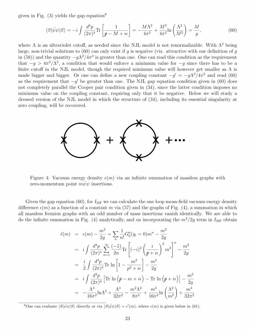
given in Fig. (3) yields the gap equation9
〈S|ψψ|S〉 = −i∫ d4p
(2π)4Tr
[1
/p−M + iε
]= −MΛ2
4π2+M3
4π2ln
(Λ2
M2
)=M
g, (60)
where Λ is an ultraviolet cutoff, as needed since the NJL model is not renormalizable. With Λ2 beinglarge, non-trivial solutions to (60) can only exist if g is negative (viz. attractive with our definition of gin (58)) and the quantity −gΛ2/4π2 is greater than one. One can read this condition as the requirementthat −g > 4π2/Λ2, a condition that would enforce a minimum value for −g since there has to be afinite cutoff in the NJL model, though the required minimum value will however get smaller as Λ ismade bigger and bigger. Or one can define a new coupling constant −g′ = −gΛ2/4π2 and read (60)as the requirement that −g′ be greater than one. The NJL gap equation condition given in (60) doesnot completely parallel the Cooper pair condition given in (34), since the latter condition imposes nominimum value on the coupling constant, requiring only that it be negative. Below we will study adressed version of the NJL model in which the structure of (34), including its essential singularity atzero coupling, will be recovered.
Figure 4: Vacuum energy density ε(m) via an infinite summation of massless graphs withzero-momentum point mψψ insertions.
Given the gap equation (60), for IMF we can calculate the one loop mean-field vacuum energy densitydifference ε(m) as a function of a constant m via (57) and the graphs of Fig. (4), a summation in whichall massless fermion graphs with an odd number of mass insertions vanish identically. We are able todo the infinite summation in Fig. (4) analytically, and on incorporating the m2/2g term in IMF obtain
ε(m) = ε(m)− m2
2g=∑n
1
n!Gn
0 (qi = 0)mn − m2
2g
= i∫ d4p
(2π)4
∞∑n=1
(−1)
2nTr
(−i)2
(i
/p+ iε
)2
m2
n − m2
2g
=i
2
∫ d4p
(2π)4Tr ln
[1− m2
p2 + iε
]− m2
2g
= i∫ d4p
(2π)4
[Tr ln
(/p−m+ iε
)− Tr ln
(/p+ iε
)]− m2
2g
= − Λ4
16π2lnΛ2 +
Λ4
32π2− m2Λ2
8π2+
m4
16π2ln
(Λ2
m2
)+
m4
32π2
9One can evaluate 〈S|ψψ|S〉 directly or via 〈S|ψψ|S〉 = ε′(m), where ε(m) is given below in (61).
23
−[− Λ4
16π2lnΛ2 +
Λ4
32π2
]+m2Λ2
8π2− m2M2
8π2ln
(Λ2
M2
)
=m4
16π2ln
(Λ2
m2
)− m2M2
8π2ln
(Λ2
M2
)+
m4
32π2. (61)
While the energy density 〈Ωm|Hm|Ωm〉/V = i∫d4p/(2π)4Tr ln[γµpµ −m] of Hm has quartic, quadratic
and logarithmically divergent pieces, the subtraction of the massless vacuum energy density given as〈Ω0|H0|Ω0〉/V = 〈Ω0|Hm|Ω0〉/V = i
∫d4p/(2π)4Tr ln[γµpµ] removes the quartic divergence, with the
subtraction of the self-consistent induced mean-field term m2/2g then leaving ε(m) only logarithmicallydivergent. We recognize the resulting logarithmically divergent ε(m) as having a local maximum atm = 0, and a global minimum at m = M where M itself is finite. We thus induce none other thana dynamical double-well Mexican Hat potential, and identify M as the matrix element of a fermionbilinear according to M/g = 〈S|ψψ|S〉. In arriving at this result we note the power of dynamicalsymmetry breaking: it generates a −m2/2g counterterm automatically, with the quadratic divergencein 〈Ωm|Hm|Ωm〉/V being canceled without our needing to introduce a counterterm by hand. This pointis particularly significant since for an elementary Higgs field the one loop self-energy contribution isquadratically divergent, to thus naturally be of order some high cutoff scale (the so-called hierarchyproblem) rather than the typical weak interaction breaking scale that it is now known to have.
If instead of looking at matrix elements in the translationally-invariant vacuum |S〉 we instead lookat matrix elements in coherent states |C〉 where m(x) = 〈C|ψ(x)ψ(x)|C〉 is now spacetime dependent,10
we then obtain [34, 35] a mean-field effective action IEFF = W (m(x)) of the form
IEFF = iTrln
[i/∂x −m(x)
i/∂x
]
=∫d4x
[1
8π2ln
(Λ2
M2
)(1
2∂µm(x)∂µm(x) +m2(x)M2 − 1
2m4(x)
)+ ....
], (62)
where we have explicitly displayed the leading logarithmically divergent part. Here the kinetic energyterm is the analog of the Z(J) term given earlier in the expansion of W (J) around the point whereall momenta vanish. In terms of the quantity ΠS(q2,M) to be given below in (67), Z(M) is given by∂ΠS(q2,M)/∂q2|q2=0 = (1/8π2)ln(Λ2/M2).11 If we introduce a coupling gAψγµγ
5Aµ5ψ to an axial gaugefield Aµ5(x), on setting φ(x) = 〈C|ψ(1 + γ5)ψ|C〉 the effective action becomes
IEFF =∫ d4x
8π2ln
(Λ2
M2
) [1
2|(∂µ − 2igAAµ5)φ(x)|2 + |φ(x)|2M2 − 1
2|φ(x)|4 − g2
A
6Fµν5F
µν5]. (63)
10Such coherent states can be generated from the self-consistent vacuum |Ωm〉 by a spacetime-dependent Bogoliubovtransform [33], and lead with elementary scalar field vacuum breaking [33] or bilinear fermion vacuum breaking [29] toextended, bag-like, states where a positive energy fermion is localized by its own negative energy sea. (In [29] it wassuggested that the bag pressure of such bag-like states could serve as the electrodynamical Poincare stresses mentionedin Sec. (1.2) as now generated dynamically in the vacuum.) For static, spherically symmetric extended structures m(x)would only depend on the radius and thus be an even function of x. With its spatial trace in (62), IEFF can be writtenas IEFF = iTrln[i/∂x −m(x)] − iTrln[i/∂x] = iTrln[i/∂x −m(x)]/2 − iTrln[i/∂x]/2 +iTrln[−i/∂x −m(x)]/2 − iTrln[−i/∂x]/2= iTrln[∂2
x + m2(x)]/2 − iTrln[∂2x]/2. Thus, in analog with (12), in the presence of such extended structures and with
m(x) being real, IEFF would be real to all orders in derivatives of m(x). With a constant m(x) also being symmetric, werecover our previous observation that IEFF, and thus ε(m), would be real if m(x) is constant.
11As noted in [35], the full expansion for IEFF involves all higher-order derivatives of m(x), with each coefficientin the expansion being given by an appropriate derivative of a momentum-space Feynman diagram as calculated with aconstant m that is then replaced by m(x) after the integration. (Π′′S(q2 = 0,m))|m=m(x) for instance gives the coefficient of[2m(x)]2. While such an all-derivative expansion does not violate locality if m(x) is a c-number field since the underlyingfour-fermion theory that produced it is local, an all-derivative expansion would violate locality for a q-number scalar field,to thus underscore the distinction between dynamical and elementary Higgs fields.
24

We recognize this action as being a double-well Ginzburg-Landau type Higgs Lagrangian, only nowgenerated dynamically. We thus generalize to the relativistic chiral case Gorkov’s derivation of theGinzburg-Landau order parameter action starting from the BCS four-fermion theory. In the IEFF
effective action associated with the NJL model there is a double-well Higgs potential, but since theorder parameter m(x) = 〈C|ψ(x)ψ(x)|C〉 is a c-number, m(x) does not itself represent a q-numberscalar field. And not only that, unlike in the elementary Higgs case, the second derivative of V (m(x))at the minimum where m = M is not the mass of a q-number Higgs boson. Rather, as we now show,the q-number fields are to be found as collective modes generated by the residual interaction, and itis the residual interaction that will fix their masses. Moreover, as we will see in Sec. (8), when wedress the point NJL vertices that are exhibited in Figs. (3), (4), and (5), the dynamical Higgs bosonwill move above the threshold in the fermion-antifermion scattering amplitude, become unstable, andacquire a width. Since this same dressing of the point NJL vertices will lead to a modified effectiveGinzburg-Landau V (m(x)), and since this V (m(x)), and thus its second derivative at its minimum willbe real, we see that because of the collective mode Higgs boson width we could not even in principlerelate the value of the second derivative of V (m(x)) to the collective mode Higgs mass produced by theresidual interaction. Since, the (radiatively dressed) Hermitian Higgs potential for an elementary Higgsboson is real, the width of the Higgs boson has the potential to discriminate between an elementaryHiggs boson and a dynamical one.
6.3 The Collective Scalar and Pseudoscalar Tachyon Modes
To find the collective modes we calculate the scalar and pseudoscalar sector Green’s functions ΠS(x) =〈Ω|T [ψ(x)ψ(x)ψ(0)ψ(0)]|Ω〉, ΠP(x) = 〈Ω|T [ψ(x)iγ5ψ(x)ψ(0)iγ5ψ(0)]|Ω〉, as is appropriate to a chiral-invariant theory. If first we take the fermion to be massless (i.e. setting |Ω〉 = |Ω0〉 = |N〉 where〈N |ψψ|N〉 = 0), to one loop order in the four-fermion residual interaction we obtain
ΠS(q2,m = 0) = i∫ d4p
(2π)4Tr[
1
/p+ iε
1
/p+ /q + iε
]= − 1
8π2
(2Λ2 + q2ln
(Λ2
−q2
)+ q2
),
ΠP(q2,m = 0) = i∫ d4p
(2π)4Tr[iγ5 1
/p+ iεiγ5 1
/p+ /q + iε
]= − 1
8π2
(2Λ2 + q2ln
(Λ2
−q2
)+ q2
). (64)
On iterating the residual interaction, the scattering matrices in the scalar and pseudoscalar channelsare given by
TS(q2,m = 0) =g
1− gΠS(q2,m = 0)=
1
g−1 − ΠS(q2,m = 0),
TP(q2,m = 0) =g
1− gΠP(q2,m = 0)=
1
g−1 − ΠP(q2,m = 0). (65)
and with g−1 being given by the gap equation (60), near q2 = −2M2 both scattering matrices behaveas
TS(q2,M = 0) = TP(q2,M = 0) =Z−1
(q2 + 2M2), Z =
1
8π2ln
(Λ2
M2
). (66)
We thus obtain degenerate (i.e. chirally-symmetric) scalar and pseudoscalar tachyons at q2 = −2M2
(just like fluctuating around the local maximum in a double-well potential), with |N〉 thus being un-stable.
25

Figure 5: ΠS(q2,m) developed as an infinite summation of massless graphs, each with twopoint mψψ insertions carrying momentum qµ (shown as external lines), with all other pointmψψ insertions carrying zero momentum.
6.4 The Collective Goldstone and Higgs Modes
However, suppose we now take the fermion to have nonzero mass M (i.e. we set |Ω〉 = |Ωm〉 = |S〉where 〈S|ψψ|S〉 6= 0). As per the summation for ΠS(q2,m) given in Fig. (5) and its ΠP(q2,m) analog,we obtain
ΠP(q2,M) = −i∫ d4p
(2π)4Tr[iγ5 1
/p−m+ iεiγ5 1
/p+ /q −m+ iε
]
= − Λ2
4π2+M2
4π2ln
(Λ2
M2
)− q2
8π2ln
(Λ2
M2
)− (q2 − 4M2)
8π2
− (8M4 − 8M2q2 + q4)
8π2q2
(−q2
4M2 − q2
)1/2
ln
((4M2 − q2)1/2 + (−q2)1/2
(4M2 − q2)1/2 − (−q2)1/2
),
ΠS(q2,M) = −i∫ d4p
(2π)4Tr[
1
/p−m+ iε
1
/p+ /q −m+ iε
]
= − Λ2
4π2+M2
4π2ln
(Λ2
M2
)+
(4M2 − q2)
8π2ln
(Λ2
M2
)+
(4M2 − q2)
8π2
− (4M2 − q2)
8π2
(4M2 − q2
−q2
)1/2
ln
((4M2 − q2)1/2 + (−q2)1/2
(4M2 − q2)1/2 − (−q2)1/2
), (67)
with both of these Green’s functions having a branch point at q2 = 4M2, which for a fermion of massM , is right at the threshold in the fermion-antifermion scattering amplitude. Given the form for g−1,we find a dynamical pseudoscalar Goldstone boson bound state in TP(q2,M) at q2 = 0 and a dynamicalscalar Higgs boson bound state in TS(q2,M) at q2 = 4M2 (= −2×M2(tachyon)).12 Near the respectivepoles the scattering amplitudes behave as:
TS(q2,M) =Z−1
S
(q2 − 4M2), TP(q2,M) =
Z−1P
q2, ZS = ZP =
1
8π2ln
(Λ2
M2
). (68)
The two dynamical bound states are not degenerate in mass (spontaneously broken chiral symmetry),and the dynamical Higgs scalar mass 2M is twice the induced mass of the fermion, to thus lie right atthe scattering amplitude threshold.
12As noted in [36, 37], the Higgs mechanism that holds for an elementary Higgs field generalizes to the dynamical case,with a dynamical Goldstone boson automatically giving a mass to the gauge boson associated with any local currentto which the Goldstone boson may couple. It will thus suffice for our purposes here to show that there is a dynamicalGoldstone boson to begin with.
26
Now stationary solutions to IEFF given in (62) obey
2m(x)− 2m(x)M2 + 2m3(x) = 0. (69)
We can associate this wave equation with a potential
V (m) =1
2m4(x)−m2(x)M2, (70)
with its first derivative vanishing at m = M , and its second derivative being the positive V ′′(M) = 4M2
at m = M . With fluctuations around m = M taking the form m = M + χ, for such fluctuations thepotential takes the form:
V (M + χ) = −1
2M4 +
1
2(4M2)χ2 + 2Mχ3 +
1
2χ4. (71)
to thus describe a scalar fluctuation with positive mass squared equal to 4M2. Now while this 4M2
mass squared happens to be equal to the dynamical Higgs boson mass squared as given in (68), suchan equality is not generic, since, as we see below, once one dresses the vertices these squared massesdo not remain equal. Thus one cannot use a dressed Ginzburg-Landau action to determine the Higgsmass, one must use the dressed scattering amplitude.
A very significant aspect of (68) is that the pole in TS(q2,M) is at q2 = 4M2, i.e. at a location thatdoes not depend on the cutoff Λ that the NJL model needs. Thus when the Higgs boson is dynamicalits mass can naturally be of order the dynamical fermion mass M and not be of order the cutoff scale, asboth the fermion and Higgs boson masses are generated by one and the same chiral symmetry breakingmechanism. This is very different from the elementary Higgs case where the Higgs boson self-energy isof order the cutoff scale, and there is no relation between the Higgs boson mass scale and the massesof fermions that arise through their Yukawa couplings to the self-same Higgs boson.
A second significant feature of (68) is that the residue at the pole in TS(q2,M), and thus the couplingof a dynamical Higgs boson to a fermion-antifermion pair, is completely determined by the dynamics.This is in sharp contrast to the elementary Higgs boson situation where fundamental Yukawa couplingsare totally unconstrained. One of the central shortcomings of the standard elementary Higgs field theoryis that the tree approximation minimum to the Higgs potential is determined by the Higgs sector alone,with the Yukawa-coupled fermions playing no role at the tree level. And since the fermions do play norole, the strengths of the Yukawa coupling terms are totally unconstrained. However, in the dynamicalHiggs case it is the interaction of the fermions that determines where the Higgs bound state pole is tolie, while at the same time determining its residue, i.e. its coupling to a fermion-antifermion pair. Thusif one wants to be able to determine the strengths of the Yukawa coupling terms, the fermions wouldhave to play an explicit role in generating the Higgs boson in the first place.
As a model the NJL model is very instructive since it captures the key features of dynamicalsymmetry breaking. However its drawback is that the NJL model is not renormalizable. We thus nowturn to a discussion of dynamical symmetry breaking in some specific theories that are renormalizable.
7 The Abelian Gluon Model
7.1 The Schwinger-Dyson Equation
The Abelian gluon model is based on the same action as QED, viz.
IQED =∫d4x
[−1
4FµνF
µν + ψγµ(i∂µ − e0Aµ)ψ −m0ψψ], (72)
27

but without the requirement that e0 necessarily be the bare electric charge. This permits considerationof both strong and weak coupling. Though we are interested in dynamical mass generation we haveincluded a bare mass term in (72) as this will enable us to monitor the nature of the mass generation.In the theory the exact inverse fermion propagator S−1(p) = /p − m0 − Σ(p) obeys the exact, as yetunrenormalized, all-order, Schwinger-Dyson equation
Σ(p) = ie20
∫ d4q
(2π)4Dµν(p− q)Γµ(p, q)S(q)γν , (73)
where Dµν(p−q) and Γµ(p, q) are the exact gluon propagator and exact fermion-antifermion-gluon vertexfunction. Starting with the work of Johnson, Baker, and Willey [38, 39, 40, 41, 42, 43] there has beenmuch interest in finding self-consistent solutions to this Schwinger-Dyson equation. We shall discuss thework of Johnson, Baker, and Willey below but shall first discuss the quenched, planar approximationtreatment since it is very instructive. This approximation is referred to as being quenched because thegluon propagator is taken to be the bare propagator (i.e. no charge renormalization), and is planar sincethe only gluon exchange diagrams that are taken to contribute to the fermion propagator are those inwhich no two gluon lines cross each other. (Thus one keeps graphs such as the first two graphs in Fig.(6) and their higher order analogs but not those such as the third graph or its higher order analogs.)The approximation is also called the ladder approximation or the rainbow graph approximation becauseof the pictorial form of the graphs. Some early studies of the quenched planar approximation may befound in [44, 45, 46, 47], with detailed reviews and full references being provided in [32] and [48].
Figure 6: The first few graphs in the fermion self-energy Schwinger-Dyson equation
In general because of its Lorentz structure one can set S−1(p) = A(p2)/p − B(p2) where A(p2) andB(p2) are Lorentz scalars. In the quenched planar approximation it is convenient to initially work ina general covariant gauge in which Dµν(k) = (ξkµkν/k
2 − ηµν)/k2 where ξ is a constant. Then, sinceΓµ(p, q) is equal to γµ in this approximation, the Schwinger-Dyson equation takes the form
/p[1− A(p2)] +B(p2) = m0 + ie2∫ d4q
(2π)4
(ξ − 4)B(q2)
(p− q)2[A2(q2)q2 −B(q2)]
+ ie2∫ d4q
(2π)4
A(q2)[2ξ(/p− /q)(p · q − q2) + (2− ξ)/q(p− q)2]
(p− q)4[A2(q2)q2 −B(q2)]. (74)
In (74) we have replaced the bare charge e0 by the physical charge e since there is no charge renormal-ization.
On transforming to Euclidean space, we introduce angular coordinates q1 = q sinψ sin θ cosφ, q2 =q sinψ sin θ sinφ, q3 = q sinψ cos θ, q4 = q cosψ, where 0 ≤ ψ ≤ π, 0 ≤ θ ≤ π, 0 ≤ φ ≤ 2π, andwhere the volume element is dqdψdθdφq3 sin2 ψ sin θ. For the dependence on pµ we conveniently setpµ = (0, 0, 0, p). Then, with p ·q = pq cosψ, (p−q)2 = p2−2pq cosψ+q2, we find that on the right-handside of (74) the only dependence on θ and φ is in the γ1q1, γ2q2, and γ3q3 terms. On doing the dθdφintegration all of the integrals that contain these terms are found to vanish identically, doing so in factfor arbitrary ξ. For arbitrary ξ the term proportional to γ4 does not vanish on doing the remaining
28
angular integration viz. that on ψ, but does conveniently vanish in the Landau gauge where ξ = 1.13
With there then being no dependence on A(p2) in the numerator of the second integral on the right-handside of (74), from the structure of the left-hand side we conclude that in the Landau gauge A(p2) = 1[38]. In the Landau gauge (74) thus takes the form
B(p2) = m0 +3e2
8π3
∫ ∞0
q2dq2∫ π
0dψ sin2 ψ
B(q2)
(p2 + q2 − 2pq cosψ)[q2 +B2(q2)]
= m0 +3e2
8π3
∫ ∞0
q2dq2 B(q2)
[q2 +B2(q2)]
π
4p2q2
(p2 + q2 − (p2 − q2)2
|p2 − q2|
), (75)
to thus take the form in which it commonly appears in the quenched ladder approximation literature,viz.
B(p2) = m0 +3α
4π
[ ∫ p2
0dq2 q2B(q2)
p2[q2 +B2(q2)]+∫ ∞p2
dq2 B(q2)
[q2 +B2(q2)]
], (76)
where α = e2/4π.On cutting off the q2 integration at Λ2, a convergent asymptotic solution of the form B(p2) =
m(p2/m2)(ν−1)/2 is found for (76) with
ν = ±(
1− 3α
π
)1/2
, m0 =3αm
2π(1− ν)
Λν−1
mν−1, (77)
with ν being real provided α ≤ π/3.14 With ν having a branch point at α = π/3, we can thus anticipatethat a phase transition might occur at that value of the coupling constant. While the above solutiongives a real ν if α ≤ π/3, if α > π/3 we would instead obtain B(p2) ∼ (p2)−1/2 exp(±i(µ/2)ln(p2/m2))where µ = (3α/π− 1)1/2. This then gives two classes of real solutions, viz. (p2)−1/2 cos[(µ/2)ln(p2/m2)]and (p2)−1/2 sin[(µ/2)ln(p2/m2)]. Combining them gives the α > π/3 asymptotic solution
B(p2) =m cos[((3α/π − 1)1/2/2)ln(p2/m2) + σ]
(p2/m2)1/2, m0 = −3mα cos[(3α/π − 1)1/2ln(Λ/m) + τ ]
2π(µ2 + 1)1/2(Λ/m), (78)
where σ is a (possibly Λ2/m2 but not p2/m2 dependent) phase and τ = σ + arctanµ. As required, wesee that for both α ≤ π/3 and α > π/3 the bare mass vanishes in the limit in which the cutoff goes toinfinity. However, as we elaborate on below, that does not mean that the bare mass is identically zero,only that it vanishes in the limit of infinite cutoff. For α ≤ π/3 this is the only option for the baremass. However for α > π/3 there is a second option for the bare mass, since it will vanish identically ifwe set (
3α
π− 1
)1/2
ln(Λ/m) + τ =π
2. (79)
Now initially this would suggest that as we let Λ go to infinity, the only allowed value for α would beα = π/3. In order to be able to obtain a solution that is to hold for all α > π/3, we take τ to be of theform τ = δln(Λ/m) where δ is finite, so that we obtain(
3α
π− 1
)1/2
+ δ =π
2ln(Λ/m), (80)
13To show this when ξ = 1, we note that 2(p4− q4)(p · q− q2) + q4(p− q)2 = −2pq2 + 3q(p2 + q2) cosψ−4pq2 cos2 ψ. Onintroducing I0 = (1/π)
∫ π0dψ/(p2 + q2 − 2pq cosψ) = 1/|p2 − q2|, In = (1/π)
∫ π0dψ sin2 ψ cosn−1 ψ/(p2 + q2 − 2pq cosψ)2
with I1 = [(p2 + q2)I0 − 1]/4p2q2, I2 = [2(p2 + q2)2I0 − 4p2q2I0 − 2p2 − 2q2]/8p3q3, I3 = [3(p2 + q2)3I0 − 8p2q2(p2 +q2)I0 + 2p2q2 − 3(p2 + q2)2]/16p4q4, we find that −2pq2I1 + 3q(p2 + q2)I2 − 4pq2I3 = 0. With this cancellation occurringidentically without needing to specify any actual form for I0, and with I0 actually behaving as 1/|p2−q2|, the cancellationoccurs in (74) for all values of the integration variable q, i.e. for q greater than, equal to, or lesser than p.
14The power solution to (75) of the form B(p2) = (p2)(ν−1)/2 with ν as given in (77) was first presented in [38].
29
and thus
B(p2) =m cos[((3α/π − 1)1/2/2)ln(p2/Λ2)− arctanµ+ π/2]
(p2/m2)1/2, m0 = 0. (81)
Then, with δ being an appropriately chosen function of α, all values of α greater than π/3 are allowed inthe limit of infinite cutoff.15 Since for all such values of α the bare mass is identically zero, for α > π/3dynamical symmetry breaking will take place for any non-trivial solution to
B(p2) = 3e2∫ d4q
(2π)4
B(q2)
(p− q)2(q2 +B2(q2))(82)
that behaves asymptotically as in (81).16 Thus for all values of α greater than π/3 (i.e. strong coupling),the quenched ladder approximation has a chiral symmetry that is broken dynamically, with dynamicalGoldstone boson generation taking place [44, 45, 46, 47]. With the asymptotic solution possessing abranch point at α = π/3, we can anticipate that the behavior of the theory below α = π/3 will bequalitatively different from its behavior above α = π/3. Thus to discuss what happens when α is belowπ/3 we turn to a renormalization group analysis.
7.2 Renormalization Group Analysis
In the Abelian gluon model it was shown [50, 51] that the renormalized inverse fermion propagatorS−1(p,m) and the renormalized vertex function ΓS(p, p, 0,m) associated with the insertion of the com-posite operator θ = ψψ with zero momentum into the inverse fermion propagator are related by therenormalization group equation[
m∂
m+ β(α)
∂
∂α
]S−1(p,m) = −m[1− γθ(α)]ΓS(p, p, 0,m) (83)
in the limit in which the fermion momentum pµ is deep Euclidean. In (83) β(α) is associated withcoupling constant renormalization, and γθ(α) is the anomalous dimension associated with the operatorψψ, defined here so that the total dimension of ψψ is given by dθ(α) = 3+γθ(α) where 3 is the canonicalvalue.17 In any situation in which β(α) = 0, this equation admits of an exact asymptotic solution
S−1(p,m) = /p−m(−p2 − iεm2
)γθ(α)/2
+ iε, ΓS(p, p, 0,m) =
(−p2 − iεm2
)γθ(α)/2
, (84)
one that converges asymptotically if γθ(α) is negative. Asymptotic convergence is thus achieved ifdynamically dθ(α) is less than canonical.
There are two standard ways to achieve β(α) = 0. The first is to only have β(α) vanish for somespecific value of α, the Gell-Mann-Low eigenvalue condition. It is this particular possibility that wasexplored by Johnson, Baker, and Willey, and will be discussed below. The second is to use the quenched
15A ln(Λ/m) dependence to the phase τ seems not to have been considered in the quenched ladder approximationliterature, where instead one restricts [49] to (3α/π−1)1/2 = π/2ln(Λ/m), a quantity that vanishes in the limit of infinitecutoff, to then not permit α to take any value other than π/3.
16We note that while the asymptotic solution given for B(p2) in (77) is cutoff independent, the solution given in (81)does depend on the cutoff (as would the solution for B(p2) given in (78) if we were to set (3α/π − 1)1/2 = π/2ln(Λ/m)).Consequently, solutions to the quenched ladder approximation Schwinger-Dyson equation can only be cutoff independentif α ≤ π/3.
17A possible anomalous dimension γF term for the fermion has been removed from (83) via a judicious choice of gauge.Also we note that in the critical scaling literature the dimension and anomalous dimension of dθ(α) are sometimes denotedby dm and γm, and defined via dm = 3− γm.
30
approximation described above since then the coupling constant is not renormalized for any value of α,with β(α) vanishing for every value of α. Comparing (83) with (77), we see that the asymptotic solutionfound in the quenched ladder approximation exactly scales as a power in the α ≤ π/3 region just asthe renormalization group requires, to thus yield the identification ν − 1 = γθ(α). At the critical valueα = π/3 we note that γθ(α) = −1, so that dθ(α) = 2. We shall have occasion to return to this valuefor dθ(α) below while noting now that with it (ψψ)2 acts as an operator whose dimension is reducedfrom six to four, i.e. to the value that would make the four-fermion interaction be power-countingrenormalizable.
We can also use the renormalization group equation in the α > π/3 region, and inserting eitherB(p2) ∼ (p2)−1/2 exp(+i(µ/2)ln(p2/m2)) or B(p2) ∼ (p2)−1/2 exp(−i(µ/2)ln(p2/m2)) into (83) yields
Re[γθ(α > π/3)] = −1, (85)
with the real part of γθ(α), viz. the part that controls the asymptotic behavior of the propagator, thusbeing equal to −1 for all α > π/3.18 In this respect the phase transition at α = π/3 is one in whichRe[γθ(α)] varies continuously from zero to one as α varies continuously from zero to π/3, but then staysat one when α is greater than π/3, with there thus being a discontinuity in γθ(α) at α = π/3, even asthere is none in β(α). One should expect a discontinuity in γθ(α) rather in β(α), since it is θ = ψψthat is the mass operator. Thus if any discontinuity is to herald a dynamical mass generation phasetransition, it should be in the mass operator sector rather than in the charge operator sector.
7.3 Johnson-Baker-Willey Electrodynamics
The objective of the study of Johnson, Baker, and Willey [38, 39, 40, 41, 42, 43] was not to studydynamical symmetry breaking per se, but to determine whether it might be possible for all the renor-malization constants of a quantum field theory to be finite. Quantum electrodynamics was a particularlyconvenient theory to study since its gauge structure meant that two of its renormalization constants(the fermion wave function renormalization constant Z2 and the fermion-antifermion-gauge boson ver-tex renormalization constant Z1 to which Z2 is equal) were gauge dependent and could be made finiteby an appropriate choice of gauge, with the anomalous dimension of the fermion γF associated with Z2
consequently then being zero. Johnson, Baker, and Willey were thus left with the gauge boson wavefunction renormalization constant Z3 and the fermion bare mass m0 and its shift δm to address.
Now if one were also to consider the coupling of electrodynamics to gravity, one would then have toaddress another infinity that electrodynamics possesses, namely that of the zero-point vacuum energydensity, and we will return to this issue below. However, in the flat spacetime study that Johnson,Baker, and Willey engaged in, the need to address the vacuum energy density infinity did not arise,and it could be normal ordered away.
As regards Z3 and m0, Johnson, Baker and Willey showed that Z3 would be finite if the fermion-antifermion-gauge boson coupling constant α was at a solution to the Gell-Mann-Low eigenvalue con-dition. At this eigenvalue they showed that the fermion propagator would scale asymptotically as in
18As noted above, in [49] (79) was solved with finite τ , to thus lead to (3α/π−1)1/2 = π/2lnΛ. On defining an effectivebeta function according to β(α) = Λ∂Λα(Λ), this particular β(α) evaluates (see e.g. [52]) to β(α) = −(2/3)(3α/π−1)3/2,to thus permit use of the α > π/3 region renormalization group analysis given in studies such as that of [53]. However,as noted in [52], whatever this effective beta function is, it cannot be associated with charge renormalization, sincethere is no charge renormalization in the quenched ladder approximation even in the α > π/3 region. Rather, as weindicate here, one should stay with the vanishing of the standard charge renormalization beta function, and then use thestandard renormalization group equation given as (83) in the α > π/3 region. Curiously though, we note that standardrenormalization group procedure and that presented in [53] both lead to Re[γθ(α > π/3)] = −1 in the entire α > π/3region, though in the discussion presented in [53] one additionally has Im[γθ(α > π/3)] = 0.
31

(84), and that the bare mass would scale as
m0 = m
(Λ2
m2
)γθ(α)/2
, (86)
where Λ is an ultraviolet cutoff and m = m0 + δm is the renormalized fermion mass. Consequently ifthe power γθ(α) is negative (which it perturbatively is: γθ(α) = −3α/2π− 3α2/16π2 + O(α3)), the baremass would vanish in the limit of infinite cutoff and δm would be finite. Thus the mechanism for boththe finiteness and vanishing of m0 is to have the dimension of ψψ be less than canonical.19 As such,the work of Johnson, Baker, and Willey was quite remarkable since it predated the work of Wilson andof Callan and Symanzik on critical scaling, anomalous dimensions, and the renormalization group.
7.4 The Baker-Johnson Evasion of the Goldstone Theorem
With the vanishing of the bare mass and the non-vanishing of the physical mass, it looks as though thereshould be dynamical mass generation and an associated Goldstone boson, with JBW electrodynamicsthen becoming a possible laboratory in which to explore dynamical symmetry breaking. However,this turned out not to be the case due to a hidden renormalization effect in the theory [41], one
associated with the renormalization constant Z−1/2θ = (Λ2/m2)γθ(α)/2 that renormalizes ψψ according
to Z−1/2θ (ψψ)0 = ψψ [50]. Specifically, given (86), it follows that as m0 vanishes the quantity (ψψ)0
diverges at the same rate so that m0(ψψ)0 = mZ−1/2θ Z
1/2θ ψψ = mψψ is finite. Then if m is non-zero, the
bare m0(ψψ)0 is non-zero too. The solution associated with (86) thus corresponds to a theory in whicha term m0(ψψ)0 is present in the Lagrangian from the outset. The chiral symmetry is thus broken inthe Lagrangian and there is no associated Goldstone boson. This then is the evasion of the Goldstonetheorem as found by Baker and Johnson [41].
Since the Baker-Johnson evasion of the Goldstone theorem would hold in any theory in which thebare mass has a negative power dependence on the cutoff, it follows that this must also be the casein the quenched ladder approximation to the Abelian gluon model in the α ≤ π/3 region. Hence thebranch point in ν at α = π/3 separates two distinct phases. At or below α = π/3 there is no Goldstoneboson, while above α = π/3 there is. Now suppose that a priori one did not know whether or not theBaker-Johnson evasion of the Goldstone theorem applied below α = π/3. If one had set the bare massequal to zero in an equation such as (74) right at the beginning of the calculation, one would havecome to the conclusion that with an identically zero m0 and the power-behaved solution given in (77),equation (74) would exist without renormalization and lead to self-consistent mass generation. Onewould thus have concluded that even in the α ≤ π/3 region there should be a Goldstone boson, with aself-consistently non-zero B(p2), and a self-consistently non-zero fermion mass, generating themselvesin the Schwinger-Dyson equation. However, if we first introduce both a bare mass and a cutoff andthen solve (74) asymptotically, we would find that for α ≤ π/3 the bare mass as given in (77) wouldactually be non-zero. Then with m0 as given in (77) vanishing in the limit of infinite cutoff we wouldknow that we are in fact in the Baker-Johnson situation. Thus to check whether or not we might be inthe Baker-Johnson situation, even if we are in a renormalizable and seemingly chiral-symmetric theory,we should nonetheless study the Schwinger-Dyson equation with a cutoff.20
19If we expand m0 in (86) we obtain m0/m = 1 + γθ(α)ln(Λ/m) + (γ2θ (α)/2)ln2(Λ/m) + .... Even though each term in
the series diverges, their coefficients are fixed by the vanishing of β(α) so that the series exponentiates.20We had noted above that one can obtain the Schwinger-Dyson equation via the stationarity condition δΓ(G)δG(x, y) =
0 associated with the bilinear source K(x, y) approach presented in [27]. While this would then permit self-consistent non-trivial solutions to the Schwinger-Dyson equation, this would not necessarily mean that in them the bare mass would beidentically zero and that one would have dynamical symmetry breaking, since if one has an asymptotically power-behavedsolution to the Schwinger-Dyson equation, one would be in the Baker-Johnson situation where despite appearances the
32
With the realization that there is no Goldstone boson when α ≤ π/3, the prevailing wisdom thatthen ensued from the quenched ladder approximation study is that Goldstone boson generation isstrictly a strong coupling effect, with the α ≤ π/3 region not being of relevance to dynamical symmetrybreaking. Below we shall revisit this issue and show that it is possible to generate Goldstone and Higgsbosons dynamically even if the coupling is weak. To do this we will need to couple a weakly coupledQED to an equally weakly coupled four-fermion interaction. However, before doing this we need to askhow reliable a guide to dynamical symmetry breaking the quenched ladder approximation actually is.
7.5 The Shortcomings of the Quenched Ladder Approximation
To determine how relevant the wisdom obtained from the quenched planar approximation to the Abeliangluon model might be for the full theory, we need to include the non-planar graphs and need to dressthe gluon propagator. Inclusion of all the Feynman graphs was the objective of Johnson, Baker, andWilley in their study of quantum electrodynamics. In their study of quantum electrodynamics Johnson,Baker, and Willey initially kept the photon propagator canonical [38] (i.e. no internal fermion loops inthe photon propagator) with the photon propagator thus being quenched, but they otherwise includedboth planar and non-planar graphs to all orders, to thus include the full Γµ(p, p − k) vertex in theSchwinger-Dyson equation rather than just its undressed γµ approximation. In [38] they then found thatthe fermion self-energy then scaled asymptotically just as in (84), i.e. as (−p2/m2)γθ(α)/2. Moreover,Johnson, Baker and Willey noted that their analysis only depended on the asymptotic momentumbehavior of Feynman diagrams and not on the strength of the coupling. Their analysis thus holdsfor both weak and strong coupling, and as such shows no region in which a power-behaved solutionchanges into an oscillating one such as the one exhibited in (78), with the power-behaved, and thusnon-Goldstone mode, solution holding for all values of the coupling constant. Thus in the quenchedbut otherwise all-order approximation to the Abelian gluon model, the phase transition at α = π/3 inthe planar approximation is nullified by the non-planar graphs, and one has to conclude that in the fullplanar plus non-planar quenched gluon approximation there is no Goldstone boson.
As had been noted above, in the quenched ladder approximation we keep graphs such as the first twographs in Fig. (6) and their higher-order planar analogs but do not include the non-planar third graphor its higher-order non-planar analogs. However, the second and the third graphs in Fig. (6) are of thesame order in α. With the third graph being a factor of α weaker than the first graph in the figure, andwith the three-gluon non-planar graph (not shown) being a factor of α weaker than the second graph inthe figure, we see that compared to the planar graphs the non-planar graphs are suppressed by a factorof α. Their neglect is thus only valid if the coupling is weak. The quenched planar approximation isthus strictly a weak coupling approximation, with its application in the strong coupling regime whereα is of order π/3 potentially not being valid, and with the strong coupling wisdom that is gleaned fromthe quenched ladder approximation not being reliable.
To see exactly at what point the quenched ladder approximation begins to depart from the quenched,all-order Johnson-Baker-Willey (JBW) study reported in [38], we note that through second order in αthe contribution of all graphs gives [38] γθ(α) = −3α/2π−3α2/16π2, whereas, as per (77), the expansionof ν−1 = (1−3α/π)1/2−1 to second order is given by −3α/2π−9α2/8π2. Thus, as can be anticipatedfrom the graphs in Fig. (6), already at the level of the two-photon graphs γθ(α) and ν − 1 begin todepart from each other, and yet the compatibility of (77) and (84) would require that γθ(α) and ν − 1be equal. The extrapolation of the ν − 1 = (1 − 3α/π)1/2 − 1 expression beyond lowest order is thusnot justifiable, with the branch point obtained in ν at α = π/3 in the quenched planar approximation
chiral symmetry would actually be broken in the Lagrangian. In and of itself the effective action approach of [27] doesnot distinguish between a bare mass that is zero and one that only vanishes in the limit of infinite cutoff, as this isdeterminable not from the form of the unconstrained action itself but from the structure of its stationary solution.
33
being an indicator not that there is a phase transition, but that the extrapolation is problematic.21
In [39] Johnson, Baker, and Willey went further and actually justified the restriction to a canonicalphoton by noting that the photon would indeed be canonical if the coupling constant satisfied the Gell-Mann-Low eigenvalue condition, and thus satisfied β(α) = 0.22 Thus whether one takes the photon tobe quenched or takes it to couple with a charge that obeys β(α) = 0, in either case the power-behaved(−p2/m2)γθ(α)/2 asymptotic behavior is the only allowed solution, with there being no sign of any phasetransition. Moreover, if one is at the Gell-Mann-Low eigenvalue, the coupling constant would only haveone (or possibly a few) discrete values, with there then being no possibility of being able to vary α overthe entire coupling constant range and look for any discontinuity in the first place. Other than thefact that a zero of β(α) (should it have one) might be at a location other than α = π/3, the wisdomobtained in the quenched ladder approximation at α = π/3 does dovetail with that found by Johnson,Baker, and Willey at a Gell-Mann-Low eigenvalue, i.e. there is asymptotic scaling but no Goldstoneboson.23 As we will see, the correspondence is even stronger since in both the cases the dimension ofdθ(α) is reduced from three to two. In the quenched ladder approximation this follows directly from(77) at α = π/3, while in the Johnson, Baker, and Willey case it is, as we show below, the condition[28, 26] that the vacuum spontaneously break.
Figure 7: 〈Ωm|ψψ|Ωm〉 as constructed from the quenched ladder approximation fermionpropagator, which is represented as a blob.
Beyond the issue of the validity of the quenched ladder approximation, there may also be a possiblecounting issue. Specifically, if we want to calculate the one-point function expectation value 〈Ωm|ψψ|Ωm〉in the quenched ladder approximation, we would just sew together the two ends of the fermion prop-agator (cf. the planar part of Fig. (6)) to produce Fig. (7), this being the tadpole used in [52] forinstance. However, suppose we want to evaluate the three-point function 〈Ωm|T [ψ(x)ψ(z)ψ(z)ψ(y)]|Ωm〉in this same approximation. This would involve the planar graphs in Fig. (8) and their higher-order analogs but not the non-planar ones. Suppose we now want to evaluate the two-point function
21That a lowest order type calculation could lead to a phase transition that is only apparent is familiar from a study ofthe four-fermion theory in two dimensions with interaction −(g/2)(ψψ)2− (g/2)(ψiγ5ψ)2. With point ψψ couplings, onecould repeat the four-dimensional NJL calculation and conclude that there is dynamical mass generation and a dynamicalpseudoscalar Goldstone boson. However, as was shown by Coleman [54], there cannot be any Goldstone bosons in twodimensions. Thus the higher order in g radiative corrections must remove the dynamical symmetry breaking.
22Radiative corrections to the photon propagator lead to the presence of a troublesome negative norm Landau ghostpole in the photon propagator at spacelike momenta. Its residue will vanish at the Gell-Mann-Low eigenvalue condition,a condition that is equivalent [51] to β(α) = 0.
23In [55] the present author had argued that dynamical symmetry breaking does not occur in an Abelian gluon model.The present article completes the analysis, by showing that there is no Goldstone boson if the photon is canonical.Since dressing the photon leads to a Landau ghost pole in the photon propagator, QED is potentially inconsistent (anddiscussion of any Goldstone mode is essentially irrelevant) unless the coupling constant satisfies the Gell-Mann-Loweigenvalue condition, in which case the Landau ghost pole is canceled and the photon is again canonical.
34

Figure 8: The first few graphs that can appear in 〈Ωm|T [ψ(x)ψ(z)ψ(z)ψ(y)]|Ωm〉.
Figure 9: The first few graphs that can appear in 〈Ωm|T [ψ(x)ψ(x)ψ(y)ψ(y)]|Ωm〉.
Figure 10: 〈Ωm|ψψ|Ωm〉 with a dressed propagator and a dressed vertex.
35
〈Ωm|T [ψ(x)ψ(x)ψ(y)ψ(y)]|Ωm〉. If we sew the fermion lines in Fig. (8) to the fermion lines in an iden-tical copy of Fig. (8) this would yield Fig. (9), with there being two one-photon exchange graphs andthree two-photon exchange graphs, whereas a straightforward ladder graph approximation would onlyinvolve one one-photon exchange graph and one two-photon exchange graph.24 Similarly, if we sewtogether the planar graphs of Fig. (6) with those of Fig. (8) (as evaluated with a ψψ insertion) thatwould yield Fig. (10) rather than Fig. (7). The enumeration of diagrams thus has to be done carefully,and as we will see in the following it will be the tadpole graph of Fig. (10) and not that of Fig. (7)that will prove to be the relevant one.25
As we have seen, because of asymptotic scaling of the form exhibited in (84), there is no phasetransition in the all-order, planar plus non-planar Abelian gluon model. Nonetheless, it is of interest toask whether one can still find a way to get dynamical symmetry breaking in the event that there is suchscaling. As noted in [57] and [58], this does occur if a massless fermion electrodynamics with scalingis coupled to a four-fermion interaction, with the driver being a reduction in the dynamical dimensionof dθ(α) from three to two. To this end we need to reinterpret JBW electrodynamics as the mean-field sector of a massless fermion electrodynamics theory coupled to a four-fermion interaction, since aswe saw with the chirally-symmetric NJL model, the mean-field sector contains an explicit non-chirally-symmetric fermion mass term and possesses no Goldstone boson, just as JBW electrodynamics containsan explicit fermion mass term and involves no Goldstone boson. However, as we also saw in the NJLmodel, a dynamical pseudoscalar Goldstone boson is instead generated by an accompanying residualinteraction. We shall find precisely the same residual interaction effect when a massless electrodynamicswith scaling is coupled to a four-fermion interaction, and because of the underlying chiral symmetry,we shall obtain a dynamical scalar Higgs boson as well.
8 Structure of Johnson-Baker-Willey Electrodynamics
8.1 JBW Electrodynamics as a Mean-Field Theory
JBW electrodynamics with vanishing β(α) in the charge sector and scaling with anomalous dimensionsin the fermion mass sector (collectively critical scaling) is a theory in which the chiral symmetry is brokenin the Lagrangian by the presence of a bare mass m0(ψψ)0 term. However, in the above we encounteredanother situation in which the chiral symmetry is broken in the Lagrangian, namely the mean-fieldsector of the chirally-symmetric NJL model. And, as we noted then, there are no dynamical Goldstoneor Higgs bosons in the mean-field sector. Instead they are generated by the residual-interaction sector,with neither of the two sectors separately being chiral symmetric on its own, with only their sum beingso. It is thus of interest to ask whether JBW electrodynamics might also be the mean-field sector ofsome larger theory that is chirally symmetric, and this turns out to be the case, with Goldstone andHiggs bosons then being generated by the associated residual interaction.
To establish this result consider a massless fermion electrodynamics coupled to a four-fermion in-teraction with a chiral-invariant action of the form:
IQED−FF =∫d4x
[−1
4FµνF
µν + ψγµ(i∂µ − eAµ)ψ − g
2[ψψ]2 − g
2[ψiγ5ψ]2
]. (87)
24In Figs. (8) and (9) we have not drawn a cross to indicate the ψψ insertion, since the analysis would hold for anytype of fermion bilinear insertion (ψψ, ψiγ5ψ, ψγµψ, ψγµγ5ψ, ψ[γµ, γν ]ψ) and even for no insertion at all, where thefigures in Fig. (9) would then be vacuum to vacuum graphs.
25One way to avoid counting issues is to work not with the Schwinger-Dyson equation, but with the Bethe-Salpeterequation instead and then approximate the kernel. For the fermion propagator the Bethe-Salpeter equation takes the form[56] γ5,Σ(p) =
∫d4kK(p, k, 0)S(k)γ5,Σ(k)S(k) + 2m0
∫d4kK(p, k, 0)S(k)γ5S(k), where K(p, k, 0) is the scattering
kernel. Below we will provide another way to avoid counting issues, one based on the use of conformal invariance.
36

As with the NJL model itself we break the action into two pieces by introducing a mass term that isnot present in the action, to obtain IQED−FF = IQED−MF + IQED−RI, where
IQED−MF =∫d4x
[−1
4FµνF
µν + ψγµ(i∂µ − eAµ)ψ −mψψ +m2
2g
],
IQED−RI =∫d4x
−g2
(ψψ − m
g
)2
− g
2
(ψiγ5ψ
)2
. (88)
Comparing with (58), our task is to generalize our treatment of the point-coupled NJL model so asto include QED radiative corrections. We thus need to generalize ε(m) and ΠS(q2,m) to QED. Nowat first this appears to be a quite difficult task, since even with critical scaling, the renormalizationgroup only gives the Green’s functions of QED at momenta for which −p2 m2 rather than at thefull range of momenta that flow in the loops that make up ε(m) and ΠS(q2,m). But as we noted inFigs. (4) and (5), we can construct the massive theory ε(m) and ΠS(q2,m) via an infinite summation ofmassless graphs. However, unlike massive QED, a critical scaling massless QED is scale invariant at allmomenta, and thus we do have a way to fix the massless theory graphs at all momenta. In a masslessQED with critical scaling we thus set
S−1(p,m = 0) = /p+ iε, ΓS(p, p, 0,m = 0) =
(−p2 − iε
µ2
)γθ(α)/2
, (89)
at all momenta, with µ2 being an off-shell subtraction point that is needed in a massless theory. (Belowwe will set µ2 = M2, but for tracking purposes it is instructive to keep them distinct until the end.)
To resolve the counting problem mentioned above, we note that in a critical scaling massless theorywe can use conformal invariance to determine two-point and three-point functions exactly at all mo-menta. Thus the functional form for ΠS(x,m = 0) is fixed entirely by the anomalous dimension dθ(α)of ψψ according to
〈Ω0|T (: ψ(x)ψ(x) :: ψ(y)ψ(y) :)|Ω0〉 =µ−2γθTr[(/x− /y)(/y − /x)]
[(x− y)2](dθ+1)/2[(y − x)2](dθ+1)/2= − 4µ−2γθ
[(x− y)2]dθ. (90)
With an appropriate normalization, Fourier transforming then gives
ΠS(q2,m = 0) = −i∫ d4p
(2π)4Tr
((−p2)
µ2
(−(p+ q)2)
µ2
) γθ(α)
4 1
/p
((−p2)
µ2
(−(p+ q)2)
µ2
) γθ(α)
4 1
/p+ /q
. (91)
As well as construct ΠS(x,m = 0) via conformal invariance, we can start with its definition as 〈Ω0|T (:ψ(x)ψ(x) :: ψ(y)ψ(y) :)|Ω0〉 and make a Dyson-Wick contraction between the fields at xµ and yµ. Atthe one-loop level this then yields
ΠS(q2,m = 0)
= −i∫ d4p
(2π)4Tr[ΓS(p+ q, p,−q,m = 0)S(p,m = 0)ΓS(p, p+ q, q,m = 0)S(p+ q,m = 0)
], (92)
where the massless S(p,m = 0) is given in (89), and where, on comparing (91) and (92), we can identify
ΓS(p, p+ q, q,m = 0) =
[(−p2)
µ2
(−(p+ q)2)
µ2
] γθ(α)4
= ΓS(p+ q, p,−q,m = 0). (93)
37

Figure 11: Vacuum energy density ε(m) via an infinite summation of massless graphs withzero-momentum dressed mψψ insertions.
Figure 12: ΠS(q2,m) developed as an infinite summation of massless graphs, each with twodressed mψψ insertions carrying momentum qµ (shown as external lines), with all otherdressed mψψ insertions carrying zero momentum.
38
Comparing (91) with the point-coupled (64), we see that we should dress both of the vertices inΠS(q2,m = 0) and not just one, just as is to be anticipated given the construction of Fig. (9) from Fig.(8).
As we see, to generalize NJL, we only need to replace point vertices by the dressed vertices given in(89) and (93), with Figs. (4), (3), and (5) being replaced by Figs. (11), (10), and (12), to yield [28, 26]
ε(m) = i∫ d4p
(2π)4
∞∑n=1
(−1)
2nTr
(−i)2
(−p2 − iε
µ2
)γθ(α) (i
/p+ iε
)2
m2
n
=i
2
∫ d4p
(2π)4Tr ln
1− m2
p2 + iε
(−p2 − iε
µ2
)γθ(α)
= i∫ d4p
(2π)4
[Tr ln(S−1
µ (p))− Tr ln(/p+ iε)], (94)
〈Ωm|ψψ|Ωm〉 = ε′(m) = −i∫ d4p
(2π)4Tr[ΓS(p, p, 0,m = 0)Sµ(p)], (95)
and
ΠS(q2,m) = −i∫ d4p
(2π)4Tr[ΓS(p+ q, p,−q,m = 0)Sµ(p)ΓS(p, p+ q, q,m = 0)Sµ(p+ q)
], (96)
together with the pseudoscalar analog
ΠP(q2,m) = −i∫ d4p
(2π)4Tr[ΓS(p+ q, p,−q,m = 0)iγ5Sµ(p)ΓS(p, p+ q, q,m = 0)iγ5Sµ(p+ q)
]. (97)
In the above we have introduced
S−1µ (p) = /p−m
(−p2 − iε
µ2
)γθ(α)/2
+ iε, (98)
a propagator that is distinct from the asymptotic S−1(p,m) propagator that is given in (84). SinceΓS(p, p, 0,m) obeys the renormalization group equation [50][
m∂
m+ β(α)
∂
∂α+ γθ(α)
]ΓS(p, p, 0,m) = m(1− γθ(α)]ΓSS(p, p, 0,m), (99)
where ΓSS(p, p, 0,m) involves two soft ψψ insertion, S−1(p,m) as given in (84) will develop non-leadingterms, so it cannot be the exact propagator of JBW electrodynamics. On the other hand, as constructedS−1µ (p) is the exact propagator that we need for the mean-field theory associated with the IQED−MF
action, and unlike the asymptotic JBW S−1(p,m) = /p − (−p2/m2)γθ(α)/2 propagator, S−1µ (p) is to be
used at all momenta in the mean-field (94), (95), (96), and (97). The pole structure of S−1µ (p) will then
be modified by the residual interaction.26
26In [26] it was argued that for the action IQED−MF with critical scaling, the expansions in Figs. (11) and (12) thatare used for (94), (95), (96), and (97) are potentially exact, since for each massless fermion graph in Fig. (11) conformalinvariance correctly describes the associated infrared divergence structure, while yielding coefficients for each of the graphssuch that the infinite sum over all the graphs is infrared finite.
39
8.2 Vacuum Structure of JBW Electrodynamics at γθ(α) = −1.
While (94), (95), (96), and (97) hold for any value of γθ(α), it turns out that one particular value of γθ(α)is preferred, namely γθ(α) = −1. Two independent reasons for this particular value have been identifiedin [28, 26], the first one being based on the compatibility of the short-distance Wilson expansion withthe asymptotic JBW massive propagator S−1(p,m) ∼ /p − (−p2/m2)γθ(α)/2, and the second one beingbased on the behavior of the vacuum energy density.
In a scale-invariant theory such as a critical scaling massless QED the Wilson operator productexpansion has a leading behavior at short distances of the form
T (ψ(x)ψ(0)) = 〈Ω0|T (ψ(x)ψ(0))|Ω0〉+ (µ2x2)γθ(α)/2 : ψ(0)ψ(0) : (100)
In (100) the normal ordering is done with respect to the unbroken massless vacuum so that : ψ(0)ψ(0) :=ψ(0)ψ(0)− 〈Ω0|ψ(0)ψ(0)|Ω0〉. Thus while the matrix element of : ψ(0)ψ(0) : in the |Ω0〉 vacuum wouldvanish, its matrix element in any other vacuum such as |Ωm〉 need not. On taking 〈Ωm| : ψ(0)ψ(0) :|Ωm〉 to be non-zero, up to numerical coefficients an evaluation of the matrix element of (100) in thespontaneously broken vacuum |Ωm〉 yields an asymptotic propagator for a massive fermion of the form
S(p) =1
/p+ (−p2)(−γθ(α)/2−2), S−1(p) = /p− (−p2)(−γθ(α)−2)/2. (101)
Now in (84) we constructed the asymptotic massive theory propagator via the renormalization group.Compatibility of (101) with the asymptotic form S−1(p,m) ∼ /p− (−p2)γθ(α)/2 given in (84) then yields
γθ(α) = −γθ(α)− 2, γθ(α) = −1. (102)
Thus not only do we obtain a unique determination for γθ(α), we also show that even though there isno Goldstone boson, the vacuum associated with JBW electrodynamics is nonetheless a spontaneouslybroken one. It thus must be a vacuum associated with a mean-field theory. To confirm this, we need toevaluate the ε(m) that is associated with LQED−MF at γθ(α) = −1, and note immediately that becausethe dimension of ψψ has been reduced from three to two at this value for γθ(α), we are able to add afour-fermion interaction on to QED as in (87) without losing renormalizability.
In regard to ε(m), we note that in [28, 26] ε(m) was evaluated as a function of γθ(α), with it takingthe form of a single well (∪) in the range −1 < γθ(α) < 0, with it taking the form of a upside-downsingle well (∩) if γθ(α) < −1, and with it taking the desired form of a double well (shaped like a letterW ) at γθ(α) = −1.27 At γθ(α) = −1 ε(m) and ε′(m) straightforwardly evaluate to
ε(m) = −m2µ2
8π2
[ln
(Λ2
mµ
)+
1
2
], (103)
〈Ωm|ψψ|Ωm〉 = ε′(m) = −i∫ d4p
(2π)4Tr[ΓS(p, p, 0,m = 0)Sµ(p)]
= 4i∫ d4p
(2π)4
mµ2
(p2 + iε)2 +m2µ2= −mµ
2
4π2ln
(Λ2
mµ
). (104)
On recalling the quadratic divergences in (61) and (60) that arise for ε(m) and ε′(m) in the point-coupledNJL case, since γθ(α) = −1, this time both ε(m) and ε′(m) are only logarithmically divergent.
27While having γθ(α) < 0 is sufficient to control the ultraviolet behavior of the theory, as γθ(α) is made more negativethe theory becomes more divergent in the infrared, with the infrared divergences becoming so severe at γθ(α) = −1 thatthe theory is forced into a new vacuum with a minimum away from m = 0 and a dynamical mass that emerges as a longrange order parameter.
40

To now impose the mean-field condition on the residual interaction, we set ε′(M) = M/g, to thusobtain
− µ2
4π2ln
(Λ2
Mµ
)=
1
g, M =
Λ2
µexp
(4π2
µ2g
). (105)
We recognize (105) as the analog of the BCS gap equation given in (34), and so unlike in the NJLcase (cf. (60)), this time we get a solution no matter how small g might be as long as it is negative(viz. attractive), with a BCS-type essential singularity being found at g = 0. Hence with γθ(α) = −1dynamical symmetry breaking occurs no matter how weak the coupling g might be.
One of the bonuses of the mean-field approach is that it automatically provides us with a vacuumenergy density contribution of the form −m2/2g. Incorporating it then yields as the vacuum energydensity associated with LQED−MF
ε(m) = ε(m)− m2
2g=m2µ2
16π2
[ln
(m2
M2
)− 1
], (106)
an expression that is completely finite and has the double-well shape given in Fig. (13) with a minimumat m = M .
Figure 13: ε(m) plotted as a function of m at γθ(α) = −1.
In complete parallel to the derivation of (62) in the point-coupled NJL case, on looking for spacetime-dependent matrix elements of ψψ in coherent states, when γθ(α) = −1 and when accordingly Π′S(q2 =0) = −3µ/128πm, we obtain [29]
IEFF =∫d4x
[− ε(m(x))− 1
2m(x)[ΠS(−∂µ∂µ,m(x))− ΠS(0,m(x))]m(x) + ...
]=
∫d4x
[− m2(x)µ2
16π2
[ln
(m2(x)
M2
)− 1
]+
3µ
256πm(x)∂µm(x)∂µm(x) + ....
]. (107)
With m(x) being the order parameter, we thus generate a Ginzburg-Landau effective Lagrangian, onethat is completely finite. In this way we can generate an effective Higgs-like Lagrangian, though sincem(x) is a c-number, (107) does not describe an elementary Higgs field. Rather, just as with NJL,the scalar Higgs boson and the pseudoscalar Goldstone boson will both emerge as dynamical statesgenerated by the residual interaction.
41

8.3 Dynamical Tachyons of m = 0 Electrodynamics at γθ(α) = −1
To establish the presence of collective dynamical modes when the fermion acquires a mass, it is in-structive to first show that the theory is unstable if the fermion stays massless. For general γθ(α),ΠS(q2,m = 0) and ΠP(q2,m = 0) are given by
ΠP(q2,m = 0) = −i∫ d4p
(2π)4Tr[ [
(−p2)
µ2
(−(p+ q)2)
µ2
] γθ(α)4
iγ5 1
/p
[(−p2)
µ2
(−(p+ q)2)
µ2
] γθ(α)4
iγ5 1
/p+ /q
],
ΠS(q2,m = 0) = −i∫ d4p
(2π)4Tr[ [
(−p2)
µ2
(−(p+ q)2)
µ2
] γθ(α)4 1
/p
[(−p2)
µ2
(−(p+ q)2)
µ2
] γθ(α)4 1
/p+ /q
]. (108)
At γθ(α) = −1 they both evaluate to
ΠS(q2,m = 0) = ΠP(q2,m = 0) = − µ2
4π2
[ln
(Λ2
(−q2)
)− 3 + 4 ln2
]. (109)
Due to the iteration of the residual interaction, the scattering amplitudes in the scalar and pseudoscalarchannels are given by
TS(q2,m = 0) =1
g−1 − ΠS(q2,m = 0), TP(q2,m = 0) =
1
g−1 − ΠP(q2,m = 0), (110)
and even though ΠS(q2,m = 0), ΠP(q2,m = 0), and g−1 all diverge logarithmically, they all diverge atprecisely the same rate, with both scattering amplitudes then being finite. Both amplitudes are found[57, 58] to possess a tachyonic pole at
q2 = −Mµe4ln2−3 = −0.797Mµ, (111)
while behaving as
TS(q2,m = 0) = TP(q2,m = 0) =31.448Mµ
(q2 + 0.797Mµ)(112)
near the poles. The poles in the scalar and pseudoscalar channels are at the same q2, as is to be expectedsince the chiral symmetry is unbroken if the fermion is massless. Since the poles are found to occurat spacelike q2, the massless theory is unstable. Consequently, the theory is forced into an alternativeHilbert space where the fermion is massive, where both of the two poles have moved out of the spacelikeregion, and where the theory is now stable.
8.4 Dynamical Goldstone Boson of m 6= 0 Electrodynamics at γθ(α) = −1
For the massive fermion case at γθ(α) = −1, we need to evaluate ΠS(q2,m) and ΠP(q2,m). On trans-lating pµ to pµ − qµ/2, (96) and (97) take the form
ΠS(q2,m) = −4iµ2∫ d4p
(2π)4
N(q, p) +m2µ2
D(q, p,m), (113)
ΠP(q2,m) = −4iµ2∫ d4p
(2π)4
N(q, p)−m2µ2
D(q, p,m), (114)
42

where
N(q, p) = (p2 + iε− q2/4)(−(p− q/2)2 − iε)1/2(−(p+ q/2)2 − iε)1/2,
D(q, p,m) = (((p− q/2)2 + iε)2 +m2µ2)(((p+ q/2)2 + iε)2 +m2µ2). (115)
We note that even though ΠS(q2,m), ΠP(q2,m), and g−1 all diverge logarithmically, they all divergeat precisely the same rate, with both TS(q2,M) = 1/(g−1 − ΠS(q2,M)) and TP(q2,M) = 1/(g−1 −ΠP(q2,M)) then being completely finite, a highly desirable outcome for a quantum field theory.
With ΠP(q2 = 0,M) taking the form
ΠP(q2 = 0,M) = −4iµ2∫ d4p
(2π)4
(p2)(−p2)−M2µ2
((p2 + iε)2 +M2µ2)2.
= 4iµ2∫ d4p
(2π)4
1
(p2 + iε)2 +M2µ2= − µ2
4π2ln
(Λ2
Mµ
), (116)
we recognize ΠP(q2 = 0,M) as being equal to none other than 1/g as given in (105). The pseudoscalarscattering amplitude TP(q2,M) thus has a massless pole at q2 = 0. And with Π′P(q2 = 0,M) =−7µ/128πM , near the pole the amplitude behaves as [57, 58]
TP(q2,M) =128πM
7µq2=
57.446
q2, (117)
with the last equality following when we set µ = M . As required by dynamical mass generation ina chirally-symmetric theory such as that based on LQED−FF as given in (87), a massless pseudoscalarGoldstone boson is indeed generated dynamically. Thus by coupling QED to a four-fermion interac-tion, the Baker-Johnson evasion of the Goldstone theorem is itself evaded, and the mass generationthat Johnson, Baker, and Willey had found is accompanied by a Goldstone boson after all. Then,because of the underlying chiral symmetry, the pseudoscalar Goldstone boson must, as we now show,be accompanied by a dynamical scalar partner, a dynamical Higgs boson.
8.5 Dynamical Higgs Boson of m 6= 0 Electrodynamics at γθ(α) = −1
Determining the bound state structure of ΠS(q2,m) is not nearly as straightforward as that of ΠP(q2,m).With ΠS(q2,m) and ΠP(q2,m) being related according to
ΠS(q2,m)− 1
g= ΠP(q2,m)− 1
g− 4iµ2
∫ d4p
(2π)4
2m2µ2
D(q, p,m), (118)
and with the last integral in (118) being readily doable analytically at q2 = 0, we find that withΠP(q2 = 0,M) = 1/g the quantity ΠS(q2 = 0,M) − 1/g is equal to µ2/4π2, to thus be non-zero.Consequently TP(q2,M) cannot have a pole at q2 = 0, but must instead have one at some non-zero q2.
The analytic structure of ΠS(q2,m) is much more complicated than in the point-coupled case, andcan most readily be determined by first looking at the analytic structure of ΠS(q2,m = 0) [57]. ForΠS(q2,m = 0) there are analytic features associated with branch points in N(q, p) and with poles dueto zeroes in D(q, p,m = 0). When q2 is spacelike, the singularity structure is completely familiar, withall the branch points in N(q, p) and the zeroes in D(q, p,m = 0) being in the upper left-hand and lowerright-hand quadrants in the complex p0 plane just as exhibited in Fig. (14). For D(q, p,m 6= 0) thezeroes move into the complex p0 plane but remain in their respective quadrants and do not cross theWick contour. However, the singularity structure changes when q2 is timelike. Specifically, if we setqµ = (q0, 0, 0, 0) and p2
1 + p22 + p2
3 = p2, we find that the branch points in N(q, p) are located at
p0 = q0/2 + p− iε, p0 = −q0/2 + p− iεp0 = q0/2− p+ iε, p0 = −q0/2− p+ iε. (119)
43

Figure 14: The Wick contour for ΠS(q2,m = 0) in the complex p0 plane when q2 is spacelike.The branch cuts are shown as lines and the poles as dots. For ΠS(q2,m 6= 0) the poles moveinto the complex plane but remain in their respective quadrants and do not cross the Wickcontour.
Figure 15: The migrated Wick contour for ΠS(q2,m = 0) in the complex p0 plane when q2
is timelike and p < q0/2. The branch cuts are shown as lines and the poles as dots. ForΠS(q2,m 6= 0) the poles move into the complex plane but do not cross the Wick contour.
44
Thus for p < q0/2 the associated branch points in N(q, p) migrate into the upper right-hand and lowerleft-hand quadrants in the complex p0 plane. With exactly the same migration happening for the zeroesin D(q, p,m), the p < q0/2 singularity structure of ΠS(q2,m) with timelike q2 is as shown in Fig. (15).28
Given the singularity structure in Fig. (15), we can deform the p0-plane contour for ΠS(q2,m) intoa Wick piece and a cut discontinuity piece, and with the circle at infinity contributions in Fig. (15)being negligible, for the p0 integration we symbolically obtain
− i∫ ∞−∞
dp0 =∫ ∞−∞
dp4 −(∫ q0/2−p
0dp0 +
∫ 0
q0/2−pdp0 +
∫ −q0/2+p
0dp0 +
∫ 0
−q0/2+pdp0
), (120)
where p4 = ip0. Thus we can set ΠS(q2,m) = IWick + Icut, where
Icut = −4iµ2
π3
∫ q0/2
0dpp2
∫ q0/2−p
0dp0
N(q0, p, p0)
D(q0, p, p0,m), (121)
IWick =µ2
π3
∫ ∞0
dpp2∫ ∞∞
dp4N(q0, p, p4) +m2µ2
D(q0, p, p4,m). (122)
To simplify the cut contribution we set p0 = q0λ/2, p = q0σ/2, and obtain
Icut = −4iµ2
π3
∫ 1
0dσσ2
∫ 1−σ
0dλNcut
Dcut
,
Ncut = −(λ2 − σ2 − 1)[(λ2 − σ2 + 1)2 − 4σ2]1/2q80,
Dcut = 256m4µ4 + 32m2µ2[(λ2 − σ2 + 1)2 + 4σ2]q40 + [(λ2 − σ2 + 1)2 − 4σ2]2q8
0. (123)
To simplify the Wick contribution we set p4 = rz, p = r(1− z2)1/2, and obtain
IWick =2µ2
π3
∫ ∞0
drr3∫ 1
0dz(1− z2)1/2
[N(q, r, z) +m2µ2
D(q, r, z)
],
N(q, r, z) = −(r2 + q20/4)[(r2 − q2
0/4)2 + r2z2q20]1/2,
D(q, r, z) = [(r2 − q20/4)2 + r2z2q2
0 −m2µ2]2 + 4m2µ2(r2 − q20/4)2. (124)
Writing the square root factor in Icut as (λ2−σ2 + 1−2σ)(λ2−σ2 + 1 + 2σ) = [2 +λ2− (σ+ 1)2][2 +λ2 − (σ + 1)2 + 4σ], we see that with 0 ≤ σ ≤ 1 the square root factor is always real in the range ofintegration. Consequently, for any value of q0 Icut is pure imaginary, and thus to cancel this complexpiece so that g−1−ΠS(q2,M) vanishes somewhere, we will need some other complex contribution. Thisadditional contribution is provided by D(q, p,m) as it has a branch point of its own at q2 = 2mµ [57].Specifically, we note that D(q, r, z) will vanish if r = q0/2, z = mµ/rq0, i.e. if z = 2mµ/q2
0. Since z isless than one there will always be some r and some z for which D(q, r, z) will vanish if q2
0 ≥ 2mµ. Wethus identify q2
0 = q2 = 2mµ as a threshold, with, as shown explicitly in [57], there being a discontinuityin IWick if q2 ≥ 2mµ.29 Thus IWick with its seemingly real integrand actually develops an imaginary partwhen q2 ≥ 2mµ, and it is this imaginary part that will then cancel the pure imaginary Icut. Solutionsto TS(q2,M) = g−1 − ΠS(q2,M) = 0 must thus lie above the q2 = 2Mµ threshold, to thus correspond
28Even though ΠP(q2,m) has the same singularity structure as ΠS(q2,m), since the migration of singularities does notoccur for any lightlike q2 including the tip of light cone where qµ = 0, we are able to identify the q2 = 0 pole in TP(q2,M)without needing to take the singularity structure of ΠP(q2,m) into account.
29The existence of a discontinuity at q2 = 2mµ can also be seen by noting that at p = 0 the Sµ(p) propagator has poles
at p0 = (1 + i)(mµ)1/2/21/2 and p0 = (1 − i)(mµ)1/2/21/2 when γθ(α) = −1, to thus give the Sµ(p)-based ΠS(q2,m) aparticle-antiparticle threshold at q2 = ((1 + i)(mµ)1/2/21/2 + (1− i)(mµ)1/2/21/2)2 = 2mµ.
45

to resonances rather than bound states. Since none of the discontinuity structure affects the ultravioletbehavior of TS(q2,M), as with TP(q2,M), TS(q2,M) is completely finite when γθ(α) = −1.
Thus once we dress the point vertices of the original point-coupled NJL model the dynamical scalarbound state pole in TS(q2,M) must move into the complex q2 plane and become an above-thresholdresonance. This is a key point of our study, and it provides a quite sharp contrast with an elementaryHiggs boson since the mass of an elementary Higgs boson is given by the magnitude of the secondderivative of the Higgs potential at its minimum, a quantity that must be real if the potential itself is.
With IWick being expressible in terms of elliptic integrals [57], an actual analytic evaluation of thediscontinuity in IWick can be obtained [57], and with a little numerical work, the dynamical Higgs bosonassociated with TS(q2,M) as evaluated at γθ(α) = −1 is found to lie at [57, 58]
q0 = (1.48− 0.02i)(Mµ)1/2, q2 = (2.19− 0.05i)Mµ, (125)
with TS(q2,M) having the Breit-Wigner structure
TS(q2,M) =46.14 + 1.03i
q2 − 2.22Mµ+ 0.05iMµ(126)
near the resonance. The Higgs boson thus lies just above the q2 = 2M2 threshold (on setting µ = M)with an expressly negative imaginary part just as required for decay, with the associated decay widthbeing fairly narrow (0.05/2.19 = 0.02). Such a width could potentially serve to distinguish a dynamicalHiggs boson from an elementary one.
Since the solution to β(α) = 0 could possibly be the physical electric charge rather than the barecharge [51],30 with α then being small, and with, as noted above, the four-fermion g also being able tobe small, we are able to obtain dynamical symmetry breaking even with weak coupling, even thoughthe prevailing wisdom based on the quenched ladder approximation always having been that dynamicalsymmetry breaking is strictly a strong-coupling effect. Thus as with Cooper pairing, the driver is notthe strength of the coupling but the existence of a filled sea of fermions as needed to make the vacuumenergy density be negative.
As a final comment on the ideas presented here, we note that their extension to a non-Abelian gaugetheory coupled a four-fermion interaction is (in principle at least) straightforward, with it requiring thatone have critical scaling as realized with the dimension of the mass operator being reduced from three totwo. Having critical scaling in a non-Abelian gauge theory is not ordinarily considered in the literaturebecause it would mean giving up asymptotic freedom. However, this loss of asymptotic freedom maynot be as problematic as it may at first sound. As shown in [26], albeit somewhat heuristically, theresidual-interaction-generated fluctuations around the self-consistent Hartree-Fock vacuum turn outto be asymptotically free. So we use critical scaling with anomalous dimensions to get into the self-consistent vacuum in the first place, with the fluctuations around it then being asymptotically free.
8.6 Some Other Approaches
Beyond the work described here of a critical scaling JBW electrodynamics coupled to a four-fermion in-teraction, there have been other studies of an Abelian gluon model coupled to a four-fermion interaction,though in them the Abelian gluon sector has been treated in the quenched ladder approximation, see
30As noted in [51], if β(α) has a zero it must be an infinite order one. To understand this we note that if β(α) is apower series in α then it follows from the Callan-Symanzik equations that the charge renormalization constant Z3 will bea power series in ln(Λ2/m2). However, if β(α) has a zero at α = α0, then at that zero Z3 will be cutoff independent. Hencethe coefficients of the ln(Λ2/m2), ln2(Λ2/m2), ... terms must all vanish identically, an infinite amount of information. Ifwe now Taylor series β(α) = (α − α0)β′(α0) + (1/2)(α − α0)2β′′(α0) + ..., then since each power of α − α0 generatesdiffering combinations of powers of ln(Λ/2m2), it follows that all derivatives of β(α) must vanish at α = α0.
46

e.g. [59, 52, 53, 60, 61, 62, 63, 64, 65, 66, 67, 68]. Studies of non-Abelian gauge theories, where one stud-ies the implications of renormalization group β functions that are everywhere negative or have regionsthat are negative and regions that are positive,31 may be found in e.g. [70, 71, 72, 73, 74, 75, 32, 76].General reviews of dynamical symmetry breaking and composite Higgs bosons may be found in e.g.[77, 78, 79, 80, 48, 81]. While it is straightfoward to apply the ladder approximation in the non-Abeliancase since it effectively duplicates the Abelian calculation (one simply replaces the charge α by a non-Abelian combinatoric factor), unlike in the Abelian case in order to go beyond the ladder approximationone needs to incorporate the three-gluon vertex, with a graph in which a quark emits a gluon that breaksup into two gluons that both then rejoin the fermion line is still quenched, still planar, but not a lad-der graph. Some analysis of non-Abelian theories beyond the ladder approximation may be found in[82, 83, 84, 85].
Figure 16: The four-fermion interaction tadpole contribution to the fermion self energy in theAbelian gluon model quenched ladder approximation. The blob represents the quenched ladderapproximation contribution to the fermion propagator.
It is instructive to compare and contrast our work on JBW electrodynamics coupled to a four-fermioninteraction with the studies of a quenched ladder approximation Abelian gluon model coupled to afour-fermion interaction. In the JBW case one evaluates the 〈Ωm|ψψ|Ωm〉 expectation value using thefully dressed tadpole given in Fig. (10), whereas, in the quenched ladder approximation one evaluates〈Ωm|ψψ|Ωm〉 using the partially dressed tadpole given in Fig. (7). Then, to determine the fermionpropagator, in the quenched ladder approximation to the Schwinger-Dyson equation one adds on to theplanar graphs contained in Fig. (6) the partially dressed tadpole contribution given in Fig. (16).32 Inthe quenched ladder approach one thus replaces the NJL point-coupled 〈Ωm|ψψ|Ωm〉 given in (60) bythe Landau gauge quenched ladder approximation propagator contribution to 〈Ωm|ψψ|Ωm〉 , to give
〈Ωm|ψψ|Ωm〉 = −i∫ d4q
(2π)4Tr
1
/q −B(q2)= −4i
∫ d4q
(2π)4
B(q2)
q2 −B2(q2), (127)
31In the non-Abelian SU(3) quantum chromodynamics (QCD) case with Nf fermions and coupling constant αs, the firsttwo terms in the expansion of the coupling constant renormalization β function are given by β(αs) = −β1α
2s−β2α
3s, where
β1 = (33−2Nf )/6π, β2 = (306−38Nf )/24π2. While both β1 and β2 have the same positive sign for small enough Nf , β2
can change sign if Nf > 8.05. There is thus a window in which β1 is positive and β2 is negative, viz. 8.05 ≤ Nf ≤ 16.5,with β(αs) having a zero in this window at which it changes sign. Additionally, the anomalous dimension of the fermionmass operator is given by (see e.g. [69] and references therein) γθ(αs) = −2αs/π − α2
s(303− 10Nf )/36π2, and like in theAbelian case starts off negative in lowest order, and would remain negative in second order if Nf < 30.3, with propagatorsbeing asymptotically damped.
32In contrast, in the JBW case, to determine the fermion propagator one uses only the QED contribution to theSchwinger-Dyson equation without the addition of any tadpole graph contribution, with the tadpole contribution to thefermion mass being generated by the residual interaction as per m = g〈Ωm|ψψ|Ωm〉. The mean field approach thusorganizes the Feynman graphs very differently than the quenched ladder approximation approach.
47

where B(p2) is to be self-consistently determined from the Schwinger-Dyson equation
B(p2) = g〈Ωm|ψψ|Ωm〉+3α
4π
[ ∫ p2
0dq2 q2B(q2)
p2(q2 +B2(q2))+∫ ∞p2
dq2 B(q2)
(q2 +B2(q2))
](128)
that is to replace (76). With the bare mass m0 now being taken to be zero identically, non-trivialsolutions to (128) correspond to dynamical symmetry breaking. As before we look for an asymptoticsolution, and since in the quenched ladder approximation the tadpole has not been quenched enoughso as to make it be only logarithmically divergent, we still need a cutoff for the four-fermion sector.33
So this time we take the asymptotic solution to be of the form B(p2) = m(p2/Λ2)(ν−1)/2, and obtain
ν = ±(
1− 3α
π
)1/2
, g〈Ωm|ψψ|Ωm〉+3αm
2π(ν − 1)= 0. (129)
With ν − 1 being negative, g〈Ωm|ψψ|Ωm〉 is given by its leading term according to
g〈Ωm|ψψ|Ωm〉 = − mgΛ2
2π2(1 + ν), (130)
an expression that limits to the leading term in (60) as α→ 0 if we take ν = +(1− 3α/π)1/2 As notedin [60, 61] and references therein, broken symmetry solutions thus lie on the critical surface34
− gΛ2 = π2(1 + (1− 3α/π)1/2)2. (131)
While the quenched ladder approximation on its own has no dynamical symmetry breaking solutions ifα ≤ π/3, now we see that we can get broken symmetry solutions in the α ≤ π/3 region provided theAbelian gluon model is accompanied by a four-fermion interaction with an appropriately chosen valuefor −gΛ2. Thus as we make α smaller and smaller, we have to make −gΛ2 be bigger and bigger, whileat α = π/3 itself, we still need a minimum −gΛ2 = π2. In contrast, in the JBW case where the couplingconstant is not free to vary but must satisfy β(α) = 0 identically, not only is there not any quadratic Λ2
term in 〈Ωm|ψψ|Ωm〉 to begin with (cf. (104)), as we have seen, symmetry breaking occurs no matterhow small g might be as long as it is negative (viz. attractive). Thus while a quenched ladder Abeliangluon model coupled to a four-fermion interaction and a critical scaling JBW electrodynamics coupledto a four-fermion interaction can both exhibit dynamical symmetry breaking at dθ(α) = 2, only theJBW case can do so for an arbitrarily weakly coupled four-fermion interaction.35
33By using the partially dressed tadpole of Fig. (7) rather than the fully dressed tadpole of Fig. (10), one is not able totake advantage of the fact that at α = π/3, the four-fermion interaction would be power-counting renormalizable since atthat value dθ(α) = 2. Thus even at α = π/3 one would still need a cutoff when a quenched ladder Abelian gluon model iscoupled to a four-fermion interaction. However, when a critical scaling JBW electrodynamics with dθ(α) = 2 is coupledto a four-fermion interaction, no cutoff is needed.
34To be on this surface requires that α < π/3, since otherwise g would have to be complex and the four-fermioninteraction Lagrangian would not be Hermitian.
35Because of studies of models such as the quenched ladder approximation to the Abelian gluon theory in the α > π/3region, it is thought that dynamical symmetry breaking can only occur for strong coupling. And with the weak interactionsymmetry breaking scale (viz. the value of 〈S|φ|S〉) being much bigger than the strong interaction chiral symmetrybreaking scale (viz. fπ) that is to be produced by QCD, a non-Abelian technicolor gauge theory of strength greater thanQCD has been invoked in order to break the weak interaction symmetry dynamically. This breaking induces high mass(TeV or so region) technifermions and should lead to an equally high mass dynamical Higgs boson. While theoreticalattempts to then bring the Higgs mass down to the 125 GeV value that it is now known to have are currently ongoing, nosatisfactory solution to this problem has yet been found, with attempts to have the Higgs boson emerge as a hoped-forrelatively light (viz. pseudo) Goldstone boson that could be associated with a spontaneous breakdown of scale symmetry(cf. a dilaton) have yet to succeed. However, as we have seen, none of this may be necessary, since our study here showsthat dynamical symmetry breaking can occur even with weak coupling, to potentially make theories such as technicolorunnecessary.
48
8.7 Weak Coupling Versus Strong Coupling
In the literature there are various arguments that indicate that in order to get dynamical symmetrybreaking one needs strong coupling. The ones we have encountered here are based on the point-coupledNJL model (need −gΛ2 > 1), the quenched, planar graph approximation to the Abelian gluon model(need α > π/3), and a quenched, planar graph approximation Abelian gluon model coupled to a point-coupled NJL model (need −gΛ2 = π2(1+(1−3α/π)1/2)2). However, the very first example of dynamicalsymmetry breaking that was presented in the literature was the BCS model, where symmetry breakingand Cooper pairing would occur no matter how weak the coupling constant is as long as it is attractive(cf. (34)), with the Pauli blocking due to the filled Fermi sea eliminating the need for the additionalbinding that a two-body system on its own does not possess. To address this dichotomy between strongand weak coupling we have shown that there actually is no Goldstone boson in the Abelian gluon modelwhen the non-planar graphs are included, no matter whether the coupling constant is weak or strong,with the symmetry breaking wisdom based on the quenched ladder approximation not being reliable.Then, when we couple a critical scaling Abelian model with β(α) = 0, γθ(α) = −1 to a four-fermiontheory with coupling g, we do find a Goldstone boson no matter how small g might be. As with BCStheory, in a critical scaling Abelian gluon model coupled to a four-fermion interaction, the driver is notthe strength of the coupling constant but the existence of an infinite number of degrees of freedom,with the vacuum energy density ε(m) given in (106) being more negative when m is non-zero thanwhen m is zero simply because the negative energy states in the Dirac sea are all occupied, with a set ofmassive Dirac sea states having lower energy density than a set of massless ones. Now if chiral-symmetrybreaking massive fermions are explicitly favored in the mean-field sector, then because of the underlyingchiral symmetry of the four-fermion plus gauge theory model the residual interaction must generate aGoldstone boson. But since the lowering of the energy density in the mean-field sector occurs for anyg with the same sign as 〈Ωm|ψψ|Ωm〉 = m/g, Goldstone boson generation in the residual interactionsector must occur for any g no matter how weak it may be.36 As we thus see, strong coupling is not infact needed for dynamical symmetry breaking, and it can be obtained even when the coupling is weak.
8.8 Anomalous Dimensions and the Renormalizability of the Four-FermionInteraction
In our analysis of dynamical symmetry breaking we have seen that the condition dθ(α) = 2 (viz.γθ(α) = −1) has played a central role. Also we have indicated that this condition would lead to apower-counting renormalizable four-fermion interaction, since with this condition the (ψψ)2 interaction(and analogously (ψiγ5ψ)2) is effectively acting as a dimension four operator. In the literature variousauthors have suggested that if dθ is reduced to two (or less of course) then the four-fermion theorywould be become renormalizable (see [26], [52], [86], [65], [66]). Now in Sec. (8.4) we showed that theTS(q2,M) = 1/(g−1−ΠS(q2,M)) and TP(q2,M) = 1/(g−1−ΠP(q2,M)) scattering amplitudes were finiteto lowest order in the four–fermion coupling constant g that appears in the IQED−FF action given in (88).However, to actually establish renormalizability one needs to extend this result to higher orders in g,so as to incorporate graphs such as those in Figs. (17) and (18) and their higher order generalizations.Thus as well as dress ΠS(q2,M) and ΠP(q2,M) with QED contributions, we also need to dress themwith higher order four-fermion contributions.
To this end we note that since, according to (98), the leading asymptotic behavior of Sµ(p) is 1//p ifγθ(α) = −1, the ultraviolet divergence structure of ΠS(q2,M) is the same as that of ΠS(q2,M = 0), andthus, because of the underlying chiral symmetry, also the same as that of ΠP(q2,M) and ΠP(q2,M = 0).We can thus determine the ultraviolet structure of the graphs in Figs. (17) and (18) on so on by
36For the point-coupled NJL model we should thus choose the −g > 4π2/Λ2 → 0 realization of (60) discussed in Sec.(6.2) and not the −gΛ2/4π2 > 1 one.
49

Figure 17: Order g2 contribution to ΠS(q2,M = 0). The blobs denote ΓS(p, p + q, q) withappropriate momenta.
Figure 18: Order g4 contribution to ΠS(q2,M = 0). The blobs denote ΓS(p, p + q, q) withappropriate momenta.
evaluating them with massless fermion propagators. To determine exactly where to put the dressedΓS(p, p + q, q) vertex and its pseudoscalar analog ΓP(p, p + q, q), we note that in the path integral∫D[ψ]D[ψ]D[Aµ] exp(iIQED−FF) we can add in a dummy Gaussian integration
∫D[σ] exp[i
∫d4x(σ −
gψψ)2/2g] (and analogously for ψiγ5ψ). When combined with the four-fermion terms in IQED−FF thisleads to a net contribution of the form
∫D[σ] exp(iIσ) where Iσ =
∫d4x[−σψψ + σ2/2g], to thus
effectively break up the point four-fermion interactions into σ (and π) mediated Yukawa interactionswith zero-momentum, point-like propagators 1/(−m2
σ) = g, 1/(−m2π) = g. The scalar and pseudoscalar
Yukawa vertices are then dressed with ΓS(p, p+q, q) and ΓP(p, p+q, q). This gives the pattern of vertexdressings exhibited in Figs. (17) and (18).
Given Figs. (17) and (18) and their higher order analogs, with γθ(α) = −1 the Green’s functionsΠS(q2,M) and ΠP(q2,M) are found [87] to only diverge as a single logarithm to all orders in g (i.e.no higher powers of logarithms). Similarly, we find that dressing the tadpole graph of Fig. (10) to allorders in g causes g−1 = 〈ΩM |ψψ|ΩM〉/M to diverge as the self-same single logarithm with the self-samecoefficient. In consequence, the scalar and pseudoscalar fermion-antifermion scattering amplitudes arenot just renormalizable, they are completely finite to all orders in g.
The reason why we get this automatic cancellation of ultraviolet divergences is that in the expansionsgiven in Figs. (11) and (12) the only ultraviolet divergent graphs are those with two ψψ insertions,with ε(m), ΠS(q2,M) and ΠP(q2,M) thus all having the identical ultraviolet divergence structure (themassless theory ΠS(q2,M = 0) can be recognized as the first graph in the summation given in Fig.(12)). Moreover, this continues to be the case even after the Green’s functions are dressed to all orders
in g as per Figs. (17) and (18) and so on. The divergent part of ε(m) is given by (1/2)G(2)0 (qµ =
0,m = 0)m2, with the divergent part of ε′(m) thus being given by G(2)0 (qµ = 0,m = 0)m. And with
G(2)0 (qµ = 0,m = 0), ΠS(qµ = 0,M = 0), and ΠP(qµ = 0,M = 0) all being identically equal in the
massless theory, on identifying ε′(m) with m/g at m = M , the cancellations automatically follow.It is important to note the role played by dynamical symmetry breaking. As far as ultraviolet
divergences are concerned, we find that with ΠS(q2,M) and ΠP(q2,M) only diverging as the samesingle logarithm to all orders in g, each of them only needs one common subtraction. We could thuspick g−1 so as to provide the needed subtraction, with TS(q2,M) = 1/(g−1−ΠS(q2,M)) and TP(q2,M) =
50
1/(g−1−ΠP(q2,M)) then both being rendered finite. However, with dynamical symmetry breaking (aninfrared effect), the g−1 that obeys the Hartree-Fock condition M/g = 〈ΩM |ψψ|ΩM〉 is precisely found tobe the one that is needed to render the scattering amplitudes finite. This shows the power of dynamicalsymmetry breaking.
While the renormalizabilty we have found here bears some similarity to the renormalizabilty thatoccurs in a Yukawa coupled scalar field theory, there is a crucial difference. In the case of the action I =∫d4x(iψγµ∂µψ+(1/2)∂µS∂
µS−(1/2)m2SS
2−hSψψ) with a quantum scalar field S and Yukawa couplingconstant h, one can introduce a scalar field self-energy Π(q2) and a scalar field propagator D(q2) =1/(q2 − h2Π(q2)), with the fermion loop contributions to Π(q2) being identical with the ΠS(q2,M = 0)graphs associated with the four-fermion theory. Now in general, after removing a quadratic divergence,Π(q2) will contain not just a single logarithm but also higher powers of logarithms. Now while one cancancel a single logarithm by a subtraction, one cannot cancel higher powers of logarithms by subtraction[ln2(Λ2/q2)− ln2(Λ2/m2) = ln(m2/q2)(ln(Λ2/q2) + ln(Λ2/m2))]. Thus in addition one must introduce awave function renormalization for the scalar field propagator, with it being D(q2) = Z−1D(q2) that isthen finite. Thus in the Yukawa case one needs both subtractions and multiplicative renormalizations.However, in the four-fermion case there is no analog of wave function renormalization for the ψψGreen’s functions, as they are not coupled to an elementary scalar quantum field. Thus one onlyhas subtraction at one’s disposal in order to renormalize the scalar and pseudoscalar channel fermion-antifermion scattering amplitudes in the four-fermion case. Thus in the four-fermion case we can onlyallow a single logarithmic divergence and not any higher powers of logarithms, and that is preciselywhat we find. Now in and of itself power counting renormalizability does not exclude higher powers oflogarithms. (For QED for instance, in (86) we found that m0 = m(Λ/m)γθ(α) = m exp[γθ(α)ln(Λ/m)] =m(1+γθ(α)ln(Λ/m)+γ2
θ (α)ln2(Λ/m)/2+....) However, for the four-fermion theory to be renormalizable,only a single logarithm is allowed, just as we have found.
Since our introduction of a dummy σ field path integration led to the generation of a Yukawa σψψterm, the path integration only lacks a σ field kinetic energy, since it otherwise could have ben associatedwith a field theory containing a generic quantum scalar field action IS =
∫d4x(iψγµ∂µψ+(1/2)∂µS∂
µS−hSψψ) that is renormalizable. However, a point-coupled four-fermion theory is not renormalizable, andthus it is puzzling that it could be related to a Yukawa theory that is. However, the two theories differin the form of the scalar field propagator. The dummy σ propagator is given by 1/(−m2
σ), while thepropagator of the quantum scalar field S is given by 1(q2−m2
S). For large q2 the scalar S field propagatoris suppressed at large q2, while the dummy σ field propagator is not, with the scalar S field theory onlybeing renormalizable because of the 1/q2 suppression, i.e. because of two extra powers of convergence.Without an analogous suppression the four-fermion theory is not renormalizable unless the ψψ verticescan be suppressed, and indeed it is the suppression supplied by dressing the vertices with γθ = −1 thatconverts the quadratic divergence of a point-coupled ΠS(q2,M = 0) into a logarithmic divergence, withone obtaining two extra powers of convergence.
With the four-fermion (ψψ)2 and (ψiγ5ψ)2 interactions having been made renormalizable by theγθ(α) dressings, we are now able to both couple the four-fermion (ψψ)2 + (ψiγ5ψ)2 interaction togravity and include it in a potential theory of everything without affecting renormalizability, and thiswe will do in the following in Secs. (10) and (11). (With conserved currents remaining canonical in aconformal invariant world, for ψγµψψγ
µψ type interactions we must still replace them by ψγµψAµ type
couplings to intermediate vector bosons in order to obtain renormalizability.) However, if a dynamicalHiggs boson is to replace an elementary Higgs boson we will need to augment the dummy Iσ actionwith some kinetic energy, and will need to see what the difference is between a dummy σ field and anelementary quantum scalar Higgs field. We now address these issues, and show that a σ field kineticenergy term is not generated by adding it on to Iσ but by doing a path integration over the fermions.
51
9 Why Does an Elementary Higgs Model Work so Well in
Weak Interactions if the Higgs Boson is Dynamical?
In the highly successful standard SU(2)L × U(1) theory of electroweak interactions the Higgs bosonis taken to be an elementary field that appears in the fundamental Lagrangian. Any approach whichseeks to replace this elementary Higgs boson by a dynamical one has to explain why the standard modelwith its elementary Higgs boson works as well as it does, has to recover its tested predictions, and hasto determine whether there might be any observable differences. To this end we note that the pathintegral associated with the massless fermion action IQED−FF of interest to us in this article is of theform
Z(η, η, Jµ) =∫D[ψ]D[ψ]D[Aµ] exp
[i∫d4x
(− 1
4FµνF
µν + ψiγµ∂µψ − eψγµAµψ
− g
2(ψψ)2 − g
2(ψiγ5ψ)2 + ηψ + ψη + JµA
µ)]. (132)
As it is not central to the discussion here, no non-Abelian structure is considered.37 On introducingreal dummy fields σ and π and doing a Gaussian path integration on them, we can rewrite the pathintegral as
Z(η, η, Jµ) =∫D[ψ]D[ψ]D[Aµ]D[σ]D[π] exp
[i∫d4x
(− 1
4FµνF
µν + ψiγµ∂µψ − eψγµAµψ
−g2
(ψψ)2 +g
2
(σ
g− ψψ
)2
− g
2(ψiγ5ψ)2 +
g
2
(π
g− ψiγ5ψ
)2
+ ηψ + ψη + JµAµ)], (133)
and thus as
Z(η, η, Jµ) =∫D[ψ]D[ψ]D[Aµ]D[σ]D[π] exp
[i∫d4x
(− 1
4FµνF
µν + ψγµi∂µψ − eψγµAµψ
− σψψ +σ2
2g− πψiγ5ψ +
π2
2g+ ηψ + ψη + JµA
µ)]. (134)
We recognize the action that is obtained in (134) as being of precisely the same form as the mean-fieldaction IQED−MF given in (88) above as generalized to include a pseudoscalar sector, with σ(x) replacingm(x). Since the functional variation with respect to the sources of Z(η, η, Jµ) as given in (132) generatesthe Green’s functions associated with IQED−FF, the functional variation with respect to the sources ofZ(η, η, Jµ) as given in (134) does so too. We can thus generate Green’s functions in a theory thatcontains no elementary scalar fields using a generating functional associated with one that does. WhileZ(η, η, Jµ) as given in (134) looks very much like the generating functional of an elementary Higgstheory, it differs from it in three ways: there is no kinetic energy term for the σ(x) or π(x) fields, nodouble-well potential energy term for them either, and most crucially as we shall see, no J(x)σ(x) orJ5(x)π(x) source terms for them.
To generate kinetic energy and potential energy terms for σ(x) and π(x), we now require that therebe critical scaling in the QED sector with the dynamical dimensions of ψψ and ψiγ5ψ being reducedfrom three to two.38 Thus path integration on Aµ serves to replace point couplings by dressed couplings,with figures such as Figs. (4), (3), and (5) being replaced by Figs. (11), (10), and (12). Path integration
37Given the centrality of chiral symmetry to our analysis of dynamical symmetry breaking, in an actual application toweak interactions one would have to take the weak interaction to have a chiral SU(2)L×SU(2)R ×U(1) structure of thetype described in e.g. [88] and references therein. Incidentally, we note that in analog to Cooper pairing, in [88] it wasshown that right-handed neutrino pairing would break the SU(2)R sector.
38Because of the chiral symmetry, both ψψ and ψiγ5ψ have the same short-distance behavior.
52

in the fermion sector is straightforward since all the terms in (134) are linear in ψ and ψ, with the pathintegration thus being equivalent to a one-loop Feynman diagram (as evaluated with dressed vertices).Following path integration in the fermion sector, on introducing ΓS(x,m = 0) as the Fourier transformof ΓS(p, p, 0,m = 0), we obtain an effective action in the σ sector, which, in analog to (12), is of theform [29]
Z(η, η, Jµ) = exp
[iTrln
(i/∂x −
∫d4x′σ(x′)ΓS(x− x′,m = 0)
i/∂x
)]
=∫D[σ] exp[iIEFF(σ)] =
∫D[σ] exp
[i∫d4x
(−ε(σ) +
Z(σ)
2∂µσ∂
µσ + ...
)], (135)
where according to (107)
IEFF(σ) =∫d4x
[−σ
2(x)µ2
16π2
[ln
(σ2(x)
M2
)− 1
]+
3µ
256πσ(x)∂µσ(x)∂µσ(x) + ....
]. (136)
We recognize IEFF(σ) as being in the form of a Higgs action with both a double-well potential and akinetic energy term for σ(x).39 Analogously, in the pseudoscalar case we note that the massless graphsof Fig. (11) are unchanged if we replace zero-momentum ψψ insertions by zero-momentum ψiγ5ψinsertions. However, there are changes once the insertions carry momentum as in Fig. (12), and withΠ′P(q2 = 0,m) evaluating to Π′P(q2 = 0,m) = −7µ/128πm [57], we thus obtain the effective action
IEFF(π) =∫d4x
[−π
2(x)µ2
16π2
[ln
(π2(x)
M2
)− 1
]+
7µ
256ππ(x)∂µπ(x)∂µπ(x) + ....
]. (137)
in the pseudoscalar sector.Ignoring the higher-derivative terms in (135), the stationarity condition for IEFF(σ) is of the form
− ε′(σ)− Z(σ)2σ = 0. (138)
Expanding around the stationary minimum at σ = M then gives rise to fluctuations with squared massε′′(M)/Z(M) = 32µM/3π. Since this value is real, it cannot and does not correspond to the positionof the pole in TS(q2,M), which in (125) was shown to be complex.40 Whether the Higgs mass is real orcomplex is thus a key discriminant between elementary and dynamical Higgs bosons.
While the Z(η, η, Jµ) path integral in (134) looks like that associated with elementary scalar andpseudoscalar fields, there is one key difference: there are no J(x)σ(x) or J5(x)π(x) source terms forσ(x) and π(x). Specifically, if the scalar and pseudoscalar fields were to be elementary, the path integralwould be associated with Z(η, η, Jµ, J, J5) instead, and then the Higgs squared mass would be given bythe real ε′′(σ)/Z(σ) as evaluated at the minimum of the potential (assuming we ignore higher-derivativeterms in (136)).41 With one and the same Lagrangian, the off-shell scalar field (internal exchange and
39With∫d4p exp(ip · x)(−p2)−λ = iπ224−2λΓ(2 − λ)(−x2)λ−2/Γ(λ) and with σ(x) being real, the quantity f(x) =∫
d4x′σ(x′)ΓS(x − x′,m = 0) is pure imaginary when λ = 1/2 (viz. γθ(α) = −1). Also, if σ(x) is an even function ofx, the quantity f(x) is an even function of x also. Thus just as in our discussion of IEFF of the NJL model as given in(62), if σ(x) is either constant or symmetric, in the JBW case IEFF(σ) as given in (135) and (136) is real to all orders inderivatives of σ(x).
40As just noted, for a constant σ(x) or for a static, spherically symmetric σ(x), the entire, all-derivative IEFF(σ) wouldequally be real, with fluctuations around its exact, all-order, static, spherically symmetric minimum only yielding realmass squared fluctuations and not complex ones.
41As constructed, it is tempting to think of σ(x) and π(x) as being related to Higgs and Goldstone fields. However, theycannot be since lacking sources they act as c-numbers not q-numbers, to thus be the analogs of mean-field order parametersrather than quantum fields. Moreover, we could evaluate the action of (134) in the quenched ladder approximation to
53

loop diagram) contributions to Green’s functions with external fermion legs as generated by eitherZ(η, η, Jµ) or Z(η, η, Jµ, J, J5) would be identical, with it being the all-order iteration of internal σand π exchange diagrams that would generate the dynamical Goldstone and Higgs bosons that arenot present in the σ field and π field sector actions themselves. However, Z(η, η, Jµ, J, J5) would alsoallow for Green’s functions with external boson legs as well. Thus elementary and dynamical Higgsbosons only differ when the Higgs field goes on shell, while not differing off shell at all. Since all testsof the standard model prior to the recent actual discovery of the Higgs boson only involved off-shellHiggs physics, we thus recover all prior standard Higgs results.42 However, in the on-shell Higgs regionthat has only recently begun to be explored, there will be differences. With the Higgs width being anon-shell property of the Higgs field, again we see that it is in the width of the Higgs boson that onecould potentially distinguish between a dynamical Higgs boson and an elementary one.
10 Mass Generation and the Cosmological Constant Problem
10.1 From a Dynamical Higgs Boson to Conformal Gravity
The discussion of dynamical Higgs boson generation that we have presented so far has been formulatedin flat spacetime. In our study of massless QED coupled to a four-fermion interaction we have foundthat the dynamical symmetry breaking mechanism that gives fermions mass produces a dynamicalHiggs boson at the same time. Since the fermions would be massless in the absence of any symmetrybreaking, there is an underlying conformal symmetry, to give the critical scaling that we realized withanomalous dimensions. With the dimension dθ(α) = 1+γθ(α) of ψψ being reduced from three to two, wefound that the four-fermion interaction was softened sufficiently to lead to a vacuum energy density andscalar and pseudoscalar channel fermion-antifermion scattering amplitudes that were finite to all ordersin the four-fermion coupling constant g. Now even though we have softened the vacuum energy densitysufficiently to make it finite, as such it still makes a large contribution to the cosmological constant.Hence once we couple the theory to gravity we will have a cosmological constant problem that we willhave to deal with. To address this issue we note that if there is an underlying conformal symmetry thenit will be possessed by the energy-momentum tensor. Then since the energy-momentum tensor is thesource of gravity, in order for both the gravity and matter sectors to share common symmetries (as oneshould require of two sectors that are coupled to each other), we should extend the conformal symmetryto the gravity sector as well. Then, with all of the SU(3)× SU(2)× U(1) strong, electromagnetic andweak interactions being based on actions with dimensionless coupling constants, we propose that everyfundamental interaction in nature is to have an underlying conformal symmetry.43 We are thus led toconsider the gravity sector to be based on the conformal invariant conformal gravity theory that hasbeen advanced by the present author as a candidate alternative to standard gravity. We shall thusexplore conformal gravity in the following, and shall see that with it one can solve the cosmologicalconstant problem that dynamical symmetry breaking produces. In this exploration we will find thatwhen γθ(α) = −1 the four-fermion interaction plays a double role – it is needed to generate a dynamical
the Abelian gluon model in the α ≤ π/3 region. Since, as described above, there are no Higgs or Goldstone bound statesin this region, σ(x) and π(x) could thus not correspond to them. (Moreover, even in the event that there is dynamicalsymmetry breaking we still could not identify the squared mass of π(x) as ε′′(π)/Z(π) = 32µM/7π as evaluated at theminimum of the potential as the Goldstone boson squared mass since ε′′(π)/Z(π) is not zero.) Regardless of whetheror not dynamical symmetry breaking takes place in a chiral four-fermion theory, we can always introduce dummy σ(x)and π(x) variables. From the perspective of (134), whether or not dynamical symmetry breaking does in fact take placedepends on the non-perturbative structure of the theory as summed to all orders in off-shell σ(x) and π(x) exchangediagrams.
42In principle at least that is, since one of course still has to do explicit calculations.43The only dimensionful term that appears in the fundamental SU(3) × SU(2) × U(1) action is the −µ2φ2/2 term in
the potential of an elementary Higgs field. Such a term is absent if the Higgs boson is dynamical.
54

Higgs boson and is needed to cancel vacuum energy density infinities that couple to gravity. We beginwith a general discussion of the vacuum energy density problem.
10.2 The Vacuum Energy Density Problem
In the above we have discussed the connection between dynamical mass generation and the vacuumenergy density. Since the cosmological constant problem involves the vacuum energy density, the cos-mological constant problem is intimately tied in with mass generation, and so we turn now to a moredetailed analysis of the structure of the vacuum energy density. There are two separate issues for thevacuum energy density. First, simply because a matter field energy-momentum tensor is composed ofproducts of quantum fields at the same spacetime point, there is a zero-point problem. This problemalready occurs in a massless theory with a normal vacuum, and also occurs in a massive fermion theorywith a normal vacuum (i.e. kinematic fermion mass). And second, when one generates mass via sym-metry breaking, not only is there still a zero-point vacuum energy density contribution, in addition acosmological constant term is generated.
To illustrate the issues that are involved, it is convenient to first look at the zero-point, vacuumexpectation value of the energy-momentum tensor
T µνM = ihψγµ∂νψ (139)
of a free fermion matter field of mass m = 0 in flat, four-dimensional spacetime, with the fermionobeying the massless Dirac equation.44 Since the fermion is massless the energy-momentum tensor istraceless, i.e. ηµνT
µνM = 0. With kµ = (k, k), |k| = k, following a Feynman contour integration in the
complex frequency plane the vacuum matrix element evaluates to
〈Ω0|T µνM |Ω0〉 = − 2h
(2π)3
∫ ∞−∞
d3kkµkν
k. (140)
With its kµkν structure 〈Ω0|T µνM |Ω0〉 has the generic form of a perfect fluid with a timelike fluid velocityvector Uµ = (1, 0, 0, 0), viz.
〈Ω0|T µνM |Ω0〉 = (ρM + pM)UµUν + pMηµν , (141)
where
ρM = 〈Ω0|T 00M |Ω0〉 = − 2h
(2π)3
∫ ∞−∞
d3kk, (142)
pM = 〈Ω0|T 11M |Ω0〉 = 〈Ω0|T 22
M |Ω0〉 = 〈Ω0|T 33M |Ω0〉 = − 2h
3(2π)3
∫ ∞−∞
d3kk. (143)
The zero-point energy density ρM and the zero-point pressure pM are related by the tracelessness con-dition
ηµν〈Ω0|T µνM |Ω0〉 = 3pM − ρM = 0 (144)
since ηµνkµkν = 0. (We use diag[ηµν ] = (−1, 1, 1, 1) here and in the discussion of gravity below.)
Since pM is not equal to −ρM, the zero-point energy-momentum tensor does not have the form of acosmological constant term, to underscore that fact that the zero-point problem is distinct from the
44The suffix M in the various TµνM considered here and in the various ρM and pM considered below denotes “matterfield”, where the matter fields are those fields that appear in the TµνM source terms of gravitational equations of motion.
55

cosmological constant problem. With both ρM and pM being divergent, in terms of a 3-momentumcutoff K the divergences can be parametrized as the quartic divergences
ρM = − hK4
4π2, pM = − hK
4
12π2. (145)
These divergences would have to be canceled in some way.Moreover, additional infinities are encountered if the fermion has a mass. For a free massive fermion
with a kinematic mass in flat spacetime, one is still in a normal vacuum |Ω0〉 in which 〈Ω0|ψψ|Ω0〉 = 0.In this case the form of the energy-momentum tensor remains as given in (139), but since the Diracequation becomes that of a massive fermion, the energy-momentum tensor is no longer traceless, with itinstead obeying ηµν〈Ω0|T µνM |Ω0〉 = mψψ. Thus with kµ = ((k2 +m2/h2)1/2, k), one still has the genericstructure
〈Ω0|T µνM |Ω0〉 = − 2h
(2π)3
∫ ∞−∞
d3kkµkν
(k2 +m2/h2)1/2= (ρM + pM)UµUν + pMη
µν , (146)
but where now ρM and pM evaluate to
ρM = − hK4
4π2− m2K2
4π2h+
m4
16π2h3 ln
(4h2K2
m2
)− m4
32π2h3 ,
pM = − hK4
12π2+m2K2
12π2h− m4
16π2h3 ln
(4h2K2
m2
)+
7m4
96π2h3 . (147)
And while 3pM − ρM is no longer zero, pM remains unequal to −ρM. In addition to the previousquartic divergence, in (147) we also encounter quadratic and logarithmic divergences. These additionaldivergences would also need to be canceled in some way. Now while it is tempting to simply normalorder these infinities away, and even though one can indeed do so in flat spacetime since there one canonly measure energy density differences, once one couples to gravity one cannot throw energy densityterms away since the hallmark of Einstein gravity is that gravity couple to all forms of energy densityand not just to their finite parts. We shall discuss these points below when we do couple to gravity
Now while one could normal order away vacuum infinities when one is in flat spacetime, it isinstructive to try to remove them by a dynamical scheme. We will discuss such a dynamical schemebelow (actually critical scaling with anomalous dimensions as discussed above, but as then coupled togravity), but first we will investigate what happens if one removes vacuum infinities by counterterms. Tothis end, we note that while physically unmotivated (in the sense that it corresponds to mathematicalfields rather than real ones), a straightforward way to parametrize divergences is to use a Pauli-Villarsregulator scheme. For (147) we follow [89] and introduce a set of covariant Pauli-Villars regulator massesMi, with each such regulator contributing an analog of (147) as multiplied by some overall factor ηi(due to the fermionic or bosonic nature of the regulator or to a chosen Hilbert space metric signature45)as per
(〈Ω0|T µνM |Ω0〉)REG = 〈Ω0|T µνM |Ω0〉+∑
ηi〈Ω0|T µνM (i)|Ω0〉. (148)
The choice
1 +∑
ηi = 0, m2 +∑
ηiM2i = 0, m4 +
∑ηiM
4i = 0 (149)
45For negative norm (ghost state) regulators it is possible [90, 91, 92] to find a quantization scheme in which thenegative norms are only apparent, with the regulators actually having positive norm, and we will discuss this point belowin reference to the conformal gravity ghost problem.
56

will not only then lead to finite regulated ρREG and pREG, it will give them the values
ρREG = −pREG = − h
16π2
(m4lnm2 +
∑ηiM
4i lnM2
i
). (150)
As we see, the regulation procedure will not just make ρREG and pREG be finite, it will make them beequal and opposite, with pREG = −ρREG. We recognize such a form to be just that of a cosmologicalconstant term, with a regulated (〈Ω0|T µνM |Ω0〉)REG then behaving as −ρREGη
µν . The regulation proce-dure has thus converted a zero-point problem into a cosmological constant problem.46 Moreover, it hascreated a rather severe one since ρREG will be as large as the regulator masses that appear in (150).Thus in standard Einstein gravity where regulator masses are at the Planck scale, the contribution ofthe cosmological constant term to cosmic expansion would be 120 or so orders of magnitude larger thanHubble plot data or anisotropic temperature variation data in the cosmic microwave background couldpossibly tolerate.
If the fermion gets its mass by the symmetry breaking associated with an elementary scalar fieldS(x) with a fundamental double-well potential, there are additional vacuum problems. Consider a flatspacetime matter action
IM = −∫d4x
[1
2∂µS∂
µS − 1
2µ2S2 +
1
4λ2S4 + iψγµ∂µψ − hSψψ
], (151)
where h and λ are real dimensionless coupling constants, and µ2 is the double-well potential massparameter. Variation of this action with respect to ψ(x) and S(x) yields the equations of motion
iγµ∂µψ − hSψ = 0, (152)
and
∂µ∂µS + µ2S − λ2S3 + hψψ = 0, (153)
with the energy-momentum tensor being of the form
TMµν = iψγµ∂νψ + ∂µS∂νS −
1
2gµν∂αS∂
αS − 1
2gµνµ
2S2 +1
4gµνλ
2S4. (154)
In the presence of a spontaneously broken vacuum |ΩM〉, a non-zero constant expectation value S0 =〈ΩM |S|ΩM〉 for the scalar field obeys
µ2S0 − λ2S30 + h〈ΩM |ψψ|ΩM〉 = 0, (155)
the fermion obeys the massive fermion Dirac equation
iγµ∂µψ − hS0ψ = 0, (156)
the vacuum matrix element of the energy-momentum tensor takes the form
〈ΩM |TMµν |ΩM〉 = 〈ΩM |iψγµ∂νψ|ΩM〉 −
1
2gµνµ
2S20 +
1
4gµνλ
2S40 , (157)
with its trace being given by
ηµν〈ΩM |TMµν |ΩM〉 = hS0〈ΩM |ψψ|ΩM〉 − 2µ2S2
0 + λ2S40 . (158)
46That this has to happen dates back to Sakharov, who pointed out that because of Lorentz invariance the only formthat the vacuum expectation value of a well-defined energy-momentum tensor could have would be one in which it isequal to a spacetime constant times the only available rank two tensor for the situation, namely the metric tensor ηµν .
57

Thus, as already noted in Sec. (4), the symmetry breaking induces a cosmological constant term in theenergy-momentum tensor,47 and if the S0 parameter is associated with the Higgs boson mass scale, thecontribution of this cosmological constant term to standard, Einstein-gravity-based cosmology wouldbe 60 or so orders of magnitude larger than cosmological data could possibly tolerate. And then, whenradiative corrections are included, one would in addition generate zero-point contributions that are oforder the Planck mass regulator scale.
Another example of the interplay between dynamical mass generation and the cosmological constantmay be found in the conformal invariant, curved space generalization of the above scalar field modelthat had been discussed in [93]. Here the matter sector action is taken to be of the conformal form
IM(conf) = −∫d4x(−g)1/2
[1
2∇µS∇µS − 1
12S2Rµ
µ + λS4 + iψγcV µc (x)[∂µ + Γµ(x)]ψ − hSψψ
],(159)
where h and λ are dimensionless coupling constants.48 As such, the IM(conf) action is the most generalcurved space matter action for the ψ(x) and S(x) fields that is invariant under both general coordinatetransformations and the local conformal transformation S(x) → e−α(x)S(x), ψ(x) → e−3α(x)/2ψ(x),ψ(x)→ e−3α(x)/2ψ(x), V a
µ (x)→ eα(x)V aµ (x), gµν(x)→ e2α(x)gµν(x). Variation of this action with respect
to ψ(x) and S(x) yields the equations of motion
iγcV µc (x)[∂µ + Γµ(x)]ψ − hSψ = 0, (160)
and
∇µ∇µS +1
6SRµ
µ − 4λS3 + hψψ = 0, (161)
while variation with respect to the metric yields an energy-momentum tensor
TMµν(conf) = iψγcVµc(x)[∂ν + Γν(x)]ψ +
2
3∇µ∇νS −
1
6gµν∇αS∇αS − 1
3S∇µ∇νS
+1
12gµνS∇α∇αS − 1
6S2(Rµν −
1
4gµνR
αα
)− 1
4gµνhSψψ. (162)
Use of the matter field equations of motion then confirms that this energy-momentum tensor obeys thetracelessness condition gµνT
µνM (conf) = 0, just as it should do in a conformal invariant theory.
In the presence of a spontaneously broken non-zero constant expectation value S0 for the scalarfield, the energy-momentum tensor is then found to simplify to
TMµν(conf) = iψγcVµc(x)[∂ν + Γν(x)]ψ − 1
4gµνhS0ψψ −
1
6S2
0
(Rµν −
1
4gµνR
αα
). (163)
To appreciate the implications of this energy-momentum tensor, it suffices to take the flat space limit,viz.
TMµν(conf, flat) = iψγµ∂νψ −
1
4ηµνhS0ψψ. (164)
With the fermion now obeying
iγµ∂µψ −Mψ = 0, (165)
47In Sec. (4) we only discussed the scalar field contribution. Now there is also an S0-dependent fermionic contributionto TM
µν .48Here the γc form a set of fixed basis Dirac gamma matrices, the V µc (x) are vierbeins, and the spin connection Γµ(x)
is given by Γµ(x) = −(1/8)[γa, γb](Vbν ∂µV
aν + V bλΛλνµVaν) where Λλνµ = (1/2)gλσ(∂νgµσ + ∂µgνσ − ∂σgνµ).
58
where M = hS0, the tracelessness of the flat space energy-momentum tensor given in (164) is manifest.In consequence, we see that it is possible for a fermion to acquire a mass without the trace of the energy-momentum tensor needing to be the non-zero mψψ that it would be if the mass were kinematical. Inaddition we see that not only is a cosmological constant term induced in TM
µν(conf) when there is massgeneration, it is explicitly needed to maintain the tracelessness of TM
µν(conf) that is required by theunderlying conformal invariance of the theory (the trace of the Rµν − (1/4)gµνR
αα term in (163) is zero
by itself). And as such, the contribution of this cosmological constant term to TMµν(conf) would have to
be of the same order of magnitude as the contribution of the matter fields, and not orders of magnitudelarger. As we thus see, mass generation and cosmological constant generation are intimately connected.Having seen how mass generation, a cosmological constant term, and vacuum energy density infinitiescan arise, we turn now to see how standard Einstein gravity handles them.
10.3 Is the Standard Gravity Cosmological Constant Problem ProperlyPosed?
Even though standard Einstein gravity is based on the familiar second-order equation of motion
1
8πG
(Rµν − 1
2gµνRα
α
)= −T µνM , (166)
the actual status of this equation requires some clarification. Since the two sides of the equation areto be equal to each other, they must either both be quantum-mechanical or must both be classical.However, since the gravity side is not well-defined quantum-mechanically, one takes the gravity side tobe classical. Now at the time the Einstein equations were first introduced the energy-momentum tensorside was taken to be classical too. However, with Chandrasekhar showing that white dwarf stars werestabilized by the Pauli degeneracy of the Fermi sea of the electrons within the star, it became clearnot so much that the gravitational sources were quantum-mechanical, but that gravity was aware ofthis, and that the quantum-mechanical nature of its source was relevant to gravitational astrophysics.With the discovery of the cosmic microwave background and of its black-body nature, it became clearthat gravitational cosmology was equally aware of the quantum nature of gravitational sources. To getround the fact that the gravity side of the Einstein equations is classical (CL) while the matter side isquantum-mechanical, one replaces (166) by a hybrid
1
8πG
(Rµν − 1
2gµνRα
α
)CL
= −〈ψ|T µνM |ψ〉, (167)
in appropriate states ψ. However, since the matter term in (167) consists of products of quantum matterfields at the same spacetime point, the matter term has a zero-point problem. But since the gravity sideof (167) is finite, it cannot be equal to something that is infinite. Thus one must find a mechanism tocancel infinities on the matter side, and must find one that does so via the matter side alone. Howeverinstead, in the literature one commonly ignores the fact that the hallmark of Einstein gravity is thatgravity is to couple to all forms of energy density rather than only to energy density differences, andsubtracts off (i.e. normal orders away) the zero-point infinity by hand and replaces (167) by the finite
1
8πG
(Rµν − 1
2gµνRα
α
)CL
= − (〈ψ|T µνM |ψ〉)FIN . (168)
(FIN denotes finite.) Thus in treating the contribution of the electron Fermi sea to white dwarf stars orthe contribution of the cosmic microwave background to cosmic evolution, one uses an energy operatorof the generic form H =
∑(a†(k)a(k) + 1/2)hωk, and then by hand discards the H =
∑hωk/2 term.
And then, after all this is done, the finite part of 〈ψ|T µνM |ψ〉 or of the vacuum 〈Ω|T µνM |Ω〉 still has anuncanceled and as yet uncontrolled cosmological constant contribution that still needs to be dealt with.
59
The present author is not aware of any formal derivation of (168) starting from a consistent quan-tum gravity theory,49 and notes that since it is (168) that is conventionally used in astrophysics andcosmology, it would not appear to yet be on a fully secure footing. Thus in the gravity literature onestarts with (168) as a given, and then tries to solve the cosmological constant problem associated withthe fact that the right-hand side of (168) is 60 to 120 orders of magnitude larger than the cosmologyassociated with (168) could possibly tolerate. It appears to us that, as currently presented, the standardgravity cosmological constant problem is not properly posed, as it is based on a starting point for whichthere would not appear to be any justification.50 Absent any such justification, it is not clear whetherthere is actually any significance in trying to make sense of the implications of (168) in the first place.
Despite this note of caution, since a justification for (168) might still emerge,51 it is nonethelessof interest to try to make sense of (167) and (168). Of particular interest is the approach based onsupersymmetry since it does lead to testable predictions.52 The basic idea behind supersymmetry is theexistence of a symmetry between bosons and fermions that is exact at the level of the Lagrangian andonly broken dynamically. For gravity the utility of such a symmetry is quite extensive, as it addresses thevacuum energy density and cosmological constant problems, provides potential dark matter candidates,admits of a local supergravity extension, and is central to the construction of the string-theory basedapproach to quantum gravity. Also, and of particular interest to us here, it addresses the elementaryHiggs field self-energy problem (the hierarchy problem – so-called since a hierarchy of mass scales isinvolved), in which radiative corrections to the Higgs self-energy would, if not controlled in some way,lead to a Higgs boson mass at the Planck mass regulator mass scale rather than at the 125 GeV scalethat it has now been found to have.53
With the key difference between boson and fermion loops being an overall minus sign due to theirdiffering permutation symmetry statistics, such loops can potentially cancel each others’ infinities. Thusfor the fermion contribution to the vacuum zero-point energy density given in (146), a cancellation of themass-independent quartic divergence is immediately provided by a boson loop, with the mass-dependentquadratic and logarithmic divergences being canceled as well if the fermions and bosons are degeneratein mass, i.e. if the supersymmetry is exact. As regards the cosmological constant, it is actually zero ifthe supersymmetry is exact. Specifically, in a supersymmetric theory one has a generic anticommutatorof the form Qα, Q†α = H, where the Qα are Grassmann supercharges and H is the Hamiltonian. Ifthe supercharges annihilate |Ω0〉 (viz. unbroken supersymmetry), then 〈Ω0|H|Ω0〉 is zero, the energy ofthe vacuum is zero, and the cosmological constant is thus zero too. Finally, in the event of an exactsupersymmetry, the boson and fermion loop contributions to the mass-dependent quadratic divergence
49If one starts with a path integral over both metric paths and matter field paths, formally (167) would correspondto a path integration over the matter fields and a stationary variation on the metric. However, when one performs thepath integration over all the other metric paths one finds that the path integral does not actually exist, with there beinginfinities not just in the vacuum zero-point sector but in scattering amplitudes as well. (From the path integral perspectivethe shortcoming of the Einstein-Hilbert action is that in Euclidean time this action is negative on some metric paths butpositive on others, with the Euclidean path integral then not being bounded.)
50We are not questioning the validity of the Einstein equations per se here but only their use as per (168).51With (168) taken as a given, it does have a lot of success in fitting data, though to do so it requires a large amount
of so-far undetected dark matter, and an even larger amount of so-far not understood dark energy.52Reviews of supersymmetry may be found in e.g. [94, 95, 96, 97].53Since theories with an elementary Higgs field are renormalizable, the Higgs boson mass can certainly be made finite
without the need to introduce counterterms that are not in the form of the terms that are already present in thefundamental Lagrangian. However, without the protection of some symmetry (gauge invariance for instance protectsotherwise quadratically divergent gauge boson masses), the mass that would be generated would be at a high scale. Thisin principle distinction between scalar fields and gauge fields could be viewed as supporting the position expressed in thisarticle, namely that the Higgs boson is a dynamical field rather than the elementary one that a gauge field is, and as wehave seen above, the mass of a dynamically generated Higgs boson is nicely naturally of order the symmetry breakingmass scale rather than of any high mass regulator scale.
60

in the self-energy of an elementary Higgs field also cancel each other identically,54 to thereby provide acandidate solution to the hierarchy problem.
Attractive as these cancellations are, they do not survive once the supersymmetry is broken andcounterpart fermions and bosons stop being degenerate in mass. Moreover, actual experimental de-tection of any of the required superpartners of the standard fermions and bosons has so far provenelusive. Now until quite recently one could account for such lack of detection by breaking the massdegeneracy between ordinary particles and their superpartners, and endowing the superpartners withever higher masses or ever weaker couplings to ordinary matter. However, in so doing the degree oflack of cancellation of infinities would become greater and greater, as would the size of the cosmologicalconstant term that would then be generated by the loss of unbroken supersymmetry, with such lack ofdetection to date of any superparticles leading to a cosmological constant term that would be at least60 or so orders of magnitude larger than the standard gravity (168) could possibly tolerate. Moreover,in order to cancel the quadratic self-energy divergence that an elementary Higgs field would have, onewould need a supersymmetric particle with a mass reasonably close to that of the Higgs boson itself.And with the Higgs boson mass now having been determined, one should thus anticipate finding asuperparticle in the same 125 GeV mass region, with the cancellation not being able to succeed if therequisite superparticle mass is made too large. However, no evidence for any such particle has emergedin an exploration of this mass region at the LHC, or in decays such as B0
s → µ+ +µ− that were thoughtto be particularly favorable for supersymmetry [98, 99]. Not only was no evidence for supersymmetryfound in the original LHC run 1 at a beam center of mass energy of 7 to 8 TeV, at the even higherenergies in the subsequent current LHC run 2 at a beam center of mass energy of 13 TeV, and witha far more extensive search of possible relevant channels, no sign of any superparticles up to massesquite significantly above 125 GeV was found at all.55 The lack of detection of any superparticles inthe currently available energy region thus poses a challenge to supersymmetry not just in general butto its proposed solution to the hierarchy problem in particular. And while the superparticle searchat the LHC is still ongoing, and while the so far unsuccessful accompanying underground searches forsupersymmetric dark matter candidates are continuing, nonetheless the situation is disquieting enoughthat one should at least contemplate whether it might be possible to dispense with supersymmetryaltogether. However, since we have seen that supersymmetry does control infinities very well as long asit remains unbroken, in any alternate approach we should again look for some underlying symmetry tocontrol infinities. Thus given the role that conformal invariance played in our treatment above of dy-namical Higgs boson generation in a critical scaling QED coupled to a four-fermion interaction, we arethus motivated to consider conformal invariance as that requisite symmetry. On extending conformalsymmetry to the gravity sector, we are thus led to consideration of conformal gravity, and as we shallsee, it will not only enable us to control infinities when the symmetry is unbroken, it will continue to beable to control them when the symmetry is broken dynamically. Moreover, if the Higgs boson is gener-ated dynamically, there would then be no hierarchy problem to begin with, as it is only an elementaryHiggs field that would have a quadratically divergent self-energy problem in the first place.56
10.4 The Consistency of Quantum Conformal Gravity
In 1918 while working on a possible metrication (geometrization) of electromagnetism [102] Weyl dis-covered a tensor, the Weyl or conformal tensor [103]
Cλµνκ = Rλµνκ −1
2(gλνRµκ − gλκRµν − gµνRλκ + gµκRλν) +
1
6Rα
α (gλνgµκ − gλκgµν) , (169)
54The fermionic contribution is given by the same ΠS(q2,M) as used in (67) in the NJL model.55Run 2 data presented by the ATLAS, CMS, and LHCb collaborations at the 38th International Conference on High
Energy Physics in Chicago in August 2016 may be found at www.ichep2016.org and in the conference proceedings.56For some other discussion of the zero-point energy density problem in cosmology see [100, 101].
61
that has the remarkable property that under local conformal transformations of the form gµν(x) →e2α(x)gµν(x) with spacetime dependent α(x), the Weyl tensor transforms as
Cλµνκ(x)→ Cλ
µνκ(x), (170)
with all derivatives of α(x) being found to drop out identically. As such, the Weyl tensor Cλµνκ bears
the same relation to local conformal transformations as the Maxwell tensor Fµκ = ∇µAκ −∇κAµ doesto local gauge transformations, with the kinematic relation gµκFµκ = 0 having as a counterpart thekinematic gµκCλ
µνκ = 0, with the Weyl tensor being the traceless piece of the Riemann tensor.
Conformal gravity is the unique pure metric theory of gravity in four spacetime dimensions thatpossesses this local conformal symmetry, with the pure gravitational sector of the theory being givenby the action (see e.g. [93, 92])
IW = −αg∫d4x(−g)1/2CλµνκC
λµνκ = −αg∫d4x(−g)1/2
[RλµνκR
λµνκ − 2RµκRµκ +
1
3(Rα
α)2]
= −2αg
∫d4x(−g)1/2
[RµκR
µκ − 1
3(Rα
α)2], (171)
where αg is a dimensionless gravitational coupling constant, and where the last equality follows since the
quantity (−g)1/2[RλµνκR
λµνκ − 4RµκRµκ + (Rα
α)2]
is a total divergence (the Gauss-Bonnet theorem).We note that absent from the IW action is any fundamental cosmological constant term since the action−∫d4x(−g)1/2Λ is not conformal invariant.57 Conformal invariance thus provides a good starting point
to address the cosmological constant problem. And as we shall see below, the conformal theory continuesto be able to control the cosmological constant term even after the conformal symmetry is dynamicallybroken by giving the dimensionful ψψ a non-vanishing vacuum expectation value.
Functional variation of the IW action with respect to the metric defines a gravitational rank twotensor (see e.g. [93, 92])
W µν =1
2gµν∇β∇βRα
α +∇β∇βRµν −∇β∇νRµβ −∇β∇µRνβ − 2RµβRνβ +
1
2gµνRαβR
αβ
− 2
3gµν∇β∇βRα
α +2
3∇ν∇µRα
α +2
3Rα
αRµν − 1
6gµν(Rα
α)2 (172)
that is covariantly conserved (∇µWµν = 0) and covariantly traceless (gµνW
µν = 0). On introducinga conformal invariant matter action IM (such as the one given in (159) or the massless QED actionof interest to us in this article), variation of IW + IM with respect to the metric yields a fourth-orderderivative equation of motion for the metric of the form
− 4αgWµν = −T µνM . (173)
If we define −4αgWµν to be the energy-momentum tensor T µνGRAV of gravity (i.e. the variation with
respect to the metric of the pure gravitational sector of the action), and introduce an energy-momentumtensor for the universe as a whole, we can rewrite (173) as
T µνUNIV = T µνGRAV + T µνM = 0, (174)
to thus put the gravity and matter sectors on an equal footing, while showing that the total energy-momentum tensor of the universe is zero.
57Also excluded is the Einstein-Hilbert action IEH = −(1/16πG)∫d4x(−g)1/2Rαα, a point we return to below.
62
Unlike standard Einstein gravity with its dimensionful Newtonian coupling constant G, because ofits dimensionless coupling constant αg, as a quantum theory of gravity conformal gravity is power-counting renormalizable.58 However, with W µν being a fourth-order derivative function of the metric,conformal gravity had been thought to possess negative norm ghost states and not be unitary. To seethe nature of the difficulty, we expand to lowest order around a flat background, and ignoring µ or νindices, write (173) in the generic 22φ = j form [93], with the associated propagator being writable as
D(k2) =1
k4= lim
M→0
1
M2
(1
k2− 1
k2 +M2
). (175)
With propagators ordinarily being identified as Green’s functions of the form D(k2) =∫d4x exp[−ik ·
x]〈Ω|T [φ(x)φ(0)]|Ω〉, the relative minus sign in (175) would suggest that the two sets of propagatorson the right-hand side of (175) would be quantized so that one would have normal positive metricsignature and the other negative ghost signature (i.e. respectively positive and negative residues at thepoles in the k0 plane), with the states obeying
∑ |n〉〈n| − ∑ |m〉〈m| = I. However, drawing such aconclusion is too hasty [90, 91], since from the structure of a c-number D(k2) one cannot simply readoff the structure of the underlying q-number Hilbert space. Rather, one has to construct the quantumHilbert space first and from it then determine the c-number propagator, and not the other way round.And when Bender and Mannheim constructed the requisite quantum Hilbert space in this particularcase, from an analysis of asymptotic boundary conditions (which only gave convergent wave functionswhen the fields were continued into the complex plane), they found that the quantum Hamiltonian ofthe theory (essentially the Hamiltonian of the Pais-Uhlenbeck fourth-order oscillator theory [104]) wasnot Hermitian. However, Bender and Mannheim also found that the Hamiltonian had an antilinearPT symmetry that required all energy eigenvalues to nonetheless be real (as must be the case heresince all poles in (175) are on the real k0 axis).59 When a Hamiltonian is Hermitian one can introduceright-eigenvectors that obey H|R〉 = E|R〉, with their conjugates being left-eigenvectors that obey〈R|H = 〈R|E if E is real. However, when a Hamiltonian is not Hermitian but its eigenvalues arenonetheless real, the conjugates of its right-eigenvectors obey 〈R|H† = 〈R|E, and are thus not left-eigenvectors, as the left-eigenvectors must obey 〈L|H = 〈L|E if E is real. In the non-Hermitian case itis the 〈L(t)|R(t)〉 = 〈L(t = 0)| exp(iHt) exp(−iHt)|R(t = 0)〉 = 〈L(t = 0)|R(t = 0)〉 norm that is timeindependent and not the 〈R|R〉 norm, with Bender and Mannheim showing that no 〈L|R〉 norm hadnegative signature in the fourth-order case. Analogously, in the non-Hermitian case one must distinguishbetween left-vacua and right-vacua, and identify D(k2) not as
∫d4x exp[−ik·x]〈ΩR|T [φ(x)φ(0)]|ΩR〉, but
as∫d4x exp[−ik ·x]〈ΩL|T [φ(x)φ(0)]|ΩR〉 instead. With the set of all 〈R| being complete we can set 〈L| =
〈R|V where V is some general operator, and set D(k2) =∫d4x exp[−ik · x]〈ΩR|V T [φ(x)φ(0)]|ΩR〉.60 It
is then through the presence of the operator V that the negative minus sign in (175) is generated, andnot through any negative ghost signature associated with the states. In this way that the fourth-orderconformal gravity theory turns out to be unitary after all.61
58With the metric gµν being dimensionless, in an expansion around flat spacetime of the dimension four quantityCλµνκC
λµνκ as a power series in a gravitational fluctuation hµν = gµν−ηµν , each term will contain hµν a specific numberof times together with exactly four derivatives since it is the derivatives that carry the dimension of the CλµνκC
λµνκ term.The term that is quadratic in hµν will thus give a 1/k4 propagator, and each time we work to one more order in hµν weadd an extra 1/k4 propagator and a compensating factor of kµkνkσkτ in the vertex. With equal numbers of powers ofkµ being added in numerator and denominator, the ultraviolet behavior is not modified, and renormalizability is therebymaintained.
59With Hermiticity only being a sufficient condition for the reality of eigenvalues, as noted in [105] and referencestherein the necessary condition is that the Hamiltonian possess an antilinear symmetry. With complex Lorentz invariancerequiring that the antilinear symmetry be CPT , the CPT theorem can be established without the need to assumeHermiticity of the Hamiltonian [105, 106]. However, since the electrically neutral metric tensor is C even, for conformalgravity (or for the Pais-Uhlenbeck theory) CPT symmetry reduces to PT symmetry.
60In [105] and references therein it was shown that the operator V is the operator that effects V HV −1 = H†.61The analysis given in [90, 91] shows that a Pauli-Villars propagator, viz. one precisely of the form given in (175), is
63

10.5 The Conformal Gravity Cancellation of Infinities
With conformal gravity being both renormalizable and ghost free, we can now treat it as a bona fidequantum theory of gravity. Thus unlike in the Einstein case, we can now treat (173) as an equation inwhich both sides can consistently be taken to be quantum-mechanical. Then, since a conformal invariantgravity sector and a conformal invariant and a thus dimensionless-coupling-constant-based matter sectorare both renormalizable, the vanishing of T µνUNIV holds for both bare quantum fields and dressed onesalike, to thus persist following radiative corrections.62 Thus we can now quantize the gravitationalfield consistently, and will then obtain a zero-point contribution to T µνGRAV. With the graviton beingbosonic, the gravity zero-point contribution to T µνGRAV and the fermion zero-point contribution to T µνM
will have opposite signs, with the vanishing of T µνUNIV in (174) causing the zero-point contributions tocancel each other identically. As we thus see, in essence in conformal gravity the graviton itself performsthe task that a bosonic superpartner of the fermion does in the supersymmetry case. However, becauseT µνUNIV will continue to be zero even after the conformal symmetry is broken,63 unlike in the brokensupersymmetry case, in the broken conformal symmetry case the zero-point cancellations will persist,with the induced cosmological constant term that accompanies mass generation being constrained bythe continuing vanishing of T µνUNIV. It is in this way then that the cosmological constant term is broughtunder control.
To see how these cancellations work in practice, we note first [89, 92] that we cannot quantizeconformal gravity as a stand-alone theory since its coupling to a quantized matter source according toT µνGRAV +T µνM = 0 does not permit the wave function renormalization constant for the gravitational field(cf. Z(k) below) to be independently specified. Rather, it is fixed by the coupling to the matter fields.As noted in [89, 92], while we can quantize matter fields via the familiar stand-alone canonical procedure,gravity is quantized entirely by virtue of it being coupled to a matter source that is quantized.64 In[89, 92] it was proposed that, unlike in Einstein gravity, there be no intrinsic classical gravity at all, withgravity being produced entirely by quantum effects. In such a situation one should expand the theory asa power series in Planck’s constant rather than as a power series in the gravitational coupling constant,with there thus being no term of order h0 in the expansion at all. To obtain the first non-trivial term inthe expansion, viz. the term of order h, we expand around flat spacetime. Then, on taking the vacuumexpectation value of T µνGRAV in the unbroken conformal symmetry vacuum |Ω0〉 (viz. the same vacuumas used in (140)), we obtain a quartically divergent zero-point energy density in the gravity sector ofthe form [92]
〈Ω0|T µνGRAV|Ω0〉 =2h
(2π)3
∫ ∞−∞
d3kZ(k)kµkν
k, 〈Ω0|T 00
GRAV|Ω0〉 =h
π2
∫ K
0dkk3Z(k) (176)
where Z(k = |k|) is the as yet to be determined gravitational field wave function renormalizationconstant, as defined [92] as the coefficient of the delta function in canonical commutation relations forthe momentum modes of the gravitational field.65 Inserting (176) and (140) into (174) then yields
Z(k) = 1. (177)
unitary too, as it too is associated with the Pais-Uhlenbeck theory.62Both TµνGRAV and TµνM separately contain trace anomalies, since their tracelessness is due to conformal invariance Ward
identities that are violated by radiative corrections. However, since the stationary vanishing of their TµνUNIV sum is neitherdue to a Ward identity or violated by radiative corrections, the gravity sector and matter sector trace anomalies thushave to cancel each other identically order by order in perturbation theory, with TµνUNIV being anomaly free [92, 107, 57].
63Since symmetry breaking is an infrared, long range order, effect, the mutual cancellation of TµνGRAV and TµνM radiativecorrections due to the vanishing of TµνUNIV is not affected.
64In a canonical quantization of fields one quantizes solutions to the equations of motion of the field without referenceto the zero-point contribution to the energy-momentum tensor of the fields. However, for gravity the equation of motionis expressly a condition on the energy-momentum tensor itself (cf. 174), and one cannot consistently set TµνGRAV = 0 sinceit has a non-vanishing zero-point contribution. Hence one must instead set TµνGRAV + TµνM = 0.
65With d3k/k being Lorentz invariant and with kµ being the only available vector, the d3kkµkν/k form for the rank
64

Thus, we simultaneously fix the gravity sector renormalization constant and effect a complete can-cellation of the quartically divergent zero-point terms. To underscore that Z(k) cannot be assignedindependently but is determined by the structure of the matter source to which gravity is coupled,we note that if the gravitational source consists of M massless gauge bosons and N massless two-component fermions, the vanishing of 〈Ω0|T µνUNIV|Ω0〉 then entails that 2Z(k) + M − N = 0 [92], withgravity adjusting to whatever its source is.66
When the conformal symmetry is broken and a cosmological constant term is generated, Z(k)will again adjust to its source. This will then allow gravity itself to cancel the cosmological con-stant term that is induced. However, to consistently implement such a cancellation we need thematter source to also have a conformal structure, and this is precisely what was found above whenwe studied dynamical symmetry breaking in a critical scaling theory with γθ(α) = −1. In (94)we had evaluated the associated ε(m). However, this ε(m) itself was the energy density difference
i/(2π)4∫d4p
[Tr ln(S−1
µ (p))− Tr ln(/p+ iε)]. In taking the matrix element of T µνM in the self-consistent,
Hartree-Fock vacuum |ΩM〉, in 〈ΩM |T 00M |ΩM〉 only the quantity i/(2π)4
∫d4pTr ln(S−1
µ (p)) appears. Andthis time it is the energy density itself and not an energy density difference that appears, just as hasto be the case if we couple to gravity. Thus while the γθ(α) = −1 condition had converted thequadratic divergence in the point-coupled ε(m) of (61) into the logarithmic divergence given in (103),now the previously canceled quartic divergence has returned. With the mean field also generatingthe −m2/2g term, we can now identify the mean-field vacuum energy density of the massless fermionIQED−FF action of (87) to be i/(2π)4
∫d4pTr ln(S−1
µ (p)) −m2/2g, with the m2/2g term then cancelingthe logarithmic divergence just as in (106), doing so while not affecting the quartic divergence at all.Consequently, 〈ΩM |T 00
M |ΩM〉 now has a quartic divergence and a finite piece. And since we can alsoset 〈ΩM |T 00
M |ΩM〉 = ε(m)−m2/2g + i/(2π)4∫d4pTr ln(/p + iε) = ε(m) + i/(2π)4
∫d4pTr ln(/p + iε), the
vanishing of T µνUNIV then entails that
〈ΩM |T 00GRAV|ΩM〉 =
h
π2
∫ K
0dkk3Z(k) = −〈ΩM |T 00
M |ΩM〉
=h
π2
∫ K
0dkk3 +
µ2M2
16π2h3 =hK4
4π2+
µ2M2
16π2h3 , (178)
as evaluated at the m = M minimum of ε(m) = ε(m)−m2/2g as per (106).To extract out an explicit value for Z(k) we need to write the right-hand side of (178) as a three-
dimensional integral. With 〈Ωm|ψψ|Ωm〉 = ε′(m) = m/g, through the use of (95) we can set
〈ΩM |T 00M |ΩM〉 = i
∫ d4p
(2π)4
(Tr ln(S−1
µ (p)) +m
2Tr[ΓS(p, p, 0,m = 0)Sµ(p)]
). (179)
On performing the p0 integration, we will obtain the three-dimensional integral we seek. However, thepoles of Sµ(p) are not on the real p0 axis. We must thus deform the Feynman contour. As discussed in[57], if we first continue ΓS(p, p, 0,m = 0) as
ΓS(p, p, 0,m = 0) =
(−p2 − iε
µ2
)γθ(α)/2
→(p2 + iε
ν2
)γθ(α)/2
, (180)
all the p0 plane poles in 〈ΩM |T 00M |ΩM〉 with Re[p0] > 0 would then be below the real p0 axis and within
the Feynman contour, while all the poles with Re[p0] < 0 would be above the real p0 axis and thus be
two tensor 〈Ω0|TµνGRAV|Ω0〉 then follows in any covariant theory that possesses no fundamental mass scale. Compared toa second-order theory evaluation of 〈Ω0|TµνGRAV|Ω0〉, a fourth-order theory evaluation would put an extra factor of k2 inboth denominator (as per (175)) and numerator (as per power counting), to still lead to (176).
66If there is no matter field source at all, i.e. stand-alone gravity, then TµνGRAV would be zero, and one would haveZ(k) = 0 and no quantization of the gravitational field at all.
65
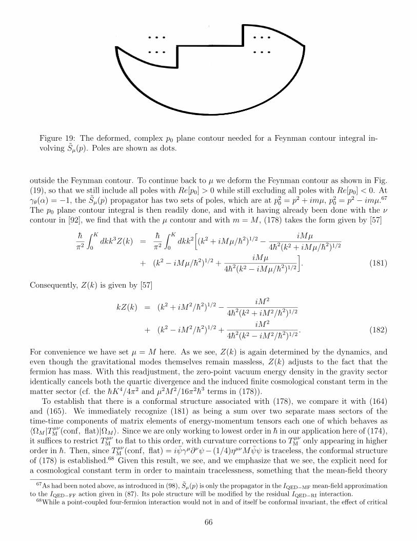
Figure 19: The deformed, complex p0 plane contour needed for a Feynman contour integral in-volving Sµ(p). Poles are shown as dots.
outside the Feynman contour. To continue back to µ we deform the Feynman contour as shown in Fig.(19), so that we still include all poles with Re[p0] > 0 while still excluding all poles with Re[p0] < 0. Atγθ(α) = −1, the Sµ(p) propagator has two sets of poles, which are at p2
0 = p2 + imµ, p20 = p2 − imµ.67
The p0 plane contour integral is then readily done, and with it having already been done with the νcontour in [92], we find that with the µ contour and with m = M , (178) takes the form given by [57]
h
π2
∫ K
0dkk3Z(k) =
h
π2
∫ K
0dkk2
[(k2 + iMµ/h2)1/2 − iMµ
4h2(k2 + iMµ/h2)1/2
+ (k2 − iMµ/h2)1/2 +iMµ
4h2(k2 − iMµ/h2)1/2
]. (181)
Consequently, Z(k) is given by [57]
kZ(k) = (k2 + iM2/h2)1/2 − iM2
4h2(k2 + iM2/h2)1/2
+ (k2 − iM2/h2)1/2 +iM2
4h2(k2 − iM2/h2)1/2. (182)
For convenience we have set µ = M here. As we see, Z(k) is again determined by the dynamics, andeven though the gravitational modes themselves remain massless, Z(k) adjusts to the fact that thefermion has mass. With this readjustment, the zero-point vacuum energy density in the gravity sectoridentically cancels both the quartic divergence and the induced finite cosmological constant term in thematter sector (cf. the hK4/4π2 and µ2M2/16π2h3 terms in (178)).
To establish that there is a conformal structure associated with (178), we compare it with (164)and (165). We immediately recognize (181) as being a sum over two separate mass sectors of thetime-time components of matrix elements of energy-momentum tensors each one of which behaves as〈ΩM |T µνM (conf, flat)|ΩM〉. Since we are only working to lowest order in h in our application here of (174),it suffices to restrict T µνM to flat to this order, with curvature corrections to T µνM only appearing in higherorder in h. Then, since T µνM (conf, flat) = iψγµ∂νψ− (1/4)ηµνMψψ is traceless, the conformal structureof (178) is established.68 Given this result, we see, and we emphasize that we see, the explicit need fora cosmological constant term in order to maintain tracelessness, something that the mean-field theory
67As had been noted above, as introduced in (98), Sµ(p) is only the propagator in the IQED−MF mean-field approximationto the IQED−FF action given in (87). Its pole structure will be modified by the residual IQED−RI interaction.
68While a point-coupled four-fermion interaction would not in and of itself be conformal invariant, the effect of critical
66

provides in the form of the −m2/2g term. Thus not only do we need to couple a critical scaling QED toa four-fermion interaction in order to cancel the logarithmic divergence in the vacuum energy density,this same coupling generates a cosmological constant term that serves to maintain conformal invariance.Moreover, not only does conformal invariance forbid the presence of any cosmological constant term inthe fundamental action, this same conformal invariance also controls the cosmological constant termthat is induced by the symmetry breaking. Since the residual interaction associated with the four-fermion interaction then generates dynamical Goldstone and Higgs bosons, we see that critical scaling,conformal symmetry, four-fermion interactions, dynamical Goldstone and Higgs boson generation, andcontrol of the cosmological constant are all intimately tied together.
Now all of the above cancellations occur no matter how big the µ2M2 ≡ M4 term in (178) mightbe (even if M is of Higgs mass scale, grandunified scale, or Planck scale), and none of it is observablesince the cancellations all occur in the vacuum, i.e. they are due entirely to the occupied negativeenergy states in the Dirac sea. However, what one measures in actual astrophysical phenomena is notproperties of the vacuum but the behavior of the positive energy modes that can be excited out of it. Tobe more precise, we note that since all of the infinities in T µνGRAV and T µνM are due to the infinite number ofmodes in the vacuum sector, if we decompose T µνGRAV and T µνM into finite particle (PART) and divergentvacuum (VAC) parts according to T µνGRAV = (T µνGRAV)PART + (T µνGRAV)VAC, T µνM = (T µνM )PART + (T µνM )VAC,(174) will decompose into
(T µνGRAV)VAC + (T µνM )VAC = 0, (183)
and
(T µνGRAV)PART + (T µνM )PART = 0. (184)
All of the vacuum energy density infinities and even the finite part in (178) are taken care of by (183),and for astrophysics and cosmology we can then use the completely infinity-free (184). In this way forstudying white dwarfs or the cosmic microwave background we can now use H =
∑a†(k)a(k)hωk alone
after all, as the zero-point contribution has already been taken care of by gravity itself and does notappear in (184) at all. Moreover, when we do excite positive energy modes out of the vacuum we willgenerate a new cosmological constant contribution, and it is this term that is measured in cosmology.Cosmology thus only sees the change in the vacuum energy density due to adding in positive energymodes and does not see the full negative energy mode vacuum energy density itself, i.e. in (184)one is sensitive not to 〈ΩM |T µνM |ΩM〉, and not even to 〈ΩM |bT µνM b†|ΩM〉, but only to their difference〈ΩM |bT µνM b†|ΩM〉 − 〈ΩM |T µνM |ΩM〉. Also gravity sees this effect mode by mode, i.e. gravity mode byfermion mode. Thus, for instance, in the application of TM
µν(conf) of (163) to cosmology that wasdescribed in [93] and is briefly discussed below, the quantity S0 is not 〈ΩM |S|ΩM〉 but the much smaller〈ΩM |bSb†|ΩM〉 − 〈ΩM |S|ΩM〉. In contrast, if one uses the Einstein gravity (168) and the matter fieldsource given in (157), then gravity sees an entire sum over fermion modes and sees the full and large〈ΩM |S|ΩM〉. To summarize, if one wants to take care of the cosmological constant problem, one hasto take care of the zero-point problem, and when one has a renormalizable theory of gravity, via aninterplay with gravity itself one is then able to do so.
scaling is to the spread out the four-fermion vertex. According to (90) for a given dθ the vertex would be spread out togive a non-local (NL) action of the form I(NL) =
∫d4xd4x′ψ(x)ψ(x)[(x−x′)2]−dθ ψ(x′)ψ(x′). With ψψ having dynamical
dimension dθ, under a conformal transformation I(NL) would transform into I(NL) =∫d4xd4x′e2αdθ ψ(eαx)ψ(eαx)[(x−
x′)2]−dθ ψ(eαx′)ψ(eαx′), and thus under a change of variable into I(NL) =∫d4yd4y′e−8αe2αdθe2αdθ ψ(y)ψ(y)[(y −
y′)2]−dθ ψ(y′)ψ(y′). Consequently, I(NL) is conformal invariant when dθ = 2, just as desired. Thus the non-local ac-tion
∫d4x
[−(1/4)FµνF
µν + ψγµ(i∂µ − eAµ)ψ]− (g/2)I(NL) is conformal invariant, as is its curved space generalization.
We can thus discuss the problem from the perspective of the standard local mean-field approach used in (87) and (88)or from the perspective of the non-local I(NL). When dθ = 2 the two approaches are equivalent, with the decompositioninto two separate mass sectors as exhibited in (181) allowing us to treat the vacuum energy density of one non-localtheory as that of two local ones.
67

11 Some Other Aspects of Conformal Symmetry and Confor-
mal Gravity
11.1 Conformal gravity and the Dark Matter Problem
With conformal symmetry as realized via critical scaling and anomalous dimensions being able toaddress some key issues in contemporary physics such as the generation of dynamical Goldstone andHiggs bosons, control of the cosmological constant, and the construction of a consistent quantum theoryof gravity, viz. conformal gravity, it is of interest to see how conformal gravity fares in addressing someother issues of concern to contemporary physics. In two recent papers [93, 92] the case was presentedfor considering conformal gravity as a possible alternative to standard Einstein gravity. In this sectionwe provide a brief update.
We had noted earlier that conformal invariance excludes the Einstein-Hilbert action. However, itdoes not exclude the Schwarzschild solution to Einstein gravity, since Rµν = 0 is an exact exteriorsolution to (173) in any source-free region where T µνM = 0.69 Moreover, to recover the successful resultsof a given theory one does not need to recover its equations, one only needs to recover its solutions, andone actually only needs to recover them in the kinematic region where they have been tested. However,while the Schwarzschild solution is a solution to conformal gravity, there are other solutions since thevanishing of W µν can be achieved without the vanishing of the Ricci tensor itself.
To determine what these other solutions might look like, Mannheim and Kazanas studied the ge-ometry associated with a static, spherically symmetric source in the conformal gravity theory, to find[108, 109] that the coefficient B(r) = −g00(r) obeyed the exact, all-order classical fourth-order Poissonequation
∇4B(r) =3
4αgB(r)(T 0
0 − T rr) = f(r). (185)
The general solution to this equation is given by
B(r) = −r2
∫ r
0dr′r′2f(r′)− 1
6r
∫ r
0dr′r′4f(r′)
−1
2
∫ ∞r
dr′r′3f(r′)− r2
6
∫ ∞r
dr′r′f(r′) +B0(r), (186)
where B0(r) obeys ∇4B0(r) = 0. Since the integration in (186) extends all the way to r = ∞, theB(r) potential receives contributions from material both inside and outside any system of interest.According to (186), matter confined to the interior of a star of radius r0 produces a potential exteriorto the star of the form V ∗(r > r0) = −β∗c2/r + γ∗c2r/2 per unit solar mass of star. We thus recoverthe Newtonian potential, while showing that in principle it does not need to be associated with thestandard Einstein gravitational theory.70 However, we find that the potential gets modified at largedistances where r = O[(β∗/γ∗)1/2], so that the solution recovers the Newton potential at short distancesonly, with the non-Ricci-flat solutions to conformal gravity only modifying the Ricci-flat one at largedistances and not at small ones. We thus recover the solution to Einstein gravity in the kinematic solarsystem region where it has been tested with the use of known luminous sources alone, while for an
69The Schwarzschild solution is not Riemann flat but only Ricci flat. However, even though the Weyl tensor doesdepend on the Riemann tensor, because of the Gauss-Bonnet theorem the conformal gravity action IW only depends onthe Ricci tensor and Ricci scalar as per (171). The variation Wµν of IW as given in (172) thus only depends on the Riccitensor and Ricci scalar and their derivatives, and all the terms in Wµν vanish identically if Rµν vanishes identically.
70While the solution given by (186) limits to the exterior Schwarzschild solution for small r, there is no limit in whichWµν becomes Rµν − (1/2)gµνRαα. We thus recover the standard model solution but do not recover its equations, withEinstein gravity only being sufficient to give the Schwarzschild solution and Newton’s Law of Gravity but not necessary.
68

appropriate galactic-determined value for γ∗, the solution will depart from Newton on precisely thosegalactic distances where in standard gravity one first has to resort to dark matter.
Specifically, for galaxies, integrating the V ∗(r) potential over a thin disk of stars with a surfacebrightness Σ(R) = Σ0 exp(−R/R0) with scale length R0 (the typical configuration for the stars in aspiral galaxy) yields the net local potential produced by the stars in the galaxy itself, and leads to alocally generated contribution to galactic circular velocities of the form [93]
v2LOC =
N∗β∗c2R2
2R30
[I0
(R
2R0
)K0
(R
2R0
)− I1
(R
2R0
)K1
(R
2R0
) ]
+N∗γ∗c2R2
2R0
I1
(R
2R0
)K1
(R
2R0
), (187)
where N∗ is the number of stars in the galaxy.There are two contributions due to material outside the galaxy, i.e. due to the rest of the universe.
The first contribution is a linear potential term with coefficient γ0/2 = (−k)1/2 coming from cosmology[93], a term that is associated with the B0(r) term, and due to writing a comoving Robertson-Walkergeometry with negative curvature in the rest frame coordinate system of the galaxy (with k > 0, γ0
would be complex). The second contribution arises from the integral from r to ∞ term in (186) dueto cosmological inhomogeneities such as clusters of galaxies, and is of a quadratic potential form withcoefficient κ [110]. Since both of these external contributions come from the universe as a whole, theyare both independent of any particular galaxy of interest, and thus act universally on every galaxy, withevery galaxy seeing the same γ0-dependent and κ-dependent potentials. When all these internal andexternal contributions are combined, the total rotational velocities in galaxies are given by
v2TOT = v2
LOC +γ0c
2R
2− κc2R2. (188)
When the present author first studied rotation velocity curves in the conformal gravity theory, thedata that were available did not go out far enough in distance for the −κc2R2 term to be significant,with the v2
TOT = v2LOC + γ0c
2R/2 formula providing a very good fit (see e.g. [93]) to a then available11 galaxy sample without the need for any dark matter. However, with 141 spiral galaxies now beingavailable and with 21 of them going out far enough in distance to be sensitive to the −κc2R2 term,Mannheim and O’Brien [110, 111, 112, 113] applied the full v2
TOT = v2LOC + γ0c
2R/2 − κc2R2 formulato the set of 141 rotation curves, and found very good fitting with parameters
β∗ = 1.48× 105cm, γ∗ = 5.42× 10−41cm−1,
γ0 = 3.06× 10⁻³⁰cm−1, κ = 9.54× 10−54cm−2, (189)
with no dark matter being needed. With (β∗/γ∗)1/2 being found to be of order 1023 cm, we see that theeffect of the linear γ∗ potential does indeed only become significant on galactic distance scales, as dothe γ0 and κ terms also. Consequently, without our requiring it a priori, solar system phenomenologyis left intact.
Even though there is only one free parameter per galaxy, viz. N∗, a parameter that is common toall galactic rotation curve fits, and even though there is basically no flexibility, (188) fully captures theessence of the data. Without the quadratic −κc2R2 term, the linear potential would eventually start todominate over the Newtonian potential and the typically flat galactic rotation curves would be expectedto begin to rise. However, no rise was found in the 21 galaxies in the 141 galaxy sample that went outthe furthest in distance, with each one possessing 10 or so points where a rise should have been seen.That these 200 or so points were then controlled by one single quadratic term with a universal coefficientthat acted on every single one of the 21 galaxies in exactly the same way is quite remarkable since one
69
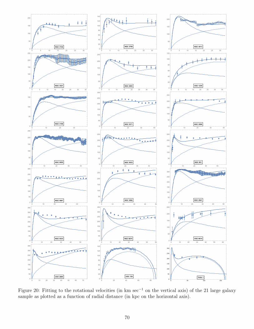
0 5 10 15 20 25 300
50
100
150
200
NGC 3726
0 5 10 15 20 25 300
20
40
60
80
100
120
140
NGC 3769
0 5 10 15 20 25 300
50
100
150
200
NGC 4013
0 5 10 15 20 25 30 350
50
100
150
200
250
NGC 3521
0 5 10 15 20 25 30 350
50
100
150
200
250
NGC 2683
0 5 10 15 20 25 30 350
20
40
60
80
100
120
UGC 1230
0 10 20 300
50
100
150
NGC 3198
0 10 20 30 400
50
100
150
200
250
300
NGC 5371
0 10 20 30 400
50
100
150
200
250
NGC 2998
0 10 20 30 400
50
100
150
200
250
NGC 5055
0 10 20 30 400
50
100
150
200
250
NGC 5033
0 10 20 30 400
50
100
150
200
250
NGC 801
0 10 20 30 400
50
100
150
200
250
300
NGC 5907
0 10 20 30 40 500
50
100
150
200
250
NGC 3992
0 10 20 30 40 500
50
100
150
200
250
300
NGC 2841
0 10 20 30 40 500
50
100
150
200
250
300
350
NGC 5533
0 10 20 30 40 50 600
50
100
150
200
250
300
350
NGC 6674
0 10 20 30 40 50 600
50
100
150
200
250
UGC 6614
0 10 20 30 40 50 60 700
50
100
150
200
250
300
350
UGC 2885
0 20 40 60 800
20
40
60
80
100
120
140
UGC 128
Figure 20: Fitting to the rotational velocities (in km sec−1 on the vertical axis) of the 21 large galaxysample as plotted as a function of radial distance (in kpc on the horizontal axis).
70

single parameter accounted for no less than 200 or so data points.71 For comparison, dark matter fits togalactic rotation curves typically require two free parameters per galactic dark matter halo (in additionto an N∗ for each galaxy), to thus need 282 more free parameters than the conformal theory in orderto fit the 141 galaxy sample. If dark matter is to be correct, then dark matter theory should be able toderive (188) as it does describe the galactic data. For the moment though there is no indication thatit can do so, or that it can predict the needed 282 halo parameters from first principles and show thatthey have any kind of universal relationship such as the one exhibited in (188). Moreover, there is alsono indication that supersymmetry, the most favored dark matter option, can do so either.72
As a final comment on the conformal gravity fitting to galactic rotation curves, we note that aswe go to even larger galactic distances than available in the current 141 galaxy sample, the quadratic−κc2R2 term will eventually start to dominate and galactic rotation curves must then start to fall.Moreover, since v2
TOT can never be negative, there would have to be a largest radial distance beyondwhich there would be no bound orbits.73 There would thus have to be a universal largest size thatgalaxies could be, of order γ0/κ ∼ 1023 cm, with the global physics that generates the γ0 and κpotential terms thus imposing a natural limit on the size of galaxies. Beyond the testable predictionthat galactic rotation curves must eventually start to fall, it is of interest to note that, in contrast to the1/r Newtonian potential where there is no upper limit to the possible size of bound orbits, in conformalgravity galactic orbits could not be of indefinitely large radius.
Now while much more still needs to be done in conformal gravity (a full list of the challenges thatconformal gravity currently faces may be found in [107]), two of the most urgent issues are gravita-tional lensing and fluctuations in the cosmic microwave background. For lensing the impact of therecently identified κ term needs to be worked out since one is dealing with light coming in from a non-asymptotically flat background. For fluctuations in the cosmic microwave background a first step hasrecently been taken with a conformal cosmology fluctuation theory having been presented in [107]. Itwould be of interest to ascertain whether conformal gravity could account for lensing or the temperaturevariations detected in the cosmic microwave background without any need for dark matter.
Also of cosmological interest is to note that through use of the conformal invariant matter actionIM(conf) given in (159),74 one can show that the Hubble plot associated with a conformal backgroundRobertson-Walker cosmology is described by a luminosity function dL(z) of the form [93]
dL(z) = − c
H0
(1 + z)2
q0
1−[1 + q0 −
q0
(1 + z)2
]1/2 , (190)
where z is the redshift, and where H0 and q0 are the current era values of the Hubble and decelerationparameters. On taking the parameter λ in IM(conf) to be negative (as required if IM(conf) is to beassociated with a cosmological phase transition in which the free energy is lowered), and on takingthe Robertson-Walker spatial three curvature k to be negative (as per the discussion above), in theconformal theory the structure of the cosmological evolution equations is such that q0 is constrained tolie in the interval −1 ≤ q0 ≤ 0 no matter what the magnitudes of the parameters in IM(conf). Fits
71Fits to the 21 largest galaxies are shown in Fig. (20). For each galaxy we exhibit the contributions due to theluminous Newtonian term alone (dashed curve), the two linear terms and the quadratic terms combined (dotted curve),with the full curve showing the total contribution. No dark matter is assumed.
72The success of any alternate theory of gravity in fitting astrophysical data cannot in and of itself exclude the possibleexistence of dark matter per se, with supersymmetry (whose existence is not in and of itself excluded by conformal gravity)for instance providing some potential dark matter candidates. However, the conformal gravity fits to galactic rotationcurves completely account for all the rotation curve data, to thus leave little room for any dark matter contribution thatmight appear alongside the conformal gravity contribution.
73In Fig. (20) we exhibit this effect for the two largest galaxies in the sample, UGC 128 and Malin 1.74As per the discussion of (184), the scalar field S in IM(conf) is to be understood as an expectation value over positive
frequency modes alone, viz. S = 〈ΩM |bψψb†|ΩM 〉 − 〈ΩM |ψψ|ΩM 〉, an altogether smaller quantity than 〈ΩM |ψψ|ΩM 〉itself.
71
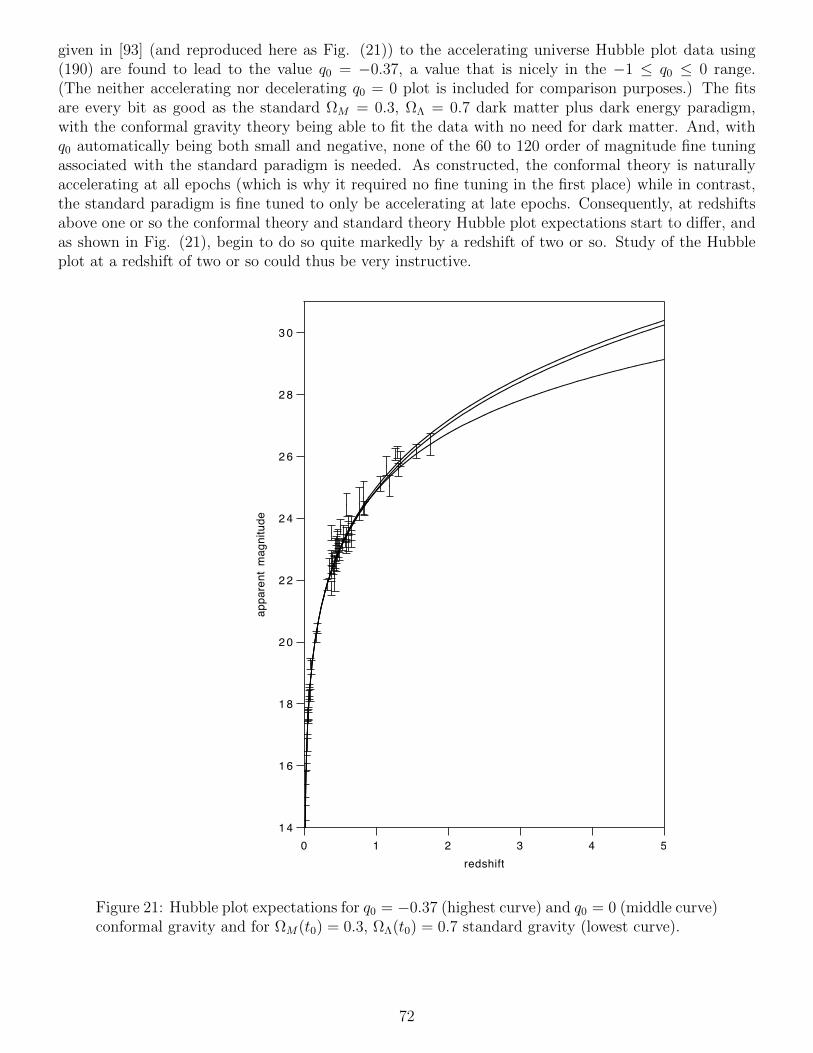
given in [93] (and reproduced here as Fig. (21)) to the accelerating universe Hubble plot data using(190) are found to lead to the value q0 = −0.37, a value that is nicely in the −1 ≤ q0 ≤ 0 range.(The neither accelerating nor decelerating q0 = 0 plot is included for comparison purposes.) The fitsare every bit as good as the standard ΩM = 0.3, ΩΛ = 0.7 dark matter plus dark energy paradigm,with the conformal gravity theory being able to fit the data with no need for dark matter. And, withq0 automatically being both small and negative, none of the 60 to 120 order of magnitude fine tuningassociated with the standard paradigm is needed. As constructed, the conformal theory is naturallyaccelerating at all epochs (which is why it required no fine tuning in the first place) while in contrast,the standard paradigm is fine tuned to only be accelerating at late epochs. Consequently, at redshiftsabove one or so the conformal theory and standard theory Hubble plot expectations start to differ, andas shown in Fig. (21), begin to do so quite markedly by a redshift of two or so. Study of the Hubbleplot at a redshift of two or so could thus be very instructive.
3 0
2 8
2 6
2 4
2 2
2 0
1 8
1 6
1 4
appa
rent
mag
nitu
de
543210redshift
Figure 21: Hubble plot expectations for q0 = −0.37 (highest curve) and q0 = 0 (middle curve)conformal gravity and for ΩM(t0) = 0.3, ΩΛ(t0) = 0.7 standard gravity (lowest curve).
72

11.2 Conformal Invariance and the Metrication of Electromagnetism
Another recent development in conformal gravity has been a study [114, 115] of a metrication of thefundamental forces, the very same objective that originally led Weyl to conformal symmetry in the firstplace. Just two years after Einstein metricated gravity with his development of general relativity, Weyl[102] attempted to metricate electromagnetism by proposing that the standard Riemannian geometryLevi-Civita connection
Λλµν =
1
2gλα(∂µgνα + ∂νgµα − ∂αgνµ) (191)
be augmented with a second connection, the Weyl connection
W λµν = −gλα(gναAµ + gµαAν − gνµAα) (192)
that expressly depended on the electromagnetic potential Aµ, to thus put Aµ into the geometry. Withthis augmentation, the generalized connection
Γλµν = Λλµν +W λ
µν (193)
has the remarkable property of being left invariant under a joint local transformation on the metric andthe electromagnetic potential of the form
gµν(x)→ e2β(x)gµν(x), Aµ(x)→ Aµ(x) + ∂µβ(x), (194)
for any spacetime-dependent β(x). Consequently, a generalized Riemann tensor or a generalized Weyltensor built out of this generalized connection would be invariant under (194) also. However, withthe covariant derivative of the metric associated with this generalized connection being the non-zero∇σg
µν = −2gµνAσ, parallel transport is then path (and thus history) dependent, with the theory thusbeing untenable.
Much later it was realized that the theory had another drawback. When W λµν is inserted into the
generalized Dirac action
ID =1
2
∫d4x(−g)1/2iψγcV µ
c (x)(∂µ + Γµ)ψ + H. c., (195)
where Γµ(x) = −(1/8)[γa, γb](Vbν ∂µV
aν +V bλ ΓλνµV
aν) is constructed with the generalized Γλµν connectiongiven in (193), the Weyl connection is found to drop out identically [116, 114]. Thus the Weyl connectionnever could have provided a geometric description of electromagnetism in the first place.
To rectify this, we note that the Weyl prescription for constructing Γλµν is to replace the ∂µ factorin Λλ
µν by ∂µ − 2Aµ. However, we recall that to obtain the standard minimal electromagnetic gaugecoupling we must use not ∂µ − Aµ but ∂µ − iAµ, with the factor of i actually being required becauseof Hermiticity or CPT invariance. Thus it is suggested [114] to proceed analogously with the Weylconnection by replacing W λ
µν by
V λµν = −2i
3gλα(gναAµ + gµαAν − gνµAα). (196)
Then, on using the generalized connection
Γλµν = Λλµν + V λ
µν (197)
in a generalized spin connection Γµ that is determined from it, following some algebra we find that thegeneralized Dirac action takes none other than the form [114]
ID =∫d4x(−g)1/2iψγcV µ
c (x)(∂µ + Γµ − iAµ)ψ (198)
73
With the action given in (198) being the standard one that is obtained by standard local electromagneticgauge invariance (viz. invariance under ψ(x)→ eiα(x)ψ(x), Aµ(x)→ Aµ(x) + ∂µα(x)), the metricationof electromagnetism is thereby achieved. The ID action thus has a dual characterization – it can begenerated via local gauge invariance or via a generalized geometric connection. The two viewpoints areequivalent.
As constructed, the action ID is not just locally gauge invariant, it is locally conformal invarianttoo, as it is left invariant under
ψ(x)→ e−3β(x)/2ψ(x), gµν(x)→ e2β(x)gµν(x), V aµ (x)→ eβ(x)V a
µ (x), Aµ(x)→ Aµ(x). (199)
However, comparing with (194), we see that in (199), this time Aµ(x) is not to transform at all. Inconsequence, neither a generalized Riemann tensor or a generalized Weyl tensor built out of the con-nection given in (197) would be invariant under (199). Moreover, neither would the standard Riemanntensor as constructed via the standard Levi-Civita connection alone be invariant either. However, theconformal Weyl tensor as constructed in (169) via the standard Levi-Civita connection alone would belocally conformal invariant under (199). Consequently, given the local conformal invariance that theDirac action possesses, the only action that we could write down in the pure gravity sector that wouldhave this invariance too would be the IW action given in (171). We are thus naturally led to conformalgravity. And since conformal gravity is based on a strictly Riemannian geometry with the standardLevi-Civita connection, there is no parallel transport problem, any more than there would have been ifwe had introduced Aµ into the Dirac action and obtained (198) by local electromagnetic gauge invari-ance in a theory with a Levi-Civita based Γµ. If (198) is associated with a strictly Riemannian geometrywhen Aµ is introduced via local electromagnetic gauge invariance, it must equally be associated witha strictly Riemannian geometry when Aµ is introduced via the generalized connection given in (197).Invariance under (199) thus forces the gravity sector to be strictly Riemannian, and there is no paralleltransport problem. The local conformal structure of ID thus prevents V λ
µν with its otherwise seeminglyproblematic factor of i from coupling in the gravity sector, to thereby render the gravity sector real.And, with there being no parallel transport problem, even with its non-zero V λ
µν , the theory is viable.
11.3 Conformal Gravity and the Metrication of the Fundamental Forces
To generalize metrication to incorporate axial symmetry, we allow for torsion and introduce the anti-symmetric Cartan torsion tensor Qλ
µν and the associated contorsion Kλµν according to
Qλµν = Γλµν − Γλνµ = −Qλ
νµ, Kλµν =
1
2gλα(Qµνα +Qνµα −Qανµ). (200)
Then with
Sµ =1
8(−g)−1/2εµαβγQαβγ, (201)
insertion of
Γλµν = Λλµν + V λ
µν +Kλµν (202)
into Γµ is found [117] to change ID of (198) into
ID =∫d4x(−g)1/2iψγcV µ
c (x)(∂µ + Γµ − iAµ − iγ5Sµ)ψ. (203)
This action is invariant under ψ(x) → exp[iγ5δ(x)]ψ(x), Sµ(x) → Sµ(x) + ∂µδ(x), with local axialsymmetry thus being metricated too. The action is also invariant under local conformal transformations
74
as well, if, just like Aµ(x), Sµ(x) does not transform under a local conformal transformation at all (viz.Sµ(x) → Sµ(x)). It is our view that rather than being something arcane, torsion manifests itself asan axial gauge boson, one that would then have escaped detection if it acquires a large enough Higgsmechanism mass. Thus if we seek a metrication of the fundamental forces through the Weyl and torsionconnections, we are led to a quite far reaching conclusion: not only must the fundamental forces bedescribed by local gauge theories, they must be described by spontaneously broken ones.
The extension to the non-Abelian case is also direct. If for instance we put the fermions into thefundamental representation of SU(N)×SU(N) with SU(N) generators T i that obey [T i, T j] = if ijkT k,replace Aµ by gV T
iAiµ, replace Qαβγ by gATiQi
αβγ, and thus replace Sµ by gATiSiµ in the connections,
we obtain a locally SU(N)× SU(N) invariant Dirac action of the form [114, 57]
JD =∫d4x(−g)1/2iψγcV µ
c (∂µ + Γµ − igV T iAiµ − igAγ5T iSiµ)ψ. (204)
We can thus metricate chirally-symmetric non-Abelian theories (on setting gA = gV ). As constructed,the action JD is quite remarkable, as it not only possesses some of the key local invariances in physics, viz.general coordinate invariance, local Lorentz invariance, local vector non-Abelian gauge symmetry, localaxial-vector non-Abelian gauge symmetry, and local conformal symmetry, every one of these invariancescan have a geometric origin.
11.4 The Inevitability of Conformal Gravity
When the fermion spin connection Γµ(x) was first introduced into physics, its purpose was to imple-ment local Lorentz invariance, since while iψγµ∂µψ was invariant under global Lorentz transforma-tions on ψ of the form ψ → exp(iwµνMµν)ψ with a spacetime-independent wµν , on its own iψγµ∂µψwas not invariant under local ones in which wµν depended on the spacetime coordinates. However,iψγcV µ
c (x)(∂µ + Γµ)ψ is. Now while it was not intended, the standard curved space massless Diracaction
∫d4x(−g)1/2iψγcV µ
c (x)(∂µ + Γµ)ψ with a Levi-Civita based spin connection just happens to beinvariant under the local conformal transformations given in (199).75 Thus, as we see, we are essen-tially getting local conformal invariance for free, without needing to ask for it a priori. Moreover, wecan interpret Γµ(x) as the gauge field of local conformal invariance in exactly the same way as Aµ(x)acts as the gauge field of local gauge invariance, with both the real and the imaginary parts of the−3β/2 + iα phase of the fermion being gauged. Now while the conformal invariance of the masslessDirac action would be lost if the fermion were to be massive, in order to maintain conformal invarianceat the level of the Lagrangian we would need mass to be induced dynamically, precisely just as wehave been considering in this article. With the same analysis holding for all of the fundamental strong,electromagnetic, and weak interactions since they are all based on local gauge theories with dimension-less coupling constants, they would all be fully conformal invariant at the level of the Lagrangian ifall masses are induced dynamically. We thus see that if there are no fundamental mass terms at alland if all mass is to come from vacuum breaking, conformal invariance is a quite natural invariance forphysics.76 In this way we see an intimate connection between conformal symmetry and dynamical massgeneration.
Further support for the relevance of conformal gravity may be found by doing a fermionic pathintegration of the Dirac action given in (204). If we set
∫D[ψ]D[ψ] exp(iJD) = exp(iIEFF), then with
75In flat spacetime the action∫d4xiψγµ∂µψ is invariant under the global ψ(xµ) → e−3β/2ψ(eβxµ), as the change of
variable x′µ = eβxµ reveals. The spin connection is then needed when β is taken to depend on the spacetime coordinates.76In the standard SU(2) × U(1) theory of electroweak interactions, there is just one fundamental mass scale in the
Lagrangian, namely that associated with the µ2φ2/2 term in the Lagrangian of an elementary Higgs field. In a criticalscaling theory with a dynamical Higgs field, such non-conformal-invariant terms do not appear in the fundamentalLagrangian.
75

JD being linear in both ψ and ψ the fermion path integral can be done analytically. On doing thefermion path integration we generate an effective action IEFF whose leading term is of the form
IEFF =∫d4x(−g)1/2C
[1
20
[RµνR
µν − 1
3(Rα
α)2]
+1
3GiµνG
µνi +
1
3SiµνS
µνi
], (205)
where C is a log divergent constant, and Gµνi and Sµνi are the standard non-Abelian antisymmetric rank
two tensors associated with Aiµ and Siµ.77 We recognize the terms in (205) as respectively being of theform of none other than the bosonic gµν , A
iµ, and Siµ sectors of the conformal gravity, vector Yang-Mills,
and axial-vector Yang-Mills theories. That IEFF must have the form that it has is because it mustpossess all the local symmetries that JD itself possesses. As we see, the Λλ
µν , Vλµν , and Kλ
µν contributions
to the generalized Γµ lead to three distinct and independent sectors in (205), and despite the pres-ence of non-Abelian terms in Γµ, the resulting conformal gravitational sector expressly has no internalsymmetry dependence, just as one would want. Thus save only for the gravity sector, we recognize(204) and (205) as the standard action used in fundamental physics, only now all generated geomet-rically. Geometry and conformal invariance thus lead us to (204) and (205), in exactly the same wayas conformal invariance and gauge invariance would also do. We note that we do not induce either theEinstein-Hilbert IEH = −(1/16πG)
∫d4x(−g)1/2Rα
α or the cosmological constant IΛ = −∫d4x(−g)1/2Λ
actions as neither action is conformal invariant (G and Λ both carry dimension). Rather, we expresslyinduce IW, and in fact cannot avoid doing so. In [92] we have made the case for local conformal gravity,while in [121] ’t Hooft has made the case for local conformal symmetry, with ’t Hooft even noting [122]that a conformal structure for gravity seems to be inevitable, just as we find here.
To explicitly see how the conformal structure is maintained in the presence of mass, we note that if wedo introduce a mass term into the action and augment JD with δJD = −
∫d4x(−g)1/2M(x)ψ(x)ψ(x),
then IEFF is modified to IEFF + δIEFF, with the fermion path integration yielding (ignoring internalsymmetry indices) [118, 92]
δIEFF =∫d4x(−g)1/2C
[−M4(x) +
1
6M2(x)Rα
α
− (∂µ + iAµ + iγ5Sµ)M(x)(∂µ − iAµ − iγ5Sµ)M(x)]. (206)
Comparing with (159), we see that we have naturally generated an M(x) dependence that throughthe M2(x)Rα
α/6 term is conformally coupled to the geometry, just as must be the case since in thefermion path integration the δJD mass term acts in the same locally conformal invariant manner as aYukawa-coupled scalar field. Now while we have generated IEFF and δIEFF by doing a path integrationover the fermions, this is equivalent to doing a one fermion loop Feynman diagram calculation. Onnow comparing with the one-loop mean-field IEFF given in (62) and (63), we recognize (206) as beingequivalent to the mean-field action when we evaluate (62) at the energy density minimum where m(x) =M , as then generalized to curved space. On dressing the point fermion loop diagrams with photonexchange dressings (i.e. on additionally doing a path integration of exp(iJD) over Aµ), we see that ifwe have critical scaling and γθ(α) = −1, (206) will be dressed into (107), as appropriately generalized.Thus if mass is generated by a mean-field procedure in which there is a four-fermion interaction, themean field will precisely have the form given in (206), as then dressed by a critical scaling that makesthe four-fermion interaction be both power-counting renormalizable and conformal invariant. Below wediscuss the four-fermion interaction terms in more detail.
The very fact that fermion path integration generated the conformal gravity action in (205) reinforcesthe result of [90, 91] that conformal gravity is ghost free and unitary. Specifically, since the relevant
77The gµν-dependent and Aiµ-dependent components of IEFF and the value of the constant C may be found in [118,
119, 120] and the Siµ-dependent component may be found in [117].
76
fermion path integration is equivalent to a one loop Feynman diagram, and since one cannot change thestructure of a Hilbert space in perturbation theory, it must be the case that either JD and IEFF bothhave states of negative norm or neither does. But the JD action is the standard fermion sector actionthat is used in particle physics all the time, and it is completely free of states with negative norm. Thusconformal gravity must be free of negative norm states also,78 and must thus be as consistent at thequantum level as the JD action from which it can be derived.
11.5 A Theory of Everything
Since there is a log divergence in (205), and since (205) is obtained via a fermion loop radiative correction,we can cancel the divergence by a counterterm. To do so we augment the Dirac action JD with afundamental Yang-Mills gauge field (IYM) action and a conformal (IW) metric sector action of the form
IW + IYM =∫d4x(−g)1/2
[− 2αg
(RµνR
µν − 1
3(Rα
α)2)− 1
4GiµνG
µνi −
1
4SiµνS
µνi
]. (207)
Even while this action will now take care of the infinities in (205) and its higher order radiative correc-tions, there will still be uncanceled vacuum energy density contributions. To cancel them we introducean SU(N)× SU(N) invariant four-fermion action with coupling gFF, viz.
IFF = −∫d4x(−g)1/2 gFF
2
[ψT iψψT iψ + ψiγ5T iψψiγ5T iψ
], (208)
and can thus we write down a fundamental action for a conformal invariant universe, viz.
IUNIV = JD + IW + IYM + IFF, (209)
with there being no ψV iµψψV
µi ψ type four-fermion interactions as they have been replaced via the
introduction of intermediate vector bosons, vector bosons which themselves couple conformally. If thedynamics associated with (209) leads to an IFF with dynamical dimension equal to four, the IUNIV actionwill then provide a fully conformal invariant, renormalizable, and consistent action for the universe inwhich all mass is generated in the vacuum by dynamical symmetry breaking, with all bound states beinggenerated by the residual interaction associated with IFF.79 As regards the four-fermion IFF term, wenote that it makes the vacuum energy density finite when dθ = 2, while also making the four-fermioninteraction contribution to the scalar and pseudoscalar channel TS(q2,M) and TP(q2,M) scatteringamplitudes be finite too, just as discussed in Secs. (8.4) and (8.8). However, there are also gauge bosonand graviton contributions to scattering amplitudes, and the contributions that they make via IW +IYM
are also all renormalizable. Moreover, if the beta functions associated with all three of the conformalgravity, vector Yang-Mills, and axial-vector Yang-Mills actions all vanish, and if all the associated non-Abelian dθ are all equal to two, not only would the full IUNIV theory be renormalizable, the theorywould even be finite and exist without renormalization [57] [just as the Schwinger-Dyson equation andthe fermion-antifermion scattering amplitudes (cf. (73), (117), (126)) exist without renormalizationin the Abelian case]. Thus for weak interactions we make the four-fermion interaction model of weak
78As noted in [115], to establish unitarity in a conformal gravity path integral formulation requires continuing thepath integral measure into the complex plane, just as one always has to do [105] in non-Hermitian theories such asconformal gravity because of the need to obtain well-behaved asymptotic boundary conditions (cf. Sec. (10.4)), with sucha continuation being needed in order to enable the path integral to exist.
79While we have formally introduced IUNIV here, doing actual mass generation calculations that would yield quarkand lepton mass spectra is for the future. However, as our derivation of TP(q2,M) and TS(q2,M) in (117) and (126)shows, in the dynamical case the pseudoscalar and scalar bound state Yukawa couplings to fermion-antifermion pairs aredetermined by the dynamics and do not need to be taken as input parameters as in the elementary Higgs case. Thus inthe dynamical case the free parameters associated with the quark and lepton mass matrices are potentially calculable.
77

interactions renormalizable by replacing it by a gauge theory whose gauge bosons become massivethrough the Higgs mechanism, and in the presence of gravity we make the vacuum energy density finiteby introducing an IFF four-fermion interaction that is made renormalizable by anomalous dimensions.There are thus two ways to control the divergences of four-fermion interactions, either replace them bya gauge theory or soften them via anomalous dimensions, and both play a role in physics. Given itscontent, we can identify (209) as a candidate theory of everything, one that is potentially finite, andone that is formulated in the four spacetime dimensions for which there is evidence.80
12 Comparing Conformal Symmetry and Supersymmetry
It is of interest to compare conformal symmetry and supersymmetry, as they both seek to addressmany of the same issues. In order to compare them, we note first that unlike supersymmetry, conformalsymmetry does not need to be postulated. Specifically, if we start with fermions alone and couplethem to curved space via the requirement of local Lorentz invariance, we will directly be led to the∫d4x(−g)1/2iψγcV µ
c (x)(∂µ+Γµ)ψ action. As noted above, this action is not just locally Lorentz invariantbut is locally conformal invariant too. However, it is not in any way supersymmetric. Thus for the∫d4x(−g)1/2iψγcV µ
c (x)(∂µ + Γµ)ψ action local conformal invariance is output not input (as is then theconformal gravity action generated in (205) by fermion path integration), and thus never needs to bepostulated. However one cannot get from iψγcV µ
c (x)(∂µ + Γµ)ψ to a supersymmetric action withoutpostulating the existence of bosonic superpartners of the fermions. The reason why it is fermions andconformal symmetry rather than fermions, bosons and supersymmetry that is singled out is that the15-dimensional O(4, 2) conformal group is the full symmetry of the light cone on which all particlesmove in the absence of mass. And with the 15-dimensional SU(2, 2) being the covering group of theconformal group, the fundamental representation of the conformal group is the four-component spinor,all on its own with no bosonic superpartner being needed. Moreover, if all mass scales are to begenerated dynamically, there must be an underlying conformal symmetry in the fundamental action,with it only being broken in the vacuum.
In terms of what conformal symmetry and supersymmetry aspire to do, we note that both theoriesseek to address the vacuum energy density problem, the cosmological constant problem, the Higgs self-energy problem, the dark matter problem, and the quantum gravity problem. While supersymmetrycan address the first three of these problems when it is unbroken, as we had noted above, it runs intodifficulty once the supersymmetry is broken. While supersymmetry can provide possible dark mattercandidates, it is not yet able to derive a formula such as the observationally-tested conformal gravityformula given in (188) for galactic rotation curves, or provide a formula that requires no fine tuningfor the Hubble plot such as the conformal gravity one given in (190). And as to quantum gravity,to construct a consistent string theory of quantum gravity, one needs not just supersymmetry, one inaddition needs six extra spacetime dimensions. And then beyond all this, superparticles of course needto found, and yet to date there is no sign of any of them, either at the LHC or in underground darkmatter searches.
As we have seen in this article, for every one of these five major problems conformal symmetryappears to be doing better than supersymmetry, primarily because it is able to retain control of theseproblems even after the conformal symmetry is spontaneously broken. Through conformal symmetryone is able to resolve these problems without the need for any dark matter, any dark energy, or anyfine tuning of parameters. In addition, through conformal symmetry one can construct a consistent,unitary, and renormalizable theory of quantum gravity without any new particles or any extra spacetimedimensions. And one can do so while making some readily testable predictions such as the extension of
80Since string theory requires both supersymmetry and extra dimensions, if neither actually exists, then rather thanbeing a possible theory of everything, string theory would instead be a theory of more than everything.
78
(188) and (190) beyond the domains in which they have currently been tested. Determining whether theHiggs boson is elementary or dynamical could go a long way to establishing whether it is supersymmetry(as needed for the self-energy hierarchy problem of an elementary Higgs boson) or conformal symme-try (critical scaling, anomalous dimensions, a dynamically generated Higgs boson with no hierarchyproblem, and a renormalizable four-fermion interaction) that might be favored.81
13 Summary
In this article we have addressed the question of whether the Higgs boson is elementary or composite.Even though the standard elementary Higgs boson electroweak model works extremely well, there arenonetheless some basic concerns with the model: (i) radiative corrections to the Higgs self-energy havea high scale hierarchy problem, (ii) there is an enormous number of free parameters in the coupling ofthe Higgs boson to the quarks and leptons, (iii) in its spontaneously broken phase the Higgs potentialprovides a large contribution to the cosmological constant, (iv) as with any quantum field theory thereis a zero-point problem, though this only becomes of concern when the theory is coupled to gravity, as itultimately must be, and (v) the whole notion of an elementary Higgs boson stands in sharp contrast tothe BCS theory of superconductivity or the generation of a Goldstone boson pion in strong interactionssince neither of these two well-established cases involves any elementary Higgs boson at all, with thebreaking being done dynamically by fermion bilinear condensates. As we have shown, all of theseconcerns can be addressed if the symmetry breaking is dynamical: (i) a bound state Higgs boson hasno hierarchy problem, (ii) when the Higgs boson is a bound state, the same dynamics that fixes itsmass as the position of the pole in a fermion-antifermion scattering amplitude also fixes its couplingto the fermions as the residue at the pole, (iii,iv) when the Higgs generation mechanism involves thefour-fermion interaction then on coupling to conformal gravity one can resolve both the cosmologicalconstant problem and the zero-point problem, and (v) with a dynamical Higgs boson electroweak andstrong interaction symmetry breaking are treated equivalently.
14 The Moral of the Story
With the vacuum of quantum field theory being a dynamical one, in a sense Einstein’s ether hasreemerged. Only it has reemerged not as the mechanical ether of classical physics that was excludedby the Michelson-Morley experiment, but as a dynamical, quantum-field-theoretic one full of Dirac’snegative energy particles, an infinite number of such particles whose dynamics can spontaneously breaksymmetries. The type of physics that would be taking place in this vacuum depends on how symmetriesare broken, i.e. on whether the breaking is by elementary Higgs fields or by dynamical composites. Ifthe symmetry is broken by an elementary Higgs field, then the Higgs boson gives mass to fundamentalgauge bosons and fermions alike. However, if the breaking is done dynamically, then it is the structureof an ordered vacuum itself that generates masses, with the mass generation mechanism in turn thenproducing the Higgs boson. In the dynamical case then mass produces Higgs rather than Higgs producesmass. In the dynamical case we should not be thinking of the Higgs boson as being the “god particle”.
81While critical scaling and anomalous dimensions were key components of the conformal bootstrap program that wasdeveloped in the 1970s by workers such as Migdal and Polyakov, it is of interest to note that with the current focus onconformal field theories in the literature, the conformal bootstrap program has recently come into vogue again (for areview see e.g. [123]). Author’s note: it is also of interest to note that Robert Brout and Francois Englert were interested[124, 125] in the conformal bootstrap program when I was a post-doc with them in Brussels in the early seventies justat the time that condensed matter renormalization group ideas were coming into particle physics, and my own interestin JBW electrodynamics and also [126] in the conformal bootstrap was stimulated by my interaction with them at thattime.
79
Rather, if anything, we should be thinking of the vacuum as being the “god vacuum”.
15 Acknowledgments
The author wishes to thank Michael Mannheim, Brendan Pratt, and Candost Akkaya for help inpreparing the figures, and Drs. Joshua Erlich, Valery P. Gusynin, and Juha Javanainen for comments.
References
[1] F. Englert, R. Brout, Phys. Rev. Lett. 13 (1964) 321
[2] P.W. Higgs, Phys. Lett. 12 (1964) 132
[3] P.W. Higgs, Phys. Rev. Lett. 13 (1964) 508
[4] ATLAS Collaboration, G. Aad et. al., Phys. Lett. B 716 (2012) 1
[5] CMS Collaboration, S. Chatrchyan et. al., Phys. Lett. B 716 (2012) 30
[6] V.L. Ginzburg, L.D. Landau, Zh. Eksp. Teor. Fiz. 20 (1950) 1064
[7] J. Bardeen, L.N. Cooper, J.R. Schrieffer, Phys. Rev. 108 (1957) 1175
[8] L.P. Gorkov, Sov. Phys. JETP 9 (1959) 1364
[9] P.W. Anderson, Phys. Rev. 110 (1958) 827
[10] Y. Nambu, Phys. Rev. 117 (1960) 648
[11] Y. Nambu, Phys. Rev. Lett. 4 (1960) 380
[12] J. Goldstone, Nuovo Cimento 19 (1961) 154
[13] Y. Nambu, G. Jona-Lasinio, Phys. Rev. 122 (1961) 345
[14] J. Goldstone, A. Salam, S. Weinberg, Phys. Rev. 127 (1962) 965
[15] J. Schwinger, Phys. Rev. 125 (1962) 397
[16] J. Schwinger, Phys. Rev. 128 (1962) 2425
[17] P.W. Anderson, Phys. Rev. 130 (1963) 439
[18] A. Klein, B.W. Lee, Phys. Rev. Lett. 12 (1964) 266
[19] W. Gilbert, Phys. Rev. Lett. 12 (1964) 713
[20] G.S. Guralnik, C.R. Hagen, T.W.B. Kibble, Phys. Rev. Lett. 13 (1964) 585
[21] F. Close, The Infinity Puzzle: The Personalities, Politics, and Extraordinary Science Behind theHiggs Boson, Oxford University Press, Oxford, 2013
[22] G. Jona-Lasinio, Nuovo Cimento 34 (1964) 1790
[23] S. Coleman, E. Weinberg, Phys. Rev. D 7 (1973) 1888
[24] R. Brout, Phase Transitions, W. A. Benjamin, New York, 1965
[25] L.N. Cooper, Phys. Rev. 104 (1956) 1189
80
[26] P.D. Mannheim, Phys. Rev. D 12 (1975) 1772
[27] J.M. Cornwall, R. Jackiw, E. Tomboulis, Phys. Rev. D 10 (1974) 2428
[28] P.D. Mannheim, Phys. Rev. D 10 (1974) 3311
[29] P.D. Mannheim, Nucl. Phys. B 143 (1978) 285
[30] R. Fukuda, Prog. Theor. Phys. 78 (1987) 1487
[31] R. Fukuda, M. Komachiya, M. Ukita Phys. Rev. D 38 (1988) 3747
[32] V.A. Miransky, Dynamical Symmetry Breaking in Quantum Field Theories, World Scientific Pub-lishing Co., Singapore, 1993.
[33] W.A. Bardeen, M.S. Chanowitz, S.D. Drell, M. Weinstein, T.-M. Yan, Phys. Rev. D 11 (1975)1094
[34] T. Eguchi, H. Sugawara, Phys. Rev. D 10 (1974) 4257
[35] P.D. Mannheim, Phys. Rev. D 14 (1976) 2072
[36] R. Jackiw, K. Johnson, Phys. Rev. D 8 (1973) 2386
[37] J.M. Cornwall, R.E. Norton Phys. Rev. D 8 (1973) 3338
[38] K. Johnson, M. Baker, R. Willey, Phys. Rev. 136 (1964) B1111
[39] K. Johnson, R. Willey, M. Baker, Phys. Rev. 163 (1967) 1699
[40] M. Baker, K. Johnson, Phys. Rev. 183 (1969) 1292
[41] M. Baker, K. Johnson, Phys. Rev. D 3 (1971) 2516
[42] M. Baker, K. Johnson, Phys. Rev. D 3 (1971) 2541
[43] K. Johnson, M. Baker, Phys. Rev. D 8 (1973) 1110
[44] T. Maskawa, H. Nakajima, Prog. Theor. Phys. 52 (1974) 1326
[45] T. Maskawa, H. Nakajima, Prog. Theor. Phys. 54 (1975) 860
[46] R. Fukuda, T. Kugo, Nucl. Phys. B 117 (1976) 250
[47] P.I. Fomin, V.P. Gusynin, V.A. Miransky, Phys. Lett. B 78 (1978) 136
[48] K. Yamawaki, Int. J. Mod. Phys. A 25 (2010) 5128
[49] V.A. Miransky, Nuovo Cimento A 90 (1985) 149
[50] S.L. Adler, W.A. Bardeen, Phys. Rev. D 4 (1971) 3045 E: 6 (1972) 734
[51] S.L. Adler, Phys. Rev. D 5 (1972) 3021
[52] C.N. Leung, S.T. Love, W.A. Bardeen, Nucl. Phys. B 273 (1986) 649
[53] K. Yamawaki, M. Bando, K. Matumoto, Phys. Rev. Lett. 56 (1986) 1335
[54] S. Coleman, Comm. Math. Phys. 31 (1973) 259
[55] P. D. Mannheim, On the Absence of the Goldstone Mode in the Vector Gluon Model, LBL-3340,September 1974.
81

[56] K. Johnson, in Proceedings of the Ninth Latin American School of Physics I. Saavedra (Ed.)Benjamin, New York, 1968.
[57] P.D. Mannheim, Living Without Supersymmetry – the Conformal Alternative and a DynamicalHiggs Boson, arXiv:1506.01399 [hep-ph], June 2015
[58] P.D. Mannheim, Critical Scaling and a Dynamical Higgs Boson, arXiv:1604.07696 [hep-ph], April2016
[59] W.A. Bardeen, C.N. Leung, S.T. Love, Phys. Rev. Lett. 56 (1986) 1230
[60] K. Kondo, H. Mino, K. Yamawaki, Phys. Rev. D 39 (1989) 2430
[61] W.A. Bardeen, S.T. Love, V.A. Miransky, Phys. Rev. D 42 (1990) 3514
[62] W.A. Bardeen, S.T. Love, Phys. Rev. D 45 (1992) 4672
[63] M. Carena, C.E.M. Wagner, Phys. Lett. B 285 (1992) 277
[64] V.P. Gusynin, V.A. Miranskii, Zh. Eksp. Teor. Fiz. 101 (1992) 414
[65] K. Kondo, M. Tanabashi, K. Yamawaki, Prog. Theor. Phys. 89 (1993) 1249
[66] M. Harada, Y. Kikukawa, T. Kugo, H. Nakano, Prog. Theor. Phys. 92 (1994) 1161
[67] M. Hashimoto, Phys. Lett. B 441 (1998) 389
[68] V.P. Gusynin, M. Reenders, Phys. Rev. D 57 (1998) 6356
[69] T. A. Ryttov, R. Shrock, Phys. Rev. D 83 (2011) 056011
[70] B. Holdom, Phys. Rev. D 24 (1981) 1441
[71] V.A. Miransky, P.I. Fomin, Phys. Lett. B 105 (1981) 387
[72] B. Holdom, Phys. Lett. B 150 (1985) 301
[73] T. Appelquist, D. Karabali, L.C.R. Wijewardhana, Phys. Rev. Lett. 57 (1986) 957
[74] B. Holdom, Phys. Lett. B 198 (1987) 535
[75] T. Appelquist, J. Terning, L.C.R. Wijewardhana, Phys. Rev. D 44 (1991) 871
[76] T. Appelquist, Y. Bai, Phys. Rev. D 82 (2010) 071701
[77] C.T. Hill, E.H. Simmons, Phys. Rep. 381 (2003) 235 E: 390 (2004) 553
[78] V.A. Miransky, Int. J. Mod. Phys. A 25 (2010) 5105
[79] R. Contino, The Higgs as a Composite Nambu-Goldstone Boson, arXiv:1005.4269 [hep-ph], inPhysics of the Large and the Small, TASI 09, Proceedings of the Theoretical Advanced StudyInstitute in Elementary Particle Physics, Boulder, 2009. C. Csaki, S. Dodelson (Eds.), WorldScientific Publishing Co., Singapore 2011.
[80] T. Appelquist, Int. J. Mod. Phys. A 25 (2010) 5114
[81] G. Panico, A. Wulzer, The Composite Nambu-Goldstone Higgs, arXiv:1506.01961 [hep-ph], June2015.
[82] T. Appelquist, K. Lane, U. Mahanta, Phys. Rev. Lett. 61 (1988) 1553
[83] B. Holdom, Phys. Lett. B 213 (1988) 365
82
[84] B. Holdom, Phys. Rev. Lett. 62 (1989) 997
[85] U. Mahanta, Phys. Lett. B 225 (1989) 181
[86] V.A. Miransky, K. Yamawaki, Mod. Phys. Lett. A 4 (1989) 129
[87] P.D. Mannheim, Anomalous Dimensions and the Renormalizability of the Four-Fermion Interac-tion, arXiv:1611.09129 [hep-th], November 2016
[88] P.D. Mannheim, Phys. Rev. D 22 (1980) 1729
[89] P.D. Mannheim, Mod. Phys. Lett. A 26 (2011) 2375
[90] C.M. Bender, P.D. Mannheim, Phys. Rev. Lett. 100 (2008) 110402
[91] C.M. Bender, P.D. Mannheim, Phys. Rev. D 78 (2008) 025022
[92] P.D. Mannheim, Found. Phys. 42 (2012) 388
[93] P.D. Mannheim, Prog. Part. Nucl. Phys. 56 (2006) 340
[94] J. Wess, J. Bagger, Supersymmetry and Supergravity, Princeton Series in Physics, S. B. TreimanEd. (Princeton University Press, Princeton NJ, 1992).
[95] S. Weinberg, The Quantum Theory of Fields, Volume III: Supersymmetry, (Cambridge UniversityPress, Cambridge UK, 2000).
[96] J. Polchinski, String Theory, Volume II: Superstring Theory and Beyond, (Cambridge UniversityPress, Cambridge UK, 1998).
[97] M. Shifman, Frontiers Beyond the Standard Model: Reflections and Impressionistic Portrait ofthe Conference, FTPI, October 2012, arXiv:1211.0004 [physics.pop.ph].
[98] R. Aaij et. al. (LHCb Collaboration), Phys. Rev. Lett. 110 (2013) 021801
[99] V. Khachatryan et. al. (CMS and LHCb Collaborations), Nature 522 (2015) 68
[100] G.E. Volovik, Annalen. Physik 14 (2005) 165
[101] V. Branchina, D. Zappala, Mod. Phys. Lett. A 25 (2010) 2305
[102] H. Weyl, Sitzsungber. Preuss. Akad. Wiss. (1918) 465
[103] H. Weyl, Math. Zeit. 2 (1918) 384
[104] A. Pais and G.E. Uhlenbeck, Phys. Rev. 79 (1950) 145
[105] P.D. Mannheim, Antilinearity Rather than Hermiticity as a Guiding Principle for Quantum The-ory, arXiv:1512.04915 [hep-th], December 2015
[106] P.D. Mannheim, Phys. Lett. B 753 (2016) 288
[107] P.D. Mannheim, Phys. Rev. D 85 (2012) 124008
[108] P.D. Mannheim, D. Kazanas, Astrophys. J. 342 (1989) 635
[109] P.D. Mannheim, D. Kazanas, Gen. Rel. Gravit. 26 (1994) 337
[110] P.D. Mannheim, J.G. O’Brien, Phys. Rev. Lett. 106 (2011) 121101
[111] P.D. Mannheim, J.G. O’Brien, Phys. Rev. D 85 (2012) 124020
[112] J.G. O’Brien, P.D. Mannheim, Mon. Not. R. Astron. Soc. 421 (2012) 1273
83
[113] P.D. Mannheim, J.G. O’Brien, J. Phys. Conf. Ser. 437 (2013) 012002
[114] P.D. Mannheim, PT Symmetry, Conformal Symmetry, and the Metrication of Electromagnetism,arXiv:1407.1820 [hep-th], July 2014. Found. Phys., in press
[115] P.D. Mannheim, Int. Jour. Mod. Phys. D 25 (2016) 1644003
[116] K. Hayashi, M. Kasuya, T. Shirafuji, Prog. Theor. Phys. 57 (1977) 431
[117] I.L. Shapiro, Phys. Rep. 357 (2002) 113
[118] G. ’t Hooft, Probing the Small Distance Structure of Canonical Quantum Gravity Using the Con-formal Group, arXiv:1009.0669 [gr-qc], September 2010
[119] G. ’t Hooft, The Conformal Constraint in Canonical Quantum Gravity, arXiv:1011.0061 [gr-qc],October 2010
[120] G. ’t Hooft, Found. Phys. 41 (2011) 1829
[121] G. ’t Hooft, Int. Jour. Mod. Phys. D 24 (2015) 1543001
[122] G. ’t Hooft, Singularities, Horizons, Firewalls, and Local Conformal Symmetry, arXiv:1511.04427[gr-qc], November 2015
[123] D. Simmons-Duffin, TASI Lectures on the Conformal Bootstrap, arXiv:1602.07982 [hep-th], Febru-ary 2016.
[124] R. Brout, Nuovo Cimento A 17 (1973) 417
[125] F. Englert, J.M. Frere, P. Nicoletopoulos, Nuovo Cimento A 19 (1974) 395
[126] P.D. Mannheim, Phys. Rev. D 11 (1975) 3472
84