Master Equation, Design Equations and Runaway Speed of the Kaplan Turbine Zh. Zhang ZHAW, Zurch University of Applied Science, Zurich, Switzerland E-mail: zhengji.zhang@hotmail.com

Abstract To make the Kaplan turbine technology comparable to both the Pelton and the Francis

turbine, the master equation for the Kaplan turbine has been established by following similar

analyses as for the Francis turbine. The analysis begins with the descriptions of free vortex

flows at the runner inlet and the swirl flow at the impeller exit. By considering the Euler

equation for specific work and by further evaluating the most significant shock and swirling

losses, the first and the second energy equations in the form of hydraulic efficiency were

formulated. The master equation is then established by combining both energy equations. In

addition, three design equations and a new design parameter are presented.

The master equation relates the turbine hydromechanics to the geometrical design of both

the runner and the guide-vane parameters. It enables the complete hydraulic characteristics of

a given Kaplan turbine to analytically and simply be computed. A computation example

demonstrates the functionality and applicability of the method. With the reconstructed master

equation, the runaway speed of the Kaplan turbine and its dependence on the guide-vane

setting can be easily and precisely computed.

For bulb turbines with guide vanes directly ahead of the turbine runner in the same tube,

all computations are also applicable using another equivalent control parameter.

Keywords: Kaplan turbine, master equation, design equations, design parameter, runaway

speed, hydraulic efficiency, shock loss, swirling loss, bulb turbines

Introduction The Kaplan turbine is an important type of water turbines in hydroelectric power plants. It

ranks third behind the Pelton and Francis turbines. The three turbines share the properties that

they all can be well designed, manufactured and operated for high hydraulic performances,

based on developments and experiences over the past 100 years. In view of hydromechanical

fundamentals, both the Pelton and the Francis turbines have been greatly developed in recent

years [1, 2]. The respective main and master equations enable the hydraulic characteristics to

be accurately computed up to the runaway speed. In comparison, the Kaplan turbine is clearly

underdeveloped, so that comparable hydraulic characteristics are still not obtainable by

computations. All data and diagrams currently used in design and operations are mainly based

on measurements and empirical relations.

One finds the design rules for Kaplan turbines, for instance, in [3-6]. All these rules are

clearly referred to the nominal operation, i.e., the best efficiency point (BEP). One also likely

confirms that such design rules have hardly progressed in the past more than half century.

Almost all investigations found in the past thirty years are case studies that are restricted to

either model tests or numerical simulations by CFD. Some of them are mainly focused on

special issues like cavitation, hydraulic vibration, rotor-stator interactions, and abrasive

erosion [7]. As consequence, no noticeable hydromechanical relations in the Kaplan turbine

could be found. In addition, the study of hydrodynamics of the Kaplan turbine also seems to

be lagging, if compared to the Francis turbine [8, 9].

In some other investigations [10-12], flow distributions both upstream (as in a spiral

case and distributer) and downstream (as in a draft tube) of the Kaplan turbine have been

characterised. The knowledge about such flow distributions helps to make hypotheses for

further analyses, like the potential flow models.

The Kaplan turbine is a reaction turbine, comparable to the Francis turbine. In view of the

creation of the master equation of the Francis turbine [2], it should be possible to create a

similar equation for the Kaplan turbine by following similar computations. As required, this

again relies on the application of laws of energy and angular momentum (Euler) which

governs the flows in the Kaplan turbine. When applying the energy law, one obviously needs

to quantify all existing losses in the turbine system. These mainly include the viscous friction

loss, the shock loss at the runner inlet, and the swirling loss at the runner exit; the last two

occur in off-design operations.

The attempt to make flow analyses and to create the master equation of the Kaplan turbine

is of great significance that many accurate statements about the hydraulic performances of the

Kaplan turbine can be made. As for the Francis turbine [2], the master equation, for instance,

provides a very reliable method for computations of the runaway speed, for which laboratory

tests are too expensive and CFD simulations are too inaccurate and unreliable.

For convenience of the reader, similar approaches as in [2] for the Francis turbine will be

applied. They basically focus on two energy equations: Euler’s equation for the specific work

and the energy balance accounting for all significant losses. Based on accurate formulations

of these two equations and by combining them, the master equation will be obtained, from

which the entire hydraulic characteristics including the runaway speed of the Kaplan turbine

can be further computed. The computational scheme is illustrated in Fig. 1.

Fig. 1 Computational scheme for creation of the master equation and design equations of the Kaplan turbine

Because the complete characteristics of a Kaplan turbine also include the variation of the

rotational speed, the definition of the nominal operation point of the Kaplan turbine needs to

be extended, as described in the next section.

To limit the length of this manuscript, we only discuss Kaplan turbines with fixed runner

blades, as shown in Fig. 2. The wicked gate (guide vanes) in its position causes radial and

circumferential velocity components. The discharge, i.e., the turbine load is commonly

governed by the guide-vane setting. For Kaplan turbines with guide vanes close to the runner,

i.e., in the same tube (bulb turbine for instance), all analyses are still applicable; only one

needs to use an equivalent control parameter for load regulation. This will be presented in

Sect. 4.

Fig. 2 Kaplan turbine and velocity distributions

1 Flow Mechanical Analysis 1.1 Extension of the Nominal Operation Condition

Each Kaplan turbine is designed for a given nominal, i.e., rated operating point which is

specified by the nominal head, the nominal discharge and the nominal rotational speed. The

last is usually fixed to the synchronous speed of the generator and, thus, determined by the

line frequency and the pole pair number of the generator. The designed operation condition

ensures the maximum hydraulic efficiency and is realised by the shockless flow at the runner

inlet ( 1,N 1b = in Fig. 3 with 1b as the design angle of the runner blade at the runner inlet)

and the non-swirling flow at the runner exit ( 2,N 2 = ). Deviations from the designed

operating point are encountered, for instance, by the season-dependent height of water in the

lake or by changing the guide-vane angle to regulate the discharge (turbine load).

c2u

c1u

Guide vanes (GV)

runner

section 1

section 2

cm

d=2R

D

b c0

n dr

aft

tube

r

2rhub

c0

c0u c0r 0

Guide vanes

Fig. 3 Velocity triangles at the runner inlet and exit under the nominal operating condition

The complete hydraulic performance of a Kaplan turbine also accounts for the case of

changeable rotational speed. This is not only to respond to the change in water level in the

lake (for optimum hydraulic efficiency), it is also related to the hydraulic transients, which

occur either during the start-up of the turbine or in the case of load rejection leading to a

speed-up of the turbine towards the runaway speed. Because of its significance, the definition

of the nominal operation condition of the Kaplan turbine must be extended to include both the

changeable head and the varying rotational speed. This simply means that for each given head

there exists a new fictitious nominal operating point that is specified by the speed and the

discharge. On the other hand, turbine operations with varying speed have also been well

established in practical applications. For this reason and to extend the nominal operation

conditions, the following dimensionless unit parameters for rotational speed, discharge, and

hydraulic torque, respectively, have been commonly defined:

11 2dnngH

= , 11 2 2

QQd gH

= , ( )hyd

11 3

MM

d gH= (1)

Here H and d state for the total pressure head and runner diameter, respectively.

For the purpose of graphical presentation of the shaft power, the unit power or the power

coefficient is defined, with respect to hyd hyd2P nM= , as follows:

( )

hyd11 11 113 22 2

Pn M

d gH

= = (2)

It is a derived variable (non-independent).

2b

2b

w2,N c 2,N

(cm

,N)

exit uN

2,N

uN

1,N=1b

w1,N

c1,N

cm,N

1,N

c1u,N inlet

In above definitions, n is in 1/s and Q in m3/s. is the density of water. The runner

diameter d is used for the characteristic length. It is supposed to be equal to the tube diameter

(Fig. 2).

Furthermore, with du as the peripheral speed of the runner, both the discharge and the

head coefficients are defined as

2 2 3d

44

Q Qu d d n

= = (3)

( )

22d

2 2gH gHu dn

= = (4)

The definition of the head coefficient is equivalent to the unit speed because of 2111 n= . The

use of n11 against in Kaplan turbines, however, is favourable because the case of n=0 can

be well interpreted by 11 0n = .

According to the definitions in Eq. (1), corresponding values under nominal operation

conditions are denoted as N11,n , N11,Q , and N11,M . Keeping these unit parameters constant

simply means that to each given hydraulic head (H) there exists a new nominal operating

point ( NQ , Nn ) that is completely analogous to the design point for the designed head. The

extended nominal operation condition of a Kaplan turbine is thus implemented by additionally

accounting for the variable head. The term “nominal”, instead of “rated” or “designed”, is

used to generally represent the best efficiency point (BEP) of the Kaplan turbine, which

operates with variable head and speed.

Correspondingly, the nominal discharge coefficient is given as

NN 2 3

N

4Qd n

= (5)

From Eqs. (1) and (5), one obtains

11,NN

11,N

4 Qn

= (6)

The nominal discharge coefficient N is a specification parameter of a Kaplan turbine. Its

application in the current paper contributes to the simplification of some computational

results.

1.2 Runner Design and Flow Distributions

Based on given nominal values of head, discharge and rotational speed, the specific speed of

the Kaplan turbine is defined as

43

N

NNq H

Qnn

= (7)

It is a design parameter which basically determines the geometrical form of the turbine

runner.

In the practical design of the Kaplan turbine up to now, the head coefficient N has been

arranged as a function of the specific speed qn . With respect to 2N,11N 1 n= and 11n

definition according to Eq. (1), the diameter of the runner d can be determined (in [3], for

instance, notation ku is used in place of n11). For other parameters, empirical equations and

diagrams as a function of qn can be found in the literature.

A brief review of the specific speed defined in Eq. (7) should be given. As a design

parameter, the specific speed exactly determines all relevant geometrical design and

operational parameters of the Pelton turbine [1]. It is, however, not accurate for the Kaplan

turbine in geometrical configurations. As will be shown below in Sect. 1.5, a new parameter

seems to be much applicable than the specific speed.

1.2.1 Flow Distribution at the Runner Inlet

The flow from the upper reservoir, through the wicket gate, to the inlet of the turbine runner is

only subject to the viscous friction effect. It can thus be assumed to be a type of the potential

flow with free vortex distributions. According to Fig. 2, the volume flow rate Q is regulated

by guide vanes (the wicket-gate height is b). If the flow angle is set to be 0 , the rate of

angular momentum of the flow is computed as (with the flow area 0A Db= and the volume

flow rate 0r 0Q c A= )

20r0 0u

0 0

1 12 tan 2 tan 2

cD DL c Q Q Qb

= = = (8)

This value remains in the approaching flow at the runner inlet (cross-section 1) with uniform

distribution of the meridian (axial) velocity component (cm). It is also independent of the

wicket-gate diameter D. Because the flow can be assumed to be free of any energy loss, its

distribution in the cross-section at the runner inlet must satisfy the condition of free vortex

flows (potential flows), so that for the circumferential velocity component in function of

radial coordinate r

hub1u 1u,hub

rc cr

= (9)

The velocity component 1u,hubc on the hub surface is yet unknown. The associated angular

momentum is then computed with md 2 dQ rc r= and ( )2 2hub mQ R r c= − as

hub

1 1u m 1u,hub hub 1u,hub hub0

d 2 dQ R

r

L c r Q c c r r r Qc r = = = (10)

By equalizing Eqs. (8) and (10), the term 1u,hub hubc r can be obtained which is then inserted into

Eq. (9), leading to the flow distribution at the runner inlet

2

hubm1u 2

0

1tan 2

rcR Rcr b R

= −

(11)

When considering the velocity triangle at the runner inlet according to Fig. 4 (for partial load

for instance), the relative velocity is given by

( )22 2

1 m 1uw c u c= + − (12)

Fig. 4 Velocity triangles at the runner inlet and exit under the partial load

The relative flow angle 1 is obtainable from

22

1u hub2

1 m 0

1 2 1 1 1tan tan 2

u c rrn Rc Q A r b R

−= = − −

(13)

With respect to Eq. (1) and the flow area ( )2 2hubA R r= − , it is further written as

w1

2

u c2u

cm

c2

2b exit

2b

w2

1 1

w1

u

c1

cm

inlet 1b

c1u

2

2 hub113 2

1 11 0

1 2 1 1 1tan 2 tan

rnrRd Q br R

= − −

(14)

The relative flow angle has thus been shown as a function of radial coordinate r.

Under the nominal operating condition, this flow angle must agree with the blade angle of

the turbine runner on the leading edge 1,N 1b = (Fig. 3). With respect to Eq. (6) and with

d=2R, one further obtains from Eq. (14) for the nominal operation

22

hub2

1b N 0,N

1 1 1 1tan 2 tan

rr RR br R

= − −

(15)

This equation can be used as a design equation for configuring the blade profile along the

blade leading edge. The blade angle on the hub surface ( hubr r= ) reaches its maximum, and

the corresponding blade angle must fulfill 1b,hub 90 . Because this implies that the r.h.s of

Eq. (15) is positive, the following condition must be fulfilled, when substituting N by Eq.

(5)

2 Nhub 0,N 2

N

1tan4

Qbrn

(16)

By knowing two nominal operation parameters NQ and Nn , specifying the geometrical

design of a Kaplan turbine is now possible. The above equation, thus, represents a design rule.

Its equivalence, for pre-information, is given as

2hub,Nu gH , (17)

with hub,Nu as the peripheral speed of the hub under the nominal rotational speed.

The relation which has been applied for obtaining this condition is found below in Sect.

1.5 in connection with the first design equation of the Kaplan turbine.

In view of Eq. (15), the nominal operation point of a Kaplan turbine is obviously uniquely

determined by the guide-vane angle 0,N . Any deviation of the guide-vane angle from the

nominal setting 0,N will lead to a deviation of the relative flow angle 1 from the blade angle

1b . This, in turn, leads to the occurrence of the shock loss (see below Sect. 1.7.2). This

circumstance is the same as that with guide-vane settings in the Francis turbine [2].

The pressure distribution in cross-section 1 (Fig. 2), with assumptions of constant total

pressure and uniform meridian velocity, is determined by Bernoulli equation

( )2 21 1,hub 1u,hub 1u

12

p p c c− = − (18)

Here, 1uc , in relation with Eq. (11), is a function of the radial coordinate r.

One confirms that the flow distribution in the cross-section at the runner inlet is

completely determined by the guide-vane opening. The guide-vane angle 0 , therefore,

behaves as a control parameter for load regulation in each considered Kaplan turbine.

1.2.2 Flow Distribution at the Runner Exit

The flow out of the runner and before entering the draft tube (Fig. 2) is determined by the

trailing-edge profile of the runner blades. Under the nominal operating condition (Fig. 3), the

exit flow is specified by vanishing circumferential velocity component, i.e., 2u,N 0c = . This is

satisfied by setting the trailing edge angle 2b of the runner blades as follows

m,N m,N2b

N N

1tan2

c cu n r

= = (19)

In this equation, the same meridian velocity component as at the runner inlet has been applied.

With respect to Eq. (5) and because of N m,NQ c A= , the above equation is further written

as

N2b 2 2

hub

tan1

Rr R r

=−

(20)

Obviously, it is a function of the radial coordinate r. This equation serves to configure the

trailing edge profile of runner blades for a given nominal discharge. It can thus be considered

as a design equation.

At other operation points deviating from the nominal operating condition, the exit flow

out of the runner possesses a circumferential velocity component, although it is still congruent

with the blade profile ( 2 2b = ). According to Fig. 4, one obtains

Nm m2u N

2b m,N N

2 1tan

nc c Qc u u u n rc n Q

= − = − = −

(21)

It is linearly proportional to the radial coordinate r and represents a flow rotation like a solid

disc, as illustrated in Fig. 2.

The relative velocity w2 can be determined using

( )22 2

2 m 2uw c u c= + − (22)

On the other hand, the pressure distribution at the runner exit is non-uniform. It can be

determined from the Bernoulli equation by using the relative velocity (w) and the peripheral

speed (u) as

( ) ( )2 2 2 22 2 1 1

1 12 2

p w u p w u + − = + − (23)

In this equation, the same peripheral speed u has been used, based on the assumption of quasi-

axial flow through the runner.

For r=rhub on the hub-surface of the runner, it follows

2 22,hub 2,hub 1,hub 1,hub

1 12 2

p w p w + = + (24)

Combining the two equations yields

( ) ( )2 2 2 22 2,hub 1 1,hub 1 1,hub 2 2,hub

1 12 2

p p p p w w w w − = − + − − − (25)

The pressure distribution 1 1,hubp p− will be replaced by Eq. (18). One then obtains

( ) ( ) ( )2 2,hub 2 2 2 2 2 21u,hub 1u 1 1,hub 2 2,hub2

p pc c w w w w

−= − + − − − (26)

From Eqs. (12) and (22), corresponding expressions 2 21 1,hubw w− and 2 2

2 2,hubw w− can be

determined. They are then inserted into Eq. (26), yielding

( ) ( )2 2,hub 2 22u,hub 2u hub 2u,hub 2u hub 1u,hub 1u2 2

2p p

c c u c uc u c uc

−= − − − + − (27)

The last term in this equation disappears due to free vortex flow, see Eq. (9). Further,

applying Eq. (21) to above equation leads to

2 2

2 2,hub 2 2 2 2hub N2u,hub 2 2

2u,hub N

1 2 4 12

p p u n Qc n rc n Q

− = − + −

(28)

On the hub surface ( hubr r= ), 2 2,hubp p= is fulfilled and therefore

N2u,hub hub

N

1 n Qc un Q

= −

(29)

Finally, one obtains

( )2 2

2 2N2 2,hub hub2 2

N

12

n Qp p u un Q

− = − −

(30)

Because of 2u nr= , the above equation represents a parabolic distribution of the static

pressure at the runner exit.

At this moment, it appears to be interesting to discuss the relation between the pressure

distribution according Eq. (30) and the velocity distribution 2uc according to Eq. (21). The

flow at the runner exit must fulfil the Euler motion equation in the cylindrical coordinate

system. For radial velocity component and with z as the axial coordinate, the Euler equation is

expressed as

22u2 2r 2r

2r 2z1 cp c cc c

r r z r

− = + −

(31)

By applying the continuity equation, the first two terms on the r.h.s of the equation can be

reformed, so that one obtains with 2z 2mc c= and its uniform distribution:

2

22u2 2m2r

2r

1 1cp ccr r r z c

= + +

(32)

The last term is denoted as X. With respect to Eq. (21) for 2uc , one obtains through integration

( )hub

22 2N

2 2,hub hubN

1 d2

r

r

n Qp p u u X rn Q

− = − − +

(33)

When compared with Eq. (30), it is evident that the last term in the above equation does not

disappear. This indicates that in the cross-section at the runner exit the radial velocity

component is nonzero. The flow is found in further development in the downstream flow. In

fact, such a flow development has already started within the runner.

The further expansion of the flow causes the pressure redistribution. This will last until the

integral term in Eq. (33) vanishes. In the duration, the circumferential velocity component and

its distribution, however, remain constant because of the law of conservation of the angular

momentum. This would be true only, if the flow section ( )2 2hubA R r= − would remain

constant. The final pressure distribution, assumed in the fictitious downstream cross-section 3,

is then computed from Eq. (30) and (33) as

3 3,hub N N

N N2 2,hub

1 1p p n nQ Q

n Q n Qp p−

= + − −

(34)

In the current paper, this pressure distribution is not further considered.

1.3 Euler Equation and Specific Work The Euler equation for specific work basically represents the law of conservation for the

angular momentum and specifies, in its given form, the energy exchange between the fluid

flow and the runner of the Kaplan turbine. The specific work conducted by a unit mass is

given by

1 1u 2 2uY u c u c= − (35)

With respect to Eq. (11) for 1uc as well as with 1 2u rn= and ( )2 2hub mQ R r c= − , one

obtains

22

hubm1 1u 2

0 0

12 1tan 2 tan

rc R Q nu c rnr b R b

= − =

(36)

The term 2 2uu c in Eq. (35) is, according to Eq. (21), basically a function of the radial

coordinate r. It disappears only under the nominal operating condition. Thus, for determining

the overall averaged specific work, the mean value 2 2uu c must be obtained through

integration. With the assumed uniform distribution of the meridian velocity component, the

integration is simply performed as

( )

hub

2 2hub N

2u 2u 2N

1 2 d 1 12

R

r

dn r n Quc uc r rA R n Q

= = + −

(37)

The overall averaged specific work conducted in a Kaplan turbine then becomes

( )

2 2hub N

20 N

1 1tan 2

dn r nQ n QYb R n Q

= − + −

(38)

1.4 Hydraulic Efficiency The effective pressure head (H) is commonly considered as the head between the section at

the turbine inlet and the lower reservoir. This implies that the draft tube always belongs to the

unit of a Kaplan turbine. The hydraulic efficiency of the turbine unit, thus, also accounts for

the loss in the draft tube.

The specific work and the effective head are connected by the hydraulic efficiency in form

hydY gH= . For Y Y= with Y from Eq. (38), one obtains

( )

2 2hub N

hyd 20 N

1 1 1tan 2

dn r nnQ Qb gH gH R n Q

= − + −

(39)

With respect to unit parameters defined in Eq. (1) and because of ( )2 2hub mQ R r c= − , it then

follows from above equation

2

11,N 2hub11 11 11hyd 112

0 11 11,N

2 1 1tan

nrn Q Qd nb R n Q

= − + −

(40)

This equation is denoted the first energy equation in hydromechanics of the Kaplan turbine,

see Fig. 1. Its combined application with the second energy equation, as will be shown below

in Sect. 1.7, leads to establishment of the master equation of the Kaplan turbine. Especially

for hyd 0 = , the so-called runaway speed of the Kaplan turbine can be obtained, see Sect. 3

below.

Under the nominal operating condition, the last term in above equation and Eq. (39)

disappears. It then follows

11,N 11,N N Nhyd,N

0,N 0,N

2 1 1tan tan

n Q n Qdb b gH

= = (41)

This equation also reveals that the nominal discharge is simply determined by the geometrical

configuration of the Kaplan turbine and the rotational speed. The hydraulic efficiency can be

assumed, for instance, to be hyd,N 0.9 = . It essentially depends on the draft tube design

(opening to the tailwater).

1.5 Design Equations and Design Parameter

Each Kaplan turbine is designed for a specified nominal operating condition, under which the

maximum efficiency of, say, hyd,N 0.9 = , for instance, should be achieved. The remaining

efficiency loss is mainly ascribed to the viscous friction and to the dissipated kinetic energy at

the exit of the draft tube. From Eq. (41), one obtains

N N N N0,N

hyd,N N

1tan n Q n QbgH Y

= = (42)

This equation is denoted as the first design equation of the Kaplan turbine. It directly relates

the geometrical design of the wicket gate of a Kaplan turbine with nominal hydraulic

parameters (H, NQ ) and the rated rotational speed Nn . The nominal hydraulic efficiency

hyd,N , in effect, behaves as being given. From b, if determined from above equation, then the

runner diameter d can be estimated, commonly, with b/d=0.3−0.4. It should be noted that up

to now the wicket gate height b has always been determined in reverse order, i.e., from the

runner diameter d by b=(0.3−0.4)d, see [3, 4], without connecting with the guide-vane angle

0,N . This has the consequence that the above equation has been mostly not fulfilled.

In the present context of the first design equation given above, Eq. (15) together with Eq.

(17) can be denoted as the second design equation and further Eq. (20) as the third design

equation of the Kaplan turbine. Equation (17), which was given provisionally in Sect. 1.2.1, is

obtained from Eqs. (16) and (42) by assuming hyd,N 1 = .

With respect to Eqs. (3) and (4), the above equation can also be represented as a function

of the nominal discharge and head coefficients.

According to Eq. (42), the upstream geometrical design (wicket gate) of a Kaplan turbine

is obviously determined by N Nn Q gH which is called design parameter and denoted as d . It

determines not only the geometrical form but also the size of the Kaplan turbine. The latter is

related to the parameter b, because the design parameter has a dimension of length. In

contrast, when using the specific speed (speed number) defined in Eq. (7), as so until now, the

dimensioning of the Kaplan turbine conceptually relies on the Cordier diagram. This means a

two-step approximation concept: from the speed number to the diameter number. The practice

of dimensioning the Kaplan turbine, as explained at beginning of Sect. 1.2 in connection with

Eq. (7), is the use of empirical diagrams for the head coefficient ( )qf n = .

The design parameter d N Nn Q gH = , thus, appears to be more applicable than the

specific speed. Kaplan turbines that have equal design parameters, should have identical

geometrical design (form and size). The author therefore suggests improving the old design

rules, which have relied on the use of the specific speed nq, by considering the design

parameter d .

The nominal guide-vane angle 0,N in Eq. (42) should basically be set with respect to the

sensitivity of regulating the flow. This aspect will be revealed below in Sect. 2.5 based on

computations of an example Kaplan turbine.

1.6 Rate of Angular Momentum and Torque For the purpose of conducting further analyses in subsequent sections, the angular momenta

of the flows at both the runner inlet and exit are considered. At the runner inlet, the quantity is

obtained by regarding 1uc r from Eq. (11)

2

1 1u00

1dtan 2

Q QL c r Qb

= = (43)

It is, as expected, equal to the rate of the angular momentum at the wicket gate (Eq. (8)).

At the runner exit, where the velocity distribution ( 2uc ) is non-uniform, the angular

momentum must be computed through integration. In view of Eq. (21) for 2uc and by

following the same computational procedure that led to Eq. (37), one obtains

( )2 2 N2 2u hub

N0

d 1Q n QL c r Q R r n Q

n Q

= = + −

(44)

The hydraulic torque is determined by the difference between the two rates of angular

momentum ( 1L and 2L ), as given in the following form:

( )2

2 2 Nhyd 1 2 hub

0 N

1tan 2

nQ QM L L R r n Qb n Q

= − = − + −

(45)

With respect to Eq. (1), it is further written as

2

11,N2 hub 1111 11 11 112

0 11 11,N

1 1 1 1tan 2

nr QdM Q n Qb R n Q

= − + −

(46)

As will be shown later, this equation can be used to compute the runaway speed by setting

11 0M = .

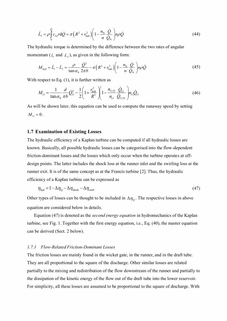
1.7 Examination of Existing Losses

The hydraulic efficiency of a Kaplan turbine can be computed if all hydraulic losses are

known. Basically, all possible hydraulic losses can be categorised into the flow-dependent

friction-dominant losses and the losses which only occur when the turbine operates at off-

design points. The latter includes the shock loss at the runner inlet and the swirling loss at the

runner exit. It is of the same concept as at the Francis turbine [2]. Thus, the hydraulic

efficiency of a Kaplan turbine can be expressed as

hyd Q shock swirl1 = − − − (47)

Other types of losses can be thought to be included in Q . The respective losses in above

equation are considered below in details.

Equation (47) is denoted as the second energy equation in hydromechanics of the Kaplan

turbine, see Fig. 1. Together with the first energy equation, i.e., Eq. (40), the master equation

can be derived (Sect. 2 below).

1.7.1 Flow-Related Friction-Dominant Losses

The friction losses are mainly found in the wicket gate, in the runner, and in the draft tube.

They are all proportional to the square of the discharge. Other similar losses are related

partially to the mixing and redistribution of the flow downstream of the runner and partially to

the dissipation of the kinetic energy of the flow out of the draft tube into the lower reservoir.

For simplicity, all these losses are assumed to be proportional to the square of discharge. With

the cross-sectional area of the flow at the runner (A) as reference, the sum of frictional and

flow-related internal losses is, then, represented as

2

Q Q1

2Q

gH A

=

(48)

Here, Q is the head drop coefficient.

With respect to the definition of unit discharge according to Eq. (1) and because of

( )2 2hubA R r= − , the above equation is also written as

( )

Q 2Q 112 22 2

hub

16

1Q

r R

=

− (49)

The pressure drop coefficient Q can be determined from the nominal operation point, at

which the hydraulic efficiency, for instance, is known as hyd,N 0.9 = . Then from Eq. (41), the

nominal discharge NQ or 11,NQ is computed. Finally, one obtains the pressure drop coefficient

Q from Eq. (48) or Eq. (49) with Q,N hyd,N1 0.1 = − = .

1.7.2 Shock Loss at the Runner Inlet

The shock loss is related to the flow at the runner inlet and occurs at off-design points of the

Kaplan turbine. It arises from the abrupt change in the direction of the flow and so from the

flow separation along the leading edge of each runner blade and subsequent redistribution of

the flow within the blade channels. The mechanism of leading to hydraulic loss is the same, as

the Borda–Carnot shock loss relies on.

According to Fig. 4, in which the velocity triangle is shown for a partial load, the shock

loss in form of the head drop is given by

( )

gwh 2

21

shshock

= (50)

The coefficient sh accounts for the part of the shock loss at the theoretical maximum.

Then, the shock loss is expressed in term of efficiency loss as Hhshockshock = . Based

on the geometrical relation presented in Fig. 4 and by applying the relative velocity 1w , the

shock loss is further expressed as

( )22 2 2

1 1b 1 mshock sh sh2

1b 1b 1

sin 1 1sin 2 tan tan 2

w cgH gH

− = = −

(51)

Here, 1b represents the design angle of runner blades on their leading edge. Only when the

flow angle 1 equals the blade angle 1b , the shock loss vanishes.

In using of the definition of unit discharge 11Q , the meridian velocity mc is further

expressible as

( )

2 2m 11

22 2 2hub

162 1

c QgH r R

=−

(52)

Substituting this equation into Eq. (51) yields

( )

2 211

shock sh 22 2 21b 1 hub

161 1tan tan 1

Q

r R

= −

− (53)

For 1tan and 1btan in above equation, one obtains from Eq. (14) with respect to 1b for

nominal operation

2

11,N2 hub113 2

1b 1 11,N 11 0,N 0

1 1 2 1 1 1 1tan tan 2 tan tan

n rnrRd Q Q br R

− = − − − −

(54)

Thus, the shock loss is further written as

22

11,N 2sh 11shock 112

11,N 11 0,N 0

2 1 12 tan tan

n nr d Qd Q Q br

= − − −

(55)

The shock loss is directly related to the control parameter 0 , but is still a function of the

radial coordinate. Its mean value is obtained by the integration

hub

shock shock m1 2 d

R

r

rc rQ

= (56)

This leads to

( )

( )

22

11,Nshock hub 112 2

sh 11 11,N 11

11,N 11

11,N 11 0,N 0

22

hub2 2 2

0,N 0 hub

1 12

2 1 1 tan tan

ln2 1 1 tan tan 1

nr nQ R Q Q

n ndb Q Q

R rdr Rb

= + −

− − −

+ − −

(57)

Except for 11Q and 11n , all other parameters in this equation are referred to either the

nominal operation or geometrical specifications. They can, thus, be considered as given.

Equation (57) will be used in connection with the swirling loss at the runner exit to

compute the main loss in the Kaplan turbine for both the partial load and the overload.

1.7.3 Swirling Loss at the Runner Exit

In this section, only the runner with fixed blades is considered.

At partial load or overload, the exit flow out of the runner possesses a circumferential

velocity component, see Eq. (21). The kinetic energy contained in this swirling flow will be

dissipated in the downstream draft tube and thus should be basically considered as being lost.

Because of the non-uniform distribution of the circumferential velocity component c2u, as

given in Eq. (21), the averaged mean of the kinetic energy is obtained through integration.

This is given as

( )

hub

222 2N2u m

N

21 11 2 d2 2

R

r

n n Qc r rc rn Q Q

= −

(58)

By assuming the uniform axial velocity component cm, one obtains

( )

22 22 hub N2u 2

N

1 1 12 4

dn r n QcR n Q

= + −

(59)

The corresponding efficiency loss is further computed. Using the unit parameters defined in

Eq. (1) follows

2

22 2hub 11 11

swirl 2u 11,N211,N 11,N

1 1 12 2

r n Qc ngH R n Q

= = + −

(60)

It is worth noting that between Eqs. (37) and (59) the following relation can be found:

212u N2

N2u

1 12

c n Qn Quc

= −

, (61)

which is similar to that at the Francis turbine [2].

2 Master Equation of the Kaplan Turbine The first and second energy equations have been derived in Eqs. (40) and (47), respectively.

To Eq. (47), corresponding terms have also been worked out in detail. In this section, as

indicated in Fig. 1, the master equation of the Kaplan turbine will be presented.

2.1 Discharge Combining Eqs. (40) and (47) to collect all partial losses, one obtains, after proper

rearrangement

2A 11 B 11 C 0k Q k Q k+ + = (62)

with

( )

( )

22Q11,Nsh hub

A 22 2 2 2 211,N hub

2211,N hubsh

sh 2 20,N 0 11,N 0,N 0 hub

1 1612 1

ln2 1 1 2 1 1tan tan 2 tan tan 1

nrkR Q r R

n R rd db Q b r R

+= + +

−

− − + − −

2

11,Nsh sh hubB 11 sh 112

0,N 0 11,N

12 1tan tan

nrdk n nb R Q

−= + − +

( )2

2hubC sh 112

1 1 1 12

rk nR

= − − + −

This equation is called the master equation of the Kaplan turbine. It is a simple quadratic

polynomial for the unit discharge 11Q , comparable to the master equation of the Francis

turbine [2]. All three coefficients are simply a function of the rotational speed 11n and the

guide-vane angle 0 . Because other parameters are either geometrical parameters or

parameters related to the nominal operating point, the master equation basically represents a

function of ( )11 0 11f ,Q n= , with 0 as the regulation or control parameter.

The expressions of all three coefficients appear to be somewhat complex. This is because

they all account for the outcomes of viscous friction effect, shock and swirling losses, which

are of different fluid mechanics. For approximation, sh 1 is applicable. Then, both the

coefficients kB and kC can be considerably simplified. The assumption of Q 0 = , however, is

basically not admissible, because at the Kaplan turbine the volume flow rate is commonly

high and so is the resultant loss. The author would like to emphasize that no any other

mathematical approximations should be made, because the master equation exactly represents

a closed solution of the Kaplan turbine and thus always provides reasonable computational

results.

The expression 11,N 11,Nn Q in both coefficients Ak and Bk can be replaced by the nominal

discharge coefficient N according to Eq. (6).

The nominal discharge is obtained under the nominal guide-vane opening 0,N directly

from Eq. (41) with hyd,N 0.9 = , for instance. When the master equation is applied, the

computation finally leads to Eq. (41) as well.

At 011 =n , it is about a free-flow process through the Kaplan turbine. The unit discharge

is obtained in this case as

11,n=0A

1Qk

= . (63)

Because of the composition of the coefficient Ak , the discharge at 0=n is primarily

determined by the shock loss at the runner inlet and the swirling flow at the runner exit. The

discharge will be considerably reduced, see also the computational example below in Sect.

2.5.

At the nominal setting of guide vanes ( 0,N ) and by neglecting the friction-dominant

losses ( 0Q ) as well as with sh 1 , the coefficient Ak is simplified to

2211,Nhub

A,N 2 211,N

1nrk

R Q

+

(64)

With respect to both 11,NQ according to Eq. (1) and 2N 11,N1 n = according to Eq. (4), the

ratio of the free flow through the Kaplan turbine to the nominal discharge is obtained from

Eq. (63)

0.5

n=0,N N2 2

N hub1Q

Q r R

+

(65)

For N 0.3 = and hub 0.43r R = , for instance, one obtains n=0,N N 0.5Q Q , corresponding to a

reduction in discharge by a factor 2. This is the reason, why in Eq. (64) the approximation of

0Q has been applied.

On the other hand, the unit discharge given in Eq. (63) can also be directly obtained from

Eq. (57) for shock loss, from Eq. (60) for swirling loss and from Eq. (49) for flow-dependent

friction loss by setting 011 =n and subsequently using 1Qswirl,0shock,0 =++ . Thus, the

free discharge at 011 =n is completely governed by shock, swirling, and friction losses. The

last factor is, as just shown above, mostly negligible.

2.2 Hydraulic Efficiency The hydraulic efficiency of a Kaplan turbine is given, once the discharge has been computed

from Eq. (62) and subsequently inserted into Eq. (40). In the practice, it has often been shown

in form of a hill chart. The related computations will be presented below in Sect. 2.5 in

association with a computation example.

2.3 Hydraulic Torque and Power Accounting for the hydraulic efficiency, the hydraulic power of a Kaplan turbine is computed

as

QgHP hydhyd = (66)

The computation of the hydraulic efficiency is referred to Eq. (40) or, equivalently, to Eq.

(47).

On the other hand, the hydraulic power is represented as the product of the hydraulic

torque exerted on the shaft (moment hydM ) and the angular speed (2 n ) of the shaft, as given

by hydhyd 2 nMP = . By equalising this equation with Eq. (66) and further by applying Eq. (1),

one obtains

hyd 1111

112QMn

= (67)

In this equation, the unit discharge ( )11 11 0f ,Q n = has already been computed by the master

equation, viz. Eq. (62).

Furthermore, from Eq. (2) the power coefficient 11 is also obtainable.

Equation (67) in its given form could not be directly applied to the case 0=n . From Eq.

(46), however, one obtains immediately

2

11,N 2hub11,n=0 11,n=02

0 11,N

1 1 1tan 2

nrdM Qb R Q

= + +

(68)

For 11,n=0Q refer to Eq. (63).

For nominal setting of guide vanes ( 0,N ) and in applying Eq. (67), one obtains the ratio of

the torque to the nominal torque under the nominal operating condition:

2 2

11,n=0,N 11,n=0,N 11,N 11,Nhub2

11,N hyd,N 11,N 0,N 11,N

2 1 1 1tan 2

M Q n nrdM Q b R Q

= + +

(69)

The term 0,Ntan is substituted by Eq. (41), yields

22

11,n=0,N 11,n=0,N 2hub11,N2 2 2

11,N 11,N hyd,N 11,N

1 11M Qr n

M n R Q

= + +

(70)

When using respective physical quantities ( hyd,NM and NQ ) and the approximation of Eq.

(65), one obtains with further consideration of 211,N N1n =

hyd,n=0,N N2 2

hyd,N hub hyd,N

11

MM r R

+

+ (71)

It is a function of the geometric design of the Kaplan turbine.

2.4 Reconstruction of the Master Equation The master equation in the given form at Eq. (62) is suitable to compute characteristics of the

Kaplan turbine in the basic form of discharge ( )11 11 0f ,Q n = and subsequently also of other

operation parameters like efficiency hyd and power coefficient 11 . Computation examples

will be shown in Sect. 2.5. Sometimes, as for special applications, the master equation needs

to be reformed. This has been demonstrated to be much helpful at the Francis turbine, when

hydraulic transients in a hydraulic system with Francis turbines should be computed [13].

For extended applications, therefore, the master equation given at Eq. (62) is reformed to

( )2 22 11 1 11 11 0 11 1 0m Q m n Q m n+ + − = (72)

The corresponding coefficients 2m , 1m and 0m can be obtained from the coefficients Ak , Bk

and Ck as follows:

2 Am k=

1 B 11m k n=

( )2

C hub0 sh2 2

11

1 1 1 12

k rmn R

+

= = − − +

All these three coefficients do not contain the unit speed 11n . Especially for sh 1 there is

0 0m = . Correspondingly, the coefficient 1m is simplified to

2

11,NhubB1 2

11 0,N 11,N

2 1 1tan

nrk dmn b R Q

= = − +

(73)

It is even independent of the control parameter 0 of guide vanes at the wicket gate.

The reconstructed master equation has applications in computations of hydraulic

transients which are caused, for instance, by starting, stopping, or regulating the turbine load

in a hydraulic system with Kaplan turbines. Another application is the computation of the

runaway speed of the Kaplan turbine, as will be shown below in Sect. 3.

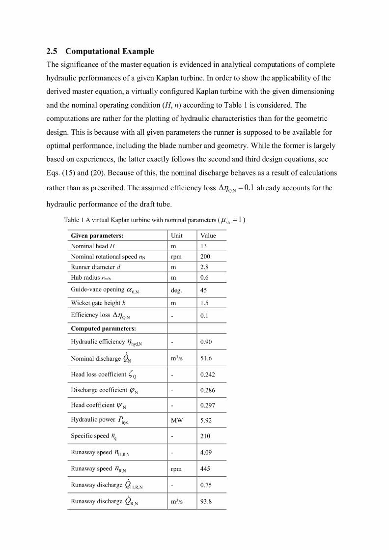
2.5 Computational Example The significance of the master equation is evidenced in analytical computations of complete

hydraulic performances of a given Kaplan turbine. In order to show the applicability of the

derived master equation, a virtually configured Kaplan turbine with the given dimensioning

and the nominal operating condition (H, n) according to Table 1 is considered. The

computations are rather for the plotting of hydraulic characteristics than for the geometric

design. This is because with all given parameters the runner is supposed to be available for

optimal performance, including the blade number and geometry. While the former is largely

based on experiences, the latter exactly follows the second and third design equations, see

Eqs. (15) and (20). Because of this, the nominal discharge behaves as a result of calculations

rather than as prescribed. The assumed efficiency loss Q,N 0.1 = already accounts for the

hydraulic performance of the draft tube.

Table 1 A virtual Kaplan turbine with nominal parameters ( sh 1 = )

Given parameters: Unit Value Nominal head H m 13 Nominal rotational speed nN rpm 200 Runner diameter d m 2.8 Hub radius rhub m 0.6

Guide-vane opening 0,N deg. 45

Wicket gate height b m 1.5

Efficiency loss Q,N - 0.1

Computed parameters:

Hydraulic efficiency hyd,N - 0.90

Nominal discharge NQ m3/s 51.6

Head loss coefficient Q - 0.242

Discharge coefficient N - 0.286

Head coefficient N - 0.297

Hydraulic power hydP MW 5.92

Specific speed qn - 210

Runaway speed 11,R,Nn - 4.09

Runaway speed R,Nn rpm 445

Runaway discharge 11,R,NQ - 0.75

Runaway discharge R,NQ m3/s 93.8

While the nominal discharge NQ is computed from Eq. (41), the pressure drop coefficient Q

is determined from Eq. (48).

Fig. 5 Characteristics of the Kaplan turbine as functions of the unit speed and the guide-vane opening (GO), computed from the master eqution

Figure 5 shows computational results regarding unit discharge, unit momentum, hydraulic

efficiency, and power coefficient. The efficiency hill chart has also been shown. Following

remarkable points can be drawn:

• The sensitivity of load regulation is smaller at large guide-vane angles ( 0 ). This

implies that for setting the nominal guide-vane opening, one should always carry out

corresponding computations regarding the regulation sensitivity. After 0,N has been

chosen, the first design equation (42) can be applied to size the Kaplan turbine by

computing the parameter b. For better applications, both parameters should be optimized

by combining them.

• From the diagram ( )11 11 0f ,Q n = , one reads out that for the nominal opening of guide

vanes (100% GO) the ratio of the free flow through the turbine (n=0) to the nominal

discharge is about 0.5. This accurately agrees with the value which is calculated from

Eq. (65).

• From the diagram ( )11 11 0f ,M n = , one reads out that again for the nominal opening of

guide vanes (100% GO) the hydraulic torque at n=0 is about 1.33 times of the torque

under the designed operating point. This agrees well with the computation of Eq. (71)

leading to a torque ratio of 1.36.

• At the design point, the hydraulic efficiency measures 90%. It agrees with the given

value in Table 1. One confirms that a small reduction of the unit number from the

nominal value even leads to an increase in the efficiency. This is simply because of the

dominant reduction of the friction-dependent loss Q , while the increase of other two

losses ( shock and swirl ) are negligible. Therefore, the best efficiency point (BEP) of

a Kaplan turbine, commonly and accurately, always slightly differs from the design

point.

• At n=0, the gradient of the efficiency curve can be computed from Eq. (40) as

2

hyd 11,Nhub11,n=02

11 0 11,Nn=0

d 2 1 1d tan

nrd Qn b R Q

= + +

(74)

If compared with Eq. (68), one obtains

hyd 11,n=0

11 11,n=0n=0

d2

dM

n Q

= (75)

It appears to be a logical result as from Eq. (67).

Further, the nominal setting of guide vanes is considered. In view of Eq. (41), the above

equation becomes

2

hyd hyd,N 11,n=0,Nhub11,N2

11 11,N 11,Nn=0,N

d1

dQr n

n n R Q

= + +

(76)

Then, with respect to Eq. (65) as an approximation and 2N 11,N1 n = , one finally obtains

2

hyd hyd,N N hub22 2

11 n=0,N hub

d1

d 1r

n Rr R

+ +

+ (77)

Basically, if Q 0 = would be true rather than an approximation, then hyd,N 1 = should

be applied.

In the current computational example, a gradient of ( )hyd 11 n=0,Nd d 1.333n = is directly

obtained from above equation, as shown in the diagram. It approximately also applies to

other guide-vane settings. Especially, the above equation can be applied, for instance, to

extrapolate measurements to n=0 and to create regression curves.

• For the curve of runaway (M=0) in diagram ( )11 11 0f ,Q n = , see Sect. 3 below.

The characteristics of the Kaplan turbine describe the turbine performances under the

operating conditions out of the design point. The associated remarkable occurrences in the

flow are the shock and swirling losses, as described in Sect. 1.7. In the computational example

presented here, these two types of losses have also been computed, as shown in Fig. 6 for a

guide-vane setting of 0 30 = . It is obvious that both the shock and swirling losses dominate

at both partial and overloads.

Fig. 6 Main losses in the considered Kaplan turbine at a partial load which is given by the guide-vane opening of 0=30°

3 Runaway Speed of the Kaplan Turbine A special case at the Kaplan turbine is the case of emergency load rejection for some reasons.

The available head and the water flow then force the turbine unit to speed up towards a

maximum which is called the runaway speed.

The maximum runaway speed behaves as a critical value for the mechanical safety of both

the turbine runner and the rotor of the generator. Because under the runaway speed no energy

exchange between the flow and the runner occurs, both the hydraulic efficiency and the torque

vanish ( 0Rhyd, = and 0R,11 =M ). The runaway speed is thus a clearly defined parameter. In

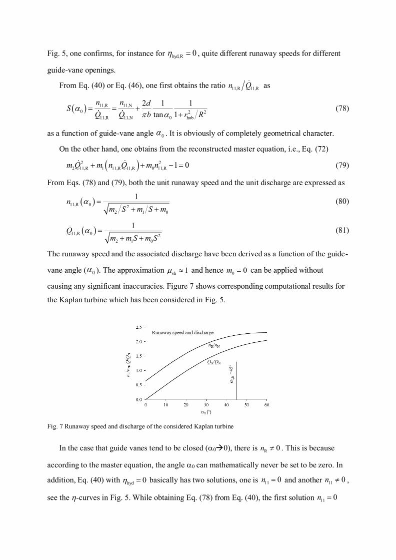
Fig. 5, one confirms, for instance for 0Rhyd, = , quite different runaway speeds for different

guide-vane openings.

From Eq. (40) or Eq. (46), one first obtains the ratio 11,R 11,Rn Q as

( ) 11,R 11,N0 2 2

11,R 11,N 0 hub

2 1 1tan 1

n n dSQ Q b r R

= = ++

(78)

as a function of guide-vane angle 0 . It is obviously of completely geometrical character.

On the other hand, one obtains from the reconstructed master equation, i.e., Eq. (72)

( )2 22 11,R 1 11,R 11,R 0 11,R 1 0m Q m n Q m n+ + − = (79)

From Eqs. (78) and (79), both the unit runaway speed and the unit discharge are expressed as

( )11,R 0 2

2 1 0

1nm S m S m

=+ +

(80)

( )11,R 0 22 1 0

1Qm m S m S

=+ +

(81)

The runaway speed and the associated discharge have been derived as a function of the guide-

vane angle ( 0 ). The approximation sh 1 and hence 0 0m = can be applied without

causing any significant inaccuracies. Figure 7 shows corresponding computational results for

the Kaplan turbine which has been considered in Fig. 5.

Fig. 7 Runaway speed and discharge of the considered Kaplan turbine

In the case that guide vanes tend to be closed (0→0), there is R 0n . This is because

according to the master equation, the angle 0 can mathematically never be set to be zero. In

addition, Eq. (40) with hyd 0 = basically has two solutions, one is 11 0n = and another 11 0n ,

see the -curves in Fig. 5. While obtaining Eq. (78) from Eq. (40), the first solution 11 0n =

has been erased. From Eq. (78) and (79), one in effect obtains another solution 11,R 0n , i.e.,

Eq. (80).

It should be mentioned that up to now the runaway speed of the Kaplan turbine has often

been given in the form of NR nn . In [14], for instance, the runaway speeds of the Kaplan

turbine have been indicated to be R N 2.0 2.6n n = − (Kaplan single regulated). First, this

indication is much coarse, since the deviation from the median (2.3) is exceedingly high (

13% ). Second, the dependence of the runaway speed on the guide-vane settings has not been

included.

It should be further mentioned that Eqs. (80) and (81) also apply to the Francis turbine.

One only needs to use the respective parameter S. In [2], because the reconstructed master

equation of using coefficients 0m , 1m und 2m had not been given explicitly, the computation

of the runaway speed has been expressed in another form. For the computation of the

parameter S, the ratio 11,R 11,Rn Q has been given in [2]. It is very similar to Eq. (78).

The special case of nominal opening of guide vanes is now considered.

From Eq. (78) one obtains

( ) 11,N0,N 2 2

11,N 0,N hub

2 1 1tan 1

n dSQ b r R

= ++

(82)

The term 0,Ntan will be replaced by that from Eq. (41). This leads to

( )2

hyd,N 11,Nhub0,N 2 2 2 2

11,N 11,N hub

111

nrSn R Q r R

= + + +

(83)

It should be remined that the efficiency hyd,N under the nominal operating condition behaves

as a given parameter like N and N . In the considered example in Sect. 2.5, it is hyd,N 0.9 =

according to Table 1. Then, with respect to Eq. (6) and 2N 11,N1 n = , one further obtains

( ) hyd,N N0,N 2 2

hub N

4 111

Sr R

= +

+ (84)

It is now completely related to the turbine runner. Hence, all following computations can also

be applied to other types of Kaplan turbines like the bulb turbine, see Sect. 4 below.

While using m0=0, the coefficient m1 is likely computed from Eq. (73) with respect to Eq.

(41):

2 2

hyd,N 11,Nhub hub1 hyd,N N2 2 2

11,N 11,N N

4 11 1nr rm

n R Q R

= − + = − +

(85)

For the computation of m2 with 2 Am k= , it follows from Eq. (62), again with respect to Eq.

(6)

( ) ( )

22 2Q Q11,Nhub hub

2 2 22 2 2 2 2 2 22 2 2 211,N Nhub hub

16 16 1 161 11 1

nr rmR Q Rr R r R

= + + = + + − −

(86)

The question arises whether the approximation Q 0 = can be applied. The use of the

approximation certainly leads to the overestimation of the runaway speed. Because the

discharge under the condition of runaway speed is significantly large, see 11Q -curve in Fig. 5,

the viscous friction effect ( Q 0 ) could be incredibly large. This can be verified through

comparison between computations with and without the approximation, respectively. The

difference is found only in the coefficient m2, i.e., the last term in Eq. (86). For the considered

computation example, the overestimations of both the runaway speed and the discharge are of

about 10%. Obviously, this is unfortunately a bit too large.

Only for the purpose of completeness of theoretical analyses, the outcome of Q 0 = and

hence of hyd,N 1 = is given here. First, one obtains

2 2

N hub2 12 2 2 2

hub N

11

rm mS S r R R

+ = +

+ + (87)

2

N2 1 2 2

N hub

4 11

m m Sr R

+ =

+ (88)

Then, it follows from Eqs. (80) and (81), respectively, with m0=0

( )

2 2hub

11,R 0,N 2 2N hub

1 11

r Rn

r R

+= +

+ (89)

( )2

hub N11,R 0,N 2

N

14

rQR

= + (90)

When to these two equations the relation 2N 11,N1 n = and Eq. (6) are applied, then the

runaway speed and discharge, related to the nominal values, are computed as

2 2R,N hub N

2 2N N hub

11

n r Rn r R

+= +

+ (91)

2

R,N hub2

N N

1 1Q rQ R

= +

(92)

In the considered example (Fig. 5), these two equations have led to R,N 500n = rpm and

R,N 103Q = m3/s, respectively. If compared with true values in Table 1, the respective

overestimations are about 10% and 12%. As said above, these two values appear to be a bit

too large, so that Eqs. (89) to (92), based on the approximation Q 0 = , should not be simply

used for the Kaplan turbine.

An interesting relation is found, if Eq. (91) is compared with Eq. (77). For hyd,N 1 =

which is based on Q 0 = , one obtains

hyd R,NN

11 Nn=0,N

dd

nn n

= (93)

The physical background of this relation, however, is not yet clear.

Another interesting relation is further found, if Eq. (92) is compared with Eq. (65):

R,N N

N n=0,N

Q QQ Q

= or N R,N n=0,NQ Q Q= (94)

The nominal discharge NQ is the geometric mean of the runaway discharge R,NQ and the free-

flow discharge n=0,NQ .

Other special relations can also be obtained, for instance, from Eq. (71) for hyd,N 1 = and

Eq. (92).

4 Other Types of Kaplan Turbines In all computations in Sect. 1, which lead to the establishment of the master equation, the

employed control parameter is the guide-vane opening 0 , see Fig. 2. For other forms of the

Kaplan turbine, like the bulb turbine and those with guide vanes being placed close to the

runner (Fig. 8), the control parameter 0 can no longer be applied. In order to make further

use of all computations in the above sections, a new and equivalent control parameter must be

redefined.

For this purpose, the mean radius mr is introduced as the reference radius, which divides

the flow area into two equal sub-areas ( ) ( )2 2 2 2m hub mr r R r − = − . It is then computed as

2 2

hubm 2

R rr += (95)

Fig. 8 Kaplan turbine with adjustable guide vanes close to the runner in the same tube

To replace the control parameter 0 , which is found in Fig. 2, one first obtains from Eq. (11)

2

hubm0 2

1u

2 tan 1 rcb RR rc R

= −

(96)

In all computations carried out in Sect. 1 to Sect. 3, the property of the precise potential flow

in the cross-section ahead of the turbine runner has been made use of. At the Kaplan turbine

shown in Fig. 8, however, the exact and comparable potential flow distribution could not be

obtained at operations outside of the design point (this will be demonstrated below). This

determines that interaction between the flow and the turbine runner in case of Fig. 8 differs

from that in case of Fig. 2. The flow basically becomes undescribable. For the sake of

simplicity of computations, the flow after passing through the guide vanes can still be

approximated to be a potential flow. This simply means that the distribution of the

circumferential velocity component is describable by the relation 1u m 1u,mrc r c= , with 1u,mc as

the velocity component found at the mean radius mr . Then, Eq. (96) is further written as

2 2

hub hubm0 1m2 2

1u,m m m

2 tan 1 tan 1r rcb R RR c r R r R

= − = −

(97)

2rm

c1u,m

section 1

run

ner

section 1

section 2

d=2R n

draf

t tu

be

GV

2rhub

rm

In principle, the flow angle 1m in cross-section 1 is determined by the guide-vane angle

GVm at the radius mr on the trailing edge of the blade. With GVm 1m = , the above equation

is also written as

2

hub0 GVm 2

m

2 tan tan 1 rb RR r R

= −

(98)

Correspondingly, there follows for the nominal operating point

2

hub0,N GVm,N 2

m

2 tan tan 1 rb RR r R

= −

(99)

In all computations from Sect. 1 to Sect. 3, expressions ( ) 02 tanb R and ( ) 0,N2 tanb R can

be replaced by the respective last terms in the above two equations. In this way, a new control

parameter for load regulation is found to be GVm at the radius mr . Its nominal setting is

GVm,N . All relevant hydraulic characteristics, like that in Figs. 4, 5 and 6, can be computed

and redrawn in terms of guide-vane settings GVm .

In analogy to Eq. (42), the first design equation of the current Kaplan turbine can be

derived based on the use of design parameter N Nn Q gH . This is obtained from Eqs. (42) and

(99):

N NmGVm,N 2 2

hyd,N hub

2 1tan1

n QrRR r R gH

=−

(100)

After having selected the hub-diameter ratio hubr R and hence mr R , the size of the Kaplan

turbine is determined in terms of GVm,NtanR .

The concept of designing the guide vanes is again focused to creation of potential flows at

the exit of guide-vane channels. The relevant circumferential velocity component and its

radial distribution are obtained from Eq. (96) and Eq. (99), both for the nominal operation:

m,NGVm,N

1u,N m

tanc rc r

= (101)

It represents the flow angle in form of 1,Ntan as a function of the radial coordinate. For

blade-congruent flows there must be 1,N GV,N = . Thus, one obtains

GV,N GVm,Nm

tan tanrr

= (102)

This is the design equation of guide vanes. The twist angle of blades along the blade trailing

edge, in form of GV,Ntan , linearly changes with the radial coordinate.

The fact to be mentioned is that the related design rule only ensures the swirl flow with

1u,N 1c r for the circumferential velocity component under the nominal operating condition.

At other operating points in case of load regulation, the desired swirl flow distribution cannot

be accurately achieved. This is different from the regulation behaviour of the Kaplan turbine

that has been shown in Fig. 2 and considered in previous sections. This can be demonstrated

by considering Eq. (102) as follows:

Supposing that the opening of guide vanes is changed by GV for the purpose of turbine

load regulation. Then, both the distribution angle ( )GV,N r and the fixed angle GVm,N in Eq.

(102) change to GV,N GV + and GVm,N GV + , respectively. Because with these two new

values Eq. (102) cannot hold and thus becomes invalid, the blade-congruent flow out of the

guide vanes is no longer equal to the distribution of a potential flow. This flow dynamics is

related to the occurrence of energy losses in the flow while passing through the guide vanes.

On the other hand, however, if these losses are negligible, then the exit flow out of guide

vanes will tend to be redistributed by itself to meet the potential flow profile ( 1u,N 1c r ). For

simplicity of computations, especially for direct applications of all computations performed in

Sect. 1 to Sect. 3, potential flow profiles at the exit of guide vanes can still be supposed.

Figure 9 shows the computed velocity distributions, respectively, for the nominal and a

partial opening of guide vanes (63% GO). The Kaplan turbine considered is the same as used

in Fig. 5 in accordance with Table 1, however, with the guide vanes being placed close to the

runner (Fig. 8). Obviously, the exit flow out of the guide vanes with 63% GO has

satisfactorily agreed with the profile of potential flows.

Fig. 9 Velocity profile at the exit of guide vanes of a Kaplan turbine according to Fig.8.

In summary, all computations carried out in Sect. 1 to Sect. 3 can be applied to the current

case with adjustable guide vanes according to Fig. 8. One only needs to use the substitutions

of Eqs. (98) and (99). The new control parameter is now the guide-vane angle GVm .

For Kaplan turbines with adjustable runner blades, both the master equation and the

runaway speed must be completely recalculated.

5 Summary The main objective of the current paper is focused on the creation of the master equation of

the Kaplan turbine. For better understanding and applications, computations similar to that for

the Francis turbine [2] has been completed.

First, the nominal operation of the turbine has been extended to involve the variation of

both the hydraulic head and the runner rotational speed. With the introduction of a new design

parameter in place of the specific speed, three design equations have been presented for

dimensioning the Kaplan turbine and configuring blade profiles.

Furthermore, based on averaging of the Euler equation and accurate computations of both

the shock and the swirling losses, two energy equations are formed, from which the master

equation of the Kaplan turbine has been created. The master equation uniquely combines the

geometric design of the turbine runner with the dynamic operations of the turbine unit, so that,

for the first time, the complete characteristics of the Kaplan turbine can be analytically

computed. The master equation in a reconstructed form, additionally, permits the accurate

determination of the runaway speed, explicitly, as a function of the guide-vane settings. Just

because of this functional dependence, the computational accuracy is at least one order higher

than that found in the literature and handbooks.

All computations leading to the master equation and successive equations can also be

applied to the bulb turbine and other types of Kaplan turbines with guide vanes ahead of the

turbine runner in the same tube. The corresponding substituting control parameter has been

given.

Many special cases like the free flow through the turbine at n=0 have been considered. All

simplified relations can be applied to validate designs and CFD simulations. For the latter,

then, validations through expenditure experimental measurements would become

unnecessary.

The author kindly and appreciatively asks the interested readers or researchers to make

validations of the method presented in this paper with their experimental data.

References

[1] Zhang Zh. Pelton Turbines [M]. Cham, Switzerland, Springer-Verlag, 2016. [2] Zhang Zh. Master equation and runaway speed of the Francis turbine [J]. J Hydrodyn

30, 203–217 (2018). [3] Gieseck, J., Mosonyi E. Wasserkraftanlagen [M]. 6. Auflage, Springer-Verlag, 2014. [4] Bohl W. Strömungsmaschinen 2 [M]. 8. Auflage, Vogel Fachbuch, 2012. [5] Quantz L., Meerwarth K. Wasserkraftmaschinen [M]. 11. Auflage, Springer-Verlag,

1963. [6] Jehle, C. Bau von Wasserkraftanlagen [M]. 6. Auflage, Berlin, Offenbach, VDE Verlag,

2016. [7] Rai, A., Kumar, A. Analyzing hydro abrasive erosion in Kaplan turbine: A case study

from India (J). J Hydrodyn, 28, 863-872 (2016). [8] Tran, C.T., Long, Xp., Ji, B. et al. Prediction of the precessing vortex core in the

Francis-99 draft tube under off-design conditions by using Liutex/Rortex method [J]. J Hydrodyn 32, 623–628 (2020).

[9] Yang, J., Zhou, Lj. & Wang, Zw. Numerical investigation of the cavitation dynamic parameters in a Francis turbine draft tube with columnar vortex rope [J]. J Hydrodyn 31, 931–939 (2019).

[10] Mulu BG., Cervantes MJ., Devals C. et al. Simulation-based investigation of unsteady flow in near-hub region of a Kaplan Turbine with experimental comparison [J]. Engineering Applications of Computational Fluid Mechanics, March 2015.

[11] Muntean S., Balint D., Susan-Resiga R. et al. 3D Flow Analysis in the Spiral Case and Distributor of a Kaplan Turbine [C]. 22nd IAHR Symposium on Hydraulic Machinery and Systems, Stockholm, Sweden, 2004.

[12] Muntean S., Balint D., Susan-Resiga R. et al. Analytical representation of the swirling flow upstream the Kaplan turbine runner for variable guide vane opening [C]. 23rd IAHR Symposium on Hydraulic Machinery and Systems, Yokohama, Japan, 2006.

[13] Zhang Zh. Hydraulic Transients and Computations [M]. Switzerland, Springer-Verlag, 2020.

[14] ESHA. Guide on how to develop a small hydropower plant. European Small Hydropower Association (ESHA), 2004.