Embed Size (px)
Citation preview
Master of Science Thesis
at Mälardalen University, Sweden
GRETA
A tool concept for validation/veri�cation
of signal based systems (e.g. PLEX)
Andreas Arnström [email protected]
Camilla Grosz [email protected]
Andreas Guillemot [email protected]
May 18, 2000

Abstract
The main part of the software in the Ericsson AXE telecommunication system is
based on an event based real-time language called PLEX. In this Master thesis
the main subjects are to add the possibility of abstraction and analysis of systems
written in PLEX. GRETA (GRaphical Extractor and Time Analyzer) enables the
programmer to view and explore the system graphically and browse the system
on di�erent abstraction levels. The graph shows time data for signals. It enables
programmers to �nd unoptimized parts, dead ends, loops and to understand the
behavior of the system on the signal level.
To achieve this we have analyzed graphical representation for systems written
in PLEX and execution time calculation for PLEX code. A prototype for execution
time calculation and graphical abstraction of systems written in PLEX has been
implemented. In the analysis part, we compare PLEX with other programming
languages and system paradigms, both traditional programming languages and new
concepts, ideas and notations. We also investigate advantages and disadvantages
with PLEX and systems based on PLEX.
In the PLEX environment everything is centered around asynchronous signal
communication. Code-items, large function blocks and sub-systems are communi-
cating with each other using signals. This code structure can be quite complex
and hard to survey for programmers (telecommunication systems are very large
and complex in themselves). GRETA is structured in three parts, a Facts Finder,
a Structure Finder and a Graph Finder. The Facts Finder extracts necessary in-
formation from PLEX code and the compiler. It is not implemented, because it
is beyond the scope of this thesis, though it is discussed in theory. The Structure
Finder (implemented in Prolog) uses output (a well speci�ed data �le) from the
Facts Finder. The program is able to capture the signaling connections between
the function blocks and the code-items in the system and then write them struc-
tured to a �le with execution time information for signals and code-items. The
Graph Finder (implemented in Java) can read the structures created by the Struc-
ture Finder and display all connections as graphs in a window. More advanced
execution time calculations are not implemented, but explored in theory.
Acknowledgments
This Master thesis was written at Ericsson Utvecklings AB during the
period between June 1999 and January 2000. The work has been performed
by Andreas Arnström, Camilla Grosz and Andreas Guillemot. It forms a
required thesis for the degree of Master of Science in Computer Science at
Mälardalen University in Västerås, Sweden.
Foremost, the authors would like to thank the supervisors, Peter Funk
at Mälardalen University, Janet Wennersten and Daniel Kroné at Ericsson
UAB.
There are also some people at our department at Ericsson UAB that we
want to thank. Anders Skelander for his support on many of the practical
problems. Lars-Erik Wiman for all info about SDL.
We would also like to thank some people at Mälardalen University. Jan
Gustafsson (execution time calculation), Jukka Mäki-Turja (real-time sys-
tems), Kjell Post (Prolog syntax), Magnus Eriksson (AI-agents), Martin
Skogevall (Java syntax), Mikael Andersson (comments and ideas according
to the report).
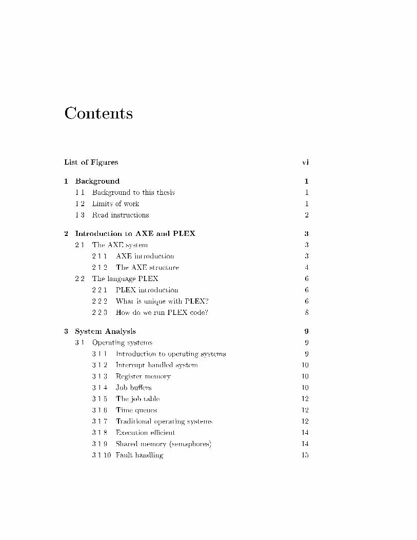
Contents
List of Figures vi
1 Background 1
1.1 Background to this thesis . . . . . . . . . . . . . . . . . . . . 1
1.2 Limits of work . . . . . . . . . . . . . . . . . . . . . . . . . . 1
1.3 Read instructions . . . . . . . . . . . . . . . . . . . . . . . . . 2
2 Introduction to AXE and PLEX 3
2.1 The AXE system . . . . . . . . . . . . . . . . . . . . . . . . . 3
2.1.1 AXE introduction . . . . . . . . . . . . . . . . . . . . 3
2.1.2 The AXE structure . . . . . . . . . . . . . . . . . . . . 4
2.2 The language PLEX . . . . . . . . . . . . . . . . . . . . . . . 6
2.2.1 PLEX introduction . . . . . . . . . . . . . . . . . . . . 6
2.2.2 What is unique with PLEX? . . . . . . . . . . . . . . 6
2.2.3 How do we run PLEX code? . . . . . . . . . . . . . . . 8
3 System Analysis 9
3.1 Operating systems . . . . . . . . . . . . . . . . . . . . . . . . 9
3.1.1 Introduction to operating systems . . . . . . . . . . . 9
3.1.2 Interrupt handled system . . . . . . . . . . . . . . . . 10
3.1.3 Register memory . . . . . . . . . . . . . . . . . . . . . 10
3.1.4 Job bu�ers . . . . . . . . . . . . . . . . . . . . . . . . 10
3.1.5 The job table . . . . . . . . . . . . . . . . . . . . . . . 12
3.1.6 Time queues . . . . . . . . . . . . . . . . . . . . . . . 12
3.1.7 Traditional operating systems . . . . . . . . . . . . . . 12
3.1.8 Execution e�cient . . . . . . . . . . . . . . . . . . . . 14
3.1.9 Shared memory (semaphores) . . . . . . . . . . . . . . 14
3.1.10 Fault handling . . . . . . . . . . . . . . . . . . . . . . 15
ii
3.1.11 Updating during execution . . . . . . . . . . . . . . . 15
3.1.12 System load . . . . . . . . . . . . . . . . . . . . . . . . 16
3.1.13 System clock . . . . . . . . . . . . . . . . . . . . . . . 16
3.2 Signal and process based systems . . . . . . . . . . . . . . . . 16
3.2.1 Signal based systems . . . . . . . . . . . . . . . . . . . 16
3.2.2 Process based systems . . . . . . . . . . . . . . . . . . 17
3.2.3 Process overhead . . . . . . . . . . . . . . . . . . . . . 18
3.3 Real-time systems . . . . . . . . . . . . . . . . . . . . . . . . 19
3.3.1 Introduction to real-time systems . . . . . . . . . . . . 19
3.3.2 Hard and soft real-time systems . . . . . . . . . . . . . 19
3.3.3 The real-time model in PLEX . . . . . . . . . . . . . . 19
3.4 Agent based systems . . . . . . . . . . . . . . . . . . . . . . . 20
3.4.1 Introduction to agents . . . . . . . . . . . . . . . . . . 20
3.4.2 Agents in an AXE system . . . . . . . . . . . . . . . . 21
3.4.3 Agents and object oriented design . . . . . . . . . . . 22
4 Language Analysis 23
4.1 PLEX and traditional programming . . . . . . . . . . . . . . 23
4.1.1 Programming language paradigms . . . . . . . . . . . 23
4.1.2 Procedural and imperative languages . . . . . . . . . . 26
4.1.3 Functional languages . . . . . . . . . . . . . . . . . . . 27
4.1.4 Logic languages . . . . . . . . . . . . . . . . . . . . . . 28
4.2 HL-PLEX . . . . . . . . . . . . . . . . . . . . . . . . . . . . . 29
4.2.1 Introduction to HL-PLEX . . . . . . . . . . . . . . . . 29
4.2.2 Advantages with HL-PLEX . . . . . . . . . . . . . . . 30
4.2.3 Disadvantages with HL-PLEX . . . . . . . . . . . . . . 30
5 Execution Time Calculation 32
5.1 Introduction to execution time calculation . . . . . . . . . . . 32
5.1.1 Current research . . . . . . . . . . . . . . . . . . . . . 32
5.1.2 ILP, a method for execution time calculation . . . . . 33
5.1.3 Tools for execution time calculation . . . . . . . . . . 33
5.2 Problems with execution time calculation . . . . . . . . . . . 34
5.2.1 How to calculate the execution time? . . . . . . . . . . 34
5.2.2 Finding the worst case . . . . . . . . . . . . . . . . . . 35
5.2.3 How to handle loops? . . . . . . . . . . . . . . . . . . 35
5.2.4 Finding ways through the program . . . . . . . . . . . 36
iii
5.2.5 How to handle the GOTO-command? . . . . . . . . . 37
5.3 Accuracy constraints . . . . . . . . . . . . . . . . . . . . . . . 37
5.3.1 Which levels of accuracy are there? . . . . . . . . . . . 37
5.3.2 Which level of accuracy do we choose? . . . . . . . . . 38
6 Graphical Representation 39
6.1 Introduction . . . . . . . . . . . . . . . . . . . . . . . . . . . . 39
6.1.1 Represent PLEX graphically . . . . . . . . . . . . . . 39
6.1.2 Any existing graph standards for PLEX? . . . . . . . . 39
6.2 Automata representation . . . . . . . . . . . . . . . . . . . . . 40
6.3 SDL . . . . . . . . . . . . . . . . . . . . . . . . . . . . . . . . 41
6.3.1 Introduction . . . . . . . . . . . . . . . . . . . . . . . . 41
6.3.2 Structure . . . . . . . . . . . . . . . . . . . . . . . . . 42
6.3.3 Data sending . . . . . . . . . . . . . . . . . . . . . . . 44
6.3.4 Timers . . . . . . . . . . . . . . . . . . . . . . . . . . . 44
6.3.5 Behavior . . . . . . . . . . . . . . . . . . . . . . . . . . 44
6.3.6 Data . . . . . . . . . . . . . . . . . . . . . . . . . . . . 44
6.3.7 SDL-10 . . . . . . . . . . . . . . . . . . . . . . . . . . 44
6.3.8 Advantages with SDL . . . . . . . . . . . . . . . . . . 45
6.3.9 Disadvantages with SDL . . . . . . . . . . . . . . . . . 45
6.4 FDL . . . . . . . . . . . . . . . . . . . . . . . . . . . . . . . . 45
6.5 UML . . . . . . . . . . . . . . . . . . . . . . . . . . . . . . . . 46
6.5.1 Introduction . . . . . . . . . . . . . . . . . . . . . . . . 46
6.5.2 Notation . . . . . . . . . . . . . . . . . . . . . . . . . . 47
6.5.3 UML and AXE-10 . . . . . . . . . . . . . . . . . . . . 49
6.5.4 Advantages with UML . . . . . . . . . . . . . . . . . . 50
6.5.5 Disadvantages with UML . . . . . . . . . . . . . . . . 50
6.6 MSC . . . . . . . . . . . . . . . . . . . . . . . . . . . . . . . . 50
6.7 Petri nets . . . . . . . . . . . . . . . . . . . . . . . . . . . . . 51
6.7.1 The Petri net notation . . . . . . . . . . . . . . . . . . 51
6.7.2 `Black & White' and `Coloured' Petri nets . . . . . . . 53
6.7.3 Timed and Stochastic nets . . . . . . . . . . . . . . . . 53
6.7.4 Advantages with Petri nets . . . . . . . . . . . . . . . 54
6.7.5 Disadvantages with Petri nets . . . . . . . . . . . . . . 54
6.7.6 Tools for Petri nets . . . . . . . . . . . . . . . . . . . . 54
6.7.7 Petri nets in PLEX environment . . . . . . . . . . . . 54
iv
7 Prototypes 56
7.1 GRETA . . . . . . . . . . . . . . . . . . . . . . . . . . . . . . 56
7.2 Facts Finder . . . . . . . . . . . . . . . . . . . . . . . . . . . . 58
7.2.1 Storing the facts . . . . . . . . . . . . . . . . . . . . . 58
7.2.2 Execution time calculation . . . . . . . . . . . . . . . . 58
7.2.3 Implementation . . . . . . . . . . . . . . . . . . . . . . 59
7.3 Structure Finder . . . . . . . . . . . . . . . . . . . . . . . . . 59
7.3.1 Programming in Prolog . . . . . . . . . . . . . . . . . 59
7.3.2 Pseudo-code for our prototype in Prolog . . . . . . . . 59
7.3.3 Execution time for a job . . . . . . . . . . . . . . . . . 62
7.4 Graph Finder . . . . . . . . . . . . . . . . . . . . . . . . . . . 62
7.4.1 Introduction . . . . . . . . . . . . . . . . . . . . . . . . 62
7.4.2 Abstraction level, views and layout . . . . . . . . . . . 63
7.4.3 How much details? . . . . . . . . . . . . . . . . . . . . 64
7.4.4 How to show the graph? . . . . . . . . . . . . . . . . . 65
7.4.5 Avoiding `crossing lines' . . . . . . . . . . . . . . . . . 66
7.4.6 Input to our graph . . . . . . . . . . . . . . . . . . . . 66
7.4.7 A scalable tool . . . . . . . . . . . . . . . . . . . . . . 67
8 Summary 68
8.1 Problem de�nitions . . . . . . . . . . . . . . . . . . . . . . . . 68
8.1.1 Language and system analysis . . . . . . . . . . . . . . 68
8.1.2 Execution time calculation . . . . . . . . . . . . . . . . 68
8.1.3 Graphical representation . . . . . . . . . . . . . . . . . 69
8.2 Summary of our work . . . . . . . . . . . . . . . . . . . . . . 69
8.2.1 Language and system analysis . . . . . . . . . . . . . . 69
8.2.2 Execution time calculation . . . . . . . . . . . . . . . . 70
8.2.3 Graphical representation . . . . . . . . . . . . . . . . . 70
8.3 Conclusions . . . . . . . . . . . . . . . . . . . . . . . . . . . . 71
8.3.1 What makes PLEX a good language? . . . . . . . . . 71
8.3.2 What makes PLEX a less attractive language? . . . . 71
8.3.3 What makes GRETA a good tool concept? . . . . . . 72
8.3.4 Limits of the GRETA tool concept? . . . . . . . . . . 73
8.4 Future work . . . . . . . . . . . . . . . . . . . . . . . . . . . . 73
8.4.1 Improvements for PLEX . . . . . . . . . . . . . . . . . 73
8.4.2 Improvements for GRETA . . . . . . . . . . . . . . . . 74
v
References 75
Index 78
I Prolog code 83
II Java code 97
List of Figures
2.1 A timescale over important years in the AXE and PLEX history. 4
2.2 The structure of an AXE-system. . . . . . . . . . . . . . . . . 5
3.1 The job bu�ers in the AXE-system. . . . . . . . . . . . . . . . 10
3.2 Direct and bu�ered signals. . . . . . . . . . . . . . . . . . . . 11
3.3 Single and combined signals. . . . . . . . . . . . . . . . . . . . 11
3.4 A process can be in running, blocked or ready state. . . . . . 13
3.5 Di�erent software signals. . . . . . . . . . . . . . . . . . . . . 17
3.6 A process tree. . . . . . . . . . . . . . . . . . . . . . . . . . . 18
3.7 A schematic diagram of a simple re�ex agent adapted from [18]. 21
4.1 A tree over the programming language paradigms. The shaded
parts are related to PLEX. . . . . . . . . . . . . . . . . . . . . 23
4.2 Comparison between code from PLEX and HL-PLEX. The
example is adapted from [17]. . . . . . . . . . . . . . . . . . . 29
5.1 State B' substitutes the states B and D. B' has the same be-
havior as B and D together. . . . . . . . . . . . . . . . . . . . 36
5.2 There is a way from code-item A to code-item B if there is a
signal from A to B. . . . . . . . . . . . . . . . . . . . . . . . . 37
5.3 There is a way from code-item A to code-item B if there is a
signal from A to C and a way from C to B. . . . . . . . . . . . 37
6.1 A structure of an SDL system. . . . . . . . . . . . . . . . . . 42
6.2 Process communication. . . . . . . . . . . . . . . . . . . . . . 43
6.3 A block structure. . . . . . . . . . . . . . . . . . . . . . . . . 43
6.4 A class diagram for a minigolf system. . . . . . . . . . . . . . 47
6.5 The basic use of a minigolf system. . . . . . . . . . . . . . . . 48
6.6 A sequence diagram for a minigolf system. . . . . . . . . . . . 49
vii
6.7 A MSC example. . . . . . . . . . . . . . . . . . . . . . . . . . 51
6.8 A Petri net. . . . . . . . . . . . . . . . . . . . . . . . . . . . . 52
7.1 A �ow chart over the GRETA structure. . . . . . . . . . . . . 57
7.2 Pseudo-code for main function. . . . . . . . . . . . . . . . . . 60
7.3 Pseudo-code for function that shows information for all blocks. 60
7.4 Pseudo-code for function that shows all connections between
blocks. . . . . . . . . . . . . . . . . . . . . . . . . . . . . . . . 61
7.5 Pseudo-code for function that shows information for all code-
items in a block. . . . . . . . . . . . . . . . . . . . . . . . . . 61
7.6 Code-items inside a block. . . . . . . . . . . . . . . . . . . . . 64
7.7 Signal details . . . . . . . . . . . . . . . . . . . . . . . . . . . 65
PLEX
AXE
Java
SDL
GRETA
Facts FinderChapter 1
Background
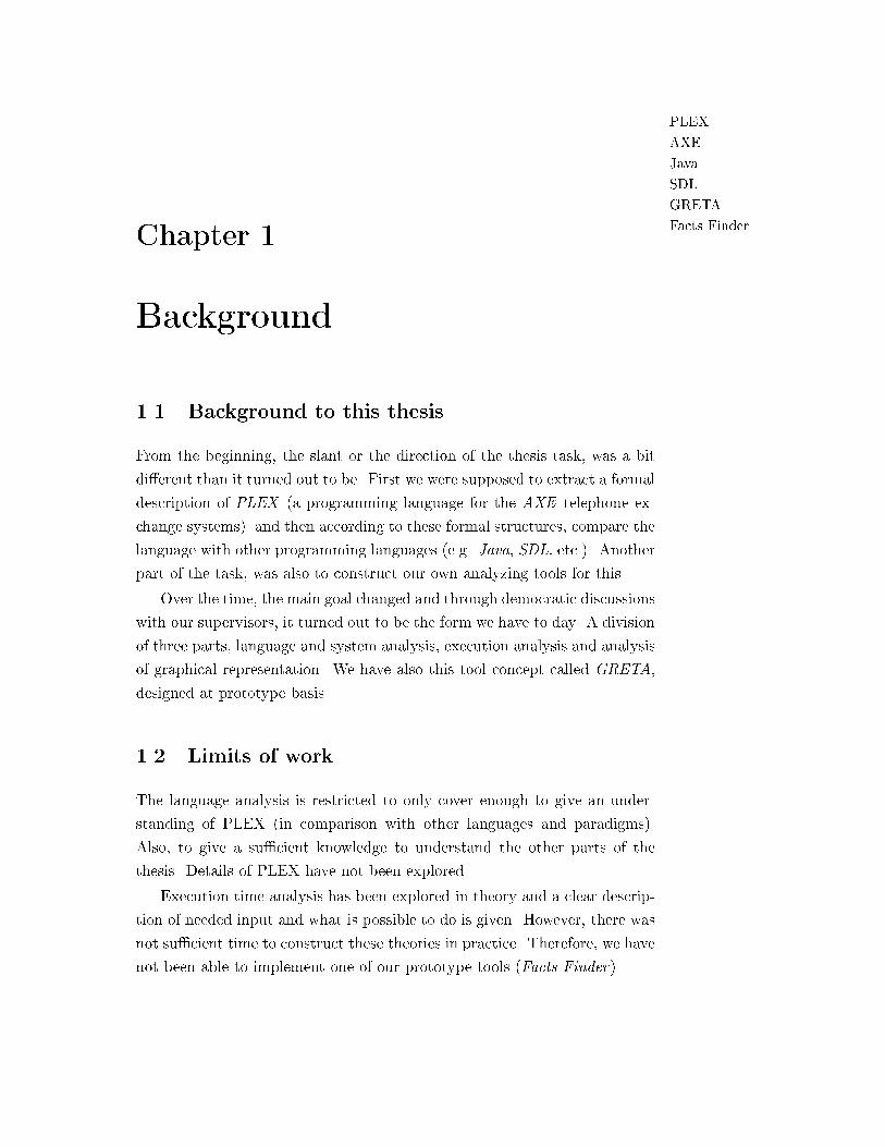
1.1 Background to this thesis
From the beginning, the slant or the direction of the thesis task, was a bit
di�erent than it turned out to be. First we were supposed to extract a formal
description of PLEX (a programming language for the AXE telephone ex-
change systems) and then according to these formal structures, compare the
language with other programming languages (e.g. Java, SDL, etc.). Another
part of the task, was also to construct our own analyzing tools for this.
Over the time, the main goal changed and through democratic discussions
with our supervisors, it turned out to be the form we have to day. A division
of three parts, language and system analysis, execution analysis and analysis
of graphical representation. We have also this tool concept called GRETA,
designed at prototype basis.
1.2 Limits of work
The language analysis is restricted to only cover enough to give an under-
standing of PLEX (in comparison with other languages and paradigms).
Also, to give a su�cient knowledge to understand the other parts of the
thesis. Details of PLEX have not been explored.
Execution time analysis has been explored in theory and a clear descrip-
tion of needed input and what is possible to do is given. However, there was
not su�cient time to construct these theories in practice. Therefore, we have
not been able to implement one of our prototype tools (Facts Finder).
2 CHAPTER 1. BACKGROUND
1.3 Read instructions
If you are not familiar with AXE and PLEX, it is probably best if you �rst
read through chapter 2. Other people can perhaps skip this.
Chapter 3 and 4 are suitable to read for you who are interested in system
and language analysis.
Chapter 5 is adequate to read for you who want to enter deeply into the
subject, execution time calculations.
If you want to learn more about graphical representation, chapter 6 may
be interesting.
Chapter 7, describes (in more detail) the prototypes in our tool concept
GRETA.
Chapter 8, is a summary of the complete thesis. For you who just want to
read the most important parts without enter deeply into details, this chapter
may be su�cient.
PLEX
AXE
Ellemtel
Televerket
Telia
SPC (Stored ProgramControl)Chapter 2
Introduction to AXE and
PLEX
2.1 The AXE system
In this chapter we are going to describe what PLEX actually is. But before
we do that we have to make a short introduction to the AXE system.
2.1.1 AXE introduction
The development of AXE started around 1972 by Ellemtel Utvecklings AB,
a company that was founded as a cooperation between L M Ericsson and
Televerket1. The AXE system was further developed during the seventies
and released as a commercial product around 1978. Today it is Ericsson
Utvecklings AB who runs the business alone without Televerket.
Basically AXE is a digital telephone exchange system which consist of
both hardware and software. Formally we call AXE a Stored Program Control
(SPC) exchange. This means, software stored in a computer to run telephone
exchange equipment.
Back in the seventies, AXE was the new invention that made it possible
to use digital instead of analog telephony. Some people claim the change
from analog to digital telephony was as big as going from farmer society
to industrialization. According to [13], the AXE system probably was the
largest development project ever made in Sweden. Perhaps, it was also the
largest stand-alone innovation.
1Televerket is nowadays known as Telia.
4 CHAPTER 2. INTRODUCTION TO AXE AND PLEX
AKE
APZ
APT
Historically the company �rst launched a system called AKE 12 before
they started with AXE. AKE worked together with an APZ processor. This
system was built on a primitive machine-oriented real-time2 model, based
on the technology at that time. The next version AKE 13, was based on the
same real-time model as AKE 12. It had a new form of a block structure,
but the AKE 13 system could not be used because it did not �t together
with the APZ processor properly. The company then had to continue with
the old AKE 12 system.
Because of the fact that both the AKE systems did not work so well
together with the APZ processor, the real-time functionality could not be
implemented. It was not until AXE 10 was introduced as a new system
(based on the APZ 210 processor) that the advantages in the block oriented
real-time model could be used.
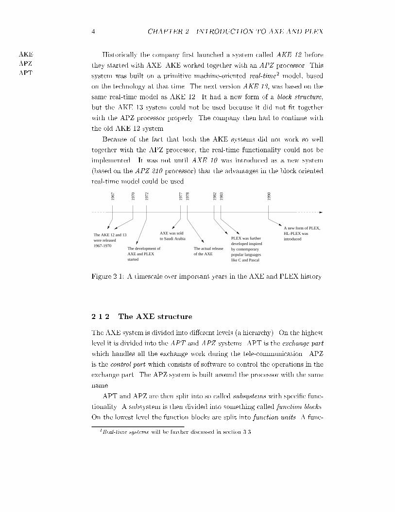
1972
1978
1982
1977
1970
1990
The actual releaseof the AXE
1967
1983
The AKE 12 and 13were released1967-1970
AXE was soldto Saudi Arabia
The development ofAXE and PLEXstarted
PLEX was furtherdeveloped inspiredby contemporarypopular languageslike C and Pascal
A new form of PLEX,HL-PLEX wasintroduced
Figure 2.1: A timescale over important years in the AXE and PLEX history.
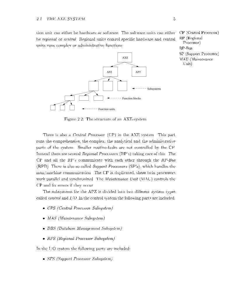
2.1.2 The AXE structure
The AXE system is divided into di�erent levels (a hierarchy). On the highest
level it is divided into the APT and APZ systems. APT is the exchange part
which handles all the exchange work during the tele-communication. APZ
is the control part which consists of software to control the operations in the
exchange part. The APZ system is built around the processor with the same
name.
APT and APZ are then split into so called subsystems with speci�c func-
tionality. A subsystem is then divided into something called function blocks.
On the lowest level the function blocks are split into function units. A func-
2Real-time systems will be further discussed in section 3.3.
2.1. THE AXE SYSTEM 5
CP (Central Processor)
RP (RegionalProcessor)
RP-Bus
SP (Support Processor)
MAU (MaintenanceUnit)
tion unit can either be hardware or software. The software units can either
be regional or central. Regional units control speci�c hardware and central
units runs complex or administrative functions.
AXE
APZ APT
Function blocks
Function units
Subsystems
Figure 2.2: The structure of an AXE-system.
There is also a Central Processor (CP) in the AXE system. This part
runs the comprehensive, the complex, the analytical and the administrative
parts of the system. Smaller routine-tasks are not controlled by the CP.
Instead there are several Regional Processors (RP's) taking care of this. The
CP and all the RP's communicate with each other through the RP-Bus
(RPB). There is also so called Support Processors (SP's), which handles the
man/machine communication. The CP is duplicated, these twin processors
work parallel and synchronized. The Maintenance Unit (MAU) controls the
CP and �x errors if they occur.
The subsystems for the APZ is divided into two di�erent system types
called control and I/O. In the control system the following parts are included:
� CPS (Central Processor Subsystem)
� MAS (Maintenance Subsystem)
� DBS (Database Management Subsystem)
� RPS (Regional Processor Subsystem)
In the I/O system the following parts are included:
� SPS (Support Processor Subsystem)
6 CHAPTER 2. INTRODUCTION TO AXE AND PLEX
PLEX
FORTRAN
Pascal
C language
HL-PLEX
real-time systems
modularity
� MCS (Man/Machine Communication Subsystem)
� FMS (File Management Subsystem)
� DCS (Data Communication Subsystem)
� OCS (Open Communication Subsystem)
2.2 The language PLEX
PLEX is a programming language which was developed by Ellemtel UAB in
the seventies parallel to the AXE system. The goal was of course to make a
programming language which was custom-made for the AXE system. If we
study the word `PLEX', we see it is an acronym for Programming Languages
for EXchanges.
2.2.1 PLEX introduction
The �rst structure of PLEX was quite inspired by the contemporary popular
programming language FORTRAN. In these years this was rather unique,
because complex embedded systems were commonly programmed in ma-
chine code. With PLEX this could be avoided and the programmer had the
possibility to develop a system in a high-level syntax.
Around 1983, PLEX was further improved. The new extensions seemed
to be highly in�uenced by other popular high-level languages at the time
(e.g. Pascal and C ).
In 1990 a new form of PLEX language was introduced, HL-PLEX. There
is a more detailed description of HL-PLEX in section 4.2
We said earlier in section 2.1.1 that the AXE system was based on a real-
time model. This can be compared to a soft real-time system. The real-time
model uses signals between function blocks and the outer world. The PLEX
code itself, is placed as signal entries in these function blocks. Real-time
systems in general are further discussed in an own section 3.3.
2.2.2 What is unique with PLEX?
PLEX code is based on a `modular structure'. This architecture makes sure
that only a single program (a program module) can manipulate some speci�c
data (a data module). Or put it this way, one module can be modi�ed
2.2. THE LANGUAGE PLEX 7
signal entry
PS (Program Store)
SDT (SignalDistribution Table)
SST (Signal SendingTable)
RS (Reference Store)
direct signals
bu�ered signals
C language
Pascal
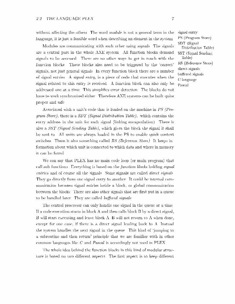
without a�ecting the others. The word module is not a general term in the
language, it is just a feasible word when describing an element in the system.
Modules are communicating with each other using signals. The signals
are a central part in the whole AXE system. All function blocks demand
signals to be accessed. There are no other ways to get in touch with the
function blocks. These blocks also need to be triggered by the `correct'
signals, not just general signals. In every function block there are a number
of signal entries. A signal entry, is a piece of code that executes when the
signal related to this entry is received. A function block can also only be
addressed one at a time. This simpli�es error detection. The blocks do not
have to work synchronized either. Therefore AXE systems can be built quite
proper and safe.
Associated with a unit's code that is loaded on the machine in PS (Pro-
gram Store), there is a SDT (Signal Distribution Table), which contains the
entry address in the unit for each signal (linking encapsulation). There is
also a SST (Signal Sending Table), which gives the block the signal it shall
be sent to. All units are always loaded in the PS to enable quick context
switches. There is also something called RS (Reference Store). It keeps in-
formation about which unit is connected to which data and where in memory
it can be found.
We can say that PLEX has no main code loop (or main program) that
call sub-functions. Everything is based on the function blocks holding signal
entries and of course all the signals. Some signals are called direct signals.
They go directly from one signal entry to another. It could be internal com-
munication between signal entries inside a block, or global communication
between the blocks. There are also other signals that are �rst put in a queue
to be handled later. They are called bu�ered signals.
The central processor can only handle one signal in the queue at a time.
If a code execution starts in block A and then calls block B by a direct signal,
B will start executing and leave block A. B will not return to A when done,
except for one case, if there is a direct signal leading back to A. Instead
the system handles the next signal in the queue. This kind of `jumping to
a subroutine and then return' principle that we are familiar with in other
common languages like C and Pascal is accordingly not used in PLEX.
The whole idea behind the function blocks in this kind of modular struc-
ture is based on two di�erent aspects. The �rst aspect is to keep di�erent
8 CHAPTER 2. INTRODUCTION TO AXE AND PLEX
EmuTool
EmuDumpGenTool
system parts isolated from each other, to avoid the single point of failure3
problem. The second aspect is modular functionality for the customers.
They can add and remove features to the system by replacing a module with
another. This makes AXE very �exible.
2.2.3 How do we run PLEX code?
Like in many other high-level languages the PLEX code is written in an
editor and then compiled into binary code. What is actually written, is the
code entries for all signals. Each block has an amount of signal code entries.
We can call them code-items. The compiled PLEX code (the binary code) is
later uploaded to the AXE hardware before delivery to the customer. The
editor and several tools for controlling the code is stored in a standard PC
or a work station. Before the code is uploaded to the AXE hardware, it has
to be tested in an APZ emulator called EmuTool. This tool emulates the
entire APZ including the central processor. EmuTool takes a binary �le, a
so called dump �le as input. This dump �le includes compiled code for all
blocks involved. EmuDumpGenTool is a program for creating dump �les.
3If the whole system is able to crash just according to errors in a single part of the
system, we can say it has the single point of failure problem.
operating system
APT
APZ
CP (Central Processor)
RP (RegionalProcessor)
multitasking
initialization signal
Chapter 3
System Analysis
3.1 Operating systems
As we said in the introduction the AXE system is divided into two main
parts. APT , the telephony or switching part and APZ , the control part.
These two domains are then split into smaller and smaller parts forming the
hierarchy we talked about in section 2.1.2. We have also claimed that the
APZ consists of a CP (Central Processor), its operating system and several
RP's (Regional Processors) with their operating systems. The CP is the
central control unit of the system and it takes all the non-trivial decisions.
The RP's perform routine operations. However, as the development goes on,
new types of regional processors have been introduced and the performance
gap between RP's and CP's is decreasing.
3.1.1 Introduction to operating systems
The operating system in the central processor has a structure of a multitask-
ing system and is mainly executed by micro programs that carry out the
internal function of the central processor. This internal function can handle
uninterrupted sequences of operations, job administrations (like signal han-
dling), signal conversion and the signal bu�er. When the system starts or
a restart is performed, the operating system sends an initialization signal ,
whose main purpose is to execute some data initialization code.
Jobs are prioritized in `level of importance'. To ensure this the micro
programs are aided by an interrupt handled system with a number of levels.
A typical structure is, a RM (Register Memory), a number of job bu�ers, a
10 CHAPTER 3. SYSTEM ANALYSIS
interrupt handledsystem
RM (Register Memory)
job bu�ers
job table and a number of time queues.
3.1.2 Interrupt handled system
An interrupt handled system works as follow. A job in progress can be
interrupted by a high-priority signal only if the signal has higher priority than
this job. In the opposite case, if a job on a high priority level is executing,
then an interrupt by a low priority signal has to wait until all jobs at higher
levels are �nished. So no interruption by a signal with the same priority is
allowed. Various registers are used to store di�erent kinds of data when a
job is running. For this reason each level is assigned a own set of registers
to avoid preserving of all data during change of level. This means exchange
of a set of registers when an interrupt is occurring. A description of existing
levels in the interrupt handled system can be found in [15].
3.1.3 Register memory
The RM is used for standardized data-transfer and addressing between the
function blocks. This register memory is located in the CP.
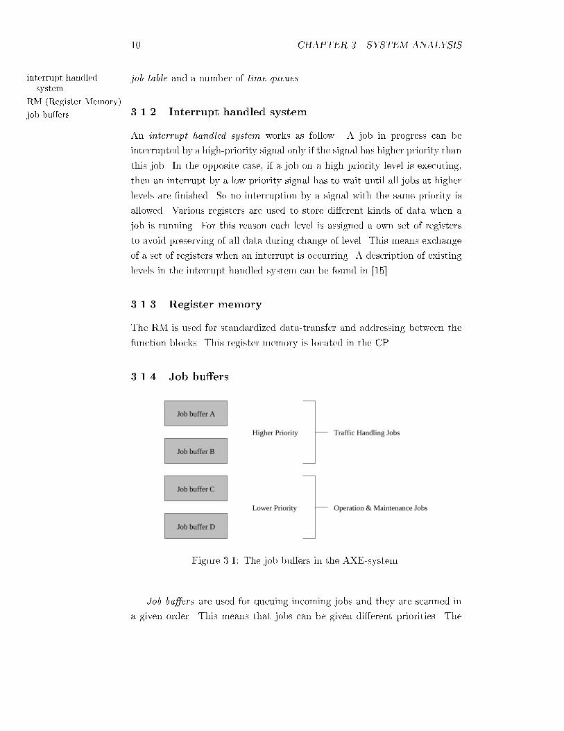
3.1.4 Job bu�ers
Job buffer A
Job buffer B
Job buffer C
Job buffer D
Higher Priority
Lower Priority
Traffic Handling Jobs
Operation & Maintenance Jobs
Figure 3.1: The job bu�ers in the AXE-system.
Job bu�ers are used for queuing incoming jobs and they are scanned in
a given order. This means that jobs can be given di�erent priorities. The
3.1. OPERATING SYSTEMS 11
direct signals
bu�ered signals
single signal
combined signal
unique signal
multiple signal
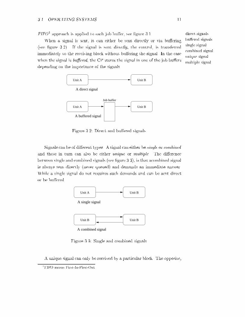
FIFO1 approach is applied to each job bu�er, see �gure 3.1.
When a signal is sent, it can either be sent directly or via bu�ering
(see �gure 3.2). If the signal is sent directly, the control, is transferred
immediately to the receiving block without bu�ering the signal. In the case
when the signal is bu�ered, the CP stores the signal in one of the job bu�ers
depending on the importance of the signals.
Unit A Unit B
Unit A Unit B
Job buffer
A buffered signal
A direct signal
Figure 3.2: Direct and bu�ered signals.
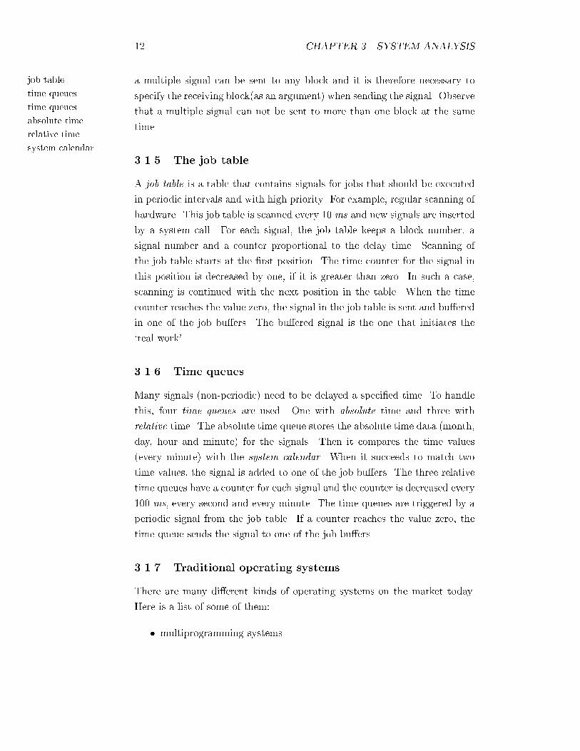
Signals can be of di�erent types. A signal can either be single or combined
and these in turn can also be either unique or multiple. The di�erence
between single and combined signals (see �gure 3.3), is that acombined signal
is always sent directly (never queued) and demands an immediate answer.
While a single signal do not requires such demands and can be sent direct
or be bu�ered.
A single signal
A combined signal
Unit A
Unit B
Unit B
Unit B
Figure 3.3: Single and combined signals.
A unique signal can only be received by a particular block. The opposite,
1FIFO means First-In-First-Out
12 CHAPTER 3. SYSTEM ANALYSIS
job table
time queues
time queues
absolute time
relative time
system calendar
a multiple signal can be sent to any block and it is therefore necessary to
specify the receiving block(as an argument) when sending the signal. Observe
that a multiple signal can not be sent to more than one block at the same
time.
3.1.5 The job table
A job table is a table that contains signals for jobs that should be executed
in periodic intervals and with high priority. For example, regular scanning of
hardware. This job table is scanned every 10 ms and new signals are inserted
by a system call. For each signal, the job table keeps a block number, a
signal number and a counter proportional to the delay time. Scanning of
the job table starts at the �rst position. The time counter for the signal in
this position is decreased by one, if it is greater than zero. In such a case,
scanning is continued with the next position in the table. When the time
counter reaches the value zero, the signal in the job table is sent and bu�ered
in one of the job bu�ers. The bu�ered signal is the one that initiates the
`real work'.
3.1.6 Time queues
Many signals (non-periodic) need to be delayed a speci�ed time. To handle
this, four time queues are used. One with absolute time and three with
relative time. The absolute time queue stores the absolute time data (month,
day, hour and minute) for the signals. Then it compares the time values
(every minute) with the system calendar. When it succeeds to match two
time values, the signal is added to one of the job bu�ers. The three relative
time queues have a counter for each signal and the counter is decreased every
100 ms, every second and every minute. The time queues are triggered by a
periodic signal from the job table. If a counter reaches the value zero, the
time queue sends the signal to one of the job bu�ers.
3.1.7 Traditional operating systems
There are many di�erent kinds of operating systems on the market today.
Here is a list of some of them:
� multiprogramming systems
3.1. OPERATING SYSTEMS 13
trap
system call
interrupt clock
time slicing
running state
block state
ready state
� multi user systems
� real-time operating systems
� timesharing systems
� single user systems
� distributed operating systems
� multiprocessor systems
Most operating systems are process based. Commonly they also have to
be organized so they can control hardware devices and applications started
by users. Occasionally, `jobs' started by users, make requests to the operating
system by a trap or a system call. These requests transfer the control from
the user to the operating system. The job is then blocked until the requested
action has been completed. Afterwards the job is released and can continue
its execution.
Operating systems usually use an interrupt clock, which sends interrupt
signals to the operating system itself. These interrupts transfer the control
from the user's job to the operating system. This means that time slicing
can be implemented to prevent that jobs are running in in�nite loops and to
encourage other users to use the CPU.
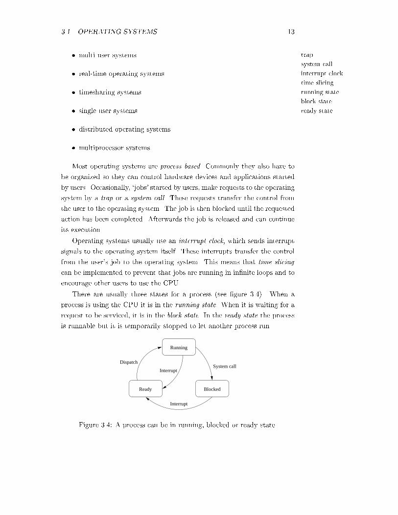
There are usually three states for a process (see �gure 3.4). When a
process is using the CPU it is in the running state. When it is waiting for a
request to be serviced, it is in the block state. In the ready state the process
is runnable but it is temporarily stopped to let another process run.
Running
BlockedReady
Dispatch
InterruptSystem call
Interrupt
Figure 3.4: A process can be in running, blocked or ready state.
14 CHAPTER 3. SYSTEM ANALYSIS
process scheduler
process table
execution e�cient
time consuming
shared memory
The process scheduler is a part of the operating system and its main
function is to decide which process should run, when and for how long. There
are many algorithms that can be used for this. The most common type, is
an algorithm that tries to balance all competing demands of e�ciency (in
the system) as a fair individual process.
When using the process model, the operating system needs a queue. This
is for maintaining of the ready-processes. We use a process table, which
contains information about each process. E.g. this information could be the
state of the process, a counter, stack pointer, memory allocation (addresses),
scheduling information and so on. When an interrupt occurs, the interrupt
service starts by saving information about the current process in the process
table. The next step is to determine which process should run next, all
according to the scheduling algorithm.
3.1.8 Execution e�cient
If we are going to compare the execution e�cient between a signal based
system (like in AXE) and a process based system, it can lead to di�erent
conclusions. This is because it depends on what scheduling algorithm we use
in the systems. At a �rst glance, a signal based system seems to be more
e�cient, if we look at the job management. In a signal based system, all
exchange of information (between software units) only take place by means
of signals. Therefore we can say that software units `sleeps' until they are
activated by a signal. Then they start to execute. The software unit itself is
the only one that has access to its own data. This private data is therefore
protected from other software units.
A signal based system is also slightly time consuming, by means of ex-
changing jobs. On the other hand, a process based system is usually even
more time consuming because it has to create, destroy and manage all the
processes. This will de�nitely decrease the execution e�cient for these sys-
tems.
3.1.9 Shared memory (semaphores)
In some operating systems, processes that are working together share some
common storage, that each process can read or write. The storage may be in
the main memory or in a shared �le. It usually takes more time for a process
to access shared memory, than to access its own private memory. This is
3.1. OPERATING SYSTEMS 15
mutual exclusion
semaphores
monitors
event counters
message counting
fault handling
MAS (MaintenanceSubsystem)
hardware faults
MAU (MaintenanceUnit)
updating duringexecution
because of the overheads associated with ensuring synchronized access. That
part of a program where the shared memory is accessed, is a critical section.
Therefore it is necessary to make sure that if one process is using a shared
variable or �le, the other processes will be excluded from using the same.
This is called mutual exclusion. For example Semaphores, monitors, event
counters, message passing etc, are used to ensure mutual exclusion.
3.1.10 Fault handling
The operating system in APZ, allows fault handling. Most errors in the soft-
ware are detected by di�erent supervision functions in MAS (Maintenance
Subsystem). These functions may result in a system restart, which will lo-
cate and repair the error. APZ will keep on running even if there are one or
more faults detected in the system.
Hardware faults may cause faults in the central processor. Generally
spoken we can say that there are two types of hardware faults. Temporary
and permanent faults. Therefore the central processor is duplicated and
these two parts work parallel in synchronous mode. One of the processors
is the standby side and the other is the executive side. The unit called the
MAU (Maintenance Unit) supervises the operation of the central processor
and takes appropriate action if faults occur. If the central processor detects
a temporary fault, it halts the a�ected side and performs a full diagnosis
of the halted side. If the error cannot be re-detected, the fault is logged
as temporary and the central processor status is set to normal. If the fault
detected is a permanent fault, the central processor cannot be put back into
normal operation. Instead an alarm is issued. AMU/MAU then tests both
sides to determine on which side the fault has occurred. The erroneous side
is then halted and both sides change places.
3.1.11 Updating during execution
A block, in the APZ system, can be updated during execution. This is very
powerful for systems that require working in all situations. A block can
be separately compiled and loaded to the system. Most traditional systems
require to be restarted when updating a part in the system. This procedure
can be time consuming and lose of system accessibility.
16 CHAPTER 3. SYSTEM ANALYSIS
system load
system clock
time accuracy
UNIX
MS-DOS
Windows
3.1.12 System load
For process based systems, the system load is depending on what schedule
algorithm is used.
The availability in the APZ is generally said to be linear to the system
load. The context switch in the APZ is insigni�cant comparing to most
process based systems. Therefore, the availability in the APZ di�ers from
the availability in some process based systems.
3.1.13 System clock
The system clock contains the absolute time of the system with year, day,
hour, minute and second. It also contains a calendar function, giving infor-
mation about the current day, about holidays and so on. A special executive
program administrates the system clock and it is not overwritten during big
system restarts. The system can be provided with an external clock refer-
ence, when high time accuracy is needed.
3.2 Signal and process based systems
Many operating systems today are process based systems like UNIX , MS-
DOS and Windows. But Ericsson's telecommunication system uses a signal
based system. In the following two sections these two concepts are explained
in more detail.
3.2.1 Signal based systems
A signal is used to perform communication between software units and it is
similar to a jump from one program (or function unit) to another.
A signal can be described as a message within one or between two soft-
ware units, or as an asynchronous (one way) function call. This means that
a unit that is executing, can end by a signal and let another unit use the
processor.
This signal paradigm is used in the APZ, the control part of the AXE.
Every signal here has its own signal description, which de�nes the number
of signal data, type and purpose of the signal etc. The signal descriptions
are stored in special libraries and are accessible through a signal-handling
database.
3.2. SIGNAL AND PROCESS BASED SYSTEMS 17
RP-CP signal
CP-CP signal
RP-RP signals
process
executable program
stack pointer
registers
handling processes
timesharing system
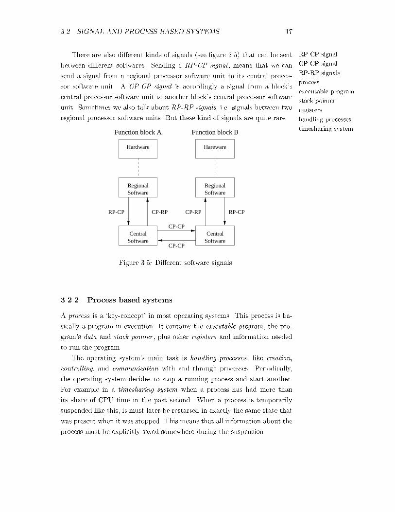
There are also di�erent kinds of signals (see �gure 3.5) that can be sent
between di�erent softwares. Sending a RP-CP signal , means that we can
send a signal from a regional processor software unit to its central proces-
sor software unit. A CP-CP signal is accordingly a signal from a block's
central processor software unit to another block's central processor software
unit. Sometimes we also talk about RP-RP signals, i.e. signals between two
regional processor software units. But these kind of signals are quite rare.
RegionalSoftware
Hardware Hareware
RegionalSoftware
CentralSoftware Software
Function block BFunction block A
CP-RP CP-RPRP-CP
CP-CP
CP-CP
RP-CP
Central
Figure 3.5: Di�erent software signals.
3.2.2 Process based systems
A process is a `key-concept' in most operating systems. This process is ba-
sically a program in execution. It contains the executable program, the pro-
gram's data and stack pointer , plus other registers and information needed
to run the program.
The operating system's main task is handling processes, like creation,
controlling, and communication with and through processes. Periodically,
the operating system decides to stop a running process and start another.
For example in a timesharing system when a process has had more than
its share of CPU time in the past second. When a process is temporarily
suspended like this, it must later be restarted in exactly the same state that
was present when it was stopped. This means that all information about the
process must be explicitly saved somewhere during the suspension.
18 CHAPTER 3. SYSTEM ANALYSIS
process table
child processes
process tree structure
overhead
In many operating systems, all the information about each process, other
than the contents of its own address space, is stored in an operating system
table called the process table. This process table is either an array or a
linked list of structures (one structure link for each process currently in
existence). The key-process management system-calls are those that handles
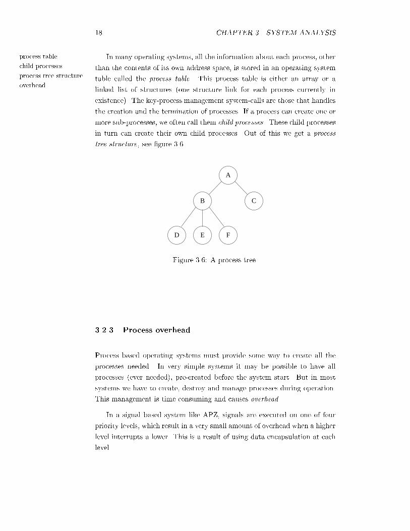
the creation and the termination of processes. If a process can create one or
more sub-processes, we often call them child processes. These child processes
in turn can create their own child processes. Out of this we get a process
tree structure, see �gure 3.6.
A
CB
D E F
Figure 3.6: A process tree.
3.2.3 Process overhead
Process based operating systems must provide some way to create all the
processes needed. In very simple systems it may be possible to have all
processes (ever needed), pre-created before the system start. But in most
systems we have to create, destroy and manage processes during operation.
This management is time consuming and causes overhead.
In a signal based system like APZ, signals are executed on one of four
priority levels, which result in a very small amount of overhead when a higher
level interrupts a lower. This is a result of using data encapsulation at each
level.
3.3. REAL-TIME SYSTEMS 19
real-time systems
average response time
time constraints
soft real-time system
hard real-time system
event triggered
3.3 Real-time systems
3.3.1 Introduction to real-time systems
A real-time system is a system that reacts on outer events read by some
kind of sensors. It also runs functions based on these events and gives the
system an answer during a determined period of time. A correct function
in a real-time system is not only based on a function giving a correct result,
the time when the result is produced is also important.
Many people think that a real-time system is the same as a `fast system'
but this is wrong. The dimension of time is totally up to the system. Some
functions may answer in a few seconds, other in a couple of micro seconds.
It is the running process (the task) that decide the dimension of time. The
goal with a `fast system' is to shorten the average response time, while the
goal with a real-time system is to ful�ll the predetermined time constraints.
3.3.2 Hard and soft real-time systems
In real-time systems we usually talk about two di�erent timing constraints,
hard and soft. Therefore we also use the terms hard real-time system and
soft real-time system.
Tasks with hard timing constraints are critical and have to be completed
before their deadline. A good example of such a task is the activation of an
airbag in a car. When a car crashes, the time until the airbag is activated is
very critical. Such things have to be completed before the deadline, else it can
damage the system itself or lead to terrible consequences in the environment.
In this airbag example, a human can die if the system fails. Therefore hard
real-time systems are often mounted in modern cars today.
Soft constraints are implemented to get the real-time system run smooth,
but they are not critical as hard constraints. In a typical soft system, a
task can miss its deadline without leading to such terrible consequences.
An example of a soft real-time system is a telephone exchange system (e.g.
AXE).
3.3.3 The real-time model in PLEX
In PLEX we have an event triggered system. We can call this a soft real-time
system. The system is designed to run smooth in the average (normal) case.
20 CHAPTER 3. SYSTEM ANALYSIS
timeout value
agent based systems
AI (Arti�cialIntelligence)
Now and then, statistics are collected and delivered to the programmers.
These statistics give the programmers knowledge about which cases that
take time. Therefore soft deadlines can be set (based on these statistics).
This is normally done by setting timeouts2 on some functions.
Sometimes, if an AXE system has to deal with really heavy tra�c, it
may crash because everything is based on statistics of a system running in
the normal case. We can put it this way, sometimes the AXE system can
`miss a deadline'. This is why we must call it a `soft system'.
3.4 Agent based systems
In Arti�cial Intelligence we often talk about systems built upon intelligent
agents. In this section we are going to describe what agents actually are and
how they possibly can be connected to an AXE structure. We are also going
to compare agents with the objects in an object oriented design.
3.4.1 Introduction to agents
An agent is like an object that have its own methods and data storage. It can
also make its own decisions, i.e. what methods that should run in di�erent
circumstances. When we construct an agent, we create a number of logical
rules that the agent has to follow. Then the agent base all decisions on these
rules when running. We can say an agent has its own life. It is not controlled
by a system on a higher level. So in an agent based system we have a number
of agents communicating with each other according to logical rules. There
is no control system that has to give orders to the agents. They can act on
their own.
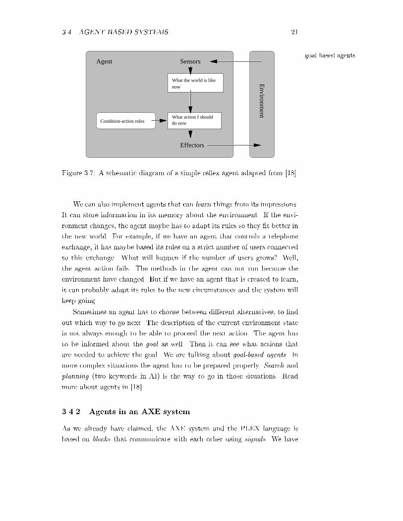
But how is it possible for an agent to make its own decisions? Well, agents
are equipped with sensors. Information in the environment can be picked
up by an agent and analyzed. All decisions are then based on what input
the agent has received. We can construct agents that receive everything
as input, or we can adapt them for just collecting subsets of information.
We can also create agents that take care of all impressions, or we can just
construct methods for some of the input.
2We can have a counter which reacts in some way when a special number (a timeout
value) is reached.
3.4. AGENT BASED SYSTEMS 21
goal-based agents
What the world is likenow
SensorsAgent
Environm
ent
Condition-action rulesWhat action I shoulddo now
Effectors
Figure 3.7: A schematic diagram of a simple re�ex agent adapted from [18].
We can also implement agents that can learn things from its impressions.
It can store information in its memory about the environment. If the envi-
ronment changes, the agent maybe has to adapt its rules so they �t better in
the new world. For example, if we have an agent that controls a telephone
exchange, it has maybe based its rules on a strict number of users connected
to this exchange. What will happen if the number of users grows? Well,
the agent action fails. The methods in the agent can not run because the
environment have changed. But if we have an agent that is created to learn,
it can probably adapt its rules to the new circumstances and the system will
keep going.
Sometimes an agent has to choose between di�erent alternatives, to �nd
out which way to go next. The description of the current environment state
is not always enough to be able to proceed the next action. The agent has
to be informed about the goal as well. Then it can see what actions that
are needed to achieve the goal. We are talking about goal-based agents. In
more complex situations the agent has to be prepared properly. Search and
planning (two keywords in AI) is the way to go in those situations. Read
more about agents in [18].
3.4.2 Agents in an AXE system
As we already have claimed, the AXE system and the PLEX language is
based on blocks that communicate with each other using signals. We have
22 CHAPTER 3. SYSTEM ANALYSIS
object oriented system also said that all signals, that can be sent from a block, are represented as
code-entries. Perhaps it is possible to transform this structure into an agent
based system. One approach is that the agents represent the blocks and the
methods in the agent represent the signals. Now we have the possibility
of creating logical rules for our `block-agents'. We can tell exactly how the
system should act in di�erent situations. So we construct an intelligent AXE
system that controls itself. The blocks would be like living objects, that can
act on their own.
Maybe it is also possible to implement the `ability to learn' in this agent
system. Then the AXE system can update itself and adapt the structure to
the environment. PLEX programmers do not have to waste their energy on
making run-time updates, they can instead concentrate on development of
the system.
3.4.3 Agents and object oriented design
When we are comparing an agent based system with an object oriented sys-
tem, we may �rst �nd them quite similar. But there are big di�erences, the
logical rules and the ability to learn. Both systems are built upon embedded
objects, but an agent can also make its own decisions during run-time. The
decisions are based on what have been seen in the environment. Agents can
also learn from mistakes, if the learning concept is implemented. Objects in
object oriented environments can run methods, but not based on own deci-
sions. Another object have to ask for the method �rst. We can say agents
`have eyes' while objects in an object oriented design are `blind'.
Chapter 4
Language Analysis
4.1 PLEX and traditional programming
4.1.1 Programming language paradigms
If we are going to compare PLEX with other traditional programming lan-
guages, it is good to �rst make an overview of the language elements. The
Fourth generationLanguage
AssemblyLanguage
Object orientedLanguage
ImperativeLanguage
ConstraintLanguage
Language
Specification
QueryLanguage
LanguageConcurrent
LanguageMeta
Single assignmentLanguage
DataflowLanguage
LanguageIntermediate
Event triggeredLanguage
LanguagesProgramming
The Paradigms ofLanguageDeclarative
LanguageDefinitional
LanguageFunctional
LanguageLogical
ProceduralLanguage
LanguageApplicative
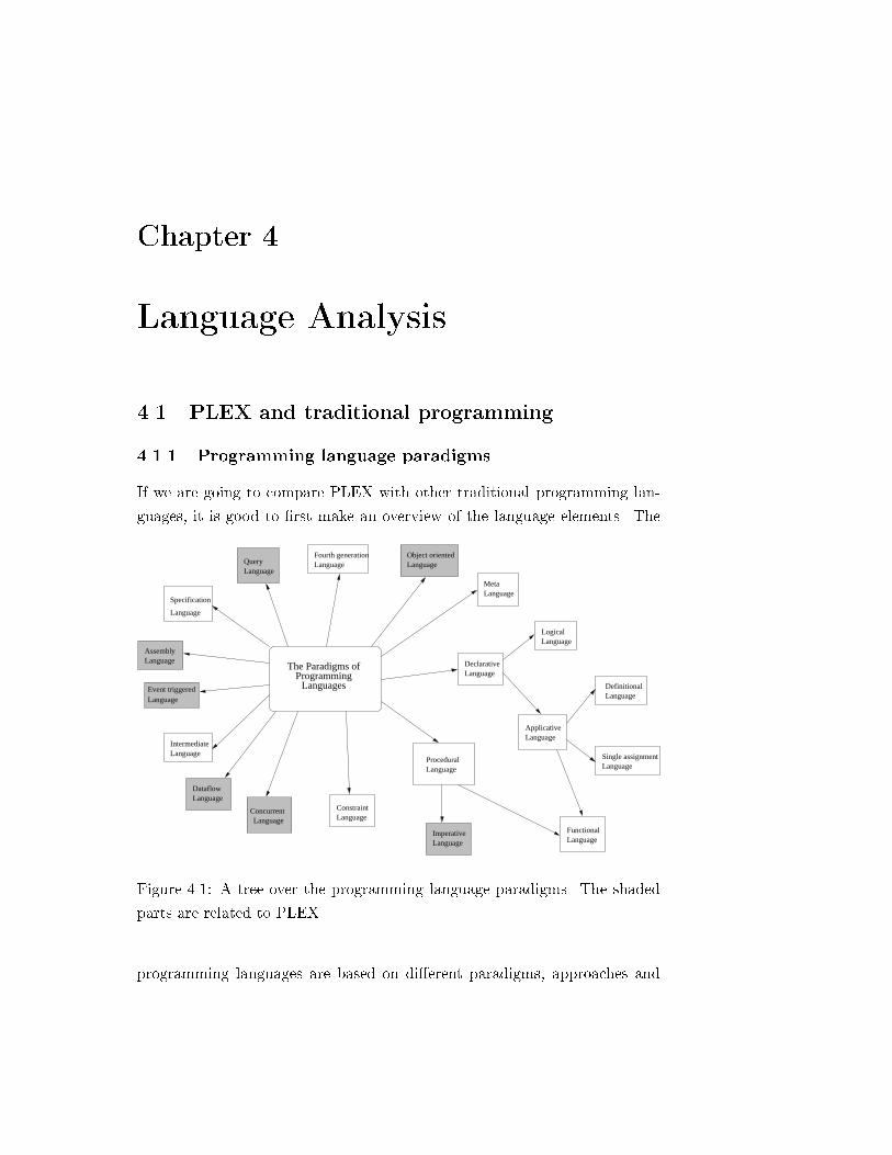
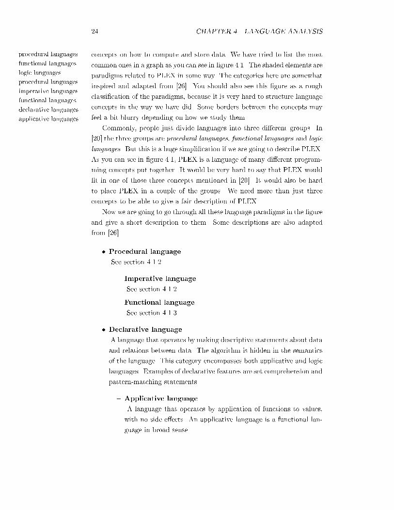
Figure 4.1: A tree over the programming language paradigms. The shaded
parts are related to PLEX.
programming languages are based on di�erent paradigms, approaches and
24 CHAPTER 4. LANGUAGE ANALYSIS
procedural languages
functional languages
logic languages
procedural languages
imperative languages
functional languages
declarative languages
applicative languages
concepts on how to compute and store data. We have tried to list the most
common ones in a graph as you can see in �gure 4.1. The shaded elements are
paradigms related to PLEX in some way. The categories here are somewhat
inspired and adapted from [26]. You should also see this �gure as a rough
classi�cation of the paradigms, because it is very hard to structure language
concepts in the way we have did. Some borders between the concepts may
feel a bit blurry depending on how we study them.
Commonly, people just divide languages into three di�erent groups. In
[20] the three groups are procedural languages, functional languages and logic
languages. But this is a huge simpli�cation if we are going to describe PLEX.
As you can see in �gure 4.1, PLEX is a language of many di�erent program-
ming concepts put together. It would be very hard to say that PLEX would
�t in one of those three concepts mentioned in [20]. It would also be hard
to place PLEX in a couple of the groups. We need more than just three
concepts to be able to give a fair description of PLEX.
Now we are going to go through all these language paradigms in the �gure
and give a short description to them. Some descriptions are also adapted
from [26].
� Procedural language
See section 4.1.2.
� Imperative language
See section 4.1.2.
� Functional language
See section 4.1.3.
� Declarative language
A language that operates by making descriptive statements about data
and relations between data. The algorithm is hidden in the semantics
of the language. This category encompasses both applicative and logic
languages. Examples of declarative features are set comprehension and
pattern-matching statements.
� Applicative language
A language that operates by application of functions to values,
with no side e�ects. An applicative language is a functional lan-
guage in broad sense.
4.1. PLEX AND TRADITIONAL PROGRAMMING 25
de�nitional languages
Lucid
GCLA
single assignmentlanguages
functional languages
logic languages
constraint languages
concurrent languages
data�ow languages
VAL
intermediate languages
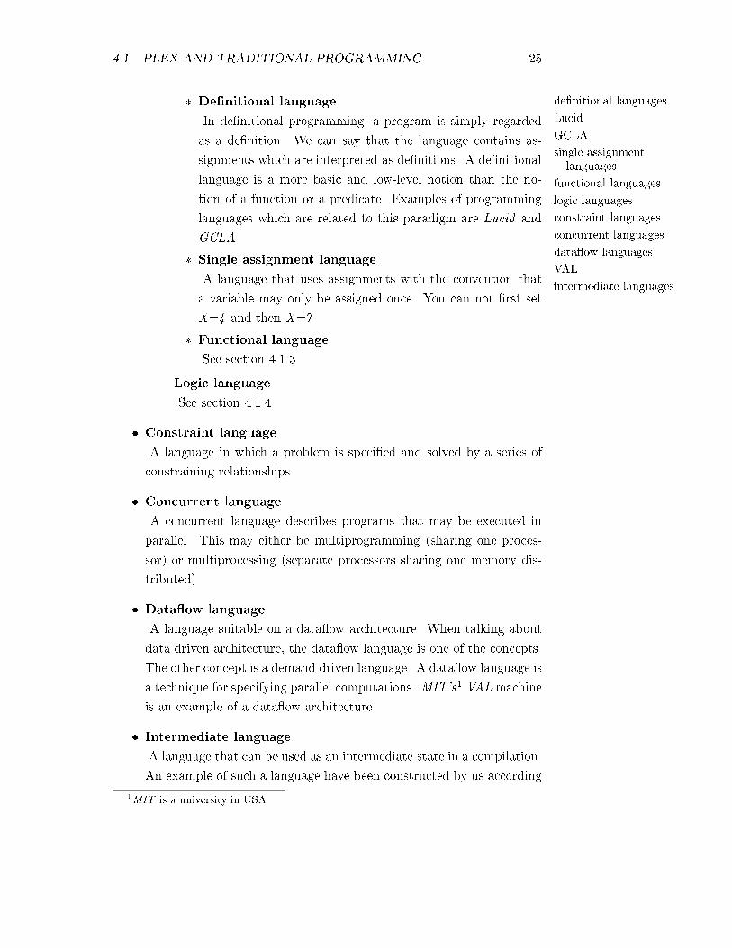
� De�nitional language
In de�nitional programming, a program is simply regarded
as a de�nition. We can say that the language contains as-
signments which are interpreted as de�nitions. A de�nitional
language is a more basic and low-level notion than the no-
tion of a function or a predicate. Examples of programming
languages which are related to this paradigm are Lucid and
GCLA.
� Single assignment language
A language that uses assignments with the convention that
a variable may only be assigned once. You can not �rst set
X=4 and then X=7.
� Functional language
See section 4.1.3.
� Logic language
See section 4.1.4.
� Constraint language
A language in which a problem is speci�ed and solved by a series of
constraining relationships.
� Concurrent language
A concurrent language describes programs that may be executed in
parallel. This may either be multiprogramming (sharing one proces-
sor) or multiprocessing (separate processors sharing one memory dis-
tributed).
� Data�ow language
A language suitable on a data�ow architecture. When talking about
data driven architecture, the data�ow language is one of the concepts.
The other concept is a demand driven language. A data�ow language is
a technique for specifying parallel computations. MIT's1 VALmachine
is an example of a data�ow architecture.
� Intermediate language
A language that can be used as an intermediate state in a compilation.
An example of such a language have been constructed by us according
1MIT is a university in USA.
26 CHAPTER 4. LANGUAGE ANALYSIS
event triggeredlanguages
assembly languages
speci�cation languages
query languages
fourth generationlanguages
4GL
object orientedlanguages
meta languages
procedural languages
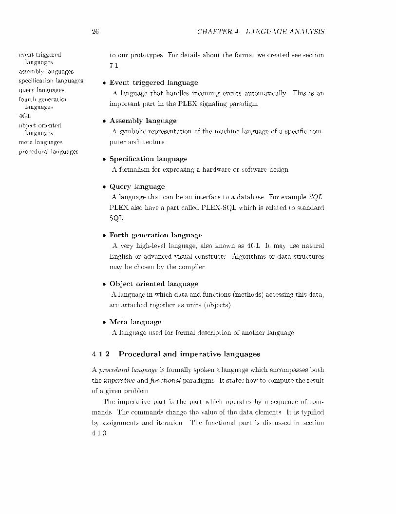
to our prototypes. For details about the format we created see section
7.1
� Event triggered language
A language that handles incoming events automatically. This is an
important part in the PLEX signaling paradigm.
� Assembly language
A symbolic representation of the machine language of a speci�c com-
puter architecture.
� Speci�cation language
A formalism for expressing a hardware or software design.
� Query language
A language that can be an interface to a database. For example SQL.
PLEX also have a part called PLEX-SQL which is related to standard
SQL.
� Forth generation language
A very high-level language, also known as 4GL. It may use natural
English or advanced visual constructs. Algorithms or data structures
may be chosen by the compiler.
� Object oriented language
A language in which data and functions (methods) accessing this data,
are attached together as units (objects).
� Meta language
A language used for formal description of another language.
4.1.2 Procedural and imperative languages
A procedural language is formally spoken a language which encompasses both
the imperative and functional paradigms. It states how to compute the result
of a given problem.
The imperative part is the part which operates by a sequence of com-
mands. The commands change the value of the data elements. It is typi�ed
by assignments and iteration. The functional part is discussed in section
4.1.3.
4.1. PLEX AND TRADITIONAL PROGRAMMING 27
C language
Pascal
FORTRAN
ADA
GOTO-command
functional languages
LISP
ML
FP
Haskell
Erlang
Less formally we can say that in procedural languages, the code is split
into a data part and a part of instructions. These instructions are then
divided into procedures, functions and subroutines. Some examples of pro-
cedural languages are C, Pascal, FORTRAN and ADA.
The structure of the PLEX code is quite related to this kind of program-
ming structure. At least the imperative part. Over the years, PLEX has also
been developed in a way to more look like C and Pascal code. CASE- and
IF-statements have been included for example. The early PLEX was more
related to FORTRAN, with the classical GOTO/LABEL-structure.
In C-programming, GOTO's are possible, but they are rarely used. Many
C-programmers think they are obsolete and `a bad thing' that makes the
code unstructured. The GOTO-command also make it harder to follow the
program �ow, than a code structured into procedures and functions.
4.1.3 Functional languages
In a functional language, everything is built upon functions. From small
primitive functions, to more advanced functions based on the primitive ones.
Typical languages are LISP, ML, FP, Haskell and Erlang.
Traditionally, functional languages do not have variables. Everything is
expressed with functions and arguments to the functions. In LISP all data is
based on lists and atoms. An atom can be a symbol, a string or a boolean2
value. Lists can either be empty, hold atoms, or hold other lists. You can
always insert atoms or lists via arguments to a function. This function
will also always return something. It may visit other functions during the
execution. But the internal function-calls will always exit sometime and
return to this main function which also �nally exits.
We can symbolize a functional program like the structure of the `Russian
wooden dolls'. This is maybe a quite blurry description but it should just be
seen as a metaphor. First we have a big doll, inside this there is a smaller
doll, and inside this there is an even smaller doll... and so on. We execute
the program by opening the dolls (the functions) until we reach the smallest
(the most primitive function). Then all functions must exit. We reconstruct
the doll again by placing a smaller doll inside a bigger until we reach the
largest one. The program ends and we get our output. Every doll here is a
function that must exit. The size of the doll in this example represent the
2A boolean value, is a value that is either true or false.
28 CHAPTER 4. LANGUAGE ANALYSIS
logic languages
Prolog
backtracking
triviality of function. The largest doll is on the highest level, `closest to the
user'. The smallest doll is on the lowest level, the most primitive function,
`closest to the computer'.
As we already have said, this doll example should just be seen as a
metaphor or a simpli�cation of what a functional structure can look like
in theory. In LISP, functions can also of course include more than one
single function call inside each function. The main aspect is though that
all functions return values. If no special return expressions are speci�ed,
functions in LISP return true or false. This boolean value depends on the
success of running the function.
4.1.4 Logic languages
In a logic and declarative language like Prolog, you are working with pred-
icates and relationships, i.e. p(X,Y). Everything is based on three kinds of
horn clauses, facts, logical rules and queries. You de�ne all valid rules.
Facts can be like p(john,10), which means that it is true that john and
10 has some kind of a relation. Rules can be seen as functions based on the
facts. It could be like p is true if f1, f2, f3... are true.
This kind of rule based representation enables analysis and it is possi-
ble to ask questions (queries) and let the program �nd solutions based on
the logical rules. This kind of programming is very often used in Arti�cial
Intelligence.
We could express all the signals in a PLEX system as logical rules (an
abstraction of the selected blocks). This would enable di�erent forms of
logical analysis's of the signal �ow. If we construct a program that translates
all signal rules into logical rules, e.g. `Block A has signal S1', `Signal S2 leads
to block B' and so on. This would also make it possible to ask questions
like, `Which signals are connected to block A?', `Has block A and block B a
connection?' and `Can signal S1 occur directly after signal S2?'.
In Prolog all possible solutions could be generated and listed. If the
system gets stuck on a branch in the search tree, it will automatically step
back and try another way. This process when the program steps back is
called backtracking in Prolog. So all solutions will always be found if there
are any. This is believed to be a feasible approach to analyze systems written
in PLEX. In one of our prototypes, we have used Prolog for such a purpose.
For more details see section 7.3.
4.2. HL-PLEX 29
HL-PLEX
C language
Pascal
4.2 HL-PLEX
4.2.1 Introduction to HL-PLEX
One of the major goals for Ericsson UAB is to reduce the number of coding
faults. Instead of searching for errors, the company of course want to con-
centrate on development of new functionality in the AXE system. Therefore
a new form of programming language was founded in 1990-91. It was called
HL-PLEX, which is an abbreviation for High Level Programming Language
for EXchanges. The new language was designed to produce well structured,
easy read, high quality code, which also should be modular and reusable.
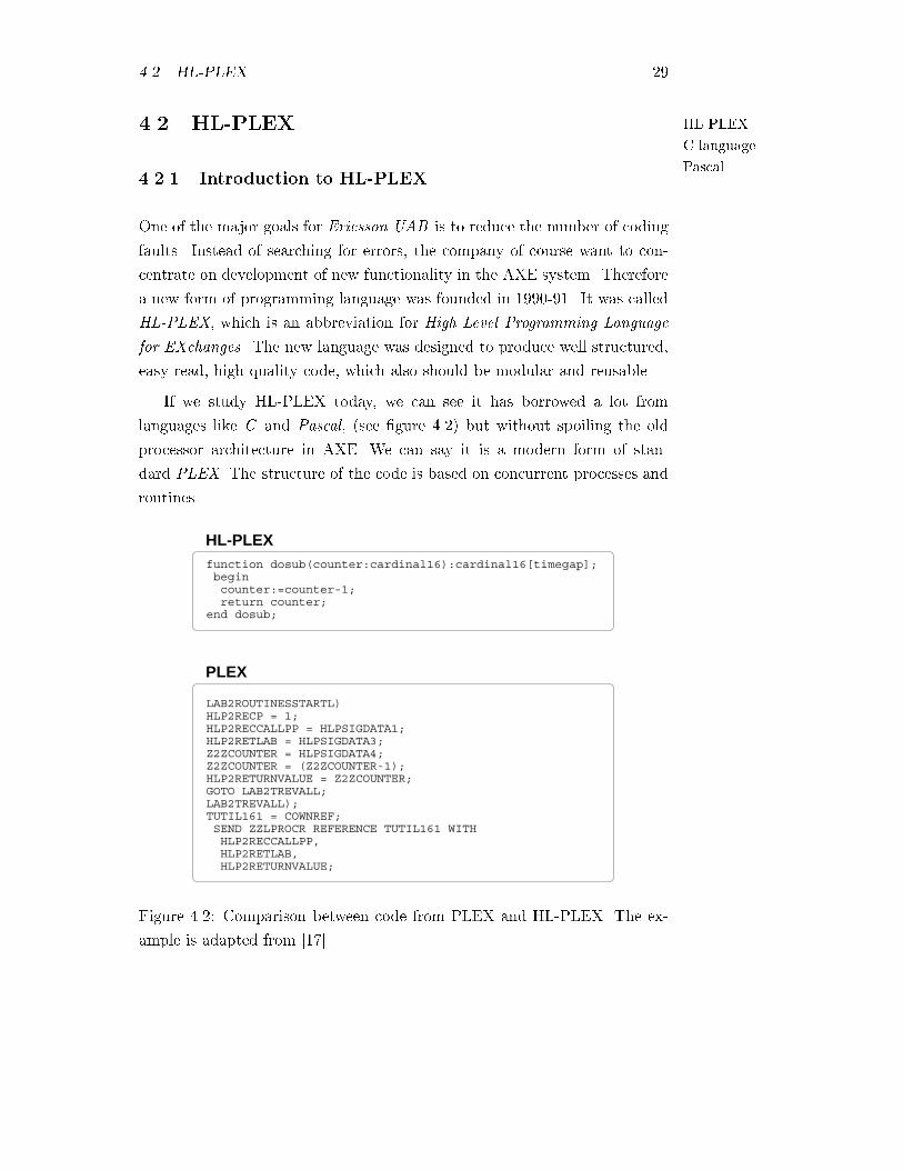
If we study HL-PLEX today, we can see it has borrowed a lot from
languages like C and Pascal, (see �gure 4.2) but without spoiling the old
processor architecture in AXE. We can say it is a modern form of stan-
dard PLEX. The structure of the code is based on concurrent processes and
routines.
function dosub(counter:cardinal16):cardinal16[timegap]; begin counter:=counter-1; return counter; end dosub;
LAB2ROUTINESSTARTL) HLP2RECP = 1; HLP2RECCALLPP = HLPSIGDATA1; HLP2RETLAB = HLPSIGDATA3; Z2ZCOUNTER = HLPSIGDATA4; Z2ZCOUNTER = (Z2ZCOUNTER-1); HLP2RETURNVALUE = Z2ZCOUNTER;
LAB2TREVALL); TUTIL161 = COWNREF; SEND ZZLPROCR REFERENCE TUTIL161 WITH HLP2RECCALLPP, HLP2RETLAB, HLP2RETURNVALUE;
GOTO LAB2TREVALL;
PLEX
HL-PLEX
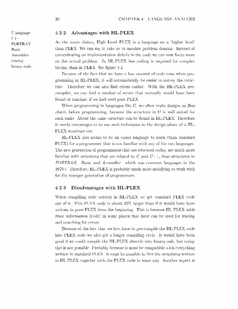
Figure 4.2: Comparison between code from PLEX and HL-PLEX. The ex-
ample is adapted from [17].
30 CHAPTER 4. LANGUAGE ANALYSIS
C language
C++
FORTRAN
Basic
Assembler
tracing
binary code
4.2.2 Advantages with HL-PLEX
As the name claims, High Level PLEX is a language on a `higher level'
than PLEX. We can say it take us to another problem domain. Instead of
concentrating on implementation details in the code we can now focus more
on the actual problem. In HL-PLEX less coding is required for complex
blocks, than in PLEX. See �gure 4.2.
Because of the fact that we have a less amount of code rows when pro-
gramming in HL-PLEX, it will automatically be easier to survey the struc-
ture. Therefore we can also �nd errors earlier. With the HL-PLEX pre-
compiler, we can �nd a number of errors that normally would have been
found at runtime, if we had used pure PLEX.
When programming in languages like C, we often make designs as �ow
charts before programming, because the structure in C is well suited for
such tasks. About the same structure can be found in HL-PLEX. Therefore
it surely encourages us to use such techniques in the design phase of a HL-
PLEX structure too.
HL-PLEX also seems to be an easier language to learn (than standard
PLEX) for a programmer that is not familiar with any of the two languages.
The new generation of programmers that are educated today, are much more
familiar with structures that are related to C and C++, than structures in
FORTRAN, Basic and Assembler which was common languages in the
1970's. Therefore, HL-PLEX is probably much more satisfying to work with
for the younger generation of programmers.
4.2.3 Disadvantages with HL-PLEX
When compiling code written in HL-PLEX we get standard PLEX code
out of it. This PLEX code is about 20% larger than if it would have been
written in pure PLEX from the beginning. This is because HL-PLEX adds
trace information (code) in some places that later can be used for tracing
and searching for errors.
Because of the fact that we �rst have to pre-compile the HL-PLEX code
into PLEX code we also get a longer compiling cycle. It would have been
good if we could compile the HL-PLEX directly into binary code, but today
this is not possible. Probably because it must be compatible with everything
written in standard PLEX. It must be possible to link the structures written
in HL-PLEX together with the PLEX code in some way. Another aspect is
4.2. HL-PLEX 31
pre-compiler
optimization
also that it cost a lot to develop a new compiler that can turn HL-PLEX
code directly to binary code.
Another drawback with HL-PLEX is that the PLEX-code, constructed
by the pre-compiler, maybe is not optimized enough. The compiler optimizes
everything automatically using built-in algorithms. It will probably generate
quite good PLEX code, but it will also be a bit di�erent to a code written
manually by a human. An experienced person who has written code in
standard PLEX for many years, maybe write much more optimized code
than what is generated automatically by the HL-PLEX pre-compiler.
execution timecalculation
low-level analysis
worst case behavior
high-level analysis
false paths
Chapter 5
Execution Time Calculation
5.1 Introduction to execution time calculation
If we are able to estimate or calculate the execution time for a piece of code we
can get good knowledge about its capability. This can be important in both
hard and soft real-time systems. As we said in section 3.3.3 the AXE-system
is a soft real-time system and execution time calculation is useful information
when analyzing PLEX. It will aid programmers in meeting requirements by
producing better implementations, modi�cations and optimizations.
5.1.1 Current research
In the current research of execution time calculation there are mainly two
approaches of calculating the time of tasks. The �rst approach is to make a
low-level analysis. This is done by modeling the behavior of the hardware and
then by various optimization techniques try to �nd the worst case behavior.
Another way is to make a high-level analysis. This is a semantic analysis
where we try to �nd such things like false paths and overestimations of loop
counts in the code.
Both these two approaches are interesting and to combine them is prob-
ably even more interesting. A method called Integer Linear Programming
(ILP) does this. For further details of ILP see [7].
5.1. INTRODUCTION TO EXECUTION TIME CALCULATION 33
ILP (Integer LinearProgramming)
�ow graph
WCET (Worst CaseExecution Time)
WCETc (Worst CaseExecution Timecalculation)
Mälardalen University
5.1.2 ILP, a method for execution time calculation
In the ILP method we �rst transform the program code into a �ow graph.
The �ow graph consists of nodes and edges. A node is a basic code block,
one single instruction or some instructions collected together. Each edge
represent theWCET (Worst Case Execution Time), which is calculated from
the instructions in the block (the node). The total execution time of the
whole �ow graph is shown as a so called linear expression. Then a WCETc
(Worst Case Execution Time calculation) is done to �nd the maximum of
the expression.
5.1.3 Tools for execution time calculation
Today there are no commercial tools available for calculating execution times
of code. A few companies around the world probably have invented their
own tools for this purpose. In spring 1997 an investigation was made among
Nordic companies to �nd out more about the problem of determining execu-
tion times. The following result have been summarized by Jan Gustafsson
in [6] at Mälardalen University , Sweden, in 1997:
About 50 companies answered. 70% were analyzing execution times on
a regular basis. 94% wanted to have a tool for calculating execution time.
90% wanted input data dependent calculations.
� The methods that were used was:
emulators, simulators, measuring with logic analyzer, measuring with
oscilloscope and port addressings, measuring with entered timer calls,
manually calculate the assembler instructions and �nally pro�ler tools.
� The typical analyzed programs were:
small assembler programs, critical code sections, time-critical applica-
tions, interrupt routines, DSP-programs in assembler.
� The four main reasons to analyze the execution times were:
To ful�ll the real-time requirements, to optimize the code, to compare
algorithms, to evaluate hardware.
34 CHAPTER 5. EXECUTION TIME CALCULATION
calculate executiontime
low-level analysis
high-level analysis
assembler code
5.2 Problems with execution time calculation
When we need to know the total execution time for a given job there are a
few problems that has to be solved. First how the actual calculation is done
and then how to handle loops.
5.2.1 How to calculate the execution time?
As we said in 5.1.1, there are two main approaches when calculating execu-
tion times. The low-level analysis and the high-level analysis.
Low-level analysis
In the low-level analysis we try to model the behavior of the system (or a part
of it) and then according to that behavior we try to calculate the execution
time. The analysis is done on low-level, which means that the object code or
the assembler code is analyzed. Analyzing assembler code is to look up each
assembler instruction in a table where the execution time (clock ticks) for
each instruction is given. These time values di�er according to the processor-
type and therefore we need to do the execution time calculation for a given
processor. Further, to be able to analyze on a low-level, we need to have
the system (or a part of it) compiled and linked. This is because we need
the object code or the assembler code, but also because the AXE system
is undecidable before compilation and linking. It is �rst in the compiled
and linked system we know which code will be executed for a given signal.
Knowing exactly which code will be executed next is necessary input to the
execution time calculation, as we need to know the �ow (see section 5.2.4)
of the program.
It is preferred to calculate the execution time in a stage before the whole
system is up and running. Calculating execution times is a step that we want
to use as soon as possible in the developing process. An early estimation of
the execution time can speed up the process as it will be easier to correct
mistakes. It can also help to clean up the code, because it is possible to see
that some steps take too much time.
High-level analysis
In the high-level analysis we look at the program in a more abstract way. The
program's semantics is analyzed and examined. Here we try to �nd ways,
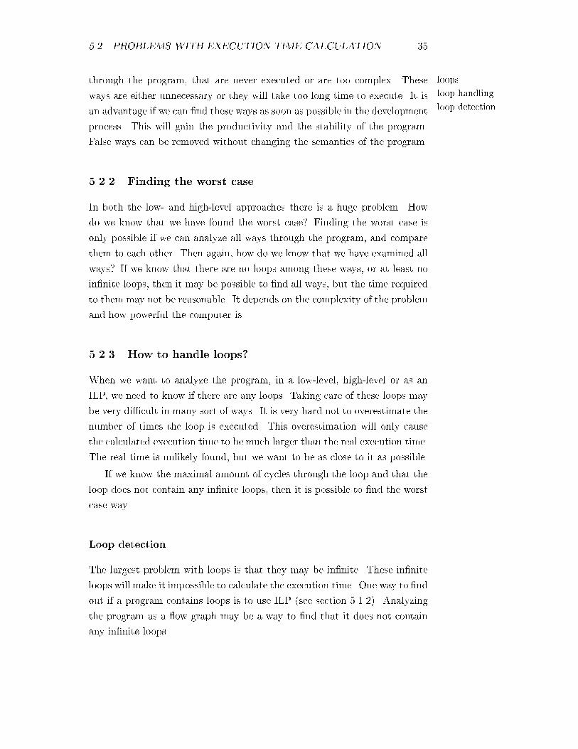
5.2. PROBLEMS WITH EXECUTION TIME CALCULATION 35
loops
loop handling
loop detection
through the program, that are never executed or are too complex. These
ways are either unnecessary or they will take too long time to execute. It is
an advantage if we can �nd these ways as soon as possible in the development
process. This will gain the productivity and the stability of the program.
False ways can be removed without changing the semantics of the program.
5.2.2 Finding the worst case
In both the low- and high-level approaches there is a huge problem. How
do we know that we have found the worst case? Finding the worst case is
only possible if we can analyze all ways through the program, and compare
them to each other. Then again, how do we know that we have examined all
ways? If we know that there are no loops among these ways, or at least no
in�nite loops, then it may be possible to �nd all ways, but the time required
to them may not be reasonable. It depends on the complexity of the problem
and how powerful the computer is.
5.2.3 How to handle loops?
When we want to analyze the program, in a low-level, high-level or as an
ILP, we need to know if there are any loops. Taking care of these loops may
be very di�cult in many sort of ways. It is very hard not to overestimate the
number of times the loop is executed. This overestimation will only cause
the calculated execution time to be much larger than the real execution time.
The real time is unlikely found, but we want to be as close to it as possible.
If we know the maximal amount of cycles through the loop and that the
loop does not contain any in�nite loops, then it is possible to �nd the worst
case way.
Loop detection
The largest problem with loops is that they may be in�nite. These in�nite
loops will make it impossible to calculate the execution time. One way to �nd
out if a program contains loops is to use ILP (see section 5.1.2). Analyzing
the program as a �ow graph may be a way to �nd that it does not contain
any in�nite loops.
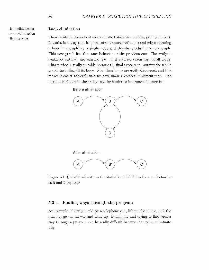
36 CHAPTER 5. EXECUTION TIME CALCULATION
loop elimination
state elimination
�nding ways
Loop elimination
There is also a theoretical method called state elimination, (see �gure 5.1).
It works in a way that it substitutes a number of nodes and edges (forming
a loop in a graph) to a single node and thereby producing a new graph.
This new graph has the same behavior as the previous one. The analysis
continues until we are satis�ed, i.e. until we have taken care of all loops.
This method is really suitable because the �nal expression contains the whole
graph, including all its loops. Now these loops are easily discovered and this
makes it easier to verify that we have made a correct implementation. The
method is simple in theory but can be harder to implement in practise.
A B C
D
Before elimination
A CB’
After elimination
Figure 5.1: State B' substitutes the states B and D. B' has the same behavior
as B and D together.
5.2.4 Finding ways through the program
An example of a way could be a telephone call, lift up the phone, dial the
number, get an answer and hang up. Examining and trying to �nd such a
way through a program can be really di�cult because it may be an in�nite
way.
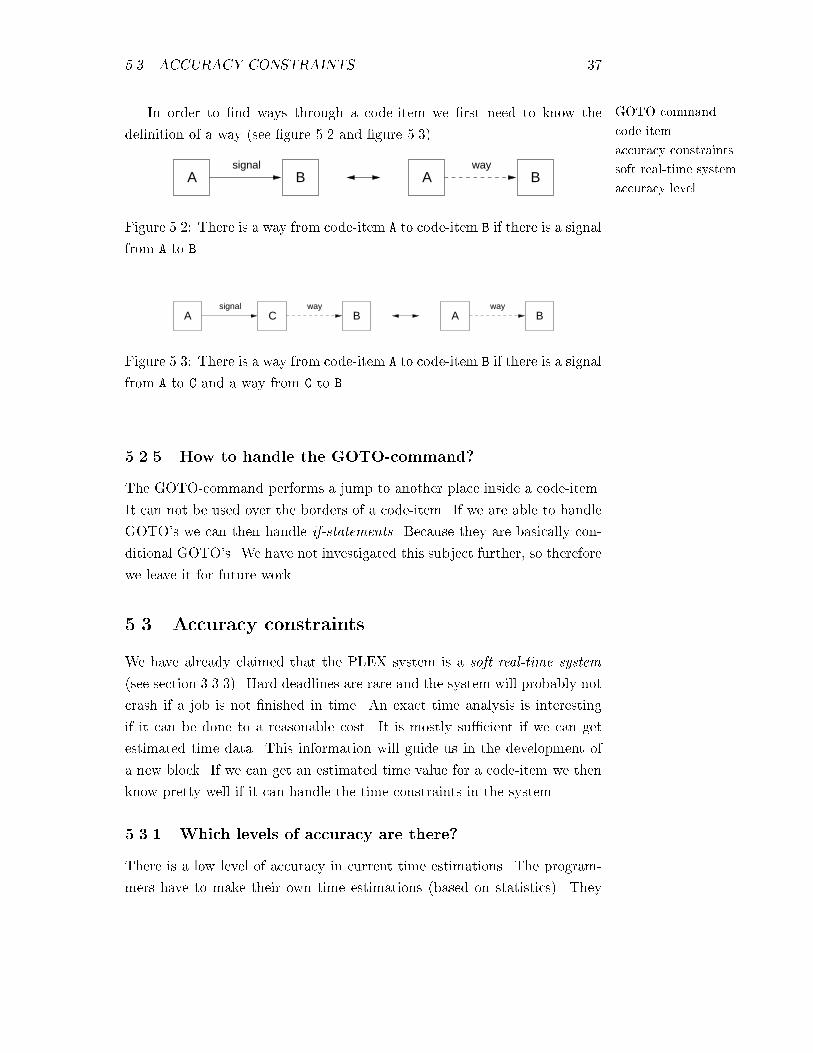
5.3. ACCURACY CONSTRAINTS 37
GOTO-command
code-item
accuracy constraints
soft real-time system
accuracy level
In order to �nd ways through a code-item we �rst need to know the
de�nition of a way (see �gure 5.2 and �gure 5.3).
A Bsignal
Away
B
Figure 5.2: There is a way from code-item A to code-item B if there is a signal
from A to B.
Asignal
C Bway
Away
B
Figure 5.3: There is a way from code-item A to code-item B if there is a signal
from A to C and a way from C to B.
5.2.5 How to handle the GOTO-command?
The GOTO-command performs a jump to another place inside a code-item.
It can not be used over the borders of a code-item. If we are able to handle
GOTO's we can then handle if-statements. Because they are basically con-
ditional GOTO's. We have not investigated this subject further, so therefore
we leave it for future work.
5.3 Accuracy constraints
We have already claimed that the PLEX system is a soft real-time system
(see section 3.3.3). Hard deadlines are rare and the system will probably not
crash if a job is not �nished in time. An exact time analysis is interesting
if it can be done to a reasonable cost. It is mostly su�cient if we can get
estimated time data. This information will guide us in the development of
a new block. If we can get an estimated time value for a code-item we then
know pretty well if it can handle the time constraints in the system.
5.3.1 Which levels of accuracy are there?
There is a low level of accuracy in current time estimations. The program-
mers have to make their own time estimations (based on statistics). They
38 CHAPTER 5. EXECUTION TIME CALCULATION
accuracy level are using tables with approximate execution times for PLEX- and assembler-
instructions. We can say it is based on guesses. These estimations then have
to cope with the actual time constraints. The programmers have to rely on
their experience of testing previous code-items.
Through testing the PLEX programmers have determined a maximum
amount of code rows for each code-item. This maximum can not be overrid-
den, because then it will not handle the actual time constraints. So we can
say it is some sort of a control. But the value have not been derived by any
exact execution time calculations.
Guidelines for PLEX programmers are that they should not write blocks
larger than a certain amount of code-rows. In most cases this is su�cient
to stay within execution time requirements. But there is no guarantee that
time requirements will not be violated.
5.3.2 Which level of accuracy do we choose?
It may be good to choose a level of accuracy that helps the programmer
through problematical sections. This help will not give the programmer any
proposals for di�erent solutions, but it will inform him or her that there are
risks that time constraints will be violated.
When showing the information regarding loops and GOTO's it may be
a good idea to view more information than actually needed. Producing very
detailed information may be easier than just giving the user information
about things that really are threats.
A conservative approach is to exclude the parts of the code that can be
guaranteed to be secure. If a possible threat is found, it is best to report it.
The programmer can easily weed out unimportant information.
It is hard to de�ne an adequate level of information. If too much is
shown, there are problems sorting out what is really important. This will
slow down the development process and make it harder to maintain. On the
other hand, if too little information is shown, some important warnings may
be missed, which may cause the product to be insecure and unstable. An
approach where the level of information is �exible would be suitable.
graphicalrepresentation
graphs
sub-graphs
GRETA
Graph Finder
Chapter 6
Graphical Representation
6.1 Introduction
Very often problems are presented as graphs to make them easier to under-
stand. A good picture or a good graph, can be very hard to outdo with
a text description. When programming, it can sometimes be hard survey
the structure because everything is written in code. Therefore drawing the
structure as a graph (or as many graphs) can sometimes be a solution.
6.1.1 Represent PLEX graphically
As already discussed in many other parts of this thesis, PLEX is a sys-
tem built upon signal communication. Signals are sent both internal (inside
blocks) and external (between blocks). If we want to construct an external
graph showing the communication between blocks, we can set the blocks as
nodes and the signals as edges (arcs). For the internal communication we
can draw sub-graphs. One sub-graph for each block. In these graphs, the
code-items are the nodes and the signals are the edges.
In our project GRETA, we have implemented a tool called Graph Finder
based on this theory. For more details see section 7.4.
6.1.2 Any existing graph standards for PLEX?
An interesting aspect, when talking about graph representation regarding to
PLEX, is standards. Are there any existing standards for showing PLEX
structures as graphs?
40 CHAPTER 6. GRAPHICAL REPRESENTATION
FDL
SDL
SDL-10
Petri nets
GRETA
Mealy machine
Moore machine
automatas
state machines
�ow chars
Finite Automata
Stack Automata
Push-Down Automata
Turing Machine
We know that some of the PLEX development is done in FDL (see section
6.4) and in a special version of SDL called SDL-10. Graphs created in SDL-
10 are later converted into pure PLEX code, but can not be transformed the
other way around (i.e. from PLEX code to SDL-10 graphs). SDL will be
further discussed in section 6.3.
Other graphical concepts used for designing parts of the AXE-system is
UML (see section 6.5) and MSC (see section 6.6).
We have further also found some connections between PLEX and a graph-
ical notation called Petri nets (more details in section 6.7). Maybe it is possi-
ble to map structures in PLEX to this notation. There are tools available for
creation and validation of Petri nets. If it is possible to map PLEX into this
notation it could also be reasonable to use these tools for analyzing PLEX.
What Petri net tools that could be interesting for PLEX analysis have not
been studied in detail during this thesis. This part is left for future work.
During the work with this thesis, no tools have been found that could
transform PLEX code to a graphical notation, except our own prototype tool
project GRETA. All analysis's in GRETA are done in logic programming
which may be su�cient. More details about the GRETA project can be
found in section 7.1.
6.2 Automata representation
It is often very suitable to represent data structures and formal methods as
automatas, i.e. state machines. They can be presented graphically as �ow
charts. The nodes are the states and the edges are the way to go from one
state to another.
State machines are usually ordered in a way depending on how powerful
they are. The simplest form is called Finite Automata (FA). These machines
can just read from an input string and write to an output string. They are
only able to use the latest visited state as a memory. The next variant
is Stack Automata or Push-Down Automata (PDA). They are a bit more
advanced than the FA's, because they can also use a stack memory to store
information. The most powerful state machine is the Turing Machine1 (TM).
The TM's use an in�nite tape memory instead of a stack.
1The Turing Machine was named by the famous British mathematician and computer
scientist Alan Turing (1912-1954).
6.3. SDL 41
SDL (Speci�cation andDescriptionLanguage)
CCITT
speci�cation language
implementationlanguage
When talking about Finite Automatas we commonly represent the prob-
lem either as a Moore machine or a Mealy machine. The di�erence between
them is where the action is done. Either in the nodes (the states) or in the
edges. In Moore machines the action is done in the states, even in the start
state. A Mealy machine does the action in the edges between the states.
6.3 SDL
SDL (Speci�cation and Description Language) is a standardized language
for specifying and describing systems. The system descriptions are built up
graphically and are therefore suitable for this chapter.
6.3.1 Introduction
The development of SDL started in 1972 by CCITT (International Telegraph
and Telephone Consultative Committee) and it was designed to specify and
describe the functional behavior of telecommunication systems. It is still
under development.
In early 1990's, object oriented features were included in the language.
Today SDL is widely used in a number of areas, telecommunication, aircraft,
train control and medical systems, real-time and interactive systems etc.
The use of a speci�cation language makes it possible to analyze and
simulate system solutions. Which in practice is much more di�cult when
using a textual programming language, due to the cost and the time delay.
A speci�cation language o�ers a set of well designed concepts for the use
of the language. One of these concepts can be to produce a solution to a
problem and to reason about a solution.
SDL covers di�erent levels of abstraction, from a broad overview to a
detailed design level. But the purpose with SDL, is not to be an implemen-
tation language. Though, automatic translation of SDL notation to a textual
notation is supported.
A basic theoretical model of an SDL system consist of a set of extended
�nite state machines that run in parallel. These machines are independent
of each other and communicate with discrete signals.
An SDL system consists of the following components:
� Structure-system, block, process and procedure hierarchy
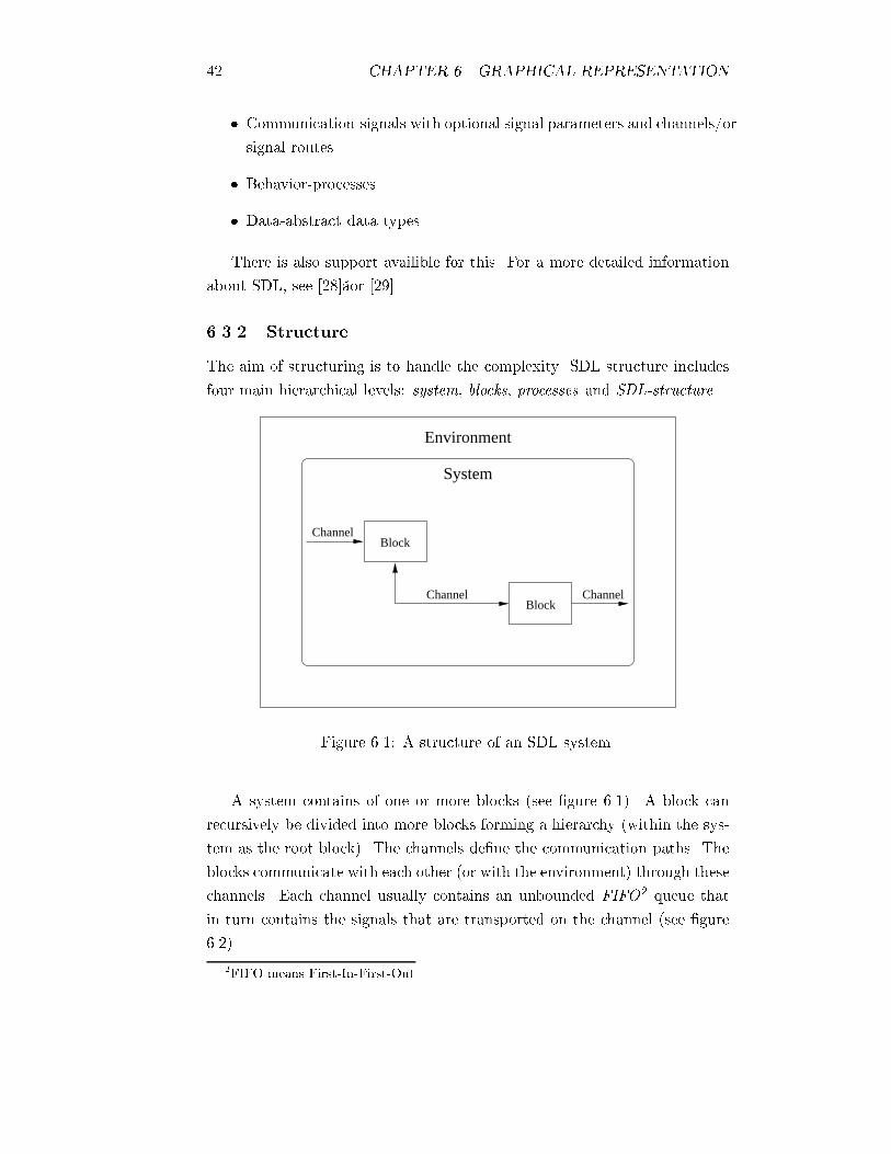
42 CHAPTER 6. GRAPHICAL REPRESENTATION
� Communication-signals with optional signal parameters and channels/or
signal routes
� Behavior-processes
� Data-abstract data types
There is also support availible for this. For a more detailed information
about SDL, see [28] or [29].
6.3.2 Structure
The aim of structuring is to handle the complexity. SDL structure includes
four main hierarchical levels: system, blocks, processes and SDL-structure.
Environment
System
Block
Block
Channel
Channel Channel
Figure 6.1: A structure of an SDL system.
A system contains of one or more blocks (see �gure 6.1). A block can
recursively be divided into more blocks forming a hierarchy (within the sys-
tem as the root block). The channels de�ne the communication paths. The
blocks communicate with each other (or with the environment) through these
channels. Each channel usually contains an unbounded FIFO2 queue that
in turn contains the signals that are transported on the channel (see �gure
6.2).
2FIFO means First-In-First-Out
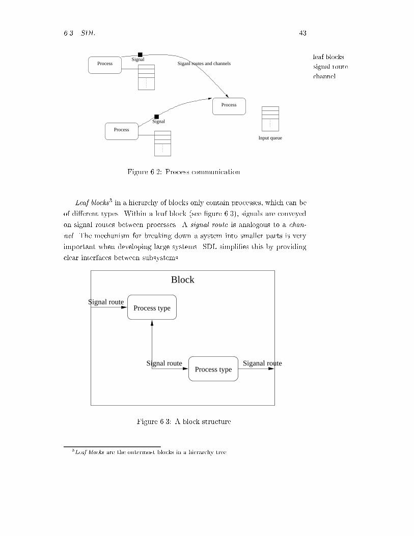
6.3. SDL 43
leaf blocks
signal route
channel
Process
Process
Process
Input queue
Siganl routes and channelsSignal
Signal
Figure 6.2: Process communication.
Leaf blocks3 in a hierarchy of blocks only contain processes, which can be
of di�erent types. Within a leaf block (see �gure 6.3), signals are conveyed
on signal routes between processes. A signal route is analogous to a chan-
nel. The mechanism for breaking down a system into smaller parts is very
important when developing large systems. SDL simpli�es this by providing
clear interfaces between subsystems.
Process typeSignal route
Process typeSiganal routeSignal route
Block
Figure 6.3: A block structure.
3Leaf blocks are the outermost blocks in a hierarchy tree
44 CHAPTER 6. GRAPHICAL REPRESENTATION
real-time systems
distributed systems
PId (Process Identi�er)
ADT (Abstract DataType)
6.3.3 Data sending
SDL does not use any global data. This approach requires that informa-
tion between processes, or between the processes and the environment, must
be sent with signals and optional signal parameters. Signals are sent asyn-
chronously and they can only be sent to one process instance at a time. This
part is one of the aspects where SDL di�ers from PLEX. An input queue is
associated with every process. This queue acts like a FIFO queue.
6.3.4 Timers
SDL de�nes time and timers in a clever and abstract manner. Time is
an important aspect in all real-time systems, but also in most distributed
systems. The timer is an object that is owned by a process. The timer
object is able to generate a timer signal and put this signal into the input
queue of the process.
6.3.5 Behavior
The dynamic behavior in an SDL system is described in the processes. The
system/block hierarchy is only a static description of the system structure.
Processes in SDL can be created at system start or at run time. More than
one instance of a process can exist. Each instance has a unique PId (Process
Identi�er) which makes it possible to send signals to individual instances
of a process. The concept of processes and process instances that work
autonomously and concurrently makes SDL a true real-time language.
6.3.6 Data
The data type concept in SDL is based on an ADT (Abstract Data Type)4.
This approach makes it easy to map an SDL data type to data types used
in other high-level languages.
6.3.7 SDL-10
Ericsson has a clearly stated goal to use more standard languages and prod-
ucts from the market. This has been one of the reasons to start working with
4An ADT (Abstract Data Type) is a data type with no speci�ed data structure. Instead,
it speci�es a set of values, operations (based on the values) and equations (that the
operations must ful�ll).
6.4. FDL 45
SDL-10
FDL (FunctionDescriptionLanguage)
SDL. For e�ciency reasons, to raise the abstraction level and for the reason
that SDL's process architecture is incompatible with the event triggered sig-
nal paradigm in PLEX, a number of changes have been done to SDL. These
changes have led to an Ericsson version of SDL, called SDL-10.
SDL-10 has been used in some projects. A theoretical evaluation from
code generation principles, indicates that the code size increase will be at
most 10%. This is also the upper limit indicated for the performance loss.
In SDL, signals do not appear in the top level. They are considered as
a lower level element. This aspect gives the wrong focus for AXE-10 design.
SDL as it without extension cannot be translated directly to PLEX. For
futher reading, see [9].
6.3.8 Advantages with SDL
SDL enables the user to produce a thorough system speci�cation and design.
We can say it own many advantages:
� It is an international standard
� It is formalized
� It is allowing simulation and complete code generation.
6.3.9 Disadvantages with SDL
SDL seems to be quite complex and it can take time to get familiar with
the language. Another disadvantage is that from SDL you cannot in general
produce a PLEX application system.
6.4 FDL
The FDL (Function Description Language) is a language for graphical rep-
resentation. It was developed by Ericsson in the 1980's because of the fact
that SDL did not work properly together with PLEX. FDL includes MSC's
(Message Sequence Charts) (see section 6.6), unit (block) program code �ow
diagrams and state transition diagrams.
46 CHAPTER 6. GRAPHICAL REPRESENTATION
UML (Uni�edModeling Language)
Booch
OMT
OOSE
object orientedlanguage
Grady Booch
Booch modelingmethod
Jim Rumbaugh
OMT (ObjectModeling Technique)
Rational Software
Ivar Jacobson
OOSE (ObjectOriented SoftwareEngineering)
6.5 UML
The UML (Uni�ed Modeling Language) is a language for specifying, visual-
izing and constructing the elements of software systems. It can also be used
for business modeling. UML is a uni�cation of the three most popular and
used modeling methods: Booch, OMT and OOSE.
6.5.1 Introduction
In the early 1990's object oriented programming languages had become popu-
lar. At this time software developers began to realize that a thorough model
of a software system is required to ensure architectural stability. There were a
number of modeling techniques available, but no one was a standard. So, the
need for a standard method came out from industry and not from academia.
In late 1994 Grady Booch5 and Jim Rumbaugh6 began to work on unifying
their modeling methods. This work began at Rational Software. During
1995, Ivar Jacobson7 joined Booch's and Rumbaugh's work. In 1997 the
�rst standard method was published, UML 1.0. It was later revised as version
1.1 in September the same year.
It was later revised as version 1.1 in September the same year. There is
a lots of information about UML on the Internet, one of those can be found
in [30]. For further reading see [10] and [11].
The three UML designers had a number of goals for the language:
� To be an expressive modeling language
� To enable the modeling of systems using object-oriented concepts
� To be independent of particular programming languages and develop-
ment processes
� To provide a formal basis for understanding the modeling language
� To derive advantages from object oriented paradigm and code reuse
� To support higher-level development concepts such as collaborations,
frameworks, patterns, and components.
5Grady Booch, famous for the Booch modeling method6Jim Rumbaugh, famous for the Object Modeling Technique (OMT)7Ivar Jacobson, founder of the Object Oriented Software Engineering modeling method
(OOSE)
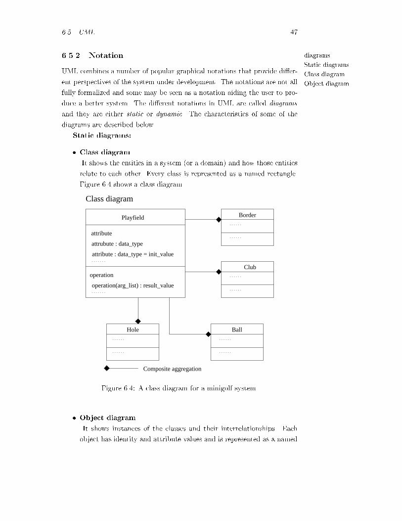
6.5. UML 47
diagrams
Static diagrams
Class diagram
Object diagram
6.5.2 Notation
UML combines a number of popular graphical notations that provide di�er-
ent perspectives of the system under development. The notations are not all
fully formalized and some may be seen as a notation aiding the user to pro-
duce a better system. The di�erent notations in UML are called diagrams
and they are either static or dynamic. The characteristics of some of the
diagrams are described below.
Static diagrams:
� Class diagram
It shows the entities in a system (or a domain) and how those entities
relate to each other. Every class is represented as a named rectangle.
Figure 6.4 shows a class diagram.
Playfield
attribute
attrubute : data_type
attribute : data_type = init_value
operation
operation(arg_list) : result_value
Class diagram
Border
BallHole
Club
Composite aggregation
Figure 6.4: A class diagram for a minigolf system.
� Object diagram
It shows instances of the classes and their interrelationships. Each
object has identity and attribute values and is represented as a named
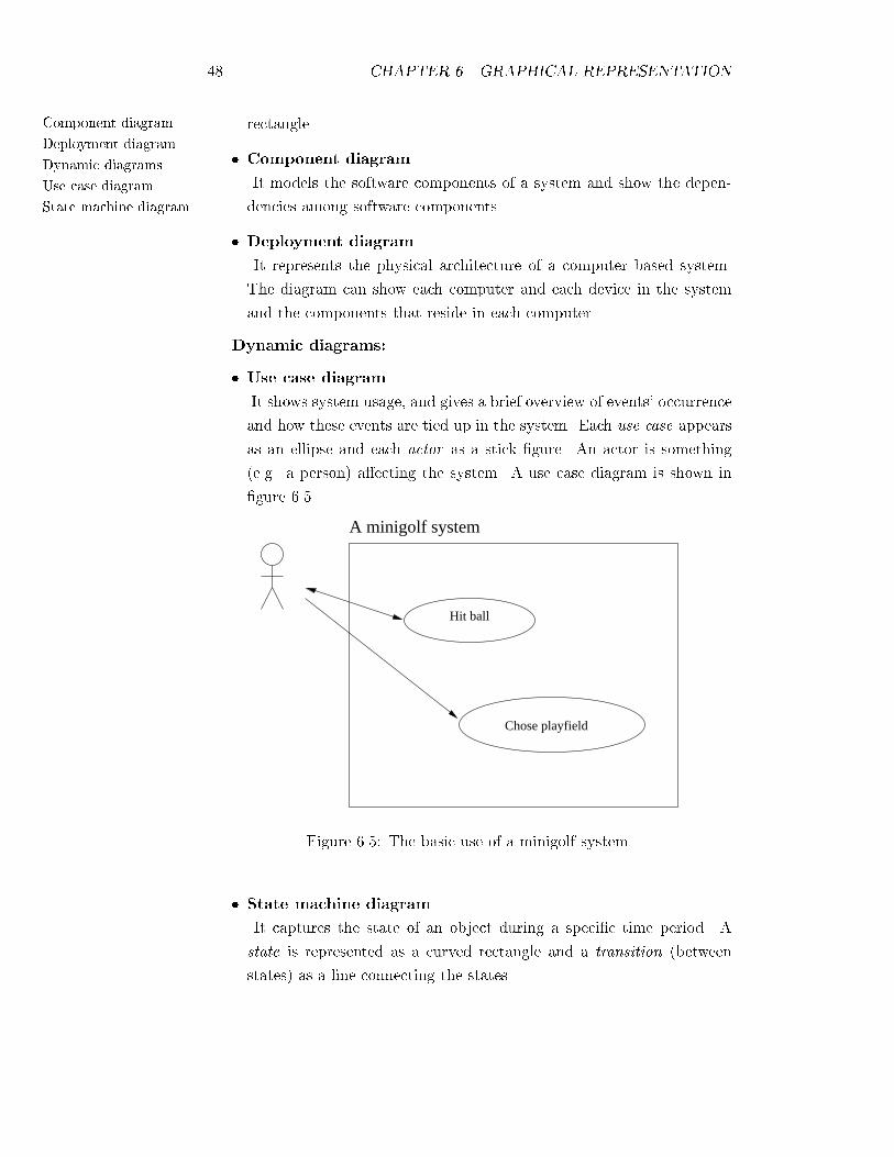
48 CHAPTER 6. GRAPHICAL REPRESENTATION
Component diagram
Deployment diagram
Dynamic diagrams
Use case diagram
State machine diagram
rectangle.
� Component diagram
It models the software components of a system and show the depen-
dencies among software components.
� Deployment diagram
It represents the physical architecture of a computer based system.
The diagram can show each computer and each device in the system
and the components that reside in each computer.
Dynamic diagrams:
� Use case diagram
It shows system usage, and gives a brief overview of events' occurrence
and how these events are tied up in the system. Each use case appears
as an ellipse and each actor as a stick �gure. An actor is something
(e.g. a person) a�ecting the system. A use case diagram is shown in
�gure 6.5.
Hit ball
A minigolf system
Chose playfield
Figure 6.5: The basic use of a minigolf system.
� State machine diagram
It captures the state of an object during a speci�c time period. A
state is represented as a curved rectangle and a transition (between
states) as a line connecting the states.
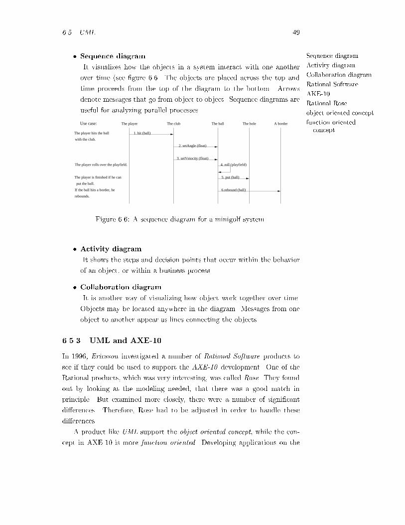
6.5. UML 49
Sequence diagram
Activity diagram
Collaboration diagram
Rational Software
AKE-10
Rational Rose
object oriented concept
function orientedconcept
� Sequence diagram
It visualizes how the objects in a system interact with one another
over time (see �gure 6.6. The objects are placed across the top and
time proceeds from the top of the diagram to the bottom. Arrows
denote messages that go from object to object. Sequence diagrams are
useful for analyzing parallel processes.
A border
6.rebound (ball)
The holeThe ball
4. roll (playfield)
3. setVeiocity (float)
2. setAngle (float)
1. hit (ball)
The clubThe playerUse case:
The player rolls over the playfield.
with the club.
The player hits the ball
5. put (ball)The player is finished if he can
put the ball.
If the ball hits a border, he
rebounds.
Figure 6.6: A sequence diagram for a minigolf system.
� Activity diagram
It shows the steps and decision points that occur within the behavior
of an object, or within a business process.
� Collaboration diagram
It is another way of visualizing how object work together over time.
Objects may be located anywhere in the diagram. Messages from one
object to another appear as lines connecting the objects.
6.5.3 UML and AXE-10
In 1996, Ericsson investigated a number of Rational Software products to
see if they could be used to support the AXE-10 development. One of the
Rational products, which was very interesting, was called Rose. They found
out by looking at the modeling needed, that there was a good match in
principle. But examined more closely, there were a number of signi�cant
di�erences. Therefore, Rose had to be adjusted in order to handle these
di�erences.
A product like UML support the object oriented concept, while the con-
cept in AXE-10 is more function oriented. Developing applications on the
50 CHAPTER 6. GRAPHICAL REPRESENTATION
MSC (MessageSequence Chart)
asynchronouscommunication
AXE-10 platform has been going on for 20 years now, so the development is
fundamentally working well. Therefore, the people that investigated a num-
ber of Rational products did not suggest any changes of existing processes
and methods in any fundamental way. UML is new and mostly used in small
or medium sized projects (for example in Germany). Therefore it has not
been used in projects at the size of a telecommunication system. An open
question is, how do we scale up UML?
6.5.4 Advantages with UML
Object oriented programming has been very popular for some years now.
The object oriented modeling techniques have also been developed to �t
object oriented systems. UML uses the object oriented paradigm in a clear
and useful way.
6.5.5 Disadvantages with UML
UML may not be suitable for systems that do not share the object oriented
paradigm. In these cases, changes have to be made in the development
process. It is also unknown how well UML can scale up to very large systems.
Compared with e.g. SDL, UML has a short track record and no strong
evidence for its advantages existing today. Therefore it can be a risk to use
UML.
6.6 MSC
The idea of a MSC (Message Sequence Chart) is to describe an example
part of the system behavior, not the complete behavior of a system. For a
more detailed speci�cation a collection of Message Sequence Charts can be
used. MSC contains descriptions of asynchronous communication between
instances. A basic MSC contains a description of the communication behav-
ior of a number of instances. An instance is an abstract entity of which one
can observe the interaction with other instances or with the environment.
An instance is denoted by a vertical axis. Figure 6.7 shows the commu-
nication behavior between instances i1, i2, i3 and i4. The time along each
axis runs from top to bottom. A communication between two instances is
represented by an arrow, which starts at the sending instance and ends at
the receiving instance.
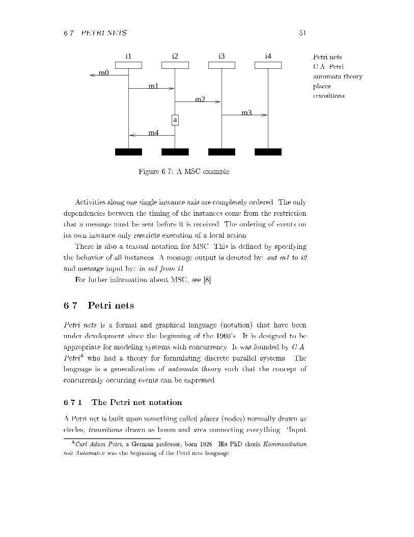
6.7. PETRI NETS 51
Petri nets
C.A. Petri
automata theory
places
transitions
m0
m1
m2
m3
m4
a
i1 i2 i3 i4
Figure 6.7: A MSC example.
Activities along one single instance axis are completely ordered. The only
dependencies between the timing of the instances come from the restriction
that a message must be sent before it is received. The ordering of events on
its own instance only restricts execution of a local action.
There is also a textual notation for MSC. This is de�ned by specifying
the behavior of all instances. A message output is denoted by: out m1 to i2
and message input by: in m1 from i1.
For futher information about MSC, see [8].
6.7 Petri nets
Petri nets is a formal and graphical language (notation) that have been
under development since the beginning of the 1960's. It is designed to be
appropriate for modeling systems with concurrency. It was founded by C.A.
Petri8 who had a theory for formulating discrete parallel systems. The
language is a generalization of automata theory such that the concept of
concurrently occurring events can be expressed.
6.7.1 The Petri net notation
A Petri net is built upon something called places (nodes) normally drawn as
circles, transitions drawn as boxes and arcs connecting everything. `Input
8Carl Adam Petri, a German professor, born 1926. His PhD thesis Kommunikation
mit Automaten was the beginning of the Petri nets language.
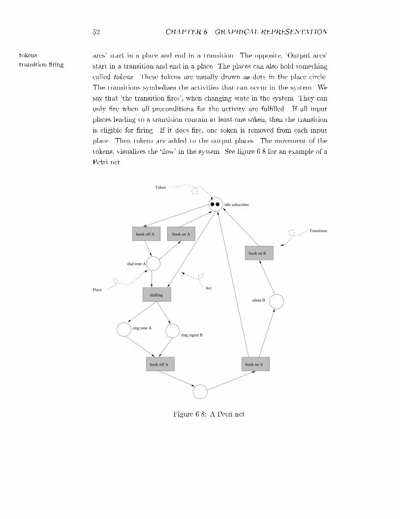
52 CHAPTER 6. GRAPHICAL REPRESENTATION
tokens
transition �ring
arcs' start in a place and end in a transition. The opposite, `Output arcs'
start in a transition and end in a place. The places can also hold something
called tokens. These tokens are usually drawn as dots in the place circle.
The transitions symbolizes the activities that can occur in the system. We
say that `the transition �res', when changing state in the system. They can
only �re when all preconditions for the activity are ful�lled. If all input
places leading to a transition contain at least one token, then the transition
is eligible for �ring. If it does �re, one token is removed from each input
place. Then tokens are added to the output places. The movement of the
tokens, visualizes the `�ow' in the system. See �gure 6.8 for an example of a
Petri net.
hook off A hook on A
dialling
ring tone A
ring signal B
hook off A hook on A
silent B
hook on B
idle subscriber
dial tone A
Transision
Token
Place Arc
Figure 6.8: A Petri net.
6.7. PETRI NETS 53
Black and white Petrinets
CPN (Coloured PetriNets)
Timed Petri nets
Stochastic Petri nets
�ring delays
6.7.2 `Black & White' and `Coloured' Petri nets
The simplest kind of Petri nets is the black and white nets. In these nets
the tokens can only represent one attribute. Therefore we can only have
one kind of arc leading from one place to another. In coloured nets we can
have di�erent kinds of tokens. Which means that the tokens are drawn in
di�erent colors representing di�erent functionality. In coloured nets we can
have more than one arc leading from one place to another, because the arcs
represent di�erent kinds of tokens. For example we can have a blue arc for
blue tokens and a red arc for red tokens, to be more concrete.
During the �ring of a transition in a coloured net, we have to get the
correct color of the token from the input. In the black and white nets we
just get an `arbitrary token' from the input, because all tokens there have the
same color (black). Because of the power to di�erentiate tokens by colors, the
notation of a coloured net is much more concise than a black and white net.
When modeling in coloured nets, we can also avoid a lot of the duplication,
which is typical in black and white nets.
6.7.3 Timed and Stochastic nets
Sometimes we want to simulate timed processes and delays to study per-
formance and dependability of the system. For example we know that the
actual code for a transition takes 10 ms. This can also be simulated with
Petri nets. The whole idea is based on setting delays either to the transi-
tions or the places. Having time delays on both transitions and places at the
same time is hard to model, therefore only one of the approaches is normally
chosen. Setting the delays on the transitions is the most common way to
go. We can say we set `�ring delays'. This delay speci�es the time that a
transition has to be enabled, before it can actually �re.
There are also di�erent ways of distributing the time delays. One ap-
proach is called Timed nets and it is based on a deterministic model where
the delay is �xed. Another approach is to distribute the delays randomly. It
is called Stochastic Petri nets. What model we choose, of course depends on
the practical problem.
54 CHAPTER 6. GRAPHICAL REPRESENTATION
asynchronouscommunication
CPN (Coloured PetriNets)
CPN editor
CPN simulator
SDL
6.7.4 Advantages with Petri nets
Then let us summarize the advantages with Petri nets. First of all we see
that the notation and the semantics is very well founded in theory. This
leads to powerful possibilities to analyze the system.
Another important bene�t is that Petri nets allow asynchronous com-
munication. They are neither centered around the process concept. This
makes Petri nets suitable for systems like AXE and other dealing with tele-
communication.
6.7.5 Disadvantages with Petri nets
The most obvious drawback with Petri nets is that they are mainly used
in research so far. In theory they are well founded, but there is no actual
standard right now. Many di�erent variants of Petri nets are used. There
are some tools available for Petri nets (see section 6.7.6) and some of them
have been used in a few industrial projects, but despite this Petri nets are
not so well known yet.
6.7.6 Tools for Petri nets
There are a number of tools available for editing, validating and simulating
CPN (Coloured Petri Nets). Some of them have also been used in some
industrial projects.
The CPN editor allows us to work with large diagrams (hierarchical
CPN's) which have 50-100 pages, each with 5-25 nodes and 10-50 arcs. It
allow us to construct and modify them graphically on the computer screen
using a mouse. There is also built-in support for syntax checking. The tool
is available for Macintosh and UNIX (X-Windows) machines.
The CPN simulator is another tool which is closely integrated with the
CPN editor. In the simulator it is possible to simulate a �ow in a CPN. First
you can create a CPN in the editor and then simulate it in the simulator.
Such a simulation can perhaps be helpful when debugging.
More information about the tools for CPN's can be found in [21].
6.7.7 Petri nets in PLEX environment
It has already been shown that designs made in SDL can be translated into
Petri nets. Graphical objects in the SDL-notation can be converted to similar
6.7. PETRI NETS 55
SDL-10objects in the Petri net environment. There are studies done in this subject,
for example in [5].
We also know that it is possible to generate PLEX code from programs
designed in SDL-10 (see section 6.3.7). Therefore it may be possible to go
from Petri nets to SDL and then to PLEX, at least when implementing parts
of a system.
But. . . if we study SLD-10 and PLEX, we see that SDL-10 is not able
to encompass the whole PLEX language. It can just represent a subset of
it. An interesting question appear. Can Petri nets represent a larger subset
of PLEX, or maybe cover the whole PLEX language? This question is not
answered properly in this thesis, but some pieces of the puzzle have been
found.
Theoretically, the structure of Petri nets seems to be closer to the PLEX
structure than SDL, because of the concurrent concept. SDL is also more
process-oriented, which is wrong approach when designing concepts like the
one in PLEX. But as far as we know now, there are no Petri net tools avail-
able, that are custom-made for PLEX. So we can not show this in practice.
GRETA
Facts Finder
facts-�le
Structure Finder
Graph Finder
Chapter 7
Prototypes
7.1 GRETA
During this thesis we have managed to create a prototype for a tool concept
we have called GRETA, which is an abbreviation for GRaphical Extractor
and Time Analyzer. This concept is supposed to be used during the PLEX
coding phase. Actually today GRETA is a compilation of three smaller tools
(see �gure 7.1). Two of them have been implemented and one is left for future
work.
� Tool one, Facts Finder , is the unimplemented tool which is left for
future work. Its main purpose is to pick out signaling facts from the
PLEX environment (various source-�les). Both signal information and
time data is supposed to be written in a facts-�le. This �le is now
generated manually.
� Tool two is Structure Finder , which has been implemented. This
tool is using the facts-�le created by the Facts Finder. By analyzing
the facts, this tool derives the signaling connections in the system. The
structure is then written to an intermediate format read by a third tool.
� Tool three, Graph Finder , which also has been implemented, is using
the intermediate format �le created by the Structure Finder. Graph
Finder is able to create graphs and sub-graphs of the PLEX structure.
The graphs can also be weighted with time data.

7.1. GRETA 57
Data file for storingof coordinates
Intermediate formatwith description ofblocks, signals andtime data
write
read
read
write
read
PLEXfile
PLEXfile
write read read
Parts we have not implemented
created manually
Structure Finder Facts Finder
Graph Finder
Facts-file
This file is now
The structure of GRETA
Figure 7.1: A �ow chart over the GRETA structure.
58 CHAPTER 7. PROTOTYPES
Facts Finder
PLEX-compiler
signal survey
Structure Finder
Prolog
facts-�le
ILP
PLEX-compiler
7.2 Facts Finder
Facts Finder is a tool that collects facts regarding signals and blocks. Typical
facts are which signals there are and their execution times and also what
blocks they are connected to. These facts will be used in the Structure
Finder tool.
Here we will theoretically describe the Facts Finder tool. This tool is
rather complex and advanced, therefore there have not been enough time to
investigate and implement this further, so we have left it for future work.
7.2.1 Storing the facts
First of all we have to decide what kind of facts we need. Information for
blocks, signals and code-items is needed.
We have found out that it is possible to receive these logical facts by
scanning various source �les and by output from an extended variant of the
code generator (in the PLEX-compiler). Signals are found in the PLEX
source code and in the signal survey1. Code-items are found in the PLEX
source code.
We also want to know when each signal is sent from a code-item. Today
the code generator is not able to bring us this information. Finding the
execution time is a problem that has to be solved. (See chapter 5).
The Structure Finder tool is implemented in a declarative language called
Prolog . Therefore we have chosen to write our facts-�le in Prolog syntax.
The Facts Finder is not yet implemented and therefore we have created the
facts-�le manually.
These facts and the facts-�le are described further in Intermediate format
in appendix I.
7.2.2 Execution time calculation
While the Facts Finder is unimplemented, we have to write arbitrary time
values in the facts-�le. There are no other tools available either, that can
help us to get correct execution time information of the signals.
We have to decide where we want the Facts Finder to get the information.
Either via ILP (see section 5.1.2) or from an extended version of the PLEX-
compiler.
1The signal survey is a �le that describes all signals sent from a certain block
7.3. STRUCTURE FINDER 59
Structure Finder
Prolog
pseudo-code
7.2.3 Implementation
We need to decide what programming language we should use to write this
Facts Finder. It would be suitable to choose a language that supports and
makes it easy to scan various source �les and extract information from them.
7.3 Structure Finder
Until now, there has not been any tool that can scan the PLEX-code and
�nd the �ow in the structure. When �nding the �ow, i.e. get the signaling
connections between di�erent blocks, logic programming comes at hand. In
this section we are going to describe a prototype tool we developed that is
able to perform such a task.
7.3.1 Programming in Prolog
Finding the signaling structure in PLEX is a problem that can be converted
to logical facts and rules. These facts consist of information about the signals
and the blocks in PLEX. The rules are based on these facts and they describe
our problem. With a programming language like Prolog we are able to deduce
the connections through the rules (and the facts) by giving the right queries.
7.3.2 Pseudo-code for our prototype in Prolog
When the main function (�gure 7.2) in Structure Finder is started, it �rst
opens a �le for writing. Opening a �le is a built-in function in Prolog. This
�le will contain all blocks and all signals between these blocks.
Next thing to do is to print the information about blocks and signals to
the �le. It is done in two steps:
� The �rst step calls the function show-information-for-all-blocks (see
�gure 7.3)
� Next step calls the function show-all-connections-between-blocks (see
�gure 7.4).
In order to print the information regarding all blocks, we �rst need to
�nd them. This is done by calling the function �nd-all-blocks. This function
just returns a list of the block names.
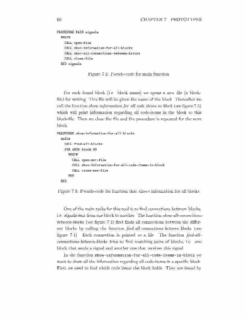
60 CHAPTER 7. PROTOTYPES
PROCEDURE MAIN signals
BEGIN
CALL open-file
CALL show-information-for-all-blocks
CALL show-all-connections-between-blocks
CALL close-file
END signals
Figure 7.2: Pseudo-code for main function.
For each found block (i.e. block name) we opens a new �le (a block-
�le) for writing. This �le will be given the name of the block. Thereafter we
call the function show-information-for-all-code-items-in-block (see �gure 7.5)
which will print information regarding all code-items in the block to this
block-�le. Then we close the �le and the procedure is repeated for the next
block.
PROCEDURE show-information-for-all-blocks
BEGIN
CALL find-all-blocks
FOR EACH block DO
BEGIN
CALL open-new-file
CALL show-information-for-all-code-items-in-block
CALL close-new-file
END
END
Figure 7.3: Pseudo-code for function that shows information for all blocks.
One of the main tasks for this tool is to �nd connections between blocks,
i.e. signals sent from one block to another. The function show-all-connections-
between-blocks (see �gure 7.4) �rst �nds all connections between the di�er-
ent blocks by calling the function �nd-all-connections-between-blocks (see
�gure 7.4). Each connection is printed to a �le. The function �nd-all-
connections-between-blocks tries to �nd matching pairs of blocks, i.e. one
block that sends a signal and another one that receives this signal.
In the function show-information-for-all-code-items-in-block we
want to show all the information regarding all code-items in a speci�c block.
First we need to �nd which code-items the block holds. They are found by
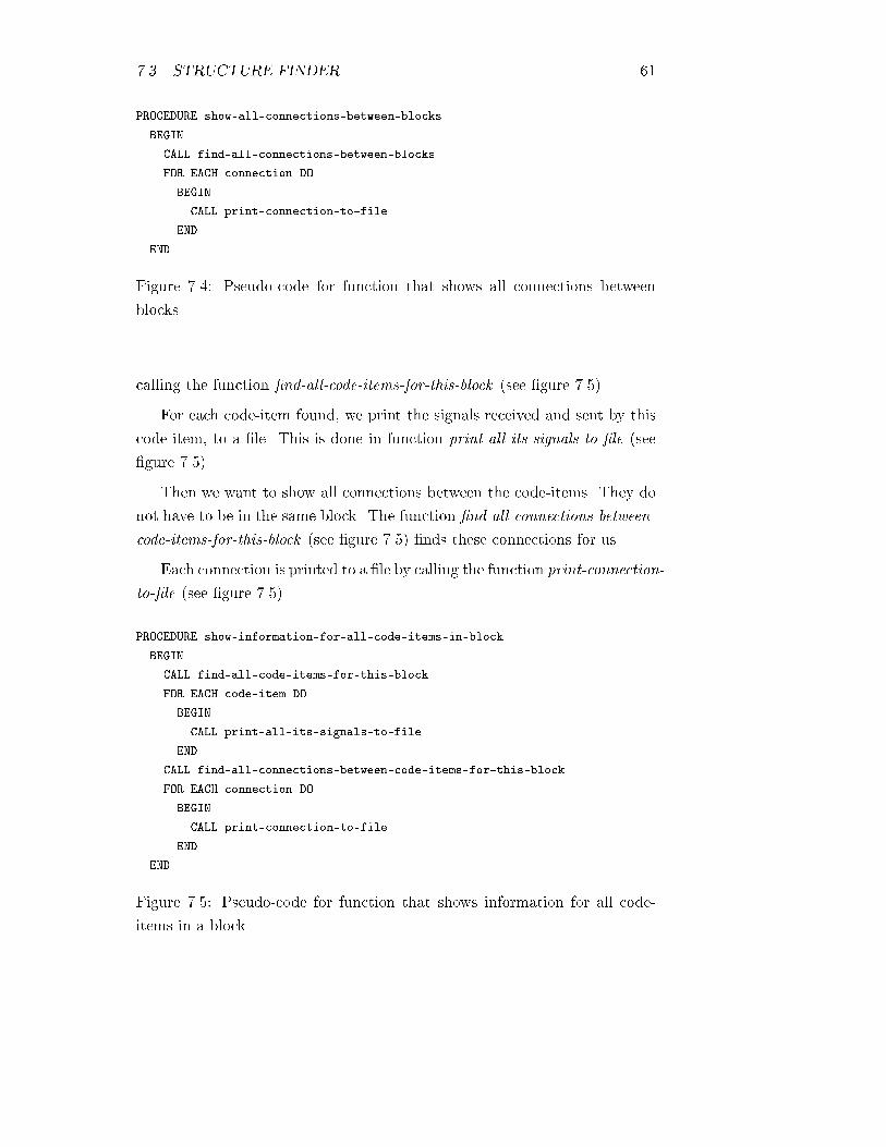
7.3. STRUCTURE FINDER 61
PROCEDURE show-all-connections-between-blocks
BEGIN
CALL find-all-connections-between-blocks
FOR EACH connection DO
BEGIN
CALL print-connection-to-file
END
END
Figure 7.4: Pseudo-code for function that shows all connections between
blocks.
calling the function �nd-all-code-items-for-this-block (see �gure 7.5).
For each code-item found, we print the signals received and sent by this
code-item, to a �le. This is done in function print-all-its-signals-to-�le (see
�gure 7.5).
Then we want to show all connections between the code-items. They do
not have to be in the same block. The function �nd-all-connections-between-
code-items-for-this-block (see �gure 7.5) �nds these connections for us.
Each connection is printed to a �le by calling the function print-connection-
to-�le (see �gure 7.5).
PROCEDURE show-information-for-all-code-items-in-block
BEGIN
CALL find-all-code-items-for-this-block
FOR EACH code-item DO
BEGIN
CALL print-all-its-signals-to-file
END
CALL find-all-connections-between-code-items-for-this-block
FOR EACH connection DO
BEGIN
CALL print-connection-to-file
END
END
Figure 7.5: Pseudo-code for function that shows information for all code-
items in a block.
62 CHAPTER 7. PROTOTYPES
execution timecalculation
Graph Finder
Graph Finder
graphs
Graph Finder
SDL-10
7.3.3 Execution time for a job
If we think of a scenario where we have all time information we need, how
would we calculate the execution time for a job?
We know (by a time value) when each signal is sent and therefore we
can sum these time values for a job to get the total execution time. First
we need to know what a job is. A job is an execution starting at a bu�ered
signal entry and ending at an EXIT-statement. All bu�ered signals can be
seen as jobs and the direct signals as parts of them.
To calculate the worst case possible job time, we consider a job as all
possible job paths starting with a particular bu�ered signal. In practice this
is not as easy as it seems. There may be loops in a path which have to
be handled. This is a di�cult problem and we discuss it theoretically in
section 5.2.3.
The execution time calculation for a job may be done either in the Struc-
ture Finder (see section 7.3) or in the Graph Finder (see section 7.4). In
Prolog, we can use the same search functionality that we used when search-
ing for the signaling structure. In Java it is a bit more complicated, because
we have to design our own search functionality (with while-statements, etc.).
Therefore, calculating the execution time for jobs in Structure Finder seems
to be a feasible approach.
7.4 Graph Finder
In this section we are going to describe a graph drawing tool called Graph
Finder, we developed to survey the PLEX structure.
7.4.1 Introduction
When analyzing PLEX, we noticed that it would be a good idea to have a
tool for transforming the PLEX code into a graphical notation. Basically
because it was very hard to survey all signal connections between the blocks
and inside a block. We knew that it existed graphical concepts like SDL-10
for generating `from graph to code', but we did not �nd anything that did
the opposite, `from code to graph'. So, we wanted to create a general tool
that could handle this kind of `reverse engineering'.
As already discussed in other sections, there is just a subset of the PLEX
functionality that can be expressed in SDL-10. The rest has to be done in
7.4. GRAPH FINDER 63
execution timecalculation
signal paradigm
PLEX from the beginning. So there are no tools for showing these `pure
PLEX sections' graphically.
We wanted to develop a general tool that could take any kind of PLEX
code, analyze it and then make a graphical representation of the structure.
Graphs often make it easier to �nd in�nite loops and `dead code' that never
runs. If the graph is weighted with execution time calculations , it can also
help us to �nd places that may be optimized later on.
An important thing about showing the PLEX structure as a graph, is
that we can get a survey of the whole system. Today, an AXE system has
about 350 internal working blocks. A block is approximately 20.000 lines
of code. One person is responsible for each block. Therefore many PLEX
programmers are just familiar with smaller parts of the code. The rest is just
like an unexplored land mass. With a graph tool that easily can show the
connections in the system in a nice and functional way, without being too
speci�c, the PLEX programmers can also understand the most important
structure in this unexplored land mass. They can see what the neighbor
blocks are doing and even analyze them critically. After using such a tool,
maybe it turns out that some PLEX programmers can see unoptimized parts
at the neighbors, that the neighbors have not discovered by themselves.
7.4.2 Abstraction level, views and layout
A question we have to ask before making a graph is, what do we want to
show? A graph can easily be very messy if it is too detailed. It can also
be very unnecessary if it lacks a lot of important information. Therefore we
have to be careful when deciding what to show and what to hide.
In a PLEX system everything is based on a signal paradigm. So it comes
quite natural that the signals is a very important part if we are going to
make a graph of the PLEX structure. In a global perspective it is also quite
important to show how the blocks are related to each other. Therefore we
can set the blocks as nodes and the signals as directed edges when showing
a graph of the global PLEX structure.
If we also show the names of the blocks and the signals we have a quite
good graph showing the �ow between the blocks. Then we can also weight
the graph with time values on all signals (edges). The value can be the
estimated time it takes before entering the goal block. Suddenly we have an
even more informative graph. We can now see all connections between the
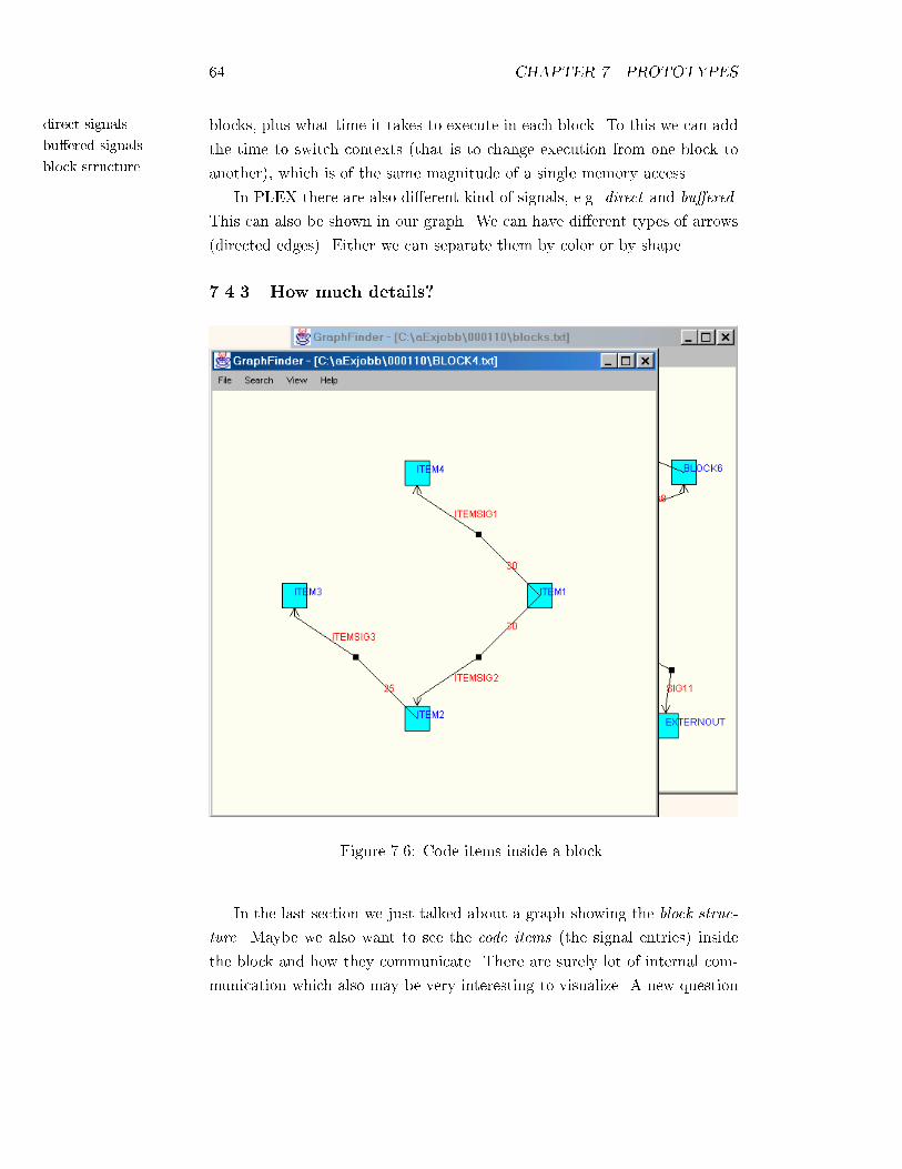
64 CHAPTER 7. PROTOTYPES
direct signals
bu�ered signals
block structure
blocks, plus what time it takes to execute in each block. To this we can add
the time to switch contexts (that is to change execution from one block to
another), which is of the same magnitude of a single memory access.
In PLEX there are also di�erent kind of signals, e.g. direct and bu�ered.
This can also be shown in our graph. We can have di�erent types of arrows
(directed edges). Either we can separate them by color or by shape.
7.4.3 How much details?
Figure 7.6: Code-items inside a block.
In the last section we just talked about a graph showing the block struc-
ture. Maybe we also want to see the code items (the signal entries) inside
the block and how they communicate. There are surely lot of internal com-
munication which also may be very interesting to visualize. A new question
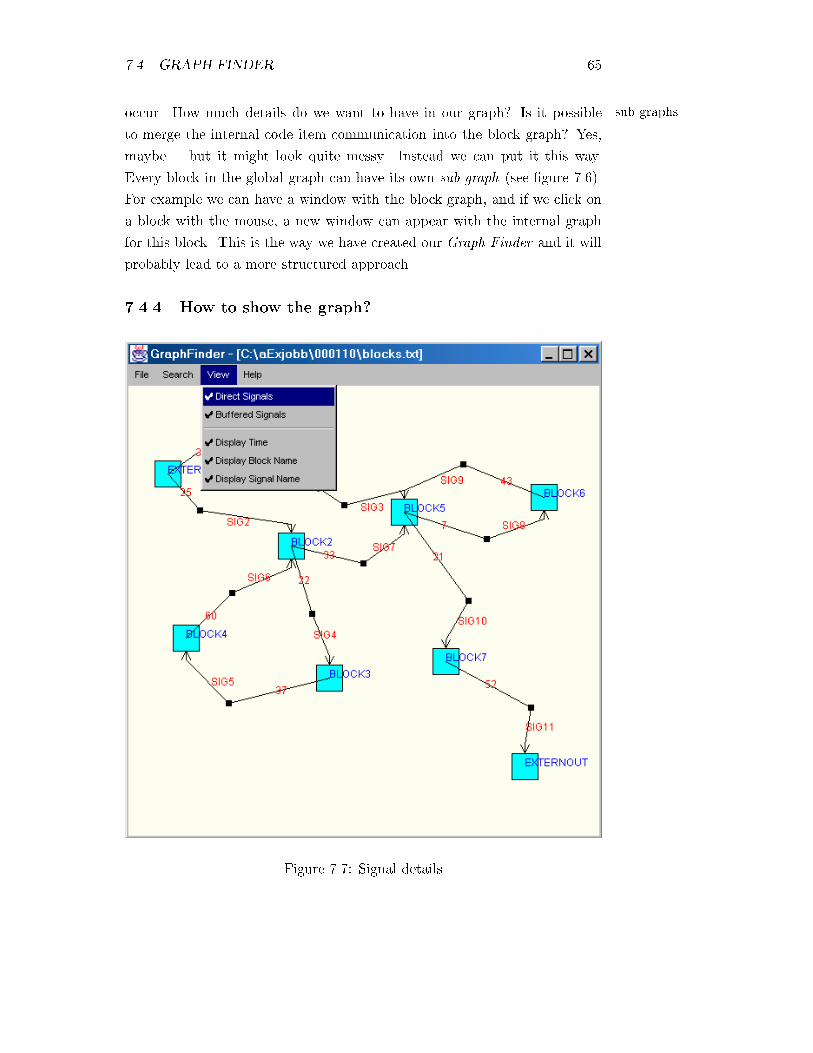
7.4. GRAPH FINDER 65
sub-graphsoccur. How much details do we want to have in our graph? Is it possible
to merge the internal code item communication into the block graph? Yes,
maybe... but it might look quite messy. Instead we can put it this way.
Every block in the global graph can have its own sub-graph (see �gure 7.6).
For example we can have a window with the block graph, and if we click on
a block with the mouse, a new window can appear with the internal graph
for this block. This is the way we have created our Graph Finder and it will
probably lead to a more structured approach.
7.4.4 How to show the graph?
Figure 7.7: Signal details
66 CHAPTER 7. PROTOTYPES
Java
crossing lines
optimization
There are many ways to show the graph on the screen. We have chosen
to implement the Graph Finder in the language Java. It is an application
with a window showing the graph. Above the actual graph there is a menu
bar with several functions and features. For example there is a view menu
with options to toggle what should be shown and what should not, in the
graph view (see �gure 7.7). If you are just interested to see the names of the
signals, you can simply hide the time values if you think they make the view
too detailed.
When clicking on a block, a new window will appear with a graph showing
the internal structure of this block, i.e. all code items and their signals.
7.4.5 Avoiding `crossing lines'
A big problem with graphs is to avoid crossing lines. Which means that
it is hard to avoid that two or more edges between nodes are crossing each
other. If we do not take care of this problem it can easily make the view look
unstructured and hard to understand. This problem can, as a suggestion,
be �xed in two ways. Either by structuring the nodes and edges manually
or automatically.
In Graph Finder we have chosen the �rst approach. You have the possi-
bility to manually drag and drop the nodes as you want by using the mouse.
It is fairly easy for a human being to see on the screen which lines that are
crossed and which are not.
The second approach is to make the computer �nd out how to avoid the
crossing lines. This is done, probably by using some sort of an algorithm. If
the graphs are wide, these algorithms can be quite complicated and heavy
to compute. We have not either investigated this subject further.
7.4.6 Input to our graph
In computers we store our data textual or binary as streams of characters.
We can not store a picture or a graph without being �rst translated into
a textual or binary format. Therefore it can be quite important to `think
twice' when designing the �le format for a graph. Here is a list of things to
take care of:
� Optimization
Do not include more than necessary
7.4. GRAPH FINDER 67
scalability
scalability
� Structure
Information should be listed in a structured order
� Scalability
It should be possible to expand or shrink the data amount.
In our case, the input �le for this Graph Finder tool, is created by the
Structure Finder. We have tried to follow these rules, listed above, when
creating the format.
7.4.7 A scalable tool
If we are going to develop a tool, it is very good if it is scalable. This means
that it is possible to add or remove functionality from the tool without
destroying the whole structure. As the time goes by, a system may change.
New data are included, old-fashioned data are removed. A well designed tool
can easily be expanded to handle these `new features' if it has to. Therefore,
�le formats should be �exible for changes, the window should be adapted to
draw more details, etc.
PLEX
FORTRAN
execution timecalculation
Chapter 8
Summary
8.1 Problem de�nitions
In this �rst section of the summary, we are going to give you the most
important questions at issue, regarding to the work of this thesis.
8.1.1 Language and system analysis
As a language PLEX can be pretty hard to describe and classify because
of its unique structure. Is it possible to map the structure of PLEX to any
other programming language?
The syntax in PLEX is in some places very close to old code written in
a language like FORTRAN. It is built on the standards that were common
in the 1970's and generally spoken, it has not been modernized too much
over the years. Is PLEX a language well suited for the younger generation
of programmers?
A telecommunication system has about 350 internal working blocks. A
block is approximately 20.000 lines of code. One person is responsible for
each block. Therefore it might be di�cult for a programmer working with
block A to get a good knowledge of what the neighbor programmers are
doing in block B or C. Is it possible to make the structure easier to survey?
8.1.2 Execution time calculation
The most important problem to take care of if we are going to do execution
time calculations in PLEX is to get the time of the signals. If it is possible
to receive signal time data it is possible to analyze the system properly
8.2. SUMMARY OF OUR WORK 69
graphicalrepresentation
event triggered
real-time systems
APZ
AI (Arti�cialIntelligence)
agent
Prolog
HL-PLEX
C language
Pascal
Petri nets
according to time. How can we receive execution time information from
signals in PLEX. . . and how do we calculate the time of a job?
8.1.3 Graphical representation
When thinking of graphical representation of PLEX code it is a problem that
the system is very large and complex. How are we going to present such a
huge system in a nice and functional way graphically?
8.2 Summary of our work
8.2.1 Language and system analysis
Mapping PLEX to other languages?
We have found that PLEX is a very unique language with an original struc-
ture. It is event triggered and based on a soft real-time system. PLEX is
also closely connected to the hardware APZ. All these aspects makes AXE
a quite fast system.
We have also seen that it might be possible to translate the PLEX block
structure to arti�cial intelligent agents. Maybe based on clauses written in
Prolog, which seems to be a good language to analyze structures in PLEX.
We have also come in contact with a language called HL-PLEX. It is
a modern and di�erent form of PLEX which seems to be more close to
languages like C and Pascal in its structure.
We have further also found some connections between PLEX and a graph-
ical notation called Petri nets. Maybe it is possible to map structures in
PLEX to this notation. There are tools available for creation and validation
of Petri nets. If it is possible to map PLEX into this notation it could also
be reasonable to use these tools for analyzing PLEX. Which Petri net tools
that could be interesting for PLEX analysis have not been studied in detail
during this thesis. This part is left for future work.
PLEX and the younger generation?
We know that PLEX has been extended several times since the start. But
despite this, the syntax feels quite old-fashioned if we study it today (January
2000). This is maybe comfortable for older programmers who are used to
this environment. But all we working with this thesis are educated in the
70 CHAPTER 8. SUMMARY
SDL-10
SDL
GRETA
high-level analysis
low-level analysis
ILP
graphs
sub-graphs
1990's and are therefore more familiar with modern forms of syntax. This is
probably something to think of when recruiting new employees to Ericsson
in the future.
How to survey the structure?
There are graphical tools available for designing AXE structures in a notation
called SDL-10. Graphs created in SDL can then be transformed into pure
PLEX code but not the other way around.
So during this thesis no tools have been found that could transform PLEX
code to a graphical notation. As a result of this we have designed a tool
concept called GRETA, running on prototype basis right now. All analyzing
in GRETA are done in logic programming which may be su�cient. More
details about the GRETA project can be found in section 7.1.
8.2.2 Execution time calculation
The execution time information of a signal can be received by analyzing
the code behind it. This can be done either on high-level basis (the PLEX
code) or on low-level (the assembler code). High-level analyzing can be done
by using algorithms like ILP , etc. Low-level analyzing can be done in the
compiler by comparing and calculating clock ticks on assembler instructions.
See chapter 5 for more details.
If we have all this execution time information about the signals in PLEX,
it is also possible to calculate the execution time of jobs. This is done by
summarizing the time information from each signal included in the job. If we
can do this, we have the possibility to �nd paths in the signaling structure,
that perhaps are slow or unnecessary. Out of this we can get hints on where
optimizations can be done. Maybe it will lead to a system, which is more
e�ective than today.
8.2.3 Graphical representation
As a result of studying PLEX and graphical notation we have seen that it is
possible to represent the PLEX structure as graphs in a nice and functional
way. Early in this process we thought it would be best to split the PLEX
structure into sub-graphs. One sub-graph for each block and a global graph
8.3. CONCLUSIONS 71
modularity
garbage collection
showing how the blocks communicate. In PLEX, signals are already divided
in di�erent blocks so this sub-graph classi�cation is quite natural.
8.3 Conclusions
We are now going to come up with some conclusions regarding to our studies
of the PLEX language.
8.3.1 What makes PLEX a good language?
There are some things that de�nitely makes PLEX a good language. First
of all the modularity. The structure with the blocks makes the whole system
very modular. This also leads to a very safe system. PLEX is also very secure
because it has been developed during a very long time, at least two decades,
almost three. The system is also very fast because of the close connection to
the hardware and the custom-made event triggered soft real-time system.
The memory management is also controlled by the programmer, there
is no automatic memory handling (a.k.a. garbage collection). This kind of
manual handling can be very good sometimes, because automatic methods
can be very complex and cause much overhead, which in turn can lead to
crashes. This overhead problem is very common today, in modern systems
using automatic handling. But manual memory management can also be a
drawback (see section 8.3.2).
The best thing with PLEX is though that it is still working. It have
been used since the 1970's and people are still using it in AXE-systems all
over the world. Actually, we can not say today if this depends on that there
have been no other alternatives or if PLEX has been the ultimate language
on the market. Despite this, the long life of PLEX is probably the best
acknowledgment the language can get.
8.3.2 What makes PLEX a less attractive language?
Tele-communication systems grow fast and are very complex. The code is
also quite hard to learn because of its special syntax. We also think it is a
drawback that both the syntax and the semantics seem to be quite obsolete.
It can be hard to introduce younger programmers into this. Because they are
not grown up with FORTRAN syntax which was popular in the seventies.
What will happen when all experienced PLEX programmers retire?
72 CHAPTER 8. SUMMARY
Prolog
Java
real-time system
APZ
GRETA
In PLEX there are also many compiling phases before we �nally receive
the binary code for the hardware. If we study this compiling structure it
seems to be quite complex and bit messy. Much of this mess depend on
compatibility constraints with older versions and connections with other lan-
guages etc. But it must be some way to make the compilation simpler and
less complex.
In section 8.3.1 we said it can be a good thing that the memory manage-
ment is controlled manually, by the programmer. This can also be a huge
drawback. Everything is based on the fact that the programmers do not
make any mistakes when writing the instructions for the memory handling.
In modern languages (e.g. Prolog and Java) we often see that the memory
management is built in the language and handled automatically. In PLEX
there is no automatic memory handling. Everything is controlled by the
programmers.
When we studied the real-time model in PLEX it also seemed quite
old-fashioned compared to those theories discussed at universities nowadays.
People working with PLEX hardly do not know they actually are working
with a soft real-time system in theory. In the beginning when the AXE-
system was constructed, it was clear ideas and theory behind the real-time
model. But this must have been lost over the years and not further developed.
The system has during all these years since the start, been written in a more
practical point of view. Timeout counters have been implemented on places
where they have been needed (time critical sections) and everything seems
to be based on practice instead of theory. It feels like the system have been
implemented in a more of a `trial and error' concept the last years. Are
PLEX programmers consequent to any real-time system theory nowadays?
Today PLEX is also closely connected to the APZhardware. This can
be very hard for the company because Ericsson have to develop both the
hardware and the software (PLEX). It can also be very expensive in the long
run. But as we have heard recently, Ericsson is working on this problem. So
maybe we will see a more �exible form of PLEX later on.
8.3.3 What makes GRETA a good tool concept?
There are some tools (SDL-10, FDL, etc.) that can translate graphical
structures to PLEX code, but not the other way around. Our tool concept
GRETA, is the �rst that can turn PLEX code to graphs.
8.4. FUTURE WORK 73
JavaGRETA is also the �rst graphical tool for PLEX that can show execution
time calculations of signals and jobs. This is not properly implemented
during this thesis but a theoretical basis is made for future work.
8.3.4 Limits of the GRETA tool concept?
The limits of GRETA is that it is not yet tested on real PLEX structures.
During the work we have constructed our own input �les for testing. We do
not either know how large and how many input �les the tools can handle
simultaneously.
As already claimed in section 8.3.3, the execution time calculation parts
are also left for future implementation work. Right now, GRETA is just a
prototype project, there are several parts that must be developed further to
make it feasible for practical use.
8.4 Future work
8.4.1 Improvements for PLEX
In this very last section of this chapter we are going to present a summa-
rization of things that can be improved in PLEX. These suggestions are all
based on our own thoughts and values.
� Simplify the structure
Rearrange the structure so it is easier to get an overall picture of the
system. Is all blocks and code-items classi�ed in the most simple and
concise way? It feels like the original structure (which probably was
well organized in the beginning) has been slightly lost according to all
extensions that have been added to PLEX over the years.
� Improve or completely rework the syntax
Improve and develop the PLEX syntax to a more modern approach.
Avoid to have too many weird and `unlogical' abbreviations. In the
seventies people used to have a lot of abbreviations to keep down the
size of the source code. But today memory is not actually such a
heavy problem. It is better if the code is readable. If you study a
modern language like Java you will probably notice that the names of
the methods and classes are quite obvious.
74 CHAPTER 8. SUMMARY
GRETA
Graph Finder
� Move PLEX to higher levels
Try to avoid to be too closely connected to the hardware in the actual
PLEX code. Today some parts of the PLEX code is very hardware
speci�c. It would be better to generalize those parts or leave them to
the compiler. We think it would be better if the language could be
written on a `higher level' (not to be mixed up with the language HL-
PLEX ). Then it would also be easier to adapt PLEX to other machines
(hardware) and other environments.
� Generalize the structures
Try to make more general structures. Recycling of code can be very
important in large systems.
� Reduce the compiling steps
Try to make the compilation phases simpler. Too many compiling
steps de�nitely make the process slow and unstructured. It may also
be di�cult to survey the compilation if there are too many di�erent
�les involved in the process.
8.4.2 Improvements for GRETA
Here is a list of suggestions for improvements of the GRETA tool concept.
� View PLEX code for graph object
When investigating a block or a code-item in the Graph Finder, it
would be nice to have a feature that (e.g. in a separate window) could
view the actual PLEX source code of the present problem.
� Tracing jobs
A feature that could trace jobs in the graph would also be an adequate
improvement. This could either be done in the Graph Finder itself, or
via a new tool constructed just for this purpose.
� Loop detection
Loops and especially in�nite loops, are often interesting parts of the
systems that can be analyzed. A feature that detects loops would be
appropriate to include in the GRETA concept.
� Implementation of time calculations
As we do not have implemented any algorithms for execution time
8.4. FUTURE WORK 75
Facts Findercalculation (the Facts Finder is just discussed in theory), this point is
also interesting for future work. What kind of algorithms are best in
PLEX systems?
� Integrations with other tools
If GRETA is a project worth developing further, integrations with
other existing PLEX tools is probably a subject to investigate further.
� Simulation features
A feature that could simulate some sort of tasks and concurrently show
those simulations in the Graph Finder, could be very usable. For
example, we can have counters on all nodes, showing how many times
these nodes are visited during a simulation.
References
[1] P. Funk, J. Wennersten, The Asynchronous Signal Paradigm for Real
Time Concurrent Communications Systems, Department of Computer
Engineering at Mälardalen University, Västerås, Sweden, ERICSSON
AXE Research & Development, Älvsjö, Sweden.
[2] G. Hemdal, The Software Crisis: Symptoms, Causes and E�ects, RJO
Advanced System Architectures Inc, Lanham, Maryland, USA.
[3] P. Hedeland, M. Williams, N. Elshiewy, C-W. Welin, B. Däcker,
SPOTS, Experiments with Programming Languages and Techniques for
Telecommunications Applications, Computer Science Labratory, Pub-
lic Telecommunications Division, Telefonaktiebolaget LM ERICSSON,
Stockholm, January 1984.
[4] P. Frankling, AXE CP implementation using commercial microproces-
sors, M.Sc.Thesis, Kungliga Tekniska Högskolan (The Royal Institute
of Technology), Ericsson Telecom AB, Stockholm, Sweden, 1995.
[5] N. Husberg, SDL Modeling with High Level Petri Nets, Workshop
on Concurrency, Speci�cation and Programming, Berlin, Germany,
September 25-27 1996.
[6] A. Ermedahl and J. Gustafsson. Deriving annotations for tight calcula-
tion of execution time.Workshop on Real-time Systems and Constraints,
Passau, Germany, 1997.
[7] P. Pushner and A. Schedl. Computing maximum task execution times
with linear programming techniques. Technical report, Technische Uni-
versität, Institut für Technische Informatik, Vienna, Austria, 1995.
[8] S. Mauw & M. A. Reniers. An algebraic semantics of Basic Message
Sequence Charts. The computer journal 37(4), pp. 269-277,1994.
REFERENCES 77
[9] FH E Wennmyr / M Boström / S Back. Final report from investigation
of Rational products and AXE-10 development. UAB/K-96:007, 1996.
[10] Anna Bylund. UML, Uni�ed Modeling Language.Mälardalen University,
Sweden,1998.
[11] Sinan Si Alhir. Applaying the Uni�ed Modeling Language (UML). 1998.
[12] Andrew S. Tanenbaum. Modern Operating Systems. Vrije University
Amsterdam, Netherlands, 1992.
[13] B-A. Vedin, Teknisk revolt, Det svenska AXE-systemets brokiga
framgångshistoria, Atlantis, Stockholm, 1992.
[14] C-PLEX, Ericsson, 1997.
[15] CPS Principles, Ericsson, 1995.
[16] High Level PLEX for Designers 1, Student Textbook, EN/LZT 151 23
R1A, Ericsson Telecom AB, Stockholm, Sweden, 1994.
[17] High Level PLEX for Designers 2, Student Textbook, EN/LZT 108 992
R1A, Ericsson Systems Expertise, Adelphi Centre, Dun Laoghaire, Co.
Dublin, Ireland, 1995.
[18] J. Russel, P. Norvig, Arti�cial Intelligence: A modern approach,
Prentice-Hall, 1995.
[19] U. Nilsson, J. Maluszynski, Logic, Programming and Prolog, Second
edition, John Wiley & Sons Ltd, England, 1995.
[20] L. Salling, Formella språk, automater och beräkningar, Uppsala, Swe-
den, 1998.
[21] K. Jensen, Coloured Petri Nets, Basic Concepts, Volume 1, Second Edi-
tion, Springer-Verlag, 1997.
[22] K. Jensen, Coloured Petri Nets, Practical Use, Volume 3, Second Edi-
tion, Springer-Verlag, 1997.
[23] Web page: Hompage of international Petri Net Community,
http://www.daimi.au.dk/PetriNets/
78 REFERENCES
[24] Web page: Petri Nets,
http://www.ee.umanitoba.ca/tech.archive/pns.html
[25] Web page: Recommended Books and Papers on Coloured Petri Nets,
http://www.daimi.au.dk/~kjensen/papers_books/rec_papers_books.html
[26] Web page: The Language List,
http://cuiwww.unige.ch/OSG/info/Langlist/
[27] Web page: A Note on Declarative Programming Paradigms and the Fu-
ture of De�nitional Programming,
http://www.cs.chalmers.se/pub/users/oloft/Papers/wm96/wm96.html
[28] Web page: SDL Forum Society,
http://www.sdl-forum.org/sdl88tutorial/index.html
[29] Web page: SDL,
http://www.telelogic.se/solution/language/sdl.asp
[30] Web page: UML documentation,
http://www.rational.com/uml/resources/documentation/index.jtmpl?borschtid=052158275224
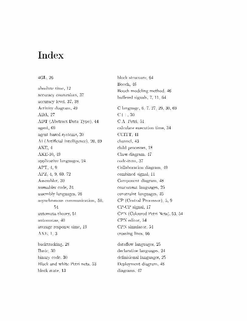
Index
4GL, 26
absolute time, 12
accuracy constraints, 37
accuracy level, 37, 38
Activity diagram, 49
ADA, 27
ADT (Abstract Data Type), 44
agent, 69
agent based systems, 20
AI (Arti�cial Intelligence), 20, 69
AKE, 4
AKE-10, 49
applicative languages, 24
APT, 4, 9
APZ, 4, 9, 69, 72
Assembler, 30
assembler code, 34
assembly languages, 26
asynchronous communication, 50,
54
automata theory, 51
automatas, 40
average response time, 19
AXE, 1, 3
backtracking, 28
Basic, 30
binary code, 30
Black and white Petri nets, 53
block state, 13
block structure, 64
Booch, 46
Booch modeling method, 46
bu�ered signals, 7, 11, 64
C language, 6, 7, 27, 29, 30, 69
C++, 30
C.A. Petri, 51
calculate execution time, 34
CCITT, 41
channel, 43
child processes, 18
Class diagram, 47
code-item, 37
Collaboration diagram, 49
combined signal, 11
Component diagram, 48
concurrent languages, 25
constraint languages, 25
CP (Central Processor), 5, 9
CP-CP signal, 17
CPN (Coloured Petri Nets), 53, 54
CPN editor, 54
CPN simulator, 54
crossing lines, 66
data�ow languages, 25
declarative languages, 24
de�nitional languages, 25
Deployment diagram, 48
diagrams, 47
80 INDEX
direct signals, 7, 11, 64
distributed systems, 44
Dynamic diagrams, 48
Ellemtel, 3
EmuDumpGenTool, 8
EmuTool, 8
Erlang, 27
event counters, 15
event triggered, 19, 69
event triggered languages, 26
executable program, 17
execution e�cient, 14
execution time calculation, 32, 62,
63, 68
Facts Finder, 1, 56, 58, 75
facts-�le, 56, 58
false paths, 32
fault handling, 15
FDL, 40
FDL (Function Description Language),
45
�nding ways, 36
Finite Automata, 40
�ring delays, 53
�ow chars, 40
�ow graph, 33
FORTRAN, 6, 27, 30, 68
fourth generation languages, 26
FP, 27
function oriented concept, 49
functional languages, 24, 25, 27
garbage collection, 71
GCLA, 25
goal-based agents, 21
GOTO-command, 27, 37
Grady Booch, 46
Graph Finder, 39, 56, 62, 74
graphical representation, 39, 69
graphs, 39, 62, 70
GRETA, 1, 39, 40, 56, 70, 72, 74
handling processes, 17
hard real-time system, 19
hardware faults, 15
Haskell, 27
high-level analysis, 32, 34, 70
HL-PLEX, 6, 29, 69
ILP, 58, 70
ILP (Integer Linear Programming),
33
imperative languages, 24
implementation language, 41
initialization signal, 9
intermediate languages, 25
interrupt clock, 13
interrupt handled system, 10
Ivar Jacobson, 46
Java, 1, 66, 72, 73
Jim Rumbaugh, 46
job bu�ers, 10
job table, 12
leaf blocks, 43
LISP, 27
logic languages, 24, 25, 28
loop detection, 35
loop elimination, 36
loop handling, 35
loops, 35
low-level analysis, 32, 34, 70
Lucid, 25
INDEX 81
Mälardalen University, 33
MAS (Maintenance Subsystem), 15
MAU (Maintenance Unit), 5, 15
Mealy machine, 40
message counting, 15
meta languages, 26
ML, 27
modularity, 6, 71
monitors, 15
Moore machine, 40
MS-DOS, 16
MSC (Message Sequence Chart),
50
multiple signal, 11
multitasking, 9
mutual exclusion, 15
Object diagram, 47
object oriented concept, 49
object oriented language, 46
object oriented languages, 26
object oriented system, 22
OMT, 46
OMT (Object Modeling Technique),
46
OOSE, 46
OOSE (Object Oriented Software
Engineering), 46
operating system, 9
optimization, 31, 66
overhead, 18
Pascal, 6, 7, 27, 29, 69
Petri nets, 40, 51, 69
PId (Process Identi�er), 44
places, 51
PLEX, 1, 3, 6, 68
PLEX-compiler, 58
pre-compiler, 31
procedural languages, 24, 26
process, 17
process scheduler, 14
process table, 14, 18
process tree structure, 18
Prolog, 28, 58, 59, 69, 72
PS (Program Store), 7
pseudo-code, 59
Push-Down Automata, 40
query languages, 26
Rational Rose, 49
Rational Software, 46, 49
ready state, 13
real-time system, 72
real-time systems, 6, 19, 44, 69
registers, 17
relative time, 12
RM (Register Memory), 10
RP (Regional Processor), 5, 9
RP-Bus, 5
RP-CP signal, 17
RP-RP signals, 17
RS (Reference Store), 7
running state, 13
scalability, 67
SDL, 1, 40, 54, 70
SDL (Speci�cation and Description
Language), 41
SDL-10, 40, 45, 55, 62, 70
SDT (Signal Distribution Table),
7
semaphores, 15
Sequence diagram, 49
82 INDEX
shared memory, 14
signal entry, 7
signal paradigm, 63
signal route, 43
signal survey, 58
single assignment languages, 25
single signal, 11
soft real-time system, 19, 37
SP (Support Processor), 5
SPC (Stored Program Control), 3
speci�cation language, 41
speci�cation languages, 26
SST (Signal Sending Table), 7
Stack Automata, 40
stack pointer, 17
state elimination, 36
State machine diagram, 48
state machines, 40
Static diagrams, 47
Stochastic Petri nets, 53
Structure Finder, 56, 58, 59
sub-graphs, 39, 65, 70
system calendar, 12
system call, 13
system clock, 16
system load, 16
Televerket, 3
Telia, 3
time accuracy, 16
time constraints, 19
time consuming, 14
time queues, 12
time slicing, 13
Timed Petri nets, 53
timeout value, 20
timesharing system, 17
tokens, 52
tracing, 30
transition �ring, 52
transitions, 51
trap, 13
Turing Machine, 40
UML (Uni�ed Modeling Language),
46
unique signal, 11
UNIX, 16
updating during execution, 15
Use case diagram, 48
VAL, 25
WCET (Worst Case Execution Time),
33
WCETc (Worst Case Execution Time
calculation), 33
Windows, 16
worst case behavior, 32
Attachment I
Prolog code

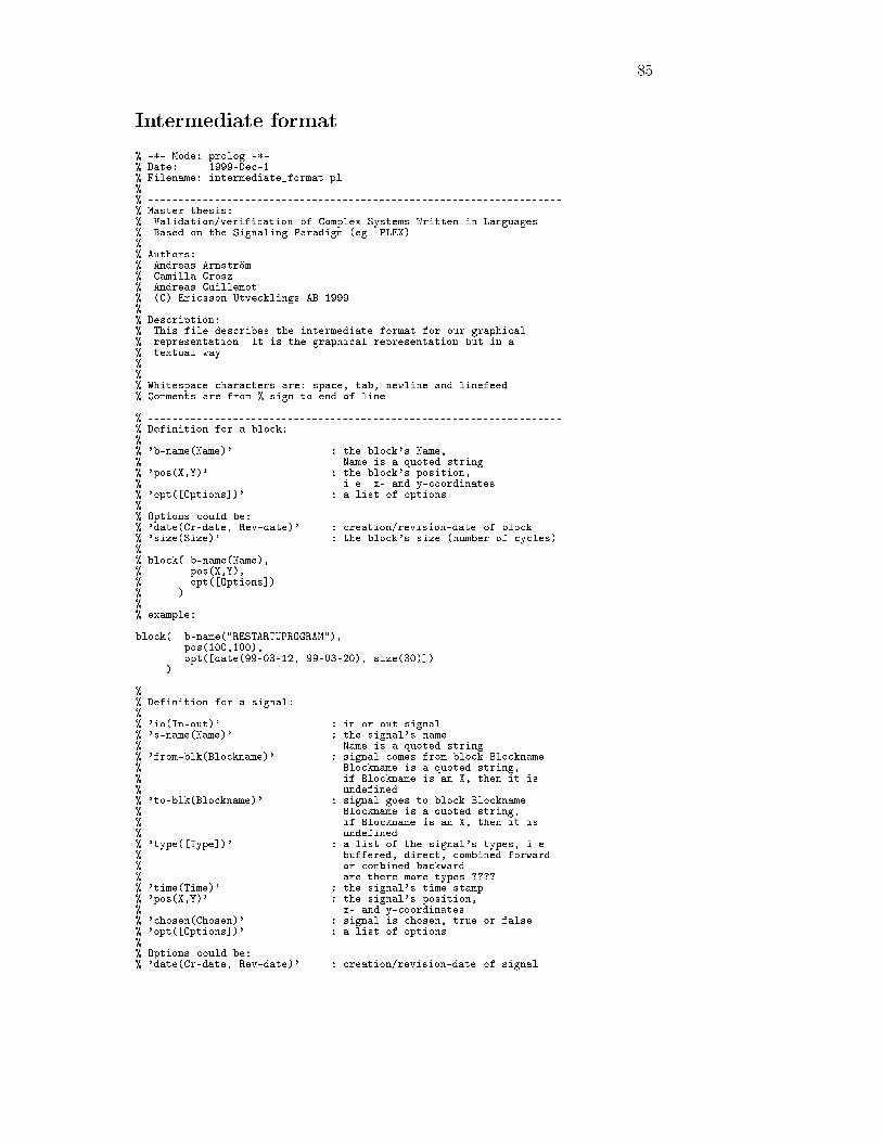
85
Intermediate format
% -*- Mode: prolog -*-% Date: 1999-Dec-1% Filename: intermediate_format.pl%% --------------------------------------------------------------------% Master thesis:% Validation/verification of Complex Systems Written in Languages% Based on the Signaling Paradigm (eg. PLEX)%% Authors:% Andreas Arnström% Camilla Grosz% Andreas Guillemot% (C) Ericsson Utvecklings AB 1999%% Description:% This file describes the intermediate format for our graphical% representation. It is the graphical representation but in a% textual way.%% --------------------------------------------------------------------% Whitespace characters are: space, tab, newline and linefeed.% Comments are from %-sign to end of line.
% --------------------------------------------------------------------% Definition for a block:%% 'b-name(Name)' : the block's Name,% Name is a quoted string% 'pos(X,Y)' : the block's position,% i.e. x- and y-coordinates% 'opt([Options])' : a list of options%% Options could be:% 'date(Cr-date, Rev-date)' : creation/revision-date of block% 'size(Size)' : the block's size (number of cycles)%% block( b-name(Name),% pos(X,Y),% opt([Options])% ).%% example:
block( b-name("RESTARTUPROGRAM"),pos(100,100),opt([date(99-03-12, 99-03-20), size(30)])
).
% --------------------------------------------------------------------% Definition for a signal:%% 'io(In-out)' : in or out signal% 's-name(Name)' : the signal's name% Name is a quoted string% 'from-blk(Blockname)' : signal comes from block Blockname% Blockname is a quoted string,% if Blockname is an X, then it is% undefined% 'to-blk(Blockname)' : signal goes to block Blockname% Blockname is a quoted string,% if Blockname is an X, then it is% undefined% 'type([Type])' : a list of the signal's types, i.e.% buffered, direct, combined forward% or combined backward% are there more types ????% 'time(Time)' : the signal's time stamp% 'pos(X,Y)' : the signal's position,% x- and y-coordinates% 'chosen(Chosen)' : signal is chosen, true or false% 'opt([Options])' : a list of options%% Options could be:% 'date(Cr-date, Rev-date)' : creation/revision-date of signal
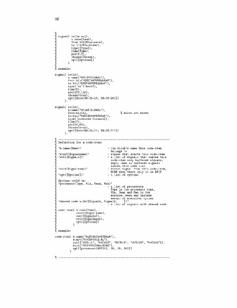
86
%% signal( io(In-out),% s-name(Name),% from-blk(Blockname),% to-blk(Blockname),% type([Type]),% time(Time),% pos(X,Y),% chosen(Chosen),% opt([Options])% ).%% example:
signal( io(in),s-name("MYCOPYSIGNAL"),from-blk("RESTARTUPROGRAM"),to-blk("RESTARTUPROGRAM"),type([call-back]),time(5),pos(150,150),chosen(true),opt([date(99-03-13, 99-03-20)])
).
signal( io(in),s-name("MYTESTSIGNAL"),from-blk(X), % Block not knownto-blk("RESTARTUPROGRAM"),type([combined-forward]),time(7),pos(50,50),chosen(true),opt([date(99-03-14, 99-03-21)])
).
% --------------------------------------------------------------------% Definition for a code-item:%% 'b-name(Name)' : the block's name this code-item% belongs to% 'start(Signalname)' : signal that starts this code-item% 'out([Signals])' : a list of signals that leaves this% code-item only buffered signals,% empty when no buffered signals% leaves this code-item% 'exit(Signalname)' : direct signal from this code-item,% NONE when there only is an EXIT.% 'opt([Options])' : a list of options%% Options could be:% 'processor(Type, Min, Mean, Max)'% : a list of processors% Type is the processor type,% Min, Mean and Max is the% minimum, mean and maximum% amount of execution cycles% 'shared-code-with([SignalA, SignalX, ...])'% : a list of signals with shared code%% code-item( b-name(Name),% start(Signalname),% out([Signals]),% exit(Signalname),% opt([Options])% ).%% example:
code-item( b-name("RESTARTUPROGRAM"),start("MYCOPYSIGNAL"),out(["MYOUT1", "MYOUT2", "MYOUT3", "MYOUT4", "MYOUT5"]),exit("MYCOPYSIGNALDONE"),opt([processor(APZ212, 30, 45, 60)])
).
% --------------------------------------------------------------------
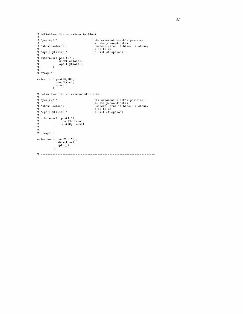
87
% Definition for an extern-in block:%% 'pos(X,Y)' : the external block's position,% x- and y-coordinates% 'show(Boolean)' : Boolean ,true if block is shown,% else false% 'opt([Options])' : a list of options%% extern-in( pos(X,Y),% show(Boolean),% opt([Options])% ).%% example:
extern-in( pos(10,10),show(true),opt([])
).
% Definition for an extern-out block:%% 'pos(X,Y)' : the external block's position,% x- and y-coordinates% 'show(Boolean)' : Boolean ,true if block is shown,% else false% 'opt([Options])' : a list of options%% extern-out( pos(X,Y),% show(Boolean),% opt([Options])% ).%% example:
extern-out( pos(200,10),show(true),opt([])
).
% --------------------------------------------------------------------
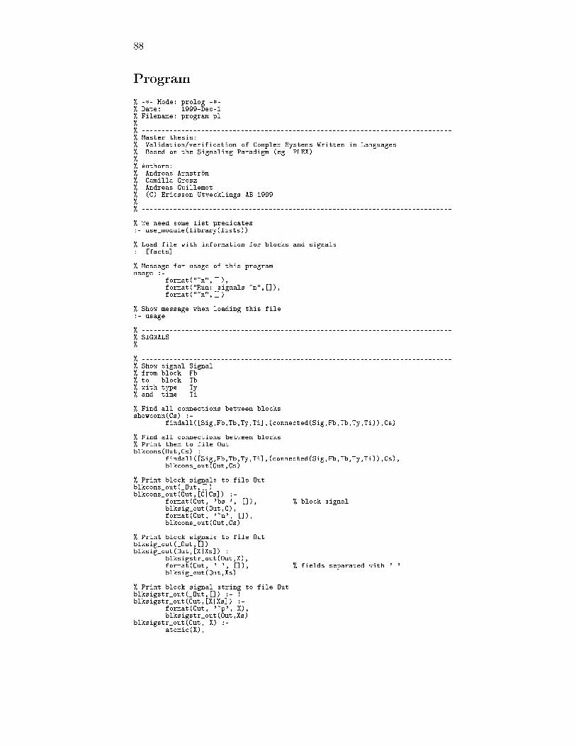
88
Program
% -*- Mode: prolog -*-% Date: 1999-Dec-1% Filename: program.pl%% ------------------------------------------------------------------------------% Master thesis:% Validation/verification of Complex Systems Written in Languages% Based on the Signaling Paradigm (eg. PLEX)%% Authors:% Andreas Arnström% Camilla Grosz% Andreas Guillemot% (C) Ericsson Utvecklings AB 1999%% ------------------------------------------------------------------------------
% We need some list predicates.:- use_module(library(lists)).
% Load file with information for blocks and signals.:- [facts].
% Message for usage of this program.usage :-
format("~n",[]),format("Run: signals.~n",[]),format("~n",[]).
% Show message when loading this file.:- usage.
% ------------------------------------------------------------------------------% SIGNALS%
% ------------------------------------------------------------------------------% Show signal Signal% from block Fb% to block Tb% with type Ty% and time Ti
% Find all connections between blocksshowconn(Cs) :-
findall([Sig,Fb,Tb,Ty,Ti],(connected(Sig,Fb,Tb,Ty,Ti)),Cs).
% Find all connections between blocks% Print them to file Outblkcons(Out,Cs) :-
findall([Sig,Fb,Tb,Ty,Ti],(connected(Sig,Fb,Tb,Ty,Ti)),Cs),blkcons_out(Out,Cs).
% Print block signals to file Outblkcons_out(_Out,[]).blkcons_out(Out,[C|Cs]) :-
format(Out, 'bs.', []), % block signalblksig_out(Out,C),format(Out, '~n', []),blkcons_out(Out,Cs).
% Print block signals to file Outblksig_out(_Out,[]).blksig_out(Out,[X|Xs]) :-
blksigstr_out(Out,X),format(Out, '.', []), % fields separated with '.'blksig_out(Out,Xs).
% Print block signal string to file Outblksigstr_out(_Out,[]) :- !.blksigstr_out(Out,[X|Xs]) :-
format(Out, '~p', X),blksigstr_out(Out,Xs).
blksigstr_out(Out, X) :-atomic(X),
89
format(Out, '~p', X).
% ------------------------------------------------------------------------------% BLOCKS%
% Find all blocks% showblks(+Out,-Bs)showblks(Out,Bs) :-
findall([Bn],(blkname(Bn)),Bs),blk_out(Out,Bs).
% Find a block with name Bn% blkname(-Bn)blkname(Bn) :-
block(b_name(Bn),_,_).
% Print blocknames to file Out% blk_out(+Out,+Bs)blk_out(_Out,[]).blk_out(Out,[B|Bs]) :-
format(Out, 'bl.', []), % blocksblkname_out(Out,B),format(Out, '~n', []),blk_out(Out,Bs).
% Create file with block's name% blkname_out(+Out,+Bs)blkname_out(_Out,[]) :- !.blkname_out(Out,[B|Bs]) :-
format(Out, '~p.', B),open_bn_file(B, Bout), % Print to file with block's nameshowcis(Bout,B), % Code-items for every blockclose_file(Bout),blknamestr_out(Out,Bs).
blkname_out(Out, B) :-atomic(B),format(Out, '~p.', B),open_bn_file(B, Bout), % Print to file with block's nameshowcis(Bout,B), % Code-items for every blockformat(Bout, '~p.', B),close_file(Bout).
% Print block name string to file Out% blknamestr_out(+Out,+Bs)blknamestr_out(_Out,[]) :- !.blknamestr_out(Out,[B|Bs]) :-
format(Out, '~p', B),blknamestr_out(Out,Bs).
blknamestr_out(Out, B) :-atomic(B),format(Out, '~p', B).
% ------------------------------------------------------------------------------% CONNECTIONS%
% Find a% signal Sig% from Fb% to Tb% connected(?Sig,-Fromblk,-Toblk)connected(Sig,Fb,Tb) :-
signal(io(in),Sig,_,Tb,_,_,_,_,_),signal(io(out),Sig,Fb,_,_,_,_,_,_).
% Find a% signal Sig% from block Fb% to block Tb% with type Ty% and time Ti% connected(?Sig,-Fromblk,-Toblk,-Type)connected(Sig,Fb,Tb,Ty) :-
signal( io(out),s_name(Sig),
90
from_blk(Fb),_,type(Ty),_,_,_,_).
connected(Sig,Fb,extern_out,Ty) :-signal( io(out),
s_name(Sig),from_blk(Fb),to_blk(extern_out),type(Ty),_,_,_,_).
% Find a% signal Sig% from block Fb% to block Tb% with type Ty% and time Ti% connected(?Sig,-Fromblk,-Toblk,-Type,-Time)connected(Sig,Fb,Tb,Ty,Ti) :-
signal( io(in),s_name(Sig),_,to_blk(Tb),_,_,_,_,_),
signal( io(out),s_name(Sig),from_blk(Fb),_,type(Ty),time(Ti),_,_,_).
connected(Sig,Fb,extern_out,Ty,Ti) :-signal(io(out),
s_name(Sig),from_blk(Fb),to_blk(extern_out),type(Ty),time(Ti),_,_,_).
% ------------------------------------------------------------------------------% CODE-ITEMS%
% Find all code-items for block Bn and print their information to file Out% showcis(+Out,+Bn)showcis(Out,Bn) :-
findall([Bn,Ss],code_item(b_name(Bn),start(Ss),_,_,_),CIs),cis_out(Out,CIs), % print code-itemsciis_out(Out,Bn). % print code-item signals
% Find all connections between code items for a given signal Sig% findciconn(-Codeitemconnections,+Sig,+Fromcodeitem)findciconn(Cics,Sig,Fci) :-
findall([Fci,Tci,Ty,Ti],(connected(Sig,Fci,Tci,Ty,Ti)),Cics).
% Print code-items to file Out% cis_out(+Out,+Codeitems)cis_out(_Out,[]).cis_out(Out,[C|Cs]) :-
format(Out, 'ci.', []), % code-itemscissig_out(Out,C), % code-item signalsformat(Out, '~n', []),cis_out(Out,Cs).
% Print code-item signals to file Out% cissig_out(+Out,+Codeitemsignals)cissig_out(_Out,[]) :- !.cissig_out(Out,[B|Bs]) :-
is_list(B),cissig_out(Out,B),cissig_out(Out,Bs).
cissig_out(Out,[B|Bs]) :-
91
atomic(B),format(Out, '~p.', B),cissig_out(Out,Bs).
cissig_out(Out, B) :-atomic(B),format(Out, '~p.', B).
% Print code-item signals to file Out% cissig_out(+Out,+Codeitemsignals,+Blockname)cissig_out(_Out,[],_) :- !.cissig_out(Out,[[B]|Bs],Bn) :-
cissig_out(Out,B,Bn),cissig_out(Out,Bs,Bn).
cissig_out(Out,[B|Bs],Bn) :-atomic(B),findciconn(Cics,B,Bn),format(Out, 'is.',[]), % code-item signalformat(Out, '~p.', Bn), % print block nameformat(Out, '~p.', B), % print signal namecissig_out(Out,Cics), % print conn, type, timeformat(Out, '~n',[]),cissig_out(Out,Bs,Bn).
cissig_out(Out,B,_) :-atomic(B),format(Out, '~p.', B).
% Print code-item item signals to file Out% ciis_out(+Out,+Blockname)ciis_out(Out,Bn) :-
findall([Os],code_item(b_name(Bn),_,out(Os),_,_),CIs),cissig_out(Out,CIs,Bn).
% ------------------------------------------------------------------------------% SYSTEM%
% Open the file for blocks and signal information% open_bs_file(-Filehandle)open_bs_file(X) :-
open('output/blocksignal.txt', write, X).
% Open file with blocks name% open_bn_file(+Blockname,-Filehadle)open_bn_file(Bn,X) :-
atom_chars('output/',Dir),atom_chars(Bn,Bnt),append(Dir,Bnt,Out),atom_chars(File,Out),open(File, write, X).
% Close filehandle% close_file(+Filehandle)close_file(X) :-
format(X,'~n',[]),close(X).
% This is the programsignals :-
open_bs_file(File),showblks(File,_Blocks), % Print block informationblkcons(File,_Connections), % Print block connectionsclose_file(File).
% Run the program when file is loaded.:- signals.
% append is in module library(lists)% append([],Ys,Ys).% append([X|Xs],Ys,[X|Zs]) :-% append(Xs,Ys,Zs).% ------------------------------------------------------------------------------
92
Facts
% -*- Mode: prolog -*-% Date: 1999-Dec-1% Filename: facts.pl%% ------------------------------------------------------------------------------% Master thesis:% Validation/verification of Complex Systems Written in Languages% Based on the Signaling Paradigm (eg. PLEX)%% Authors:% Andreas Arnström% Camilla Grosz% Andreas Guillemot% (C) Ericsson Utvecklings AB 1999%% ------------------------------------------------------------------------------
block( b_name('MYBLOCK1'),pos(X,Y),opt([date(99-03-12, 99-03-20), size(30)])
).
block( b_name('MYBLOCK2'),pos(X,Y),opt([date(99-03-12, 99-03-20), size(30)])
).
block( b_name('MYBLOCK3'),pos(X,Y),opt([date(99-03-12, 99-03-20), size(30)])
).
block( b_name('MYBLOCK4'),pos(X,Y),opt([date(99-03-12, 99-03-20), size(30)])
).
block( b_name('MYBLOCK5'),pos(X,Y),opt([date(99-03-12, 99-03-20), size(30)])
).
from_blk(extern_in).from_blk('MYBLOCK1').from_blk('MYBLOCK2').from_blk('MYBLOCK3').from_blk('MYBLOCK4').from_blk('MYBLOCK5').
to_blk(extern_out).to_blk('MYBLOCK1').to_blk('MYBLOCK2').to_blk('MYBLOCK3').to_blk('MYBLOCK4').to_blk('MYBLOCK5').
% ------------------------------------------------------------------------------% Signals
s_name('MYSIGNAL1').s_name('MYSIGNAL2').s_name('MYSIGNAL3').s_name('MYSIGNAL4').s_name('MYSIGNAL5').s_name('DONTKNOW').
% ------------------------------------------------------------------------------% Signals in
signal( io(in),s_name('MYSIGNAL1'),from_blk(Fblk),to_blk('MYBLOCK1'),type([Type1]),time(Time),
93
pos(X,Y),chosen(true),opt([date(99-03-13, 99-03-20)])
).
signal( io(in),s_name('MYSIGNAL2'),from_blk(Fblk),to_blk('MYBLOCK2'),type([Type1]),time(Time),pos(X,Y),chosen(true),opt([date(99-03-13, 99-03-20)])
).
signal( io(in),s_name('MYSIGNAL3'),from_blk(Fblk),to_blk('MYBLOCK3'),type([Type1]),time(Time),pos(X,Y),chosen(true),opt([date(99-03-13, 99-03-20)])
).
signal( io(in),s_name('MYSIGNAL4'),from_blk(Fblk),to_blk('MYBLOCK4'),type([Type1]),time(Time),pos(X,Y),chosen(true),opt([date(99-03-13, 99-03-20)])
).
signal( io(in),s_name('MYSIGNAL5'),from_blk(Fblk),to_blk('MYBLOCK5'),type([Type1]),time(Time),pos(X,Y),chosen(true),opt([date(99-03-13, 99-03-20)])
).
% ------------------------------------------------------------------------------% Signals out
signal( io(out),s_name('MYSIGNAL1'),from_blk(extern_in),to_blk('MYBLOCK1'),type([buffered]),time(0),pos(X,Y),chosen(true),opt([date(99-03-13, 99-03-20)])
).
signal( io(out),s_name('MYSIGNAL2'),from_blk(extern_in),to_blk('MYBLOCK2'),type([buffered]),time(0),pos(X,Y),chosen(true),opt([date(99-03-13, 99-03-20)])
).
signal( io(out),s_name('MYSIGNAL3'),from_blk(extern_in),
94
to_blk('MYBLOCK3'),type([buffered]),time(0),pos(X,Y),chosen(true),opt([date(99-03-13, 99-03-20)])
).
signal( io(out),s_name('MYSIGNAL4'),from_blk(extern_in),to_blk('MYBLOCK4'),type([buffered]),time(0),pos(X,Y),chosen(true),opt([date(99-03-13, 99-03-20)])
).
signal( io(out),s_name('MYSIGNAL5'),from_blk(extern_in),to_blk('MYBLOCK5'),type([buffered]),time(0),pos(X,Y),chosen(true),opt([date(99-03-13, 99-03-20)])
).
signal( io(out),s_name('MYSIGNAL1'),from_blk('MYBLOCK4'),to_blk('MYBLOCK1'),type([direct]),time(5),pos(X,Y),chosen(true),opt([date(99-03-13, 99-03-20)])
).
signal( io(out),s_name('MYSIGNAL2'),from_blk('MYBLOCK1'),to_blk('MYBLOCK2'),type([direct]),time(5),pos(X,Y),chosen(true),opt([date(99-03-13, 99-03-20)])
).
signal( io(out),s_name('MYSIGNAL2'),from_blk('MYBLOCK3'),to_blk('MYBLOCK2'),type([buffered]),time(5),pos(X,Y),chosen(true),opt([date(99-03-13, 99-03-20)])
).
signal( io(out),s_name('MYSIGNAL3'),from_blk('MYBLOCK1'),to_blk('MYBLOCK3'),type([buffered]),time(5),pos(X,Y),chosen(true),opt([date(99-03-13, 99-03-20)])
).
signal( io(out),s_name('MYSIGNAL3'),from_blk('MYBLOCK5'),
95
to_blk('MYBLOCK3'),type([direct]),time(5),pos(X,Y),chosen(true),opt([date(99-03-13, 99-03-20)])
).
signal( io(out),s_name('MYSIGNAL4'),from_blk('MYBLOCK2'),to_blk('MYBLOCK4'),type([buffered]),time(5),pos(X,Y),chosen(true),opt([date(99-03-13, 99-03-20)])
).
signal( io(out),s_name('MYSIGNAL5'),from_blk('MYBLOCK1'),to_blk('MYBLOCK5'),type([buffered]),time(5),pos(X,Y),chosen(true),opt([date(99-03-13, 99-03-20)])
).
signal( io(out),s_name('MYSIGNAL5'),from_blk('MYBLOCK3'),to_blk('MYBLOCK5'),type([direct]),time(5),pos(X,Y),chosen(true),opt([date(99-03-13, 99-03-20)])
).
signal( io(out),s_name('DONTKNOW'),from_blk('MYBLOCK4'),to_blk(extern_out),type([buffered]),time(5),pos(X,Y),chosen(true),opt([date(99-03-13, 99-03-20)])
).
signal( io(out),s_name('DONTKNOW'),from_blk('MYBLOCK5'),to_blk(extern_out),type([buffered]),time(5),pos(X,Y),chosen(true),opt([date(99-03-13, 99-03-20)])
).
% ------------------------------------------------------------------------------% code_items
code_item( b_name('MYBLOCK1'),start('MYSIGNAL1'),out(['MYSIGNAL2', 'MYSIGNAL3', 'MYSIGNAL5']),exit('MYSIGNAL2'),opt([processor(APZ212, 30, 45, 60)])
).
code_item( b_name('MYBLOCK1'),start('MYSIGNAL1_I'),out(['MYSIGNAL2']),exit('MYSIGNAL2'),
96
opt([processor(APZ212, 30, 45, 60)])).
code_item( b_name('MYBLOCK2'),start('MYSIGNAL2'),out(['MYSIGNAL4']),exit(none),opt([processor(APZ212, 30, 45, 60)])
).
code_item( b_name('MYBLOCK3'),start('MYSIGNAL3'),out(['MYSIGNAL2', 'MYSIGNAL5']),exit('MYSIGNAL5'),opt([processor(APZ212, 30, 45, 60)])
).
code_item( b_name('MYBLOCK4'),start('MYSIGNAL4'),out(['MYSIGNAL1', 'DONTKNOW']),exit('MYSIGNAL1'),opt([processor(APZ212, 30, 45, 60)])
).
code_item( b_name('MYBLOCK5'),start('MYSIGNAL5'),out(['MYSIGNAL3', 'DONTKNOW']),exit('MYSIGNAL3'),opt([processor(APZ212, 30, 45, 60)])
).
code_item( b_name(extern_in),start(none),out(['MYSIGNAL1','MYSIGNAL2','MYSIGNAL3','MYSIGNAL4','MYSIGNAL5']),exit(none),opt([processor(APZ212, 30, 45, 60)])
).
code_item( b_name(extern_out),start('DONTKNOW'),out([]),exit(none),opt([processor(APZ212, 30, 45, 60)])
).
% ------------------------------------------------------------------------------% External block in
extern_in( pos(X,Y),show(true),opt([])
).
% ------------------------------------------------------------------------------% External block out
extern_out( pos(X,Y),show(true),opt([])
).
Attachment II
Java code


99
Graph Finder
import java.awt.*;import java.awt.event.*;
/******************************************************Class "GraphFinder"******************************************************/public class GraphFinder{/*******void main*******//***********************/public static void main(String[] args){
GraphFinderFrame frame = new GraphFinderFrame();frame.show();
}}
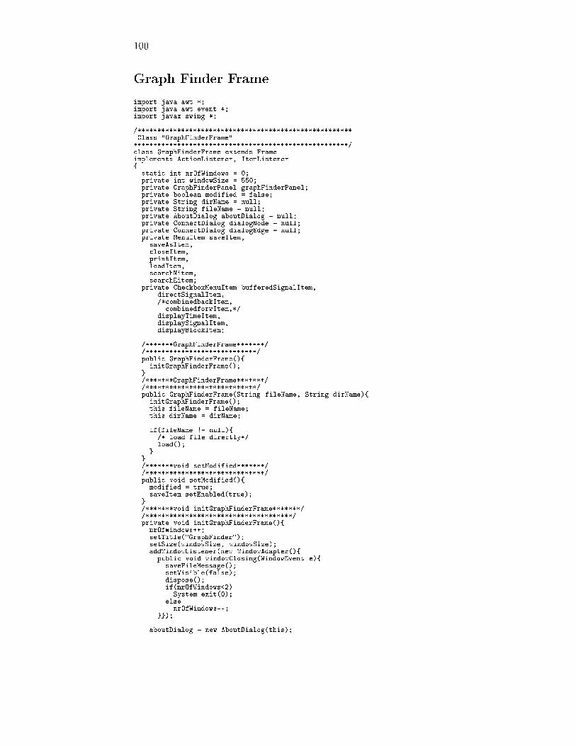
100
Graph Finder Frame
import java.awt.*;import java.awt.event.*;import javax.swing.*;
/******************************************************Class "GraphFinderFrame"******************************************************/class GraphFinderFrame extends Frameimplements ActionListener, ItemListener{
static int nrOfWindows = 0;private int windowSize = 550;private GraphFinderPanel graphFinderPanel;private boolean modified = false;private String dirName = null;private String fileName = null;private AboutDialog aboutDialog = null;private ConnectDialog dialogNode = null;private ConnectDialog dialogEdge = null;private MenuItem saveItem,
saveAsItem,closeItem,printItem,loadItem,searchNitem,searchEitem;
private CheckboxMenuItem bufferedSignalItem,directSignalItem,/*combinedbackItem,combinedforwItem,*/
displayTimeItem,displaySignalItem,displayBlockItem;
/*******GraphFinderFrame*******//****************************/public GraphFinderFrame(){
initGraphFinderFrame();}/*******GraphFinderFrame*******//****************************/public GraphFinderFrame(String fileName, String dirName){
initGraphFinderFrame();this.fileName = fileName;this.dirName = dirName;
if(fileName != null){/* load file directly*/load();
}}/*******void setModified*******//******************************/public void setModified(){
modified = true;saveItem.setEnabled(true);
}/*******void initGraphFinderFrame*******//*************************************/private void initGraphFinderFrame(){
nrOfWindows++;setTitle("GraphFinder");setSize(windowSize, windowSize);addWindowListener(new WindowAdapter(){
public void windowClosing(WindowEvent e){saveFileMessage();setVisible(false);dispose();if(nrOfWindows<2)
System.exit(0);else
nrOfWindows--;}});
aboutDialog = new AboutDialog(this);
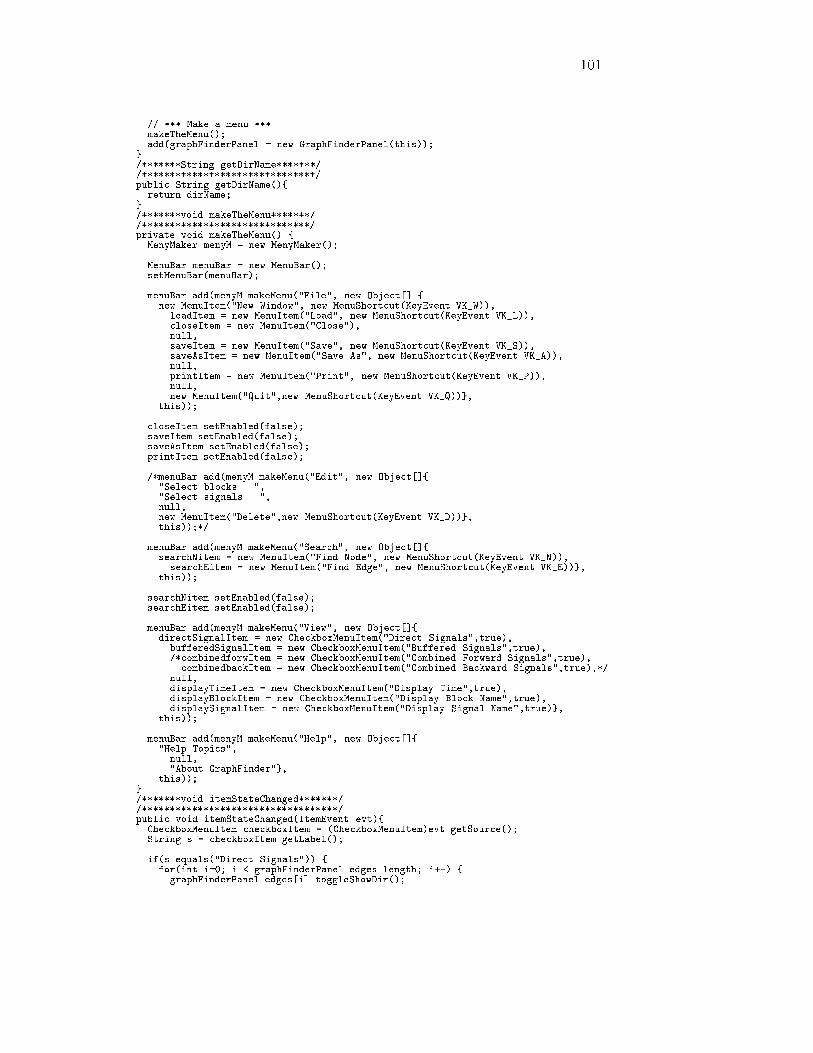
101
// *** Make a menu ***makeTheMenu();add(graphFinderPanel = new GraphFinderPanel(this));
}/*******String getDirName*******//*******************************/public String getDirName(){
return dirName;}/*******void makeTheMenu*******//******************************/private void makeTheMenu() {
MenyMaker menyM = new MenyMaker();
MenuBar menuBar = new MenuBar();setMenuBar(menuBar);
menuBar.add(menyM.makeMenu("File", new Object[] {new MenuItem("New Window", new MenuShortcut(KeyEvent.VK_W)),
loadItem = new MenuItem("Load", new MenuShortcut(KeyEvent.VK_L)),closeItem = new MenuItem("Close"),null,saveItem = new MenuItem("Save", new MenuShortcut(KeyEvent.VK_S)),saveAsItem = new MenuItem("Save As", new MenuShortcut(KeyEvent.VK_A)),null,printItem = new MenuItem("Print", new MenuShortcut(KeyEvent.VK_P)),null,new MenuItem("Quit",new MenuShortcut(KeyEvent.VK_Q))},
this));
closeItem.setEnabled(false);saveItem.setEnabled(false);saveAsItem.setEnabled(false);printItem.setEnabled(false);
/*menuBar.add(menyM.makeMenu("Edit", new Object[]{"Select blocks...","Select signals...",null,new MenuItem("Delete",new MenuShortcut(KeyEvent.VK_D))},this));*/
menuBar.add(menyM.makeMenu("Search", new Object[]{searchNitem = new MenuItem("Find Node", new MenuShortcut(KeyEvent.VK_N)),
searchEitem = new MenuItem("Find Edge", new MenuShortcut(KeyEvent.VK_E))},this));
searchNitem.setEnabled(false);searchEitem.setEnabled(false);
menuBar.add(menyM.makeMenu("View", new Object[]{directSignalItem = new CheckboxMenuItem("Direct Signals",true),
bufferedSignalItem = new CheckboxMenuItem("Buffered Signals",true),/*combinedforwItem = new CheckboxMenuItem("Combined Forward Signals",true),
combinedbackItem = new CheckboxMenuItem("Combined Backward Signals",true),*/null,displayTimeItem = new CheckboxMenuItem("Display Time",true),displayBlockItem = new CheckboxMenuItem("Display Block Name",true),displaySignalItem = new CheckboxMenuItem("Display Signal Name",true)},
this));
menuBar.add(menyM.makeMenu("Help", new Object[]{"Help Topics",
null,"About GraphFinder"},
this));}/*******void itemStateChanged*******//***********************************/public void itemStateChanged(ItemEvent evt){
CheckboxMenuItem checkboxItem = (CheckboxMenuItem)evt.getSource();String s = checkboxItem.getLabel();
if(s.equals("Direct Signals")) {for(int i=0; i < graphFinderPanel.edges.length; i++) {
graphFinderPanel.edges[i].toggleShowDir();
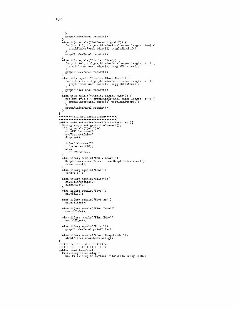
102
}graphFinderPanel.repaint();
}else if(s.equals("Buffered Signals")) {
for(int i=0; i < graphFinderPanel.edges.length; i++) {graphFinderPanel.edges[i].toggleShowBuf();
}graphFinderPanel.repaint();
}else if(s.equals("Display Time")) {
for(int i=0; i < graphFinderPanel.edges.length; i++) {graphFinderPanel.edges[i].toggleShowTime();
}graphFinderPanel.repaint();
}else if(s.equals("Display Block Name")) {
for(int i=0; i < graphFinderPanel.nodes.length; i++) {graphFinderPanel.nodes[i].toggleShowName();
}graphFinderPanel.repaint();
}else if(s.equals("Display Signal Name")) {
for(int i=0; i < graphFinderPanel.edges.length; i++) {graphFinderPanel.edges[i].toggleShowName();
}graphFinderPanel.repaint();
}}/*******void actionPerformed*******//**********************************/public void actionPerformed(ActionEvent evt){
String arg = evt.getActionCommand();if(arg.equals("Quit")){
saveFileMessage();setVisible(false);dispose();
if(nrOfWindows<2)System.exit(0);
elsenrOfWindows--;
}else if(arg.equals("New Window")){
GraphFinderFrame frame = new GraphFinderFrame();frame.show();
}else if(arg.equals("Load"))
loadFile();
else if(arg.equals("Close")){saveFileMessage();closeFile();
}else if(arg.equals("Save"))
saveFile();
else if(arg.equals("Save As"))saveFileAs();
else if(arg.equals("Find Node"))searchNode();
else if(arg.equals("Find Edge"))searchEdge();
else if(arg.equals("Print"))graphFinderPanel.printFile();
else if(arg.equals("About GraphFinder"))aboutDialog.showAboutDialog();
}/*******void loadFile*******//***************************/public void loadFile(){
FileDialog fileDialog =new FileDialog(this,"Load File",FileDialog.LOAD);
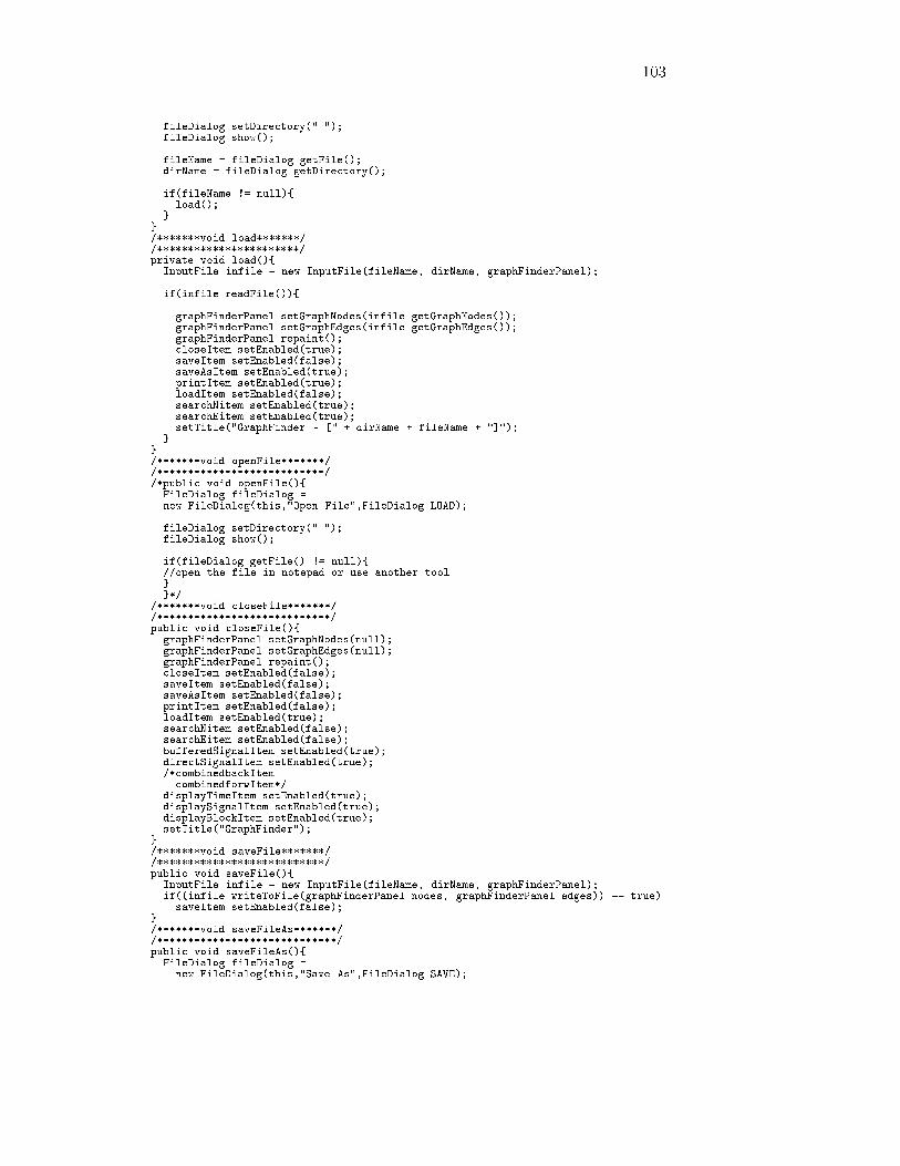
103
fileDialog.setDirectory(".");fileDialog.show();
fileName = fileDialog.getFile();dirName = fileDialog.getDirectory();
if(fileName != null){load();
}}/*******void load*******//***********************/private void load(){
InputFile infile = new InputFile(fileName, dirName, graphFinderPanel);
if(infile.readFile()){
graphFinderPanel.setGraphNodes(infile.getGraphNodes());graphFinderPanel.setGraphEdges(infile.getGraphEdges());graphFinderPanel.repaint();closeItem.setEnabled(true);saveItem.setEnabled(false);saveAsItem.setEnabled(true);printItem.setEnabled(true);loadItem.setEnabled(false);searchNitem.setEnabled(true);searchEitem.setEnabled(true);setTitle("GraphFinder - [" + dirName + fileName + "]");
}}/*******void openFile*******//***************************//*public void openFile(){
FileDialog fileDialog =new FileDialog(this,"Open File",FileDialog.LOAD);
fileDialog.setDirectory(".");fileDialog.show();
if(fileDialog.getFile() != null){//open the file in notepad or use another tool}}*/
/*******void closeFile*******//****************************/public void closeFile(){
graphFinderPanel.setGraphNodes(null);graphFinderPanel.setGraphEdges(null);graphFinderPanel.repaint();closeItem.setEnabled(false);saveItem.setEnabled(false);saveAsItem.setEnabled(false);printItem.setEnabled(false);loadItem.setEnabled(true);searchNitem.setEnabled(false);searchEitem.setEnabled(false);bufferedSignalItem.setEnabled(true);directSignalItem.setEnabled(true);/*combinedbackItem
combinedforwItem*/displayTimeItem.setEnabled(true);displaySignalItem.setEnabled(true);displayBlockItem.setEnabled(true);setTitle("GraphFinder");
}/*******void saveFile*******//***************************/public void saveFile(){
InputFile infile = new InputFile(fileName, dirName, graphFinderPanel);if((infile.writeToFile(graphFinderPanel.nodes, graphFinderPanel.edges)) == true)
saveItem.setEnabled(false);}/*******void saveFileAs*******//*****************************/public void saveFileAs(){
FileDialog fileDialog =new FileDialog(this,"Save As",FileDialog.SAVE);
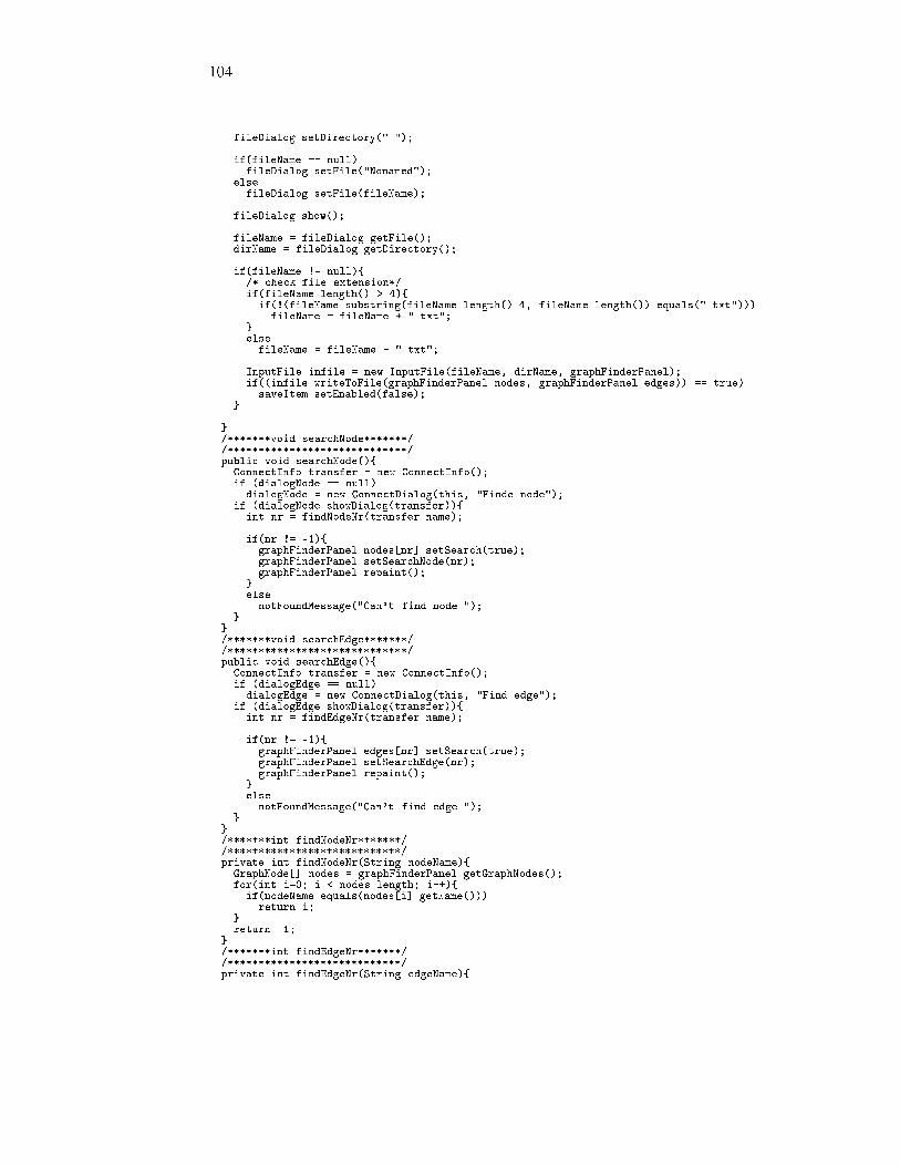
104
fileDialog.setDirectory(".");
if(fileName == null)fileDialog.setFile("Nonamed");
elsefileDialog.setFile(fileName);
fileDialog.show();
fileName = fileDialog.getFile();dirName = fileDialog.getDirectory();
if(fileName != null){/* check file extension*/if(fileName.length() > 4){if(!(fileName.substring(fileName.length()-4, fileName.length()).equals(".txt")))
fileName = fileName + ".txt";}elsefileName = fileName + ".txt";
InputFile infile = new InputFile(fileName, dirName, graphFinderPanel);if((infile.writeToFile(graphFinderPanel.nodes, graphFinderPanel.edges)) == true)saveItem.setEnabled(false);
}
}/*******void searchNode*******//*****************************/public void searchNode(){
ConnectInfo transfer = new ConnectInfo();if (dialogNode == null)
dialogNode = new ConnectDialog(this, "Finde node");if (dialogNode.showDialog(transfer)){
int nr = findNodeNr(transfer.name);
if(nr != -1){graphFinderPanel.nodes[nr].setSearch(true);graphFinderPanel.setSearchNode(nr);graphFinderPanel.repaint();
}elsenotFoundMessage("Can't find node.");
}}/*******void searchEdge*******//*****************************/public void searchEdge(){
ConnectInfo transfer = new ConnectInfo();if (dialogEdge == null)
dialogEdge = new ConnectDialog(this, "Find edge");if (dialogEdge.showDialog(transfer)){
int nr = findEdgeNr(transfer.name);
if(nr != -1){graphFinderPanel.edges[nr].setSearch(true);graphFinderPanel.setSearchEdge(nr);graphFinderPanel.repaint();
}elsenotFoundMessage("Can't find edge.");
}}/*******int findNodeNr*******//****************************/private int findNodeNr(String nodeName){GraphNode[] nodes = graphFinderPanel.getGraphNodes();for(int i=0; i < nodes.length; i++){
if(nodeName.equals(nodes[i].getName()))return i;
}return -1;
}/*******int findEdgeNr*******//****************************/private int findEdgeNr(String edgeName){
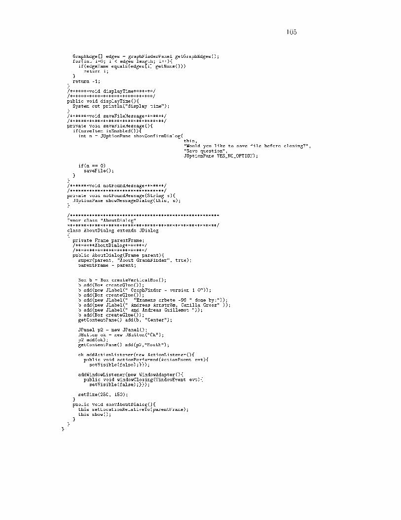
105
GraphEdge[] edges = graphFinderPanel.getGraphEdges();for(int i=0; i < edges.length; i++){
if(edgeName.equals(edges[i].getName()))return i;
}return -1;
}/*******void displayTime*******//******************************/public void displayTime(){
System.out.println("display time");}/*******void saveFileMessage*******//**********************************/private void saveFileMessage(){
if(saveItem.isEnabled()){int n = JOptionPane.showConfirmDialog(
this,"Would you like to save file before closing?","Save question",JOptionPane.YES_NO_OPTION);
if(n == 0)saveFile();
}}/*******void notFoundMessage*******//**********************************/private void notFoundMessage(String s){
JOptionPane.showMessageDialog(this, s);}
/******************************************************Inner class "AboutDialog"******************************************************/class AboutDialog extends JDialog{
private Frame parentFrame;/*******AboutDialog*******//*************************/public AboutDialog(Frame parent){
super(parent, "About GraphFinder", true);parentFrame = parent;
Box b = Box.createVerticalBox();b.add(Box.createGlue());b.add(new JLabel(" GraphFinder - version 1.0"));b.add(Box.createGlue());b.add(new JLabel(" \"Examens arbete -99\" done by:"));b.add(new JLabel(" Andreas Arnström, Camilla Grosz" ));b.add(new JLabel(" and Andreas Guillemot."));b.add(Box.createGlue());getContentPane().add(b, "Center");
JPanel p2 = new JPanel();JButton ok = new JButton("Ok");p2.add(ok);getContentPane().add(p2,"South");
ok.addActionListener(new ActionListener(){public void actionPerformed(ActionEvent evt){setVisible(false);}});
addWindowListener(new WindowAdapter(){public void windowClosing(WindowEvent evt){setVisible(false);}});
setSize(250, 150);}public void showAboutDialog(){
this.setLocationRelativeTo(parentFrame);this.show();
}}
}
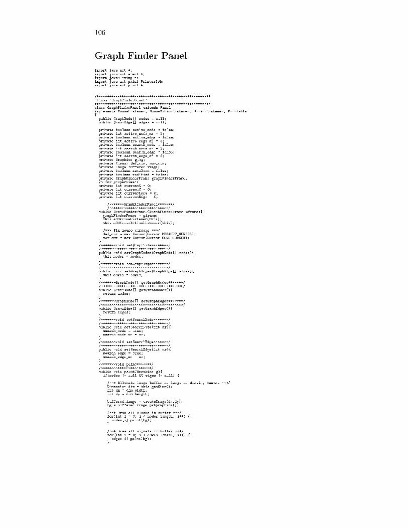
106
Graph Finder Panel
import java.awt.*;import java.awt.event.*;import javax.swing.*;import java.awt.print.PrinterJob;import java.awt.print.*;
/******************************************************Class "GraphFinderPanel"
******************************************************/class GraphFinderPanel extends Panelimplements MouseListener, MouseMotionListener, ActionListener, Printable{
public GraphNode[] nodes = null;public GraphEdge[] edges = null;
private boolean active_node = false;private int active_node_nr = 0;private boolean active_edge = false;private int active_edge_nr = 0;private boolean search_node = false;private int search_node_nr = 0;private boolean search_edge = false;private int search_edge_nr = 0;private Graphics g,bg;private Cursor def_cur, mov_cur;private Image buffered_image;private boolean metaDown = false;private boolean modified = false;private GraphFinderFrame graphFinderFrame;/* for properties*/private int currentX = 0;private int currentY = 0;private int currentNode = 0;private int currentEdge = 0;
/*******GraphFinderPanel*******//****************************/
public GraphFinderPanel(GraphFinderFrame pframe){graphFinderFrame = pframe;this.addMouseListener(this);this.addMouseMotionListener(this);
/*** Fix mouse cursors ***/def_cur = new Cursor(Cursor.DEFAULT_CURSOR);mov_cur = new Cursor(Cursor.MOVE_CURSOR);
}/*******void setGraphNodes*******//********************************/public void setGraphNodes(GraphNode[] nodes){
this.nodes = nodes;}/*******void setGraphEdges*******//********************************/public void setGraphEdges(GraphEdge[] edges){
this.edges = edges;}/*******GraphNode[] getGraphNodes*******//***************************************/public GraphNode[] getGraphNodes(){
return nodes;}/*******GraphEdge[] getGraphEdges*******//***************************************/public GraphEdge[] getGraphEdges(){
return edges;}/*******void setSearchNode*******//********************************/public void setSearchNode(int nr){
search_node = true;search_node_nr = nr;
}/*******void setSearchEdge*******//********************************/public void setSearchEdge(int nr){
search_edge = true;search_edge_nr = nr;
}/*******void paint*******//************************/public void paint(Graphics g){
if(nodes != null && edges != null) {
/*** Allocate image buffer as large as drawing canvas ***/Dimension dim = this.getSize();int dx = dim.width;int dy = dim.height;
buffered_image = createImage(dx,dy);bg = buffered_image.getGraphics();
/*** Draw all blocks in buffer ***/for(int i = 0; i < nodes.length; i++) {
nodes[i].paint(bg);}
/*** Draw all signals in buffer ***/for(int i = 0; i < edges.length; i++) {
edges[i].paint(bg);}
107
/*** Copy buffer on screen ***/g.drawImage(buffered_image,0,0,null);// bg.dispose();// buffered_image.flush();
}}/*******void mouseReleased*******//********************************/public void mouseReleased(MouseEvent e) {
if(nodes != null && edges != null) {if(modified){
graphFinderFrame.setModified();modified = false;
}
for(int i=0; i<nodes.length; i++) {if(metaDown == true && nodes[i].isActive()){
popupMenu(e);metaDown = false;
}nodes[i].setNonActive();
}for(int i=0; i<edges.length; i++) {
if(metaDown == true && edges[i].isActive()){popupMenu(e);metaDown = false;
}edges[i].setNonActive();
}active_node = false;active_node_nr = 0;active_edge = false;active_edge_nr = 0;this.setCursor(def_cur);g = getGraphics();this.paint(g);
}}/*******void mousePressed*******//*******************************/public void mousePressed(MouseEvent e) {
int mx = e.getX();int my = e.getY();int sx,sy;
if(nodes != null && edges != null) {if(e.isMetaDown()){
metaDown = true;}if(search_node){
nodes[search_node_nr].setSearch(false);search_node = false;search_node_nr = 0;
}if(search_edge){
edges[search_edge_nr].setSearch(false);search_edge = false;search_edge_nr = 0;
}
for(int i=0; i<nodes.length && active_node==false; i++) {sx = nodes[i].getX();sy = nodes[i].getY();if(mx>=(sx-15) && mx<=(sx+15) && my>=(sy-15) && my<=(sy+15)) {
nodes[i].setActive();active_node = true;active_node_nr = i;this.setCursor(mov_cur);
}}if(active_node == false) {
for(int i=0; i<edges.length && active_edge==false; i++) {sx = edges[i].getX();sy = edges[i].getY();if(mx>=(sx-3) && mx<=(sx+3) && my>=(sy-3) && my<=(sy+3)) {
edges[i].setActive();active_edge = true;active_edge_nr = i;this.setCursor(mov_cur);
}}
}g = getGraphics();this.paint(g);
}}/*******void mouseDragged*******//*******************************/public void mouseDragged(MouseEvent e) {
if(nodes != null && edges != null) {Insets insets = getInsets();int containerWidth = getSize().width - insets.left - insets.right-15;int containerHeight = getSize().height - insets.top - insets.bottom-15;
if(e.getX()>=15 && e.getY()>=15&& e.getX()<=containerWidth && e.getY()<=containerHeight){
if(active_node)nodes[active_node_nr].setXY(e.getX(),e.getY());
if(active_edge)edges[active_edge_nr].setXY(e.getX(),e.getY());
if(active_node || active_edge)modified = true;
g = getGraphics();
108
this.paint(g);}
}}/*******void mouseClicked*******//*******************************/public void mouseClicked(MouseEvent e) {
int mx = e.getX();int my = e.getY();int sx,sy;
if(nodes != null && edges != null){if(e.getClickCount() >= 2){
boolean found = false;
for(int i=0; i<nodes.length && found == false; i++) {sx = nodes[i].getX();sy = nodes[i].getY();if(mx>=(sx-15) && mx<=(sx+15) && my>=(sy-15) && my<=(sy+15)){
found = true;if(nodes[i].getNodeName() == null){
GraphFinderFrame frame =new GraphFinderFrame(nodes[i].getName() + ".txt",
graphFinderFrame.getDirName());frame.show();
}}
}}
}}/*******void mouseEntered*******//*******************************/public void mouseEntered(MouseEvent e) {;}/*******void mouseExited*******//******************************/public void mouseExited(MouseEvent e) {;}/*******void mouseMoved*******//*****************************/public void mouseMoved(MouseEvent e) {;}/*******void actionPerformed*******//**********************************/public void actionPerformed(ActionEvent e){
String arg = e.getActionCommand();
if(arg.equals("View Code Items")){GraphFinderFrame frame =
new GraphFinderFrame(nodes[currentNode].getName() + ".txt",graphFinderFrame.getDirName());
frame.show();}else if(arg.equals("Node Properties")||
arg.equals("Edge Properties")){
final JFrame frame = new JFrame("Properties");frame.addWindowListener(new WindowAdapter() {
public void windowClosing(WindowEvent e){frame.dispose();
}});if( arg.equals("Node Properties"))
frame.getContentPane().add(new ObjectProperties(nodes[currentNode]),BorderLayout.CENTER);
elseframe.getContentPane().add(new ObjectProperties(edges[currentEdge]),
BorderLayout.CENTER);frame.setBounds(currentX, currentY, 240, 120);frame.setVisible(true);
}}/*******void popupMenu*******//****************************/private void popupMenu(MouseEvent e){
MenyMaker menyM = new MenyMaker();PopupMenu popup = new PopupMenu();
if(active_node && nodes[active_node_nr].getNodeName() == null){/* node active */currentNode = active_node_nr;menyM.makeMenu(popup, new Object[]{
"View Code Items",null,"Node Properties"}, this);
}else if(active_node && nodes[active_node_nr].getNodeName() != null){
/* item active */currentNode = active_node_nr;menyM.makeMenu(popup,
new Object[]{"Node Properties"
}, this);}else if(active_edge){
/* edge active*/currentEdge = active_edge_nr;menyM.makeMenu(popup, new Object[]{
"Edge Properties"}, this);
}add(popup);popup.show(e.getComponent(), e.getX(), e.getY());Point p = getLocationOnScreen();currentX = p.x + e.getX();currentY = p.y + e.getY();
109
}/*******void printFile*******//****************************/public void printFile(){
PrinterJob printJob = PrinterJob.getPrinterJob();printJob.setPrintable(this);if (printJob.printDialog()) {
try {printJob.print();
}catch (Exception ex) {
ex.printStackTrace();}
}}/*******int print*******//***********************/public int print(Graphics g, PageFormat pf, int pi) throws PrinterException {
if (pi >= 1) {return Printable.NO_SUCH_PAGE;
}paint(g);return Printable.PAGE_EXISTS;
}}
110
Input File
import java.awt.*;import java.awt.event.*;import javax.swing.*;import java.util.*;import java.io.*;
/******************************************************Class "InputFile"*******************************************************/class InputFile{
private String fileName;private String dirName;private Vector nodes = null;private Vector edges = null;private GraphFinderPanel graphFinderPanel;private int defaultWindowSize = 500;
/*******InputFile*******//***********************/public InputFile(String fileName, String dirName, GraphFinderPanel graphFinderPanel){this.fileName = fileName;this.dirName = dirName;this.graphFinderPanel = graphFinderPanel;nodes = new Vector();edges = new Vector();
}/*******readFile*******//**********************/public boolean readFile(){
try{BufferedReader in = new BufferedReader(new
FileReader(dirName + fileName));
readData(in);in.close();
}catch(IOException e){
JOptionPane.showMessageDialog(graphFinderPanel,"Can't open file: " + dirName + fileName,"File warning",JOptionPane.WARNING_MESSAGE);
return false;}try{
int length = fileName.length();String fName = fileName.substring(0, length-4) + "_coord.txt";
BufferedReader in = new BufferedReader(newFileReader(dirName + fName));
readData(in);in.close();
}catch(IOException e){
/* no file with coordinates found *//* set default coordinates values for nodes */GraphNode[] node = new GraphNode[nodes.size()];nodes.copyInto(node);
if(node.length > 35)setCoordinatesRandom(node);
elsesetCoordinatesCircle(node);
/* set default coordinates values for nodes */GraphEdge[] edge = new GraphEdge[edges.size()];edges.copyInto(edge);
/* This loop is done to calculate proper knee coordinates */for (int i = 0; i < edge.length; i++){
GraphNode from = edge[i].getFromNode();
111
GraphNode to = edge[i].getToNode();int kx = (from.getX() + to.getX())/2;int ky = (from.getY() + to.getY())/2;
edge[i].setXY(kx,ky);}
}
return true;}/*******void readData*******//***************************/private void readData(BufferedReader in) throws IOException{
String line;String s = "";
while((line = in.readLine()) != null){
StringTokenizer t = new StringTokenizer(line, "., \t\n\r");
while(t.hasMoreTokens()){s = t.nextToken();
if(s.equals("#")){t = new StringTokenizer(line, "\n\r");s = t.nextToken();
}else if(s.equals("bl")){GraphNode node = new GraphNode(t.nextToken());nodes.addElement(node);
}else if(s.equals("bs")){
GraphEdge edge = new GraphEdge();edge.setFromNode(findNode(t.nextToken()));edge.setToNode(findNode(t.nextToken()));edge.setName(t.nextToken());edge.setType(t.nextToken());edge.setTime(Integer.parseInt(t.nextToken()));edges.addElement(edge);
}else if(s.equals("ci")){
String nodeName = t.nextToken();String name = t.nextToken();GraphNode node = new GraphNode(name, nodeName);nodes.addElement(node);
}else if(s.equals("is")){
GraphEdge edge = new GraphEdge();edge.setNodeName(t.nextToken());edge.setFromNode(findNode(t.nextToken()));edge.setToNode(findNode(t.nextToken()));edge.setName(t.nextToken());edge.setType(t.nextToken());edge.setTime(Integer.parseInt(t.nextToken()));edges.addElement(edge);
}else if(s.equals("nc")){
findNode(t.nextToken()).setXY(Integer.parseInt(t.nextToken()),Integer.parseInt(t.nextToken()));
}
else if(s.equals("ec")){findEdge(t.nextToken()).setXY(Integer.parseInt(t.nextToken()),
Integer.parseInt(t.nextToken()));}else{/* can not read the file foramt,
therefore throws an exception */throw new IOException();
}}
}}/*******GraphNode findNode*******//********************************/private GraphNode findNode(String nodeName){
for(int i=0; i < nodes.size(); i++){GraphNode node = (GraphNode)nodes.elementAt(i);
112
if(nodeName.equals(node.getName()))return node;
}return null;
}/*******GraphEdge findEdge*******//********************************/private GraphEdge findEdge(String edgeName){
for(int i=0; i < edges.size(); i++){GraphEdge edge = (GraphEdge)edges.elementAt(i);
if(edgeName.equals(edge.getName()))return edge;
}return null;
}/*******GraphNode*******//***********************/public GraphNode[] getGraphNodes(){
GraphNode[] node = new GraphNode[nodes.size()];nodes.copyInto(node);nodes = null;
return node;}/*******GraphEdge*******//***********************/public GraphEdge[] getGraphEdges(){
GraphEdge[] edge = new GraphEdge[edges.size()];edges.copyInto(edge);edges = null;
return edge;}/*******void setCoordinatesRandom*******//***************************************/public void setCoordinatesRandom(GraphNode[] nodes){
int x;int y;
Insets insets = graphFinderPanel.getInsets();int containerWidth = graphFinderPanel.getSize().width - insets.left - insets.right - 75;int containerHeight = graphFinderPanel.getSize().height - insets.top - insets.bottom - 75;
if(containerWidth == 0 && containerHeight == 0){containerWidth = defaultWindowSize;containerHeight = defaultWindowSize;
}System.out.println(containerWidth);System.out.println(containerHeight);
for(int i=0; i<nodes.length; i++){
boolean checked = false;do{x = (int)(Math.random()*containerWidth) + 20;y = (int)(Math.random()*containerHeight) + 20;
boolean found = false;for(int j=0; j<i && found == false; j++){
int x1 = nodes[j].getX() - 59;int y1 = nodes[j].getY() - 59;
Rectangle r = new Rectangle(x1,y1,118,118);if(r.contains(x,y))found = true;
}if(found == false){
checked = true;nodes[i].setXY(x,y);
}}while(checked == false);
}}/*******void setCoordinatesCircle*******/
113
/***************************************/public void setCoordinatesCircle(GraphNode[] nodes){
Insets insets = graphFinderPanel.getInsets();int containerWidth = graphFinderPanel.getSize().width - insets.left - insets.right;int containerHeight = graphFinderPanel.getSize().height - insets.top - insets.bottom;
if(containerWidth == 0 && containerHeight == 0){containerWidth = defaultWindowSize;containerHeight = defaultWindowSize;
}
int n = nodes.length;int size;if(n > 15)
size = 50;else
size = 200;
int xradius = (containerWidth - size)/ 2;int yradius = (containerHeight - size)/ 2;
int xcenter = insets.left + containerWidth / 2;int ycenter = insets.top + containerHeight / 2;
for (int i = 0; i < n; i++){double angle = 2 * Math.PI * i / n;int x = xcenter + (int)(Math.cos(angle) * xradius);int y = ycenter + (int)(Math.sin(angle) * yradius);
nodes[i].setXY(x,y);}
}/*******boolean writeToFile*******//*********************************/public boolean writeToFile(GraphNode[] nodes, GraphEdge[] edges){
try{PrintWriter out = new PrintWriter(new FileWriter(dirName + fileName));writeData(out,nodes,edges);out.close();
}catch(Exception e){
return false;}try{
int length = fileName.length();String fName = fileName.substring(0, length-4) + "_coord.txt";PrintWriter out = new PrintWriter(new FileWriter(dirName + fName));saveCoordinates(out,nodes,edges);out.close();
}catch(Exception e){ /* coordinates could not be saved */ }
return true;}/*******void writeData*******//****************************/public void writeData(PrintWriter out,GraphNode[] nodes, GraphEdge[] edges)
throws IOException{boolean codeItems = true;/* write default text for nodes*/if(nodes[0].getNodeName() == null){
codeItems = false;}
if(codeItems == false){out.println("#");out.println("# Define all blocks");out.println("#");out.println("# bl.[name].");out.println("#");
}else{
out.println("#");out.println("# Define all code items for a block");out.println("#");out.println("# ci[block name].[name].");out.println("#");
114
}for(int i=0; i<nodes.length; i++){if(codeItems == false){
out.println("bl." +nodes[i].getName() + ".");
}else{
out.println("ci." +nodes[i].getNodeName() + "." +nodes[i].getName() + ".");
}}/* write default text for edges*/if(codeItems == false){out.println("#");out.println("# Define signals to all blocks");out.println("#");out.println("# bs.[from block].[to block].[signal name].[type].[time].");out.println("#");
}else{out.println("#");out.println("# Define signals to all code items");out.println("#");out.println("# is.[block name].[from item].[to item].[signal name].[type].[time].");out.println("#");
}for(int i=0; i<edges.length; i++){if(codeItems == false){
out.println("bs." +edges[i].getFromNode().getName() + "." +edges[i].getToNode().getName() + "." +edges[i].getName() + "." +edges[i].getType() + "." +edges[i].getTime() + ".");
}else{
out.println("is." +edges[i].getNodeName() + "." +edges[i].getFromNode().getName() + "." +edges[i].getToNode().getName() + "." +edges[i].getName() + "." +edges[i].getType() + "." +edges[i].getTime() + ".");
}}
}/*******void saveCoordinates*******//**********************************/private void saveCoordinates(PrintWriter out,GraphNode[] nodes, GraphEdge[] edges)
throws IOException{out.println("#");out.println("# Define all coordinates for nodes");out.println("#");out.println("# nc.[name].[x coordinate].[y coordinate].");out.println("#");
for(int i=0; i<nodes.length; i++){out.println("nc." +
nodes[i].getName() + "." +nodes[i].getX() + "." +nodes[i].getY() + ".");
}
out.println("#");out.println("# Define all coordinates for edges");out.println("#");out.println("# ec.[signal name].[x coordinate].[y coordinate].");out.println("#");
for(int i=0; i<edges.length; i++){out.println("ec." +
edges[i].getName() + "." +edges[i].getX() + "." +edges[i].getY() + ".");
}}

115
}
116
Graph Object
import java.awt.*;import java.awt.event.*;
/******************************************************Class "GraphObject"*******************************************************/
class GraphObject{
int x = 0;int y = 0;int time = 0;
String nodeName = null;String name;String info;
boolean showtime = true;boolean showname = true;boolean active = false;boolean search = false;
/*******GraphObject*******//*************************/public GraphObject() {}/*******GraphObject*******//*************************/public GraphObject(String inName) {
name = inName;}/*******GraphObject*******//*************************/public GraphObject(String inName, String inNodeName) {
name = inName;nodeName = inNodeName;
}/*******String getNodeName*******//********************************/public String getNodeName(){
return nodeName;}/*******void setNodeName*******//******************************/public void setNodeName(String inNodeName){
nodeName = inNodeName;}/*******void setSearch*******//****************************/public void setSearch(boolean b){
search = b;}/*******int getX*******//**********************/public int getX() {
return x;}/*******int getY*******//**********************/public int getY() {
return y;}/*******void setXY*******//************************/public void setXY(int a, int b) {
x = a;y = b;
}/*******String getName*******//****************************/public String getName() {
return name;}/*******void setName*******//**************************/
117
public void setName(String a) {name = a;
}/*******String getInfo*******//****************************/public String getInfo() {
return info;}/*******void setInfo*******//*************************/public void setInfo(String a) {
info = a;}/*******int getTime*******//*************************/public int getTime() {
return time;}/*******void setTime*******//**************************/public void setTime(int a) {
time = a;}/*******void toggleShowTime*******//*********************************/public void toggleShowTime() {
if(showtime==true)showtime=false;
elseshowtime=true;
}/*******void toggleShowName*******//*********************************/public void toggleShowName() {
if(showname==true)showname=false;
elseshowname=true;
}/*******void setActive*******//****************************/public void setActive() {
active = true;}/*******void setNonActive*******//*******************************/public void setNonActive() {
active = false;}/*******boolean isActive*******//******************************/public boolean isActive(){
return active;}/*******void paint*******//************************/public void paint(Graphics gr) {}
}
/******************************************************Class "GraphNode"
*******************************************************/class GraphNode extends GraphObject{/*******GraphNode*******//***********************/public GraphNode(String name){
super(name);}/*******GraphNode*******//***********************/public GraphNode(String name, String nodeName){
super(name, nodeName);}/*******void paint*******//*************************/
118
public void paint(Graphics gr) {gr.setColor(Color.black);gr.drawRect(x-15,y-15,30,30);
if (active) {gr.setColor(Color.red);
}else if(search){
gr.setColor(Color.yellow);}else {
gr.setColor(Color.cyan);}
gr.fillRect(x-14,y-14,29,29);if(showname) {
gr.setColor(Color.blue);gr.drawString(name,x,y);
}}
}
/******************************************************Class "GraphEdge"*******************************************************/class GraphEdge extends GraphObject{
GraphNode fromNode = null;GraphNode toNode = null;String type = "";
boolean showDir = true;boolean showBuf = true;
/*******GraphEdge*******//***********************/
public GraphEdge(){}/*******void setFromNode*******//******************************/public void setFromNode(GraphNode node) {
fromNode = node;}/*******void setToNode*******//****************************/public void setToNode(GraphNode node) {
toNode = node;}/*******void setType*******//**************************/public void setType(String type){
this.type = type;}/*******GraphNode getFromNode*******//***********************************/public GraphNode getFromNode() {
return fromNode;}/*******GraphNode getToNode*******//*********************************/public GraphNode getToNode() {
return toNode;}/*******String getType*******//****************************/public String getType(){
return type;}/*******void toggleShowDir*******//********************************/public void toggleShowDir(){
if(showDir==true)showDir=false;
elseshowDir=true;
}/*******void toggleShowBuf*******/
119
/********************************/public void toggleShowBuf(){
if(showBuf==true)showBuf=false;
elseshowBuf=true;
}/*******void paint*******//************************/public void paint(Graphics gr) {
int x1,y1,x2,y2,tx,ty1,ty2,nx,ny1,ny2;double c1,c2;String test;
x1 = fromNode.getX();y1 = fromNode.getY();x2 = toNode.getX();y2 = toNode.getY();tx = (x-x1)/2;ty1 = (y-y1)/2;ty2 = (y-y1)/2;nx = (x2-x)/3;ny1 = (y2-y)/3;ny2 = (y2-y)/3;
/* Draw lines */gr.setColor(Color.black);
if(y < y2) {gr.drawLine(x1,y1,x,y);gr.drawLine(x,y,x2,y2-25);gr.drawLine(x2,y2-15,x2,y2-25);gr.drawLine(x2-5,y2-25,x2,y2-15);gr.drawLine(x2+5,y2-25,x2,y2-15);
}else {
gr.drawLine(x1,y1,x,y);gr.drawLine(x,y,x2,y2+25);gr.drawLine(x2,y2+15,x2,y2+25);gr.drawLine(x2-5,y2+25,x2,y2+15);gr.drawLine(x2+5,y2+25,x2,y2+15);
}
/* Draw knee */if (active) {
gr.setColor(Color.red);}else if(search){
gr.setColor(Color.yellow);}else {
gr.setColor(Color.black);}gr.fillRect(x-3,y-3,7,7);
/* Draw time stamp */if(showtime==true) {
test = Integer.toString(time);if(y1 < y2) {
gr.setColor(Color.red);gr.drawString(test,tx+x1-4,ty1+y1+5);
} else {gr.setColor(Color.red);gr.drawString(test,tx+x1-4,ty2+y1+5);
}}/* Draw name stamp */if(showname==true) {
if((showDir ==true && type.equals("dir")) ||(showBuf==true && type.equals("buf"))){
if(y1 < y2) {gr.setColor(Color.red);gr.drawString(name,nx+x-4,ny1+y+5);
} else {gr.setColor(Color.red);gr.drawString(name,nx+x-4,ny2+y+5);
}

120
}}
}}
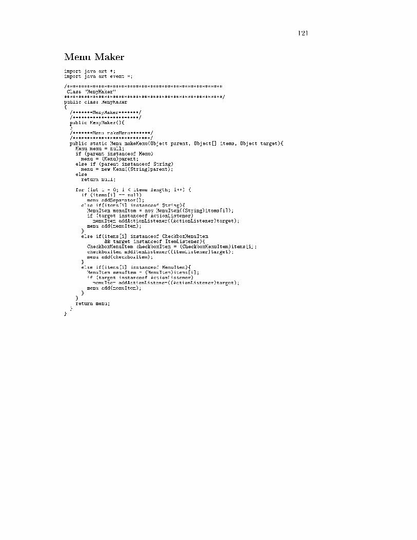
121
Menu Maker
import java.awt.*;import java.awt.event.*;
/******************************************************Class "MenyMaker"*******************************************************/public class MenyMaker{/*******MenyMaker*******//***********************/public MenyMaker(){}/*******Menu makeMenu*******//***************************/public static Menu makeMenu(Object parent, Object[] items, Object target){
Menu menu = null;if (parent instanceof Menu)
menu = (Menu)parent;else if (parent instanceof String)
menu = new Menu((String)parent);else
return null;
for (int i = 0; i < items.length; i++) {if (items[i] == null)
menu.addSeparator();else if(items[i] instanceof String){
MenuItem menuItem = new MenuItem((String)items[i]);if (target instanceof ActionListener)menuItem.addActionListener((ActionListener)target);
menu.add(menuItem);}else if(items[i] instanceof CheckboxMenuItem
&& target instanceof ItemListener){CheckboxMenuItem checkboxItem = (CheckboxMenuItem)items[i];checkboxItem.addItemListener((ItemListener)target);menu.add(checkboxItem);
}else if(items[i] instanceof MenuItem){
MenuItem menuItem = (MenuItem)items[i];if (target instanceof ActionListener)menuItem.addActionListener((ActionListener)target);
menu.add(menuItem);}
}return menu;
}}
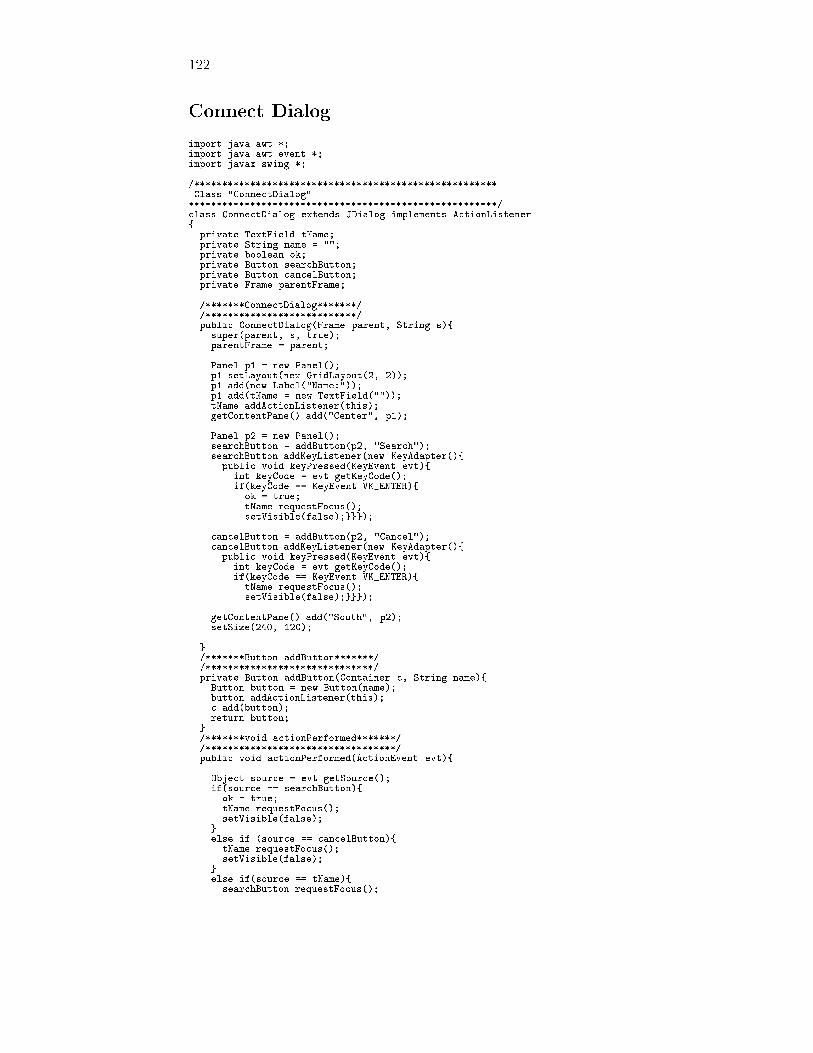
122
Connect Dialog
import java.awt.*;import java.awt.event.*;import javax.swing.*;
/******************************************************Class "ConnectDialog"*******************************************************/class ConnectDialog extends JDialog implements ActionListener{
private TextField tName;private String name = "";private boolean ok;private Button searchButton;private Button cancelButton;private Frame parentFrame;
/*******ConnectDialog*******//***************************/public ConnectDialog(Frame parent, String s){
super(parent, s, true);parentFrame = parent;
Panel p1 = new Panel();p1.setLayout(new GridLayout(2, 2));p1.add(new Label("Name:"));p1.add(tName = new TextField(""));tName.addActionListener(this);getContentPane().add("Center", p1);
Panel p2 = new Panel();searchButton = addButton(p2, "Search");searchButton.addKeyListener(new KeyAdapter(){
public void keyPressed(KeyEvent evt){int keyCode = evt.getKeyCode();if(keyCode == KeyEvent.VK_ENTER){
ok = true;tName.requestFocus();setVisible(false);}}});
cancelButton = addButton(p2, "Cancel");cancelButton.addKeyListener(new KeyAdapter(){
public void keyPressed(KeyEvent evt){int keyCode = evt.getKeyCode();if(keyCode == KeyEvent.VK_ENTER){
tName.requestFocus();setVisible(false);}}});
getContentPane().add("South", p2);setSize(240, 120);
}/*******Button addButton*******//******************************/private Button addButton(Container c, String name){
Button button = new Button(name);button.addActionListener(this);c.add(button);return button;
}/*******void actionPerformed*******//**********************************/public void actionPerformed(ActionEvent evt){
Object source = evt.getSource();if(source == searchButton){
ok = true;tName.requestFocus();setVisible(false);
}else if (source == cancelButton){
tName.requestFocus();setVisible(false);
}else if(source == tName){
searchButton.requestFocus();
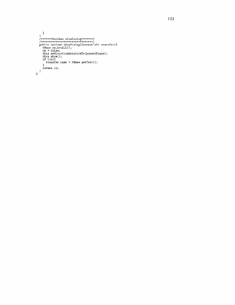
123
}}/*******boolean showDialog*******//********************************/public boolean showDialog(ConnectInfo transfer){
tName.selectAll();ok = false;this.setLocationRelativeTo(parentFrame);this.show();if (ok){
transfer.name = tName.getText();}return ok;
}}
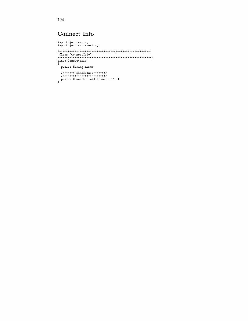
124
Connect Info
import java.awt.*;import java.awt.event.*;
/******************************************************Class "ConnectInfo"*******************************************************/class ConnectInfo{
public String name;
/*******ConnectInfo*******//*************************/public ConnectInfo() {name = ""; }
}
125
Object Properties
import javax.swing.JTabbedPane;import javax.swing.ImageIcon;import javax.swing.JLabel;import javax.swing.JPanel;import javax.swing.JFrame;import javax.swing.*;
import java.awt.*;import java.awt.event.*;
/******************************************************Class "ObjectProperties"*******************************************************/public class ObjectProperties extends JPanel{/*******ObjectProperties*******//******************************/public ObjectProperties(GraphNode node) {
ImageIcon icon = new ImageIcon("images/middle.gif");JTabbedPane tabbedPane = new JTabbedPane();
Box b;b = Box.createVerticalBox();
b.add(new JLabel(" Name: " + node.getName()));if(node.getNodeName() != null)
b.add(new JLabel(" Node name: " + node.getNodeName()));
tabbedPane.addTab("Generally", icon, b, "Information about node");tabbedPane.setSelectedIndex(0);
//Add the tabbed pane to this panel.setLayout(new GridLayout(1, 1));add(tabbedPane);
}/*******ObjectProperties*******//******************************/public ObjectProperties(GraphEdge edge) {
ImageIcon icon = new ImageIcon("images/middle.gif");JTabbedPane tabbedPane = new JTabbedPane();
Box b1;b1 = Box.createVerticalBox();b1.add(new JLabel(" Name: " + edge.getName()));if(edge.getNodeName() != null)b1.add(new JLabel(" Block name: " + edge.getNodeName()));
if(edge.getType().equals("dir"))b1.add(new JLabel(" Type: direct signal"));
else if(edge.getType().equals("buf"))b1.add(new JLabel(" Type: buffered signal"));
//b1.add(new JLabel(" Type: " + edge.getType()));tabbedPane.addTab("Generally", icon, b1, "Information about edge");tabbedPane.setSelectedIndex(0);
Box b2;b2 = Box.createVerticalBox();b2.add(new JLabel(" Time: "+ edge.getTime()));b2.add(new JLabel(" Total time: " + "?"));tabbedPane.addTab("Time", icon, b2, "Time information");
//Add the tabbed pane to this panel.setLayout(new GridLayout(1, 1));add(tabbedPane);
}}


![C OMMUNIC A TIONS2005/04/04 · C OMMUNIC A TIONS K OMUNIKÁCIE / COMMUNICATIONS 2/2004 51. Introduction The HSDPA concept (High Speed Downlink Packet Access, e.g., [1], [2]) of UMTS](https://img.pdfslide.net/doc/110x75/5f9735d6b26a6e7d453e68bc/c-ommunic-a-20050404-c-ommunic-a-tions-k-omunikcie-communications-22004.jpg)