Master Thesis

Analysis tools for multiexponentialenergy decay curves in room acoustics

conducted at theSignal Processing and Speech Communications Laboratory

Graz University of Technology, Austria

byFlorian Muralter, 00873103

Supervisor:Dipl.-Ing. Jamilla Balint

Assessor/Examiner:Ao.Univ.-Prof. Dipl.-Ing. Dr. techn. Gerhard Graber

June, 2018

Abstract:Energy decay curves in roomacoustics can exhibit a multiexponential nature. Multiple slopedenergy decay curves do not exclusively exist in coupled volume spaces, where they are used toadapt the acoustic behaviour (e.g., in concert halls), but also in reverberation chambers. Oncea curved decay is present, the commonly used method of fitting a linear regression to obtainthe reverberation time becomes questionable. This work investigates three state-of-the-art al-gorithms to extract decay times from a given energy decay curve (EDC). The first is a revisedversion of the variable projection algorithm (VARPRO). The second and third program are bothbased on the assumption that a decay time distribution can be computed from the given EDC bycomputing the inverse Laplace transform. The Regularized Inverse Laplace Transform algorithm(RILT) uses a nonlinear least squares fitting algorithm to extract the intensities for a specifieddecay time grid with a regularisation based on the principle of parsimony. The obtained inten-sities as a function of the decay times can then be regarded as a decay time distribution. TheMaximum Entropy Decay time Distribution program (MEDD) computes a decay time distribu-tion using a quantified maximum entropy method. Measurements from a reverberation chamberare analysed, decay times and decay time distributions are estimated using the proposed meth-ods. Furthermore, the obtained results are used to define the single sloped frequency range ina reverberation chamber, such that rough bounds for the validity of the commonly used linearregression method can be given.

Zusammenfassung:Abklingkurven in der Raumakustik konnen ein multiexponentielles Verhalten aufweisen. Mehrereunterschiedliche Steigungen konnen nicht nur in Abklingkurven von gekoppelten Raumen ge-funden werden sondern auch in Hallraumen. Sobald eine in der logarithmischen Darstellunggekrummte Abklingkurve zu erkennen ist verliert die Methode zur Berechnung der Nachhallzeitmittels einer linearen Regression ihre Richtigkeit. Diese Arbeit beschaftigt sich mit der Entwick-lung und Erprobung dreier unterschiedlicher state-of-the-art Algorithmen zur Bestimmung derAbklingzeiten einer gegebenen Abklingkurve. Als erste Methode wird eine uberarbeitete Ver-sion des Variable Projection Algorithm (VARPRO) untersucht. Die zwei weiteren Programmebasieren auf der Hypothese, dass sich die Verteilung der Abklingzeiten aus der Abklingkurve mit-tels einer inversen Laplace Transformation berechnen lasst. Das Programm Regularized InverseLaplace Transform (RILT) verwendet hierfur einen nichtlinearen Least Squares Fitting Algorith-mus dessen Regularisierungsterm auf dem Prinzip der Sparsamkeit beruht. Im Programm Max-imum Entropy Decay time Distribution (MEDD) wird die Verteilung der Abklingzeiten mittelseiner Quantified Maximum Entropy Method berechnet. Messungen aus einem Hallraum werdenanalysiert, Abklingzeiten und Verteilungen der Abklingzeiten mittels der angesprochenen Meth-oden berechnet. Die resultierenden Verteilungen werden dazu verwendet einen Frequenzbereichzu definieren, in welchem sich ein im logarithmischen Maß linearer Abklingvorgang einstellt.Dieser Bereich ermoglicht auch die Angabe von Grenzen fur die Richtigkeit der ursprunglichenBerechnung der Nachhallzeit mittels einer linearen Regression in Hallraumen.

Statutory Declaration

I declare that I have authored this thesis independently, that I have not used other thanthe declared sources/resources and that I have explicitly marked all material which has beenquoted either literally or by content from the sources used. The text document uploaded toTUGRAZonline is identical to the present master’s thesis.

date (signature)

Contents

1 Introduction 11.1 Introduction and Motivation . . . . . . . . . . . . . . . . . . . . . . . . . . . . . . 11.2 Summary of Chapters . . . . . . . . . . . . . . . . . . . . . . . . . . . . . . . . . 3

2 Theory 42.1 Sound in Enclosures . . . . . . . . . . . . . . . . . . . . . . . . . . . . . . . . . . 4

2.1.1 Wave Based Roomacoustics . . . . . . . . . . . . . . . . . . . . . . . . . . 42.1.2 Statistical Roomacoustics . . . . . . . . . . . . . . . . . . . . . . . . . . . 82.1.3 Calculation and Measurement of the Reverberation Time . . . . . . . . . 9

2.2 The Double Sloped Effect [DSE] . . . . . . . . . . . . . . . . . . . . . . . . . . . 112.2.1 Coupled Volume Spaces . . . . . . . . . . . . . . . . . . . . . . . . . . . . 112.2.2 Reverberation Chamber . . . . . . . . . . . . . . . . . . . . . . . . . . . . 12

2.3 The Decay rate Distribution . . . . . . . . . . . . . . . . . . . . . . . . . . . . . . 142.4 Noise treatment . . . . . . . . . . . . . . . . . . . . . . . . . . . . . . . . . . . . . 16

3 Methodologies 183.1 VARPRO - Variable Projection Algorithm . . . . . . . . . . . . . . . . . . . . . . 183.2 RILT - Regularized Inverse Laplace Transform . . . . . . . . . . . . . . . . . . . 203.3 MELT - Maximum Entropy Lifetime Analysis . . . . . . . . . . . . . . . . . . . . 23

4 MEDD - Maximum Entropy Decay Time Distribution 274.1 Structure . . . . . . . . . . . . . . . . . . . . . . . . . . . . . . . . . . . . . . . . 274.2 Subprograms . . . . . . . . . . . . . . . . . . . . . . . . . . . . . . . . . . . . . . 28

5 Measurement Conditions 325.1 Measurement Setup . . . . . . . . . . . . . . . . . . . . . . . . . . . . . . . . . . 325.2 Diffusors and Absorbers . . . . . . . . . . . . . . . . . . . . . . . . . . . . . . . . 335.3 Calculation of the EDC . . . . . . . . . . . . . . . . . . . . . . . . . . . . . . . . 34

6 Test Cases 356.1 VARPRO . . . . . . . . . . . . . . . . . . . . . . . . . . . . . . . . . . . . . . . . 35

6.1.1 Single slope estimation . . . . . . . . . . . . . . . . . . . . . . . . . . . . . 356.1.2 Multiple slope estimation . . . . . . . . . . . . . . . . . . . . . . . . . . . 376.1.3 Results . . . . . . . . . . . . . . . . . . . . . . . . . . . . . . . . . . . . . 39

6.2 RILT . . . . . . . . . . . . . . . . . . . . . . . . . . . . . . . . . . . . . . . . . . . 406.2.1 Results . . . . . . . . . . . . . . . . . . . . . . . . . . . . . . . . . . . . . 42

6.3 MEDD . . . . . . . . . . . . . . . . . . . . . . . . . . . . . . . . . . . . . . . . . . 436.3.1 Evaluation of extracted decay times . . . . . . . . . . . . . . . . . . . . . 436.3.2 Variation of user specified variables . . . . . . . . . . . . . . . . . . . . . . 446.3.3 Results . . . . . . . . . . . . . . . . . . . . . . . . . . . . . . . . . . . . . 45

6.4 MEDD vs. RILT . . . . . . . . . . . . . . . . . . . . . . . . . . . . . . . . . . . . 466.4.1 Single sloped EDCs . . . . . . . . . . . . . . . . . . . . . . . . . . . . . . 466.4.2 Multiple sloped EDCs . . . . . . . . . . . . . . . . . . . . . . . . . . . . . 47

7 Results 507.1 The 25 Hz band . . . . . . . . . . . . . . . . . . . . . . . . . . . . . . . . . . . . . 507.2 Frequency range of single sloped behaviour . . . . . . . . . . . . . . . . . . . . . 54

7.2.1 Octave band vs. 13 -Octave band . . . . . . . . . . . . . . . . . . . . . . . . 56

7.2.2 Number of Absorbers . . . . . . . . . . . . . . . . . . . . . . . . . . . . . 587.2.3 Number of Diffusors . . . . . . . . . . . . . . . . . . . . . . . . . . . . . . 61

Graz, June 12, 2018 – iii –

8 Conclusion and Outlook 64

A Appendix 66List of Symbols and Abbreviatiosn . . . . . . . . . . . . . . . . . . . . . . . . . . . . . 67Data used for Figures . . . . . . . . . . . . . . . . . . . . . . . . . . . . . . . . . . . . 68List of Figures . . . . . . . . . . . . . . . . . . . . . . . . . . . . . . . . . . . . . . . . 68List of Tables . . . . . . . . . . . . . . . . . . . . . . . . . . . . . . . . . . . . . . . . . 71List of Matlab Scripts . . . . . . . . . . . . . . . . . . . . . . . . . . . . . . . . . . . . 73

1Introduction

1.1 Introduction and Motivation

The well known and commonly used method for calculating the reverberation time is based onfitting a linear regression to a logarithmically plotted energy decay curve (EDC). For the validityof this method, the given EDC must show a single sloped behaviour before dropping below thenoise level. Several deviations from this requirement have been observed since the late 1950s[1] - [3], yet only one updated method for calculating reverberation time has been proposed byXiang in [4].The reverberation time represents one of the most important measures when describing theacoustics of a room and furthermore is used to calculate the random incidence sound absorptioncoefficient in a reverberation room. Considering the possible existence of a multiexponentialdecay curve in a reverberation room, and the violated requirement of a single slope for thisparticular case, the development of a new method for calculating reverberation time becomesnecessary.This work deals with the search for a new method of extracting decay times from a givenenergy decay curve, improving the commonly used linear regression approach. Three differentapproaches were considered, with the following three goals aiming towards a more accurate andreliable result:

� Adaption of the underlying model, such that decay curves containing multiple decay com-ponents can be evaluated.

� Robustness of the algorithm

� Minimising computation time

Starting off at the current method, the first approach describes a multiexponential nonlinearleast squares fitting algorithm to extract more information from the given data. The variableprojection algorithm (VARPRO) uses a predefined number of exponential terms to create theunderlying model, which is then fitted to the data. Considering the rather poor robustness,and the handicap of guessing the number slopes previous to triggering the algorithm, furtherinvestigations have been performed to find a better alternative.Kuttruff stated in [1] that the distribution of decay times could possibly be calculated via theinverse Laplace transform of the given EDC. This distribution represents intensities as a functionof decay times. Further developing this idea lead towards the use of the two following algorithms.The second program uses a multiexponential nonlinear least squares fitting algorithm to extractintensities of a predefined grid of decay times. The intensity as a function of the decay time canthen be called the inverse Laplace transform as it is equivalent to the Laplace inversion of theextracted analytical sum of exponentials. By applying this method one does get a solution yetnot solving the inverse problem [5]. The final approach and at the same time the one to be usedfor evaluating the decay characteristics of a reverberation chamber uses an algorithm based onthe Maximum Entropy Lifetime Analysis program (MELT) proposed in [6]. This model appliestwo separate calculation steps to obtain a solution. In the first part a optimal linear filter is

Graz, June 12, 2018 – 1 –

1 Introduction

applied to calculate a kick-off solution, which then is used as an input to the stochastic model.An algorithm by Bryan then tries to estimate the decay time distribution by maximising theentropy [7, 8].The version of MELT adapted within this work was named Maximum Entropy Decay timeDistribtution (MEDD) as it obtains quantified maximum entropy results for the decay timedistribution from a given EDC. This program is described in detail and subsequently used todetermine a frequency range for which the energy decay curves of a given measurement exhibita single sloped nature.Considering the above mentioned problems when calculating the reverberation time via thelinear regression method, the development of an alternative has been the main task. Furtherdeveloping the creative idea stated by Kuttruff in [1], stepping beyond the bounds of the currentlyknown, has been the motivation for the work summarised in this thesis. Finding solutions tonew posed questions in a field where the number of papers is limited, furthermore lead to theimplementation of statistical means in order to estimate decay time distributions.

Graz, June 12, 2018 – 2 –

1 Introduction

1.2 Summary of Chapters

Chapter 1 - Introduction and MotivationThis chapter is used to introduce the topic and the workflow within this thesis. Furthermore, ashort summary of each chapter’s content is presented.

Chapter 2 - TheoryThe theoretical background to easier understand the following chapters is explained within thissection. Firstly, ways of describing soundfields in enclosed spaces are presented. Room acous-tic fundamentals such as the parameter reverberation time and its calculation are reviewed.Additionally, the hypotheses leading towards the development of two of the above mentionedalgorithms is explained.

Chapter 3 - MethodologiesEach of the implemented or adapted algorithms uses different underlying methods to computethe solution. Within this chapter these methods are described and discussed.

Chapter 4 - MEDD - Maximum Entropy Decay time DistributionMEDD represents the final algorithm, which is then used to obtain the results, investigated anddiscussed in the following chapters. In this section the algorithm’s structure and functionalityare explained.

Chapter 5 - MeasurementFor all further investigations experimental data is used. This chapter describes the measure-ments, carried out at the DTU (Danmarks Tekniske Universitet) and the calculation process ofthe EDCs used as input for the algorithms.

Chapter 6 - Test CasesWithin this section, the implemented and adapted algorithm are evaluated using case studies.Each of the methods is investigated separately. Furthermore, a comparison of MEDD and RILTis presented.

Chapter 7 - ResultsIn this chapter, the obtained results computed by MEDD are discussed. An investigating of thelowest measured third octave band (25 Hz), is followed by an evaluation of using third octavebands rather than octave bands. After discussing the influence of a variation of the number ofabsorbers and diffusors a frequency range defining the validity of the linear regression methodis presented.

Chapter 8 - Conclusion and OutlookWithin this section, the results obtained and theory discussed in the previous parts is sum-marized. A future outlook presents some further investigations to be made and some possibleapplications of the MEDD algorithm, considering the use in room acoustic measurements.

Graz, June 12, 2018 – 3 –

2Theory

The purpose of this chapter is to give insight into the acoustical fundamentals investigatedand discussed in the latter chapters. At first, an introduction into the methods of describingsoundfields in enclosed spaces is given. Subsequently, the general framework for measuring andcalculating reverberation time is explained. During the last section of this chapter, multipleexponential decay curves are introduced, which state the basis for developing a new method ofcalculating reverberation times. A list of the used symbols can be found in the Appendix.

2.1 Sound in Enclosures

Sound in enclosures is a broad term as an enclosure can be anything between a small acousticcoupler and a large space like a concert hall or a church. Focussing on measuring reverberationtimes for the calculation of the absorption coefficient, the rooms of interest are reverberationchambers, which in most cases represent lightly damped rectangular enclosures. Due to thesimple shape and the wide frequency band used, there are at least two separate approaches fordescribing the sound field in one of these rooms. For wavelengths about the same size as theroom dimensions or larger, wave based roomacoustics are particularly relevant. Regarding theremaining mid to high frequencies the description of the soundfield via a statistical approach ismore appropriate. [2]

2.1.1 Wave Based Roomacoustics

The description of sound fields in an enclosure with low absorbing bounding surfaces using wavetheoretical roomacoustics is based on the wave equation for lossless propagation [9],

∂2φ

∂t2= c2∆φ (2.1)

with φ(x, y, z, t) denoting the velocity potential. Given φ the velocity v equals minus the gradientof φ. Hence the sound pressure using Euler’s equation of motion follows as

p = ρ=∂φ

∂t. (2.2)

Using harmonic oscillations of frequency ω = 2πf , the resulting so called Helmholtz equationreads

∆p+ k2p = 0. (2.3)

Graz, June 12, 2018 – 4 –

2 Theory

In a rectangular room, the variables become separable and the Helmholtz equation solvable ina closed form. In this case, one can focus on finding solutions to the 3-dimensional Helmholtzequation using Cartesian coordinates,

∂2p

∂x2+∂2p

∂y2+∂2p

∂z2+ k2p = 0, (2.4)

with the boundary conditions for rigid walls being

∂p

∂x= 0 at x =

{0lx

;∂p

∂y= 0 at y =

{0ly

;∂p

∂z= 0 at z =

{0lz

. (2.5)

Assuming the possibility to factorise the solution to equation 2.4 meaning to write it as a productof a complex exponential and the functions of each dimension,

p(x, y, z, t) = px(x) · py(y) · pz(z) · ejωt (2.6)

the three-dimensional Helmholtz equation can be rewritten as [3]

1

px(x)

∂2px(x)

∂x2+

1

py(y)

∂2py(y)

∂y2+

1

pz(z)

∂2pz(z)

∂z2+ k2 = 0. (2.7)

Equating the first, second and third term by −k2x, −k2

y and −k2z respectively, one obtains the

three seperated equations,

∂2px(x)

∂x2+ k2

xpx(x) = 0 ;∂2py(y)

∂y2+ k2

ypy(y) = 0 ;∂2pz(z)

∂z2+ k2

zpz(z) = 0 (2.8)

with the three seperation constants being subject to

k2x + k2

y + k2z = k2. (2.9)

Each of the three separated equations resolves in the following solutions respectively:

px(x) = Ae−jkxx +Bejkxx ; py(y) = Ce−jkyy +Dejkyy ; pz(z) = Ee−jkzz + Fejkzz (2.10)

Thus, with the boundary conditions at x = 0, y = 0, z = 0 implying that A = B, C = D andE = F , the general equation combining equations 2.6 and 2.10 can be written as

p(x, y, z, t) = 2A cos (kxx) · 2C cos (kyy) · 2E cos (kzz) · ejwt (2.11)

The boundary conditions at the opposite walls can only be satisfied for certain discrete valuesof kx, ky, kz for which the solution, depending on the room dimensions lx, ly, lz (fig. 2.1) withlx < ly < lz, resolves as

p(x, y, z, t) =∑N

ANψN (x, y, z)ejωt, (2.12a)

ψN (x, y, z) = ΛN cos

(nxπx

lx

)cos

(nyπy

ly

)cos

(nzπz

lz

), (2.12b)

∑N

=∞∑

nx=0

∞∑ny=0

∞∑nz=0

. (2.12c)

where AN denotes the modal amplitudes and ΛN is a normalisation constant.

Graz, June 12, 2018 – 5 –

2 Theory

Figure 2.1: Rectangular room in a Cartesian coordinate system [9]

Each part of the sum in equation 2.12a represents a solution to the wave equation for discretevalues of fN = ωN

2π and at the same time a normal mode with fN being defined by the roomdimensions:

fN =ωN2π

=kNc

2π=c

2

√(nxlx

)2

+

(nyly

)2

+

(nzlz

)2

(2.13)

Each triplet of integer values for nx, ny and nz stands for one particular mode. If only oneof these values is nonzero, the mode is axial and therefore, the wave propagates in only onedirection, the one being nonzero. Two-dimensional modes are called tangential having one n-component equal to zero. If nx, ny and nz are unequal to zero, one is speaking about obliquemodes. Figure 2.2 shows the sound pressure distribution if only the 0-2-0 axial mode is excited.

0 0.1 0.2 0.3 0.4 0.5 0.6 0.7 0.8 0.9 10

0.1

0.2

0.3

0.4

0.5

0.6

0.7

0.8

0.9

1

y-axis (room)

x-a

xis

(room

)

−1

−0.8

−0.6

−0.4

−0.2

0

0.2

0.4

0.6

0.8

1

Figure 2.2: Sound pressure distribution of the 0-2-0 axial mode in a room

The modes of a rectangular room can be regarded as standing waves and, therefore as a su-perposition of plane waves. For axial modes this results in a superposition of only two planewaves propagating in opposite directions fulfilling the boundary conditions of zero normal soundpressure gradient at the reflecting rigid walls.

Graz, June 12, 2018 – 6 –

2 Theory

An overview of the number of modes and its normal frequencies can be gained by illustrat-ing it as a lattice in the frequency space, which means plotting a lattice with the coordinates

[fN,x, fN,y, fN,z] =[nxc2lx,nyc2ly, nzc2lz

]in a Cartesian coordinate system with axes [fx, fy, fz]. Each

intersection then represents one mode with its frequency defined by the distance from the originof the coordinates (see fig. 2.3).

Figure 2.3: Overview of existing normal modes illustrated in the frequency space [9]

With the modes being illustrated in the frequency space as shown in figure 2.3, it is easy toestimate the number N of modes below a certain boundary frequency flim. This number Nequals the number of lattice points in the octant formed by the three coordinate planes and aspherical surface with a radius r = flim. With each additional elementary cuboid, the numberof off-plane and off-axis lattice points increases by one. This allows the number No of obliquemodes to be estimated as the ratio of the volume of the spherical octant and the volume ofone elementary cuboid. Analogously, the number of tangential Nt and axial modes Na can becalculated as

N = No +Nt +Na = (2.14a)

=Vspherical octant

Velementary cuboid+

Squarter circle

Velementary rectangular+

Lside length

Velementary side length= (2.14b)

=4π

3·f3lim

c3· V + π ·

f2lim

c2· S

2+flimc· L

2(2.14c)

with V being the volume of the room, S the sum of all boundary surfaces and L the sum of allside lengths. Regarding the obtained formula, it is clear that above a certain frequency flim, thenumber of axial and tangential modes is negligible compared to the oblique ones. Consideringjust the oblique modes, the modal density results follows as

n(f) =dNo

df' 4πV

c3f2. (2.15)

The modal density represents an estimate for the number of modes present per unit bandwith.

Graz, June 12, 2018 – 7 –

2 Theory

2.1.2 Statistical Roomacoustics

With larger room dimensions and at mid to high frequencies, the accuracy of wave based rooma-coustics decreases. Even though the validity of describing the soundfield by its normal modes isstill given, a different approach becomes appropriate. A reason for statistical roomacoustics tobe deemed useful at mid to high frequencies is the possibility to estimate characteristics of thesoundfield with having less information about the room itself than using the modal approach.Furthermore, summing a large number of terms describing the modes to create a model becomescumbersome and small deviations in the given information might result in a completely differentresult.The transition between low and mid frequencies can be defined using the modal overlap M ,which represents a measure for the average number of modes excited by a pure tone. Combiningthe modal density n(f) and the 3-dB bandwith of the modes ∆f = 2.2

T60the modal overlap M

follows as

M = n(f)∆f. (2.16)

The frequency fs known as the Schroeder frequency,

fs = 2000

√T60

V(2.17)

gives a sufficient estimate for the modal overlap being large (n > 3) enough to justify the use ofa statistical approach. [3]The rather unpleasant and unit dependent factor 2000 containing the velocity of sound canbe avoided by using the cross-over wavelength instead of the cross-over frequency (Schroederfrequency). With λs = c/fs and by using the Sabine formula [10] to calculate the reverberationtime T60 = 6ln(10)4V

cA = 13.84VcA one obtains the cross-over wavelength

λs =

√A

6, (2.18)

where A is the equivalent absorption area and the factor 6 is unit independent. [11]A rather simple idealized statistical concept of describing a soundfield in an enclosures assumesperfect diffusity. Several rather questionable definitions of the term diffusity have been developedbut according to [12] the two following definitions seem reasonable and will be used as the basisfor the further explained stochastic model:

(1) ”In a diffuse sound field there is equal probability of energy flow in all directions.”

(2) ”A diffuse sound field comprises an infinite number of plane propagating waves with ran-dom phase relations, arriving from uniformly distributed directions.”

The second definition is also used to describe the diffuse sound field conditions. Since no relevantmethod for measuring the diffusity in an enclosure exists, most investigations are theoretical.Nolan proposes in [13] an alternative taking a wavenumber approach. The basis to this is thedescription of the soundfield as a superposition of plane waves. For the resulting wave field, twoimportant characteristics exist, isotropy and diffusity. According to [12], a wave field is isotropicif ”the wavenumber vectors of the incident plane waves are uniformly distributed over all an-gles of incidence (corresponding to a sinusoidal distribution of the polar angles and a uniformdistribution of the azimuth angles)” [13]. An isotropic wave field is not essentially perfectlydiffuse, but vice versa every perfectly diffuse sound field is isotropic. If a given wave field can

Graz, June 12, 2018 – 8 –

2 Theory

be described as a diffuse soundfield additionally to it being isotropic, the phases of the incidentwaves must be random and uniformly distributed.

Considering the steady-state soundfield in a lightly damped room, excited by a pure sinusoid atany arbitrary point with the restrictions of being far from the source and the boundary surfaces,the sound pressure can be described as

p(t) = limn→∞

1√n

n∑i=1

Ai cos (ωt+ φi), (2.19)

where Ai and φi are random variables representing amplitude and phase respectively. Implyingthe assumption from definition (2) of the propagation directions being uniformly distributed thesound pressure results as

p(t) = limn→∞

1√n

l∑i=1

m(l)∑j=1

Ai,j cos (ωt+ φi,j), (2.20)

where l is the integer value of√n and m(l) is the integer value of π

2nl sin

(πl i). For a plane

wave corresponding to the duplet [i, j], the angles of incidence are [θ, φ] = [πl i,2πm(l)j] with θ

representing the polar angle and φ the azimuthal angle. Assuming a uniform distribution, theorientation of this coordinate system can be chosen arbitrarily.

2.1.3 Calculation and Measurement of the Reverberation Time

The basis for the derivation of many roomacoustic parameters is the measurement of the roomimpulse response. Having obtained this characteristic signal, one can then compute roomacousticparameters such as the reverberation time. The different measurement techniques differ in theirexcitation signal, which results in large differences regarding the signal-to-noise-ratio and theaccuracy of the measurement. A requirement for the execution of this measurement is thepresence of a diffuse soundfield.The reverberation time is one of the most important criteria for describing the acoustics of aroom. It can be extracted from the measured impulse response using Sabine’s formula [10].Starting at a certain sound energy density E in a room, one can express its decay as [12]

−dEdt

=E(t)

τ. τ · · · decay time (2.21)

For a given initial value E0, the energy density E(t) then shows the following behaviour:

E(t) = E0 · e−tτ (2.22)

Hence, with the definition of the reverberation time as a 60dB drop, the energy density as afunction of time can be rewritten as

E(t) = E0 · 10−6·ln(10)·t

T = E0 · eln(10)−6tT = E0 · 10−

6tT = E0 · e

13.8·tT (2.23)

with T representing the reverberation time. Given this behaviour, one can, if using the logarithm,describe the exponential decay as a linear regression.Before Schroeder proposed ”a new method for measuring reverberation time” in [14], obtaininga fairly smooth decay curve from measured data needed a large number of decay curves to beaveraged and thus a large number of measurements. Schroeder introduced an approach whichwould reveal the true nature of the decay. His so-called ”integrated tone-burst method” is based

Graz, June 12, 2018 – 9 –

2 Theory

on his theoretical analysis which results in the fact that ”the ensemble average of the squarednoise decay 〈s2(t)〉 is identical to a certain integral over the squared impulse response r2(t) ofthe bandpass filter connected in series with the enclosure” [14]:

〈s2(t)〉 = N ·∫ ∞

0r2(x)dx (2.24)

This explanation uses the common method of radiating bandpass filtered noise into the enclosureuntil a ”steady-state” is reached for the chosen frequency band. With today’s methods beingable to deconvolute the excitation signal and the impulse response, the energy decay curveabbreviated as EDC can be computed using the following equation:

EDC(t)∆=

∫ ∞0

h2(τ)dτ (2.25)

This improved method for measuring reverberation times according to [14] comes with a set ofbenefits (see fig. 2.4):

◦ A single measurement yields the information of - if regarded continuous - infinitely manyaveraged decay curves.

◦ Reduction of randomness and improvement of accuracy for further computations.

◦ With the squared room impulse response being a positive function of time, the EDC resultsin a monotonically decreasing function of time, which best represents the fact of the alwaysdecreasing sound energy in an enclosure.

◦ Using the ”integrated tone-burst method”, the often omitted first 5dB drop can also betaken into account, as it shows little deviation from a straight line.

(a) Noise decay curves. The vertical line represents theend of the excitation signal.

(b) (top): Noise squared tone-burst decay curve; (bot-tom): Integrated tone-burst decay curve using the pre-viously described method

Figure 2.4: RIR measurement in Philharmonic Hall, New York (Octobre 19, 1963). Noise source near centerstage, receiving point on Second Terrace. Omnidirectional microphone and loudspeaker. [14]

Graz, June 12, 2018 – 10 –

2 Theory

2.2 The Double Sloped Effect [DSE]

Regarding the EDC in figure 2.4, the double sloped behaviour is clearly visible. This wasalready predicted in [1] and observed in [14], yet the relevance for the measurement of parame-ters, such as the reverberation time or the absorption coefficient was long neglected. Literaturefound, focussing on this phenomenon often named as the double sloped effect (DSE), is primar-ily describing it as a result of two enclosures connected to each other via an acoustic aperture[15] - [17]. Due to the possibility of finding decay curves that incorporate more than just twoslopes, this effect will be named the multiple sloped effect and abbreviated as MSE in this thesis.

2.2.1 Coupled Volume Spaces

Coupled volume spaces like the Lucerne Concert Hall at KKL Luzern use the influence of anauxilary room with a different reverberation time to create a MSE on purpose. This secondenclosure allows, by adapting some architectural parameters, to change the latter part of thedecay curve in the main volume [18]. To quantify the amount of MSE, several estimates havebeen developed [19]. An example of two estimates (T30/T15, LDT/EDT ) is illustrated in figure2.5. The problem of calculating such values to describe the amount of MSE being present in acertain EDC is the lack of information about the turning point. Not knowing the exact timeof this bend, the starting value for the calculation of EDT (Early Decay Time) and LDT (LateDecay Time) must be chosen empirically. Regarding T30/T15 the turning point could be insidethe first or the second measure changing its behaviour radically.

Figure 2.5: Graphical Representation of the calculation of to different MSE estimates, T30/T15 andLDT/EDT

Considering this, Xiang published a series of papers [4, 20, 21, 22, 23, 24] and developed amethod for estimating multiple decay times of an EDC based on Bayesian analysis. With thisapproch, he tries to investigate the effect of MSE broadening the scope to all ordinary EDCsand not only focussing on the influences in coupled volume spaces. [25]

Graz, June 12, 2018 – 11 –

2 Theory

2.2.2 Reverberation Chamber

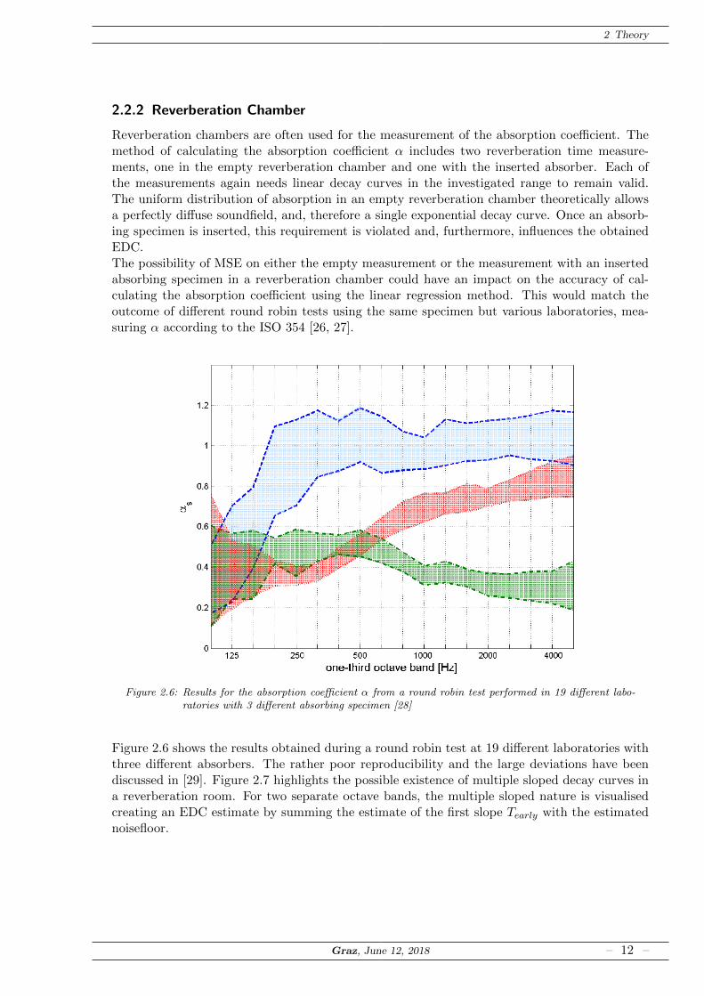
Reverberation chambers are often used for the measurement of the absorption coefficient. Themethod of calculating the absorption coefficient α includes two reverberation time measure-ments, one in the empty reverberation chamber and one with the inserted absorber. Each ofthe measurements again needs linear decay curves in the investigated range to remain valid.The uniform distribution of absorption in an empty reverberation chamber theoretically allowsa perfectly diffuse soundfield, and, therefore a single exponential decay curve. Once an absorb-ing specimen is inserted, this requirement is violated and, furthermore, influences the obtainedEDC.The possibility of MSE on either the empty measurement or the measurement with an insertedabsorbing specimen in a reverberation chamber could have an impact on the accuracy of cal-culating the absorption coefficient using the linear regression method. This would match theoutcome of different round robin tests using the same specimen but various laboratories, mea-suring α according to the ISO 354 [26, 27].

Figure 2.6: Results for the absorption coefficient α from a round robin test performed in 19 different labo-ratories with 3 different absorbing specimen [28]

Figure 2.6 shows the results obtained during a round robin test at 19 different laboratories withthree different absorbers. The rather poor reproducibility and the large deviations have beendiscussed in [29]. Figure 2.7 highlights the possible existence of multiple sloped decay curves ina reverberation room. For two separate octave bands, the multiple sloped nature is visualisedcreating an EDC estimate by summing the estimate of the first slope Tearly with the estimatednoisefloor.

Graz, June 12, 2018 – 12 –

2 Theory

0 0.2 0.4 0.6 0.8 1 1.2 1.4−40

−30

−20

−10

0

Dec

ayL

evel

(dB

)

EDCEstimate

1st slopeNoise

0 0.2 0.4 0.6 0.8 1 1.2 1.4−40

−30

−20

−10

0

Time (s)

Dec

ayL

evel

(dB

)

EDCEstimate

1st slopeNoise

Figure 2.7: Visualisation of an EDC and a single exponential fit summed with the estimated noisefloor plottedlogarithmically for the 250 Hz octave band (top) and the 4000 Hz octave band (bottom)

Considering these results and the previously described analytical aspects, new alternative toolsto extract multiple decay times from a given EDC become necessary.

Graz, June 12, 2018 – 13 –

2 Theory

2.3 The Decay rate Distribution

As derived in chapter 2.1.1 the sound field in an enclosure can be described as a sum of normalmodes of which each single one - after switching off the source - shows a single exponentiallydecaying motion. With this in mind and a bandpass filtered signal, the decay process for the Nexistent modes in the chosen frequency band can be described as [1]

p(t) =

N∑i=1

ai · e−δit cos (ωit− φi), (2.26)

where p(t) represents the sound pressure at a certain point in the room, ai the amplitudes ofeach excited mode and δi the decay constants. For a large number of N , the mean squaredsound pressure p2(t) follows as

p2(t) =1

2

N∑i=1

a2i · e−2δit. (2.27)

This sum is independent of the modes excited, hence, due to the large number N , interferingphenomena are cancelled and the varying decay constants create a discrete distribution. Trans-forming this discrete distribution into a continuous one and rewriting the sum in equation 2.27as an integral results in the energy density as a function of time for a particular point in theroom:

w(t) =

∫ ∞0

H(δ)e−2δtdδ (2.28)

with H(δ)dδ = D(δ)A(δ)dδ, where D(δ) represents the number of modes within the decayconstants of δ and δ + dδ and A(δ) denotes the amplitude of their excitation.After applying a variable transform 2t = p, the EDC can be regarded as the Laplace transformof its decay time distribution H(δ).

w(p

2

)=

∫ ∞0

H(δ)e−δpdδ = L{H(δ)} (2.29)

(a) Rectangular distribution (b) Two separate peaks

Figure 2.8: Common distributions with the corresponding calculated decay curves [1]

Graz, June 12, 2018 – 14 –

2 Theory

Considering a number of common distributions, examples of the resulting decay curves were pre-sented (see fig. 2.8). Every investigated distribution, except for a single peak or a rectangulardistribution with a width of α = 0, resulted in a multiple sloped decay curve.

Subsequently, Kutruff suggested in [1] to try calculating the decay rate distribution via theinverse Laplace transform of a given energy decay curve:

H(δ) = L−1{w(p

2

)}=

1

2πj

∫ j∞

−j∞w(p

2

)eδpdp =

1

π

∫ j∞

−j∞w(t)e2δtdt. (2.30)

Considering this analysis, Kuttruff made some important statements about the characteristicsof energy decay curves [1]:

◦ A semilogarithmically plotted decay curve can only be linear or concave. This conditiondoes not, in general, hold for coupled volume spaces.

◦ The early decay of a semilogarithmically plotted decay curve equals the weighted mean ofthe decay constants, the weight being the decayrate distribution.

◦ The commonly used method of fitting a linear regression to a certain interval might resultin severe errors.

Graz, June 12, 2018 – 15 –

2 Theory

2.4 Noise treatment

The measured room impulse response used for the further calculation includes some unavoidablenoise with the largest part being ambient and equipment noise. This especially becomes an issuewhen applying a Schroeder backwards integration or in the later step of trying to calculate T30

with a small SNR. To compensate this effect, the ISO 3382 [30] proposes three different methodsreviewed in [31]:

(1) Full Impulse Response: This approach takes the whole measured room impulse responseinto account, which means that no noise compensation is applied (see fig. 2.9a)

(2) Truncation: The second presented method truncates the RIR at the intersection time,the time where the signal’s energy drops below the mean noise level plus the variance ofthe noise process (see fig. 2.9b). For the data investigated and visualized in [31], thisintersection time was calculated using the Lundeby algorithm [32]. The truncation can bedescribed as a decrease of the upper bound of the integration interval for calculating theEDC, which results in a neglection of the remaining signal energy after the intersectiontime.

(a) Method (1): Full Impulse Response (b) Method (2): Truncation

Figure 2.9: Illustration of the calculation of the methods (1) and (2) [31]

(3) Correction for Truncation: The last algorithm compliant to the ISO 3382 uses the sameapproach as in (2) adding an exponentially decaying estimate for the remaining signalenergy (see fig. 2.10a). Considering a multi-exponential decay curve, the slope of thecomputed estimate from any given early part of the impulse respone would be too steepand create a non-concave EDC.

Furthermore, Guski reviews in [31] a noise subtraction method which was proposed by Chu in[33] and according to him results in the least artefacts when calculating an EDC.

(4) Subtraction of Noise Level: This procedure first calculates the squared room impulse re-sponse, followed by a subtraction of the estimated noisefloor before backwards integratingto obtain the desired EDC (see fig. 2.10b). To calculate the EDC all potentially negativevalues of the squared subtracted impulse response have to be forced to zero to keep thecharacteristics of a concave EDC. An additional disadvantage lies in an EDC approachingnegative infinity when regarded logarithmically. This approach is not compliant with theISO 3382.

Graz, June 12, 2018 – 16 –

2 Theory

(a) Method (3): Correction for Truncation (b) Method (4): Subtraction of Noise Level

Figure 2.10: Illustration of the calculation of the methods (3) and (4) [31]

Considering the development of an algorithm to extract reverberation times from a given EDC,a noise compensation method directly applied to the EDC seems more suitable. Therefore, onemore additional method is proposed.

(5) Subtraction of Noise Level (EDC): As the EDC is calculated by backwards integrating thesquared RIR (see eq. 2.25), the noise level can be estimated by computing the mean ofthe differential of the latter part of the EDC:

N =1

K

L−1∑n=Tint

EDC[n]− EDC[n+ 1] (2.31)

with K representing the number of samples between the intersection time Tint and the endof the given EDC in samples L. For the use without a search algorithm for the intersectiontime, a predefined length expected to be inside the noise floor can be used (e.g., 1.5 s untilthe end in fig. 2.11). This calculation method results in an adapted EDC which approachesa close to zero constant and, therefore, the benefit of a larger SNR.

0 0.5 1 1.5 2 2.5 3 3.5−50

−40

−30

−20

−10

0

Time (s)

Dec

ayL

evel

(dB

)

EDCEDC after noise subtraction

Figure 2.11: Comparison of the EDC calculated using method (1) and method (5)

Graz, June 12, 2018 – 17 –

3Methodologies

The upcoming chapter presents the theory behind the algorithms to be adapted. Each under-lying model is described explicitely to deepen the knowledge for the use in the latter parts.The selected algorithms were chosen according to three main goals previously stated in theintroduction. An additional fourth goal is introduced within this section.

(1) Underlying Model: The data used as input for the algorithm shows an exponentially decay-ing behaviour. Therefore, the output of the algorithms should be a set of the correspondingparameters A and T , creating the following underlying model:

yk(A, T, t) =∑i

Aie− tTi (3.1)

(2) Robustness: The implemented algorithm should possibly, considering a wide range ofdifferent EDC, find an accurate solution to the given problem.

(3) Minimising computation time: The implemented algorithm should represent a time effi-cient tool to calculate the decay times from a given EDC for practical purposes.

(4) Physical Relevance: The obtained solution should represent the physical characteristics ofan EDC.

3.1 VARPRO - Variable Projection Algorithm

The Variable Projection Algorithm is the first program to be investigated in this work. Thegeneral purpose of this method was to find the ”best” fit to an EDC using a predefined numberof exponentially decaying functions.The VARPRO algorithm presented by O’Leary & Rust [34] is a revised version of the 1973 pre-sented method by Golub and Pereyra [35]. This approach assumes that the underlying model isa linear combination of nonlinear functions [36]. Since the introduction of this method, a widevariety of applications were found and summarised in [37]. The exceptionally fast convergenceand, therefore, shorter computation times were often mentioned as a key reason for choosingVARPRO but with the following enhancements [38, 39, 40]. The simplicity of using a sum ofexponentials as the underlying model and having the possibility of implying an additional linearterm are the main reasons for choosing this version in this acoustical context. Furthermore,O’Leary & Rust proposed their implementation to be a 21st century implementation of thevariable projection concept using MATLAB [34].

Most nonlinear problems contain variables that are linear. Regarding the problem of a doublesloped energy decay curve, one can write the underlying model as

y(t) ≈ c1eα1t + c2e

α2t ≡ η(α, c, t), (3.2)

Graz, June 12, 2018 – 18 –

3 Methodologies

with y(t) being the experimental data. The parameter c in this case appears linear, which meansthat for a given set of α the optimal vector c can be found using a linear least squares algorithm.Hence, if the nonlinear problem is stated as

minα,c||y − η(α, c)||22 (3.3)

using a linear least squares approach to find the optimal values of c, equation 3.3 can be rewrittenas

minα,c||y − η(α, c(α))||22. (3.4)

Exploiting this property, Golub and Pereyra called this a separable least squares problem anddeveloped the variable projection method to solve it. The important step considering VARPROis the reduction of the parameters used in the minimisation problem. The implementation ofthis concept is rather complex and requires the calculation of the Jacobian matrix.Considering the experimental data y(t), the underlying nonlinear model could be written as

η(α, c, t) =n∑j=1

cjΦj(α, t) (3.5)

where the functions Φj denote the basis functions

Φ1(α, t) = eα1t ; Φ2(α, t) = eα2t. (3.6)

In this special implementation, an additional term with an independent parameter c can beused, but will not be considered in the derivation. For given experimental data regarding itsphysical fundamentals, it is often appropriate to have constraints on some parameters whichresults in the following minimisation problem

minα∈Sα

||W (y − η(α, c)) ||22 (3.7)

where c(α) solves the constrained linear least squares problem

minc∈Sc||W (y − Φc)) ||22. (3.8)

Using this basic idea, the program calls a state-of-the-art nonlinear least squares algorithm, sup-plying it with the Jacobian matrix of the full problem. A high-quality linear least squares solveris used. Additional statistical diagnostics from the solution are calculated to help evaluate thefound parameters. Furthermore, the linear and nonlinear least squares algorithms are external,so they can easily be exchanged by more suitable ones to meet some special needs.

Graz, June 12, 2018 – 19 –

3 Methodologies

3.2 RILT - Regularized Inverse Laplace Transform

RILT [41] is an emulation of the program CONTIN, which was proposed by Provencher in [42]as ”a general purpose constrained regularization program for inverting noisy linear algebraicand integral equations”. Marino used the publications explaining CONTIN [43] - [48] to builda thorough understanding about the algorithm and to reimplement it using MATLAB withoutknowing and understanding the original FORTRAN code [41]. As there is no further informationgiven by the author, all theoretical and practical background considered has been taken fromthe explanations about CONTIN except for some advice regarding the choice of the values ofsome user-defined variables according to [41].The data obtained in various experiments represents some linear integral transform of the wantedmeasure. E.g., a measured EDC can be regarded as the Laplace transform of the present decaytime distribution. The inversion of such data then is an ill-posed problem with an infiniteset of solutions [49]. Thus, a standard inversion principle can not be applied and statisticalregularisation methods have to be used [42]. The CONTIN algorithm tries to find an optimalsolution restricted to constraints. Prior statistical knowledge and the principle of parsimonyinfluence the regularizor. This approach increases the accuracy by decreasing the amount ofpossible artefacts caused by the experimental noise [47]. Yet the inverse problem is still ill-posedand the obtained solution remains one of the infinite set of possible solutions within experimentalerror.If the decay time distribution is considered the desired measure, and the measured EDC isregarded the indirectly obtained data, one can then describe the data set yk as a linear integraltransform of the decay time distribution with additional experimental noise:

yk = Φkx + νk (3.9)

For this particular problem, the linear operator would denote the kernel of the Laplace transform.

yk =

∫ b

aΦk(τ)H(τ)dτ +

NL∑i=1

Lkiβi + νk (3.10)

In this equation, Φk represents the kernel, H(τ) the decay time distribution and the sum statesthe possibility of CONTIN to handle an additional linear term. According to [47], there is anumber of causes which result in equation 3.10. For any given experiment, there might be morethan just one of the following reasons present.

(1) Imperfect input

(2) Imperfect detection

(3) Imperfect system

(4) Indirect measurement

(5) Multicomponent system

Regarding the above causes for an experiment to result in equation 3.10 and considering thecalculation of a decaytime distribution, one could deem all five reasonable. With todays mea-surement methods, the first two can be neglected but the latter three are all present.

Graz, June 12, 2018 – 20 –

3 Methodologies

(3) Imperfect system: The not perfectly diffuse soundfield in a reverberation room.

(4) Indirect measurement: The EDC has to be computed from the obtained RIR to thenobtain the problem ready for inversion.

(5) Multicomponent system: Considering the explanation in section 2.3, each component(mode) decays with a particular time constant. Thus, the sound field in an excited enclo-sure results in a multicomponent system.

Ignoring the optional linear term in equation 3.10, one can write the ill-posed problem as

yk =

∫ b

aΦk(τ)H(τ)dτ + νk. (3.11)

For the inversion of this formula, analytical inversion methods exist if νk = 0. By neglectingthe noise νk, one could also use this approach for inverting the noisy data obtained from themeasurement, but would then select one solution out of the set of infinitely many which wouldwith a high probability be a poor estimate. To find a possibly better estimate, CONTIN, bynumerical integration, first transforms equation 3.11 into a system of linear algebraic equations,

yk =

Ng∑m=1

cmΦ(τm)H(τm) + νk (3.12)

with Ng representing the number of predefined decay components chosen for the evaluationand cm denoting the weights of the quadrature formula. The amplitudes of H(τm) are thendetermined for each pre-defined decay time τm.

yk =

Nx∑j=1

Akjxj + νk (3.13)

With the step from equation 3.11 to equation 3.12, the previously ill-posed problem now posesan ill-conditioned problem. For finding the ”best” solution to the problem, CONTIN uses twoprinciples:

(1) Constraints: By having some absolute prior knowledge about the solution a large numberof possible solutions can be eliminated. Knowing, e.g., that the calculated EDC mustbe monotonically decreasing and concave (section 2.3), one can restrict the decay timedestribution to being non-negative.

(2) Regularisation: Having eliminated a lot of members of the solution space by applyingconstraints, still a large number of solutions within experimental error remain possible.Solving the now given weighted nonlinear least-squares problem

J = ||W−12

ν (y −Ax) ||2 = min, (3.14)

one would select one of the possible members and, therefore, still obtain a solution likelyto be far from the desired one. There are two strategies implemented in CONTIN thatcan be used as a combination or solely to approach the resulting problem of minimisingthe function with the additional regularisor:

J(α) = ||W−12

ν (y −Ax) ||2 + α2||r −Rx||2 = min (3.15)

Graz, June 12, 2018 – 21 –

3 Methodologies

◦ Statistical prior knowledge: In the special case of considering a room impulse responsemeasurement, no appropriate statistical prior knowledge about the solution could befound.

◦ Principle of parsimony: This principle by definition searches for the simplest solution,which can be understood as looking for a solution with the least additional informationto the one given by the constraints. As a result, the outcome should imply a minimalamount of artefacts. With no prior statistical knowledge, a good regularisor accordingto [47] is

||r −Rx||2 =

∫ b

a

(H ′′(τ)

)2dτ. (3.16)

For the usage with numerical integration to obtain equation 3.12, Provencher suggeststo set r = 0 and R = P with P being

P =

1−2 1 01 −2 1

. . . 1. . .

. . .

−2 10 1 −2

1

. (3.17)

This choice of the regularisor according to [47] is appropriate for the general purposeand results in a better suppression of extra isolated peaks than when using a maximumentropy regularisor.

Graz, June 12, 2018 – 22 –

3 Methodologies

3.3 MELT - Maximum Entropy Lifetime Analysis

The Maximum Entropy Lifetime Analysis tool presented in its updated version 4.0 by Shuklain [6] represents a program for the extraction of a lifetime distribution obtained from a positronlifetime experiment. Regarding an EDC as a lifetime spectrum allows the assumption of beingable to adapt the given algorithm in a way that it can be used for the extraction of decay timesfrom a given EDC.Considering this strategy of extracting a decay time distribution, the underlying model can bewritten similarly to the one in chapter 3.2

D(y) =

∫ b

aK(x, y)Φ(x)dx+N(y), (3.18)

with D(y) representing the measured data, K(x, y) being the kernel and N(y) the experimentalnoise with a known standard deviation σN . Thus, Φ(x) is the function to be obtained viaan inverse Laplace transform. The main discipline which gave rise to the development of thismethod was Positron Annihilation.With the notation used above and the use of a given EDC for the computational process,equation 3.18 can be rewritten as

D(t) =

∫ b

aK(τ, t)Φ(τ)dτ + ν(t), (3.19)

with the kernel K(τ, t) being τ−1etτ−1

, this results in

D(t) =

∫ b

a

(1

τetτ

)Φ(τ)dτ + ν(t) (3.20)

where Φ(τ) denotes the intensity as a function of the decay time. As the approach to solving thisequation is discrete and numerical, the transformation to a system of linear algebraic equationsis appropriate:

dj =

Nmod∑µ=1

kjµφµ + nj j = 1 · · ·Ndat (3.21a)

D = KΦ +N (3.21b)

To approach this problem, the MELT algorithm uses a quantified maximum entropy method.This method allows to find an estimate of a positive additive distribution (PAD) from noisy andincomplete data based on a Bayesian framework. ”Scientific data analysis should aim to inferresults from data in a logical manner.” [50] Hence, knowing a number of various solutions A,B, C, ... one could then describe them as conditional probabilities pr(A|D), pr(B|D), pr(C|D),... So if Φ was to represent a particular solution, one would need the probability distributionpr(Φ|D) subject to Φ. This is not directly obtainable from the given dataset D. However, thereversed conditioning pr(D|Φ) is, which is better known as the ”likelihood”. Assuming theexperimental noise to be uncorrelated and Gaussian, the probability density pG(N) with thenoise being described as N = D −KΦ would resolve as

Graz, June 12, 2018 – 23 –

3 Methodologies

pr(D|Φ) = pG(N) = pG(D −KΦ) = (3.22)

=

Ndat∏j=1

1√2πσ2

exp

− 1

2σ2

dj − Nmod∑µ=1

kjµφµ

2 (3.23)

Considering the calculation process for obtaining an EDC from a measured impulse response onehas to first look at the characteristics of the experimental noise in the impulse response beforedrawing conclusions for the EDC. The noise of the impuls response h(t) can be considereduncorrelated and Gaussian with zero mean which results in the above mentioned likelihoodfunction. Squaring the impulse response and furthermore using a cumulative summation theobtained noise in the EDC can be described as a central χ2-distribution with k degrees offreedom.

χ2k = L

(||U ||2

)= L (U1 + U2 + · · ·+ Uk) (3.24)

As the random vector U possesses a normal distribution L(U) = N(0, σk), the χ2-distributioncan be written as the squared norm of this Gaussian distribution

χ2k = ||Nk(0, σk)||2, (3.25)

with a probability density function (PDF) of

fk(x) =

[2k2 Γ

(k

2

)]−1

xk2−1e−

x2 , (3.26)

with Γ(x) denoting the gamma function

Γ(α) =

∫ ∞0

tα−1e−tdt. (3.27)

Reviewing each sample of the EDC, starting from the end and moving towards the beginningthe number of summed and squared random variables that are considered uncorrelated andGaussian increases by one with every step. Therefore, according to the central limit theorem(law of large numbers), after many steps (> 100), the χ2-distribution can be estimated by aGaussian distribution and equation 3.22 regains validity as the likelihood function for the noisein a given EDC [51]:

χ2k → N(0, σ) for n→∞ (3.28)

Graz, June 12, 2018 – 24 –

3 Methodologies

0 5 10 15 20 25 30 35 40 45 500

0.2

0.4

0.6

0.8

1

x

f k(x

)

k = 1k = 2k = 5k = 10k = 30

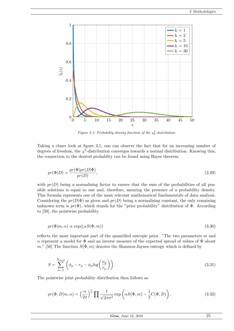
Figure 3.1: Probability density function of the χ2k-distribution

Taking a closer look at figure 3.1, one can observe the fact that for an increasing number ofdegrees of freedom, the χ2-distribution converges towards a normal distribution. Knowing this,the connection to the desired probablity can be found using Bayes theorem

pr(Φ|D) =pr(Φ)pr(D|Φ)

pr(D), (3.29)

with pr(D) being a normalising factor to ensure that the sum of the probabilities of all pos-sible solutions is equal to one and, therefore, assuring the presence of a probability density.This formula represents one of the most relevant mathematical fundamentals of data analysis.Considering the pr(D|Φ) as given and pr(D) being a normalising constant, the only remainingunknown term is pr(Φ), which stands for the ”prior probability” distribution of Φ. Accordingto [50], the pointwise probability

pr(Φ|m,α) ∝ exp((αS(Φ,m)) (3.30)

reflects the most important part of the quantified entropic prior. ”The two parameters m andα represent a model for Φ and an inverse measure of the expected spread of values of Φ aboutm.” [50] The function S(Φ,m) denotes the Shannon-Jaynes entropy which is defined by

S =

Nmod∑n=1

(φµ − rµ − φµlog

(φµrµ

)). (3.31)

The pointwise joint probability distribution then follows as

pr(Φ, D|m,α) =( α

2π

) r2∏ 1√

2πσ2exp

(αS(Φ,m)− 1

2C(Φ, D)

), (3.32)

Graz, June 12, 2018 – 25 –

3 Methodologies

which is proportional to the posterior probability by

pr(Φ|m,α,D) =pr(Φ, D|m,α)

pr(D|m,α). (3.33)

With the Shannon-Jaynes entropy being a convex function with negative definite curvature andC(f) being positive, the posterior probability pr(Φ|m,α,D) certainly has a unique maximum at

α∂S

∂Φ− 1

2

∂C

∂Φ= 0 at Φ = Φ. (3.34)

The obtained Φ then is the single most probable positive additive distribution.The choice of a well guessed kick-off solution is essential as it has a stabilizing and regularizingeffect. Furthermore, it shortens the convergence time. For this particular reason the MELTalgorithm uses a general optimal linear filter to compute a good kick-off solution. Designing afilter in this case means constructing a filter matrix F to solve the inverse problem by satisfyinga minimisation criterion. This is chosen to be the mean squared error between the real solutionΦ and the one extracted by the filter F [5]:

∑v

pv〈|F (KΦv −D)|2〉N = min (3.35)

As already described in section 3.2, it would be possible to directly minimise the mean squarederror between the data and the model, but this would not solve the inverse problem [5]. Toobtain the coefficients of the filter F the left side of equation 3.35 has to be differentiated withrespect to F and then equated to zero to satisfy the minimisation criterion. This leads to a filterF to obtain the regularised solution

Φr = FD, (3.36)

with

F =CΦK

T

KCΦKT + CN, (3.37)

where

CΦ =∑v

pvΦvΦTv ; CN = 〈NNT 〉. (3.38)

Graz, June 12, 2018 – 26 –

4MEDD - Maximum Entropy Decay Time

Distribution

The MEDD program is an adapted version of the previously explained MELT program. It usesthe methods described in section 3.3 to extract the decay time distribution from a given energydecay curve. This chapter will be used to give some insight into its structure and the function-ality. Furthermore, some advice on how to set the values of specific variables is given.

4.1 Structure

This program uses a set of subprograms to compute the desired distribution, which allows theuser to adapt the number of subprograms used - e.g., someone might not need to save or plot theresults - and, therefore, reduce the computation time. By choosing between two different mainprograms medd and medd loop, the user can furthermore choose between evaluating a singleEDC or a set of EDCs, each representing one frequency band out of the whole frequency rangechosen to be investigated.

medd medd loop

m input for i=1:Nf

m data

m tcmat

m pre

m iter

m res

while a > entwghtstop

m iter m res

m plot

m save

yes

no

Figure 4.1: Flow graph of the MEDD program using either medd or medd loop as the main program

Graz, June 12, 2018 – 27 –

4 MEDD - Maximum Entropy Decay Time Distribution

4.2 Subprograms

medd & medd loop

The scripts ”medd” and ”medd loop” represent the main programs and work as the trigger forall subprograms. If certain functions are supposed to be skipped during a particular calculation,one needs to comment those subprograms. The alternative of using medd as the main programis medd loop which is appropriate if the data set to be analyzed contains a number of EDCscorresponding to the EDCs of each octave or third octave frequency band.

m input

This file is the only one intended to be modified by the user. All variables specified previous tothe computational process are to be entered here. The defined values for the following variablesthen serve as input for m tcmat during the further process. Using medd loop, the whole coderelated to m input is included in the main program and therefore the file to input the user-defined values is also the main program. In this particular case, this eases the excitation anddata management.

� nameFile: Defines the data matrix to be loaded. MEDD supports two different formats:ASCII and MATLAB (.txt & .mat)

� nameDat: This variable should contain the name of the EDC chosen out of the ones savedin the data matrix.

� down: Downsampling is used to speed up the calculation. Considering a trade-off be-tween computation time and accuracy, a number between 10 and 100 is suggested. Thedownsampling factor chosen depends on the original sampling rate of the measurement. Aresulting downsampled sampling rate of fs < 24kHz should be avoided.

� origfs: The sampling frequency used when calculating the EDC should be stored in thisvariable.

� cutoff: The singular value cutoff is an important and critical variable when using MEDD.According to [6], it defines the size of the reduced system. The reduced system neglectsall singular values of the analysis matrix T that are smaller than the cutoff value. Thesmaller this value is chosen, the harder it is for the algorithm to converge. The go-to rangefor extracting decay times from a given EDC is 10−5 to 10−2. Generally, the largest valuewhich still gives a solution that represents the true nature of the EDC should be selected.

� entwghtstart / entwghtstop: These two values are the bounds for the variation of theentropy weight. In order to find a reasonable solution, the entropy should be close to zeroat these entropy weights and have its maximum inbetween. The bottom left part of thefirst plot created by m plot shows whether the range should be adapted or not. The limitsof the x-axis represent the values for entwghtstart and entwghtstop (see fig. 4.3 - a).

� enditer: This parameter defines the termination of the algorithm if no stabilized resultcould be found previous to the enditerth iteration step.

� Ntau / const / increment: These three values define the decay time range in samples.With const and increment, the shortest possible decay time to be analysed would be

τmin = exp

(const+

1

increment

)(4.1)

Graz, June 12, 2018 – 28 –

4 MEDD - Maximum Entropy Decay Time Distribution

and introducing Ntau the longest is then set to

τmax = exp

(const+

Ntau

increment

). (4.2)

m tcmat

During the execution of m tcmat, the analysis matrix for the extraction of the decay timedistribution is calculated. With the values defined in m input, the decay time grid is created byusing the following formula

τi = exp

(const+

i

increment

), (4.3)

with i ranging from 1 to Ntau. Using this grid, the analysis Matrix T incorporates all possibledecaying models, each of them stored in one column of T . The maximum intensity for eachmodel is normalized by the decay constant itself.

50 100 150 200 250 300 350−40

−35

−30

−25

−20

−15

−10

−5

0

Time (samples)

Inte

nsi

ty(d

B)

Figure 4.2: Visualisation of a anaylsis matrix T

If saveT = 1 in m input, the created analysis matrix will be stored. For any later calculation,this matrix can be used, which again reduces the time the algorithm takes to find a solution.

m pre

Running this script applies a linear filter to the data, as described in section 3.3. The resultingregularised solution ΦR is used as the kick-off solution for the iterative maximisation duringm iter. For further stabilisation, peaks with an intensity of less than one fifth of the maximum

Graz, June 12, 2018 – 29 –

4 MEDD - Maximum Entropy Decay Time Distribution

are neglected. This value is part of the CONTIN implementation and was considered appropri-ate after empirical testing.

m iter

This file represents the heart of the program. A quantified maximum entropy solution is calcu-lated in the singular value space by the algorithm proposed in [8]. To increase the stability, onlythe singular values of the T matrix that are larger than a specified cutoff value are considered.The iteration continues until either the maximum specified number of iterations is reached orthe χ2 value can not be reduced any further.

m res

Running m res prepares the obtained results to be plotted and/or saved. Furthermore, the co-variance matrix as a measure of the quality of the results is computed.

entropy variation loop

Following the described procedure a loop consisting of again m iter and m res is excited to findsolutions for different entropy weights. Starting at the given value of entwghtstart, with eachiteration step, the entropy weight is decreased according to

entwght = 10−0.1 · entwght (4.4)

until the defined value for entwghtstop is reached. During this procedure all obtained resultsare temporarely stored to be saved or plotted afterwards.

m plot & m save

Those two subprograms allow the user to visualize and/or save the results. m plot creates twofigures with detailed information about the iteration process, the result, the estimate and ofcourse the decay time distribution. The subplot on the right hand side of the second figurecreated by MEDD can be adapted to visualise the change of the decay time distribution withthe number of iterations instead of the variation as a function of the entropy weight (see fig. 4.3- b). m save can be used to save all parameters needed for a reproduction of the results into aMATLAB file.

Graz, June 12, 2018 – 30 –

4 MEDD - Maximum Entropy Decay Time Distribution

1 2 3 4 5 6 7 8 9 10 11

decay rates

0

0.05

0.1

0.15

0.2

0.25

0.3

0.35

0.4

0.45

0.5

no

rma

lize

d in

ten

sity

highest entropy solution

10 -10 10 -9 10 -8 10 -7 10 -6 10 -5

entropy weight

0

0.02

0.04

0.06

0.08

0.1

0.12

0.14

0.16

0.18

0.2

pro

ba

bili

ty

700 750 800 850 900 950 1000

log(TAU)

5

10

15

20

25

30

35

40

45

50

log

(en

twe

igh

t)

solution variation with ent. weight

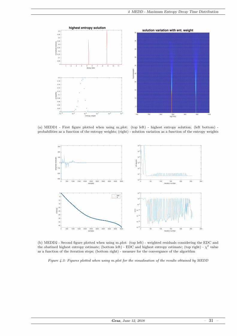
(a) MEDD1 - First figure plotted when using m plot: (top left) - highest entropy solution; (left bottom) -probabilities as a function of the entropy weights; (right) - solution variation as a function of the entropy weights

0 500 1000 1500 2000 2500 3000 3500 4000 4500 5000

samples

-300

-200

-100

0

100

200

300

we

igh

ted

re

sid

ua

ls

0 50 100 150 200 250 300

iteration number

10 0

10 1

10 2

10 3

10 4

10 5

10 6

ch

i sq

ua

re

0 500 1000 1500 2000 2500 3000 3500 4000 4500 5000

samples

-45

-40

-35

-30

-25

-20

-15

-10

-5

0

inte

nsity

data

fit

0 50 100 150 200 250 300

iteration number

10 -25

10 -20

10 -15

10 -10

10 -5

10 0

10 5

co

nv

(b) MEDD2 - Second figure plotted when using m plot: (top left) - weighted residuals considering the EDC andthe obatined highest entropy estimate; (bottom left) - EDC and highest entropy estimate; (top right) - χ2 valueas a function of the iteration steps; (bottom right) - measure for the convergance of the algorithm

Figure 4.3: Figures plotted when using m plot for the visualisation of the results obtained by MEDD

Graz, June 12, 2018 – 31 –

5Measurement Conditions

All upcoming sections use experimental data to investigate the multiple sloped effect of a specificreverberation chamber. All data was provided by Jamilla Balint who carried out the measure-ments at the DTU (Danmarks Tekniske Universitet) in Lyngby (Denmark). The upcomingchapter describes the measurement setup and all steps to obtain the EDCs, which are used asthe input for the different algorithms.

5.1 Measurement Setup

The rectangular reverberation chamber has a total volume of 241.6 m3 with side lengths of 4.91x 6.26 x 7.86 m. All walls are parallel and considered lightly damped.

Figure 5.1: Floor plan of the reverberation room with all receiver and source positions marked and an exem-plaric absorber setup

Graz, June 12, 2018 – 32 –

5 Measurement Conditions

Figure 5.1 shows a floor plan of the chamber with microphone and loudspeaker positions. Theimpulse responses were measured at four different receiver positions with three different sourcepositions which results in twelve independent measurements.

5.2 Diffusors and Absorbers

If scattering objects were introduced, 6 or 20 acrylic glass panels respectively were hung fromthe ceiling in a random configuration. The investigated absorbing specimen were made out ofglass wool with a thickness of d = 100 mm and a flow resistivity of σ = 12.9 kPas/m2. Theabsorbers were mounted on the floor according to ISO 354 [52] with covered side walls and noair gap (see fig. 5.2).

(a) 5 absorber (b) 15 absorber

Figure 5.2: Picture of the measurement setup with 5 and 15 absorbers introduced

Figure 5.2 shows the absorber setups whose measured impulse responses were selected for furthercalculations. Additionally to that the empty room measurement was considered. This selectiononly treats measurements according to the ISO 354.

Graz, June 12, 2018 – 33 –

5 Measurement Conditions

5.3 Calculation of the EDC

The gained impulse responses were either filtered in octave or third-octave bands before squaringand performing a Schroeder backwards integration to obtain the desired energy decay curves.Each EDC has then been reviewed before being considered for the averaged EDC of all 12combinations of receiver and source positions for each measurement. The resulting matricescontaining the averaged EDCs of each frequency band for one measurement were stored usingthe filenames shown in table 5.1 and 5.2.

Number of Absorbers

Number of Diffusors 0 5 15

0 0diff empty.mat 0diff 5abs.mat 0diff 15abs.mat6 6diff empty.mat 6diff 5abs.mat 6diff 15abs.mat

20 20diff empty.mat 20diff 5abs.mat 20diff 15abs.mat

Table 5.1: Nomenclature for the stored matrices containing the EDCs for each frequency band (octaves)

Number of Absorbers

Number of Diffusors 0 5 15

0 0diff empty3.mat 0diff 5abs3.mat 0diff 15abs3.mat6 6diff empty3.mat 6diff 5abs3.mat 6diff 15abs3.mat

20 20diff empty3.mat 20diff 5abs3.mat 20diff 15abs3.mat

Table 5.2: Nomenclature for the stored matrices containing the EDCs for each frequency band (third-octaves)

Graz, June 12, 2018 – 34 –

6Test Cases

In the upcoming chapter, case studies for the three implemented algorithms are presented. Thecharacteristics and suitability of each of the programs for the extraction of decay times anddecay time distributions from a given measured EDC is discussed. All data investigated in thischapter were obtained during the measurement described in chapter 5. A description of the datasets used to create each of the figures shown in this section can be found in the Appendix (p. 68).

6.1 VARPRO

Using the VARPRO algorithm for the calculation of the reverberation time is a time efficientalternative to the conventional method of fitting a linear regression in a least squared errorsense between the starting point at 0 dB or -5 dB and the point where the sound decay leveldrops below -10, -15, -20 or -30 dB depending on the SNR of the measured data. Except of theapplication of a downsampling to reduce the calculation time and at the same time the size ofthe storage needed, there are no further precalculations used. The downsampling does not affectthe result as it is comparable to a smoothening of the decay curve with the whole frequencyinformation already being transferred to the EDC.

6.1.1 Single slope estimation

A slightly adapted version of the VARPRO algorithm is used to calculate the reverberation timeof a given EDC. With the number of nonlinear terms set to one, the resulting model shows thefollowing behaviour:

MOD = A1 · e−13.8 t

T1 +N (6.1)

where A1 and T1 represent the corresponding amplitude and decay time respectively and Ndenotes the noise. The noise term that occurs when summing up and backwards integratingthe actual experimental noise existent in the room impulse response creates an additional linearterm in the EDC and does not correspond to the constant term as stated in the model equation6.1. The gradient of this linear term is therefore calculated analogous to equation 2.31.Using this method for the calculation of the reverberation time, one can compute a ratheraccurate value for the first part of the EDC. Considering a double sloped EDC, this strategyneeds no further knowledge about the turning point. The single sloped VARPRO estimates resultin a larger error for the latter part of the decay process but represent an accurate estimate forthe first part (see fig. 6.1). No appropriate comparison for the commonly used method and thesingle slope VARPRO can be made, as the old method does not represent the true nature ofany part of the decay curve but might possibly result in a smaller mean squared error.

Graz, June 12, 2018 – 35 –

6 Test Cases

0 0.1 0.2 0.3 0.4 0.5 0.6 0.7 0.8 0.9 1 1.1 1.2 1.3 1.4−40

−30

−20

−10

0

Time (s)

Dec

ayL

evel

(dB

)

EDCT20 slopeVARPRO estimate

1st slopeNoise

Figure 6.1: Single slope estimation for a double sloped EDC using VARPRO with an automated noisefloorestimation (20 diffusors, 15 absorbers, 250 Hz octave band)

Using the previously explained noise subtraction method to increase the SNR of the EDC, therange for the linear regression method of calculating the reverberation time can be increased.Calculations that result in a large SNR are assumed to be more accurate but for this particularcase (see fig. 6.1 and 6.2), this results in a flatter estimate due to a part of the second slopeblurring the perception. This means that the second slope is now chosen to be the main decayingcomponent.

0 0.1 0.2 0.3 0.4 0.5 0.6 0.7 0.8 0.9 1 1.1 1.2 1.3 1.4−50

−40

−30

−20

−10

0

Time (s)

Dec

ayL

evel

(dB

)

EDCT30 slopeVARPRO estimate

1st slopeNoise

Figure 6.2: Single slope estimation for a double sloped EDC using VARPRO with an automated noise sub-traction (20 diffusors, 15 absorbers, 250 Hz octave band)

Graz, June 12, 2018 – 36 –

6 Test Cases

6.1.2 Multiple slope estimation

To extract multiple decay times from a given EDC, the adapted VARPRO algorithm could pos-sibly be a great choice. Nevertheless, when choosing a certain number of exponential terms thatis larger than one, the algorithm will find a solution that is within experimental noise, but doesin most cases not represent the true nature of the EDC. For an EDC with heavy fluctuationsin the first five dezibel drop, this results in a fit where the first decay time is random and fartoo short. The second slope would then describe Tearly (see figure 6.4) or in the case of a singlesloped EDC the reverberation time (see figure 6.3). For this special case, the ISO 3382 [30] sug-gests a start of the evaluation at L = −5dB. Applying this strategy results in a good estimatefor the first slope and a mostly slightly off second.

0 1 2 3 4 5 6 7 8 9 10 11 12−40

−30

−20

−10

0

Time (s)

Dec

ayL

evel

(dB

)

EDCVARPRO estimate

1st slope

2nd slopeNoise

Figure 6.3: Double slope estimation of single sloped data using VARPRO with an automated noisefloorestimation (20 diffusors, 0 absorbers, 250 Hz octave band)

0 1 2 3 4 5 6 7 8 9 10 11 12−40

−30

−20

−10

0

Time (s)

Dec

ayL

evel

(dB

)

EDCVARPRO estimate

1st slope

2nd slopeNoise

Figure 6.4: Double slope estimation of double sloped data using VARPRO with an automated noisefloorestimation (20 diffusors, 0 absorbers, 500 Hz octave band)

Graz, June 12, 2018 – 37 –

6 Test Cases

0 2 4 6 8 10 12 14 16 18 20−50

−40

−30

−20

−10

0

Time (s)

Dec

ayL

evel

(dB

)

EDCVARPRO estimate

1st slope

2nd slopeNoise

Figure 6.5: Double slope estimation of double sloped data using VARPRO with an automated noisefloorestimation starting at -5dB (0 diffusors, 0 absorbers, 125 Hz octave band)

Considering a double sloped EDC where Tearly can be identified in both cases - starting atL = 0dB (fig. 6.6) and L = −5dB (fig. 6.5) - the resulting values of the reverberation times aresimilar but the intensity of the second slope is overestimated by the version, which is using thewhole EDC. For the evaluation starting at L = −5dB a visually more accurate result is gained.Furthermore, the accuracy of the obtained values is strongly depending on the turning pointbetween the two slopes, as a bend inside the first 5 dB drop would be neglected by the methodcompliant with the standard.

0 2 4 6 8 10 12 14 16 18 20−50

−40

−30

−20

−10

0

Time (s)

Dec

ayL

evel

(dB

)

EDCVARPRO estimate

1st slope

2nd slopeNoise

Figure 6.6: Double slope estimation of double sloped data using VARPRO with an automated noisefloor (0diffusors, 0 absorbers, 125 Hz octave band)

Graz, June 12, 2018 – 38 –

6 Test Cases

If the intersection point of the first and the second existing slope would be located in the first5 dB drop, the EDC evaluated would then become single sloped and therefore the algorithmwould fail to converge.Figure 6.7 shows a close to perfect estimation of the given EDC. Finding a solution like this byusing the adapted VARPRO algorithm happens on a random basis.

0 0.5 1 1.5 2 2.5 3 3.5 4−50

−40

−30

−20

−10

0

Time (s)

Dec

ayL

evel

(dB

)

EDCVARPRO estimate

1st slope

2nd slopeNoise

Figure 6.7: Double slope estimation of double sloped data using VARPRO with an automated noisefloor (0diffusors, 0 absorbers, 500 Hz octave band)

6.1.3 Results

The VARPRO algorithm in the version by O’Leary & Rust [34] was slightly adapted to meet theneeds of investigating energy decay curves. Nevertheless, considering the previously explainedexamples, the program is no appropriate tool for extracting decay times from a given EDC. Forcertain data sets with a clearly visible double sloped behaviour, the algorithm will find randomsolutions that mostly don’t represent the true nature of the decay curve. Due to the ill-posednessof the problem, the obtained solution does in fact solve the problem but might not be the onethat is physically the most reasonable. The necessity to define the number of non-exponentialterms previous to triggering the start of the program shows a huge handicap, especially if thefirst slope in the EDC could be either the first or the second one identified by the algorithm(see figure 6.3). Applying the method of neglecting the first 5 dB drop as proposed in ISO 3382[30], one neglects an important part of the decay curve [1]. Furthermore, if the turning pointwas inside the neglected part, a single sloped EDC is reviewed instead of a double sloped one,which completely fails the desired purpose and causes the algorithm to abort.Yet it is possible to obtain accurate results for the early decay time Tearly by using VARPROwith only one exponential term to fit the first identifiable slope. This gives a useful applicationfor this program, but does not at all correspond to the wanted extraction of the decay times ofmultiple slopes.Due to the identified poor performance of this algorithm, no further improvements concerningthe usability were implemented and the further search for a more robust algorithm was carriedout using the approach via an inverse Laplace transform.

Graz, June 12, 2018 – 39 –

6 Test Cases

6.2 RILT

Using the RILT program for the extraction of reverberation times from a given EDC meansspecifying a linear or logarithmic grid of decay times which is then fitted to the energy decaycurve as a sum of exponential models. The outcome is a discrete decay time distribution whichrepresents the obtained intensities for all predefined decay times.

0 2 4 6 8 10 12 14 16 18 20

−50

−40

−30

−20

−10

0

Time (s)

Dec

ayL

evel

(dB

)

Data and Fitting

EDCEstimate

0 2 4 6 8 10 12 14 16 18 20 22 24 26 28 300

5 · 10−2

0.1

0.15

0.2

Decay Time (s)

Norm

aliz

edIn

ten

sity

Reverberation Time Distribution H(RT)

Figure 6.8: Plots illustrating the results generated by RILT when investigating a given EDC (0 diffusors, 0absorbers, 4000 Hz octave band)

Reviewing the decay time distribution in figure 6.8, various decay times can be observed as thereis more than just one single peak present. Due to the small number N = 50 of evaluated decaytimes and the resulting coarse grid it is difficult to determine a certain number of peaks in thedecay time distribution. The possibility to use either a logarithmic or a linear grid gives onethe opportunity to first narrow the range of available decay times by applying a logarithmicgrid, followed by obtaining a more accurate result when using a smaller linear stepsize duringa second calculation. The closer grid points make it possible for the algorithm to find a moredistribution-like solution with two separate maxima (see fig. 6.9).

Graz, June 12, 2018 – 40 –

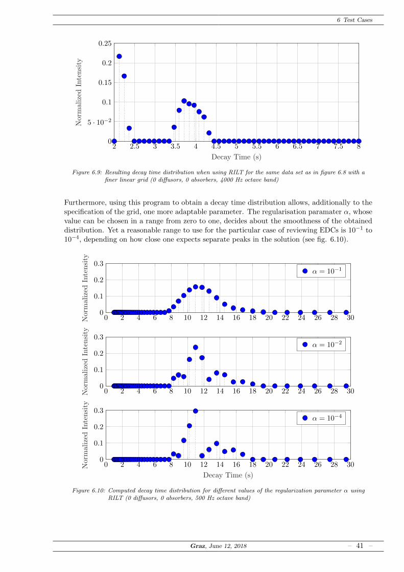
6 Test Cases

2 2.5 3 3.5 4 4.5 5 5.5 6 6.5 7 7.5 80

5 · 10−2

0.1

0.15

0.2

0.25

Decay Time (s)

Nor

mal

ized

Inte

nsi

ty

Figure 6.9: Resulting decay time distribution when using RILT for the same data set as in figure 6.8 with afiner linear grid (0 diffusors, 0 absorbers, 4000 Hz octave band)

Furthermore, using this program to obtain a decay time distribution allows, additionally to thespecification of the grid, one more adaptable parameter. The regularisation paramater α, whosevalue can be chosen in a range from zero to one, decides about the smoothness of the obtaineddistribution. Yet a reasonable range to use for the particular case of reviewing EDCs is 10−1 to10−4, depending on how close one expects separate peaks in the solution (see fig. 6.10).

0 2 4 6 8 10 12 14 16 18 20 22 24 26 28 300

0.1

0.2

0.3

Nor

mal

ized

Inte

nsi

ty

α = 10−1

0 2 4 6 8 10 12 14 16 18 20 22 24 26 28 300

0.1

0.2

0.3

Nor

mal

ized

Inte

nsi

ty

α = 10−2

0 2 4 6 8 10 12 14 16 18 20 22 24 26 28 300

0.1

0.2

0.3

Decay Time (s)

Nor

mali

zed

Inte

nsi

ty

α = 10−4

Figure 6.10: Computed decay time distribution for different values of the regularization parameter α usingRILT (0 diffusors, 0 absorbers, 500 Hz octave band)

Graz, June 12, 2018 – 41 –

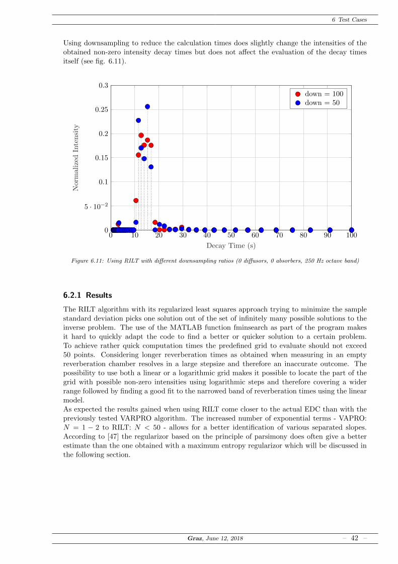
6 Test Cases

Using downsampling to reduce the calculation times does slightly change the intensities of theobtained non-zero intensity decay times but does not affect the evaluation of the decay timesitself (see fig. 6.11).

0 10 20 30 40 50 60 70 80 90 1000

5 · 10−2

0.1

0.15

0.2

0.25

0.3

Decay Time (s)

Nor

mal

ized

Inte

nsi

ty

down = 100down = 50

Figure 6.11: Using RILT with different downsampling ratios (0 diffusors, 0 absorbers, 250 Hz octave band)

6.2.1 Results

The RILT algorithm with its regularized least squares approach trying to minimize the samplestandard deviation picks one solution out of the set of infinitely many possible solutions to theinverse problem. The use of the MATLAB function fminsearch as part of the program makesit hard to quickly adapt the code to find a better or quicker solution to a certain problem.To achieve rather quick computation times the predefined grid to evaluate should not exceed50 points. Considering longer reverberation times as obtained when measuring in an emptyreverberation chamber resolves in a large stepsize and therefore an inaccurate outcome. Thepossibility to use both a linear or a logarithmic grid makes it possible to locate the part of thegrid with possible non-zero intensities using logarithmic steps and therefore covering a widerrange followed by finding a good fit to the narrowed band of reverberation times using the linearmodel.As expected the results gained when using RILT come closer to the actual EDC than with thepreviously tested VARPRO algorithm. The increased number of exponential terms - VAPRO:N = 1 − 2 to RILT: N < 50 - allows for a better identification of various separated slopes.According to [47] the regularizor based on the principle of parsimony does often give a betterestimate than the one obtained with a maximum entropy regularizor which will be discussed inthe following section.

Graz, June 12, 2018 – 42 –

6 Test Cases

6.3 MEDD

The quantified maximum entropy method used by the MEDD program represents a time effi-cient alternative to the RILT algorithm with a probabilistic choice of the solution. This adaptedalgorithm is considered the go-to algorithm for the further investigations concerning MSE in areverberation chamber.

6.3.1 Evaluation of extracted decay times

Evaluating the performance of the MEDD program represents a difficult task, as the commonway of using synthetic data to see whether the extracted decay times exactly match the decaytimes of the specified curve is disadvised in [6]. The obtained averaged solution gives a smoothrepresentation and therefore is not really suitable for the extraction of discrete decay times. Us-ing a low entropy weight solution results in sharper peaks and thus in a more accurate fit for thisparticular case but should be handled with care, as this solution uses only a rough regularisationand could therefore incorporate artefacts. It is not the algorithms purpose to extract discretedecay times as most decaying processes in nature present a distribution of decay times.As the VARPRO algorithm finds an accurate fit for the first slope of the decay curve whenfitting a single exponential term, this estimate is used to evaluate the extracted decay times ofthe first peak calculated by MEDD.

Octave band Number of slopes Tearly - VARPRO Tfirst - MEDD Tsecond - MEDD

250Hz 2 6.20s 5.01s 7.11s500Hz 1 5.61s 5.56s -

1000Hz 1 4.43s 4.44s -2000Hz 2 2.75s 2.52s 3.56s4000Hz 2 1.49s 1.16s 1.83s8000Hz 2 0.78s 0.76s 1.29s

Table 6.1: Decay times calculated by VAPRO and MEDD

Table 6.1 shows a comparison of the decay times extracted by the two different algorithms,VARPRO and MEDD. The decay times obtained by VARPRO were calculated using a singleexponential model. The stated decay times Tfirst and Tsecond represent the peaks of the decay-time distributions calculated using MEDD. In none of the shown frequency bands, a number ofslopes greater than two (N > 2) could be observed. For a single sloped behaviour (500 Hz and1000 Hz) the extracted decay times show little deviation. For frequency bands in which MEDDdetected a double sloped nature, the decay times of the VARPRO algorithm are often placedbetween the two different gradients obtained by MEDD (250 Hz, 2000 Hz, 4000 Hz). Dependingon the intensities of the two peaks present in the MEDD solution, the VARPRO solution canbe closer or further from the first slope obtained by MEDD. This behaviour of the VARPROalgorithm can be described as an unwanted averaging between the two existing slopes.

Graz, June 12, 2018 – 43 –

6 Test Cases

6.3.2 Variation of user specified variables

In addition to the above mentioned evaluation of the extracted decay times, variations of theuser-specified variables have been performed to give a rough overview about the robustness ofthis algorithm.

7.5 8 8.5 9 9.5 10 10.5 11 11.5 120

0.2

0.4

0.6

Decay Times (s)

Nor

mal

ized

Inte

nsi

ty

N = 690N = 700N = 750N = 800N = 1000N = 1200

Figure 6.12: Illustration of the effect of varying the user specified variable Ntau on the resulting decay timedistribution for a double sloped EDC (0 diffusors, 0 absorbers, 1000 Hz octave band)

The first analysis considers the variation of Nτ . In figure 6.12 slight differences in the positionof the peaks of the distribution can be obtained. For a large value of Nτ the distribution seemsto stabilise. This behaviour can be observed in all investigated data sets which results in thesuggestion to choose the value for Nτ twice the longest expected decay time to obtain a stabilisedsolution. If the upper limits for the extracted decay times Nτ is chosen close to the real longestdecay time or even below, the algorithm will fail to converge.Varying the paramater increment means varying the stepsize of the grid produced to analyze thedata. Hence, a smaller value for increment results in a coarser grid and thus means obtaining aless accurate solution. Reviewing the results for an increase of this parameter, no serious increaseof the computation time can be noticed and therefore a larger value seems reasonable. To obtaina comparable plot with same stepsizes an interpolation has been performed on the solutions witha smaller value for increment (see fig. 6.13). The negative values for the normalized intensityare artefacts resulting from the interpolation process.

7.5 8 8.5 9 9.5 10 10.5 11 11.5 12

0

0.2

0.4

0.6

Decay Times (s)

Nor

mal

ized

Inte

nsi

ty

i = 100i = 150i = 200i = 400

Figure 6.13: Illustration of the effect of varying the user specified variable increment on the resulting decaytime distribution for a double sloped EDC (0 diffusors, 0 absorbers, 1000 Hz octave band)

Graz, June 12, 2018 – 44 –

6 Test Cases

Changing the last remaining variable const that influences the decay time grid does not affectthe distribution at all. Neither the intensities nor the location of the peaks change, as long asthere is enough space between the shortest decay time possible in the EDC and the shortestdecay time present in the analysis matrix T .As explained in section 3.3, the values for the parameters endwgthstart and entwghtstop shouldbe chosen in a way that the entropy of the different solutions when varying the entropy weightis equal to zero at endwgthstart and endwgthstop but has a maximum inbetween. A possiblefunction subject to the entropy weight can be seen in figure 6.14. The values for entwghtstartand endwghtstop represent the lower and upper limit of the plot respectively.

10−10 10−9 10−8 10−70

5 · 10−2

0.1

0.15

0.2

0.25

Entropy weight

Pro

bab

ilit

y

Figure 6.14: Illustration to correctly choose the values for endwgthstart and endwgthstop (0 diffusors, 0absorbers, 1000 Hz octave band)

6.3.3 Results

Investigating its behaviour, MEDD seems to be the most reliable of the three implementedmethods for extracting decay times from a given EDC. Furthermore, it leaves the least squaresapproach and tries to find a most probable solution. A more detailed comparison of RILT andMEDD can be found in the next section. The highest entropy solution often shows rather sharppeaks. To be able to consider a wider set of solutions MEDD can also calculate the averagedsolution of all non-zero entropy solutions. This smoother solution should be considered if thehighest entropy solution does not represent the true nature of the given problem.

Graz, June 12, 2018 – 45 –

6 Test Cases

6.4 MEDD vs. RILT

As both of the mentioned algorithms try to extract the decay time distribution from a givendecay curve, a good choice for evaluating either of them is by comparing them. The authors of[53] present a comparison of the underlying methodologies, implemented as MELT and CONTINand used in the field of positron lifetime spectroscopy. A huge benefit of the MEDD algorithmcompared to the RILT are the short computation times when using a fine decay time grid.MEDD can find a solution in about the same time as RILT using ten times the amount ofgridpoints. As there is no possibility to run a decay time distribution calculation with RILT anduse as many points as suggested for MEDD without weeklong computation times, the resolutionof the obtained decay time distribution when using RILT always presents a handicap.

6.4.1 Single sloped EDCs

10 10.2 10.4 10.6 10.8 11 11.2 11.4 11.6 11.8 120

0.1

0.2

0.3

0.4

0.5

0.6

0.7

0.8

Decay Time (s)

Nor

mal

ized

Inte

nsi

ty

RILTMEDD

Figure 6.15: Decay time distributions calculated by RILT and MEDD for a single sloped EDC (20 diffusors,0 absorbers, 500 Hz octave band)

In figure 6.15, the solution obtained by MEDD shows one sharp peak and therefore, as thegiven EDC can be considered single sloped, gives a better estimate than the RILT estimate.Due to several peaks with a smaller amplitude in the RILT solution, it is hard to detect themain reverberation time by just looking at the figure, but using the maximum of each solution’sdistribution as the single reverberation time results in figure 6.16. Reviewing the completeresults as plotted by m plot, one can observe a slightly wider distribution for smaller entropyweights (see fig. 4.3). In figure 6.16 the MEDD estimate represents the EDC well for a longpart of the EDC. After a certain point, a sligthly different decay time is present and wouldtherefore create a double sloped effect. With RILT overestimating this second part, the overallmean squared error is smaller for the MEDD estimate.

Graz, June 12, 2018 – 46 –

6 Test Cases

0 2 4 6 8 10 12 14−40

−30

−20

−10

0

Time (s)

Dec

ayL

evel

(dB

)

EDCRILT estimateMEDD estimateNoise

0 2 4 6 8 10 12 14−2

−1

0

1

2·10−2

Time (s)

Res

idu

als

RILTMEDD

Figure 6.16: Illustration of estimates and residuals for a given measured EDC. Estimates are calculated byusing the maximum of each decay time distribution (RILT, MEDD) to create a single exponen-tial decay curve added to the estimated noise floor. (20 diffusors, 0 absorbers, 500 Hz octaveband)

6.4.2 Multiple sloped EDCs

The same process as described in the previous section for investigating single sloped decay curvesis now used for multiple sloped EDCs. Regarding this particular case, the possibility to use afine linear grid with a narrow range for a second calculation when working with RILT becomesdifficult, as with a multiple sloped decay curve, the range can not be reduced as far as for asingle sloped EDC. In figure 6.17, the small stepsize using MEDD can be seen. Having no closeto perfect representation of the reverberation time due to the coarse grid, the RILT algorithmtherefore has to use more separate peaks to find a good fit to the EDC. With the many localmaxima present in this distribution, it is hard to find a double or triple sloped estimate to theEDC as one would then have to select certain peaks and therefore neglect others.

Graz, June 12, 2018 – 47 –

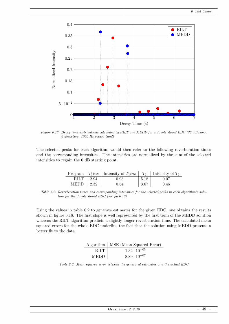
6 Test Cases

1 2 3 4 5 6 70

5 · 10−2

0.1

0.15

0.2

0.25

0.3

0.35

0.4

Decay Time (s)

Nor

mal

ized

Inte

nsi

ty

RILTMEDD

Figure 6.17: Decay time distributions calculated by RILT and MEDD for a double sloped EDC (20 diffusors,0 absorbers, 4000 Hz octave band)

The selected peaks for each algorithm would then refer to the following reverberation timesand the corresponding intensities. The intensities are normalized by the sum of the selectedintensities to regain the 0 dB starting point.

Program T1ins Intensity of T1ins T2 Intensity of T2

RILT 2.94 0.93 5.18 0.07MEDD 2.32 0.54 3.67 0.45

Table 6.2: Reverberation times and corresponding intensities for the selected peaks in each algorithm’s solu-tion for the double sloped EDC (see fig 6.17)

Using the values in table 6.2 to generate estimates for the given EDC, one obtains the resultsshown in figure 6.18. The first slope is well represented by the first term of the MEDD solutionwhereas the RILT algorithm predicts a slightly longer reverberation time. The calculated meansquared errors for the whole EDC underline the fact that the solution using MEDD presents abetter fit to the data.

Algorithm MSE (Mean Squared Error)

RILT 1.32 · 10−05

MEDD 8.89 · 10−07

Table 6.3: Mean squared error between the generated estimates and the actual EDC

Graz, June 12, 2018 – 48 –

6 Test Cases

0 0.5 1 1.5 2 2.5 3 3.5 4−30

−25

−20

−15

−10

−5

0

Time (s)

Dec

ayL

evel

(dB

)

EDCRILT estimateMEDD estimateNoise

0 0.5 1 1.5 2 2.5 3 3.5 4−4

−2

0

2

4·10−2

Time (s)

Res

idu

als

RILTMEDD

Figure 6.18: Illustration of estimates and residuals to a given EDC. Estimates are calculated by using themaxima of the selected peaks from each decay time distribution (RILT, MEDD) to create a multi(double) exponential decay curve added to the estimated remaining noise floor. (20 diffusors,0 absorbers, 4000 Hz octave band)

Graz, June 12, 2018 – 49 –

7Results

The upcoming chapter discusses the results obtained using the implemented algorithms. First,the bottom end of the measured frequency spectrum, represented by the 25 Hz third octave bandis investigated. The following section highlights the differences of using third octave or octavebands for the calculation. Subsequently, by reviewing the decay time distributions obtainedwith MEDD for different absorber and diffusor scenarios, the changes regarding the number ofslopes present in an EDC are investigated.

7.1 The 25 Hz band

For the investigated reverberation chamber, the 25 Hz band ranging from 22.4 Hz to 28.2 Hz(see table A.1) only incorporates one normal mode.

f0−1−0 =c

2

√(0

lx

)2

+

(1

ly

)2

+

(0

lz

)2

=c

2

√(1

6.26m

)2

= 27.4Hz (7.1)

This axial mode propagating in the y-direction of the specified coordinate system (see figure 2.1)can be described as a standing wave with the following sound pressure distribution (see fig. 7.1).

0 0.1 0.2 0.3 0.4 0.5 0.6 0.7 0.8 0.9 10

0.2

0.4

0.6

0.8

1

Relative distance (y-direction)

Ab

solu

teso

un

dpre

ssu

re

Figure 7.1: Absolute sound pressure distribution for the 0-1-0 axial mode

Considering this sound pressure distribution, a measurement position closer to the middle of theroom (y-direction) would then result in an EDC with a much worse SNR than at a measurementposition closer to the wall. Before the spatial averaging of the EDC, the calculated EDC for eachmeasurement position is normalized such that every EDC starts at zero dezibel. Investigating

Graz, June 12, 2018 – 50 –

7 Results

the noisefloor of the now normalized EDCs, one can observe major differences. The obtaineddecay curves form groups as shown in figure 7.2. Each group represents a measurement positionand the different curves of each measurement position then stand for the different loudspeakerpositions. For the groups of the measurement positions M1 and M4 the signal does not separatefrom the ambient noise and the EDC mostly represents a normalized noise floor. These are thetwo microphone positions closer to the middle of the room (y-direction).

0 2 4 6 8 10 12 14 16 18 20−40

−30

−20

−10

0

Dec

ayL

evel

(dB

)

0 2 4 6 8 10 12 14 16 18 20−40

−30

−20

−10

0

Time (s)

Dec

ayL

evel

(dB

)

M1M2M3M4

Figure 7.2: EDCs of each measurement position. (top): all 12 receiver-source combinations; (bottom): av-eraged source positions (0 diffusors, 0 absorbers, 25 Hz third octave band)

As a result, measurement positions M1 and M4 should not be taken into account and con-sidered for averaging. By neglecting M1 and M4 and only averaging the remaining EDCs, theSNR can be incresed by 10 dB (see fig. 7.3).

Graz, June 12, 2018 – 51 –

7 Results

0 2 4 6 8 10 12 14 16 18 20−40

−30

−20

−10

0

Time (s)

Dec

ayL

evel

(dB

)

without M1 and M4all measurement positions

Figure 7.3: Different averaged EDCs considering a neglection of measurement positions M1 and M4 (0diffusors, 0 absorbers, 25 Hz third octave band)

According to [1] each mode has its unique decay time, therefore, the 25 Hz band should exhibit asingle sloped behaviour. For measurement position M2, this holds using any of the implementedalgorithms and is shown in figure 7.4-top by using the VARPRO estimate with an added noiseestimate as an example. For the third measurement position M3, a multi-exponential decaycurve can be observed (see fig. 7.4-bottom).

0 2 4 6 8 10 12 14 16 18−40

−30

−20

−10

0

Time (s)

Dec

ayL

evel

(dB

)

EDCVARPRO estimate

1st slopeNoise

0 1 2 3 4 5 6 7 8 9 10−30

−20

−10

0

Time (s)

Dec

ayL

evel

(dB

)

EDCVARPRO estimate

1st slopeNoise

Figure 7.4: top: EDC of M2 (averaged source positions); bottom: EDC of M3 (averaged source positions)(0 diffusors, 0 absorbers, 25 Hz third octave band)

Graz, June 12, 2018 – 52 –

7 Results

Considering a different data set, where diffusors were placed inside the reverberation chamber,the same trends occurred. The expected single slope for a single measurement position did onlyoccur at measurement position M2. In the measurements of the two other positions M1 andM4, one can observe a normalised noise floor. In M3 a double sloped nature is visible, but noappropriate reason for the existence of a second slope in the 25 Hz band with a single excitedmode could be found.

Graz, June 12, 2018 – 53 –

7 Results

7.2 Frequency range of single sloped behaviour

The validity of using a stochastic approach of describing a soundfield is only given above theSchroeder frequency. Using equation 2.18 the Schroeder wavelength for the empty state with anestimated mean absorption coefficient of α = 0.05 results as

λs =

√A

6=

√11.885m2

6= 1.41m. (7.2)

With fs = c/λs, the resulting Schroeder frequency is fs = 243.26Hz. Below this frequency, thelow modal density could be a reason for a multiple sloped decay curve. The hard to achieverequirement of perfect diffusity when measuring impulse responses for the calculation of rever-beration times in a reverberation chamber could represent a second cause for a multi exponentialdecay curve. Furthermore, at higher frequencies, the influence of dissipation might result in acurved EDC. To assure that the calculated parameters such as the absorption coefficient α, whencomputed with the current method compliant to ISO 354 [52], are correct and can be repro-duced in different laboratories without significant deviations, only the single sloped frequencybands can be used. The MEDD algorithm provides a useful tool to define this range in a singlecomputational step. Reviewing a calculated decay time distribution, the number of separatepeaks present stands for the number of slopes available in the decay curve.

300400

500600

700800

9001,000

1,100

3163

125250

5001k

2k4k

8k0

0.2

0.4

0.6

0.8

1

Decay Time (ith tau-component)

Frequency Band

Nor

mal

ized

Inte

nsi

ty

Figure 7.5: 3D plot of the decay time distributions in octave bands calculated by MEDD (20 diffusors, 0absorbers, octave bands)

Graz, June 12, 2018 – 54 –

7 Results

Figure 7.5 shows the decay distributions calculated by MEDD for a dataset consisting of nineoctave bands from 31 Hz to 8000 Hz. The values representing the decay time can be transformedinto seconds by using

τi = exp

(const+

i

increment

), (7.3)

where const, increment and the range of i denote user-specified variables that were closerdescribed in section 4.2. Considering a choice of const = 2 and increment = 200, with i rangingfrom 1 to Nτ the resulting decay time range would be [7.43 1080] in samples. This range can betransformed into a reverberation time range, representing the characterising 60dB drop by

τi,rt = τi ·13.8 · down

fs, (7.4)

which for the above stated example, with down = 100 and fs = 48000, results in a reverberationtime range of [0.21s 51.98s].The three octave bands which can be considered single sloped are the 31 Hz, the 500 Hz andthe 1000 Hz band. The 500 Hz and the 1000 Hz band show two nonzero intensities in thedecay time distribution, but as they do not represent separated peaks can be regarded as onedecaying motion. Considering the 31 Hz band as not correctly represented by the statisticalmethod, the remaining 500 Hz and 1000 Hz band would be the only ones where a calculationof the reverberation time using the linear regression method would result in an accurate value.Due to an adaption of the room by using diffusors and/or placing an absorbing specimen, thisdistribution can yield significant changes which will be discussed in the following sections.

Graz, June 12, 2018 – 55 –

7 Results

7.2.1 Octave band vs. 13-Octave band

All tests and evaluations have been carried out using both octave and third octave band filteredimpulse responses to find out whether the larger variation of decay times in a wider band cancause the EDC to be multi-exponential. As listed in table A.1 in the Appendix A, one octaveband incorporates the frequencies of three third of an octave bands. In figure 7.6 the 250 Hzoctave band decay time distribution consists of two separate peaks. Comparing this to the threethird octave bands which cover the same frequency range one can observe that only the 200 Hzthird octave band contains a relevant second peak.

0 0.5 1 1.5 2 2.5 3 3.5 4 4.5 50

0.2

0.4

0.6

0.8

1

Nor

mal

ized

Inte

nsi

ty

200Hz250Hz315Hz

0 0.5 1 1.5 2 2.5 3 3.5 4 4.5 50

0.1

0.2

0.3

0.4

0.5

Decay Time (s)

Norm

aliz

edIn

ten

sity

250Hz

Figure 7.6: Decay time distributions calculated using MEDD. (top): 3 third octave bands (200 Hz, 250 Hz,315 Hz); (bottom): octave band incorporating the 3 third octave bands of the above plot (250 Hz)(20 diffusors, 15 absorbers)

Investigating the adjacent 500 Hz octave band, the obtained decay time distribution shows asingle peak and therefore the given decay curve shows a single sloped behaviour. Changing thefrequency resolution to third octave bands the investigated decay curves do not all show a singlesloped behaviour. In particular, the 500 Hz third octave band consists of two clearly separatedpeaks. The other two consist of a single peak at the exact same decay time and therefore wouldwhen combined still represent a single exponential decay curve. With the now obtained resultsit is difficult to decide whether it would be better to always choose either octave or third octave

Graz, June 12, 2018 – 56 –

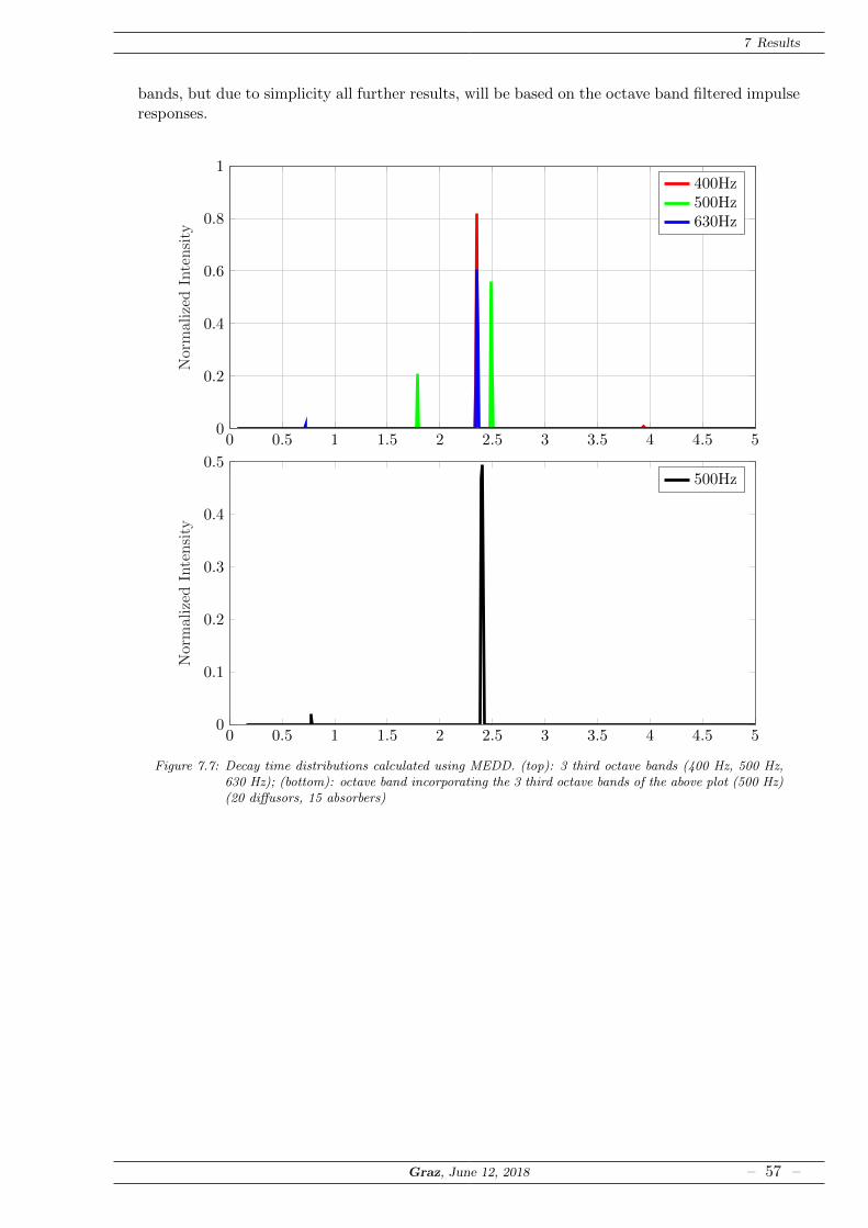
7 Results

bands, but due to simplicity all further results, will be based on the octave band filtered impulseresponses.

0 0.5 1 1.5 2 2.5 3 3.5 4 4.5 50

0.2

0.4

0.6

0.8

1N

orm

aliz

edIn

ten

sity

400Hz500Hz630Hz

0 0.5 1 1.5 2 2.5 3 3.5 4 4.5 50

0.1

0.2

0.3

0.4

0.5

Nor

mal

ized

Inte

nsi

ty

500Hz

Figure 7.7: Decay time distributions calculated using MEDD. (top): 3 third octave bands (400 Hz, 500 Hz,630 Hz); (bottom): octave band incorporating the 3 third octave bands of the above plot (500 Hz)(20 diffusors, 15 absorbers)

Graz, June 12, 2018 – 57 –

7 Results

7.2.2 Number of Absorbers

With the gained possibility to visualize decay time distributions using MEDD, one can now tryto make observations on the behaviour of the multiple sloped effect while changing differentarchitectural parameters in the reverberation chamber. The first investigation of this kind to bemade is the variation of the number of absorbers positioned in the room. The following figuresshow the decay times with intensities greater than one tenth of the maximum of each frequencyband’s decay time distribution. This illustration yields a good comparison of the number ofslopes present in a given measurement.

300 400 500 600 700 800 900 1,000 1,10031

63

125

250

500

1k

2k

4k

8k

Decay Time (ith tau-component)

Fre

qu

ency

Ban

d

Figure 7.8: Detected decay times without corresponding intensities in the reverbeation chamber without dif-fusors and a varying number of absorbing specimen. (red - 0 absorbers, green - 5 absorbers, blue- 15 absorbers)

In figure 7.8, one can find the only single slope in the 1000 Hz band of the measurement withoutany absorber in the room (black). For all other frequency bands of the investigated measure-ments, MEDD obtained a distribution with two or three seperate peaks. This reflects theexpected existance of two or multiple slopes in empty reverberation rooms. In the empty rever-beration chamber, all bounding surfaces are considered lightly damped and therefore a uniformdistribution of absorption is given, which supports the existence of a single exponential decaycurve. Nevertheless, the additional requirement of perfect diffusity can still be violated.The largest shift to the left can be observed in the 250 Hz band. A shift to the left regardinga decay time distribution represents a change towards a shorter decay time which as a resultcan be considered an increase of absorption. In figure 7.8, the increase of absorption is repre-sented by the different measurements with a different number of absorbing specimen placed inthe reverberation chamber. For lower and higher frequencies than the mentioned 250 Hz band,

Graz, June 12, 2018 – 58 –

7 Results

this effect decreases, whereas for the lowest measured frequency band nearly no effect can beobserved. This does underline the low absorption coefficient of thin porous absorbers at lowfrequencies.

300 400 500 600 700 800 900 1,000 1,10031

63

125

250

500

1k

2k

4k

8k

Decay Time (ith tau-component)

Fre

qu

ency

Ban

d

Figure 7.9: Detected decay times without corresponding intensities in the reverberation chamber with 6 dif-fusors and a varying number of absorbing specimen. (red - 0 absorbers, green - 5 absorbers, blue- 15 absorbers)

With the application of diffusors, the diffusity should be increased. Perfect diffusity is oftendescribed as a requirement for obtaining a single exponential decay curve. With only six addi-tional diffusors, the number of single sloped frequency bands increases and now spans a rangefrom 250 Hz to 1000 Hz. This fact only holds for the room without absorbing specimen. Oncean absorber is placed in the room, the diffusity decreases and therefore also the number ofsingle sloped octave bands does. For an accurate calculation of the absorption coefficient in agiven frequency band, both decay time distributions should only contain a single peak, otherwisedifferent calculation methods yet to be developed have to be used. According to [1], the firstslope of a EDC represents the sum of all existing decaying components. With that in mind,the choice of the first non-zero peak of the decay time distribution computed by MEDD as therepresentative when calculating the absorption coefficient would be a possible solution.

Graz, June 12, 2018 – 59 –

7 Results

300 400 500 600 700 800 900 1,000 1,10031

63

125

250

500

1k

2k

4k

8k

Decay Time (ith tau-component)

Fre

qu

ency

Ban

d

Figure 7.10: Detected decay times without corresponding intensities in the reveration chamber with 20 dif-fusors and a varying number of absorbing specimen. (red - 0 absorber, green - 5 absorber, blue- 15 absorber)

The number of diffusors in the room is increased to 20 for the measurement represented in figure7.10 which causes the EDC of the room containing 15 absorbers to start having single slopes.Considering again the calculation of the absorption coefficient with the commonly used method,one would now obtain reasonable results for 2 consecutive frequency bands. As the decay timedistributions have single peaks at 500 Hz and 1000 Hz, the number of absobers, choosing betweenfive or fifteen, has no influence on the validity of the method.

Graz, June 12, 2018 – 60 –

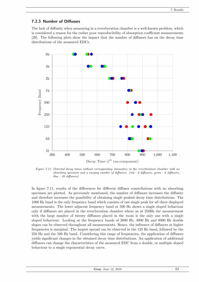
7 Results

7.2.3 Number of Diffusors

The lack of diffusity when measuring in a reverberation chamber is a well-known problem, whichis considered a reason for the rather poor reproducibility of absorption coefficient measurements[29]. The following plots show the impact that the number of diffusors has on the decay timedistributions of the measured EDCs.

300 400 500 600 700 800 900 1,000 1,10031

63

125

250

500

1k

2k

4k

8k

Decay Time (ith tau-component)

Fre

qu

ency

Ban

d

Figure 7.11: Detected decay times without corresponding intensities in the reverberation chamber with noabsorbing specimen and a varying number of diffusors. (red - 0 diffusors, green - 6 diffusors,blue - 20 diffusors)

In figure 7.11, results of the differences for different diffusor constellations with no absorbingspecimen are plotted. As previously mentioned, the number of diffusors increases the diffusityand therefore increases the possibility of obtaining single peaked decay time distributions. The1000 Hz band is the only frequency band which consists of one single peak for all three displayedmeasurements. The lower adjacent frequency band at 500 Hz shows a single sloped behaviouronly if diffusors are placed in the reverberation chamber where as at 250Hz the measurementwith the large number of twenty diffusors placed in the room is the only one with a singlesloped behaviour. Looking at the frequency bands of 2000 Hz, 4000 Hz and 8000 Hz doubleslopes can be observed throughout all measurements. Hence, the influence of diffusors at higherfrequencies is marginal. The largest spread can be observed in the 125 Hz band, followed by the250 Hz and the 500 Hz band. Considering this range of frequencies, the application of diffusorsyields significant changes in the obtained decay time distributions. An application of additionaldiffusors can change the characteristics of the measured EDC from a double, or multiple slopedbehaviour to a single exponential decay curve.

Graz, June 12, 2018 – 61 –

7 Results

300 400 500 600 700 800 900 1,000 1,10031

63

125

250

500

1k

2k

4k

8k

Decay Time (ith tau-component)

Fre

qu

ency

Ban

d

Figure 7.12: Detected decay times without corresponding intensities in the reverberation chamber with 5absorbers and a varying number of diffusors. (red - 0 diffusors, green - 6 diffusors, blue - 20diffusors)

With an increase of the number of absorbers to five the few single slopes observed in figure7.11 vanish, as the diffusity of the soundfield decreases. The differences between the diffusorconstellations are reduced to a time and intensity shift of the two obtained peaks in the decaytime distribution. The left shift previously described as a effect of the added absorption now isa result of the additional diffusors postitioned in the room. The increase of the diffusity of thesound field allows the absorbing surfaces to absorb more sound energy and therefore generate arelatively small left shift in the decay time distribution compared to the left shift created by anadded absorber (see fig. 7.13).

1 1.2 1.4 1.6 1.8 2 2.2 2.4 2.6 2.8 3 3.2 3.4 3.6 3.8 40

0.2

0.4

0.6

0.8

Decay Time (s)

Nor

mal

ized

Inte

nsi

ty 0 diffusors6 diffusors20 diffusors

Figure 7.13: Decay time distribution calculated for the 1000 Hz band for different numbers of diffusors and5 absorbers

Graz, June 12, 2018 – 62 –

7 Results

In figure 7.13 the decay time distribution with an increasing number of diffusors tends towards asingle peak. For the measurement with twenty diffusors placed in the room, the second detecteddecay time corresponds to only one tenth of the primary decay time. The resulting decay curvecan be regarded as close to single sloped.

300 400 500 600 700 800 900 1,000 1,10031

63

125

250

500

1k

2k

4k

8k

Decay Time (ith tau-component)

Fre

qu

ency

Ban

d

Figure 7.14: Detected decay times without corresponding intensities in the reverberation chamber with 15absorbers and a varying number of diffusors. (red - 0 diffusors, green - 6 diffusors, blue - 20diffusors)

With 15 absorbers present, the left shift of the decay time distribution represents the shortenedreverberation time in the room due to the absorbing specimen. Against the expectations, the1000 Hz band now shows single sloped behaviour for 20 diffusors and 15 absorbers.Regarding the three figures visualizing the effect of a different number of diffusors, the leastinfluence on the decay time distributions can be observed for higher frequencies. The largestdeviations for a given absorbing specimen and a variation of the number of diffusors can befound in the 125 Hz band followed by the 250 Hz band.

Graz, June 12, 2018 – 63 –

8Conclusion and Outlook

Investigating new methods of extracting decay times from a given energy decay curve does notonly yield the potential of finding a more accurate solution than the common linear regressionmethod. The presence of multiple sloped decay curves presents a significant problem whenevaluating decay times using the linear regression method. Expanding this method to fitting asum of exponentials to the data offers the possibility of evaluating more than one slope.

VARPROThe adapted version of the VARPRO algorithm offers a time efficient alternative to fitting alinear regression to the data. Previous to triggering the calculation process, the number ofslopes present in the given decay curve has to be entered. This fact and the loss of the ro-bustness for more than one decay component make this algorithm a weak choice. If only oneexponential term is fitted to the data, the solution represents an accurate fit of the first slope.As a result, VARPRO can be used as a tool to compute an estimate for Tearly from a given EDC.

Considering the weaknesses of the VARPRO algorithm, the second adapted algorithm offers thepossibility to fit a sum of exponentials to the data, without the handicap of having to know thenumber of present slopes:

RILTThe RILT algorithm as an emulation of the CONTIN program offers a great tool to obtainthe corresponding intensities for a given decay time grid using a nonlinear least squares fittingapproach. The computation time increases exponentially with the number of grid points whichdecreases its potential when investigating a wider decay time distribution.

Additionally, the obtained intensities as a function of the decay times can be regarded as a decaytime distribution. The last investigated algorithm estimates a decay time distribution using astochastic aproach:

MEDDMEDD represents a program to extract the decay time distribution from a given energy decaycurve. The inverse Laplace transform is estimated by using a quantified maximum entropy ap-proach in the singular value space.MEDD allows the user to select the subprograms needed for the calculation process, to adaptthe user-specified variables and to further shorten the time needed for the computation by us-ing precalculated analysis matrices. The additionally written subprograms m plot and m saveallow one to simultaneously visualize the results to review the obtained solution and to save allparameters needed for a reproduction.

Graz, June 12, 2018 – 64 –

8 Conclusion and Outlook

The results gained using MEDD underline the expectation of the existence of multiple slopeddecay curves in a reverberation chamber. More than one peak in the obtained decay time dis-tributions is visible for most of the investigated datasets.The found new method for extracting decay times from a given measured EDC in room acousticsrepresents a time-efficient tool to evaluate more than a single slope. Furthermore, the resultsobtained by MEDD could be used for the calculation of the absorption coefficient and the de-velopment of a new estimate for the amount of MSE present in an EDC.The frequency range to be used for the calculation of the absorption coefficient using the linearregression method to obtain the reverberation times from two separate reverberation time mea-surements does in none of the cases investigated hold for both the empty and the state with anabsorbing specimen as it needs single slopes to maintain its validity. Using the first peak of thedecay time distribution calculated by MEDD offers a possible alternative, which shows the leastdeviation from the idealised model compared to the other methods tested in [54].

Graz, June 12, 2018 – 65 –

AAppendix

Graz, June 12, 2018 – 66 –

A Appendix

List of Symbols and Abbreviations

φ velocity potential

v velocity

p pressure

ρ= density

k = ωc wave number

c velocity of sound

ω angular frequency

T, T30, T60 reverberation time

∆f 3dB-bandwidth

λ wavelength

A, a, c amplitude

τ, δ, α decay constant

H(δ),Φ(τ) decay time distribution

L Laplace transform

L−1 inverse Laplace transform

W weight vector

η nonlinear model

Φ linear transform kernel

y,D data

N, ν noise

J cost function

R regularization term

α regularization parameter

pr probability

σ variance

Γ Gamma function

L Likelihood function

S Shannon entropy

EDC energy decay curve

VARPRO Variable Projection Algorithm

RILT Regularized Inverse Laplace Transform

MEDD Maximum Entropy Decay time Distribution

MELT Maximum Entropy Lifetime Analysis Tool

DSE double sloped effect

MSE multiple sloped effect, mean squared error

LDT late decay time

EDT early decay time

PDF probability density function

PAD positive additive distribution

DTU Danmarks Tekniske Universitet

SNR Signal to Noise Ratio

Graz, June 12, 2018 – 67 –

A Appendix

Data used for Figures

Figure dataset frequency band [Hz]

6.1 diff20 15abs 2506.2 diff20 15abs 2506.3 diff20 empty 2506.4 diff20 empty 5006.5 diff0 empty 1256.6 diff0 empty 1256.7 diff0 empty 40006.8 diff0 empty 40006.9 diff0 empty 40006.10 diff0 empty 5006.11 diff0 empty 2506.12 diff0 empty 10006.13 diff0 empty 10006.14 diff0 empty 10006.15 diff20 empty 5006.16 diff20 empty 5006.17 diff20 empty 40006.18 diff20 empty 40007.2 diff0 empty 257.3 diff0 empty 257.4 diff0 empty 257.5 diff20 empty oct7.6 diff20 15abs 2507.7 diff20 15abs 5007.8 diff0 empty, diff0 5abs, diff0 15abs oct7.9 diff6 empty, diff6 5abs, diff6 15abs oct7.10 diff20 empty, diff20 5abs, diff20 15abs oct7.11 diff0 empty, diff6 empty, diff20 empty oct7.12 diff0 5abs, diff6 5abs, diff20 5abs oct7.14 diff0 15abs, diff6 15abs, diff20 15abs oct7.13 diff0 15abs, diff6 15abs, diff20 15abs 1000

Graz, June 12, 2018 – 68 –

List of Figures

2.1 Rectangular room in a Cartesian coordinate system [9] . . . . . . . . . . . . . . . 62.2 Sound pressure distribution of the 0-2-0 axial mode in a room . . . . . . . . . . . 62.3 Overview of existing normal modes illustrated in the frequency space [9] . . . . . 72.4 RIR measurement in Philharmonic Hall, New York (Octobre 19, 1963). Noise

source near center stage, receiving point on Second Terrace. Omnidirectionalmicrophone and loudspeaker. [14] . . . . . . . . . . . . . . . . . . . . . . . . . . . 10

2.5 Graphical Representation of the calculation of to different MSE estimates, T30/T15

and LDT/EDT . . . . . . . . . . . . . . . . . . . . . . . . . . . . . . . . . . . . . 112.6 Results for the absorption coefficient α from a round robin test performed in 19

different laboratories with 3 different absorbing specimen [28] . . . . . . . . . . . 122.7 Visualisation of an EDC and a single exponential fit summed with the estimated

noisefloor plotted logarithmically for the 250 Hz octave band (top) and the 4000Hz octave band (bottom) . . . . . . . . . . . . . . . . . . . . . . . . . . . . . . . 13

2.8 Common distributions with the corresponding calculated decay curves [1] . . . . 142.9 Illustration of the calculation of the methods (1) and (2) [31] . . . . . . . . . . . 162.10 Illustration of the calculation of the methods (3) and (4) [31] . . . . . . . . . . . 172.11 Comparison of the EDC calculated using method (1) and method (5) . . . . . . . 17

3.1 Probability density function of the χ2k-distribution . . . . . . . . . . . . . . . . . 25

4.1 Flow graph of the MEDD program using either medd or medd loop as the mainprogram . . . . . . . . . . . . . . . . . . . . . . . . . . . . . . . . . . . . . . . . 27

4.2 Visualisation of a anaylsis matrix T . . . . . . . . . . . . . . . . . . . . . . . . . 294.3 Figures plotted when using m plot for the visualisation of the results obtained by

MEDD . . . . . . . . . . . . . . . . . . . . . . . . . . . . . . . . . . . . . . . . . . 31

5.1 Floor plan of the reverberation room with all receiver and source positions markedand an exemplaric absorber setup . . . . . . . . . . . . . . . . . . . . . . . . . . . 32

5.2 Picture of the measurement setup with 5 and 15 absorbers introduced . . . . . . 33

6.1 Single slope estimation for a double sloped EDC using VARPRO with an auto-mated noisefloor estimation (20 diffusors, 15 absorbers, 250 Hz octave band) . . 36

6.2 Single slope estimation for a double sloped EDC using VARPRO with an auto-mated noise subtraction (20 diffusors, 15 absorbers, 250 Hz octave band) . . . . . 36

6.3 Double slope estimation of single sloped data using VARPRO with an automatednoisefloor estimation (20 diffusors, 0 absorbers, 250 Hz octave band) . . . . . . . 37

6.4 Double slope estimation of double sloped data using VARPRO with an automatednoisefloor estimation (20 diffusors, 0 absorbers, 500 Hz octave band) . . . . . . . 37

6.5 Double slope estimation of double sloped data using VARPRO with an automatednoisefloor estimation starting at -5dB (0 diffusors, 0 absorbers, 125 Hz octave band) 38

6.6 Double slope estimation of double sloped data using VARPRO with an automatednoisefloor (0 diffusors, 0 absorbers, 125 Hz octave band) . . . . . . . . . . . . . . 38

6.7 Double slope estimation of double sloped data using VARPRO with an automatednoisefloor (0 diffusors, 0 absorbers, 500 Hz octave band) . . . . . . . . . . . . . . 39

6.8 Plots illustrating the results generated by RILT when investigating a given EDC(0 diffusors, 0 absorbers, 4000 Hz octave band) . . . . . . . . . . . . . . . . . . . 40

6.9 Resulting decay time distribution when using RILT for the same data set as infigure 6.8 with a finer linear grid (0 diffusors, 0 absorbers, 4000 Hz octave band) 41

Graz, June 12, 2018 – 69 –

List of Figures

6.10 Computed decay time distribution for different values of the regularization pa-rameter α using RILT (0 diffusors, 0 absorbers, 500 Hz octave band) . . . . . . . 41

6.11 Using RILT with different downsampling ratios (0 diffusors, 0 absorbers, 250 Hzoctave band) . . . . . . . . . . . . . . . . . . . . . . . . . . . . . . . . . . . . . . 42

6.12 Illustration of the effect of varying the user specified variableNtau on the resultingdecay time distribution for a double sloped EDC (0 diffusors, 0 absorbers, 1000Hz octave band) . . . . . . . . . . . . . . . . . . . . . . . . . . . . . . . . . . . . 44

6.13 Illustration of the effect of varying the user specified variable increment on the re-sulting decay time distribution for a double sloped EDC (0 diffusors, 0 absorbers,1000 Hz octave band) . . . . . . . . . . . . . . . . . . . . . . . . . . . . . . . . . 44

6.14 Illustration to correctly choose the values for endwgthstart and endwgthstop (0diffusors, 0 absorbers, 1000 Hz octave band) . . . . . . . . . . . . . . . . . . . . . 45

6.15 Decay time distributions calculated by RILT and MEDD for a single sloped EDC(20 diffusors, 0 absorbers, 500 Hz octave band) . . . . . . . . . . . . . . . . . . . 46

6.16 Illustration of estimates and residuals for a given measured EDC. Estimates arecalculated by using the maximum of each decay time distribution (RILT, MEDD)to create a single exponential decay curve added to the estimated noise floor. (20diffusors, 0 absorbers, 500 Hz octave band) . . . . . . . . . . . . . . . . . . . . . 47

6.17 Decay time distributions calculated by RILT and MEDD for a double sloped EDC(20 diffusors, 0 absorbers, 4000 Hz octave band) . . . . . . . . . . . . . . . . . . 48

6.18 Illustration of estimates and residuals to a given EDC. Estimates are calculatedby using the maxima of the selected peaks from each decay time distribution(RILT, MEDD) to create a multi (double) exponential decay curve added to theestimated remaining noise floor. (20 diffusors, 0 absorbers, 4000 Hz octave band) 49

7.1 Absolute sound pressure distribution for the 0-1-0 axial mode . . . . . . . . . . . 507.2 EDCs of each measurement position. (top): all 12 receiver-source combinations;

(bottom): averaged source positions (0 diffusors, 0 absorbers, 25 Hz third octaveband) . . . . . . . . . . . . . . . . . . . . . . . . . . . . . . . . . . . . . . . . . . 51

7.3 Different averaged EDCs considering a neglection of measurement positions M1and M4 (0 diffusors, 0 absorbers, 25 Hz third octave band) . . . . . . . . . . . . 52

7.4 top: EDC of M2 (averaged source positions); bottom: EDC of M3 (averagedsource positions) (0 diffusors, 0 absorbers, 25 Hz third octave band) . . . . . . . 52

7.5 3D plot of the decay time distributions in octave bands calculated by MEDD (20diffusors, 0 absorbers, octave bands) . . . . . . . . . . . . . . . . . . . . . . . . . 54

7.6 Decay time distributions calculated using MEDD. (top): 3 third octave bands(200 Hz, 250 Hz, 315 Hz); (bottom): octave band incorporating the 3 thirdoctave bands of the above plot (250 Hz) (20 diffusors, 15 absorbers) . . . . . . . 56

7.7 Decay time distributions calculated using MEDD. (top): 3 third octave bands(400 Hz, 500 Hz, 630 Hz); (bottom): octave band incorporating the 3 thirdoctave bands of the above plot (500 Hz) (20 diffusors, 15 absorbers) . . . . . . . 57

7.8 Detected decay times without corresponding intensities in the reverbeation cham-ber without diffusors and a varying number of absorbing specimen. (red - 0absorbers, green - 5 absorbers, blue - 15 absorbers) . . . . . . . . . . . . . . . . . 58

7.9 Detected decay times without corresponding intensities in the reverberation cham-ber with 6 diffusors and a varying number of absorbing specimen. (red - 0 ab-sorbers, green - 5 absorbers, blue - 15 absorbers) . . . . . . . . . . . . . . . . . . 59

7.10 Detected decay times without corresponding intensities in the reveration chamberwith 20 diffusors and a varying number of absorbing specimen. (red - 0 absorber,green - 5 absorber, blue - 15 absorber) . . . . . . . . . . . . . . . . . . . . . . . . 60

Graz, June 12, 2018 – 70 –

List of Figures

7.11 Detected decay times without corresponding intensities in the reverberation cham-ber with no absorbing specimen and a varying number of diffusors. (red - 0diffusors, green - 6 diffusors, blue - 20 diffusors) . . . . . . . . . . . . . . . . . . . 61

7.12 Detected decay times without corresponding intensities in the reverberation cham-ber with 5 absorbers and a varying number of diffusors. (red - 0 diffusors, green- 6 diffusors, blue - 20 diffusors) . . . . . . . . . . . . . . . . . . . . . . . . . . . . 62

7.13 Decay time distribution calculated for the 1000 Hz band for different numbers ofdiffusors and 5 absorbers . . . . . . . . . . . . . . . . . . . . . . . . . . . . . . . . 62

7.14 Detected decay times without corresponding intensities in the reverberation cham-ber with 15 absorbers and a varying number of diffusors. (red - 0 diffusors, green- 6 diffusors, blue - 20 diffusors) . . . . . . . . . . . . . . . . . . . . . . . . . . . . 63

Graz, June 12, 2018 – 71 –

List of Tables

5.1 Nomenclature for the stored matrices containing the EDCs for each frequencyband (octaves) . . . . . . . . . . . . . . . . . . . . . . . . . . . . . . . . . . . . . 34

5.2 Nomenclature for the stored matrices containing the EDCs for each frequencyband (third-octaves) . . . . . . . . . . . . . . . . . . . . . . . . . . . . . . . . . . 34

6.1 Decay times calculated by VAPRO and MEDD . . . . . . . . . . . . . . . . . . . 436.2 Reverberation times and corresponding intensities for the selected peaks in each

algorithm’s solution for the double sloped EDC (see fig 6.17) . . . . . . . . . . . 486.3 Mean squared error between the generated estimates and the actual EDC . . . . 48

A.1 Characteristics of the used octave and third octave bands . . . . . . . . . . . . . 74

Graz, June 12, 2018 – 72 –

List of Tables

List of Matlab Scripts

VARPRO

varpro.m Separable nonlinear least squares solver by O’Leary [34]

adaex.m Calculates the derivative of the multi-exponential model (called during varpro.m)

varpro decaycurves noisecalc.m Excitation of the varpro algorithm including a noise floor esti-mation

varpro decaycurves noisecalc.m Excitation of the varpro algorithm including a noise floor esti-mation

RILT

rilt rt.m Adapted version of the RILT algorithm

rilt decaycuves.m Excitation of the rilt rt program

MEDD

medd.m Main program of MEDD

m input.m Only file to be adapted by the user (user input)

m data.m Loads and prepares the data for the further calculation

m tcmat.m Calculates the analysis matrix T

m pre.m Prefiltering process using a general linear filter

m iter.m Quantified entropy maximisation using the algorithm by Bryan [8]

m res.m Preparation of the results

m save.m Saving all needed paramters for the reproduction

m plot.m Visualising the iteration process and solution

MEDD loop 3

medd loop3.m Excites MEDD in a loop to investigate the EDC’s of each third octave band ina row

stem 3.m Script to create stem3 plots of the variation of absorbers or diffusors in third octavebands

MEDD loop 8

medd loop8.m Excites MEDD in a loop to investigate the EDC’s of each octave band in a row

stem 8.m Script to create stem3 plots of the variation of absorbers or diffusors in third octavebands

Graz, June 12, 2018 – 73 –

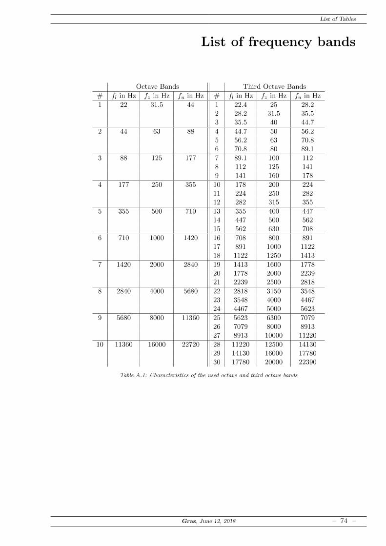
List of Tables

List of frequency bands

Octave Bands Third Octave Bands

# fl in Hz fz in Hz fu in Hz # fl in Hz fz in Hz fu in Hz

1 22 31.5 44 1 22.4 25 28.22 28.2 31.5 35.53 35.5 40 44.7

2 44 63 88 4 44.7 50 56.25 56.2 63 70.86 70.8 80 89.1

3 88 125 177 7 89.1 100 1128 112 125 1419 141 160 178

4 177 250 355 10 178 200 22411 224 250 28212 282 315 355

5 355 500 710 13 355 400 44714 447 500 56215 562 630 708

6 710 1000 1420 16 708 800 89117 891 1000 112218 1122 1250 1413

7 1420 2000 2840 19 1413 1600 177820 1778 2000 223921 2239 2500 2818

8 2840 4000 5680 22 2818 3150 354823 3548 4000 446724 4467 5000 5623

9 5680 8000 11360 25 5623 6300 707926 7079 8000 891327 8913 10000 11220

10 11360 16000 22720 28 11220 12500 1413029 14130 16000 1778030 17780 20000 22390

Table A.1: Characteristics of the used octave and third octave bands

Graz, June 12, 2018 – 74 –

Bibliography

[1] H. Kuttruff, “Eigenschaften und Auswertung von Nachhallkurven,” Acta Acustica unitedwith Acustica, vol. 8, no. 4, pp. 273–280, 1958.

[2] F. Jacobsen and P. M. Juhl, Fundamentals of general linear acoustics. John Wiley & Sons,2013.

[3] F. Jacobsen, “The sound field in a reverberation room,” Technical University of Denmark,Lyngby, Denmark, 2011.

[4] N. Xiang, P. Goggans, T. Jasa, and P. Robinson, “Bayesian characterization of multiple-slope sound energy decays in coupled-volume systems,” The Journal of the Acoustical So-ciety of America, vol. 129, no. 2, pp. 741–752, 2011.

[5] L. Hoffmann, A. Shukla, M. Peter, B. Barbiellini, and A. Manuel, “Linear and non-linearapproaches to solve the inverse problem: applications to positron annihilation experiments,”Nuclear Instruments and Methods in Physics Research Section A: Accelerators, Spectrom-eters, Detectors and Associated Equipment, vol. 335, no. 1-2, pp. 276–287, 1993.

[6] A. Shukla, L. Hoffmann, A. A. Manuel, and M. Peter, “Melt 4.0 a program for positronlifetime analysis,” in Materials Science Forum, vol. 255. Trans Tech Publ, 1997, pp.233–237.

[7] R. Bryan, “Maximum entropy analysis of oversampled data problems,” European BiophysicsJournal, vol. 18, no. 3, pp. 165–174, 1990.

[8] ——, “Solving oversampled data problems by maximum entropy,” in Maximum Entropyand Bayesian Methods. Springer, 1990, pp. 221–232.

[9] E. Meyer, Physical and applied acoustics: an introduction. Elsevier, 2012.

[10] P. E. Sabine, “What is measured in sound absorption measurements,” The Journal of theAcoustical Society of America, vol. 6, no. 4, pp. 239–245, 1935.

[11] M. R. Schroeder, “The ‘‘Schroeder frequency’’revisited,” The Journal of the AcousticalSociety of America, vol. 99, no. 5, pp. 3240–3241, 1996.

[12] F. Jacobsen, The diffuse sound field: Statistical considerations concerning the reverberantfield in the steady state. Acoustics Laboratory, Technical University of Denmark, 1979.

[13] M. Nolan, J. L. Davy, and J. Brunskog, “Estimating the diffuseness of sound fields: Awavenumber analysis method,” The Journal of the Acoustical Society of America, vol. 141,no. 5, pp. 3784–3784, 2017.

[14] M. R. Schroeder, “Response to “Comments on ‘New Method of Measuring ReverberationTime’”[PW Smith, Jr., J. Acoust. Soc. Am. 38, 359 (L)(1965)],” The Journal of the Acous-tical Society of America, vol. 38, no. 2, pp. 359–361, 1965.

[15] F. Hunt, L. Beranek, and D.-Y. Maa, “Analysis of sound decay in rectangular rooms,” TheJournal of the Acoustical Society of America, vol. 11, no. 1, pp. 80–94, 1939.

[16] E. Nilsson, “Decay processes in rooms with non-diffuse sound fields Part I: Ceiling treatmentwith absorbing material,” Building Acoustics, vol. 11, no. 1, pp. 39–60, 2004.

[17] ——, “Decay processes in rooms with non-diffuse sound fields. Part II: Effect of irregulari-ties,” Building Acoustics, vol. 11, no. 2, pp. 133–143, 2004.

Graz, June 12, 2018 – 75 –

Bibliography

[18] D. T. Bradley and L. M. Wang, “Optimum absorption and aperture parameters for realis-tic coupled volume spaces determined from computational analysis and subjective testingresults,” The Journal of the Acoustical Society of America, vol. 127, no. 1, pp. 223–232,2010.

[19] ——, “Quantifying the double slope effect in coupled volume room systems,” BuildingAcoustics, vol. 16, no. 2, pp. 105–123, 2009.

[20] N. Xiang, “Evaluation of reverberation times using a nonlinear regression approach,” TheJournal of the Acoustical Society of America, vol. 98, no. 4, pp. 2112–2121, 1995.

[21] N. Xiang and P. M. Goggans, “Evaluation of decay times in coupled spaces: Bayesianparameter estimation,” The Journal of the Acoustical Society of America, vol. 110, no. 3,pp. 1415–1424, 2001.

[22] N. Xiang, P. M. Goggans, T. Jasa, and M. Kleiner, “Evaluation of decay times in cou-pled spaces: Reliability analysis of Bayeisan decay time estimation,” The Journal of theAcoustical Society of America, vol. 117, no. 6, pp. 3707–3715, 2005.

[23] N. Xiang, Y. Jing, and A. C. Bockman, “Investigation of acoustically coupled enclosuresusing a diffusion-equation model,” The Journal of the Acoustical Society of America, vol.126, no. 3, pp. 1187–1198, 2009.

[24] T. Jasa and N. Xiang, “Efficient estimation of decay parameters in acoustically coupled-spaces using slice sampling,” The Journal of the Acoustical Society of America, vol. 126,no. 3, pp. 1269–1279, 2009.

[25] N. Xiang and C. Fackler, “Objective Bayesian analysis in acoustics,” Acoust. Today, vol. 11,no. 2, pp. 54–61, 2015.

[26] A. Cops, J. Vanhaecht, and K. Leppens, “Sound absorption in a reverberation room: Causesof discrepancies on measurement results,” Applied Acoustics, vol. 46, no. 3, pp. 215–232,1995.

[27] K. V. Horoshenkov, A. Khan, F.-X. Becot, L. Jaouen, F. Sgard, A. Renault, N. Amirouche,F. Pompoli, N. Prodi, P. Bonfiglio et al., “Reproducibility experiments on measuring acous-tical properties of rigid-frame porous media (round-robin tests),” The Journal of the Acous-tical Society of America, vol. 122, no. 1, pp. 345–353, 2007.

[28] A.-C. Thysell, “Test Codes for Suspended Ceilings,” Tyrens AB, 06 2011.

[29] M. Vercammen, “Improving the accuracy of sound absorption measurement according toISO 354,” in Proceedings of the International Symposium on Room Acoustics. MelbourneAustralia, 2010.

[30] E. DIN, “3382: Akustik–Messung der Nachhallzeit von Raumen mit Hinweis auf andereakustische Parameter,” ISO, vol. 3382, no. 1997, p. 03, 2000.

[31] M. Guski and M. Vorlander, “Noise compensation methods for room acoustical parameterevaluation,” in International Symposium on Room Acoustics, 2013.

[32] A. Lundeby, T. E. Vigran, H. Bietz, and M. Vorlander, “Uncertainties of measurements inroom acoustics,” Acta Acustica united with Acustica, vol. 81, no. 4, pp. 344–355, 1995.

[33] W. T. Chu, “Comparison of reverberation measurements using Schroeder’s impulse methodand decay-curve averaging method,” The Journal of the Acoustical Society of America,vol. 63, no. 5, pp. 1444–1450, 1978.

Graz, June 12, 2018 – 76 –

Bibliography

[34] D. P. O’leary and B. W. Rust, “Variable projection for nonlinear least squares problems,”Computational Optimization and Applications, vol. 54, no. 3, pp. 579–593, 2013.

[35] G. H. Golub and V. Pereyra, “The differentiation of pseudo-inverses and nonlinear leastsquares problems whose variables separate,” SIAM Journal on Numerical Analysis, vol. 10,no. 2, pp. 413–432, 1973.

[36] G. Golub and V. Pereyra, “Separable nonlinear least squares: the variable projectionmethod and its applications,” Inverse problems, vol. 19, no. 2, p. R1, 2003.

[37] V. Pereyra and G. Scherer, Exponential data fitting and its applications. Bentham SciencePublishers, 2010.

[38] L. Kaufman, “A variable projection method for solving separable nonlinear least squaresproblems,” BIT Numerical Mathematics, vol. 15, no. 1, pp. 49–57, 1975.

[39] A. Ruhe and P. A. Wedin, “Algorithms for separable nonlinear least squares problems,”SIAM review, vol. 22, no. 3, pp. 318–337, 1980.

[40] J. Bolstad, “Varpro package,” Computer SCience Opt. Stanford Univ, 1977.

[41] “RILT - Regularized Inverse Laplace Transform,” https://de.mathworks.com/matlabcentral/fileexchange/6523-rilt, accessed: 2018-03-28.

[42] S. W. Provencher, “CONTIN: a general purpose constrained regularization program for in-verting noisy linear algebraic and integral equations,” Computer Physics Communications,vol. 27, no. 3, pp. 229–242, 1982.

[43] S. Provencher, “A Fourier method for the analysis of exponential decay curves,” Biophysicaljournal, vol. 16, no. 1, pp. 27–41, 1976.

[44] ——, “An eigenfunction expansion method for the analysis of exponential decay curves,”The Journal of Chemical Physics, vol. 64, no. 7, pp. 2772–2777, 1976.

[45] S. W. Provencher and V. G. Dovi, “Direct analysis of continuous relaxation spectra,” Jour-nal of biochemical and biophysical methods, vol. 1, no. 6, pp. 313–318, 1979.

[46] S. W. Provencher and R. H. Vogel, “Information loss with transform methods in systemidentification: a new set of transforms with high information content,” Mathematical Bio-sciences, vol. 50, no. 3-4, pp. 251–262, 1980.

[47] S. W. Provencher, “A constrained regularization method for inverting data represented bylinear algebraic or integral equations,” Computer Physics Communications, vol. 27, no. 3,pp. 213–227, 1982.

[48] ——, Contin (Version 2) users manual. EMBL, 1984.

[49] A. N. Tikhonov, V. A. Arsenin, and V. Kotliar, “Methodes de resolution de problemes malposes,” 1976.

[50] J. Skilling, “Quantified maximum entropy,” in Maximum Entropy and Bayesian Methods.Springer, 1990, pp. 341–350.

[51] G. Osius, “Exkurse zur Wahrscheinlichkeitstheorie, Linearen Algebra etc. zusammengestelltfur die Veranstaltung Lineare Modelle in der Statistik,” url = http://www.math.uni-bremen.de/osius/download/lehre/Skripte/LM/Osius-LineareModelle-Exkurse 2010-07.pdf, Jul. 2010.

Graz, June 12, 2018 – 77 –

Bibliography

[52] E. ISO, “354,” Acoustics-Measurement of sound absorption in a reverberation room, 2003.

[53] G. Dlubek, C. Hubner, and S. Eichler, “Do the CONTIN or the MELT programs accuratelyreveal the o-Ps lifetime distribution in polymers? Analysis of experimental lifetime spectraof amorphous polymers, journal = Nuclear Instruments and Methods in Physics ResearchSection B: Beam Interactions with Materials and Atoms,” vol. 142, no. 1-2, pp. 191–202,1998.

[54] J. Balint, F. Muralter, M. Nolan, and C.-H. Jeong, “Energy decay curves in reverberationchambers and the influence of scattering objects on the absorption coefficient of a sample,”in Euronoise 2018 Crete. European Acoustics Association, 2018.

Graz, June 12, 2018 – 78 –