Embed Size (px)
Citation preview

Newtonian Versus Relativistic Cosmology
Master Thesis
by
Samuel Flender
1st corrector: Prof. Dr. Dominik Schwarz
2nd corrector: Prof. Dr. Dietrich Bödeker
University of Bielefeld
January 2012

Contents
1 Introduction 4
2 The homogeneous and isotropic universe 6
2.1 Basic equations . . . . . . . . . . . . . . . . . . . . . . . . . . . . . . . . . . . . . . . . . 6
2.2 Content of the universe . . . . . . . . . . . . . . . . . . . . . . . . . . . . . . . . . . . . 7
2.3 Ination . . . . . . . . . . . . . . . . . . . . . . . . . . . . . . . . . . . . . . . . . . . . . 8
2.4 Evolution of scales . . . . . . . . . . . . . . . . . . . . . . . . . . . . . . . . . . . . . . . 10
3 The perturbed universe: Newtonian treatment 12
3.1 Denitions . . . . . . . . . . . . . . . . . . . . . . . . . . . . . . . . . . . . . . . . . . . . 12
3.2 Perturbed elds . . . . . . . . . . . . . . . . . . . . . . . . . . . . . . . . . . . . . . . . . 12
3.3 Perturbed Newtonian equations . . . . . . . . . . . . . . . . . . . . . . . . . . . . . . . . 13
3.3.1 Continuity equation . . . . . . . . . . . . . . . . . . . . . . . . . . . . . . . . . . 13
3.3.2 Poisson equation . . . . . . . . . . . . . . . . . . . . . . . . . . . . . . . . . . . . 14
3.3.3 Euler equation . . . . . . . . . . . . . . . . . . . . . . . . . . . . . . . . . . . . . 15
3.3.4 Summary . . . . . . . . . . . . . . . . . . . . . . . . . . . . . . . . . . . . . . . . 17
3.4 Solutions . . . . . . . . . . . . . . . . . . . . . . . . . . . . . . . . . . . . . . . . . . . . 17
3.4.1 First order solutions . . . . . . . . . . . . . . . . . . . . . . . . . . . . . . . . . . 17
3.4.2 Initial conditions . . . . . . . . . . . . . . . . . . . . . . . . . . . . . . . . . . . . 19
3.4.3 Transfer function . . . . . . . . . . . . . . . . . . . . . . . . . . . . . . . . . . . . 20
3.4.4 Second order solutions . . . . . . . . . . . . . . . . . . . . . . . . . . . . . . . . . 24
3.4.5 Discussion . . . . . . . . . . . . . . . . . . . . . . . . . . . . . . . . . . . . . . . . 28
3.4.6 Solutions during Λ-domination . . . . . . . . . . . . . . . . . . . . . . . . . . . . 31
3.5 Newtonian cosmological simulations . . . . . . . . . . . . . . . . . . . . . . . . . . . . . 31
4 The perturbed universe: relativistic treatment 32
4.1 The perturbed metric . . . . . . . . . . . . . . . . . . . . . . . . . . . . . . . . . . . . . 32
4.2 Gauge transformations . . . . . . . . . . . . . . . . . . . . . . . . . . . . . . . . . . . . . 33
4.2.1 Gauge transformations of scalars, vectors and tensors . . . . . . . . . . . . . . . 35
4.2.2 Gauge transformation of metric perturbations . . . . . . . . . . . . . . . . . . . . 36
4.2.3 Gauge transformations of velocity and density perturbations . . . . . . . . . . . 37
4.2.4 Gauge-invariant quantities . . . . . . . . . . . . . . . . . . . . . . . . . . . . . . . 38
4.2.5 Gauges . . . . . . . . . . . . . . . . . . . . . . . . . . . . . . . . . . . . . . . . . 39
4.3 Relativistic equations in the conformal Newtonian gauge . . . . . . . . . . . . . . . . . . 42
4.4 Solutions . . . . . . . . . . . . . . . . . . . . . . . . . . . . . . . . . . . . . . . . . . . . 44
4.4.1 Solutions in the conformal Newtonian gauge . . . . . . . . . . . . . . . . . . . . . 44
4.4.2 Solutions in other gauges . . . . . . . . . . . . . . . . . . . . . . . . . . . . . . . 45
4.4.3 Gauge-invariant solutions . . . . . . . . . . . . . . . . . . . . . . . . . . . . . . . 46
4.5 Vector and tensor perturbations . . . . . . . . . . . . . . . . . . . . . . . . . . . . . . . . 48
2

5 Quantication of relativistic corrections 49
5.1 Relativistic corrections to Newtonian simulations . . . . . . . . . . . . . . . . . . . . . . 49
5.2 Relativistic corrections to the observed power spectrum . . . . . . . . . . . . . . . . . . 51
5.3 Relativistic corrections in ΛCDM models . . . . . . . . . . . . . . . . . . . . . . . . . . . 52
6 Summary and outlook 57
Appendix 58
Appendix A: Helmholtz decomposition theorem . . . . . . . . . . . . . . . . . . . . . . . . . . 58
Appendix B: Statistical properties of Gaussian perturbations . . . . . . . . . . . . . . . . . . 60
Appendix C: Perturbations in the inaton eld . . . . . . . . . . . . . . . . . . . . . . . . . . 62
Appendix D: Meszaros equation . . . . . . . . . . . . . . . . . . . . . . . . . . . . . . . . . . . 63
Appendix E: Identity of synchronous and comoving gauge . . . . . . . . . . . . . . . . . . . . 64
References 66
Acknowledgments 68
3
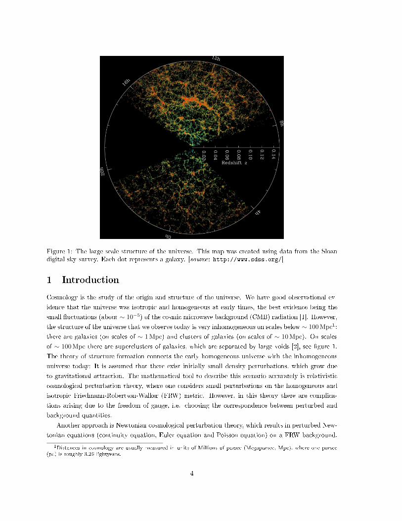
Figure 1: The large scale structure of the universe. This map was created using data from the Sloandigital sky survey. Each dot represents a galaxy. [source: http://www.sdss.org/]
1 Introduction
Cosmology is the study of the origin and structure of the universe. We have good observational ev-
idence that the universe was isotropic and homogeneous at early times, the best evidence being the
small uctuations (about ∼ 10−5) of the cosmic microwave background (CMB) radiation [1]. However,
the structure of the universe that we observe today is very inhomogeneous on scales below ∼ 100 Mpc1:
there are galaxies (on scales of ∼ 1 Mpc) and clusters of galaxies (on scales of ∼ 10 Mpc). On scales
of ∼ 100 Mpc there are superclusters of galaxies, which are separated by large voids [2], see gure 1.
The theory of structure formation connects the early homogeneous universe with the inhomogeneous
universe today: It is assumed that there exist initially small density perturbations, which grow due
to gravitational attraction. The mathematical tool to describe this scenario accurately is relativistic
cosmological perturbation theory, where one considers small perturbations on the homogeneous and
isotropic Friedmann-Robertson-Walker (FRW) metric. However, in this theory there are complica-
tions arising due to the freedom of gauge, i.e. choosing the correspondence between perturbed and
background quantities.
Another approach is Newtonian cosmological perturbation theory, which results in perturbed New-
tonian equations (continuity equation, Euler equation and Poisson equation) on a FRW background.
1Distances in cosmology are usually measured in units of Millions of parsec (Megaparsec, Mpc), where one parsec(pc) is roughly 3.26 lightyears.
4

Figure 2: Result of the Millennium simulation. [source: http://www.mpa-garching.mpg.de]
One has to keep in mind that Newtonian theory is wrong in that it assumes instantaneous gravita-
tional interaction and innite speed of light. However, it turns out that Newtonian and relativistic
cosmological perturbation theory coincide for scales much smaller than the Hubble horizon, which is
basically the size of the observable universe.
Cosmological N -body simulations use Newtonian cosmology to move particles and simulate the
density growth in the universe. These simulations can be used to test our understanding of structure
formation. A famous simulation is the Millennium run (see gure 2), which simulated the behaviour
of ∼ 1010 particles (each particle representing a dark matter clump with a mass of 109 suns) in a
box of ∼ 1Gpc side length [3]. But the question is, how reliable are these simulations, since they use
Newtonian rather than relativistic equations. In this work, we want to study the relativistic corrections
to the Newtonian equations. Cosmological perturbation theory is a major tool to do this.
The outline is as follows: In part 2, we will summarize our current understanding of the universe
and give the most important equations describing it. In part 3, we are going to consider Newtonian
perturbation theory on an expanding FRW background. We will derive and solve the perturbed New-
tonian equations up to second order. In part 4, we will introduce relativistic cosmological perturbation
theory and derive and solve the relativistic evolution equations for the perturbation variables. In part
5, we will quantify the relativistic corrections to cosmological simulations and the observed matter
power spectrum.
5

2 The homogeneous and isotropic universe
2.1 Basic equations
This section resumes the basic equations in cosmology. For a reference, see e.g. [4, 5]. We set c = 1.
The Friedmann equation relates the Hubble parameter to the content of the universe:
H2 =8πG
3ρ(t)− k
a2, (2.1)
where a is the scale factor, H ≡ 1a∂a∂t = a
a is the Hubble parameter, k is the curvature of the universe
and ρ(t) is its energy density. This can consist of matter density, radiation density, or something else.
Dene the critical energy density
ρc ≡3H2
8πG(2.2)
and the relative energy density
Ω(t) ≡ ρ(t)
ρc(t). (2.3)
Then we can rewrite the Friedmann equation as
1− Ω(t) = − k
a2H2. (2.4)
From this equation it can be seen that the universe has critical energy density (Ω = 1) if and only if
the curvature k vanishes. Furthermore, an overcritical universe (Ω > 1) has positive curvature and an
undercritical universe (Ω < 1) has negative curvature.
The equation of state connects the energy density of a given source of energy and the pressure P
that is created by it,
P = wρ, (2.5)
where w is the equation of state parameter.
Another important equation is the continuity equation, which tells how much the energy density
will change in time,
ρ+ 3H(ρ+ P ) = 0. (2.6)
Inserting the equation of state, we nd
ρ+ 3Hρ(1 + w) = 0, (2.7)
which has the solution
ρ = ρ0a−3(1+w), (2.8)
where ρ0 = ρ(t0) is the energy density today (we scale a such that a(t0) = 1). For a spatially at
single uid universe, the Friedmann equation then becomes
a2 =8πG
3ρ0a−(1+3w). (2.9)
6

Figure 3: Content of the universe today. [source: map.gsfc.nasa.gov/universe/uni_matter.html]
Given an equation of state parameter w we can solve this dierential equation for the scale factor a(t).
Finally, we introduce the Raychaudhuri equation, which can be derived from the Friedmann equation
and the continuity equation. It gives the acceleration of the scale factor in terms of energy density and
pressure,a
a= −4πG
3(ρ+ 3P ). (2.10)
2.2 Content of the universe
Now we discuss the dierent components of our universe. The universe contains:
• Matter. This is to a small part (Ωb,0 ' 0.05) baryonic matter, which is mostly hydrogen.
Everything that we see, stars, galaxies and clusters of galaxies, but also interstellar dust is
contained in this number. However, various observations suggest that there is another type of
matter that we cannot see directly, but its gravitational eects [6]. We call this type of matter
dark matter. Matter density ρm, dened as mass per volume, scales as ρm(t) ∼ a−3, because
volume scales as a3. Thus, the equation of state parameter is wm = 0. In other words, matter
does not create any pressure. Today, baryonic and dark matter together make up a relative
energy density of Ωm,0 ' 0.28, but the biggest part of it comes from dark matter, Ωdm,0 ' 0.23.
• Radiation. Radiation density scales as ργ ∼ a−4, because the number density of photons scales
as nγ ∼ a−3 and the energy of each photon scales as Eγ ∼ 1λ ∼ a−1. Hence, the equation of
state parameter is wγ = 13 . Measurements show that today Ωγ,0 ' 10−4, which comes mainly
from CMB (cosmic microwave background) photons.
• Curvature. It is not known for sure if the universe is spatially at. If curvature exists, then it acts
eectively as an energy density, as can be seen from the Friedmann equation, with ρk ∼ a−2, so
that wk = − 13 . However, measurements show that the eect of curvature cannot be large today,
|Ωk,0| . 10−2.
7
~a−4
m~a−3
=const
a
todayradiation domination matter domination dark energy domination
Figure 4: Overview over the dierent epochs of our universe (in a logarithmic scaling). Becauseradiation, matter and dark energy density scale dierently with time, there exist eras where one ofthem is dominating.
• Λ. Dark energy (also called vacuum energy or cosmological constant Λ) is a component of the
universe whose energy density does not change with time. Consequently, the equation of state
parameter is wΛ = −1, whence it creates negative pressure. Measurements of Type IA supernovae
show that the universe today is expanding with an accelerating scale factor. These measurements
can be explained by the existence of a cosmological constant with a relative energy density of
ΩΛ,0 ' 0.72. Thus, the biggest contribution to the energy density of the universe today comes
from dark energy [7].
Now that we know how the dierent components of the universe scale, we can give an approximation
when which component was dominant. Current cosmological models say that after the big bang, there
was a short time when the universe was dark energy dominated, so that it expanded exponentially. This
period is called ination. It broke down when the slow-roll conditions were violated, to be explained
below. After this, the universe got radiation-dominated (a ∼ t1/2) until the time of radiation-matter
equality at aeq =Ωγ,0Ωm,0
' 3 · 10−4. Then it became matter-dominated (a ∼ t2/3) until the time of
matter-Λ equality at amΛ =(
Ωm,0ΩΛ,0
)1/3
' 0.7. Thus, today (a0 = 1) we live at a time just after the
cosmological constant overtook matter and started to accelerate the expansion of the universe, see
gure 4 for an illustration.
2.3 Ination
Ination is a phase of accelerated expansion of the universe which is assumed to have happened for a
very short time after the Big Bang. The precise denition of ination is an epoch with accelerating
scale factor,
a > 0. (2.11)
8

In order to have ination, one typically introduces a scalar eld with negative pressure, that drives
the ination. We call this scalar eld the inaton ϕ. Let its Lagrangian be
L = −1
2ϕ,µϕ
,µ − V (ϕ) (2.12)
with some potential V (ϕ). Then the inaton eld has the energy density
ρϕ =1
2ϕ2 + V (ϕ) (2.13)
and the pressure
Pϕ =1
2ϕ2 − V (ϕ). (2.14)
Note that for slowly varying ϕ, we have Pϕ ' −ρϕ, which gives wϕ ' −1, whence the inaton eld
has negative pressure. Now we substitute the above equations into the Friedmann and Raychaudhuri
equations, which gives:
H2 =1
3M2Pl
(1
2ϕ2 + V (ϕ)
), (2.15)
ϕ+ 3Hϕ = −V,ϕ, (2.16)
where V,ϕ ≡ dVdϕ and MPl is the reduced Planck mass,
MPl ≡1√
8πG. (2.17)
One can show that these relations reduce to
H2 ' 1
3M2Pl
V (ϕ), (2.18)
3Hϕ ' −V,ϕ, (2.19)
if the slow-roll conditions,
ε 1, (2.20)
|η| 1, (2.21)
are satised, where ε and η are the slow-roll parameters, dened as:
ε ≡ M2Pl
2
(V,ϕV
)2
, (2.22)
η ≡ M2Pl
V,ϕϕV
. (2.23)
9

dominating component w a(t) H(t) H−1 = (aH)−1
Λ −1 a(t) ∼ eΛt H(t) = Λ H−1 = 1Λe−Λt ∼ a−1
radiation 13 a(t) ∼ t1/2 H(t) = 1
2t H−1 = 2t1/2 ∼ amatter 0 a(t) ∼ t2/3 H(t) = 2
3t H−1 = 32 t
1/3 ∼ a1/2
Table 1: Evolution of the scale factor, the Hubble parameter and the Hubble horizon during darkenergy, radiation and matter domination.
To see the connection between slow-roll conditions and ination, rewrite the condition for ination as
a
a= H +H2 > 0, (2.24)
or, equivalently,
− H
H2< 1. (2.25)
Substituting the slow-roll equations gives
− H
H2' M2
Pl
2
(V,ϕV
)2
= ε. (2.26)
Hence, if the slow-roll conditions are satised (ε 1), then ination takes place (a > 0). The duration
of ination is controlled by the magnitude of η. The potential has to be at enough (which corresponds
to a small η) so that ε stays small.
As an example, consider the inaton potential
V (ϕ) =1
2m2ϕ2. (2.27)
The slow-roll parameters are
ε = η =2M2
Pl
ϕ2. (2.28)
Hence, ination occurs as long as ϕ2 2M2Pl, and it breaks down near the minimum of the potential,
when ϕ2 ∼ 2M2Pl [8].
2.4 Evolution of scales
Later we will discuss the evolution of density perturbations in Fourier space, that is, the perturbations
on a given comoving scale k−1. An important question is if the considered scale is larger or smaller
than the Hubble horizon at the time. The (comoving) Hubble horizon is given by the inverse of the
comoving Hubble parameter, H−1 = (aH)−1. Let us evaluate how this horizon develops in time during
dierent periods of the universe. In order to do this, we use eq. (2.9) in order to nd the scale factor
a(t). The results are listed in table 1. Note that during ination (Λ-domination) the comoving Hubble
scale decreases, or in other words, the horizon shrinks. During this period, all scales leave the horizon.
Later, when ination ends, the scales start to re-enter the horizon during the radiation- and matter-
dominated era, small scales before large scales (see gure 5). We normalize the horizon so that today
10

Inflation
time
com
ovin
g sc
ale
horizon
comoving scale
Figure 5: A given comoving scale k−1 leaves the horizon during ination and re-enters later, duringradiation or matter domination. (not to scale!)
Scale k−1[Mpc] k [Mpc−1] aH zH
4286 (horizon today) 2.33 · 10−4 1 01000 10−3 5.44 · 10−2 17.4100 0.01 5.44 · 10−4 1837
74.23 (equality scale) 0.0135 3 · 10−4 3332
10 0.1 4.04 · 10−5 24.7 · 103
1 1 4.04 · 10−6 24.7 · 104
0.1 10 4.04 · 10−7 24.7 · 105
Table 2: Dierent scales with their scale factor aH and redshift zH = 1aH− 1 of horizon entry. The
scale factor at radiation-matter equality is given for a ΛCDM model and the Hubble horizon today isgiven for h = 0.7.
(at a = 1) it is the radius of the whole visible universe, RH ' 3000h−1 Mpc2. Thus,
H−1 = RHa1/2 for a ≥ aeq. (2.29)
We then normalize the horizon before aeq to match the above relation:
H−1 =RH
a1/2eq
a for a < aeq. (2.30)
Table 2 shows some scales with their scale factor of horizon entry aH .
2h ' 0.7 is the reduced Hubble constant, dened by H0 = 100h km s−1Mpc−1.
11

3 The perturbed universe: Newtonian treatment
3.1 Denitions
In cosmology, there are two dierent types of coordinates used, proper coordinates r and comoving
coordinates x. These are related to each other by the scale factor a,
r = ax. (3.1)
Consequently, we need to dene the two dierent Nabla operators, ∇ ≡ ∂∂x and ∇r ≡ ∂
∂r , which are
related to each other by
∇r =1
a∇. (3.2)
In the same way, we can dene two dierent times, related to each other by the scale factor:
dt = adτ. (3.3)
We call t the proper time and τ the conformal time. In our notation, a dot denotes a partial derivative
with respect to proper time t, a prime with respect to conformal time τ . We dene the Hubble
parameter H ≡ aa and the conformal Hubble parameter H ≡ a′
a .
The absolute velocity u is dened as
u ≡ dr
dt=d(ax)
adτ=
dadτ
ax +
dx
dτ= Hx + v = Hr + v = vH + v, (3.4)
where vH ≡ Hr = Hx is the Hubble velocity or Hubble ow, while the comoving (peculiar) velocity
v ≡dxdτ measures the velocity relative to the Hubble ow.
The convective derivative in the (t, r)-system is given by
d
dt=
∂
∂t+ u · ∇r, (3.5)
which follows simply from the chain rule. In the (τ,x)-system the convective derivative is given by
d
dτ=
∂
∂τ+ v · ∇. (3.6)
Because proper time and conformal time are related by dt = adτ , the convective derivative transforms
asd
dt=
1
a
d
dτ. (3.7)
3.2 Perturbed elds
Now we are going to consider perturbations up to the second order. We start from the continuity
equation, Poisson equation and Euler equation on an expanding, spatially at FRW background. We
will consider a universe lled only with pressureless matter and no cosmological constant. This model
12

is called the Einstein-de Sitter model. The relevant elds are the matter density ρ, the gravitational
potential φ and the absolute velocity u.
Now we split the elds into a background part (denoted with a superscript (0)) and a perturbed part.
The perturbed part itself can be further split into rst order perturbations, second order perturbations
(superscripts (1), (2)) and so on:
ρ = ρ(0) + δρ = ρ(0) + ρ(1) + ρ(2) + ... = ρ(0)(1 + δ(1) + δ(2) + ...), (3.8)
φ = φ(0) + δφ = φ(0) + φ(1) + φ(2) + ..., (3.9)
u = vH + v = vH + v(1) + v(2) + ..., (3.10)
where we have dened the n-th order density contrast δ(n),
δ(n) ≡ ρ(n)
ρ(0). (3.11)
Here, vH = Hr = Hx is considered as the background velocity, and the peculiar velocity v =dxdτ
is assumed to be small, |v| |vH |. Furthermore, according to the Helmholtz theorem3, v can be
separated into a part with zero curl (longitudinal part v‖) and a part with zero divergence (transverse
part v⊥):
v = v‖ + v⊥, with ∇× v‖ = 0 and ∇ · v⊥ = 0. (3.12)
Dene a scalar potential v and a vector potential Ω such that:
v‖ ≡ ∇v and v⊥ ≡ ∇×Ω. (3.13)
3.3 Perturbed Newtonian equations
3.3.1 Continuity equation
The continuity equation in physical coordinates and proper time is
∂
∂tρ+∇r(ρu) = 0. (3.14)
Using the Leibniz rule we obtain
∂
∂tρ+ u · ∇rρ+ ρ∇r · u = 0. (3.15)
The rst two terms of this equation together form the convective derivative of ρ,
d
dtρ+ ρ∇r · u = 0. (3.16)
3The Helmholtz decomposition exists and is unique under the assumption that |v| → 0 as |x| → ∞, see appendix Afor a proof.
13

Now we go from the (t, r)-system to the (τ,x)-system,
1
a
d
dτρ+
1
aρ∇ · u = 0. (3.17)
Multiplying this equation by a and using the denitions of the conformal convective derivative ddτ and
the absolute velocity u, we nd:
ρ′ + 3Hρ+∇ · (ρv) = 0. (3.18)
To the background order, this is
ρ(0)′ + 3Hρ(0) = 0, (3.19)
which is the well known mass continuity equation for p = 0 and has the solution ρ(0) ∼ a−3.
To the linear order we nd the relation
ρ(1)′ + 3Hρ(1) + ρ(0)∇ · v(1) = 0. (3.20)
Now we use
ρ(n)′ = (ρ(0)δ(n))′ = ρ(0)δ(n)′ − 3Hρ(0)δ(n) (3.21)
with n = 1 to nd:
δ(1)′ +∇ · v(1) = 0. (3.22)
Note that only the scalar part of v survives, because we take its divergence. Hence, we can also write
δ(1)′ + ∆v(1) = 0, (3.23)
where ∆ ≡ ∇2 is the Laplace operator in comoving coordinates.
To the second order we nd:
ρ(2)′ + 3Hρ(2) +∇ · (ρ(1)v(1)) + ρ(0)∇ · v(2) = 0. (3.24)
Again, we make use of eq. (3.21) with n = 2 to nd:
δ(2)′ +∇ · (δ(1)v(1)) +∇ · v(2) = 0. (3.25)
3.3.2 Poisson equation
The Poisson equation connects the gravitational potential with the matter density. In proper coordi-
nates it is
∆rφ = 4πGρ.
In comoving coordinates it becomes
∆φ = 4πGa2ρ. (3.26)
14

To the background order, we have
∆φ(0) = 4πGa2ρ(0), (3.27)
from which we nd the background value for φ,
φ(0) =2
3πGa2ρ(0)x2 + C(t), (3.28)
where C(t) is an arbitrary function of time.
To the linear order, we have
∆φ(1) = 4πGa2ρ(0)δ(1), (3.29)
and to the second order, we nd
∆φ(2) = 4πGa2ρ(0)δ(2). (3.30)
3.3.3 Euler equation
The Euler equation tells us how the velocity eld changes in time given a gravitational potential. In
proper coordinates it is∂
∂tu + u · ∇ru = −∇rφ. (3.31)
Using the convective derivative we can express it in the shorter form
du
dt= −∇rφ. (3.32)
In the (τ,x)-system the equation becomes after multiplying with the scale factor
du
dτ= −∇φ. (3.33)
Using the denitions of the total velocity and the convective derivative we nd
H′x + v′ +Hv + v · ∇v = −∇φ. (3.34)
To the background order, we have, using the solution for φ(0),
H′ = −4
3πGa2ρ(0), (3.35)
which is the Raychaudhuri equation for p = 0.
The perturbed order is
v′ +Hv + v · ∇v = −∇δφ. (3.36)
Note that
v · ∇v =1
2∇v2 − v × ω, (3.37)
15

where we have dened the vorticity
ω ≡ ∇× v, (3.38)
so that eq. (3.36) reads
v′ +Hv +1
2∇v2 − v × ω = −∇δφ. (3.39)
Taking the curl of this equation, we nd the vorticity equation:
ω′ +Hω = ∇× (v × ω). (3.40)
This dierential equation for the vorticity ω has an interesting solution: If ω = 0 everywhere initially,
then the vorticity will stay zero at all times. However, the situation changes if we include a pressure
gradient in the perturbed part of the Euler equation,
v′ +Hv +1
2∇v2 − v × ω = −∇δφ− 1
ρ∇p. (3.41)
Then the vorticity equation becomes
ω′ +Hω = ∇× (v × ω) +1
ρ2∇ρ×∇p. (3.42)
The second term on the r.h.s. is called the baroclinic contribution. It is zero in the case of a vanishing
entropy gradient, ∇S = 0 [9]. Hence, if we consider a model with irrotational, isentropic initial
conditions and adiabatic evolution, it follows that ω = 0 always. In the Einstein-de Sitter model,
which we consider here, there is no entropy at all. In order to dene entropy, one needs at least two
dierent types of uids. Hence, it is reasonable to assume
ω = 0, (3.43)
which is equivalent to
v⊥ = 0. (3.44)
Hence, in Newtonian theory, the velocity perturbation is a pure potential ow4, v = v‖ = ∇v.Furthermore, it follows that the vector potential Ω is a solution of the Laplace equation, since
0 = ω = ∇× (∇×Ω) = ∇(∇ ·Ω)−∆Ω = −∆Ω,
where we set ∇ ·Ω = 0 without any loss of generality.
To the linear order, the Euler equation reads
v(1)′ +Hv(1) = −∇φ(1), (3.45)
4Indeed, a constant non-zero v⊥ would also give ω = 0, but this would be in contradiction to the isotropy of theuniverse. Also, the Helmholtz decomposition is not unique if we allow constant parts in the vector.
16

and to the second order, we nd
v(2)′ +Hv(2) + v(1) · ∇v(1) = −∇φ(2). (3.46)
3.3.4 Summary
The important results of this section are the perturbed parts of the continuity, Poisson and Euler
equation. In comoving coordinates and conformal time these are:
0. order 1. order 2. order
C ρ(0)′ + 3Hρ(0) = 0 δ(1)′ +∇ · v(1) = 0 δ(2)′ +∇ · (δ(1)v(1)) +∇ · v(2) = 0
P ∆φ(0) = 4πGa2ρ(0) ∆φ(1) = 4πGa2ρ(0)δ(1) ∆φ(2) = 4πGa2ρ(0)δ(2)
E H′ = − 43πGa
2ρ(0) v(1)′ +Hv(1) = −∇φ(1) v(2)′ +Hv(2) + v(1) · ∇v(1) = −∇φ(2)
Table 3: Continuity equation (C), Poisson equation (P) and Euler equation (E) in background, linearand quadratic order perturbation theory.
3.4 Solutions
3.4.1 First order solutions
In linear order the equations decouple into scalar and vector parts. The decoupled equations are:
scalar part vector part
continuity equation δ(1)′ +∇ · v(1)‖ = 0 -
Poisson equation ∆φ(1) = 4πGa2ρ(0)δ(1) -
Euler equation v(1)′‖ +Hv
(1)‖ = −∇φ(1) v
(1)′⊥ +Hv
(1)⊥ = 0
Table 5: Decoupled rst order Newtonian equations.
The vector contribution to v(1) can be neglected because it decays ∼ a−1 (this is a special case
of the above statement that the vorticity vanishes at all orders in Newtonian theory), so we can set
v(1) = v(1)‖ . We do a spatial Fourier transformation of the remaining equations. In momentum space
these equations become:
δ(1)′k + ik · v(1)
k = 0, (3.47)
−k2φ(1)k =
6
τ2δ
(1)k , (3.48)
v(1)′k +
2
τv
(1)k = −ikφ(1)
k , (3.49)
where we have used the Friedmann equation to replace the expression 4πGa2ρ(0):
4
τ2= H2 =
8πG
3ρ(0)a2 ⇒ 4πGρ(0)a2 =
6
τ2.
17

The solutions can be obtained as follows: First, solve the Poisson equation for δ(1)k :
δ(1)k = −1
6τ2k2φ
(1)k . (3.50)
The Euler equation can be written as
1
a(av
(1)k )′ = −ikφ(1)
k , (3.51)
whence
v(1)k = −ik1
a
∫ τ
dτ ′aφ(1)k . (3.52)
Now we insert the solutions for δ(1)k and v
(1)k into the the time derivative of the continuity equation,
δ(1)′′k + ik · v(1)′
k = 0 and nd the following equation for φ(1)k :
φ(1)′k +
τ
6φ
(1)′′k = 0. (3.53)
This is a second order dierential equation for φ(1)k and has two solutions. Whenever this is the case,
we call the dominating solution the growing mode and the subdominant solution the decaying mode.
Here, the decaying solution is φ(1)k ∼ τ−5 and the growing solution is a constant,
φ(1)k = φ
(1)k (k). (3.54)
In summary, the growing rst order solutions are:
φ(1)k = φ
(1)k (k), (3.55)
δ(1)k = −1
6τ2k2φ
(1)k = −2
3ak2R2
Hφ(1)k (k), (3.56)
v(1)k = − i
3kτφ
(1)k = −2
3ika1/2RHφ
(1)k (k). (3.57)
Note that, in order to convert τ to a, we use the denition of the Hubble parameter:
2
τ= H = aH = a
2
3t= a
2
3t0
t0t
= aH0a−3/2 = H0a
−1/2,
whence
τ = 2a1/2H−10 = 2a1/2 c
H0c−1 = 2a1/2RHc
−1,
where cH0
= RH ' 4300Mpc is the Hubble radius. Here, we use c = 1-units, so that the connection
between τ and a is simply
τ = 2a1/2RH . (3.58)
18
The decaying solutions for δ(1)k and v
(1)k can be obtained using the decaying solution for φ
(1)k ,
φ(1)k ∼ τ−5, (3.59)
δ(1)k ∼ τ−3, (3.60)
v(1)k ∼ τ−4. (3.61)
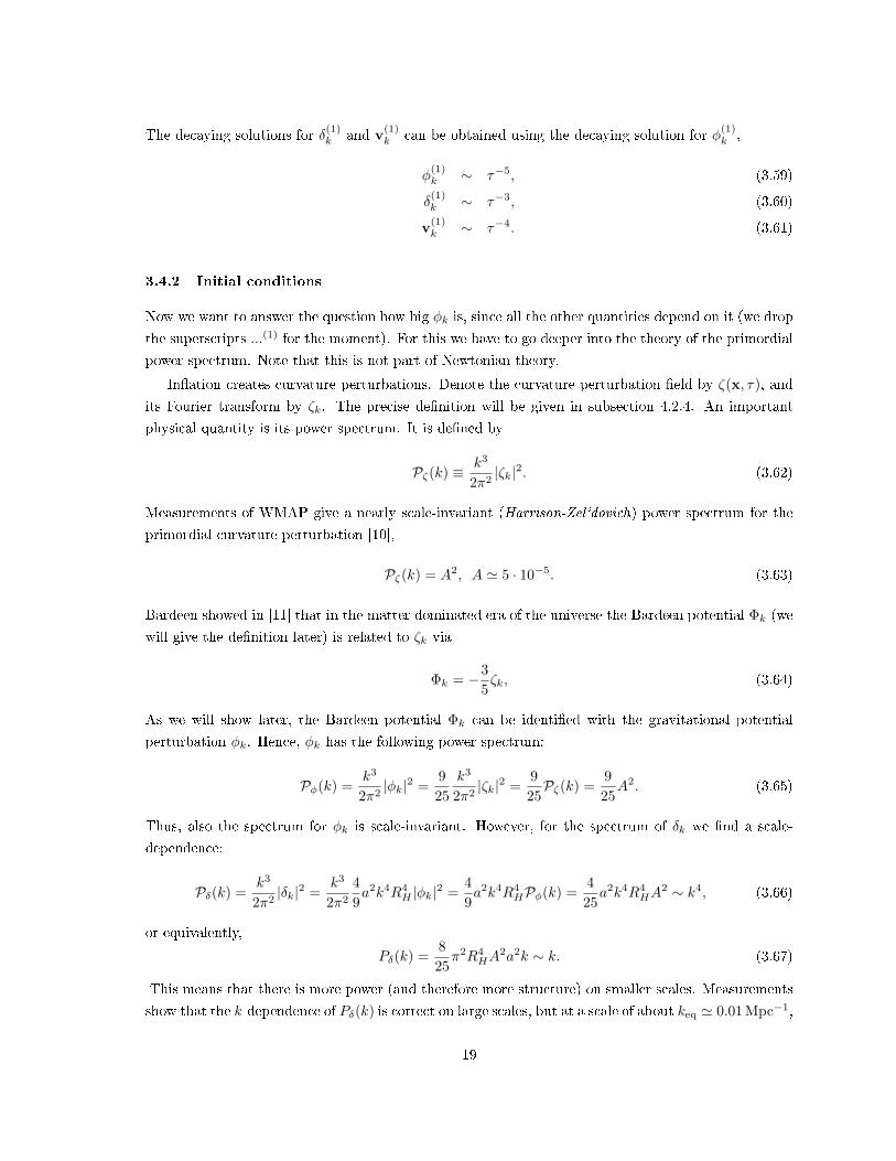
3.4.2 Initial conditions
Now we want to answer the question how big φk is, since all the other quantities depend on it (we drop
the superscripts ...(1) for the moment). For this we have to go deeper into the theory of the primordial
power spectrum. Note that this is not part of Newtonian theory.
Ination creates curvature perturbations. Denote the curvature perturbation eld by ζ(x, τ), and
its Fourier transform by ζk. The precise denition will be given in subsection 4.2.4. An important
physical quantity is its power spectrum. It is dened by
Pζ(k) ≡ k3
2π2|ζk|2. (3.62)
Measurements of WMAP give a nearly scale-invariant (Harrison-Zel'dovich) power spectrum for the
primordial curvature perturbation [10],
Pζ(k) = A2, A ' 5 · 10−5. (3.63)
Bardeen showed in [11] that in the matter dominated era of the universe the Bardeen potential Φk (we
will give the denition later) is related to ζk via
Φk = −3
5ζk, (3.64)
As we will show later, the Bardeen potential Φk can be identied with the gravitational potential
perturbation φk. Hence, φk has the following power spectrum:
Pφ(k) =k3
2π2|φk|2 =
9
25
k3
2π2|ζk|2 =
9
25Pζ(k) =
9
25A2. (3.65)
Thus, also the spectrum for φk is scale-invariant. However, for the spectrum of δk we nd a scale-
dependence:
Pδ(k) =k3
2π2|δk|2 =
k3
2π2
4
9a2k4R4
H |φk|2 =4
9a2k4R4
HPφ(k) =4
25a2k4R4
HA2 ∼ k4, (3.66)
or equivalently,
Pδ(k) =8
25π2R4
HA2a2k ∼ k. (3.67)
This means that there is more power (and therefore more structure) on smaller scales. Measurements
show that the k-dependence of Pδ(k) is correct on large scales, but at a scale of about keq ' 0.01 Mpc−1,
19

Figure 6: The matter power spectrum today, measured using various techniques [12]. The bendat k = keq ' 0.01 Mpc−1 is a result of the transition between radiation domination and matterdomination.
which is the scale that enters the horizon at the time of radiation-matter equality, the power spectrum
has a bend and decreases roughly as k−3 for higher k (see gure 6). This bend comes from the fact
that the universe was not always matter-dominated, but there was a radiation-dominated era (which
is not included so far in our model). In order to explain the bend, we have to nd out how density
perturbations grow during radiation domination.
3.4.3 Transfer function
As we discussed above, it is important that in the history of the universe there was a radiation-
dominated era, where the pressure was not zero. Therefore we consider now matter density pertur-
bations during radiation domination. However, we are going to neglect perturbations in the radiation
density, which turns out to be a good approximation. If we consider a universe that contains both
matter and radiation, we have to modify the Euler equation, containing both a gravitational potential
gradient and a pressure gradient. Then the rst order Newtonian equations are:
δ(1)′ +∇ · v(1) = 0, (3.68)
∆φ(1) = 4πGa2ρmδ(1), (3.69)
v(1)′ +Hv(1) = −∇(φ(1) +p(1)
ρ), (3.70)
20

where ρ = ρm + ργ is the total background energy density. Now we take the time derivative of eq.
(3.68) and subtract the divergence of eq. (3.70), using eq. (3.69) to replace ∆φ(1). This gives the
following relation:
δ(1)′′ +Hδ(1)′ = 4πGρma2δ(1) + ∆c2sδ
(1), (3.71)
where c2s = w = p(1)
ρ is the square of the speed of sound. In Fourier space this equation reads:
δ(1)′′k +Hδ(1)′
k = 4πGρma2δ
(1)k − k
2c2sδ(1)k . (3.72)
This equation is known as the growth equation or Jeans equation for δ(1)k [13]. The l.h.s. represents the
time change of δ(1)k , including a friction term Hδ(1)′
k , which is also called Hubble damping or Hubble
friction (the expansion of the universe slows down the growth of density perturbations). On the r.h.s.
there are two competitive sources: gravity, which supports the growth of density perturbations, and
pressure, which prevents it. It is convenient to introduce the comoving Jeans wavenumber,
kJ ≡(
4πGρma2
c2s
)1/2
, (3.73)
and the corresponding comoving Jeans length or Jeans scale,
λJ ≡ k−1J =
(4πGρma
2
c2s
)−1/2
. (3.74)
Then the Jeans equation can be written as
δ(1)′′k +Hδ(1)′
k = (k2J − k2)c2sδ
(1)k . (3.75)
Now we have two cases:
1. For scales much smaller than the Jeans length, k kJ , we can approximate the Jeans equation
by
δ(1)′′k +Hδ(1)′
k = −k2c2sδ(1)k . (3.76)
The solutions are oscillating with the frequency kcs, and the oscillations are damped by the
Hubble friction term, whence the amplitude of the oscillations decays with time. There is no
structure growth on sub-Jeans scales.
2. For scales much larger than the Jeans length, k kJ , we can approximate the Jeans equation
by
δ(1)′′k +Hδ(1)′
k = 4πGρma2δ
(1)k . (3.77)
During matter domination, this gives the growing solution δ(1)k ∼ a, which we already know.
During radiation domination, we have
ρm ρ ' ργ (3.78)
21

and hence
4πGa2ρm =3
2H2 ρm
ργ 1, (3.79)
so that we can neglect the source term on the right hand side. Then the Jeans equation becomes
δ(1)′′k +Hδ(1)′
k = 0, (3.80)
which has the general solution
δ(1)k = C1 + C2 ln a. (3.81)
Hence, during radiation domination density perturbations grow at most logarithmically on super-
Jeans scales.
Now we estimate the Jeans scale. During matter domination we have λJ = 0 since cs = 0, so that
perturbations grow on all scales. During radiation domination the speed of sound is cs =√
13 and
therefore kJ =√
3√
4πGρma2. As we approach the time of radiation-matter equality, we have ρm ≈ργ ≈ ρ
2 , whence kJ ≈ H. Thus, the Jeans scale grows to the size of the horizon at radiation-matter
equality and reduces to zero when matter dominates. Consequently, it makes a dierence if a scale
enters the horizon during radiation domination or during matter domination because perturbations
on scales that enter during radiation domination experience a suppression in growth. Now we want
to quantify this eect. First consider a density perturbation on a scale k−1 > k−1eq , which enters the
horizon during matter domination. At a later time af during matter domination it has grown by a
factor:δ
(1)k (af )
δ(1)k (aenter)
=H2
enter
H2f
=k2
H2f
. (3.82)
Now consider a perturbation on a scale k−1 < k−1eq . This scale enters the horizon during radiation
domination. But then, between the time it enters and the time matter takes over nothing happens to
the perturbation. Thus,
δ(1)k (af )
δ(1)k (aenter)
=δ
(1)k (af )
δ(1)k (aeq)
=H2
eq
H2f
=k2
eq
H2f
=k2
eq
k2
k2
H2f
. (3.83)
Hence, the growth on this scale is suppressed by a factor
T (k) ≡k2
eq
k2(3.84)
compared to a scale that enters during matter domination. In the last equation we introduced the
transfer function T (k), which gives the decit in growth that perturbations on scales smaller than k−1eq
experience. It should have the following properties:
T 2(k) = 1 for k keq, (3.85)
T 2(k) ∼k4
eq
k4for k keq. (3.86)
22
0
0.1
0.2
0.3
0.4
0.5
0.6
0.7
0.8
0.9
1
1e-04 0.001 0.01 0.1 1
T(k
)
k [Mpc-1]
simple transfer functionBBKS transfer function
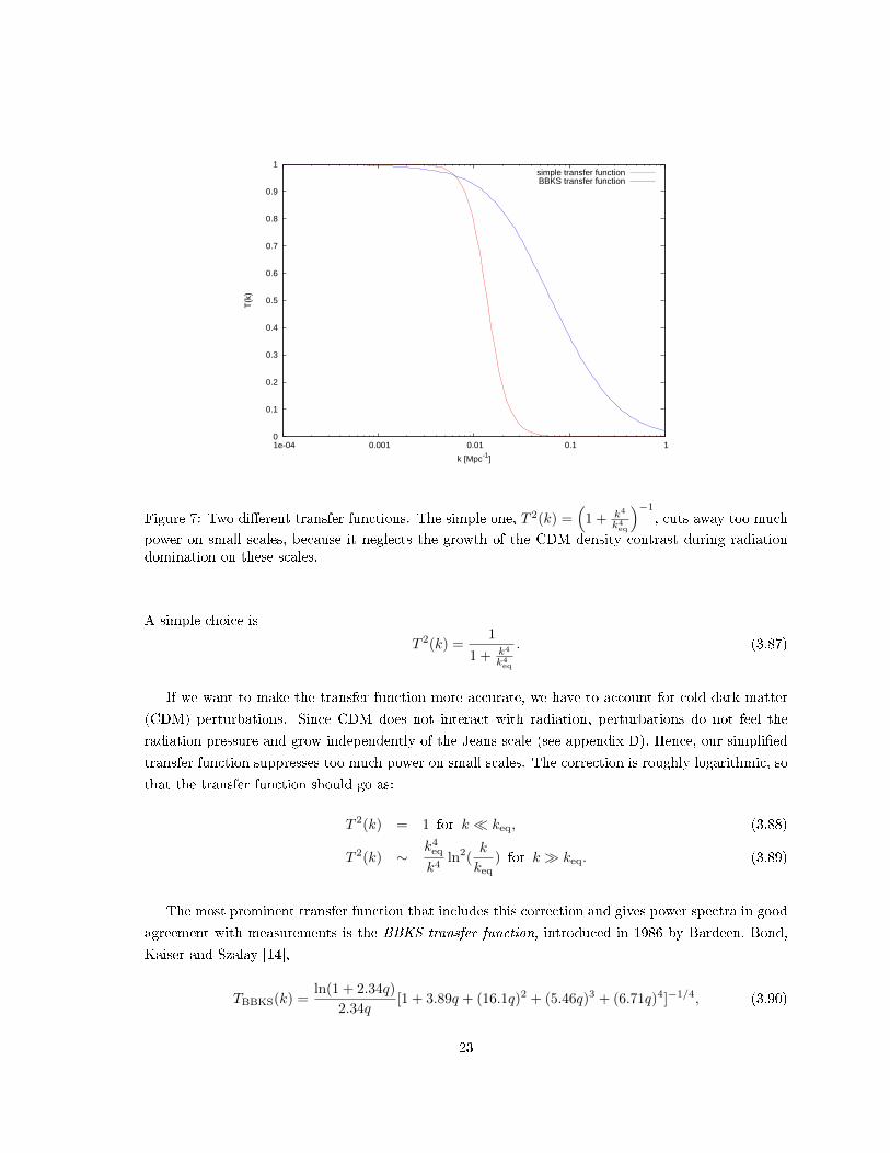
Figure 7: Two dierent transfer functions. The simple one, T 2(k) =(
1 + k4
k4eq
)−1
, cuts away too much
power on small scales, because it neglects the growth of the CDM density contrast during radiationdomination on these scales.
A simple choice is
T 2(k) =1
1 + k4
k4eq
. (3.87)
If we want to make the transfer function more accurate, we have to account for cold dark matter
(CDM) perturbations. Since CDM does not interact with radiation, perturbations do not feel the
radiation pressure and grow independently of the Jeans scale (see appendix D). Hence, our simplied
transfer function suppresses too much power on small scales. The correction is roughly logarithmic, so
that the transfer function should go as:
T 2(k) = 1 for k keq, (3.88)
T 2(k) ∼k4
eq
k4ln2(
k
keq) for k keq. (3.89)
The most prominent transfer function that includes this correction and gives power spectra in good
agreement with measurements is the BBKS transfer function, introduced in 1986 by Bardeen, Bond,
Kaiser and Szalay [14],
TBBKS(k) =ln(1 + 2.34q)
2.34q[1 + 3.89q + (16.1q)2 + (5.46q)3 + (6.71q)4]−1/4, (3.90)
23

where q ≡ kΓhMpc−1 and the shape parameter Γ is given by
Γ ≡ Ω0h exp(−Ωb −√
2hΩbΩ0
), (3.91)
where Ω0 is the relative energy density of the universe today and Ωb is the relative baryon density
today. Henceforth, we will use the BBKS transfer function with the parameters Ω0 = 1, Ωb = 0.05
and h = 0.7. We show a plot of the two dierent transfer functions in gure 7.
The transfer function connects the real power spectrum and the power spectrum from the Einstein-
de Sitter model. Hence, we make the following transformation:
P(k)→ T 2(k)P(k), (3.92)
The transfer function explains the bend in matter power spectrum (see gure 11). Furthermore, now
we can answer the question what the initial value for φ(1)k is. Including the transfer function, eq. (3.65)
becomes
Pφ(k) =k3
2π2|φ(1)k |
2 =9
25A2T 2(k). (3.93)
From this we nd the following initial value for φ(1)k :
|φ(1)k | =
3
5A(2π2)1/2k−3/2T (k). (3.94)
3.4.4 Second order solutions
The second order equations do not decouple a priori; we have to neglect the vector parts of the rst
order quantities, which can be done since v(1)⊥ decays. The decoupled second order equations are:
scalar part vector part
continuity equation δ(2)′ +∇ · v(2)‖ = −∇ · (δ(1)v
(1)‖ ) -
Poisson equation ∆φ(2) − 4πGa2ρ(0)δ(2) = 0 -
Euler equation v(2)′‖ +Hv
(2)‖ +∇φ(2) = −v
(1)‖ · ∇v
(1)‖ v
(2)′⊥ +Hv
(2)⊥ = 0
Table 6: Decoupled second order equations.
The vector part of the Euler equation gives v(2)⊥ ∼ a−1 (again, this is a special case of the general
result that the vorticity vanishes at all orders in Newtonian theory, as we showed earlier), so we can
neglect the vector contribution to v(2) and set v(2) = v(2)‖ . Now consider the scalar equations: The
sources for the second order perturbations are products of rst order perturbations, which we have
written on the r.h.s. of each equation. There are hence two solutions. The homogeneous solutions
are obtained by ignoring the source terms, which gives the same time dependence as in rst order
perturbation theory. However, the specic solutions grow faster due to the source terms, so that we
can neglect the homogeneous solutions. Note that the term v(1) · ∇v(1) can also be written as ∇v(1)2
2 .
Now we need to be careful when transforming to momentum space, because products in x-space become
convolutions in k-space.
24

• In momentum space the expression v(1)2
becomes:
F [v(1) · v(1)](k)
=1
(2π)3(v ? v)(k)
=1
(2π)3
∫d3k′v(k′) · v(k− k′)
=− 1
(2π)3
1
9τ3
∫d3k′k′φ(k′) · (k− k′)φ(|k− k′|)
=− 1
(2π)2
1
9τ3
∫ ∞0
dk′∫ π
0
dϑ′k′2 sinϑ′(kk′ cosϑ′ − k′2)φ(k′)φ(√k2 + k′2 − 2kk′ cosϑ′).
• The expression ∇ · (δ(1)v(1)) becomes:
F [∇ · δ(1)v(1)](k)
=ik · 1
(2π)3(δ(1) ? v(1))(k)
=ik · 1
(2π)3
∫d3k′δ(1)(k′)v(k− k′)
=ik · 1
(2π)3
i
18τ3
∫d3k′k′2φ(k′)φ(|k− k′|)(k− k′)
=− 1
(2π)3
1
18τ3
∫d3k′k′2φ(k′)φ(|k− k′|)k · (k− k′)
=− 1
(2π)2
1
18τ3
∫ ∞0
dk′∫ π
0
dϑ′k′4 sinϑ′(k2 − kk′ cosϑ′)φ(k′)φ(√k2 + k′2 − 2kk′ cosϑ′),
where we set k = k
0
0
1
and k′ = k′
sinϑ′ cosϕ′
sinϑ′ sinϕ′
cosϑ′
, so that k · k′ = kk′ cosϑ′.
The second order evolution equations in momentum space are:
δ(2)′k − ik · v(2)
k = −F [∇ · (δ(1)v(1))], (3.95)
k2φ(2)k +
6
τ2δ
(2)k = 0, (3.96)
v(2)′k +
2
τv
(2)k + ikφ
(2)k = −ik1
2F [v(1) · v(1)]. (3.97)
Note that δ(1)v(1) ∼ τ3 and v(1) · v(1) ∼ τ2 in leading order. There are other solutions as well, which
can be obtained by combining decaying and growing modes of δ(1) and v(1). However, these solutions
are all decaying and can be neglected. Hence, it is reasonable to make the following ansatz by adjusting
25

the time dependence of the second order perturbations to the time dependence of the source terms:
δ(2)k = Ckτ
4, (3.98)
v(2)k = Dki
k
kτ3, (3.99)
φ(2)k = Ekτ
2. (3.100)
With this ansatz, we nd the following system of linear equations for the coecients Ck, Dk, Ek:
4Ck −Dkk = −F [∇ · δ(1)v(1)](k)τ−3, (3.101)
Ekk2 + 6Ck = 0, (3.102)
5Dk + Ekk = −1
2kF [v(1) · v(1)](k)τ−2. (3.103)
The solutions are obtained by rst solving the convolution integrals and then solving the system
of linear equations for the coecients. This is done numerically for three xed scales that we are
interested in: the galaxy scale (k−1 = 1 Mpc), the cluster scale (k−1 = 10 Mpc), and the supercluster
scale (k−1 = 100 Mpc). Figures 8, 9 and 10 show the plots of the rst and second order perturbations
on these scales. Note that we plot the dimensionless quantities ∆(1)δ ≡
√Pδ = k3/2
√2π2|δ(1)k | etc.
1e-12
1e-10
1e-08
1e-06
1e-04
0.01
1
100
1e-04 0.001 0.01 0.1 1
∆(a,
k=
1 M
pc-1
)
a
Φ1v1δ1Φ2v2δ2
Figure 8: Evolution of rst and second order perturbations for the scale k−1 = 1 Mpc.
26

1e-12
1e-10
1e-08
1e-06
1e-04
0.01
1
100
1e-04 0.001 0.01 0.1 1
∆(a,
k=
0.1M
pc-1
)
a
Φ1v1δ1Φ2v2δ2
Figure 9: Evolution of rst and second order perturbations for the scale k−1 = 10 Mpc.
1e-16
1e-14
1e-12
1e-10
1e-08
1e-06
1e-04
0.01
1
1e-04 0.001 0.01 0.1 1
∆(a,
k=
0.01
Mpc
-1)
a
Φ1v1δ1Φ2v2δ2
Figure 10: Evolution of rst and second order perturbations for the scale k−1 = 100 Mpc.
27
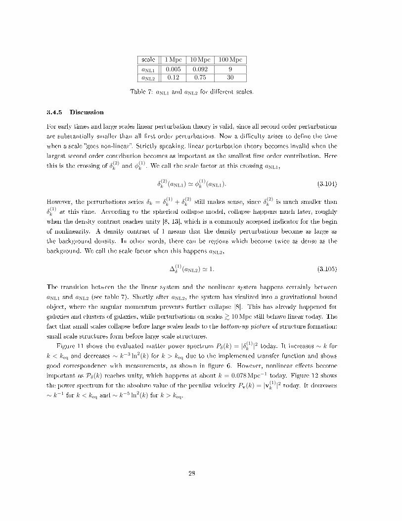
scale 1 Mpc 10 Mpc 100 Mpc
aNL1 0.005 0.092 9aNL2 0.12 0.75 30
Table 7: aNL1 and aNL2 for dierent scales.
3.4.5 Discussion
For early times and large scales linear perturbation theory is valid, since all second order perturbations
are substantially smaller than all rst order perturbations. Now a diculty arises to dene the time
when a scale goes non-linear. Strictly speaking, linear perturbation theory becomes invalid when the
largest second order contribution becomes as important as the smallest rst order contribution. Here
this is the crossing of δ(2)k and φ
(1)k . We call the scale factor at this crossing aNL1,
δ(2)k (aNL1) ' φ(1)
k (aNL1). (3.104)
However, the perturbations series δk = δ(1)k + δ
(2)k still makes sense, since δ
(2)k is much smaller than
δ(1)k at this time. According to the spherical collapse model, collapse happens much later, roughly
when the density contrast reaches unity [8, 13], which is a commonly accepted indicator for the begin
of nonlinearity. A density contrast of 1 means that the density perturbations become as large as
the background density. In other words, there can be regions which become twice as dense as the
background. We call the scale factor when this happens aNL2,
∆(1)δ (aNL2) ' 1. (3.105)
The transition between the the linear system and the nonlinear system happens certainly between
aNL1 and aNL2 (see table 7). Shortly after aNL2, the system has viralized into a gravitational bound
object, where the angular momentum prevents further collapse [8]. This has already happened for
galaxies and clusters of galaxies, while perturbations on scales & 10 Mpc still behave linear today. The
fact that small scales collapse before large scales leads to the bottom-up picture of structure formation:
small scale structures form before large scale structures.
Figure 11 shows the evaluated matter power spectrum Pδ(k) = |δ(1)k |2 today. It increases ∼ k for
k < keq and decreases ∼ k−3 ln2(k) for k > keq due to the implemented transfer function and shows
good correspondence with measurements, as shown in gure 6. However, nonlinear eects become
important as Pδ(k) reaches unity, which happens at about k = 0.078 Mpc−1 today. Figure 12 shows
the power spectrum for the absolute value of the peculiar velocity Pv(k) = |v(1)k |2 today. It decreases
∼ k−1 for k < keq and ∼ k−5 ln2(k) for k > keq.
28

1e-12
1e-10
1e-08
1e-06
1e-04
0.01
1
100
1e-04 0.001 0.01 0.1 1
∆ δ2 (a
=1,
k)
k [Mpc-1]
100
1000
10000
100000
1e-04 0.001 0.01 0.1 1
Pδ
[Mpc
3 ]
k [Mpc-1]
Figure 11: The matter power spectrum today. The top gure shows Pδ(k) and the bottom gureshows Pδ(k). Linear theory fails when Pδ(k) & 1 (vertical line).
29

1e-11
1e-10
1e-09
1e-08
1e-07
1e-06
1e-05
1e-04
1e-04 0.001 0.01 0.1 1
∆ v2 (a
=1,
k)
k [Mpc-1]
1e-05
1e-04
0.001
0.01
0.1
1
10
100
1000
10000
1e-04 0.001 0.01 0.1 1
Pv
[Mpc
3 ]
k [Mpc-1]
Figure 12: The power spectrum of |v| today. The top gure shows Pv(k) and the bottom gure showsPv(k).
30

3.4.6 Solutions during Λ-domination
As we approach a = 1, the cosmological constant becomes more and more important, as matter scales
∼ a−3. During Λ-domination the Friedmann and Raychaudhuri equations become
H2 =8πG
3a2ρΛ, (3.106)
H′ =8πG
3a2ρΛ. (3.107)
However, if we neglect dark energy perturbations, there are no variations in the rst order equations.
Hence, the form of the Jeans equation remains unchanged,
δ(1)′′k +Hδ(1)′
k = 4πGρma2δ
(1)k . (3.108)
Note that
4πGρma2 =
3
2H2 ρm
ρΛ 1, (3.109)
so that the source term of the Jeans equation becomes negligible. Then we have two solutions, the
growing solution
δ(1)k = const. (3.110)
and the decaying solution
δ(1)k ∼ a−2. (3.111)
Hence, as we approach Λ-domination, the density perturbations freeze out. A more general solution in
the intermediate regime, when dark energy and matter density are equally important, will be discussed
later, in section 5.3.
3.5 Newtonian cosmological simulations
Cosmological N -body simulations use Newton's equation of motion to simulate the behaviour of a xed
number of particles under the inuence of their reciprocal gravitational interaction. These simulations
are usually run in a box with periodic boundary conditions. In the (t, r)-system the equation of motion
can be written asd2ri(t)
dt2= −∇rφsim, (3.112)
where ri(t) is the trajectory of the i-th particle. Transforming to the (τ,x)-system, we nd
d
adτ
d
adτ(axi(τ)) =
1
a∇φsim. (3.113)
The l.h.s. is
d
adτ
d
adτ(axi(τ)) =
d
adτ
(Hxi(τ) +
dxi(τ)
dτ
)=
1
a
(H′xi(τ) +Hdxi(τ)
dτ+dx2
i (τ)
dτ2
),
31
and on the r.h.s. the potential can be split into a background part and a perturbed part,
1
a∇φsim =
1
a∇(φsim + δφsim).
Subtracting the background (this is the Raychaudhuri equation), we nd
d2xi(τ)
dτ2+Hdxi(τ)
dτ= −∇δφsim. (3.114)
From this equation it can be seen that all freely falling observers (for which δφsim = 0) will become
resting observers after suciently long time, since dxi(τ)dτ ∼ 1
a . The gravitational potential perturbation
is obtained using the Poisson equation,
∆δφsim = 4πGa2δρsim, (3.115)
which is solved in Fourier space, where the matter density perturbation is calculated by counting
particles in cells,
δρsim(x, τ) = a−3∑i
miδD(x− xi(τ)). (3.116)
4 The perturbed universe: relativistic treatment
4.1 The perturbed metric
In relativistic cosmological perturbation theory we consider small perturbations on the homogenous
and isotropic FRW metric tensor and on the energy-momentum tensor and calculate how these per-
turbations develop in time, using the energy-momentum conservation equation and the Einstein eld
equations. For a detailed reference, see [15]. Our conventions are the following: Greek indices will
range from 0 to 3 and Latin indices from 1 to 3. ∇µ as well as an index ;µ denote a covariant
derivative with respect to the perturbed metric. We are going to drop the superscripts ...(1) here, since
we only consider linear perturbations. Background quantities are denoted with a bar.
The FRW metric in a at universe, using comoving coordinates and conformal time, is
gµν ≡ a2
(−1 0
0 δij
). (4.1)
Now consider a small perturbation of the background metric: gµν = gµν + δgµν . We dene the metric
perturbation
δgµν ≡ a2
(−2φ wi
wi −2eδij + 2hij
). (4.2)
wi and hij can be further decomposed into scalar, vector and tensor parts,
wi = w;i + w⊥i (4.3)
32

type elds constraints degrees of freedom
scalar perturbations φ,ψ,w,h - 4vector perturbations w⊥i , hi ∇iw⊥i = ∇ihi = 0 4tensor perturbations hTij ∇ihTij = (hT )ii = 0, hTij = hTji 2
Table 8: Degrees of freedom in linear perturbation theory.
and
hij = Dijh+ h(i;j) + hTij , (4.4)
where Dij is the symmetric traceless double-gradient operator,
Dij ≡ ∇i∇j −1
3δij∆. (4.5)
Note that w⊥i and hi are pure vector parts with zero divergence (∇iw⊥i = ∇ihi = 0) and hTij is
transverse (∇ihTij = 0), traceless ((hT )ii = 0) and symmetric (hTij = hTji). Thus, in rst order the
metric perturbations decouple:
δgµν = δgSµν + δgVµν + δgTµν (4.6)
= a2
(−2φ w;i
w;i −2ψδij + 2h;ij
)+ a2
(0 w⊥iw⊥i 2h(i;j)
)+ a2
(0 0
0 2hTij
), (4.7)
where we have introduced a new variable5,
ψ ≡ e+1
3∆h. (4.8)
Now that we have decomposed the metric perturbation, it is instructive to count the degrees of freedom,
see table 8. The result is that we have altogether 10 degrees of freedom in the metric perturbation.
However, four of them correspond to the freedom of coordinate choice, so that we can put further
restrictions on the metric, as will be discussed later. The decomposition into scalar, vector and tensor
parts is important for the physical interpretation. The scalar perturbations are the most important,
because they couple to density perturbations and give rise to structure formation. The vector per-
turbations are not very interesting in linear order, because they couple to rotations only, which are
decaying in an expanding universe due to angular momentum conservation. Tensor perturbations give
rise to gravitational waves.
4.2 Gauge transformations
There is no unique mapping between points in the background spacetime and points in the perturbed
spacetime. Indeed, there are innitely many mappings, all close to each other. Consequently, for
5Some authors introduce this quantity as the curvature perturbation. However, we will later introduce the curvatureperturbation according to the denition of Bardeen [11].
33

. ..P P P
xα
xα
xα
~
^
Figure 13: Illustration of two dierent gauge choices.
a given coordinate system of the background, there exist innitely many coordinate systems of the
perturbed spacetime. A coordinate transformation between these coordinate systems is called a gauge
transformation. Consider a point P in the background spacetime, whose coordinates are xα. Nowconsider two dierent coordinate systems in the perturbed spacetime, and denote them by xα andxα. In the xα-coordinates, the background point P corresponds to a point P (x). In the xα-
coordinates, this point corresponds to another point P (x), see gure 13 for an illustration. We have
by construction
xα(P ) = xα(P ) = xα(P ), (4.9)
because all coordinates refer to the same point in the manifold. Now one can ask the question: what
are the xα-coordinates of the point P? These clearly dier from the xα-coordinates and we denote
this dierence by ξα, which is rst-order small due to the fact that all coordinate systems are close to
each other:
xα(P ) = xα(P ) + ξα, (4.10)
xα(P ) = xα(P ) + ξα. (4.11)
Note that it does not matter, in which coordinate system we give ξα, because the dierence is second
order. The above equations represent a coordinate transformation, which in cosmological perturbation
theory is called gauge transformation. They are equivalent to:
xα(P ) = xα(P )− ξα, (4.12)
xα(P ) = xα(P )− ξα. (4.13)
34

4.2.1 Gauge transformations of scalars, vectors and tensors
Using these transformations, we can determine how various geometric objects (scalars, vectors and
tensors) transform under a gauge transformation.
• First, let us determine the transformation of a scalar. Using Taylor expansion, we nd
s(P ) = s(P ) +∂s
∂xα(xα(P )− xα(P ))︸ ︷︷ ︸
−ξα
(1)= s(P )− ∂s
∂xαξα
(2)= s(P )− s′ξ0. (4.14)
Here we have used that (1) the dierence between ∂s∂xα and ∂s
∂xα is rst order small and can be
neglected when multiplied by ξα and (2) the background value s only depends on conformal time
τ , because the background spacetime is isotropic. The scalar perturbation in a given gauge is
dened as δs ≡ s(P )− s(P ) (or δs ≡ s(P )− s(P )). The transformation law is
δs = s(P )− s(P ) = s(P )− s(P )− s′ξ0 = δs− s′ξ0. (4.15)
Hence, any scalar that is constant in the background (s′ = 0) is gauge-invariant.
• For a vector wµ(P ) we have (µ refers to the coordinates xµ):
wµ(P ) = wµ(P )− ∂wµ∂xα
ξα (4.16)
and therefore
wµ(P ) =∂xσ
∂xµwσ(P ) =
∂(xσ − ξσ)
∂xµ(wσ(P )− ∂wσ
∂xαξα)
= (δσµ − ξσ,µ)(wσ(P )− ∂wσ∂xα
ξα)
= wµ(P )− wµ,αξα − wσξσ,µ. (4.17)
For a vector perturbation we nd the transformation
˜δwµ = wµ(P )− wµ(P )
= ˆδwµ − wµ,αξα − wσξσ,µ. (4.18)
Obviously, any vector that vanishes in the background is gauge-invariant.
• For a (0,2)-tensor Bµν(P ) we have:
Bµν(P ) = Bµν(P )−Bµν,αξα = Bµν(P )− Bµν,αξα (4.19)
35

and therefore
Bµν(P ) =∂xρ
∂xµ∂xσ
∂xνBρσ(P )
=∂(xρ − ξρ)
∂xµ∂(xσ − ξσ)
∂xν(Bρσ(P )− Bρσ,αξα)
= (δρµ − ξρ,µ)(δσν − ξσ,ν)(Bρσ(P )− Bρσ,αξα)
= Bµν(P )− Bµν,αξα − ξρ,µBρν − ξσ,νBµσ. (4.20)
For a tensor perturbation we nd
˜δBµν = Bµν(P )− Bµν(P )
= ˆδBµν − Bµν,αξα − ξρ,µBρν − ξσ,νBµσ. (4.21)
Again, any tensor that vanishes on the background is gauge-invariant.
4.2.2 Gauge transformation of metric perturbations
Now we can evaluate how the metric perturbation transforms. Using that the background metric is
symmetric and homogeneous, eq. (4.21) gives:
˜δgµν = ˆδgµν − g′µνξ0 − 2ξ(µ,ν). (4.22)
• The (0, 0)-component of eq. (4.22) reads, using the metric tensor from eq. (4.1) and the perturbed
part of the metric from eq. (4.2):
−2a2φ = −2a2φ+ 2aa′ξ0 + 2a2ξ0′
⇒ φ = φ−Hξ0 − ξ0′. (4.23)
• From the (0, i)-component of eq. (4.22) we nd the transformation of wi:
−a2wi = −a2wi − 2ξ(0,i)
= −a2wi − a2ξ0,i + a2ξ′i
⇒ wi = wi + ξ0,i − ξ′i. (4.24)
This can be further decomposed using ξi = ξ,i + ξ⊥i ,
w = w + ξ0 − ξ′, (4.25)
w⊥i = w⊥i − ξ⊥′i . (4.26)
36

• The (i, j)-component of eq. (4.22) is:
− 2a2eδij + 2a2hij = −2a2eδij + 2a2hij − 2aa′δijξ0 − 2ξ(i,j). (4.27)
Note that ξ(i,j) can be split into a traceless part and a diagonal part:
ξ(i,j) =1
3ξk,kδij + ξ(i,j) −
1
3ξk,kδij .︸ ︷︷ ︸
traceless
(4.28)
The trace of eq. (4.27) gives the transformation of e:
e = e+Hξ0 +1
3ξk,k. (4.29)
If we take the traceless part of eq. (4.27), we nd the transformation of hij :
hij = hij − ξ(i,j) +
1
3δijξ
k,k. (4.30)
This can be further decomposed,
h = h− ξ, (4.31)
hi = hi − ξ⊥i , (4.32)
hTij = hTij . (4.33)
• From eq. (4.31) and eq. (4.29) we nd the transformation law for ψ,
ψ = ψ +Hξ0. (4.34)
4.2.3 Gauge transformations of velocity and density perturbations
Next, consider the transformation of the peculiar velocity v. We have:
vi =dxi
dτ=d(xi + ξi)
d(τ + ξ0)=d(xi + ξi)
dτ
(d(τ + ξ0)
dτ
)−1
= (vi + ξi′)(1 + ξ0′)−1 = (vi + ξi′)(1− ξ0′) = vi + ξi′,
so that the velocity potential transforms as
v = v + ξ′, (4.35)
and the vector part transforms as
v⊥i = v⊥i + ξ⊥′i . (4.36)
37

For the density contrast δ we nd the transformation:
δ =δρ
ρ=δρ− ρ′ξ0
ρ= δ − ρ′
ρξ0 = δ + 3Hξ0. (4.37)
This means that v and δ depend on the gauge choice; they are dierent in each gauge. Hence, they
cannot be unique physical observables. However, it possible to construct gauge-invariant quantities,
which do not depend on the gauge choice, as we will show in the next subsection.
4.2.4 Gauge-invariant quantities
As mentioned before, unique physical quantities need to be gauge-invariant. A good example for this
is the theory of electromagnetism. Consider the free Lagrangian,
LEM = −1
4FµνFµν , (4.38)
where Fµν ≡ 2A(µ,ν) is the electromagnetic tensor and Aµ is the electromagnetic 4-potential. Note
that the Lagrangian is invariant under the gauge transformation
Aµ → Aµ + χ,µ. (4.39)
However, we can construct two gauge-invariant quantities out of Aµ, the electric eld
E ≡ A +∇A0 (4.40)
and the magnetic eld
B ≡ ∇×A. (4.41)
We can learn from this example that the question of gauge only arises in the theory. Once we evaluate
measurable quantities, the gauge should become irrelevant. However, here we ignored the role of the
observer. For example, if we consider a charge at a xed point, a resting observer would measure no
magnetic eld, while a moving observer would. This shows that also in electrodynamics the role of the
observer plays a crucial role.
Now let us come back to cosmological perturbation theory. We can construct gauge-invariant
combinations out of the perturbed quantities. The most famous ones are the Bardeen potentials [11],
Φ ≡ φ+1
a[(w − h′)a]
′, (4.42)
Ψ ≡ ψ −H(w − h′). (4.43)
Another important gauge-invariant quantity is the curvature perturbation, which we dene according
to Bardeen [11],
ζ ≡ 1
3δ + ψ. (4.44)
We introduced this quantity already in subsection 3.4.2, where we used its power spectrum to nd the
38

φ = 0 ψ = 0 δ = 0 w = 0 h = 0 v = 0
φ = 0 - / / S∗∗∗ ∗∗
∗∗∗
ψ = 0 / - / UC∗
SE∗
δ = 0 / / - UD∗
w = 0 S∗∗∗ UC
∗UD - N C
∗
h = 0 ∗∗ SE N - /
v = 0∗∗∗
∗ ∗C∗
/ -
Table 9: Gauges-overview. One can choose two dierent gauge conditions. A slash denotes combina-tions that are not possible. For some important gauges we introduce names. Stars denote residualgauge freedom (see text for explanation).
initial value for Φ. Other gauge-invariant quantities will be introduced later, in subsection 4.4.3.
4.2.5 Gauges
We can x the gauge by putting constrains on the metric perturbation elds or the uid perturbation
elds. Henceforth, we will only consider scalar perturbations and neglect all vector and tensor per-
turbations. This can be done since in rst order scalar, vector and tensor modes decouple. Then the
following transformations are relevant:
φ = φ−Hξ0 − ξ0′, (4.45)
ψ = ψ +Hξ0, (4.46)
w = w + ξ0 − ξ′, (4.47)
h = h− ξ, (4.48)
v = v + ξ′, (4.49)
δ = δ + 3Hξ0. (4.50)
Now we can choose two of these elds to be zero, which corresponds to choosing ξ0 and ξ. Note that
not all combinations are possible. One can only choose h or v to be zero (which xes ξ), as well as
one can only choose φ or ψ or δ to be zero (which xes ξ0). However, one can always choose w to
be zero, because this only xes the dierence between ξ0′ and ξ. In table 9 we show an overview over
the possible gauges one can construct by combining constrains on these perturbation elds. A slash
indicates a gauge that does not exist. For example, it is not possible to construct a gauge in which
both ψ and φ are zero, because then eq. (4.45) and eq. (4.46) would give contradicting expressions for
ξ0. The stars indicate the following residual gauge freedoms:
• * : There is a residual gauge freedom ξ → ξ + C(x), where C(x) is an arbitrary function.
39

• ** : There is a residual gauge freedom ξ0 → ξ0 + 1aD(x), where D(x) is an arbitrary function.
Hence, gauges with one and/or two stars are not unique, and we have to x the residual gauge freedom
(e.g. by setting C(x) = D(x) = 0). Furthermore, we have given some important gauges names in
order to refer to them:
• UC - uniform curvature gauge. In this gauge we set ψ = w = 0. One can show that in a spatially
at universe the 3-Ricci-scalar is given by (3)R = 4∆ψ (see [11]). Hence, in the uniform curvature
gauge, as well as in any other gauge with ψ = 0 there is no intrinsic curvature. These gauges
are hence a good choice for the comparison to Newtonian cosmology, where curvature does not
exist.
• SE - spatially Euclidean gauge. In this gauge we set ψ = h = 0, so that again the intrinsic
curvature vanishes. Furthermore, in this gauge the spatial part of the metric has no perturbation,
i.e. looks Euclidean. All perturbations are in the (0, 0)-part and the (0, i)-part of the metric.
• UD - uniform density gauge. In this gauge there are no density perturbations, since we set δ = 0.
• N - conformal Newtonian gauge. In this gauge we set w = h = 0. It is equivalent to the zero shear
gauge, σ = w = 0, where σ ≡ h′ + w generates the traceless part of the the extrinsic curvature
tensor and hence can be interpreted as the shear in the normal worldlines [11]. Another common
name for it is longitudinal gauge. Note that the metric perturbations φN and ψN coincide with
the Bardeen potentials in this gauge, φN = Φ and ψN = Ψ. Furthermore, it can be shown that Φ
corresponds to the gravitational potential introduced in Newtonian cosmology. For this, consider
a static universe6. The line element in conformal Newtonian gauge has the form
ds2 = gµνdxµdxν = −(1 + 2Φ)dτ2 + (1− 2Ψ)δijdx
idxj . (4.51)
The proper time between two events along a worldline is given by
∫ √−ds2 =
∫dτ
√1 + 2Φ− (1− 2Ψ)δij
dxi
dτ
dxj
dτ. (4.52)
Now we expand the integrand and keep only terms linear in Φ, Ψ and quadratic in v:∫ √−ds2 =
∫dt(1 + Φ− v2
2). (4.53)
The proper time is extremized if and only if the Lagrangian L = 1 + Φ− v2
2 satises the Euler-
Lagrange equation∂L
∂x=
d
dt
∂L
∂v, (4.54)
which yields Newton's law for the motion of particles,
v = −∇Φ. (4.55)
6A static universe has the nice simplications a = 1, dt = dτ , H = 0, u = v, x = r.
40

Figure 14: Illustration of slicing and threading, depending on the shift vector (here B) [8]. See textfor explanation.
Hence, the Bardeen potential Φ can be identied with the gravitational potential.
• C - comoving gauge. In this gauge we set w = v = 0. To explain what this means more vividly,
we need to introduce some new vocabulary. A gauge can be interpreted as a way of cutting the
4-dimensional spacetime into space and time. Hypersurfaces of constant τ give 3-dimensional
slices and worldlines of constant xi give 1-dimensional threads. The shift vector w tells how much
the coordinates of a point are shifted from one slice to the next slice. The shift vector vanishes if
and only if slicing and threading are orthogonal (see gure 14). The slicing is said to be comoving,
if the time slices are always orthogonal to the uid 4-velocity, which can be achieved by choosing
w = v. The threading is said to be comoving, if the threads are worldlines of comoving observers,
i.e. v = 0. The comoving gauge is dened by requiring both comoving slicing and comoving
threading [16, 8], which gives v = w = 0, or in the case of scalar perturbations, v = w = 0.
Hence, in the comoving gauge slicing and threading are orthogonal and the threads are worldlines
of comoving observers.
• S - synchronous gauge. In this gauge we set w = 0, so that comoving observers do not change
their coordinates from one time-slice to the next one, and φ = 0, so that observers at dierent
places have synchronous clocks (note that φ only aects the time-time component of the metric
tensor).
41

4.3 Relativistic equations in the conformal Newtonian gauge
In the conformal Newtonian gauge, the metric tensor is
gµν = a2
(−1− 2Φ 0
0 (1− 2Ψ)δij
)(4.56)
and the inverse metric is
gµν = a−2
(−1 + 2Φ 0
0 (1 + 2Ψ)δij
). (4.57)
Using the metric tensor, we can construct the connection coecients,
Γµαβ ≡1
2gµλ(gλβ,µ + gαλ,β − gαβ,λ). (4.58)
A calculation gives:
Γ000 = H+ Φ′, Γ0
0k = Φ,k, Γ0ij = (H− 2H(Φ + Ψ) + Ψ′)δij ,
Γi00 = Φ,i, Γi0j = (H−Ψ′)δij , Γikl = −(Ψ,lδik + Ψ,kδ
il ) + Ψ,iδkl.
The Ricci tensor is dened as
Rµν ≡ Γαµν,α − Γααµ,ν + ΓααβΓβµν − ΓαβµΓβαν . (4.59)
The components are:
R00 = −3H′ + 3ψ′′ + ∆Φ + 3H(Φ′ + Ψ′),
R0i = 2(Ψ′ +HΦ),i,
Rij = (H′ + 2H2)δij
+[−Ψ′′ + ∆Ψ−H(Φ′ + 5Ψ)− (2H′ + 4H2)(Φ + Ψ)]δij
+(Ψ− Φ),ij .
Raising an index we nd
R00 = 3a−2H′ + a−2[−3ψ′′ −∆Φ +−3H(Φ′ + Ψ′)− 6H′Φ],
R0i = −2a−2(Ψ′ +HΦ),i,
Ri0 = 2a−2(Ψ′ +HΦ),i,
Rij = a−2(H′ + 2H2)δij
+a−2[−Ψ′′ + ∆Ψ−H(Φ′ + 5Ψ)− (2H′ + 4H2)(Φ + Ψ)]δij
+a−2(Ψ− Φ),ij .
42

The Ricci scalar is
R ≡ R00 +Rii
= 6a−2(H′ +H2)
+a−2[−6Ψ′′ + 2∆(2Ψ− Φ)− 6H(Φ′ + 3Ψ′)− 12(H′ +H2)Φ].
Finally, we can construct the Einstein tensor Gµν ≡ Rµν − 12Rδ
µν ,
G00 = −3a−2H2 + a−2[2∆Ψ + 6HΨ′ + 6H2Φ],
G0i = R0
i = −2a−2(Ψ′ +HΦ),i,
Gi0 = Ri0 = 2a−2(Ψ′ +HΦ),i,
Gij = Rij −1
2Rδij
= a−2(−2H′ −H2)δij
+a−2[2Ψ′′ + ∆(Φ−Ψ) +H(2Φ′ + 4Ψ′) + (4H′ + 2H2)Φ]δij
+a−2(Ψ− Φ),ij .
The energy-momentum tensor for a perfect uid with zero pressure is
Tµν ≡ ρuµuν = ρ(1 + δ)uµuν . (4.60)
For the 4-velocity uµ we nd, using the normalization condition uµuµ = gµνu
µuν = −1,
uµ =1
a
(1− Φ
vN,i
), (4.61)
uµ = a
(−1− Φ
vN,i
). (4.62)
Note that vN = ∇vN , since we only consider scalar perturbations. Thus, the energy-momentum tensor
up to linear order is:
Tµν =
(−ρ(1 + δN ) ρvN,i
−ρvN,i 0
). (4.63)
Now we consider the Bianchi identity or relativistic energy-momentum conservation equation,
∇µTµν = 0. (4.64)
First consider the (ν = 0)-component of this equation. At background order, this gives the continuity
equation that we know already from Newtonian physics,
ρ′ + 3Hρ = 0, (4.65)
43

while the perturbed part gives the relativistic version of the perturbed continuity equation,
δ′N + ∆vN − 3Ψ′ = 0. (4.66)
Note the extra term −3Ψ′, which does not appear in Newtonian cosmology. Now consider the (ν = i)-
component of eq. (4.64). There is no background order of this equation because Tµi = 0. However, the
perturbed part of the (ν = i)-component gives the relativistic version of the perturbed Euler equation,
∇v′N +H∇vN = −∇Φ, (4.67)
which coincides exactly with the Newtonian equation.
Now consider the Einstein eld equations,
Gµν = 8πGTµν . (4.68)
To the background order, both sides are diagonal, and we have two equations: The (0, 0)-component
gives the Friedmann equation,
H2 =8πG
3ρa2, (4.69)
and the trace of the (i, j)-components gives the Raychaudhuri equation,
H′ = −4πG
3ρa2. (4.70)
At linear order however, there are 4 equations, the (0, 0)-component, the (0, i)-component, the trace
of the (i, j)-components, and the traceless part of the (i, j)-components. These are in conformal
Newtonian gauge:
3H2Φ + 3HΨ′ −∆Ψ = −4πGa2ρδN , (4.71)
Ψ′ +HΦ = −4πGa2ρvN , (4.72)
3Ψ′′ + 3H(Φ′ + 2Ψ′) + ∆(Ψ− Φ) + (2H′ +H2)Φ = 0, (4.73)
(Ψ− Φ),ij = 0. (4.74)
Note that the (0, 0)-component is the relativistic version of the Poisson equation, but the other equa-
tions do not have any counterpart in Newtonian physics. Hence, in relativistic cosmological perturba-
tion theory we have twice as much equations as in Newtonian cosmology.
4.4 Solutions
4.4.1 Solutions in the conformal Newtonian gauge
From eq. (4.74) we see that Φ and Ψ can only vary by some function of time, Φ−Ψ = f(τ). However,
since the mean value of a Gaussian perturbation vanishes (see appendix B), we must have f(τ) = 0.
44

Thus,
Φ = Ψ. (4.75)
Using this and the Raychaudhuri equation, eq. (4.73) becomes
Φ′′ + 3HΦ′ = 0. (4.76)
The decaying solution is Φ ∼ τ−5 ∼ a−3/2 and the growing one is
Φ = Φ(x). (4.77)
Both the growing and the decaying mode coincide with the solution for the gravitational pertur-
bation in the Newtonian case. From eq. (4.67) we nd the velocity potential,
vN = − 2Φ
3H. (4.78)
Again, this coincides with the velocity potential in the Newtonian case. Now consider the relativistic
Poisson equation, eq. (4.71), in Fourier space. Using the Friedmann equation 4πGa2ρ = 32H
2, Φ = Ψ
and Ψ′ = 0, we obtain:
δN = −2Φ− 2k2
3H2Φ. (4.79)
For scales that are small compared to the horizon, kH 1, this corresponds to the Newtonian result.
However, on scales larger than the horizon, kH 1, the density contrast stays constant.
4.4.2 Solutions in other gauges
We can construct solutions in other gauges using gauge transformations. For example, consider a
gauge transformation from the conformal Newtonian gauge (wN = hN = 0) to the uniform curvature
gauge (ψUC = wUC = 0). Equations (4.46) and (4.47) give
ξ0 = ξ′ =ψNH
=Φ
H. (4.80)
Then the density contrast in uniform curvature gauge is, according to eq. (4.50),
δUC = δN − 3Hξ0 = δN − 3Φ = −5Φ− 2k2
3H2Φ. (4.81)
Note that we express the density contrast in terms of the Bardeen potential Φ, so that the Newtonian
correspondence on small scales is satised. Hence, also in the uniform curvature gauge the density
contrast stays constant outside the horizon, however the value of this constant diers by a factor of 52 .
The density contrast in other gauges can be constructed in the same way. An overview can be
found in table 10, where we set all residual gauge modes to zero. Note that the density contrast in
the comoving gauge and in the synchronous gauge have the same form as in Newtonian cosmology.
However, in other gauges the density contrast stays constant outside the horizon. Plots of ∆δ = k3/2√
2π2|δ|
45

gauge N UC SE S C UD
φ Φ 52Φ 5
2Φ 0 0* − 59k2
H2 Φ
ψ Φ 0 0 53Φ 5
3Φ 53Φ + 2
9k2
H2 Φ
w 0 0 − ΦH 0 0 0
h 0 ΦH2 0 − 2
3H2 Φ − 23H2 Φ − 2
3H2 Φ− 13k2
H4 Φ
v - 23
1HΦ - 5
31HΦ - 2
31HΦ 0* 0 2
9k2
H3 Φ
δ −2Φ− 23k2
H2 Φ −5Φ− 23k2
H2 Φ −5Φ− 23k2
H2 Φ − 23k2
H2 Φ − 23k2
H2 Φ 0
3ζ −5Φ− 23k2
H2 Φ
Table 10: Overview - perturbations in conformal Newtonian (N), uniform curvature (UC), spatiallyEuclidean (UC), synchronous (S), comoving (C) and uniform density (UD) gauge. The quantity3ζ = δ − 3ψ is gauge-invariant. (* This is a result of the calculations and not the gauge condition.)
in dierent gauges can be found in gures 15 and 16. A discussion will follow in part 5.
4.4.3 Gauge-invariant solutions
In order to avoid the problem of gauge-dependence, one can consider only gauge-invariant perturba-
tions. However, then the diculty arises in interpreting these quantities, which is only possible if one
evaluates the gauge-invariant quantity in a specic gauge. As an example, consider the following three
dierent gauge-invariant combinations containing the density contrast, all introduced by Bardeen [17]:
• The quantity δGI,UC = δ − 3ψ = 3ζ reduces to δ in gauges where ψ = 0. Hence, it measures the
density contrast on hypersurfaces with zero curvature.
• The quantity δGI,N = δ−3H(w−h′) reduces to δ in a gauge where w = h = 0. Hence, it measures
the density contrast on longitudinal hypersurfaces, i.e. hypersurfaces whose normal unit vectors
have zero shear.
• The quantity δGI,C = δ−3H(v+w) reduces to δ in a gauge where v = w = 0. Hence, it measures
the density contrast on comoving hypersurfaces, i.e. from the point of view of the matter [17].
Expressed in terms of the Bardeen potential, these quantities are
δGI,UC = −5Φ− 2
3
k2
H2Φ, (4.82)
δGI,N = −2Φ− 2
3
k2
H2Φ, (4.83)
δGI,C = −2
3
k2
H2Φ. (4.84)
All three quantities coincide on scales well within the horizon, k H, but they dier signicantly
outside the horizon. Which of these gauge-invariant quantities can be considered as the physically
most appropriate is, as Bardeen formulated it, a matter of taste [17]. Thus, the introduction of
gauge-invariant variables does not solve the gauge problem. Instead of choosing a gauge, one has to
choose which gauge-invariant variable to take.
46

1e-06
1e-05
1e-04
0.001
0.01
0.1
1e-04 0.001 0.01 0.1 1
∆(a,
k=
0.01
Mpc
-1)
a
horiz
on e
ntry
δC,SδUC,SE
δNΦ
Figure 15: Evolution of the density contrast for k = 0.01 Mpc−1 in dierent gauges.
1e-08
1e-07
1e-06
1e-05
1e-04
0.001
1e-04 0.001 0.01 0.1 1
∆(a,
k=
0.00
1Mpc
-1)
a
horiz
on e
ntry
δC,SδUC,SE
δNΦ
Figure 16: Evolution of the density contrast for k = 0.001 Mpc−1 in dierent gauges.
47
4.5 Vector and tensor perturbations
So far we have ignored vector and tensor perturbations and considered only scalar perturbations. This
is possible, because in rst order they decouple from each other. For the same reason we can choose
the gauge condition for the scalar perturbations (this corresponds to choosing ξ0 and ξ) and the vector
perturbations (this corresponds to choosing ξ⊥) independently. Note that pure tensor perturbations
are per se gauge-invariant, so there is no gauge-choice for them.
As an example, we can choose a gauge with the scalar gauge condition w = h = 0 and the additional
vector gauge condition h = 0. We call this gauge the Poisson gauge (P), in agreement with [9]. The
gauge conditions can be reformulated in the form
∇iwiP = 0, (4.85)
∇ihijP = 0. (4.86)
Note that the scalar perturbations in the Poisson gauge are the same as the scalar perturbations
in the conformal Newtonian gauge. However, in the Poisson gauge, we have some additional vector
perturbation in the metric, wP = w⊥P 6= 0. Hence, in this gauge we nd the same equations for
scalar perturbations as in the conformal Newtonian gauge, but we nd some additional equations
for the vector perturbations, as shown in [9]. These are the vector parts of the Euler equation, the
(0, i)-component and the (i, j)-component of the Einstein equations (we drop the index P now - all
equations are given in Poisson gauge):
(v⊥i + w⊥i )′ +H(v⊥i + w⊥i ) = 0, (4.87)
1
2∆w⊥i = 8πGa2ρ(v⊥i + w⊥i ), (4.88)(
w⊥(i,j)
)′+ 2Hw⊥(i,j) = 0. (4.89)
From eq. (4.87) we nd a decaying solution for the vector perturbations,
v⊥i + w⊥i ∼ a−1. (4.90)
If there would have been some vector perturbations initially, they would have decayed, so our initial
approach to neglect all vector perturbations from the beginning is justied. However, note that this
argument only holds in rst order perturbation theory. At second order, there are couplings between
scalar and vector perturbations [18].
The only pure tensor perturbation that occurs is the transverse-traceless part of hij . In Poisson
gauge, we have hij = hTij , since h = 0 and h = 0. The only equation with a pure tensor part is the
transverse-traceless part of the (i, j)-component of the Einstein eld equations,
h′′ij + 2Hh′ij −∆hij = 0. (4.91)
48

Neglecting the Hubble friction, the solutions are gravitational waves,
hij ∼ ei(ωτ+k·x), (4.92)
with the dispersion relationω
k=∂ω
∂k= 1, (4.93)
which means that gravitational waves propagate with the speed of light. The Hubble drag term causes
the amplitude of these gravitational waves to decrease with time due to the expansion of the universe.
5 Quantication of relativistic corrections
In this part we quantify the relativistic corrections in cosmological N -body simulations and the ob-
served matter power spectrum. Furthermore, we discuss briey how the situation changes if one
considers a ΛCDM model instead of an Einstein-de Sitter model.
5.1 Relativistic corrections to Newtonian simulations
In the conformal Newtonian gauge and in the uniform curvature gauge the relativistic corrections for
the density perturbations on large scales and for early times become signicantly large. This can have
an impact on cosmological N -body simulations, which use Newtonian instead of relativistic equations.
These simulations typically start at z = 100 and the largest scales they simulate are about k−1 ' 1 Gpc.
We dene the relative error of the Newtonian density contrast compared to the relativistic one,
D(a, k) ≡ δGR − δNewton
δNewton, (5.1)
where we x the initial value for all solutions according to eq. (3.94). Plots of D(a, k) can be found in
gure 17. The relative error increases dramatically for large scales and early times: It is of the order
∼ 103% (∼4000% in the uniform curvature gauge and ∼2000% in the conformal Newtonian gauge) on
the 1 Gpc-scale at z = 100. For scales below 10 Mpc (galaxy and cluster scales) and redshifts below
z = 100, the error does not excess 1%. Hence, Newtonian simulations are more reliable on these scales.
Some authors [19, 20, 21] argue that Newtonian simulations are exact at linear order, if one uses
the following dictionary (one-to-one correspondence) between the simulated quantities and gauge-
invariant relativistic quantities:
δφsim ↔ Φ, (5.2)
vsim ↔ vGI,N, (5.3)
δsim ↔ δGI,C, (5.4)
where vGI,N = v + h′, so that it reduces the velocity potential on zero shear hypersurfaces. However,
there is a problem arising with this dictionary: While there is one set of equations connecting the
quantities on the left hand side (namely the Newtonian equations), there is not one set of equations
49
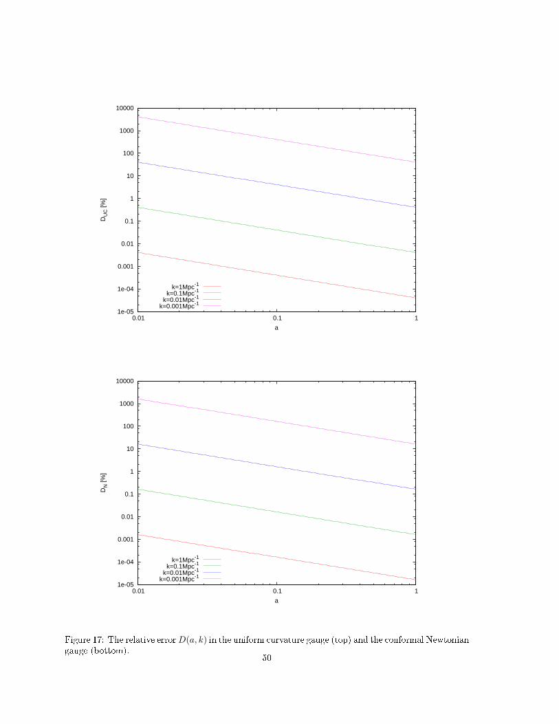
1e-05
1e-04
0.001
0.01
0.1
1
10
100
1000
10000
0.01 0.1 1
DU
C [%
]
a
k=1Mpc-1
k=0.1Mpc-1
k=0.01Mpc-1
k=0.001Mpc-1
1e-05
1e-04
0.001
0.01
0.1
1
10
100
1000
10000
0.01 0.1 1
DN
[%]
a
k=1Mpc-1
k=0.1Mpc-1
k=0.01Mpc-1
k=0.001Mpc-1
Figure 17: The relative errorD(a, k) in the uniform curvature gauge (top) and the conformal Newtoniangauge (bottom).
50

100
1000
10000
100000
1e+06
1e-04 0.001 0.01 0.1 1
Pδ
[Mpc
3 ]
k [Mpc-1]
horiz
on
C,SUC,SE
N
Figure 18: The matter power spectrum today in dierent gauges.
connecting the quantities on the right hand side. Indeed, this dictionary identies the simulated grav-
itational and velocity potentials with the relativistic counterparts on zero shear hypersurfaces, but the
simulated density contrast with the relativistic one on comoving hypersurfaces. This means that New-
tonian simulations are practically a mixture of relativistic simulations on two dierent hypersurfaces.
Furthermore, note that we cannot observe δGI,C since we are not observers on a comoving hypersurface.
A consistent dictionary would be the following,
δφsim ↔ Φ, (5.5)
vsim ↔ vGI,N, (5.6)
δsim ↔ δGI,N + 2Φ, (5.7)
where we identify all simulated quantities with gauge-invariant quantities that have a physical inter-
pretation on zero shear hypersurfaces.
5.2 Relativistic corrections to the observed power spectrum
Another interesting result is the rise of the matter power spectrum at very large scales, see gure 18.
At scales near the horizon today the relativistic power spectrum in the uniform curvature gauge is
about two orders of magnitude higher than in the the comoving/synchronous gauge. This rise of the
51

z kmin [Mpc−1]
1 1.25 · 10−3
0.6 1.75 · 10−3
0.3 2.98 · 10−3
Table 11: The minimal observable wavenumber for various redshifts.
power spectrum at large scales can be misinterpreted as primordial non-Gaussianity in the gravitational
potential perturbation, as pointed out by Yoo in [22] and by Zhang in [23]. As a next step we want to
nd out if this is an observable eect in the measured power spectrum at a given redshift. For this,
we introduce the distance-redshift relation in an Einstein-de Sitter universe [4],
d(z) =2
H0
(1− 1√
1 + z
). (5.8)
The minimal wavenumber one can observe at a given redshift is given by the inverse of d(z),
kmin =H0
2
π
1− 1√1+z
, (5.9)
where the extra factor π comes from the fact that we want to measure at least half a wavelength
(note that the relation between wavenumber and wavelength is k = 2πλ ). Table 11 shows kmin for the
redshifts z = 0.3, z = 0.6 and z = 1. In gure 19 we show the matter power spectra for these redshifts,
where the vertical bar denotes kmin. The dierence due to the gauge choice can become signicantly
large: At a redshift of z = 1, the power spectrum at the minimal observable wavenumber is about
twice as high in the uniform curvature gauge as it is in the comoving gauge.
For completeness we also show the velocity power spectrum Pv(k) = |vk|2 today in dierent gauges
in gure 20. In the conformal Newtonian and the spatially Euclidean gauge it corresponds to the
Newtonian power spectrum, see gure 12. However, in the uniform curvature gauge the spectrum is
higher by a factor of 254 . In the uniform density gauge the spectrum has a totally dierent shape.
Thus, the property that all gauges coincide on sub-horizon scales, which we found in the case of
density perturbations, is not true for velocity perturbations. Note that in the comoving gauge and in
the synchronous gauge the spectrum is zero because the peculiar velocity vanishes in these gauges, see
table 10.
5.3 Relativistic corrections in ΛCDM models
As we approach the present time, the cosmological constant gets more and more dominant. Today we
have ΩΛ ' 0.7, so that we should not neglect the eect of Λ. We can include dark energy into our
equations by setting ρ = ρm + ρΛ and p = pm + pΛ, where ρΛ = Λ8πG = const. and pΛ = −ρΛ = − Λ
8πG .
Then the modied energy-momentum tensor is
Tµν = (ρ+ p)uµuν + pδµν . (5.10)
52

1000
10000
0.001 0.01
Pδ(
z=1)
[Mpc
3 ]
k [Mpc-1]
C,SUC,SE
N
1000
10000
0.001 0.01
Pδ(
z=0.
6) [M
pc3 ]
k [Mpc-1]
C,SUC,SE
N
1000
10000
0.001 0.01
Pδ(
z=0.
3) [M
pc3 ]
k [Mpc-1]
C,SUC,SE
N
Figure 19: The matter power spectrum between k = 0.001 Mpc−1 and k = 0.01 Mpc−1 in dierentgauges for the redshifts z = 1, z = 0.6 and z = 0.3. The vertical line denotes kmin, the minimalobservable wavenumber at the corresponding redshift.
53

1e-16
1e-14
1e-12
1e-10
1e-08
1e-06
1e-04
0.01
1
100
10000
1e-04 0.001 0.01 0.1 1
Pv
[Mpc
3 ]
k [Mpc-1]
N,SEUCUD
Figure 20: The velocity power spectrum today in dierent gauges.
Note that ρ+ p = ρm + ρΛ + pm + pΛ = ρm and p = pm + pΛ = − Λ8πG , so that we have
Tµν = ρmuµuν − ρΛδ
µν . (5.11)
Hence, the only change is in the background,
Tµν =
(−ρm − ρΛ 0
0 −ρΛδij
), (5.12)
while the perturbations remain unchanged,
δTµν =
(−ρmδN ρmvN,i
−ρmvN,i 0
). (5.13)
Now we calculate the corrections that appear in the background equations. First, consider the Bianchi
identity ∇µTµν = 0. For ν = 0 we found the mass continuity equation,
ρ′m + 3Hρm = 0, (5.14)
which remains unchanged, since Λ is constant in time. The (ν = i)-component of the Bianchi identity
still has no background part, which comes from the fact that Λ is constant in space. Now consider the
Einstein eld equations, Gµν = 8πGTµν . In the background, the (0, 0)-component gives the Friedmann
54

equation, which becomes now
H2 =8πG
3a2(ρm + ρΛ). (5.15)
The Raychaudhuri equation (trace of the (i, j)-components) becomes
2H′ +H2 = 8πGa2ρΛ, (5.16)
or, using the Friedmann equation,
H′ = −4πG
3a2(ρm − 2ρΛ). (5.17)
In terms of proper time the background equations are
˙ρm + 3Hρm = 0, (5.18)
H2 =8πG
3(ρm + ρΛ), (5.19)
a
a= −4πG
3(ρm − 2ρΛ). (5.20)
One can nd solutions to these background equations in terms of hyperbolic functions [24],
a(t) =
[Ωm
1− Ωm
]1/3
sinh2/3
(t
tΛ
), (5.21)
H(t) =2
3tΛcoth
(t
tΛ
), (5.22)
ρm(t) = ρΛ sinh−2
(t
tΛ
), (5.23)
where tΛ = 2√24πGρΛ
. Now consider the perturbed equations in conformal Newtonian gauge:
δ′ − k2v − 3Φ′ = 0, (5.24)
v′ +Hv = −Φ, (5.25)
3H2Φ + 3HΦ′ + k2Φ = −4πGa2ρmδ, (5.26)
Φ′ +HΦ = −4πGa2ρmv, (5.27)
Φ′′ + 3HΦ′ = −8πGa2ρΛΦ. (5.28)
These are the perturbed parts of the 0-component and the i-component of the energy-momentum
conservation equation, the (0, 0)-component, (0, i)-component and (i, i)-component of the Einstein
eld equations, respectively, where we already used Φ = Ψ, which follows from the traceless part
of the (i, j)-components, which remains unchanged. Note that the only change occurs in the (i, i)-
component, eq. (5.28), because the term 2H′+H2 is not zero any more as we leave matter domination.
An analytic solution of these equations is very dicult due to the non-triviality of the background
solutions. However, one can do a numerical integration of the above equations to nd the evolution of
55

Figure 21: Relative error D(z, k) (here denoted as ∆) between the relativistic density contrast inconformal Newtonian gauge and the Newtonian one. From top to bottom, the curves are for k =0.001 Mpc−1, k = 0.01 Mpc−1, k = 0.1 Mpc−1 and k = 1 Mpc−1, respectively [25].
the density contrast. This was done for example by Dent and Dutta in [25], where they also solved the
corresponding Newtonian equations numerically and plotted the relative error between the Newtonian
solution and the relativistic solution. The result is shown in gure 21: The relative errors become even
larger (∼ 104% today on 1 Gpc-scales) in ΛCDM models than in the Einstein-de Sitter model (where
we found at most ∼ 103% on these scales). Note that the relative error remains constant in time due
to the fact that the density perturbations freeze out as dark energy takes over.
56

6 Summary and outlook
In this thesis we studied the validity of Newtonian equations, as used in cosmological N -body simula-
tions at large cosmological scales. These simulations are used to test our understanding of the universe,
in particular the formation of galaxies and clusters of galaxies. We linearized these equations in order
to compare them to linear relativistic cosmological perturbation theory. The linear equations need to
be corrected on small scales due to nonlinear eects and on large scales due to relativistic eects. The
important results are the following:
• For typical density uctuations (≤ 1σ) linear theory is valid until the density contrast reaches
unity. This happened at a scale factor of aNL2 = 0.12 (corresponding to a redshift of zNL2 ' 7) on
galaxy scales and aNL2 = 0.75 (zNL2 ' 0.3) on cluster scales. Perturbations on supercluster scales
still behave linear today (all second order quantities are smaller than all rst order quantities).
• The behaviour of density perturbations on scales larger than the Hubble horizon is strongly gauge-
dependent. It turns out that in the synchronous and the comoving gauge the density contrast
behaves like in Newtonian theory. However, in the conformal Newtonian gauge, the spatially
Euclidean gauge and the uniform curvature gauge the density contrast is constant outside the
Hubble horizon.
• The relativistic corrections to the simulated density perturbations in Newtonian N -body sim-
ulations can become signicantly large. Assuming that the accurate description of the density
contrast on superhorizon scales is given in the uniform curvature gauge or the conformal New-
tonian gauge, the error of the density contrast in Newtonian simulations reaches up to ∼ 103%
on the 1 Gpc-scale at a redshift of z = 100. This error increases to ∼ 104% if we consider a
ΛCDM model instead of an Einstein-de Sitter model. For scales below 10 Mpc and redshifts
below z = 100, the error does not excess 1%, whence Newtonian simulations on these scales are
more reliable.
• The observed matter power spectrum diers on large scales in dierent gauges. For example, at
a redshift of z = 1, the power spectrum at the minimal observable wavenumber is about twice
as large in the uniform curvature gauge as it is in the comoving gauge. It remains an open
question which power spectrum we expect to measure from a theoretical point of view. Maybe
the gauge-dependence of the power spectrum is a cue that this is not at all the quantity we
should consider.
• We should not ask which gauge is the correct one. Indeed, perturbations in all gauges are
correct solutions of Einstein's equations - this is the basic principle of general relativity. Instead,
we should ask the following questions: Is there a chosen gauge which gives predictions that are
closest to our measurements? If yes, which gauge and why? Another possibility is that there is no
such chosen gauge and indeed all quantities that we measure are truly gauge-invariant quantities,
which we do not yet understand theoretically. We have to answer these questions rst before we
really know how reliable Newtonian N -body simulations at large cosmological scales are.
57

Appendix A
Helmholtz decomposition theorem
Bounded domain
Let v(r) be a smooth vector function on a bounded domain D ⊂ R3, v : D → R3. Then there exists a
scalar potential v and a vector potential Ω such that:
v = v‖ + v⊥, (A.1)
= ∇v +∇×Ω, (A.2)
with v‖ =∇v and v⊥ = ∇×Ω, ∀ r∈D. It follows that ∇ · v⊥ = 0 and ∇× v‖ = 0.
The proof is done by construction. One can solve
∇ · v‖ = ∇ · v, (A.3)
∇× v⊥ = ∇× v, (A.4)
using the relation
∆1
|r− r′|= −4πδ(r− r′). (A.5)
The solutions are given by
v = − 1
4π
∫Dd3r′∇′ · v(r′)
|r− r′|+
1
4π
∫∂D
dS′ · v(r′)
|r− r′|, (A.6)
Ω =1
4π
∫Dd3r′∇′ × v(r′)
|r− r′|− 1
4π
∫∂D
dS′ × v(r′)
|r− r′|. (A.7)
Unbounded domain
If the domain D is unbounded, i.e. D = R3, we have to make the restriction
|v(r)||r|
→ 0 as |r| → ∞, (A.8)
so that the second terms in v and Ω vanish. Then the solutions are given by
v = − 1
4π
∫Dd3r′∇′ · v(r′)
|r− r′|, (A.9)
Ω =1
4π
∫Dd3r′∇′ × v(r′)
|r− r′|. (A.10)
Hypertorus
Now let the domain D be a Hypertorus, D = T3, as used in numerical simulations, where one considers
a box with periodic boundary conditions. Since we have v(ra) = v(rb) and dS(ra) = −dS(rb) for two
58

opposite sites a and b of the hypertorus, the boundary terms in v and Ω vanish as in the case of the
unbounded domain.
Uniqueness
The Helmholtz decomposition is not unique. If the vector contains a constant part, which is both
divergence- and curl-free, it can be included in the longitudinal part or in the transverse part. Note
that in cosmology a constant vector stands in contradiction to the isotropy of the universe. In order
to have a unique decomposition, one has to assume natural boundary conditions, i.e. v = 0 at the
boundary of the domain. In particular, in the case of an unbounded domain, the boundary condition
is
v(|r| → ∞)→ 0. (A.11)
For consistency, we show that the peculiar velocity we found satises this condition in all gauges con-
sidered. We found |vk| ∼ kΦ ∼ k−1/2T (k) in the conformal Newtonian gauge, the uniform curvature
gauge and the spatially Euclidean gauge and |vk| ∼ k3Φ ∼ k1/2T (k) in the uniform density gauge (see
table 10). Now we will consider the general case |vk| ∼ knT (k) and show that its Fourier transform
vanishes for |x| → ∞ for all n ∈ R. We have
|v(x)| ∼∫d3k|vk|eik·x
∼∫d3kknT (k)eik·x
≤∫d3kkneik·x
∼∫ kUV
kIR
dk
∫ π
0
dθ sin θkn+2eikx cos θ
∼∫ kUV
kIR
dkkn+2 sin(kx)
kx,
where we introduced the ultraviolet cuto wavenumber kUV and the infrared cuto wavenumber kIR
(this is a reasonable assumption for a Harrison-Zel'dovich spectrum, see appendix B). Now we make
the substitution p ≡ kx, so that
|v(x)| ∼ 1
xn+3
∫ xkUV
xkIR
dppn+2 sin(p)
p
≤ 1
xn+3
∫ xkUV
xkIR
dppn+1
=1
xn+3
1
n+ 2xn+2(kn+2
UV − kn+2IR )
∼ 1
x.
59

for n 6= −2. For n = −2 we have
|v(x)| ≤ 1
x
∫ xkUV
xkIR
dpp−1
=1
xln
(kUV
kIR
)∼ 1
x.
Thus, the boundary condition v(|x| → ∞)→ 0 is satised in all gauges we considered in this thesis.
Appendix B
Statistical properties of Gaussian perturbations
A Gaussian perturbation
g(x) =
∫d3kg(k)eik·x (B.1)
is dened as a perturbation whose Fourier components have a Gaussian probability distribution,
Prob[g(k)] =1
2πs2k
exp(−|g(k)|2
2s2k
), (B.2)
where s2k is the variance. From this we see directly that the mean value of each Fourier component is
zero,
〈g(k)〉 = 0. (B.3)
Furthermore, if we assume homogeneity and isotropy of the perturbations, it follows that dierent
Fourier components satisfy the following normalization condition:
〈g(k)g(k′)〉 = δ(k + k′)P (k), (B.4)
where
P (k) ≡ |g(k)|2 (B.5)
is the power spectrum7.
Now we go back to coordinate space and nd the following relation:
〈g(x)〉 = 〈∫d3kg(k)eik·x〉
=
∫d3k〈g(k)〉eik·x
= 0.
7This commonly used denition of the power spectrum is formally wrong. Indeed, one should divide by a unit volume,so that the power spectrum has the correct dimension, namely Mpc3. However, this is only a formal issue, so this unitvolume is usually dropped.
60
Hence, the mean value of a Gaussian perturbation in coordinate space vanishes. This comes from the
fact that positive and negative deviations from the background value are equally probable. In other
words, the mean value of a perturbed quantity is its background quantity. Next, consider
〈g(x)g(y)〉 = 〈∫
d3k
(2π)3eik·x
∫d3k′
(2π)3eik′·yg(k)g(k′)〉
=
∫d3k
(2π)3eik·(x−y)P (k)
=
∫ ∞0
k2dk
2π2
sin(kr)
krP (k)
=
∫ ∞0
dk
k
sin(kr)
kr
k3
2π2P (k)︸ ︷︷ ︸
≡P(k)
,
where r ≡ |x− y| is the distance and
P(k) ≡ k3
2π2P (k) =
k3
2π2|g(k)|2 (B.6)
is the dimensionless (band) power spectrum. For r = 0 we have
〈g(x)2〉 =
∫ ∞−∞
d ln kP(k). (B.7)
This means that the power spectrum P(k) of g gives the contribution of a logarithmic scale interval
to the variance of g(x). A power-law spectrum is a power spectrum of the form
P(k) = A2(k
kpivot)n−1, (B.8)
where kpivot is a chosen reference scale, the pivot scale, A is the amplitude at this scale, and n is the
spectral index. For n = 1, the spectrum is scale-invariant,
P(k) = A2. (B.9)
This spectrum is also called the Harrison-Zel'dovich spectrum [8, 13]. Note that 〈g(x)2〉 is logarith-mically divergent for a Harrison-Zel'dovich spectrum. Therefore one usually denes a cuto-scale at
small scales (ultraviolet-cuto) and at large scales (infrared-cuto) in order to make the integral nite.
61
Appendix C
Perturbations in the inaton eld
For completeness, we consider here perturbations in the inaton eld, that lead to the important
curvature perturbations after ination. We start with the Lagrangian for the inaton eld:
L = −1
2ϕ,µϕ,µ − V (ϕ). (C.1)
Applying the Euler-Lagrange equations, we nd the eld equation for the inaton,
ϕ+ 3Hϕ+∇2rϕ+ V,ϕ = 0. (C.2)
Now we split the inaton eld into a background part and a perturbed part,
ϕ(r, t) = ϕ(t) + δϕ(r, t). (C.3)
Then, in zeroth order, the eld equation becomes
¨ϕ+ 3H ˙ϕ+ V,ϕ = 0, (C.4)
which we already found in section 2.3. In linear order the eld equation reads
δϕ+ 3H ˙δϕ−∇2rδϕ+ δϕV,ϕϕ = 0. (C.5)
In slow-roll approximation, i.e. V,ϕϕ VM2Pl' H2, we can neglect the last term on the left hand side.
The resulting equation becomes in Fourier space:
¨δϕk + 3H ˙δϕk +k2
a2δϕk = 0, (C.6)
where k is the comoving wavenumber of the considered scale. Now we can distinguish two cases:
• For early times, when 3H k2
a2 , that means before horizon exit, the inaton perturbation is
oscillating with a decaying amplitude, |δϕk| ∼ 1a .
• For late times, when 3H k2
a2 , that means after horizon exit, the solution is δϕk = const., or in
other words, δϕk freezes out.
Note that, because H ≈ const. during ination, all scales have similar behaviour. This leads to a
nearly scale-invariant power spectrum of inaton-, and hence, curvature perturbations8. Indeed, one
can even show that the spectral index is related to the slow roll parameters, as dened in section 2.3,
n− 1 = −6ε+ 2η, (C.7)
8Bardeen showed in [11] that curvature perturbations are related to inaton perturbations by ζ = −H δϕϕ. Hence,
their spectra dier only by a factor H2
ϕ2 , which is constant in the slow-roll approximation.
62

whence n ' 1 in slow-roll approximation [8].
Appendix D
Meszaros equation
The Meszaros equation gives the growth of cold dark matter density perturbations in the intermediate
regime between radiation domination and matter domination. Assume that the universe is lled with
cold dark matter and radiation to a comparable amount. Then the Friedmann and Raychaudhuri
equations are:
H2 =8πG
3(ρm + ργ), (D.1)
a
a= −4πG
3(ρm + 2ργ), (D.2)
where ρm is the (dark) matter density and ργ is the radiation density. It is helpful to introduce a new
time variable
y ≡ a
aeq=ρmργ, (D.3)
so that
y 1 ⇔ radiation domination,
y 1 ⇔ matter domination.
For cold dark matter perturbations the Jeans equation gives
δ + 2Hδ − 4πGρmδ = 0. (D.4)
Note that there is no pressure source term because we consider only cold dark matter, which does not
interact with radiation. Now we want to write this equation in terms of the new time variable y. To
do this, we use
4πGρm =3
2H2 y
1 + y, (D.5)
and the transformation of the time derivatives,
d
dt=dy
dt
d
dy= Hy
d
dy. (D.6)
After some calculation one nds the Jeans equation in terms of the new time variable,
d2δ
dy2+
2 + 3y
2y(y + 1)
dδ
dy− 3
2y(y + 1)δ = 0. (D.7)
63

This equation was rst derived by Meszaros [26] and hence carries his name, the Meszaros equation9.
The general solution is given by
δ(y) = C1δ1(y) + C2δ2(y), (D.8)
where C1 and C2 are constants and
δ1(y) = 1 +3
2y, (D.9)
δ2(y) = 3√
1 + y −(
1 +3
2y
)ln
√1 + y + 1√1 + y − 1
. (D.10)
We can reconstruct the solutions during radiation domination and matter domination by considering
the limits y 1 and y 1, respectively:
• During radiation domination (y 1) the leading order in δ2 is δ2 ∼ ln y ∼ ln a, and the leading
order in δ1 is a constant. Hence, δ2 is the growing mode and δ1 is the decaying mode.
• During matter domination (y 1) the leading order in δ1 is δ1 ∼ y ∼ a, and the leading order
in δ2 is δ2 ∼ y−3/2 ∼ a−3/2. Thus, now δ1 is the growing mode and δ2 is the decaying mode.
Appendix E
Identity of synchronous and comoving gauge
We claim that, neglecting residual gauge modes, the synchronous gauge, where φS = wS = 0, and
the comoving gauge, where vC = wC = 0, are identical gauges during matter domination in that all
perturbation variables are the same in both gauges. To see that, rst consider a gauge transformation
from a generic gauge G to the conformal Newtonian gauge N , where wN = hN = 0, which is given by
ξ0 = hG − wG, (E.1)
ξ = hG. (E.2)
This transformation is unique. Now consider a gauge transformation from the conformal Newtonian
gauge to another gauge where two of the triple (φ, w, v) are zero. The transformation rules are:
φ = Φ−Hξ0 − ξ0′, (E.3)
w = ξ0 − ξ′, (E.4)
v = vN + ξ′. (E.5)
9It is also possible to construct the Meszaros equation for the intermediate time interval between matter dominationand dark energy domination. However, this equation is dicult to solve analytically. Böhmer et al. constructed aw-Meszaros equation for the time between matter domination and domination of a component with arbitrary w, andthey were only able to nd two additional analytic solutions in the parameter space w ∈ [−1, 1], one for w = − 1
3and
one for w = 16[27].
64

Note that the transformation law for φ implies ξ0 = −vN ⇔ φ = 0, which follows from the Euler
equation during matter domination. Now there are three possibilities:
• Setting φ = w = 0 (synchronous gauge) implies ξ0 = ξ′ = −vN + Ca , whence v = C
a . We can set
the constant to zero, so that v = 0.
• Setting v = w = 0 (comoving gauge) implies ξ0 = ξ′ = −vN , whence also φ = 0.
• Setting φ = v = 0 implies ξ0 = −vN + Ca and ξ′ = −vN , whence w = C
a . Again, we can set the
constant to zero, so that w = 0.
Since all three gauges, in which two of the triple (φ, w, v) are zero, are achieved by choosing ξ0 = ξ′ =
−vN , they are identical. In particular, the comoving and the synchronous gauge are identical during
matter domination. Note that this only holds if we set all residual gauge modes to zero.
65

References
[1] C.L. Bennett et al., Four year COBE DMR cosmic microwave background observations: Maps
and basic results, Astrophys.J. 464:L1, 1996.
[2] J.R. Gott et al., A map of the universe, Astrophys.J. 624:463, 2003.
[3] V. Springel et al., Simulations of the formation, evolution, and clustering of galaxies and quasars,
Nature 435:629, 2005.
[4] V.F. Mukhanov, Physical Foundations of Cosmology, Cambridge University Press 2005.
[5] A.H. Jae, Cosmology (lecture notes), Imperial College London 2011.
[6] K. Freese, Observational Evidence for Dark Matter, Talk given at conference: Dark Matter and
Dark Energy, Lyon 2008, arXiv:0812.4005.
[7] S. Perlmutter, Status of the cosmological parameters, Int.J.Mod.Phys. A15S1:715, 2000.
[8] A.H. Liddle and D.H. Lyth, Cosmological Ination and Large-Scale Structure, Cambridge Uni-
versity Press 2000.
[9] E. Bertschinger, Cosmological Dynamics, in: Les Houches Session LX: Cosmology and Large Scale
Structure, North-Holland 1993, arXiv:9503125.
[10] D.N. Spergel et al., First year Wilkinson Microwave Anisotropy Probe (WMAP) observations:
Determination of cosmological parameters, Astrophys.J.Suppl. 148:175, 2003.
[11] J. M. Bardeen, Cosmological perturbations: From quantum uctuations to large scale structure,
Lectures given at 2nd Guo Shou-jing Summer School on Particle Physics and Cosmology, Nanjing,
China, Jul 1988.
[12] M. Tegmark, A.J.S. Hamilton and Y.-Z. Xu, The power spectrum of galaxies in the 2dF 100k
redshift survey, Mon.Not.Roy.Astron.Soc. 335:887, 2002.
[13] P.J.E. Peebles, The Large-Scale Structure of the Universe, Princeton University Press 1980.
[14] J.M. Bardeen, J.R. Bond, N. Kaiser and A.S. Szalay, The statistics of peaks of gaussian random
elds, Astrophys.J. 304:15, 1986.
[15] V.F. Mukhanov, H.A. Feldman and R.H. Brandenberger, Theory of cosmological perturbations,
Phys.Rept. 215:203, 1992.
[16] H. Kurki-Suonio, Cosmological Perturbation Theory (lecture notes), University of Helsinki 2010.
[17] J.M. Bardeen, Gauge invariant cosmological perturbations, Phys.Rev. D22:1882, 1980.
[18] J.-C. Hwang and H. Noh, Second-order perturbations of cosmological uids, Phys.Rev.
D76:103527, 2007.
66

[19] N.E. Chisari and M. Zaldarriaga, Connection between Newtonian simulations and general rela-
tivity, Phys.Rev. D83:123505.
[20] S.R. Green and R.M. Wald Newtonian and relativistic cosmologies, arXiv:1111.2997, 2011.
[21] J.-C. Hwang H. and Noh, Newtonian versus relativistic nonlinear cosmology, Gen.Rel.Grav 38:703,
2006.
[22] J. Yoo, General relativistic description of the observed galaxy power spectrum: Do we understand
what we measure?, Phys.Rev. D82:083508, 2010.
[23] P. Zhang, The exact analytical solution of the linear structure growth rate in LCDM cosmology
and its cosmological applications, Phys.Rev. D82:063510, 2011.
[24] O. Gron, A new standard model of the universe, Eur.J.Phys. 23:135, 2002.
[25] J.B. Dent and S. Dutta, On the dangers of using the growth equation on large scales, Phys.Rev.
D79:063516.
[26] P. Meszaros, Primeval black holes and galaxy formation, Astron.Astrophys. 38:5, 1975.
[27] C.G. Boehmer and G. Caldera-Cabral, Evolution of sub-horizon cold dark matter perturbations,
arXiv:1008.2852.
67

Acknowledgments
Firstly I want to thank my supervisor Prof. Dr. Dominik Schwarz for his great guidance, motiva-
tion and ideas during my research. Furthermore, I want to thank Chris Byrnes for his help on the
comprehension of the Mukhanov-paper, Matthias Rubart for his help on general cosmological ques-
tions, and Viktor Dick for his help on some tricky calculations concerning the Christoel symbols and
more. I also want to thank the whole theoretical physics work group, especially the cosmology work
group, for creating an enjoyable working atmosphere. Last but not least, I want to thank my friends,
especially Thomas Weiÿ and Thomas Hederer, and my family for their support during the last year.
68

Erklärung
Hiermit erkläre ich, dass ich die vorliegende Arbeit selbstständig verfasst und keine anderen als die
angegebenen Hilfsmittel verwendet habe. Bielefeld, im Januar 2012.
(Samuel Flender)
69