Embed Size (px)
Citation preview
Master Thesis submitted within the
UNIGIS MSc program Geographical Information Science & Systems
Interfaculty Department of Geoinformatics – Z_GIS Paris Lodron University of Salzburg
on
Mapping social vulnerability to
natural hazards within the context of the
SOS Children’s Village in Quito, Ecuador
by
Dipl.-Ing. Roman Breitfuss-Schiffer 104854, UNIGIS MSc 2017
Supervisor:
Dr. Stefan Kienberger
Thesis submitted in partial fulfilment of the requirements of the degree of
Master of Science (Geographical Information Science & Systems) – MSc (GIS)
Salzburg, 18.08.2019
Mapping social vulnerability to natural hazards
Science Pledge
I
Science Pledge
By my signature below, I certify that my thesis is entirely the result of my own work. I have cited all
sources I have used in my thesis and I have always indicated their origin.
Place, Date Signature
Mapping social vulnerability to natural hazards
Acknowledgments
II
Acknowledgments
The successful writing of this thesis would not have been possible without the support and
contribution of many people
First, I want to thank my supervisor Stefan Kienberger for providing me with the opportunity to be
part of the cooperation between the Interfaculty Department of Geoinformatics (Z_GIS) and SOS
Children’s Village International and to contribute to the ongoing research in the field of risk and
vulnerability assessment. In this context, I want to express my gratitude to Richard Resl and Marcelo
Landivar from UNIGIS in Quito, who helped with data acquisition regarding the study area.
Furthermore, I want to especially thank Pablo Cabrera-Barona, who provided me with results of his
study regarding deprivation and healthcare accessibility and supported me with the basic workflow of
accessing and extracting Ecuadorean census data.
Mapping social vulnerability to natural hazards
Abstract
III
Abstract
Climate change is projected to increase risks from natural hazards such as heat stress, extreme
precipitation, inland flooding, or landslides for people in urban areas due to population growth and
poor planning and insufficient implementation of mitigation strategies (Pachauri et al., 2014). Billions
of people are affected and threatened by natural and manmade disasters worldwide, while children are
disproportionally affected (International Federation of Red Cross and Red Crescent Societies, 2018;
SOS Children’s Villages International, 2017a; Wallemacq and Below, 2018).
International organizations such as SOS Children’s Villages International seek to tackle these threats
and challenges and aim to minimize weather- and conflict-related risks for local communities (SOS
Children’s Villages International, 2017a). Risk and vulnerability assessment programs (RIVA) play an
important role in the evaluation and strengthening of disaster preparedness and response capacities of
local communities by developing target trainings, closing communication gaps and pro-positioning of
vital resources (SOS Children’s Villages International, 2017a).
Based on the aims of RIVA, this thesis focuses on the social vulnerability to natural hazards in an
urban area and aims to quantify the social vulnerability through a composite index based on a
theoretical risk and vulnerability framework. Furthermore, the spatial representation of the social
vulnerability scores should enable the localization of hot spots and serve as a tool for risk
management. The study area is the city of Quito.
Literature review was carried out to derive a set of preliminary socio-economic and demographic
indicators and variables. After statistical and multivariate analysis and the derivation of statistically
based weights through PCA/FA, the variables were aggregated to form a composite social
vulnerability index. Hot and cold spot analysis (Getis-Ord Gi* statistics) revealed neighborhoods of
high interest in terms of social vulnerability. The approach proposed in this thesis made sure to be
independent from third parties throughout the process of creation of the composite index, and
therefore ruled out the possibility of delays caused by external factors.
The results show high social vulnerability scores mainly in the outskirts of the city of Quito.
Especially in the outermost south-western and south-eastern neighborhoods high social vulnerability is
concentrated. High values were also found in the outermost north-western part and along the western
city limit.
The findings of this study serve as decision support for local authorities in terms of locating vulnerable
neighborhoods regarding natural hazards and prioritizing intervention measures. Focusing on the
revealed hot spot neighborhoods could lead to a better understanding of vulnerability itself in the local
communities, raise awareness towards natural hazards and potentially change the behavior of people in
case of an emergency. Furthermore, the results provide an important contribution towards developing
an integrated risk management approach with the final goal of developing targeted risk mitigation
strategies.

Mapping social vulnerability to natural hazards
Table of contents
IV
Table of contents
1. Introduction and background ...................................................................................................... 1
1.1 Defining vulnerability................................................................................................................. 1
1.1.1 Social vulnerability ..................................................................................................................... 1
1.2 Assessing vulnerability ............................................................................................................... 3
1.2.1 Conceptual frameworks and models ........................................................................................... 3
1.2.2 Vulnerability indices................................................................................................................. 10
1.3 Aims and objectives ................................................................................................................. 11
2. Materials and methods .............................................................................................................. 13
2.1 Study area ................................................................................................................................. 13
2.1.1 SOS Children’s Village in Quito .............................................................................................. 14
2.1.2 Natural hazards in Quito ........................................................................................................... 14
2.2 Underlying data ........................................................................................................................ 16
2.2.1 Census data 2010 ...................................................................................................................... 16
2.2.2 Hazard data ............................................................................................................................... 16
2.2.3 Other data ................................................................................................................................. 17
2.3 Conceptual framework ............................................................................................................. 17
2.4 Constructing a composite index ............................................................................................... 19
2.4.1 Selection of indicators .............................................................................................................. 19
2.4.2 Data transformation .................................................................................................................. 22
2.4.3 Missing data and outliers .......................................................................................................... 22
2.4.4 Normalization ........................................................................................................................... 25
2.4.5 Multivariate analysis................................................................................................................. 25
2.4.6 Final selection of indicators ...................................................................................................... 31
2.4.7 Weighting ................................................................................................................................. 32
2.4.8 Aggregation .............................................................................................................................. 35
2.4.9 Hot and cold spot analysis ........................................................................................................ 36
2.4.10 Visualization and mapping ....................................................................................................... 36
3. Results ...................................................................................................................................... 37
3.1 Vulnerability variables ............................................................................................................. 37
3.2 Social vulnerability to natural hazards in the city of Quito ...................................................... 40
4. Discussion and outlook ............................................................................................................. 48
5. Summary and conclusion.......................................................................................................... 50
6. References ................................................................................................................................ 51
Appendix A ........................................................................................................................................... 57
Appendix B ........................................................................................................................................... 63
Mapping social vulnerability to natural hazards
List of figures
V
List of figures
Figure 1: Key spheres of the concept of vulnerability (Source: Birkmann, 2005). ................................................ 3
Figure 2: Bohle’s conceptual framework for vulnerability analysis (Source: Bohle, 2001). ................................. 5
Figure 3: The conceptual framework to identify disaster risk (Source: Bollin et al., 2003). ................................. 5
Figure 4: Vulnerability Framework defined by Turner et al. (Source: Turner et al., 2003). .................................. 6
Figure 5: Pressure and Release (PAR) model: the progression of vulnerability (Source: Wisner et al., 2004). .... 6
Figure 6: Cardona and Barbat’s framework for holistic approach to disaster risk assessment and management
(Source: Birkmann (2006a) based on Cardona and Barbat (2000)). ....................................................................... 7
Figure 7: The BBC conceptual framework (Source: Birkmann (2006a) based on Bogardi and Birkmann (2004)
and Cardona (2001 and 1999)). .............................................................................................................................. 8
Figure 8: Cutter’s hazard-of-place model (Source: Cutter, 1996) .......................................................................... 8
Figure 9: The MOVE framework (Source: Birkmann et al. (2013) based on concepts of Birkmann, 2006a;
Bogardi and Birkmann, 2004; Cardona, 2001, 1999; Carreño et al., 2007a; IDEA, 2005; Turner et al., 2003). .... 9
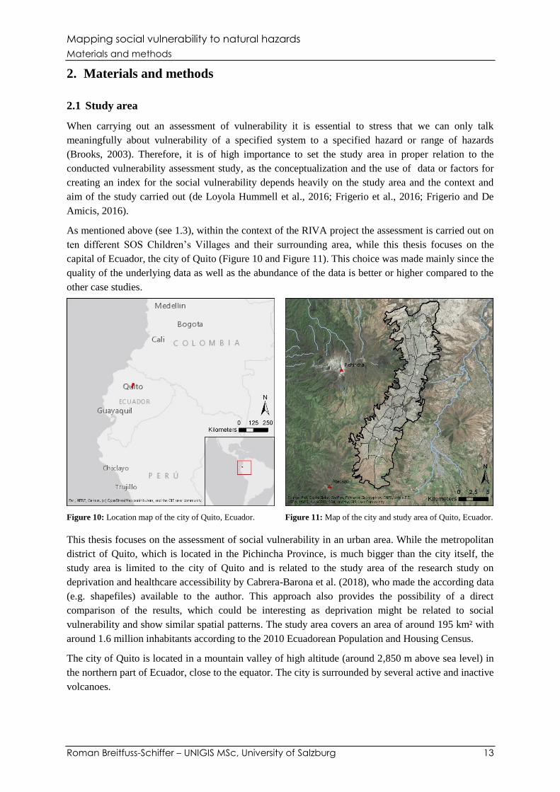
Figure 10: Location map of the city of Quito, Ecuador. ...................................................................................... 13
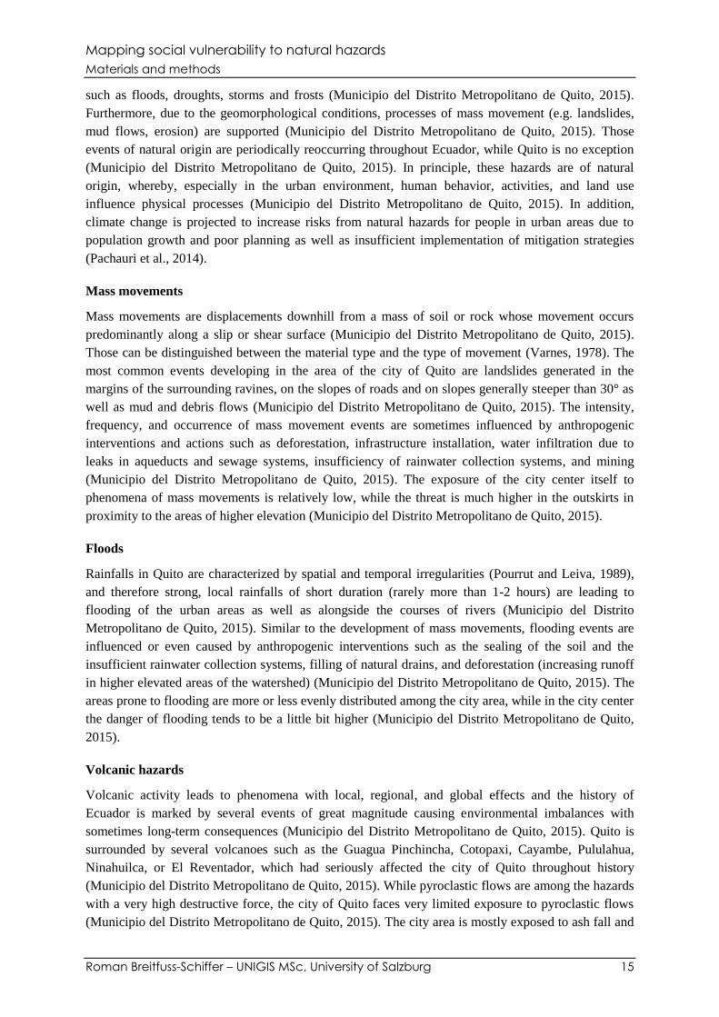
Figure 11: Map of the city and study area of Quito, Ecuador. ............................................................................. 13
Figure 12: Location of the SOS Children’s Village itself and other SOS CV premises in Quito. The district
Quitumbe is highlighted as it is considered for future extension by SOS CV. ..................................................... 14
Figure 13: Adapted MOVE risk and vulnerability framework based on Birkmann et al. (2013) – The assessment
is carried out on a subnational to local scale. The relevant domains are highlighted, while the exposure domain is
excluded from the assessment. .............................................................................................................................. 18
Figure 14: Workflow for the composite index construction process (adapted from Hagenlocher et al., 2013). .. 19
Figure 15: Box-and-whisker plots of the statistically problematic variables (excl. var. 10.3 & 14.1) with the
0.975 quantile marked in red. ................................................................................................................................ 24
Figure 16: Visualization of correlation matrices with values of Pearson’s r for each of the two vulnerability
domains (SUS – left, LoR – right). ....................................................................................................................... 26
Figure 17: Scree plots of eigenvalues from PCA for each of the two domains (SUS – left, LoR – right). .......... 28
Figure 18: Spatial distribution of the final selection of susceptibility (SUS) variables (min-max normalized
values) within the study area with the assigned weight. ....................................................................................... 37
Figure 19: Spatial distribution of the final selection of lack of resilience (LoR) variables (min-max normalized
values) within the study area with the assigned weight. ....................................................................................... 38
Figure 20: Social vulnerability to natural hazards in the city of Quito. ............................................................... 40
Figure 21: Distribution of social vulnerability to natural hazards in the city of Quito with the according mean
value and standard deviation. ................................................................................................................................ 41
Figure 22: Hot and cold spots of social vulnerability (Getis-Ord Gi*, fixed distance band, threshold distance
590.4 m). ............................................................................................................................................................... 41
Figure 23: Social vulnerability to natural hazards in the southern part of the city of Quito with locations of SOS
CV premises and highlighting of the district Quitumbe. ....................................................................................... 42
Figure 24: Relative contribution of the indicators to the social vulnerability composite index for three census
blocks in the northern part of the city of Quito. Orange colors in the pie chart represent the SUS domain, purple
colors represent the LoR domain. ......................................................................................................................... 43
Mapping social vulnerability to natural hazards
List of figures
VI
Figure 25: Relative contribution of the indicators to the social vulnerability composite index for three census
blocks in the district Quitumbe. Orange colors in the pie chart represent the SUS domain, purple colors represent
the LoR domain. .................................................................................................................................................... 44
Figure 26: Natural hazards (mass movements, floods, volcanic hazards, and forest fires) in the city of Quito with
hot spot areas of social vulnerability (polygon data of mass movements and volcanic hazards from RIVA project,
rest of the data from Quito Open Data). ................................................................................................................ 46
Mapping social vulnerability to natural hazards
List of tables
VII
List of tables
Table 1: Preliminary set/wish list of indicators with the according variables and domain (SUS – Susceptibility,
LoR – Lack of Resilience). Sign indicates if a higher value increases (+) or decreases (-) vulnerability. ............ 21
Table 2: Statistically problematic variables regarding potential outliers (skewness > 2.0, kurtosis > 3.5). ......... 23
Table 3: List of variables included in the treatment of outliers; the column 97.5 perc. lists the value of the 97.5
percentile. The column > 97.5 perc. lists the percentage of values exceeding the 97.5 percentile. ...................... 24
Table 4: VIF values for each variable of the two vulnerability domains. ............................................................ 26
Table 5: Variables with critical values of high collinearity based on thresholds for Pearson’s r and/or VIF....... 27
Table 6: Results of the PCA for each of the two domains with eigenvalues and the according explained variance
for each principal component. ............................................................................................................................... 28
Table 7: Component loadings of the retained first five principal components, loadings > ±0.30 are
highlighted. ........................................................................................................................................................... 29
Table 8: Rotated factor loadings for individual variables (SUS) of the retained factors using varimax rotation,
loadings > ±0.30 are highlighted. .......................................................................................................................... 30
Table 9: Rotated factor loadings for individual variables (LoR) of the retained factors using varimax rotation,
loadings > ±0.30 are highlighted. .......................................................................................................................... 31
Table 10: Final set of indicators with the according variables and domain (SUS – Susceptibility, LoR – Lack of
Resilience). Sign indicates if a higher value increases (+) or decreases (-) vulnerability. .................................... 32
Table 11: Rotated factor loadings for individual variables for each of the two domains, squared normalized
factor loadings, the highest loading (absolute value) for each variable is highlighted. ......................................... 33
Table 12: Indicators with the according variables, signs, and weights grouped by domain (SUS, LoR). ............ 34
Mapping social vulnerability to natural hazards
Introduction and background
Roman Breitfuss-Schiffer – UNIGIS MSc, University of Salzburg 1
1. Introduction and background
1.1 Defining vulnerability
Generally speaking, the meaning of the term vulnerability differs regarding the context in which it is
used (Miller et al., 2010). It has been applied as a core concept in various studies in different research
fields (e.g. disaster risk studies or economics), which has also led to conceptual differences (Miller et
al., 2010). Birkmann (2006a) states that there are more than 25 different definitions, concepts and
methods to describe vulnerability. When focusing on the context of disaster risk, the ambivalence still
remains as the term is widely spread and used with different meanings throughout distinct groups of
interest, such as the academia, disaster management agencies, the climate change community, and
development agencies (Villagran, 2006). Within the last decades, vulnerability assessment in the field
of natural hazards and climate change has gained of importance (Birkmann et al., 2013).
Already in 1989, Chambers (1989) introduced an important concept in which vulnerability basically
refers to “exposure to contingencies and stress, and difficulty in coping with them” (Chambers, 1989,
p.1). He proposed an external and internal side of vulnerability, whereas the external side is related to
risks, shocks and stress while the internal side is related to defenselessness and incapacity to cope with
damaging loss (Chambers, 1989). Furthermore, Chambers (1989) argues that vulnerability should not
be considered as equal to poverty but related.
In 2001, the IPCC Third Assessment Report describes vulnerability as “the degree to which a system
is susceptible to, or unable to cope with, adverse effects of climate change, including climate
variability and extremes. Vulnerability is a function of the character, magnitude, and rate of climate
change and variation to which a system is exposed, its sensitivity and its adaptive capacity” (IPCC,
2001, p.6). This definition embodies the starting point interpretation where vulnerability is viewed as
a general characteristic of societies generated by different social and economic factors and processes
while the contrasting end point definition views vulnerability as the residual of climate change impacts
minus adaption (the remaining segments of the possible impacts of climate change that are not
targeted through adaptation) (Bogardi et al., 2005; Villagran, 2006). This shows once more the
divergent meanings of the term vulnerability as well as the variations in the underlying concepts, even
within the climate change community (Kelly and Adger, 2000).
The International Strategy for Disaster Reduction (2004) defines vulnerability as “the conditions
determined by physical, social, economic, and environmental factors or processes, which increase the
susceptibility of a community to the impact of hazards” (ISDR, 2004, p.16). In this approach
vulnerability is classified in different components or factors (e.g. physical or social), which are again
related to different factors itself (ISDR, 2004).
It is evident that the above-mentioned definitions and descriptions of vulnerability represent only a
small extract of the different definitions in use. Nevertheless, it shows that the meaning of the term
differs, even within the community of one single scientific field.
1.1.1 Social vulnerability
The predominant views on vulnerability in most of the studies up to a certain point, especially when
focusing on climate change impact, concentrate on the physical dimensions of the issue (Adger, 1999).
Birkmann (2006a) stresses the need for a paradigm shift from hazard analysis to identification and
assessment of vulnerabilities, as the ability to measure vulnerability is increasingly being seen as a key
step towards effective risk reduction and the promotion of a culture of disaster resilience.
Mapping social vulnerability to natural hazards
Introduction and background
Roman Breitfuss-Schiffer – UNIGIS MSc, University of Salzburg 2
As already mentioned in the title, this thesis focuses on social vulnerability, which is one of the key
factors when describing vulnerability (Birkmann et al., 2013; ISDR, 2004). The problem of the
vagueness of the term vulnerability also applies to the usage of the concept of social vulnerability,
which means that different authors apply it differently (Birkmann, 2006a). Also Fatemi et al. (2017)
point out, that there is still a lack of a comprehensive definition meeting the requirements of various
social and humanistic disciplines.
Cannon et al. (2003) state that it is import to recognize “social vulnerability as much more than the
likelihood of buildings to collapse or infrastructure to be damaged” (Cannon et al., 2003, p.5). They
view social vulnerability as a person’s set of the following characteristics (Cannon et al., 2003, p.5):
- Initial well-being (nutritional status, physical and mental health)
- Livelihood and resilience (assets and capitals, income, qualifications)
- Self-protection (capability and willingness to build a safe home, use a safe site)
- Social protection (hazard preparedness provided by society more generally)
- Social and political networks and institutions (social capital, institutional environment)
In the definition of Cannon et al. (2003) it is evident that the processes and factors describing the
vulnerability condition are quite distant from the impact of a hazard itself. In addition, Cannon et al.
(2003) argue that social vulnerability is not equal to poverty, since poverty is a measure of current
status, whereas vulnerability should involve a predictive quality. Nevertheless, all the vulnerability
variables in their definition are inherently connected with peoples’ livelihoods and with poverty
(Cannon et al., 2003).
Based on two decades of research on this issue, Downing et al. (2006) view social vulnerability
characterized by six attributes. They argue that social vulnerability is (Downing et al., 2006, p.3)
- the differential exposure to stress experienced or anticipated by different exposure units,
- a dynamic process,
- rooted in the actions and multiple attributes of human actors,
- driven by social networks in social, economic, political and environmental interactions,
- constructed simultaneously on more than one scale,
- determined by multiple stresses.
In the definition of the ISDR (2004), the social factor of the vulnerability is characterized by multiple
factors itself. Thus, social vulnerability is, i.a., linked to the level of well-being of individuals or
communities, education, peace and security, access to human rights, social equity, gender, age, class or
caste privileges, public health, handicaps of individuals, and basic infrastructure (e.g. water supply and
sanitation) (ISDR, 2004, p.42).
In 2013, Birkmann et al. (2013) develop a holistic framework to systematize and assess vulnerability.
Therein, Social vulnerability is defined as the “propensity for human well-being to be damaged by
disruption to individual (mental and physical health) and collective (health, education services, etc.)
social systems and their characteristics (e.g. gender, marginalization of social groups)” (Birkmann et
al., 2013, p.200).
Apparently, social vulnerability relates to socio-economic factors and individual characteristics of
people (e.g. age, gender, health etc.), but also to place inequalities, i.e. characteristics of communities
and the built environment (e.g. level of urbanization, growth rates etc.) (Cutter et al., 2003).
Consequently, the concept of social vulnerability is more broadly used than just for the estimation of
traditional social aspects of vulnerability (e.g. gender, age, income etc.), but can include economic and
physical aspects, provided they are the expressions of a socially constructed vulnerability (Birkmann,

Mapping social vulnerability to natural hazards
Introduction and background
Roman Breitfuss-Schiffer – UNIGIS MSc, University of Salzburg 3
2006a). Hence, social vulnerability should not be limited to the estimation of the direct impacts of a
hazardous event, but it should be perceived as the estimation of the wider environment and social
circumstances encompassing the coping capacity and resilience of the concerned people and
communities (Birkmann, 2006a). The widening of the concept of vulnerability is illustrated in Figure 1
and it shows that starting from a general basic understanding, a process of broadening took place
(Birkmann, 2005, 2006a).
Figure 1: Key spheres of the concept of vulnerability (Source: Birkmann, 2005).
1.2 Assessing vulnerability
Birkmann (2006a) argues that when assessing vulnerability, we are still dealing with a paradox as we
are aiming to measure vulnerability but cannot define it precisely (see 1.1). Nevertheless, “the ability
to measure vulnerability is increasingly being seen as a key step towards effective risk reduction and
the promotion of a culture of disaster resilience” (Birkmann, 2006a, p.9). In this regard, social
vulnerability is of high importance as it is driven by socio-economic factors and individual
characteristics of people that influence the capacity of the community to prepare for, respond to, and
recover from disasters (Cannon, 1994; Cutter et al., 2003), and therefore helps to explain why different
communities can experience the same hazardous event differently (Morrow, 2008). Yoon (2012)
underlines that understanding the differential impact of hazard events is critical to reducing the
negative impact of natural disasters.
1.2.1 Conceptual frameworks and models
The different spheres of the concept of vulnerability (Figure 1) are also reflected in the various
analytical concepts and models of how to systematize vulnerability (Birkmann, 2006a). In addition,
Downing (2004) stresses the importance of the relationship between the identification of relevant
Mapping social vulnerability to natural hazards
Introduction and background
Roman Breitfuss-Schiffer – UNIGIS MSc, University of Salzburg 4
indicators for vulnerability description and the underlying conceptual framework. In the following
section, selected conceptual frameworks based on the listings of two different authors will be shortly
discussed.
Birkmann (2006a, p.39) distinguishes six different schools of thought regarding conceptual
frameworks systematizing vulnerability:
- The school of the double structure of vulnerability (Bohle, 2001; Chambers, 1989; Watts and
Bohle, 1993)
- The conceptual framework of the disaster risk community (Bollin et al., 2003; Davidson and
Shah, 1997)
- The analytical framework for vulnerability assessment in the global environmental change
community (Turner et al., 2003)
- The school of political economy, which addresses the root causes, dynamic pressures and
unsafe conditions that determine vulnerability (Wisner et al., 2004)
- The holistic approach to risk and vulnerability assessment (Cardona, 1999, 2001; Cardona and
Barbat, 2000; Carreño et al., 2004, 2005, 2007a)
- The BBC conceptual framework, which places vulnerability within a feedback loop system
and links it to the sustainable development discourse (based on work by Bogardi and
Birkmann, 2004 and Cardona, 2001, 1999)
Cutter et al. (2008, p.601) lists three most often cited conceptual models for hazard vulnerability:
- Pressure and Release model (Wisner et al., 2004)
- Vulnerability/Sustainability framework (Turner et al., 2003)
- Hazard-of-place model of vulnerability (Cutter, 1996; Cutter et al., 2000)
Birkmann et al. (2013) identifies four distinct approaches to understanding vulnerability and risk
rooted in different science fields:
- Political economy: pressure and release model (Wisner et al., 2004)
- Social-ecology: framework published by Turner et al. (2003)
- Vulnerability and disaster risk assessment from a holistic view: integrated explanation of risk
(Barbat et al., 2011; Birkmann, 2006a; Birkmann and Fernando, 2008; Cardona, 2001, 1999;
Carreño et al., 2012, 2007a, 2007b; IDEA, 2005)
- Climate change systems science: frameworks using the definition of vulnerability used by the
IPCC (Füssel, 2007a, 2007b; IPCC, 2007, 2001; G. O’Brien et al., 2008; K. O’Brien et al.,
2008)
The framework of the double structure distinguishes between an external and an internal side of
vulnerability (Figure 2), where the external side refers to the exposure of shocks and stressors, while
the internal side refers to coping and action to overcome the negative effects of those shocks (Bohle,
2001; Chambers, 1989).
The approach widely used in the disaster risk community (Birkmann, 2006a) sees vulnerability as a
component within the context of hazard and risk, where disaster risk is determined by four different
components: hazard, exposure, vulnerability, and capacity measures (Bollin et al., 2003; Davidson and
Shah, 1997; Figure 3). According to this framework, and in contrast to the framework of the double
structure mentioned above, vulnerability is separated from coping capacities and exposure.
Mapping social vulnerability to natural hazards
Introduction and background
Roman Breitfuss-Schiffer – UNIGIS MSc, University of Salzburg 5
Figure 2: Bohle’s conceptual framework for vulnerability analysis (Source: Bohle, 2001).
Figure 3: The conceptual framework to identify disaster risk (Source: Bollin et al., 2003).
The sustainability theme drives the attention to coupled human-environmental systems when dealing
with vulnerability analysis and sees vulnerability in a broader sense (Turner et al., 2003). Several
elements for inclusion in any vulnerability analysis are identified (Figure 4), while exposure,
sensitivity, and resilience (coping response, impact response, adaptation response) is defined as parts
of vulnerability (Turner et al., 2003). This is contrary to the above-mentioned disaster risk framework.
The pressure and release model (Wisner et al., 2004) argues that the risk faced by people must be seen
as cross-cutting combination of vulnerability and hazard (Risk = Hazard x Vulnerability). A disaster is
the intersection of both opposing forces: those processes generating vulnerability on the one hand and
the natural hazard event on the other (Wisner et al., 2004). In the model, the vulnerability and the
development of a potential disaster is a process of increasing pressure for the affected people, while
the reduction of vulnerability releases the pressure (Wisner et al., 2004).

Mapping social vulnerability to natural hazards
Introduction and background
Roman Breitfuss-Schiffer – UNIGIS MSc, University of Salzburg 6
Figure 4: Vulnerability Framework defined by Turner et al. (Source: Turner et al., 2003).
Figure 5: Pressure and Release (PAR) model: the progression of vulnerability (Source: Wisner et al., 2004).
Mapping social vulnerability to natural hazards
Introduction and background
Roman Breitfuss-Schiffer – UNIGIS MSc, University of Salzburg 7
In this context, the pressure and release model tracks the progression of vulnerability from root causes
to dynamic pressures to unsafe conditions, which takes the connection of local risks to wider national
and global shifts in the political economy of resources and political power into account (Birkmann,
2006a; Cutter et al., 2008).
Birkmann (2006a) and Birkmann et al. (2013) distinguish conceptual models with an holistic approach
to vulnerability and risk, which differentiate exposure, susceptibility, and societal response capacities
or the lack of resilience, and use complex system dynamics to represent risk management organization
and action (Barbat et al., 2011; Birkmann, 2006a; Birkmann and Fernando, 2008; Cardona, 1999,
2001; Cardona and Barbat, 2000; Carreño et al., 2004, 2005, 2007b, 2007a, 2012; IDEA, 2005).
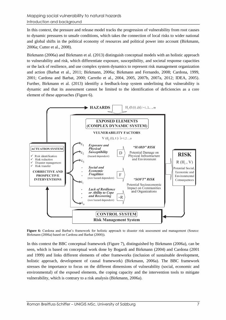
Further, Birkmann et al. (2013) identifiy a feedback-loop system underlining that vulnerability is
dynamic and that its assessment cannot be limited to the identification of deficiencies as a core
element of these approaches (Figure 6).
Figure 6: Cardona and Barbat’s framework for holistic approach to disaster risk assessment and management (Source:
Birkmann (2006a) based on Cardona and Barbat (2000)).
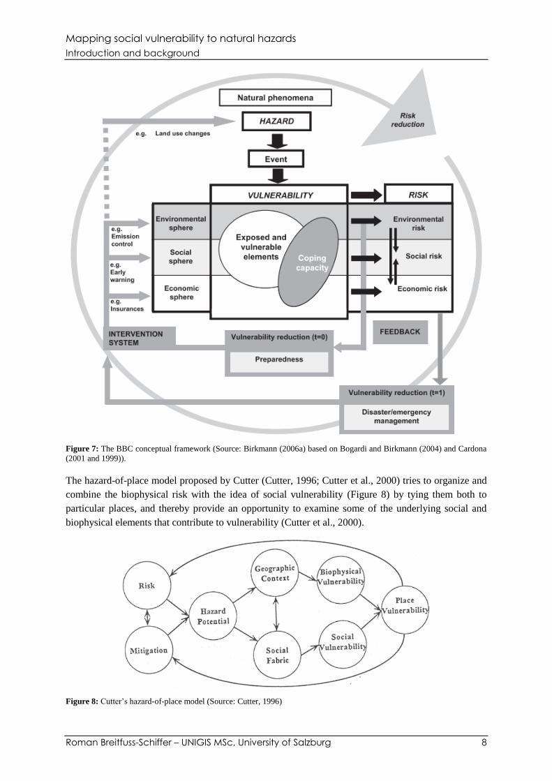
In this context the BBC conceptual framework (Figure 7), distinguished by Birkmann (2006a), can be
seen, which is based on conceptual work done by Bogardi and Birkmann (2004) and Cardona (2001
and 1999) and links different elements of other frameworks (inclusion of sustainable development,
holistic approach, development of causal framework) (Birkmann, 2006a). The BBC framework
stresses the importance to focus on the different dimensions of vulnerability (social, economic and
environmental) of the exposed elements, the coping capacity and the intervention tools to mitigate
vulnerability, which is contrary to a risk analysis (Birkmann, 2006a).
Mapping social vulnerability to natural hazards
Introduction and background
Roman Breitfuss-Schiffer – UNIGIS MSc, University of Salzburg 8
Figure 7: The BBC conceptual framework (Source: Birkmann (2006a) based on Bogardi and Birkmann (2004) and Cardona
(2001 and 1999)).
The hazard-of-place model proposed by Cutter (Cutter, 1996; Cutter et al., 2000) tries to organize and
combine the biophysical risk with the idea of social vulnerability (Figure 8) by tying them both to
particular places, and thereby provide an opportunity to examine some of the underlying social and
biophysical elements that contribute to vulnerability (Cutter et al., 2000).
Figure 8: Cutter’s hazard-of-place model (Source: Cutter, 1996)

Mapping social vulnerability to natural hazards
Introduction and background
Roman Breitfuss-Schiffer – UNIGIS MSc, University of Salzburg 9
In this model, risk and mitigation interact to produce a hazard potential, while the combination of
biophysical and social vulnerability creates the place vulnerability (Cutter, 1996; Cutter et al., 2000).
Birkmann et al. (2013) distinguish another school of thought within the context of climate change
adaptation research, in which most of the approaches focus on the definition of vulnerability used by
the IPCC, according to which vulnerability is seen as a function of exposure, sensitivity, and adaptive
capacities (Füssel, 2007b, 2007a; IPCC, 2007, 2001; G. O’Brien et al., 2008; K. O’Brien et al., 2008).
These approaches take the rate and magnitude of climate change into account when calculating the
vulnerability and therefore differ from the frameworks mentioned above (Birkmann et al., 2013).
Another holistic approach for assessing vulnerability is proposed by Birkmann et al. (2013) and is
called the MOVE framework (Figure 9) which was developed within the context of the research
project MOVE (Methods for the Improvement of Vulnerability Assessment in Europe) (Birkmann et
al., 2013). The intention of the framework was to encompass the multiple dimensions of vulnerability
by taking key factors into account such as exposure, susceptibility, lack of resilience (lack of societal
response capacities) as well as the different levels of vulnerability (physical, social, ecological,
economic, cultural, and institutional) (Birkmann et al., 2013). In addition, the concept of adaptation
into disaster risk management is included in the model (Birkmann et al., 2013).
Figure 9: The MOVE framework (Source: Birkmann et al. (2013) based on concepts of Birkmann, 2006a; Bogardi and
Birkmann, 2004; Cardona, 2001, 1999; Carreño et al., 2007a; IDEA, 2005; Turner et al., 2003).
Mapping social vulnerability to natural hazards
Introduction and background
Roman Breitfuss-Schiffer – UNIGIS MSc, University of Salzburg 10
1.2.2 Vulnerability indices
Within the above discussed conceptual frameworks by different authors, vulnerability is mostly
quantified by indicators, which are key tools for identifying and measuring vulnerability (Birkmann,
2006b). The importance of their development to enable decision-makers to assess the impact of
disasters was identified as a key activity by the international community on the World Conference on
Disaster Reduction (WCDR) in the year 2005 (UN, 2005).
The use of indicators to assess and describe certain phenomena such as the GDP to describe a state’s
economic performance or the Dow Jones to measure the development of the US stock market is
nowadays widely spread and commonly known. The development of social indicators emerged in the
1960s and 1970s (Cutter et al., 2003) followed by the development of environmental indicators in the
1970s connected to the formation of environmental policies (Birkmann, 2006b). The latest bigger
thematic complex regarding indicator development was research associated with sustainability
(Birkmann, 2006b).
Regarding social vulnerability, it is evident that this concept has multiple dimensions (Birkmann,
2006a; Miller et al., 2010; Villagran, 2006; Yoon, 2012), and therefore an adequate measure to
quantify the multidimensional facet of vulnerability would be some sort of composite index (Adger et
al., 2004; Barnett et al., 2008; Fatemi et al., 2017). Composite indicators are nowadays considered a
useful tool for policy analysis, public communication, and decision-making and the number of
indicators used is growing year after year (OECD, 2008), while Bandura (2008) lists nearly 180
composite indicators in existence around the world. However, as the concept of social vulnerability is
multidimensional (Birkmann, 2006a; Miller et al., 2010; Villagran, 2006; Yoon, 2012), the
development of indicators trying to quantify it will vary and therefore lead to the creation of different
indicators (Fatemi et al., 2017; Yoon, 2012). This, of course, has also to do with the fact that every
indicator is developed to serve a certain purpose (indicandum) and is related to certain goals
(Birkmann, 2006b). Furthermore, the process of indicator development should be underpinned by an
implicit conceptual model, which, of course, would influence the outcome of the corresponding
vulnerability indicator (Downing, 2004).
Indicators can be differentiated on many levels. While the essential function of indicators is basically
to quantify, an indicator could have either qualitative (nominal), ordinal (rank), or quantitative
characteristics (Gallopin, 1997). Furthermore, as an indicator should always be developed in relation
to a goal (Birkmann, 2006b), one can distinguish an indicator regarding its indicator-goal relations
(Weiland, 1999). On the one hand, an indicator can focus on the direction a development is taking,
which means that the development trend is used to evaluate e.g. vulnerability, while, on the other
hand, an indicator can focus on a specific target that shows whether the state or the development has
reached a defined value (Weiland, 1999). In addition, regarding social vulnerability Yoon (2012)
distinguishes between a deductive and an inductive method used for assessment. The deductive
approach, on the one hand, selects a limited number of variables to create a social vulnerability index
based on a priori theory and knowledge from existing literature, while the inductive approach, on the
other hand, includes all possible variables mentioned by literature and in a next step selects a set of
variables based on probabilistic or statistical relationships (Yoon, 2012).
When developing an index, there are certain guidelines, which can be helpful throughout the
development process. According to Maclaren (1996), ideally there are nine different phases (some of
which already mentioned above) in the development of indicators relating to urban sustainability,
which were applied to the development of vulnerability indicators by Birkmann (2006b, p.63).
Mapping social vulnerability to natural hazards
Introduction and background
Roman Breitfuss-Schiffer – UNIGIS MSc, University of Salzburg 11
1. Define goals: definition and selection of relevant goals
2. Scoping: identification of the target group and the associated purpose for which the indicators
will be used
3. Choose indicator framework: identification of the underlying conceptual framework
4. Define selection criteria: definition of selection criteria for the potential indicators to meet
certain defined standards in terms of viability and validity
5. Identify potential indicators: identification of a set of potential indicators, e.g. based on
existing vulnerability studies
6. Choose a final set of indicators: Evaluation of the indicators and selection of a final set in
regard of the defined selection criteria
7. Collect data & analyze indicator results: Collection of data for the chosen indicators to
evaluate the applicability of the approach
8. Prepare and present report
9. Assess indicator performance
The Organization for Economic Co-operation and Development (OECD) (2008) lists ten different
steps for building a composite indicator (OECD, 2008, p.20). While thematic overlaps do exist, those
steps do not fully correspond with the above-mentioned nine phases according to Maclaren (1996).
1. Theoretical framework: provides the basis for the selection and combination of variables into a
meaningful composite indicator
2. Data selection: should be based on analytical soundness, measurability, and relevance
3. Imputation of missing data: carried out in order to provide a complete dataset
4. Multivariate analysis: to study the overall structure of the dataset and derive subsequent
methodological choices
5. Normalization: to render the variables comparable
6. Weighting and aggregation: according to the underlying theoretical framework and the data
properties
7. Uncertainty and sensitivity analysis: to assess the robustness of the indicator in term of e.g. the
choice of weights, the imputation of missing data etc.
8. Back to the data: to reveal the main drivers for an overall good or bad performance
9. Links to other indicators: to identify correlation and regressions linked to other existing
indicators
10. Visualization of the results
It must be mentioned, that the nine phases according to Maclaren (1996) as well as the ten steps
suggested by the OECD (2008) have to be considered as “ideal process” or “ideal sequence”, which in
practice will be characterized by going back- and forwards (Birkmann, 2006b). Nevertheless, the
distinction between different steps or phases can be helpful regarding structuring the process of
indicator development as well as the analysis of current approaches and their development process
(Birkmann, 2006b).
1.3 Aims and objectives
Climate change is projected to increase risks from natural hazards such as heat stress, extreme
precipitation, inland flooding, or landslides for people in urban areas due to population growth and
poor planning and insufficient implementation of mitigation strategies (Pachauri et al., 2014).
Furthermore, Pachauri et al. (2014) point out that these risks are amplified for those people and
communities lacking essential infrastructure and services or living in exposed areas. Billions of people

Mapping social vulnerability to natural hazards
Introduction and background
Roman Breitfuss-Schiffer – UNIGIS MSc, University of Salzburg 12
are affected and threatened by natural and manmade disasters worldwide, while children are
disproportionally affected (International Federation of Red Cross and Red Crescent Societies, 2018;
SOS Children’s Villages International, 2017a; Wallemacq and Below, 2018). Supported by Allianz
SE, the Emergency Preparedness Program of the SOS Children’s Villages International seeks to tackle
these threats and challenges and aims to minimize weather- and conflict-related risks for local
communities (SOS Children’s Villages International, 2017a).
Within the context of the Emergency Preparedness Program, a project called RIVA (Risk and
Vulnerability Assessment) is conducted with the additional support of the Interfaculty Department of
Geoinformatics (Z_GIS) (SOS Children’s Villages International, 2017a). The main goal is to evaluate
and strengthen disaster preparedness and response capacities of local communities by developing
target trainings, closing communication gaps, and pre-positioning of vital resources (SOS Children’s
Villages International, 2017a). This assessment is carried out for ten different SOS Children’s Villages
worldwide (Allianz SE, 2017). While in a first step the assessment focuses on the SOS Children’s
Village itself, in a second step the assessment is extended to the surrounding area (SOS Children’s
Villages International, 2018). This findings will then be shared with local communities and NGOs
(Ruep, 2017).
Typically, the impacts and the magnitude of damage (physical, psychological etc.) due to natural
disasters are unevenly distributed among and within nations, regions, communities and groups of
individuals (Yoon, 2012). However, spatial modelling of vulnerability is not always regarded as a
central element (Kienberger et al., 2009) although vulnerability is strongly related to the specifics of a
place (place-based) (Cutter et al., 2008; November, 2008). Thus, based on the aims of RIVA, this
thesis focuses on the vulnerability of the inhabitants of the whole city of Quito in Ecuador in order to
get to a better understanding of the social vulnerability to natural hazards in urban areas. The
objectives are as follows:
(1) Quantification of the social vulnerability by developing a composite index based on a
theoretical risk and vulnerability framework
(2) Mapping of the social vulnerability for the city area of Quito (census block scale)
a. Revealing of hot and cold spots
b. Supporting tool for risk management
Mapping social vulnerability to natural hazards
Materials and methods
Roman Breitfuss-Schiffer – UNIGIS MSc, University of Salzburg 13
2. Materials and methods
2.1 Study area
When carrying out an assessment of vulnerability it is essential to stress that we can only talk
meaningfully about vulnerability of a specified system to a specified hazard or range of hazards
(Brooks, 2003). Therefore, it is of high importance to set the study area in proper relation to the
conducted vulnerability assessment study, as the conceptualization and the use of data or factors for
creating an index for the social vulnerability depends heavily on the study area and the context and
aim of the study carried out (de Loyola Hummell et al., 2016; Frigerio et al., 2016; Frigerio and De
Amicis, 2016).
As mentioned above (see 1.3), within the context of the RIVA project the assessment is carried out on
ten different SOS Children’s Villages and their surrounding area, while this thesis focuses on the
capital of Ecuador, the city of Quito (Figure 10 and Figure 11). This choice was made mainly since the
quality of the underlying data as well as the abundance of the data is better or higher compared to the
other case studies.
Figure 10: Location map of the city of Quito, Ecuador.
Figure 11: Map of the city and study area of Quito, Ecuador.
This thesis focuses on the assessment of social vulnerability in an urban area. While the metropolitan
district of Quito, which is located in the Pichincha Province, is much bigger than the city itself, the
study area is limited to the city of Quito and is related to the study area of the research study on
deprivation and healthcare accessibility by Cabrera-Barona et al. (2018), who made the according data
(e.g. shapefiles) available to the author. This approach also provides the possibility of a direct
comparison of the results, which could be interesting as deprivation might be related to social
vulnerability and show similar spatial patterns. The study area covers an area of around 195 km² with
around 1.6 million inhabitants according to the 2010 Ecuadorean Population and Housing Census.
The city of Quito is located in a mountain valley of high altitude (around 2,850 m above sea level) in
the northern part of Ecuador, close to the equator. The city is surrounded by several active and inactive
volcanoes.

Mapping social vulnerability to natural hazards
Materials and methods
Roman Breitfuss-Schiffer – UNIGIS MSc, University of Salzburg 14
2.1.1 SOS Children’s Village in Quito
SOS Children’s Villages International is providing supportive care when children can no longer live
with their families around the world (SOS Children’s Villages International, 2017b). Further, its aim is
to prevent family breakdown and to ensure that children’s rights are met by working with children,
families, communities and states (SOS Children’s Villages International, 2017b). Especially the family
strengthening programs help families to build capacities so that children are well cared for and
families can stay together (SOS Children’s Villages International, 2017b).
SOS Children’s Villages has been working in Quito since 1963, supporting over 1,200 people with the
family strengthening program throughout Quito (SOS Children’s Villages International, 2017b). In the
Children’s Village itself ten families with a total of 70 children found a new home, while 42 staff
members work in the village (SOS Children’s Villages International, 2018). The Children’s Village is
located in a populous area underlined by the fact that a total number of around 49,000 people are
living in the surrounding area (15 min walking time) (SOS Children’s Villages International, 2018).
Figure 12: Location of the SOS Children’s Village itself and other SOS CV premises in Quito. The district Quitumbe is
highlighted as it is considered for future extension by SOS CV.
In the first step of assessment in the course of the RIVA project it was found that the village itself is
highly exposed to volcanic hazards, while floods and new diseases (e.g. Zika, Chikungunya Fever)
where characterized as emerging hazards (SOS Children’s Villages International, 2018). Key
vulnerabilities were detected in the domain of coping capacity as well as regarding the capacity to
recover (SOS Children’s Villages International, 2018). Quitumbe, a district in the south of Quito, is
considered for further extension by SOS Children’s Villages in the future.
2.1.2 Natural hazards in Quito
Ecuador finds itself in one of the zones of highest tectonic complexity, resulting in high seismic and
volcanic activity (Municipio del Distrito Metropolitano de Quito, 2015). Additionally, it is located in
the Intertropical Convergence Zone and is therefore exposed to hazards of hydrometeorological origin
Mapping social vulnerability to natural hazards
Materials and methods
Roman Breitfuss-Schiffer – UNIGIS MSc, University of Salzburg 15
such as floods, droughts, storms and frosts (Municipio del Distrito Metropolitano de Quito, 2015).
Furthermore, due to the geomorphological conditions, processes of mass movement (e.g. landslides,
mud flows, erosion) are supported (Municipio del Distrito Metropolitano de Quito, 2015). Those
events of natural origin are periodically reoccurring throughout Ecuador, while Quito is no exception
(Municipio del Distrito Metropolitano de Quito, 2015). In principle, these hazards are of natural
origin, whereby, especially in the urban environment, human behavior, activities, and land use
influence physical processes (Municipio del Distrito Metropolitano de Quito, 2015). In addition,
climate change is projected to increase risks from natural hazards for people in urban areas due to
population growth and poor planning as well as insufficient implementation of mitigation strategies
(Pachauri et al., 2014).
Mass movements
Mass movements are displacements downhill from a mass of soil or rock whose movement occurs
predominantly along a slip or shear surface (Municipio del Distrito Metropolitano de Quito, 2015).
Those can be distinguished between the material type and the type of movement (Varnes, 1978). The
most common events developing in the area of the city of Quito are landslides generated in the
margins of the surrounding ravines, on the slopes of roads and on slopes generally steeper than 30° as
well as mud and debris flows (Municipio del Distrito Metropolitano de Quito, 2015). The intensity,
frequency, and occurrence of mass movement events are sometimes influenced by anthropogenic
interventions and actions such as deforestation, infrastructure installation, water infiltration due to
leaks in aqueducts and sewage systems, insufficiency of rainwater collection systems, and mining
(Municipio del Distrito Metropolitano de Quito, 2015). The exposure of the city center itself to
phenomena of mass movements is relatively low, while the threat is much higher in the outskirts in
proximity to the areas of higher elevation (Municipio del Distrito Metropolitano de Quito, 2015).
Floods
Rainfalls in Quito are characterized by spatial and temporal irregularities (Pourrut and Leiva, 1989),
and therefore strong, local rainfalls of short duration (rarely more than 1-2 hours) are leading to
flooding of the urban areas as well as alongside the courses of rivers (Municipio del Distrito
Metropolitano de Quito, 2015). Similar to the development of mass movements, flooding events are
influenced or even caused by anthropogenic interventions such as the sealing of the soil and the
insufficient rainwater collection systems, filling of natural drains, and deforestation (increasing runoff
in higher elevated areas of the watershed) (Municipio del Distrito Metropolitano de Quito, 2015). The
areas prone to flooding are more or less evenly distributed among the city area, while in the city center
the danger of flooding tends to be a little bit higher (Municipio del Distrito Metropolitano de Quito,
2015).
Volcanic hazards
Volcanic activity leads to phenomena with local, regional, and global effects and the history of
Ecuador is marked by several events of great magnitude causing environmental imbalances with
sometimes long-term consequences (Municipio del Distrito Metropolitano de Quito, 2015). Quito is
surrounded by several volcanoes such as the Guagua Pinchincha, Cotopaxi, Cayambe, Pululahua,
Ninahuilca, or El Reventador, which had seriously affected the city of Quito throughout history
(Municipio del Distrito Metropolitano de Quito, 2015). While pyroclastic flows are among the hazards
with a very high destructive force, the city of Quito faces very limited exposure to pyroclastic flows
(Municipio del Distrito Metropolitano de Quito, 2015). The city area is mostly exposed to ash fall and
Mapping social vulnerability to natural hazards
Materials and methods
Roman Breitfuss-Schiffer – UNIGIS MSc, University of Salzburg 16
flows of debris and mud (lahars), mostly caused by eruptions of Guagua Pichincha and Cotopaxi
located in the west and in the south-east, respectively (Municipio del Distrito Metropolitano de Quito,
2015).
Seismic hazards
Ecuador is a tectonically active country with high seismic activity due to being located in the
subduction zone of the Nazco oceanic plate under the continental plate of South America (Municipio
del Distrito Metropolitano de Quito, 2015). The magnitude of seismic vibrations at a certain point of
interest depends on several factors, such as the magnitude of the earthquake, the distance from the
fault (fracture), and the “local effect”, which depends on soil types and thickness, relief, and
topography (Municipio del Distrito Metropolitano de Quito, 2015). Crossed by a fault system, the city
of Quito is located in an area of high seismic activity and has been affected by many intense
earthquakes throughout history (Municipio del Distrito Metropolitano de Quito, 2015). Seismic micro
zoning assessment studies show that the city center as well as the southern part of the city are exposed
to a higher seismic hazard than the northern part of the city (Municipio del Distrito Metropolitano de
Quito, 2015).
Forest fires
Forest fires bear a high destructive force, as their outbreak results in loss of infrastructure and
environmental deterioration to a high degree (Municipio del Distrito Metropolitano de Quito, 2015).
The inflammability and combustibility play an important role regarding the susceptibility to forest
fires, while it is also influenced by other factors, such as e.g. accessibility (Municipio del Distrito
Metropolitano de Quito, 2015). In the city of Quito itself, only a few areas are susceptible to forest
fires, e.g. the forest running north-south in the central part of the district and forests in eastern parts of
the city (Municipio del Distrito Metropolitano de Quito, 2015).
Solar radiation
Throughout the last couple of years, reports on very high solar (ultraviolet) radiation in whole Ecuador
and in the city area of Quito itself became more frequent and the exposure to it is considered a serious
health threat (CuencaHighLife, 2017; El Comercio, 2018; Parra et al., 2018; Serrano et al., 2014).
Nevertheless, this hazard will not be considered in the indicator selection process.
2.2 Underlying data
2.2.1 Census data 2010
The 2010 Ecuadorean Population and Housing Census provides the socio-economic data for the
creation of a social vulnerability index. The Population and Housing Census is carried out by the
National Institute of Statistics and Censuses (Instituto Nacional de Estadisticas y Censos – INEC). The
first census was carried out in 1950, while the last one was carried out in the year 2010 (INEC, 2014).
The data is publicly available for free on the website of the National Institute of Statistics and
Censuses at http://www.ecuadorencifras.gob.ec/censo-de-poblacion-y-vivienda (accessed on
31/08/2018).
2.2.2 Hazard data
There are two types of data available describing the different hazards in the study area: data of
hazardous events and data describing the danger facing different types of hazards. As this thesis
Mapping social vulnerability to natural hazards
Materials and methods
Roman Breitfuss-Schiffer – UNIGIS MSc, University of Salzburg 17
focuses on the assessment of social vulnerability only and not on the exposure to natural hazards (see
2.3), the hazard data will not be included in the assessment itself. Nevertheless, this data might be
useful in terms of visualization and interpretation of this thesis’ results. This data is publicly available
for free on the Quito Open Data website at http://gobiernoabierto.quito.gob.ec/?page_id=1105 and at
http://geo.quito.gob.ec:8080/geoserver/web/?wicket:bookmarkablePage=:org.geoserver.web.demo.Ma
pPreviewPage (accessed on 17/09/2018) in the shape file format.
Data of hazardous events
Point data represents different hazardous events i.e. floods and mass movements from 2005 to 2017.
Data of danger facing natural hazards
The danger facing natural hazards is represented by polygons referring to certain levels of danger
facing mass movements, floods, volcanic hazards and forest fires.
2.2.3 Other data
Deprivation index, Healthcare accessibility
The results of the study regarding deprivation and healthcare accessibility of Cabrera-Barona et al.
(2018) were made available to the author by Pablo Cabrera-Barona in the shape file format.
Data associated with the RIVA project
Various data associated with the ongoing RIVA project (see 1.3) and the assessment carried out in the
first level of the project was provided by Stefan Kienberger. This data includes i.a. point data of
different amenities (e.g. SOS CV, healthcare services, educational services, public transportation,
security), line data of the street network, and line data of major and minor rivers. This data might be
useful in terms of the interpretation of this thesis’ results and their visualization but will not be
included in the social vulnerability assessment itself.
In addition, the data includes point data of hazard events and polygon data of the danger facing
volcanic hazards and mass movements. This data is mainly consistent with the above-mentioned data
(2.2.2).
2.3 Conceptual framework
When carrying out a vulnerability assessment the underlying conceptual framework is of high
importance, as it incorporates a certain vulnerability definition and therefore influences the
development process of the corresponding vulnerability index (Downing, 2004; Maclaren, 1996;
OECD, 2008). An overview of different vulnerability definitions and conceptual frameworks was
given in chapter 1.1.1..
The underlying conceptual framework for the first level of vulnerability assessment regarding the
RIVA project was the MOVE framework established by Birkmann et al. (2013). As this thesis is
conducted in relation to the RIVA project, the same conceptual framework will be applied.
The framework has been developed within the context of the research project MOVE (Methods for the
Improvement of Vulnerability Assessment in Europe) and is underlined by a multi-dimensional and
holistic approach to vulnerability assessment that is understood as part of risk evaluation and risk
management in the context of disaster risk management (DRM) and climate change adaptation (CCA)

Mapping social vulnerability to natural hazards
Materials and methods
Roman Breitfuss-Schiffer – UNIGIS MSc, University of Salzburg 18
(Birkmann et al., 2013). As already elaborated above, this thesis focuses specifically on the
vulnerability domain of the framework and its social dimension only. Therefore, the exposure domain
is excluded from the assessment as the potentiality of harm is independent from a hazard delineation,
which is based on certain model assumptions with related uncertainties (Kienberger et al., 2014).
Thus, this assessment will focus on localizing potential vulnerable areas based on their predispositions
and general characteristics regarding the social dimension (Kienberger et al., 2014). Further, the
subdomains of the “lack of resilience” domain were relabeled in the sense that the domain is coherent
with the negative association regarding vulnerability (Kienberger et al., 2014). As already mentioned
above (see 2.1), the study area is the city of Quito, which would relate to a subnational to local scale
regarding the framework. The adapted framework is depicted in Figure 13.
Figure 13: Adapted MOVE risk and vulnerability framework based on Birkmann et al. (2013) – The assessment is carried
out on a subnational to local scale. The relevant domains are highlighted, while the exposure domain is excluded from the
assessment.
Besides the key causal factors (exposure, susceptibility, lack of resilience), the MOVE framework
incorporates different thematic dimensions of vulnerability such as physical, social, ecological,
economic, cultural, and institutional dimensions (Birkmann et al., 2013). The social dimension of
vulnerability within the framework is described as “propensity for human well-being to be damaged
by disruption to individual (mental and physical health) and collective (health, education services, etc.)
social systems and their characteristics (e.g. gender, marginalization of social groups) (Birkmann et
al., 2013, p.200).”
Additionally, a core element of the underlying framework is the incorporation of a feedback-loop
system (risk governance, adaptation) underlining that vulnerability and risk are part of various
processes of a dynamic nature and therefore change over time (Birkmann et al., 2013).
Mapping social vulnerability to natural hazards
Materials and methods
Roman Breitfuss-Schiffer – UNIGIS MSc, University of Salzburg 19
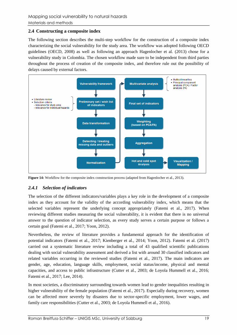
2.4 Constructing a composite index
The following section describes the multi-step workflow for the construction of a composite index
characterizing the social vulnerability for the study area. The workflow was adopted following OECD
guidelines (OECD, 2008) as well as following an approach Hagenlocher et al. (2013) chose for a
vulnerability study in Colombia. The chosen workflow made sure to be independent from third parties
throughout the process of creation of the composite index, and therefore rule out the possibility of
delays caused by external factors.
Figure 14: Workflow for the composite index construction process (adapted from Hagenlocher et al., 2013).
2.4.1 Selection of indicators
The selection of the different indicators/variables plays a key role in the development of a composite
index as they account for the validity of the according vulnerability index, which means that the
selected variables represent the underlying concept appropriately (Fatemi et al., 2017). When
reviewing different studies measuring the social vulnerability, it is evident that there is no universal
answer to the question of indicator selection, as every study serves a certain purpose or follows a
certain goal (Fatemi et al., 2017; Yoon, 2012).
Nevertheless, the review of literature provides a fundamental approach for the identification of
potential indicators (Fatemi et al., 2017; Kienberger et al., 2014; Yoon, 2012). Fatemi et al. (2017)
carried out a systematic literature review including a total of 43 qualified scientific publications
dealing with social vulnerability assessment and derived a list with around 30 classified indicators and
related variables occurring in the reviewed studies (Fatemi et al., 2017). The main indicators are
gender, age, education, language skills, employment, social status/income, physical and mental
capacities, and access to public infrastructure (Cutter et al., 2003; de Loyola Hummell et al., 2016;
Fatemi et al., 2017; Lee, 2014).
In most societies, a discriminatory surrounding towards women lead to gender inequalities resulting in
higher vulnerability of the female population (Fatemi et al., 2017). Especially during recovery, women
can be affected more severely by disasters due to sector-specific employment, lower wages, and
family care responsibilities (Cutter et al., 2003; de Loyola Hummell et al., 2016).
Mapping social vulnerability to natural hazards
Materials and methods
Roman Breitfuss-Schiffer – UNIGIS MSc, University of Salzburg 20
Furthermore, the distribution of age groups in a society have an impact on the vulnerability. Especially
extremes in the age spectrum may increase social vulnerability, as children and elders are dependent
on others in terms of financial and physical support, in particular during and after disasters (Cutter et
al., 2003; Fatemi et al., 2017; Kienberger et al., 2014).
Higher education is often linked to lower vulnerability because people with higher education have
better access to resources (e.g. financial) and have a higher capability of accessing and understanding
warning or recovery information (Cutter et al., 2003; Fatemi et al., 2017).
Immigration and the related social vulnerability is a widely discussed issue. Cutter et al. (2003) argue
that language and cultural barriers could affect the access to financial help or funding in the post-
disaster phase. Furthermore, immigrants, especially those who have recently moved to a new city,
have less experience and knowledge regarding the local types of natural hazards leading to possibly
wrong reactions during the disaster (de Loyola Hummell et al., 2016).
Employment and socio-economic status are related in most societies. The fact of being unemployed or
being subjected to poverty may increase the social vulnerability as the ability to absorb losses and
recover from disasters may decrease, while, on the contrary, wealth enables communities to deal with
and recover from natural hazards more quickly (Cutter et al., 2003; de Loyola Hummell et al., 2016).
Also, being employed in different sectors may lead to different levels of social vulnerabilities as
sectors may be differentially affected by disasters (Kienberger et al., 2014). For instance, societies that
are heavily dependent on agriculture, tourism-related activities, or extractive industries might be more
vulnerable compared to others, while a strong public employment sector might decrease social
vulnerability (Cutter et al., 2003; de Loyola Hummell et al., 2016; Kienberger et al., 2014).
Population with special needs (e.g. physically or mentally handicapped) are highly vulnerable and can
be heavily affected by disaster, as they require special attention or infrastructure during a hazardous
event, but also in the post-disaster phase (Cutter et al., 2003; de Loyola Hummell et al., 2016).
Especially people residing in group quarters (e.g. nursing homes) have a particular vulnerability
(Fatemi et al., 2017).
Accessibility of households to public infrastructures such as roads, water supply, electricity are of high
importance regarding the social vulnerability (Cutter et al., 2003; Fatemi et al., 2017; Kienberger et
al., 2014). Furthermore, the access to public services like early warning systems and healthcare
infrastructure affect the level of social vulnerability (Fatemi et al., 2017; Kienberger et al., 2014).
As a first step, potential vulnerability indicators were identified from scientific publications (Cabrera-
Barona et al., 2018; Cutter et al., 2003; de Loyola Hummell et al., 2016; Fatemi et al., 2017;
Kienberger et al., 2014), while the main criteria to select the indicators were the relevance for the
study area as well as the relevance for the individual hazards (Kienberger et al., 2014). The selection
process led to a preliminary set or a wish list of indicators (Table 1) describing the social dimension of
vulnerability in the study area to the natural hazards listed in chapter 2.1.2, excluding solar radiation.
According to the adapted MOVE framework (Figure 13), the variables were assigned either to the lack
of resilience (LoR) or the susceptibility (SUS) domain. Furthermore, a positive (+) or negative (-) sign
indicates whether the social vulnerability increases or decreases with a higher value. This set of
indicators is characterized as preliminary or as wish list because the availability of actual data to
represent the individual indicators was not yet included in the selection process.

Mapping social vulnerability to natural hazards
Materials and methods
Roman Breitfuss-Schiffer – UNIGIS MSc, University of Salzburg 21
Table 1: Preliminary set/wish list of indicators with the according variables and domain (SUS – Susceptibility, LoR – Lack
of Resilience). Sign indicates if a higher value increases (+) or decreases (-) vulnerability.
Nr. Indicator Variable Domain Sign
1.1 Female population Percentage of females LoR +
1.2 Percentage of female headed households LoR +
1.3 Percentage of employed females in the labor force LoR +
2.1 Age structure Median age SUS +
2.2 Percentage <5 years old SUS +
2.3 Percentage >64 years old SUS +
3.1 Family structure Average number of people per household SUS +
3.2 Percentage of households with four or more persons per dormitory SUS +
4.1 Population characteristics Population density SUS +
5.1 Race/Ethnicity & Minorities Percent of minorities (e.g. indigenous people) LoR +
5.2 Percentage of population born in other states LoR +
5.3 Percentage of residents immigrating in the past 3-5 years LoR +
6.1 Quality of built environment Percentage of households with no water infrastructure or well LoR +
6.2 Percentage of households with no sewer infrastructure LoR +
6.3 Percentage of households with no garbage collection services LoR +
6.4 Percentage of households with no electricity service LoR +
6.5 Percentage of population living in households with low quality
external walls
LoR +
6.6 Percentage of population living in households with low quality
roofs
LoR +
7.1 Housing unit status Percentage of population living in rented households LoR +
8.1 Socioeconomic
status/Income
Percentage of households with no phone (cell phone or landline) LoR +
8.2 Percentage of population living in households facing extreme
poverty
LoR +
8.3 Per capita income LoR -
9.1 Education Percentage of illiterate population aged 15 and older LoR +
9.2 Percentage of population that completed middle school or with high
school incomplete
LoR -
9.3 Percentage of population that completed college degree LoR -
9.4
Percentage of population with no level of formal education or
instruction
LoR +
10.1 Employment Percentage of population unemployed SUS +
10.2 Percentage of population employed in agriculture, mining, forestry
production, livestock, and aquaculture
SUS +
10.3 Percentage of population employed in extractive industry SUS +
10.4 Percentage of population employed in accommodation activities SUS +
10.5 Percentage of population employed in food service activities SUS +
10.6 Percentage of population employed in commerce SUS +
10.7 Percentage of population employed in public administration,
defense and social security
SUS -
10.8 Percentage of population employed in human health and social
work services
LoR -
10.9 Percentage of population that works in unpaid jobs LoR +
11.1 Occupation Percentage of labor force with legal work registration LoR -
11.2 Percentage of labor force with no legal work registration LoR +
11.3 Percentage of subsistence workers in the labor force LoR +
12.1 Special needs population Percentage of population with at least one type of deficiency SUS +
13.1 Healthcare accessibility Index of Healthcare Accessibility (Cabrera-Barona et al., 2018) LoR -
Mapping social vulnerability to natural hazards
Materials and methods
Roman Breitfuss-Schiffer – UNIGIS MSc, University of Salzburg 22
Table 1 (continued)
Nr. Indicator Variable Domain Sign
14.1 Access to roads
LoR -
15.1 Early warning systems LoR -
2.4.2 Data transformation
The raw data of the 2010 Ecuadorean Population and Housing Census was downloaded in the
REDATAM format and the desired census variables were extracted for the study area with the freely
available software Redatam 7 (https://www.cepal.org/en/topics/redatam/download-redatam, accessed
on 29/01/2019). The data extraction was based on a geographical selection criterion representing the
study area (city of Quito) on the level of census blocks, while two census blocks, where no census data
was available,e were excluded. The census raw data was used to calculate most of the variables, while
the data was transformed to render the variables better comparable. Hence, nearly all variables
represent relative values in relation to the according subgroup of the population, the total numbers of
households or the census block area. For example, the percentage of unemployed individuals was
calculated in relation to the working population (i.e. excluding children, retired individuals etc.). the
only variable not expressed as relative value is the median age. Due to unavailable representative data,
some variables listed in Table 1 had to be dropped (8.2, 8.3, 9.2, 11.1, 11.2, and 15.1) and two
variables had to be merged together (10.4 and 10.5). Detailed information about the calculation of the
variables can be found in Appendix A.
As mentioned above (see 2.2.3), data of the study regarding deprivation and healthcare accessibility in
the city of Quito of Cabrera-Barona et al. (2018) where made available to the Author by Pablo
Cabrera-Barona. Thus, the healthcare accessibility data was included in the assessment of social
vulnerability.
Data and statistical analysis were carried out using the software RStudio as well as Microsoft Excel.
The script used in RStudio can be found in Appendix B.
2.4.3 Missing data and outliers
Descriptive statistical analysis was carried out to describe each variable. Following relevant literature
(Groeneveld and Meeden, 1984; Hagenlocher et al., 2013; Saisana, 2012), variables with skewness
> 2.0 and kurtosis (excess) > 3.5 were highlighted as statistically problematic with regard to potential
outliers. These variables are listed in Table 2. To calculate the skewness and kurtosis in R the package
moments was used.
In general, it is important to examine extreme values as they can become unintended benchmarks and
further may influence subsequent steps in the process of building a composite indicator (OECD,
2008). One common way of treating outliers would be by limiting the variable distribution to certain
percentile scores (e.g. 2.5 and 97.5) and winsorizing the data outside those limits accordingly (OECD,
2008; Saisana, 2012). Furthermore, transformations (e.g. logarithmic transformation) are widely
spread to reduce the skewness of highly skewed data, while it should be kept in mind that the
transformation would effect subsequent steps (e.g. normalization, aggregation) in the process of
building a composite indicator (OECD, 2008; Saisana, 2012). It was decided to include variable 10.3
and 14.1 into the model without further treatment, as the skewness is exceeded only to a very small
extent.
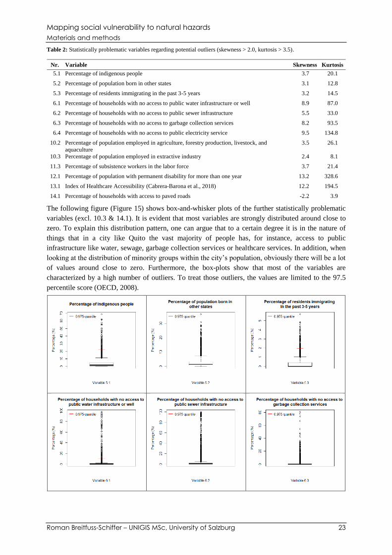
Mapping social vulnerability to natural hazards
Materials and methods
Roman Breitfuss-Schiffer – UNIGIS MSc, University of Salzburg 23
Table 2: Statistically problematic variables regarding potential outliers (skewness > 2.0, kurtosis > 3.5).
Nr. Variable Skewness Kurtosis
5.1 Percentage of indigenous people 3.7 20.1
5.2 Percentage of population born in other states 3.1 12.8
5.3 Percentage of residents immigrating in the past 3-5 years 3.2 14.5
6.1 Percentage of households with no access to public water infrastructure or well 8.9 87.0
6.2 Percentage of households with no access to public sewer infrastructure 5.5 33.0
6.3 Percentage of households with no access to garbage collection services 8.2 93.5
6.4 Percentage of households with no access to public electricity service 9.5 134.8
10.2 Percentage of population employed in agriculture, forestry production, livestock, and
aquaculture
3.5 26.1
10.3 Percentage of population employed in extractive industry 2.4 8.1
11.3 Percentage of subsistence workers in the labor force 3.7 21.4
12.1 Percentage of population with permanent disability for more than one year 13.2 328.6
13.1 Index of Healthcare Accessibility (Cabrera-Barona et al., 2018) 12.2 194.5
14.1 Percentage of households with access to paved roads -2.2 3.9
The following figure (Figure 15) shows box-and-whisker plots of the further statistically problematic
variables (excl. 10.3 & 14.1). It is evident that most variables are strongly distributed around close to
zero. To explain this distribution pattern, one can argue that to a certain degree it is in the nature of
things that in a city like Quito the vast majority of people has, for instance, access to public
infrastructure like water, sewage, garbage collection services or healthcare services. In addition, when
looking at the distribution of minority groups within the city’s population, obviously there will be a lot
of values around close to zero. Furthermore, the box-plots show that most of the variables are
characterized by a high number of outliers. To treat those outliers, the values are limited to the 97.5
percentile score (OECD, 2008).
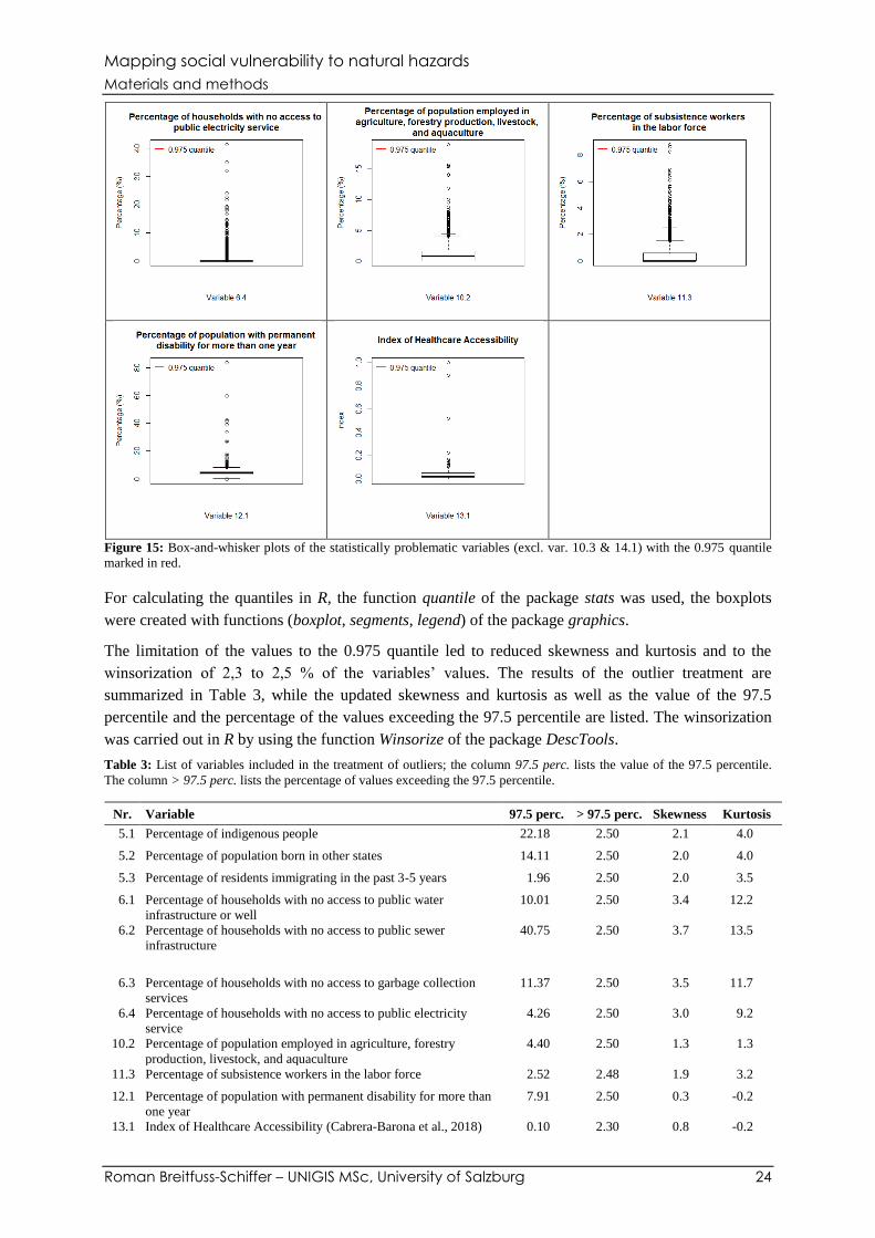
Mapping social vulnerability to natural hazards
Materials and methods
Roman Breitfuss-Schiffer – UNIGIS MSc, University of Salzburg 24
Figure 15: Box-and-whisker plots of the statistically problematic variables (excl. var. 10.3 & 14.1) with the 0.975 quantile
marked in red.
For calculating the quantiles in R, the function quantile of the package stats was used, the boxplots
were created with functions (boxplot, segments, legend) of the package graphics.
The limitation of the values to the 0.975 quantile led to reduced skewness and kurtosis and to the
winsorization of 2,3 to 2,5 % of the variables’ values. The results of the outlier treatment are
summarized in Table 3, while the updated skewness and kurtosis as well as the value of the 97.5
percentile and the percentage of the values exceeding the 97.5 percentile are listed. The winsorization
was carried out in R by using the function Winsorize of the package DescTools.
Table 3: List of variables included in the treatment of outliers; the column 97.5 perc. lists the value of the 97.5 percentile.
The column > 97.5 perc. lists the percentage of values exceeding the 97.5 percentile.
Nr. Variable 97.5 perc. > 97.5 perc. Skewness Kurtosis
5.1 Percentage of indigenous people 22.18 2.50 2.1 4.0
5.2 Percentage of population born in other states 14.11 2.50 2.0 4.0
5.3 Percentage of residents immigrating in the past 3-5 years 1.96 2.50 2.0 3.5
6.1 Percentage of households with no access to public water
infrastructure or well
10.01 2.50 3.4 12.2
6.2 Percentage of households with no access to public sewer
infrastructure
40.75 2.50 3.7 13.5
6.3 Percentage of households with no access to garbage collection
services
11.37 2.50 3.5 11.7
6.4 Percentage of households with no access to public electricity
service
4.26 2.50 3.0 9.2
10.2 Percentage of population employed in agriculture, forestry
production, livestock, and aquaculture
4.40 2.50 1.3 1.3
11.3 Percentage of subsistence workers in the labor force 2.52 2.48 1.9 3.2
12.1 Percentage of population with permanent disability for more than
one year
7.91 2.50 0.3 -0.2
13.1 Index of Healthcare Accessibility (Cabrera-Barona et al., 2018) 0.10 2.30 0.8 -0.2

Mapping social vulnerability to natural hazards
Materials and methods
Roman Breitfuss-Schiffer – UNIGIS MSc, University of Salzburg 25
As the values of the skewness and kurtosis were decreased to an acceptable degree, the variables were
included in the subsequent steps of the creation of the composite index.
No missing data was detected, as the census blocks with no available census data were already
excluded in the geographical selection (see 2.4.2).
2.4.4 Normalization
To render the variables comparable, all variables were standardized using linear min-max
normalization (equation 1) and z-score standardization (equation 2).
The min-max normalization results in values between 0 and 1 (OECD, 2008). Therefore, min-max
normalization facilitates the aggregation of the variables to a composite indicator (Hagenlocher et al.,
2013) and hence, was chosen as normalization method. However, it should be kept in mind that
extreme values (or outliers) could distort the transformed variable (OECD, 2008).
𝑣𝑖′ =(𝑣𝑖 − 𝑣𝑚𝑖𝑛)
(𝑣𝑚𝑎𝑥 − 𝑣𝑚𝑖𝑛)∗ 𝑠𝑖𝑔𝑛 + 0.5 ∗ (1 − 𝑠𝑖𝑔𝑛) (1)
𝑣𝑖’ normalized value
𝑣𝑖 actual value
𝑣𝑚𝑖𝑛 minimal value of variable distribution
𝑣𝑚𝑎𝑥 maximal value of variable distribution
𝑠𝑖𝑔𝑛 indication if variable contributes positively or negatively to vulnerability
Z-score standardization converts variables to a common scale with a mean of zero and standard
deviation of one (OECD, 2008). Z-scores standardization values were calculated additionally as they
are useful for subsequent statistical analysis (e.g. principal component analysis or factor analysis)
(Hagenlocher et al., 2013).
𝑣𝑖′′ =(𝑣𝑖 − �̅�)
𝜎∗ 𝑠𝑖𝑔𝑛 (2)
𝑣𝑖’’ standardized value
𝑣𝑖 actual value
�̅� mean value of the data
σ maximal value of variable distribution
𝑠𝑖𝑔𝑛 indication if variable contributes positively or negatively to vulnerability
The min-max normalization and the z-score standardization were carried out in R by using the function
normalise_ci of the package Compind.
2.4.5 Multivariate analysis
Multivariate analysis refers to any simultaneous analysis of more than two variables (Hair et al.,
2010). More precisely, to be considered truly multivariate, all the variables must be interrelated in
such ways that their different effects cannot meaningfully be interpreted separately (Hair et al., 2010).
It aims to measure, explain and predict the degree of relationships among the variates (weighted
combinations of variables) in the model (Hair et al., 2010).
Highly collinear variables within a domain (SUS, LoR) need to be detected and treated to ultimately
reduce overall multicollinearities within the data, as they would influence principal component
analysis and the overall output of the composite indicator (Hagenlocher et al., 2013; OECD, 2008;
Saisana, 2012). Pearson’s r as well as VIF (variance inflation factor) values were calculated for each

Mapping social vulnerability to natural hazards
Materials and methods
Roman Breitfuss-Schiffer – UNIGIS MSc, University of Salzburg 26
domain separately to exclude variables based on thresholds (r > 0.8, VIF > 5.0) (Hagenlocher et al.,
2013; OECD, 2008; Saisana, 2012). Figure 16 and Table 4 give an overview of the calculated r and
VIF values. Table 5 lists variables with critical values regarding the above-mentioned thresholds in
terms of high collinearity. The values for Pearson’s r were calculated in R using the function cor in the
package stats while the visualization of the correlation matrices was created using the function
corrplot of the package with the same name.
Figure 16: Visualization of correlation matrices with values of Pearson’s r for each of the two vulnerability domains (SUS –
left, LoR – right).
Table 4: VIF values for each variable of the two vulnerability domains.
SUS
Var.
Nr. 2.1 2.2 2.3 3.1 3.2 4.1 10.1 10.2 10.3 10.4 10.5 10.6 10.7 12.1
VIF 8.0 2.5 4.1 2.3 2.5 1.2 1.1 1.2 1.3 1.1 1.1 1.6 1.6 1.2
LoR
Var.
Nr. 1.1 1.2 1.3 5.1 5.2 5.3 6.1 6.2 6.3 6.4 6.5 6.6 7.1 8.1 9.1 9.3 9.4 10.8 11.3 13.1 14.1
VIF 1.7 1.7 2.6 1.8 3.3 1.9 1.7 2.5 2.3 1.6 2.1 2.4 1.6 2.5 6.4 5.3 5.2 1.1 1.2 1.1 2.3

Mapping social vulnerability to natural hazards
Materials and methods
Roman Breitfuss-Schiffer – UNIGIS MSc, University of Salzburg 27
Table 5: Variables with critical values of high collinearity based on thresholds for Pearson’s r and/or VIF.
Nr. Variable Pearson’s r (2nd variable) VIF
SUS
2.1 Median age 0.83 (2.3) 8.0
2.3 Percentage >64 years old 0.83 (2.1) 4.1
LoR
9.1 Percentage of illiterate population aged 15 and older 0.89 (9.4) 6.4
9.3 Percentage of population that completed college degree -0.73 (5.2) 5.3
9.4 Percentage of population with no level of formal education or instruction 0.89 (9.1) 5.2
For the calculation of VIF values in R, a linear model (function lm, package stats) within each of the
two domains was fitted to a matrix containing variables of the same values. The actual VIF values
were calculated using the function vif contained in the package car.
To reduce collinearity between the variables, the variable 2.1 (Median age) and 9.1 (Percentage of
illiterate population aged 15 and older) were eliminated. This decision was based on the respective
correlation matrix and the VIF values of the according variables. After elimination, the VIF of variable
2.3 and 9.4 dropped to 2.3 and 2.6, respectively. The VIF of variable 9.3 (Percentage of population
that completed college degree) dropped to 5.2, still exceeding the threshold of 5.0. Hence, the variable
9.3 was as well eliminated.
As mentioned above (Figure 14), the weighting of the components of the composite indicator will be
based on weights derived from principal component analysis (PCA) and factor analysis (FA) to be
independent from third parties, and therefore rule out the possibility of delays caused by external
factors. Therefore, PCA and FA were conducted within each of the two domains to prepare the data
for subsequent steps. Prior to PCA and FA, the data was normalized using z-score standardization, as
regarding PCA, it helps to prevent one variable having an undue influence on the principal
components and, regarding FA the normalization is required anyway (OECD, 2008).
The objective of PCA is to explain the variance of the observed data through a few linear
combinations of the original data, which are uncorrelated and called principal components, and to
select those principal components that represent a high amount of the overall variance of the original
data (OECD, 2008). FA is similar to PCA, as it also aims to describe the original data with a smaller
number of factors by highlighting the relationship between those factors (OECD, 2008). The question
of how many factors should be kept in the model for further analysis without losing too much
information is of high importance, while the most common method is PCA to extract the first principal
components and to consider them as factors (OECD, 2008). For FA only a subset of principal
components which account for the majority of the variance is retained and they are identified based on
certain criteria (OECD, 2008). The most common standard practice is to choose factors that (OECD,
2008, p.89)
- have associated eigenvalues larger than one (Kaiser criterion),
- contribute individually to the explanation of overall variance by more than 10%,
- contribute cumulatively to the explanation of the overall variance by more than 60%.
An eigenvalue smaller one would mean that the according factor would explain less variance than is
contained in one individual variable (OECD, 2008).
The results of the PCA for each of the two domains are summarized in Table 6, listing the eigenvalues
with the according variance. In the SUS domain, the first principal component explains 29.0 % of the
variance in all the variables (eigenvalue of 3.8), while the second principal component accounts for
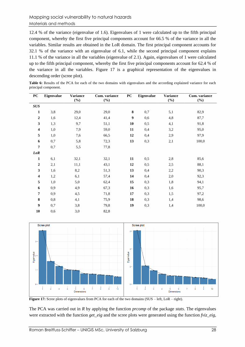
Mapping social vulnerability to natural hazards
Materials and methods
Roman Breitfuss-Schiffer – UNIGIS MSc, University of Salzburg 28
12.4 % of the variance (eigenvalue of 1.6). Eigenvalues of 1 were calculated up to the fifth principal
component, whereby the first five principal components account for 66.5 % of the variance in all the
variables. Similar results are obtained in the LoR domain. The first principal component accounts for
32.1 % of the variance with an eigenvalue of 6.1, while the second principal component explains
11.1 % of the variance in all the variables (eigenvalue of 2.1). Again, eigenvalues of 1 were calculated
up to the fifth principal component, whereby the first five principal components account for 62.4 % of
the variance in all the variables. Figure 17 is a graphical representation of the eigenvalues in
descending order (scree plot).
Table 6: Results of the PCA for each of the two domains with eigenvalues and the according explained variance for each
principal component.
PC Eigenvalue Variance
(%)
Cum. variance
(%)
PC Eigenvalue Variance
(%)
Cum. variance
(%)
SUS
1 3,8 29,0 29,0 8 0,7 5,1 82,9
2 1,6 12,4 41,4 9 0,6 4,8 87,7
3 1,3 9,7 51,1 10 0,5 4,1 91,8
4 1,0 7,9 59,0 11 0,4 3,2 95,0
5 1,0 7,6 66,5 12 0,4 2,9 97,9
6 0,7 5,8 72,3 13 0,3 2,1 100,0
7 0,7 5,5 77,8
LoR
1 6,1 32,1 32,1 11 0,5 2,8 85,6
2 2,1 11,1 43,1 12 0,5 2,5 88,1
3 1,6 8,2 51,3 13 0,4 2,2 90,3
4 1,2 6,1 57,4 14 0,4 2,0 92,3
5 1,0 5,0 62,4 15 0,3 1,8 94,1
6 0,9 4,9 67,3 16 0,3 1,6 95,7
7 0,9 4,5 71,8 17 0,3 1,5 97,2
8 0,8 4,1 75,9 18 0,3 1,4 98,6
9 0,7 3,8 79,8 19 0,3 1,4 100,0
10 0,6 3,0 82,8
Figure 17: Scree plots of eigenvalues from PCA for each of the two domains (SUS – left, LoR – right).
The PCA was carried out in R by applying the function prcomp of the package stats. The eigenvalues
were extracted with the function get_eig and the scree plots were generated using the function fviz_eig,
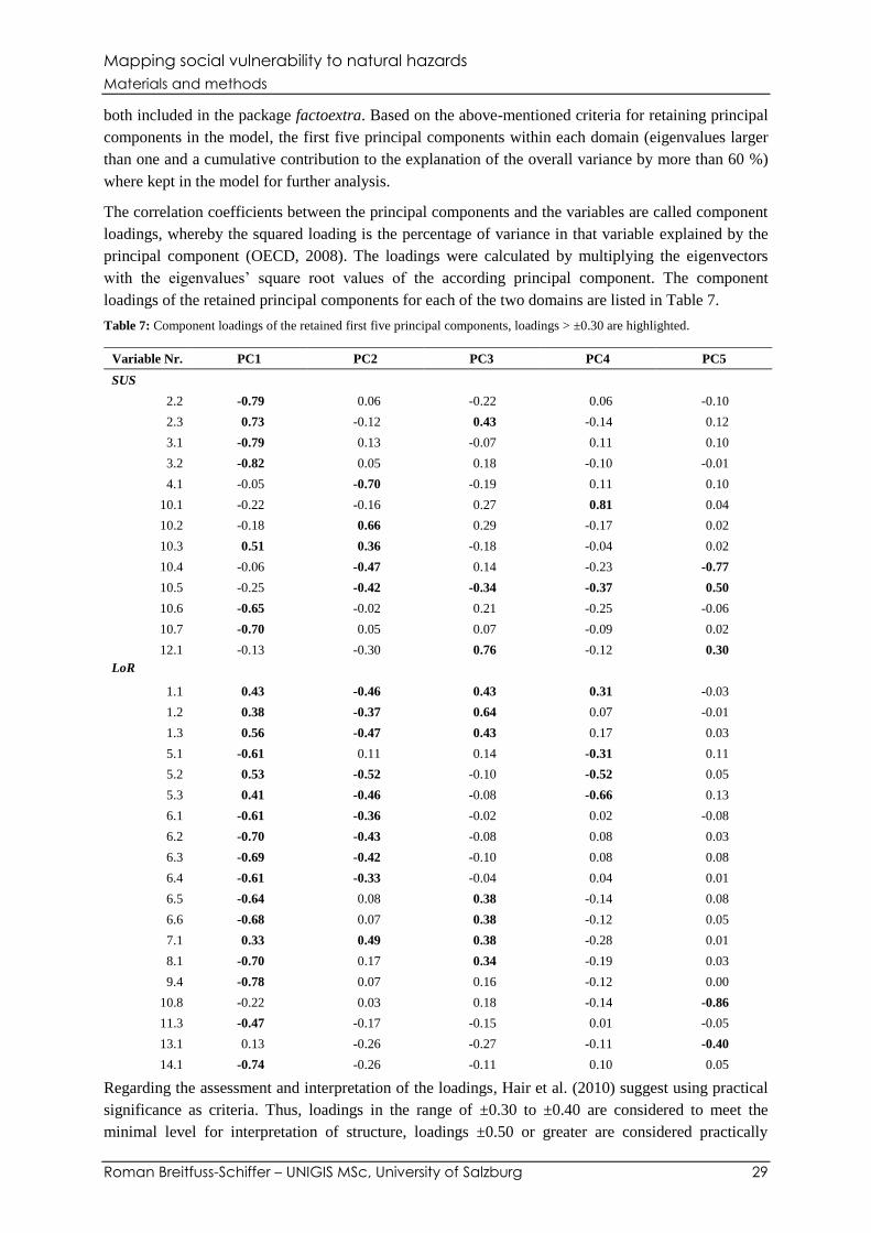
Mapping social vulnerability to natural hazards
Materials and methods
Roman Breitfuss-Schiffer – UNIGIS MSc, University of Salzburg 29
both included in the package factoextra. Based on the above-mentioned criteria for retaining principal
components in the model, the first five principal components within each domain (eigenvalues larger
than one and a cumulative contribution to the explanation of the overall variance by more than 60 %)
where kept in the model for further analysis.
The correlation coefficients between the principal components and the variables are called component
loadings, whereby the squared loading is the percentage of variance in that variable explained by the
principal component (OECD, 2008). The loadings were calculated by multiplying the eigenvectors
with the eigenvalues’ square root values of the according principal component. The component
loadings of the retained principal components for each of the two domains are listed in Table 7.
Table 7: Component loadings of the retained first five principal components, loadings > ±0.30 are highlighted.
Variable Nr. PC1 PC2 PC3 PC4 PC5
SUS
2.2 -0.79 0.06 -0.22 0.06 -0.10
2.3 0.73 -0.12 0.43 -0.14 0.12
3.1 -0.79 0.13 -0.07 0.11 0.10
3.2 -0.82 0.05 0.18 -0.10 -0.01
4.1 -0.05 -0.70 -0.19 0.11 0.10
10.1 -0.22 -0.16 0.27 0.81 0.04
10.2 -0.18 0.66 0.29 -0.17 0.02
10.3 0.51 0.36 -0.18 -0.04 0.02
10.4 -0.06 -0.47 0.14 -0.23 -0.77
10.5 -0.25 -0.42 -0.34 -0.37 0.50
10.6 -0.65 -0.02 0.21 -0.25 -0.06
10.7 -0.70 0.05 0.07 -0.09 0.02
12.1 -0.13 -0.30 0.76 -0.12 0.30
LoR
1.1 0.43 -0.46 0.43 0.31 -0.03
1.2 0.38 -0.37 0.64 0.07 -0.01
1.3 0.56 -0.47 0.43 0.17 0.03
5.1 -0.61 0.11 0.14 -0.31 0.11
5.2 0.53 -0.52 -0.10 -0.52 0.05
5.3 0.41 -0.46 -0.08 -0.66 0.13
6.1 -0.61 -0.36 -0.02 0.02 -0.08
6.2 -0.70 -0.43 -0.08 0.08 0.03
6.3 -0.69 -0.42 -0.10 0.08 0.08
6.4 -0.61 -0.33 -0.04 0.04 0.01
6.5 -0.64 0.08 0.38 -0.14 0.08
6.6 -0.68 0.07 0.38 -0.12 0.05
7.1 0.33 0.49 0.38 -0.28 0.01
8.1 -0.70 0.17 0.34 -0.19 0.03
9.4 -0.78 0.07 0.16 -0.12 0.00
10.8 -0.22 0.03 0.18 -0.14 -0.86
11.3 -0.47 -0.17 -0.15 0.01 -0.05
13.1 0.13 -0.26 -0.27 -0.11 -0.40
14.1 -0.74 -0.26 -0.11 0.10 0.05
Regarding the assessment and interpretation of the loadings, Hair et al. (2010) suggest using practical
significance as criteria. Thus, loadings in the range of ±0.30 to ±0.40 are considered to meet the
minimal level for interpretation of structure, loadings ±0.50 or greater are considered practically
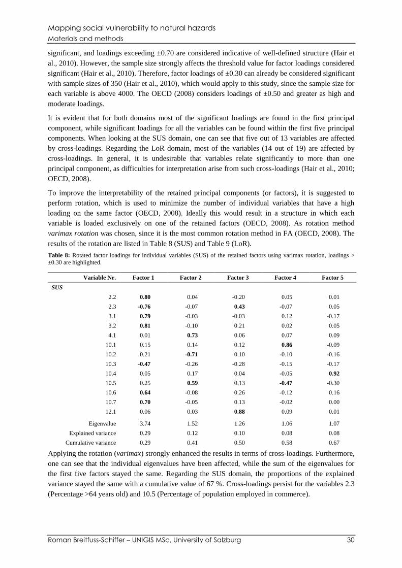
Mapping social vulnerability to natural hazards
Materials and methods
Roman Breitfuss-Schiffer – UNIGIS MSc, University of Salzburg 30
significant, and loadings exceeding ±0.70 are considered indicative of well-defined structure (Hair et
al., 2010). However, the sample size strongly affects the threshold value for factor loadings considered
significant (Hair et al., 2010). Therefore, factor loadings of ±0.30 can already be considered significant
with sample sizes of 350 (Hair et al., 2010), which would apply to this study, since the sample size for
each variable is above 4000. The OECD (2008) considers loadings of ±0.50 and greater as high and
moderate loadings.
It is evident that for both domains most of the significant loadings are found in the first principal
component, while significant loadings for all the variables can be found within the first five principal
components. When looking at the SUS domain, one can see that five out of 13 variables are affected
by cross-loadings. Regarding the LoR domain, most of the variables (14 out of 19) are affected by
cross-loadings. In general, it is undesirable that variables relate significantly to more than one
principal component, as difficulties for interpretation arise from such cross-loadings (Hair et al., 2010;
OECD, 2008).
To improve the interpretability of the retained principal components (or factors), it is suggested to
perform rotation, which is used to minimize the number of individual variables that have a high
loading on the same factor (OECD, 2008). Ideally this would result in a structure in which each
variable is loaded exclusively on one of the retained factors (OECD, 2008). As rotation method
varimax rotation was chosen, since it is the most common rotation method in FA (OECD, 2008). The
results of the rotation are listed in Table 8 (SUS) and Table 9 (LoR).
Table 8: Rotated factor loadings for individual variables (SUS) of the retained factors using varimax rotation, loadings >
±0.30 are highlighted.
Variable Nr. Factor 1 Factor 2 Factor 3 Factor 4 Factor 5
SUS
2.2 0.80 0.04 -0.20 0.05 0.01
2.3 -0.76 -0.07 0.43 -0.07 0.05
3.1 0.79 -0.03 -0.03 0.12 -0.17
3.2 0.81 -0.10 0.21 0.02 0.05
4.1 0.01 0.73 0.06 0.07 0.09
10.1 0.15 0.14 0.12 0.86 -0.09
10.2 0.21 -0.71 0.10 -0.10 -0.16
10.3 -0.47 -0.26 -0.28 -0.15 -0.17
10.4 0.05 0.17 0.04 -0.05 0.92
10.5 0.25 0.59 0.13 -0.47 -0.30
10.6 0.64 -0.08 0.26 -0.12 0.16
10.7 0.70 -0.05 0.13 -0.02 0.00
12.1 0.06 0.03 0.88 0.09 0.01
Eigenvalue 3.74 1.52 1.26 1.06 1.07
Explained variance 0.29 0.12 0.10 0.08 0.08
Cumulative variance 0.29 0.41 0.50 0.58 0.67
Applying the rotation (varimax) strongly enhanced the results in terms of cross-loadings. Furthermore,
one can see that the individual eigenvalues have been affected, while the sum of the eigenvalues for
the first five factors stayed the same. Regarding the SUS domain, the proportions of the explained
variance stayed the same with a cumulative value of 67 %. Cross-loadings persist for the variables 2.3
(Percentage >64 years old) and 10.5 (Percentage of population employed in commerce).
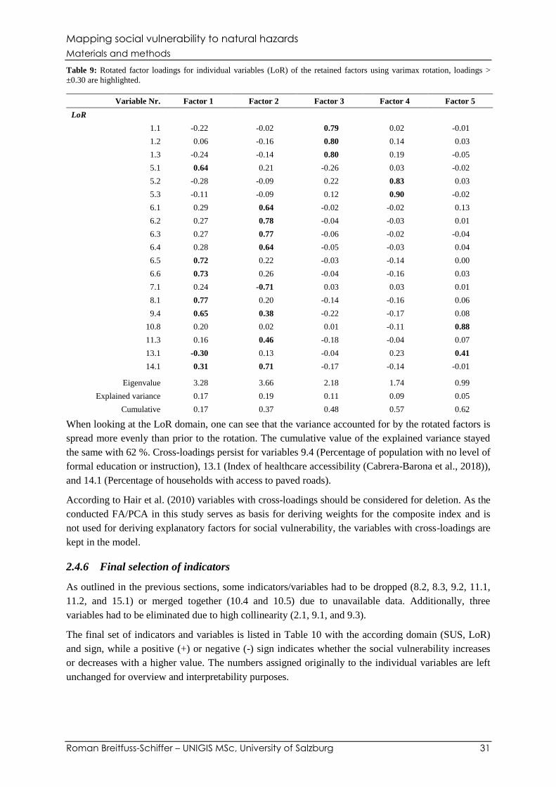
Mapping social vulnerability to natural hazards
Materials and methods
Roman Breitfuss-Schiffer – UNIGIS MSc, University of Salzburg 31
Table 9: Rotated factor loadings for individual variables (LoR) of the retained factors using varimax rotation, loadings >
±0.30 are highlighted.
Variable Nr. Factor 1 Factor 2 Factor 3 Factor 4 Factor 5
LoR
1.1 -0.22 -0.02 0.79 0.02 -0.01
1.2 0.06 -0.16 0.80 0.14 0.03
1.3 -0.24 -0.14 0.80 0.19 -0.05
5.1 0.64 0.21 -0.26 0.03 -0.02
5.2 -0.28 -0.09 0.22 0.83 0.03
5.3 -0.11 -0.09 0.12 0.90 -0.02
6.1 0.29 0.64 -0.02 -0.02 0.13
6.2 0.27 0.78 -0.04 -0.03 0.01
6.3 0.27 0.77 -0.06 -0.02 -0.04
6.4 0.28 0.64 -0.05 -0.03 0.04
6.5 0.72 0.22 -0.03 -0.14 0.00
6.6 0.73 0.26 -0.04 -0.16 0.03
7.1 0.24 -0.71 0.03 0.03 0.01
8.1 0.77 0.20 -0.14 -0.16 0.06
9.4 0.65 0.38 -0.22 -0.17 0.08
10.8 0.20 0.02 0.01 -0.11 0.88
11.3 0.16 0.46 -0.18 -0.04 0.07
13.1 -0.30 0.13 -0.04 0.23 0.41
14.1 0.31 0.71 -0.17 -0.14 -0.01
Eigenvalue 3.28 3.66 2.18 1.74 0.99
Explained variance 0.17 0.19 0.11 0.09 0.05
Cumulative 0.17 0.37 0.48 0.57 0.62
When looking at the LoR domain, one can see that the variance accounted for by the rotated factors is
spread more evenly than prior to the rotation. The cumulative value of the explained variance stayed
the same with 62 %. Cross-loadings persist for variables 9.4 (Percentage of population with no level of
formal education or instruction), 13.1 (Index of healthcare accessibility (Cabrera-Barona et al., 2018)),
and 14.1 (Percentage of households with access to paved roads).
According to Hair et al. (2010) variables with cross-loadings should be considered for deletion. As the
conducted FA/PCA in this study serves as basis for deriving weights for the composite index and is
not used for deriving explanatory factors for social vulnerability, the variables with cross-loadings are
kept in the model.
2.4.6 Final selection of indicators
As outlined in the previous sections, some indicators/variables had to be dropped (8.2, 8.3, 9.2, 11.1,
11.2, and 15.1) or merged together (10.4 and 10.5) due to unavailable data. Additionally, three
variables had to be eliminated due to high collinearity (2.1, 9.1, and 9.3).
The final set of indicators and variables is listed in Table 10 with the according domain (SUS, LoR)
and sign, while a positive (+) or negative (-) sign indicates whether the social vulnerability increases
or decreases with a higher value. The numbers assigned originally to the individual variables are left
unchanged for overview and interpretability purposes.
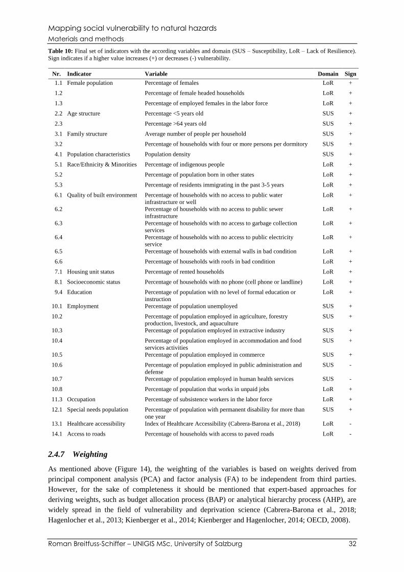
Mapping social vulnerability to natural hazards
Materials and methods
Roman Breitfuss-Schiffer – UNIGIS MSc, University of Salzburg 32
Table 10: Final set of indicators with the according variables and domain (SUS – Susceptibility, LoR – Lack of Resilience).
Sign indicates if a higher value increases (+) or decreases (-) vulnerability.
Nr. Indicator Variable Domain Sign
1.1 Female population Percentage of females LoR +
1.2 Percentage of female headed households LoR +
1.3 Percentage of employed females in the labor force LoR +
2.2 Age structure Percentage <5 years old SUS +
2.3 Percentage >64 years old SUS +
3.1 Family structure Average number of people per household SUS +
3.2 Percentage of households with four or more persons per dormitory SUS +
4.1 Population characteristics Population density SUS +
5.1 Race/Ethnicity & Minorities Percentage of indigenous people LoR +
5.2 Percentage of population born in other states LoR +
5.3 Percentage of residents immigrating in the past 3-5 years LoR +
6.1 Quality of built environment Percentage of households with no access to public water
infrastructure or well
LoR +
6.2 Percentage of households with no access to public sewer
infrastructure
LoR +
6.3 Percentage of households with no access to garbage collection
services
LoR +
6.4 Percentage of households with no access to public electricity
service
LoR +
6.5 Percentage of households with external walls in bad condition LoR +
6.6 Percentage of households with roofs in bad condition LoR +
7.1 Housing unit status Percentage of rented households LoR +
8.1 Socioeconomic status Percentage of households with no phone (cell phone or landline) LoR +
9.4 Education Percentage of population with no level of formal education or
instruction
LoR +
10.1 Employment Percentage of population unemployed SUS +
10.2 Percentage of population employed in agriculture, forestry
production, livestock, and aquaculture
SUS +
10.3 Percentage of population employed in extractive industry SUS +
10.4 Percentage of population employed in accommodation and food
services activities
SUS +
10.5 Percentage of population employed in commerce SUS +
10.6 Percentage of population employed in public administration and
defense
SUS -
10.7 Percentage of population employed in human health services SUS -
10.8 Percentage of population that works in unpaid jobs LoR +
11.3 Occupation Percentage of subsistence workers in the labor force LoR +
12.1 Special needs population Percentage of population with permanent disability for more than
one year
SUS +
13.1 Healthcare accessibility Index of Healthcare Accessibility (Cabrera-Barona et al., 2018) LoR -
14.1 Access to roads Percentage of households with access to paved roads LoR -
2.4.7 Weighting
As mentioned above (Figure 14), the weighting of the variables is based on weights derived from
principal component analysis (PCA) and factor analysis (FA) to be independent from third parties.
However, for the sake of completeness it should be mentioned that expert-based approaches for
deriving weights, such as budget allocation process (BAP) or analytical hierarchy process (AHP), are
widely spread in the field of vulnerability and deprivation science (Cabrera-Barona et al., 2018;
Hagenlocher et al., 2013; Kienberger et al., 2014; Kienberger and Hagenlocher, 2014; OECD, 2008).
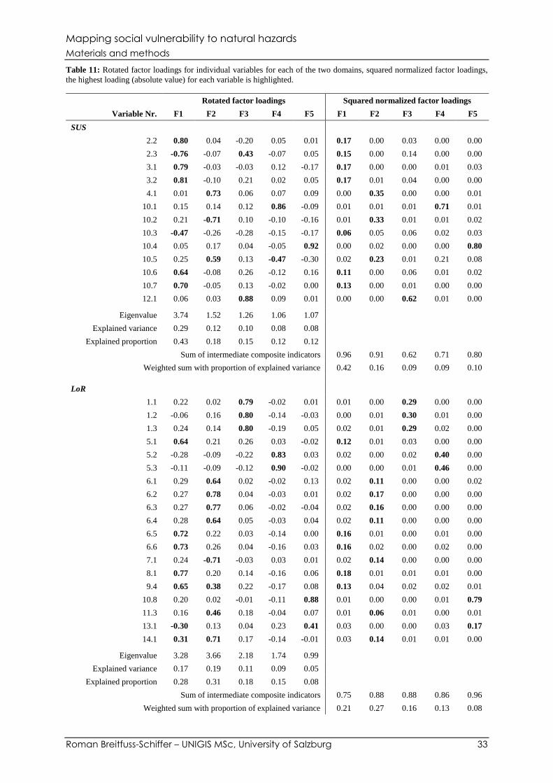
Mapping social vulnerability to natural hazards
Materials and methods
Roman Breitfuss-Schiffer – UNIGIS MSc, University of Salzburg 33
Table 11: Rotated factor loadings for individual variables for each of the two domains, squared normalized factor loadings,
the highest loading (absolute value) for each variable is highlighted.
Rotated factor loadings Squared normalized factor loadings
Variable Nr. F1 F2 F3 F4 F5 F1 F2 F3 F4 F5
SUS
2.2 0.80 0.04 -0.20 0.05 0.01 0.17 0.00 0.03 0.00 0.00
2.3 -0.76 -0.07 0.43 -0.07 0.05 0.15 0.00 0.14 0.00 0.00
3.1 0.79 -0.03 -0.03 0.12 -0.17 0.17 0.00 0.00 0.01 0.03
3.2 0.81 -0.10 0.21 0.02 0.05 0.17 0.01 0.04 0.00 0.00
4.1 0.01 0.73 0.06 0.07 0.09 0.00 0.35 0.00 0.00 0.01
10.1 0.15 0.14 0.12 0.86 -0.09 0.01 0.01 0.01 0.71 0.01
10.2 0.21 -0.71 0.10 -0.10 -0.16 0.01 0.33 0.01 0.01 0.02
10.3 -0.47 -0.26 -0.28 -0.15 -0.17 0.06 0.05 0.06 0.02 0.03
10.4 0.05 0.17 0.04 -0.05 0.92 0.00 0.02 0.00 0.00 0.80
10.5 0.25 0.59 0.13 -0.47 -0.30 0.02 0.23 0.01 0.21 0.08
10.6 0.64 -0.08 0.26 -0.12 0.16 0.11 0.00 0.06 0.01 0.02
10.7 0.70 -0.05 0.13 -0.02 0.00 0.13 0.00 0.01 0.00 0.00
12.1 0.06 0.03 0.88 0.09 0.01 0.00 0.00 0.62 0.01 0.00
Eigenvalue 3.74 1.52 1.26 1.06 1.07
Explained variance 0.29 0.12 0.10 0.08 0.08
Explained proportion 0.43 0.18 0.15 0.12 0.12
Sum of intermediate composite indicators 0.96 0.91 0.62 0.71 0.80
Weighted sum with proportion of explained variance 0.42 0.16 0.09 0.09 0.10
LoR
1.1 0.22 0.02 0.79 -0.02 0.01 0.01 0.00 0.29 0.00 0.00
1.2 -0.06 0.16 0.80 -0.14 -0.03 0.00 0.01 0.30 0.01 0.00
1.3 0.24 0.14 0.80 -0.19 0.05 0.02 0.01 0.29 0.02 0.00
5.1 0.64 0.21 0.26 0.03 -0.02 0.12 0.01 0.03 0.00 0.00
5.2 -0.28 -0.09 -0.22 0.83 0.03 0.02 0.00 0.02 0.40 0.00
5.3 -0.11 -0.09 -0.12 0.90 -0.02 0.00 0.00 0.01 0.46 0.00
6.1 0.29 0.64 0.02 -0.02 0.13 0.02 0.11 0.00 0.00 0.02
6.2 0.27 0.78 0.04 -0.03 0.01 0.02 0.17 0.00 0.00 0.00
6.3 0.27 0.77 0.06 -0.02 -0.04 0.02 0.16 0.00 0.00 0.00
6.4 0.28 0.64 0.05 -0.03 0.04 0.02 0.11 0.00 0.00 0.00
6.5 0.72 0.22 0.03 -0.14 0.00 0.16 0.01 0.00 0.01 0.00
6.6 0.73 0.26 0.04 -0.16 0.03 0.16 0.02 0.00 0.02 0.00
7.1 0.24 -0.71 -0.03 0.03 0.01 0.02 0.14 0.00 0.00 0.00
8.1 0.77 0.20 0.14 -0.16 0.06 0.18 0.01 0.01 0.01 0.00
9.4 0.65 0.38 0.22 -0.17 0.08 0.13 0.04 0.02 0.02 0.01
10.8 0.20 0.02 -0.01 -0.11 0.88 0.01 0.00 0.00 0.01 0.79
11.3 0.16 0.46 0.18 -0.04 0.07 0.01 0.06 0.01 0.00 0.01
13.1 -0.30 0.13 0.04 0.23 0.41 0.03 0.00 0.00 0.03 0.17
14.1 0.31 0.71 0.17 -0.14 -0.01 0.03 0.14 0.01 0.01 0.00
Eigenvalue 3.28 3.66 2.18 1.74 0.99
Explained variance 0.17 0.19 0.11 0.09 0.05
Explained proportion 0.28 0.31 0.18 0.15 0.08
Sum of intermediate composite indicators 0.75 0.88 0.88 0.86 0.96
Weighted sum with proportion of explained variance 0.21 0.27 0.16 0.13 0.08

Mapping social vulnerability to natural hazards
Materials and methods
Roman Breitfuss-Schiffer – UNIGIS MSc, University of Salzburg 34
The variable weightings are calculated for each of the two domains separately and are derived from
results of the factor analysis. The weights for the individual variables are constructed based on the
factor loadings after rotation, whereby the squared factor loadings represent the proportion of the total
unit variance of the variable which is explained by the factor (Nicoletti et al., 2000; OECD, 2008). The
highest squared and normalized factor loadings for each individual variable are grouped into
intermediate composite indicators each representing one factor (Nicoletti et al., 2000; OECD, 2008).
Table 12: Indicators with the according variables, signs, and weights grouped by domain (SUS, LoR).
Nr. Indicator Variable Sign Weight
SUS
2.2 Age structure Percentage <5 years old + 0.09
2.3 Percentage >64 years old + 0.08
3.1 Family structure Average number of people per household + 0.08
3.2 Percentage of households with four or more persons per dormitory + 0.09
4.1 Population characteristics Population density + 0.07
10.1 Employment Percentage of population unemployed + 0.10
10.2 Percentage of population employed in agriculture, forestry
production, livestock, and aquaculture
+ 0.07
10.3 Percentage of population employed in extractive industry + 0.03
10.4 Percentage of population employed in accommodation and food
services activities
+ 0.11
10.5 Percentage of population employed in commerce + 0.05
10.6 Percentage of population employed in public administration and
defense
- 0.06
10.7 Percentage of population employed in human health services - 0.07
12.1 Special needs population Percentage of population with permanent disability for more than
one year
+ 0.10
LoR
1.1 Female population Percentage of females - 0.06
1.2 Percentage of female headed households - 0.07
1.3 Percentage of employed females in the labor force - 0.06
5.1 Race/Ethnicity & Minorities Percentage of indigenous people + 0.04
5.2 Percentage of population born in other states + 0.07
5.3 Percentage of residents immigrating in the past 3-5 years + 0.08
6.1 Quality of built environment Percentage of households with no access to public water
infrastructure or well
+ 0.04
6.2 Percentage of households with no access to public sewer
infrastructure
+ 0.06
6.3 Percentage of households with no access to garbage collection
services
+ 0.06
6.4 Percentage of households with no access to public electricity
service
+ 0.04
6.5 Percentage of households with external walls in bad condition + 0.05
6.6 Percentage of households with roofs in bad condition + 0.05
7.1 Housing unit status Percentage of rented households + 0.05
8.1 Socioeconomic status Percentage of households with no phone (cell phone or landline) + 0.06
9.4 Education Percentage of population with no level of formal education or
instruction
+ 0.04
10.8 Employment Percentage of population that works in unpaid jobs + 0.08
11.3 Occupation Percentage of subsistence workers in the labor force + 0.02
13.1 Healthcare accessibility Index of Healthcare Accessibility (Cabrera-Barona et al., 2018) - 0.02
14.1 Access to roads Percentage of households with access to paved roads - 0.05
Mapping social vulnerability to natural hazards
Materials and methods
Roman Breitfuss-Schiffer – UNIGIS MSc, University of Salzburg 35
Table 11 shows the rotated factor loadings and the squared normalized factor loadings for each of the
two domains, while the highest loading for each variable is highlighted. Furthermore, the proportion of
explained variance of each factor and the weighted sum of the intermediate composite indicators are
listed. For deriving the weights for each individual variable, the corresponding highest factor loading
is weighted according to the proportion of the explained variance of the factor in which the highest
loading occurs and then normalized by the sum of weighted intermediate composite indicators
(OECD, 2008).
Table 12 shows the indicators/variables grouped by domain with their according sign and derived
weight. Note that the weights within each of the two domains sum up to one.
2.4.8 Aggregation
The normalized variables were aggregated within each of the two domains following equation 3
(Hagenlocher et al., 2013; OECD, 2008). While this aggregation method is widely spread, one has to
keep in mind that the composite indicator depends on the quality of the underlying individual variables
and that a condition for additive aggregation is that the individual variables are mutually independent
(OECD, 2008). Hence, additive aggregation allows the assessment of the marginal contribution of
each variable separately, which might be a rather unrealistic assumption for many phenomena (OECD,
2008). Therefore, the aggregation could result in a biased composite indicator, whereby the dimension
and the direction of the error are not easily determined and an adjustment of the composite indicator
cannot be carried out properly (OECD, 2008). Nevertheless, linear aggregation is by far the most
widespread aggregation method (OECD, 2008), especially in the domain of vulnerability studies (e.g.
Chen et al., 2014; de Loyola Hummell et al., 2016; Fatemi et al., 2017; Hagenlocher et al., 2013;
Kienberger et al., 2014; Yoon, 2012), and therefore is chosen as aggregation method for this study.
The aggregation of the two domains (SUS, LoR) to the composite indicator of social vulnerability was
calculated following equation 4 taking into account specific weights for each of the two domains
(Hagenlocher et al., 2013). The weights were derived from the number of variables in each domain in
relation to the total number of variables resulting in a weight of 0.41 and 0.59 in the SUS domain (13
variables divided by 32 total variables) and in the LoR domain (19 variables divided by 32 total
variables), respectively.
𝑆𝑈𝑆/𝐿𝑜𝑅 =∑𝑤𝑖𝑣𝑖′
𝑛
𝑖=1
(3)
𝑆𝑈𝑆/𝐿𝑜𝑅 vulnerability domain
𝑤𝑖 weight of variable i
𝑣𝑖’ normalized value (min-max) of variable i
𝑉𝑈 =∑𝑤𝑗𝑋𝑗
𝑛
𝑗=1
(4)
𝑉𝑈 composite index for social vulnerability
𝑤𝑗 weight of domain j
𝑋𝑗 normalized value (min-max) of domain j
To enhance and facilitate interpretation of the final composite index for social vulnerability, the index
was scaled between 0.0 and 1.0 (min-max normalization), where 0.0 indicating a very low social
vulnerability and 1.0 indicating a very high social vulnerability (Cabrera-Barona et al., 2018;
Hagenlocher et al., 2013).
Mapping social vulnerability to natural hazards
Materials and methods
Roman Breitfuss-Schiffer – UNIGIS MSc, University of Salzburg 36
2.4.9 Hot and cold spot analysis
Hot and cold spot analysis was conducted on the composite index for social vulnerability to assess the
degree of spatial correlation throughout the study area (Mazumdar and Paul, 2018). Getis-Ord Gi*
statistics were applied to display the spatial pattern in social vulnerability (Ord and Getis, 1995).
Statistically significant z-scores are used for locating and making visible hot and cold spots (clustering
of high and low values) for 99, 95 and 90 % confidence level (Anselin, 1995; Ord and Getis, 1995).
The analysis was carried out with ArcGIS Pro (Tool Hot-Spot Analysis (Getis-Ord Gi*)), while the
fixed distance band option was used to conceptualize spatial relationships to ensure that each polygon
will have at least one neighbor taken into account for the spatial analysis. A threshold distance of
590.4 m was calculated by applying the tool Distance Band from Neighborhood Count. Furthermore,
false discovery rate (FDR) correction was applied, as it yields better results identifying local spatial
clusters (Castro and Singer, 2006).
2.4.10 Visualization and mapping
The visualization and mapping of the composite index, the individual variables as well as the results of
the hot and cold spot analysis were realized with the Software ArcGIS Pro. The figures are integrated
in section 3 (Results).

Mapping social vulnerability to natural hazards
Results
Roman Breitfuss-Schiffer – UNIGIS MSc, University of Salzburg 37
3. Results
3.1 Vulnerability variables
After treating outliers and conducting multivariate statistical analysis (i.e. test for multicollinearities
and PCA/FA), a total of 32 social vulnerability variables representing two vulnerability domains
(SUS, LoR) were retained for the construction of the composite index. Overviews of the final set of
variables with the according domains, signs and weights are provided in Table 10 and Table 12 (see
2.4.6 and 2.4.7). The visualization (Figure 18 and Figure 19) of the spatial distribution of the
individual variables (min-max normalized values) gives a first impression of the city of Quito’s socio-
economic characteristics.
Figure 18: Spatial distribution of the final selection of susceptibility (SUS) variables (min-max normalized values) within the
study area with the assigned weight.
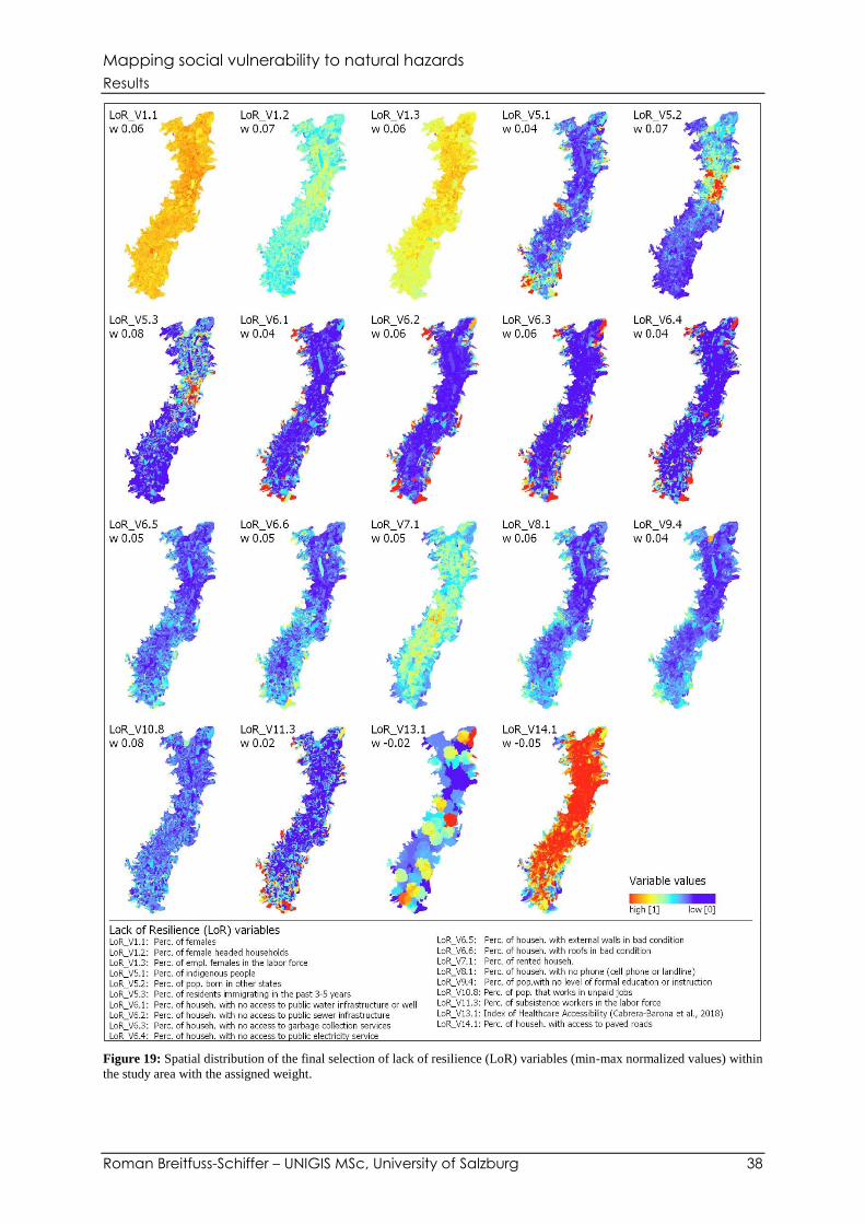
Mapping social vulnerability to natural hazards
Results
Roman Breitfuss-Schiffer – UNIGIS MSc, University of Salzburg 38
Figure 19: Spatial distribution of the final selection of lack of resilience (LoR) variables (min-max normalized values) within
the study area with the assigned weight.
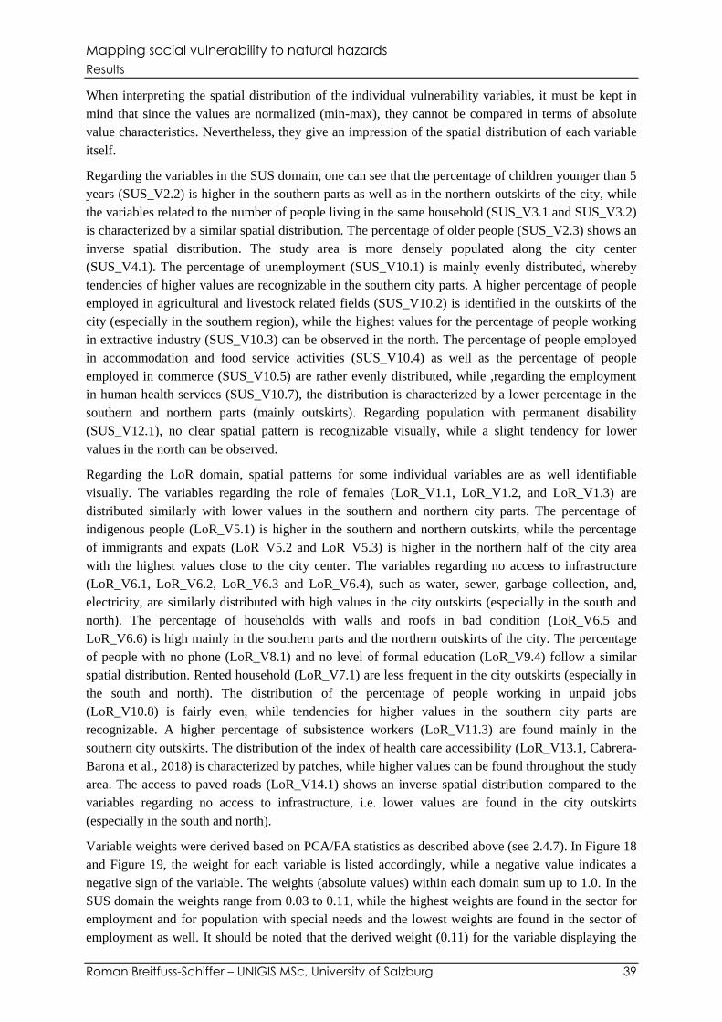
Mapping social vulnerability to natural hazards
Results
Roman Breitfuss-Schiffer – UNIGIS MSc, University of Salzburg 39
When interpreting the spatial distribution of the individual vulnerability variables, it must be kept in
mind that since the values are normalized (min-max), they cannot be compared in terms of absolute
value characteristics. Nevertheless, they give an impression of the spatial distribution of each variable
itself.
Regarding the variables in the SUS domain, one can see that the percentage of children younger than 5
years (SUS_V2.2) is higher in the southern parts as well as in the northern outskirts of the city, while
the variables related to the number of people living in the same household (SUS_V3.1 and SUS_V3.2)
is characterized by a similar spatial distribution. The percentage of older people (SUS_V2.3) shows an
inverse spatial distribution. The study area is more densely populated along the city center
(SUS_V4.1). The percentage of unemployment (SUS_V10.1) is mainly evenly distributed, whereby
tendencies of higher values are recognizable in the southern city parts. A higher percentage of people
employed in agricultural and livestock related fields (SUS_V10.2) is identified in the outskirts of the
city (especially in the southern region), while the highest values for the percentage of people working
in extractive industry (SUS_V10.3) can be observed in the north. The percentage of people employed
in accommodation and food service activities (SUS_V10.4) as well as the percentage of people
employed in commerce (SUS_V10.5) are rather evenly distributed, while ,regarding the employment
in human health services (SUS_V10.7), the distribution is characterized by a lower percentage in the
southern and northern parts (mainly outskirts). Regarding population with permanent disability
(SUS_V12.1), no clear spatial pattern is recognizable visually, while a slight tendency for lower
values in the north can be observed.
Regarding the LoR domain, spatial patterns for some individual variables are as well identifiable
visually. The variables regarding the role of females (LoR_V1.1, LoR_V1.2, and LoR_V1.3) are
distributed similarly with lower values in the southern and northern city parts. The percentage of
indigenous people (LoR_V5.1) is higher in the southern and northern outskirts, while the percentage
of immigrants and expats (LoR_V5.2 and LoR_V5.3) is higher in the northern half of the city area
with the highest values close to the city center. The variables regarding no access to infrastructure
(LoR_V6.1, LoR_V6.2, LoR_V6.3 and LoR_V6.4), such as water, sewer, garbage collection, and,
electricity, are similarly distributed with high values in the city outskirts (especially in the south and
north). The percentage of households with walls and roofs in bad condition (LoR_V6.5 and
LoR_V6.6) is high mainly in the southern parts and the northern outskirts of the city. The percentage
of people with no phone (LoR_V8.1) and no level of formal education (LoR_V9.4) follow a similar
spatial distribution. Rented household (LoR_V7.1) are less frequent in the city outskirts (especially in
the south and north). The distribution of the percentage of people working in unpaid jobs
(LoR_V10.8) is fairly even, while tendencies for higher values in the southern city parts are
recognizable. A higher percentage of subsistence workers (LoR_V11.3) are found mainly in the
southern city outskirts. The distribution of the index of health care accessibility (LoR_V13.1, Cabrera-
Barona et al., 2018) is characterized by patches, while higher values can be found throughout the study
area. The access to paved roads (LoR_V14.1) shows an inverse spatial distribution compared to the
variables regarding no access to infrastructure, i.e. lower values are found in the city outskirts
(especially in the south and north).
Variable weights were derived based on PCA/FA statistics as described above (see 2.4.7). In Figure 18
and Figure 19, the weight for each variable is listed accordingly, while a negative value indicates a
negative sign of the variable. The weights (absolute values) within each domain sum up to 1.0. In the
SUS domain the weights range from 0.03 to 0.11, while the highest weights are found in the sector for
employment and for population with special needs and the lowest weights are found in the sector of
employment as well. It should be noted that the derived weight (0.11) for the variable displaying the
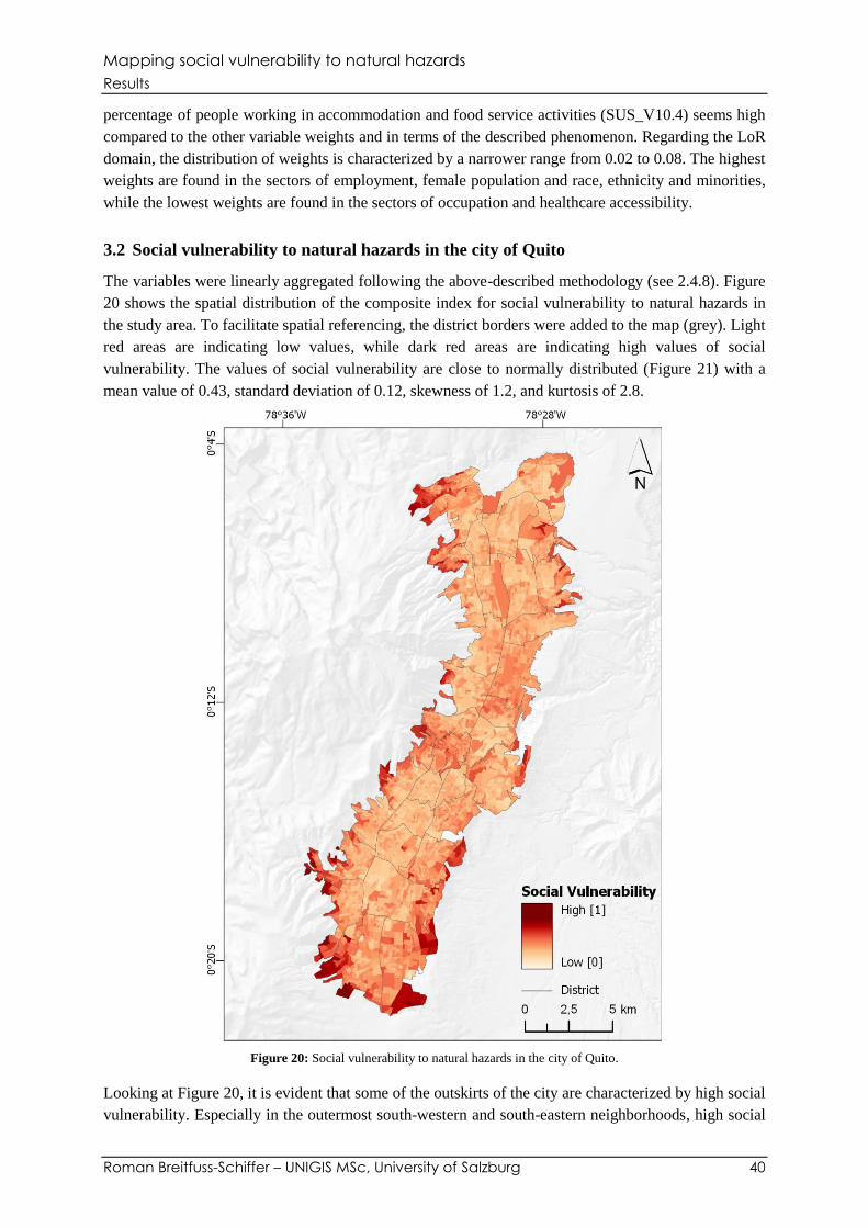
Mapping social vulnerability to natural hazards
Results
Roman Breitfuss-Schiffer – UNIGIS MSc, University of Salzburg 40
percentage of people working in accommodation and food service activities (SUS_V10.4) seems high
compared to the other variable weights and in terms of the described phenomenon. Regarding the LoR
domain, the distribution of weights is characterized by a narrower range from 0.02 to 0.08. The highest
weights are found in the sectors of employment, female population and race, ethnicity and minorities,
while the lowest weights are found in the sectors of occupation and healthcare accessibility.
3.2 Social vulnerability to natural hazards in the city of Quito
The variables were linearly aggregated following the above-described methodology (see 2.4.8). Figure
20 shows the spatial distribution of the composite index for social vulnerability to natural hazards in
the study area. To facilitate spatial referencing, the district borders were added to the map (grey). Light
red areas are indicating low values, while dark red areas are indicating high values of social
vulnerability. The values of social vulnerability are close to normally distributed (Figure 21) with a
mean value of 0.43, standard deviation of 0.12, skewness of 1.2, and kurtosis of 2.8.
Figure 20: Social vulnerability to natural hazards in the city of Quito.
Looking at Figure 20, it is evident that some of the outskirts of the city are characterized by high social
vulnerability. Especially in the outermost south-western and south-eastern neighborhoods, high social
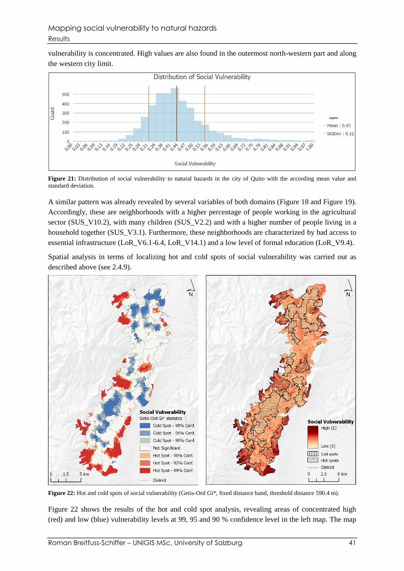
Mapping social vulnerability to natural hazards
Results
Roman Breitfuss-Schiffer – UNIGIS MSc, University of Salzburg 41
vulnerability is concentrated. High values are also found in the outermost north-western part and along
the western city limit.
Figure 21: Distribution of social vulnerability to natural hazards in the city of Quito with the according mean value and
standard deviation.
A similar pattern was already revealed by several variables of both domains (Figure 18 and Figure 19).
Accordingly, these are neighborhoods with a higher percentage of people working in the agricultural
sector (SUS_V10.2), with many children (SUS_V2.2) and with a higher number of people living in a
household together (SUS_V3.1). Furthermore, these neighborhoods are characterized by bad access to
essential infrastructure (LoR_V6.1-6.4, LoR_V14.1) and a low level of formal education (LoR_V9.4).
Spatial analysis in terms of localizing hot and cold spots of social vulnerability was carried out as
described above (see 2.4.9).
Figure 22: Hot and cold spots of social vulnerability (Getis-Ord Gi*, fixed distance band, threshold distance 590.4 m).
Figure 22 shows the results of the hot and cold spot analysis, revealing areas of concentrated high
(red) and low (blue) vulnerability levels at 99, 95 and 90 % confidence level in the left map. The map
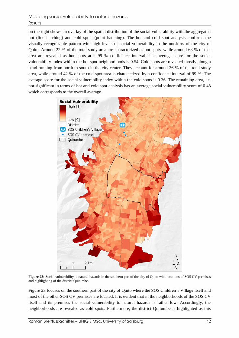
Mapping social vulnerability to natural hazards
Results
Roman Breitfuss-Schiffer – UNIGIS MSc, University of Salzburg 42
on the right shows an overlay of the spatial distribution of the social vulnerability with the aggregated
hot (line hatching) and cold spots (point hatching). The hot and cold spot analysis confirms the
visually recognizable pattern with high levels of social vulnerability in the outskirts of the city of
Quito. Around 22 % of the total study area are characterized as hot spots, while around 68 % of that
area are revealed as hot spots at a 99 % confidence interval. The average score for the social
vulnerability index within the hot spot neighborhoods is 0.54. Cold spots are revealed mostly along a
band running from north to south in the city center. They account for around 26 % of the total study
area, while around 42 % of the cold spot area is characterized by a confidence interval of 99 %. The
average score for the social vulnerability index within the cold spots is 0.36. The remaining area, i.e.
not significant in terms of hot and cold spot analysis has an average social vulnerability score of 0.43
which corresponds to the overall average.
Figure 23: Social vulnerability to natural hazards in the southern part of the city of Quito with locations of SOS CV premises
and highlighting of the district Quitumbe.
Figure 23 focuses on the southern part of the city of Quito where the SOS Children’s Village itself and
most of the other SOS CV premises are located. It is evident that in the neighborhoods of the SOS CV
itself and its premises the social vulnerability to natural hazards is rather low. Accordingly, the
neighborhoods are revealed as cold spots. Furthermore, the district Quitumbe is highlighted as this
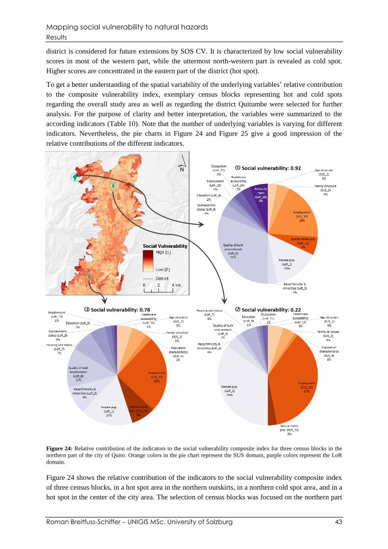
Mapping social vulnerability to natural hazards
Results
Roman Breitfuss-Schiffer – UNIGIS MSc, University of Salzburg 43
district is considered for future extensions by SOS CV. It is characterized by low social vulnerability
scores in most of the western part, while the uttermost north-western part is revealed as cold spot.
Higher scores are concentrated in the eastern part of the district (hot spot).
To get a better understanding of the spatial variability of the underlying variables’ relative contribution
to the composite vulnerability index, exemplary census blocks representing hot and cold spots
regarding the overall study area as well as regarding the district Quitumbe were selected for further
analysis. For the purpose of clarity and better interpretation, the variables were summarized to the
according indicators (Table 10). Note that the number of underlying variables is varying for different
indicators. Nevertheless, the pie charts in Figure 24 and Figure 25 give a good impression of the
relative contributions of the different indicators.
Figure 24: Relative contribution of the indicators to the social vulnerability composite index for three census blocks in the
northern part of the city of Quito. Orange colors in the pie chart represent the SUS domain, purple colors represent the LoR
domain.
Figure 24 shows the relative contribution of the indicators to the social vulnerability composite index
of three census blocks, in a hot spot area in the northern outskirts, in a northern cold spot area, and in a
hot spot in the center of the city area. The selection of census blocks was focused on the northern part
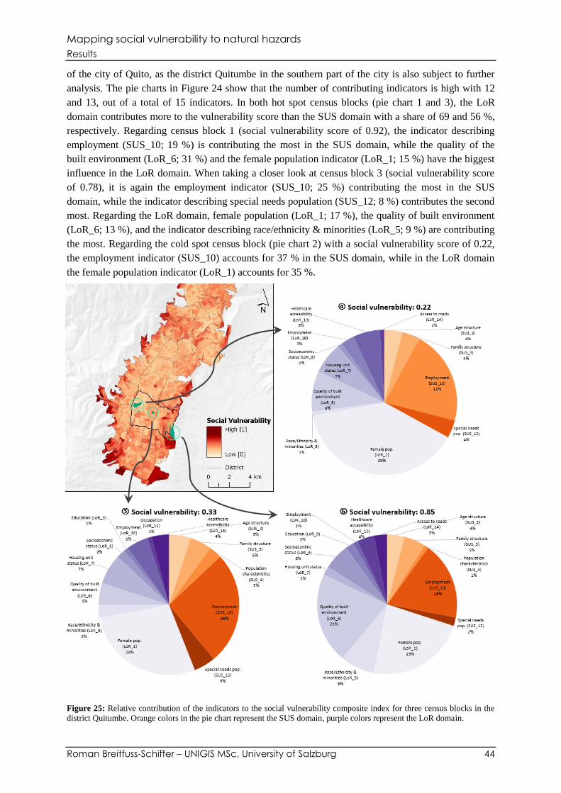
Mapping social vulnerability to natural hazards
Results
Roman Breitfuss-Schiffer – UNIGIS MSc, University of Salzburg 44
of the city of Quito, as the district Quitumbe in the southern part of the city is also subject to further
analysis. The pie charts in Figure 24 show that the number of contributing indicators is high with 12
and 13, out of a total of 15 indicators. In both hot spot census blocks (pie chart 1 and 3), the LoR
domain contributes more to the vulnerability score than the SUS domain with a share of 69 and 56 %,
respectively. Regarding census block 1 (social vulnerability score of 0.92), the indicator describing
employment (SUS_10; 19 %) is contributing the most in the SUS domain, while the quality of the
built environment (LoR_6; 31 %) and the female population indicator (LoR_1; 15 %) have the biggest
influence in the LoR domain. When taking a closer look at census block 3 (social vulnerability score
of 0.78), it is again the employment indicator (SUS_10; 25 %) contributing the most in the SUS
domain, while the indicator describing special needs population (SUS_12; 8 %) contributes the second
most. Regarding the LoR domain, female population (LoR_1; 17 %), the quality of built environment
(LoR_6; 13 %), and the indicator describing race/ethnicity & minorities (LoR_5; 9 %) are contributing
the most. Regarding the cold spot census block (pie chart 2) with a social vulnerability score of 0.22,
the employment indicator (SUS_10) accounts for 37 % in the SUS domain, while in the LoR domain
the female population indicator (LoR_1) accounts for 35 %.
Figure 25: Relative contribution of the indicators to the social vulnerability composite index for three census blocks in the
district Quitumbe. Orange colors in the pie chart represent the SUS domain, purple colors represent the LoR domain.

Mapping social vulnerability to natural hazards
Results
Roman Breitfuss-Schiffer – UNIGIS MSc, University of Salzburg 45
Figure 25 shows the relative contribution of the indicators to the social vulnerability composite index
of three census blocks in the district Quitumbe. They are located in a cold spot area in the western part
of district, in neither a cold nor hot spot area in the center of the district, and in a hot spot area in the
eastern part of the district. The pie charts in Figure 25 show that the number of contributing indicators
to the composite index of social vulnerability is also high in Quitumbe with 12 and 14, out of a total of
15 indicators. In all three census blocks (pie chart 4 to 6), the LoR domain contributes more to the
vulnerability score than the SUS domain with a share of 67, 56 and 70 %, respectively. Regarding
census block 4 in the cold spot area (social vulnerability score of 0.22), the employment indicator
(SUS_10; 21 %) contributes the most in the SUS domain, while the indicator describing female
population (LoR; 39 %) and the quality of built environment (LoR_6; 9 %) contribute the most in the
LoR domain. A similar pattern can be recognized regarding the census block 5 with a social
vulnerability score of 0.33. The employment indicator (SUS_10; 26 %) and the female population
indicator (LoR_1; 28 %) contribute the most in the SUS and in the LoR domain, respectively.
Regarding census block 6 in the hot spot area (social vulnerability score of 0.85), again, the
employment indicator (SUS_10; 18 %) contributes the most in the SUS domain, while the indicator
describing female population (LoR_1; 23 %), the quality of built environment (LoR_6; 21 %), and the
indicator describing race/ethnicity & minorities (LoR_5; 8 %) contribute the most in the LoR domain.
In general, the indicators describing employment (SUS_10), female population (LoR_1), and quality
of built environment (LoR_6 – access to public infrastructure, building condition of housing) account
for the largest shares of contribution throughout all six exemplary census blocks. However, the
contribution of the quality of built environment is higher in the outskirts (pie chart 1 and 6), while the
indicator plays a minor role regarding the more central areas (pie chart 2, 4, and 5), where the overall
social vulnerability score is lower. Also, the contribution of the female population indicator tends to be
higher in the more central areas (pie chart 2, 4, and 5), where the overall social vulnerability score is
lower. The employment indicator plays a major role in all six exemplary census blocks, while the
contribution also tends to be higher in the areas located more central (pie chart 2, 3, 4, and 5).
Despite the assessment of exposure to natural hazards is not part of this thesis, Figure 26 gives an
impression of the spatial distribution of natural hazards in the city of Quito such as mass movements,
floods, volcanic hazards and forest fires. The danger of mass movements is low from north to south in
the city center and tends to be higher along the city borders. The red dots represent different subtypes
of hazardous events (landslides, sinking, mudflows and rock falls) recorded from 2006 to 2017, while
landslides have the highest frequency. It is evident that the majority of the mass movement events
were recorded in the southern half of the city. Flood prone areas (high and low danger) are located
mostly along the minor rivers in the city area, while there is no river in close proximity to a larger
flood prone area in the northern half of the city. The higher danger in this area probably results from a
high degree of soil sealing and/or insufficient rainwater collecting systems (Municipio del Distrito
Metropolitano de Quito, 2015). The red dots represent flood events recorded from 2005 to 2017. One
can recognize a higher frequency of events along the areas prone to flood in the city center. Volcanic
hazards pose low to high danger along the western city border and minor danger in the northern and
southern uttermost outskirts. Obviously, the danger of forest fires is low along the city center and gets
higher in the city outskirts as green areas are increasing. The highest danger is located in the uttermost
north-eastern part of the city.
In addition to the spatial distribution of natural hazards in the city of Quito, Figure 26 shows hot spot
areas of social vulnerability. This gives a first impression of the spatial distribution of areas
characterized by high social vulnerability as well as an increased danger to natural hazards.
Mapping social vulnerability to natural hazards
Results
Roman Breitfuss-Schiffer – UNIGIS MSc, University of Salzburg 46
Figure 26: Natural hazards (mass movements, floods, volcanic hazards, and forest fires) in the city of Quito with hot spot
areas of social vulnerability (polygon data of mass movements and volcanic hazards from RIVA project, rest of the data from
Quito Open Data).
A large proportion of the area characterized by moderate to very high danger in terms of mass
movements is also covered by social vulnerability hot spot areas. Flood prone areas are mostly located
Mapping social vulnerability to natural hazards
Results
Roman Breitfuss-Schiffer – UNIGIS MSc, University of Salzburg 47
along the city center, while vulnerability hot spots are mostly located among the city limits and in the
city outskirts. Nevertheless, intersections between flood prone areas and vulnerability hot spots can be
located in the city center and in the southern part of the city. Overlaps between areas with danger to
volcanic hazards and vulnerability hot spots are rare and can be localized in the city center.
Intersections between areas characterized by an increased danger to forest fires and social vulnerability
hot spots can be localized mostly in the northern and southern outskirts as well as among the city
borders in the central area of the city.
Mapping social vulnerability to natural hazards
Discussion and outlook
Roman Breitfuss-Schiffer – UNIGIS MSc, University of Salzburg 48
4. Discussion and outlook
The assessment of social vulnerability within this study was based on a holistic and integrative
conceptual vulnerability framework. The chosen workflow led to the results presented in section 3
(Results) and successfully enabled the fulfillment of the thesis’ objectives. However, throughout the
study some challenges arose, which are partly rooted in the conceptualization of the workflow and the
study design itself.
The chosen modeling approach is not spatially explicit as the underlying data is based on census block
scale. This means that a potentially more appropriate spatial distribution is neglected which’s
boundaries would not be along administrative entities (Hagenlocher et al., 2013). A spatially explicit
modeling approach would lead to the overcoming of the dependency on artificial boundaries and to the
delineation of homogenous units of social vulnerability (Kienberger et al., 2009; Kienberger and
Hagenlocher, 2014; Lang et al., 2014). Furthermore, the chosen modeling approach is not temporally
explicit as the underlying data (e.g. census data, geospatial data, hazard data) corresponds to a
particular point (snapshot) in time. Updates of the social vulnerability scores by including updated
data are time consuming, as almost every stop of the workflow would need to be carried out manually.
Sensitivity analysis is a method to assess the robustness of composite indicators regarding e.g. the
mechanism for including and excluding variables, the weights, and the aggregation method as well as
to identify all possible sources of uncertainty in the development of the composite indicator and to
derivate uncertainty bounds (OECD, 2008). Despite the fact that sensitivity analysis is part of several
vulnerability studies (e.g. Feizizadeh and Kienberger, 2017; Kienberger and Hagenlocher, 2014), it
was not carried out within this thesis, mostly due to time restrictions. However, a sensitivity analysis
would undoubtedly provide further insights in the robustness and structure of the composite indicator
and would most likely lead to a more comprehensive result.
Unfortunately, data for the representation of certain variables included in the preliminary selection
(Table 1), such as variables related to income and to work registration as well as the access to early
warning systems, was not available. According to the Atlas de amenazas naturales y exposición de
infraestructura del distrito metropolitan de Quito, there is an early warning system in place in the
study area (Municipio del Distrito Metropolitano de Quito, 2015). Nevertheless, it was not possible to
get representative data to add this aspect to the analysis accordingly, which is particularly unfortunate
as access to early warning systems plays an important role in increasing the resilience and therefore
was expected to have an increased impact on the results (Kienberger et al., 2014).
One key problem when assessing vulnerability is the fact that vulnerability itself cannot be measured
in real world and therefore validation of the results remains a scientific challenge (Birkmann, 2006a;
Hagenlocher et al., 2013; Kienberger et al., 2009). A comparison of this study’s results to the findings
of Cabrera-Barona et al. (2018) regarding deprivation shows similarities in the spatial pattern, with a
concentration of deprivation in some outskirts such as in the uttermost north-west, the uttermost south-
east and the uttermost south-west of the city of Quito. These similarities can be partly explained by the
thematical overlap of vulnerability and deprivation resulting in the use of partly identical variables for
analyzing the respective phenomenon (Cabrera-Barona et al., 2018). Furthermore, the underlying
socio-economic data (2010 Ecuadorean Population and Housing Census) is the same for both studies
(Cabrera-Barona et al., 2018). Thus, one can conclude that the results of Cabrera-Barona et al. (2018)
are underlined by this thesis’ results and vice versa.
Social vulnerability is one of several vulnerability domains and represents only one aspect of risk
assessment and quantification (Birkmann et al., 2013). However, the localization of vulnerability hot
Mapping social vulnerability to natural hazards
Discussion and outlook
Roman Breitfuss-Schiffer – UNIGIS MSc, University of Salzburg 49
spots provides an important contribution towards the development of an integrated risk management
approach for the local authorities. The findings of this study serve as decision support tool and could
play an important role in the future risk management in the study area in terms of locating vulnerable
neighborhoods regarding natural hazards and developing targeted mitigation strategies. Focusing on
the revealed hot spot neighborhoods could lead to a better understanding of vulnerability in the local
communities, raise awareness towards natural hazards and potentially change the behavior of people in
case of an emergency. Subsequent steps towards an integrated risk assessment are the analysis of
additional vulnerability domains and the assessment of exposure to different natural hazards in the
study area (Birkmann et al., 2013). Additionally, further investigation of the spatial and statistical
relationship between the findings of this thesis (e.g. through sensitivity analysis) and the occurring
natural hazards themselves is necessary to gain deeper insights and a better understanding of ongoing
processes in the study area.
Mapping social vulnerability to natural hazards
Summary and conclusion
Roman Breitfuss-Schiffer – UNIGIS MSc, University of Salzburg 50
5. Summary and conclusion
Based on the objectives of the RIVA project of SOS Children’s Village (SOS Children’s Villages
International, 2017a), this thesis aimed to (1) quantify the social vulnerability through a composite
index based on a theoretical risk and vulnerability framework and (2) to map the social vulnerability
scores for the study area (city of Quito) on census block scale which would enable the (2a) revealing
of hot and cold spots and (2b) would serve as a supporting tool for risk management.
The MOVE framework (Birkmann et al., 2013) served as theoretical risk and vulnerability framework.
Review of scientific literature led to a preliminary selection of indicators and variables describing the
social dimension of vulnerability in the study area to natural hazards, while the variables were
assigned to one of two possible domains (susceptibility, lack of resilience). Socio-economic data for
the representation of the according variables was extracted based on a geographical selection criterion
from the raw data of the 2010 Ecuadorean Population and Housing Census. After applying outlier
treatment by limiting the values of statistically problematic variables to the 97.5 percentile score,
variables were normalized (min-max normalization, z-score standardization) to render them
comparable for further analysis. Multivariate analysis (multicollinearities, PCA/FA) led to the final set
of indicators and variables. Weights were derived from PCA/FA and were calculated for each of the
two domains separately. The composite social vulnerability indicator was constructed by applying
linear aggregation. Hot and cold spot analysis (Getis-Ord Gi* statistics) revealed neighborhoods of
high interest in terms of social vulnerability. The applied workflow made sure to be independent from
third parties throughout the process of creation of the composite index, and therefore ruled out the
possibility of delays caused by external factors. Data and statistical analysis were carried out using the
software RStudio as well as Microsoft Excel, while the visualization and the hot and cold spot analysis
were realized with the software ArcGIS Pro.
It was found that mainly outskirts of the city of Quito are characterized by high social vulnerability.
Especially in the outermost south-western and south-eastern neighborhoods high social vulnerability is
concentrated. High values were also revealed in the outermost north-western part and along the
western city limit.
The study design and the applied methods enabled the successful fulfillment of the thesis’ objectives
and the findings serve thereby as decision support for local authorities in terms of locating vulnerable
neighborhoods regarding natural hazards and prioritizing intervention measures. Furthermore, the
results provide an important contribution towards developing an integrated risk management approach
with the final goal of developing targeted risk mitigation strategies.
Mapping social vulnerability to natural hazards
References
Roman Breitfuss-Schiffer – UNIGIS MSc, University of Salzburg 51
6. References
Adger, W.N., 1999. Social Vulnerability to Climate Change and Extremes in Coastal Vietnam 27,
249–269. https://doi.org/10.1016/S0305-750X(98)00136-3
Adger, W.N., Brooks, N., Bentham, G., Agnew, M., Eriksen, S., 2004. New indicators of vulnerability
and adaptive capacity, Tyndall Centre for Climate Change Research Technical Report 7.
Norwich, UK.
Allianz SE, 2017. 2017 Allianz World Run [WWW Document]. URL https://allianz-
collection.com/results (accessed 26.11.18).
Anselin, L., 1995. Local Indicators of Spatial Association-LISA. Geographical Analysis 27, 93–115.
Bandura, R., 2008. A Survey of Composite Indices Measuring Country Performance: 2008 Update.
United Nations Development Programme, Office of Development Studies, New York, USA.
Barbat, A.H., Carreño, M.L., Cardona, O.D., Marulanda, M.C., 2011. Evaluación holística del riesgo
sísmico en zones urbanas. Revista International Métodos numéricos para cálculo y diseño en
ingeniería 27, 3–27.
Barnett, J., Lambert, S., Fry, I., 2008. The hazards of indicators: Insights from the environmental
vulnerability index. Annals of the Association of American Geographers 98, 102–119.
https://doi.org/10.1080/00045600701734315
Birkmann, J., 2006a. Measuring vulnerability to promote disaster-resilient societies: Conceptual
frameworks and definition, in: Birkmann, J. (Ed.), Measuring Vulnerability to Natural Hazards:
Toward Resilient Societies. United Nations University Press, Tokyo, JPN.
Birkmann, J., 2006b. Indicators and criteria for measuring vulnerability: Theoretical bases and
requirements, in: Birkmann, J. (Ed.), Measuring Vulnerability to Natural Hazards: Toward
Resilient Societies. United Nations University Press, Tokyo, JPN.
Birkmann, J., 2005. Danger need not spell disaster - But how vulnerable are we?. Research Brief (1).
United Nations University. Tokyo, JPN.
Birkmann, J., Cardona, O.D., Carreño, M.L., Barbat, A.H., Pelling, M., Schneiderbauer, S.,
Kienberger, S., Keiler, M., Alexander, D., Zeil, P., Welle, T., 2013. Framing vulnerability, risk
and societal responses: The MOVE framework. Natural Hazards 67, 193–211.
https://doi.org/10.1007/s11069-013-0558-5
Birkmann, J., Fernando, N., 2008. Measuring revealed and emergent vulnerabilities of coastal
communities to tsunami in Sri Lanka. Disasters 32, 82–105. https://doi.org/10.1111/j.1467-
7717.2007.01028.x
Bogardi, J.J., Birkmann, J., 2004. Vulnerability Assessment: The First Step Towards Sustainable Risk
Reduction, in: Malzahn, D., Plapp, T. (Eds.), Disaster and Society – From Hazard Assessment to
Risk Reduction. Logos Verlag, Berlin, GER, pp. 75–82.
Bogardi, J.J., Villagran, J.C., Birkmann, J., Renaud, F., Sakulski, D., Chen, X., Affeltranger, B.,
Mensa, A., Kaplan, M., 2005. Vulnerability in the context of climate change. Human Security
and Climate Change. An International Workshop. Oslo, NO.
Bohle, H.-G., 2001. Vulnerability and Criticality: Perspectives from Social Geography. Update IHDP
2/01. Newsletter of the International Human Dimensions Programme on Global Environmental
Change, 1–7.
Bollin, C., Cárdenas, C., Hahn, H., Vatsa, K.S., 2003. Natural Disasters Network - Disaster Risk
Management by Communities and local Governments. Inter-American Development Bank,
Washington, D.C., USA.
Brooks, N., 2003. Vulnerability, risk and adaptation: A conceptual framework. Tyndall Centre for
Climate Change Research Working Paper No. 38, 1-16. Norwich, UK.
Mapping social vulnerability to natural hazards
References
Roman Breitfuss-Schiffer – UNIGIS MSc, University of Salzburg 52
Cabrera-Barona, P., Blaschke, T., Gaona, G., 2018. Deprivation, Healthcare Accessibility and
Satisfaction: Geographical Context and Scale Implications. Applied Spatial Analysis and Policy
11, 313–332. https://doi.org/10.1007/s12061-017-9221-y
Cannon, T., 1994. Vulnerability Analysis and The Explanation Of ’ Natural ’ Disasters, in: Varley, A.
(Ed.), Disaster, Development and Environment. John Wiley & Sons Ltd, Chichester, UK, pp. 13–
30.
Cannon, T., Twigg, J., Rowell, J., 2003. Social Vulnerability , Sustainable Livelihoods and Disasters.
Report to DFID Conflict and Humanitarian Assistance Department (CHAD) and Sustainable
Livelihoods Support Office. Greenwich, UK.
Cardona, O.D., 2001. Estimación Holística del Riesgo Sísmico utilizando Sistemas Dinámicos
Complejos. Universidad Politécnica de Cataluña (UPC), Barcelona, ESP.
Cardona, O.D., 1999. Environmental Management and Disaster Prevention: Two Related Topics: A
Holistic Risk Assessment and Management Approach, in: Ingleton, J. (Ed.), Natural Disaster
Management. Tudor Rose, London, Uk.
Cardona, O.D., Barbat, A.H., 2000. El Riesgo Sísmico y su Prevención, Cuaderno Técnico 5. Calidad
Siderúrgica, Madrid, ESP.
Carreño, M.L., Cardona, O.D., Barbat, A.H., 2012. New methodology for urban seismic risk
assessment from a holistic perspective. Bulletin of Earthquake Engineering 10, 547–565.
https://doi.org/10.1007/s10518-011-9302-2
Carreño, M.L., Cardona, O.D., Barbat, A.H., 2007a. Urban Seismic Risk Evaluation : A Holistic
Approach. Natural Hazards 40, 137–172. https://doi.org/10.1007/s11069-006-0008-8
Carreño, M.L., Cardona, O.D., Barbat, A.H., 2007b. A disaster risk management performance index.
Natural Hazards 41, 1–20. https://doi.org/10.1007/s11069-006-9008-y
Carreño, M.L., Cardona, O.D., Barbat, A.H., 2005. Sistema de Indicadores para la Evaluación de
Riesgos. Monografías CIMNE. Technical University of Catalonia, Barcelona, ESP.
Carreño, M.L., Cardona, O.D., Barbat, A.H., 2004. Metodología para la Evaluacioón del Desempeño
de la Gestión del Riesgo. Monografías CIMNE. Technical University of Catalonia, Barcelona,
ESP.
Castro, M.C. De, Singer, B.H., 2006. Controlling the False Discovery Rate : A New Application to
Account for Multiple and Dependent Tests in Local Statistics of Spatial Association.
Geographical Analysis 38, 180–208. https://doi.org/10.1016/ j.matcom.2009.09.005
Chambers, R., 1989. Editorial Introduction: Vulnerability , Coping and Policy. IDS Bulletin 20.
Chen, W., Cutter, S.L., Emrich, C.T., Shi, P., 2014. Measuring Social Vulnerability to Natural
Hazards in the Yangtze River Delta Region , China. International Journal of Disaster Risk
Science 4, 169–181. https://doi.org/10.1007/s13753-013-0018-6
CuencaHighLife, 2017. Stay out of the sun, government warns: High levels of UV radiation reported
in Quito and Cuenca [WWW Document]. URL https://cuencahighlife.com/stay-out-of-the-sun-
government-warns-high-levels-of-uv-radiation-reported-in-quito-and-cuenca/ (accessed 28.3.19).
Cutter, S.L., 1996. Social Vulnerability to Environmental Hazards. Progress in Human Geography 20,
529–539. https://doi.org/10.1177/030913259602000407
Cutter, S.L., Barnes, L., Berry, M., Burton, C., Evans, E., Tate, E., Webb, J., 2008. A place-based
model for understanding community resilience to natural disasters. Global Environmental
Change 18, 598–606. https://doi.org/10.1016/j.gloenvcha.2008.07.013
Cutter, S.L., Boruff, B.J., Shirley, W.L., Cutter, S.L., Carolina, S., 2003. Social Vulnerability to
Environmental Hazards. Social Science Quarterly 84, 242–261.
Mapping social vulnerability to natural hazards
References
Roman Breitfuss-Schiffer – UNIGIS MSc, University of Salzburg 53
Cutter, S.L., Mitchell, J.T., Scott, M.S., 2000. Revealing the Vulnerability of People and Places: A
Case Study of Georgetown County, South Carolina. Annals of the Association of American
Geographers 90, 713–737.
Davidson, R.A., Shah, H.C., 1997. An Urban Earthquake Disaster Risk Index, The John A. Blume
Earthquake Engineering Center, Department of Civil and Environmental Engineering, Report
No. 121. Stanford University. Stanford, USA.
de Loyola Hummell, B.M., Cutter, S.L., Emrich, C.T., 2016. Social Vulnerability to Natural Hazards
in Brazil. International Journal of Disaster Risk Science 7, 111–122.
https://doi.org/10.1007/s13753-016-0090-9
Downing, T.E., 2004. What Have We Learned Regarding a Vulnerability Science?, in: Science in
Support of Adaptation to Climate Change. Recommendations for an Adaptation Science Agenda
and a Collection of Papers Presented at a Side Event of the 10th Session of the Conference of the
Parties to the UN Framework Convention on Climate Change. Buenos Aires, ARG, pp. 18–21.
Downing, T.E., Aerts, J., Soussan, J., Barthelemy, O., Bharwani, S., Ionescu, C., Hinkel, J., Klein,
R.J.T., Mata, L.J., Martin, N., Moss, S., Purkey, D., Ziervogel, G., 2006. Integrating social
vulnerability into water management. SEI Working Paper and Newater Working Paper No. 4.
Oxford, UK.
El Comercio, 2018. Quito Ecuador : ALERT – Ultraviolet Radiation Index Very High Levels [WWW
Document]. URL http://latinamericacurrentevents.com/quito-ecuador-alert-ultraviolet-radiation-
index-very-high-levels39874-2/39874/ (accessed 28.3.19).
Fatemi, F., Ardalan, A., Aguirre, B., Mansouri, N., Mohammadfam, I., 2017. Social vulnerability
indicators in disasters: Findings from a systematic review. International Journal of Disaster Risk
Reduction 22, 219–227. https://doi.org/10.1016/j.ijdrr.2016.09.006
Feizizadeh, B., Kienberger, S., 2017. Spatially explicit sensitivity and uncertainty analysis for
multicriteria-based vulnerability assessment. Journal of Environmental Planning and
Management 60, 2013–2035. https://doi.org/10.1080/09640568.2016.1269643
Frigerio, I., De Amicis, M., 2016. Mapping social vulnerability to natural hazards in Italy: A suitable
tool for risk mitigation strategies. Environmental Science and Policy 63, 187–196.
https://doi.org/10.1016/j.envsci.2016.06.001
Frigerio, I., Ventura, S., Strigaro, D., Mattavelli, M., De Amicis, M., Mugnano, S., Boffi, M., 2016. A
GIS-based approach to identify the spatial variability of social vulnerability to seismic hazard in
Italy. Applied Geography 74, 12–22. https://doi.org/10.1016/j.apgeog.2016.06.014
Füssel, H.M., 2007a. Adaptation Planning for Climate Change : Concepts , Assessment Approaches
and Key Lessons. Sustainability Science 2, 265–275. https://doi.org/10.1007/s11625-007-0032-y
Füssel, H.M., 2007b. Vulnerability: A generally applicable conceptual framework for climate change
research. Global Environmental Change 17, 155–167.
https://doi.org/10.1016/j.gloenvcha.2006.05.002
Gallopin, G.C., 1997. Indicators and their use: information for decision-making. Part One -
Introduction, in: Moldan, B., Billharz, S. (Eds.), Sustainability Indicators. A Report on the
Project on Indicators of Sustainable Development. SCOPE 58. Wiley, Chichester, UK.
Groeneveld, R.A.., Meeden, G., 1984. Measuring Skewness and Kurtosis. Journal of the Royal
Statistical Society 33, 391–399. https://doi.org/10.2307/2987742
Hagenlocher, M., Delmelle, E., Casas, I., Kienberger, S., 2013. Assessing socioeconomic vulnerability
to dengue fever in Cali, Colombia: statistical vs expert-based modeling. International Journal of
Health Geographics 12. https://doi.org/10.1186/1476-072X-12-36
Hair, J.F., Black, W.C., Babin, B.J., Anderson, R.E., 2010. Multivariate Data Analysis, 7th ed.
Pearson Education Limited, Essex, GB.

Mapping social vulnerability to natural hazards
References
Roman Breitfuss-Schiffer – UNIGIS MSc, University of Salzburg 54
IDEA, 2005. Indicators of Disaster Risk and Risk Management - Main technical report. English and
Spanish edition, National University of Colombia/Manizales, Institute of Environmental
Studies/IDEA, Inter- American Development Bank, Washington, DC, USA.
Insituto nacional de estadistica y censos (INEC), 2014. Evolucón de las variables investigadas en los
censos de población y vivienda del Ecuador 1950, 1962, 1974, 1982, 1990, 2001 y 2010. Quito,
ECU.
International Federation of Red Cross and Red Crescent Societies, 2018. World Disasters Report 2018.
Geneva, CH.
IPCC (Intergovernmental Panel on Climate Change), 2007. Chlimate Change 2007: Impacts,
Adaptation and Vulnerability. Contribution to the Working Group II to the fourth assessment
report of the Intergovernmental Panel on Climate Change (IPCC). Cambridge University Press,
Cambridge, UK.
IPCC (Intergovernmental Panel on Climate Change), 2001. Climate Change 2001: Impacts,
Adaptation, and Vulnerability. Contribution to the Working Group II to the third assessment
report of the Intergovernmental Panel on Climate Change (IPCC). Cambridge University Press,
Cambridge, UK.
ISDR (International Strategy for Disaster Reduction), 2004. Living with Risk. A Global Review of
Disaster Risk Initiatives. Geneva, CH.
Kelly, P.M., Adger, W.N., 2000. Theory and Practice in Assessing Vulnerability to Climate Change
and Facilitating Adaptation. Climate Change 47, 325–352.
Kienberger, S., Contreras, D., Zeil, P., 2014. Spatial and Holistic Assessment of Social, Economic,
and Environmental Vulnerability to Floods-Lessons from the Salzach River Basin, Austria, in:
Assessment of Vulnerability to Natural Hazards: A European Perspective. pp. 53–73.
https://doi.org/10.1016/B978-0-12-410528-7.00003-5
Kienberger, S., Hagenlocher, M., 2014. Spatial-explicit modeling of social vulnerability to malaria in
East Africa. International Journal of Health Geographics 13. https://doi.org/10.1186/1476-072X-
13-29
Kienberger, S., Lang, S., Zeil, P., 2009. Spatial vulnerability units - Expert-based spatial modelling of
socio-economic vulnerability in the Salzach catchment, Austria. Natural Hazards and Earth
System Science 9, 767–778. https://doi.org/10.5194/nhess-9-767-2009
Lang, S., Kienberger, S., Tiede, D., Hagenlocher, M., Pernkopf, L., 2014. Geons-domain-specific
regionalization of space. Cartography and Geographic Information Science 41, 214–226.
https://doi.org/10.1080/15230406.2014.902755
Lee, Y.J., 2014. Social vulnerability indicators as a sustainable planning tool. Environmental Impact
Assessment Review 44, 31–42. https://doi.org/10.1016/j.eiar.2013.08.002
Maclaren, V.W., 1996. Urban sustainability reporting. Journal of the American Planning Association
62, 184–202. https://doi.org/10.1080/01944369608975684
Mazumdar, J., Paul, S.K., 2018. A spatially explicit method for identi fi cation of vulnerable hotspots
of Odisha , India from potential cyclones. International Journal of Disaster Risk Reduction 27,
391–405. https://doi.org/10.1016/j.ijdrr.2017.11.001
Miller, F., Osbahr, H., Boyd, E., Thomalla, F., Bharwani, S., Ziervogel, G., Walker, B., Leeuw, S. Van
Der, Hinkel, J., Downing, T., Folke, C., Nelson, D., 2010. Resilience and Vulnerability:
Complementary or Conflicting Concepts?. Ecology and Society 15.
Morrow, B.H., 2008. Community Resilience: A Social Justice Perspective. Community and regional
resilience initiative (CARRI) research report 4. Miami, USA.
Municipio del Distrito Metropolitano de Quito, 2015. Atlas de amenazas naturales del Distrito
Metropolitano de Quito: Segunde Edición. Quito, ECU.
Mapping social vulnerability to natural hazards
References
Roman Breitfuss-Schiffer – UNIGIS MSc, University of Salzburg 55
Nicoletti, G., Scarpetta, S., Boylaud, O., 2000. Summary Indicators of Product Market Regulation
with an Extension to Employment Protection Legislation. OECD, Economics Department
Working Papers No. 226, ECO/WKP(99)18.
November, V., 2008. Spatiality of risk. Environment and Planning A 40, 1523–1527.
https://doi.org/10.1068/a4194
O’Brien, G., O’Keefe, P., Meena, H., Rose, J., Wilson, L., 2008. Climate adaptation from a poverty
perspective. Climate Policy 8, 194–201. https://doi.org/10.3763/cpol.2007.0430
O’Brien, K., Sygna, L., Leichenko, R., Adger, W.N., Barnett, J., Mitchell, T., Schipper, L., Tanner, T.,
Vogel, C., Mortreux, C., 2008. Disaster Risk Reduction , Climate Change Adaptation and
Human Security. GECHS Report vol. 3. University of Oslo, Oslo, NOR.
Ord, J.K., Getis, A., 1995. Local Spatial Autocorrelation Statistics: Distributional Issues and an
Application. Geographical Analysis 27, 286–306. https://doi.org/10.1111/j. 1538-
4632.1995.tb00912.x
Organisation for Economic Co-operation and Development, 2008. Handbook on Constructing
Composite Indicators: Methodology and User Guide. https://doi.org/10.1787/9789264043466-en
Pachauri, R.K., Allen, M.R., Barros, V.R., Broome, J., Cramer, W., Christ, R., Church, J.A., Clarke,
L., Dahe, Q., 2014. Climate Change 2014: Synthesis Report, Contributino of Warking Groups I,
II and III to the Fifth Assessment Report of the Intergevernmental Panel on Climate Change.
Geneva, CH. https://doi.org/10.1073/pnas.1116437108
Parra, R., Cadena, E., Flores, C., 2018. Poster: Maximum Ultraviolet Radiation Levels in Quito
(Ecuador) During the Period 2010-2017 and Their Implications to Human Health. 30th Meeting
of the Parties to the Montreal Protocol, Quito, ECU.
Pourrut, P., Leiva, I., 1989. Las lluvias de Quito : caracteristicas generales, beneficios y problematica,
in: Peltre, P. (Ed.), Riesgos Naturales En Quito: Lahares, Aluviones y Derrumbes Del Pichincha
y Del Cotopaxi. Corporacion Editora Nacional, Colegio de Geografas del Ecuador, Quito, ECU,
pp. 33–44.
Ruep, S., 2017. Geodaten sollen Kinderdörfer vor Katastrophen retten [WWW Document]. Der
Standard. URL https://derstandard.at/2000061147531/Geodaten-sollen-Kinderdoerfer-vor-
Katastrophen-retten (accessed 26.11.18).
Saisana, M., 2012. A do-it-yourself guide in Excel for composite indicator development. European
Commission, Joint Research Centre, Italy.
Serrano, S., Diana, Z., Lema Puruncaja, C., 2014. Extreme Events of Solar Radiation in Quito : a
Relation with Temperature and Climate Change. III International Conference on ENSO,
Bridging the gaps between Global ENSO Science and regional processes, extremes and impacts,
Guayaquil, ECU. https://doi.org/10.13140/2.1.3136.8006
SOS Children’s Villages International, 2018. Summary Factsheet Quito, Ecuador - RIVA Risk and
Vulnerability Assessment.
SOS Children’s Villages International, 2017a. Resilient Future Generations - Addressing Local Risks
through the Emergency Response Partnership [WWW Document]. URL
https://www.allianz.com/content/dam/onemarketing/azcom/Allianz_com/sustainability/media-
2017/Resilient_Future_Generations.pdf (accessed 26.11.18).
SOS Children’s Villages International, 2017b. SOS Children’s Villages International Official Website
[WWW Document]. URL https://www.sos-childrensvillages.org/our-work (accessed 28.11.18).
Turner, B.L., Kasperson, R.E., Matson, P.A., McCarthy, J.J., Corell, R.W., Christensen, L., Eckley,
N., Kasperson, J.X., Luers, A., Martello, M.L., Polsky, C., Pulsipher, A., Schiller, A., 2003. A
framework for vulnerability analysis in sustainability science. Proceedings of the National
Academy of Sciences 100, 8074–8079. https://doi.org/10.1073/pnas.1231335100
Mapping social vulnerability to natural hazards
References
Roman Breitfuss-Schiffer – UNIGIS MSc, University of Salzburg 56
United Nations, 2005. Hyogo Framework for Action 2005-2015: Building the Resilience of Nations
and Communities to Disaster. World conference on Disaster Reduction, Kobe, JPN.
Varnes, D.J., 1978. Slope movement types and processes, in: Schuster, R.L., Krizek, R.J. (Eds.),
Special Report 176: Landslides: Analysis and Control. Transportation and Road Research
Boeard, National Academy of Science, Washington D.C., USA, pp. 11–33.
Villagran, J.C., 2006. Vulnerability: a conceptual and methodological review, Studies of the
Uinversity: Research, Counsel, Education - Nr. 4. UNU Institute for Environment and Human
Security, Bonn, DE.
Wallemacq, P., Below, R., 2018. Economic Losses, Poverty & Disasters: 1998-2017. Centre for
Research on the Epidemiology of Disasters (CRED), Brussels, BEL & United Nations Office for
Disaster Risk Reduction (UNISDR), Geneva, CH.
Watts, M.J., Bohle, H., 1993. Progress in Human Geography. Progress in Human Geography 17, 43–
67. https://doi.org/10.1177/030913259301700103
Weiland, U., 1999. Indikatoren einer nachhaltigen Entwicklung: vom Monitoring zur politischen
Steuerung?, in: Weiland, U. (Ed.), Perspektiven Der Raum- Und Umweltplanung Angesichts
Globalisierung, Europäischer Integration Und Nachhaltiger Entwicklung. Festschrift Für Karl-
Hermann Hübler. Berlin, GER.
Wisner, B., Blaikie, P., Cannon, T., Davis, I., 2004. At Risk: Natural hazards, people’s vulnerability
and disasters (Second edition). Routledge, London, UK.
Yoon, D.K., 2012. Assessment of social vulnerability to natural disasters: A comparative study.
Natural Hazards 63, 823–843. https://doi.org/10.1007/s11069-012-0189-2
Mapping social vulnerability to natural hazards
Appendix A
Roman Breitfuss-Schiffer – UNIGIS MSc, University of Salzburg 57
Appendix A
List of calculation of the variables describing social vulnerability. The description of the calculation is
held in italic, while most of the names of the used variables within the calculation are referring to the
raw data of the 2010 Ecuadorean Population and Housing Census.
1 Female Population
1.1 Percentage of females
PERSONA.P01[2]/PERSONA.P01[Total]
P01 – Sex
P01[2] – Female
1.2 Percentage of female headed households
(PERSONA.P01[2] by PERSONA.P02[1])/HOGAR.NUMHOG[Total]
P01 – Sex
P01[2] – Female
P02 – Relationship to head of household
P02[1] – Head of household
1.3 Percentage of employed females in the labor force
(PERSONA.P01[2] by PERSONA.P02[1])/HOGAR.NUMHOG[Total]
P01 – Sex
P01[2] – Female
P02 – Relationship to head of household
P02[1] – Head of household
2 Age structure
2.1 Median age
MEDIAN(PERSONA.P03)
P03 – Age
2.2 Percentage <5 years old
SUM(PERSONA.GEDAD[1-2])/PERSONA.GEDAD[Total]
GEDAD – Age groups
GEDAD[1] – <1 year
GEDAD[2] – 1-4 years
2.3 Percentage >64 years old
PERSONA.GRANEDAD[3]/PERSONA.GRANEDAD[Total]
GRANEDAD – Large age groups
GRANEDAD[3] – ≥65 year
3 Family structure
3.1 Average number of people per household
AVERAGE(HOGAR.TOTPER)
TOTPER - Total persons in household
Mapping social vulnerability to natural hazards
Appendix A
Roman Breitfuss-Schiffer – UNIGIS MSc, University of Salzburg 58
3.2 Percentage of households with four or more persons per dormitory
SUM(VIVIENDA.PERDOR[4-5])/VIVIENDA.PERDOR[Total]
PERDOR – Number of persons per dormitory
PERDOR[4] – 4-5 persons per dormitory
PERDOR[5] – ≥5 persons per dormitory
4 Population characteristics
4.1 Population density
COUNT(PERSONA)/Shape_Area
5 Race/Ethnicity & Minorities
5.1 Percentage of indigenous people
PERSONA.P16[1]/PERSONA.P16[Total]
P16 – Ethnicity
P16[1] – Indigenous
5.2 Percentage of population born in other states
PERSONA.P11L[3]/PERSONA.P11[Total]
P11L – Place of birth
P11L[3] – Other country
5.3 Percentage of residents immigrating in the past 3-5 years
SUM(PERSONA.P11A[2005-2007])/COUNT(PERSONA)
P11A – Year of arrival in Ecuador
6 Quality of built environment
6.1 Percentage of households with no access to public water infrastructure or well
SUM(VIVIENDA.V07[3-5])/VIVIENDA.V07[Total]
V07 – Origin of water
V07[3] – River, slope, ditch or channel
V07[4] – Distributor car
V07[5] – Other origin (Rain water/"albarrada" water)
6.2 Percentage of households with no access to public sewer infrastructure
SUM(VIVIENDA.V09[2-6])/VIVIENDA.V09[Total]
V09 – Type of hygiene service
V09[2] – Connected to septic tank
V09[3] – Connected to cesspit
V09[4] – Direct discharge in the sea, in a river, lake or stream
V09[5] – Letrine
V09[6] – None
Mapping social vulnerability to natural hazards
Appendix A
Roman Breitfuss-Schiffer – UNIGIS MSc, University of Salzburg 59
6.3 Percentage of households with no access to garbage collection services
SUM(VIVIENDA.V13[2-6])/VIVIENDA.V13[Total]
V13 – Disposal of garbage
V13[2] – Dumping in the fallow or ravine terrain
V13[3] – Burning
V13[4] – Burrying
V13[5] – Dumping into a river, ditch or canal
V13[6] – Otherwise
6.4 Percentage of households with no access to public electricity service
SUM(VIVIENDA.V10[2-5])/VIVIENDA.V10[Total]
V10 – Source of electric light
V10[2] – Solar panel
V10[3] – Light Generator (Power Plant)
V10[4] – Other
V10[5] – None
6.5 Percentage of households with external walls in bad condition
VIVIENDE.V04[3]/VIVIENDA.V04[Total]
V04 – Conditions of the walls
V04[3] – Bad
6.6 Percentage of households with roofs in bad condition
VIVIENDE.V02[3]/VIVIENDA.V02[Total]
V02 – Conditions of the roof
V02[3] – Bad
7 Housing units status
7.1 Percentage of rented households
HOGAR.H15[6]/HOGAR.H15[Total]
H15 - Tenancy or ownership of the dwelling
H15[6] - Rented
8 Socio-economic status
8.1 Percentage of households with no phone (cell phone or landline)
(HOGAR.H07[2] by HOGAR.H08[2])/HOGAR.07[Total]
H07 - Conventional phone availability
H07[2] - No
H08 - Mobile phone availability
H08[2] – No
8.2 Percentage of population living in households facing extreme poverty
No data on income
8.3 Per capita income
No data on income

Mapping social vulnerability to natural hazards
Appendix A
Roman Breitfuss-Schiffer – UNIGIS MSc, University of Salzburg 60
9 Education
9.1 Percentage of illiterate population aged 15 and older
(PERSONA.P19[2] by SUM(PERSONA.GRANEDAD[2-3]))/PERSONA.P19[Total]
P19 - Capability of reading and writing
P19[2] - No
GRANEDAD - Large age groups
GRANEDAD[2] - 15-64 years
GRANEDAD[3] - ≥65 years
9.2 Percentage of population that completed middle school or with high school incomplete
No reliable reference on what value corresponds to middle or high school
9.3 Percentage of population that completed college degree
PERSONA.P23[8-10]/PERSONA.P23[Total]
P23 - Level of education attended
P23[8] - Post-Baccalaureate cycle/education
P23[9] - Superior/tertiary education
P23[10] - Postgraduate education
10 Employment
10.1 Percentage of population unemployed
SUM(PERSONA.TIPOACT[6-7])/SUM(PERSONA.TIPOACT[1-7])
TIPOACT - Type of activity
TIPOACT[1] - Worked at least 1 hour
TIPOACT[2] - Not worked but having a job
TIPOACT[3] - At least 1 hour in services or manufacture of products
TIPOACT[4] - At least 1 hour in a family business
TIPOACT[5] - At least 1 hour did agricultural work
TIPOACT[6] - Unemployed
TIPOACT[7] - Looking for a job for the first time
10.2 Percentage of population employed in agriculture, forestry production, livestock, and aquaculture
PERSONA.RAMACT[1]/PERSONA.RAMACT[Total]
RAMACT - Branch of activity
RAMACT[1] - Agriculture, livestock, forestry and fishing
10.3 Percentage of population employed in extractive industry
PERSONA.RAMACT[2]/PERSONA.RAMACT[Total]
RAMACT - Branch of activity
RAMACT[2] - Exploitation of mines and quarries
10.4 Percentage of population employed in accommodation and food services activities
PERSONA.RAMACT[9]/PERSONA.RAMACT[Total]
RAMACT - Branch of activity
RAMACT[9] - Accommodation and meal service activities

Mapping social vulnerability to natural hazards
Appendix A
Roman Breitfuss-Schiffer – UNIGIS MSc, University of Salzburg 61
10.5 Percentage of population employed in commerce
PERSONA.RAMACT[7]/PERSONA.RAMACT[Total]
RAMACT - Branch of activity
RAMACT[7] - Wholesale and retail trade
10.6 Percentage of population employed in public administration and defense
PERSONA.RAMACT[15]/PERSONA.RAMACT[Total]
RAMACT - Branch of activity
RAMACT[15] - Public administration and defense
10.7 Percentage of population employed in human health services
PERSONA.RAMACT[17]/PERSONA.RAMACT[Total]
RAMACT - Branch of activity
RAMACT[17] - Human health care activities
10.8 Percentage of population that works in unpaid jobs
PERSONA.P31[7]/PERSONA.P31[Total]
P31 - Occupation category
P31[7] - Unpaid worker
11 Occupation
11.1 Percentage of labor force with legal work registration
No data on work registration
11.2 Percentage of labor force with no legal work registration
No data on work registration.
11.3 Percentage of subsistence workers in the labor force
(PERSONA.P31[6] by PERSONA.RAMACT[1])/PERSONA.P31[Total]
P31 - Occupation category
P31[6] - Self-employed
RAMACT - Branch of activity
RAMACT[1] - Agriculture, livestock, forestry and fishing
12 Special needs population
12.1 Percentage of population with permanent disability for more than one year
PERSONA.P08[1]/PERSONA.P08[Total]
13 Special needs population
13.1 Index of Healthcare Accessibility
Secondary data (Cabrera-Barona et al. (2018))
Mapping social vulnerability to natural hazards
Appendix A
Roman Breitfuss-Schiffer – UNIGIS MSc, University of Salzburg 62
14 Access to roads
14.1 Percentage of households with access to paved roads
(SUM(VIVIENDA.VAP[1-3])/VIVIENDA.VAP[Total]) by VIVIENDA.V15[1-2]
VAP - Main access to housing
VAP[1] - Paved (asphalted) or concrete street or road
VAP[2] - Paved street or road
VAP[3] - Ballasted or dirt street or road
V15 - Existence of households in the dwelling
V15[1] - One household
V15[2] - More than one household
15 Early warning systems
No data on early warning systems
Mapping social vulnerability to natural hazards
Appendix B
Roman Breitfuss-Schiffer – UNIGIS MSc, University of Salzburg 63
Appendix B
The script used in RStudio for data and statistical analysis.
#Author: Roman Breitfuss-Schiffer
#Purpose: Mapping social vulnerability to natural hazards - Thesis
#-----------------------------------------------------------------
#Load libraries
library(moments)
library(dplyr)
library(xlsx)
library(DescTools)
library(data.table)
library(Compind)
library(corrplot)
library(car)
library(stats)
library(factoextra)
library(psych)
#Import data
ind=read.csv("C:/path/data.csv")
#Create subset of statistically problematic variables
#-3 to calculate the excess kurtosis (value of 0 for Gaussian normal distr.)
statprob<-ind[which(abs(skewness(ind))>2 & (kurtosis(ind)-3)>3.5)]
#Create subset to treat outliers
#Exclude variables with skewness exceeding 2 only by small extent
subset_sp1<-statprob
subset_sp1[ ,c('V10.3', 'V14.1')] <- list(NULL)
#OUTLIER TREATMENT
#-----------------------------------------------------------------
#Calculate quantiles for subset
quantile_0975<-stack(lapply(subset_sp1, quantile, prob=0.975))
#Create boxplots of the variables of the subset
boxplot(subset_sp1$V5.1,
main = "Percentage of indigenous people",
xlab = "Variable 5.1",
ylab = "Percentage (%)",
col = "white",
border = "black",
boxwex=0.75)
segments(x0 = 0.95, y0 = quantile_0975[1,"values"],
x1 = 1.05, y1 = quantile_0975[1,"values"],
col = "red", lwd = 1)
legend("topleft", legend = paste("0.975", "quantile"),
bty = "n", lty = "solid", lwd = 1, col = "red")
boxplot(subset_sp1$V5.2,
main = "Percentage of population born in \nother states",
xlab = "Variable 5.2",
ylab = "Percentage (%)",
col = "white",
border = "black",
boxwex=0.75)
segments(x0 = 0.95, y0 = quantile_0975[2,"values"],
x1 = 1.05, y1 = quantile_0975[2,"values"],
col = "red", lwd = 1)
legend("topleft", legend = paste("0.975", "quantile"),
bty = "n", lty = "solid", lwd = 1, col = "red")
boxplot(subset_sp1$V5.3,
main = "Percentage of residents immigrating \nin the past 3-5 years",
xlab = "Variable 5.3",
Mapping social vulnerability to natural hazards
Appendix B
Roman Breitfuss-Schiffer – UNIGIS MSc, University of Salzburg 64
ylab = "Percentage (%)",
col = "white",
border = "black",
boxwex=0.75)
segments(x0 = 0.95, y0 = quantile_0975[3,"values"],
x1 = 1.05, y1 = quantile_0975[3,"values"],
col = "red", lwd = 1)
legend("topleft", legend = paste("0.975", "quantile"),
bty = "n", lty = "solid", lwd = 1, col = "red")
boxplot(subset_sp1$V6.1,
main = "Percentage of households with no access to \npublic water
infrastructure or well",
xlab = "Variable 6.1",
ylab = "Percentage (%)",
col = "white",
border = "black",
boxwex=0.75)
segments(x0 = 0.95, y0 = quantile_0975[4,"values"],
x1 = 1.05, y1 = quantile_0975[4,"values"],
col = "red", lwd = 1)
legend("topleft", legend = paste("0.975", "quantile"),
bty = "n", lty = "solid", lwd = 1, col = "red")
boxplot(subset_sp1$V6.2,
main = "Percentage of households with no access to \npublic sewer
infrastructure",
xlab = "Variable 6.2",
ylab = "Percentage (%)",
col = "white",
border = "black",
boxwex=0.75)
segments(x0 = 0.95, y0 = quantile_0975[5,"values"],
x1 = 1.05, y1 = quantile_0975[5,"values"],
col = "red", lwd = 1)
legend("topleft", legend = paste("0.975", "quantile"),
bty = "n", lty = "solid", lwd = 1, col = "red")
boxplot(subset_sp1$V6.3,
main = "Percentage of households with no access to \ngarbage collection
services",
xlab = "Variable 6.3",
ylab = "Percentage (%)",
col = "white",
border = "black",
boxwex=0.75)
segments(x0 = 0.95, y0 = quantile_0975[6,"values"],
x1 = 1.05, y1 = quantile_0975[6,"values"],
col = "red", lwd = 1)
legend("topleft", legend = paste("0.975", "quantile"),
bty = "n", lty = "solid", lwd = 1, col = "red")
boxplot(subset_sp1$V6.4,
main = "Percentage of households with no access to \npublic electricity
service",
xlab = "Variable 6.4",
ylab = "Percentage (%)",
col = "white",
border = "black",
boxwex=0.75)
segments(x0 = 0.95, y0 = quantile_0975[7,"values"],
x1 = 1.05, y1 = quantile_0975[7,"values"],
col = "red", lwd = 1)
legend("topleft", legend = paste("0.975", "quantile"),
bty = "n", lty = "solid", lwd = 1, col = "red")
boxplot(subset_sp1$V10.2,
main = "Percentage of population employed in \nagriculture, forestry
production, livestock, \nand aquaculture",
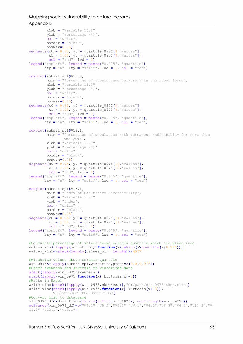
Mapping social vulnerability to natural hazards
Appendix B
Roman Breitfuss-Schiffer – UNIGIS MSc, University of Salzburg 65
xlab = "Variable 10.2",
ylab = "Percentage (%)",
col = "white",
border = "black",
boxwex=0.75)
segments(x0 = 0.95, y0 = quantile_0975[8,"values"],
x1 = 1.05, y1 = quantile_0975[8,"values"],
col = "red", lwd = 1)
legend("topleft", legend = paste("0.975", "quantile"),
bty = "n", lty = "solid", lwd = 1, col = "red")
boxplot(subset_sp1$V11.3,
main = "Percentage of subsistence workers \nin the labor force",
xlab = "Variable 11.3",
ylab = "Percentage (%)",
col = "white",
border = "black",
boxwex=0.75)
segments(x0 = 0.95, y0 = quantile_0975[9,"values"],
x1 = 1.05, y1 = quantile_0975[9,"values"],
col = "red", lwd = 1)
legend("topleft", legend = paste("0.975", "quantile"),
bty = "n", lty = "solid", lwd = 1, col = "red")
boxplot(subset_sp1$V12.1,
main = "Percentage of population with permanent \ndisability for more than
one year",
xlab = "Variable 12.1",
ylab = "Percentage (%)",
col = "white",
border = "black",
boxwex=0.75)
segments(x0 = 0.95, y0 = quantile_0975[10,"values"],
x1 = 1.05, y1 = quantile_0975[10,"values"],
col = "red", lwd = 1)
legend("topleft", legend = paste("0.975", "quantile"),
bty = "n", lty = "solid", lwd = 1, col = "red")
boxplot(subset_sp1$V13.1,
main = "Index of Healthcare Accessibility",
xlab = "Variable 13.1",
ylab = "Index",
col = "white",
border = "black",
boxwex=0.75)
segments(x0 = 0.95, y0 = quantile_0975[11,"values"],
x1 = 1.05, y1 = quantile_0975[11,"values"],
col = "red", lwd = 1)
legend("topleft", legend = paste("0.975", "quantile"),
bty = "n", lty = "solid", lwd = 1, col = "red")
#Calculate percentage of values above certain quantile which are winsorized
values_win<-lapply(subset_sp1, function(x) which(x>quantile(x,0.975)))
values_win1<-stack(lapply(values_win, length))/4037
#Winsorize values above certain quantile
win_0975<-lapply(subset_sp1,Winsorize,probs=c(0.0,0.975))
#Check skewness and kurtosis of winsorized data
stack(lapply(win_0975,skewness))
stack(lapply(win_0975,function(x) kurtosis(x)-3))
#Write in Excel
write.xlsx(stack(lapply(win_0975,skewness)),"C:/path/win_0975_skew.xlsx")
write.xlsx(stack(lapply(win_0975,function(x) kurtosis(x)-3)),
"C:/path/win_0975_kurt.xlsx")
#Convert list to dataframe
win_0975_df<-data.frame(matrix(unlist(win_0975), ncol=length(win_0975)))
colnames(win_0975_df)=c("V5.1","V5.2","V5.3","V6.1","V6.2","V6.3","V6.4","V10.2","V
11.3","V12.1","V13.1")
Mapping social vulnerability to natural hazards
Appendix B
Roman Breitfuss-Schiffer – UNIGIS MSc, University of Salzburg 66
#Define dataframe to update
ind_update<-ind
win_0975_df<-cbind(win_0975_df,Nr=ind_update$Nr)
#Update dataframe with winsorized data
ind_update[ ,c("V5.1","V5.2","V5.3","V6.1","V6.2",
"V6.3","V6.4","V10.2","V11.3","V12.1",
"V13.1")] <- list(NULL)
ind_update<-merge(ind_update,win_0975_df,by="Nr")
ind_update <- ind_update[colnames(ind)]
#NORMALIZATION
#-----------------------------------------------------------------
#Normalize dataframe
polarity_norm<-c("POS","POS","POS","POS","POS","POS","POS","POS","POS","POS",
"POS","POS","POS","POS","POS","POS","POS","POS","POS","POS",
"POS","NEG","POS","POS","POS","POS","POS","POS","NEG","NEG",
"POS","POS","POS","NEG","NEG")
ind_minmax<-normalise_ci(ind_update,c(3:37),polarity_norm,method=2)
ind_zscore<-normalise_ci(ind_update,c(3:37),polarity_norm,method=1,z.mean=0,
z.std=1)
write.xlsx(ind_minmax,"C:/path/ind_minmax.xlsx",
sheetName="ind_minmax")
write.xlsx(ind_zscore,"C:/path/ind_zscore.xlsx",
sheetName="ind_zscore")
#Convert list to dataframe
ind_minmax_temp<-ind_minmax
ind_minmax_temp$norm_method<-NULL
ind_minmax_df<-data.frame(matrix(unlist(ind_minmax_temp), ncol=35))
colnames(ind_minmax_df)=c("V1.1","V1.2","V1.3","V2.1","V2.2","V2.3","V3.1","V3.2",
"V4.1","V5.1","V5.2","V5.3","V6.1","V6.2","V6.3","V6.4",
"V6.5","V6.6","V7.1","V8.1","V9.1","V9.3","V9.4","V10.1",
"V10.2","V10.3","V10.4","V10.5","V10.6","V10.7","V10.8",
"V11.3","V12.1","V13.1","V14.1")
remove(ind_minmax_temp)
ind_zscore_temp<-ind_zscore
ind_zscore_temp$norm_method<-NULL
ind_zscore_df<-data.frame(matrix(unlist(ind_zscore_temp), ncol=35))
colnames(ind_zscore_df)=c("V1.1","V1.2","V1.3","V2.1","V2.2","V2.3","V3.1","V3.2",
"V4.1","V5.1","V5.2","V5.3","V6.1","V6.2","V6.3","V6.4",
"V6.5","V6.6","V7.1","V8.1","V9.1","V9.3","V9.4","V10.1",
"V10.2","V10.3","V10.4","V10.5","V10.6","V10.7","V10.8",
"V11.3","V12.1","V13.1","V14.1")
remove(ind_zscore_temp)
#Divide dataframe in susceptibility and lack of resilience domain
ind_minmax_SUS<-select(ind_minmax_df,V2.1,V2.2,V2.3,V3.1,V3.2,V4.1,V10.1,V10.2,
V10.3,V10.4,V10.5,V10.6,V10.7,V12.1)
ind_minmax_LoR<-select(ind_minmax_df,V1.1,V1.2,V1.3,V5.1,V5.2,V5.3,V6.1,V6.2,V6.3,
V6.4,V6.5,V6.6,V7.1,V8.1,V9.1,V9.3,V9.4,V10.8,V11.3,V13.1,
V14.1)
ind_zscore_SUS<-select(ind_zscore_df, V2.1,V2.2,V2.3,V3.1,V3.2,V4.1,V10.1,V10.2,
V10.3,V10.4,V10.5,V10.6,V10.7,V12.1)
ind_zscore_LoR<-select(ind_zscore_df,V1.1,V1.2,V1.3,V5.1,V5.2,V5.3,V6.1,V6.2,V6.3,
V6.4,V6.5,V6.6,V7.1,V8.1,V9.1,V9.3,V9.4,V10.8,V11.3,V13.1,
V14.1)
#Write in Excel
write.xlsx(ind_minmax_SUS, "C:/path/ind_minmax_SUS.xlsx",
sheetName="ind_minmax_SUS")
write.xlsx(ind_minmax_LoR, "C:/path/ind_minmax_LoR.xlsx",
sheetName="ind_minmax_LoR")
write.xlsx(ind_zscore_SUS, "C:/path/ind_zscore_SUS.xlsx",
sheetName="ind_zscore_SUS")
write.xlsx(ind_zscore_LoR, "C:/path/ind_zscore_LoR.xlsx",
sheetName="ind_zscore_LoR")
Mapping social vulnerability to natural hazards
Appendix B
Roman Breitfuss-Schiffer – UNIGIS MSc, University of Salzburg 67
#MULTIVARIATE ANALYSIS
#-----------------------------------------------------------------
#Calculate correlation
write.xlsx(cor(ind_minmax_SUS), "C:/path/Corr/corr_minmax_SUS.xlsx",
sheetName="corr_minmax_SUS")
write.xlsx(cor(ind_minmax_LoR), "C:/path/Corr/corr_minmax_LoR.xlsx",
sheetName="corr_minmax_LoR")
write.xlsx(cor(ind_zscore_SUS), "C:/path/Corr/corr_zscore_SUS.xlsx",
sheetName="corr_zscore_SUS")
write.xlsx(cor(ind_zscore_LoR), "C:/path/Corr/corr_zscore_LoR.xlsx",
sheetName="corr_zscore_LoR")
#Plot correlation matrix
col1<-colorRampPalette(rev(c("#67001F", "#B2182B", "#D6604D", "#F4A582",
"#FDDBC7", "#FFFFFF", "#D1E5F0", "#92C5DE",
"#4393C3", "#2166AC", "#053061")))
corrplot(cor(ind_minmax_SUS), type="lower", col=col1(200), tl.col="black",
tl.cex=1.2, tl.srt=45)
corrplot(cor(ind_minmax_LoR), type="lower", col=col1(200), tl.col="black",
tl.cex=1.2, tl.srt=45)
corrplot(cor(ind_minmax_SUS), method="number", type="lower", col=col1(200),
tl.col="black", tl.cex=1.2, tl.srt=45, number.cex=0.75)
corrplot(cor(ind_minmax_LoR), method="number", type="lower", col=col1(200),
tl.col="black", tl.cex=1.2, tl.srt=45, number.cex=0.75)
#Calculate VIF
#Write in Excel
y<-data.frame("y"=rep(1,4037))
y<-as.matrix(y)
reg_minmax_SUS<-lm(y~V2.1+V2.2+V2.3+V3.1+V3.2+V4.1+V10.1+V10.2+V10.3+V10.4+V10.5+
V10.6+V10.7+V12.1,ind_minmax_SUS)
write.xlsx(vif(reg_minmax_SUS), "C:/path/Corr/VIF_minmax_SUS.xlsx",
sheetName="VIF_minmax_SUS")
reg_minmax_LoR<-lm(y~V1.1+V1.2+V1.3+V5.1+V5.2+V5.3+V6.1+V6.2+V6.3+V6.4+V6.5+V6.6+
V7.1+V8.1+V9.1+V9.3+V9.4+V10.8+V11.3+V13.1+V14.1,ind_minmax_LoR)
write.xlsx(vif(reg_minmax_LoR), "C:/path/Corr/VIF_minmax_LoR.xlsx",
sheetName="VIF_minmax_LoR")
reg_zscore_SUS<-lm(y~V2.1+V2.2+V2.3+V3.1+V3.2+V4.1+V10.1+V10.2+V10.3+V10.4+V10.5+
V10.6+V10.7+V12.1,ind_zscore_SUS)
write.xlsx(vif(reg_zscore_SUS), "C:/path/Corr/VIF_zscore_SUS.xlsx",
sheetName="VIF_zscore_SUS")
reg_zscore_LoR<-lm(y~V1.1+V1.2+V1.3+V5.1+V5.2+V5.3+V6.1+V6.2+V6.3+V6.4+V6.5+V6.6+
V7.1+V8.1+V9.1+V9.3+V9.4+V10.8+V11.3+V13.1+V14.1,ind_zscore_LoR)
write.xlsx(vif(reg_zscore_LoR), "C:/path/Corr/VIF_zscore_LoR.xlsx",
sheetName="VIF_zscore_LoR")
#Elimination of Variables with high collinearity (r>0.8, VIF>5.0)
ind_minmax_SUS_updatecorr<-ind_minmax_SUS
ind_minmax_SUS_updatecorr["V2.1"]<-NULL
ind_minmax_LoR_updatecorr<-ind_minmax_LoR
ind_minmax_LoR_updatecorr[ ,c("V9.1","V9.3")]<-list(NULL)
ind_zscore_SUS_updatecorr<-ind_zscore_SUS
ind_zscore_SUS_updatecorr["V2.1"]<-NULL
ind_zscore_LoR_updatecorr<-ind_zscore_LoR
ind_zscore_LoR_updatecorr[ ,c("V9.1","V9.3")]<-list(NULL)
#Plot correlation matrix
corrplot(cor(ind_minmax_SUS_updatecorr), type="lower", col=col1(200),
tl.col="black", tl.cex=1.2, tl.srt=45)
corrplot(cor(ind_minmax_LoR_updatecorr), type="lower", col=col1(200),
tl.col="black", tl.cex=1.2, tl.srt=45)
corrplot(cor(ind_minmax_SUS_updatecorr), method="number", type="lower",
col=col1(200), tl.col="black", tl.cex=1.2, tl.srt=45, number.cex=0.75)
corrplot(cor(ind_minmax_LoR_updatecorr), method="number", type="lower",
col=col1(200), tl.col="black", tl.cex=1.2, tl.srt=45, number.cex=0.75)

Mapping social vulnerability to natural hazards
Appendix B
Roman Breitfuss-Schiffer – UNIGIS MSc, University of Salzburg 68
#Calculate correlation
#Write in Excel
write.xlsx(cor(ind_minmax_SUS_updatecorr),
"C:/path/Corr/update_corr_minmax_SUS.xlsx",
sheetName="update_corr_minmax_SUS")
write.xlsx(cor(ind_minmax_LoR_updatecorr),
"C:/path/Corr/update_corr_minmax_LoR.xlsx",
sheetName="update_corr_minmax_LoR")
write.xlsx(cor(ind_zscore_SUS_updatecorr),
"C:/path/Corr/update_corr_zscore_SUS.xlsx",
sheetName="update_corr_minmax_SUS")
write.xlsx(cor(ind_zscore_LoR_updatecorr),
"C:/path/Corr/update_corr_zscore_LoR.xlsx",
sheetName="update_corr_minmax_LoR")
#Calculate VIF
#Write in Excel
reg_minmax_SUS_updatecorr<-lm(y~V2.2+V2.3+V3.1+V3.2+V4.1+V10.1+V10.2+V10.3+V10.4+
V10.5+V10.6+V10.7+V12.1,ind_minmax_SUS_updatecorr)
write.xlsx(vif(reg_minmax_SUS_updatecorr),
"C:/path/Corr/update_VIF_minmax_SUS.xlsx",
sheetName="update_VIF_minmax_SUS")
reg_minmax_LoR_updatecorr<-lm(y~V1.1+V1.2+V1.3+V5.1+V5.2+V5.3+V6.1+V6.2+V6.3+V6.4+
V6.5+V6.6+V7.1+V8.1+V9.4+V10.8+V11.3+V13.1+V14.1,
ind_minmax_LoR_updatecorr)
write.xlsx(vif(reg_minmax_LoR_updatecorr),
"C:/path/Corr/update_VIF_minmax_LoR.xlsx",
sheetName="update_VIF_minmax_LoR_")
reg_zscore_SUS_updatecorr<-lm(y~V2.2+V2.3+V3.1+V3.2+V4.1+V10.1+V10.2+V10.3+V10.4+
V10.5+V10.6+V10.7+V12.1,ind_zscore_SUS_updatecorr)
write.xlsx(vif(reg_zscore_SUS_updatecorr),
"C:/path/Corr/update_VIF_zscore_SUS.xlsx",
sheetName="update_VIF_zscore_SUS")
reg_zscore_LoR_updatecorr<-lm(y~V1.1+V1.2+V1.3+V5.1+V5.2+V5.3+V6.1+V6.2+V6.3+V6.4+
V6.5+V6.6+V7.1+V8.1+V9.4+V10.8+V11.3+V13.1+V14.1,
ind_zscore_LoR_updatecorr)
write.xlsx(vif(reg_zscore_LoR_updatecorr),
"C:/path/Corr/update_VIF_zscore_LoR.xlsx",
sheetName="update_VIF_zscore_LoR")
#Principle Component Analysis - Factor Analysis
#Write in Excel
PCA_SUS<-prcomp(ind_zscore_SUS_updatecorr)
summary(PCA_SUS)
eigenvalues_SUS<-get_eig(PCA_SUS)
loadings_SUS<-t(t(PCA_SUS$rotation)*sqrt(eigenvalues_SUS$eigenvalue))
write.xlsx(loadings_SUS, "C:/path/PCA/PCA_SUS.xlsx",
sheetName="loadings_SUS")
write.xlsx(get_eig(PCA_SUS), "C:/path/PCA/PCA_SUS.xlsx",
sheetName="eigen_SUS", append=TRUE)
fviz_eig(PCA_SUS, choice="eigenvalue")
PCA_LoR<-prcomp(ind_zscore_LoR_updatecorr)
summary(PCA_LoR)
eigenvalues_LoR<-get_eig(PCA_LoR)
loadings_LoR<-t(t(PCA_LoR$rotation)*sqrt(eigenvalues_LoR$eigenvalue))
write.xlsx(loadings_LoR, "C:/path/PCA/PCA_LoR.xlsx",
sheetName="loadings_LoR")
write.xlsx(get_eig(PCA_LoR), "C:/path/PCA/PCA_LoR.xlsx",
sheetName="eigen_LoR", append=TRUE)
fviz_eig(PCA_LoR, choice="eigenvalue")
#Varimax-rotation factors=5 based on eigenvalues >1.0 and total represented
Variance >60%
#Write in Excel
PCA_SUS_rotated<-principal(ind_zscore_SUS_updatecorr,rotate="varimax",nfactors=5,
scores=TRUE)
Mapping social vulnerability to natural hazards
Appendix B
Roman Breitfuss-Schiffer – UNIGIS MSc, University of Salzburg 69
write.xlsx(PCA_SUS_rotated$loadings[1:13,], "C:/path/PCA/PCA_SUS.xlsx",
sheetName="varimax_SUS_loadings", append=TRUE)
write.xlsx(PCA_SUS_rotated$Vaccounted, "C:/path/PCA/PCA_SUS.xlsx",
sheetName="varimax_SUS_Var", append=TRUE)
PCA_LoR_rotated<-principal(ind_zscore_LoR_updatecorr,rotate="varimax",nfactors=5,
scores=TRUE)
write.xlsx(PCA_LoR_rotated$loadings[1:19,], "C:/path/PCA/PCA_LoR.xlsx",
sheetName="varimax_LoR_loadings", append=TRUE)
write.xlsx(PCA_LoR_rotated$Vaccounted, "C:/path/PCA/PCA_LoR.xlsx",
sheetName="varimax_LoR_Var", append=TRUE)
#Define final set of indicators/variables
#Normalized
ind_minmax_SUS_final<-ind_minmax_SUS_updatecorr
ind_minmax_LoR_final<-ind_minmax_LoR_updatecorr
ind_zscore_SUS_final<-ind_zscore_LoR_updatecorr
ind_zscore_LoR_final<-ind_zscore_LoR_updatecorr
#Write in Excel
write.xlsx(ind_minmax_SUS_final, "C:/path/Ind_minmax_SUS_final.xlsx",
sheetName="ind_minmax_SUS_final")
write.xlsx(ind_minmax_LoR_final, "C:/path/Ind_final/Ind_minmax_LoR_final.xlsx",
sheetName="ind_minmax_LoR_final")
write.xlsx(ind_zscore_SUS_final, "C:/path/Ind_final/Ind_zscore_SUS_final.xlsx",
sheetName="ind_zscore_SUS_final")
write.xlsx(ind_zscore_LoR_final, "C:/path/Ind_final/Ind_zscore_LoR_final.xlsx",
sheetName="ind_zscore_LoR_final")