Scholars' Mine Scholars' Mine

Masters Theses Student Theses and Dissertations

1971

A triangular element for numerical solutions of axisymmetric A triangular element for numerical solutions of axisymmetric

conduction problems in cylindrical coordinates conduction problems in cylindrical coordinates

Prafulla Chandra Mahata

Follow this and additional works at: https://scholarsmine.mst.edu/masters_theses

Part of the Mechanical Engineering Commons

Department: Department:

Recommended Citation Recommended Citation Mahata, Prafulla Chandra, "A triangular element for numerical solutions of axisymmetric conduction problems in cylindrical coordinates" (1971). Masters Theses. 5488. https://scholarsmine.mst.edu/masters_theses/5488

This thesis is brought to you by Scholars' Mine, a service of the Missouri S&T Library and Learning Resources. This work is protected by U. S. Copyright Law. Unauthorized use including reproduction for redistribution requires the permission of the copyright holder. For more information, please contact scholarsmine@mst.edu.

A TRIANGULAR ELEMENT FOR NUMERICAL SOLUTIONS OF

AXISYMMETRIC CONDUCTION PROBLEMS IN

CYLINDRICAL COORDINATES

by

PRAFULLA CHANDRA MAHATA, 1947-

A

THESIS

Presented to the Faculty of the Graduate School of the

UNIVERSITY OF MISSOURI-ROLLA

In Partial Fulfillment of the Requirements for the Degree

MASTER OF SCIENCE IN MECHANICAL ENGINEERING

1971

Approved by

(}_J., ~ 61J-, (Advisor) & (! M Jl\ r fh c<(b ~

(}

ABSTRACT

The triangular element is one of the many suitable

elements which are used in finite difference methods as

ii

applied to conduction heat transfer. Such elements find

many applications in conduction problems in Cartesian

coordinates. This work proposes a new triangular element

for axisymmetric conduction problems in cylindrical

coordinates. The validity and workability of the networks

formed by the proposed triangular elements are strengthened

by selected examples. The work is completed by the

application of the triangular element to an industrial

problem having irregular boundaries. The results are

compared with the solution obtained by the finite element

method.

ACKNOWLEDGEMENTS

The author wishes to extend sincere thanks and

appreciation to his advisor, Dr. R.O. McNary, for

the initial motivation and valuable suggestions,

guidance and encouragement throughout the course of

this thesis.

The author is grateful to Dr. R.L. Davis, Dr. H.D.

Keith and Mr. K. Hambacker for providing the finite

element solution in Chapter Vr and to Dr. D.C. Look for

his critical review of the work.

Thanks are due also to Mrs. Connie Hendrix for

typing the thesis.

iii

TABLE OF CONTENTS

ABSTRACT . .

ACKNOWLEDGEMENTS

LIST OF ILLUSTRATIONS

LIST OF TABLES .

LIST OF SYMBOLS

I. INTRODUCTION

II. DEVELOPMENT OF THE TRIANGULAR NETWORK

A. Geometric Factors for a Rectangular Element . . .

B. Geometric Factors for a Triangular Element

III. VALIDITY OF THE TRIANGULAR NETWORK IN CYLINDRICAL COORDINATES

Page

ii

. iii

vi

.viii

ix

1

10

10

12

16

A. Parameters in the Geometric Factor . 16

B. Deviation in the Geometric Factors for the Triangular Element . 19

IV. COMPARISON OF SOLUTIONS USING THE PROPOSED TRIANGULAR ELEMENT WITH SOLUTIONS BY OTHER METHODS . . . . . . . 33

A. An Infinitely Long Hollow Cylinder . 33

i. Analytical Method

ii. Rectangular Network Method

iii. Triangular Network Method

B. A Circular Fin With Rectangular Profile . . . .

i. Analytical Method

ii. Rectangular Network Method

iii. Triangular Network Method

34

36

38

45

45

48

50

iv

TABLE OF CONTENTS (Continued)

C. A Solid Cylinder of Finite Length .

i. Analytical Method . .

ii. Rectangular Network Method .

iii. Triangular Network Method

V. AN INDUSTRIAL APPLICATION .

VI. CONCLUSION.

BIBLIOGRAPHY •

VITA . . . .

APPENDICES

A. LENGTHS OF PERPENDICULAR BISECTORS OF A TRIANGULAR ELEMENT IN CYLINDRICAL

v

Page

56

57

60

61

66

76

78

79

80

COORDINATE SYSTEM . . . . . . . . . . . . 80

B. AN ALGEBRAIC APPROACH TO RELATE THE THERMAL CONDUCTANCES OF RECTANGULAR AND TRIANGULAR ELEMENTS IN CYLINDRICAL COORDINATES . . • . . . . . . . . . . 8 3

Figure

1

2

3

4

5

6

7

8

9

10

11

12

13

14

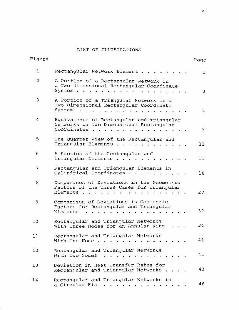
LIST OF ILLUSTRATIONS

Rectangular Network Element .

A Portion of a Rectangular Network in a Two Dimensional Rectangular Coordinate System .

A Portion of a Triangular Network in a Two Dimensional Rectangular Coordinate System

Equivalence of Rectangular and Triangular Networks in Two Dimensional Rectangular Coordinates .

One Quarter View of the Rectangular and Triangular Elements .

A Section of the Rectangular and Triangular Elements .

Rectangular and Triangular Elements in Cylindrical Coordinates .

Comparison of Deviations in the Geometric Factors of the Three Cases for Triangular Elements .

Comparison of Deviations in Geometric Factors for Rectangular and Triangular Elements

Rectangular and Triangular Networks With Three Nodes for an Annular Ring

Rectangular and Triangular Networks With One Node .

Rectangular and Triangular Networks With Two Nodes

Deviation in Heat Transfer Rates for Rectangular and Triangular Networks .

Rectangular and Triangular Networks in a Circular Fin

vi

Page

3

3

3

5

11

11

18

27

32

34

41

41

43

46

vii

LIST OF ILLUSTRATIONS (Continued)

Figure Page

15

16

17

18

19

20

21

Al

Bl

Temperature Distribution in a Circular Fin by Three Methods .

Comparison of Deviations in Heat Transfer Rates for Rectangular and Triangular Network Methods •

Rectangular and Triangular Networks in a Finite Solid Circular Cylinder .

Temperature Distribution in a Solid Cylinder of Finite Length by Three Methods

Deviations in the Dimensionless Temperatures by Two Methods for a Solid Cylinder of Finite Length .

Section of the Bottom of a Reaction Vessel .

Use of the Triangular Network in an Irregular Weld Joint .

A Triangular Element in Two Dimensional Cylindrical Coordinates

A Sectional View of the Rectangular and Triangular Elements

55

55

58

65

65

67

69

80

84

Table

I

II

III

IV

v

VI

LIST OF TABLES

Percentage Deviations in Resultant Geometric Factors for Triangular Elements .

Percentage Deviations in Geometric Factors for Rectangular and Triangular Elements.

Temperatures and Heat Transfer Rates for an Infinitely Long Hollow Cylinder Using Three Methods of Solution

Temperatures and Heat Transfer Rates for a Circular Fin by Three Methods of Solution .

Temperatures and Heat Transfer Rates for a Solid Cylinder by Three Methods of Solution .

Comparison of the Finite Difference and Finite Element Methods .

viii

Page

25

31

42

54

64

72

Q

k

A

T

n

s

K

x,y

r,z

a,b,c,d,e,g,h,L

E

i

I

am

lm

r*,z*

d*,e*,L*

Q*

T*

h

A.*

r' J;!

lX

LIST OF SYMBOLS

heat transfer rate

conductivity

area of heat transfer

temperature

direction

geometric factor

thermal conductance

rectangular coordinates

cylindrical coordinates

increment

lengths

percentage deviation

index of irregularity for one triangle

index of irregularity for a group of triangles

arithmetic mean

logarithmic mean

dimensionless coordinates

dimensionless lengths

dimensionless heat transfer rate

dimensionless temperature

convective heat transfer coefficient

dimensionless eigenvalue

spherical coordinates

percentage difference

1

I. INTRODUCTION

In many situations mathematical techniques are

adequate to obtain analytical solutions of the problems

encountered in many fields of Science and Engineering.

However, in attacking irregular and complicated bodies,

the mathematics may become extremely tedious. Cases

are not rare wherein analytical solutions are impossible

with the application of existing techniques. In such

cases numerical methods are used successfully. Digital

computers have added extra advantage and feasibility to

the numerical methods in recent years. These methods

have wide applicibility in the field of heat transfer by

conduction in the calculation of the temperature distri-

bution and heat transfer rates. Elements of several

shapes such as rectangular, triangular, hexagonal and

polar are commonly used in numerical methods. The present

interest is in triangular elements which have the advan-

tage of fitting into irregular geometries.

Elements are employed to give a finite difference

form to the Fourier law of heat conduction which is stated

as

Q = -kA aT an I ( 1)

where Q, k, A, T and n are the heat transfer rate, conduc-

tivity, area of heat transfer, temperature and direction

of heat transfer, respectively. Using the rectangular

element (Fig. 1) for preliminary illustration, the

finite difference form of Eq. (1) is given by

Q = -kA I'::.T/I'::.n,

2

( 2)

where I'::.T and l'::.n are incremental quantities. Related to

the finite difference form of the law of conduction heat

transfer are the geometric factorS and the thermal conduc­

tance K of the element, which are defined by [1]

S = A/l'::.n, K = kA/I'::.n, ( 3 )

respectively.

in

Introducing Eqs. (3) into Eq. (2), results

Q = -K I'::.T. ( 4 )

Recognizing Q as the current, 1/K as the resistance and

I'::.T as the potential difference, Eq. (4) is analogous to

Ohm's law in electrical technology. This analogy leads to

the possible network representation of any physical problem

in conduction heat transfer. A network is defined to

consist of heat conducting rods which represent the

elements and which are connected to each other in a parti­

cular way depending on the type of the elements. The

junctions are called nodes of the network. Before intra-

ducing the actual subject matter of the present work,

some common types of networks and related facts are

3

T T+L'IT

r----...., I I

Q -~ ~- Q

A ~ Representative Rod A__,"---- ~

~ L'ln Associated Material

Fig. 1. Rectangular Network Element

y

. . ·= 1 2 3

. . . r 4 5 6 y

L . . 7 118 lg

V- L'lx --.!1'

L-------------------------~-x

Fig. 2. A Portion of a Rectangular Net­work in a Two Dimensional Rectangular Coordinate System

X

Fig. 3. A Portion of a Triangular Net­work in a Two Dimensional Rectangular Coordinate System

4

discussed to serve as ground work.

A. Common Networks

In two dimensional Cartesian coordinates the commonly

used networks are rectangular (Fig. 2), triangular (Fig. 3),

hexagonal, polar, etc.

It is known that the rectangular network solutions

approach the analytical results, as the dimensions of

the biggest element in the network approach zero (~x ~ 0,

~y ~ 0). The triangular network involves multiple direc-

tions and variable areas of heat transfer (Fig. 3). It

may be difficult to prove by the direct method of letting

the elemental dimension approach zero that the triangular

network solutions approach the analytical results. How-

ever, the validity of the triangular network has been

established by Dusinberre(l] with the aid of an indirect

method. A brief outline of this method is given here to

link the present work with Dusinberre's. Dusinberre's

analysis established the equivalence of rectangular and

triangular networks in two dimensional rectangular

coordinates by showing the equality of the thermal conduc-

tances of the elements of the two networks. Consequently,

the validity of the triangular network has been proved.

The element AXYZ (Fig. 4) of a rectangular network in

two dimensional rectangular coordinates is composed of the

-Q

Fig. 4.

y

N

B

-h Q -

Equivalence of Rectangular and Triangular Networks in Two Dimensional Rectangular Coordinates

5

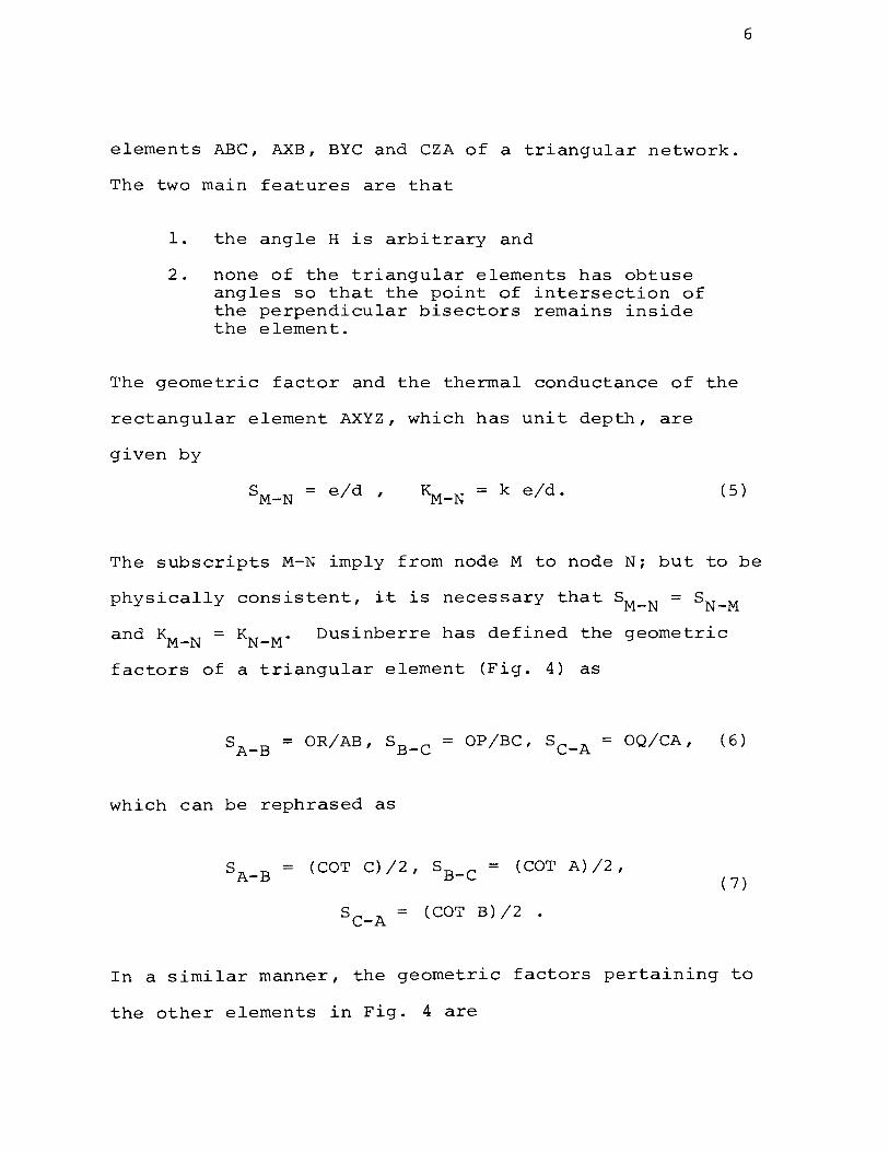
elements ABC, AXB, BYC and CZA of a triangular network.

The two main features are that

1. the angle H is arbitrary and

2. none of the triangular elements has obtuse angles so that the point of intersection of the perpendicular bisectors remains inside the element.

The geometric factor and the thermal conductance of the

rectangular element AXYZ, which has unit depth, are

given by

6

SM-N = e/d , K_ = k e/d. -M-N ( 5 )

The subscripts M-N imply from node M to node N; but to be

physically consistent, it is necessary that SM-N = SN-M

Dusinberre has defined the geometric

factors of a triangular element (Fig. 4) as

SA-B = OR/AB, SB-C = OP/BC, SC-A = OQ/CA, (6)

which can be rephrased as

SA-B = (COT C)/2, SB-C = (COT A)/2, (7)

SC-A = (COT B)/2 .

In a similar manner, the geometric factors pertaining to

the other elements in Fig. 4 are

7

SA-X= (COT D)/2, SC-Y = (COT F)/2,

( 8 ) SC-Z = (COT G)/2.

By the electrical network analogy the total thermal

conductance KT of all the triangular elements in Fig. 4

is the resultant of the thermal conductances of the

representative heat conducting rods ZC, AC, CY, CB, AB,

AX and is given by

( 9)

which simplifies to

KT = (k/2) [(COT A+ COT F) (COT B +COT G)/(COT A

(10) +COT F +COT B +COT G) +COT C +COT D).

Further simplification with the aid of trigonometric

relations results in [1]

KT = k e/d. (11)

Comparison of Eqs. ( 5) and ( 11) shows that

(12)

which proves that the triangular elements are equivalent

to the rectangular element for arbitrarily chosen direction

of heat transfer (angle H being arbitrary) and with

suitably defined geometric factors for the triangular

elements.

8

The triangular network discussed so far is in two

dimensional rectangular coordinates and thus it is

applicable to plane bodies only. This limitation points

out the need for a triangular network in two dimensional

cylindrical coordinates (r,z), which can handle irregular

axisymmetric bodies. Unfortunately, the work of

Dusinberre in the rectangular coordinate system has not

been extended to the cylindrical coordinate system.

Reid [2] determined analytically the steady state

temperature distribution for the special case of a

30-degree right triangle with temperatures specified on

the boundary. The solution is in two dimensional

rectangular coordinates. The method is so involved that

the author says, "To fully appreciate the difficulty

involved, one should try to solve some other case such

as a 31-degree right triangle."

Lancoz [3] and Garabedian [4] indicate that for

irregular boundaries, the boundary value problem of even

simple differential operators become practically unman­

ageable if the aim is to arrive at an analytical solution.

The triangle in general form is an example of a region

for which an explicit solution to the Dirichlet problem

in closed form is presently unknown.

9

It appears that little work has been done on the

triangular element in cylindrical coordinates. The

present work provides a convenient and feasible

definition of the geometric factors for the triangular

network in two dimensional cylindrical coordinates (r,z).

The validity of the network is established by proving

that its accuracy is comparable to the rectangular

network in cylindrical coordinates and that the accuracy

improves as the size of the elements is decreased. Three

examples further strengthen the reliability and the

workability of such triangular networks. Another example

of industrial interest is chosen to highlight all the

major aspects of the application of the triangular net­

work in two dimensional cylindrical coordinates.

10

II. DEVELOPMENT OF THE TRIANGULAR NETWORK

To develop the triangular network in two dimensional

cylindrical coordinates (r,z), the prime task is to define

the geometric factors of the triangular element in a

suitable way. Three feasible definitions are given in

this chapter and analysis using these definitions are

considered. Before considering the triangular element,

two alternate ways of defining geometric factors for a

rectangular element in two dimensional cylindrical

coordinates are discussed because of their use in succeeding

chapters.

A. Geometric Factors for a Rectangular Element

The rectangular element with section AXYZ (Fig. 5),

as shown in two dimensional cylindrical coordinates, forms

a complete ring around the z-axis. Any radial plane

intersecting the element forms a rectangular cross section.

On the basis of the arithmetic mean area, the geomet-

ric factor SR of the rectangular element with section

AXYZ (Fig.6) is defined as

ne(r. + r )/(r - r.), l 0 0 l

( 13)

where r., r and e are the internal and the external radii l 0

and the length of the element, respectively.

Fig. 5.

z

Fig. 6.

z

y

I I

I B I I

r A X

One Quarter View of the Rectangular and Triangular Elements

r 0

A Section of the Rectangular and Triangular Elements

r

11

12

Introducing

d = r - r. 0 1

(14)

in Eq. (13), yields

= ne(2r. +d)/d. 1

On the basis of the logarithmic mean area, the

geometric factor SR of the rectangular element is

defined as (5]

= 2ne/ln(r /r.). 0 1

B. Geometric Factors for a Triangular Element

The triangular element with section ABC (Fig.5)

(15)

(16)

is a ring around the z-axis and results in a triangular

cross section with the intersection of any radial plane.

The perpendicular bisectors OP, OQ and OR intersect at a

common point 0 inside the element as shown in Fig. 6.

The geometric factors for triangular element ABC can be

written in a manner similar to Eqs. (6) as

5A-B = (Area of surface of revolution by OR)/AB,

5 B-C = (Area of surface of revolution by OP)/BC, (17)

5 c-A = (Area of surface of revolution by OQ)/CA.

13

The areas of surfaces of revolutions by OR, OP and OQ

are considered in three different possible ways, which

give rise to three possible definitions for the geometric

factors.

Case 1: Areas Based on Mid-Radii of Perpendicular Bisectors

In this case the areas across OR, OP and OQ are

the exact areas of the cylindrical surfaces containing OR,

OP and OQ. So Eqs. (17) give

SA-B = 2TI[(r0 +rR)/(2AB)]OR, SB-C = 2TI[(r0 +rp)/(2BC)]OP,

(18)

where the subscript of the radius r implies radius to

that point.

Case 2: Areas Based on Common Radius of Perpendicular Bisectors

In this case the areas of heat transfer are based

on the radius corresponding to the common point 0 of the

perpendicular bisectors. The geometric factors for the

triangular elements are then obtained from Eqs. (17) as

(19)

14

Case 3: Areas Based on Mid-Radii of Conducting Rods

Considering the areas across the perpendicular

bisectors based on the mid-radius of each side, the

geometric factors for the triangular element are obtained

from Eq. (17) as

SA-B = 2n(rR/AB)OR, SB-C = 2n(rp/BC)OP, SC-A=2n(rQ/CA)OQ.

(20)

It is noted that although the exact area is employed

in case 1, the definition of the geometric factors are

not unique. Thus it is required to consider the equiva­

lence of the rectangular and the triangular elements in

a two dimensional cylindrical coordinate system, as is

exhibited in the case of the rectangular coordinate system

in Eq. (12). Using the definitions of the geometric

factors in case 1, an analysis of the equivalence of the

rectangular and the triangular elements is given in

Appendix B. The results of the analysis show that the

exact equivalence does not exist in the cylindrical

coordinate system. Any possibility of equivalence, con-

sidering case 2 and case 3, is discussed later. However,

the exact equivalence of the two networks is not required.

For example, the network of rectangular elements based

on two different definitions of the geometric factors,

15

the arithmetic mean area and the log mean area, are

non-equivalent. However, they are both used for general

engineering practice.

The immediate task is then to analyze the deviations

in the three definitions of the geometric factor for the

triangular element as compared to the geometric factor

for the rectangular element based on either the arithmetic

mean area or the logarithmic mean area.

III. VALIDITY OF THE TRIANGULAR NETWORK IN CYLINDRICAL COORDINATES

The geometric factors and hence the thermal

conductances are the basic parameters which govern the

temperature distribution and the heat transfer rates

obtained by the finite difference method. Thus any

16

1naccuracy associated with the geometric factor causes

errors in the temperature distribution and heat transfer

rates. In this chapter the deviation in the geometric

factor for the triangular element with respect to the

geometric factor for the rectangular element is analyzed

for all the cases (cases 1,2 and 3). The geometric

factor for the rectangular element based on the arithmetic

mean area is taken as the basis of comparison for con-

venience. However, a simple relation can be used to alter

the basis for comparison. In order to consider the

geometric factor for a triangular element, it is essential

to specify the shape of the element. This shape is a

major factor in the possible variation of the geometric

factor.

A. Parameters in the Geometric Factor

Fig. 7 illustrates a rectangular element with section

AXYZ in cylindrical coordinates, which is composed of

triangular elements with sections ABC, AXB, BYC and CZA.

17

The perpendicular bisectors and the necessary dimensions

are shown in the figure. The shape and location of the

triangular element can be completely specified by the

parameters r • 1 d 1 l

e, g and h. Dividing these by

the dimensionless parameters are obtained as

r. * = r.jr. = 1, d* d/r., e* = e/r., l l l l l

g* = g/r., h* = h/r .. l l

r. , l

( 21)

The dimensionless parameter d* is taken as the measure

of the size of the rectangular element and representative

of the size of the triangular elements. However, the

shapes of the triangular elements are dictated by all the

four parameters d*, e*, g* and h*. A single index is

introduced here to represent all possible shapes of the

triangular element and to give an indication of the

irregularity. Such an index of a triangle can be defined

as the sum of the absolute values of the three differences

of the angles in that triangle. Thus the value of the

index i ranges from 0 to TI as the irregularity of a

triangle increases with the restriction of no obtuse

angles. Another index I for a group of triangles may be

defined as the sum of the individual indices of all the

triangles in that group. The expression for I is given by

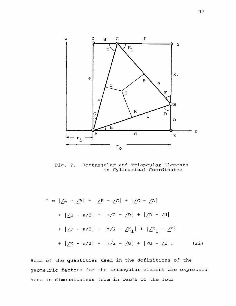
z z g c f

e

h

~------~~--~--------------------~~----- r l= r i ----t r -d ------.~r 0

Fig. 7. Rectangular and Triangular Elements in Cylindrical Coordinates

r = I/A - /BI + I/B - /cl + l!c - /AI

+ I/H- n/21 + [n/2 - /DI + I/D - /HI

18

+ I/E - n/21 + ln/2 - /GI + I/G - /EI. (22)

Some of the quantities used in the definitions of the

geometric factors for the triangular element are expressed

here in dimensionless form in terms of the four

19

dimensionless independent parameters d*, e*, g* and h*

as follows:

/F =arc tan[(d*-g*)/(e*-h*)],

/Kl = TI/2 - /F, /G = arc tan(g*/e*),

/E = TI/2 /G, /H = arc tan(h*/d*),

/D = TI/2 - /H, /A = TI/2 - (/H + /G)

b* = g*/sin G, c* = h*/sin H,

a* 2 2 1/2

= (b* +c* -2b*c*cosA)

/B = arc sin(b*sin A/a*), /C = arc sin(c*sin A/a*),

OR* = (c*/2)COT C, OP* = (a*/2)COT A, OQ* = (b*/2)COT B,

r * = r.* + (c*/2)sin(C-H)/sin C, 0 l

r * = r.* + d*/2, R 1 r * = r.* + d*/2 + g*/2, p l

r * = r.* + g*/2. Q l ( 2 3)

The geometric factor SR for the rectangular element

with section AXYZ based on the arithmetic mean area

method, as given in Eq. (15), can be expressed in dimen-

sionless form as

S * = ne*(2r.* + d*)/d*, R 1

where

B. Deviation in the Geometric Factors for the Triangular Element

(24)

( 2 5)

20

In this section a comparison is made between the

geometric factors for the triangular element and the

geometric factor for the rectangular element defined on

the basis of the arithmetic mean area. The three cases

for the definition of the geometric factors, as discussed

in the last chapter, will now be considered.

Case 1: Areas Based on Mid-Radii of Perpendicular Bisectors

In this case the geometric factors for the triangular

element with section ABC obtained from Eqs. (18) with the

aid of the trigonometric relations in Appendix B can be

written in dimensionless forms as

(26)

The dimensionless expressions for the necessary geometric

factors for the other triangular elements in Fig. 7 are

(27)

The dimensionless resultant thermal conductance of the

triangular elements is obtained from Eq. (9) as

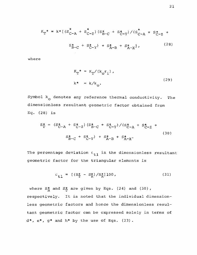
where

K * T

k* = k/k . 0

21

( 2 8)

(29)

Symbol k0

denotes any reference thermal conductivity. The

dimensionless resultant geometric factor obtained from

Eq. ( 2 8) is

S* T

(30)

The percentage deviation Etl in the dimensionless resultant

geometric factor for the triangular elements is

( 31)

where s~ and s; are given by Eqs. (24) and (30),

respectively. It is noted that the individual dimension-

less geometric factors and hence the dimensionless resul-

tant geometric factor can be expressed solely in terms of

d*, e*, g* and h* by the use of Eqs. (23).

22

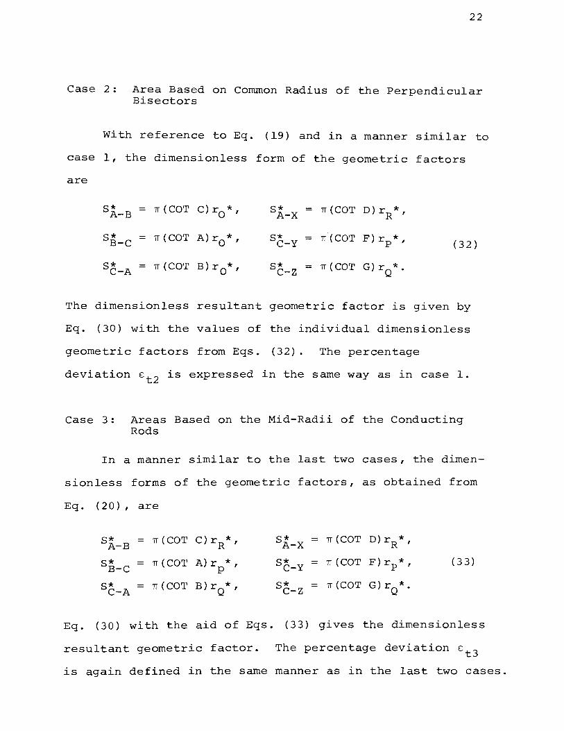
Case 2: Area Based on Common Radius of the Perpendicular Bisectors

With reference to Eq. (19) and in a manner similar to

case 1, the dimensionless form of the geometric factors

are

SA-B = 7T(COT C) r 0 *, SA-X = 7T(COT D)rR * I

s:B-c = 1T(COT A)r0 * SC-Y = 1T(COT F)rp*, , ( 32)

SC-A = 1T(COT B)r0*, sc-z = 7T(COT G)rQ * 0

The dimensionless resultant geometric factor is given by

Eq. (30) with the values of the individual dimensionless

geometric factors from Eqs. (32). The percentage

deviation Et2 is expressed in the same way as in case 1.

Case 3: Areas Based on the Mid-Radii of the Conducting Rods

In a manner similar to the last two cases, the dimen-

sionless forms of the geometric factors, as obtained from

Eq. ( 2 0) , are

SA-B = 7T(COT C)rR * SA-X = 1T(COT D)rR * , ,

SB-C = 7T(COT A)r * SC-Y = 1T(COT F)rp*, ( 3 3) p ,

SC-A = 1T(COT B)rQ * sc-z = 7T(COT G)rQ * , 0

Eq. (30) with the aid of Eqs. (33) gives the dimensionless

resultant geometric factor. The percentage deviation Et3

is again defined in the same manner as in the last two cases.

23

The following method was employed in order to compute

the percentage deviations in the three cases for various

shapes of the triangular elements.

a. Ten suitable values (0.04, 0.08, ... , 0.40) of d* were

chosen to represent the size of the triangular

elements.

b. For each value of d*, ten suitable values (0.04,

0.08, ... ,0.40) of e* were used. These values alter

the shape of the rectangular and the triangular

elements.

c. For every value of e*, nine values of g* were taken

at intervals of one-tenth of d*. For each value of

g* nine values of h* were also considered at an

interval of one-tenth of e*.

The total number of shapes considered by the above

method is 8100. The shapes having obtuse angle were

omitted for the reason previously stated. Table I lists

the results of the computation giving the percentage

deviations in all the three cases corresponding to a few

particular shapes of the triangular elements. From the

results of all possible shapes under study, it is observed

that the case 3 gives the least percentage deviation for

most of the considered shapes of the triangular elements.

The list in Table I includes only those sets which have

d*

0.04

0.08

0.12

0.16

0.20

0.24

24

Table I. Percentage Deviations in Resultant Geometric Factors for Triangular Elements

e* g* h* I E:tl E:t2 E:t3

0.04 0.004 0.004 9.999 -0.046 -0.090 -0.002

0.04 0.020 0.008 7.585 -0.083 -0.160 -0.006

0 .12 0.004 0.108 11.082 -0.398 -0.794 -0.002

0.04 0.016 0.004 8.709 -0.049 -0.092 -0.006

0.08 0.008 0.016 9.530 -0. 16 0 -0.313 -0.007

0.08 0.040 0.016 7.585 -0.170 -0.320 -0.022

0.24 0.008 0.216 11.082 -0.781 -1.558 -0.007

0.04 0.024 0.004 10.081 -0.038 -0.051 -0.029

0.08 0.108 0.024 9.566 -0.142 -0.271 -0.014

0.12 0.060 0.024 7.585 -0.262 -0.479 -0.048

0.04 0. 012 0.004 11.146 -0.030 -0.036 -0.027

0.08 0.060 0.008 8.960 -0.097 -0.137 -0.062

0.16 0.144 0.144 9. 317 -0.175 -0.334 -0.024

0.16 0.080 0.032 7.585 -0.358 -0.637 -0.082

0.40 0.064 0.360 10.847 -1.064 -2.085 -0.067

0.08 0.048 0.008 10.0 81 -0.105 -0.113 -0.109

0. 12 0.180 0.048 9.602 -0. 219 -0.405 -0.036

0.16 0.120 0.016 7.570 -0.225 -0.326 -0.131

0.08 0.020 0.032 10.889 -0.128 -0. 19 8 -0.063

0.12 0.100 0.036 9.417 -0.271 -0.388 -0.175

0.24 0.216 0.024 9.182 -0.284 -0.521 -0.048

0.24 0.120 0.048 7.585 -0.558 -0.950 -0.171

0.08 0.024 0.008 11.146 -0.087 -0.083 -0.102

0.12 0.072 0.012 10.081 -0.194 -0.184 -0.231

25

Table I (continued)

d* e* g* h* I Etl Et2 Et3

0.28 0.28 0.252 0.028 9.181 -0.332 -0.603 -0.062

0.28 0.140 0.056 7.585 -0.661 -1.105 -0.2 2 4

0.12 0.028 0.060 10.787 -0.215 -0.326 -0.112

0.16 0.140 0.016 9.263 -0. 2 87 -0.277 -0.332

0.32 0.24 0.288 0.048 9. 42 5 -0.374 -0.671 -0.079

0.28 0.160 0.028 7.337 -0.469 -0.640 -0.308

0.12 0.032 0.036 10.983 -0.199 -0.256 -0.158

0.16 0.096 0.016 10.081 -0. 301 -0.261 -0.389

0.36 0.28 0.324 0.056 9 .3 87 -0.446 -0.799 -0.094

0.32 0.180 0.032 7.368 -0.553 -0.745 -0.374

0.12 0.036 0.012 11.146 -0.163 -0.137 -0.216

0.20 0.180 0.020 9.320 -0.412 -0.358 -0.525

0.40 0.40 0.360 0.040 9.181 -0.475 -0.840 -0.111

0.36 0.200 0. 0 36 7.392 -0.640 -0.852 -0.444

0.16 0.040 0.064 10.889 -0.303 -0.401 -0.225

0.24 0.200 0.072 9.417 -0.648 -0.779 -0.588

26

the minimum and the maximum percentage deviations in

the preferred case 3 and the minimum and the maximum

values of the index I. All the extreme values are under­

lined. The percentage deviations in the numerous other

shapes are not listed mainly due to the unpredictable

nature of the percentage deviations in terms of the

index I and because of space limitations. However,

Fig. 8 is used to represent all the results of the com­

putation in the form of regions of percentage deviations

corresponding to the representative size d* of the

triangular element.

The results in Table I and Fig. 8 indicate the

following:

1. The resultant geometric factor for the triangular

elements approaches the geometric factor for the

rectangular element as the size of the elements

of the network decreases. This establishes the

validity of the triangular network.

2. There is no preferred shape of the triangular

elements.

3. The geometric factors formulated in the case 3

yield better results. It is noted that case

1 based on exact areas does not give the

most accurate results. Thus case 3 is preferred

z 0 H E-t ~ H

4.0

1.0

27

:> rLl 0.1 Q

rLl

~ E-t z rLl u ~ rLl P-i

Ii-I 0

rLl :::>

~ .01

7

The figures in the shaded regions are the corresponding values of element size d*

Case 1

9

INDEX I

11 7

Case 2

9

INDEX I

11 7

Case 3

9

INDEX I

Fig. 8. Comparison of Deviations in The Geometric Factors of the Three Cases for Triangular Elements

28

for further use in triangular networks. Case 3

gives a rapid decrease in the percentage deviations

in the resultant geometric factor with a decrease

in d*. This is evident in Fig. 8. Also this for-

mulation of the geometric factors is the simplest

among the three cases under consideration.

The percentage deviation in the resultant geometric

factor for the triangular elements (considering case 3)

with respect to the geometric factor for the rectangular

element based on the logarithmic mean area will now be

analyzed for comparison. This analysis was done indirectly

by the following methods.

From Eq. (15) the dimensionless geometric factor

S* for the rectangular element based on the arithmetic R am

mean area is given by

S* = ne*(2r~ + d*)/d*, Ram 1

and from Eq. (16) the dimensionless geometric factor

S* based on the logarithmic mean area is Rlm

= 2ne*/ln[(r~ + d*)/r~]. l l

(34)

(35)

The percentage deviation Earn in the geometric factor

based on the arithmetic mean area with respect to that

based on the logarithmic mean area is given by

E = [ (S* am R am SR_ ) /S:R ] 10 0 I

lm lm

which, combined with Eqs. (34) and (35), reduces to

E am [(1/2 + 1/d*)ln(l + d*)-1]100.

The case 3 version of Eq. (31) gives the percentage

( 3 6)

( 3 7)

deviation Et3 in the dimensionless resultant geometric

factor for the triangular elements with respect to the

geometric factor for the rectangular element based on

the arithmetic mean area. The rearranged form of the

above mentioned equation is

= S*/S* - 1. T R am

Eq. (36) is rephrased as

E /100 = S* /S* - 1. am R Rl am m

( 3 8)

(39)

29

The percentage deviation Et in the resultant geometric

factor for the triangular elements (considering case 3)

with respect to the geometric factor for the rectangular

element using the logarithmic mean area method is given

by

= [(s;- sR )/SR_ 1100, lm lm

(40)

which is rearranged as

st = [S*/S* - 1]100. T Rlm

Egs. (38) and (39) jointly give

S*/S* T Rlm

which, when introduced into Eg. (41), yields

E am

30

( 41)

(42)

( 4 3)

Using Table I, the minimum and the maximum values of st

were computed and result listed in Table II. Fig. 9

shows the variations of sam and Et versus the element

size d*. It illustrates the following important facts.

1. Et is smaller than sam everywhere within the

range of d* under consideration and for all of

the 8100 shapes. Corresponding to d* = 0.40,

the maximum values of s and st are 0.942 and am

0.831 percent, respectively. As these deviations

are comparable, the workability of the triangular

network using formulations of case 3 may be

assumed.

2. Both the minimum and the maximum values of Et

decrease rapidly with a decrease in the size (d*)

of the element. This indicates that the deviation

approaches zero as the element size decreases.

d*

0.04

0.08

0.12

0.16

0.20

0.24

0.28

0.32

0.36

0.40

Table II. Percentage Deviations in Geometric Factors for Rectangular and Triangular Elements

E:t E:

am minimum maximum

0.013 0.007 0. 011

0.049 0.020 0.042

0 .107 0.045 0.093

0.183 0.074 0.159

0.277 0.102 0.241

0.385 0.154 0.337

0.507 0.175 0.445

0.642 0.253 0.563

0. 7 87 0.262 0.693

0.942 0.364 0.831

31

E am

E am For rectangular elemen using arithmetic mean area

Et For triangular element

.001~--~--~--~---L---L---L--~--~L---L---~--~ 0.00 0.08 0.16 0.24 0. 32 0.40

ELEMENT SIZE d*

Fig. 9. Comparison of Deviations in Geometric Factors for Rectangular and Triangular Elements

32

IV . COMPARISON OF SOLUTIONS USING THE PROPOSED TRIANGULAR ELEMENT WITH SOLUTIONS BY

OTHER METHODS

Since case 3 is the preferred formulation, hence-

forth all the triangular networks are based on that

33

formulation. Three examples have been selected to illus-

trate the workability of the triangular network by com-

parison with the rectangular network (arithmetic mean

area method) and with analytical methods. An equal

number of nodes are employed wherever possible in both

the rectangular and the triangular network methods to

obtain fair comparison. For convenience in the analysis,

steady state conduction problems with constant thermal

conductivity for the case of no heat sources or sinks

will be considered. These complicating factors may be

treated by the usual methods.

The first example in the series will now be illus-

trated using the three different methods.

A. An Infinitely Long Hollow Cylinder

Fig. 10 shows a cross section of an annular ring

which is a part of an infinitely long hollow cylinder.

This will be treated as a one dimensional problem.

Using the constants T. and T as the inside and the out-l 0

side temperatures, the purpose now is to find the

z

I I

I . I I t

I e X

L

I I I

I I I I

I I I I

I l I

I I I I . . . . .

I 1 I 2 I 3 I

I I I I

I I I I

I I I

I I

y

c r. .. l

I. d/2-

r 0 z

z

I

z

T. l

Fig. 10. Rectangular and Triangular Networks with Three Nodes for an Annular Ring

T 0

temperature distribution and the heat transfer rate by

34

the analytical method, by the rectangular network method

and by the triangular network method.

i. Analytical Method

The differential equation governing the heat con-

duction is given by

35

d dTa dr (r dr) = 01 ( 4 4)

where the subscript a denotes the analytical method.

The boundary conditions are

T (r.) = T. 1 a 1 1 Ta(ro) =To. ( 4 5)

The dimensionless temperature T* and heat transfer rate a

Q* per unit length are given as a

T* = 1 - ln r*/ln r * a o 1

Q* = (T~- T*)/[(l/2TI)ln(l + d*)) a 1 o

where the dimensionless quantities are defined by

T* a

(T -T )/{T.-T ) I a o 1 o

T* = (T -T )/(T.-T ) 0 0 0 l 0

Q* = Q /[r.ke*(T.-T ) ] 1 a a 1 1 o

T~ = (T.-T )/(T.-T) I l l 0 l 0

r* = rjr. 1 l

r* 0

r jr. 1 0 l

d* = [(r -r.)/2]/r. 1 0 l . l

e* = /3 d*/2.

( 4 6)

( 4 7)

( 4 8)

Noting that r* = 1 + 2d* 1 T~ = 1 and T* = 01 the dimen-o l 0

sionless temperatures T~1 ~ T~2 ~ etc. 1 and the heat

transfer rate per unit length are computed from Eqs. (46)

36

and {47) corresponding to the values of d* and r*. The

results are given in Table III,page 42.

ii. Rectangular Network Method

A rectangular network is formed for the annular

ring as shown in Fig. 10 and an energy balance is

performed at each of the three nodes to obtain

( 4 9)

The thermal conductances for the rectangular elements by

the arithmetic mean area method are

KX-1 = k 2Tie{r. + dl4)l(dl2) 1 l

Kl-2 = k 2Tie(r. + 3 dl 4 ) I ( dl 2 ) I l

(50)

K2,...3 = k 2Tie(r1 + 5 dl4) I (dl2) I

K3-Y = k 2Tie(r. + 7 dl4)l(dl2). l

Inserting the values of the thermal conductances from

Eqs. (50) in Eqs. {49), solving for the dimensionless

temperatures and dividing numerator and denominator by

ri' yield

T* 1

T* 2

T* 3

= [ (l+d*/4)T! + (1+3d*/4)T2]/(2+d*) I

= [ (1+3d*/4)Ti+(l+5d*/4)T3*]/(2+2d*) I

[(1+5d*/4)T2+(1+7d*/4)T~]/(2+3d*).

37

(51)

The above set of equations was solved for the dimen-

sionless temperatures using the Gauss-Seidel iterative

method [6] with suitable values of d*. The iteration

process was terminated when the maximum difference in

the values of any of the unknown temperatures, obtained

by the successive iterations, was 0.5 x 10-6 • The heat

transfer rate in per unit length at the interior surface

can be expressed as

Q (52)

Introducing KX-l from Eqs. (50) in Eq. (52) and non­

dimensionalizing, yields

Q* = 2TI [ {1 + d*/4) /(d*/2)] (T! - Ti). (53)

In a similar manner the expression for heat transfer rate

at the outer surface can be obtained. The percentage

deviation El in the temperature at node 1 with respect to

the analytical case based on the maximum temperature

range is given in dimensionless form as

(54)

38

Similar expressions are used to find s 2 and s 3 corres­

ponding to node 2 and node 3, respectively. The percen-

tage deviation Eq in the heat transfer rates with respect

to the analytical method takes the dimensionless form

E = [Q*- Q*)/Q*]lOO. q a a (55)

The nodal dimensionless temperatures with the corresponding

percentage deviations and the heat transfer rates with the

corresponding percentage deviations are listed in Table

III.

iii. Triangular Network Method

A triangular network is shown in Fig. 10. For con-

venience in analysis, as many regular triangular elements

as possible are used. The nodes are located at the same

radial positions as in the rectangular network. An

energy balance at each node in terms of the dimensionless

temperatures is performed to obtain

KP-l(Ti- T!) + KQ-l(Tf- Ti) + K2-l(T2-T!)+K3-l

(T) - Ti) = 0 I

K (T* - T*) + K (T~ - T*) + K (T* - T*) + 1-2 1 2 Q-2 1 2 R-2 0 2

K (T* - T*) + K. 3 (T2*- T*3 ) + KR 3 (T*- T*3 ) + 1-3 1 3 2- - 0

K (T* - T*) = 0 S-3 0 3 I

(56)

39

where the thermal conductances are given by

KP-1 = k2TI (r.+dl4) (el2) I (dl2), l

KQ-1 = k2TI(r.+dl4) (el3)ld, K2-1 = k2TI(r.+3dl4) (2el3)ld, l l

K3-l = k2TI (r. +d) (el3) ld, KQ-2 = k2TI(r.+dl2) (el3)ld, l l

KR-2 = k 2 'IT ( r . + 3 dl 2) ( e I 3 ) I d , K3-2 = k2TI(r.+5dl4) (2el3)ld, l l

KR-3 = k2TI(r.+7dl4) (el3)ld, KS-3 = k2TI(r.+7dl4) (el2)l(dl2). l l

(57)

Introducing the values of the thermal conductances into

Eqs. (56) and solving for the dimensionless nodal tern-

peratures, yield

Ti = [3(1 + d*I4)Tf + (1 + d*I4)Ti + 2(1 + 3d*I4)T2

+ (1 + d*)T)11(7 + 7d*l2),

T2 = [2(1 + 3d*I4)Ti +(1 +d*I2)Ti + (1 + 3d*I2)T0

*

+ 2(1 + 5d*I4)T 3*]1(6 + 6d*),

T) = [(1 + d*)Ti + 2(1 + 5d*I4)T2 + (1 + 7d*I4)T0

*

+ 3(1 + 7d*I4)T *]1(7 + 2ld*l2). 0

(57 a)

In a manner similar to the rectangular network method,

these equations are solved for the dimensionless temperatures.

40

The heat transfer rate in per unit length Q is given

by

which, when simplified and nondimensionalized with the

values of the thermal conductances from Eqs. (57), reduces

to

Q* = (TI /3- ) [3(1 + d*/4) (T~-T*) + (1 + d*/4) (T~-T*) l 1 l 1

+ (l + d*/2) (T~- T2)]. (59)

Similarly the dimensionless heat transfer rate out per

unit length is obtained. The percentage deviations in

the dimensionless temperatures and the heat transfer

rates compared to the analytical case are calculated as

in the last case and are compiled in Table III.

In addition,for the same ratio r /r. this example 0 l

was solved using one node and two nodes in a manner

similar to the method just outlined for three nodes.

Figs. 11 and 12 illustrate the networks which were used.

The results are also in Table III. The graphs of E: q

versus the size of the element for the rectangular method

and for the triangular method with one, two and three

nodes are shown in Fig. 13. From Table III and Fig. 13

the following conclusions can be made.

z

I· z

z

z

d

I (.1.,_--------------------__ ....,.,:'L---------- --------_ ~'•) y X I l I

I I I I e

j____P~.~------~------~~------~~--------~· S r

0

Fig. 11. Rectangular and Triangular Networks with One Node

Q I I I I

. R

I _ I x ./_-_---~------~ .. ·r---- -----~~----- _____ ...J,•J Y

2

e

I. d

Fig. 12. Rectangular and Triangular Networks with Two Nodes

s

..I

T 0

41

I ' .

'

Table III. Temparatures and Heat Transfer Rates for an Infinitely Long Hollow Cylinder Using Three Methods of Solution

r /r.=l.36 0 l

d* Methods (N)

Analytical

0.36 Rectangular (1)

Triangular

Analytical

0.24 Rectangular ( 2)

Triangular

Analytical

0.18 Rectangular

( 3) Triangular

T * 1 T *

2

.46172

.46186

.46186

.63143 .30043

. 6 3150 .30047

.63133 .30068

.71974 .46172

. 719 76 . 4617 5

. 719 6 8 .46180 -~'-

N: Number of Nodes

Q* E T * El E E3 3 in out 2 in

20.43414

20.47507 20.47505 0.014 .200

20.51501 20.51500 0. 014 .396

20.43414

20.45242 20.45235 0.007 0.005 . 0 89

20.47623 20.47620 -0.010 0.026 .206

.22267 20.43414

.22269 20.44455 20.44431 0.002 0.003 .002 .051

.22279 20.45963 20.45950 -0.006 0.008 .012 .125

q

out

.200

. 39 6

. 0 89

.206

.051

.12 5

I

I

~

N

z 0 H E-t r::C H

0.4

0.3

> r:£1 0.2 Q

r:£1

~ E-t z r:£1 u p:; r:£1 P-1

0.1

r /r. = 1.36 0 l

SYMBOLS

El RECTANGULAR NETWORK

& TRIANGULAR NETWORK

0.0 0.1 0.2 0.3

ELEMENT SIZE d*

Fig. 13. Deviation in Heat Transfer Rates for Rectangular and Triangular Networks

43

0.4

44

1. The temperatures obtained by the rectangular and

the triangular networks have comparable percentage

deviations for every size of element under consider-

ation. For example, corresponding to d* = 0.24

values of El are 0.007 and -0.010 for the rectangu-

lar and triangular networks, respectively. These

deviations are well within the requirements of

general engineering accuracy.

2. The percentage deviation E for the triangular q

element has a maximum value of 0.396 compared to

0.200 for the rectangular element, corresponding

to d* = 0.36. The value of E for the triangular q

element is within general engineering accuracy,

although it is almost double the value for the

rectangular element. The trend of the graphs

indicate that the triangular network gives a more

rapid decrease in E with a decrease in the element q

size as compared to the rectangular network. This

trend further indicates the validity of the

triangular element, because the error diminishes

as the network becomes finer.

The second example is subject to convective

boundary conditions.

B. A Circular Fin with Rectangular Profile

Fig. 14 illustrates the geometry of the fin under

consideration. The results of the triangular network

will again be compared with those of a rectangular

network and with the analytical method. The fin is

assumed to have an insulated end, base temperature and

the ambient temperatures of Ti and Tf, respectively,

and a constant convective heat transfer coefficient h

from the surface of the fin. The problem is analyzed

in one dimension.

i. Analytical Method

The differential equation governing the heat

conduction in the fin is [7]

d [k A(r) dT] dr dr

(60)

where the area for conduction A(r) and the differential

area dAs for convection are

A(r) = 2nre and dAs = 2(2nr dr). ( 61)

Introducing the dimensionless temperature T* and radius

r* as

and r* = r /r. , l

( 6 2)

45

z

z

z

t z

~ e

L:

Q I I I

Ti~

r. l

I

r 0

h,Tf

1

d/2

h,Tf

I. d j Fig. 14. Rectangular and Triangular

Networks in a Circular Fin

46

INSULATED

3'

INSULATED

Eq. (60) becomes

where

d 2T* dT* 2 2 + r* - m* r* T* = 0 dr*2 dr*

m* 2 = [2h/(ke)]r. 2 . l

Eq. (63) is a Bessel's equation of order zero. Its

( 6 3)

(64)

solution [5] with the associated boundary conditions

T* (r.*) = T.*, l l

is

dT*(r *) 0

dr* = 0, (65)

/II (m*r.*)K (m*r *)+K (m*r.*)I (m*r *)] 0 l 1 0 0 l 1 0'

(66)

47

where I 0 , I 1 and K0 , K1 are modified Bessel's functions

of first and second kind of order zero and one, respecti-

vely. The dimensionless temperatures T *, T * and T * al a2 a3

(subscript a is for analytical case) corresponding to the

dimensionless radii r 1 *, r 2 * and r 3* can now be obtained.

The heat transfer rate Q * (i.e. heat lost by the fin) a

through the base of the fin is

K (m*r *)]/[I (m*r.*)K (m*r *)+K (m*r.*) 1 0 0 l 1 0 0 l

r 1 (m*r0

*)] (67)

where the dimensionless expressions for Q * and e* are a

Q * = Q /[kr. (T.-Tf)], a a 1 1

e*= e/r .. 1

( 6 Sa)

(68b)

The temperatures and the heat transfer rates are given

in Table IV for three values of m* for a fin of a fixed

geometry.

ii. Rectangular Network Method

48

The network for this method is also shown in Fig. 14.

To find the nodal temperatures, an energy balance at each

node is performed using the dimensionless temperatures,

as defined in Eq. (62). The result is

K 2

_ 3

( T 2

* -T 3

* ) + 2 h [ 2 TI ( r i + lld/ 8) ( d/ 4) ] ( T f * -T 3 *) = 0 ,

(69)

The thermal conductance KX-l is

KX-l = k[2n(ri+d/4)e/(d/2)], (70)

49

where d = 2el/3. The other thermal conductances are

obtained in like manner and are inserted into Eqs. (69)

to yield expressions for the dimensionless temperatures.

The result is

T1

* = [2(lld* + li4)Ti* + 2(lld* + 3I4)T 2 *+m* 2 (l+d*l2)

(d*I2)Tf*ll12(lld*+ll4)+2(lld*+314)+m* 2 (l+d*l2)

(d*l2)] I

T 2 * = [2 (lld*+314) T1 *+2 (lld*+514)T 3 *+m* 2 (l+d*) (d*l2)

T f * ] I [ 2 ( 1 I d * + 3 I 4 ) + 2 ( 1 I d * + 5 I 4 ) +m * 2 ( 1 + d * ) ( d *I 2 ) ] ,

T3

* = [2 (lld*+514)T 2 *+m* 2 (l+lld*l8) (d*I4)Tf*JI

[2 (lld*+514)+m* 2 (l+lld*l8) (d*l4)],

where d* = dlr .. l

( 71)

The above equations are solved for the dimensionless

temperatures. The heat transfer rate in at the base is

written as

which, when simplified and nondimensionalized with the

aid of Eq. (70), reduces to

Q* = 21Te* [2 (lld*+ll4) (Ti *-T 1 *) +m*2

(l+d*IB) (d*l4)

(T. *-T *) ] l f I

( 7 3)

50

where Q* is defined in Eq. (68a). The dimensionless

heat loss by convection Q* is similarly found to have

the expression

Q* = 2'1Te*m*2

[ (l+d*/8) (d*/4) (Ti*-Tf*)+(l+d*/2) (d*/2)

( 7 4)

Eqs. (73) and (74) will give the same value of Q*. The

percentage deviations s 1 , s 2 and s3

in the dimensionless

temperatures are obtained from Eq. (54). The percentage

deviations s in the dimensionless heat transfer rates q

are obtained by using Eqs. (55) 1 ( 7 3) 1 ( 7 4) 1 and are com-

piled in Table IV.

iii. Triangular Network Method

Fig. 13 illustrates the triangular network used.

The nodes are positioned at the same radius as in the

rectangular network method for direct comparison of

temperatures. Regular triangular elements are selected

so that the conductances can be computed with ease. The

representative element size d is taken as

d = 2e//3 . ( 7 5)

Performing an energy balance at each node in terms of

the dimensionless temperatures gives

51

+h [2TT (ri+dl2) (3dl4)] (Tf*-Tl *) = 0,

Kl 2(Tl*-T2*)+KQ 2(T.*-T2*)+K (T3*-T *)+K (T*-T*) - - 1 ~-2 2 3-2 3 2

5dl4) (di2)+2TT(ri+lldl8) (dl4)] (Tf*-T3

*) = 0.

The thermal conductances are

~- 1=k[2TT (ri+dl4) (el2) I (dl2)],

KQ_ 1=k[2TT(ri+dl4) (el3)ld],

K2

_1

=k[2TT (ri+3dl4) (2el3)ld].

( 7 6)

(77)

Introducing the expressions for all the conductances into

Eqs. (76) and solving the resulting equations yields the

expressions

Tl* = [2 (lld*+li4)T.*+(213) (lld*+li4)T.*+(413) (lid* 1 1

+314)T2

*+(213) (lld*+l)T3

*+m*2

(l+d*l2) (3d*I4)Tf]

1[2 (lld*+ll4)+(213) (lld*+ll4)+(413) (lld*+314)

+m * 2 ( 1 +d * 12 > ( 3d* I 4 > ] ,

52

T;= L (413) (lld*+314)Tl *+ (213) (lld*+li2)Ti *+2 (lid*

+ 5 I 4 ) T 3 * + ( 2 I 3 ) ( 1 I d * + 5 I 4 ) T 3

* +m * 2 ( 1 + d * ) ( 3d* I 4 )

Tf*JI[ (413) (lld*+314)+(213) (lld*+ll2)+

2(lld*+SI4)+(213) (lld*+5l4)+m* 2 (l+d*) (3d*l4)],

T 3 * = [(213) (lld*+l)T 1 *+(213) (lld*+5I4)T2

*+2(lld*+

5I4)T 2 *+m* 2 ( (1+5d*l4) (d*l2)+(l+lld*l8) (d*l4))

Tf*JI[(213) (lld*+l)+(213) (lld*+SI4)+2(lld*+

5l4)+m* 2 ((1+5d*l4) (d*l2)+(l+lld*l8) (d*l4))].

( 7 8)

Assigning values to d* and m*, the above equations were

solved for the dimensionless nodal temperatures. The

heat transfer rate in at the base is given by

(dl4)+2n(r.+dl4) (dl2)] (T.-Tf). 1 1

(79)

The expressions for thermal conductances are used

from Eqs. (77) and the definition of Q* is introduced,

giving

Q* = ne* [2 (lld*+ll4) (Ti *-T1 *)+ (213) (lld*+ll4) (T_i-Ti)

+(213) (lld*+ll2) (Ti*-T 2 *)+m* 2 ( (l+d*l8) (d*l4)

+ (l+d*l4) (d*l2)) (Ti *-Tf*)]. (80)

In a similar manner, the dimensionless heat loss by

convection Q* is found to have the expression

Q* = ne*m*2

[ (l+d*/8) (d*/4) (Ti*-Tf*)+ (l+d*/4) (d*/2)

(Ti*-Tf*)+(l+d*/2) (3d*/4) (T 1*-Tf*)+(l+d*)

(3d*/4) (T 2*-Tf*)+(l+5d*/4) (d*/2) (T 3*-Tf*)+

(l+lld*/8) (d*/4) (T 3*-Tf)]. ( 81)

53

The percentage deviations s 1 , s 2 , s 3 in the dimensionless

temperatures are evaluated using relations similar to

Eq. (54) . The percentage deviations E in the dimension­q

less heat transfer rates are obtained by Eq. (55) . These

results are listed in Table IV.

The following conclusions can be drawn from the

results:

1. The graph in Fig. 15 shows that the temperatures,

obtained by the rectangular and triangular network

methods, are very close. For example when d*=0.4 and

m*=l.5, the dimensionless temperatures T2 * having

maximum deviation are 0.69635 and 0.70533 for the

rectangular and triangular networks,respectively.

2. It is observed in Fig. 16 that the percentage

deviation in the heat transfer rate for the

triangular network method is 0.333% for m*=0.5.

Table IV. Temperatures and Heat Transfer Rates for a Circular Fin by Three Methods of Solution

d*=0.4

Q* m* Methods T * 1 T * 2 T * 3 E:l E:2 E:3

in loss in

Analytical .97071 .95446 .94968 .40905

0.5 Rectangular .97057 .95463 .94972 .40946 . 409 43 -.014 . 017 .004 .099

Triangular .97172 .95575 .95001 . 410 41 .41041 .101 .129 .033 .333

Analytical . 89 42 8 .83816 .82092 1.47795

LO Rectangular . 89 50 4 .83928 . 82 2 2 8 1. 48500 1.48498 .076 . 112 .136 .478

Triangular .89909 . 84 361 .82371 1. 499 41 1. 49940 .481 .545 .279 1. 453

Analytical . 79 7 59 .69360 .66218 2.88132

1.5 Rectangular .79954 .69635 .66541 2.91391 2.91389 .195 .275 .323 1.131

Triangular .80694 .70533 .66902 2.97788 2.97788 . 9 35 1.173 . 6 84 3.351 ~--

E: q

loss

0.093

.333

. 4 7 7

1.453

1.130

3.351

I I

Ul of:>.

l.o--~---r--~~--.---r-~--~--~~~

m*=0.5

iC 8 0. 9 ji:l p:; ~ 8

~ ji:l 1=4 ~ ji:l

8 0. 8 U) U) ji:l H z d*:::::0.4 0 H SYMBOLS U)

z ji:l :8 0. 7 0 ANALYTICAL H Cl I

~ -A G RECTANGULAR

& TRIANGULAR

0.6L-_J---L--J---~~~~---L--J-~

1.0 1.2 1.4

DIMENSIONLESS RADIUS r*

Fig. 15. Temperature Distribution in a Circular Fin by Three Methods

1.6

z 0 H 8 ~ H

> ji:l Cl

ji:l ~ ~ 8 z ji:l u p:; ji:l 1=4

4.0~--.----,---,,---~--~--~--~

I / d* = 0.4

I I SYMBOLS

~ El RECTANGULAR

o. o5l 8 TRIANGULAR

0.02~--~--~--~----~--~--~--~

0.0 0.5 1.0 1.5

PARAMETER m*

Fig. 16. Comparison of Deviation in Heat Transfer Rates for Rectangular and Triangular Network Methods

V1 V1

However, for higher values of m* the temperature

gradient at the base of the fin is large and this

introduces more error in both the rectangular and

the triangular network methods. The percentage

deviation in the triangular network method can be

maintained within required workable limits

although it is found to be almost three times

that of the rectangular network method.

Thus far only one dimensional examples have been

discussed. A two dimensional problem will now be

analyzed.

C. A Solid Cylinder of Finite Length

In the last two examples, the triangular network

forces the heat transfer to take place in an unnatural

direction. This may be responsible for the superior

accuracy of the rectangular network method in examples

A and B. Thus to investigate the suitability of the

triangular network in a two dimensional example is the

purpose of this discussion.

The assumptions, stated earlier, are employed for

this example. The following dimensions are selected

for convenience.

d = r /3, 0

e = 13 d/2, L = 4e. (82)

56

The cylindrical surface and one of the faces are main-

tained at a constant temperature T . The second face 0

has the impressed axisymmetric temperature distribution

f(r) as shown in Fig. 17. A suitable expression for

f(r) will be chosen later.

i. Analytical Method

The differential equation governing the heat con-

duction in the solid finite cylinder is [ 7]

( 8 3)

The boundary conditions are

T(r,O) = T 1 T(r,L) = f(r) 1 T(r lz) = T 1 0 0 0

T(r,z) is finite. (84)

57

The temperature T0

is constant.

ties

The dimensionless quanti-

P* = r /L, 0

are introduced where T f is the value of f(O). re

(85)

Separa-

tion of variables was used to solve this boundary value

problem. The result is

T*(r*,z*) = J0

(A1

*r*)sinh(P*A 1*z*)/sinh(P*A 1*L*),

(86)

z T=f (r)

I

L I 5 I 6

.1. - L -I

8 J

r 0

z

w v u s

Fig. 17. Rectangular and Triangular Networks in a Finite Solid Circular Cylinder

58

J

T 0

r

Q

59

if f(r) is taken as

( 87)

The symbol A1 * is the first eigenvalue of the characteris­

tic equation

( 8 8)

and J 0 is the Bessel's function of the first kind of

order zero. The dimensionless temperatures are evaluated

by Eq. (86) with suitable values of r* and z* and are

denoted by Ta*· The heat transfer rate in Qa through the

top face of the cylinder (z=L) is given by

Q = k fro l! a 8z

0

• 2nrdr,

which has the dimensionless form

2 Jl 8T* Q * = (2n r /L) -~-* r* dr*, a 0 O oZ

where Q * is a

' . ClT* bt . d f E Subst1tut1ng Clz*' o a1ne rom q.

and integrating, yields

( 86) , into Eq.

(89)

( 9 0)

( 91)

(90)

The values of A1 * and J 1 (A 1 *) are available in standard

tables of Bessel's functions.

ii. Rectangular Network Method

The network for this method is shown in Fig. 17.

An energy balance is again performed at each node and

the conductances are expressed in terms of d and e.

When the values of the conductances are introduced into

60

the set of energy balance equations, the result in terms

of the dimensionless temperatures is

T * 1

T * 3

T * 5

T * 7 T*

8

T * 2

(93)

These equations are solved for the dimensionless tempera-

ture where TA*, TB*, Tc* and T0 * are defined by Eqs. (87)

and (85). The dimensionless heat transfer rate Q* across

the section I-I (Fig. 17) is found in a manner similar to

the last two examples. The expression is

61

Q* = ('IT/6)[2(T *-T1*)+16(T *-T *)+32(T *-T *)+15(T*-T*)] A B 2 C 3 C o

(9 4a)

Similarly, the dimensionless heat transfer rate across

the section J-J is found to be

( 9 4b)

The dimensionless heat transfer rate is defined in a

manner similar to Eq. (91). The percentage deviations

E in the dimensionless temperatures are obtained by using

expressions similar to Eq. (54). The percentage

deviations E in the dimensionless heat transfer rates are q

evaluated by using Eq. (55). The results of the computa-

tion are given in Table V.

iii. Triangular Network Method

The network, as shown in Fig. 17, is constructed

such that the total number of nodes is 10, compared to 9

in the rectangular network. All the nodes except the

nodes 45, 55 and 65 are positioned in identical locations

for direct comparison of the temperatures with the

rectangular network method. The thermal conductances

are again easily expressed in terms of d and e. The

simplification of the non-dimensional form of the set of

energy balance equations results in

T * 7

T * 8

62

(95)

where TA*, TB*, Tc*, TD* and T0

* are defined by Eqs. (87)

and (85) The above equations were solved for the nodal

temperatures. The dimensionless heat transfer rate Q*

across the section I-I (Fig. 17) is given by

(T *-T *)+28(T *-T *)+36(T *-T *)+88(T *-T *) C 2 C 3 D 3 D o .

(96a)

Similarly, the expression for the dimensionless heat

transfer rate Q* across the section J-J is found to be

63

Q* = (n/12) [88TD*+40T3 *+176T65 *+104T9 *+32T 8 *+3T7*].

(96b)

The percentage deviations in the dimensionless temperatures

and in the heat transfer rates in Eqs. (96a) and (96b)

are evaluated in a manner similar to the rectangular net­

work method. The results are given in Table V. Figs.l8

and 19 illustrate the temperature distribution and the

percentage deviations in the temperatures which result

from the calculations.

The following conclusions can be drawn from this

example.

1. The percentage deviations in the dimension­

less temperatures obtained by the triangular

network method are smaller than those obtained

by the rectangular network method. The maximum

percentage deviation E is -0.344% for the

triangular network as compared to 1.422% for

the rectangular network method.

2. Table V gives the percentage deviation in the

heat transfer rate as 3.210% for the triangular

network method, whereas for the rectangular

method the figure is -0.899%. They are com­

parable values.

d/r =1/3 0

Table V. Temperatures and Heat Transfer Rates for a Solid Cylinder by Three Methods of Solution

64

Node Position Analytical Rectangular Triangular

No. r* z* T a * T* E: T* E:

1 0 3/4 0.49360 0.50782 1. 422 0.49541 0.181

2 2/6 3/4 0.41742 0.43037 1.295 0.41737 -0.005

3 4/6 3/4 0.22385 0.23101 0.716 0.22411 0.026

4 0 2/4 0.23483 0.24797 1.314 0.23238 -0.245

45 1/6 2/4 0.22548 0.22204 -0.344

5 2/6 2/4 0.19859 0.21033 1. 17 4

55 3/6 2/4 0.15731 0.15706 -0.02 5

6 4/6 2/4 0.10650 0.11297 0.647

65 5/6 2/4 0.05204 0.05224 0.020

7 0 1/4 0.09387 0.10103 0.716 0.09340 -0.047

8 2/6 1/4 0.07938 0.08572 0. 6 34 0.07890 -0.048

9 4/6 1/4 0.04257 0.04605 0.348 0.04256 -0.001

Sections Q * Q* E: Q* E: a q q

I-I 11.38635 11.28405 -0.898 11.75191 3.211 J-J 11 .2 8 3 9 4 - 0 . 8 9 9 11.75189 3. 210

1.0~--~----~----~--~----~--~

~ p:; ::>

~ ~ 0. 6 P-t :2:: ~ 8

U)

U) 0 4 ~ . H z 0 H U) :z;

~ 0. 2 H 0

d/r = 1/3 0 SYMBOLS

0 ANALYTICAL

G RECTANGULAR

Q.J I ~ I ~ 0 1/6 2/6 3/6 4/6 5/6

DIMENSIONLESS RADIUS r*

Fig. 18. Temperature Distribution in a Solid Cylinder of Finite Length by Three Methods

1

~ 2.or-----.------.-----.------r-----,-----~

8

z H

~ H 8 ~ H > ~ 0

1.2 ~

~ 8 z ~ u

z*=3/ 4

d/r = 1/3 0

SYMBOLS

[!] RECTANGULAR

11::,. TRIANGULAR

p:; 0. 8r:l ~ ~ P-t

1/4

lil 0

~ 0. 4 0 H 0 U)

l1l ~

0 1/6 2/6 3/6 4/6 5/6

DIMENSIONLESS RADIUS r*

Fig. 19. Deviations in the Dimen­sionless Temperatures by Two Methods for a Solid Cylinder of Finite Length

1

0"1 Ul

66

V. AN INDUSTRIAL APPLICATION

The previous chapters show that the triangular net­

work with the proposed triangular element gives results

which are comparable to that of the rectangular network.

Many other favorable aspects of the triangular network

are of vital importance in practical problems.

these are

Some of

1. The triangular network fits an irregular

axisymmetric geometry with ease.

2. It can be used to connect a fine network

with a fine or a coarse network, regard­

less of the types of element employed.

For example, a fine network of rectangu­

lar elements can be connected with a fine

or a coarse network consisting of polar

elements by using the triangular element.

The application which follows highlights the useful

features of the proposed triangular element. This problem

was previously solved employing the finite element method[B].

A tall cylindrical reaction vessel with a hemis-

pherical bottom, erected by a weld joint on a cylindrical

skirt, is shown in Fig. 20. The skirt and the vessel are

insulated and the temperature on the inner side of the

vessel is 650 ~- The ambient temperature outside the

vessel is 0°F. The conductivity of the vessel, the skirt

Weld

Skirt

Fig. 20.

Region of Present Interest

650°F

Insulation

Hemispherical Bottom

Section of the Bottom of a Reaction Vessel

67

68

and the weld is .043 Btu/min.in?F. The bottom of the

reaction vessel, specially in the vicinity of the weld

joint, must be tested for thermal stress. The tempera­

ture distribution is required for this reason. The

previous solution used the finite element method to find

the temperatures at 703 nodal points, which were distri­

buted over the bottom of the reaction vessel in such a

way that the regions of stress concentration had nodal

points closer to each other. The number of elements

was 617, and included rectangular, triangular, polar and

other general shapes. The details of the finite element

method are not of interest here.

For the present purpose of illustrating the appli­

cation of the proposed triangular element, a portion of

the hemispherical bottom is chosen for convenience. The

weld joint is suitable for highlighting the two main

advantages of the triangular network. The enlarged view

of the weld joint in Fig. 21 shows the positioning of

triangular elements along the irregular boundary on the

outerside. One row of polar elements on the innerside

are matched with the rectangular elements by the use of

triangular elements. For comparison with the finite

element method, all the nodal points except node 176 are

positioned in identical locations. Nodal points 165 and

174 are omitted by the introduction of the new node 176

at a central position.

0

166

I

I I I_ I

------1

Weld

-- - 1---

227

I L __

I

I I

-~

I

r

I ---- ··~----~----~·~----------~·~----------(•] 239 238

Skirt

0.4949 in.

0.6658 in.

.I

Fig. 21. Use of the Triangular Network in an Irregular Weld Joint

69

z

70

With the network so constructed, the example was

solved to find the nodal temperatures. The results of

the finite element method are used as boundary conditions

in the present analysis. An energy balance was performed

at each of the 14 nodes in the region of interest.

Although the process is tedious, the principle is the

same as the last three examples. The thermal conductances

are the basic quantities involved in the energy balance

equations. Of the 45 different thermal conductances that

are required, only 8 distinct expressions exist. These

8 representative expressions are

1.

2.

1 Kl73-176=~k[(rl73+rl76)/dl73-176] (pl73-176 +

5 pl73-176)'

3 · Kl72-173=~k[(rl72+rl73)/dl72-173] (rm6~)'

4. 6

Kl87 188=~k[(rl87+rl88)/dl87-188] (p - 187-188

d212-198)/2 ],

+

71

6.

7.

8.

( 9 7)

In these equations, d is the distance between the m-n

nodes m and n, pi is the length of the perpendicular m-n

bisector of the side m-n of the triangular element i,

~r is the size of the polar elements in terms of the dif-

ference of the spherical radii of the two faces of the

element, r is the mean spherical radius of the polar ele­m

ments and ~~ is the angular increment of each of the polar

elements. The energy balance equations were solved for

the 14 nodal temperatures. Denoting the temperatures

obtained by finite element method by Tfe' the percentage

difference in T and Tfe is expressed as

o = [(T-Tf )/(T -T. )]100, e max m1n ( 9 8)

where the maximum and the minimum temperatures T and max

Tmin' respectively, in the region of present interest are

T = 645.905, T . = 638.247. max m1n ( 9 9)

Table VI lists the results of the finite element method

and the temperatures from the present analysis. The last

column gives o.

Node r Nos. inch

163 29.2399

164 29.3927

166 29.6497

172 29.2136

173 29.3662

176 29.5196

175 29.6730

185 29.1867

186 29.3392

187 29.4187

188 29.5864

189 29.6954 -

Table VI. Comparison of the Finite Difference and Finite Element Methods

-~radian Finite Element Finite z r

inch inch Tfe Difference Degree F T Degree F

6.28002 29.90668 1.35923 645.905

6.31283 30.06297 1.35923 645.324

6.31283 - - - - 644.855

6.40155 29.90674 1. 3550 8 645.549

6.43499 30.06296 1. 35508 644.824 644.826

6.43499 - - - - - - 644.366

6.43499 - - - - 644.021

6.52296 29.90672 1.35092 645.218

6.55704 30.06299 1. 35092 644.312 644.320

6.55704 - - - - 643.967 643.965

6.55704 - - - - 643.360 643.361

6.55704 - - - - 643.074

Percent Difference

8

0.022

- -

0.105

-0.022

0.006

!

I

-...J N

Node r z Nos. inch inch

196 29.1593 6.64426

197 29.3117 6.67897

19 8 29.4187 6.67897

199 29.5864 6.67897

20 0 29.7450 6.67897

210 29.1314 6.76544

211 29.2836 6.80079

212 29.4187 6.80079

213 29.5864 6.80079

214 29.7500 6.80079

224 29.1031 6.88651

225 29.2551 6.92249

Table VI (Continued)

- ~ r Tfe inch radian degree F

29.90669 1.34676 644.947

30.06300 1. 34676 643.795

- - - - 643.159

- - - - 642.419

- - - - 641.952

29.90666 1. 34260 644.821

30.06293 1. 34260 643.290

- - - - 642.159

- - - - 641.313

- - - - 640.985

29.90675 1. 3 3844 645.074

30.06294 1. 33844 642.851

T degree

F

643.813

643.161

642.423

643.324

642.179

641.351

642.904

6

0.230

0. 0 32

0.048

0.443

0.261

0.491

0.689

-....)

w

Node r z Nos. inch inch

226 29.4187 6.92249

227 29.5864 6.92249

228 29.7500 6.92249

2 35 29.0742 7.00746

236 29.2261 7.04407

237 29.2551 7.04407

238 29.4187 7.04407

239 29.5864 7.04407

240 29.7500 7.04407

Table VI (Continued)

-~ r Tfe

inch radian Degree F

- - - - 640.734

- - - - 639.995

- - - - 639.735

29.90674 1.33429 645.642

30.06299 1. 33429 645.115

- - - - 639.487

- - - - 638.991

- - - - 638.447

- - - - 638.247

-

T Degree

F

640.886

640.040

6

1.983

0.580

I

I

-.....1 ,j::o.

It is observed that the results, obtained by

using the proposed triangular element together with the

rectangular and polar networks, are very close to those

obtained by the finite element method. The percentage

difference ranges from 0.006% to 1.983%.

75

VI. CONCLUSION

A study of the three feasible definitions for the

geometric factors of the proposed triangular element

indicates that the formulation based on the mid-radius

of each side of the triangle (case 3) is the preferred

76

definition. This formulation yields a resultant thermal

conductance which best agrees with the thermal conduc­

tances for a rectangular element.

The geometric factor for the triangular elements

in two dimensional cylindrical coordinates approaches

that for the rectangular element as the size of the ele­

ments are decreased. This establishes the validity of

the triangular elements and hence the triangular network.

The triangular elements yield a resultant geometric

factor which closely agrees with the geometric factor

for the rectangular element based on the logarithmic

mean area. The percentage deviation between the resul­

tant geometric factor for the triangular elements and the

geometric factor for rectangular element based on the

logarithmic mean area is less than the percentage

deviation between the geometric factor for the rectangular

element based on the arithmetic mean area and the geomet­

ric factor based on the logarithmic mean area. This

conclusion is true regardless of the shape of the

triangular elements. This indicates the workability of

the triangular network using the proposed triangular

element.

77

The results from the examples in Chapter IV indicate

that the triangular network gives temperature distribu­

tions and heat transfer rates which approach the analyti­

cal results as the size of the elements are decreased.

The temperature distribution obtained by using the

triangular element in an industrial problem agrees well

with the previously obtained results by the finite element

method. The percentage difference in temperatures ranges

from 0.006 to 1.983. These values may be considered

within workable limits for general engineering practice.

Over and above the favorable accuracy associated

with the proposed triangular element, its advantages in

conforming to irregular boundaries, in connecting net­

works of different elements and in connecting fine and

coarse networks are of practical importance.

The results of this investigation indicate that the

proposed triangular element may be employed with confi­

dence in the numerical solution of axisymmetric conduc­

tion problems in cylindrical coordinates.

BIBLIOGRAPHY

1. G.M. Dusinberre, Heat Transfer Calculations by

Finite Differences, International Textbook

Company, Scranton, 1961.

2. Walter P. Reid, "Steady State Temperature in a

Triangle", Transactions of ASME Journal of

Heat Transfer, August 1968, 365-366.

3. C. Lancoz, Linear Differential Operators, D. Van

Nostrand Company, New York, 1961.

4. P.R. Garabedian, Partial Differential Equations,

Wiley, New York, 1964.

78

5. E.R.G. Eckert and R.M. Drake, Heat and Mass Transfer,

McGraw-Hill Book Company, Inc., New York, 1959.

6. T.R. McCalla, Introduction to Numerical Methods

and Fortran Programming, John Wiley and Sons,

Inc., New York, 1966.

7. V.S. Arpaci, Conduction Heat Transfer, Addison Wesley

Publishing Company, Massachusetts, 1966.

8. R.L. Davis, H.D. Keith, K. Harnbacker, Department

of Engineering Mechanics, University of Missouri­

Rolla, Personal Correspondence. April, 1971.

VITA

The author, Prafulla Chandra Mahata, was born on

May 19, 1947 in Purulia, India. After his primary and

higher secondary education in Purulia, India, he

attended the Indian Institute of Technology, Kharagpur,

India and received a Bachelor's degree in Mechanical

Engineering with first class honors in June, 1969. He

was a recipient of National Scholarship throughout his

undergraduate studies.

79

He has been enrolled in the graduate school of the

University of Missouri-Rolla, U.S.A. since January, 1970.

The author is a member of the National Honor Society

of Phi Kappa Phi, U.S.A. and is a student member of

A.S.M.E.

80

APPENDIX A

LENGTHS OF PERPENDICULAR BISECTORS OF A TRIANGULAR ELEMENT IN CYLINDRICAL COORDINATE SYSTEM

The lengths of the perpendicular bisectors of a

triangular element must be known to use the triangular

network method in two dimensional (r,z) cylindrical

coordinates to solve problems of conduction. In this

appendix expressions for the lengths of the perpendicular

bisectors are derived in terms of the coordinates of the

vertices of the triangular element.

z

r

Fig. Al. A Triangular Element in Two Dimensional Cylindrical Coordinates

Triangular element with section ABC in the two dimen­

sional cylindrical coordinate system (Fig.Al) has vertices

81

at (r1 ,z1 ), (r2 ,z 2 } and (r3 ,z 3 ), respectively. OR, OP and

OQ are the perpendicular bisectors. The coordinates of

the mid points R, P and Q are

and [(r 3+r1 )/2, (z 3+z 1 )/2], respectively. The equations

of the lines OR, OP and OQ, passing through the mid

points of and perpendicular to AB, BC and CA are

(A-1)

The central point 0 is the point of intersection of the

three perpendicular bisectors and its coordinates (r0 , z0 )

are given by

2 2 2 2 2 2 2 2 ro = [ z 1 ( ( r 2 + z 2 ) - ( r 3 + z 3 ) ) + z 2 ( ( r 3 + z 3 ) - ( r 1 - z 1 ) )

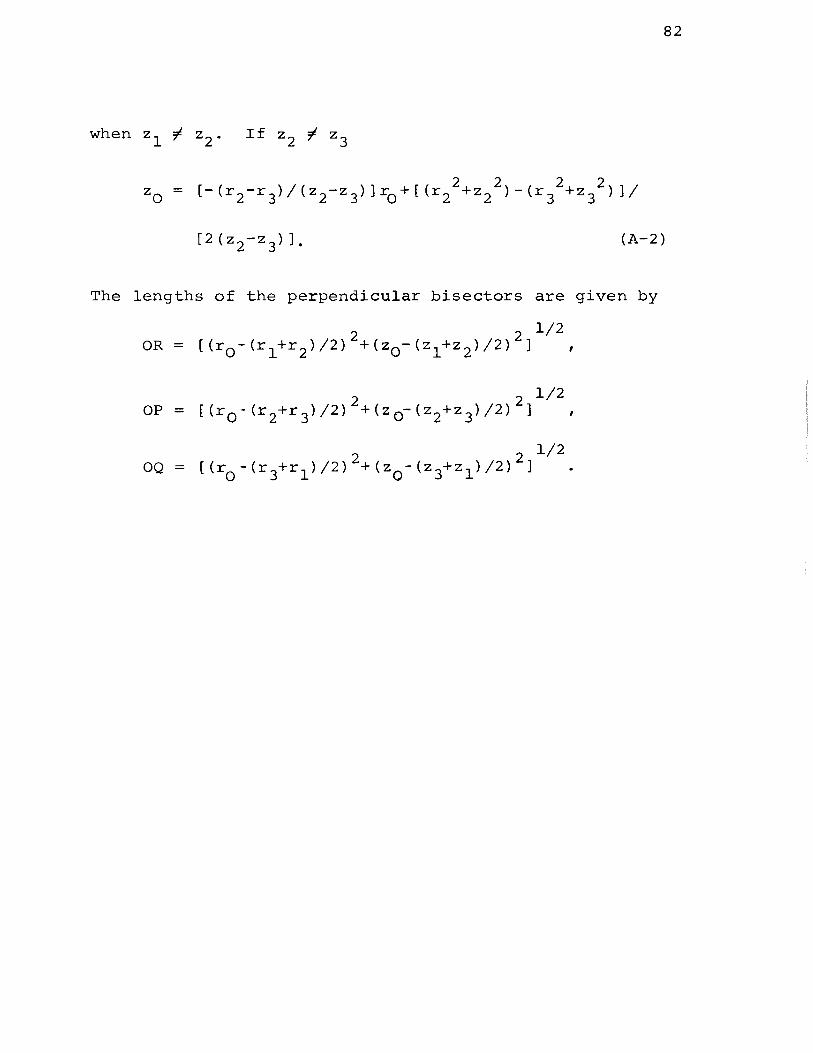
82

(A-2)

The lengths of the perpendicular bisectors are given by

OR

OQ

APPENDIX B

AN ALGEBRAIC APPROACH TO RELATE THE THERMAL CONDUCTANCES OF RECTANGULAR AND TRIANGULAR ELEMENTS

IN CYLINDRICAL COORDINATES

83

Here an algebraic analysis is performed to investi-

gate the possible equivalence of the rectangular (based

on arithmetic mean area) and triangular (case 1 - with

exact area) elements in cylindrical coordinates. The

line of attack resembles Dusinberre's approach in the

two dimensional rectangular coordinates. The results

show that the exact equivalence of the rectangular and

the triangular elements in the cylindrical coordinates

does not exist. The numerical approach in Chapter III

supports this conclusion. However, it is difficult to

eliminate the possibility of equivalence. With a care-

fully chosen definition of thermal conductivity for the

triangular elements, it may be possible to establish the

proposed equivalence.

In Fig.Bl, the rectangular element with section

AXYZ is composed of the triangular elements with sections

ABC, AXB, BYC and CZA. The perpendicular bisectors have

mid-points N, L and M. The angle H made by the side AB

with the assumed direction of heat transfer is arbitrary.

The expressions for the geometric factors and hence for

the thermal conductances for both the rectangular and the

triangular elements will now be found.

z

t Fig.Bl.

z . g c f

v " ·y

/

\ /

I /

\ / kl \ /

/ \

e

L

Q --

-

r. l

....._ h ...... ...... ...... u

d r ro

A Sectional View of the Rectangular and Triangular Elements

84

Q

r

It is expected that the geometric factor SR for the

rectangular element, defined on the basis of arithmetic

mean area, has a greater possibility of yielding the

proposed equivalence than that, defined on the basis of

logarithmic mean area. The expression for SR is

SR = [2n((r.+r )/2)e](r -r.). l 0 0 l

(B-1)

Introducing d = r -r. in Eq. (B-1), the geometric factor 0 l

and the thermal conductance can be written as

85

(B-2)

where k is conductivity. For the triangular elements,

the geometric factors are defined on the basis of mid-

radii of the perpendicular bisectors. The geometric

factors are then

(B-3)

The triangular elements with sections ABC, AXB, BYC

and CZA are completely defined by the parameters r., d, l

e, g and h. Hence all pertinent dimensions and angles

can be expressed in terms of these five independent

parameters. It can be shown from geometry that

which

where

/A= /BOP, /B = /COQ, /C = /AOR, etc.,

leads

COT c = COT B =

COT F =

to the trigonometric relations

OR/ (AB/2) I COT A = OP/(BC/2) I

OQ/(CA/2) I COT D = RU/(AX/2) I

PV/(CY/2) I COT G = QW/(CZ/2),

= r. l

+ OA cos (TI/2 - C+H) I

OA = C/(2 sin C).

(B-4)

(B-5)

(B-6)

(B-7)

86

Eq. (B-6) simplifies to

r 0 = ri+(h/2) (COT H- COT C). (B-8)

The radii of the points R, P and Q are

(B-9)

When Eqs. (B-5), (B-8) and (B-9) are introduced into

Eqs. (B- 3) ' the geometric factors can be expressed as

8A-B = 'IT COT C[r.+d/4+(h/4) (COT H - COT C) ] ' l

8 B-C = 'IT COT A[r.+d/4+g/4+(h/4) (COT H -COT C)], l

8 c-A = 'IT COT B[r.+g/4+(h/4) (COT l

H - COT C) ] ,

8A-X = 'IT COT D [r. +d/2] , 8c-Y = TI COT F[r.+d/2+g/2], l l

8c-z = 'IT COT G[r.+g/2). (B-10) l

The cotangents in the above equations may be expressed

in terms of d, e, g and h by using the trigonometric

relations [1],

COT A COT B + COT B COT C + COT C COT A= 1,

COT Kl COT C + COT C COT E + COT E COT Kl = 1,

COT F COT B + COT B COT D + COT D COT F = 1,

COT G + COT A + COT H = COT G COT A COT H.

(B-10)

Representing the cotangents of the angles by the angles

for simplicity, the Eqs. (B-10) can be rewritten as

(B-11) F•B+B•D+D•F = 1, G+A+H = G A H.

With the relations

D = 1/H, F = l/K1 , (B-12)

the expressions for A, B and C are obtained from Eqs.

(B-11) as

A= (G+H)/(GH-1) I B = (HKl-1)/(H+Kl) I

C = (l-EK1 )/(K1+E).

Using the trigonometric relations

(B-13)

COT D = h/d, COT E = g/e, COT F = (e-h) I (d-g) ,

COT G = e/g, COT H = d/h, COT K = (d-g)/(e-h), 1 (B-14)

the Eqs. (B-13) become

COT (dg+eh)/(de-gh), COT 2 2 A= B = (d +h -dg-eh)/

(de-gh) , (B-15)

COT C = (e 2+g2-dg-eh)/(de-gh).

Inserting the values of the cotangents from Eqs. (B-14)

and (B-15) into Eqs. (B-10), all the geometric factors

are expressed in terms of r., d, e, g and h as 1

= n[(e 2+g 2-dg-eh)/(de-gh)] [r.+d/4+(h/4) 1

((e(d2+h 2 )-h(e2+g 2 ))/(h(de-gh)))],

87

88

SB-C = TI[(dg+eh)/(de-gh)] [ri+d/4+g/4+(h/4)

2 2 2 2 ( ( e ( d + h ) - h ( e +g ) ) I ( h (de -gh) ) ) ] ,

8c-A 2 2 = TI[(d +h -dg-eh)/(de-gh)] [r.+g/4+(h/4)

l

2 2 2 2 ((e(d +h )-h(e +g ))/(h(de-gh)))]

8A-X = TI [h/d] [r.+d/2], l

8c-Y = TI [ (e-h)/(d-g)] [r.+d/2+g/2], l

8c-z = TI [e/g] [r. +g/2]. (B-16) l

The resultant conductance KT of the triangular elements

in the direction of heat transfer can be obtained by the

electrical analogy as

(B-17)

The individual geometric factors, obtained from Eqs.

(B-16) were substituted in Eq. (B-17) to get KT in terms

of ri, d, e, g and h. The expression for KT was then

simplified. This simplification showed that the exact

equivalence did not exist.