Embed Size (px)
Citation preview

MA
STER
THESIS


Technical report, IDE1220
Extracting Maintenance Knowledge from
Vehicle Databases
Master’s Thesis in Information Technology
Magesh Krishnamaraja
School of Information Science, Computer and Electrical Engineering Halmstad University

Abstract
Every vehicle or truck manufacturer maintains databases regarding the service information of their vehicles. In this thesis, two vehicle databases: Vehicle Specification Database and Maintenance Service Database are analyzed and compared. The purpose is to explore the connection between vehicle specification and vehicle maintenance needs. The approach is to use different clustering algorithms(Hierarchical, K-means, Spectral), distance measures (Positive Matching Index and a modified Positive Matching Index), cluster validity measures(Rand Index, Jaccard Index) and data representations(Binary, Frequency) on these databases to determine the important maintenance related specification attributes and their relation to different service problems (e.g. engine, brake, clutch) The clustering results indicate that there is a relation between vehicle specification and vehicle maintenance profiles. Different data mining rules that connect vehicle specification with vehicle maintenance needs are derived from the clustering results.

Table of Contents .................................................................................................................................. .
Chapter 1: Introduction ....................................................................................................................... 1.
1.1 Background Knowledge................................................................................................................. 1.
1.2 Problem Description ...................................................................................................................... 2.
1.3 Thesis Structure ............................................................................................................................. 2.
Chapter 2: Related Work ..................................................................................................................... 3.
Chapter 3: Data ..................................................................................................................................10.
3.1 Database Information .................................................................................................................10.
3.1.1 Global Truck Application (GTA) ...............................................................................................10.
3.2 Vehicle Specification Database (VSD) ........................................................................................11.
3.3 Maintenance Services Database (MSD) .....................................................................................11.
Chapter 4: Method ............................................................................................................................13.
4.1 Overview of Data Mining ............................................................................................................13.
4.2 Overview of Clustering ................................................................................................................13.
4.3 Clustering Algorithms ..................................................................................................................15.
4.3.1 Hierarchical Clustering Algorithm ...........................................................................................15.
4.3.2 K-Means Clustering Algorithm.................................................................................................16.
4.3.3 Spectral Clustering Algorithm ..................................................................................................17.
4.4. Similarity or Distance Measures ................................................................................................19.
4.4.1 History of Similarity measures and their pros and cons ........................................................19.
4.4.2 Theoretical Requirements of Similarity measures .................................................................20.
4.4.3 Motivation for PMI ...................................................................................................................22.
4.4.4 PMI in Vehicle Databases .........................................................................................................22.
4.5 Clustering Validation Indices ......................................................................................................23.
4.6 Cluster Validity .............................................................................................................................25.
4.7 Comparing Clustering Techniques ..............................................................................................26.
4.8Representations used...................................................................................................................26.
4.9 C4.5 algorithm .............................................................................................................................27.
Chapter 5: Results ..............................................................................................................................28.

5.1 Analyzing Vehicle Specification Database .................................................................................28.
5.1.1 Selecting the attributes ............................................................................................................28.
5.1.2 Preprocessing Data...................................................................................................................28.
5.1.3 Finding a more compact representation ................................................................................29.
5.1.3.1Clustering base on 13 GTA attributes ...................................................................................29.
5.1.3.269 GTA+ attributes .................................................................................................................30.
5.1.4 Profiles of the vehicles .............................................................................................................32.
5.2 Maintenance Service Database (MSD) .......................................................................................33.
5.2.1 Parsing of MSD .........................................................................................................................33.
5.2.2 Clustering of Maintenance Data..............................................................................................35.
5.2.3 Grouping of Operations ...........................................................................................................35.
5.2.4 Representation of MSD ............................................................................................................36.
5.3 Finding Outliers ............................................................................................................................37.
5.3.1 Outliers in MSD .........................................................................................................................37.
5.4 Comparing the clustering with 13 or 69 or 425 attributes ....................................................... 39.
5.5 Cluster Validation results on Service Database .........................................................................46.
5.6Binary representation of Data in MSD ........................................................................................49.
5.7 Clustering Matrices between VSD and MSD..............................................................................51.
5.8 Interesting results .......................................................................................................................54.
5.9 Clustering matrix after changes..................................................................................................55.
5.10Data Mining Rules on Vehicles ..................................................................................................60.
5.11PMI and Modified PMI ...............................................................................................................63.
5.12 Comparing results of Clustering Algorithms ............................................................................64.
Chapter 6: Analysis and Discussion ..................................................................................................67.
6.1 Critical attributes and operations for vehicles ..........................................................................67.
6.2 Need for previous knowledge on vehicles .................................................................................67.
Chapter 7: Conclusion .......................................................................................................................68.
Chapter 8: Future Work.....................................................................................................................69.
Chapter 9: References .......................................................................................................................70.

List of Figures ......................................................................................................................................... .
1. Sample Picture of maintenance service database of a vehicle ..................................................12.
2. Diagram for working of Hierarchical Clustering Algorithm.........................................................15.
3. Diagram for working of K-Means Clustering Algorithm ..............................................................17.
4. Diagram for working of Spectral Clustering Algorithm ...............................................................18.
5. Total number of different operations, parts and other codes in MSD ......................................34.
6. Index values when comparing clustering’s of 13 and 69 attributes for VERSION-1 ................40.
7. Rand and Jaccard index values when using random clusterings ...............................................41.
8. Index values when comparing clustering’s of 13 and 425 attributes for VERSION-1 ..............42.
9. Index values when comparing clustering’s of 69 and 425 attributes for VERSION-1 ..............43.
10. Index values when comparing clustering’s of 13 to 69 attributes for VERSION-2 ................44.
11. Index values when comparing clustering’s of 13 to 425 attributes for VERSION-2 ...............44.
12. Index values when comparing clustering’s 69 to 425 attributes for VERSION-2 ....................45.
13. Validity values for Random, Synthetic and Real Data ...............................................................47.
14. Validity values with Mean and SD for 1,2,3,4,5 dataset in MSD ..............................................48.
15. Sample of Frequency representation of MSD ...........................................................................49.
16. Sample of Binary represenation of MSD....................................................................................50.
17. Clustering results using binary and frequency representation ................................................50.
18. Rand Index values for 5 subsets from 2-6 clusters....................................................................54.
19. Rand index values when different operation groups are removed-Part A .............................56.
20. Rand index values when different operation groups are removed-Part B .............................56.
21. Decision Tree for VSD ..................................................................................................................61.
22. Histogram of Service Profiles of VSD for 3 Clusters ..................................................................62.
23. Graph of Service Profiles of VSD for 3 Clusters .........................................................................62.
24. Service Profiles of Vehicles with PMI .........................................................................................63.
25. Service Profiles of Vehicles with Modified PMI .........................................................................64.
26. Comparing algorithms .................................................................................................................65.

List of Tables .......................................................................................................................................... .
1. Description of Vehicle Specification Database ............................................................................10.
2. Example for attributes and their description ..............................................................................11.
3. Changes in PMI calculation attributes .........................................................................................23.
4. Clustering based on number of values of the attributes ............................................................28.
5. GTA attributes and their names ...................................................................................................29.
6.69 important attributes and their names .....................................................................................30.
7. VERSION 1 vehicle profiles with 13 attributes.............................................................................32.
8. VERSION 2 vehicle profiles with 13 attributes.............................................................................32.
9. Example for different operation codes with their description...................................................34.
10. Example for different parts codes with their description ........................................................34.
11. Different operation groups in MSD ............................................................................................35.
12. Number of vehicles with their age .............................................................................................37.
13. Number of vehicles with their Mileage......................................................................................38.
14. Index values when comparing clustering’s of 13 and 69 attributes for VERSION-1 ..............40.
15. Index values when comparing clustering’s of 13 and 425 attributes for VERSION-1 ............41.
16. Index values when comparing clustering’s of 69 and 425 attributes are VERSION-1 ...........42.
17. Index values when comparing clustering’s of 13 to 69 attributes are VERSION-2 ...............43.
18. Index values when comparing clustering’s of 13 to 425 attributes are VERSION-2 ..............44.
19. Index values when comparing clustering’s 69 to 425 attributes are VERSION-2 ...................45.
20. Clustering Matrix when VSD and MSD are clustered into two clusters ..................................52.
21. Clustering Matrix when VSD and MSD are clustered into three clusters ................................52.
22. Clustering Matrix when VSD and MSD are clustered into four clusters ..................................52.
23. Clustering Matrix when VSD and MSD are clustered into five clusters ...................................53.
24. Matrix of Ideal example-1 for interesting results .....................................................................54.
25. Matrix of Ideal example-2 for interesting results .....................................................................54.
26. Clustering Matrix when cluster operations are removed .........................................................57.
27. Clustering Matrix when sensor operations are removed .........................................................58.
28. Clustering Matrix when absorber operations are removed .....................................................59.

29. Data Mining Rules for Vehicles ...................................................................................................62.


Introduction
1
Chapter 1: Introduction
In a fleet of vehicles, maintenance needs can differ from one vehicle to another. It is important to understand the different needs of the vehicles to better serve the problems and improve the performance of the vehicles. Vehicle manufacturers face a challenge with extending the time intervals between maintenance services to reduce service costs, without causing engine problems, with increased downtime, transmission repairs etc. Lyden [1] suggest looking at vehicles’ maintenance service histories as one of the most useful actions to avoid increasing vehicle downtime in these cases, and especially to identify vehicles that are used in the wrong way.
Every OEM (Original Equipment Manufacturer) maintains databases with information about their vehicles. For example, a vehicle service agreements database has information about the service agreements of the vehicles sold; a vehicle specification database has information about the specification attributes of the vehicles when they were built and so on. Maintenance information is collected about the vehicles every time they visit contracted service centers. In the services database, information like time of fault, number of parts changed and number of operations done are stored. This kind of information or databases is underutilized by OEMs. These databases could be utilized as a source for finding new knowledge in order to improve their performance and business decisions. For example, to determine which vehicles that share similar service profile patterns. This can help to serve the maintenance needs of the vehicles better.
Extracting information from these kinds of databases can help the OEM to determine the feasibility of extending a particular vehicle’s service time, effectively spot the defects occurring, determining different maintenance related problems, important vehicle specification attributes related to maintenance and formulate proper service planning to improve the quality of the vehicle components. Useful interpretation of this data can help to save service costs, valuable time of the customer and attain the goodwill of the customer. Even though the existence of useful information in these databases is evident the kind of tools we use to get the required results is equally important. It will be interesting to know whether data mining tools could be used to extract the knowledge from these databases.

Extracting Maintenance Knowledge from Vehicle Databases
2
1.2 Problem Description:
This thesis is done with a goal to:
- Investigate how maintenance needs vary in a large group of similar vehicles; - determine which vehicles that have similar service profile patterns and which
vehicles that do not; - Determine whether there is any correlation between the maintenance history and
the specification of the vehicle; - Determine the important attributes in the vehicles’ specifications and service
operations done in the vehicles and understand their effects from a maintenance perspective;
- Determine what kind of data representations and distance measures that are suitable to use for these databases.
1.3 Thesis Structure:
The thesis is organized as follows: Section 2 presents an overview of related papers; Section 3 describes the relevant OEM databases that have been used; Section 4 presents the method; Section 5 presents the experiments and results with corresponding figures and explanation; Section 6 deals with analysis and discussion; Section 7 draws the conclusions that; Section 8 discusses the future work.

Related Work
3
Chapter 2: Related Work
To investigate the maintenance needs of the vehicles, we are in need of maintenance databases from a large vehicle manufacturer. The data mining techniques we use in this thesis have never before been implemented on the databases we got from the manufacturer. Techniques implemented by previous authors on other databases can give us knowledge on methods, distance measures and tools used. Collecting the references from a manufacturing field where data mining techniques have been used is a good starting point.
Global Competition forces manufacturing enterprises to reduce costs, increase quality and efficiency and to be more flexible, in order to sustain their competitiveness [2]. Data Mining has been used in many fields especially in industrial manufacturing. We review how data mining has been used in the past to improve maintenance operations.
The literature search was done using IEEE databases, Springer link, Google search and references from those IEEE papers. The keywords mostly used to search them were Data mining; truck maintenance; Data mining in maintenance data; data mining in manufacturing; Data mining in automobiles; Data mining techniques; Text Data mining; data mining in warranty claims; Data mining in large vehicle organizations; Data mining in maintenance histories; maintenance problems in trucks etc.
“Data Mining in Manufacturing : A Review” by Harding, Shahbaz, Srinivas and Kusiak [3] gives an overview of data mining applications in manufacturing in the areas of maintenance, control, customer relationship management, decision support systems, fault detection, quality detection and engineering design. The paper also explains the different data mining methods applied previously on these applications for improvement. Their literature work is mainly focused on data mining applications and different case studies in manufacturing. In each of those application sections, they have given a time series and their references to the history of data mining development and implementation.
Especially in maintenance, a key importance should be given to preventive maintenance. This can be achieved by analyzing the databases containing the events of failure of the machines and their respective behavior at the time of failure. The results of this analysis can be used for the design of maintenance management systems. They concluded that there is a significant growth in the number of publications in the manufacturing fields like fault detection, quality improvement and manufacturing and design in recent years, but there are still fields such as customer relationships and shop floor control that have gotten less attention. They also mention that there are few analysis reports in maintenance.
“Data mining in manufacturing: a review based on the kind of knowledge” [4] is another paper by J A Harding et.al that reviews the literature that deals with knowledge discovery and data

Extracting Maintenance Knowledge from Vehicle Databases
4
mining applications in the manufacturing domain. A special attention is given to the type of functions to be performed on data. The data mining functions they include are characterization and description, association, classification, prediction, clustering evolution and analysis. The entire knowledge discovery process is explained with different steps including collecting the target data, data cleaning, preprocessing and transformation, choosing data mining algorithm etc.
For classification in manufacturing, the general techniques used are decision tree induction, Bayesian classification, Bayesian belief networks, neural networks and various hybrid methods are also used. In fault diagnostics, they refer to Skormin et al. [5] where they presented a classification model for the database containing information about monitoring system of flight critical hardware. They used a decision tree based data mining model for accurate assessment of probability of failure of any unit by having their historical data.
In the maintenance category they refer to the paper “Analyzing maintenance data using data mining methods” by Romanowski and Nagi[6] where they implemented decision tree based approach on a scheduled maintenance dataset. They used data mining methods to identify subsystems that are responsible for low equipment availability. From the results, they recommended a preventive maintenance schedule. The sensors data is also analyzed to determine the type of fault occurred to the equipment. They conclude that the data mining results produced using decision tree are easily understandable. In the same paper, for prediction in maintenance data they refer to Sylvain et al.[7] where they used different data mining techniques (detailed overview is presented in later part of this chapter).
In the analysis and discussion after doing several text mining experiments, they determined several features that are commonly used by data mining practitioners. The most important of them are increased use of hybrid algorithms; there is no universally best data mining method for all manufacturing contexts, increased use of combinations of traditional data mining algorithms to get advantages from each technique used. They also provide a correlation and linkage mapping between knowledge area, knowledge mined and techniques used to provide an appropriate choice of techniques for the user. They conclude that hybridization of data mining algorithms may lead to a better solution than existing and traditional algorithms.
From this conclusion we have learned that using different mining algorithms instead of one will help us in producing better results. This also made us aware of combining different traditional mining techniques that are used in the past to get advantage from each technique. We also understood how concept description, classification, clustering, prediction and association are done especially in manufacturing in the past. The mapping diagram gave between knowledge areas, knowledge mined and technique used is clear and understandable. We have learned the

Related Work
5
kind of preprocessing steps, classification models and clustering algorithms are suited on our maintenance service databases.
“Clustering and Classification of Maintenance Logs: using Text Data Mining” by Brett Edwards and Micheal Zatorsky [8] describes the data preparation steps that are needed to transform low quality data into a format suitable for using data mining techniques. The data quality problems that impact the analysis of data are identified in the initial assessment. The problems include long text fields, missing white space between words, inconsistent use of terms and acronyms, repeated words, and concatenated words, misspelling and missing values in many columns. Their case study data is also missing some important columns especially a target column that would differentiate the scheduled maintenance jobs and unscheduled faults. They solved this problem by asking the experts who worked in dam pumped stations to differentiate the scheduled maintenance jobs and unscheduled faults.
After transforming, they mined by calculating term weights and different clustering algorithms are used later on. They determine the different facets or clusters present in maintenance histories (last twelve years of dam pump station). A classifier has been trained to cluster the records into a number of scheduled and unscheduled maintenance problems occurs in different aspects. Their results say that the text clusters produced cannot be clearly classified as scheduled and unscheduled from cluster descriptors. There are some clusters that contain homogenous type of jobs.
The maintenance data that we are going to use contain the same kind of problems. Their case study analysis provided useful information on how to clean the data, format the data, filtering the data, determining text mining stop words and common phrases replacements. This preprocessing step is needed to remove the unwanted data (especially when we are concentrating on maintenance service records) before we are using any clustering techniques. We work also with maintenance related databases. The paper gave us an approach towards how to handle the low quality maintenance records that we learned and used. This paper helped us in solving low quality data problems especially repeated words, misspelling and missing values in many columns that we faced during this thesis.
“Knowledge Extraction from Real-World Logged Truck Data” by Thomas Grubinger and Nicholas Wickstrom [9] proposed how information can be extracted using data mining techniques from logged vehicle database that explains the vehicles’ operation environment. It also explains the extraction of outliers of vehicles that are operated differently from the intended use. The results of the paper showed that logged data holds information that describes the operation environment of vehicles [9].

Extracting Maintenance Knowledge from Vehicle Databases
6
“Maintenance Behaviour based prediction system using Data Mining” by Pedro Bastos, Rui Lopes, Louis Pires, Tiago Pedrosa [2] describes the development of a decentralized predictive maintenance system based on data mining concepts. This proposed system contains the knowledge extraction part, which takes sensor data from the aircraft, analyzes it and gives information on how long the particular component will last. The IDEFO method used consists of three subsystems; namely remote data management and communication (A1), knowledge prediction system (A2) and information synthesis and event generation (A3). A1 is responsible for collecting information about set of parameters from a local perspective to a higher layer. A1 has four sub activities such as data request analysis and specification, data management and selection, knowledge base and definition and decision support formation. The main subsystem that produces knowledge about the equipment is A2 that includes three modules namely data mining processing, pattern behavior generation and proactive failure detection module. The first module outputs are organization knowledge, relations identification, data interpretations and rules. This information will control the next module that will transform the active knowledge base and specification parameters and gives input to the final module of this A2 subsystem.
The behavior matrix in the proactive failure detection module will transform the information into proactive failure notifications. The output will help to advice the maintenance department that is responsible to act in their aircraft parts to avoid the failure. The deviation analysis of equipment behavior using data mining algorithms and pattern recognition algorithms are the basic functionality of this subsystem. Data mining techniques like neural networks, decision trees and regression models are used to predict the failure of the components of the aircraft using data collected from the sensors.
There are various aircraft maintenance related papers “Defect Trend Analysis of F-7P Aircraft through Maintenance History”[10], “Identification of Delay Factors in C-130 Aircraft Overhaul and Finding Solutions through Data Analysis”[11], “Defect Trend Analysis of Airborne fire Control Radar using Maintenance History”[12], “Defect Trend Analysis of Air Traffic Control Radars through Maintenance History”[13] where they have done analysis with their previous maintenance data by determining their defects, component level failures and categorization of defects based on different subsystems on yearly basis. The data mining research has not been done much in these papers.
The paper titled “Data Mining to predict Aircraft Component Replacement” [7] used aircraft sensors data and developed an approach to build models for predicting aircraft component failure. In the meantime, they have addressed several data mining issues. Three years aircraft maintenance data has been used for their analysis. The data they have got contains two major parts: textual descriptions of all aircraft repairs and parametric data acquired through sensors

Related Work
7
during aircraft operation. The four step process they have used consists of data gathering, data labeling, model evaluation and model fusion. The first problem they faced during data gathering process is to select a dataset. They used replacement descriptions from the databases for each component replacement cases (E.g.: date, part removed identifier, textual description of the problem and work performed).
They manually went through the reports and removed operations that were irrelevant to replacement. They then used three different data mining approaches; namely Naive Bayes, decision tree and nearest neighbor. For evaluating methods they split the data into batches; one for validation and the others for training. Their output tables give the part id, approach used, number of times replacement occurs and model’s overall score. Their results demonstrate that experiments with different data mining approaches are required to determine the most suitable approach for a particular problem. In our thesis we have used the same method for evaluating the methods by splitting the data into batches. This has helped us to understand how different clustering algorithms and validity measures are working on our databases. They also conclude that the different approaches tend to make mistakes on different cases.
This paper taught us the basic data mining issues, how to retrieve the information on component replacement, extract key phrases, remove irrelevant component information, labeling each component data, evaluating methods and various data mining approaches. This paper was very relevant for us, because the service records stored in the databases almost matches the fields discussed. (Eg. fields like date of service, part id, comments given by the service engineer). There is also another journal given by same authors where they implemented data mining based models for CF-18 aircraft [14].
“Sequential association rules for forecasting failure patterns of aircrafts in Korean aircraft” by Hong Kyu Han et. al [15] applied sequential association rules to extract the failure patterns. With this they forecast failure sequences of Korean aircrafts according to various combinations of aircrafts types, mission, location and season. They got failure data of four types of aircraft in the year 2004-2005. To determine the sequential association rules they have considered 16 failure modes that occur generally. With these, they have built six scenarios and each scenario is analyzed under four seasons. They set the rule length to be three then they will determine three consecutive failures. They concluded that their analysis provides interesting sequential patterns for each scenario. This paper gives us knowledge on how sequential association rules can be built based on different failure scenarios.
The above referenced papers give an overall idea of data mining applications especially in manufacturing domain. Brett Edwards [8] will help us to understand what kind of data mining issues will arise in maintenance history databases. So the preprocessing steps like getting

Extracting Maintenance Knowledge from Vehicle Databases
8
domain knowledge, cleaning, transforming the data from low quality into format for implementing data mining techniques plays a vital role. The paper [4] explains the types of functions that can be performed on manufacturing data. Especially for maintenance and defect analysis are the mostly used classification models (decision tree), clustering algorithms (hybrid, fuzzy with k-means), prediction techniques (regression tree, decision induction trees, hybrid algorithms), association (association rule among variables) can be learned from their linkage and correlation maps. It aided us to decide on kind of methods that can be used on our maintenance databases.
The paper [9] concludes that logged vehicle data holds the information that describes the operation environment of the vehicles. [15] gives knowledge on how association rules can be used to forecast the failure sequences of aircraft according to the various combinations of aircraft types, mission, location and season. [7] also explains four step process consist of data gathering, data labeling, model evaluation and model fusion will suit to our databases because the maintenance data have same kind of information. For evaluating the methods, they split the whole database into batches which we can use. From our perspective, it is important to decide on suitable methods for our vehicle databases especially when we are dealing with maintenance histories. A combination of traditional data mining algorithms will help us to get advantages from each technique.
Our thesis will helpful if we could give an insight into what kind of information can be drawn from these vehicle databases. The basic domain knowledge that we should have about these vehicles (including the kinds of attributes that plays a vital role in maintenance). The data mining issues that will arise from the databases and how can we solve it and kind of data mining algorithms are suited could be learned. All related papers concentrated or looked into only one database of any particular aircrafts, trucks, pump motors etc. On the contrary this thesis is done using two different databases: Maintenance Services database and Vehicles Specification database. The vehicle specification database describes the attributes of the vehicle, which gives a clear idea of how the vehicle is intended for use. Services database gives a history of services and problems which occurred in that particular vehicle. These results could give some interesting results about the correlation between the services done to the vehicles and their specification.
From reading these papers, we have learned that there are many data mining applications especially in manufacturing field. The basic steps that are needed to transform low quality data into a format suitable for further processing are very important. We have learned what kind of information can be retrieved from the maintenance databases and how can we use it. The knowledge about the important operations about the vehicles is vital so that irrelevant data can be removed. It is important to manually go through the operations done to the vehicles and

Related Work
9
talking with the experts gave a good insight. There are many classification models, clustering algorithms, prediction techniques are available and it is very important to select the right technique that suits to our database. For classification in manufacturing, decision tree induction is used in most of the models for the assessment of probability of unit by having their historical data and the results are easily understandable. For evaluating the techniques we can split the database into many datasets and can validate them. The hybridization of data mining techniques will give us better solutions than using existing and traditional methods. These papers gave us an approach to solve the kind of challenges that we could face during the thesis.

Data
10
Chapter 3: Data
3.1 Database Information
Information about currently maintained databases is provided by the Original Equipment Manufacturer (OEM). We selected three databases in where we expected they contain information relevant for maintenance. They are Vehicle Specification Database (VSD) and Maintenance Service Database (MSD) and Logged Vehicle Database (LVD). The VSD gives details about how the vehicle has been built. MSD contains the detailed explanation of the number of services done to the vehicle. Logged Vehicle Database (LVD), which contains information related to the usage of the vehicle. However, we have used only two databases and unable to investigate LVD due to time constraints.
The motivation for selecting these two databases is that we decided to explore the connection between vehicle specification and vehicle maintenance needs.
We chose to use data that had a low variation among the vehicles, so that we would not see artefacts related to possibly irrelevant factors, like country of operation and different types of vehicles. Data was therefore extracted from the databases with the following limitations:
1. All vehicles are of Type FH12 (Engine Type) Tractors 2. These vehicles are operated in Great Britain 3. The range of operating hours of these vehicles is from 5000 to 15000 hours
The brief description about the database and number of samples obtained from the OEM is shown in Table 1.
Type of Database Vehicle specification Total Number of vehicles considered 4668 Number of Chassis A vehicles 3221 Number of Chassis B vehicles 1447 Type of Vehicles FH12 (Tractor and Rigid) Operating Hours 5000-15000 Place of Operation Great Britain Number of attributes per vehicle 345-375
Table 1: Description of Vehicle Specification Database
3.1.1 Global Truck Application (GTA)
The transport industry is increasingly characterized by specialization and custom(er)ization. This means that the trucks specification and equipment are tailored to suit each particular transport task [16]. The goal is to increase the performance and productivity of the vehicle. Volvo’s Global Truck Application (GTA) defines a number of parameters that specify differences in driving and

Related Work
11
transport conditions for haulage operations all over the world. The typical GTA parameters for FH12 Tractor vehicles that we are going to examine in this thesis are Type of body, Gross Combination Weight, Transport Cycle, Road Condition, Topography, Climate, Altitude, Front Axle Length, Rear Axle Length, Type of Engine, Transmission, Rear Axles, Propeller Shaft, Brakes and Suspension.
3.2 Vehicle Specification Database (VSD)
The Vehicle Specification Database (VSD) describes the attributes of the vehicle (parts of the vehicle) such as Model, Vehicle number, Built week and Engine number. The total number of vehicles that we have is 4668.
The VSD database is provided in HTML file format, which is parsed into excel. The attributes of the vehicle describe how the vehicle has been built, such as the subsystems used, place of manufacture etc.
Examples:
Attribute Description Values ENG-GEN Engine Generation ENG-GEN5,ENG-GEN6 FAL Front Axle Load FAL 16.0,FAL 6.7,FAL 7.1 WTDF Front wheel and tire diameter WTDF22.5 SPEEDDU Dual speed limiter USPEEDDU
Table 2: Example for Attributes and their Description
The following are the problems noticed in this database:
1. Every attribute in the vehicle is given with the description in double quotes of what kind of attribute it is. Some of the attributes lack an explanation code.
2. The same attribute value occurs more than once in the same database entry. However, there were no conflicting attribute values in the same database entry.
3.3 Maintenance Services Database (MSD)
The Maintenance Service Database(MSD) contains information regarding the type of the service done (‘Major A service’ means a major scheduled service has been done), Date of the service, faults found, number of parts changed in the vehicle, mileage of the vehicle, description of the part changed etc. Each and every operation done and parts changed have specific codes attached to them. The information regarding the operations that are performed by the service operator is written in text format.

Extracting Maintenance Knowledge from Vehicle Databases
12
The maintenance database is provided in the form of HTML files. They are parsed into text files. A text file represents a complete history of services done in the vehicle until now. To clearly understand how the database has been maintained and what kind of information has been stored in this database a sample picture is given in Figure 1.
Figure 1: Sample picture of maintenance service database of a vehicle
As shown in Figure 1, the different operation codes are mentioned next to the keyword OPR. They represent the operation done to the vehicle. The parts changed in the vehicle are given using the keyword PRT with their respective codes. The keyword TXT denotes comments by the service operator at the service center.
The following problems were noticed in this database:
1. The codes for some operations and parts changed are missing in some vehicles. For example, OPR will be present but the code for that particular operation is missing.
2. Some of the comments are partially written and are difficult for the reader to understand. Misspellings are frequent (see e.g. REPALCING in the Figure above).
3. In some cases the mileage of the vehicle is missing. 4. The words are redundant and symbols like #,*, <,>, &, are used inside the words and do
not provide any meaning. For example, in one of the vehicles “brake” was mentioned as “>&ake**”.

Method
13
Chapter 4: Method
4.1 Overview of Data Mining
Data mining is the method of analyzing data and extracting different patterns from databases. Data mining can be regarded as an algorithmic process that takes data as input and yields patterns such as classification rules, association rules, or summaries as output [17]. Knowledge Discovery in Databases (KDD) is the traditional method for converting data to knowledge in a usable format. The basic problem addressed by the KDD process is one of mapping low-level data into other forms that might be more compact, more abstract, or more useful [18].
Generally data mining framework has number of tasks that are to be performed in order to effectively extract the information from any database. The important tasks are:
selecting the data, feature extraction, data transformation and clustering of the data
Feature selection includes the attributes that are selected in VSD and operations selected in MSD. Data transformation of these features is done to cluster the vehicles. For most classification and clustering methods it makes a big difference in performance when the data is transformed in an appropriate way before it serves as an input [9]. We have used a similarity measure to determine the similarity between the vehicles. The vectors of vehicles attributes are used as input for the similarity measure.
4.2 Overview of Clustering
Grouping of objects into clusters, based on some common characteristics shared between them is known as Clustering. The aim of clustering is to divide the data objects into clusters so that objects in the same group are similar and objects in different groups are dissimilar to each other. As stated in [19], “Clustering is a common descriptive task where one seeks to identify a finite set of categories or clusters to describe the data”. The selection of the algorithm mainly depends on kind of categorical data, number of features and what the user considers as best suited. We decided to use Hierarchical, K- Means and Spectral, which are explained in the next section.
There exist many clustering algorithms that are used nowadays. The selected algorithms are well known algorithms. Examples of other algorithms that we have not used are Fuzzy C-Means, Expectation-Maximization etc.

Method
14
Several papers [20],[21],[22],[23] compare the performance and suitability of different clustering algorithms.
Ying and George [21] have compared the clustering results of agglomerative and partitional clustering algorithms and evaluated their performance based on seven different global criterion functions. The seven clustering criterion functions used in this paper are classified into four groups: internal, external, hybrid and graph based. Each of the criterion function is defined by an equation. They report that partitional algorithms lead to better clustering results than agglomerative algorithms for each of the criterion function. The clustering results produced by the partitional approach are consistently better than those produced by the agglomerative approach for all the criterion functions [31]. They also determined that hierarchical trees produced by partitional clustering algorithms are always better than results produced by agglomerative algorithms.
Marina and David [22] have done experiments on comparing partitional clustering algorithms (such as Expectation Maximization (EM) and Classification EM) with hierarchical agglomerative algorithm (HAC). They have implemented these three algorithms with a synthetic dataset and a random dataset. They first compared EM and CEM with a larger dataset of 32000 samples with 150 variables. Later, they compare HAC with the better of the two (EM and CEM) since HAC was too slow to run with 32000 samples set. The synthetic data results show that EM is superior to HAC; EM determines twice as many clusters than CEM and HAC.A confusion matrix analysis shows that HAC is unable to distinguish the three largest clusters and its running time is 60 times longer than EM.
In the papers by Abbas [20] and Verma et al. [23], they do several experiments based on the size of the database, number of clusters, type of the datasets etc. In a general conclusion they recommend partitional algorithms for larger datasets. Another conclusion is that K-means works better than Hierarchical clustering with large datasets.
The reasons that we have used Hierarchial clustering algorithm is that we wanted to know how close the vehicle specifications and also maintenance needs of the vehicles. This algorithm helped us to estimate the natural number of clusters from the dendrogram results. It needs only the affinity matrix to give us the output. From the references, we came to conclusion that partitional algorithms works better with larger datasets. We have chosen to use K-means since it is well known and objects in one cluster can be reassigned to another in next iteration and this is not possible in hierarchical clustering. The references also show that K-means works better than Hierarchical clustering when using larger datasets. The algorithm follows a simple procedure and we can manipulate the data by giving various values of k clusters. We have also used Spectral clustering since it uses graph method and each cluster is connected through a

Extracting Maintenance Knowledge from Vehicle Databases
15
path. It calculates eigenvectors which gives the different parititions of objects that are very close to each other. We have chosen to use Hierarchical, K-means and Spectral clustering on these databases.
4.3 Clustering Algorithms
4.3.1 Hierarchical clustering Algorithm
In hierarchical clustering algorithm, two different kinds of approaches are used: agglomerative and divisive. The first step is common for both approaches, which is determining pair-wise distances between the objects using a suitable distance measure. It is followed by constructing a distance matrix of all objects using the distance values.
The divisive method is a top-down approach. The process starts by considering all the objects in the given dataset as one cluster. Now objects that have larger distance in the cluster will split to form new cluster. This process continues iteratively until every object has its own cluster. The agglomerative method works in the opposite direction. Agglomerative method considers each item as a cluster to start with. The process continues by combining the closest pairs of clusters iteratively until the desired K number of clusters obtained. The result can be displayed in the form of a dendrogram (or correspondence tree).
Figure 2: Diagram for working of Hierarchical Clustering Algorithm

Method
16
In Figure 2, an example of clustering of 10 points using hierarchical clustering is shown. The diagram at the left shows the dendrogram. The diagram at the right shows, how the objects are grouped using nested clusters. According to the dendrogram, at the first level of clustering, points (4, 10), (1, 8), (3, 6) are clustered. In the next level (4, 10, 7) and (3, 6, 9) are clustered. In the third step (4,10,7,1,8) are clustered followed by clustering (1,3,4,6,7,8,9,10) points. Later the points 5 and 2 are added in the final two steps of the clustering process. We can notice that at each level it considers the distance between the vehicles and clusters iteratively.
When clustering the points using agglomerative clustering algorithm, at each step the distance between the objects are updated and merged. For example in the above figure, to merge the two clusters (4,10) and (7) we will determine the minimum distance (or shortest distance) between the elements of both the clusters (also known as single linkage clustering algorithm).
The advantage with using a hierarchical clustering algorithm is the dendrogram results where the grouping of data is shown. It can provide clues on the “natural” number of clusters. You do not need to specify the number of clusters. However, estimating the "natural” number from the dendrogram requires that the clustering result is good, which is not always is. The disadvantage of hierarchical clustering algorithm is the time complexity O (N2), which makes it too slow for large datasets.
4.3.2 K-Means Clustering Algorithm
K-Means Clustering Algorithm is a simple and well-known clustering algorithm. This algorithm follows a simple procedure to classify a given data set to a certain number of clusters (K) which is predefined by the user. In the initial stage, an object is selected (randomly or not) for each cluster as centroid. The next step is to take every object in a given dataset and assign it to the nearest centroid. The first cycle of the algorithm is finished, once all the objects in the given dataset are clustered. Later, the centroids are redefined from the objects that are assigned to various clusters. The objects in the clusters are then reassigned to newly obtained centroids on the basis of their respective distance. This process loop continues until there are no more changes to the location of the centroids in clusters (the objects will have minimum distance from their centroids). The algorithm decreases the overall intra-cluster (within-cluster) distance and intra-cluster distance (outside the cluster) since it reallocates the objects iteratively.

Extracting Maintenance Knowledge from Vehicle Databases
17
Figure 3: Diagram for working of K-means Clustering Algorithm [18]
In Figure 3, this algorithm has clustered the objects into two clusters where each cluster is represented by a color. We can notice that in each cluster a centroid is found based on their distances from each other. The centroid is marked using a circle and a cross in the middle. The centroid of cluster is determined by calculating the average distances between the observations inside the cluster. The object that has minimum average distance inside the cluster is known as centroid. The number of clusters (K) is selected by the user.
The advantages of this algorithm are: objects in one cluster can be reassigned to another cluster in next iteration, which is not possible in hierarchical clustering. The algorithm can explore several solutions since the iterations consider all objects in the cluster. The algorithm will converge at some point since the same partition will not occur twice. The time complexity of this algorithm is O (NKI) where, N-number of data points, K- number of clusters and I-number of iterations. The disadvantages of the algorithm are: the initialization of centroids in the first step may lead to problem of local minima, i.e. it will converge to the globally best solution. A good selection of initial points will improve the quality of clusters. The right selection of K (number of clusters) is really important to reach good results. The motivations for selecting this algorithm are its simple, scalable efficient and easy to implement.
In the time complexity of K-means, since K and I are usually much less than N, so K-means can be used to cluster larger datasets. While in Hierarchical clustering, the time complexity is O (N2), this high cost limits their application in large datasets.
4.3.3 Spectral Clustering Algorithm

Method
18
In recent years, spectral clustering has become one of the most popular modern clustering algorithms [24]. If ‘N’ objects are given, we construct a complete graph, where two objects are connected by an edge if two objects are similar. The objects are clustered, even though the objects do not form complete sub graphs because it is sufficient that each cluster is connected through a path. The first step is to determine an affinity matrix which gives the pair-wise distances between all the samples in the dataset. This step is same as Hierarchical clustering algorithm, but Spectral clustering uses this affinity matrix (or Laplacian matrix), to calculate the eigenvalues and eigenvectors to cluster the objects. By calculating the eigenvectors, the different partitions of objects (or vehicles in our case) that are same (and very close objects) can be determined and clustered. Now, we are interested in matrix of U, where columns of eigenvectors are determined. Later we use K-means clustering algorithm to cluster original data point in the given dataset into predefined K number of clusters by taking matrix U as input.
Figure 4: Flowchart Diagram for working of Spectral Clustering Algorithm

Extracting Maintenance Knowledge from Vehicle Databases
19
Figure 4 shows the flowchart for working of spectral clustering algorithms. It explains how the algorithm is implemented.
We have used different toolboxes in Matlab where these clustering algorithms have been implemented already. To implement Hierarchical clustering algorithm functions like pdist (distance between the vehicles), linkage should be used and these are present in the ‘Clusterdata’ toolbox. The ‘stats’ toolbox is used for k-means. We have also experimented statistics toolbox for implementing K-means. One more way is to use standard keyword of ‘kmeans’ by giving the matrix of object distances with the number of clusters (n). For spectral clustering, we have calculated affinity matrix as same as hierarchical clustering and we calculate Laplacian matrix by using a formulae. Later we use that matrix to calculate the eigenvalues and eigenvectors. From those eigenvectors we used K-means to cluster the original data point in the dataset into predefined number of k clusters.
4.4 Similarity or Distance measures
The Distance or Similarity Measure plays a key role in clustering. All clustering algorithms group objects that are “close” together and it is important to measure closeness in an appropriate way. Appropriate distance measures lead to more interesting results.
The vehicles are represented as lists of attributes, both in the case of VSD and MSD, and we must therefore use a distance measure that is suitable for this.
4.4.1 History of Similarity Measures and their Pros and Cons
The vehicles are represented as lists. These lists can be very long and lists from two vehicles will most likely not contain the same number of elements. The list from one vehicle is not likely a subset/superset of the list from another vehicle.
The parameters needed to find the association or similarity between the two lists (we call them V1 and V2) of attributes is
a = number of common entries between the lists
b = number of elements present in V1 which are absent in V2
c = number of elements present in V2 which are absent in V1
d = number of elements absent in both of the lists
The inclusion and exclusion of variable d is discussed by authors like Sokal and Sneath [25] and Goodman and Kruskal [26]. According to the Sokal and Sneath [25] the negative matches is not

Method
20
necessarily needed for determining the similarity between the objects (or lists in our case). The negative matches can be very large in both the lists.
The Sokal& Michener, the Roger & Tanimoto, the Faith, The Ochaiai II, the Cole, the Gower, Pearson I, and the Stiles are some of the similarity measures that use negative matches (d) in their measures. The Jaccard, the Tanimoto, the Dice & Sorenson, the Kulczynski I, the Ochiai I, the Mountford, the Sorgenfrei, and the Simpson are similarity measures that exclude the negative matches (d) in their measures [27].
4.4.2 Theoretical Requirements of Similarity Measures
According to Tullos, there are eight different requirements that a similarity measure has to fulfill [28]. The requirements are given below and they explain how the measures mentioned in the previous section differ from Tullos’ Tripartite Similarity Index (TSI).
1. A similarity index shall be sensitive to the relative size of the two lists to be compared; and great difference in size shall be interpreted to reduce the value of the similarity index.
2. A similarity index shall be sensitive to the size of the sublist shared by a pair of lists; and an increase in difference in size between the smaller of the two lists and sublists of common entries shall be interpreted to reduce the value of the similarity index.
3. A similarity index shall be sensitive to the percentage of entries in the larger list that are in common between the lists and to the percentage of entries in the smaller list that are in common between the two lists and shall increase as these two percentages increases.
4. A similarity index shall yield values having fixed upper and lower bounds. 5. A similarity shall have the property that when two lists are identical, the similarity index
for the two lists shall be equal to the upper bound of the index. 6. A similarity index shall have the property that when two lists have no entries in
common, the similarity index for the lists shall be equal to the lower bound. 7. Distribution of values of the similarity index between zero and one shall be such that (i)
if the size of two input lists is fixed, then the output shall vary roughly directly as the number of entries shared between the lists; and (ii) if the smaller list is a subset of the larger list, then the value of the similarity index shall vary roughly inversely as the size of the larger list.
8. A similarity index program shall check its input data to verify that the following relationships hold: a + b>0 and a +c >0.
The first requirement is explained in more detail below

Extracting Maintenance Knowledge from Vehicle Databases
21
A similarity index shall be sensitive to the relative size of the two lists to be compared and great difference in size shall be interpreted to reduce the value of the similarity index [28].
This requirement is not fulfilled by most of the similarity measures because of “aliasing” (formulae giving the same value for different data inputs). For example:
Jaccard coefficient =
Since the values of b and c are added, the same sum can be produced by many different sizes of lists. Consider (a,b,c) = (5,6,6) same size of lists and (a,b,c) = (5,2,10) different size of lists. When you calculate the coefficient value, both of them gives 0.29 even when there is a large difference in the size of the lists. So, the Jaccard coefficient does not fulfill the above requirement.
The same problem occurs in many other similarity measures, some are given below
Dice coefficient = ( )
Sokal and Sneath Coefficient =
First Kulczynski Coefficient = and so on.
Tullos suggested a similarity measure for lists that met all the above similarity theoretical requirements [28]. He introduced three cost functions (U, S, R) and the Tripartite Similarity Index(TSI) =√푈 ∗ 푆 ∗ 푅.
푈 = log(1 + ( , )
( , ))
푙표푔2
U acts as a penalty function and gives value one when two lists being compared are same in size.
푆 = 1
( ( , ))
R is designed to penalize the index value based on the number of elements between the lists are same. R takes the value one when two lists that are compared are identical.

Method
22
푅 = log 1 + . log(1 + )
(log 2)
If the lists are same sized then reward function R is calculated.
4.4.3 Motivation for PMI
The paper [29] compared the three common similarity measures Jaccard, Dice and Simple Matching coefficients with TSI using medical data from neurophysiology research. Their results showed that the Dice coefficient is the same as that of Tripartite T overall and that TSI has limitations in medical applications due to the reverse function U in TSI [29]. The U function correctly penalizes the unbalanced size of input lists, but turns into a reward function rather than being balanced when the size of the lists are equal [30].
Santos and Deutsch therefore introduced the Positive Matching Index (PMI) [30], which fulfills all the eight requirements of similarity measures listed by Tullos [3] but without the drawbacks of TSI.
The PMI shows improved performance in medical applications when compared to TSI and other coefficients. The equation for PMI is given below
If b = c then PMI =
If b ≠c then PMI = | |
ln( ( , )( , )
)
When b ≠ c, the two different sizes of lists b and c are calculated w.r.t a. Even a small change in the size of the lists will affect the coefficient value.
4.4.4 PMI calculation in Vehicle Databases
The PMI counts matches and non-matches between two lists. In the case of the VSD, however, the concept of a match is not crisp. For some attributes there is an ordering between the values. One example is PLM (Propeller Main Shaft Length), which has about 50 values varying from 825mm to 2225mm. Obviously two values that only differ by 100 mm denote two vehicles that are much more similar than vehicles with values that differ by 1000 mm. We therefore chose to modify the PMI into a “fuzzy” PMI, which allows a gradual match and not just a binary match.
We have manually given fuzzy conditions to determine the distance between the vehicles. We have given a window for the attribute values. So the vehicles with slight change in the values of the same attribute will be considered as similar vehicles. For example, consider two vehicles

Extracting Maintenance Knowledge from Vehicle Databases
23
having same 13 GTA attributes except PLM (PLM0225 and PLM0325), PMI will consider them as binary match in terms of their distance even though their PLM values are very close. In terms of PMI parameters (a, b) will be (12, 1) and here b = c since the vehicles have the same number of attributes.
In our modified PMI (fuzzy PMI), we have considered the values difference from 0-100 in PLM as gradual match. In modified PMI parameters a and b will have 12.9 and 0.1 respectively. We have implemented this modified PMI in VSD and the results have shown a considerable change in clustering results. The modified PMI results are discussed at the end of this chapter.
Table 3 shows the GTA attributes to which we have made changes in their distance calculation of PMI.
Attributes Scale Similarity value GCW(Gross Combination Weight)
0-5 tonnes 5-10 tonnes >10 tonnes
1 0.5 0
FAL(Front Axle Load) 0-0.5 0.5 -1 >1
1 0.5 0
RAL(Rear Axle Load) 0-2.5 2.5-5 >5
1 0.5 0
PLM(Propeller shaft) >0-100 100-200 200-300 300-400 400-500 >500
0.9 0.7 0.5 0.3 0.1 0
Table 3: Changes in PMI calculation Attributes
4.5 Comparing clusterings
We do several experiments where we try different vehicle representations (e.g. number of attributes) or with different data subsets. These experiments are done to test how stable the results are or to see if more compact representations can be used. In order to do this we need measures of cluster structure similarity, i.e how similar two clustering are. This can be done by using cluster similarity indices. Generally databases have different features and functionalities. There are different clustering algorithms that we can use to partition or cluster the data. But it
Method
24
is important to compare and validate the clusters given by the two partitions of same set of data.
The external evaluation of clustering is the process of evaluating the closeness between one clustering structures to another. In recent years, Meila [31,32] has done research on criterions for comparing two partitions or clusterings.. In Meila’s work related to comparing clusterings, the clusterings are viewed as elements of lattice which is the natural algebraic structure for the partitions of a set. In [31], an axiomatic study of several distance measures is presented along with the discussion on some desirable properties of distance between the clusterings.
In [32], Meila discusses about two different criterias that have been previously used. They are: comparing clusterings by counting pairs and comparing clusterings by set matching. In the first criteria that are based on counting pairs indices like Jaccard, Rand, Fowlkes and Mallows are discussed. The second criteria are based on set cardinality. Further, Meila proposed a new criterion called Variation of information that does not fall in any of the above two categories. This criterion measures the amount of information gained in changing from a clustering C1 to clustering C2. Variation of information is based on the relationship between a point and its cluster in each of the two clusterings that are compared. This tells us that with respect to the criteria based on counting pairs it’s neither a direct advantage nor a disadvantage. The papers other than Meila to compare clusterings are given in [33][34][35][36][37]. From these different criterions we have opted to use “comparing clusterings by counting pairs” instead of Variation of information.
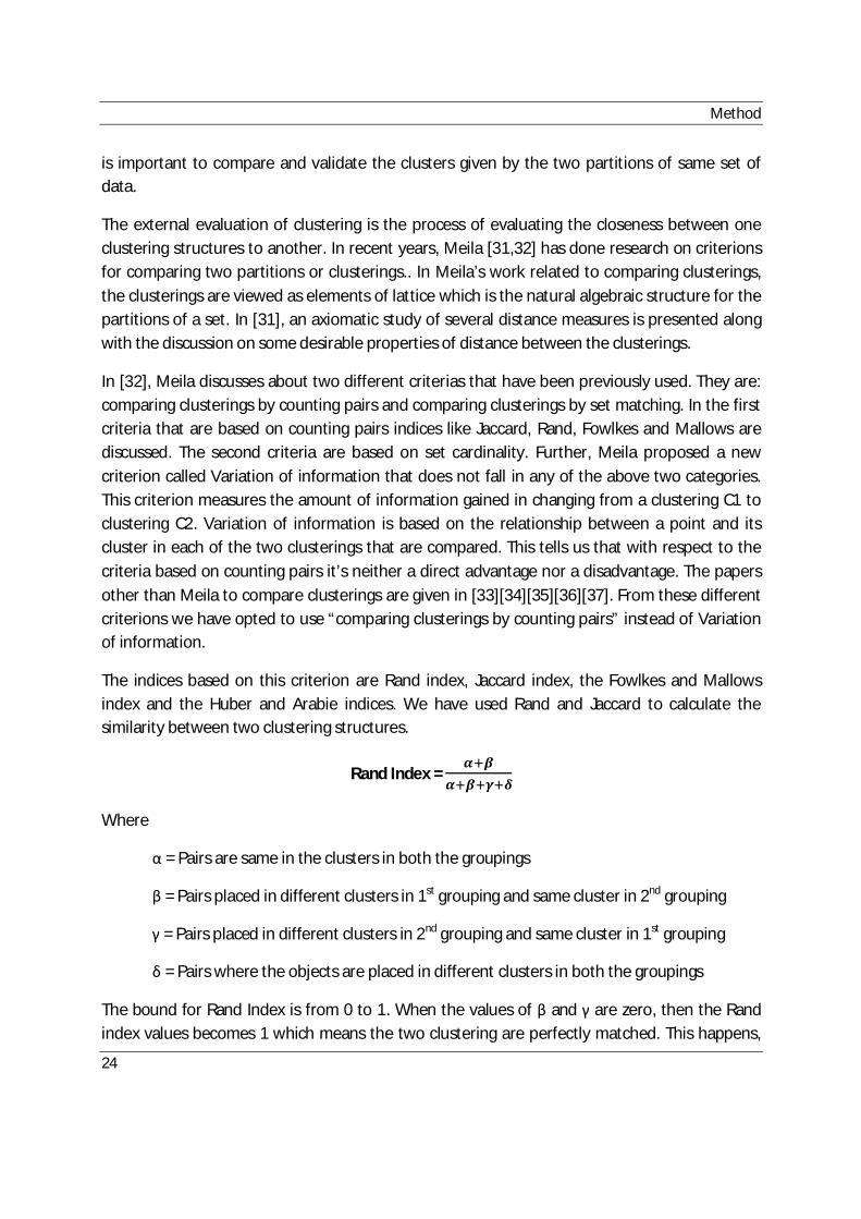
The indices based on this criterion are Rand index, Jaccard index, the Fowlkes and Mallows index and the Huber and Arabie indices. We have used Rand and Jaccard to calculate the similarity between two clustering structures.
Rand Index = 휶 휷
휶 휷 휸 휹
Where
α = Pairs are same in the clusters in both the groupings
β = Pairs placed in different clusters in 1st grouping and same cluster in 2nd grouping
γ = Pairs placed in different clusters in 2nd grouping and same cluster in 1st grouping
δ = Pairs where the objects are placed in different clusters in both the groupings
The bound for Rand Index is from 0 to 1. When the values of β and γ are zero, then the Rand index values becomes 1 which means the two clustering are perfectly matched. This happens,

Extracting Maintenance Knowledge from Vehicle Databases
25
e.g., when the number of clusters is 1. However, when the number of clusters is large, then the probability for objects to end up in different clusters increases (i.e. d increases). Thus, the Rand index should approach 1 when the number of clusters grows. The Rand index should therefore be high for low number of clusters and large numbers of clusters (and lower in between).
The value of δ is the difference between Jaccard and Rand index. We also compute the Jaccard index in order to investigate the change in the index value when we remove the parameter δ.
Jaccard Index =휶
휶 휷 휸
The Jaccard index is also high (equal to 1) when the number of clusters is 1. The probability for two objects to end up in the same cluster in two clusterings decreases with number of clusters. The Jaccard index should therefore decrease with growing number of clusters.
4.6 Cluster Validity
The previous section introduced indices to compare the two different attribute groupings of the same dataset. However, it is also important to determine what the “natural” number of clusters is, i.e. what value K should have. The “cluster validity measure” is used to find the natural number of clusters (k) for a dataset. This measure relates the average distances between the objects inside the clusters (intra cluster distance) to the average distances outside the clusters (inter cluster distance).
Cluster validity = Intra cluster distance/Inter cluster distance
The equations for both distances are given below
Intraclusterdistance = 1푁 ||푋 − 푍 ||
£
.
Interclusterdistance = min( 푍 − 푍 )
The cluster center is the point with minimum distance to all the objects in the cluster (if we use one of the objects as center then it will be the distance to all the other objects in the cluster). The cluster center is denoted by Zi (or Zj) in the equations above. With access to the pairwise distances we can determine the cluster center object for each cluster by taking one object at a time and calculate the summed distance to the other objects in the cluster. The object that has the lowest summed distance will be the cluster center object. The intra cluster distance is the minimum summed distance in the cluster divided by number of objects in the cluster, i.e. the average distance between the cluster center and the objects. The inter cluster distance is the
Method
26
average distances between all pairs of clusters where distance between two clusters is defined as distance between their cluster centers.
If the validity value is close to 0, then vehicles are closely clustered, in other words with “the right” (or a good) number of clusters. The “cluster validity” is also known as the Davies-Bouldin Validity Index [38].
In our databases, inter cluster distance is calculated by determining the average distance between the cluster centers of all pairs of clusters. Cluster center is calculated by taking the average distance of the vehicles inside the clusters and selecting the vehicle which gives less distance to all the objects. Intra cluster distance is determined by calculating the average distance between cluster center and all vehicles in the clusters.
4.7 Comparing Clustering Techniques
We have used three clustering algorithms: Hierarchical Clustering; K-means; and Spectral clustering. We have examined and compared these algorithms on both VSD and MSD databases. The motivation for this comparison is to examine how the algorithms works with the distance measures we use. The results for the comparison are presented in next chapter 5.
4.8 Representations Used
In VSD, we have a total of 425 individual attributes where many attributes have more than 10 values. There are attributes that have only one value. There are many attributes that we deemed not be important from a maintenance point of view. The Global Truck Application (GTA) booklet, which is provided by the Volvo organization, is used to select the attributes. The booklet contains specification attributes that provide the basis for an organization to build a vehicle. It briefly explains the various attributes or parameters that are to be considered by the customer based on road condition in his area, climate, topography, etc. Using this booklet we have selected 13 GTA attributes. We suspected that some more attributes could be important attributes so added them to GTA and reached 69 GTA+ attributes. Thus we end up with three possible representations for the VSD: GTA (13 attributes), GTA+ (69 attributes) and the full 425 attributes.
In MSD, we have different operations that are done to the vehicles (See Section 5.2). Once we have selected the operations to be used, we have represented the MSD in two ways: binary and frequency. Binary representation of data is done by taking presence and absence of operation into consideration. We have also experimented with frequency representation of data by taking the number of times a particular operation has been done to the vehicle.

Extracting Maintenance Knowledge from Vehicle Databases
27
In the method of data analysis, the binary form deserves a special place [39]. The typical examples for binary representation of data are document clustering and market basket data. Each and every document (vehicle in our case) is represented as a vector of presence and absence of the word or term (in our case maintenance operations).
The frequency representation of data gives the number of times an operation occurs in the dataset. The binary representation of data gives the presence and absence of an operation in the dataset. In our analysis, if an operation has been done at least once then we will consider that vehicle in the particular operation category. So we have chosen to use binary representation of data since it gives only presence and absence of data. The results for different representations of data for our given databases are discussed in Chapter 5.
4.9 C4.5 algorithm
C4.5 is an algorithm developed by Ross Quilan [40] to generate a decision tree and it is an extension his previous version ID3. The decision trees produced by the C4.5 algorithm are used for classification. This algorithm builds the decision trees with the aid of sample set using information entropy. The sample set will already be classified samples with each sample has a vector with their respective attributes. We also have the information of which class each sample belongs. With starting from one node, the algorithm selects one attribute at a time and calculates its respective entropy. The attribute with the highest entropy will be selected as leaf node and the data sub listed based on that decision tree.

Results
28
Chapter 5: Results
5.1 Analyzing Vehicle Specification Database
5.1.1 Selecting the Attributes
Feature selection is a vital step in data mining. The extraction of attributes from vehicles is performed and arranged in Excel. Each vehicle consists of attributes ranging from 345-375. Each attribute of the vehicle consists of one or more values to it. For instance, Type of Road is an attribute that has two values: Rough and Smooth. There are 425 attributes that are present in all vehicles. Considering all the attributes for clustering will be a difficult task and noisy. Some attributes like Radio and Rear View Mirrors in a vehicle have little effect on the maintenance needs of the vehicle. The motivation for reducing the number of attributes is to simplify the problem so that it will be easier to define the different data mining rules for these two databases.
5.1.2 Preprocessing Data
The attributes of the vehicles have been grouped in two different ways.
1. Clustered based on the number of values of each attributes. For example, attributes with only one value and attributes with more than one values etc.. The types are explained in Table 3.
2. Clustered based on conditional probabilities
1. Clustered based on Number of Values
The total number of attributes in our VSD data set is 425. Some attributes have values for all vehicles (which we denote as “complete”). Some attribute values will only be present in some vehicles (which we denote as “incomplete”). There are many attributes that have only one value. There are attributes that have more than one value. Table 4 shows the different attribute descriptions.
Type Description of the clusters Complete or Incomplete 1 Attributes with only one value Complete (attribute is present in all vehicles) 2 Attributes with only one value Incomplete (attribute is present in some
vehicles and absent) 3 Attributes with more than one value Complete (attribute is present in all vehicles) 4 Attributes with more than one value Incomplete (attribute is present in some
vehicles) Table 4: Clustering based on number of values of the attributes

Results
29
This information helps to understand the kind of attributes present in this database. For example, attributes that are constant, attributes that have more values and attributes that have no values etc.. By this, we can even reduce (by removing the attributes that are constant in all vehicles) the number of attributes that need to be considered.
2. Clustered based on conditional probabilities
It is important to determine redundancies and relationships between attributes in order to remove attributes that are redundant. This can be done by calculating the conditional probabilities between the attributes. The results showed that most of the attributes that differ in the vehicles are based on the difference between VERSION-1 and VERSION-2 vehicles. We therefore divided the VSD data set into two subsets: VERSION-1 and VERSION-2 vehicles.
5.1.3 Finding a more compact Representation
5.1.3.1 Clustering based on 13 GTA attributes
The attributes were grouped into 13 GTA (Global Truck Application) attributes, as described in the GTA booklet. These GTA attributes were selected based on vehicle utilization and operation environment. These attributes should reflect how the particular vehicle was intended to be used, since the GTA booklet is an aid for buyers.
There is a total of 425 individual attributes (that are present in all vehicles). Each attribute has a set of possible values, from a minimum of 1 to a maximum of around 50. Out of these attributes 13 GTA attributes are selected manually. The attributes are listed in Table 5.
Name of the Attribute 1. Type of vehicle 2. Road condition (rough or smooth) 3. Gross combination weight 4. Front axle load 5. Rear axle load 6. Engine Type 7. Transmission 8. Propeller Shaft Dimension 9. First Propeller Shaft Length 10. Second Propeller Shaft Length 11. Main Propeller Shaft length 12. Brake 13. Rear axle bogie type
Table 5: The 13 GTA Attributes and their names

Extracting Maintenance Knowledge from Vehicle Databases
30
The attributes given in Table 5 are used to cluster the vehicles. The modified Positive Matching Index (m-PMI) is used to find the distance between the vehicles. The resulting distance matrices used as input to the clustering algorithms.
5.1.3.2 69 GTA+ Attributes
The 13 GTA attributes are complemented with more attributes that we suspected would be important from a maintenance perspective. This lead to a total of 69manually selected attributes. They are given with their names in Table 6.
Name of the Attribute 1. Wheels 2. Type of vehicle 3. Version 4. Road condition (rough and smooth) 5. Gross combination weight 6. Front axle load 7. Rear axle load 8. Wheel base 9. Engine type 10. Engine torque range 11. Secondary fuel filter info 12. Fuel tank filter 13. Primary fuel filter 14. Exhaust direction 15. Engine emission level 16. Turbo compound 17. Air cleaner 18. Air intake 19. ATB Cooling capacity 20. Radiator size 21. Engine protection 22. Battery protection 23. Load indicator for the electrically controlled suspension 24. Clutch info 25. More clutch info 26. Transmission software 27. Transmission 28. Gear shifting 29. Propeller Shaft 30. First propeller shaft length 31. Second propeller shaft length

Results
31
32. Main propeller shaft length 33. Rear axle specifications 34. Rear axle ratio 35. Power take out engine rear 36. Power take out engine Front 37. Power take out engine side 38. Transmission cooler 39. Brake System 40. Air dryer 41. Air compressor, more 42. Air tank material 43. Air tank capacity 44. Auxiliary air tank 45. Auxiliary air tank 46. Air tank with rubber rings 47. EBS (electrical brake system) package 48. Front axle load 49. Number of front axles 50. Rear axle bogie type 51. Rear axle configuration 52. Axle load transfer 53. Rear suspension height 54. Tag axle 55. Load on trailing axle 56. Rear axle load limiter 57. Front under run protection system 58. Front suspension system 59. Rear suspension system 60. Rear shock absorber 61. Front axle load limiter 62. Leveling device 63. Tire Pressure Monitoring 64. Cab Suspension 65. Front Cab Suspension 66. Engine Block Heater 67. Hydraulic Pump Gearbox mounted 68. Central Lubrication 69. Factory
Table 6: 69 important attributes and their names

Extracting Maintenance Knowledge from Vehicle Databases
32
5.1.4 Profiles of the vehicles
The vehicles are analyzed based on 13 attributes for finding the number of vehicles which share the same GTA specification profiles. The vehicles are divided into VERSION1 and VERSION2 vehicles. Tables 7 and Table 8 show the number of vehicles that share the same profiles. These profiles give an overall idea of how the vehicles’ attributes differ and number of vehicles that have these kinds of profiles in the total dataset. The description of the attributes is shown in Table 5.
Number of attributes used: 13 (GTA attributes)
Number of VERSION 1 vehicles: 361
Profiles
TYPE OF PROFILE NUMBER OF VEHICLES PROPS-M,D12C420,VT2014,BRAKE-ZV,GCW44.0,PLM0825,UPLF,FAL7.1,UPLS,RAPD-A6,RAL19,RC-SMOOTH,TRACTOR
65
VT2014,GCW52.0,BRAKE-ZV,PLM0850,UPLF,FAL7.1,D12C380,UPLS,RAPD-A6,RAL19,PROPS-L,RC-SMOOTH,TRACTOR
24
Table 7: VERSION 1 Vehicle Profiles with 13 attributes
The above profiles have attributes BRAKE-ZV (Disk brake),RC-SMOOTH (Smooth road condition),RAPD-A6 (Rear axle bogie type-Air Suspension),UPLS (Second Propeller Shaft Length),UPLF (First Propeller Shaft Length),TRACTOR (Type of vehicle), FAL7.1 (Front Axle Load),RAL19 (Rear Axle Load),VT2014 (Transmission) in common.
Number of VERSION 2 vehicles: 4307
Profiles
TYPE OF PROFILE NUMBER OF VEHICLES PROPS-M,D12D460,BRAKE-DV,GCW44.0,VT2412B,UPLF,FAL7.1,PLM1000,UPLS, RAPD-A6,RAL19,RC-SMOOTH,TRACTOR
701
PROPS-M,D12D420,BRAKE-DV,PLM0850,GCW44.0,UPLF,FAL7.1,UPLS,RAPD-A6,RAL19,RC-SMOOTH,VT2214B,TRACTOR
288
PROPS-M,D12D460,VT2514B,BRAKE-DV,PLM0850,GCW44.0,UPLF,FAL7.1,UPLS,RAPD-A6,RAL19,RC-SMOOTH,TRACTOR
501

Results
33
PROPS-M,D12D460,BRAKE-DV,GCW44.0,VT2412B,PLM1200,UPLF,FAL7.1,UPLS,RAPD-A6,RAL19,RC-SMOOTH,TRACTOR
244
PROPS-M,D12D460,VT2514B,BRAKE-DV,GCW44.0,UPLF,FAL7.1,PLM1050,UPLS,RAPD-A6,RAL19,RC-SMOOTH,TRACTOR
377
PROPS-M,D12D420,BRAKE-DV,GCW44.0,UPLF,FAL7.1,PLM1050,UPLS,RAPD-A6,RAL19,RC-SMOOTH,VT2214B,TRACTOR
100
PROPS-M,D12D420,BRAKE-DV,GCW44.0,VT2412B,UPLF,FAL7.1,PLM1000,UPLS,RAPD-A6,RAL19,RC-SMOOTH,TRACTOR
362
Table 8: VERSION 2 Vehicle Profiles with 13 attributes
The above profiles have attributes PROPS-M (Propeller Shaft Dimension- Single Joint),BRAKE-DV (Disk brake),GCW44.0 (Gross Combination Weight),TRACTOR (Type of vehicle),RC-SMOOTH (Smooth road condition),RAL19 (Rear Axle Load),RAPD-A6 (Rear axle bogie type-Air Suspension),UPLS (Second Propeller Shaft Length),UPLF (First Propeller Shaft Length),FAL7.1 (Front Axle Load) in common.
Once we determined the attributes’ values changes mostly by the version (V1 and V2), we were eager to know the typical vehicle types (or profiles) and the attributes that are present in both these versions. So we have extracted the 13 GTA attributes of typical vehicle types with their respective frequency to know the percentage of vehicles that have the same configuration (within V1 and V2). Tables 7 and 8 show the typical vehicle specifications of 13 GTA and how many vehicles that have this profile within V1 and V2.
5.2 Maintenance Service Database (MSD)
5.2.1 Parsing of the MSD
Maintenance database information is extracted by collecting all the possible information such as the operations done, parts changed till now, comments given by the service operator, Date of service and Mileage for each vehicle. An operation describes the type of repair that has been done on the vehicle.
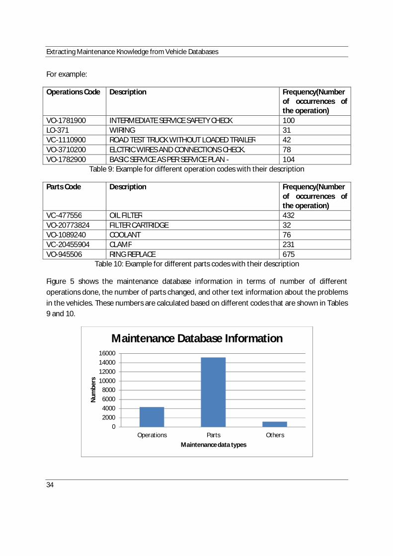
Extracting Maintenance Knowledge from Vehicle Databases
34
For example:
Operations Code Description Frequency(Number of occurrences of the operation)
VO-1781900 INTERMEDIATE SERVICE SAFETY CHECK 100 LO-371 WIRING 31 VO-1110900 ROAD TEST TRUCK WITHOUT LOADED TRAILER 42 VO-3710200 ELCTRIC WIRES AND CONNECTIONS CHECK. 78 VO-1782900 BASIC SERVICE AS PER SERVICE PLAN - 104
Table 9: Example for different operation codes with their description
Parts Code Description Frequency(Number of occurrences of the operation)
VO-477556 OIL FILTER 432 VO-20773824 FILTER CARTRIDGE 32 VO-1089240 COOLANT 76 VO-20455904 CLAMP 231 VO-945506 RING REPLACE 675
Table 10: Example for different parts codes with their description
Figure 5 shows the maintenance database information in terms of number of different operations done, the number of parts changed, and other text information about the problems in the vehicles. These numbers are calculated based on different codes that are shown in Tables 9 and 10.
02000400060008000
10000120001400016000
Operations Parts Others
Num
bers
Maintenance data types
Maintenance Database Information

Results
35
Figure 5: Total Number of different Operations, Parts, Others codes in Maintenance database
5.2.2 Clustering of Maintenance data
Three clustering algorithms (Spectral, K-means and Single Linkage) are used to cluster the vehicles in the whole dataset. Later the data was divided into five subsets and then clustered using the same procedure. This was done to determine the consistency in the results.
5.2.3 Grouping of Operations
The results show that operations play a vital role and give an idea on the kind of repair or fault that happened to the vehicle. There are a total of 4360 different operations present in all the given vehicles. All the operations are not important from a maintenance point of view. Operations related to radio, tires, and wiring will have little effect on maintenance. We therefore manually selected subgroups of important operations (operations that are deemed important from a maintenance perspective).The groups are explained in Table 11.
Group id Operation Group Individual Operations 1 Engine
D12C Engines ECU Fault tracing Engine brake function check Engine Oil Leak Steam Clear Engine Engine Fan Engine Noise Engine Misfiring Engine Encapsulation Replace Engine Engine Starting Difficulties
2 Clutch Clutch Replace Clutch System Bleed
3 Brakes N/S/F Brake Cylinder replace Front Axle brake linings replace Replace NSR Brake chamber Brake Pads
4 Gearbox Gearbox remove Gearbox replace
5 V-Rod Remove V-Rod drive axle 6 Oil Engine Oil
Gear Box Oil VDS3 Motor Oil

Extracting Maintenance Knowledge from Vehicle Databases
36
7 Sensor Rep. Air Suspension level Sensor NSR Level Sensor Replace Sensor Air Pressure Sensor Replace Boost pressure Sensor Pressure sensor replace
8 Leaks Exhaust Solenoid Valve Leaking Fuel Tank Leak Shock Absorber Leak
9 Coolant Replace Coolant Filter Replace Oil Cooler
10 Absorber Rear Shock Absorber Cab Shock Absorber NSF Shock Absorber Replace Shock Absorber
11 Filter Air Filter Fuel Filter Air cleaner Filter Oil Filter Filter replace
Table 11: Different operation groups in MSD
There are total of about 43 operations codes considered for clustering the vehicles (right column in Table 11). All these operations are differentiated by their respective operation codes. These operation codes are further used to cluster the vehicles in this database. Hierarchical, K-means and Spectral clustering are the three different algorithms used to cluster these vehicles. PMI is used to determine the distance between the vehicles in this maintenance database (the same distance measure is used in VSD).
There is a hierarchy and structure among the operation codes which could have been used to group the operations. However, information about this was not available when our work was done, which is why we used manual grouping.
5.2.4 Representation of Maintenance data
The different operations selected (Refer to Table 11) from MSD are considered to cluster the vehicles. Each vehicle is represented by the presence and absence of the operation in a binary form.

Results
37
5.3 Finding Outliers
5.3.1 Outliers in MSD
The vehicles that have very different service maintenance profiles (in terms of number of services, number of engine problems, number of operations done etc.) compared to other vehicles are detected. The process of finding the objects that deviate from other objects in a set of samples is known as outlier detection. By using the above information of different operation codes and parts codes we have extracted the outliers based on two categories:
1. Vehicle services with respect to the age 2. Vehicle services with respect to the mileage
Vehicle services with respect to the age of vehicles
Each vehicle given in the database is between 5 to 13 years old. All the services done on the vehicle till now are entered into this database. Every time the vehicle visits the service center is considered as a service to determine the outliers.
The number of services per vehicle is calculated by considering the number of times a vehicle visits the service center, which indeed is extracted from the databases by taking all the visiting dates of vehicle into consideration. The total number of vehicles taken into consideration is 4564 out of 4668. The reason for skipping 104 vehicles is that, their service information is mostly missing (importantly their visiting dates).
The vehicles are then classified, based on their working years (or their age). Table 12 shows the number of vehicles and their respective working years.
Age of Vehicles (years) Number of Vehicles
5 102 6 1477 7 1362 8 775 9 520
10 161 11 81 12 80 13 6
Table 12: Number of vehicles with their age

Extracting Maintenance Knowledge from Vehicle Databases
38
The following are the inferences from this category of outliers,
1. The interesting fact we observed is that there are vehicles that are serviced more than 200 times irrespective of their age, except vehicles which are 6 years old. This indicates that the number of services done in the vehicles does not completely depend on their age.
2. The vehicles with highest number of operations done and parts changed are mostly from vehicles which are 9 years old and some from 8 years old.
3. The number of engine problems is high in 6, 8 years old vehicles when compared to 7, 9 years old vehicles respectively. The vehicles with less engine problems come from 7 years old vehicles.
4. The vehicles with higher number of brake problems come from 8 years old vehicles with maximum of around 25 brake related problems.
5. The number of clutch related problems occurs in different age groups of vehicles. The vehicles from high number of clutch problems come from 8 years old vehicles (maximum number of clutch problems occurred are 6) and fewer problems come from 7 years old vehicles respectively.
All the category of outliers determined above does not depend on the age of their vehicles except the category of number of operations and parts changed.
Vehicle services with respect to the Mileage of the Vehicles
The service intervals for a vehicle are calculated based on its mileage. It will be interesting to see the relationship between the number of services of the vehicle and its respective mileage. In the given maintenance service database, the correct mileage can be extracted from 4560 vehicles (in balance 108 vehicles there mileage information is missing). Table 13 shows the number of vehicles with their respective mileage (total distance travelled till now). The mileage of the vehicles ranges from 300,000kms to 1,400,000kms. The vehicles with the mileage from 400,000-1,000,000kms are considered since the other range of vehicles is less in number.
Mileage Number of Vehicles <300,000 247 300,000-400,000 209 400,000-500,000 407 500,000-600,000 698 600,000-700,000 881 700,000-800,000 934 800,000-900,000 658 900,000-1,000,000 330

Results
39
1,000,000-1,100,000 124 1,100,000-1,200,000 39 1,200,000-1,300,000 8 1,300,000-1,400,000 9 >1,400,000 16
Table 13: Number of Vehicles with their Mileage
The inferences that we drew from these results are,
1. The highest number of services comes from the vehicles with 700,000-800,000kms mileage.
2. The outliers with highest number of services come from four different ranges of vehicles(from 600,000-1,000,000kms)
3. In the last four ranges of vehicles all have vehicles with more than 200 services. 4. In the mileage range 600,000-700,000kms there are many numbers of vehicles with
more than 200 services. 5. Vehicles with less number of services come from the mileage range 500,000-
600,000kms.
The overall results show that irrespective of the different ranges of mileage, the vehicles (outliers) with high numbers of services come from different ranges(not only from 900,000-1,000,000kms).
There are about 174 vehicles that don’t have any maintenance problems, which mean that maintenance related operations considered have not been done to these vehicles (or not entered into the database). These vehicles differed in specification attributes, so it was not possible to draw any conclusion on why this was the case.
5.4 Comparing the clustering with 13 or 69 or 425 attributes
Purpose of the experiment
The attributes are selected based on maintenance perspective in MSD. We have 13 GTA, 69 GTA+ and all 425 attributes. If we can determine whether these three representations lead to the same clustering results then we can use GTA attributes to cluster the vehicles. This will reduce the complexity of the problem (i.e. the number of attributes) and facilitate interpretation of the results.
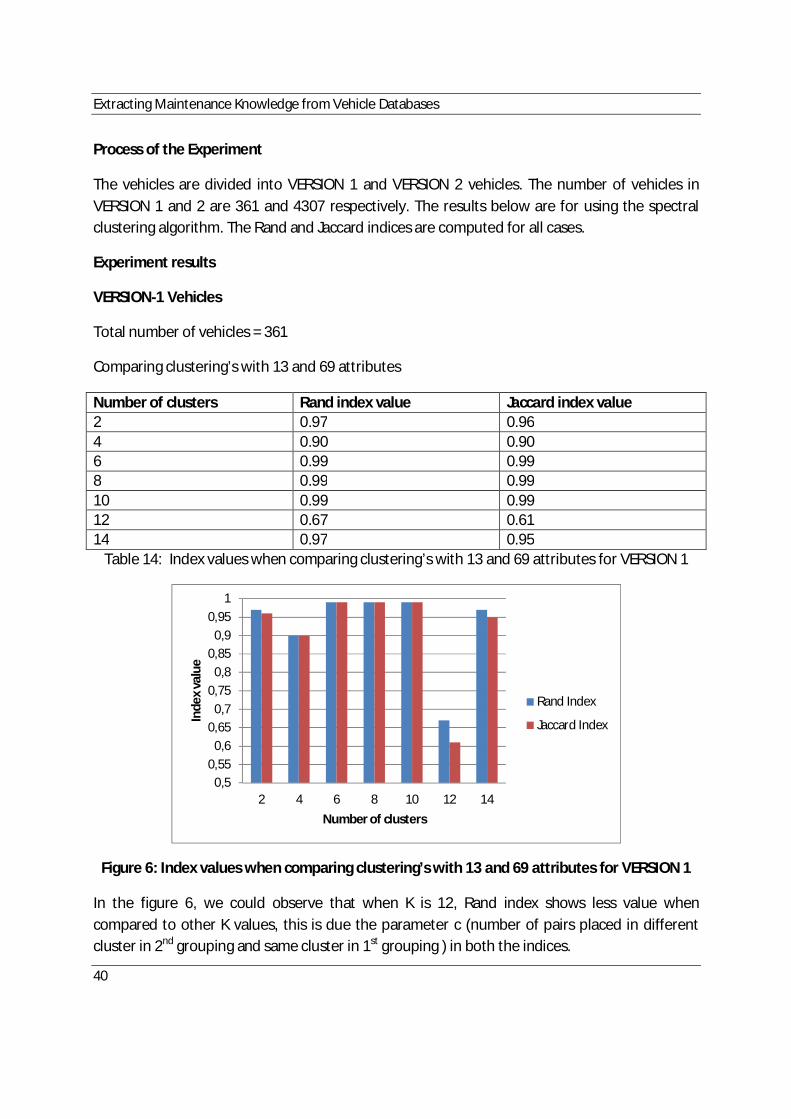
Extracting Maintenance Knowledge from Vehicle Databases
40
Process of the Experiment
The vehicles are divided into VERSION 1 and VERSION 2 vehicles. The number of vehicles in VERSION 1 and 2 are 361 and 4307 respectively. The results below are for using the spectral clustering algorithm. The Rand and Jaccard indices are computed for all cases.
Experiment results
VERSION-1 Vehicles
Total number of vehicles = 361
Comparing clustering’s with 13 and 69 attributes
Number of clusters Rand index value Jaccard index value 2 0.97 0.96 4 0.90 0.90 6 0.99 0.99 8 0.99 0.99 10 0.99 0.99 12 0.67 0.61 14 0.97 0.95
Table 14: Index values when comparing clustering’s with 13 and 69 attributes for VERSION 1
Figure 6: Index values when comparing clustering’s with 13 and 69 attributes for VERSION 1
In the figure 6, we could observe that when K is 12, Rand index shows less value when compared to other K values, this is due the parameter c (number of pairs placed in different cluster in 2nd grouping and same cluster in 1st grouping ) in both the indices.
0,50,55
0,60,65
0,70,75
0,80,85
0,90,95
1
2 4 6 8 10 12 14
Inde
x va
lue
Number of clusters
Rand Index
Jaccard Index

Results
41
The Figure 7 shows how the Rand and Jaccard indices behave when we compare two random clusterings into N number of clusters. We can see that the Jaccard index approaches 0 as N increases, and the Rand index approaches 1.
Figure 7: Rand and Jaccard index values when using random clusterings
In Figure 6 are the Rand and Jaccard index values almost the same. The basic difference between both indices is the variable d (the number of pairs that are placed in different clusters in both the clusterings), which is absent in Jaccard. In our clusterings is d zero in most cases, so that the Jaccard and Rand indices are equal.
Comparing clustering’s with 13 and all 425 attributes
Number of clusters Rand index value Jaccard index value 2 0.98 0.98 4 0.94 0.94 6 0.86 0.86 8 0.88 0.87 10 0.88 0.88

Extracting Maintenance Knowledge from Vehicle Databases
42
12 0.86 0.85 14 0.75 0.71 Table 15:Index values when comparing clustering’s with 13 and all 425 attributes for VERSION-1
Figure 8: Index values when comparing clustering’s with 13 and all 425 attributes for VERSION 1
Comparing clustering’s with 69 and all 425 attributes
Number of clusters Rand index value Jaccard index value 2 0.98 0.98 4 0.85 0.85 6 0.87 0.86 8 0.87 0.87 10 0.88 0.88 12 0.63 0.60 14 0.76 0.73
Table 16: Index values when comparing clustering’s with 69 and all 425 for VERSION 1
0,50,55
0,60,65
0,70,75
0,80,85
0,90,95
1
2 4 6 8 10 12 14
Inde
x va
lues
Number of clusters
Rand Index
Jaccard Index

Results
43
Figure 9: Index values when comparing clustering’s with 69 and all 425 for VERSION 1
VERSION-2 Vehicles
Total Number of vehicles = 4307
Comparing clustering’s with 13 and 69 attributes
Number of clusters Rand index value Jaccard index value 2 0.99 0.99 4 0.99 0.99 6 0.99 0.99 8 0.96 0.96 10 0.96 0.96 12 0.97 0.97 14 0.97 0.97
Table 17: Index values when comparing clustering’s with 13 and 69 attributes for VERSION 2
0,5
0,6
0,7
0,8
0,9
1
2 4 6 8 10 12 14
Inde
x va
lues
Number of clusters
Rand Index
Jaccard Index

Extracting Maintenance Knowledge from Vehicle Databases
44
Figure 10: Index values when comparing clustering’s with 13 and 69 attributes for VERSION 2
Comparing clustering’s with 13 and all 425 attributes
Number of clusters Rand index value Jaccard index value 2 0.99 0.99 4 0.99 0.99 6 0.99 0.99 8 0.98 0.98 10 0.98 0.98 12 0.97 0.97 14 0.98 0.98
Table 18: Index values when comparing clustering’s with 13 and all 425 attributes VERSION 2
Figure 11: Index values when comparing clustering’s with 13 and all 425 for VERSION 2
0,90,910,920,930,940,950,960,970,980,99
1
2 4 6 8 10 12 14
Inde
x va
lue
Number of clusters
Rand Index
Jaccard Index
0,90,910,920,930,940,950,960,970,980,99
1
2 4 6 8 10 12 14
Inde
x va
lue
Number of clusters
Rand Index
Jaccard Index

Results
45
Comparing clustering’s with 69 and all 425 attributes
Number of clusters Rand index value Jaccard index value 2 0.99 0.99 4 0.99 0.99 6 0.99 0.99 8 0.95 0.95 10 0.95 0.95 12 0.95 0.95 14 0.95 0.95 Table 19:Index values when comparing clustering’s with 69 and all 425 attributes for VERSION 2
Figure 12: Index values when comparing clustering’s with 69 and all 425 for VERSION 2
Discussion
The Rand index and Jaccard index results in Figure(6-12) show some interesting results, very close to one(bound is 0 to 1) for VERSION-2 vehicles, which means clustering using 13 attributes in Vehicle Specification is the same as those clustering results produced using 69 attributes. In other words, the vehicles in the clusters are almost the same when they are clustered using 13 attributes or 69 attributes.
We can also observe that, Rand index and Jaccard index values change quite a lot for VERSION-1 values when the numbers of clusters are more than 10. The reason is the fact that the number of VERSION-1 samples used is much less (361) when compared to the number of samples in VERSION-2(4307). As the number of VERSION-1 vehicles are showing sparse values of attributes and the number of clusters is more than 10, the results change drastically. When the number of vehicles is high, the results look quite consistent (based on VERSION-2 vehicles results). This indicates that 13 GTA attributes clustering results are very close to 69 attributes
0,90,910,920,930,940,950,960,970,980,99
1
2 4 6 8 10 12 14
Inde
x va
lues
Number of clusters
Rand Index
Jaccard Index

Extracting Maintenance Knowledge from Vehicle Databases
46
clustering results of these vehicles, and very close to using all the 425 attributes. We therefore chose to continue using only the 13 GTA parameters.
5.5 Cluster Validation results on Service Database (MSD)
The experiments so far were done on the Vehicle Specification Database and the modified PMI distance. Spectral clustering algorithm was used to cluster the vehicles.
This experiment described in this section done on the Maintenance Database to determine the optimal number of clusters [K] that we can use. In VSD the results indicated that 2-6 clusters show the same Rand index in most cases. Here we are changing the number of clusters K from 2 to 9 to see how the inter-cluster and intra-cluster distance varies (see section 4.6 on cluster validity). This will help us to determine the right number of clusters in MSD.
Purpose of the experiment:
The cluster validation for the maintenance database is performed to determine the optimal number of clusters in the database.
Process of the experiment:
The validity values for the Maintenance database are calculated by changing the number of clusters from 2 to 10. In order to check the consistency of the results, the samples are randomly divided into five subsets of equal size. Each subset is clustered ten times for every individual number of clusters. For example, a dataset (d1) is executed ten times for each K = 2, 3….10 (where K is the number of clusters).
To check how the validity measure works with binary representation of data, we have implemented the same measure with random data, synthetic data and our real data with the same number of samples. The random dataset is generated by presence (1) and absence (0) of all the 43 operations considered in the maintenance database for clustering. This random dataset does not have any cluster structure, it is just noise, and we do not expect to see any cluster structure indicated with the validity index.
The synthetic dataset is generated by randomly picking reference vehicles from our dataset and changing the values around those references. The intra cluster distance between the vehicles we picked is 0.00093 which means the vehicles inside the clusters are very close to each other. The inter cluster distance between the reference vehicles is 0.01308 that tells us that the distance between different reference vehicle clusters is high. We expect the cluster validity measure to indicate to us the correct number of clusters. These values indicate how clear the cluster structure is in our synthetic dataset. This will also tell us that clustering results produced

Results
47
are not random. The number of reference vehicles (in other words the number of clusters) in synthetic data we used is 4.
Figure 13: Validity values for Random, Synthetic and Real Data
Figure 13 shows the results of the synthetic, random and real dataset validity measure values respectively. According to the validity measure, the samples are clustered effectively when the value is closer to 0. The results indicate that our dataset (real data) is not a random dataset and there are natural groups present in it. For example, in synthetic dataset the validity value passes 1, when the number of clusters is more than 6 (we know the number of clusters is 4). In our dataset it passes 1 when K = 3. In the random dataset, the validity value increases drastically when the number of clusters is more than 1 and reaches 100 when K=2. This indicates to us that the number of clusters for our dataset is 3. The random sampling of our five different datasets also shows the natural number of clusters is 3 or 4.
The entire MSD dataset is divided into five equal subsets (1 to 5) to check whether the validity value gives consistent results over each subset.
Dataset Number: 1,2,3,4,5

Extracting Maintenance Knowledge from Vehicle Databases
48
Figure 14: Validity Values with Mean and SD for 1, 2, 3, 4, 5 dataset in MSD

Results
49
Discussion
Figure 14 show the Mean and Standard Deviation for each dataset. The mean and standard deviation values show that when the number of clusters is 3 and 4 the validity value is very close to 0 and 1. In datasets 1,2 and 5 the validity values crosses one when the number of clusters is 3 and in datasets 3, 4 the validity value crosses one when the number of clusters 4. The results indicate that 3 or 4 natural clusters are present in Maintenance databases and the results are determined with the help of binary representation of the database. The motivation for using binary representation of data is described in the next section.
5.6 Binary Representation of Data in MSD
The binary representation of the data is used in the Maintenance service database. The frequency representation of the data has also been implemented in this data. To compare, we have examined the clustering results of both the representations of data. The samples of how the maintenance database looks with these representations are shown in Figures 15 and 16.
Figure 15: Sample of Frequency representation of MSD

Extracting Maintenance Knowledge from Vehicle Databases
50
Figure 16: Sample of Binary representation of MSD
Figure 17: Clustering results using both binary and frequency representation
Results
51
Figure 17 shows the clustering results for a dataset with both representations. The inferences that can be drawn are:
1. The binary representation of the data shows consistent results by forming the evenly distributed clustered especially when the number of clusters is 2 and 3.
2. The frequency representation of the data also shows some evenly distributed clusters (close to binary representation of data) when the number of clusters is high (3, 4).
The frequency representation of data gives the number of times an operation occurs in the dataset. The binary representation of data gives the presence and absence of an operation in the dataset. In our analysis, if an operation has been done at least once then we will consider that vehicle in the particular operation category. So we have chosen to use binary representation of data since it gives only presence and absence of data.
5.7 Clustering Matrices between VSD and MSD
One of our goals is to see if there is any relation between the vehicle specification and the maintenance needs. After clustering is done in both the databases, we check whether the vehicles inside the clusters area almost the same. Do vehicles that have similar specifications, and are therefore grouped together in the clustering of VSD, end up in the same cluster in MSD?
Purpose of the experiment:
The clustering results obtained in both the databases are compared to determine whether there is any relationship between VSD and MSD.
Process of the experiment:
The databases MSD and VSD are clustered with the number of clusters K= 2,3,4,5. The clustering results are compared to each other to find whether the vehicles fall in the same clusters in both the databases. The Rand index values are calculated for each pair of K values.
Experiment Results:
The clustering matrices for 2, 3, 4 and 5 clusters are obtained. The following table shows the results for the same set of vehicles. The results are shown for only one subset of vehicles (765) out of five subsets but results are very similar for the other subsets. The clusters of VSD are denoted as C1, C2, C3, C4 and C5. The clusters of MSD are denoted as K1, K2, K3, K4 and K5 to make the distinction clear.
The clustering matrices represent both Maintenance Service Database (MSD) clustering details of number of vehicles (In the first column) and Vehicle Specification Database (VSD) clustering
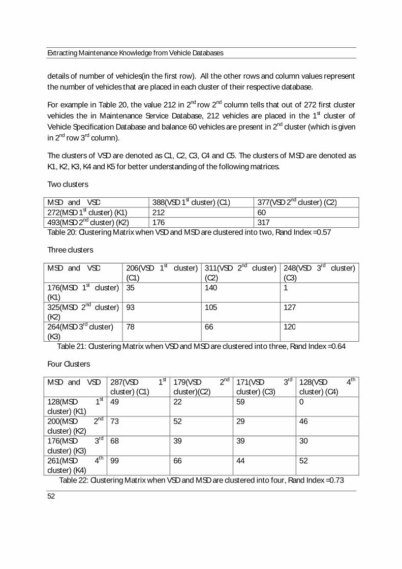
Extracting Maintenance Knowledge from Vehicle Databases
52
details of number of vehicles(in the first row). All the other rows and column values represent the number of vehicles that are placed in each cluster of their respective database.
For example in Table 20, the value 212 in 2nd row 2nd column tells that out of 272 first cluster vehicles the in Maintenance Service Database, 212 vehicles are placed in the 1st cluster of Vehicle Specification Database and balance 60 vehicles are present in 2nd cluster (which is given in 2nd row 3rd column).
The clusters of VSD are denoted as C1, C2, C3, C4 and C5. The clusters of MSD are denoted as K1, K2, K3, K4 and K5 for better understanding of the following matrices.
Two clusters
MSD and VSD 388(VSD 1st cluster) (C1) 377(VSD 2nd cluster) (C2) 272(MSD 1st cluster) (K1) 212 60 493(MSD 2nd cluster) (K2) 176 317 Table 20: Clustering Matrix when VSD and MSD are clustered into two, Rand Index =0.57
Three clusters
MSD and VSD 206(VSD 1st cluster) (C1)
311(VSD 2nd cluster) (C2)
248(VSD 3rd cluster) (C3)
176(MSD 1st cluster) (K1)
35 140 1
325(MSD 2nd cluster) (K2)
93 105 127
264(MSD 3rd cluster) (K3)
78 66 120
Table 21: Clustering Matrix when VSD and MSD are clustered into three, Rand Index =0.64
Four Clusters
MSD and VSD 287(VSD 1st cluster) (C1)
179(VSD 2nd cluster)(C2)
171(VSD 3rd cluster) (C3)
128(VSD 4th cluster) (C4)
128(MSD 1st cluster) (K1)
49 22 59 0
200(MSD 2nd cluster) (K2)
73 52 29 46
176(MSD 3rd cluster) (K3)
68 39 39 30
261(MSD 4th cluster) (K4)
99 66 44 52
Table 22: Clustering Matrix when VSD and MSD are clustered into four, Rand Index =0.73

Results
53
Five Clusters
MSD and VSD
(VSD 1st cluster) (C1) 148
(VSD 2nd cluster) (C2) 159
(VSD 3rd cluster) (C3) 160
(VSD 4th cluster) (C4) 159
(VSD 5th cluster) (C5) 128
281 (MSD 1st cluster) (K1)
42 50 69 63 57
116 (MSD 2nd
cluster) (K2)
45 53 3 14 1
127 (MSD 3rd cluster) (K3)
21 19 31 30 26
87 (MSD 4th cluster) (K4)
18 23 13 21 12
154 (MSD 5th cluster) (K5)
22 25 44 31 32
Table 23: Clustering Matrix when VSD and MSD are clustered into five, Rand Index =0.66
These clustering matrices show that the databases are not perfectly matched (but this was not expected either). However, there is more common structure with three or four clusters (see also the Figure below).

Extracting Maintenance Knowledge from Vehicle Databases
54
Figure 18: Average Rand index values of 5 subsets from 2-6 clusters
Discussion:
Figure 18 gives the Rand index values of five different datasets calculated for different numbers of K values between the Maintenance (MSD) and Vehicle specification (VSD) database (when K is the same for both VSD and MSD). The Rand index values are less than 0.75 in all cases which indicates the clustering results are not matching very well. The Rand index values are, however, higher for 3 and 4 clusters in most datasets when compared to other K values.
5.8 Interesting results:
What constitutes an “interesting” result with the clustering matrices? This is when the groupings of the two databases match well. Hypothetical examples of interesting clustering matrices are shown in the following tables:
Ideal case: 1
MSD and VSD 176(VSD 1st cluster) (C1)
325(VSD 2nd cluster) (C2)
264(VSD 3rd cluster) (C3)
176(MSD 1st cluster) (K1)
176 0 0
325(MSD 2nd cluster) (K2)
0 325 0
264(MSD 3rd cluster) (K3)
0 0 264
Table 24: Matrix of ideal case-1 for expected results, Rand index =1
0,30,35
0,40,45
0,50,55
0,60,65
0,70,75
0,8
1st set 2nd set 3rd set 4th set 5th set
Inde
x va
lue
Rand Index
2 clusters
3 clusters
4 clusters
5 clusters
6 clusters

Results
55
Table 24 has very good results (examples) where all the clusters in both the databases are clustered perfectly and we can confidently say that Vehicle Specification (VSD) and Maintenance Service (MSD) databases are correlated. The Rand index value for this clustering matrix is 1 since there is a perfect correlation between the database clusters. This means that the same types of vehicles have the same problems, i.e. the maintenance problems of the vehicles can be predicted from the vehicle specification.
Ideal case: 2
MSD and VSD 176(VSD 1st cluster) (C1)
325(VSD 2nd cluster) (C2)
264(VSD 3rd cluster) (C3)
195(MSD 1st cluster) (K1)
166 5 24
320(MSD 2nd cluster) (K2)
0 320 0
250(MSD 3rd cluster) (K3)
10 0 240
Table 25: Matrix of ideal case-2 for expected results, Rand index = 0.83
This second case of clustering matrix have interesting results in terms of number of vehicles in one cluster is very high and some little number of vehicles are placed in another cluster in other database.
5.9 Clustering Matrix after changes
To possibly improve the clustering of MSD, the operations groups were reviewed. We tested clustering after removing one operation group at a time and examined how the results changed. (See Table 11 for operation groups.)
The motivation for doing this was that some operation groups could be noisy, e.g. faults that occurred for reasons that were not related to vehicle use or specification.

Extracting Maintenance Knowledge from Vehicle Databases
56
Figure 19: Rand Index values when different operation groups are removed-Part A
(Arrow Mark in the y-axis shows the index values before these operation groups removed)
Figure 20: Rand Index values when different operation groups are removed-Part B
(Arrow Mark in the y-axis shows the index values before these operation groups removed)
The number of clusters K = 3 is used to cluster the vehicles, since 3 and 4 show better Rand index results (Figure 18).Figure 19 shows the Rand index values of five different datasets when operations groups like clutch, sensor, absorber, filter and coolant are removed. We observed that, Rand index values when those operation groups are removed are higher than 0.8 in many
0,6
0,65
0,7
0,75
0,8
0,85
0,9
0,95
1
1st set 2nd set 3rd set 4th set 5th set
Inde
x va
lue
Rand Index(after removed operations)
clutch operations
Sensor operations
Absorber operations
Filter operations
Coolant operations
0
0,1
0,2
0,3
0,4
0,5
0,6
0,7
0,8
1st set 2nd set 3rd set 4th set 5th set
Inde
x va
lue
Rand Index(after removed operations)
Engine operations
Brakes operations
Oil and V-rod operations

Results
57
cases, which is considerably higher than the index values when operation groups are not removed (Figure 18).
On the other hand, when groups like engine, brake, oil and V-rod operations are removed (Figure 20) the Rand index values decrease or similar to the results shown in Figure 18. So the operations groups like engine, brake, oil and V-rod operations are not removed and we considered them as important operation groups. The arrow mark in the Y-axis in both Figure 19 and Figure 20 indicates the index values before removing any operation group. The clustering matrices, when different operation groups are removed are given below. We refer to Table 11 for the different operations groups considered.
Clustering matrix (when clutch operations are removed and K=3 for both VSD and MSD)
MSD and VSD 212(VSD 1st cluster) (C1) (Constant GTA attributes except GCW, Propeller shaft and engine values)
138(VSD 2nd cluster) (C2) (Constant GTA attributes except engine and propeller shaft values)
415(VSD 3rd cluster) (C3) (Constant GTA attributes except brakes and axle type values)
451(MSD 1st cluster) (K1) (mostly contains engine and brake problems)
179
13 259
136(MSD 2nd cluster) (K2) (mostly contains filter and sensor related problems)
12 124 0
178(MSD 3rd cluster) (K3) (mostly absorber and brake problems)
21 1 156
Table 26: Clustering Matrix when clutch operations are removed, Rand index = 0.83

Extracting Maintenance Knowledge from Vehicle Databases
58
Description
There are 451 vehicles in the 1st cluster of MSD (Table 26) and these vehicles are placed largely in two different clusters in VSD with 179 and 259. When there service profiles are observed they mostly had brake, engine and filter problems. When these vehicles were looked into their VSD (13 GTA attributes) the changes comes from the attributes Gross Combination Weight, Propeller Shaft and two different engine values, whereas other attributes are constant. In the second cluster which has 136 vehicles in MSD and contains filter and sensor related problems which had almost the same configuration of attributes except engine and propeller shaft values. The third cluster in MSD has 178 vehicles which contain absorber and brake problems, which indeed changes in attributes like brakes, axle type in VSD.
Clustering matrix (when sensor operations are removed and K=3 for both VSD and MSD)
MSD and VSD 230(VSD 1st cluster) (C1) (Constant GTA attributes except brakes and propeller shaft)
166(VSD 2nd cluster) (C2) (Constant GTA attributes except GCW ,Transmission values)
369(VSD 3rd cluster) (C3) (Constant GTA attributes except type of brakes, propeller shaft)
231(MSD 1st cluster) (K1) (mostly contains oil, filter and engine problems)
223 0 8
257(MSD 2nd cluster) (K2) (mostly contains brake and engine related problems)
4 147 106
277(MSD 3rd cluster) (K3) (mostly contains clutch, absorber and
3 19 255

Results
59
brake problems)
Table 27: Clustering Matrix when sensor operations are removed, Rand index = 0.82
Description
When sensor operations are removed (Table 27), the number of vehicles clustered three different clusters is 231,257 and 277 in MSD respectively. When these vehicles are looked into their respective service database 1st cluster had problems like oil, filter and engine problems, 2nd cluster contains problems related to brakes, engines and some gear problems and 3rd cluster vehicles has problems like clutch, absorber and brake problems. When these three different MSD clusters are looked into their respective Vehicle specification database the clustering differences comes from their engine type, transmission and type of brakes.
Clustering matrix (when absorber operations are removed and K=3 for both VSD and MSD)
MSD and VSD 183(VSD 1st cluster) (C1) (Constant GTA attributes except bogie type and engine values)
246(VSD 2nd cluster) (C2) (Constant GTA attributes except propeller shaft and transmission type)
336(VSD 3rd cluster) (C3) (Constant GTA attributes except axle load and brake types)
94(MSD 1st cluster) (K1) (contains mostly clutch and filter problems)
0 94 0
162(MSD 2nd cluster) (K2) (contains engine and oil leak problems)
2 129 31
509(MSD 3rd cluster)
181 23 305

Extracting Maintenance Knowledge from Vehicle Databases
60
(K3) (contains brake, sensor and V-rod problems )
Table 28: Clustering Matrix when absorber operations are removed, Rand index = 0.78
Description
When absorber operations are removed (Table 28) from the MSD, the first cluster of MSD has 94 vehicles and those vehicles are placed in 2nd cluster of VSD. When these vehicles are looked at separately, almost all the vehicles have the same configuration, except changes exist in the propeller shaft and transmission type. In service databases these vehicles have clutch and filter problems. In the third cluster of MSD we have 509 vehicles (these vehicles have problems like sensor and brake problems) which are placed in two different clusters in VSD and they change in the attributes like bogie type and Front and Rear axle Load.
Discussion
The clustering matrices shown in Tables 26, 27, 28and Rand index values shown in Figure 19 and 20 after removing operation groups look quite promising. We can make use of this method to determine the operation groups that are important from a maintenance perspective. The clustering matrices give an idea of how the vehicles are clustered in both the databases. The type of vehicles in those clusters and kind of problems occurred to those vehicles can be understood. By carefully changing and selecting the operations (Rand index could be used to select the operation groups) from Maintenance Service Databases there are indications of interesting patterns that can be extracted with these two databases.
5.10 Data Mining Rules on Vehicles
The clustering results of VSD are further used to determine the entropies of all the 13 GTA attributes for extracting decision making rules. The decision tree algorithm is used to label the vehicles of different clusters based on their 13 GTA attributes. In other words, this decision tree will tell us which VSD cluster it belongs. The number of vehicles considered for this decision tree is 4215 (tractors) out of 4668, since rigid type vehicles are less in number and have more different attributes than tractors.
The decision tree is built when the Vehicle Specification Database is clustered into three clusters. This will aid us to know the attributes that play a vital role in this classification of vehicles (in other words how these clusters are represented or labeled inside the clusters). The decision tree (the C4.5 algorithm [40]) is built based on the attributes entropy values. The

Results
61
decision tree obtained is given below. For instance, if a new vehicle is given with the following attributes, we can describe how the service profile of the vehicle will look like by using this decision tree.
Figure 21: Decision Tree for Vehicle Specification Database (Using Entropy)
This decision tree (Figure 21) can be used to label the vehicles based on these GTA attributes. If we give a new vehicle, we can use this tree to determine which cluster it belongs (C1, C2, C3). Using this, we can provide the service profile for that respective vehicle by having K1, K2, K3 clusters in MSD.
For example, if a vehicle has attributes RAL19, FAL9.0 then it belongs to cluster number 3. Now, using these C1, C2 and C3 we can give their respective service profiles of K1, K2 and K3 of service database clusters. Our dataset is divided into equal subsets randomly to test whether this decision tree satisfies. The results have shown the same attribute decision tree gives less entropy values when compared to other attributes in the vehicles.
The maintenance problems of vehicles present for the same vehicle specification clusters are extracted. The service profiles for the vehicles belong to these three (C1, C2, C3 of VSD) clusters are shown in Figure 22 and 23.
All Vehicles
RAL 19 OTHER RAL VALUES
FAL 7.1 FAL 8.0 FAL 9.0
PLM 0975,1425 PLM 1150,1075,1125, 1000, 1200, 925,950
PLM 0850,1050,1175,
D12D420 D12D460
C2 C1
PLM 1025, 0850, 1050
C3
C3 PLM 1000,1200
C1
C2
PLM 950, 1125, 975, 1075, 1375, 1150, 1425, 1175, 1250, 1450,
C3 C1 C2
C1,C2,C3 are the clusters of VSD when K = 3

Extracting Maintenance Knowledge from Vehicle Databases
62
Figure 22: Histogram of Service Profiles of VSD for 3 clusters
Figure 23: Graph of Service Profiles of VSD for 3 clusters
Using the service profiles of the vehicles for three different clusters (C1, C2 and C3) of VSD, various rules are extracted (for MSD clusters K1, K2, K3) and they are presented in Table 29.
Rules VSD MSD 1 If vehicles belongs to Cluster 1
(C1) Operations like Engine starting difficulties(11),Engine oil change(21), Gear box oil change(23) are high
2 If vehicles belongs to Cluster 2 (C2)
Operations likeD12D Engine problems(4), Oil Cooler Replace(33),Engine Noise(7),NSR Brake Replace(16), Brake pads replace(17),Gearbox Replace(18) are high
0 5 10 15 20 25 30 35 40 450
50
100Service Profile for 3 Clusters
0 5 10 15 20 25 30 35 40 450
50
100
0 5 10 15 20 25 30 35 40 450
20
40
60
X Axis - Different Operations Y Axis - Percentage of MaintenanceProblems
0
20
40
60
80
100
120
1 3 5 7 9 11 13 15 17 19 21 23 25 27 29 31 33 35 37 39 41 43
Perc
enta
ge(%
)
Different Operations
Cluster 1 Cluster 2 Cluster 3

Results
63
and generally have more problems compared to Cluster 3 vehicles
3 If vehicles belongs to Cluster 3 (C3)
Operations Shock Absorber Replace(35) is high and generally have less problems compared to Cluster 2 vehicles
Table 29: Data Mining Rules for Vehicles
5.11 PMI and Modified PMI
Purpose of the Experiment
This experiment is done to investigate whether there is a change in the clustering results when using PMI and the modified PMI.
Process of the Experiment
We clustered the VSD data set into the same three clusters (Spectral clustering) by using both the original and the modified PMI. The maintenance service profiles for both PMI measures are presented below.
Experiment Results
Figure 24: Service profile of vehicles with PMI
0
20
40
60
80
100
120
1 3 5 7 9 11 13 15 17 19 21 23 25 27 29 31 33 35 37 39 41 43
Perc
enta
ge(%
) of M
aint
enan
ce P
robl
ems
Different Operations
Cluster 1 Cluster 2 Cluster 3

Extracting Maintenance Knowledge from Vehicle Databases
64
Figure 25: Service profile of the vehicles with Modified PMI
Figure 24 and 25shows service profiles for both PMI’s. We can observe the changes in the percentage of problems to the vehicles when compared to the old PMI. Operations like 1,5,25 and 41 show some considerable changes (Figure 25). This indicates to us that clustering results of VSD shows slight changes that we can observe in the service profiles when using old and modified PMI’s. These changes to PMI will improve the clustering results in these databases.
We also compared the correlation results (transition matrices with VSD and MSD) with modified PMI. The results show that there is not much change in the rand index values obtained before and after the PMI calculation changed.
5.12 Comparison Results of Clustering Algorithms
The clustering algorithms are compared with all the datasets in the Maintenance Services Database. The results show that spectral clustering gives high validity measure values out of three algorithms. The validity values are much closer to zero when datasets are clustered into 3 and 4 (natural number of clusters that we found). The Single Linkage Clustering algorithm shows different clustering results when compared to Spectral Clustering and K-means. Each of the five datasets is clustered with all the three algorithms. Figures below shows the clustered results in terms of number of vehicles (for one dataset which contains 765 samples) clustered in each cluster for 2 to 5 clusters. Figure 26 shows the clustering results with the three clustering algorithms.
0
20
40
60
80
100
120
1 3 5 7 9 11 13 15 17 19 21 23 25 27 29 31 33 35 37 39 41 43
Perc
enta
ge(%
) of P
robl
ems
Different Operations
Cluster 1 Cluster 2 Cluster 3

Results
65
Figure 26: Comparing algorithms when number of clusters are 2,3,4,5 using MSD

Extracting Maintenance Knowledge from Vehicle Databases
66
The result from Figure 26 indicates that Spectral Clustering and K-means are better when compared to the Single Linkage clustering algorithm. For example, when one dataset of 765 vehicles are clustered into two clusters (see Figure 25) single linkage clustering algorithms gives us one big cluster and one cluster with only one sample, whereas the other two clustering methods give more balanced clusters. This agrees with the conclusions in [21], that clustering results produced by the partitional approach are consistently better than those produced by the agglomerative approach. In experiments done in [22], a confusion matrix analysis shows that Hierarchical agglomerative clustering is unable to distinguish the largest clusters.

Analysis and Discussion
67
Chapter 6: Analysis and Discussion
6.1 Critical Attributes and Operations for Vehicles
The 13 GTA attributes that we considered in the Vehicle Specification Database are critical for every truck or large vehicle. By using these attributes, the clustering of the vehicles in any OEM Specification Database can be done.
The Operations that are taken into account in Maintenance Service Databases are based on the general perspective of how the vehicle works (example: brakes, clutch), parts that are considered to be costlier to replace (Engine) etc. This information can be used by any organization to determine their relationship between these two databases to improve their vehicle specification or their service planning.
6.2 Need for Previous Knowledge on Vehicles
The resulting clusters of Maintenance Service Database can be improved by having some previous knowledge on how the vehicle works internally and their critical parts. Since the method used here is sensitive to slight change in the presence and absence of the operations (refer to the section 5.8 which shows how the Rand index values changes when different operations groups are removed) it is considered that some vehicle knowledge is required.

Conclusion
68
Chapter 7: Conclusion
From the clustering matrix results, there is a relationship between the maintenance problems that occur in the vehicles and the vehicle specification (given that the vehicle attributes and maintenance operations are carefully selected). We can use the Rand index to determine important operations groups that can be considered for clustering the maintenance database. The natural number of clusters present in the databases can also be determined using a validity measure (and in this case they seem to be 3-4).
The different service profiles of maintenance problems with respect to their vehicle specification are presented. The decision tree rules based on the VSD attributes of the vehicles presented can be useful to determine the maintenance needs for the vehicles. If a new vehicle with the 13 GTA attributes is given, we can determine which VSD cluster it will most likely belong to and how the typical service profile of the vehicle will look like.
The validation results of clustering algorithms have shown that 13 GTA attributes is sufficient for clustering VSD. These attribute groupings will help us to understand the important attributes and determine different types of vehicles available in the database.
The clustering algorithms (Spectral clustering, K-means and Single Linkage Clustering) are compared using these databases and clustering validation results indicate that the Spectral clustering algorithm works better followed by K-means (number of vehicles per cluster is very different for Single Linkage compared to the other two algorithms which shows its inefficiency towards this kind of binary representation of data).
The binary representation of data and frequency representation is implemented on a maintenance service database. The binary representation of data is preferred since its best suited to our databases. The different distance measures to determine the distance between two lists (vehicles in our case) and how the PMI (Positive Matching Index) is different from them is discussed. The distance measure calculation of PMI is also changed to suit these kinds of databases and results show that there is a slight change.
The outlier results show that the number of services for a vehicle does not completely depend on the age and mileage of the vehicles.
The proposed method can also be used to extract information from a different vehicle (truck) specification and maintenance service databases of any OEM using their respective operation codes for services.

Conclusion
69
Chapter 8: Future Work
By using the results provided in this thesis, the following work can be added in the future to improve maintenance service needs of vehicles.
1. Determining whether the service profiles of the vehicles obtained using these two databases have any relation with the Logged Vehicle Database(LVD) that contains some information about how the vehicles are being used.
2. Determining whether refinement of vehicle attributes and maintenance operations used will improve these service profiles. For example, if an intermediate representation between binary and frequency can improve.
3. It would be interesting to investigate how these databases information and knowledge can be used to improve the service schedules of OEM.

Extracting Maintenance Knowledge from Vehicle Databases
70
Chapter 9: References
[1] Sean Lyden. Smart Strategies for Extending Medium-Duty Truck Replacement Cycles. Work Truck Magazine; November 2011.
[2] Pedro Bastos, Rui Lopes, Luis Pires, Tiago Pedrosa. Maintenance behavior based prediction system using Data Mining. IEEE International Conference on Industrial Engineering and Engineering Management. Braganca, Portugal; 2009; p. 2487- 2491.
[3] Harding JA, Shahbaz M, Srinivas and Kausiak A. Data Mining in Manufacturing: A Review. American Society of Mechanical Engineers (ASME), Journal of Manufacturing Science and Engineering; 2006; p. 969-976.
[4] Harding JA, Chowdary AK and Tiwari MK. Data Mining in Manufacturing: review based on the kind of knowledge. Journal of Intell. Manufacturing; 2009; p. 501-521.
[5]Skormin VA, Gorodetski VI and PopYack IJ. Data mining technology for failure of prognostics of avionics. IEEE Transactions on Aerospace and Electronic systems, 2002; p. 388-403.
[6] Romanowski CJ, Nagi R. On comparing bills of materials: A similarity/distance measure for unordered trees. IEEE Transactions on system man and cybernetics part-A, 2005; p. 249-260.
[7] Sylvain L, Fazel F, Stan M. Data Mining to Predict Aircraft Component Replacement. IEEE Intelligent Systems 14(6). 1999; p. 59-65.
[8] Brett Edwards, Micheal Zatorsky, Richi Nayak. Clustering and Classification of Maintenance Logs using Text Data mining. Seventh Astralasian Data Mining Conference, Glenelg, Australia; 2008.
[9] Thomas Grubinger and Nicholas Wickström. Knowledge extraction from real-world logged truck data. SAE Int. J. Commer. Veh. 2(1): 64-74; 2009.
[10] Adeel Tariq, Irfan Anjum Manarvi. Defect Trend Analysis of F-7P Aircraft through Maintenance History. IEEE Aerospace Conference, Big Sky, Montana; 2011; p. 1-8.
[11] Nasrullah Khan and Irfan Anjum Manarvi. Identification of Delay Factors in C-130 Aircraft Overhaul and Finding Solutions through Data Analysis. IEEE Aerospace Conference, Big Sky, Montana; 2011; p. 1-8.
[12] Bilal Younes and Irfan Anjum Manarvi. Defect Trent Analysis of Airborne fire control Radar using Maintenance History. IEEE Aerospace Conference; Big Sky, Montana; 2011; p. 1-15.

References
71
[13] Tahir Bashir and Irfan Anjum Manarvi. Defect Trend Analysis of Air Traffic Control Radars. IEEE Aerospace Conference; 2012; p. 1-5.
[14] Zaluski Marvin, Letourneau Sylvain, Bird Jeff et.al. Developing Data Mining-Based Prognostic Models for CF-18 Aircraft, Journal of engineering for gas turbines and power transactions of asme; 2011.
[15] Hong Kyu Han, Hong Sik Kim, So Young Sohn. Sequential association rules for forecasting failure patterns of aircrafts in Korean air force. Expert System with Applications 2009; p. 1129-1133.
[16] Satnam Singh, Pinion C, Subramania HS. Data-Driven Framework for Detecting Anomalies in Field Failure Data. IEEEAC paper #1221, Version 2; Updated January 3 2011.
[17] Liqiang Geng and Howard J Hamilton. Interestingness Measures for Data Mining: A Survey. University of Regina, ACM Computing Surveys, Vol. 38, Article 9; 2006.
[18] Usama Fayyad, Gregory Piatetsky-Shapiro, Padhraic Smyth. From Data Mining to Knowledge Discovery in Databases. AI Magazine Volume 17 Number 3; 1996.
[19] Jain AK, and Dubes RC. Algorithms for Clustering Data. Englewood Cliffs, NJ: Prentice-Hall; 1988
[20] Osama Abu Abbas. Comparison between data clustering algorithms. Yarmouk University, Jordan: The International Arab Journal of Information Technology; July 2008.
[21] Ying Zhao and George Karypis. Comparison of Agglomerative and Partitional Document Clustering Algorithms. Department of Computer Science, University of Minnesota, Minneapolis; MN 55455.
[22] Marina Meila and David Heckerman. An Experimental Comparison of Several Clustering and Initialization Methods. Microsoft Research Technical Report; 1998.
[23] Manish Verma, Mauly Srivastava, Neha Chack, Atul Kumar Diswar, Nidhi Gupta. A Comparative Study of Various Clustering Algorithms in Data Mining. International Journal of Engineering Research and Applications (IJERA); Vol. 2, June 2012; p. 1379-1384.
[24] Ulrike von Luxburg. The Tutorial on Spectral Clustering. Max Planck Institute for Biological Cybenetics; Statistics and Computing, 17(4); 2007.
[25]Sokal RR, Sneatho PHA. Numerical Taxonomy: The Principles and Practice of Numerical Classification. W.H. Freeman and Company, San Francisco; 1973.

Extracting Maintenance Knowledge from Vehicle Databases
72
[26] Goodman LA, Kruskal WH. Measures of association for cross classifications. Journal of the Americal Statistical Association; 1954. p. 732-764.
[27] Seung-Seok Choi, Sung-Hyuk Cha, Charles C. Tapper. A Survey of Binary Similarity and Distance Measures. Journal on Systemics, Cybernetics and Informatics, Volume 8; 2010; p. 43-48.
[28] Tullos, R.E. Assessment of similarity indices for undesirable properties and a new tripartite similarity index based on cost function. In: Palm, Chapela (Eds.), Mycology in Sustainable Development. Boone NC, USA; 1997; p. 122- 143.
[29] Deutsch R, Cherner M, Grant I. Significance testing of a cluster of multivariate binary variables: Comparison of the tripartite T index to three common similarity measures; 2006.
[30] Daniel Andres Dos Santos, Reena Deutsch. The Positive Matching Index: A new similarity measure with optimal characteristics. Pattern Recognition Letter 31, University of California; San Diego, USA; 2010.
[31] Marina Meila. Comparing Clustering – An Axiomatic View. Proceedings of the 22nd International Conference on Machine Learning; Bonn, Germany; 2005.
[32] Marina Meila. Comparing Clustering- an information based distance. Journal of Multivariable Analysis. Department of Statistics, University of Washington; Box 354322, Seattle, USA; 2007; p. 873-895
[33] Lawrence Hubert and Phipps Arabie. Comparing Partitions. Journal of Classification; Springer-Verlag New York Inc.; 1985.
[34] E.B. Fowlkes and C.L.Mallows. A Method for Comparing Two Hierarchical Clusterings. Journal of the American Statistical Association, Vol.78, No.383; September 1983; p. 553-569.
[35] Glenn W. Malligan and Martha C. Cooper. A Study of the Comparability of External Criteria for Hierarchical Clustering Analysis. Multivariate Behavioral Research; 1986; p. 441-458.
[36] Janos Podani, Attila Engloner, Agnes Major. Multilevel Comparison of Dendograms: A new method with an application for Genetic Classifications. Statistical Applications in Genetics and Molecular Biology; Volume 8, Issue 1, Article 22; 2009.
[37] Silke Wagner and Dorothea Wagner. Comparing Clusterings – An Overview. January 12; 2007.

References
73
[38] Bashir ahamed Fardin Momin. Clustering and Validation for Very Large Databases. International Conference on Information and Automation, Shandong; December 2006; p. 258-263.
[39] Toi Li. A General Model for Clustering Binary Data. Proceedings of the eleventh ACM SIGKDD international conference on Knowledge discovery in data mining, NY, USA; 2005; p. 188-197.
[40] Quinlan JR.C4.5 Programs for Machine Learning. San Mateo, CA Morgan Kaufmann; 1993.
[41] Alan H.Cheetham and Joseph E.Hazel. Binary (Presence-Absence) Similarity Coefficients. Journal of Paleontology; Vol.43, No.5; September 1969; p. 1130-1136.
[42] Micheal Goebel, Le Gruenwald. A Survey of Data Mining and Knowledge discovery software tools. Department of Computer Science; University of Auckland; New Zealand.
[43] Arik Azran. A Tutorial on Spectral Clustering. Department of Engineering, University of Cambridge.
[44] Matlab Document website, Clustering Tools. K-means Clustering. Retrieved from http://www.mathworks.se/help/toolbox/stats/kmeans.html.
[45]Wikipedia a free encyclopedia on Clustering Analysis, Retrieved from http://en.wikipedia.org/wiki/Cluster_analysis.
[46] Dan Braha(Ed). Data Mining for Design and Manufacturing. Springer; 2002; p. 544, Hardcover.


HALMSTAD UNIVERSITY • PO Box 823 • SE-301 18 Halmstad, Sweden • www.hh.se