Embed Size (px)
Citation preview

Czech Technical University in Prague
Faculty of Nuclear Sciences and Physical Engineering
MASTER’S THESIS
Anyons and Their Significance
in Quantum Mechanics
and Statistical Physics
2011 Vaclav Zatloukal

Contents
1 Introduction 3
2 Genesis and the basic properties of anyons 5
2.1 Quantum statistics in d dimensions . . . . . . . . . . . . . . . . . . . . . . 6
2.1.1 Configuration spaces for identical particles . . . . . . . . . . . . . . 6
2.1.2 Path integral quantization in two dimensions . . . . . . . . . . . . . 9
2.2 Quantum formalism for anyons . . . . . . . . . . . . . . . . . . . . . . . . 11
2.2.1 Two-anyon problem . . . . . . . . . . . . . . . . . . . . . . . . . . . 13
2.3 Fractional statistics . . . . . . . . . . . . . . . . . . . . . . . . . . . . . . . 15
3 Anyons in experiments 18
3.1 Quantum Hall effect . . . . . . . . . . . . . . . . . . . . . . . . . . . . . . 18
3.1.1 Electron gas confined to two dimensions . . . . . . . . . . . . . . . 19
3.1.2 Planar electron in a magnetic field . . . . . . . . . . . . . . . . . . 21
3.1.3 Many-particle states . . . . . . . . . . . . . . . . . . . . . . . . . . 26
3.1.4 Quasiparticles in the fractional QHE . . . . . . . . . . . . . . . . . 28
3.1.5 Hall plateaux . . . . . . . . . . . . . . . . . . . . . . . . . . . . . . 31
3.2 High-temperature superconductivity . . . . . . . . . . . . . . . . . . . . . . 32
4 Propagation of anyons on the toric code 33
4.1 Toric code – introduction . . . . . . . . . . . . . . . . . . . . . . . . . . . . 33
4.2 Toric code Hamiltonian and anyonic excitations . . . . . . . . . . . . . . . 37
4.2.1 Stability of a quantum memory . . . . . . . . . . . . . . . . . . . . 38
4.2.2 Anyonic statistics revealed . . . . . . . . . . . . . . . . . . . . . . . 39
4.2.3 Perturbation induced anyonic quantum walks . . . . . . . . . . . . 40
4.3 Ladder lattice model . . . . . . . . . . . . . . . . . . . . . . . . . . . . . . 42
4.3.1 One anyon walk . . . . . . . . . . . . . . . . . . . . . . . . . . . . . 45
4.4 Continuous-time quantum walks in one dimension . . . . . . . . . . . . . . 48
1

4.4.1 Cyclic lattice . . . . . . . . . . . . . . . . . . . . . . . . . . . . . . 48
4.4.2 Infinite line . . . . . . . . . . . . . . . . . . . . . . . . . . . . . . . 51
4.4.3 Cyclic lattice with disordered couplings . . . . . . . . . . . . . . . . 54
4.5 Numerical results for one anyon walk on a periodic ladder lattice . . . . . . 57
4.5.1 Regular disorder – delocalization . . . . . . . . . . . . . . . . . . . 60
4.5.2 Random disorder – localization . . . . . . . . . . . . . . . . . . . . 61
5 Conclusion 66
A Braid group 67
A.1 Representations of the braid group . . . . . . . . . . . . . . . . . . . . . . 70
2

Chapter 1
Introduction
It is commonly accepted in physics that there are two kinds of particles in the three-
dimensional space — bosons and fermions. In statistical physics, bosons obey the Bose-
Einstein distribution law, while fermions are distributed among energy levels according
to the Fermi-Dirac distribution. In quantum mechanics, they differ by the phase factor
that the global wave function of a many-particle system acquires when two particles are
exchanged. The phase factor is +1 for bosons and −1 for fermions.
The key concept in these considerations is the principle of indistinguishability of iden-
tical particles. No quantum mechanical observable can distinguish between two particle
configurations that differ only by a permutation of identical particles. But what does the
word “permutation” or “exchange” of identical particles actually mean? And how to un-
derstand the notion of “identicalness”, anyway. In 1977, Leinaas and Myrheim [1] took
these questions seriously and found that whereas in three dimensions, indeed, only bosons
and fermions should exist, the two-dimensional space offers a whole continuous family of
possible quantum statistics. In two dimensions, one can consistently assign any phase fac-
tor eiα to reflect an exchange of two identical particles. Planar particles with these exotic
statistics were named anyons by Frank Wilczek.
We dedicate the Chapter 2 to explaining the ideas of Leinaas and Myrheim and to
formulating the basics of quantum mechanical description of anyons. The role of anyons
in statistical physics is also discussed. There have been several attempts to generalize the
bosonic and fermionic statistics, i.e. the number of particles that are allowed to occupy one
quantum state. We present the work of Haldane [2], who generalized the Pauli exclusion
principle in the way that the maximum number of particles that can occupy one quantum
state is anywhere between 1 (fermions) and ∞ (bosons). This so called fractional statistics
is, however, found to be incompatible with anyons defined through the exotic exchange
3

phase eiα when confronted with thermodynamical results for an ideal gas of anyons [3].
In Chapter 3, the anyons are explored from the experimental point of view. We discuss
how a two-dimensional system can be realized in practice and review the quantum Hall
effect to show that the quasiparticles that appear in the fractional quantum Hall system
exhibit exotic exchange statistics, i.e. that they are anyons [4]. Finally, we briefly overview
the high-temperature superconductivity, a yet unexplained phenomenon, in which anyons
were believed to take place as well. The experimental results, however, indicate that anyons
are currently observed only in the fractional quantum Hall effect.
In the last chapter, Chapter 4, we wander into the field of topological quantum compu-
tation. We introduce the Kitaev’s toric code [5], which is the most renowned topological
quantum error correcting code. It can serve as a quantum memory, robustness of which is
achieved on the physical (hardware) level. Anyonic excitations occur on the toric code as
local errors and if they propagate far enough, they cause logical errors, i.e. the quantum
information, stored in the quantum memory, is lost. Our objective is to investigate how
the nontrivial exchange statistics affects the continuous-time quantum walk of anyons on
the toric code. Especially, we would like to know whether a certain type of disorder in the
system causes Anderson localization [6] to take place as argued by Wootton and Pachos
[7].
4

Chapter 2
Genesis and the basic properties of
anyons
At the beginning of this chapter we focus on the theory of identical particles in a general
spatial dimension d. We show how the topology of configuration spaces of systems of
identical particles depend on the spatial dimension and what consequences a nontrivial
topology, expressed in terms of the fundamental group of a configuration space, has for the
concept of quantum statistics. Whereas in three and more dimensions only bosonic and
fermionic exchange statistics exist, in a two dimensional space the infinite connectedness
of the configuration space allows for much greater diversity. The phase factor that a wave
function acquires upon an exchange of two particles doesn’t have to be merely the bosonic
+1 or the fermionic −1, but can be, in principle, an arbitrary complex unit. The particles
in two dimensions are called anyons.
In the next part we formulate the Lagrangian and the Hamiltonian that incorporate the
general anyonic statistics. Based on the solution of the two-anyon problem, we argue that
free anyons (meaning without a direct force between them) exhibit a repulsive interaction
(similar in nature, but weaker than fermions) arising purely from their exchange statistics.
In statistical mechanics, bosons and fermions are described by distinct statistical distri-
butions over the energy states that they obey in thermal equilibrium — Bose-Einstein and
Fermi-Dirac distributions. The last section presents a generalization of these two possibil-
ities, the fractional statistics. The connection between anyons and the fractional statistics
is, however, not as straightforward. In fact, those two seem to be rather different concepts
— anyons don’t obey the fractional statistics.
5

2.1 Quantum statistics in d dimensions
Before we come to a proper discussion about the statistics, it is worth clarifying what
exactly one means by quantum statistics. In most textbooks on statistical mechanics,
the term “quantum statistics” refers to the phase picked up by a wave function when
two identical particles are interchanged, i.e. under the permutation of the particles. One
usually writes
ψ(x2,x1) = eiαψ(x1,x2) . (2.1)
But this is slightly misleading and has been correctly criticized in literature [8]. If the
particles are strictly identical then the word “permutation” has no physical meaning since
a given configuration and the one obtained by the permutation of particle coordinates are
merely two different ways of describing the same particle configuration. The two quantities
in equation (2.1) have no separate meaning and the equation therefore at most reflects a
redundancy in the notation.
The origin of the trouble lies in the introduction of the particle indices which brings ele-
ments of non-observable character into the theory and makes the discussion more obscure.
The term quantum statistics actually refers to the phase that arises when two particles are
adiabatically transported giving rise to the exchange. The principle of indistinguishability
of identical particles plays the central role and it has, as we shall see, profound physical
consequences.
2.1.1 Configuration spaces for identical particles
Following Khare [3] and Leinaas and Myrheim [1], let us enquire about the configuration
space of a system of identical particles. In statistical mechanics one normally considers the
full phase space, but it turns out that the configuration space is enough for this discussion.
Suppose one particle space is X. Then what is the configuration space of N identical
particles? The naive answer is XN , which, even though is true locally, is not correct
globally. Since the particles are strictly identical, there is no distinction between the
points in XN that differ only in the ordering of the particle coordinates.
For example, take the point
x = (x1,x2, . . . , xN) (2.2)
in XN , where xi ∈ X for i = 1, 2, . . . , N . Now consider another point x′ in XN which is
obtained from x by the permutation p of the particle indices, i.e.
x′ = p(x) = (xp(1), . . . , xp(N)) . (2.3)
6

Clearly, both x and x′ describe the same physical configuration of the system. Thus the
true configuration space of the N -particle system is not the Cartesian product XN , but
it is the quotient space XN/SN which is obtained by identifying the points of XN that
represent the same physical configuration, i.e. it is obtained by “dividing out” the action
of the symmetric (or permutation) group SN . Note that SN is a discrete and indeed finite
transformation group acting in XN . As a result, the space XN/SN is locally diffeomorphic
to XN except at the points
∆ =(x1, . . . , xN) ∈ XN | xi = xj for some i 6= j
, (2.4)
where two or more particles occupy the same position in X. For convenience, we remove
the points of ∆ from our configuration space1, i.e. the configuration space of N identical
particles becomes
(XN\∆)/SN . (2.5)
Since the spaces XN\∆ and (XN\∆)/SN are locally diffeomorphic, they are equivalent on
the classical level. However, on the quantum level global properties of the configuration
space are of deep physical significance as we shall see later when we will path-integral
quantize the system of identical particles.
Let us now study in detail the configuration space (XN\∆)/SN under the assumption
that the one particle configuration space X is the d–dimensional Euclidean space Rd,
d = 1, 2, 3, . . .. Let us take, for simplicity, the two particle case (N = 2), i.e. the space
((Rd × Rd)\∆)/S2. Using the center-of-mass coordinate
xc.m. =x1 + x2
2(2.6)
and the relative coordinate
xr = x2 − x1 , (2.7)
where x1,x2 ∈ Rd are the coordinates of the individual particles, we can see that removing
the set of coincidence ∆ from our configuration space is expressed by the condition xr 6= 0.
The identification of the points (x1,x2) and (x2,x1) corresponds to identifying the points
(xc.m., xr) and (xc.m.,−xr). Therefore the configuration space of two identical particles
reads
((Rd × Rd)\∆)/S2 = Rd × (Sd−1/S2)× (0, +∞) , (2.8)
1Whether or not two particles can simultaneously occupy the same position is not a question we wishto settle here. We are only saying that by excluding the points of coincidence from the configuration space,the resulting topology leads to meaningful physical results without any further assumptions.
7

where Sd−1/S2 is the (d− 1)–dimensional sphere with diametrically opposite points iden-
tified, i.e in fact the real projective space RP d−1.
To reveal the global topological properties of the configuration spaces Rd× (Sd−1/S2)×(0, +∞) of two identical particles, we will find their fundamental group2 π1 for any di-
mension d. (The fundamental group plays a key role in the path integral quantization in
topologically non-trivial spaces.) We make use of the fact that for any two topological
spaces A and B
π1(A×B) = π1(A)⊗ π1(B) , (2.9)
where ”×” is the Cartesian product of two sets while ”⊗” stands for the direct product of
groups. Thus
π1
(Rd × (Sd−1/S2)× (0, +∞)
)= π1
(Rd
)⊗ π1
(Sd−1/S2
)⊗ π1 ((0, +∞)) = π1
(Sd−1/S2
),
(2.10)
since both Rd and (0, +∞) are simply connected topological spaces.
There are several possibilities (follow the figure 2.1).
Figure 2.1: (a) The topological space Sd−1/S2 for d ≥ 3 is doubly connected, i.e.
π1
(Sd−1/S2
)= Z2. The path γ represents homotopically nontrivial paths; γ2 is, how-
ever, homotopically trivial. (b) The space S1/S2 is infinitely connected, π1 (S1/S2) = Z.
The fundamental group is generated by the path α. (c) The space S0/S2 is trivial (it is a
single point), thus its fundamental group is trivial as well.
For d ≥ 3:
π1
(Sd−1/S2
)= Z2 . (2.11)
2For an introduction into this topic see for example [9].
8
The only path (up to a homotopy) that is not contractible to a single point is the one that
terminates at the point of Sd−1 antipodal to the point of its origin. (In Figure 2.1(a) such
a path is denoted γ.) If, however, we travel this path twice then the resulting path γ · γ(γ followed by γ) can be continuously shrunk to a point as it forms a closed path on the
sphere Sd−1. Notice that γ represents one exchange of the two identical particles and γ · γrepresents two such exchanges. If the two particles were not identical, the fundamental
group would be the one of a (d− 1)—dimensional sphere, i.e. it would be trivial.
For d = 2:
π1
(S1/S2
)= Z . (2.12)
The path α (see Fig.2.1(b)) is not contractible to a point and paths of the form αn, n ∈ Zare all homotopy inequivalent. The configuration space of two identical particles in a plane
is multiply connected and therefore will admit a richer exchange statistics. If the two
particles were not identical, the fundamental group would be the one of a circle, i.e. again
Z.
For d = 1:
π1
(S0/S2
)is trivial. (2.13)
This is an obvious result since we are computing the fundamental group of a single point.
If the two particles were not identical, their configuration space would be disconnected.
It is problematic to define the exchange statistics in one dimension as particles cannot
be exchanged without their passing through one another. As a result, the intrinsic statistics
is inextricably mixed up with local interactions.
In the general problem of N identical particles one has to find the fundamental group
of the space ((Rd)N\∆)/SN . This problem was solved in [10, 11] with the results
π1
(((Rd)N\∆)/SN
)= BN for d = 2 , (2.14)
π1
(((Rd)N\∆)/SN
)= SN for d ≥ 3 , (2.15)
where BN is the braid group of N objects (strings) while SN is the permutation group. It
turns out that whereas there are only two one dimensional representations of the permu-
tation group SN (the trivial one and the alternating one, corresponding respectively to the
bosonic and the fermionic statistics), the braid group BN admits a continuous family of
one dimensional representations. A brief braid group introduction is given in Appendix A.
2.1.2 Path integral quantization in two dimensions
We have seen that whereas the configuration space of N identical particles in three and
higher space dimensions is doubly connected, it is multiply connected in two dimensions.
9

This fact has profound consequences when we quantize the system of identical particles.
To quantize a system with topologically nontrivial configuration space it is convenient to
use the path integral formulation.
According to Feynman [12], the transition amplitude from the configuration |xi〉 at
time ti to the configuration |xf〉 at tf is given by
〈xf , tf |xi, ti〉 = N∑
x(t)
exp
(i
~S[x(t)]
), (2.16)
where N is a normalization constant, the sum is taken over all paths in the configuration
space x(t), t ∈ [ti, tf ] with x(ti) = xi and x(tf ) = xf , and the action S is evaluated along
a path x(t) through the prescription
S[x(t)] =
∫ tf
ti
L(x(t), x(t))dt . (2.17)
In configuration spaces with nontrivial fundamental group π1 the prescription (2.16)
generalizes, according to DeWitt [13], to the form
〈xf , tf |xi, ti〉 = N∑
[γ]∈π1(X)
χ([γ])∑
x(t)∈[γ]
exp
(i
~S[x(t)]
), (2.18)
i.e. each path is weighted by an extra factor χ([γ]), which depends on the homotopy class
that the path belongs to. The factors χ([γ]) form a scalar3 unitary representation of the
fundamental group of the configuration space,
χ([γ1][γ2]) = χ([γ1])χ([γ2]) . (2.19)
In three of higher spatial dimensions there are two scalar representations of the funda-
mental group SN . An exchange of two identical particles can introduce a factor of either
+1 or −1 for bosons or fermions, respectively.
There are more possibilities in two spatial dimensions, where the fundamental group of
the configuration space is the braid group BN . In fact, it is possible to consistently assign
any value
χ([γ]) = eiα , α ∈ [0, 2π] (2.20)
to the phase arising due to the exchange of two particles. Particles in two dimensional
space are called anyons and their characterization α is called the exchange parameter.
Bosons and fermions are special cases of anyons with α = 0 and α = π, respectively.
3In more general theories also higher-dimensional representations are considered.
10

One can generalize the concept of anyons for the case of multicomponent wave func-
tions. The exchange parameter is then allowed to take values in unitary matrices, which
carry higher dimensional representations of the braid group. Anyons whose prefactor are
noncommutative are called non-Abelian. However, we shall only encounter so called Abelian
anyons with the exchange parameter a genuine complex unit eiα.
There is a connection between the exchange statistics of two (or more) particles and
the spin of an individual particle — the spin-statistics theorem.4 It states that bosons,
whose global wave function acquires +1 when two particles are exchanged, have integer
spin, whereas fermions, whose global wave function acquires −1 when two particles are
exchanged, have half-integer spin. The restriction on the values of spin is a consequence
of the commutation relations
[Si, Sj] = i~εijkSk (2.21)
for the spin operators Sx, Sy and Sz in three dimensions. In two dimensions, however,
there is only one direction of rotation and therefore only one spin operator S. There is no
restriction on the eigenvalues of S as the algebra generated by S is commutative. This is
in consistency with the fact that in two dimensions there are no restrictions on the possible
values of the statistical exchange phase eiα.
2.2 Quantum formalism for anyons
We will formulate the basics of quantum mechanics of anyons and later examine the two-
body problem of free anyons.
The Lagrangian for N ordinary identical particles with mass M and an interaction
potential V is
L0 =M
2
N∑j=1
x2j − V (x1, . . . , xN) . (2.22)
To convert the ordinary particles into anyons we introduce the “statistical interaction”
term and obtain the anyonic Lagrangian
L = L0 +α~π
∑r>s
d
dtθ(xr − xs) , (2.23)
where α is the anyonic exchange parameter and θ(xr−xs) is the angle between the vector
xr − xs and the x axis.
4It is proved in the framework of quantum field theory [14]. In quantum mechanics, the spin-statistics“theorem” must be postulated.
11

The role of the statistical interaction term is most easily explained within the path
integral formulation. For simplicity, let us consider two particles evolving from the initial
configuration |xi1,x
i2〉 at time ti to the final configuration |xf
1 ,xf2〉 at time tf and calculate
the action S ≡ S[x1(t),x2(t)] along a particular path (x1(t),x2(t)),
S =
∫ tf
ti
L0(x1(t),x2(t))dt +α~π
∆θ (2.24)
with ∆θ ≡ θ(xf2 −xf
1)− θ(xi2−xi
1). The contribution to the path integral associated with
this trajectory is the phase
ei~S = eiα∆θ
π ei~
∫L0dt . (2.25)
We can see that when the angle θ(x2−x1) changes by ∆θ = π, i.e. when the two particles
are interchanged, the extra phase eiα reproduces the exchange phase between the anyons
with the exchange parameter α (2.20).
Comments are in order. (1) Since the statistical interaction term
α~π
∑r>s
d
dtθ(xr − xs) (2.26)
is a total time derivative, it does not contribute to classical equations of motion. Anyonic
statistics is purely quantum effect with no classical analogue. (2) Anyons violate discrete
symmetries of parity P : (x, y) → (x,−y) and time reversal T : t → −t as
dθ
dt
P→ −dθ
dt,
dθ
dt
T→ −dθ
dt. (2.27)
In order to proceed from the Lagrangian (2.23) to the Hamilton’s formalism we’ll find
the canonical momenta pm = ∂L∂xm
. First, we note that
dθ(x)
dt=
d
dt
(arctan
x2
x1
)=
x2x1 − x1x2
‖x‖2= −εjk
xjxk
‖x‖2(2.28)
so that∂
∂xjm
∑r>s
d
dtθ(xr − xs) = −
∑
s 6=m
εjkxk
m − xks
‖xm − xs‖2. (2.29)
Hence, the canonical momenta are
pm =∂L
∂xm
= M xm +α~π
∂
∂xm
∑r>s
d
dtθ(xr − xs) = M xm + eC(xm) , (2.30)
where
Cj(xm) =Φ
2π
∑s
∂jθ(xm − xs) = − Φ
2π
∑
s6=m
εjkxk
m − xks
‖xm − xs‖2(2.31)
12

is the Chern-Simons gauge potential and the constants e and Φ, satisfying eΦ = 2α~,are introduced to emphasize the analogy between C(x) and the electromagnetic potential
A(x).5 Yet, the Chern-Simons potential C(x) is only a fictitious, purely mathematical
device that realizes the anyonic statistics.
The Hamiltonian is given by the Legendre transform,
H =N∑
m=1
pm · xm − L =1
2M
N∑m=1
(pm − eC(xm))2 + V (x1, . . . , xN) . (2.32)
We may regard anyons as ordinary bosons carrying the Chern-Simons charge e and flux Φ.
2.2.1 Two-anyon problem
Let us consider an example of two noninteracting anyons. Noninteracting in the sense that
there is no potential term. On the other hand, being anyons, they will influence each other
by the statistical interaction.
The Hamiltonian is given by
H =1
2M(p1 − eC(x1))
2 +1
2M(p2 − eC(x2))
2 (2.33)
with
Cj(x1) = − Φ
2πεjk
xk1 − xk
2
‖x1 − x2‖2= −Cj(x2) . (2.34)
In the center-of-mass coordinate system
R =x1 + x2
2, r = x1 − x2 (2.35)
the momentum operators p1 = −i~ ∂∂x1
and p2 = −i~ ∂∂x2
read
p1 =pR
2+ pr , p2 =
pR
2− pr (2.36)
and the Hamiltonian separates into two parts
H =1
2M
(pR
2+ pr − eC(x1)
)2
+1
2M
(pR
2− pr + eC(x1)
)2
=p2
R
4M+
(pr − eC(x1))2
M≡ HR + Hr . (2.37)
5 In electromagnetism, a particle with charge q having passed around an infinitely long solenoid withmagnetic flux φ experiences a phase shift
ei~ q
∮Adx = e
i~ qφ .
It is known as the Aharonov-Bohm effect [15].
13

The center-of-mass Hamiltonian HR, which is independent of the statistical parameter α,
describes a free particle and its eigenstates are plane waves.
We analyze the relative Hamiltonian Hr in polar coordinates. Since
C(x1) =Φ
2π∇θ(r) =
Φ
2π
1
r(− sin θ, cos θ) , (2.38)
after some calculations we arrive at
Hr = −~2
M
[1
r
∂
∂r
(r
∂
∂r
)+
1
r2
(∂
∂θ+ i
α
π
)2]
. (2.39)
Using the factorization anzatz for the wave function, ψ(r, θ) = A(θ)B(r), the angular
equation (∂
∂θ+ i
α
π
)2
A(θ) = λA(θ) (2.40)
is obtained. Since we regard the two anyons as bosons interacting via the statistical
interaction, the boundary condition on the eigenfunction A(θ) is
A(θ + π) = A(θ) , (2.41)
hence
Al(θ) = eilθ , l = 0,±2,±4, . . . , λl = −(l +
α
π
)2
. (2.42)
The eigenvalues λl are non-degenerate except for two cases: α = 0 (bosons) and α = π
(fermions).
On substituting Al(θ) to the time-independent Schrodinger equation Hrψ = Eψ we
obtain the radial equation
−~2
M
[1
r
d
dr
(r
d
dr
)+
λl
r2
]B(r) = EB(r) . (2.43)
Solutions to this equation are the Bessel functions of the first kind,
B(r) = J√−λl(kr) = J|l+α
π |(kr) , E =k2~2
M, (2.44)
which behave at r → 0 as
J|l+απ |(kr) ≈ 1
Γ(∣∣l + α
π
∣∣ + 1)
(kr
2
)|l+απ |∼ r|l+α
π | . (2.45)
We observe that two particles can come close together, for the wave function this means
|ψ(r → 0, θ)|2 = |B(r → 0)|2 6= 0 , (2.46)
14

only if α = 0 (bosons) and l = 0. For α > 0 there is a centrifugal barrier that prevents
the particles from occupying the same position. Apart from bosons, all other particles
(0 < α ≤ π) satisfy some kind of Pauli exclusion principle. The repulsion grows with
increasing exchange parameter α. In this sense, anyons behave like bosons with extra
repulsion interaction or fermions with extra attractive interaction.
Quantum mechanics of interacting anyons has been studied in literature [3]. While two-
anyon problems (oscillator potential, Coulomb field) can be solved, troubles arise when we
consider three and more anyons, since we can no longer take advantage of the center of
mass separation and the polar coordinate system.
2.3 Fractional statistics
In statistical mechanics, the particle statistics is described by the Pauli exclusion principle
rather than by a phase factor that the global wave function acquires upon an exchange of
particles. The Bose-Einstein statistics allows any number of particles (bosons) to occupy
a given quantum state, whereas the Fermi-Dirac statistics allows only zero or one particle
(fermions). These notions of exclusion statistics can be introduced in any spatial dimension
(for example, two).
In 1991 Haldane [2] introduced the concept of fractional exclusion statistics generalizing
the Pauli exclusion principle. He defined the statistics g of a particle by
g =dN − dN+∆N
∆N, (2.47)
where N is the number of particles and dN is the dimension of one-particle Hilbert space
when other N − 1 particles are kept fixed. In particular, for ∆N = 1 we can see that
g = dN − dN+1 denotes the number of quantum states that are filled by one extra particle
in the system. Here, however, g is not required to be an integer. For bosons gB = 0, for
fermions gF = 1 and for anyons (if applicable) we would expect something in between.
On the basis of (2.47) Haldane proposed a formula for the number of many-body states
of N identical particles occupying a group of p quantum states,
W =[p + (N − 1)(1− g)]!
N ![p− gN − (1− g)]!. (2.48)
The factorials, of course, need to be considered in a generalized sense of Γ functions. For
bosons and fermions this reproduces the well known formulas
WB =(p + N − 1)!
N !(p− 1)!and WF =
p!
N !(p−N)!. (2.49)
15

When there are several p-fold degenerate energy levels εj with nj particles in each of
them, the number of microstates of the system
Ω =∏
j
[p + (nj − 1)(1− g)]!
nj![p− gnj − (1− g)]!(2.50)
determines the statistical entropy
S = kB ln Ω . (2.51)
Maximizing the entropy S as a function of the occupation numbers nj and with the con-
straints on the total energy and the number of particles,
E =∑
j
njεj , N =∑
j
nj , (2.52)
we obtain the least biased occupation numbers nj =nj
p, i.e. the average number of particles
occupying one quantum state in the j-th energy level. The calculation is done in [3], chapter
5, with the result
nj =1
ω(ξj) + g, (2.53)
where ξj ≡ eβ(εj−µ), β = 1kT
is the inverse temperature, µ is the chemical potential and the
function ω(ξj) satisfies the equation
ω(ξj)g(1 + ω(ξj)
)1−g= ξj . (2.54)
For the particular cases g = 0 and g = 1 we immediately recover the familiar formulas for
Bose-Einstein and Fermi-Dirac distributions, respectively.
At zero temperature (T = 0, β →∞, µ → µ0) the parameters ξj reduce to
εj > µ0 : ξj = eβ(εj−µ0) →∞ ⇒ ω(ξj) →∞ ,
εj < µ0 : ξj = eβ(εj−µ0) → 0 ⇒ ω(ξj) → 0 (2.55)
and hence
nj =
0 , εj > µ0
1g
, εj < µ0 .(2.56)
We can see that particles obeying the fractional exclusion statistics exhibit a Fermi surface
under which 1g
particles on average occupy one quantum state.
Now, the obvious question is whether the particles obeying the fractional exclusion
statistics are indeed the anyons that we defined in (2.20) through the nontrivial phase ac-
quired upon an exchange of two particles. One can compare the thermodynamic properties
16

of an ideal gas of particles obeying the fractional exclusion statistics and a gas of particles
interacting through the statistical interaction (2.26). In the latter case, the virial expansion
is used. Although only the second virial coefficient is completely known and the third one
is known only partially, the conclusion is that an ideal anyon gas is not an ideal gas of par-
ticles obeying the fractional exclusion statistics. There have been several other attempts
to introduce the fractional statistics, but non of them agrees with the thermodynamics of
anyons. See [3] for the analysis.
17

Chapter 3
Anyons in experiments
The concept of anyons, these somewhat exotically behaving particles, sounds quite attrac-
tive. Sooner or later, however, one should ask the question whether his new ambitious
theory has anything to do with reality. Finding a physical implementation of the new
ideas can provide even stronger motivation and encourage further research. In this chapter
we will talk about two experiments relevant for the physics of anyons. Firstly and mainly,
we will discuss the quantum Hall effect which is widely agreed on proving the existence of
anyons in real physical systems. In the second part we will briefly review the role of anyons
in the theory of high-temperature superconductivity. Although it has been suggested that
anyons could provide a mechanism for this yet unexplained phenomenon, experimental
results indicate that they are, unfortunately, not involved.
3.1 Quantum Hall effect
In this section we will overview some aspects of the monolayer quantum Hall effect (QHE).1
The QHE is of two kinds — the integer QHE and the fractional QHE. Especially the frac-
tional QHE is interesting for us, because it supports quasiparticles with anyonic statistics.
Suppose electrons are moving in the xy plane in a perpendicular magnetic field B =
(0, 0,−B), B > 0, and suppose their velocity is constant and pointing in the x direction,
v = (vx, 0, 0). The electrons feel the Lorentz force and their motion is described by the
equation
M v = −e(E + v ×B) , (3.1)
1There are also other types of quantum Hall effects (bilayer QHE, QHE in graphene). See a monographabout quantum Hall effects and their aspects written by Z. F. Ezawa [16].
18

Figure 3.1: Electron gas of the density ρ0 is moving in the xy plane with a constant velocity
v = (vx, 0, 0). Perpendicular magnetic field B = (0, 0,−B), B > 0, generates the Lorentz
force that is compensated by the electric field E = (0, Ey, 0) = (0,−vxB, 0).
where M is the mass of an electron an −e is its charge. The requirement of constancy of
the velocity v determines the electric field
E = −v ×B , i.e. Ex = 0 and Ey = −vxB . (3.2)
In a homogeneous electron gas with the areal density ρ0 the current density is j = −eρ0v,
hence we have the relation
jx =eρ0
BEy . (3.3)
The ratio between Ey and jx is the Hall resistivity
Rxy ≡ Ey
jx
=B
eρ0
=1
ν
2π~e2
, (3.4)
where ν = 2π~ρ0
eBis called the filling factor for reasons that will be settled later.
While classically, at a fixed density ρ0, the Hall resistivity Rxy is a linear function of
the perpendicular magnetic field strength B, experimentally, at low temperatures and high
B, one finds that Rxy develops a series of plateaux (illustrated schematically in Fig.3.2),
where it is constant around particular ”magic” values of the filling factors ν. This is known
as the quantum Hall effect. The integer QHE (at ν = integer) was discovered by Klitzing
[17] in 1980, a century after the discovery of Edwin Hall [18]. The fractional QHE (at
ν = n/m with integer n and odd integer m) was discovered by Tsui, Stormer and Gossard
[19] in 1982.
3.1.1 Electron gas confined to two dimensions
We consider a system where electrons are trapped in a thin layer (∼ 10nm) between a
semiconductor and an insulator of between two semiconductors. The electrons are free
19

Figure 3.2: QHE is illustrated schematically. At a fixed density ρ0 of the electron gas, the
classical theory predicts a linear dependence of the Hall resistivity Rxy on the magnetic field
strength B (the thin line). Experimental results at low temperatures and strong magnetic
fields, however, form a series of plateaux (the thick line). The values of Rxy, where the
plateaux occur, are universal — they don’t depend on properties of the sample.
to move in the x and y direction. The trap in the z direction is realized by a narrow
potential well V (z) and with a help of sufficiently low temperature. It is then a good
approximation that the electrons are confined to the ground state of the potential well and
the 3-dimensional system is reduced to the 2-dimensional one. The wave function of one
electron is of the form
ψ(x, y, z) = ψ(x)ψ0(z) , (3.5)
where x = (x, y). One only has to deal with the wave function ψ(x) of the planar system,
since ψ0(z) is the fixed ground state of the potential well.
It is instructive to approximate V (z) by the δ-function potential: V (z) = −V0δ(z),
V0 > 0. The one dimensional Schrodinger equation is easily solved and the only bound
state is given by
ψ0(z) =√
βe−β|z| , E0 = −~2β2
2M, (3.6)
where β = MV0
~2 and M is the electron mass. For sufficiently deep potential well (β →∞)
the particle is confined at z = 0.
If we decide to model the well as infinitely deep but of a finite width L, the bound state
energies are
En =~2π2(n + 1)2
2ML2, n ≥ 0 . (3.7)
20

Since the energy gap E1 −E0 = 3~2π2
2ML2 increases as the width L → 0, the electrons are well
confined to the ground state for small L and sufficiently low temperatures.
The Coulomb interaction between electrons in three dimensions is given by
HC =1
2
∫d3xd3x′
ρe(x, z)ρe(x′, z′)
4πε√
(x− x′)2 + (z − z′)2, (3.8)
where ρe(x, z) is the electric charge density. For planar electrons we approximate the
charge density as
ρe(x, z) = −eδ(z)ρ(x) , (3.9)
with the particle density ρ(x) =∑N
r=1 δ(2)(x−xr), where x1, . . . , xN denote the positions
of the electrons in the plane. The Coulomb energy term then reads
HC =e2
2
∫d2xd2x′
ρ(x)ρ(x′)4πε|x− x′| . (3.10)
The total Hamiltonian
H = HC + HK + HZ (3.11)
consists of the Coulomb term HC ; the kinetic term
HK =1
2M
N∑r=1
(−i~∇r + eAext(xr))2
, (3.12)
where M is the electron mass and Aext(x) is the external electromagnetic potential; and
the Zeeman term
HZ = −∆Z
2
∫d2x
(ρ↑(x)− ρ↓(x)
), (3.13)
where ∆Z ≡ |gµBB| is the Zeeman gap, ρ↑(x) and ρ↓(x) are the number densities of
up-spin and down-spin electrons.
To reveal the essence of the QH system, we will consider the spin-frozen theory, where
the Zeeman gap is very large and all spins are frozen into their polarized states. The spin-
full theory is discussed in [16]. It supports topological solitons called skyrmions, which are
solutions to the corresponding nonlinear sigma model.
3.1.2 Planar electron in a magnetic field
For the time being, we will neglect the interaction due to the Coulomb term HC to study
the basic nature of planar electrons. The one electron Hamiltonian is given by
H = HK =1
2M
((−i~∂x + eAext
x )2 + (−i~∂y + eAexty )2
), (3.14)
21

where the vector potential Aext(x) corresponds to the external magnetic field B = (0, 0,−B),
0 < B = −εjk∂jAextk = ∂yA
extx − ∂xA
exty . (3.15)
The covariant momenta
Px ≡ −i~∂x + eAextx ,
Py ≡ −i~∂y + eAexty (3.16)
and the newly defined guiding center coordinates
X ≡ x +1
eBPy ,
Y ≡ y − 1
eBPx (3.17)
satisfy the commutation relations
[X, Px] = [X,Py] = [Y, Px] = [Y, Py] = 0 . (3.18)
This follow from the commutation relations
[X, Y ] = − i~eB
= −i`2B , [Px, Py] = i~eB = i
~2
`2B
, (3.19)
where we have introduced the magnetic length
`B =
√~
eB, (3.20)
which gives the fundamental scale to the QH system. The coordinate x = (x, y) of an
electron is decomposed as x = X + R into the guiding center coordinate X = (X, Y ) and
the relative coordinate
R = (Rx, Ry) =
(− 1
eBPy,
1
eBPx
). (3.21)
The guiding center coordinate X is constant in time as follows from the Heisenberg
equations of motion (recall that H = 12M
(P 2x + P 2
y ))
dX
dt=
1
i~[X,H] = 0 ,
dY
dt=
1
i~[Y, H] = 0 . (3.22)
22
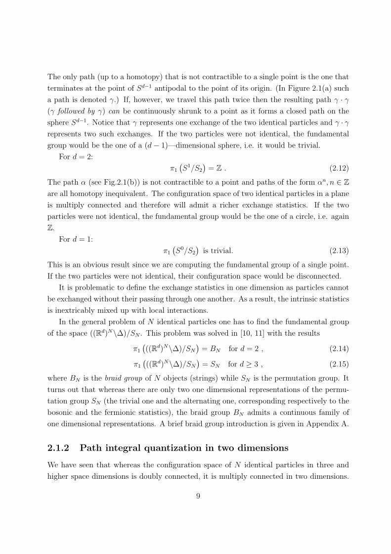
The relative coordinate R describes the motion around the guiding center. The corre-
sponding Heisenberg equations
dRx
dt=
1
i~[Rx, H] =
1
i~1
eB
1
2M[−Py, P
2x + P 2
y ] =1
MPx =
eB
MRy ,
dRy
dt= −eB
MRx (3.23)
are most easily solved if we notice that they are equivalent to a single equation
d
dt(Rx + iRy) = ωcRy − iωcRx = −iωc(Rx + iRy) , (3.24)
where
ωc =eB
M=
~M`2
B
(3.25)
is the cyclotron frequency. We can integrate (3.24),
(Rx + iRy)(t) = (R0x + iR0
y)e−iωct , (3.26)
i.e.
Rx(t) = R0x cos ωct + R0
y sin ωct ,
Ry(t) = R0y cos ωct−R0
x sin ωct , (3.27)
where R0x and R0
y are the integration constants. The relative coordinate R makes cyclotron
motion with the cyclotron frequency ωc.
It proves useful to introduce two pairs of operators
a ≡ `B√2~
(Px + iPy) , a† ≡ `B√2~
(Px − iPy)
b ≡ 1√2`B
(X − iY ) , b† ≡ 1√2`B
(X + iY ) , (3.28)
obeying
[a, a†
]=
[b, b†
]= 1 ,
[a, b] =[a†, b
]= 0 , (3.29)
which can be regarded as creation (a† and b†) and annihilation (a and b) operators of two
independent harmonic oscillators. We may define the Fock vacuum |0〉 by requiring
a|0〉 = 0 , b|0〉 = 0 (3.30)
23

and construct the Fock states upon it,
|N, n〉 =
√1
N !n!
(a†
)N (b†
)n |0〉 . (3.31)
In terms of the ladder operators a, a† the Hamiltonian (3.14) is rewritten as
H =1
2M(P 2
x + P 2y ) =
1
2M
((Px − iPy)(Px + iPy)− i[Px, Py]
)
=1
2M
(2~2
`2B
a†a +~2
`2B
)= ~ωc
(a†a +
1
2
). (3.32)
The energy levels, called the Landau levels, are found in the same way as for the
harmonic oscillator:
EN = ~ωc
(N +
1
2
)(3.33)
with the eigenstates |N, n〉,2 where n corresponds to the degeneracy within a Landau level.
A state |N, n〉 is called the Landau site and due to the Pauli exclusion principle it can
accommodate one electron in the spin-less theory and two electrons in the theory with
spins.
At this stage we choose the gauge, i.e. the electromagnetic potential Aext(x) such that
B = ∂yAextx − ∂xA
exty . We will work in the symmetric gauge
Aextx =
1
2By , Aext
y = −1
2Bx , (3.34)
in which the covariant momentum P and the guiding center X take the concrete form
Px = −i~∂
∂x+
eB
2y , Py = −i~
∂
∂y− eB
2x ,
X =1
2x− i~
eB
∂
∂y, Y =
1
2y +
i~eB
∂
∂x. (3.35)
The angular momentum operator (there is only one in a two dimensional system) is given
by
L ≡ −i~x∂
∂y+ i~y
∂
∂x=
eB
2(X2 + Y 2)− 1
2eB(P 2
x + P 2y ) = ~(b†b− a†a) . (3.36)
The states |N, n〉 are the eigenstates of L,
L|N,n〉 = ~(b†b− a†a)|N, n〉 = ~(n−N)|N, n〉 , (3.37)
2The quantum numbers N and n correspond, respectively, to the “oscillators” a and b.
24

with eigenvalues ~(n−N). Thus, b and b†, respectively, are the operators decreasing and
increasing the angular momentum of an electron.
We will now find the wave functions |N,n〉 explicitly. It is convenient to introduce a
pair of complex conjugate dimensionless coordinates
z =1
2`B
(x + iy) , z∗ =1
2`B
(x− iy) (3.38)
and the corresponding differential operators
∂
∂z= `B
(∂
∂x− i
∂
∂y
),
∂
∂z∗= `B
(∂
∂x+ i
∂
∂y
). (3.39)
The ladder operators (3.28) now take the form
a = − i√2
(z +
∂
∂z∗
), a† =
i√2
(z∗ − ∂
∂z
),
b =1√2
(z∗ +
∂
∂z
), b† =
1√2
(z − ∂
∂z∗
). (3.40)
In analogy with the harmonic oscillator, the states in the lowest Landau level (N = 0)
must satisfy
a|ψ〉 = 0 , i.e. − i√2
(z +
∂
∂z∗
)ψ(x) = 0 (3.41)
with the solution
ψ(x) = λ(z)e−zz∗ , (3.42)
where λ(z) is an arbitrary analytic function. The state |N = 0, n = 0〉 = |ψ0〉 has to
satisfy, in addition, the condition
b|ψ0〉 = 0 , i.e.1√2
(z∗ +
∂
∂z
)ψ0(x) = 0 . (3.43)
Since ψ0(x) = λ0(z)e−zz∗ , the latter reduces to
(z∗ +
∂
∂z
) (λ0(z)e−zz∗) =
∂λ0(z)
∂ze−zz∗ = 0 ⇒ λ0(z) = const . (3.44)
The normalization condition for |ψ0〉 dictates λ0(z) = (2π`2B)−1/2, so that
ψ0(x) =1√2π`2
B
e−|z|2
=1√2π`2
B
exp
(−x2 + y2
4`2B
). (3.45)
25
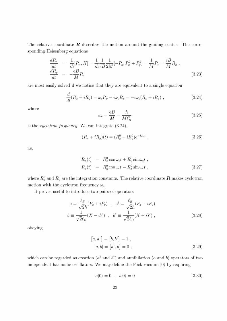
The states |ψn〉 = |0, n〉 from the lowest Landau level, but with higher angular momenta,
are obtained by repeated application of the b† operator on the vacuum |ψ0〉 (see (3.31)) —
ψn(x) =
√1
2nn!
(z − ∂
∂z∗
)n
ψ0(x) =
√2n
n!2π`2B
zne−|z|2
. (3.46)
In higher Landau levels the calculations get more complicated, leading to Laguerre poly-
nomials.
The probability that the electron in a state |ψn〉 is found at radius r = 2`B|z| is given
by
|ψn(x)|2 =2n
n!2π`2B
|z|2ne−2|z|2 ∝ r2n exp
(− r2
2`2B
), (3.47)
which has a sharp maximum at rn =√
2n`B. The area of a circle with radius rn is 2πn`2B.
It accommodates n Landau site (n possible values of the angular momentum), i.e. the area
of one Landau site is ∆S = 2π`2B. This holds for any Landau level, not only for the lowest
one.
For a sample of area S there are
S
∆S=
S
2π`2B
=e
2π~SB ≡ SB
ΦD
(3.48)
states in each Landau level. The constant ΦD = 2π~e
is the Dirac flux quantum. We define
the Landau level filling factor ν as the ratio between the total number of electrons in the
system and the number of states available in one Landau level:
ν :=ρ0SSBΦD
=ρ0ΦD
B, (3.49)
ρ0 is the electron density.
3.1.3 Many-particle states
It is straightforward to determine the ground state of the system at filling factor ν = 1,
i.e. when the lowest Landau level is completely filled. This is a particular case in the
integer QHE. For the wave function Ψ(x1, . . . , xN) of N electrons, where the appropriate
N depends on the size of the system as N = ρ0S = SBΨD
, the Pauli exclusion principle
implies that it is given by the Slater determinant constructed from the one particle wave
26

functions (3.46),
Ψ(x1, . . . , xN) =1√N !
∣∣∣∣∣∣∣∣∣∣
ψ0(x1) ψ1(x1) · · · ψN−1(x1)
ψ0(x2) ψ1(x2) · · · ψN−1(x2)...
...
ψ0(xN) ψ1(xN) · · · ψN−1(xN)
∣∣∣∣∣∣∣∣∣∣
∝
∣∣∣∣∣∣∣∣∣∣
1 z1 · · · zN−11
1 z2 · · · zN−12
......
1 zN · · · zN−1N
∣∣∣∣∣∣∣∣∣∣
e−∑N
j=1 |zj |2
=
(∏r<s
(zr − zs)
)e−
∑Nj=1 |zj |2 , (3.50)
where we have recognized the Vandermonde determinant.
In the case of fractional QHE, the Landau levels are not filled completely. The fractional
QH system develops a new type of collective ground state driven by the Coulomb repulsion
between the electrons that has been neglected so far, but now it becomes necessary to
explain the fractional QHE. A trial wave function of the ground state at filling factor
ν = 1m
, m odd, was first proposed by Laughlin [20],
Ψm(x1, . . . , xN) = Nm
(∏r<s
(zr − zs)m
)e−
∑Nj=1 |zj |2 , (3.51)
where Nm is the normalization factor.
Several properties of this wave function are to be pointed out. It is antisymmetric
under the exchange of any two electron positions. Since the prefactor∏
r<s(zr − zs)m is
purely analytic, all particles are in the lowest Landau level and since it is a polynomial in
z1, . . . , zN , Ψm is an eigenstate of the total angular momentum operator ~∑
r b†rbr. The
Coulomb repulsion among electrons is also contained in the prefactor, which has a zero of
order m at the points of coincidence zr = zs. The Laughlin wave function (3.51) is the
particular state, in which all electrons, having their own cyclotron motion, are repelled
from each other as much as possible. It is not an exact ground state, but it has a very
high overlap with numerical solutions for the QHE computed for various kinds of repulsive
potentials [20].
27

3.1.4 Quasiparticles in the fractional QHE
Quasiparticles in the FQHE are stable vortex solitons3 carrying fractional electric charges.
We shall see that they obey anyonic statistics, i.e. they are anyons. A quasihole is created
at the origin by transforming the polynomial part of the Laughlin wave function (3.51) as
follows
Ψ+m = N+
(∏
k
zk
∏r<s
(zr − zs)m
)e−
∑Nj=1 |zj |2 , (3.52)
[16] and [21]. This amounts to increasing the angular momentum of each electron by 1 and
pushing the electrons outwards from the vortex center. Similarly, a quasielectron is created
at the origin when the angular momentum of each particle decreases by 1 (and electrons
are pulled towards the vortex center),
Ψ−m = N−
(∏
k
∂
∂zk
∏r<s
(zr − zs)m
)e−
∑Nj=1 |zj |2 . (3.53)
The wave functions Ψ+m and Ψ−
m, being the eigenstates of the Hamiltonian as well as Ψm,
do not decay in time. The size of quasiparticles is of the order of `B (the magnetic length
(3.20)). Quasiholes are easier to analyze, but results analogous to those that will be derived
hold for quasielectrons as well.
The electric charge of a quasihole can be calculated using the concept of the Berry
phase4 [4]. The wave function describing a quasihole located at position zα is obtained
from (3.52) by the shift zk → zk − zα in the polynomial part,
Ψ+zαm = N+
α
(∏
k
(zk − zα)
)Ψm . (3.54)
3On the classical level, solitons are extended objects (classical field configurations) that are not de-formable continuously into a classical vacuum without violating the energy finiteness condition. One saysthat solitons are topologically stabilized.
4In quantum mechanics, the initial-state and final-state vectors of a cyclic evolution are related by aphase factor eiϕB (so called geometric or Berry phase), which can have observable consequences [22].
The concept of Berry phase was first published by M. V. Berry in 1984 [23] in the context of adiabaticevolution of a cyclic quantum system. Barry Simon explained the Berry phase mathematically as ananholonomy in the parameter space [24]. Later on, Y. Aharonov and J. Anandan showed that if theevolution is cyclic in the projective Hilbert space, the anholonomy is not based on the assumption ofadiabaticity [25]. Many further generalizations showed that the Berry phase is a pure artefact of thegeometry of the projective Hilbert space and hence is independent of the actual Hamiltonian (as long asthe curve in the projective Hilbert space is not changed).
28

Let us transport the quasihole adiabatically along a closed loop Γ so that zα becomes a
time-dependent parameter. Since the time dependence of Ψ+zαm (t) comes solely from zα(t),
we find thatd
dtΨ+zα
m (t) =∑
k
d ln(zk − zα(t))
dtΨ+zα
m (t) . (3.55)
The formula for calculating the Berry phase [25],
ϕB = i
∫ t1
t0
〈ψ(t)| ddt|ψ(t)〉 dt , (3.56)
takes the form
ϕB = i
∫ t1
t0
〈Ψ+zαm (t)|
∑
k
d ln(zk − zα(t))
dt|Ψ+zα
m (t)〉 dt , (3.57)
where the integral over t is evaluated from the time t0, when the quasihole begins its tour,
to the final time t1 when it returns to its original position. We will assume that the loop
Γ is traversed counterclockwise. (3.57) can be rewritten in terms of the electron density in
the state Ψ+zαm (t),
ρ(z) = 〈Ψ+zαm (t)|
∑
k
δ(2)(z − zk)|Ψ+zαm (t)〉 , (3.58)
so that
ϕB = i
∫ t1
t0
dt
∫d2z
d ln(z − zα(t))
dtρ(z)
= i
∫d2z
∫ t1
t0
dtdzα(t)
dt
ρ(z)
zα(t)− z
= i
∫d2z
∮
Γ
dzαρ(z)
zα − z. (3.59)
Under the reasonable assumption that the density ρ(z) is a regular function, only the points
z inside Γ will give non-vanishing contour integral∮
Γ1
zα−zdzα = 2πi. Thus
ϕB = i
∫
<Γ
d2z ρ(z)2πi = −2πNΓ , (3.60)
where the symbol∫
<Γd2z denotes the integral over the region inside Γ, and NΓ is the
number of electrons that are in there.
It can be shown [16] that the density of electrons in the state Ψ+zαm is uniform, i.e.
NΓ = ρ0SΓ, where SΓ is the area inside the loop Γ. Then NΓ can be related, using (3.49),
to the magnetic flux ΦΓ = −BSΓ penetrating the area enclosed by Γ,
NΓ = νBSΓ
ΦD
= −νΦΓ
ΦD
. (3.61)
29

If we identify the Berry phase with the Aharonov-Bohm phase ϕAB = ei~ qΦΓ (footnote ??)
that a particle of charge q acquires when it is moved along a closed loop encircling a flux
ΦΓ, we can deduce the unknown charge q:
ϕB = 2πνΦΓ
ΦD
=qΦΓ
~= ϕAB ⇒ q =
2π~ΦD
ν . (3.62)
Since by definition ΦD = 2π~e
and, in our case, the filling factor ν = 1m
, we obtain a bit
exotic result for the electric charge of a quasihole
eqh =e
m, (3.63)
where e is the elementary charge.
Analogously, one can derive [26] that the electric charge of a quasielectron is
eqe = − e
m. (3.64)
To find the exchange parameter α (2.20) between two quasiholes we utilize the wave
function
Ψ+zγ ,+zβm = N++
αβ
(∏
k
(zk − zγ)(zk − zβ)
)Ψm (3.65)
and calculate the Berry phase of an adiabatic process when the quasihole at zγ(t) is moved
along a closed loop Γ, while the quasihole at zβ is kept fixed. Along the same lines as when
we calculated the charge of a quasihole we arrive to
ϕB = i
∫ t1
t0
〈Ψ+zγ ,+zβm (t)| d
dt|Ψ+zγ ,+zβ
m (t)〉 dt = −2π
∫
<Γ
d2z ρ(z) , (3.66)
where ρ(z) is the electron density in the two-quasihole state,
ρ(z) = 〈Ψ+zγ ,+zβm (t)|
∑
k
δ(2)(z − zk)|Ψ+zγ ,+zβm (t)〉 . (3.67)
If zγ does not encircle zβ during its motion then ϕB = −2πNΓ. This corresponds to the
situation when the two quasiholes are not exchanged. On the other hand, if zβ is located
in the interior of Γ, the electron density inside Γ is no longer constant and the number of
electrons has to be diminished by 1m
. This yields the Berry phase
ϕB = −2π
(NΓ − 1
m
). (3.68)
The extra phase 2πm
, that accounts for one winding, i.e. two exchanges of the quasiholes, is
identified with 2α, where α is the anyonic exchange parameter. Therefore
α =π
m. (3.69)
We conclude that quasiholes in the fractional QHE at filling ν = 1m
, m = 3, 5, . . ., are
anyons with exchange phase ei πm .
30

3.1.5 Hall plateaux
So far we have studied the QH effect precisely at filling factor
ν =ρ0ΦD
B=
1
m. (3.70)
When the magnetic field B is increased by ∆B, the number of Landau sites (3.48) increases
by S∆BΦD
, i.e. the filling factor ν decreases. Each Landau site thus created accommodates
one quasihole. When B decreases by ∆B, the number of Landau sites decreases by S∆BΦD
,
ν increases and for each missing Landau site a quasielectron is created.
Since both electrons and quasiparticles are electrically charged, the Hall current is car-
ried by both of them and the Hall resistivity Rxy (3.4) is a linear function of B. But, this
is only true in pure samples. Real samples contain impurities that localize the quasipar-
ticles. In the vicinity of the magic filling factors ν = 1m
, only free electrons contribute to
the Hall current, which leads to the formation of Hall plateaux around ν = 1m
(Fig.3.3).
As the filling factor changes further, a Hall plateau is broken eventually since too many
quasiparticles are created to be localized by impurities.
Figure 3.3: Quasielectrons are excited for B > mρ0ΦD and quasiholes are excited for
B < mρ0ΦD. They are trapped by impurities and don’t contribute to the Hall current.
The Hall current remains unchanged in the vicinity of ν = 1m
, as is the origin on the Hall
plateau.
31

3.2 High-temperature superconductivity
Anyons gained a lot of attention when it was realized that they could provide a mech-
anism for the high-Tc superconductivity, observed in cuprate and other materials. The
current picture is that a gas of semions, i.e. anyons with the exchange parameter α = π2,
exhibits superfluidity and becomes superconducting if the anyons are electrically charged
[27]. However, it is an open question whether this mechanism can be observed experimen-
tally in nature.
As discussed in (2.27), anyons violate discrete symmetries of parity (P ) and time rever-
sal (T ). Therefore, by experience, their presence in a material should cause optical effects.
For example, linearly polarized light passing through sugar water rotates its direction of
polarization due to a definite handedness of the molecules in the solution. Another example
which breaks both (P ) and (T ) symmetries is the Faraday effect. In this effect, the direc-
tion of polarization of a linearly polarized light is rotated due to a magnetic field applied
to the sample in the direction of propagation. When the light is reflected and travels back
through the sample in the opposite direction, it does not “unrotate” its polarization axis
into the original state but rather rotates once again in the same direction (time reversal
violation).
It was suggested that the presence of anyons in the high-Tc materials should cause
effects similar to the Faraday effect. However, a careful experiment by Spielman et al.
[28] has found no signal of time reversal violation. It seems that anyons do not provide a
mechanism for the high-Tc superconductivity in the observed compounds (see [3], chapter
9 for more details). On the other hand, this does not rule out the possibility that anyonic
superconductors exist, but are yet to be discovered.
32
Chapter 4
Propagation of anyons on the toric
code
In quantum information theory, the toric code is a model that can serve as a platform
for quantum computational tasks. In particular, it can serve as a quantum memory — a
device that stores quantum information. The lifetime of such memory is the central issue
that decides about its potential practical usefulness. Excited states of the toric code are
interpreted as anyons. Under perturbations, these anyons can propagate and cause logical
errors. Our goal is to investigate the time evolution of the anyons living on the toric code
and to see whether a disorder imprinted in the system can guarantee their (Anderson)
localization.
4.1 Toric code – introduction
Quantum computer is a very powerful device. It can solve certain computational problems
qualitatively faster than an ordinary computer. For example, there is no published classical
algorithm decomposing efficiently an integer into its prime factors, yet a quantum algorithm
running on a quantum computer has been proposed by Peter Shor [29], which resolves this
problem in a time polynomial in the length of the input. Although there exist many
quantum algorithms that push the frontiers of what computers can manage to resolve,
the biggest challenge is the actual physical realization of a scalable and reliable quantum
computer. This is because real quantum systems are vulnerable to interaction with the
environment which causes decoherence of the quantum states, affects quantum information
and consequently discredits the outcome of the computation. Shor’s discovery of fault-
tolerant quantum computation [30] allowed the building blocks of a quantum circuit, the
33

quantum gates, to be imperfect, that is to be close to the ideal ones up to a constant
precision δ. Unfortunately, the threshold value of δ is very small (estimates vary) and thus
hard to achieve.
Classical gates are, in contrast, reliable enough, therefore classical computation doesn’t
need to be performed fault-tolerantly. Consider, for example, how classical information
is stored on a magnetic tape. Magnetism arises from spins of the individual atoms, each
of which is quite sensitive to thermal fluctuations. The spins tend to be oriented in the
same direction (to minimize the energy). If one spin is flipped to the opposite direction,
its interaction with the other spins forces it to flip back — errors are being corrected at
the physical level. In the quantum computational framework we can similarly propose a
quantum code with local stabilizer operators. Such code was invented by Alexei Kitaev in
1997 [5].
Consider an N ×N square lattice with “torus-like” identification (Fig.4.1). There are
Figure 4.1: Toric code is a square lattice wrapped around a torus. Spin-12
particles are
situated on each edge of the lattice and the stabilizer operators Av and Bp are defined,
respectively, for each vertex v and each plaquette p.
spin-12
particles located on each edge of the lattice. The total Hilbert space of this system
is
H = H⊗2N2
2 , (4.1)
34
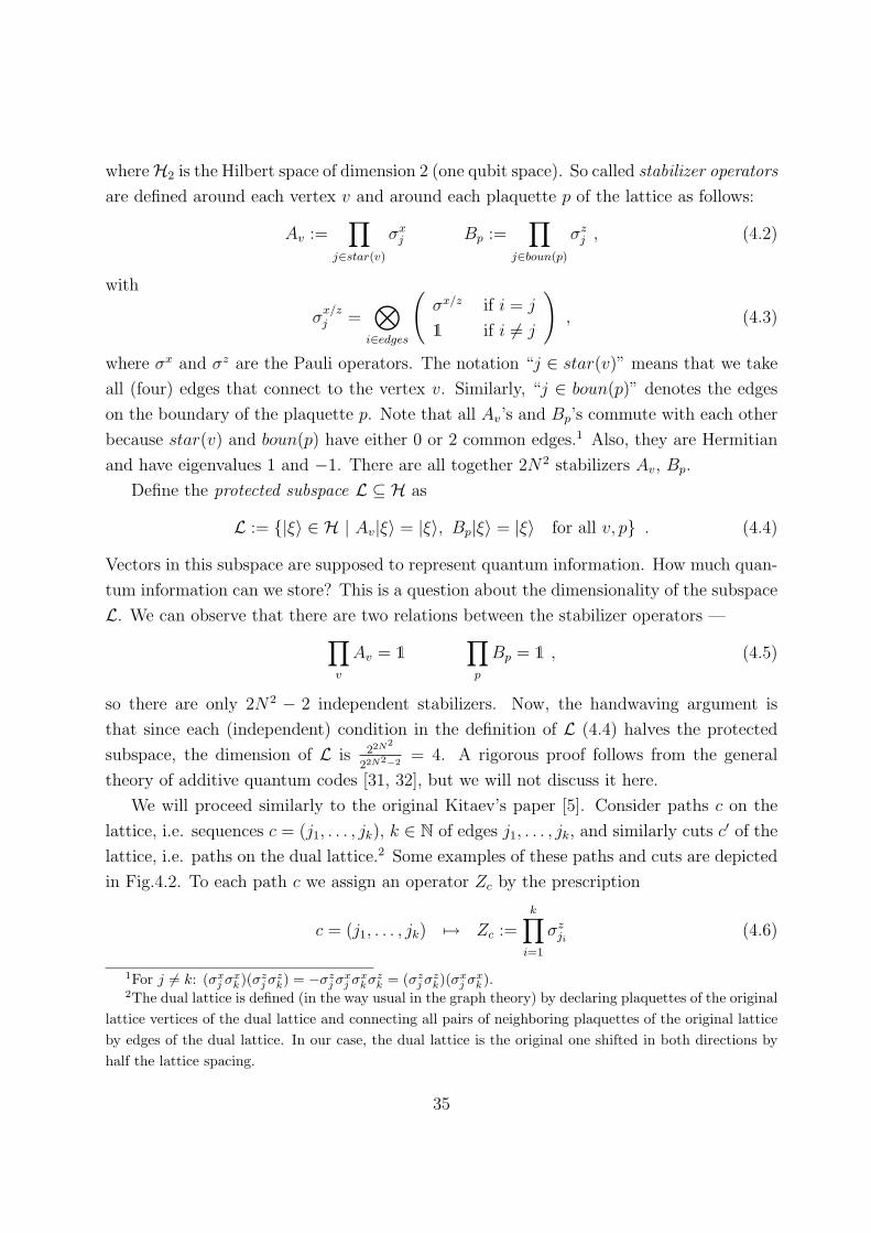
whereH2 is the Hilbert space of dimension 2 (one qubit space). So called stabilizer operators
are defined around each vertex v and around each plaquette p of the lattice as follows:
Av :=∏
j∈star(v)
σxj Bp :=
∏
j∈boun(p)
σzj , (4.2)
with
σx/zj =
⊗
i∈edges
(σx/z if i = j
1 if i 6= j
), (4.3)
where σx and σz are the Pauli operators. The notation “j ∈ star(v)” means that we take
all (four) edges that connect to the vertex v. Similarly, “j ∈ boun(p)” denotes the edges
on the boundary of the plaquette p. Note that all Av’s and Bp’s commute with each other
because star(v) and boun(p) have either 0 or 2 common edges.1 Also, they are Hermitian
and have eigenvalues 1 and −1. There are all together 2N2 stabilizers Av, Bp.
Define the protected subspace L ⊆ H as
L := |ξ〉 ∈ H | Av|ξ〉 = |ξ〉, Bp|ξ〉 = |ξ〉 for all v, p . (4.4)
Vectors in this subspace are supposed to represent quantum information. How much quan-
tum information can we store? This is a question about the dimensionality of the subspace
L. We can observe that there are two relations between the stabilizer operators —∏
v
Av = 1∏
p
Bp = 1 , (4.5)
so there are only 2N2 − 2 independent stabilizers. Now, the handwaving argument is
that since each (independent) condition in the definition of L (4.4) halves the protected
subspace, the dimension of L is 22N2
22N2−2= 4. A rigorous proof follows from the general
theory of additive quantum codes [31, 32], but we will not discuss it here.
We will proceed similarly to the original Kitaev’s paper [5]. Consider paths c on the
lattice, i.e. sequences c = (j1, . . . , jk), k ∈ N of edges j1, . . . , jk, and similarly cuts c′ of the
lattice, i.e. paths on the dual lattice.2 Some examples of these paths and cuts are depicted
in Fig.4.2. To each path c we assign an operator Zc by the prescription
c = (j1, . . . , jk) 7→ Zc :=k∏
i=1
σzji
(4.6)
1For j 6= k: (σxj σx
k)(σzj σz
k) = −σzj σx
j σxkσz
k = (σzj σz
k)(σxj σx
k).2The dual lattice is defined (in the way usual in the graph theory) by declaring plaquettes of the original
lattice vertices of the dual lattice and connecting all pairs of neighboring plaquettes of the original latticeby edges of the dual lattice. In our case, the dual lattice is the original one shifted in both directions byhalf the lattice spacing.
35

Figure 4.2: A generic path c on the lattice represents the operator Zc. Two topologically
nontrivial closed paths c1 and c2 define the operators Z1 and Z2 that act nontrivially on
the protected subspace L. Analogously, cuts c′ of the lattice, i.e. paths on the dual lattice,
represent the operators Xc′ . Two topologically nontrivial closed cuts c′1 and c′2 are shown
that define the operators X1 and X2. These operators act nontrivially on L.
and similarly to each cut c′ we assign Xc′ through
c′ = (j′1, . . . , j′k′) 7→ Xc′ :=
k′∏i=1
σxj′i
. (4.7)
We observe that if c (c′) is a closed loop then Zc (Xc′) commutes with all the stabilizers Av,
Bp and therefore is a mapping from L to L. We also observe that if a loop c is contractible,
i.e. if it is a boundary of some set of plaquettes P , the corresponding operator Zc acts on
L as the identity operator, Zc|ξ〉 = |ξ〉 for all |ξ〉 ∈ L, for it is a product of the stabilizers
Bp, p ∈ P . Similarly for the cuts c′. Thus, with respect to the protected subspace L, only
non-contractible loops and cuts are interesting.
On a torus we have two non-contractible loops (modulo the loops that are boundaries of
some region) — the first homology group has two generators. We denote these loops c1 and
c2 and the corresponding operators Z1 and Z2. Analogously, two non-contractible cuts c′1and c′2 define operators X1 and X2. The loops c1, c2 and the cuts c′1, c
′2 are drawn at Fig.4.2.
36

Realize that traveling any of these non-contractible loops or cuts twice yields the identity
operator so going to higher winding numbers is fruitless. The 4 operators Z1, Z2, X1, X2
have the same commutation relations as the operators (σz ⊗ 1), (1 ⊗ σz), (σx ⊗ 1), (1 ⊗σx). This is in agreement with the protected subspace being 4-dimensional, i.e. |ξ〉 ∈ Lcorresponding to a state of 2 qubits. The ground state of the toric code can encode 2 qubits
of quantum information. Hence, we may hope to use the toric code as quantum memory.
4.2 Toric code Hamiltonian and anyonic excitations
Consider the Hamiltonian
H0 = −∑
v∈vertices
Av −∑
p∈plaquettes
Bp . (4.8)
This Hamiltonian is more or less realistic, because it only involves local interactions —
each stabilizer acts only on four nearby spin-12
particles. It is easy to diagonalize as all
of the terms Av, Bp commute. The ground state subspace coincides with L; it is 4-fold
degenerate. Excited states occur if some of the constraints
Av|ξ〉 = |ξ〉 Bp|ξ〉 = |ξ〉 (4.9)
are violated. Since the eigenvalues of Av and Bp are ±1, the energy gap between the
ground state and any of the excited states is ∆E ≥ 2.
Let us construct an excited state by taking a string (a connected path) t, as pictured
in Fig.4.3(a), and applying the corresponding operator Zt (recall the definition (4.6)) to
some ground state |ξ〉. We obtain a state Zt|ξ〉 for which
Av1Zt|ξ〉 = −Zt|ξ〉 and Av2Zt|ξ〉 = −Zt|ξ〉 , (4.10)
where v1 and v2 are the two distinct endpoints of an open string t. We interpret this
violation the constraints (4.9) as two e-type particles occupying the vertices v1, v2. If t is
a closed string then Zt|ξ〉 ∈ L and no particles are created. Also note that for two strings
t1, t2 with common starting and ending points, Zt1|ξ〉 = Zt2|ξ〉 unless the loop “t1 followed
by t2” winds around the torus.
Analogously, with a cut t′ we have associated an operator Xt′ (definition (4.7)). If t′
has distinct endpoints p1, p2 (see Fig.4.3(a)) then
Bp1Xt′|ξ〉 = −Xt′|ξ〉 and Bp2Xt′|ξ〉 = −Xt′|ξ〉 , (4.11)
and we talk about two m-type particles occupying the plaquettes p1 and p2.
37

Figure 4.3: (a) A string t on the lattice represents the operator Zt. The endpoints of
t (vertices v1 and v2) are occupied by e-type particles. A string t′ on the dual lattice
represents the operator Xt′ . The endpoints of t′ (plaquettes p1 and p2) are occupied by
m-type particles. (b) The initial configuration described by the strings t and t′ presents a
pair of e particles and a pair of m particles. If one of the e particles moves around one of
the m particles (the cycle c), the global wave function acquires a phase factor −1. This
reveals anyonic statistics between the e and m-type particles.
4.2.1 Stability of a quantum memory
Suppose we initiate the toric code in a state |ξ〉 ∈ L. By doing so we have stored quantum
information. The question is: What will be the state of the system after some time? Will
it be |ξ〉 or will it change? How reliable is our quantum memory?
Errors might occur characterized by an operator
E =∏
j∈edges
(σxj )αj
∏
j∈edges
(σzj )
βj , αj, βj ∈ 0, 1 (4.12)
acting on the initial state |ξ〉. The new state E|ξ〉 is in general an excited state of the
Hamiltonian H0. It describes some configuration of e and m-type particles. The particles
represent elementary errors, violations of the stabilizer conditions (4.9). They always come
in pairs because of the relations (4.5).3 Due to the energy gap ∆E ≥ 2 between the ground
state and the excited levels, which remains finite in the thermodynamic limit, errors are
suppressed by coupling the toric code to a thermal bath with low temperature.
3Let, for instance, e particles be created at vertices from the set Ve = v | AvE|ξ〉 = −E|ξ〉. It holds
38

If the particles have been created, we can, in principle, bring them pairwise together to
perform error correction. This is realized by a correction operator C acting upon E|ξ〉 in
such a way that the operator CE contains only closed strings, so that the resulting state
CE|ξ〉 lies in the protected subspace L. If the error rate is below a certain threshold,4 the
error correction can be done through a minimum distance matching of the particle pairs
without forming topologically nontrivial loops. The resulting state CE|ξ〉 will be equal to
the initial state |ξ〉, i.e. the quantum information will remain unchanged. If, however, the
error rate is too high, we can’t avoid creating topologically nontrivial loops (such as the
operators Z1, Z2, X1, X2). The state CE|ξ〉 might then be different from |ξ〉, which results
in a logical error — the information stored in the quantum memory is changed.
4.2.2 Anyonic statistics revealed
Consider a perturbation to the toric code Hamiltonian H0 (definition 4.8) of the form
V = −hx
∑
j∈edges
σxj − hz
∑
j∈edges
σzj , (4.13)
where the constants hx and hz measure the strength of the perturbation. This perturbation
does not commute with the original Hamiltonian H0. The eigenstates of H0 are therefore
no longer eigenstates of the perturbed Hamiltonian H = H0 + V . As a consequence, e and
m particles will propagate rather then stay at their initial positions.
What happens if the particles move around each other? Consider the initial state
|Ψi〉 = Xt′Zt|ξ〉 , |ξ〉 ∈ L (4.14)
pictured in Fig.4.3(b), which describes a configuration of two e particles and two m parti-
cles. Let, for example, one of the e particles move around one of the m particles and end
up at its initial position. The state of the system is now described by the wave function
|Ψf〉 = ZcXt′Zt|ξ〉 = −Xt′ZtZc|ξ〉 = −|Ψi〉 , (4.15)
that
E|ξ〉 =
(∏v
Av
)E|ξ〉 =
( ∏
v∈Ve
Av
) ∏
v 6∈Ve
Av
E|ξ〉 =
( ∏
v∈Ve
Av
)E|ξ〉 = (−1)|Ve|E|ξ〉 ,
where |Ve| denotes the number of elements of the set Ve.4If P denotes the probability of an individual σx error, the threshold is estimated as P ≈ 0.11 [33].
The same holds for σz errors.
39

because the operators Xt′ and Zc anti-commute. We can see that the global wave function
acquires a phase factor −1. The e and m-type particles are quite different from bosons
and fermions, which do not change sign in such a process. Indeed, they are (Abelian)
anyons and we will call them e anyons and m anyons from now on. Notice that the
anyonic statistics is revealed only between e and m particles, not between e (or m) particles
themselves. In terms of the Aharonov-Bohm effect interpretation (footnote 5) we can
view the e anyons as electric charges and m anyons as magnetic fluxes with appropriate
combination (charge) × (flux) = π so that the Aharonov-Bohm phase ei(charge)×(flux) is
equal to −1.
The effect of the perturbation (4.13), which would be caused by a spurious magnetic
field in any physical realization of the toric code, is to create, annihilate and transport!
anyons. If this acts unchecked, even a single pair of anyons can form a topologically
nontrivial loop around the torus, thus causing a logical error (a final state |ξf〉 ∈ L that
is different from the initial state |ξi〉 ∈ L). Therefore, to know how stable our quantum
memory is, we need to investigate the propagation of errors, i.e. the anyons, on the toric
code lattice. If they exhibit some sort of localization (at least under certain assumptions),
the toric code will get one step closer to become a reliable quantum memory.
4.2.3 Perturbation induced anyonic quantum walks
Let us first make clear that the unperturbed Hamiltonian H0 defined in (4.8) doesn’t
induce any motion of the anyonic excitations. Choose an orthonormal basis of L: L =
span|ξ−−〉, |ξ−+〉, |ξ+−〉, |ξ++〉, where
Z1|ξs1s2〉 = s1|ξs1s2〉 , Z2|ξs1s2〉 = s2|ξs1s2〉 . (4.16)
Take two arbitrary configurations of anyons described by two sets of strings — the operators
Z(i)t X
(i)t′ and Z
(f)t X
(f)t′ — acting on some ground state |ξs1s2〉 ≡ |ξ〉. We observe that the two
states |i〉 = Z(i)t X
(i)t′ |ξ〉 and |f〉 = Z
(f)t X
(f)t′ |ξ〉 are orthogonal, 〈f |i〉 = 0, if they correspond
to two different configurations of anyons, since in that case |i〉 and |f〉 are two distinct
eigenvectors of some Hermitian operator Av or Bp. Also, 〈f |i〉 = 0 if |i〉 and |f〉 describe
the same anyonic configuration, but distinct logical states. Therefore, the matrix elements
〈f |H0|i〉 = −∑
v
〈f |Av|i〉 −∑
p
〈f |Bp|i〉 = −∑
v
±〈f |i〉 −∑
p
±〈f |i〉 (4.17)
can be nonzero only for |i〉, |f〉 describing identical anyonic configurations and logical
states, i.e. H0 is diagonal in the basis of anyonic configurations. The time evolution of a
40

state |i〉 is then trivial, only multiplying |i〉 by the phase factor eiEi , i.e. the anyons don’t
move around.
Introducing a perturbation V as in (4.13) makes the anyons walk. We put hx = 0 for
simplicity and hz ≡ h for brevity. Now, the Hamiltonian of the system
H = H0 + V = −∑
v∈vert
Av −∑
p∈plaq
Bp − h∑
j∈edges
σzj (4.18)
leaves the m-type anyons static since for any configuration |i〉 and any plaquette p
Bp|i〉 = sp|i〉 , sp ∈ −, + ⇒ Bp(H|i〉) = HBp|i〉 = sp(H|i〉) . (4.19)
On the other hand, H induces a nontrivial evolution of the e anyons — a continuous-time
quantum walk. To see this, realize that H has nonzero off-diagonal matrix elements. Given
two states |i〉 = Z(i)t X
(i)t′ |ξ〉 and |f〉 = Z
(f)t X
(f)t′ |ξ〉 we observe that
〈f |(−V )|i〉 = h∑
j∈edges
〈ξ|X(f)t′ Z
(f)t σz
j Z(i)t X
(i)t′ |ξ〉 = h〈ξ|X(f)
t′ Z(f)t σz
j Z(i)t X
(i)t′ |ξ〉
= ±h〈ξ|Z(f)t σz
j Z(i)t X
(f)t′ X
(i)t′ |ξ〉 = ±h〈ξ|ξ〉 = ±h (4.20)
if for some edge j, Z(f)t σz
j Z(i)t forms a system of closed loops only and X
(i)t′ , X
(f)t′ corre-
spond to identical configuration of the m anyons. To determine the ± sign one needs to
calculate how many times the Pauli operators σx and σz are transposed when going from
X(f)t′ Z
(f)t σz
j Z(i)t X
(i)t′ to the expression Z
(f)t σz
j Z(i)t X
(f)t′ X
(i)t′ . For this purpose we recall the
discussion related to Fig.4.3(b). The ± depends on how many m anyons in the X(f)t′ con-
figuration are enclosed by the loops Z(f)t σz
j Z(i)t with “+” corresponding to an even number
and “−” to an odd number of anyons. The result only depends on the positions of the m
anyons and not on the particular way they are connected by the strings X(f)t′ .
Our goal is to investigate how the e anyons will propagate under the action of the
evolution operator e−itH , given some fixed (random) configuration of the m anyons. In this
context we would like to mention the Wootton’s and Pachos’ paper [7] where the authors
consider a perturbed toric code Hamiltonian
HTC + Hh = −∑
v
JvAv −∑
p
JpBp − h∑
j
σzj . (4.21)
and analyze the propagation of the e anyons with no m anyons present in the system.
They show that if Jv’s are not uniform but take random values on each vertex and h ¿ Jv,
the disorder in the system can successfully localize the anyons by placing an exponential
41

bound on the length of their propagation. Their arguments are based on the theory of
Anderson localization (see the original Anderson’s paper [6] or a recent overview [34]).
In our case the Jv’s are uniform and for our choice of units Jv = 1. The random
property of our system is the m anyon configuration. Does this kind of randomness lead to
a localization of the e anyons as in [7] or does it not? To make the analysis more tractable
we will investigate a simplified topological model. Instead of a torus we will define our
code on a strip with one periodic identification. The lattice will resemble a ladder and we
will refer to it as the ladder lattice.
4.3 Ladder lattice model
In analogy with the toric code, we define a stabilizer code on a ladder-like lattice with one
identification depicted in Figure 4.4. There are N vertices in the horizontal direction and
Figure 4.4: The stabilizer code defined on a square lattice on a strip — a ladder with one
identification. Spin-12
particles are situated on each edge of the lattice and the stabilizer
operators Av and Bp are defined for each vertex v and plaquette p, respectively (in analogy
with the original toric code, Fig.4.1).
2 vertices in the vertical direction. Spin-12
particles live on the edges of the lattice, the
stabilizer operators Av consist of three Pauli operators σx surrounding a vertex v,
Av :=∏
j∈star(v)
σxj , (4.22)
and the stabilizer operators Bp form the boundary of a plaquette p,
Bp :=∏
j∈boun(p)
σzj . (4.23)
The protected subspace L ⊆ H contains vectors |ξ〉 such that
Av|ξ〉 = |ξ〉 , Bp|ξ〉 = |ξ〉 (4.24)
42

for all vertices v and plaquettes p. The subspace L has dimension 2. Corresponding to
this code is the unperturbed Hamiltonian
H0 = −∑
v∈vertices
Av −∑
p∈plaquettes
Bp , (4.25)
the lowest energy eigenspace of which coincides with L. An e-type anyon occurs on a
vertex v whenever
Av|ψ〉 = −|ψ〉 (4.26)
and similarly an m-type anyon occurs on a plaquette p for which
Bp|ψ〉 = −|ψ〉 . (4.27)
Anyons of both types are created in pairs and they occupy the endpoints of a string of σz
operators (for the e anyons) and the endpoints of a cut of σx operators (for the m anyons).
We introduce a perturbation to H0 of the form V = −h∑
j σzj . The full Hamiltonian
now reads
H = −∑
v∈vertices
Av −∑
p∈plaquettes
Bp − h∑
j∈edges
σzj (4.28)
and it induces a quantum walk of the e anyons while keeping the m anyons static. The
logical error occurs when one e anyon from a pair propagates all the way around the ladder
and annihilates with its fellow e anyon. During this process a loop Z of σz matrices is
formed which maps the logical state |ξ〉 into another logical state Z|ξ〉, causing a logical
error. Our goal is to probe how the e anyons will propagate in a static pattern of the m
anyons. What effect will the nontrivial braiding properties of the anyons (recall Fig.4.3)
have on their quantum walk?
We assume that the perturbation V is weak (h ¿ 1). Then the e anyon pairs are
created sparsely and each pair can be considered independently. We will thus analyze a
single pair only. Creation and annihilation of a pair of anyons is energetically suppressed
by the energy gap ∆E = 2.
Let us introduce some notation as suggested by Fig.4.5. We denote H the Hilbert space
of one e anyon configurations, i.e.
H = span|x, y〉 ≡ |x〉 ⊗ |y〉 | x = 1, . . . , N , y = 0, 1 (4.29)
is the space of all positions (vertices) one e anyon can occupy. Let
M = m1, . . . ,m|M | ⊆ 1, . . . , N (4.30)
43

Figure 4.5: Vertices of the ladder are denoted by a pair x = 1, . . . , N (the horizontal axis)
and y = 0, 1 (the vertical axis). Each vertex corresponds to one basis vector of the one-
e-anyon Hilbert space H. There are N plaquettes numbered by integers 1, . . . , N . The
identification on the two sides of the ladder is illustrated.
denote the set of plaquettes where m anyons are located. For a logical state |ξ〉 ∈ L we
denote |ξM〉 the state of |M | anyons of type m that have been created upon |ξ〉 and moved
to plaquettes from the set M = m1, . . . , m|M |.5Once |ξM〉 has been fixed and a pair of e anyons created we represent configurations of
the two e anyons by the vectors |x1, y1〉 ⊗ |x2, y2〉 ∈ H ×H.6 To establish the connection
with the original Hilbert space of the code (which is fully analogous to (4.1)) we need
to choose a canonical manner in which the string Zt connecting the two e anyons is laid
down.7 For this purpose choose and fix a point (x0, 0) on the ladder. Let (x1, y1) and
(x2, y2) be the positions of the two e anyons. The canonical string Zt1 starts at (x0, 0),
connects straightly and by the shortest way to the vertex (x1, 0) and then to the vertex
(x1, y1). Accordingly, Zt2 connects sequentially (x0, 0), (x2, 0) and (x2, y2). The canonical
string between the two positions (x1, y1) and (x2, y2) is the composition Zt = Zt1Zt2 (see
Fig.4.6).
5More precisely,|ξM 〉 = Xt′ |ξ〉 ,
where Xt′ is a collection of strings of σx operators whose endpoints are m1, . . . ,m|M |. The set M carriesno information about a concrete layout of the strings. This information, however, is not important forthe braiding properties of the anyons, which is what we want to probe. It is only important how many m
anyons an e anyon encircles during its travel (see Fig.4.3 in this context).6Strictly speaking, since the e anyons are indistinguishable, we should represent them by symmetrized
vectors |x1, y1〉⊗ |x2, y2〉+ |x2, y2〉⊗ |x1, y1〉. We will not be as punctual, because in a while we will reduceour problem to a one particle walk only.
7Keep in mind that Zt1 |ξM 〉 and Zt2 |ξM 〉 are the same quantum state (they differ only by a phasefactor) if Zc = Zt1Zt2 is a closed contractible loop.
44
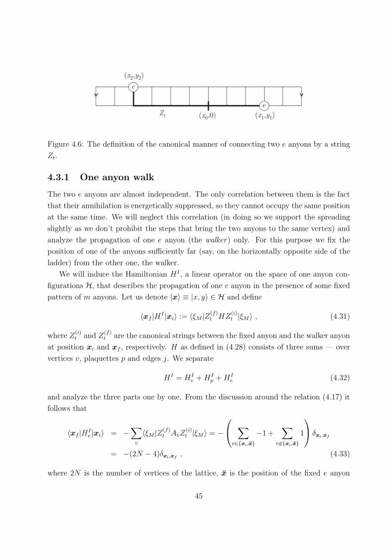
Figure 4.6: The definition of the canonical manner of connecting two e anyons by a string
Zt.
4.3.1 One anyon walk
The two e anyons are almost independent. The only correlation between them is the fact
that their annihilation is energetically suppressed, so they cannot occupy the same position
at the same time. We will neglect this correlation (in doing so we support the spreading
slightly as we don’t prohibit the steps that bring the two anyons to the same vertex) and
analyze the propagation of one e anyon (the walker) only. For this purpose we fix the
position of one of the anyons sufficiently far (say, on the horizontally opposite side of the
ladder) from the other one, the walker.
We will induce the Hamiltonian HI , a linear operator on the space of one anyon con-
figurations H, that describes the propagation of one e anyon in the presence of some fixed
pattern of m anyons. Let us denote |x〉 ≡ |x, y〉 ∈ H and define
〈xf |HI |xi〉 := 〈ξM |Z(f)t HZ
(i)t |ξM〉 , (4.31)
where Z(i)t and Z
(f)t are the canonical strings between the fixed anyon and the walker anyon
at position xi and xf , respectively. H as defined in (4.28) consists of three sums — over
vertices v, plaquettes p and edges j. We separate
HI = HIv + HI
p + HIe (4.32)
and analyze the three parts one by one. From the discussion around the relation (4.17) it
follows that
〈xf |HIv |xi〉 = −
∑v
〈ξM |Z(f)t AvZ
(i)t |ξM〉 = −
∑
v∈xi,x−1 +
∑
v 6∈xi,x1
δxi,xf
= −(2N − 4)δxi,xf, (4.33)
where 2N is the number of vertices of the lattice, x is the position of the fixed e anyon
45

and δxi,xf= 1 if xi = xf and δxi,xf
= 0 otherwise. Similarly,
〈xf |HIp |xi〉 = −
∑p
〈ξM |Z(f)t BpZ
(i)t |ξM〉 = −
(∑p∈M
−1 +∑
p6∈M
1
)δxi,xf
= −(N − 2|M |)δxi,xf. (4.34)
The case of He is a bit more subtle, but it results from the relation (4.20) and the discussion
that follows it:
〈xf |HIe |xi〉 = −h
∑j
〈ξM |Z(f)t σz
j Z(i)t |ξM〉 = −hδ〈xi,xf 〉s(xi,xf ) , (4.35)
where δ〈xi,xf 〉 = 1 if the vertex xi neighbors with xf and δ〈xi,xf 〉 = 0 otherwise. The factor
s(xi,xf ) accounts for the nontrivial braiding properties between e and m-type anoyns:
s(xi, xf ) =
−1 if yi = yf = 1 and min(xi, xf ) ∈ M
1 otherwise .(4.36)
It is illustrated at Figure 4.7. The expression (4.35) is incorrect for vertices xi, xf located
Figure 4.7: The factor s(xi,xf ) = −1 in the case depicted due to the nontrivial braiding
properties between e and m-type anyons (recall Fig.4.3).
horizontally opposite of (x0, 0) since then topologically nontrivial loops can be formed.
We will neglect this fact as it does not affect our point — whether the particle remains
localized around (x0, 0) or spreads. Otherwise we would have to restrict ourselves to a
certain neighborhood of (x0, 0) with boundaries which would make our analysis much more
technical.
The time evolution of the system is governed by the evolution operator U I(t) = eitHI.
Since HIv and HI
p are just multiples of the identity operator, U I(t) factorizes as8
U I(t) = eit(HIv+HI
p+HIe ) = eitHI
v eitHIp eitHI
e . (4.37)
8We use the fact that eA+B = eAeB if the commutator [A,B] = 0.
46

The operator eitHIv eitHI
p = e−it(2N−4)e−it(N−2|M |)1 only multiplies the wave function by a
global phase factor and as such is irrelevant. The propagation, or quantum walk, of one e
anyon is described by the Hamiltonian HIe . In the position basis |x〉 the matrix − 1
hHI
e
has entries ±1 and it is convenient and illuminating to represent it by a graph with edge
weights ±1. This graph coincides with the ladder lattice graph and it is depicted in Fig.4.8.
Algebraically, the operator HIe : H → H reads
Figure 4.8: The adjacency matrix of this weighted graph is − 1hHI
e . The weight is −1 for an
edge that is the upper boundary of a plaquette containing an m anyon and it is 1 otherwise.
HIe = −h (1⊗H2 + H0 ⊗ |0〉〈0|+ H~ε ⊗ |1〉〈1|) , (4.38)
where
H2 = |0〉〈1|+ |1〉〈0| , (4.39)
H0 =N∑
x=1
(|x + 1〉〈x|+ |x〉〈x + 1|) , (4.40)
H~ε =N∑
x=1
εx (|x + 1〉〈x|+ |x〉〈x + 1|) (4.41)
and where the dependency on the set M is realized through a vector ~ε = (ε1, . . . , εN)
defined by
εx =
−1 if x ∈ M
1 if x 6∈ M .(4.42)
In the above formulae, the identification |N + 1〉 ≡ |1〉 is implied.
Our goal now is to determine the transition amplitudes 〈x|eitHIe |x0〉 that carry the full
information about the walker’s propagation. From the transition amplitudes we can de-
rive the time evolution of the position distribution |〈x|eitHIe |x0〉|2, from which we can tell
whether the particle spreads around the lattice and causes a logical error or remains local-
ized. In the next section we will analyze in detail one dimensional problems (continuous-
time quantum walks) defined by the Hamiltonians H0 and H~ε.
47

4.4 Continuous-time quantum walks in one dimension
We will analyze the quantum evolution of a particle living on a one dimensional lattice.
In literature, especially in the quantum information theory, this problem is called the
continuous-time quantum walk [35]. Indeed, it is inspired by the classical random walk
and translates it into the quantum mechanical framework.
While the time we take continuous, the space is considered discrete. This can be
thought of as a tight binding approximation — the particle is anchored to a vertex by a
sufficiently deep and thin potential well.
4.4.1 Cyclic lattice
Let us consider a free spinless quantum particle moving on a cycle graph with N vertices
(Fig.4.9). The Hilbert space of this system is N -dimensional,
Figure 4.9: The particle moves on a one dimensional periodic lattice pictured as a cycle
graph with N vertices. The hopping amplitudes for all neighboring sites are all equal to 1
(there is no disorder).
H = span|x〉Nx=1 , (4.43)
where |x〉 are the normalized eigenvectors of the position operator, X|x〉 = x|x〉. We
impose periodic boundary conditions |x = N + 1〉 = |x = 1〉 and |x = 0〉 = |x = N〉 and
consider the Hamiltonian
H = −N∑
x=1
(|x + 1〉〈x|+ |x〉〈x + 1|) , (4.44)
48
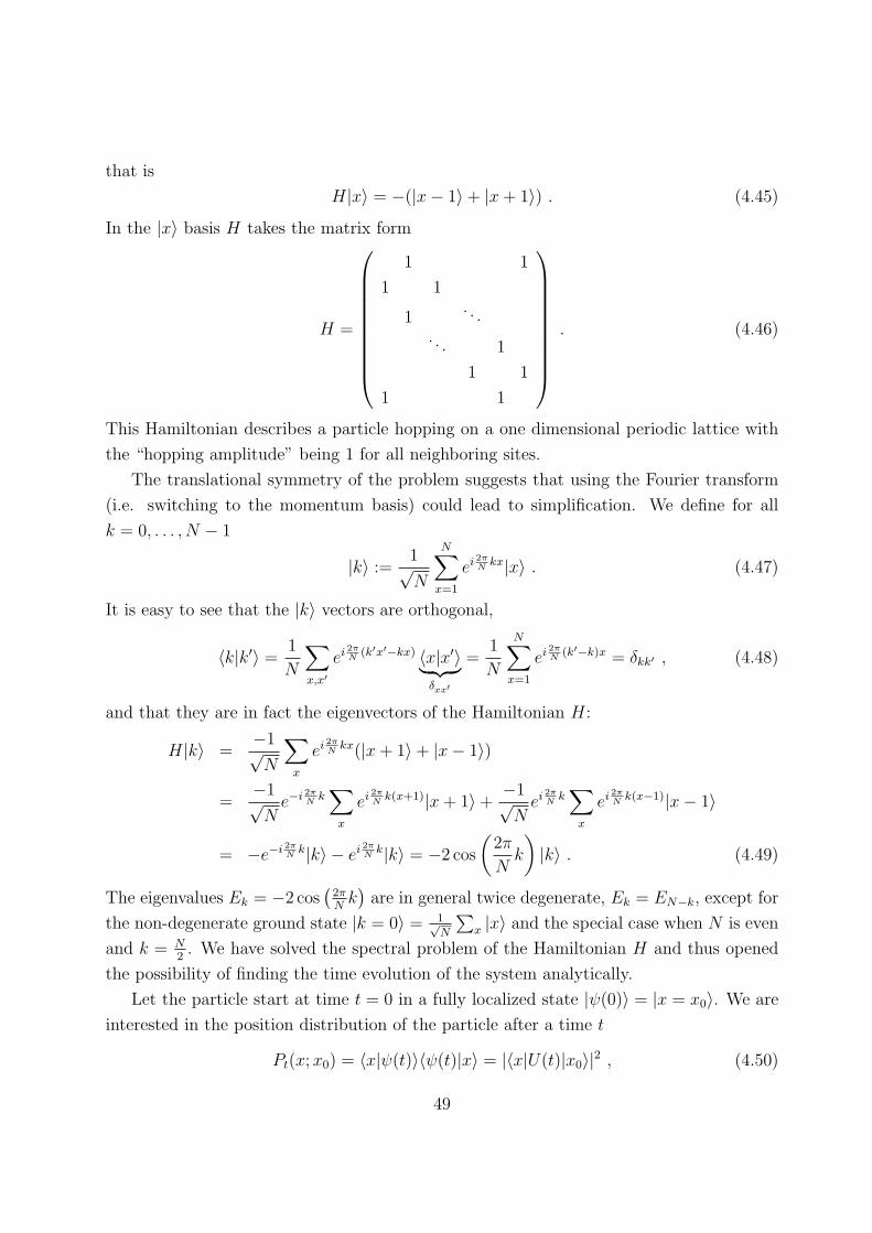
that is
H|x〉 = −(|x− 1〉+ |x + 1〉) . (4.45)
In the |x〉 basis H takes the matrix form
H =
1 1
1 1
1. . .
. . . 1
1 1
1 1
. (4.46)
This Hamiltonian describes a particle hopping on a one dimensional periodic lattice with
the “hopping amplitude” being 1 for all neighboring sites.
The translational symmetry of the problem suggests that using the Fourier transform
(i.e. switching to the momentum basis) could lead to simplification. We define for all
k = 0, . . . , N − 1
|k〉 :=1√N
N∑x=1
ei 2πN
kx|x〉 . (4.47)
It is easy to see that the |k〉 vectors are orthogonal,
〈k|k′〉 =1
N
∑
x,x′ei 2π
N(k′x′−kx) 〈x|x′〉︸ ︷︷ ︸
δxx′
=1
N
N∑x=1
ei 2πN
(k′−k)x = δkk′ , (4.48)
and that they are in fact the eigenvectors of the Hamiltonian H:
H|k〉 =−1√N
∑x
ei 2πN
kx(|x + 1〉+ |x− 1〉)
=−1√N
e−i 2πN
k∑
x
ei 2πN
k(x+1)|x + 1〉+−1√N
ei 2πN
k∑
x
ei 2πN
k(x−1)|x− 1〉
= −e−i 2πN
k|k〉 − ei 2πN
k|k〉 = −2 cos
(2π
Nk
)|k〉 . (4.49)
The eigenvalues Ek = −2 cos(
2πN
k)
are in general twice degenerate, Ek = EN−k, except for
the non-degenerate ground state |k = 0〉 = 1√N
∑x |x〉 and the special case when N is even
and k = N2. We have solved the spectral problem of the Hamiltonian H and thus opened
the possibility of finding the time evolution of the system analytically.
Let the particle start at time t = 0 in a fully localized state |ψ(0)〉 = |x = x0〉. We are
interested in the position distribution of the particle after a time t
Pt(x; x0) = 〈x|ψ(t)〉〈ψ(t)|x〉 = |〈x|U(t)|x0〉|2 , (4.50)
49

where |ψ(t)〉 = U(t)|ψ(0)〉 and U(t) = e−itH is the evolution operator. For this sake we
calculate the amplitude of transition from the state |x0〉 to the state |x〉 in time t using
the resolution of unity in terms of the eigenvectors of H — 1 =∑N−1
k=0 |k〉〈k|. We obtain
〈x|U(t)|x0〉 = 〈x|e−itH |x0〉 =∑
k
e−itEk〈x|k〉〈k|x0〉
=1
N
N−1∑
k=0
ei2t cos( 2πN
k)ei 2πN
k(x−x0) . (4.51)
We can now plug these transition amplitudes into (4.50) to find the position distribution
Pt(x; x0). The result is plotted at Fig.4.12 for N = 200, x0 = 100 and times t = 20, 50.
The particle is spread around the cycle when t is large enough.
We can derive (4.51) using a rather different approach — without diagonalizing the
Hamiltonian. Starting with
〈x|U(t)|x0〉 = 〈x|e−itH |x0〉 (4.52)
and expanding the exponential,
〈x|e−itH |x0〉 =∞∑
n=0
(it)n
n!〈x|(−H)n|x0〉 , (4.53)
we realize that the terms 〈x|(−H)n|x0〉 answer a classical question: How many ways can a
classical particle (a drunken sailor) walking on a cycle graph with N vertices get in n-steps
from the point x0 to the point x. Due to the periodicity of the cycle we have
〈x|(−H)n|x0〉 =∑
p∈Z
(n
x+pN−x0
2+ n
2
), (4.54)
where we use the usual convention that(
nk
)= 0 if k 6∈ 0, 1, . . . , n. We rewrite the latter
in terms of the Kronecker δ symbol,
〈x|(−H)n|x0〉 =∑
p∈Z
n∑j=0
(n
j
)δ2j,x+pN−x0+n =
n∑j=0
(n
j
) ∑
p∈Zδ2j,x+pN−x0+n (4.55)
and use the relation
1
N
N−1∑
k=0
ei 2πN
k(r−s) =
1 if r = s + pN for some p ∈ Z0 otherwise
(4.56)
50

to obtain
〈x|(−H)n|x0〉 =n∑
j=0
(n
j
)1
N
N−1∑
k=0
ei 2πN
k(x−x0+n−2j)
=1
N
N−1∑
k=0
ei 2πN
k(x−x0)
n∑j=0
(n
j
)ei 2π
Nk(n−j)e−i 2π
Nkj
=1
N
N−1∑
k=0
ei 2πN
k(x−x0)(ei 2π
Nk + e−i 2π
Nk)n
=1
N
N−1∑
k=0
ei 2πN
k(x−x0)
(2 cos
2π
Nk
)n
. (4.57)
Plugging this back into (4.53), the transition amplitudes read
〈x|U(t)|x0〉 =∞∑
n=0
(it)n
n!〈x|(−H)n|x0〉
=1
N
N−1∑
k=0
ei 2πN
k(x−x0)ei2t cos( 2πN
k) , (4.58)
which, indeed, equals (4.51).
4.4.2 Infinite line
What happens if we send N → ∞? This corresponds to replacing a finite circle by an
infinite line.9 The sum in (4.51) is replaced by an integral, kN
by z and 1N
by dz. The
transition amplitudes read
〈x|U(t)|x0〉|N→∞ =
∫ 1
0
ei2t cos(2πz)ei2πz(x−x0)dz =1
2π
∫ 2π
0
ei2t cos zeiz(x−x0)dz , (4.59)
where now x0, x ∈ Z. After the substitution z → −z + π2
and using the fact that the
integrated function is 2π-periodic,
1
2π
∫ 2π
0
ei2t cos zeiz(x−x0)dz =ix−x0
2π
∫ 2π
0
ei2t sin ze−iz(x−x0)dz (4.60)
and we unveil the integral representation of the Bessel functions of the first kind ([36],
formula 8.411.1). This gives the transition amplitudes a compact form
〈x|U(t)|x0〉|N→∞ = ix−x0Jx−x0(2t) . (4.61)
9It is important that we carry out the limit N →∞ at the beginning and not only work in a large (butfinite) N regime, where our following conclusions would be valid merely for x − x0 and t small enoughcompare to N .
51

The position distribution of the particle in the N →∞ limit then takes the form
Pt(x; x0)|N→∞ = |〈x|U(t)|x0〉|2N→∞ = (Jx−x0(2t))2 . (4.62)
It is plotted in Figure 4.10(a).
Figure 4.10: (a) The position distribution Pt(x; 0)|N→∞ of a particle walking on the infinite
line graph, initially localized at position x0 = 0, is shown for the time interval t ∈ [0, 15]
and the sites x ∈ 0, . . . , 20 (Pt(x; 0)|N→∞ is symmetric with respect to x0). (b) The
variance of the distribution Pt(x; 0)|N→∞ grows quadratically with t.
Let us put x0 = 0 for simplicity. The moments of the probability distribution Pt(x; 0)|N→∞,
〈Xm〉(t) =∞∑
x=−∞xm (Jx(2t))
2 , (4.63)
can be expressed in the following way. For the Bessel J function it holds that
e±i2t sin z =∞∑
x=−∞Jx(2t)e
±ixz (4.64)
52

([36], formula 8.511.4). We may write
〈Xm〉(t) =∞∑
x=−∞
∞∑
x′=−∞xmJx(2t)Jx′(2t)
1
2π
∫ 2π
0
e−ix′zeixzdz
︸ ︷︷ ︸δx,x′
=∞∑
x=−∞
∞∑
x′=−∞Jx(2t)Jx′(2t)
1
2π
∫ 2π
0
e−ix′z(−i)m ∂m
∂zmeixzdz
=1
2π
∫ 2π
0
( ∞∑
x′=−∞Jx′(2t)e
−ix′z
)(−i)m ∂m
∂zm
( ∞∑x=−∞
Jx(2t)eixz
)dz (4.65)
and using (4.64) we derive
〈Xm〉(t) =(−i)m
2π
∫ 2π
0
e−i2t sin z ∂m
∂zmei2t sin zdz . (4.66)
It is not difficult to calculate first few moments explicitly:
〈X0〉(t) = 1 (4.67)
reflects a proper normalization of the probability distribution;
〈X1〉(t) = 0 (4.68)
is the mean value (generally, 〈X1〉(t) = x0);
〈X2〉(t) = 2t2 (4.69)
is in our case equal to the variance 〈X2〉 − 〈X〉2, which measures the spreading (or delo-
calization) of the particle (Fig.4.10(b));
〈X3〉(t) = 0 , (4.70)
〈X4〉(t) = 2t2(1 + 3t2) , etc . . . (4.71)
In general, 〈X2m+1〉(t) = 0 for all m ∈ N since Pt(x; 0)|N→∞ is an even function of x.10
An explicit calculation of the even moments 〈X2m〉(t), m ∈ N, requires to perform
repeated differentiation of a composite function. However, we can easily (with the aid of
[36], formula 3.621.3) find at least the leading term of 〈X2m〉(t) for arbitrary m:
〈X2m〉(t) =(−i)2m
2π
∫ 2π
0
(i2t)2m(cos z)2mdz + . . . (lower orders of t)
=
(2m
m
)t2m + . . . . (4.72)
10It holds thatJ−n(t) = (−1)nJn(t)
for n ∈ Z.
53

4.4.3 Cyclic lattice with disordered couplings
We can generalize the previous model by allowing the “hopping amplitudes” for neighboring
sites to take values +1 or −1 (Fig.4.11). We hence get a family of Hamiltonians
Figure 4.11: The particle moves on a one dimensional periodic lattice with N sites. The
hopping amplitudes are allowed to take values εj = ±1, j = 1, . . . , N .
H~ε = −N∑
x=1
εx (|x + 1〉〈x|+ |x〉〈x + 1|) , (4.73)
or
H~ε|x〉 = −(εx−1|x− 1〉+ εx|x + 1〉) , (4.74)
characterized by binary vectors
~ε = (ε1, ε2, . . . , εN) , εj ∈ −1, 1 . (4.75)
The boundary conditions are again periodic, |x = N +1〉 = |x = 1〉 and |x = 0〉 = |x = N〉,and we define ε0 := εN . Note that the undisordered Hamiltonian (4.44) is contained in
this family as the special case ~ε = (1, . . . , 1) ≡ ~1.
We shall see that the generalized problem is solvable for any configuration ~ε. Well, let
us try to solve the spectral problem for H~ε,
H~ε|ψ〉 = E|ψ〉 , (4.76)
which leads to the set of N equations
−εx−1〈x− 1|ψ〉 − εx〈x + 1|ψ〉 = E〈x|ψ〉 , x = 1, . . . , N (4.77)
54

for the components of |ψ〉 in the X-representation. We may regard this as a linear recur-
rence relation for a finite sequence 〈x|ψ〉N+1x=0 subject to the boundary conditions
〈0|ψ〉 = 〈N |ψ〉〈N + 1|ψ〉 = 〈1|ψ〉 . (4.78)
After multiplying (4.77) by∏N
j=x εj and rearranging the terms we face (keep in mind that
ε2x = 1 for all x)
(N∏
j=x+1
εj
)〈x+1|ψ〉+E
(N∏
j=x
εj
)〈x|ψ〉+
(N∏
j=x−1
εj
)〈x−1|ψ〉 = 0 , x = 1, . . . , N . (4.79)
Now, for ~ε = ~1 we know that the Hamiltonian is the one without disorder and its
eigenvectors are given by (4.47). Fortunately, we can get rid of the ~ε dependence in the
recurrence (4.79) by making the ansatz
〈x|ψ〉 =
(N∏
j=x
εj
)ei 2π
Nωx , x = 0, . . . , N + 1 . (4.80)
(We use the usual convention∏b
j=a(. . .) = 1 if a > b.) One can easily convince oneself that
such |ψ〉 satisfies the equations (4.79) provided that
E = −2 cos
(2π
Nω
). (4.81)
The parameter ω is restricted by the boundary conditions (4.78) that for our choice of |ψ〉read
(N∏
j=0
εj
)= εNei2πω (4.82)
ei 2πN
ω(N+1) =
(N∏
j=1
εj
)ei 2π
Nω . (4.83)
Since, by definition, ε0 = εN , these two conditions are equivalent and yield
ei2πω = sgn(~ε) , (4.84)
where we denoted
sgn(~ε) ≡N∏
j=1
εj = ±1 . (4.85)
55

If sgn(~ε) = +1,
ω = k , k = 0, . . . , N − 1 . (4.86)
The eigenvalues of H~ε are
E+k = −2 cos
(2π
Nk
), k = 0, . . . , N − 1 (4.87)
and the (orthonormal) eigenvectors of H~ε read
|k+ε〉 =1√N
N∑x=1
(N∏
j=x
εj
)ei 2π
Nkx|x〉 , k = 0, . . . , N − 1 . (4.88)
If sgn(~ε) = −1,
ω = k +1
2, k = 0, . . . , N − 1 . (4.89)
The eigenvalues of H~ε are
E−k = −2 cos
(2π
Nk +
π
N
), k = 0, . . . , N − 1 (4.90)
and the (orthonormal) eigenvectors of H~ε read
|k−ε〉 =1√N
N∑x=1
(N∏
j=x
εj
)ei π
Nxei 2π
Nkx|x〉 , k = 0, . . . , N − 1 . (4.91)
Let’s check the orthonormality of the vectors |k+ε〉:
〈k+ε1 |k+ε
2 〉 =1
N
∑x1,x2
(N∏
j=x1
εj
)(N∏
j=x2
εj
)e−i 2π
Nk1x1ei 2π
Nk2x2〈x1|x2〉 (4.92)
=1
N
∑x1
ei 2πN
(k2−k1)x1 = δk1,k2 . (4.93)
In the same way we can prove the orthonormality of the vectors |k−ε〉.Once the eigenvectors are known, it is easy to probe the time evolution of the system.
Depending on sgn(~ε), the transition amplitudes are either
〈x|U+ε(t)|x0〉 = 〈x|e−itH~ε|x0〉 =∑
k
e−itE+εk 〈x|k+ε〉〈k+ε|x0〉
=1
N
(N∏
j=x
εj
)(N∏
j=x0
εj
)N∑
k=1
ei2t cos( 2πN
k)ei 2πN
k(x−x0) (4.94)
56

for sgn(~ε) = +1, or
〈x|U−ε(t)|x0〉 = 〈x|e−itH~ε|x0〉 =∑
k
e−itE−εk 〈x|k−ε〉〈k−ε|x0〉
=1
N
(N∏
j=x
εj
)(N∏
j=x0
εj
)ei π
N(x−x0)
N∑
k=1
ei2t cos( 2πN
k+ πN )ei 2π
Nk(x−x0) (4.95)
for sgn(~ε) = −1. To obtain the position distribution after time t, starting with a localized
state |ψ(0)〉 = |x0〉, we calculate the modulus squared of the transition amplitudes (4.94)
and (4.95). Clearly, the results only depend on sgn(~ε), not on the details εj of the particular
configuration ~ε:
P+t (x; x0) =
1
N2
∣∣∣∣∣N∑
k=1
ei2t cos( 2πN
k)ei 2πN
k(x−x0)
∣∣∣∣∣
2
for sgn(~ε) = +1 ,
P−t (x; x0) =
1
N2
∣∣∣∣∣N∑
k=1
ei2t cos( 2πN
k+ πN )ei 2π
Nk(x−x0)
∣∣∣∣∣
2
for sgn(~ε) = −1 . (4.96)
The position distributions P+t (x; x0) and P+
t (x; x0) are plotted at Fig.4.12 and Fig.4.13,
respectively, for the cycle of length N = 200, the initial state |x0〉 = |100〉, and times t =
20, 50. The particle (initially fully localized) spreads around the cycle, i.e. its localization
is lost. This holds for both sgn(~ε) = +1 and −1 and the corresponding plots are in fact
hardly told apart by eye.
Remark: Yet, it can be important whether we have ~ε such that sgn(~ε) = +1 or −1.
Consider two simple examples of cycles of size N = 4 with the hopping amplitudes as
pictured in Fig.4.14. Let us choose the initial state |x0〉 = |1〉 and calculate the particle’s
distribution after a time t. For each site |x〉 we obtain a function of t, P±t (x; x0). The results
for (a) sgn(~ε) = +1 and (b) sgn(~ε) = −1 are plotted at Fig.4.15(a) and (b), respectively.
The interference phenomena change dramatically the propagation of the particle. In
particular, in the case (b) the particle can never (for no t) be found at the opposite corner
of the square (position |x = 3〉). This is because the particle’s histories traveling from |1〉to |3〉 via |2〉 pick up phases opposite to those traveling via |4〉.
4.5 Numerical results for one anyon walk on a peri-
odic ladder lattice
We have seen in the previous section that a particle living on a one dimensional lattice
with nearest neighbour interaction tends to spread for any choice of disorder ~ε in the
57
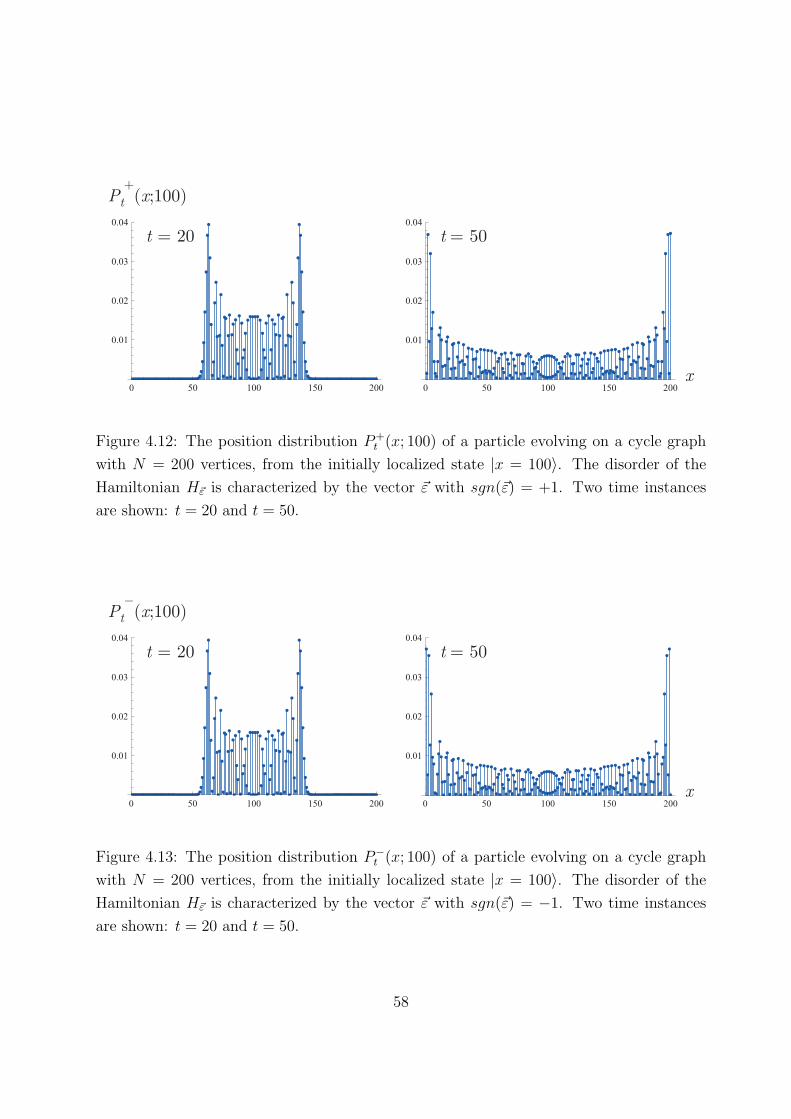
Figure 4.12: The position distribution P+t (x; 100) of a particle evolving on a cycle graph
with N = 200 vertices, from the initially localized state |x = 100〉. The disorder of the
Hamiltonian H~ε is characterized by the vector ~ε with sgn(~ε) = +1. Two time instances
are shown: t = 20 and t = 50.
Figure 4.13: The position distribution P−t (x; 100) of a particle evolving on a cycle graph
with N = 200 vertices, from the initially localized state |x = 100〉. The disorder of the
Hamiltonian H~ε is characterized by the vector ~ε with sgn(~ε) = −1. Two time instances
are shown: t = 20 and t = 50.
58

Figure 4.14: (a) A lattice corresponding to ~ε = (1, 1, 1, 1), sgn(~ε) = +1. (b) A lattice with
hopping amplitudes corresponding to ~ε = (1, 1,−1, 1), sgn(~ε) = −1. The initial state is
|x0〉 = |1〉.
Figure 4.15: The probabilities of finding a particle initiated at vertex |1〉 on a square lattice
(see Fig.4.14) are plotted as functions of time t for various sites |x〉. (a) The case when
sgn(~ε) = +1. (b) The case when sgn(~ε) = −1. The two cases differ most significantly at
the site |3〉.
Hamiltonian H~ε (4.73), specially for the Hamiltonian H0 (4.44). For an infinite lattice,
the variance of the resulting position distribution grows as ∼ t2 (4.69). In the finite case,
when N is the number of sites of the periodic lattice, this quadratic dependence holds until
the spreading wave function starts to interfere with itself as the two parts propagating in
opposite directions meet and mix together.
We have also seen that the presence of −1 hopping terms in the Hamiltonian causes
59

destructive interference (recall Fig.4.15) that can play an important role for small cycles,
where the wave function mixes almost immediately.
For the periodic ladder lattice (4.8) these two attributes coexist. Since for a general
configuration of the m anyons we are unable to diagonalize the corresponding Hamiltonian
(4.38) analytically, we turn to numerics.
4.5.1 Regular disorder – delocalization
Let us first consider the case of regularly placed m anyons. Suppose there is an m anyon
on every second plaquette. The Hamiltonian HIe , which we will denote simply H from now
on, is of the form
H ≡ HIe = −h (1⊗H2 + H0 ⊗ |0〉〈0|+ H~ε ⊗ |1〉〈1|) (4.97)
with
εx =
1 if x is odd
−1 if x is even .(4.98)
We choose a localized initial state |ψ0〉 = |x0〉 ⊗ |0〉 and calculate |ψ(t)〉 = U(t)|ψ0〉 —
the wave function after a time t. To find U(t) = e−itH , it is necessary to diagonalize the
Hamiltonian H, i.e. to find a diagonal matrix A and a transformation matrix S such that
H = SAS−1. This step is done numerically. We are interested in the position distribution
along the horizontal axis of the ladder
P regt (x; x0) =
1∑y=0
〈x, y|ψ(t)〉〈ψ(t)|x, y〉 = |〈x, 0|U(t)|ψ0〉|2 + |〈x, 1|U(t)|ψ0〉|2 . (4.99)
From P regt (x; x0) we calculate the corresponding variance
V arreg(t) =N∑
x=1
x2P regt (x; x0)−
(N∑
x=1
xP regt (x; x0)
)2
(4.100)
that tells us quantitatively about the spreading of the particle.
The time scale is defined by the perturbation strength h (~ = 1 from the very begin-
ning). It is convenient to introduce the dimensionless time
τ := ht . (4.101)
The numerical results are presented for the ladder horizontal size N = 200, the initial
position x0 = 100 and for τ ∈ [0, 200] with time-step ∆τ = 1. Figure 4.16 shows the
60

Figure 4.16: The position distributions P regt (x; 100) are shown for τ = 20, 50, 100, 200. The
particle, initially localized around x0 = 100, fills up the ladder about the time τ = 100.
position distributions P regt (x; 100) for τ = 20, 50, 100, 200, Figure 4.17 illustrates how the
variance V arreg changes with time. At τ = 100 the variance reaches its maximum
value V arreg = 3128.14. This is comparable to the variance of the uniform distribution
P uni(x) = 1N
, which comes out as
V aruni =1
N
N∑x=1
x2 −(
1
N
N∑x=1
x
)2
=N2 − 1
12= 3333.25 . (4.102)
The walker, clearly, gets delocalized — logical error is likely to occur at τ = 100 = N2.
4.5.2 Random disorder – localization
More realistically, m errors occur at random positions, they don’t form a regular pattern.
We will consider a model in which an m anyon occupies a given plaquette with probability
61

Figure 4.17: The variance of the walker’s position distribution for regularly placed m
anyons, V arreg, as a function of the dimensionless time τ grows as ∼ τ 2 up to the point
(τ = 100, V arreg = 3128.14) when oppositely propagating parts of the wave function |ψ(t)〉meet.
12. This probability is equal for all plaquettes.11 That is, on average there should be one
half of the plaquettes populated. The pattern, however, is random and this fact proves to
be fundamental for the motion of the e anyonic walker.
We are interested in the quantities averaged over all configurations (patterns) M ⊆1, . . . , N of the m anyons (see (4.30)). N denotes the number of plaquettes as usually.
There are 2N possible configurations and all of them are realized with the equal probability1
2N . Let us start with a localized initial state |ψ0〉 = |x0〉⊗ |0〉. The M -averaged horizontal
position distribution of the walker after a time t reads
P rant (x; x0) =
1
2N
∑
M⊆1,...,N
(∣∣〈x, 0|UM(t)|ψ0〉∣∣2 +
∣∣〈x, 1|UM(t)|ψ0〉∣∣2
), (4.103)
where UM(t) is the evolution operator corresponding to the Hamiltonian HIe (4.73) with
the disorder ~ε specified by the particular set M ,
εx =
−1 if x ∈ M
1 if x 6∈ M .(4.104)
The M -averaged variance V arran(t) is calculated from P rant (x; x0) in a standard way,
V arran(t) =N∑
x=1
x2P rant (x; x0)−
(N∑
x=1
xP rant (x; x0)
)2
. (4.105)
11This yields a rather dense (and perhaps unrealistic) population of the m anyons. We want to distillthe effect of a random pattern even when the lattice that we are able to probe numerically is rather small.We believe that the effects would be similar for large lattices and sparsely distributed m anyons.
62
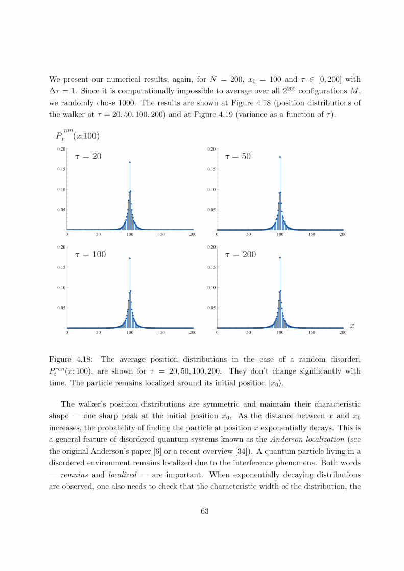
We present our numerical results, again, for N = 200, x0 = 100 and τ ∈ [0, 200] with
∆τ = 1. Since it is computationally impossible to average over all 2200 configurations M ,
we randomly chose 1000. The results are shown at Figure 4.18 (position distributions of
the walker at τ = 20, 50, 100, 200) and at Figure 4.19 (variance as a function of τ).
Figure 4.18: The average position distributions in the case of a random disorder,
P rant (x; 100), are shown for τ = 20, 50, 100, 200. They don’t change significantly with
time. The particle remains localized around its initial position |x0〉.
The walker’s position distributions are symmetric and maintain their characteristic
shape — one sharp peak at the initial position x0. As the distance between x and x0
increases, the probability of finding the particle at position x exponentially decays. This is
a general feature of disordered quantum systems known as the Anderson localization (see
the original Anderson’s paper [6] or a recent overview [34]). A quantum particle living in a
disordered environment remains localized due to the interference phenomena. Both words
— remains and localized — are important. When exponentially decaying distributions
are observed, one also needs to check that the characteristic width of the distribution, the
63

Figure 4.19: The variance of the walker’s position distribution for randomly placed m
anyons, V arran, as a function of the dimensionless time τ grows slowly and is much smaller
than the variance V arreg in the case of the regular disorder (Fig.4.17).
localization length, does not grow with time ad infinitum.
Figure 4.20 shows that our position distributions P rant (x; x0) can be fit to a decaying
exponential reasonably well; the localization length being 3.5 at τ = 200. The time de-
pendence of the width of the position distribution can be read off from Fig.4.19, i.e. from
the time evolution of the variance, which grows slowly of perhaps even stops growing.
Although our numerical results show only the time range τ ∈ [0, 200] and are of limited
accuracy, they support strongly our final conclusion: An e anyon living on a ladder-like
lattice in a random environment of static m anyons remains localized, it’s motion is expo-
nentially suppressed. As a consequence, the logical errors of the corresponding quantum
memory are also exponentially suppressed — the time it takes for a logical error to occur
is exponentially large in the size of the system.
64

Figure 4.20: The position distributions P rant (x; 100) can be fit to a decaying exponential.
We show the fit for the “right wing” of the distribution at τ = 200. The fit is e−x−x03.5 up
to a constant prefactor. The localization length is 3.5 in this case.
65

Chapter 5
Conclusion
We have reviewed the theory (Chapter 2) as well as the experimental aspects (Chapter 3)
of two dimensional particles with exotic exchange statistics called anyons.
In the last chapter we investigated the propagation of anyons on the toric code to inspect
the stability of this topological quantum memory. We used a simplified model defined on
a strip with a ladder-like lattice. The evolution of a quantum particle (a continuous-time
quantum walk) was exactly solved in one dimension for a finite cycle (4.51), an infinite
line (4.61) and a finite cycle with disordered couplings between the neighboring vertices
(4.94, 4.95) (they were allowed to take values +1 or −1). We showed that any disorder of
the type under consideration leads to the same delocalization behavior as in the case of
uniform coupling. Subsequently, we studied numerically the propagation of an anyon on
the ladder lattice with disorder and compared two cases. When the disorder was regular,
periodic, the particle delocalized (Fig.4.16 and 4.17). On the other hand, in the case of a
random disorder, the Anderson localization effect took place and the anyon remained at its
initial position (Fig.4.18 and 4.19). More precisely, its wave function decayed exponentially
with the distance.
Hence, we have shown (in analogy with [7]) that a random disorder imprinted in a
topological quantum memory can be used to improve its robustness against logical errors.
66

Appendix A
Braid group
Braids are formed when n points on a horizontal plane are connected by n strands to
n points on another horizontal plane, parallel to the first one, directly below the first n
points. The strings are not allowed to go back upwards at any point in their travel. Two
braids are considered the same (or equivalent) if one can be transformed into the other via
an ambient isotopy of the space (a continuous deformation that doesn’t cross the strings)
that fixes the endpoints of each string (Fig.A.1).
Figure A.1: An example of equivalent braids. One can be transformed into the other via
an ambient isotopy of the space that fixes the endpoints of each string.
In order to describe a given braid we define the braid group. The braid group Bn of
n-strand braids is a group generated by n− 1 symbols σ1, ..., σn−1 (depicted in Fig.A.2(a))
with the operation of concatenation (Fig.A.2(b)). The identity element is the diagram
with “n straight lines” (Fig.A.3(a)) and the inverse of a generator σj, denoted σ−1j , has the
type of crossing opposite from σj (Fig.A.3(b)).
The generators of the braid group satisfy two additional relations:
σiσi+1σi = σi+1σiσi+1 for i ∈ 1, 2, ..., n− 2 , (A.1)
σiσj = σjσi for i, j ∈ 1, ..., n− 1, |i− j| ≥ 2 . (A.2)
67

Figure A.2: (a) The generators σj of the braid group Bn (j runs from 1 to n− 1). (b) The
braid group operation of concatenation — one braid is put on top of the other and the
corresponding strands are glued together.
Figure A.3: (a) The identity element in the braid group Bn. (b) The inverses of the
generators σj of Bn.
These relations are pictured in Figure A.4. The group relation σ−1j σj = σjσ
−1j = 1 together
with the relations (A.1) and (A.2) guarantee that any two words in braid generators (and
their inverses) represent the same braid if and only if they are the same element of Bn.
These three relations correspond to the three Reidemeister moves — the three knot pre-
serving transformations (for an introduction into the knot theory see e.g. [37]). This group
approach to braids is due to Emil Artin [38] and therefore Bn is sometimes called the Artin
braid group.
Physical relevance of the braid group is apparent from the following observation. Con-
sider n indistinguishable particles in a plane (Fig.A.5), which we will identify with the
complex plane C, and assume two particles cannot occupy the same position. The config-
68

Figure A.4: The braid group relations: (a) represents the relation A.1 and (b) represents
the relation A.2. The braid on the left hand side is the same as that on the right hand
side.
Figure A.5: Four indistinguishable particles in a plane evolving in time. As the particles
move around one another, their worldlines in the 2+1 dimensional spacetime constitute a
braid (provided that the initial and the final configuration is the same). The braid group
B4 is the fundamental group of the space of four indistinguishable particles.
uration space of this physical system is
X = (Cn\∆)/Sn , (A.3)
where ∆ = (z1, ..., zn) ∈ Cn | zi = zj for some i 6= j and Sn is the permutation group
of n symbols. As the particles move around in the plane, their worldlines trace curves
in the 2 + 1 dimensional spacetime as depicted in Figure A.5. One can prove a plausible
statement that the braid group Bn is the fundamental group of the space X, i.e.
Bn = π1(X). (A.4)
69

A.1 Representations of the braid group
One-dimensional unitary representations of the braid group Bn are easy to classify. Let
us assign complex numbers eiαj , αj ∈ [0, 2π], to the generators σj. The relation (A.2) is
clearly satisfied. The other braid group relation (A.1) translates into
eiαjeiαj+1eiαj = eiαj+1eiαjeiαj+1 for j ∈ 1, 2, ..., n− 2 , (A.5)
which enforces eiα1 = . . . = eiαn−1 ≡ eiα. The angle α is the only parameter characterizing
the particular representation
ρα : σj 7→ eiα , j ∈ 1, 2, ..., n− 1 . (A.6)
We can see that the representation ρα is not faithful as it does not distinguish distinct
braid group elements σjσj+1 and σj+1σj. On the other hand, unlike the symmetric group
Sn, ρα does tell apart the identity and the elements σ2j (provided that α 6= 0, π). In fact,
Sn differs from Bn only by the additional requirement σ2j = 1, which allows only two
one-dimensional unitary representations ρ+ : σj 7→ 1 and ρ− : σj 7→ −1.
The braid group representation theory in higher dimensions is much richer and much
more complicated. It is connected with the polynomial invariants of knots. An interested
reader is directed to [39] for an overview.
70

Bibliography
[1] J. Leinaas and J. Myrheim, “On the theory of identical particles,” Il Nuovo Cimento
B (1971-1996), vol. 37, pp. 1–23, 1977. 10.1007/BF02727953.
[2] F. D. M. Haldane, ““fractional statistics” in arbitrary dimensions: A generalization
of the pauli principle,” Phys. Rev. Lett., vol. 67, pp. 937–940, Aug 1991.
[3] A. Khare, Fractional statistics and quantum theory. World Scientific, 2005.
[4] D. Arovas, J. R. Schrieffer, and F. Wilczek, “Fractional statistics and the quantum
hall effect,” Phys. Rev. Lett., vol. 53, pp. 722–723, Aug 1984.
[5] A. Y. Kitaev, “Fault-tolerant quantum computation by anyons,” Annals of Physics,
vol. 303, no. 1, pp. 2 – 30, 2003.
[6] P. W. Anderson, “Absence of diffusion in certain random lattices,” Phys. Rev., vol. 109,
pp. 1492–1505, Mar 1958.
[7] J. R. Wootton and J. K. Pachos, “Bringing order through disorder: Localisation of
errors in topological quantum memories,” ArXiv e-prints, Jan. 2011.
[8] R. Mirman, “Experimental meaning of the concept of identical particles,” Il Nuovo
Cimento B (1971-1996), vol. 18, pp. 110–122, 1973. 10.1007/BF02832643.
[9] W. Massey, A basic course in algebraic topology. Graduate texts in mathematics,
Springer-Verlag, 1991.
[10] R. Fox and L. Neuwirth, “The braid groups,” Mathematica Scandinavia, vol. 10, p. 119,
1962.
[11] E. Fadell and L. Neuwirth, “Configuration spaces,” Mathematica Scandinavia, vol. 10,
p. 111, 1962.
71

[12] R. Feynman and A. Hibbs, Quantum mechanics and path integrals [by] R. P. Feynman
[and] A. R. Hibbs. International series in pure and applied physics, McGraw-Hill, 1965.
[13] M. G. G. Laidlaw and C. M. DeWitt, “Feynman functional integrals for systems of
indistinguishable particles,” Phys. Rev. D, vol. 3, pp. 1375–1378, Mar 1971.
[14] W. Pauli, “The connection between spin and statistics,” Phys. Rev., vol. 58, pp. 716–
722, Oct 1940.
[15] Y. Aharonov and D. Bohm, “Significance of electromagnetic potentials in the quantum
theory,” Phys. Rev., vol. 115, pp. 485–491, Aug 1959.
[16] Z. Ezawa, Quantum Hall effects: field theoretical approach and related topics. World
Scientific, 2008.
[17] K. v. Klitzing, G. Dorda, and M. Pepper, “New method for high-accuracy determi-
nation of the fine-structure constant based on quantized hall resistance,” Phys. Rev.
Lett., vol. 45, pp. 494–497, Aug 1980.
[18] E. H. Hall, “On a new action of the magnet on electric currents,” American Journal
of Mathematics, vol. 2, no. 3, pp. 287 – 292, 1879.
[19] D. C. Tsui, H. L. Stormer, and A. C. Gossard, “Two-dimensional magnetotransport
in the extreme quantum limit,” Phys. Rev. Lett., vol. 48, pp. 1559–1562, May 1982.
[20] R. B. Laughlin, “Anomalous quantum hall effect: An incompressible quantum fluid
with fractionally charged excitations,” Phys. Rev. Lett., vol. 50, pp. 1395–1398, May
1983.
[21] A. Stern, “Anyons and the quantum hall effect–a pedagogical review,” Annals of
Physics, vol. 323, no. 1, pp. 204 – 249, 2008. January Special Issue 2008.
[22] A. Bohm, A. Mostafazadeh, H. Koizumi, Q. Niu, and J. Zwanziger, The Geometric
Phase in Quantum Systems: Foundations, Mathematical Concepts, and Applications
in Molecular and Condensed Matter Physics. Theoretical and Mathematical Physics
Series, Springer, 2010.
[23] M. V. Berry, “Quantal phase factors accompanying adiabatic changes,” Proceedings
of the Royal Society of London. A. Mathematical and Physical Sciences, vol. 392,
no. 1802, pp. 45–57, 1984.
72

[24] B. Simon, “Holonomy, the quantum adiabatic theorem, and berry’s phase,” Phys.
Rev. Lett., vol. 51, pp. 2167–2170, Dec 1983.
[25] Y. Aharonov and J. Anandan, “Phase change during a cyclic quantum evolution,”
Phys. Rev. Lett., vol. 58, pp. 1593–1596, Apr 1987.
[26] A. Lerda, Anyons: quantum mechanics of particles with fractional statistics. Lecture
notes in physics: Monographs, Springer-Verlag, 1992.
[27] F. Wilczek, Fractional statistics and anyon superconductivity. World Scientific, 1990.
[28] S. Spielman, K. Fesler, C. B. Eom, T. H. Geballe, M. M. Fejer, and A. Kapitulnik,
“Test for nonreciprocal circular birefringence in yba2cu3o7 thin films as evidence for
broken time-reversal symmetry,” Phys. Rev. Lett., vol. 65, pp. 123–126, Jul 1990.
[29] P. W. Shor, “Polynomial-time algorithms for prime factorization and discrete loga-
rithms on a quantum computer,” SIAM Review, vol. 41, no. 2, pp. 303–332, 1999.
[30] P. Shor, “Fault-tolerant quantum computation,” Foundations of Computer Science,
Annual IEEE Symposium on, vol. 0, p. 56, 1996.
[31] D. Gottesman, “Class of quantum error-correcting codes saturating the quantum ham-
ming bound,” Phys. Rev. A, vol. 54, pp. 1862–1868, Sep 1996.
[32] A. R. Calderbank, E. M. Rains, P. W. Shor, and N. J. A. Sloane, “Quantum error
correction and orthogonal geometry,” Phys. Rev. Lett., vol. 78, pp. 405–408, Jan 1997.
[33] E. Dennis, A. Kitaev, A. Landahl, and J. Preskill, “Topological quantum memory,”
Journal of Mathematical Physics, vol. 43, no. 9, pp. 4452–4505, 2002.
[34] C. A. Mueller and D. Delande, “Disorder and interference: localization phenomena,”
ArXiv e-prints, May 2010.
[35] D. ben Avraham, E. Bollt, and C. Tamon, “One-dimensional continuous-time
quantum walks,” Quantum Information Processing, vol. 3, pp. 295–308, 2004.
10.1007/s11128-004-9420-8.
[36] I. Gradshtein, I. Ryzhik, A. Jeffrey, and D. Zwillinger, Table of integrals, series and
products. Academic Press, Academic, 2007.
[37] C. Adams, The knot book: an elementary introduction to the mathematical theory of
knots. American Mathematical Society, 2004.
73

[38] E. Artin, “Theory of braids,” The Annals of Mathematics, vol. 48, pp. 101 – 126,
1947.
[39] J. S. Birman and T. E. Brendle, “Braids: A Survey,” ArXiv Mathematics e-prints,
Sept. 2004.
74


![Curriculum for Master’s in Statistics Programme (2017 ... Sc Statistics 2017.pdf · 7. Everyone can work with it after an initial training [even non-programmers]. 8. Conducive to](https://img.pdfslide.net/doc/110x75/5f0ce6927e708231d437b085/curriculum-for-masteras-in-statistics-programme-2017-sc-statistics-2017pdf.jpg)


![[Slideshare] clarifying-tabarruk(2013)](https://img.pdfslide.net/doc/110x75/558cf273d8b42a82708b4601/slideshare-clarifying-tabarruk2013.jpg)