Embed Size (px)
Citation preview

LUT University
School of Engineering Science
Erasmus Mundus Master’s Program in Pervasive Computing & COMmunications for
sustainable development (PERCCOM)
Master’s Thesis in
Pervasive Computing & COMmunications for sustainable
development (PERCCOM)
Daniel Schürholz
CONTEXT- AND SITUATION-PREDICTION FOR OUTDOOR AIR
QUALITY MONITORING
2019
Supervisors: Prof. Arkady Zaslavsky (Deakin University)
Dr. Sylvain Kubler (Université de Lorraine)
PhD Candidate Niklas Kolbe (University of Luxembourg)
Examiners: Prof. Eric Rondeau (Université de Lorraine)
Prof. Jari Porras (LUT University)
Prof. Karl Andersson (Luleå University of Technology)

This thesis is prepared as part of an European Erasmus Mundus Programme
PERCCOM - PERvasive Computing & COMmunications for sustainable
development.
This thesis has been accepted by partner institutions of the consortium (cf. UDL-DAJ,
n 1524, 2012 PERCCOM agreement).
Successful defense of this thesis is obligatory for graduation with the following na-
tional diplomas:
• Master in Complex Systems Engineering (University of Lorraine)
• Master of Science in Technology (LUT University)
• Master of Science in Computer Science and Engineering, specialization in Per-
vasive Computing and Communications for Sustainable Development (Luleå
University of Technology)

ABSTRACT
LUT UniversitySchool of Engineering ScienceErasmus Mundus Master’s Program in Pervasive Computing & COMmunications forsustainable development (PERCCOM)
Daniel Schürholz
Context- and Situation-Prediction for Outdoor Air Quality Monitoring
Master’s Thesis
106 pages, 28 figures, 12 tables, 2 appendices
Examiners: Prof. Eric Rondeau (Université de Lorraine)
Prof. Jari Porras (LUT University)
Prof. Karl Andersson (Luleå University of Technology)
Keywords: Internet of Things, Air Quality, Context-aware Computing, Environmental Moni-
toring, Sustainability.
The staggering increase in deaths caused by the rise of air pollution in urban areas is a grow-
ing global concern, hence predicting the time and place where concentrations of pollutants
will be the highest is critical for air quality monitoring systems. We provide a thorough review
of the latest air quality prediction algorithms and show that they are usually focused mainly
on improving the forecasting algorithms themselves, leaving valuable contextual information
aside. Thus, we introduce a context-aware computing model for outdoor air quality monitor-
ing and prediction systems. We design and describe a novel context and situation reasoning
model, that considers external environmental context, specifically traffic volumes and fire inci-
dents, along with user based context attributes, to feed into a state-of-the-art machine learning
prediction model. We demonstrate the adaptability and customisability of the proposed design
in the implementation of our responsive My Air Quality Index (MyAQI) web application, that
shifts the focus towards the individual needs of each end-user, without neglecting the benefits
of the latest air pollution forecasting algorithms. We test the implementation with different user
profiles and show the results of the system’s adaptation. We also demonstrate the prediction
model accuracy, when considering user and extended environmental context, for 4 air quality
monitoring stations in the Melbourne Region in Victoria, Australia.

ACKNOWLEDGEMENTS
It has been two years since this amazing journey started and has been much more than I
expected. It went by very fast proving that “time goes much faster when you are having fun!”
This does not mean that there were no hardships, but the friends you make along the way
make it so much easier. Hence I must thank every single one of my PERCCOM cohort mates
for their support during the ups and downs of a masters study. You have become a second
family to me. I also want to thank my family and friends back in Peru, who were always there
for me even if the time differences (up to 16 hours) made the definition of past, present and
future a bit blurry. Thanks to my supervisors Arkady, Sylvain and Niklas as well, for their guid-
ance and advice and for allowing me to find the researcher in me, buried under the engineer.
Finally, thanks to everyone who is and was part in organising and executing the PERCCOM
program. I understand the difficulty of organising and maintaining a program that includes
high academic level but also considers the humane aspect of things, and this program has
achieved it.
For all that I’m thankful!
Daniel Schürholz
June 2019
Melbourne, Australia

TABLE OF CONTENTS
ABSTRACT
ACKNOWLEDGMENTS
TABLE OF CONTENTS
LIST OF FIGURES
LIST OF TABLES
LIST OF SYMBOLS AND ABBREVIATIONS 9
1 INTRODUCTION 12
1.1 INTRODUCTION . . . . . . . . . . . . . . . . . . . . . . . . . . . . . . . . . . 12
1.2 RESEARCH MOTIVATION . . . . . . . . . . . . . . . . . . . . . . . . . . . . . 13
1.3 RESEARCH OBJECTIVES . . . . . . . . . . . . . . . . . . . . . . . . . . . . . 14
1.4 CONTRIBUTION . . . . . . . . . . . . . . . . . . . . . . . . . . . . . . . . . . 15
1.5 RESEARCH METHODOLOGY . . . . . . . . . . . . . . . . . . . . . . . . . . . 16
1.6 THESIS STRUCTURE . . . . . . . . . . . . . . . . . . . . . . . . . . . . . . . 17
2 BACKGROUND 18
2.1 CONTEXT AWARENESS . . . . . . . . . . . . . . . . . . . . . . . . . . . . . . 18
2.1.1 DEFINITIONS . . . . . . . . . . . . . . . . . . . . . . . . . . . . . . . . 18
2.1.2 CONTEXT SPACES THEORY . . . . . . . . . . . . . . . . . . . . . . . 19
2.1.3 CONTEXT PREDICTION . . . . . . . . . . . . . . . . . . . . . . . . . . 21
2.1.4 CONTEXT AWARE SYSTEM ARCHITECTURE . . . . . . . . . . . . . . 22
2.2 CONTEXT PREDICTION METHODS . . . . . . . . . . . . . . . . . . . . . . . 23
2.2.1 CONTINUOUS TIME-SERIES PREDICTION . . . . . . . . . . . . . . . 24
2.2.2 CATEGORICAL TIME-SERIES PREDICTION . . . . . . . . . . . . . . . 27
2.3 OUTDOOR AIR QUALITY MONITORING . . . . . . . . . . . . . . . . . . . . . 29
2.3.1 OUTDOOR AIR QUALITY PREDICTION . . . . . . . . . . . . . . . . . 34
2.3.2 CONTEXT AWARE OUTDOOR AIR QUALITY MONITORING AND PRE-
DICTION . . . . . . . . . . . . . . . . . . . . . . . . . . . . . . . . . . . 41
3 CONTEXT MODELLING 44
3.1 INTRODUCTION . . . . . . . . . . . . . . . . . . . . . . . . . . . . . . . . . . 44
3.2 CONTEXT MODELLING . . . . . . . . . . . . . . . . . . . . . . . . . . . . . . 45
3.2.1 AIR QUALITY ATTRIBUTES . . . . . . . . . . . . . . . . . . . . . . . . 46
3.2.2 EXTENDED EXTERNAL ATTRIBUTES . . . . . . . . . . . . . . . . . . 49

3.2.3 USER ATTRIBUTES . . . . . . . . . . . . . . . . . . . . . . . . . . . . 50
3.3 SITUATION REASONING . . . . . . . . . . . . . . . . . . . . . . . . . . . . . . 52
3.4 PREDICTION MODEL . . . . . . . . . . . . . . . . . . . . . . . . . . . . . . . 55
3.4.1 LONG-SHORT TERM MEMORY NEURAL NETWORK (LSTM) . . . . . 55
3.5 SUMMARY . . . . . . . . . . . . . . . . . . . . . . . . . . . . . . . . . . . . . 58
4 MYAQI ARCHITECTURE AND IMPLEMENTATION 59
4.1 SYSTEM ARCHITECTURE . . . . . . . . . . . . . . . . . . . . . . . . . . . . . 59
4.1.1 BACKEND LAYER . . . . . . . . . . . . . . . . . . . . . . . . . . . . . . 59
4.1.2 FRONTEND LAYER . . . . . . . . . . . . . . . . . . . . . . . . . . . . . 62
4.2 IMPLEMENTATION . . . . . . . . . . . . . . . . . . . . . . . . . . . . . . . . . 62
4.2.1 HARDWARE . . . . . . . . . . . . . . . . . . . . . . . . . . . . . . . . . 63
4.2.2 SOFTWARE . . . . . . . . . . . . . . . . . . . . . . . . . . . . . . . . . 64
4.2.3 COMMUNICATION . . . . . . . . . . . . . . . . . . . . . . . . . . . . . 67
4.3 SUMMARY . . . . . . . . . . . . . . . . . . . . . . . . . . . . . . . . . . . . . 69
5 EXPERIMENTS AND RESULTS 70
5.1 EXPERIMENTS . . . . . . . . . . . . . . . . . . . . . . . . . . . . . . . . . . . 70
5.1.1 EXPERIMENT SETUP . . . . . . . . . . . . . . . . . . . . . . . . . . . 70
5.1.2 DATASET DESCRIPTION . . . . . . . . . . . . . . . . . . . . . . . . . . 71
5.1.3 AIR QUALITY DATASET . . . . . . . . . . . . . . . . . . . . . . . . . . 71
5.1.4 TRAFFIC DATASET . . . . . . . . . . . . . . . . . . . . . . . . . . . . . 73
5.1.5 FIRE INCIDENTS DATASET . . . . . . . . . . . . . . . . . . . . . . . . 74
5.2 RESULTS . . . . . . . . . . . . . . . . . . . . . . . . . . . . . . . . . . . . . . 76
5.2.1 DATA ANALYSIS . . . . . . . . . . . . . . . . . . . . . . . . . . . . . . . 77
5.2.2 PREDICTION ACCURACY . . . . . . . . . . . . . . . . . . . . . . . . . 77
5.2.3 CONTEXT-AWARE VIEWS . . . . . . . . . . . . . . . . . . . . . . . . . 80
5.3 SUSTAINABILITY ANALYSIS . . . . . . . . . . . . . . . . . . . . . . . . . . . . 87
5.4 SUMMARY . . . . . . . . . . . . . . . . . . . . . . . . . . . . . . . . . . . . . 88
6 CONCLUSIONS AND FUTURE WORK 90
6.1 CONCLUSIONS . . . . . . . . . . . . . . . . . . . . . . . . . . . . . . . . . . . 90
6.2 FUTURE WORK . . . . . . . . . . . . . . . . . . . . . . . . . . . . . . . . . . . 91
APPENDICES 92
REFERENCES 99

LIST OF FIGURES
1.1 Methodology schema. . . . . . . . . . . . . . . . . . . . . . . . . . . . . . . . . 17
2.1 Context Spaces Theory (CST) . . . . . . . . . . . . . . . . . . . . . . . . . . . 20
2.2 Context Aware System Architecture. . . . . . . . . . . . . . . . . . . . . . . . . 23
3.1 MyAQI System Function Overview. . . . . . . . . . . . . . . . . . . . . . . . . . 45
3.2 LSTM memory block structure. . . . . . . . . . . . . . . . . . . . . . . . . . . . 56
3.3 MyAQI LSTM structure and general prediction work-flow. . . . . . . . . . . . . . 58
4.1 MyAQI System Architecture. . . . . . . . . . . . . . . . . . . . . . . . . . . . . 60
4.2 MyAQI devices. . . . . . . . . . . . . . . . . . . . . . . . . . . . . . . . . . . . 63
4.3 MyAQI web application navigation. . . . . . . . . . . . . . . . . . . . . . . . . . 66
4.4 MyAQI web application administration dashboard. . . . . . . . . . . . . . . . . 67
4.5 MyAQI communication diagram. . . . . . . . . . . . . . . . . . . . . . . . . . . 68
5.1 MyAQI general experimental setup view. . . . . . . . . . . . . . . . . . . . . . . 72
5.2 MyAQI specific AQ station experimental setup view. . . . . . . . . . . . . . . . . 73
5.3 AQ sensor network used in the MyAQI system. . . . . . . . . . . . . . . . . . . 74
5.4 Traffic incidents map for context expansion. . . . . . . . . . . . . . . . . . . . . 75
5.5 Fire incidents map for context expansion. . . . . . . . . . . . . . . . . . . . . . 76
5.6 Most relevant experimental AQ measuring stations attributes’ distributions. . . . 78
5.7 AQ measuring stations variables correlation. . . . . . . . . . . . . . . . . . . . 79
5.8 Melbourne CBD AQ measuring station PM2.5 levels prediction. . . . . . . . . . . 80
5.9 Alphington AQ measuring station PM2.5 levels prediction. . . . . . . . . . . . . . 81
5.10 Mooroolbark AQ measuring station PM2.5 levels prediction. . . . . . . . . . . . 82
5.11 Traralgon AQ measuring station PM2.5 levels prediction. . . . . . . . . . . . . . 83
5.12 MyAQI web application user profile view. . . . . . . . . . . . . . . . . . . . . . . 84
5.13 MyAQI web application user aware notification system. . . . . . . . . . . . . . . 85
5.14 Gauge context-aware visualisation tool. . . . . . . . . . . . . . . . . . . . . . . 86
5.15 Sustainability analysis. . . . . . . . . . . . . . . . . . . . . . . . . . . . . . . . 89

LIST OF TABLES
2.1 Pollutant Use in Algorithms . . . . . . . . . . . . . . . . . . . . . . . . . . . . . 31
2.2 Pollutants hazards towards humans’ health. . . . . . . . . . . . . . . . . . . . . 32
2.3 US-EPA AQI description. . . . . . . . . . . . . . . . . . . . . . . . . . . . . . . 33
2.4 EEA AQI description. . . . . . . . . . . . . . . . . . . . . . . . . . . . . . . . . 33
2.5 AU-EPA AQI description. . . . . . . . . . . . . . . . . . . . . . . . . . . . . . . 33
3.1 MyAQI Context Attributes. . . . . . . . . . . . . . . . . . . . . . . . . . . . . . 51
3.2 MyAQI Situations. . . . . . . . . . . . . . . . . . . . . . . . . . . . . . . . . . . 52
3.3 Traffic volume situations. . . . . . . . . . . . . . . . . . . . . . . . . . . . . . . 53
3.4 Fire incident situations. . . . . . . . . . . . . . . . . . . . . . . . . . . . . . . . 54
5.1 Fire incidents duration depending on their severity. . . . . . . . . . . . . . . . . 75
5.2 Prediction algorithm statistical analysis. . . . . . . . . . . . . . . . . . . . . . . 84
5.3 Context-aware monitoring experiments setup. a) Three users with different
health conditions and pollutant sensitivities. b) Pollutant Air Quality Index (AQI)
levels snapshot for 4 Air Quality (AQ) monitoring stations in the Melbourne ur-
ban area. . . . . . . . . . . . . . . . . . . . . . . . . . . . . . . . . . . . . . . . 85

LIST OF SYMBOLS AND ABBREVIATIONS
Symbols
AQI Air Quality Index
ATMP Atmospheric Pressure
CO2 Carbon Dioxide
CO Carbon Monoxide
GB Giga-bytes
GHz Giga-hertz
LUM Luminosity
µg/m3 micro grams per cubic meter
NO2 Nitrogen Dioxide
NO Nitrogen Monoxide
O2 Oxygen
O3 Ozone
PM10 Particle Matter under 10 µm of diameter
PM2.5 Particle Matter under 2.5 µm of diameter
ppb parts per billion
ppm parts per million
PREC Precipitation
RH Relative Humidity
SO2 Sulphur Dioxide
TEMP Temperature
VIS Visibility
WDIR Wind Direction
WSPEED Wind Speed
Abbreviations
AE Auto-Encoders
AI Artificial Intelligence
ANN Artificial Neural Networks
API Application Programming Interface
AQ Air Quality
AR Autoregressive
ARCH Autoregressive Conditional Heteroskedasticity
ARFIMA Autoregressive Fractionally Integrated Moving Average

ARIMA Autoregressive Integrated Moving Average
ARMA Autoregressive Moving Average
AU-EPA Australian Environmental Protection Agency
BDS Brocke-Decherte-Scheinkman
BIC Bayesian Information Criterion
BN Bayesian Network
BP Back-Propagation Algorithm
BPNN Back-Propagation Neural Network
CEEMD Complementary Ensemble Empirical Mode Decomposition
C-LSTME Extended Convolutional Long-short Term Memory Neural Network
CNN Deep Convolutional Networks
CSA Cuckoo’s Search Algorithm
CSS Cascade Style Sheet
CST Context Spaces Theory
CSVM Critical Support Vector Machines
DBM Deep Belief Networks
DBN Dynamic Bayesian Net
DL Deep Learning
DLS-SVM Dynamic Least Square Support Vector Machines
DM-LSTM Deep learning-based Multi-output LSTM Neural Network
DNN Deep Learning Neural Network
DSRM Design Science Research Methodology
DT Decision Tree
EEA European Environmental Agency
EGARCH Exponential Generalized ARCH
EM Expectation-Maximization
FF Feed Forward Algorithm
GA Genetic Algorithm
GCN Graph Convolutional Network
GRNN Generalized Regression Neural Network
GRU Gated Recurrent Unit
HMM Hidden Markov Models
HTML Hyper Text Mark-up Language
ICT Information and Communication Technology
IID Independent and Identically Distributed
IMF Intrinsic Mode Functions
IoT Internet of Things
KNN K-nearest Neighbours
LM Levenberge-Marquardt
10

LS-SVM Least Square Support Vector Machines
LSTM Long Short-Term Memory Neural Network
MA Moving Average
HSMM Hidden Semi Markov Models
MAE Mean Absolute Error
MAPE Mean Absolute Percentage Error
MLP Multi-Layer Perceptron
MP5 Multivariate Regression Tree
MPR Multivariate Polynomial Regression
NAR Non-linear Autoregressive
NMA Non-linear Moving Average
ORM Object-relational Mapping
OWA Ordered Weighted Averaging
PCA Principal Component Analysis
PDF Probability Distribution Function
PERCCOM Erasmus Mundus Joint Master’s Degree for Pervasive Computing and
Communications for Sustainable Development
PLSR Partial Least Squares Regression
PNN Probabilistic Neural Network
RAM Random Access Memory
RBFNN Radial-Basis Function Neural Network
RBM Restricted Boltzmann Machine
RF Random Forest
RLS-SVM Recurrent Least Square Support Vector Machines
RMSE Root Mean Square Error
RNN Recurrent Neural Network
SA Simulated Annealing Algorithm
SANN Seasonal Artificial Neural Network
SARIMA Seasonal Autoregressive Integrated Moving Average
SVM Support Vector Machines
SVR Support Vector Regressor
TAR Threshold Autoregressive
TCP Transmission Control Protocol
TLNN Time Lagged Neural Networks
TPR True Prediction Rate
US-EPA United States Environmental Protection Agency
WD Wavelet Decomposition
11

1 INTRODUCTION
The application of technologies for monitoring the environment and the way humans affect
has never been so critical. In this research work, we concentrate on one of the environmental
issues exacerbated by people, namely air pollution. By applying state-of-the-art technologies
and proposing new models we supply a new approach to understand the issue and present
it in an understandable way to citizens. The following subsections of this chapter present
the air pollution problem in more depth, provides the research motivation and objectives, the
expected contribution and finally, the structure of the rest of the document.
1.1 Introduction
Throughout the last years, even decades, there has been a steady rise of air pollution in
major cities around the world. This has brought many health complications to citizens and
even increased the mortality rate in urban areas. Already in 2010 for example, a loss of 25
million healthy years and more than 1.2 million premature deaths in China were attributed to
outdoor air pollution (Yin et al., 2017). A very thorough study (Cohen et al., 2017) done by
the Global Burden of Diseases study published in 2017 showed that 4.2 million deaths were
attributed to the influence of air pollution in 2015, from which 1.3 million happened in China
and 1.2 million in India. As a result of these terrible effects, the need for accurate monitoring
and reasoning about environmental phenomena and creating effective measures to mitigate
the damage caused by air pollution is clear. A way to improve the understanding of how air
pollution behaves throughout time is by applying prediction mechanisms.
Monitoring and predicting the environment, specifically air pollution levels, is mostly done us-
ing extensive sensor networks, which are part of a greater paradigm of cyber-physical systems
implemented nowadays, the Internet of Things (IoT). This term was coined by Kevin Ashton
(Ashton, 2009) in a presentation in 1998 and it encompasses the notion that most of all ob-
jects surrounding our daily activities are going to be connected to the Internet at some point,
if not already. This means that the amount of raw data and analysed data that we can collect
from the “real world” will multiply extensively. Needless is to state that our information systems
and application should be prepared to take the most possible advantage out this surplus. In
order to do that, many advances are being done in different areas that comprise the IoT such
as networking, end-user-device technologies, sensors, machine intelligence and reasoning,
etc Guillemin and Friess (2009). Many of these parts are still in their early stages and there
12

is a lack of standards for many of them. But other areas have been thoroughly studied over
the last years and can be a used to improve the effectiveness of the usage we give to data
gathered by IoT systems.
One of such fields is context-aware computing systems. The study of context awareness
in information systems started long ago, specifically in 1990, and has shifted from regular
desktop applications at its early stages, towards IoT in the last years. Research work on
context-aware computing expanded when the term “ubiquitous computing” was introduced by
Mark Weiser (Weiser, 1999) in his paper The Computer for the 21st Century in 1991 and
started the transition to IoT, which happened seamlessly given the structured approach that
context-awareness brings to systems that use large amount of data coming from different
sensor sources.
To tackle the Air Quality (AQ) monitoring and prediction a combination of IoT networks, context-
aware concepts and machine learning techniques can be applied. In this work we combine
these areas to prove that improvement can be achieved over other conventional approaches.
1.2 Research Motivation
For a long time, researchers have been improving AQ prediction techniques in order to give
citizens and governments more accurate information that helps them make decisions that
impact their own health and the overall well-being of their communities. Much of the effort
has been aimed at improving the machine learning algorithms used for forecasting AQ levels
as well as understanding the statistical correlation between the input parameters to these
methods. But, as previously stated in section 1.1, context-aware computing offers a new aid
in improving these forecasts. By extending our knowledge of the environment surrounding
air pollution incidents and the influence of other external context factors, the accuracy of AQ
predictions can be improved.
Motivational use case: the city of Melbourne, Victoria in Australia has been keeping track
of its AQ levels throughout the past 10 years, with many sensors scattered across many
districts of the megalopolis. The usual information consists of meteorological factors (such as
temperature, humidity, wind speed and direction, amongst others) and air pollutants (such as
Particle Matter under 2.5 µm of diameter (PM2.5), Carbon Monoxide (CO), Nitrogen Dioxide
(NO2), etc). These historical datasets can be used to predict future AQ levels to a certain
degree of accuracy, but they can not handle high sudden peaks of pollution occurring due to
13

abnormal phenomena, like sudden high vehicle traffic peaks in highways, or a sudden bushfire
outbreak. The Australian government issues notices about controlled bushfires or accidental
bushfire outbreaks, which can be used to improve our prediction of AQ levels close to a user’s
position.
As an example, let’s take a usual path that Frank, a student in an Australian University in Mel-
bourne, takes usually towards his home on the outskirts of the city. The region is surrounded
by native bushland that in summer is prone to experience high temperatures and as a result a
bushfire is very imminent. The government of Victoria has planned a controlled fire, to reduce
the chances of it happening naturally and without any previous warning, which could put the
inhabitants of the region in peril. Frank uses the MyAQI application for knowing the air quality
levels on the paths he bikes through. Given that he has asthma, he is very prone to suffer
health complications when the air is filled with certain air pollutants. This time he checks the
app before returning home and he clearly sees that given that the bushfire is planned for that
day in the afternoon, the air quality is gone be hazardous, and he decides to get a train home
instead, avoiding the dangerous region. A regular prediction method would not have detected
this peak of air pollution, given that from historical data it is impossible to know that it would
happen exactly at that time and place. Other context information can be similarly added to the
system, like abnormal traffic peaks given to city events, unusual meteorological phenomena,
construction sites, factories’ locations, etc.
1.3 Research Objectives
The aim of this work is to propose a new model that applies context-aware computing and
machine learning techniques to predict future dangerous air pollution levels and present the
results in a personalised manner to the end-user. This section focuses on the main objectives
that are to be reached in order to achieve such aim.
1. Make a state-of-the-art review of context-based prediction methods for outdoor
air quality applications.
• Understand the efforts done so far by other researches to tackle the problem of
predicting outdoor air quality, as well as identify other work that uses context-
aware computing in this specific scenario.
2. Identify and/or define set of air quality attributes and extended context based on
context discovery, validation, reasoning about, provisioning and sharing.
14

• Identify the most important AQ describing variables that influence the prediction
outcomes.
• Identify the extra context variables to improve the prediction outcomes accuracy.
3. Identify and/or define the prediction method to use.
• Choose two prediction techniques, based on the state-of-the-art review, that can
be used as benchmarks and whose prediction outcome can be improved by the
extended context.
4. Design and develop an approach for context- and situation prediction system and
compare results with other important reviewed approaches.
• Implement a context-aware solution that can be used to compare the selected
prediction techniques and that can be used to show relevant information about air
pollution levels to the user.
1.4 Contribution
The previous section states the research objectives stated at the beginning of the thesis
project, their fulfilment has led to the following contributions:
1. A thorough state-of-the-art review of existing outdoor air prediction techniques has been
done, in order to select the most suitable ones for proving the benefit of extending their
context information.
2. A context-aware system was developed to benchmark the chosen outdoor air prediction
methods against their context extended versions.
3. The results gathered from the system’s tests and executions suggests that involving
context-aware approaches indeed improve the prediction accuracy. Furthermore, we
prove that the combination of more techniques under certain scenarios combined with
an extended knowledge of the context attributes needed can further increase such ac-
curacy.
4. The outcomes of this research work include two accepted papers in conferences rele-
vant to the topic of this work:
15

• Schürholz D. and Nurgazy M. et al., MyAQI: Context-aware Outdoor Air Pollu-
tion Monitoring System, Accepted for publication in ACM SigCHI IoT Conference,
Bilbao Spain, 2019.
• Schürholz D. et al., Context- and Situation Prediction for the MyAQI System, Ac-
cepted for publication in RuSMART Conference, Saint Petersburg, 2019.
1.5 Research Methodology
This thesis follows the Design Science Research Methodology (DSRM) for Information Sys-
tems Research introduced by K. Peffers et al. in (Peffers et al., 2007). This methodology
breaks the research work down into 6 steps Identify Problem & Motivate, Define the Objectives
of a Solution, Design & Development, Demonstration, Evaluation and finally Communication.
These steps are defined as follows:
1. Identify Problem & Motivate: identify the need for better outdoor AQ prediction out-
comes, learn the efforts done by other researchers on this field and find gaps in those
efforts.
2. Define the Objectives of a Solution: define the specific aims that this thesis will accom-
plish in order to fill the previously identified gaps.
3. Design & Development: design and develop a framework that will allow to test the new
proposed improvements over the current outdoor AQ prediction techniques.
4. Demonstration: demonstrate the implemented system with accurately selected AQ
datasets that will provide a fair benchmark for the techniques involved.
5. Evaluation: evaluate the implemented system using the datasets obtained on the previ-
ous stage and draw the results in an understandable manner. Find aspects that can be
improved about the this or the previous stages and recourse to stages 2 or 3 if needed.
Measure the prediction accuracy of the chosen and developed outdoor air prediction
techniques using standardized performance evaluators.
6. Communicate: communicate the results and findings in a publication.
The previously defined steps applied to this specific work can be understood in Figure 1.1.
16

Figure 1.1: Design Science Research Methodology for Information Systems Researchadapted to this thesis.
1.6 Thesis Structure
This section briefly introduces the following chapters of the thesis.
Chapter 2 provides literature review of other works in the field of Context-Aware computing and
AQ Prediction techniques in order to reveal current challenges that the work in the following
chapters will address.
Chapter 3 presents the context- and situation model for AQ monitoring and prediction, to be
used throughout the context-aware system as well as the selected forecasting algorithm.
Chapter 4 gives a detailed description of the MyAQI system architecture and implementation
to accomplish the research objectives.
Chapter 5 presents the setup and design of experiments and out-coming results and analyses
the advantages that context-aware computing brings to air pollution prediction.
Chapter 6 concludes the thesis contribution and results, bringing forward a discussion about
possible future work that can be done to improve the current approach.
17

2 BACKGROUND
The previous chapter introduced the high-level context and problem on which this work is built.
Now we provide a more in-depth theoretical frame, where key definitions are introduced and
related work explored, to build the necessary knowledge to build a proposal for a new model
that will improve on previous research. First we discuss theoretical key-points that enable
context-aware computing and context prediction, then we discuss AQ monitoring approaches,
followed by AQ prediction techniques in the related work and finally, some few works done for
context prediction for AQ monitoring.
2.1 Context awareness
As mentioned in the previous chapter, context-aware computing aims at using the available
contextual information of the environment of a system’s functioning to adapt the output to
users’ needs. The key point in this methodology is context awareness and how to formalise all
the different aspects that define a contextual model. In this first subsection of the background
we define key knowledge that enables the building of a context-aware model.
2.1.1 Definitions
The core of context awareness is, obviously, the context. Even though we take its concept
for granted, there needs to be a clear understanding and definition for its correct use. So,
according to the widely acknowledged definition given in (Abowd et al., 1999), context is “any
information that can be used to characterize situation of an entity, where an entity is a person,
place, or object that is considered relevant to the interaction between a user and an appli-
cation, including the user and application themselves.” Countless attributes can be part of
that information, thus usually some of them are selected and grouped to describe the context,
creating an application space. A context only accounts to the values or states such attributes
can hold, but they can also describe a current more abstract occurrence, called a situation.
Linking contextual attributes to descriptive names, a situation is defined as an external se-
mantic interpretation of raw data. Using these definitions of context and situation, applications
can benefit from translating real-world raw data to meaningful information to users or other
services, expanding their knowledge by making them context and situation aware.
18

A system is context aware if it considers the importance of users’ tasks for providing relevant
information or services to them. Pervasive systems are by default context-aware to some
extend, because of the characteristics of IoT applications and given the temporal nature of
people’s location and environment, time is almost always considered together with other di-
mensions like location, identity and activity. Considering this, the awareness of abstracted
context (situation awareness) in pervasive computing and IoT is the highest level of context
generalization. Situation awareness formalises and infers real-life situations from measured
context data that is interesting to applications, thus enabling a set of predefined actions as
response to the situation.
Further work has been done to extend the use of context in pervasive computing. The need
to formalize the representation of the context attributes leads to the introduction of a context
model or representation, that introduces the important characteristics of the context, retriev-
able data from sensors, applications and users (Henricksen, 2003). Many ways to model
context exist. The techniques to do so are classified as key-value, mark-up schemes, graphi-
cal, object, logic and ontology-based modelling (Perera et al., 2014). Each approach provides
different benefits or disadvantages in terms of their accuracy, their applicability of context rep-
resentation and their complexity.
Once the context information is gathered and modelled, we can analyse it and make decision
with it. Here is where context reasoning, or context inference, comes into place. Context rea-
soning relates to deducing new knowledge from available context data (Bikakis et al., 2008).
The foundation for context reasoning are context models that are application independent.
Context reasoning has three phase: (i) pre-processing, the data is sanitised of inaccurate and
missing values; (ii) combination of data from multiple sensors to remove redundancy and pro-
vide higher level context; and (iii) context inference in which low-level context data is used to
infer context information of a higher level (Nurmi and Floréen, 2004)(Perera et al., 2014).
2.1.2 Context Spaces Theory (CST)
Context spaces theory is a method to design contextual models Padovitz et al. (2010). The ap-
proach taken in this method represents the context as a multidimensional space. All concepts
described in the previous section are used to define a context space. The context attributes,
for instance, define its dimensionality (axes); those attributes can be humidity, temperature,
location of the subject, current CO levels, etc. The sum of these attributes give shape to the
application space, where the context will be recognized at a given point in time, given the
19
values of the attributes.
Situation spaces are also contained in the application space, each one of them covering a
multidimensional area or point, where if the context happens to occur, we can eventually
infer a given situation. Each situation space represents a situation in the real world. So, if
the context state happens to be in one of those spaces, we can assume that the real-world
scenario is currently in the setting of such a situation.
Thus, the context space theory provides a tool for mapping the behaviour of the context of a
system inside a modelled world. Even more so, future events can be forecasted, by calculating
the possible trajectories through which the context will evolve inside the application space. The
whole concept of the context space theory can be understood easily from the following figure
(Figure 2.1).
Figure 2.1: A graphic representation of the Context Spaces Theory.
In this thesis the context space theory was selected for modelling the world around the appli-
cation space, since it provides all necessary means to model the outdoor AQ variables and
states, and to map them from sensor readings towards real world scenarios. But, since the
main goal is to forecast accurately future situations of AQ settings using context prediction,
this will be further explained in the next section.
20

2.1.3 Context Prediction
Predicting future context information is the goal of context prediction and it can be applied on
any stage of context processing all the way up to situation prediction. It infers future context
information by acknowledging the behaviour of a time series of such context (Sigg et al.,
2012), where historical and current context data can be used to forecast upcoming contexts
(Sigg, 2008). Prediction of future context beforehand enables pro-activity of future tasks (for
example, applications could prepare services in advance and offer them as required by the
user) (Anagnostopoulos et al., 2005). Any pervasive system that tries to predict some event
based on a context model must consider certain characteristics of real world events and data
derived from sensors. For instance, ubiquitous systems execute their tasks in real time, they
usually have the requirement of forecasting human actions, they work in discrete time, data
is highly heterogeneous, sometimes hardware capabilities are limited, connectivity problems
are a possibility, learning steps should not be extensive, sensors contain a certain amount
of uncertainties in their measurements and configurations and automated decision making is
often required.
Thus, to implement an accurate forecasting algorithm, some questions must be addressed,
so that the best option is used for the specific use case Zaslavsky et al. (2016).
• Can it be pre-trained? It is important to know if the method can use previous knowledge
as a starting point, thus making the prediction more accurate from the beginning.
• Can it be updated in run time? Real-world systems are always updated constantly,
requiring them the algorithms that forecast their behaviour to be able to support such
rapid amount of new data.
• Is the method black-box or white-box? Some methods do not make it possible to know
what the underlying process represents, regarding the real-world phenomenon, while
others do. White-box methods (Markov Chain Models, for instance), give more insights
as to what the model exactly represents, while black-box methods only return the fore-
cast (Neural-Networks, for example). So, it is important to consider how much about
the process we want to know while running a prediction.
• Can the method incorporate prediction reliability? It is important to know if we will need
more information from the algorithm than only the forecasted value (confidence level,
for example, amongst other statistical variables).
• Can it determine outlier sensitivity? It is important to know if the method lets us know
21

the amount of influence of outliers (data that is statistically far from the average) have
on the predicted values.
• What type of data can it support? The exact amount, structure and format of the data
supported by the algorithm should be considered, given that the context data sources
can differ from one source to another.
• Is there information loss in the process? When the input data to the prediction algo-
rithm needs preprocessing operations, it is relevant to consider whether it conveys in-
formation loss and if this loss impacts on the accuracy or truthfulness of the algorithm’s
outcome.
In subsection 2.3.1 we will discuss in deeper detail some existing methods for AQ prediction
using context, and trying to understand how these models comply with the criteria explained
in this section.
2.1.4 Context aware system architecture
All the previous definitions of context awareness and prediction can be seen in an architec-
tural setting in Figure 2.2. Sensors and user input are combined in the data fusion layer, are
validated and then passed as understandable preprocessed (if required) information to the
context awareness layer, where such information is mapped into a context state inside the
application space. In this layer the state can be directly sent to the adaptation block and/or
passed towards the situation awareness part, in which it is checked against real-world situa-
tions, and if it belongs to any of them, that information is sent to the adaptation block. The
pervasive computing system responds to the provided input and such reaction is defined in
the adaptation block, also defining and providing commanding the actuators. These actuators
execute tasks or actions for the applications, services or systems and are usually physical
devices, but can also be APIs that send notifications to users subscribed to some service to
receive such feeds. Actuators can be, for example: a smart-light that turns on or off depend-
ing on the presence of the user in a certain room, a mobile service that alerts users if air
pollution levels are high in the areas surrounding their current location, or a flood prevention
system that closes some barrier-gates on a stream if the level of the water rises abruptly. The
most important layer, though, for the purpose of this thesis is the context-prediction block.
Both, the context and situation awareness blocks, send data to the context prediction layer
and this, in turn, tries to forecast possible future scenarios to enrich the available information
22

on the adaptation layer for precise decision making. Thus, the prediction layer can augment
the information making the actuator actions more relevant and helpful.
Figure 2.2: Context aware system architecture.
In the use case of AQ prediction, the information can be used to forecast hazardous levels of
some pollutants that could affect the health or well-being of people in some area. Furthermore,
by combining it with the user’s personal health characteristics, a customized response can be
supplied, considering the use cases of planning aid and early coordination of individuals,
defined in (Zaslavsky et al., 2016) as applicable for using context prediction approaches. To
understand how to apply context reasoning to outdoor quality monitoring, first we need to
understand what is being done in this field and what possible techniques are being researched
and which others have been already applied in real-world use cases. In the next section, we
explore those approaches and try to link them to context space theory and prediction.
2.2 Context Prediction Methods
Context prediction is a process undertaken in context reasoning and is characteristic of proac-
tive context-aware systems. Proactivity is usually referred to the ability of an agent to take
initiative in adapting its behaviour to fulfil a desired goal. In pervasive computing in contrast,
goals are defined by the user of the system and applications should aid the user in pursuing
23

them. It should be noted that, in this work, the term proactivity explicitly describes the use of
prediction techniques to refer to future contexts, inferring them from past (observed) context. A
comprehensive summary of prediction techniques applicable to context-aware systems is pre-
sented in (Mayrhofer, 2004). In this work algorithms are separated into two categories. First,
methods that include continuous time series prediction are presented, which try to predict the
future development of the degrees of membership of each context state to all situations. Af-
terwards, categorical time series prediction techniques are explained, whose goal is to give
an integral view by considering only the “best matching” context, i.e. the highest ranked con-
text class at each time and analysing the trajectory of context classes to predict future best
matching contexts. Next, we will do a short recap of these algorithms and extend the list with
newer machine learning approaches.
2.2.1 Continuous time-series prediction
Statistical tests The main idea behind statistical tests is to understand the general structure
underlying and generating the variability in time series data. A series of testing techniques
are available to determine that the variables included in the system are Independent and
Identically Distributed (IID) allowing us to extract information only via the mean and standard
deviation of the time series. These tests are the sample autocorrelation function, the port-
manteau tests, the turning point test, the difference-sign test, the rank test and others, which
are explained extensively in (Brockwell and Davis, 2002). If these tests fail on a time series, it
means that it does not comply with being IID and thus, another model must be applied to the
data.
Trend, seasonal, analysis In a classical decomposition of continuous, time series, data is
represented by one of the two models (Adhikari and Agrawal, 2013):
Multiplicative Model (dependent components):
Y (t) = T (t)× S(t)× C(t)× I(t)
Additive Model (independent components):
Y (t) = T (t) + S(t) + C(t) + I(t)
24

Where T (t) is the trending component of the time series, S(t) is the seasonal component with
a known period of d, C(t) is a cyclic component and I(t) is the residual or irregular compo-
nent, which is assumed to be stational and can be modelled by known prediction techniques
such as ARMA, which we explain later. Considering the previous models, the trend can be
estimated with a number of techniques like smoothing with finite moving average filter, ex-
ponential smoothing, smoothing by elimination of high-frequency components or polynomial
fitting or it can be eliminated by differencing repeatedly (Brockwell and Davis, 2002). The
seasonal component’s function can be estimated by linear combinations, and it is possible to
eliminate the seasonality by differencing with a lag of d. Nonetheless, the entire time series
data must be used to accurately estimate the seasonality and thus this analysis is character-
istic of batch training algorithms.
ARMA, ARIMA and other linear stochastic models as extensively shown in (Brockwell and
Davis, 2002), (Adhikari and Agrawal, 2013) and (Montgomery et al., 2008) there are a num-
ber of methods founded on the basis of the Autoregressive (AR) and Moving Average (MA)
concepts. The combination of the two created the Autoregressive Moving Average (ARMA)
model and the Autoregressive Integrated Moving Average (ARIMA), used for non-stationary
data. In an AR model future measurements of variables are considered as combinations of n
past observations and random errors together with constant terms. Afterwards, an MA model
considers historical errors as the variables for explanation, similar to how AR models regress
against the series’ historical data. ARIMA uses this model and adapts it to non-stationary
time series and the SARIMA model adapts to non-seasonal data and in this fashion, other
derivations of ARMA adapts to different datasets. Finally, the question of which model to use
to produce accurate forecasts in each use case becomes relevant. A practical approach (the
Box-Jenkins model) to build an ARIMA model that best fits to a given time series and satisfies
the parsimony principle was presented by G. Box and G. Jenkins.
From ARMA and ARIMA many other expansions where created like the Autoregressive Frac-
tionally Integrated Moving Average (ARFIMA), the Autoregressive Conditional Heteroskedas-
ticity (ARCH), the Seasonal Autoregressive Integrated Moving Average (SARIMA), Threshold
Autoregressive (TAR), Exponential Generalized ARCH (EGARCH), the Non-linear Autoregres-
sive (NAR) model, the Non-linear Moving Average (NMA) model, etc. each one tackling some
limitations of their predecessors in specific use cases.
Artificial Neural Networks (ANN) are a group of Artificial Intelligence (AI) techniques that
mimic the functions of the human brain, by combining simple neurons into a network structure
that executes a desired behaviour. The most known ANN type is the Multi-Layer Perceptron
(MLP) with a strict Feed Forward Algorithm (FF) structure, composed of three layers: (i) the
25

input layer that takes the form of the input parameters as a vector and does not handle any
other function, (ii) the hidden layer is fully connected to the input layer and usually uses the
sigmoid function as output function, and (iii) the output layer with a number of neurons cor-
responding to the dimensionality of the output vectors is again fully connected to the hidden
layer and applies a linear output function. MLPs are regarded as universal function approxi-
mation, meaning that they can be applied on different arbitral and multi-dimensional functions.
The Back-Propagation Algorithm (BP) is then applied to adapt the weights in the hidden and
output layers to approximate the statistical distribution of the data, which usually needs to be
defined a priori. For a thorough introduction of MLPs and the back-propagation learning algo-
rithm see (Zell, 1994). In an extensive comparison with 16 time series of different complexity,
it has been shown that MLPs can outperform ARMA models for time series prediction in many
cases.
Many extensions have been developed on MLPs for tackling specific data-driven problems.
Some examples of such extensions are Seasonal Artificial Neural Network (SANN), (TLNN)Time
Lagged Neural Networks (TLNN), Radial-Basis Function Neural Network (RBFNN), Proba-
bilistic Neural Network (PNN), Generalized Regression Neural Network (GRNN), Recurrent
Neural Network (RNN), etc. For an extensive survey on ANN and their applications refer to
(Oludare et al., 2018). ANNs are amazingly simple though powerful techniques for time series
forecasting.
Support Vector Machines (SVM) are a newer technique for machine learning and are suit-
able for both pattern recognition and regression estimation, applicable to time series pre-
diction. SVMs’ basic concept is that data that is non-separable in its original space can be
mapped to another space where it is separable by a linear hyperplane. The hyperplane so
that the space between the classes that should be separated is maximized. SVMs overcome
problems generally attributed to ANNs like local minima and overfitting, thus outperforming
them in certain cases; but it is important to notice that nowadays techniques to make ANNs
more resilient towards these problems exist. SVMs’ main goal is to provide a well generaliz-
able decision rule when selecting a subgroup from the support vectors (training data). SVMs
also have another important characteristic, which is that they provide a solution that is always
globally optimal and unique, given that they solve a linearly constrained quadratic problem as
a training. Nonetheless, SVM has a big disadvantage with large training set, because the re-
quired computational resources increase the solution’s time complexity (Adhikari and Agrawal,
2013). Based on SVMs other extensions have been developed to further increase their accu-
racy. Some of these extensions are: the Least Square Support Vector Machines (LS-SVM)
algorithm and its variants, i.e. the Recurrent Least Square Support Vector Machines (RLS-
SVM), the Dynamic Least Square Support Vector Machines (DLS-SVM), the Critical Support
26

Vector Machines (CSVM) algorithm, etc. In all these representatives of SVMs the proper
choice of parameters such as the kernel parameter ρ, the regularization constant γ, the Sup-
port Vector Regressor (SVR) constant ε, etc. is of utter importance and an improper selection
may result in totally ridiculous forecasts.
Deep Learning Neural Network (DNN) where developed by taking deep hierarchical struc-
tures of human speech perception as a reference. In the late 20th century Deep Learning
(DL) algorithms were introduced and originated from the concepts immersed in ANNs and the
search for global optimums from SVMs and K-nearest Neighbours (KNN). It comprises many
different methods but started with the basic notion of a layer-wise-greedy-learning algorithm,
which explains that before the subsequent layer-by-layer training the unsupervised learning
for network pre-training should be performed. A great overlook on the principles and exam-
ples of DNNs is presented in (Liu et al., 2017). Four techniques are thoroughly explained, (i)
Restricted Boltzmann Machine (RBM) used to create stochastic models of ANNs having the
ability to learn the PDF with respect to their inputs, (ii) Deep Belief Networks (DBM), which
are built from multiple layers of variables and are a special variation of Bayesian probabilistic
generative models or layers of RBM networks, (iii) Auto-Encoders (AE), which is a learning
algorithm that is unsupervised and applied to encode the dataset to reduce dimensionalities,
and finally, (iv) Deep Convolutional Networks (CNN), a subtype of the have shown satisfactory
performance when working with 2D information like images and videos.
DL techniques largely enhance the analysis and forecasting power of previous approaches,
but are still computationally very demanding. In context-driven use cases, where usually the
computation must be executed in mobile devices, this becomes a drawback. With further
advances in mobile hardware though, it could become possible to adapt such methods for this
environment.
2.2.2 Categorical time-series prediction
In these group of time-series prediction we focus only on forecasting the trajectory of the best
matching context classes.
Central tendency predictor The most simple prediction method is to predict the central ten-
dency, like the average or median, value considering a window of the n last values of the time
series. Usually, the geometric or arithmetic mean is selected as this predictor. But of course it
can not handle periodicity or sequentiality in time-series data. In context-driven systems they
27

can be used to detect most often value seen over a time window for simple datasets. First
order Markov model for each context we calculate the frequency of each successor (called
the transition probability) and the successor with the highest probability is selected. The draw-
back for these models are that only the next step can be predicted. For time-series forecasting
where any t+ d, where d = 1, 2, 3, ... need to be calculated this method is not applicable.
Higher order Markov Model To overcome the stated issue with first order Markov models,
High order Markov models were introduced. They are capable of exploiting relationships
between temporally distant states. Despite their simplicity, Markov models have been suc-
cessfully implemented on complex systems, such as on crude search engines, to predict the
importance of a web-page using its link connections (Barber, 2012).
Hidden Markov Models (HMM) HMMs have been applied throughout the last decades on a
variety of time series classification and prediction projects. In context-aware applications they
have played an important role as well, like recognizing location based on audio and video, task
prediction or action recognition. The need for HMMs comes from some limitations of regular
Markov Models when the simple mapping of problems to states is not sufficient. To overcome
the issue, a hidden layer is introduced, hence the name. The value of an output is determined
by the previous observation and, as an improvement, from the value of the related hidden
variable. A detailed explanation of the mechanisms of HMMs and the associated training
procedures, we refer to the standard tutorial (Rabiner, 1989). The strength of HMMs comes
from the maturity of the methods for parameter estimation and simulation in existing studies.
Some drawbacks are the rigidity of the model to changes, once it has been defined and
trained. But nowadays much has been developed in this regard and new implementations of
HMMs such as Factorial HMMs, Coupled HMMs, HMMs with different Probability Distribution
Function (PDF) and HMMs with Bayesian Information Criterion (BIC) have been introduced,
leveraging many of their initial disadvantages.
Bayesian Network (BN) is a subset of HMMs, Kalman Filters and other probabilistic models.
A BN or causal model, is just a graphical representation using a directed graph for describing
conditional independencies between a set of random variables. Furthermore, they are data-
driven models that have the characteristic of inferring, from observations, the joint probability
distribution of the set of related variables. As evidence is input into a BN inference is performed
to obtain new posterior probability distributions for the other nodes in the network. A big part of
the training of a BN is the construction of the networks and it consists of two elements both of
which may be inferred from observational data. First the graph structure must be created and
then the corresponding conditional probability tables for this structure must be learnt. everal
different techniques for creating the structure of the BN exist: Hill Climbing Algorithm, Genetic
28

Algorithms, Force Naïve Bayes, Simulated Annealing, K2 Algorithm, Tabu Search, etc. When
the structure is built, there is a need for probabilities between the variables to be defined.
Many methods for doing this estimation exist: Multi-Nominal Bayes Model Averaging, Bayes
Model Averaging, Simple Probability Estimation, etc. (Russel and Norvig, 2009) Dynamic
Bayesian Net (DBN) introduce time dependencies into the model and can be used to analyse
time series. Also, by discretising the state variables of a DBN, one obtains an HMM model
with the standard properties. For the problem of context prediction, the more general class of
DBNs does not offer any immediate benefit over its special case of HMMs.
Fuzzy logic as a final mention, consists of a probabilistic model that distributes the domain
of a variables values in to fuzzy sets (Sheik Safeer, 2008). The training data forms clusters,
to which each point contribute with a certain probability and a centre is determined which
represents the highest probability of membership. Fuzzy systems identification is focused on
the solution to creating IF-THEN rules from data coming from raw inputs and outputs. So,
when a set of this data is clustered, every group centre can be assumed to be a fuzzy rule
which describes the system’s characteristic behaviour. These rules consider approximations
of truth values, separating, thus, itself from traditional logic, which only accepts values of 0
and 1. For context prediction and reasoning this is a great advantage since some variable are
not only binary but can take a range of numeric values; e.g., notions such as big, small, bright,
untrustworthy and reliability can be assigned, something quite relevant to context information
processing (Román et al., 2002).
All the aforementioned techniques can be applied to context prediction problems and have
been applied by existing works in the literature. In the next two subsections we go over the
AQ monitoring and prediction definitions and over the existing prediction applications of these
methods.
2.3 Outdoor Air Quality Monitoring
In recent years there has been a rise in the amount of research and applications dedicated to
monitoring and predicting AQ. This is in part, because of the rising airborne pollution levels
in cities (outdoors), which is the focus of this thesis, and buildings (indoors). Also, as the
world-wide population increases and most of it moves to large cities, the amount of people
affected by pollution increases accordingly. Countries with the highest air pollution problems
are desperately reaching towards technology for help. This is reflected in the fact that China,
the most populated country in the world and holder of 4 of the Top 20 most populated cities
29

in the world (United Nations, 2018), is the country that is submitting the highest amount of
research works regarding outdoor AQ monitoring and prediction.
The urge to monitor AQ is directly linked to the health risks that high levels of airborne pol-
lutants or allergenic agents can have on humans, as described in 1. There is big debate
concerning which pollutants are more hazardous, but most researchers attribute these health
hazards to the PM2.5, PM10 (Particle Matter under 10 µm of diameter) and NOx (NO2 and
NO(Nitrogen Monoxide) pollutants. These molecules and particles are all part of what is called
chemical air characteristics, in which CO, CO2 (Carbon Dioxide), SO2 (Sulphur Dioxide) and
O3 (Ozone) belong as well. Other outdoor AQ attributes relate to physical phenomena or me-
teorological data. Some of these attributes are Relative Humidity (RH), Temperature (TEMP),
Wind Speed (WSPEED) and Wind Direction (WDIR), Luminosity (LUM), Atmospheric Pres-
sure (ATMP), Visibility (VIS), Precipitation (PREC), amongst others (USEPA, 2013). The use
of these attributes for different outdoor air pollution algorithms and approaches can be seen
in Table 2.1.
The pollutant that is monitored more extensively, especially in the most recent research doc-
uments, is by far PM2.5, given the serious health risks that it can convey; followed closely by
NO. Usually all other attributes are used as influencing parameters on the prediction of these
two pollutants’ levels. To determine which attributes influence levels of PM2.5 the most, and
which combination gives the best result for prediction purposes is indeed an issue, that many
researches try to tackle.
There are other attributes that influence outdoor AQ but are not necessarily as hazardous
as the ones mentioned before. Such elements can be allergenic agents such as pollen and
dust, breathing and visibility obstacles like smoke or just comfortability influencers, such as
bad smells. Also, in countries where unrefined fossil fuels are used in transportation, the con-
centration of lead in the air is a major concern. But harder regulations on the composition and
expected purity of diesel and petrol, have lessened its impact on humans. These attributes
can also be considered when determining the quality of air in a certain area, but, as with the
previous ones, it strongly depends with the health conditions of each individual person.
As stated by the European Environmental Agency (EEA): age and health conditions, espe-
cially cardiovascular and respiratory, really influence vulnerability towards airborne pollutants
(EEA, 2017). Thus, the context of the user’s health conditions must be considered as part of
the definition of a good AQ level. Some details about hazards for people with certain health
conditions can be found in Table 2.2 delivered by the United States Environmental Protection
Agency (US-EPA) in (USEPA, 2013).
30

Table 2.1: Use of different air quality characteristics on prediction algorithms.
Approach
PM
2.5
PM
10
NO
x
O3
SO
2
CO
RH
TEM
P
WIN
D
PR
EC
VIS
LUM
ATM
P
(Shaban et al., 2016) - - X X X - - - - - - - -(Zhao et al., 2010) - X X - X - X X X X X X X(Bai et al., 2016) - X X - X - X X X X X X X(Huang and Cheng, 2008) - - - X - - - - - - - - -(Singh et al., 2012) X X X - X - - - - - - - -(Chen et al., 2016) X X X - - - - - - - - - -(Donnelly et al., 2015) - - X - - - X - X - - X X(Biancofiore et al., 2017) X X - - - X X X X X X X X(Feng et al., 2015) X - - - - - X X X X - - X(Sun et al., 2013) X - X - X X X X X - - - -(Dong et al., 2010) X - - - - - X X X X X X X(Domanska and Wojtylak, 2012) X X X - X X X X X - X - X(Sun and Sun, 2017) X X X X X X - X - - - - -(Perez and Gramsch, 2016) X X - - - - X X X - - - -(Catalano and Galatioto, 2017) - - X - - X - - - - - - -(Wang and Song, 2018) X X X X X X X X X - - - -(Athira et al., 2018) - X - - - - X X X X X - -(Qi et al., 2019) X X X X X X X X X - - - X(Zhu et al., 2018) X - - - - - X X X - - X X(Zhou et al., 2019) X X X X X X X X X X - - -(Wen et al., 2019) X - - - - - X X X* - - - -(Li et al., 2017) X - - - - - X X X - X - -(Ong et al., 2016) X - - - - - X X X X - X -(Huang and Kuo, 2018) X - - - - - - - X X - - -(Kurt and Oktay, 2010) - X - - X X X X X - - - XTOTAL (out of 25) 17 12 13 6 11 9 18 18 19 9 7 7 10
As seen, government agencies around the world have tried to make air pollution more un-
derstandable for citizens, and have thus created their own Air Quality Index (AQI). The most
notorious and widely used ones have been developed by the US-EPA (USEPA, 2013) and by
the EEA in (Fraser et al., 2016) and modified in (EEA, 2019). Also, for the purpose of this
thesis’ use case we are considering the AQI introduced by the Australian Environmental Pro-
tection Agency (AU-EPA) and applied by the government of Victoria; the AQI is explained in
Table 2.5.
The AQI referenced in Table 2.3 is also defined in the same document by the US-EPA. It
gives a general idea of how hazardous or inoffensive the levels of a certain pollutant are and
31
Table 2.2: Description of the hazards posed by different airborne pollutants towardshumans.
When this pollutant has an AQI above100... Report these Sensitive Groups
Ozone
People with lung disease, children, olderadults, people who are active outdoors(including outdoor workers), people withcertain genetic variants, and people withdiets limited in certain nutrients are thegroups most at risk.
PM2.5
People with heart or lung disease, olderadults, children, and people of lowersocio-economic status are the groupsmost at risk.
PM10
People with heart or lung disease, olderadults, children, and people of lowersocio-economic status are the groupsmost at risk.
COPeople with heart disease is the groupmost at risk.
NO2People with asthma, children, and olderadults are the groups most at risk.
SO2People with asthma, children, and olderadults are the groups most at risk.
maps it to a general index that can be used to define the AQ in a certain area. It’s european
counter-part can be seen in Table 2.4, defined by the EEA.
The way the index level is calculated is given by the Equation 2.1.
Ip =IHi − ILo
BPHi −BPLo(Cp −BPLo) + ILo (2.1)
Where Ip is the index for pollutant p; Cp is the truncated concentration of pollutant p; BPHi
is the concentration breakpoint that is greater than or equal to Cp; BPLo is the concentration
breakpoint that is less than or equal to Cp; IHi is the AQI value corresponding to BPHi and
ILo is the AQI value corresponding to BPLo.
With this index we can obtain an objective level of AQ regarding human health conditions.
32

Table 2.3: Mapping pollutants concentrations to the US-EPA AQI values and cate-gories.
Thiscategory...
...equalsthis AQI ... and these Breakpoints
AQIO3
(ppm)8-hour
O3(ppm)1-hour
PM2.5(µg/m3)24-hour
PM10(µg/m3)8-hour
CO(ppm)8-hour
SO2(ppb)1-hour
NO2(ppb)
1-hour
Good 0 - 500.000 -0.054
- 0.0 - 12.0 0 - 54 0.0 - 4.4 0 - 35 0 - 53
Moderate 51 - 1000.055 -0.070
-12.1 -35.4
55 - 154 4.5 - 9.4 36 - 75 54 - 100
Unhealthyfor
SensitiveGroups
101 - 1500.071 -0.085
0.125 -0.164
35.5 -55.4
155 - 254 9.5 - 12.4 76 - 185 101 - 360
Unhealthy 151 - 2000.086 -0.105
0.165 -0.204
55.5 -150.4
255 - 35412.5 -15.4
186 - 304 361 - 649
Veryunhealthy
201 - 3000.106 -0.200
0.205 -0.404
150.5 -250.4
355 - 42415.5 -30.4
305 - 604650 -1249
Hazardous 301 - 400 -0.405 -0.504
250.5 -350.4
425 - 50430.5 -40.4
605 - 8041250 -1649
Hazardous 401 - 500 -0.505 -0.604
350.5 -500.4
505 - 60440.5 -50.4
805 -1004
1650 -2049
Table 2.4: Mapping pollutants concentrations to the EEA AQI categories.
Band Descriptor
O3 NO2 PM10 PM2.5 SO2
1-hourµg/m3
1-hourµg/m3
Running24-hourµg/m3
Running24-hourµg/m3
1-hourµg/m3
Good 0 - 80 0 - 40 0 - 20 0 - 10 0 - 100Fair 81 - 120 41 - 100 21 - 35 11 - 20 101 - 200
Moderate 121 - 180 101 - 200 36 - 50 21 - 25 201 - 350Poor 181 - 240 201 - 400 51 - 100 26 - 50 351 - 500
Very Poor > 240 > 400 > 100 > 50 > 500
Table 2.5: Mapping pollutants concentrations to the AU-EPA AQI categories.
Pollutant PM2.5
(24-hour)PM2.5
(1-hour)PM10
(1-hour)CO
(1-hour)SO2
(1-hour)NO2
(1-hour)O3
(1-hour)VIS
(1-hour)
Units µg/m3 µg/m3 µg/m3 ppm ppb ppb ppbVeryGood
0 - 8.2 0 - 13.1 0 - 26.3 0 - 2.9 0 - 65 0 - 39 0 - 33 0 - 0.77
Good8.3 -16.4
13.2 -26.3
26.4 -52.7
3.0 - 5.8 66 - 131 40 - 78 34 - 660.78 -1.56
Moderate16.5 -24.9
26.4 -39.9
52.8 -79.9
5.9 - 8.9132 -199
79 - 119 67 - 991.57 -2.34
Poor25.0 -37.4
40 -59.9
80 -119.9
9.0 -13.4
200 -299
120 -179
100 -149
2.35 -3.52
VeryPoor
37.5 orgreater
60 orgreater
120 orgreater
13.5 orgreater
300 orgreater
180 orgreater
150 orgreater
3.53 orgreater
33

Other criteria used can be the Humidex index (Canadian Government, 2019), which is linked
to human comfortability in a given indoor environment; and as mentioned before: allergenic
agents levels (such as pollen or dust) or breathability (presence of smoke or other gases).
2.3.1 Outdoor air quality prediction
There are many existing outdoor AQ prediction techniques that use different machine learning
and artificial intelligence algorithms to estimate the possible levels for pollutants in the future.
In this section we will present some of these techniques and highlight their advantages and
weak points. The first set of techniques use Artificial Neural Networks (ANNs) as main artificial
intelligence methods for the prediction of pollutant levels.
In (Shaban et al., 2016) the authors compare three techniques to predict air pollution levels,
specifically for O3, SO2 and NO2. They state that since data is generally non-linear in the
case of AQ and therefore, approaches based on linear modelling may not be suitable for such
data. They check non-linearity with the Brocke-Decherte-Scheinkman (BDS) method. The
three implemented approaches are as follows: a regular SVM, a Simple Perceptron ANN and
a Multivariate Regression Tree (MP5), in which the regression models at the leaves are linear
multivariate regression equations that can be solved to find the predicted value. The MP5
approach is more accurate, but also more complex. Based on all experiments done on 3
pollutants (O3, NO2 and SO2), the ANN achieved the worst outcomes for all horizons. The
SVM outperformed ANN because it is less resistant to training data dimensionality and size,
so it can efficiently handle data with high dimensionality and small size. Finally, the MP5 tree
outperformed both the SVM and ANN due to its tree structure and high generalization ability.
The authors of (Zhao et al., 2010) propose an ANN in their approach, which is a RBFNN as
the non-linear regression tool, and a Genetic Algorithm (GA) that is used to find the best set
of inputs to predict a given AQ feature (pollutant in this case). Each individual for the GA is a
9bit string, one bit for each AQ attribute considered (see table with pollutants used per paper),
where each bit turns off or on any input. Then a whole ANN is created for each individual and
the fitness function is the output value of that ANN, which runs a set of training steps every
time. Fit individuals will keep their ANNs through the whole algorithm, so not to lose their
training. every time. Fit individuals will keep their ANNs through the whole algorithm, so not
to lose their training. The added value in this approach, is adapting the inputs to those that
influence the most on the prediction efficiency of a pollutant.
34

Similarly as in the previous work, in (Bai et al., 2016) a Back-Propagation Neural Network
(BPNN) is presented as the main prediction technique, but with a Wavelet Decomposition
(WD) method for parameter tuning. The non-linear capabilities of BPNNs and the multi-
resolution characteristics of the wavelet transformation are integrated to improve the forecast-
ing accuracy: (i) multiple single features are decomposed from mixed features by applying
Stationary Wavelet Transform (SWT) to enhance the characterization air pollutants concen-
trations; (ii) correlation analysis is used to identify the relation of pollutants and weather in-
formation; (iii) they employ a BPNN model to create the wavelet coefficient for the next-day
pollutants levels in each SWT scale to simulate the changes of the pollutant concentrations,
and afterwards they use the inverse SWT to reconstruct results from the outputs of all the
scales.
In (Singh et al., 2012) Because of the complexity and non-linear nature of AQ data, the au-
thors use Partial Least Squares Regression (PLSR) and Multivariate Polynomial Regression
(MPR), which are low-level non-linear regression techniques to predict the behaviour of future
data. They also implement a MLP, a RBFNN and a GRNN, to compare their proposal to the
accuracy of the first two approaches. They conclude that the neural networks are much better
when considering AQ prediction domains, because of the non-linearity nature of the data.
Another research work that uses ANNs is presented in (Biancofiore et al., 2017). The authors
compare the prediction capabilities of PM2.5 concentrations, with one to three days of time
lag, of the RNN, the non-recursive BPNN and of the MPR, were compared. For the RNN
the middle layer contains the information for the meteorological and chemical model E that
uses a back-propagation algorithm with the steepest descent gradient, and, at each training
step the error function E is calculated. They show that, in the forecast of PM2.5 one day
ahead, the ANN with recursion outperforms the MPR model; the same happens also for 2 or
3 days forecasting. It is important to note that the percentage of correct forecasts lowers to
57% when they consider only days with exceedance. Furthermore, false positives represent a
percentage of 30%. According to the authors, their results pinpoint the limitations of the ANN
model in simulating low-frequency high peaks of pollution. Another good conclusion is that
they show that PM2.5 levels can be predicted by using only PM10 and CO levels, and that CO
concentration improve the forecasting accuracy.
In (Perez and Gramsch, 2016) the authors state that the selection of the algorithm for predic-
tion is not as important as the input parameters and their correlation. So, they do not put too
much effort into explaining the MLP that they apply but discuss extensively the relation be-
tween and the reason for the selected inputs. They also say that their added value is that their
algorithm can predict values of PM2.5 within hours range, not only on per-day basis. Putting
35

emphasis into explaining complex meteorological happenings they state that their prediction
gain accuracy. Specifically, in Santiago de Chile the thermal inversions and the reasons be-
hind it, add strong descriptive power of the forecasted PM2.5 concentrations in the air. They
conclude that their method is good for the specific scenario of Chile’s capital air pollution
prediction problem and that it can be applied in other cities with similar environmental issues.
The last work that uses neural networks as the prediction technique is presented in (Feng
et al., 2015), where the authors compare three approaches to predict PM2.5 concentrations
on the Ji Jin Jing area in China, by measuring different variables on 4 stations. The first ap-
proach is a plain ANN, specifically a MLP with a logical sigmoid function and the Levenberge-
Marquardt (LM) algorithm for training and stopping earlier to avoid overfitting. For the second
approach they capture both atmospheric and geo-spatial information by considering the trajec-
tory based geographic model. Adding this information improves the accuracy of the prediction
and extends the context of the AQ data. For the last approach, besides the geographical data,
they also decompose the original time series with high variability into sub-parts with fewer
variability, employing the modelled ANN to each sub-series and then adding up the individual
results. They use a five-level WD on the original signal of measurements of PM2.5, further
increasing the accuracy of the model. They conclude that the mixed approach is the most
optimal and that, to some extent, it solves the problem of the under-prediction of days with
high PM2.5 peaks. This last problem is worth noticing, since they state that, the higher the
number of peaks (variability), the harder it is to predict with regular ANNs.
Another group of techniques use fuzzy logic as their main prediction technique. In (Huang
and Cheng, 2008) the authors show that AQIs can be represented as time series, that mostly
change during different annual seasons. Therefore, they use Ordered Weighted Averaging
(OWA). OWA operators can aggregate multiple lag periods into single aggregated values by
situational weight. They compare their results to a simple MA approach and against the
ARMA, with better outcomes in several statistical measurements.
A second research focused on applying fuzzy time series for air pollutant levels prediction
is described in (Domanska and Wojtylak, 2012). The authors’ focus on forecasting different
pollutant concentrations, specifically: SO2, PM2.5, PM10, O3, NO and CO, and they state that
their model outperforms most of other models, given its ability to predict the concentration of
a selected pollutant considering the time step between the data for a given number of hours in
advance. They achieve this by using Fuzzy Sets and Numbers; the steps of their air pollution
forecasting model are: at the beginning weather predictions are clustered, afterwards selected
weather situations are translated into fuzzy sets and then into numbers. Consequently, using
fuzzy grouping, they get a set of pollutant concentrations. Finally, using standardization meth-
36

ods they obtain forecasted aero-sanitary situations. The model performs better when the time
in advance that is predicted is smaller, i.e. +12 hours.
Amongst other approaches we find methods like the LS-SVM with Principal Component Anal-
ysis (PCA) and Cuckoo’s Search Algorithm (CSA) presented in (Sun and Sun, 2017). The
LS-SVM is a modified form for SVM with improved operation speed and convergence accu-
racy, and that reduces the convergence speed to a linear one. But one of the biggest problems
in SVMs is the selection of good parameters and for that the authors apply the CSA algorithm.
The PCA is used to reduce the dimensionality of the pollution parameters into just two, which
represent the component with the highest variability and the rest. They state that the highest
correlation is between all pollutants, except for O3. For meteorological parameters they only
use highest and lowest temperatures. Finally, they compare their results with other regular
SVMs and GRNNs, and they conclude that the CSA-LS-SVM outperforms other models in
terms of Mean Absolute Percentage Error (MAPE), Mean Absolute Error (MAE), and Root
Mean Square Error (RMSE), since the they detect duplicates with the PCA, they avoid ran-
domness of parameters’ setting in the LS-SVM model using the CSA optimization part.
Mixing parametric and non-parametric modelling techniques into a new model that provides
hourly predictions of NO2 levels is introduced in (Donnelly et al., 2015). The authors state that
a high variation of pollutant concentrations at both rural and urban locations can be explained
by non-linear connections between wind direction, wind speed and pollutant concentrations.
A non-parametric technique, introduced in another work by the same authors, is used to pro-
duce seasonal and diurnal factors using wind speed and direction measurements. Then their
model uses a multiple regression analysis driven by the previous factors together with other
meteorological parameters. The results present a good agreement between ground truth and
forecasted data for predictions up to 48 hours in advance. The model presents low computa-
tional resources use as a major advantage, as well as the easy availability of input data and
the minimization of assumption-based errors.
Next, we find a group of approaches that use HMM as their main method. First, we have an
approach with Hidden Semi Markov Models (HSMM) with Gaussian distributions (Dong et al.,
2010). The authors use a HSMM to overcome the problem that the state duration of an HMM is
represented by an exponential distribution. They mention that a regular HMM does not provide
a helpful description of the time-dependant structure for accurate forecasting purposes. They
propose a Forward-Backward Algorithm with a simple multi-dimensional normal distribution
that is employed for the state process model. Two HSMMs are constructed, one for the low
concentrations (<= 40µg/m3) and one for the high levels (> 40µg/m3) of PM2.5. After
training the HSMMs, the following step is, given these models, to obtain the likelihood of the
37

observation sequence. Afterwards sequences are classified following the value of highest log-
likelihood and the conclusion is that a high accuracy of PM2.5 concentrations for the next 24
hours predictions can be attained by using HSMM models.
Another, more extensive approach is presented in (Sun et al., 2013), in which a technique that
applies HMM with non-Gaussian distributions and WD is described. The authors compare
their approach to a HMM with regular Gaussian-distribution. The non-Gaussian distributions
are specifically the following: a log-normal distribution, a gamma distribution and a G.E.V.
distribution (the Gumbel, Fréchet and Weibull families). The HMM uses the Expectation-
Maximization (EM) algorithm to converge the HMMs and they are trained separately, depend-
ing if they belong to exceedance days or non-exceedance days. The objective of the training
step is to obtain HMM parameters that maximise the likelihood for a given observation se-
quence. But, to avoid terminating at a local maximum, Simulated Annealing Algorithm (SA)
is used in this work. At the beginning of the process the observation sequences are decom-
posed into 12 wavelet coefficients for each variable, and used as the observation sequence
for training the HMM. This is done to reduce the complexity and amount of data on each 96
hours intervals and are used as the emission distribution of the HMM. They conclude, that
the HMMs with these three non-Gaussian distributions can improve the True Prediction Rate
(TPR) and reduce false alarms significantly, specially compared to a conventional HMM.
As explained in 2.1.3, in recent years the focus of machine learning techniques has hugely
shifted towards DNN algorithms. Their complexity and accuracy have improved the solutions
for existing problems and helped tackle the one’s that were unattainable with previous meth-
ods. AQ forecasting is not the exception. Applying DL to the AQ problem was arguably started
by B. Ong in (Ong et al., 2016). It introduces a novel pre-training method called Dynamic pre-
training (DynPT), which is especially designed for time series prediction. This method might
be the first applied research on PM2.5 concentrations levels forecasting that uses the predictive
power of DNNs, whilst also using only “real-life data”, and that considers spacial information
in selected sensors. The authors present an empirical way to mitigate computational costs
by only selecting sensors that do significantly contribute to better forecasts. They mention
that the use of DNNs allows to extract useful information from the data while being robust
enough to handle the noise and errors. They compare their method against a well-established
method used by the Japanese government, VENUS, and outperform it with allegedly much
less computing power and information.
In (Wang and Song, 2018), the authors propose a novel ensemble technique based on DL
to forecast AQ levels in Beijing, using historical and meteorological data. They consider how
meteorological characteristics alter the AQ levels and utilize an ensemble model to work with
38

various weather situations. They adopt Granger causality, thus learning the spatial-temporal
properties of AQ, to model the spatial dependencies between two stations and then select
relative stations and enclosing areas to retrieve the spatial correlation. Finally, they categorise
the temporal properties of AQ into two groups: short-term and long-term dependencies and
apply a Long Short-Term Memory Neural Network (LSTM) to learn both. Their results show
that the LSTM model increases the accuracy of predictions over more traditional regression
methods and machine learning techniques.
The authors in (Athira et al., 2018) use 3 state-of-the-art DL techniques to prove their suit-
ability on AQ forecasting. They state that the time changeability of AQ prediction is longer
than the one of climate estimates, which changes regularly in four or five days, the one for AQ
being 10 or more days. They also mention that extra persuasive variables must be considered
in AQ prediction, for example, the progression of air-borne pollutants and the connection with
meteorological conditions. Given this conditionals, they propose the three DL methods RNN,
LSTM and Gated Recurrent Unit (GRU); stating that they can model the intricate relations of
AQ changeability and meteorological factors that affect it. They show the results demonstrat-
ing the capacity of these algorithms, by accurately predicting values from their AirNet dataset
and concluding that the GRU model is best fitted one for this problem.
In (Qi et al., 2019) the authors’ objective is to address the limitations of other existing pre-
diction models and propose a hybrid model to improve the forecast of PM2.5 concentration
levels. They extract spatial dependencies between different stations by applying Graph Con-
volutional Network (GCN) and then use an LSTM to capture temporal dependencies among
observations at different times. The Graph part of the approach covers the spatial relationship
between stations, having an influence factor relative to the distance from one another up to
200km. In contrast, the LSTM maps the temporal relationship between the air pollutants and
meteorological data from the historical dataset. They define the input of LSTM as the original
signals concatenated to the graph convolutional features. Finally, the outcome of LSTM is
employed in the input of a densely connected layer and the output that layer is the prediction
of PM2.5 levels at a selected time. They state that their method outperforms a MPR technique,
a MLP and a naïve LSTM for the given dataset.
Next, in (Zhu et al., 2018), a complex system is presented to predict PM2.5 concentrations.
The outcome of this process is then passed to the Complementary Ensemble Empirical Mode
Decomposition (CEEMD) to reduce the input signal in to simpler Intrinsic Mode Functions
(IMF) and a residual, which represent the input data. The decomposed signal is then input into
a combination of the Particle Swarm Optimization and Gravitational Search algorithms, which
apply formulas related to gravitational theories and output a relational velocity and positional
39

vector to the input signals. Finally, the SVR is used to model the relationship between the
IMFs, the PM2.5 signal and the residual signal and to predict the new values for each signal.
The method ends with Gray Correlation Analysis, to extract the relation between the IMFs and
select only the suitable ones to pass to the GRNN prediction method. This last one is less
explained in the paper, but they state that its use is to predict the PM2.5 levels with the IMFs
and residual signal and aggregate it to the SVR predictions. They state that their algorithm is
better than any other combination of all these methods, but they do not compare it with other
techniques outside of their scope.
The authors in (Zhou et al., 2019) developed a Deep learning-based Multi-output LSTM Neural
Network (DM-LSTM) model, that makes predictions by regions at different time-in-advance
lags in multiple outputs at the same time. The model they introduce has 2 hidden layers and
used three combined DL algorithms for training as well as for extracting patterns that have
spatio-temporal characteristics, and that are complex in nature, together with meteorological
factors, AQ inputs and multiple AQ outputs at different AQ monitoring stations. The reliability
and accuracy achieved are clearly improved in comparison with other versions of the LSTM
network, which they used to compare there method against.
In (Wen et al., 2019) the authors presents a novel LSTM model in which neighbouring distri-
bution of each station were taken into consideration, which means that the k-nearest neigh-
bouring stations for each station were selected considering the highest correlation. Also,
the spatio-temporal characteristic of air pollutant concentration data was considered and pro-
cessed by the model, which consists of an Extended Convolutional Long-short Term Mem-
ory Neural Network (C-LSTME). The model added some contextual data as well, including
weather data and aerosol optical depth data. Context data can improve prediction accuracy
to a certain extent, and simultaneously, aid the model obtain better predictions for the sud-
den changes in AQ. The authors state that the proposed method can efficiently extract better
spatio-temporal correlation features and achieve high accuracy and stability for AQ prediction
of different spatio-temporal scales. This was shown by the fact that they outperformed many
other DNN approaches on the used dataset.
The work in (Li et al., 2017) presents an extended LSTM that captures the long-term spatio-
temporal dependency of air pollutant concentrations, to forecast the air pollutant concentration
over the next 24 hours. Their proposed method extracts effectively spatio-temporal correla-
tions within air pollutant concentration information. Contextual data is integrated into a tradi-
tional LSTM model, in the form of weather and stationary time-related data (i.e. month and
hour of day). Authors conclude that the model performs better than other deep learning and
statistical approaches.
40

The authors of (Huang and Kuo, 2018) propose a combination of a CNN and a LSTM to predict
levels of PM2.5 in a Smart City. The context used for their approach is cumulative rain volume,
cumulative wind speed, and cumulative PM2.5 concentrations. In order to predict the next hour
concentration of PM2.5, the aforementioned 24 hours cumulative values are fed into a trained
CNN and LSTM networks. According to their results their approach outperforms a simple
CNN, LSTM, besides more simpler techniques like SVR, Random Forest (RF), Decision Tree
(DT) and a MLP.
As we can observe from these state-of-the-art urban AQ prediction algorithms, the correct
selection of parameters is considered a major factor that authors consider when improving
their proposals. From GA to PCA are applied to understand which elements are more cor-
related. ANNs are widely used as the main forecasting algorithm, because of its simplicity,
but they are a black-box approach, not explaining the underlying process. HMMs on the other
hand, though more complex, can give more insight on the statistics obtained, and can handle
better the high peak concentration of pollutants. We can also notice that PM2.5 and NO2 are
the most forecasted pollutants, given their hazardous characteristics for human health. The
research works presented try to estimate if one of those pollutants will surpass the national
limit of health standard for the pollutant, respectively. Finally, there must be a trade-off be-
tween complexity and accuracy/performance in the approaches, since the forecasting occurs
in real-time and data is updated in small time intervals.
In the next section we will describe prediction methods that approach the problem of forecast-
ing AQ levels, not only with the level of pollutants and meteorological factors, but considering
a wider context, i.e. considering motor-vehicles traffic levels or nearby factories.
2.3.2 Context Aware Outdoor Air Quality Monitoring and Prediction
As presented in the previous section, many algorithms for the forecasting of air pollutants lev-
els have been developed. Some existing systems have applied these algorithms and have
been designed considering context awareness. In this section of the document, those sys-
tems, that were developed for the urban AQ monitoring and prediction using context aware-
ness, are presented and compared to each other.
In (Dutta et al., 2009) the authors describe a personal and portable AQ monitoring system,
that tells the users the air conditions around them in real time using the same AQI (US-EPA)
presented in previous sections of this document. A test with 16 participants was undertaken
41

and each person carried a sensor that measured CO, O3 and NO2 levels, and other mete-
orological factors, such as temperature, atmospheric pressure and relative humidity, during
their daily commutes. They concluded that the visualization of the data and the information
presented was helpful for the users. Nevertheless, this system can be further improved by
adding prediction algorithms, depending on where a user will commute next, besides letting
the person add their health conditions, to make the AQI output even more accurate.
In (Kurt and Oktay, 2010), the authors propose an air pollution forecasting solution that in-
cludes an ANN and geographic relationship models for the sensor stations. They state that
only using the time series data for each individual station’s pollutant prediction is not enough
and that considering the geographical distribution of the sites can increase the accuracy of
the predictions. Given that there are many stations in a certain area, they select the most in-
fluential ones towards the predicting station, by using their statistical influence on each other’s
data and by assigning weights to the relation according to the distance between each of them.
They conclude that their results improve the prediction over other simpler models that do not
take geographical elements, which count as an extended context, into account.
The authors in (Catalano and Galatioto, 2017) state that pollution cases should be treated
as individual cases that depend on the location and context they are studied in. Their idea
was to develop a self-managing model framework, or meta-model, able to select, for different
emission and dispersion factors of airborne pollutants, the passing prediction model from a
group of alternative AQ models, which are set to consider a wide spectrum of contexts and
situations. This means that if a model from a city A suits the one for a city B under certain
circumstances, like rare high peaks of NO2, then it should be used when needed. They
applied their model on two sites in the United Kingdom (UK) and compared it with the meta-
model that decided from each of the two models when needed. The meta-model takes the
decisions based on a simple Euclidean distance between the attribute points in the attribute
space. They also compared it to a cross-site model, where they trained a MLP with data
from both sites. In the first case, the meta-model showed improvement as high as 11% when
predicting low frequency pollution exceeding peaks. In the next case, it showed a maximum
gain of up to an impressive 113% in the site with very high NO2 hourly concentrations. They
consider the context of each site for the forecasting algorithm to be applied, which is a good
approach to get more accurate outputs. This approach can be even further improved by using
other prediction techniques presented in the previous section of this document and by adding
the user’s context as well.
Finally, in (Chen et al., 2016), a prediction approach is presented, which expands the usual
context used in all the other algorithms (mainly pollutants and meteorological variables). First,
42

they divide the region under monitoring in a grid of equally sized squares, and consider a set
of different attributes in each one of them. The characteristics considered are: i) traffic related
features: a) vehicle speed and b) variance of vehicle speed over the last n hours, ii) road-
network related features: a) road density and b) road types, iii) Point of Interest (POI) related
features: a) location types, i.e. stadiums, parks, factories, etc., iv) check-in features: a) human
mobility in the region, v) nearby monitoring-related features: a) the AQ from neighbouring grid
areas is considered as it influences the current region directly. On the data collected for these
variables a semi-supervised ensemble pruning technique is applied. This method, in contrast
to all the previous uses only external context to predict AQ. The results are encouraging for
context driven approaches, even though they are not nearly as good as the ones obtained
with DNNs, they can be used to improve the data driven techniques that have problems rec-
ognizing sudden changes in a pollutant’s level. It also allows to give users a more thorough
explanation of what the sources of the a given pollutant’s level are, expanding the contextual
understanding.
With this final thought in mind we conclude the background section and start the introduction to
our proposed system. In it we have combined the strengths of the aforementioned techniques
to overcome the known issues with AQ prediction.
43

3 Context Modelling
This chapter introduces the details of a novel context- and situation monitoring and prediction
model for AQ monitoring, which is further used in the implementation of the MyAQI system.
3.1 Introduction
The previous chapter introduces context theories, outdoor Air Quality monitoring, it’s effects
on human health, different ways to measure it and the different prediction techniques that have
been applied to solving the problem of urban AQ forecasting. The purpose of the rest of this
research is to develop a system that can help monitoring and predicting AQ levels considering
all the possible context, that provides a user-personalized service to aid people to understand
the hazards of air pollution presented directly to each individual, in real-time and in advance.
First, and to achieve the objective of developing the aforementioned system, it is required to
describe the Context Attributes that will be involved in the whole of the system’s operation.
This description will guide the data retrieval stage, by explaining the data requirements for
the system. Figure 3.1 presents how all the Context Attributes, Situations Reasoning and
Prediction Model fall into place in an overview of the system’s data flow. First the AQ attributes
are used to obtain a prediction or real-time value of the AQI value. Then, combined with the
extended context attributes, the prediction is refined and contextualized and last, the user’s
context is used to define the situation in which the user is found. In the following sub-sections
the different context groups and characteristics are going to be explained, as well as their
roles in the system. At the end, we also mention the relationship amongst all of the Context
Attributes’ groups and their connections with the Situation Space and Prediction Model.
44

Figure 3.1: MyAQI system data flow and contextual function overview.
3.2 Context Modelling
As this system is meant to be context-aware, the context model used to describe its parts is
of critical importance. This section describes how the model will be defined, which groups it
encompasses, how it will processed and what role it will play in the end-system.
In the previous chapter, specifically in section 2.1.2, the Context Spaces Theory was intro-
duced. Now we apply it to our model, as it provides a general scheme to build a context
model for any context-aware system. The core of the approach is to model the context as
a multidimensional Euclidean space with several dimensions, that represent features of the
required data that will feed the prediction algorithm and the monitoring functionalities. Each
feature has a defined set of values, that are either a set of discrete values or continuous values
inside a number range. The benefits of such and approach is the simplicity of the information
mapping from source to model, as many of the existing data formats are already represented
in an Euclidean form or ready to be transformed into one.
Next, we briefly formally define the features of the CST that will be used during the rest of this
research.
45

• Context Space is a N-dimensional Euclidean space, denoted as C = (a1, a2, ..., aN ),
which is defined over collection of N Context Attributes (dimensions).
• Context Attribute each specific feature, denoted as ai, is a characteristic of the sys-
tem’s environment, where it is critical for fulfilling its functions. Each attribute consists
of an ID, a value type and a set of values that it can take within the Context Space, in
which it represents a dimension.
• Context State every Context Attribute takes a value inside the Context Space during
the functioning of the system. The set of all the attributes’ values assigned at a given
point in time is called a Context State and is represented by CV = (aV1 , aV2 , ..., a
VN ),
where aVi is the specific value for ai in a certain point in time.
• Situation Space a situation represents a happening in the real world. In CST situations
can be derived as the result of mapping Context States to the Situation Space, which is
a sub-space of a Context Space and is denoted by S = (aV1 , aV2 , ..., a
VN ), in which case
each aVi must be either be exactly a required value or fall in the range of values defined
for that attribute in the Situation Space.
To illustrate the CST in action, consider the following example. In the scenario of users’
geo-location, latitude (represented by “lat”) and longitude (represented by “lon”) are used as
Context Attributes, in the Context Space comprised by all the values that these 2 variables
can be assigned, which are floating numbers in the range of [−90, 90] for latitude and ] −180, 180] for longitude. The Situation Spaces selected could be “in Southern Hemisphere”, “in
Northern Hemisphere” and “on the Equator”. The Context State required to deduce that the
first situation is happening would be a one-dimensional line where lat ∈ [−90, 0[ and the for
the second one it would be lat ∈ ]0, 90] and lat = 0 for the last one. Note that not all attributes
from the Context Space have to be involved in a Situation Space.
These definitions are crucial for the definition of the model used in this research. Given that
our focus is outdoor AQ monitoring and prediction and a personalized output for each user,
we consider AQ Attributes, User Attributes and Extended External Attributes to be key factors
in the pursue of developing the system.
3.2.1 Air Quality Attributes
As stated in the previous section we consider Context Attributes to be of critical importance for
the functioning of the MyAQI system. Given that its principal goal is to monitor and predict AQ
46

in outdoor environments, it is obvious that the elements that comprise AQ have to be taken
into account. As shown in section 2.3 of chapter 2, AQ measurement is usually represented
by airborne pollutants, the AQI, used to help users understand the status of AQ, and the me-
teorological variables representing weather factors affecting the air pollutants concentrations.
Pollutants are usually airborne chemical particles that pose a threat to living creatures, includ-
ing humans, and the whole of the environment. Common sources of pollution are explained in
section 3.2.2. For the purpose of the MyAQI system context model we consider the following
pollutants to be the most relevant.
• Particle Matter under 2.5 µm of diameter (PM2.5), this pollutant is the usual focus
of researchers when tackling AQ issues. The reason is that it is largely related to
deaths caused by air pollution. These particles are so small that they can reach deeper
into the lungs than others. The health issues that PM2.5 can cause are decreased
lung function, increased respiratory symptoms, exacerbation of cardiac conditions and
respiratory conditions (e.g. asthma), premature mortality and lung cancer (EPA Victoria,
2013). They are also directly related to levels of the other pollutants in this group, so
that by sampling PM2.5, the levels for the others can be derived.
• Particle Matter under 10 µm of diameter (PM10) is directly related to PM2.5, but not
as hazardous. Some older AQ measuring stations consider PM10 instead of PM2.5
and thus, it has to be considered into the monitoring. Besides, long exposures to this
pollutant can become very hazardous to sensitive people.
• Nitrogen Dioxide (NO2) is a gas that is produced by the burning of fuels such as natural
gas, petrol or diesel. NO2 is extensively measured in Smart Cities, as it is directly
linked to motor vehicle emissions. The health hazards of this chemical are increased
respiratory symptoms, exacerbation of asthma and other respiratory diseases. Next to
PM2.5 it is the most broadly used pollutant in AQ monitoring applications and prediction
algorithms.
• Ozone (O3) is similar to Oxygen (O2), but with an extra atom making it very reactive.
O3 is not directly emitted into the air, instead it forms when other air pollutants combine
together on warm summer days. Ozone is harmful to the lungs, especially for the elderly
and patients with asthma.
• Sulphur Dioxide (SO2) this chemical gas can irritate the lungs, and is particularly harm-
ful for people with asthma. Most of the SO2 in our air comes from coal-fired power
stations and metal smelting operations. This gas is not usually measured as its sources
are usually further away from urban areas those of other pollutants.
47

• Carbon Monoxide (CO) this odourless gas, is mainly emitted from petrol exhaust and
can get into the bloodstream where it displaces oxygen. It can cause heart problems,
especially in the elderly and a decreased exercise capacity. It is also closely related to
levels of PM2.5 and, thus, used in some of the AQ prediction algorithms as a feature.
These 6 pollutants are considered in our context model, because they have been extensively
used in the literature and because the relevant AQIs use them to calculate their indexes. But,
in a future other airborne particles and gases can be used to extend the context. Elements
such as formaldehyde, pollen, dust, lead, amongst others. The main reason for not consider-
ing in this research is the lack of quality data sources or streams for them.
Air Quality Index (AQI) is a representation of the state of AQ at a certain point in time. It
is a context derived attribute, because it does not come directly from sensor equipment, but
is calculated from the pollutants’ atomic measurements. The three AQIs formats considered
in this research are the ones presented in 2.3, each one having different pollutants limits
mapped to their categories. The most strict one is presented by the AU-EPA, followed by
the EEA and US-EPA, in that order. They also differ in the units for pollutant measurement,
making it important to consider transformations between them. But the 3 scales agree that the
final AQI value is taken from the highest pollutant level at a certain point in time, disregarding
the other pollutants.
Meteorological Variables are crucial for understanding the behaviour of “already in the envi-
ronment” pollutants, as they affect their location, distribution and temporality. We consider the
following meteorological variables to be relevant in the context of our system.
• Temperature (TEMP) is important as it affects the characteristics of gases, by making
more or less airborne (Kalisa et al., 2018). It also contributes to the creation of ther-
mal inversions, which occur when masses of hot air are dragged close to the ground
trapping pollutants in areas that are more hazardous for people.
• Relative Humidity (RH) is the most vastly used meteorological factor used in AQ pre-
diction. It is also directly related to the effects of certain pollutants to human health,
usually being that in lower humidity the effects become more acute because particles
become more airborne (Qiu et al., 2013).
• Wind Speed (WSPEED) is clearly related to the location of air pollutants, as it moves
masses of air from one area to another.
48

• Wind Direction (WDIR) is of major importance as WSPEED is, given that it will explain
the present and future locations of a mass of pollutants.
• Atmospheric Pressure (ATMP) takes part in some meteorological episodes such as
thermal inversions and exchanges of air masses. It also affects the speed of volatility
of gases and is, thus, and important factor to consider.
There are other meteorological factors involved in AQ monitoring, but given the data sets that
are going to be considered in 5.1.2 we consider that the presented ones are enough to get an
accurate model of their impact on the air pollutants. Other factors are Precipitation, Visibility,
Luminosity, aerosol depth and planetary boundary height (when measured from satellites).
3.2.2 Extended External Attributes
Given that it is an obvious approach to consider the previously presented attributes as they are
directly connected to AQ and thoroughly used in AQ prediction and monitoring, other factors
are seldom taking into account, but their relation to AQ is equally important. These external
factors are the sources of pollutant emissions and rare meteorological events, such as the
previously mentioned thermal inversions. We consider the following external attributes for the
MyAQI system.
Traffic volume is the amount of motor vehicles driving a certain segment of road or road
crossing. Vehicle emissions are considered one of the primary sources of pollution in cities
and contribute largely to high NO2 and CO levels (EEA, 2017)(EPA Victoria, 2013).
Fire incidents are a major factor of pollution in urban areas surrounded by dry vegetation
areas in countries such as Australia (where this research’s experiments will be undertaken).
Bushfires, specifically, contribute largely to high PM2.5 and PM10 levels (EEA, 2017)(EPA Vic-
toria, 2013).
Buildings’ pollution is the emission of pollutants by industrial, commercial or private build-
ings, such as exhausts from factories, chemicals from retail stores or smoke from wooden
heaters in households. Many pollutants are emitted from different factories, but is the only
source producing high SO2 levels. The data available for this pollution source makes it un-
usable for prediction algorithms, but it can be used to give the user an understanding of why
certain pollutant levels are higher in certain region.
49

Besides giving a customized experience to the user about AQ, the MyAQI system’s goal is
also to improve existing prediction techniques by applying more context into its reasoning.
Specifically by tackling one of the most notorious problems in the existing literature, the low-
frequency peaks of high pollutant concentrations. By adding pollutants sources, we try to
predict with higher accuracy these episodes.
3.2.3 User Attributes
Finally, we consider some user attributes, to be able to customize the experience for each indi-
vidual end-user of the system. Given that air pollutants can affect users differently depending
on certain characteristics.
User ID identifies a user to the system. Necessary to separate the configurations for each
individual user. This ID is entered by the user at registration.
Geo-location determines the spatial reference of a user’s location. We consider the geo-
graphic coordinate system, consisting of latitude and longitude, to be applicable to our system,
because we are dealing with outdoor AQ, in which case the environment takes place at some
point on Earth’s surface. The geo-location is obtained from the user’s device when accessing
the MyAQI system.
Timestamp gives the specific time and date of interaction with the system, so that the latest
information can be retrieved or some historical data should be retrieved instead.
Pollutant sensitivity represents the level of influence a given pollutant has on the user. Each
user has 6 pollutant sensitivity levels assigned, which are derived from answering a small
questionnaire at the system’s profile section (Nurgazy et al., 2019). Each level can take a
value between 0 and 4. The values represent the following sensitivities: 0 - “neutral”, 1 - “low”,
2 - “moderate”, 3 - “high” and 4 - “extremely high”.
All the previously introduced Context Attributes must be formatted in a way that fits the data
sources and the algorithms and system requirements. Thus, a type of variable„ a range of
fields and a unit of measurement (if needed) must be assigned to each of them. Table 3.1
maps each attribute to this information.
50

Table 3.1: Mapping of Context Attributes required for the MyAQI system to their for-mat, value ranges and units of measurement.
Air qualityContext Attribute
FormatValuesrange
Unit Example
PM2.5 decimal [0,+∞[ µg/m3 4.5PM10 decimal [0,+∞[ µg/m3 30.25NO2 decimal [0,+∞[ ppb 40.74O3 decimal [0,+∞[ ppm 55.11SO2 decimal [0,+∞[ ppb 24.9CO decimal [0,+∞[ ppm 328.0AQI integer [0,+∞[ - 62TEMP decimal [−∞,+∞[ C 18.0RH decimal [0, 100] % 77.87WSPEED decimal [0,+∞[ m/s 2.3WDIR decimal [0, 360] degrees 235.5ATMP decimal [0,+∞[ bars 1.0External ExtendedContext Attribute
FormatValuesrange
Unit Example
Traffic integer [0, 4] traffic level 4
Fire incident integer [0, 5]proximity touser
2
Buildings’ pollution integer [0, 5]proximity touser
1
User ContextAttribute
FormatValuesrange
Unit Example
IDString<32chars>
Alphanumeric - frank
Age integer [0, 200] Years 66
Geo-location 2 decimals
lat ∈[−90, 90],lon ∈
[−180, 180]
degrees
lat: -34.421,lon: 140.64
Pollutant Sensitivity 6 integers [0, 4]Sensitivitylevel
PM2.5: 2,PM10: 2,NO2: 1,O3: 0,SO2: 1,CO: 2
51

3.3 Situation Reasoning
Defining the Context Attributes is only the first part of the creation process for a context-aware
system. The next step is to define the Situation Spaces that will be deduced from the Context
States. Situations suit the case of AQ perfectly, as the AQIs define different categories that
depend on the values of other air features. Each situation will depend on the user’s pollutant
sensitivity, the preferred or relevant AQI scale and the current AQI value. Table 3.2 represents
the situations and their aforementioned details.
Table 3.2: Mapping of AQI levels to their triggering Context States.
Sensitivity LevelsAU-EPA AQIcategories
0 1 2 3 4
Very Good 0 - 33 0 - 33 0 - 33 0 - 33 0 - 23Good 34 - 66 34 - 66 34 - 66 34 - 54 24 - 44Moderate 67 - 99 67 - 99 55 - 79 55 - 79 45 - 59Poor 100 - 149 100 - 124 80 - 99 80 - 89 60 - 69
Very Poor150 orgreater
125 orgreater
100 orgreater
90 orgreater
70 orgreater
EEA AQIcategories
0 1 2 3 4
Good 0 - 33 0 - 33 0 - 33 0 - 33 0 - 23Fair 34 - 66 34 - 66 34 - 66 34 - 54 24 - 44Moderate 67 - 99 67 - 99 55 - 79 55 - 79 45 - 59Poor 100 - 149 100 - 124 80 - 99 80 - 89 60 - 69
Very Poor150 orgreater
125 orgreater
100 orgreater
90 orgreater
70 orgreater
US-EPA AQIcategories
0 1 2 3 4
Good 0 - 50 0 - 50 0 - 50 0 - 50 0 - 33Moderate 51 - 100 51 - 100 51 - 100 51 - 80 34 - 60Unhealthy forSensitive Groups
101 - 150 101 - 150 101 - 130 81 - 100 61 - 85
Unhealthy 151 - 200 151 - 190 131 - 150 101 - 115 86 - 105Very unhealthy 201 - 300 191 - 230 151 - 165 116 - 130 106 - 115
Hazardous301 orgreater
231 orgreater
166 orgreater
131 orgreater
116 orgreater
The MyAQI system lets the user choose which AQI scale to use or will choose it depending on
the user’s geographical location; i.e. if a user is in Australian territory, the AU-EPA AQI will be
52
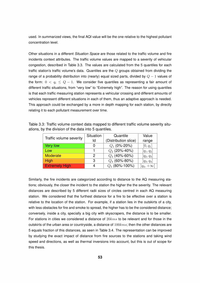
used. In summarized views, the final AQI value will be the one relative to the highest pollutant
concentration level.
Other situations in a different Situation Space are those related to the traffic volume and fire
incidents context attributes. The traffic volume values are mapped to a severity of vehicular
congestion, described in Table 3.3. The values are calculated from the 5 quantiles for each
traffic station’s traffic volume’s data. Quantiles are the Q groups obtained from dividing the
range of a probability distribution into (nearly) equal sized parts, divided by Q − 1 values of
the form: 0 < qi ≤ Q − 1. We consider five quantiles as representing a fair amount of
different traffic situations, from “very low” to “Extremely high”. The reason for using quantiles
is that each traffic measuring station represents a vehicular crossing and different amounts of
vehicles represent different situations in each of them, thus an adaptive approach is needed.
This approach could be exchanged by a more in depth mapping for each station, by directly
relating it to each pollutant measurement over time.
Table 3.3: Traffic volume context data mapped to different traffic volume severity situ-ations, by the division of the data into 5 quantiles.
Traffic volume severitySituation
IdQuantile
(Distribution slice)Valuerange
Very low 0 Q1 (0%-20%) [0, q1]
Low 1 Q2 (20%-40%) ]q1, q2]
Moderate 2 Q3 (40%-60%) ]q2, q3]
High 3 Q4 (60%-80%) ]q3, q4]
Extremely High 4 Q5 (80%-100%) ]q4,+∞[
Similarly, the fire incidents are categorized according to distance to the AQ measuring sta-
tions; obviously, the closer the incident to the station the higher the the severity. The relevant
distances are described by 5 different radii sizes of circles centred in each AQ measuring
station. We considered that the furthest distance for a fire to be effective over a station is
relative to the location of the station. For example, if a station lies in the outskirts of a city,
with less obstacles for fire and smoke to spread, the higher has to be the considered distance;
conversely, inside a city, specially a big city with skyscrapers, the distance is to be smaller.
For stations in cities we considered a distance of 20kms to be relevant and for those in the
outskirts of the urban area or countryside, a distance of 100kms; then the other distances are
5 equals fraction of this distances, as seen in Table 3.4. The representation can be improved
by studying the exact impact of distance from fire sources to the stations and taking wind
speed and directions, as well as thermal inversions into account, but this is out of scope for
this thesis.
53

Table 3.4: Fire incidents’ context data mapped to different fire severity situations, bythe creation of 5 circles of different radii around AQ monitoring stations.
Fire severity relative toAQ station location
Situation IdCity distancesrange (in kms)
Countryside range(in kms)
No fire 0 ]20,+∞[ ]100,+∞[
Very low 1 [16, 20] [80, 100]
Low 2 [12, 16[ [60, 80[
Moderate 3 [8, 12[ [40, 60[
High 4 [4, 8[ [20, 40[
Extremely High 5 [0, 4[ [0, 20[
The outcome of Context States and deducted situations are used in the monitoring views of
the MyAQI system, as well as in its prediction model. In the following section the selected
forecasting model and its interaction with context and situation variables is explained.
54

3.4 Prediction Model
The previous subsection introduced the necessary context attributes and situations for the
MyAQI system’s operation. Another critical building block of the system is the inclusion of a
prediction model, that consumes the environmental context information and forecasts values
for future time steps. The task to select a relevant prediction technique, that fits the data
at hand, arises. For this work we rely on the research explained in section 2 about existing
machine learning and AI data analysis methods. On of these trending and highly accurate
approaches is Deep Learning, specifically Deep Learning Neural Networks. Because the
nature of the AQ related data follows a time-series format, these networks have been already
applied to the AQ monitoring and forecast use case, presenting extremely promising results
and outperforming almost all of other older data based regression models. For these reasons
the MyAQI system uses a LSTM DNN for its prediction feature. In this subsection we introduce
some of the concepts relevant for a LSTM’s functioning.
3.4.1 Long Short-Term Memory Neural Network
A LSTM DNN is a type of gated RNN first introduced in (Hochreiter and Schmidhuber, 1997),
that keeps information for long time dependencies, which were neglected by former ANN
models. It consists of an input layer, that takes the incoming features, followed by one or more
recurrently interconnected hidden layers, also know as memory blocks, and an output layer,
that produces the final result for the regression. The main improvement of LSTMs takes place
in the memory blocks. Each block is composed by various memory cells (which in turn can be
connected to itself) and by multiplicative gates. The gates are for input, output and forgetting
tasks. These tasks can be mapped to read, write and reset operations, respectively. The input
gate controls if the cell’s internal state is to be affected by incoming signals and the output gate
controls if the result of the cell’s processing will affect other cells. But the novel concept in a
LSTM neuron structure is the forget gate, which resets the cells state once the information
held by it is outdated thus preventing the saturation of the squashing function, that occurs with
the out-of-bounds growth of a cell’s state. The state itself is maintained by the activation of
a self-connected linear unit-constant error carousel (CEC), which is part of the cells memory
and can stop any stimulus coming from the outside, thus retaining the same state over certain
periods of time. This feature allows LSTMs to solve the vanishing gradient problem, that is
accentuated with the increase of layers with different activation functions making the gradient
of the loss function approach zero, affecting the networks ability to train. Figure 3.2 describes
a single cell memory block for an LSTM network.
55

Figure 3.2: A LSTM memory block with one memory cell.
The input of the block is represented by Xt where X = (X1, X2 . . . , XN ) and Xi ∈ RT ; N
is the number of dimensions in the input, T the time lag and Y = (Y1, Y2 . . . , YN ) the output
values. For the MyAQI system’s AQ prediction use case, X vectors take the values of the AQ,
meteorological and extended context attributes; the Y vector takes the values of the desired
to-be-predicted pollutant’s predicted concentrations. The functions denoted in Figure 3.2 by
the free floating letters are characterised by the following equations:
ft = σ(Wf · [ht−1, Xt] + bf ) (3.1)
it = σ(Wi · [ht−1, Xt] + bi) (3.2)
Ct = ft ∗ Ct−1 + it ∗ tanh(WC · [ht−1, Xt] + bC) (3.3)
56

ot = σ(Wo · [ht−1, Xt] + bo) (3.4)
ht = ot ∗ tanh(Ct) (3.5)
where ft denotes the forget gate, it the input gate and ot the output gate. σ(·) stands for the
sigmoid function and tanh(·) the tanh function, defined in function 3.6 and 3.7, respectively.
Ct and ht are the activation vector for each cell and memory block, respectively. W represents
the weight matrix and b the bias vector.
σ(x) =1
1 + e−x(3.6)
tanh(x) =ex − e−x
ex + e−x(3.7)
Considering the LSTM’s structure and theory, its application to the MyAQI was to be done.
Figure 3.3 presents the structure for the LSTM model adapted to the MyAQI system’s features.
The inputs are given by the time series for AQ, meteorological and extended context variables.
The latter group are first transformed through the Situation Reasoning model to the values
relevant to each situation. Then, all the variables are normalized to values between 0 and
1, to immediately after be fed into the LSTMs layer. The DNN depends on some hyper-
parameters (such as batch size, hidden layers numbers, neurons numbers per layer, training
epochs, etc.) that have to be twitched and tested to achieve an heuristically best outcome. In
section 5 some work done to obtain the best possible values for these hyper-parameters for
the MyAQI AQ prediction is presented. With these parameters the LSTM’s training epochs are
executed, the error loss calculated and a validation set used for assuring the model fitness.
The outcome of the LSTM layer is forwarded to a fully-connected ANN (FCNN) and the result
of its execution are the predicted values for the desired pollutant (specified at the input, i.e.
P1(t+1) . . . P1(t+24)) for different time lags, if required. Lastly, the pollutant predictions are
used to reason the AQ situation at the given time point.
Finally, with the prediction model, the MyAQI system’s prediction and monitoring functioning
flow presented in Figure 3.1 has been completed. But obtaining the outcoming values from the
prediction are not enough, they have to be presented in a comprehensive and context-aware
57

Figure 3.3: The MyAQI system LSTM’s structure and general prediction work-flow.
manner to the end-users. The outcome of the forecasts and the current data is presented
through the MyAQI web-application visualization tools. These tools along with other key build-
ing blocks of the system’s implementation and design are presented in the next section of this
thesis.
3.5 Summary
This chapter of the thesis described the most relevant aspects of the context model used in
the MyAQI system. It defines some important theory to enable the modelling, then proposed
the list of Context Attributes together with their format, value range, unit of measurement and
example, and finally presented the situations in the Situation Space and their triggering factors.
The following step in this research will handle the implementation of the system, together with
the explanation of the prediction algorithm chosen and the role of context-awareness in this
process.
58

4 MyAQI Architecture and Implementation
In this chapter the details of the MyAQI system’s, architecture and implementation are pre-
sented, considering the theory and models presented in the previous sections.
4.1 System Architecture
In the previous chapter the main aspects of the critical functionalities of the MyAQI system
where explained. Context and situation modelling, as well as the prediction method to apply
where introduced. Considering these characteristics, we now present an architecture that will
suit the requirements of this system.
First, it is necessary to remind that these system, even though an IoT based system, is not
concerned with the creation and layering out of physical sensors. Given that the focus of the
thesis is to improve prediction accuracy by applying context-aware concepts into the process,
we utilize existing data streams from already functioning sensor networks, which are going
to be presented in section 5.1.2. Bearing this in mind, the architecture of the system starts
with the recognition of incoming AQ and context data streams and databases. This happens
in the Data Layer, which is encapsulated by the Backend or Server Layer. The formatted
data streams are passed to the Logic Layer, which prepares the context model, applies the
prediction algorithms and acts as an Application Programming Interface (API) to the Frontend
Layer, which in turn is responsible for Situation Reasoning and for presenting the data to the
user, through the Visualization Layer. Next we go over each layer and explain thoroughly their
parts and functionalities. Figure 4.1 gives an overview of the architecture and the technologies
that are used to implement each part.
4.1.1 Backend Layer
The backend layer encapsulates the Data Layer and the Logic Layer. It resides in the server
side and is tasked with preparing the context information for the Frontend Layer to be able to
reason the situations and present customize data to the user.
Data Layer it is responsible for storing, processing and formatting incoming streams of data
coming from different sources, such as third party APIs, historical data sets or live sensor
59

Figure 4.1: MyAQI system architecture and technologies for each layer’s implementa-tion.
nodes’ data. The most relevant data is:
• User profiles store the information regarding the system’s user, such as user id, email,
password, age, preferred AQI scale, last geo-position, the user’s questionnaire answers
and pollutant sensitivity levels.
• Air Quality data can come from different sources. For AQ characteristics in the state of
Victoria in Australia, for example, we use a data stream offered by the Victoria govern-
ment and save the some relevant information into our database, such as the AQ sensor
sites, the time basis for measurements updates, the available pollutants per sensor site,
amongst others. The individual measurements’ data (live and historical) is retrieved ev-
ery time from the API itself. The data is presented in such a way that the Frontend
Layer is agnostic of the source of the data and whichever format it had. AQI scales’
information is also stored in this database, each which their own categories, limits and
health messages.
• External context data is also stored in this layer. Traffic APIs and historical datasets
provide the required information to extend the understanding of the user and aid the AQ
prediction process. Live bushfire feeds also expand the user’s understanding of the AQ
sources and historical databases help improve the accuracy of forecasting techniques.
60

This data, independent of source, is formatted in a way that the frontend can be unaware
of the data source, because the presentation is kept constant.
• Prediction data is saved to allow the prediction algorithm to work with data of previously
ran forecasting processes. After a prediction sequence is run, the data is then stored in
a format that the same algorithm can use as an input in oncoming loops.
The final goal of the data layer is to make the adding of APIs and datasets general, in a way
in which user’s can add their own. For example, if users own an AQ personal sensor they
could add plug and play it to the system and obtain information that the device provides in the
MyAQI frontend. Next, the data streams made available by the data layer is consumed by the
logic layer which will format it into the context model and apply the prediction algorithms on it.
Logic Layer contains the business logic for the MyAQI system. It receives the information
from the data layer and process it in such a way that the functionalities required by the user
are covered, and sends the resulting information to the Frontend Layer. It is divided into three
modules.
• Context modelling handles the transformation of the raw data received from the data
layer to a format that fits into the context model described in section 3. It maps each
API or database data into the required Context Attributes allowing the next module to
apply the prediction algorithms on top of it.
• Prediction algorithm selector is a meta model selector, which means that it can apply
different algorithms depending on the system’s configuration. The algorithms expect
the data to be formatted so that it can be directly applied in their logic. A more in-
depth explanation about the algorithm selection and data flow will be presented in the
implementation subsection 4.2.
• API administers the frontend calls from the user devices to get the required data. Re-
quests for information may trigger certain functions in the Backend Layer or they may
just interact directly with the Data Layer to retrieve simple static information. The API
module should be independent of framework technology and should adapt to the end-
user device’s requirements and the required functionality. For demonstration purposes,
a Hyper Text Transfer Protocol (HTTP) Representational State Transfer (RESTful) API,
for frontend triggered requests, and a Web Sockets (WS) API, for notification purposes,
are implemented.
The Backend Layer will prepare all data necessary for frontend clients to retrieve and use.
61

4.1.2 Frontend Layer
Having a backend system in place, as explained in the previous sub-section, we need a client
that can consume the prepared information and present it to the user in a customized and
context-aware form; such is the task of the Frontend Layer. It consists of only one module, the
Visualization Layer which in turn is made of three main parts, each of which will be run on
an end-user device.
• API consumer handles the interaction and calls to and fro the backend interfaces. It
also prepares the data for the situation reasoner and visualization interface, given that
some data formats vary depending on the source (i.e. Web Sockets vs. RESTful API).
• Situation reasoner contains all the logic for the Situations Space define in chapter
3. It will compare the data obtained from the APIs against the rules defined for each
situation and give the resulting output to the visualization interface, to be rendered to
the user.
• Visualization interface consists mainly of display technologies that lets the user inter-
act with the system. It shows the outcomes from the whole AQ monitoring and predic-
tion process to the end-user. It also lets users actuate over the system, in that it gives
the option to customize details of the user profile and visualization settings.
The whole system architecture is designed in a way that prioritizes the customizability and
context-awareness execution. But it is also simple to notice that the main concept behind
the architecture is that of a server/client Web System, following the Model-View-Controller
(MVC) framework. The model being the Data Layer which is mapped with a Object-relational
Mapping (ORM) to the Logic Layer, which is the controller and where the data is transformed
and worked upon, and finally, the view which in the frontend acts as the interface towards the
outside world.
4.2 Implementation
In the previous chapters the main functionalities, models and goals of the MyAQI system
where introduced. In this section the implementation of the system is presented. Considering
the system architecture presented in section 4.1, the following step is to map each structural
element to hardware equipment and it’s functioning software.
62

4.2.1 Hardware
Given that the system is divided in two mayor layers, they both need to run on devices that
match their requirements. The backend layer is a server node that requires high availability,
reliability and bandwidth, to be able to interact with many clients at the same time. And the
frontend devices should be any devices that user’s have regular access to, i.e. laptops, mobile
phones and tablets.
The server characteristics chosen for the purpose of the experiments in this system is a Linux
18.04 Server with 500GB of storage, 16B of RAM and a 4-cores 2.60GHz processor. The
server is hosted in the Deakin University’s Intranet and available through http://schurholz.it.deakin.edu.au/.
The storage size and other characteristics of the server are due to the fact the prediction al-
gorithms can be quite expensive in resources and the server must still be able to function as
a web server on the mean time.
The end-user devices can be any modern laptop, mobile phone or tablet, given that the
purpose of the system is to be available to any user. The only condition is that the devices
can render a modern version of any web-browser and display it to the user. For the purpose
of the experiments of this research a Lenovo X1 Carbon laptop, a Huawei P8 mobile phone
and a 2017 iPad tablet were used, as shown in Figure 4.2.
Figure 4.2: The MyAQI system rendered on different end-user devices, for more ac-cessibility.
63

The goal of the MyAQI system is to be able to be accessible to as many users as possible and
given the ubiquity and cross-platform characteristics of web browsers, the best approach is to
develop a web-system with a responsive frontend web site for the prototype.
4.2.2 Software
For each previously mentioned layer different software tools have been used to accomplish
their goals. Figure 4.1 shows the main frameworks used for each module, but there are more
libraries involved in the process. As a rule for all the technologies chosen, we expect the tech-
nologies to be open-source, free and with a sufficient amount of documentation, community
and research involvement to be able to qualify for this research. Next, the reasons for why
each tool was chosen are explained.
The Data Layer requires a database engine that is capable of handling large sets of data in
an organized way. The tool chosen is PostgreSQL, given the large acceptance in the devel-
opment community. It also carries the benefit of having the PostGIS plug-in, that allows the
database to run geographical queries, i.e. geo-locations that fall inside a given polygon area
of land. This is specially useful for querying the traffic and bushfire datasets for the extended
context. Besides the interaction with databases, the Data Layer also handles requests from
external third party APIs. The tool handling this communications is the Requests python li-
brary. Given that the Logic Layer is going to be programmed in the Python programming
language, the choice of the aforementioned frameworks makes more sense; the ORM to map
database records to memory objects is the Psycopg2 python library.
As previously explained the Logic Layer will be mostly programmed using Python. The context
modelling, bundling and interaction will be handled by the Django web framework. It is a well
established tool, with a vast on-line community and used amongst a large set of web systems.
The seamless interaction with the PostgreSQL database records is also of great benefit. For
the development of the prediction algorithms the python libraries Tensor Flow and Keras were
applied. They are largely accepted in the research community as tools to implement robust
algorithms for data analysis using ANNs and DL. [TO-DO, explain more about the prediction
tools]. At the very front of the Backend Layer and acting as a RESTful API, the python library
Django Rest Framework (DRF) is used. It is a third party tool developed to fit into the Django
framework and is used in a large number of projects. The requests to the API are handled by
an NGINX HTTP server, which is together with Apache HTTP, one of the most widely used
ones. The other interface, besides HTTP, is a Web Sockets system, which is developed using
64

the Django Channels python library and Redis as a memory data structure framework for
faster socket connection handling.
The Frontend Layer requires a framework that will easily produce an interactive visualization
application, that is responsive and compatible with different devices. For that purpose, we se-
lected the ReactJS framework, because it is widely used, is constantly maintained and has a
vast support community. It is a cross-platform technology as it uses mainly a modified version
of JavaScript (called JSX), Hyper Text Mark-up Language (HTML) and Cascade Style Sheet
(CSS), and can be rendered in any modern browser. React also offers a large number of plug-
ins designed to aid with different common tasks in web applications. The main plug-in used
in the MyAQI system is the Redux tool, that helps keep the state of the application updated
during its execution, triggers API requests, updates views and re-renders components of the
web site. Other important plug-in is the GoogleMapsAPI, which aids in visualizing geographi-
cal relevant data, such as AQ information, traffic and bushfire data. Other minor libraries and
tools are used to simplify the development of the application. For exact versions and links for
tools and plug-ins see APPENDIX 1.
As part of the Frontend layer we designed an end-user interface considering that the interface
of any context-aware system has to convey a sense of individualization to the user. It has to
allow them to customize many characteristics, like colours, tool-placing, element sizes, etc.
It also has to be simple to understand and easy to use. The design concept adopted for the
MyAQI is that of a Dashboard, which is widely used in monitoring oriented applications. All
the views are be easily accessible and the user is allowed to customize certain aspects of the
application’s behaviour, besides the context model. A map of the navigation of the web app
can be observed in Figure 4.3.
The navigation of a user session in the web application starts in the Authentication module.
One of the requirements from the MyAQI Context Model is that user have a related ID. For
these purpose, the system lets new users register in the Registration view. For already signed-
up users, the access to the web application is through the Login page, where only user-name
(User ID) and password are asked for. Once authenticated the user is redirected to the Dash-
board. From this view, users can navigate to any information panel they require. First, there
is the AQI Monitoring module, which contains the AQI Historical Map and the AQI Forecast
Map pages. On these sites users can interact with data coming from different sources that
reveal the AQI and pollutants’ levels from past, current and future time intervals and from
different locations. Another panel accessible to the user is the Pollution Sources module,
which contains two views. First, there is the Traffic Map view, where users can understand the
traffic related issues and traffic flows that could be causing air pollution problems. Similarly,
65

Figure 4.3: The MyAQI web application’s views and navigation.
the second view, the Fire Map, shows fire related issues on a map, from which users can
grasp the effect of bushfires or household fires that could be causing a rise in Air Pollutants
around a region. Finally, the logged-in user can customize the experience given by the MyAQI
in the Customization module, which contains the User Profile and Settings panels. The first
one, gives the ability to modify personal information, answer the pollutant sensitivity question-
naire, select the preferred AQI scale and preview the pollutant sensitivity levels, the AQI maps
overlays and colours and view the selected AQI scale information.
Another requisite for context-aware systems is the ability to configure the overall systems set-
tings on run-time. For this purpose an Administration Dashboard was developed. From this
dashboard, a user with higher level permissions can create, update or delete the information
that the web application will use. In 4.4 for example, administrators can modify the colours,
limit, descriptions, abbreviations, etc. of the AQI scales. Other scales can be seamlessly
added and the web application’s users will notice the change in real time.
The end-user interfaces allow users to interact with the system and also validate the context-
aware research goals of this thesis.
66

Figure 4.4: The MyAQI web application’s administration dashboard and AQI cate-gories example.
More information about the specific structure of the code both in the backend and frontend is
described in the appendix section APPENDIX 2.. Each of the layers is a separate system or
sub-system. So, a mean for communication must be considered.
4.2.3 Communication
As briefly mentioned in the previous sections the communication in the MyAQI system is
twofold. The first set of interactions happen between the system and the data sources re-
quired for each function. And secondly, the Frontend Layer requests information from the
67

Backend through HTTP and in both directions through WS, which is handled directly through
the Transmission Control Protocol (TCP). A diagram of some example communications can
be observed in Figure 4.5.
Figure 4.5: The MyAQI system’s flow of information and communication protocols.
Note that frontend devices can communicate with third party APIs to consume data directly,
if it is for visualization purposes only. But any data that has to be processed by the context
model for AQ monitoring or prediction purposes has to be queried via the MyAQI server. The
WS server tuns in a different server and is in charge of handling notifications with urgent
information to users, i.e. when a pollutant concentration peak was measured in the recent
past.
68

4.3 Summary
This chapter described the process of developing the whole MyAQI system. From the archi-
tecture that guided the technology selection, passing through the necessary equipment and
devices for its functioning, through the software choices to achieve the desired outcomes, the
networking requirements that make possible the communication between layers, the interface
design to allow the user interaction with the system, to the very development process gone
through to be able to create the application. The completion of the system is only a starting
point for the goal of this research, which is to experiment and obtain results that can answer
the research objectives. Considering this, the experiment setup and the results are presented
in the following chapter.
69

5 EXPERIMENTS AND RESULTS
This chapter lays out the details of the MyAQI system’s, experiments and their results, as well
as the sustainability analysis performed on the proposed model and implemented prototype.
5.1 Experiments
The previous section introduced the architecture and implementation of the MyAQI system
and highlighted its different building blocks. The goal of the system is to prove the advantages
of context prediction, as well as proving its usability in a real-case scenario. This section
presents the experiments that were undertaken to specifically tackle those objectives. First
experiments’ location, setup and structure is explained, and later the datasets used to “fuel”
the system and create the necessary context are described.
5.1.1 Experiment Setup
Considering that the use case example presented in section 1 occurs in Melbourne, Australia,
and the propensity of the region to suffer under large bushfires on the late summer and early
autumn months, the experiments will take place in the Victoria state in Australia, specifically
in the greater Melbourne area. The goal of the experiments is to prove that the inclusion of
Context Aware concepts in AQ prediction and monitoring can improve the prediction accuracy
and user-experience.
For the prediction accuracy measurements a selection of the data for the input layer of the
prediction model (described in section 3.4) has to be done. Given the large amount of data that
can be collected for each context attribute, a smaller subset of the whole available datasets
(explained in section 5.1.2) has been used. Only data between the first of January 2017
and the first of January 2019 is considered, due to the datasets availability. Then, only four
weather and pollutant measuring stations are considered. The criteria for their selection is the
impact of the extended context variables on them. Usually the urban locations that suffer most
from large wildfire are the outskirts of cities, while those who suffer most from traffic pollution
are located close to the city centre. Thus, two stations for the each case where selected, the
Alphington and Melbourne CDB stations are situated in Melbourne’s centre area with huge
vehicle crossings around them; the Mooroolbark station lies in the eastern city suburbs, close
70

to forest and grassland covered area, prone to summer fires; and lastly, the Traralgon station
is located in a separate town to the east of Melbourne called Traralgon as well, which sits near
vast areas of forests susceptible to large bushfires.
For each measuring station, one to four nearby vehicle crossing stations where selected to
obtain the number of vehicles driving past the site every hour. The only station that this
does not apply to is Traralgon, since there is no crossing being measured nearby the AQ
monitoring site and the traffic volume in the town is not relevant. For this station, and for
Mooroolbark, the fires that affect the nearby areas have to be considered for the context and
prediction models. A radius of 100 km is considered to encompass the fires that could affect
the pollutant concentration levels at the measuring sites. As shown in section 3.3, depending
on the distance from the fire, the effect on the measurements are larger or lower.
The complete experimental setup can be navigated and understood in through “Experiments”
view in the MyAQI web application, as seen in Figure 5.1. The data can be queried on specific
dates or played at different speeds to see its evolution throughout time and how each attribute
affects the others. Figure 5.2 shows a zoomed in view of the Melbourne CBD station sur-
rounded by the traffic volume measuring stations, the coloured streets (according to the traffic
situations); and on the right panel the actual values for the measured pollutants and AQI, as
well as the values for the traffic volumes and the existing fires in the influence area of the site.
The experiments as explained in the previous paragraphs, requires existing data sources that
feed each of the variables. The data shown on the panel and used in the experiments were
taken from different such sources and are defined in the following subsection.
5.1.2 Dataset Description
In section 3 the context and situations models were described. Each of those require data
sources to create a usable system and to test the proof-of-concept. Consecutively, the differ-
ent datasets used for the AQ, meteorological, traffic and fires attributes are presented.
5.1.3 AQ dataset
The AQ attributes required in the context model are the AQI and the PM2.5, PM10, O3 ,NO2,
SO2 and CO pollutants. As explained in the previous section (section 5.1.1), the experiments
71

Figure 5.1: MyAQI general experimental setup view on the “Experiments” view of theweb application.
and system are located in the Victoria region, thus a dataset found to be quite useful is the Air-
Watch live API maintained by Victoria’s AU-EPA branch. The data provided is both historical
and current (updated hourly), and has almost all context variables for many of the sensor sta-
tions distributed throughout Victoria, including meteorological data, such as Wavelet Decom-
position, Web Sockets and Temperature. For stations that do not measure all the pollutants,
only the relevant pollutants for the pollution sources in the area of the sensor will be used.
Figure 5.3 presents a panel in the MyAQI application, where users can retrieve historical and
current information on the measurements for each of the AQ stations and sensors available in
the dataset; and visualize the information as a chart or table.
For comparison purposes the MyAQI web-app also presents a view for AQ forecasts provided
by the WeatherBit API. It is a third party provider for external models such as the European
Centre for Medium-Range Weather Forecasts (ECMWF) weather and air quality datasets.
These models are run by Bureaus of Meteorology and other big organizations and use mod-
ern ensemble techniques for prediction and satellite atmospheric composition measurements.
These models rely solely on a time-series based analysis and forecast, they do not take ex-
72

Figure 5.2: MyAQI specific experimental setup view for the Melbourne CBD AQ stationon the “Experiments” view of the web application.
ternal context, such as pollution sources, as inputs.
5.1.4 Traffic volume datasets
One of the relevant pollution sources considered in the MyAQI model is the level of traffic
close to the desired prediction location. In Victoria, as in almost every major city in Australia,
the traffic lights system has the SCATS system (developed by the government of New South
Wales, Australia) integrated into their public roads network. This system has the function of
counting the amount of cars for every 15 minutes time span on each major crossing in the city
and adapting the traffic light operation according to it. The government of Victoria releases the
vehicle loads at the end of each month. This dataset was used for the prediction algorithm,
as input for traffic levels close to the prediction location. The information of traffic volume
for every 15 minutes where summed by the end of each hour, to correlate to the way the air
quality datasets are structured.
73

Figure 5.3: AQ sensor network used in the MyAQI system, provided by the localgovernment’s AU-EPA branch, in Victoria, Australia.
Other datasets used for monitoring in the MyAQI system are the VicRoads and the Bing Maps
live traffic incidents feeds, as well as the Google Maps traffic map layer. Even though the
information retrieved from the previous three sets were not used in the prediction algorithm as
inputs, they are used to aid the system’s end-users understanding of the current Air Quality in
their location. Figure 5.4 shows the traffic view on the MyAQI web application.
5.1.5 Fire incidents datasets
Another context attribute required for the context model explained in section 3 is information
about fire incidents (such as household fires or bushfires) close to the prediction location.
Again, the Victoria government offers such a dataset, as it keeps track of every fire in its
region since the 1930’s. For the purpose of this work only the information for season’s 2017
and 2018 where imported into the system. Every fire incident in the Victoria region present
in the dataset has a severity attribute, a geographical polygon describing its covering area,
74

Figure 5.4: Traffic incidents’ information used in the MyAQI system, provided by Vic-toria’s local government through the VicRoads platform; other sources are Bing Mapsand Google Maps.
a starting date and a referential identification field. The fire instances do not have an ending
date assigned, but it can be approximated depending on the severity of the fire, as shown in
Table 5.1; if a fire has a severity of BURNT_4, which is the worst case, the duration will be of
10 days and the ending date can be calculated from this value.
Table 5.1: Fire incidents, taken from the Victoria government’s fire incidents historicaldataset, depending on their severity.
Fire SeverityDuration(in days)
BURNT_1 3BURNT_2 5BURNT_3 10BURNT_4 15
Similar to the traffic information, there are other data streams available for fire incidents, that
can aid in the general understanding of current AQ levels by the users. The MyAQI system
75

consumes the data from the Victoria Emergency live feed. This information is updated every
minute and contains many types of urgent incidents in the region, including fire incidents.
Figure 5.5 shows the view on the MyAQI web-application that presents this information.
Figure 5.5: Fire incidents’ information view in the MyAQI system; data provided by theVictoria’s local emergency platform Victoria Emergency.
The resulting graphics and analysis are presented in the following section of this thesis.
5.2 Results
The previous subsection described the experimental setup and datasets laid out to obtain
measurements of the accuracy of the approach presented in this thesis. In this subsection
we present these results and explain their significance. First, data analysis work done on the
available input information, such as variable correlations and data histograms are described.
Then, the accuracy comparisons of the prediction algorithm are presented, comparing an
LSTM run considering external context attributes versus one without the extended information.
And, finally, the context-aware system views are presented, to complete the user-oriented
76

implementation of the MyAQI system.
5.2.1 Data Analysis
The information found in the datasets introduced in subsection 5.1.2 allow the application of
different analysis tools to understand the data that goes into the prediction algorithm and mon-
itoring systems, as well as explaining the relationship amongst different phenomena. Figure
5.6 describes the attributes for all the AQ stations for a short period of time. This allows to
understand the behaviour of the variables and see their relation at specific points in time. For
the two stations located in the outskirts of the Melbourne urban area, Mooroolbark and Traral-
gon, the fire activity is significant during the months of February through to May and impact in
some high peaks in PM2.5 and PM10 levels, rising the AQI as well. For the city-located stations,
Melbourne CBD and Alphington, the traffic levels influence in the fluctuation of pollutants suck
as PM2.5 and O3.
Another explicative analysis is obtained through correlation heat-maps. Figure 5.7 presents
for the four stations. We can conclude again, that in the city Fire has no incidence over AQI
levels, but traffic does, and the other way around on the countryside.
The previous figures show that there exists a correlation between the extended context vari-
ables and some of the pollutants. This helps to select the specific input variables for executing
the prediction of each pollutant.
5.2.2 Prediction Accuracy
Previously, the data analysis of the variables for each AQ measuring station was done. With
this information the prediction model was trained and tested. To proof the accuracy of the
model and the selection of variables, a comparison against the ground truth (the real values)
was made, as seen in Figures 5.8 and 5.9. The former presents the values for a one-hour-
ahead prediction of PM2.5 levels made on the Melbourne station, using only values for the
previous 24 hours on PM2.5 concentrations and the traffic volume information for four of the
traffic measuring stations, presenting a good performance. The latter figure shows the values
for a one-hour-ahead prediction of PM2.5 concentrations using NO2, SO2, PM10 and CO,
besides the traffic volume information for the closest traffic station to the AQ measuring station;
the outcome of this prediction is much more accurate given the higher availability of data.
77

(a)
0
500 AQI
0
200 PM2.5
0
100
200
PM10
2018/02/25 2018/03/22 2018/04/16 2018/05/11 2018/06/05 2018/06/300
2
4FIRES
(b)
0
200 AQI
0
50 PM2.5
0
20 NO2
0
100 PM10
0
1 CO
2017/03/12 2017/04/01 2017/04/21 2017/05/11 2017/05/310
5 FIRES
(c)
0
50
100
150
AQI
0
20
40
60
PM2.5
2018/04/26 2018/05/11 2018/05/26 2018/06/10 2018/06/250
1000
2000
TRAFFIC_4419
(d)
0
200 AQI
0
50 PM2.5
0
50 NO2
0
200 PM10
0
1 CO
2018/03/07 2018/03/27 2018/04/16 2018/05/060
2 FIRES
Figure 5.6: Measurements for the most relevant context variables all AQ measuringstations. (a) Mooroolbark measurements during the 2018 bushfire season, (b) Trar-algon AQ measuring station measurements during a 2017 bushfire period, (c) Mel-bourne CBD on a regular period of time and (d) Alphington context attributes mea-surements during a regular period of time.
78

AQI
PM2.5
O3 PM10
TEMP
WSPEED
WDIR
TRAFFIC_118
FIRE
S
AQI
PM2.5
O3
PM10
TEMP
WSPEED
WDIR
TRAFFIC_118
FIRES−1.00
−0.75
−0.50
−0.25
0.00
0.25
0.50
0.75
1.00
AQI
PM2.5
O3 NO2
SO2
PM10
CO TEMP
WSPEED
WDIR
FIRES
AQI
PM2.5
O3
NO2
SO2
PM10
CO
TEMP
WSPEED
WDIR
FIRES−1.00
−0.75
−0.50
−0.25
0.00
0.25
0.50
0.75
1.00
(a) (b)
AQI
PM2.5
TRAF
FIC_44
19
TRAF
FIC_44
05
TRAF
FIC_44
04
TRAF
FIC_44
06
FIRE
S
AQI
PM2.5
TRAFFIC_4419
TRAFFIC_4405
TRAFFIC_4404
TRAFFIC_4406
FIRES−1.00
−0.75
−0.50
−0.25
0.00
0.25
0.50
0.75
1.00
AQI
PM2.5
O3 NO2
SO2
PM10
CO TEMP
WSPEED
WDIR
TRAFFIC_4653
FIRE
S
AQI
PM2.5
O3
NO2
SO2
PM10
CO
TEMP
WSPEED
WDIR
TRAFFIC_4653
FIRES−1.00
−0.75
−0.50
−0.25
0.00
0.25
0.50
0.75
1.00
(c) (d)
Figure 5.7: Correlation map for all context variables for the countryside Mooroolbark(a) and Traralgon (b) AQ measuring stations; and city Melbourne CBD (c) and Alph-ington (d) AQ measuring stations.
The previous two results show the benefits of using traffic information for predicting PM2.5 val-
ues. And for the rest of the AQ stations, which are located in a more rural area, the prediction
is augmented by the use of fire incidents informations. Figures 5.10 and 5.11 present the
PM2.5 predictions on the Mooroolbark and Traralgon stations respectively. The first one uses
Furthermore, Table 5.2 shows the comparison of predictions’ MAE, RMSE, precision and cor-
relation (R) values for the four stations, once with extended context and once without against
the ground truth. For all stations except Alphington the improvement in prediction is clear
when using the extended environmental context. The case with Alphington can be interpreted
as a lack of correlation between extended context variables and the AQ in the area, probably
coming from another pollution source. Precision, which measures the accuracy of the classifi-
79

07/06 12
h07
/07 00
h07
/07 12
h07
/08 00
h07
/08 12
h07
/09 00
h07
/09 12
h07
/10 00
h07
/10 12
h07
/11 00
h07
/11 12
h07
/12 00
h07
/12 12
h07
/13 00
h07
/13 12
h07
/14 00
h07
/14 12
h07
/15 00
h07
/15 12
h
0
10
20
30
40
50 ground truthprediction
Figure 5.8: Melbourne CBD AQ measuring station PM2.5 levels prediction, consideringfour adjacent traffic stations.
cation of situations after the forecast, is always improved in the other three stations, specially
in Mooroolbark and Traralgon, which are influenced the most by bushfires.
5.2.3 Context-Aware Views
The previous subsection explains the performance benefits of the MyAQI extended context
prediction. In this section we introduce another contribution related to the user experience of
the web application itself. Given the context aware nature of the system, its reconfigurability
is essential to allow it to adapt to the user requirements. Thus, the application contains a view
of the user profile, where users can customise their needs and see the changes reflected
throughout the system. Figure 5.12 shows the configuration panel. End-users can change
their personal information, as well as answer health related issues, select their preferred AQI
scale and review their pollutant sensitivity levels.
Another important impact of context-awareness is the creation of personalized notifications
80

06/06 18
h06
/07 00
h06
/07 06
h06
/07 12
h06
/07 18
h06
/08 00
h06
/08 06
h06
/08 12
h06
/08 18
h06
/09 00
h06
/09 06
h06
/09 12
h06
/09 18
h06
/10 00
h06
/10 06
h06
/10 12
h06
/10 18
h06
/11 00
h06
/11 06
h06
/11 12
h06
/11 18
h06
/12 00
h
0
10
20
30
40
50
60 ground truthprediction
Figure 5.9: Alphington AQ measuring station PM2.5 levels prediction, considering NO2,SO2, PM10, CO and one traffic station levels.
about situations that could affect the users’ activity. Figure 5.13 presents the My Air Quality
Index (MyAQI) web application context-aware air quality monitoring notifications for users with
different sensitivity levels to main pollutants. It shows that Ana, who is has the most delicate
health condition, because of her asthma, receives more severe alerts for the same pollutant
levels. Bob is second and given his moderately unhealthy condition he receives more warning
for pollutant levels in some locations. Finally, Alice, who does not present any bad health
conditions, receives only alerts for those locations that have very high pollutant concentrations,
hence being unhealthy for everyone.
Finally, given the general lack of understanding of the AQI scale numbering and indexing
from the general public, it was critical to incorporate a visualisation tool that allows users to
understand the air quality measuring system in an easy way. Thus, a gauge allows the viewer
to know the current status while understanding the whole range of the indexes was created.
Figure 5.14 shows the visualisation tool in the web application with EEA AQI as preferred AQI
scale (the tool accepts all three AQI scales).
The results reflect a system’s capability for context-aware AQ monitoring and prediction. It
81

04/30 13
h04
/30 15
h04
/30 17
h04
/30 19
h04
/30 21
h04
/30 23
h05
/01 00
h05
/01 02
h05
/01 04
h05
/01 06
h05
/01 08
h05
/01 10
h05
/01 12
h05
/01 14
h05
/01 16
h05
/01 18
h05
/01 20
h05
/01 22
h05
/02 00
h05
/02 01
h
0
50
100
150
200
250
300 ground truthprediction
Figure 5.10: Mooroolbark AQ measuring station PM2.5 levels prediction, consideringPM2.5, PM10, one traffic station and fire incidents.
incorporates a robust prediction mechanism and allows the end-user to follow a customizable
experience of air pollution monitoring.
82

Figure 5.11: Traralgon AQ measuring station PM2.5 levels prediction, considering NO2,SO2, CO, temperature, wind direction, wind speed and fire incidents. The backgroundcolours correspond to the AU-EPA AQI categories, proving that the prediction of AQsituations is accurate.
83

Table 5.2: Comparison of MAE, RMSE, precision and R values for the predictionresults from the LSTM model with and without extended context values, for all four AQstations.
Performance Indicators
Station Attributes MAE RMSE Precision R
Traralgon AQ station +1hr PM2.5 predictionWithout Extended Context PM2.5, PM10, NO2,
SO2, CO1.678 2.411 0.916 0.776
With Extended Context + Fires 1.477 2.262 0.943 0.772Mooroolbark AQ station +1hr PM2.5 predictionWithout Extended Context PM2.5, PM10 4.295 6.769 0.872 0.583With Extended Context + Traffic, Fires 2.124 8.775 0.909 0.629Alphington AQ station +1hr PM2.5 predictionWithout Extended Context PM2.5, PM10, NO2,
SO2, CO1.364 1.922 0.956 0.788
With Extended Context + Traffic, Fires 1.389 1.949 0.957 0.791Melbourne CBD AQ station +1hr PM2.5 predictionWithout Extended Context PM2.5 2.869 4.115 0.912 0.233With Extended Context + Traffic 2.797 3.85 0.93 0.353
Figure 5.12: The MyAQI web application user profile editing view, for a more person-alized experience of air quality monitoring.
84
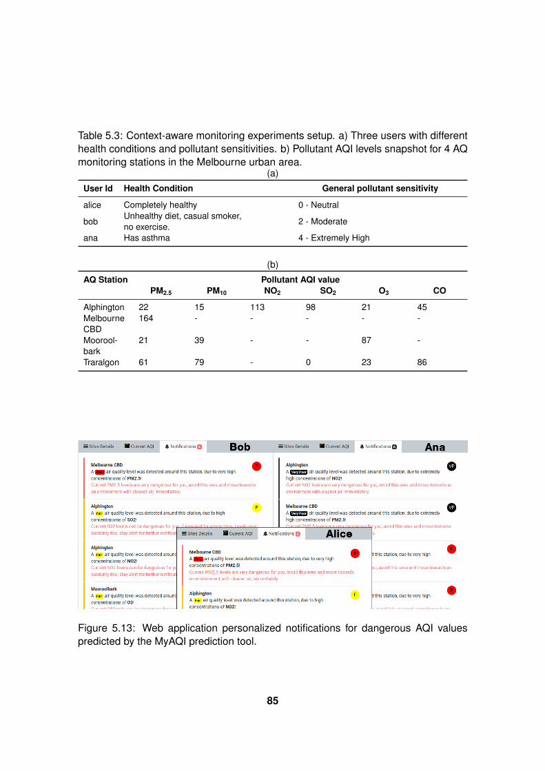
Table 5.3: Context-aware monitoring experiments setup. a) Three users with differenthealth conditions and pollutant sensitivities. b) Pollutant AQI levels snapshot for 4 AQmonitoring stations in the Melbourne urban area.
(a)
User Id Health Condition General pollutant sensitivity
alice Completely healthy 0 - Neutral
bobUnhealthy diet, casual smoker,no exercise.
2 - Moderate
ana Has asthma 4 - Extremely High
(b)
AQ Station Pollutant AQI valuePM2.5 PM10 NO2 SO2 O3 CO
Alphington 22 15 113 98 21 45MelbourneCBD
164 - - - - -
Moorool-bark
21 39 - - 87 -
Traralgon 61 79 - 0 23 86
Figure 5.13: Web application personalized notifications for dangerous AQI valuespredicted by the MyAQI prediction tool.
85

Figure 5.14: MyAQI web application view using the context-aware visualisation toolfor better AQI understanding.
86

5.3 Sustainability Analysis
The research work and results presented in the previous sections of this thesis have been
developed as part of the Erasmus Mundus Joint Master’s Degree for Pervasive Computing and
Communications for Sustainable Development (PERCCOM) program (Kor et al., 2019). This
program makes an emphasis on the sustainability aspects of Information and Communication
Technology (ICT) projects, hence it is very important to state the sustainability analysis of this
work. But first, it is important to define sustainability and its connection to the ICT environment.
A widely accepted definition of sustainable development was first mentioned in the Brundt-
land Report (Brundtland et al., 1987). The definition reads, that something can be considered
sustainable if “it meets the needs of the present without compromising the ability of future
generations to meet their own needs”. Today’s way of doing business is going the opposite di-
rection. We, as a society, are vastly prioritizing short-term economic growth for the enrichment
of a few people and are neglecting the dangerous consequences towards the environment that
these can bring. It is the same in the ICT area, where projects and companies prioritize their
economic performance over their impact on the environment. Therefore, a thorough screen-
ing must be done at the conception of every ICT project in order to minimize the impact of the
out-coming product on the health of the environment and people depending on such health.
To understand this impact of this project we utilize a tool described in (Duboc et al., 2019). It
consists of a five-pillar scheme, in which each pillar represents a field of our societal mesh on
which the project can have an impact. Each field can be affected by three different levels of
effects, a structural effect, an enabling effect and an immediate effect. The pillars and their
effects on this outdoor air prediction project are the following:
1. Economic: A structural effect on the economic area is that by making air pollution lev-
els public, the mitigation of their emissions will take more importance over economic
growth during important decisions, due to transparency and consciousness of the com-
munity (seen as a chain effect from the social pillar). The availability of forecasted AQ
levels can enable companies to make decisions to mitigate their impact and avoid fines,
having an enabling effect on from the project and laying the foundations for more trans-
parency. Finally, as an immediate effect, citizens will be able to avoid polluted areas in
cities leading to less health complications and their expenses on medicines and med-
ical attention will drop, having a positive economic impact for them. This last effect is
triggered by the individual immediate effect of users avoiding polluted areas.
2. Technical: Context-aware systems allow new data sources and prediction algorithms to
87

be seamlessly added to the platform, depending on everyone’s needs, enabling more
customizable content for citizens, co-enabling better decisions for businesses for sus-
tainable objectives and an overall awareness of the environment (as presented by the
structural effect in the environment pillar). As an immediate effect, we take the avail-
ability of a developed system that extends the context for AQ levels predictions.
3. Environmental: a clear structural effect on the environment is that individuals, organi-
zations and governments are more aware of the impact that each has on the AQ and
can, thus, make more informed eco-friendly decisions.
4. Individual: users can be prevented from going to hazardous areas, with high air pollu-
tion levels, by receiving constant and personalized updates on AQ. But not everything
has a positive effect for end-users, because they could develop a dependability on the
system that can reduce their ability to decide and listen to their own intuition. Constant
paranoia can arise from the dependence of users; so the application should be able to
show confidence levels on the predicted and monitored values, to leave space for peo-
ple’s common sense. Finally, as a more structural effect, individuals can demand better
policies and regulations from authorities, given that they have access to the same trans-
parent information, enabled by the social effect of communities knowing the sources of
pollution.
5. Social: communities will know the pollution levels and performance on their living ar-
eas, they can share the effects on how these levels affect each of them and demand
better managing of AQ from their communal authorities. This pillar is tied closely to the
previous one and enabled by transparency from governments and businesses.
The whole impact of this work on the afore mentioned pillars can be clearly seen in Figure
5.15.
5.4 Summary
In this chapter, the setup for the experiments that prove the theoretical work of previous sec-
tions is described, as well as the required datasets and information used in their execution.
Then, the obtained results and outcomes of the system are presented, which showed promis-
ing values and improvements for context-aware systems. Lastly, the performed sustainability
analysis proved that the proposed approach can provide benefits to important sectors of to-
day’s society if applied correctly. In the next section, conclusions are drafted for all the work
88

Figure 5.15: Sustainability analysis in the economic, technical, environmental, indi-vidual and social pillars of this work.
presented in this thesis, some limitations encountered in the planning and execution process
are mentioned and potential future work in this topic is discussed.
89

6 CONCLUSIONS AND FUTURE WORK
This chapter contains the conclusions for the overall work in this thesis, with emphasis on the
contribution, some limitations encountered during the process, and possible future work in the
topic’s area.
6.1 Conclusions
The main goal of the research done in this thesis was to research and propose a context-
and situation model for AQ monitoring and prediction systems that could prove the advan-
tages of context-aware computing when applied in air quality monitoring field. Context-aware
systems require a high level of personalisation and augmented information to allow users to
interact with it in a friendly and helpful manner. Also, the system was required to predict future
concentrations of pollutants with high accuracy and using extended context information in the
process.
The contribution of this work is the proposed context-aware model and system architecture for
AQ monitoring and prediction and we prove it by implementing the MyAQI system. It includes
the proposed context- and situation model, the selected prediction algorithm, a thorough ar-
chitectural design, the implementation, the coupling with selected data sources and the layout
of experiments to prove the expected performance of the system. A web application was de-
veloped to provide a user-friendly interface to allow user interaction with the monitoring and
prediction functionalities. The application is a customisable tool that gives users a highly indi-
vidualised experience and augments their understanding of the air pollution problem. All the
data used in the system was obtained from trusted historical and current data sources and
reflect real-life situations obtained from the Victoria EPA in Australia, allowing for an objective
assessment of the research results.
Another contribution of the MyAQI system is the use of extended environmental context
sources on the AQ prediction problem, by adding data directly linked to the pollution sources.
As the results section (5) of this thesis shows, by adding these sources the prediction accu-
racy was improved for 3 out of 4 AQ station. By applying pollution sources as input to the
prediction model, the unavailability of AQ attributes (e.g., airborne pollutants measurements)
can be covered and hence the prediction improved. Complying with the context-awareness
of the system, predictions also offer augmented and customised information to the end-users,
90
by relating forecasts to possible pollution sources and showing the AQI level according to the
users’ health conditions.
In this research we do not focus on optimising the prediction algorithm or on developing a novel
prediction algorithm due to the limited scope of this thesis. The background and literature
review information of Chapter 2 was intended to select the best model to be used in this
system. The usage of real-life data sources allows for a good assessment of the system’s
operation, but it also introduces some limitations, as there only exists information for certain
locations and some data might have disturbances, due to malfunctioning of the measuring
devices. This reflects on having to use existing measuring stations to simulate the locations
of users; ideally each user would carry an air pollution device constantly with them and the
network of these devices would yield a more dynamic range and wider covering result.
Finally, the MyAQI system, implemented in this work, provides a proof-of-concept of a context-
aware system for the use case of AQ monitoring and prediction in the real-world scenario of
the Melbourne area in Victoria, Australia. It showed the benefits that can be drawn from
using existing IoT data sources and extracting more information from them by relating them to
real-life situations and phenomena.
6.2 Future Work
Considering the contributions and foundations laid out in this research, further research can be
done. The pollution sources used in the MyAQI system traffic and fire incidents, for instance,
are only two members of a large group, which includes factories, commercial businesses,
household artefacts, air planes, gas pipeline leaks, etc. Extreme natural phenomena can also
be taken into account, such as thermal inversions, volcanic eruptions, as they exacerbate,
diminish or contribute directly to air pollution. As mentioned in the previous section the pre-
diction algorithm could be improved and optimised as well. Furthermore, different prediction
models could be selected for different situations and locations, depending on their suitabil-
ity. An ensemble model can provide the best outcomes of different approaches for a specific
scenario.
Lastly, the larger goal of a context-aware system is to be data source and use case indepen-
dent. The MyAQI system covers the specific AQ monitoring and prediction use case and acts
as a prototype for it, but it could be potentially extended to allow the coupling of other datasets
and context-situation logic to cover other real-life issues.
91

APPENDICES
92

APPENDIX 1. Development Tools
Section 4 explains the implementation process for the MyAQI system and mentions software
tools and frameworks used for this process. Here we provide a list of names and links to each
mentioned tool’s resources.
• Bing Maps API: http://dev.virtualearth.net/REST/v1/Traffic/Incidents/
• Core-UI: https://coreui.io/
• Django Channels: https://github.com/django/channels
• Django Rest Framework: https://www.django-rest-framework.org/
• Django: https://www.djangoproject.com/
• Google Maps JavaScript API: https://developers.google.com/maps/documentation/javascript/tutorial
• Keras: https://keras.io/
• Matplot Lib: https://matplotlib.org/
• Pandas: https://pandas.pydata.org/
• PostGIS: https://postgis.net/
• PostgreSQL: https://www.postgresql.org/
• ReactJS: https://reactjs.org/
• Sklearn: https://scikit-learn.org/stable/
• Tensor Flow: https://www.tensorflow.org/
• Victoria Emergency API: http://emergency.vic.gov.au/public/osom-geojson.json
• Victoria EPA AirWatch API: http://sciwebsvc.epa.vic.gov.au/aqapi/
• Victoria Roads API: https://traffic.vicroads.vic.gov.au/maps.js
• Weather Bit API: https://api.weatherbit.io/v2.0/forecast/airquality
93

APPENDIX 2. Source Code Most Important Features
Section 4 explains the development process for the MyAQI system and describes the project
structure for the two frontend and backend sub-systems. The two main layers (Backend and
Frontend) were implemented on different source codes, given that they are written in different
programming languages and are heavily decoupled programs. Each project has its own struc-
ture and lives in a separate GitHub repository. This appendix shows explains the sublayers
development process in more detail, presents the project structures and explains three of the
implemented core functions to enable the context- and situation model presented in Section 3.
Figure APPENDIX 2..1 and APPENDIX 2..2 show the structure for the Backend and Frontend
projects, respectively.
The MyAQI Frontend Project is structured as a React project. The actions module handles
the calls to the APIs and the structure of the received data. In the components module,
major blocks of HTML elements that share a common functionality are bundled together for
reuse. The container directory contains theme-related files, like the layout of components in
the web site’s dashboard. The reducers module contains the Redux functionality that keeps
every component up to date, after changes in the data flow happened or the user interacted
with components. Finally, the views folder contains the frames for the major views, shown in
Figure 4.3, where components are used to create the site’s layout. The source code can be
found in the https://www.github.com/dschurholz/myaqi-frontend.git repository. More in depth
information about the purpose of certain files can be found in APPENDIX 2..
The MyAQI Backend Project is structured similarly to a Django project. Each major function-
ality and its resources are bundled together in a “project app”. Each one has a set of ORM
models, which map database records to in-memory objects, RESTful views, which control the
API calls, a set of Uniform Resource Locator (URL) where the API calls will be handled and
serializers, which control the the formatting of incoming and outgoing data. Other files which
have more specialized functions are located in the Common app. The source code can be
found in the https://github.com/dschurholz/myaqi-backend.git repository. Some of the most
important features are described in APPENDIX 2., as well as the project’s file structure. One
critical part of the backend project is the forecasting app. It contains all the files necessary
for the creation of prediction-ready data files, that consist of the cured data for each context
attribute to be used as input for the forecasting algorithm; the files for training and testing the
LSTM model with that data; and files to create the data with the forecasting output to be con-
sumed by the system developed in the Frontend Project, which is exactly the next step in the
development face.
94
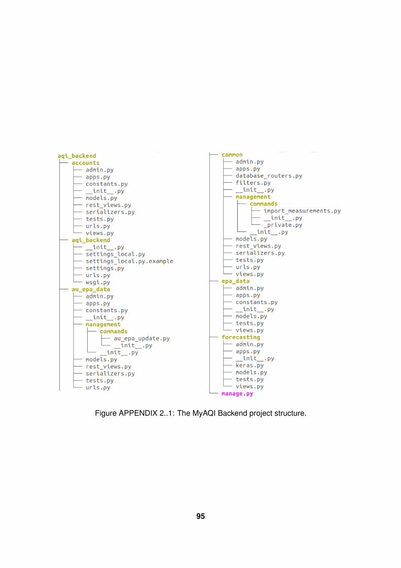
Figure APPENDIX 2..1: The MyAQI Backend project structure.
95

Figure APPENDIX 2..2: The MyAQI Frontend project structure.
96

The following function is used to determine the AQI category given a certain pollutant and a
list of its concentration levels for the AU-EPA AQI.
def get_categories(self, values, pollutant):
if self.abbreviation == ’AUEPA’:
aqi_cats = self.aqi_category_thresholds.filter(
pollutant=pollutant,
lower_threshold_value__isnull=False).order_by(
’lower_threshold_value’)
def get_cat(val):
for cat in aqi_cats:
if val < cat.upper_threshold_value:
return cat.abbreviation
return map(get_cat, values)
return None
The next function determines calculates the quantiles for the traffic flows for a traffic station,
in order to get the situation spaces.
@property
def quantiles(self):
data = TrafficFlow.objects.filter(
nb_scats_site=self.station_id).values_list(
’traffic_volume’, flat=True)
df = pd.DataFrame(data=data, columns=[’traffic_volume’])
return df.traffic_volume.quantile([0.2, 0.4, 0.6, 0.8])
The last function retrieves the fire incidents that happened in an area that are relevant to a
current location, which could represent an AQ monitoring station or the user’s position.
@classmethod
def get_fire_intersects_situation(
cls, areas, start_date=None, end_date=None, seasons=[]):
fires = cls.objects.all()
queries = [Q(geom__intersects=area) for area in areas]
query = queries.pop()
for item in queries:
query |= item
if start_date is not None:
fires = fires.filter(start_date__gte=start_date)
if end_date is not None:
97

fires = fires.filter(start_date__lte=end_date)
if len(seasons) > 0:
fires = fires.filter(season__in=seasons)
fires = fires.filter(query)
return fires
98

REFERENCES
Abowd, G.D., et al. (1999). Towards a Better Understanding of Context and Context-
Awareness. In: Gellersen, H.W., ed., Handheld and Ubiquitous Computing: First Inter-
national Symposium, HUC’99 Karlsruhe, Germany, September 27–29, 1999 Proceedings,
pp. 304–307. Berlin, Heidelberg: Springer Berlin Heidelberg. ISBN 978-3-540-48157-7.
Adhikari, R. and Agrawal, R. (2013). An Introductory Study on Time Series Modeling and
Forecasting. LAP LAMBERT Academic Publishing. ISBN 3659335088, 76 p.
Anagnostopoulos, C., Mpougiouris, P., and Hadjiefthymiades, S. (2005). Prediction intelli-
gence in context-aware applications. Proceedings of the 6th international conference on
Mobile data management, pp. 137–141. doi:10.1145/1071246.1071266.
Ashton, K. (2009). That ’internet of things’ thing in the real world, things matter more than
ideas. url: https://www.rfidjournal.com/articles/view?4986. Accessed:
2019-04-11.
Athira, V., Geetha, P., Vinayakumar, R., and Soman, K.P. (2018). DeepAirNet: Applying Recur-
rent Networks for Air Quality Prediction. Procedia Computer Science, 132, pp. 1394–1403.
ISSN 18770509, doi:10.1016/j.procs.2018.05.068, url: https://doi.org/10.1016/j.
procs.2018.05.068.
Bai, Y., et al. (2016). Air pollutants concentrations forecasting using back propagation neu-
ral network based on wavelet decomposition with meteorological conditions. Atmospheric
Pollution Research, 7(3), pp. 557–566. ISSN 13091042, doi:10.1016/j.apr.2016.01.004, url:
http://dx.doi.org/10.1016/j.apr.2016.01.004.
Barber, D. (2012). Bayesian Reasoning and Machine Learning. New York, NY, USA: Cam-
bridge University Press. ISBN 0521518148, 9780521518147.
Biancofiore, F., et al. (2017). Recursive neural network model for analysis and forecast of
PM10 and PM2.5. Atmospheric Pollution Research, 8(4), pp. 652–659. ISSN 13091042,
doi:10.1016/j.apr.2016.12.014.
Bikakis, A., Patkos, T., Antoniou, G., and Plexousakis, D. (2008). A Survey of Semantics-
Based Approaches for Context Reasoning in Ambient Intelligence. pp. 14–23.
Brockwell, P.J. and Davis, R.A. (2002). Introduction to Time Series and Forecasting , Second
Edition Springer Texts in Statistics. Springer. ISBN 0387953515, 434 p.
Brundtland, G., et al. (1987). Our Common Future (’Brundtland report’), Oxford Paperback
Reference. Oxford University Press, USA.
99

Canadian Government (2019). Humidex. url: https://www.canada.ca/en/
environment-climate-change/services/seasonal-weather-hazards/
warm-season-weather-hazards.html#toc7.
Catalano, M. and Galatioto, F. (2017). Enhanced transport-related air pollution prediction
through a novel metamodel approach. Transportation Research Part D: Transport and En-
vironment, 55, pp. 262–276. ISSN 13619209, doi:10.1016/j.trd.2017.07.009, url: http:
//dx.doi.org/10.1016/j.trd.2017.07.009.
Chen, L., et al. (2016). Spatially fine-grained urban air quality estimation using en-
semble semi-supervised learning and pruning. Proceedings of the 2016 ACM Inter-
national Joint Conference on Pervasive and Ubiquitous Computing - UbiComp ’16,
pp. 1076–1087. doi:10.1145/2971648.2971725, url: http://dl.acm.org/citation.
cfm?doid=2971648.2971725.
Cohen, A.J., et al. (2017). Estimates and 25-year trends of the global burden of
disease attributable to ambient air pollution: an analysis of data from the Global
Burden of Diseases Study 2015. The Lancet, 389(10082), pp. 1907–1918. ISSN
1474547X, doi:10.1016/S0140-6736(17)30505-6, url: http://dx.doi.org/10.1016/
S0140-6736(17)30505-6.
Domanska, D. and Wojtylak, M. (2012). Application of fuzzy time series models for forecasting
pollution concentrations. Expert Systems with Applications, 39(9), pp. 7673–7679. ISSN
09574174, doi:10.1016/j.eswa.2012.01.023.
Dong, M., et al. (2010). Expert Systems with Applications PM2.5 concentration prediction
using hidden semi-Markov model-based times series data mining. Expert Systems With
Applications, 36(5), pp. 9046–9055. ISSN 0957-4174, doi:10.1016/j.eswa.2008.12.017, url:
http://dx.doi.org/10.1016/j.eswa.2008.12.017.
Donnelly, A., Misstear, B., and Broderick, B. (2015). Real time air quality forecasting us-
ing integrated parametric and non-parametric regression techniques. Atmospheric En-
vironment, 103(2), pp. 53–65. ISSN 18732844, doi:10.1016/j.atmosenv.2014.12.011, url:
http://dx.doi.org/10.1016/j.atmosenv.2014.12.011.
Duboc, L., et al. (2019). Do we really know what we are building? Raising awareness of
potential Sustainability Effects of Software Systems in Requirements Engineering. In: 27th
IEEE International Requirements Engineering Conference. United States: IEEE Computer
Society.
100

Dutta, P., et al. (2009). Common Sense: Participatory urban sensing using a network of
handheld air quality monitors. Proceedings of the 7th ACM Conference on Embedded Net-
worked Sensor Systems, pp. 349–350. ISSN 160558519X, doi:10.1145/1644038.1644095,
url: http://dl.acm.org/citation.cfm?id=1644095.
EEA (2017). Air quality in Europe - 2017 report. Technical report. 13. European Environmental
Agency (EEA). ISBN 9789292139216.
EEA (2019). Air Index EEA. url: http://airindex.eea.europa.eu/. Accessed: 2019-
04-23.
EPA Victoria (2013). Future air quality in Victoria - Final report Future air quality in Victo-
ria - Final report. Technical report. Melbourne: Environmental Protection Agency Victoria
Australia.
Feng, X., et al. (2015). Artificial neural networks forecasting of PM2.5pollution using air mass
trajectory based geographic model and wavelet transformation. Atmospheric Environment,
107, pp. 118–128. ISSN 18732844, doi:10.1016/j.atmosenv.2015.02.030.
Fraser, A., et al. (2016). Services to develop an EU Air Quality Index. EEA Air Quality Index
Final Report.
Guillemin, P. and Friess, P. (2009). Internet of things strategic research
roadmap. url: http://www.internet-of-things-research.eu/pdf/
IoT_Cluster_Strategic_Research_Agenda_2009.pdf.
Henricksen, K. (2003). A Framework For Context-aware Pervasive Computing Applications.
Doctoral dissertation. The University of Queensland. 219 p.
Hochreiter, S. and Schmidhuber, J. (1997). Long Short-Term Memory. Neural Comput., 9(8),
pp. 1735–1780. ISSN 0899-7667, doi:10.1162/neco.1997.9.8.1735, url: http://dx.doi.
org/10.1162/neco.1997.9.8.1735.
Huang, C.J. and Kuo, P.H. (2018). A deep cnn-lstm model for particulate matter (Pm2.5)
forecasting in smart cities. Sensors (Switzerland), 18(7). ISSN 14248220, doi:10.3390/
s18072220.
Huang, S.F. and Cheng, C.H. (2008). Forecasting the air quality using OWA based time series
model. 2008 International Conference on Machine Learning and Cybernetics, 6(July), pp.
12–15. doi:10.1109/ICMLC.2008.4620967.
101

Kalisa, E., et al. (2018). Temperature and air pollution relationship during heatwaves in. Sus-
tainable Cities and Society, 43(June), pp. 111–120. ISSN 2210-6707, doi:10.1016/j.scs.
2018.08.033, url: https://doi.org/10.1016/j.scs.2018.08.033.
Kor, A.L., et al. (2019). Education in green ICT and control of smart systems : A first hand
experience from the International PERCCOM masters programme. In: 12th IFAC Sym-
posium on Advances in Control Education, ACE 2019. Philadelphia, United States. url:
https://hal.archives-ouvertes.fr/hal-02176670.
Kurt, A. and Oktay, A.B. (2010). Forecasting air pollutant indicator levels with geographic mod-
els 3 days in advance using neural networks. Expert Systems with Applications, 37(12), pp.
7986–7992. ISSN 09574174, doi:10.1016/j.eswa.2010.05.093.
Li, X., et al. (2017). Long short-term memory neural network for air pollutant concentration
predictions: Method development and evaluation. Environmental Pollution, 231, pp. 997–
1004. ISSN 18736424, doi:10.1016/j.envpol.2017.08.114, url: https://doi.org/10.
1016/j.envpol.2017.08.114.
Liu, W., et al. (2017). Neurocomputing A survey of deep neural network architectures and
their applications ☆. Neurocomputing, 234(December 2016), pp. 11–26. ISSN 0925-2312,
doi:10.1016/j.neucom.2016.12.038, url: http://dx.doi.org/10.1016/j.neucom.
2016.12.038.
Mayrhofer, R. (2004). An architecture for context aware management. Doctoral dissertation.
JOHANNES KEPLER UNIVERSITÄT LINZ.
Montgomery, D., Jenkins, C., and Kuhlaci, M. (2008). An Introduction to Time Series Foer-
casting. Wiley Series in Probability and Statistics. ISBN 3175723993.
Nurgazy, M., et al. (2019). CAVisAP: Context-Aware Visualization of Outdoor Air Pollution with
IoT Platforms. International Conference on High Performance Computing and Simulation
(HPCS).
Nurmi, P. and Floréen, P. (2004). Reasoning in context-aware systems. Helsinki Institute
for Information Technology, . . . , (1), pp. 1–6. url: http://www.cs.helsinki.fi/u/
ptnurmi/papers/positionpaper.pdf.
Oludare, I., Aman, J., and Abiodun, E. (2018). State-of-the-art in arti fi cial neural network
applications : A survey. Heliyon, (June), p. e00938. ISSN 2405-8440, doi:10.1016/j.heliyon.
2018.e00938, url: https://doi.org/10.1016/j.heliyon.2018.e00938.
102

Ong, B.T., Sugiura, K., and Zettsu, K. (2016). Dynamically pre-trained deep recurrent neural
networks using environmental monitoring data for predicting PM2.5. Neural Computing and
Applications, 27(6), pp. 1553–1566. ISSN 09410643, doi:10.1007/s00521-015-1955-3.
Padovitz, A., Wai Loke, S., and Zaslavsky, A. (2010). Towards a theory of context. Second
IEEE Annual Conference on Pervasive Computing and Communications, (Workshops, Per-
Com), pp. 38–42.
Peffers, K., Tuunanen, T., Rothenberger, M., and Chatterjee, S. (2007). A Design Science
Research Methodology for Information Systems Research. J. Manage. Inf. Syst., 24(3), pp.
45–77. ISSN 0742-1222, doi:10.2753/MIS0742-1222240302, url: http://dx.doi.org/
10.2753/MIS0742-1222240302.
Perera, C., Zaslavsky, A., Christen, P., and Georgakopoulos, D. (2014). Context Aware Com-
puting for The Internet of Things: A Survey. IEEE Communications Surveys Tutorials, 16(1),
pp. 414–454. ISSN 1553-877X, doi:10.1109/SURV.2013.042313.00197.
Perez, P. and Gramsch, E. (2016). Forecasting hourly PM2.5 in Santiago de Chile with em-
phasis on night episodes. Atmospheric Environment, 124, pp. 22–27. ISSN 1352-2310, doi:
10.1016/j.atmosenv.2015.11.016, url: http://dx.doi.org/10.1016/j.atmosenv.
2015.11.016.
Qi, Y., Li, Q., Karimian, H., and Liu, D. (2019). A hybrid model for spatiotemporal forecasting of
PM2.5 based on graph convolutional neural network and long short-term memory. Science
of The Total Environment, 664, pp. 1–10. ISSN 00489697, doi:10.1016/j.scitotenv.2019.01.
333.
Qiu, H., et al. (2013). Season and humidity dependence of the effects of air pollution on
COPD hospitalizations in Hong Kong. Atmospheric Environment, 76, pp. 74–80. ISSN
1352-2310, doi:10.1016/j.atmosenv.2012.07.026, url: http://dx.doi.org/10.1016/
j.atmosenv.2012.07.026.
Rabiner, L. (1989). A tutorial on hidden Markov models and selected applications in speech
recognition. Proceedings of the IEEE, 77(2), pp. 257 – 286.
Román, M., Hess, C., Cerqueira, R., and Campbell, R.H. (2002). A Middleware Infrastructure
For Active Spaces. IEEE Pervasive Computing, 1(4), pp. 74 – 83.
Russel, S. and Norvig, P. (2009). Artificial Intelligence a Modern Approach, third edit edn.
Prentice Hall. ISBN 9780136042594.
103

Shaban, K.B., Kadri, A., and Rezk, E. (2016). Urban Air Pollution Monitoring System With
Forecasting Models. IEEE Sensors Journal, 16(8), pp. 2598–2606. ISSN 1530-437X, doi:
10.1109/JSEN.2016.2514378.
Sheik Safeer, M.S. (2008). A Prediction System Based on Fuzzy Logic. The
World Congress on Engineering and Computer Science (WCECS), pp. 22 – 24.
ISSN 09507051, doi:10.1016/j.knosys.2014.09.010, url: http://www.iaeng.org/
publication/WCECS2008/WCECS2008_pp804-809.pdf.
Sigg, S., et al. (2012). Investigation of Context Prediction Accuracy for Different Context Ab-
straction Levels. IEEE Transactions on Mobile Computing, 11(6), pp. 1047–1059. ISSN
1536-1233, doi:10.1109/TMC.2011.170.
Sigg, S. (2008). Development of a novel context prediction algorithm and analysis of context
prediction schemes. Doctoral dissertation. University of Kassel. ISBN 9783899583922, 278
p.
Singh, K.P., Gupta, S., Kumar, A., and Shukla, S.P. (2012). Linear and nonlinear model-
ing approaches for urban air quality prediction. Science of the Total Environment, 426,
pp. 244–255. ISSN 00489697, doi:10.1016/j.scitotenv.2012.03.076, url: http://dx.doi.
org/10.1016/j.scitotenv.2012.03.076.
Sun, W. and Sun, J. (2017). Daily PM 2 . 5 concentration prediction based on principal compo-
nent analysis and LSSVM optimized by cuckoo search algorithm. Journal of Environmental
Management, 188, pp. 144–152. ISSN 0301-4797, doi:10.1016/j.jenvman.2016.12.011, url:
http://dx.doi.org/10.1016/j.jenvman.2016.12.011.
Sun, W., et al. (2013). Science of the Total Environment Prediction of 24-hour-average
PM2.5 concentrations using a hidden Markov model with different emission distributions
in Northern California. Science of the Total Environment, The, 443, pp. 93–103. ISSN
0048-9697, doi:10.1016/j.scitotenv.2012.10.070, url: http://dx.doi.org/10.1016/
j.scitotenv.2012.10.070.
United Nations (2018). The World ’ s Cities in 2018. Economics & Social Affairs.
USEPA (2013). Technical Assistance Document for the Reporting of Daily Air Quality - the Air
Quality Index ( AQI ). Environmental Protection, (May), pp. 1–28.
Wang, J. and Song, G. (2018). A Deep Spatial-Temporal Ensemble Model for Air Quality Pre-
diction. Neurocomputing, 314, pp. 198–206. ISSN 18728286, doi:10.1016/j.neucom.2018.
06.049, url: https://doi.org/10.1016/j.neucom.2018.06.049.
104

Weiser, M. (1999). The Computer for the 21st Century. SIGMOBILE Mob. Comput. Commun.
Rev., 3(3), pp. 3–11. ISSN 1559-1662, doi:10.1145/329124.329126, url: http://doi.
acm.org/10.1145/329124.329126.
Wen, C., et al. (2019). A novel spatiotemporal convolutional long short-term neural network
for air pollution prediction. Science of the Total Environment, 654, pp. 1091–1099. ISSN
18791026, doi:10.1016/j.scitotenv.2018.11.086, url: https://doi.org/10.1016/j.
scitotenv.2018.11.086.
Yin, P., et al. (2017). Particulate air pollution and mortality in 38 of China’s largest cities:
time series analysis. Bmj, 667(March), p. j667. ISSN 0959-8138, doi:10.1136/bmj.j667, url:
http://www.bmj.com/lookup/doi/10.1136/bmj.j667.
Zaslavsky, A., et al. (2016). D4.3 Theoretical Framework for Context and Situation Awareness
in IoT. bIoTope, (688203).
Zell, A. (1994). Simulation neuronaler Netze. R. Oldenbourg Verlag München Wien.
Zhao, H., et al. (2010). A GA-ANN model for air quality predicting. In: 2010 International
Computer Symposium (ICS2010), pp. 693–699.
Zhou, Y., et al. (2019). Explore a deep learning multi-output neural network for regional
multi-step-ahead air quality forecasts. Journal of Cleaner Production, 209, pp. 134–145.
ISSN 09596526, doi:10.1016/j.jclepro.2018.10.243, url: https://doi.org/10.1016/
j.jclepro.2018.10.243.
Zhu, S., et al. (2018). PM2.5forecasting using SVR with PSOGSA algorithm based on CEEMD,
GRNN and GCA considering meteorological factors. Atmospheric Environment, 183(July
2017), pp. 20–32. ISSN 18732844, doi:10.1016/j.atmosenv.2018.04.004, url: https://
doi.org/10.1016/j.atmosenv.2018.04.004.
105

106