Embed Size (px)
Citation preview

MASTER’s THESIS – RENEWABLE ENERGY MANAGEMENT
Cologne University of Applied Science - Institute for Technology and Resources
Management in the Tropics and Subtropics
and
Wuppertal Institut für Klima, Umwelt, Energie
DEVELOPMENT OF A PYTHON MODEL FOR ELECTRICITY RETAIL PRICES IN
GERMANY UNDER PRESENT REGULATORY FRAMEWORK AND FUTURE
EXPECTATIONS OF HIGH RE PENETRATIONS
Bilal Hussain
2017

1
Renewable Energy Management
Cologne University of Applied Science
ITT - Institute for Technology and Resources Management
in the Tropics and Subtropics
“DEVELOPMENT OF A PYTHON MODEL FOR ELECTRICITY RETAIL PRICES IN
GERMANY UNDER PRESENT REGULATORY FRAMEWORK AND FUTURE
EXPECTATIONS OF HIGH RE PENETRATIONS”
Thesis to Obtain the Degree of
MASTER OF SCIENCE
Renewable Energy Management
DEGREE AWARDED BY COLOGNE UNIVERSITY OF APPLIED SCIENCES
PRESENTS:
BILAL HUSSAIN
SUPERVISOR OF THESIS ITT
Prof. Dr. Johannes Hamhaber
SUPERVISOR IN WUPPERTAL INSTITUT FÜR KLIMA, UMWELT, ENERGIE:
Dipl.-Ing. Arjuna Nebel (Research Fellow)
DATE OF SUBMISSION
02.07.2017
presented by
Bilal Hussain Student no.: 01110987315 [email protected]

2
ACKNOWLEDGEMENTS
I would like to thank Mr. Arjuna Nebel for his effective supervision and kind guidance that
helped me in keeping my research efforts in right direction and in finishing all the milestones
well with in timelines. I am thankful to Prof. Dr. Johannes Hamhaber for his kind and
insightful feedbacks during execution of my thesis.
I would also like to appreciate DAAD for a generous two years scholarship to pursue the
amazing Masters course in Renewable Energy Management at ITT TH Koeln.
I am indeed grateful to my beloved wife Aenni for her tireless support and repeated
encouragements during the whole study period.

Table of Contents
3
TABLE OF CONTENTS ACKNOWLEDGEMENTS ..................................................................................................................................... 2
TABLE OF CONTENTS ......................................................................................................................................... 3
LIST OF TABLES ................................................................................................................................................. 5
LIST OF APPENDIX TABLES ................................................................................................................................ 6
LIST OF FIGURES ................................................................................................................................................ 7
ABSTRACT ......................................................................................................................................................... 9
1 INTRODUCTION ..................................................................................................................................... 10
1.1 ELECTRICITY RETAIL SECTOR OF GERMANY ......................................................................................................... 10
1.2 LATEST ELECTRICITY PRICE STATISTICS ............................................................................................................... 12
2 EEG-SURCHARGE ................................................................................................................................... 15
2.1 PERSPECTIVE ................................................................................................................................................ 15
2.1.1 Electricity Feed-In Act ..................................................................................................................... 15
2.1.2 EEG-2000 ........................................................................................................................................ 15
2.1.3 EEG-2004 ........................................................................................................................................ 16
2.1.4 EEG-2009 ........................................................................................................................................ 17
2.1.5 EEG-2012 ........................................................................................................................................ 18
2.1.6 EEG-2014 ........................................................................................................................................ 19
2.1.7 EEG-2017 ........................................................................................................................................ 20
2.1.8 EEG surcharge exemptions ............................................................................................................. 21
2.1.9 Historical development of EEG surcharge ....................................................................................... 21
2.2 MODEL DESCRIPTION ..................................................................................................................................... 23
2.2.1 Development of plant tariffs ........................................................................................................... 25
2.2.2 Estimating revenues of RE plant owners CEEG ................................................................................. 29
2.2.3 Scenario for EEG plants development ............................................................................................. 32
2.2.4 Scenario of EEG generation ............................................................................................................ 34
2.3 MODEL RESULTS AND VALIDATION ................................................................................................................... 35
3 NETWORK CHARGES .............................................................................................................................. 37
3.1 PERSPECTIVE ................................................................................................................................................ 37
3.1.1 Capital costs .................................................................................................................................... 39
3.1.2 Working capital for EEG sales ......................................................................................................... 40
3.1.3 System services costs ...................................................................................................................... 40
3.1.4 Avoided network charges ............................................................................................................... 41
3.1.5 Costs for retrofitting necessary to system frequency stability ........................................................ 42
3.1.6 Reduced grid charges...................................................................................................................... 42
3.1.7 Historical development of network costs........................................................................................ 42
3.1.8 StromNEV-19 surcharge ................................................................................................................. 44

Table of Contents
4
3.1.9 Offshore liability surcharge ............................................................................................................. 44
3.1.10 Interruptible load surcharge ........................................................................................................... 44
3.2 MODEL DESCRIPTION ..................................................................................................................................... 45
3.2.1 Transmission Costs (Tcosts) ............................................................................................................... 47
3.2.2 Distribution Costs (Dcosts) ................................................................................................................. 49
3.2.3 Services Costs .................................................................................................................................. 50
3.2.4 Scenario for grid investments ......................................................................................................... 53
3.3 MODEL RESULTS AND VALIDATION ................................................................................................................... 53
4 KWKG SURCHARGE ................................................................................................................................ 56
4.1 PERSPECTIVE ................................................................................................................................................ 56
4.2 MODEL DESCRIPTION ..................................................................................................................................... 57
4.3 MODEL RESULTS AND VALIDATION ................................................................................................................... 61
5 PRICE DEVELOPMENT TILL 2035 ............................................................................................................. 63
5.1 HOUSEHOLD CONSUMPTION ........................................................................................................................... 63
5.2 UNPRIVILEGED INDUSTRIAL CONSUMPTION ........................................................................................................ 63
5.3 PRIVILEGED INDUSTRIAL CONSUMPTION ............................................................................................................ 64
6 CONCLUSION & OUTLOOK ..................................................................................................................... 66
6.1 INTEGRATION OF RE GENERATION .................................................................................................................... 66
6.2 RISING RETAIL ELECTRICITY PRICES ..................................................................................................................... 68
6.3 RESEARCH GAPS AND FUTURE RESEARCH DIRECTION ............................................................................................. 69
REFERENCES .................................................................................................................................................... 71
Appendix A. Data relating to EEG Model ................................................................................. 74
Appendix B. Data relating to Network Charges Model ........................................................... 78
Appendix C. Data relating to KWKG model ............................................................................. 80

List of Tables
5
LIST OF TABLES
TABLE 1.1 ELECTRICITY RETAIL PRICE COMPONENTS AND MAJOR CONTROL FACTORS ........................................... 11
TABLE 1.2 AVERAGE RETAIL PRICE COMPONENTS ACROSS THREE CONSUMER CLASSES ON 1ST APRIL-2016 [SOURCE:
(BNETZA, 2016A)] ........................................................................................................................................ 14
TABLE 2.1 AVERAGE MARKETING FACTOR AND CLEAVAGE POINT PER TECHNOLOGY TO DISTRIBUTE HIGHER AND
LOWER MARKETING FACTORS AMONG HIGHER AND LOWER CAPACITY PLANTS [SOURCE: SELF, (BNETZA,
2016B)].......................................................................................................................................................... 31
TABLE 3.1 COST CATEGORIES CONSIDERED FOR REGULATED YEARLY REVENUES OF GRID OPERATORS .................. 39
TABLE 3.2 MODEL PARAMETERS: REFERENCE DATA POINTS FOR RDENNODELAY AND RDENDELAY CURVES ........... 51
TABLE 4.1 MODEL PARAMETERS: AVERAGE SUPPORT PERIODS (YEARS) FOR KWK PLANT CATEGORIES ............... 59
TABLE 4.2 MODEL PARAMETERS: P(CENTS/KWH) AND CF FOR KWK PLANTS ....................................................... 61

List of Appendix Tables
6
LIST OF APPENDIX TABLES
APPENDIX TABLE A.1 MODEL SCENARIO: YEARLY EEG CAPACITY (GWS) PER TECHNOLOGY .............................. 74
APPENDIX TABLE A.2 MODEL SCENARIO: YEARLY AVERAGE DEFAULT TARIFF (CENTS/KWH) PER TECHNOLOGY . 75
APPENDIX TABLE A.3 MODEL SCENARIO: YEARLY EEG GENERATION (TWH) PER TECHNOLOGY ......................... 76
APPENDIX TABLE A.4 MODEL RESULTS: YEARLY EEG SURCHARGE (CENTS/KWH) FOR PRIVILEGED AND
UNPRIVILEGED CONSUMER CATEGORIES ........................................................................................................ 77
APPENDIX TABLE B.1 MODEL RESULTS: YEARLY TRANSMISSION, DISTRIBUTION, SERVICES COSTS AND
AGGREGATED NETWORK COSTS ..................................................................................................................... 78
APPENDIX TABLE B.2 MODEL RESULTS: YEARLY AVERAGE NETWORK CHARGES FOR HOUSEHOLD/SME,
UNPRIVILEGED INDUSTRY AND STROMNEV-19 SURCHARGE FOR CATEGORIES A, B, C IN CENTS/KWH ........ 79
APPENDIX TABLE C.1 DATASET FROM (ÖKO-INSTITUT, 2015) FEATURING YEARLY ADDITIONAL CAPACITIES IN
MWS COMING UNDER KWKG SUPPORT MECHANISM CATEGORIZED AS PER CATEGORY M, C1, C2, C3 ........ 80
APPENDIX TABLE C.2 MODEL RESULTS: AGGREGATED YEARLY INSTALLED CAPACITIES, GENERATION, COSTS AND
KWKG SURCHARGE VALUES AS RESULTED FROM MODEL CALCULATIONS .................................................... 80

List of Figures
7
LIST OF FIGURES
FIGURE 1.1 VARIABLE PRICE COMPONENTS FOR DEFAULT SUPPLY CONTRACTS ACROSS FOUR HOUSEHOLD
CONSUMER CLASSES ON 1ST APRIL-2016 [SOURCE: (BNETZA, 2016A)] ......................................................... 13
FIGURE 1.2 SIGNIFICANT ELECTRICITY PRICE COMPONENTS ACROSS THREE CONSUMER CLASSES ON 1ST APRIL-2016
[SOURCE: (BNETZA, 2016A)] ........................................................................................................................ 14
FIGURE 2.1 YEARLY INSTALLED CAPACITIES UNDER EEG SUPPORT [SOURCE: (BNETZA, 2016B)]......................... 21
FIGURE 2.2 YEARLY ELECTRICITY GENERATION UNDER EEG SUPPORT [SOURCE: (BNETZA, 2016B)] ................... 22
FIGURE 2.3 YEARLY TOTAL EEG COSTS PER TECHNOLOGY [SOURCE: (BNETZA, 2016B)] ..................................... 22
FIGURE 2.4 SOLAR PLANT TARIFFS (RIGHT) AND INSTALLED CAPACITIES (LEFT) ORDERED IN ASCENDING ORDER OF
INSTALLATION YEARS AND DESCENDING TARIFFS (ZOOMED VERTICAL AXIS) ................................................ 26
FIGURE 2.5 BIOMASS PLANT TARIFFS (RIGHT) AND INSTALLED CAPACITIES (LEFT) ORDERED IN ASCENDING ORDER
OF INSTALLATION YEARS AND DESCENDING TARIFFS (ZOOMED VERTICAL AXIS) ........................................... 26
FIGURE 2.6 GAS PLANT TARIFFS (RIGHT) AND INSTALLED CAPACITIES (LEFT) ORDERED IN ASCENDING ORDER OF
INSTALLATION YEARS AND DESCENDING TARIFFS .......................................................................................... 27
FIGURE 2.7 WATER PLANT TARIFFS (RIGHT) AND INSTALLED CAPACITIES (LEFT) ORDERED IN ASCENDING ORDER OF
INSTALLATION YEARS AND DESCENDING TARIFFS (ZOOMED VERTICAL AXIS) ................................................ 27
FIGURE 2.8 GEOTHERMAL PLANT TARIFFS (RIGHT) AND INSTALLED CAPACITIES (LEFT) ORDERED IN ASCENDING
ORDER OF INSTALLATION YEARS AND DESCENDING TARIFFS (ZOOMED VERTICAL AXIS) ................................ 28
FIGURE 2.9 WIND-OFFSHORE PLANT TARIFFS (RIGHT) AND INSTALLED CAPACITIES (LEFT) ORDERED IN ASCENDING
ORDER OF INSTALLATION YEARS AND DESCENDING TARIFFS ......................................................................... 28
FIGURE 2.10 WIND-ONSHORE PLANT TARIFFS (RIGHT) AND INSTALLED CAPACITIES (LEFT) ORDERED IN ASCENDING
ORDER OF INSTALLATION YEARS AND DESCENDING TARIFFS ......................................................................... 29
FIGURE 2.11 PERCENTAGE VARIATION OF MODEL CALCULATIONS FOR EEG REVENUES OF PLANT OWNERS WITH
RESPECT TO REFERENCE REVENUES OF 2015 FROM (BNETZA, 2016B): WITHOUT CORRECTIONS (TOP), WITH
NON-MARKET RELATED CORRECTIONS (MIDDLE), WITH ALL CORRECTIONS (BOTTOM) ................................ 32
FIGURE 2.12 MODEL SCENARIO: START YEAR EEG CAPACITIES FROM 2015 TO 2035 ............................................ 33
FIGURE 2.13 MODEL SCENARIO: FUTURE DEVELOPMENT OF AVERAGE DEFAULT TARIFFS FOR EACH EEG
TECHNOLOGY [SOURCE: (OEKO-INSTITUT, 2016)] ......................................................................................... 34
FIGURE 2.14 MODEL SCENARIO: YEARLY GENERATION FROM EEG ELIGIBLE PLANTS FROM 2015 TO 2035 ........... 34
FIGURE 2.15 MODEL RESULTS: YEARLY CEEG FOR YEARS 2015-2035 AND REFERENCE PREDICTIONS FOR 2015-2017
FROM (BMWI, 2016B) ................................................................................................................................... 35
FIGURE 2.16 MODEL RESULTS: YEARLY BASE EEG SURCHARGE FOR UNPRIVILEGED CONSUMERS FOR YEARS 2015-
2035 VS RESULTS OF SAME PREDICTION FROM (OEKO-INSTITUT, 2016)......................................................... 36
FIGURE 3.1 YEARLY TRANSMISSION AND DISTRIBUTION COSTS 2009-2016 [SOURCE: (BEHRINGER, 2016)] ........... 43

List of Figures
8
FIGURE 3.2 IMPORTANT COST DRIVERS 2011-2015[ SOURCE: BNETZA, (HIRTH & ZIEGENHAGEN, 2013)] ............. 43
FIGURE 3.3 REGIONAL NETWORK CHARGES FOR HOUSEHOLD (LEFT), MEDIUM BUSINESS (MIDDLE) AND INDUSTRIAL
(RIGHT) CONSUMERS AS OF 01.01.2017 [SOURCE: BNETZA] ......................................................................... 43
FIGURE 3.4 SURCHARGE LEVELS FOR CATEGORY A, B, C FOR YEARS 2013-17 [SOURCE: NETZTRANSPARENZ.DE] 45
FIGURE 3.5 MODEL PARAMETER: RDENNODELAY AND RDENDELAY CURVES ............................................................ 52
FIGURE 3.6 MODEL SCENARIO: YEARLY RDENCUM AS PER TWO CURVES RDENDELAY AND RDENNODELAY ............... 52
FIGURE 3.7 MODEL SCENARIO: RE TARGET SHARE IN GROSS CONSUMPTION BY 2035 AND REQUIRED CUMULATIVE
INVESTMENTS IN TRANSMISSION AND DISTRIBUTION GRID............................................................................ 53
FIGURE 3.8 MODEL RESULTS: YEARLY TRANSMISSION COSTS VS 2024 TRANSMISSION COSTS PREDICTED BY (HINZ,
ET AL., 2015) ................................................................................................................................................. 54
FIGURE 3.9 MODEL RESULTS: YEARLY DISTRIBUTION COSTS VS 2023 DISTRIBUTION COSTS PREDICTED BY (HINZ,
ET AL., 2014) ................................................................................................................................................. 54
FIGURE 3.10 MODEL RESULTS: YEARLY AVERAGE NETWORK CHARGES FOR HOUSEHOLD/SME AND INDUSTRIAL
(UNPRIVILEGED) CONSUMERS ........................................................................................................................ 55
FIGURE 4.1 MODEL SCENARIO: YEARLY ACCUMULATED CAPACITIES FOR CATEGORIES M, C1, C2, C3 AND NEW
KWK CAPACITY OBTAINED FROM SUMMING C1, C2 AND C3 RESULTS. ......................................................... 60
FIGURE 4.2 VARIATION OF KWK CAPACITY FACTORS OVER 2013-2015 ................................................................. 61
FIGURE 4.3 MODEL RESULTS: YEARLY KWK SUPPORT COSTS PLOTTED ALONG WITH KNOWN SUPPORT COSTS AS
PER JAHRESABRECHNUNGEN REPORTS OF 2009-2015 AND 2017 PROGNOSE (TSOS, 2016C). ........................ 62
FIGURE 4.4 MODEL RESULTS: YEARLY BASE KWK SURCHARGE FOR UNPRIVILEGED CONSUMERS AS PER KWKG-
2016 MECHANISM .......................................................................................................................................... 62
FIGURE 5.1 YEARLY AVERAGE ELECTRICITY PRICE DEVELOPMENT FOR HOUSEHOLD CUSTOMERS FROM MODEL
CALCULATIONS (VALUES FOR 2013,2014 FROM BNETZA) ............................................................................ 63
FIGURE 5.2 YEARLY AVERAGE ELECTRICITY PRICE DEVELOPMENT FOR UNPRIVILEGED INDUSTRIAL CONSUMPTION
FROM MODEL CALCULATIONS (VALUES FOR 2013,2014 FROM BNETZA) ...................................................... 64
FIGURE 5.3 YEARLY AVERAGE ELECTRICITY PRICE DEVELOPMENT FOR PRIVILEGED INDUSTRIAL CONSUMPTION
FROM MODEL CALCULATIONS (VALUES FOR 2013,2014 FROM BNETZA) ...................................................... 65
FIGURE 5.4 FIVE YEARLY ELECTRICITY PRICE DEVELOPMENT FOR THREE CONSUMPTION CLASSES; HOUSEHOLDS
(LEFT), UNPRIVILEGED INDUSTRY (MIDDLE) AND PRIVILEGED INDUSTRY (RIGHT) ......................................... 65
FIGURE 6.1 EU 2020-RE TARGETS [TAKEN FROM (AGORA, 2015)] ........................................................................ 67

9
ABSTRACT
This thesis presents the perspective and basis for modeling of retail electricity price
components in Germany. Detailed Python models are developed to provide predictions for
yearly development of average network charges, EEG, StromNEV-19 and KWK surcharges
for the period 2015-2035. For network charges and EEG surcharge, scenario-B (2035) from
NEP2015 has been chosen as the model scenario. For KWK surcharge, the 2025 KWK share
target, set by KWKG-2016, has been chosen as the model scenario. Individual component
model results are validated against available academic literature and institutional reports.
Model results for EEG surcharge, indicate an increasing yearly EEG costs till 2024, after
which the expiring EEG plants of past will unburden the related high costs and EEG surcharge
will drop but still be around 99% of 2015 level in 2035. Model results for network charges
indicate a consistently increasing yearly trend owing to high grid investments needed for
reaching the target RE share of 57%. KWK model results also indicate a growing KWK
surcharge until 2020 which then would remain stagnant at that level onwards. All model
results are collected under three consumption categories, namely, households, privileged and
nonprivileged industries. The final results indicate that the average German household will
face an overall increase of around 3.37 Cents/kWh in retail electricity prices (excluding VAT)
till 2028, after which the retail prices will drop a little due to dropping EEG surcharge. The
similar but slightly reduced trend can be seen for nonprivileged industrial consumption. The
increment effect, however, is only minute for privileged industrial consumption due to high
exemptions in EEG & KWK surcharges and reduced individual network charges.

Introduction Electricity Retail Sector of Germany
10
1 INTRODUCTION
Wuppertal Institute of Climate, Energy and Environment holds a strong research focus into
German Energiewende and maintains several computer models relating to prediction of whole
sale electricity prices and feed in from RE technologies. Furthermore, they have developed
well researched future scenarios for RE development, policy directions etc. There was a need
for in-house development of a model that can translate whole sale price predictions to retail
price level with the help of existing model results and future scenarios. This master thesis has
been executed in coordination with the institute to lay the ground work for a python model that
would serve the above stated purpose.
This thesis is divided into six sections. This section provides introduction to German retail
electricity sector and latest electricity retail price statistics. Sections 2,3 and 4 provide
perspective, model description and model calculation results for the retail price components
modelled in python. Perspective part provides overview of historical developments, evolving
mechanisms and context with renewable energy growth. The part of model description states
the adopted modelling approach for the respective price component from year 2015 to 2035.
In the subsequent sub-sections, calculation results are presented along with validations from
external literatures. Section-3 relates to EEG surcharge. Section-4 relates to network charges
and associated additional surcharges while section-4 relates to KWK surcharge. Section-5
provides the collective model results segregated across three consumer classes. Section-6
relates the model concluded results to current social, political and technical affairs encircling
electricity sector of Germany and Europe in general. A brief outlook on research gaps and
possible future research opportunities linked to the model are also presented in section-6.
1.1 Electricity Retail Sector of Germany
Germany has a vertically unbundled market based electricity supply chain. There are many
market participants on electricity retail side. The retail market enjoys a low concentration with
Herfindahl-Hirschmaasd Index (HHI) well below 1000, which is generally considered as an
indication of a competitive market (Bayer, 2015). In 2016, BNetz’s monitoring report
(BNetzA, 2016a) surveyed around 1,238 retail suppliers to get an average estimate of
electricity price components charged to various consumer classes. According to that report,
around 54.8% of network areas had above 100 operating retail suppliers.
In Germany, small consumers, including households and small to medium businesses, are
generally metered on non-interval basis. A two-part tariff structure is commonly used
consisting of fixed base price and working price/kWh. Base price usually covers consumption
independent costs of metering, billing, demand based part of grid charges per KW and retail
supplier’s fixed costs. Working price contains all other energy dependent components.

Introduction Electricity Retail Sector of Germany
11
Consumer class with yearly consumption above 100MWh generally employ interval metering
(BNetzA, 2016a). Such consumer can have time of use tariff. The key differences in this
regard is that the consumer on interval metering tariff can be charged the time-based
electricity procurement costs and the time of consumer’s load peak occurrence relative to
system peak can significantly affect the peak charges (cents/KW) and consumer’s eligibility to
exemptions in overall network charges. Other tariff methodologies are also employed in
Germany but are rare (BNetzA, 2016a).
For any consumer class, retail electricity price usually comprises of at least ten distinct
components. Almost all components are not constant but vary depending on consumer class,
supply area, eligible legal exemptions and time frame. They also differ with respect to nature
of supply contract. Retail suppliers generally control less than one third portion of total retail
electricity price which mainly comprise of energy procurement costs, delivery costs and profit
margins. These costs are hereafter referred as ‘supply costs’. Some components, mainly
network charges, billing/metering costs and concession fees, are regionally dependent based
on regulated costs of regional Transmission System Operators (TSOs) & Distribution System
Operators (DSOs), municipality taxation policies and meter operator costs. Other components
comprising of surcharges and federal levies are calculated as per several legislative
instruments and uniformly applied at the state level. Table 1.1 indicates the various retail
electricity price components and their major controlling factors.
Table 1.1 Electricity retail price components and major control factors
Sr. No Price component Major Controlling
Factors
1 Network Charges Regionally based TSO &
DSO regulated costs,
Municipality based taxes
2 Concession Fees
3 Billing, Metering and Metering Operations
4 EEG Surcharge
State controlled
mechanism of calculation
at state level
5 KWKG Surcharge
6 19-StromNEV Surcharge
7 Offshore Liability Surcharge
8 Interruptible Loads Surcharge
9 Electricity Duty
10 VAT
11 Electricity Procurement Cost Retail Supplier controlled
buisness operations 12 Supply Costs
13 Supplier Margin

Introduction Latest Electricity Price Statistics
12
1.2 Latest Electricity Price Statistics
To estimate the average retail electricity prices and components per kWh, BNetzA executes a
yearly survey of retail supply industry where the retail suppliers are required to provide all
types of retail costs on per kWh basis representing average of different tariff products based
on regions, consumer types and contract types. The retail components are generally inquired
against multiple consumer classes. This classification is mainly based on gross yearly
consumption along with assumptions for peak load, full load hours and grid voltage level to
which the consumer is connected. (BNetzA, 2016a) provided these statistical estimates using
two non-household consumer classes and four household consumer classes. Non-household
classes consisted of customers that consume annually above 24GWh (industry) and 50MWh
(big businesses). Household classes consisted of customers having annual consumptions in
ranges covering from below 1,000kWh to above till 10,000kWh.
(BNetzA, 2016a) states that at industry level, specifically for 24GWh class (C-24GWh), the
retail tariffs are frequently tailor made to suit the respective consumer needs. Price portion
controlled by the retail supplier vary significantly based on contract nature which may cover
full scale retail services or mere the service of balance responsibility at wholesale market
level. Often the retail prices are indexed with wholesale price. Many times, the retail company
is an affiliation of the consuming enterprise. Another characteristic of this consumption class
is that many industries are eligible to wide range of exemptions on multiple regulated price
components.
Consumers with annual consumption at 50MWh or above (C-50MWh) usually represent
medium to large business entities. In this category, (BNetzA, 2016a) states that the consumers
are usually non-interval metered and presumably a standard load profile is frequently used.
Contractual arrangements play less significant part here and standard rates are easier to
estimate.
At the household level many different tariffs exist, although not very divergent in cents per
component, owing to two main parameters; annual consumption and supply contract type. As
stated earlier, (BNetzA, 2016a) surveyed for four different consumption classes. It also
categorized the supply contracts in three distinct types and explained the coverage nature of
each type. The types of contracts are:
1. Default supply contract
2. Special supply contract with default supplier
3. Contract with other supplier who is not the local default supplier
Consumers usually switch from default contracts to special contracts or contracts with other
non-local suppliers for reasons such as lower tariffs and security features like price stability

Introduction Latest Electricity Price Statistics
13
guarantee etc. Analyzing the data available in (BNetzA, 2016a), it can be easily observed that
special contracts or contracts with non-local suppliers make lower tariffs by reducing supply
costs thus overcompensating slight increases in costs of billing/metering and network charges.
It can also be observed that electricity tariffs decrease from low to high consumption. The
prime decrease occurs in tariff components such as supply costs, network charges and
billing/metering. Figure 1.1 shows the average values of several price components for all four
household consumer classes as of 1st April-2016. Only the components that vary across classes
are displayed. It can be observed that total price decreases to 66.5% as we go from lowest
consumption class to highest.
Table 1.2 depicts the retail price components, as of 1st April-2016, for the two stated non-
household classes and a household class with consumption range of 2,500kWh – 5,000kWh.
Values listed for 24GWh class are based on assumption of zero exemptions granted. Values
listed for household class are volume weighted averages across all three supply contract types.
Figure 1.1 Variable price components for default supply contracts across four household
consumer classes on 1st April-2016 [Source: (BNetzA, 2016a)]
The Figure 1.2 gives a comparative status of those price components across three consumer
classes that are significant in value and vary across the classes. It can be observed that the total
retail electricity price falls as we go from household class to industry class (around 56.6%).
The prime decrease occurs in network charges, concession fees and supply costs. Network
charges become low because industries often have asymmetric peak demand and are
connected to high voltage networks which avoids downstream network costs. Concession fees
are also less at transmission grid level owing to less territorial spread of the grid network.
Supply costs decrease mainly due to bulk purchasing, consuming more during off peak periods
and flexible contracts.

Introduction Latest Electricity Price Statistics
14
Table 1.2 Average retail price components across three consumer classes on 1st April-2016
[Source: (BNetzA, 2016a)]
Price Component C-2500/5000kWh C-50MWh C-24GWh
Network Charges 6.11 5.5 2.03
Concession Fees 1.65 0.35 0.03
Billing, Metering and Metering Operations 0.68 0.93 0.11
EEG Surcharge 6.35 6.35 6.35
KWKG Surcharge 0.45 0.44 0.06
19-StromNEV Surcharge 0.38 0.38 0.06
Offshore Liability Surcharge 0.04 0.04 0.03
Electricity Duty 2.05 2.05 2.05
Supply Costs 7.35 5.15 3.48
Total(Excl. VAT) 25.06 21.19 14.2
In addition to the important variations in price components across consumer classes as shown
in Figure 1.2, exemptions in certain price components applicable to energy intense industries
can significantly change the overall electricity price for such consumers. For full eligibility
cases, electricity duty and concession fees are fully exempted, while EEG surcharge, network
charge and other surcharges can reduce by 92%, 80% and 44% respectively (BNetzA, 2016a).
Figure 1.2 Significant electricity price components across three consumer classes on 1st April-
2016 [Source: (BNetzA, 2016a)]

EEG-Surcharge Perspective
15
2 EEG-SURCHARGE
2.1 Perspective
EEG surcharge or EEG-Umlage was first introduced as a component of retail electricity price
in Germany in 2000, consequent to coming in force of Renewable Energy Sources (RES) Act
or Erneuerbare Energien Gesetz (EEG) in 2000. (Gründinger, 2017) gave a comprehensive
overview and context about historical EEG developments in Germany, often citing other
references to explain the changes in EEG with time. Features of each EEG Act relevant to
thesis scope are briefly highlighted in following text. The said source is consulted and referred
as needed to understand the special features of each EEG version.
2.1.1 Electricity Feed-In Act
Before 2000, there was no EEG surcharge, however, the RE support scheme was still present
under Electricity Feed-In Act (STrEG) of 1991. The law came in context to obstructing
traditional grid companies and insufficient tariffs granted to RE plants based on averted costs
(Gründinger, 2017). The author states that for the first time, STrEG-1991 enforced three
pioneer market regulations mainly compulsory connection, priority feed in and guaranteed
payments to RE power plants for 20 years. As per STrEG-1991, the payments were coupled
with retail price of electricity, primarily setting the remunerations of wind and solar plants as
at least 90% and other RE sources as 80% of average retail price of the year of
commissioning. Compensation scheme required the local grid company to pay for the RE feed
and recover it from its consumers. (Gründinger, 2017) states that STrEG-1991 brought a small
but steady RE growth and laid the basis of several institutional structures. However, the
remunerations under STrEG-1991 were still insufficient to cover actual costs and too volatile
to ensure investment security. Additionally, the compensation scheme caused regionally
unequal distribution of costs among grid companies even after a later enforced 5% cap which
limited the maximum RE feed in obligations for grid companies.
2.1.2 EEG-2000
Extending the above stated three pioneer market regulations, EEG-2000 brought along some
fundamental changes in tariff structures with strong focus on covering costs of operation of
RE plants. Some of the highlighted changes were:
1. An absolute feed in tariff differentiated across technologies, sizes and yields.
Technology categories eligible for compensation were solar, onshore and offshore
wind, biomass, geothermal and gas power plants using mine, sewage or landfill gas.
Tariffs for biomass, geothermal and gas plants were linked to effective rather than
nominal capacity.

EEG-Surcharge Perspective
16
2. An annual digression scheme that would decrease allowed feed in rates with time to
incentivize cost reducing innovations.
3. A country level equal distribution of EEG costs through a mechanism whereby
regional grid companies would pay compensations to RE plant operators and equalize
their costs among each other which would ultimately be recovered through EEG
surcharge from consumers.
4. A 51cents/kWh tariff for solar installations and supplementing low interest loan
scheme, while putting a maximum solar deployment cap of 350MW and feed in
eligibility limit of up to 100KW per installation. These limitations were removed later
in 2003 in an amendment, where by tariff was differentiated w.r.t size and type of
systems i.e. tariff for freestanding and rooftop installations and a bonus for building
facade based solar installations.
5. Tariff for wind was in two steps: initial high tariff and lower base tariff. Default period
of initial tariff for onshore and offshore plants were 5 years and 9 years respectively.
To encourage installations in low yielding onshore areas, provisions for extension of
initial tariff period were added linked with the gap of plant yield with a reference yield.
6. An amendment in 2003 allowed a special equalization scheme whereby energy intense
industries with consumption above 100GWh/annum were allowed to pay reduced EEG
surcharge of 0.05cents/kWh in concern to their declining competitiveness in global
markets, however under several eligibility conditions.
EEG-2000 started an unprecedented growth in RE deployment and the overall share rose from
6.2% in 2000 to 9.3% in 2004, although the original EEG target was doubling the share till
2010 (Gründinger, 2017).
2.1.3 EEG-2004
After the founding structure laid down by EEG-2000, the revised version extended the
previous provisions with increased tariff differentiations with respect to plant sizes and
increased conditions. Some new additions that are relevant to modeling of EEG costs are
stated below:
1. Wind plants that replaced previous installations or expiring stock within same
municipalities, now called ‘repowering’, were allowed higher extension periods in
initial tariff then allowed for normal onshore wind plants that lagged the reference
yield stated above. Offshore plants also enjoyed such extensions where it was based on
distance from shore. Default initial tariff period for offshore plants was also revised to
12 years.

EEG-Surcharge Perspective
17
2. New bonus system was introduced for all biomass plants that consisted of
a. Fuel bonus differentiated with respect to plant size and fuel type to encourage
use of crop residues and special energy crops over the then status quo old
wood and cheaper organic waste (Gründinger, 2017). Since, biomass plants
can usually operate on multiple fuel type, the individual fuel bonus was applied
only to portion of generation resulted from that specific fuel consumption.
b. Cogeneration bonus of 2cents/kWh for production amount in combined heat
and power mode.
c. Technology bonus of 2 cents/kWh for innovative technologies like fuel cells,
organic Rankine cycle etc.
3. Funding period for small hydropower plants up to 5MW was limited to 30 years. For
bigger plants till 150MW, eligibility of support was only allowed for any increased
capacity because of modernization for 15 years of period and differentiated with
respect to increased capacity classes.
4. Plants generating electricity using pipeline natural gas and replacing the same at some
other grid point were included under EEG gas plant tariff schemes. There were further
bonuses if the replaced natural gas was pre-processed or the generation plants are
based on innovative technologies like Rankine cycle, fuel cells etc.
2.1.4 EEG-2009
By 2009, RE growth reached 16.3% of total generation and EEG costs more than doubled
from 0.54 to 1.33cents/kWh (as per reference stated in (Gründinger, 2017)). These
developments brought the focus of EEG revision to challenges of cost efficiency and grid
integration. Some highlighted aspects of EEG-2009 were:
1. Solar tariffs were reduced and digression rates were tightened and linked to yearly
growth corridors, all in context to falling PV costs, rapid solar boom and high operator
profits. A unique regulation was added that gave fixed 25.01 cents/kWh to solar plant
operators for self-consumed electricity. This clause incentivized self-consumption until
reaching of socket grid parity before next revision period of RES act in 2012, after
which it was discontinued. Although it was a step toward futuristic self-reliant energy
systems with less grid burden, some bodies strongly opposed because of negative
effects of lesser grid cost recoveries, tax collection and disturbance in load profile
planning (Gründinger, 2017).
2. Wind onshore tariff was slightly increased in context to rising raw material costs but a
gigantic leap from 4 to 13 cents/kWh was taken for offshore wind along with bonus of

EEG-Surcharge Perspective
18
2 cents if the plant came before 1st January-2016. A system services bonus of 0.5
cents/kWh was allowed for onshore wind plants coming before 2015. It was meant for
those plants that could maintain frequencies, reestablish supplies etc. Repowering
onshore wind plants were give same amount bonus as well.
3. Hydropower tariffs were significantly increased but the remuneration period was
shortened from 30 to 20 years.
4. Geothermal plants were allowed for cogeneration bonus and bonus for using petro-
thermal technology.
5. An option for direct marketing was introduced where the plant owners could monthly
inform the grid operators if they wanted to get feed in tariffs or do direct marketing.
However, there was no incentive given for direct marketing.
6. Grid operators were allowed RE curtailment for better grid management accompanied
with equivalent financial compensation for the losses.
(Gründinger, 2017) states that by 2009 - 2010, global solar prices had fallen rapidly and
Germany was experiencing a solar boom and there were high profit margins enjoyed by solar
producers. The resulting burden of EEG costs on consumers was also rising. At the same time,
German solar industry had been facing financial troubles as the imported PV panels were
outcompeting even the biggest of European solar panel manufacturers. In context to counter
pulling concerns of avoiding huge EEG related costs and promoting solar industry to save
jobs, PV act, 2010 came into force. It decreased the solar tariffs, however, enhanced the
incentive for self-consumption, therefore the relief on EEG costs were not significant.
2.1.5 EEG-2012
This revision of EEG act came at a time when several important happenings were changing
the energy course altogether. Fukushima accident of 2011 had made German government to
reverse its nuclear power prolonging plans. Solar boom led to a quite significant rise in EEG
costs where the situation came to a point that solar energy accounted around 56% of EEG
costs but a mere 20% share in total EEG supply. Merit order effect, now much increased due
to solar expansion, squeezed the profit margins of conventional generators and endangered the
economic viability of gas power plants which depended on peak load times to earn revenues.
EEG-2012 enhanced cost efficiency features and reduced complexity by embedding several
bonuses to base rates. Some highlighted provisions as per (Gründinger, 2017) were:
1. For accelerated growth of offshore wind power plants, a provision of increased initial
tariff for only 8 instead of the default 12 years was introduced. Any plant operator
could claim it from gird operator before plant commissioning.

EEG-Surcharge Perspective
19
2. Biomass bonuses were reduced in count and proportional remuneration was allowed
for mixed fuel use. Conditions for eligibility of compensation were put that required a
mandatory cogeneration or slurry use or direct marketing.
3. Consumers who used grid electricity for storage to be later fed back to grid again, were
exempted for EEG surcharge. Industrial consumers who consumed energy purchased
via grid produced from own generating plant situated in spatial proximity were also
exempted from EEG surcharge.
4. For first time, a cost coverage mechanism was provided for direct marketing via
market premium and management premium. Market premium was set as the difference
between eligible EEG remuneration and average spot market price for corresponding
month. Management premium was a top up given to compensate administrative costs
of marketing and to cover market risk factor. In addition, direct selling biogas plants
were given flexibility premium for ten years to be applied only to additional capacity
offered for executing demand oriented operation. In this regard, additional capacity
was required to be at least 0.2 times and considered only up to 0.5 times of the declared
additional installed capacity. Flexibility premium was an incentive to increase demand
flexibility of biomass plants through biogas storage development (Gründinger, 2017).
5. As an incentive to consider grid situation at the plant installation location, it was
provisioned to compensate RE plants till 95% monthly losses owing to RE curtailment.
6. Solar tariffs were already reduced in the act but in context to rampant solar boom and
EEG costs, an amendment act came to force which apart from further reductions and
monthly digressions, also changed some fundamental structure for payment. Size
classification was revised. Fixed entitlement of self-consumption was removed as the
grid parity was already achieved. For market integration, solar plants from 10 to
100KW were allowed EEG remuneration only till 90% of annual generation.
Moreover, an absolute cap of 52GW was set above which no further solar capacity was
to be remunerated.
2.1.6 EEG-2014
Revision of EEG-2014, came into force on 1st Jully-2014, brought some fundamental changes
to RE support framework. Apart from regular decrease in allowed compensation rates,
digression rates for biomass, onshore and offshore wind technologies were linked to yearly
expansion targets as was done previously for solar technology. Some highlighted changes
were:
1. In contrast to previous default feed in support, direct marketing was set obligatory for
all plants. Direct marking would enable plants to get market premium, which was in

EEG-Surcharge Perspective
20
fact the difference between average spot price and the fixed remunerations eligible to
plants. Previously introduced management premium was merged into fixed
remunerations. Small plants, without direct marketing, could enjoy fixed
remunerations with little reductions on basis that no management costs were need for
direct marketing. Other plants, in case of no direct selling, could also enjoy fixed
remunerations but at 20% less rate. Therefore, there was a clear incentive to sell
directly into the market and other option could be used for exceptional cases like
insolvency etc. (Geipel, 2014).
2. EEG act 2014 indicated that from 2017 onwards EEG remunerations would be decided
based on competition through a tendering mechanism. Furthermore, it provisioned the
mechanism of tendering for determining remunerations for freestanding PV plants
which would also serve a learning experience in future.
3. Self-suppliers that consumed electricity from own production without grid usage were
subjected to percentage of EEG surcharge differentiated with respect to date and type
of power plant. This provision was not applicable in several situations such as the self-
supplier is off grid, or generator existed before new EEG regime or generator is below
10KW etc.
2.1.7 EEG-2017
As indicated in previous version of RES act, this revision extended the auctioning
methodology onto biomass, onshore & offshore wind and all solar technologies. Some
highlighted features, as per (BMWi, 2016a), are:
1. Fixed gross capacities, preset by law, will be auctioned every year for solar, wind and
biomass plants. Through auctions, fixed remunerations for above 750KW solar and
wind plants will be determined. For biomass, the limit will be above 150KW. Rest of
the plants will continue with remunerations prefixed by law as usual. The targeted
yearly RE capacity under auctions will make around 80% of total annual capacities
expected to be installed. All plants will continue with default market premium model
as incorporated previously with minor changes.
2. For geothermal, gas and hydropower technologies, there will be no auctioning schemes
because of too little expected capacity expansion to suit competition. Therefore, there
are no annual capacity caps as well (Agora, 2016).
3. Grid status is strongly integrated with support mechanism. For example, in grid
bottleneck areas, onshore wind newbuild will be restricted to 58% of average newbuild
between 2013 and 2015. Serval expansion limits differentiated on yearly and regional
basis are introduced for controlling and steering offshore wind expansion.

EEG-Surcharge Perspective
21
4. Existing biomass installations will be allowed for an additional follow up 10 years
funding under auctions provided they fulfil the requirements of flexible and demand
oriented generation capabilities.
2.1.8 EEG surcharge exemptions
After the introduction of special equalization scheme, mentioned in 2.1.2, the scheme has been
amended several times. As per latest EEG-2017, following reductions are allowed in payable
EEG surcharges:
1. For two types of industries listed in annexure-4 of EEG-2017, reductions of EEG
surcharge to either 15% or 20% is allowed in several cases. For eligibility, industry’s
electricity cost intensity must be at least 14% or 15% for respective types. In all these
cases, reductions apply above one GWh consumption while reduced surcharge must
not be lower than 0.1 Cents/kWh with exception that few industries can get as low as
0.05 Cents/kWh. Electricity cost intensity is defined as the ratio of means of electricity
cost and gross value added for last three years.
2. For railway consumers which consume over 2GWh, get 80% surcharge reductions on
all consumption.
2.1.9 Historical development of EEG surcharge
Figure 2.1 and Figure 2.2 show the yearly installed EEG capacities and energy production
from 2003 till 2015. During this period, the overall installed capacity and energy arose more
than 5 times. A particularly rapid increase in solar capacity started from 2009.
Figure 2.1 Yearly installed capacities under EEG support [Source: (BNetzA, 2016b)]

EEG-Surcharge Perspective
22
Figure 2.2 Yearly electricity generation under EEG support [Source: (BNetzA, 2016b)]
Figure 2.3 shows the yearly EEG costs per technology from year 2006 to 2015. During this
period, the overall costs increased more than 3.5 times. It can be observed that the proportional
share of solar costs in overall costs is much higher then as in energy generation.
Figure 2.3 Yearly total EEG costs per technology [Source: (BNetzA, 2016b)]

EEG-Surcharge Model Description
23
2.2 Model Description
As per exemptions mentioned in section 2.1.8, the developed model determines the base EEG
surcharge for unprivileged consumers and privileged EEG surcharges for 15/20% categories
for a target year by following relations:
𝐸𝐸𝐺𝑏𝑎𝑠𝑒𝑆𝑢𝑟𝑐ℎ𝑎𝑟𝑔𝑒 =𝐶𝐷𝐹−𝐸𝐸𝐺×𝑓𝑐𝑜𝑠𝑡
𝐶𝑜𝑛×𝑓𝑢𝑛𝑝𝑟𝑣 (1)
𝑬𝑬𝑮𝟏𝟓%𝑺𝒖𝒓𝒄𝒉𝒂𝒓𝒈𝒆 = 𝑴𝒂𝒙(𝑪𝑫𝑭−𝑬𝑬𝑮×𝟎. 𝟏𝟓
𝑪𝒐𝒏 , 𝟎. 𝟏)
(2)
𝑬𝑬𝑮𝟐𝟎%𝑺𝒖𝒓𝒄𝒉𝒂𝒓𝒈𝒆 = 𝑴𝒂𝒙(𝑪𝑫𝑭−𝑬𝑬𝑮×𝟎. 𝟐𝟎
𝑪𝒐𝒏 , 𝟎. 𝟏)
(3)
Where:
CDF-EEG = Total EEG difference costs
Con= Consumption in target year (assumed same for all years as of 2015)
fcost= Factor to determine amount of CDF-EEG left after excluding revenues from privileged consumers
funprv=Factor to determine amount of Con left after excluding privileged consumption and including
equivalent portion of self-consumption subject to full base surcharge
(fcost and funprv are determined as 0.993 and 0.703 using 2017 prognose (TSOs, 2016a) while Con is
set to 488TWh as of 2015. All parameters are assumed non-variable for calculations of future years)
Yearly EEG difference costs are modelled by following relation:
𝐶𝐷𝐹−𝐸𝐸𝐺 = 𝐶𝐸𝐸𝐺 − 𝑅𝑚𝑎𝑟𝑘𝑒𝑡 − 𝑅𝐴𝑣𝑜𝑖𝑑𝑒𝑑−𝑁𝐶 + 𝑅𝐶𝑜𝑡ℎ𝑒𝑟𝑠 (4)
Where:
CEEG =Revenues generated by RE plant owners with remunerations defined by applicable EEG Acts.
Rmarket= Total revenue generated by sale of EEG generation in wholesale market
RAvoided-NC= Total avoided network costs for energy generated by the decentralized EEG generators as
described in 3.1.4. This amount is not paid by DSOs to RE plant owners but to TSOs.
RCothers= Other components consist of account balance from previous year’s EEG account and an
additional 6% liquidity reserve costs which is needed by TSOs for paying EEG remunerations.
Based on data in (BMWi, 2016b) for years 2015, 2016 and 2017 it is observed that previous
year’s account balance and liquidity costs have a canceling effect. Since, balance account is
not modelled, RCothers is assumed to be zero. RAvoided-NC depends on the upstream voltage
network rates and the energy produced by EEG plants. Due to model limitations, no data is
available on upstream network costs. Further, no big change is anticipated in RAvoided-NC as per
model results available in (Oeko-Institut, 2016). Therefore, based on stated insignificance,
RAvoided-NC is not modeled but locked at the level as of 2015 using data from (BMWi, 2016b).

EEG-Surcharge Model Description
24
For calculation of CEEG and Rmarket detailed modeling is carried out. A database of EEG power
plants installed in Germany till 2015, originally available from (Energymap, 2017), updated
by Wuppertal Institute is used. Data base provides information about applicable technologies,
sub categories as per EEG for individual technologies and regional locations in terms of
NUTS3 codes. In addition, hourly power curves for all technologies, developed by Wuppertal
institute have been used. For Wind and Solar, these power curves are available for several
regional coordinates based on regional weather data taken from Merra-NASA (Merra2
Dataset). A separate data table that links Nuts3 locations with ids as per Merra data was also
used. An exception was hit with wind offshore plants which needed special regional
description which was not possible under NUTS3 ids. All such offshore plants were allocated
applicable ids of Merra data based on a separate data set provided by the institute and specific
park characteristics to which the plants belonged. CEEG and Rmarket for a target year are
determined by following equations:
𝐶𝐸𝐸𝐺 = ∑ ∑ (∑ 𝐶𝑎𝑝̅̅ ̅̅ ̅𝑖𝑗𝑦𝑟×[(1 − 𝑀𝐹̅̅̅̅̅
𝑃−𝑁𝑀)×�̅�𝑃−𝑁𝑀 + 𝑀𝐹̅̅̅̅̅𝑃−𝑁𝑀×�̅�𝑃−𝑀 + 𝐾𝐹×𝐼�̅�−𝐾𝑊𝐾]
𝑦𝑟
×𝐶𝐸̅̅ ̅̅𝑃−𝑓𝑐𝑡𝑟) × ∑ 𝑃𝐶̅̅̅̅
𝑖𝑗ℎ𝑟
ℎ𝑟𝑗𝑖
(5)
𝑅𝑚𝑎𝑟𝑘𝑒𝑡 = ∑ ∑ ∑ ∑ 𝐶𝑎𝑝̅̅ ̅̅ ̅𝑖𝑗𝑦𝑒𝑎𝑟×𝑃𝐶̅̅̅̅
𝑖𝑗ℎ𝑜𝑢𝑟×𝑊𝑆𝑃̅̅ ̅̅ ̅̅ℎ̅𝑜𝑢𝑟
ℎ𝑜𝑢𝑟𝑦𝑒𝑎𝑟𝑗𝑖
(6)
Where:
i: technologies [Wind onshore, Wind offshore, Solar, Geothermal, Biomass, Gas, Hydro]
j: Respective id of Merra data yr: years from 1950 to target year hr: hours in a year
𝐶𝑎𝑝̅̅ ̅̅ ̅𝑖𝑗𝑦𝑒𝑎𝑟= Vector with all plant capacities of i-technology, j-region and eligible for EEG support
𝑀𝐹̅̅̅̅̅𝑃−𝑁𝑀= Vector containing plant marketing factors
�̅�𝑃−𝑁𝑀= Vector containing applicable plant tariffs to be paid for non-direct marketed electricity
�̅�𝑃−𝑀= Vector containing applicable plant tariffs to be paid for direct marketed electricity
𝐼�̅�−𝐾𝑊𝐾= Vector containing applicable increments for cogeneration based electricity (only biomass)
KF= Factor to exclude non-cogeneration related plant capacity (only biomass)
𝐶𝐸̅̅ ̅̅𝑃−𝑓𝑐𝑡𝑟= Vector with factors to decrease plant energy yield, commissioning or expiring in target year
𝑃𝐶̅̅ ̅̅𝑖𝑗ℎ𝑜𝑢𝑟= Vector containing hourly capacity factors for i-technology and j-location
𝑊𝑆𝑃̅̅ ̅̅ ̅̅ℎ̅𝑜𝑢𝑟= Vector containing hourly whole sale price of electricity
--All vectors with subscript-P have parameters that correspond to plant capacities available in vector
𝐶𝑎𝑝̅̅ ̅̅ ̅𝑖𝑗𝑦𝑒𝑎𝑟 in same serial order
--Python model can take as input the vectors of 𝑃𝐶̅̅ ̅̅𝑖𝑗ℎ𝑜𝑢𝑟and 𝑊𝑆𝑃̅̅ ̅̅ ̅̅
ℎ̅𝑜𝑢𝑟based on years 2015, 2020,
2025, 2030 and 2035. Yearly calculations are executed using respective vector from nearest year

EEG-Surcharge Model Description
25
2.2.1 Development of plant tariffs
As it is described in section 2.1, ever evolving EEG mechanisms gave diverse number of tariff
schemes to EEG plants. The biggest challenge to work with plant data base was therefore, to
determine tariff applicable to the individual power plants. Many entries in the plant data base
came along with multiple EEG-keys. An EEG-key provides information to unique tariff level
applicable to certain portion of electricity, certain technology and/or sub-category, EEG
regime and bonus/non-bonus type. All such data was available as excel file from
(Netztransparenz, 2016), which contained around 4300 unique EEG-keys. Except wind tariffs,
all technologies have tariff levels differentiated against capacity portions. The average default
tariff per kWh is therefore determined. Following example gives a simplistic understanding of
calculation of average default plant tariff.
A solar plant installed on a building roof with capacity of 40KW in 2004
Applicable tariffs:
Tariff-1=T1=57.4 cents/kWh for 0-30KW with EEG-key=SoK111------04
Tariff-2=T2=54.6 cents/kWh for 30-100KW with EEG-key=SoK112------04
Calculations:
Share-1 of installed capacity in 0-30KW=S1=𝟑𝟎
𝟒𝟎=0.75
Share-2 of installed capacity in 30-100KW=S2=𝟏𝟎
𝟒𝟎= 𝟎. 𝟐𝟓
Average Default Tariff in Cents/kWh= 𝑺𝟏×𝑻𝟏 + 𝑺𝟐×𝑻𝟐 = 𝟓𝟔. 𝟕𝟎
In above example, installed capacity is used for solar case. However, for
non-solar cases, effective capacity must be used.
Python program was developed to determine average default tariff for each plant in the plant
data base. Effective capacity is determined by dividing generation of 2015 (available with data
base) by 8760 hours. Since, generation data for all plants was not available, capacity factors of
applicable technology for year 2015 available from (BNetzA, 2016b) were used. By essence
of above stated methodology, the higher is the plant capacity, lower is the plant tariff. Figure
2.4 to Figure 2.10 show the results of the default tariff calculation model along with brief
highlights of each illustration. Figures have limited horizontal axis (years) range and zoomed
vertical axes to allow better visibility.
For solar plants installed in years 2007 and 2008, two divisions between free standing and
building solar plants can be clearly observed with former having lower tariff and no capacity
dependence. Building solar plants show declining tariffs with increasing capacities.
Subsequent years show complex interplay of increased digression rates mentioned in 2.1.5.

EEG-Surcharge Model Description
26
Figure 2.4 Solar plant tariffs (right) and installed capacities (left) ordered in ascending order of
installation years and descending tariffs (zoomed vertical axis)
For biomass plants, the results appear more complex due to interplay of several bonuses
mentioned in 2.1.3. However, in each installation year, a clear division can be observed. The
division is due to a fact that many biomass plants, available in data base, provided no EEG-
keys and basic tariff was allocated to these plants. Other biomass plants mostly contained keys
corresponding to certain bonuses and got higher tariffs. Average default tariff for biomass
plants with multiple bonus keys was determined using equal weightage to each bonus.
Figure 2.5 Biomass plant tariffs (right) and installed capacities (left) ordered in ascending order
of installation years and descending tariffs (zoomed vertical axis)
For gas plants, installed in years before 2004, no bonuses were provisioned and the capacity
dependence effect can be observed only. From 2004 onwards, gas plants were allowed

EEG-Surcharge Model Description
27
technology bonuses mentioned in 2.1.3. The effect of bonuses can be observed in terms of
divisions in tariffs observable in years 2004 to 2010.
Figure 2.6 Gas plant tariffs (right) and installed capacities (left) ordered in ascending order of
installation years and descending tariffs
For hydropower plants, simple tariff schemes are available. Capacity dependence effect and
tariff divisions between new and modernized plants can be observed clearly. A particular
aspect is that the average tariff falls significantly for few above 7MW power plants.
Figure 2.7 Water plant tariffs (right) and installed capacities (left) ordered in ascending order of
installation years and descending tariffs (zoomed vertical axis)

EEG-Surcharge Model Description
28
A stepped increase can be observed in geothermal plants with introduction of bonuses in 2009
with implementation on plants installed after 2004, mentioned in section 2.1.5 and general
tariff increase after 2012 as per EEG-2012.
Figure 2.8 Geothermal plant tariffs (right) and installed capacities (left) ordered in ascending
order of installation years and descending tariffs (zoomed vertical axis)
For wind offshore plants, two step tariffs show a very simple trend. The peaks indicating
higher tariffs correspond to plants carrying EEG-keys for higher starting tariff with reduced
number of initial years as mentioned in 2.1.5.
Figure 2.9 Wind-Offshore plant tariffs (right) and installed capacities (left) ordered in ascending
order of installation years and descending tariffs

EEG-Surcharge Model Description
29
Two step tariffs for wind onshore plants also show a relatively simple pattern. Peaks visible in
starting and end tariffs from years 2001 to 2008 are owing to plants with EEG-keys
corresponding to system services bonus mentioned in 2.1.4. Three tariff divisions can be
observed in start tariff curve after 2009 attributable to repowering, normal plants and plants
with system services bonus. However, no such divisions can be observed in end tariff due to
end of such provisions as per EEG-2009. Yearly digression in tariffs can be observed while a
step increase in starting tariff curve in year 2009, brought by EEG-2009 is also visible.
Figure 2.10 Wind-Onshore plant tariffs (right) and installed capacities (left) ordered in
ascending order of installation years and descending tariffs
2.2.2 Estimating revenues of RE plant owners CEEG
After the determination of default average tariff for individual RE plants stated above, a
python program is developed that implements the model described by equation (5).
Methodology regarding estimation of elements of each vector is described below:
Non-direct marketing tariff (�̅�𝑷−𝑵𝑴): This vector, in general, gets the values of default
average tariffs displayed in previous section. However, slight modifications are done for plants
coming after year 2014. The default average tariffs are reduced in line with provisions of
EEG-2009 mentioned in 2.1.6. These include fixed amount reduction in tariffs for plants
falling under category of small plants and 20% reduction for remaining plants. Applicable
tariff for wind plants is selected as either start or end tariff based on plant’s installation date
and starting tariff period.
During the process of validation of final calculations of above stated model with data available
for year 2015 as per (BMWi, 2016b), it was observed that the default average tariffs, described

EEG-Surcharge Model Description
30
in section 2.2.1, were highly under estimated for biomass, wind onshore and offshore plants as
shown in top section of Figure 2.11. For biomass, investigations showed that the average
default tariffs, for plants with no EEG-keys but falling under similar installation periods with
plants with EEG-keys, were significantly low. The obvious reason was the absence of EEG-
keys which led respective plants to get basic tariffs with no bonuses. For biomass, significant
bonuses remained applicable from year 2001 to 2012. To get rid of the underestimation in
results, an equalization methodology was applied where by the difference of mean of
informative plants (with EEG keys) and non-informative plants (without EEG-keys) was
added to later mentioned plants.
For wind onshore plants, major cause of under estimation occurred because of the assumption
that all wind plants would get an equal start tariff period of 5 years. As per EEG provisions
mentioned in 2.1.2, the wind onshore plants get initial tariff periods based on their yield
comparison with a reference plant yield. Onshore plants can get an initial tariff period from
16.25 years to 5 years based on land’s wind resource quality from 60% to 150% respectively.
However, no such data was available in the (Energymap, 2017). Therefore, a simply approach
was adopted. Percentage shares of wind onshore plants installed between 2009 and 2011
against land portions with different wind resource quality were taken from (Agora, 2014).
Assuming same shares for all years, a weighted average extension of initial tariff periods was
determined that came out as 9 years.
For wind offshore plants, major cause of underestimation was due to many plants missing the
EEG-keys for increased start tariff model. The clue was derived from the fact that average
tariff paid to offshore plants in 2015 as per (BMWi, 2016b) was 18.4 cents/kWh which
indicated that most of the offshore plants must have chosen the increased start tariff provision.
To get rid of underestimation, therefore, all offshore plants above 3.6MW were allocated
increased start tariff model based on their biggest share in whole offshore plant data base
(Energymap, 2017).
Direct marketing tariff �̅�𝑷−𝑴: This vector is created by adding management premiums of
eligible plants into vector �̅�𝑃−𝑁𝑀 in line with provisions of EEG-2012 mentioned in 2.1.5.
Management premiums are applicable to plants constructed from 2012 to 2014 as per EEG-
2012. Management premiums for wind and solar plants are set at 0.4 cents/kWh while rest of
the plants get 0.2 cents/kWh from 2015 onwards as per §100 of EEG-2014.
Market Factor 𝑴𝑭̅̅ ̅̅ ̅𝑷−𝑵𝑴: Although direct marketing affects non-significantly on overall
costs for EEG eligible plants installed till 2015, the provision of reduced fixed remunerations
for non-direct marketed electricity as per EEG-2014 will impact the overall costs arising from
future power plants. Therefore, marketing factor is incorporated in the python model and is
available for scenario creation. For the scope of this study, average direct marketing factors for

EEG-Surcharge Model Description
31
each technology have been taken from data of 2015 as per (BNetzA, 2016b) and are assumed
to remain same till 2035. These are listed in Table 2.1. During the process of validation of cost
results from the model with reference cost data of 2015 as per (BNetzA, 2016b), significant
divergences of costs, linked with direct or in-direct marketing, were observed. The obvious
reason was the use of same average marketing factor from smallest to biggest plant capacity. It
was earlier shown in section 2.2.1, the default tariffs generally decrease slightly with
increasing capacities. Since, larger plants are often direct marketed more than smaller plants,
as also visible in the depiction provided by (Götz, et al., 2013), the above stated approach led
to overestimation of direct marketing costs and underestimation of non-direct marketed energy
costs as shown in middle section of Figure 2.11. To get rid of the said error, a simple strategy
was adopted. Capacity threshold was defined for each technology based on interpretations
conceived from (Götz, et al., 2013) and divergence from reference cost data. All plants with
capacities above the threshold (cleavage point), get marketing factor higher than average level
while the lower capacities get lower marketing factor such that overall average marketing
factor remains unaltered. Deviation factor from average marketing level is determined based
on condition that any plant’s marketing factor must not rise above 1 or become negative.
Deviation factor therefore, depend on total capacity of plants included in 𝐶𝑎𝑝̅̅ ̅̅ ̅𝑖𝑗𝑦𝑒𝑎𝑟 and are
listed in Table 2.1.
Table 2.1 Average marketing factor and cleavage point per technology to distribute higher and
lower marketing factors among higher and lower capacity plants [Source: Self, (BNetzA, 2016b)]
Technology Average Marketing Factor
(%)
Cleavage Point
(% of ∑ 𝑪𝒂𝒑̅̅ ̅̅ ̅𝒊𝒋𝒚𝒆𝒂𝒓)
Wind Onshore 90.5 Not applied
Wind Offshore 99.7 Not applied
Solar 18.6 26.0
Biomass 72.5 33.3
Gas 62.6 Not applied
Geothermal 39.8 85.0
Hydro 53.9 33.3
Other Additions: Two additional revenue components are added to calculated CEEG as per
equation (5). One corresponds to payments eligible to self-consumption of building based solar
power plants constructed from 2009 to 2012 as per provisions of EEG-2009 mentioned in
2.1.4. Using solar self-consumption and related costs of 2017, predicted by (TSOs, 2016a),
average remuneration for self-consumption is determined. A self-consumption factor of 0.3 is
multiplied with total plant generation (excluding self-consumption) to determine the yearly
self-consumption of the eligible power plants. The self-consumption factor is set in such a way
that the model calculated self-consumption revenue of 2017 match with the revenues predicted
by (TSOs, 2016a). The other revenue component corresponds to flexibility premiums given to

EEG-Surcharge Model Description
32
biomass plants mentioned in 2.1.5. The amount of flexibility premiums is set at the level as of
2015 and is assumed to remain constant for future years based on its flat trends in recent past
years (BMWi, 2016b).
Figure 2.11 Percentage variation of model calculations for EEG revenues of plant owners with
respect to reference revenues of 2015 from (BNetzA, 2016b): Without corrections (Top), With
non-market related corrections (Middle), With all corrections (Bottom)
2.2.3 Scenario for EEG plants development
A python program is developed that extends the plant based data base (Energymap, 2017)
using five yearly scenarios of installed capacities per technology per German province for
years 2020, 2025, 2030 and 2035. For the scope of this study, a 2035B scenario for installed
capacities per province has been taken from (NEP2030, 2017). Remaining five yearly
scenarios are developed based on linear plotting of installed capacities from status quo
capacities of 2015 till 2035. Sub-provincial (NUTS3) resolution is utilized in planning the

EEG-Surcharge Model Description
33
future installations. For each period of 5 years, the declining volume of status quo capacities
are compared with target capacities of scenario year on provincial level. If the future scenario
demands installation of capacities in a province with no prior installed capacity, the demanded
capacity is set in terms of plants put in all NUTS3 regions of the province in equal shares at
randomly selected months throughout the five-year period. In case of existence of prior
installed capacities, the scenario demanded capacity is translated to NUTS3 regions using
share factors as of 2015 as existed in status quo plant data base. The sub-provincial capacity
levels of declining status quo plants are then compared with scenario demanded sub-provincial
capacities. NUTS3 regions with positive difference are set with new plants as per prior said
procedure. NUTS3 region with negative difference are ignored. During calculation of capacity
differences, the accumulated new capacities as per previous scenario years is also deducted
from future scenario demands. Figure 2.12 give the model scenario results. Yearly total
capacities per technology are listed in Appendix Table A.1.
Figure 2.12 Model Scenario: Start year EEG capacities from 2015 to 2035
Estimating the future developments of average default tariffs for EEG technologies is tedious
task that requires extensive research around several aspects such as learning curve effects,
technical improvements, social acceptance etc. Under limited time constraint, this thesis
addresses the future tariff developments in a simpler way. The average default tariff for 2015,
2025 and 2035 are taken from assumptions adopted by (Oeko-Institut, 2016). The tariffs for all
other years are simply determined by linear plotting. Figure 2.13 shows the future yearly
tariffs as per described methodology. These are also listed in Appendix Table A.2.

EEG-Surcharge Model Description
34
Figure 2.13 Model Scenario: Future development of average default tariffs for each EEG
technology [Source: (Oeko-Institut, 2016)]
2.2.4 Scenario of EEG generation
For the scope of the study, the hourly capacity factors for the EEG eligible technologies are
assumed same as of 2015, through data obtained from Wuppertal Institute. Figure 2.14 shows
the yearly development of EEG generation from 2015 to 2035. EEG generation would rise
from 168TWh in 2015 to 268TWh in 2035. In 2035, the proportional shares of biomass, solar,
wind onshore and wind offshore energy productions will be 12, 25, 34 and 24% respectively.
Yearly total EEG generations per technology are listed in Appendix Table A.3.
Figure 2.14 Model Scenario: Yearly generation from EEG eligible plants from 2015 to 2035

EEG-Surcharge Model Results and Validation
35
2.3 Model Results and Validation
Figure 2.15 shows the model results for yearly CEEG plotted against the reference figures for
2015-2017 obtained from (BMWi, 2016b). The model results align well with the reference
data. The total costs increase roughly 24% from 2015 to 2024 after which the costs decrease
sharply due to expiring high cost power plants. In 2035, CEEG stands 99% of 2015 value.
Figure 2.15 Model Results: Yearly CEEG for years 2015-2035 and reference predictions for 2015-
2017 from (BMWi, 2016b)
Figure 2.16 shows the model results for the base EEG surcharge for unprivileged consumers
plotted against the reference figures from (Oeko-Institut, 2016). The reference study modelled
the yearly EEG surcharges using average EEG tariffs for status quo EEG plant capacities. The
EEG generation scenario chosen by the reference study is also comparable to the model
scenario. The future EEG prices per technology for year 2015, 2025 and 2035 used in the
model scenario have also been taken from the reference study. It can be observed that the
model results align well with the trend predicted by the reference study. The observable
variations can be attributed to average tariff approach adopted by the reference study for status
quo plants in early years and a different plant deployment strategy adopted by the reference
study in later years. Since, the tabulated information about yearly capacity deployments,
energy generation and costs are not available with the reference study, no quantitative
comparisons could be presented. Yearly model results for the EEG surcharge are listed in
Appendix Table A.4.

EEG-Surcharge Model Results and Validation
36
Figure 2.16 Model Results: Yearly base EEG surcharge for unprivileged consumers for years
2015-2035 vs results of same prediction from (Oeko-Institut, 2016)

Network Charges Perspective
37
3 NETWORK CHARGES
3.1 Perspective
Germany has a regulated transmission and distribution system of electricity. The transmission
and distribution sector was formally unbundled, through revision of Energy Industry Act
(EnWG) in 1998 following EU regulations, however, the regulation of legal unbundling came
later in 2005 (Brandt, 2006). The author states that before 2005, the grid companies worked on
negotiated access system in agreement with producer and consumer associations. After
liberalization, regulated access came into force. As per new system, federal regulator
‘Bundesnetzagentur-BNetzA’ is responsible to regulate TSOs and those DSOs that have a
customer base above 100,000 or that operate in multiple regions. The remaining distribution
network operators are regulated by state regulators ‘Landesregulierungsbehörde-LRegB’.
German Ordinance on Grid Fees for Electricity or Stromnetzentgeltverordnung (StromNEV) is
the main regulatory tool for calculation of overall network charges. Network charges are
recovered based on rates per peak demand (KW) and energy consumption (kWh) from
consumers. Demand and consumption rates are determined for individual network operator
using load coincidence factor methodology. For non-interval metered customers, a standard
load profile is assumed while interval metered consumers get individually determined time
based demand and energy rates. Starting from 2009, the total collectable revenues (costs) for
transmission and distribution business are determined on basis of incentive regulation or
Anreizregulierungsverordnung (ARegV). ARegV applies a system of regulations which is
close to theoretical framework of price cap regulation in dynamic setting (Joskow, 2006).
(BNetzA, 2017) gives a simplified explanation of cost regulation procedure. ARegV has
applied two regulatory periods; 2009-2013 and 2014-2018. For each regulatory period, yearly
revenue cap for individual grid operator is determined in a dynamic setting using a base level.
Base level is determined for whole regulatory period through a cost assessment, one year
before start of new regulatory period. It is based on financial data of the grid operator for the
preceding year (called as basis year). The dynamic setting of yearly revenue cap using the
such ex-ante determined base level is governed through a pricing formula as under:
𝑹𝒆𝒗𝒆𝒏𝒖𝒆 𝑪𝒂𝒑 = 𝑪𝟏 + (𝑪𝟐 + (𝟏 − 𝑽)×𝑪𝟑)×(𝑰 − 𝑷𝑭)×𝑬𝑭 + 𝑸 + 𝑽𝑪 + 𝑷𝑨 (7)
Where:
C1= Non-influence-able costs PF= General Productivity Factor
C2= Efficient Costs EF= Expansion Factor
C3= Non-efficient Costs Q = Quality Bonus/Penalty
I = Inflation adjustment VC = Volatile Costs
V =Allocation Factor PA= Previous Adjustments

Network Charges Perspective
38
Yearly revenue cap is determined at the start of a regulatory period. The base level is first
determined using past financial performance of the network operators as described earlier. It
contains several cost components that are either influenceable or not influenceable by the grid
operator. The cost efficiency benchmarking studies are also executed at the start of each
regulatory period. Benchmarking studies use methods like Data Envelopment Analysis (DEA)
or Stochastic Frontier Analysis (SFA) and make indices for each grid company. For TSOs,
benchmarking is done considering transmission utilities on European level. For DSOs,
benchmarking is done among each other. However, not all DSOs are benchmarked. Smaller
DSOs can use a simplified process whereby a single general benchmark can be used for all.
This general benchmark is the weighted average of national efficiency benchmarks for all
DSOs participating in the benchmarking process. To have a fair benchmarking, several
structural factors are considered such as number of metering points, network length, supply
area and RE connection rate etc. Individual cost efficiency factors, thus determined, are
applied to the operator’s base level influenceable cost components. It thus results into
noncontrollable (efficient) part ‘C2’ and controllable (non-efficient) part ‘C3’. The regulatory
formula (7) is so designed that the non-efficient costs are gradually excluded from the yearly
revenue caps using an allocation factor ‘V’. V is set as 0.2 which serves for the efficiency
improvement incentive. The influenceable costs are also subject to inflation and general
productivity changes during regulatory period using parameters ‘I’ and ‘PF’. PF accounts the
general efficiency improvements in transmission or distribution business. Expansion factor
‘EG’ enables a DSO, facing change in its structural parameters, to revise revenue cap for rest
of the regulatory period. In recent years, it mainly occurred due to increasing RE deployments
and is realized in regulatory formula by estimating expansion factor based on increase in
number of feed in points of distributed generations. (BNetzA, 2016a) states that this parameter
is incorporated to realize the increased costs of lasting changes in grid network as soon as
possible. A quality factor ‘Q’ has been introduced in the regulatory formula in the second
round and gives reward or penalizes the grid operators based on the status of their service
quality. Service quality factor is mainly determined through recording the System Average
Interruption Duration Index (SAIDI) for the grid operators. Previous adjustment factor ‘PA’ is
added to the revenue cap formula which compensates the differences of the yearly fixed caps
and generated revenues of the previous regulatory period. This factor provides the volume risk
coverage owing to yearly sale volume changes. The total amount is applied uniformly across
the years of the next regulatory period. As per ARegV, the regulatory formula (7) will be
slightly changed in the third regulatory period. The main change would be the introduction of
supper efficiency factor that would reward the superefficient grid operators.
Non-influence able costs ‘C1’ contain several components and is indicated explicitly by §11
of ARegV. Table 3.1 lists down the general cost categories against grid nature and nature of
control. Subsequent sections explain these cost categories individually.

Network Charges Perspective
39
Table 3.1 Cost categories considered for regulated yearly revenues of grid operators
Cost Component Network Nature Cost Nature
Approved capital costs(Transmission Expansion etc.)
Transmission
Non-influenceable
System services costs
Compensations paid to municipalities1
Working capital costs for EEG Sales
Avoided network charges Distribution
Costs of retrofitting necessary for system frequency
Regular capital costs Transmission/Distribution Influenceable
Operation and Maintenance Costs2
1- Compesations paid by TSOs to muncipalities for laying new transmission lines 2- Costs incurred on mainiting operational staff, planning, management, servicing equipment etc
3.1.1 Capital costs
Capital costs originate from the past and future investments by the grid operators, necessary
for expansion and strengthening of grid. Considering needs for grid expansion to cope with the
RE generation, a comprehensive mechanism is in place that requires the TSOs to carry out
certain pre-determined transmission projects. Cost arising from such investments are
considered as non-influenceable for the grid operator and grid operator recovers all such costs
through generated revenue. Cost arising from other regular investments are subject to
operator’s cost efficiency and expansion factors as indicated by formula (7). As per ARegV
prescribed mechanism, capital costs consist of two components explained below:
Return on capital: It covers the return expected by the grid operator on its investment
(Equity) and the interest payable to lenders (Debt). Weighted average cost of capital (WACC)
is calculated by assuming equity share at maximum of 40% and rest as of debt. Actual interest
status on debt is accounted while return on equity is fixed for each regulatory period. For
present regulatory period, return on equity is the sum of risk free rate of 3.80% and risk
premium of 3.59% (BNetzA, 2017). Including the corporation tax of 1.66%, the imputed rate
of return on equity comes out to be 9.05%. For calculation of asset base, investments older
than 2006 are assessed on current costs and new investments are assessed on historic costs.
Depreciation: For long-term satisfactory operation of grid assets, a straight-line yearly
depreciation is allowed to grid operators. It is at the grid operator’s discretion to either re-
invest or distribute it as dividend (BNetzA, 2017). Individual investments vary in life time
depending on the asset nature. Individual depreciation life times for different asset categories
are indicated in StromNEV. It generally lies around 35-50 years (IE Leipzig, 2012).

Network Charges Perspective
40
3.1.2 Working capital for EEG sales
As per EEG framework, TSOs are responsible for selling the energy produced from EEG
generators and distribute the generate revenues among the grid operators as per stipulated
procedures. The revenue comes from fixed EEG surcharge and sale of RE electricity in
wholesale markets. This whole operation needs a considerable liquid capital in advance. To
compensate for the use of this capital from own resources by the transmission grid operators,
return on capital is separately allowed to be recovered from generated revenues and is
considered in setting revenue cap.
3.1.3 System services costs
Transmission grid operators provide several services in order to operate the grid securely and
reliably. The costs incurred for each of these services are separately recorded and passed onto
consumers as part of network charges. Functional descriptions of these system services and
arising costs are briefly explained below:
Reserve costs: Reserve power is often needed to keep the load and generation balance of
power system at all time. In Germany, balance responsible parties (BRP) provide time based
schedules for binding generation and load commitments. These commitments can be revised
on hourly basis. TSOs monitor the execution of these commitments and if in real time, balance
disturbance occurs from BRPs, reserve power is actuated to keep the balance. After such
events, proper cost accounting is executed and costs of reserve energy utilized during the
event is distributed over the BRPs that deviated the schedules. To keep this reserve energy
intact for use in such events, power capacities are contracted in advance through tendering.
The capacity charges paid to reserve plants by TSOs are recovered through network charges as
one part of system services. The types of capacities contracted are mainly differentiated based
on action time and generally named as primary, secondary and tertiary(minute) reserves.
Reserve power capacities can be categorized as positive and negative. Positive reserves
generate reserve energy while negative reserves absorb excess energy at the time of high
generation. Primary reserves (PC+/-) are automatically actuated with fastest response time and
are shared among cross border TSOs across Europe. Secondary (SC+/-) and Tertiary (TC+/-)
reserves are jointly contracted by all four TSOs with in Germany (Hirth & Ziegenhagen,
2013).
Redispatch and RE Curtailment costs: To avoid grid bottlenecks such as congestion, TSOs
are required to take necessary actions. A major part of these actions are the modifications of
the generation commitments received from market operator or feed in from RE plants. When a
conventional power plant is asked to reduce its generation, appropriate compensations for
variable costs are paid by the TSOs to these power plants. At the same time, some other power
plants are required to increase generation and are paid accordingly. Costs arising in such

Network Charges Perspective
41
activities are accounted as Redispatch costs. RE power plants, supported by EEG, generally
enjoy a preferred feed but in some unavoidable circumstances, feed in from such plants is
reduced along with backup energy from other non-EEG power plants. RE plants are
compensated for their due remunerations as per EEG and accounted as RE curtailment or
Einspeisemanagement (Einsman) costs. In recent times, grid delays caused the redispatch and
Einsman costs to rise to significant amounts.
Strategic Reserve costs: In recent years, increasing RE deployment has reduced the profit
margins for conventional power plants (gas and coal based) and many of such plants have
announced departure from generating business (Hinz, et al., 2014). However, these highly
flexible power plants are essential for stable and secure system operations. From 27th June
2013, a newly introduced regulation of reserve power plants or Reservekraftwerksverordnung
(ResKV) allows the TSOs to buy these plant capacities as strategic reserves to be used for the
purposed of redispatch. The costs arising in these operations are separately accounted as
strategic reserve costs.
Reactive power compensation costs: Reactive power is essential for maintaining a stable
voltage profile across the power system. For such purposes, special devices (capacitive and
inductive) are deployed throughout the network. Reactive power capable power plants are also
committed (Hinz, et al., 2014). Costs to this category are included in network charges.
Energy losses: Compensation of network losses, is the responsibility of network operators.
Network operators compensate these losses by buying this energy through long term contracts.
The costs related to such commitments are recovered through network charges.
3.1.4 Avoided network charges
Avoided network charges are an important revenue component of all generation power plants
that connect with downstream grids. Its concept is that the decentralized generators are small
and expensive then large power plants. However, they are closer to load and avoid power
transmission costs. In commercial markets, such expensive plants cannot compete with
cheaper centralized power plants. To clear market externality, decentralized power plants are
given a fee per generated kWh that correspond to equivalent cost of transporting that kWh
over the upstream networks. In this way, such plants restructure their financial streams and
able to compete in market (BNetzA, 2016a). Ideally, these payments are done through savings
achieved by DSOs due to reduction of their peak demand which is considered while charging
grid tariffs to DSOs by TSOs. However, practically these payments have been exceeding
beyond the DSO yearly savings due to weaknesses in tariff system (Bayer, 2015). The avoided
grid charges are not distributed among EEG and KWK power plants. Instead, these avoided
grid charges are paid to TSOs. It is because such plants are paid cost covering fixed
remunerations either in form of feed in tariffs or market premiums.

Network Charges Perspective
42
3.1.5 Costs for retrofitting necessary to system frequency stability
In Germany, distributed generation grew steadily since 2000. With time, grid code evolved to
ensure network stability. However, due to the time lag in adopting ever evolving necessary
changes into grid codes, significant portion of distributed generation was installed that would
disconnect at any grid frequency out of the range of 49.5-50.2Hz. (Ecofys, 2014) estimated
such capacity as around 48GW. A simultaneous disconnection of such huge capacity can risk
a blackout of whole European grid system as the shared primary reserves are not sufficient to
handle it. The reason led to development of a special ordinance on Ensuring the Technical
Safety and System Stability or Systemstabilitätsverordnung (SysStabV). As per the ordinance,
grid operators are responsible for carrying out the necessary retrofitting of applicable power
plants to comply to new frequency stability requirements. Retrofitting costs are generally very
small, in order of few hundred euros per plant (Ecofys, 2014). Plant operators are reimbursed
75% of the costs. Grid operators can reclaim 50% of such costs through network charges.
3.1.6 Reduced grid charges
§19 StromNEV allows applying reduced network charges for consumers whose style of
consumption helps decreasing overall network costs. Consumers whose peak load occurs on
times significantly different from system load, can get individual network charge that should
be at least 20% of regular network charge. Consumers whose consumption lies above 10GWh
and full load hours above 7000 can also get individual network charge at least above 20%,
15% and 10% for full load hours equal to 7000, 7500 and 8000 respectively. Individual
network charges are approved by the regulator for whole regulatory period subject to review
upon insufficient eligibility in future.
3.1.7 Historical development of network costs
Network costs have showed a rising trend in past years, primarily in distribution sector. Figure
3.1 shows the yearly transmission and distribution costs. Figure 3.2 shows the historical trend
of important cost drivers for the overall network costs. It can be observed that the avoided
network costs have been consistently increasing due to increasing deployment of decentralized
generators. Redispatch and Einsman costs have sharply increased after 2013 due to grid
bottlenecks arising of increasing RE generation. On the other hand, reserve costs are
decreasing despite the increasing variable RE plants.
As already mentioned, network charges are decided at the grid company level. Therefore, they
are diversified across Germany. Status of grid charges as of 2017 for three consumer classes is
displayed in Figure 3.3. It can be observed that the northern Germany faces high grid charges
owing to high capital costs due to undepreciated investments of last two decades, relatively
higher grid expansion costs and lower population density etc. (Hinz, et al., 2015; Bayer, 2015).

Network Charges Perspective
43
Figure 3.1 Yearly transmission and distribution costs 2009-2016 [Source: (Behringer, 2016)]
Figure 3.2 Important cost drivers 2011-2015[ Source: BNetzA, (Hirth & Ziegenhagen, 2013)]
Figure 3.3 Regional network charges for household (left), medium business (middle) and
industrial (right) consumers as of 01.01.2017 [Source: BNetzA]

Network Charges Perspective
44
3.1.8 StromNEV-19 surcharge
As mentioned in 3.1.6, some consumer categories get a reduced network charge. Such cases
normally result in loss of part of revenue to cover all network costs of network operators. To
cover these losses, network operator can pass them to downstream grid operators and
ultimately to final consumers in form of a special surcharge. Regarding application of this
surcharge, three types of consumption categories have been established:
Category-C: Consumption above 1GWh of manufacturing or rail industry whose electricity
consumption costs for previous year are above 4% of their sales.
Category-B: Consumption above 1GWh for consumers who do not lie in category C.
Category-A: Consumption below 1GWh for all consumers
§19 StromNEV also provides the maximum limit of the surcharge to be 0.05 and 0.025
cents/kWh for consumer type B and C respectively. Figure 3.4 gives the surcharge levels for
three categories over recent years. It can be observed that category B and C get regulation
limited surcharge levels. The lost revenue is thus recovered from category A, which results in
higher surcharge level for those consumers.
3.1.9 Offshore liability surcharge
As per fundamental regulation of all EEG Acts, transmission operators are responsible to
provide grid connection to offshore wind installations and maintain it. However, it is more
challenging to connect offshore wind power plants then other RE plants especially when the
plants are situated far from the coast. Furthermore, for German grid, the offshore wind power
installations are concentrated within territories of two transmission operators. In response to
financial concerns of these transmission operators regarding connection of offshore wind
power plants, a special fund was allowed as per §17f EnWG, starting from 2013, above the
regulated revenue cap allowed for covering network costs. The fund covers the liabilities of
respective transmission operators arising due to delayed completion of grid interconnections
or connection service failures related with offshore wind installations. The fund is recovered
through offshore liability surcharge or offshore haftungsumlage (OHU), using same
methodology as mentioned for StromNEV-19 surcharge in section 3.1.8. Figure 3.4 gives the
surcharge levels for three categories over recent years. For years 2016-17, the OHU surcharge
level was not high enough to regulate category-B surcharge level. Furthermore, the positive
balances from past years resulted in negative surcharge values for category A consumers.
3.1.10 Interruptible load surcharge
Since the incorporation of Disconnect-able Loads Regulation or Abschaltbare Lasten
Verordnung (AbLaV) in 2012, demand side management is promoted on the high voltage

Network Charges Model Description
45
level. As per regulation, the industrial loads, which are connected to grid system at above
110KV level and can reliably reduce consumption if requested by the transmission operators,
can get special remunerations in this regard. The eligible parties are pre-qualified by the
transmission operators and participate in weekly tendering. TSOs provide volume
requirements for dis-connectable loads subject to review and adjustment by BNetzA based on
periodic demand analysis for each TSO. Successful parties get remunerations as per demand
and energy rate. Costs arising in this respect are equalized through a special interruptible load
or AbLaV surcharge. The surcharge is applied across the consumer classes without any
privileges. Figure 3.4 gives the AbLaV levels for past years which remained as low as 0.006
cents/kWh. There was no such surcharge in 2016 due to regulator transitional period.
Figure 3.4 Surcharge levels for category A, B, C for years 2013-17 [Source: Netztransparenz.de]
3.2 Model Description
As it is already mentioned that network charges are different for different DSO consumers.
Under the scope and time constraints of this thesis, geographical variations are not modelled,
instead the costs, mentioned in section 3.1, are estimated on whole country level. Network
charges are applied on consumers based on the voltage level that they connect with in the grid
system. Costs associated with any upstream voltage network is passed on to directly connected
consumers based on their share of energy consumption. Electricity fed to downstream
networks is also treated same i.e. upstream network operators charge downstream operators in
similar manner as directly connected industry regarding calculation of grid charges. The
similar mechanism of payments continues in downstream networks till the end user is reached.
For modeling, two segregations are assumed for the whole grid system in Germany as
described in (Hinz, et al., 2014). First segregation features high (usually 110KV) and medium
(usually 35KV) voltage networks which generally fall under DSOs. Although a small portion

Network Charges Model Description
46
of industry is also connected with TSO networks, but in this study, it is assumed that all
industrial loads connect at high/medium voltage (MHV) network because of limited past cost
data availability. Second segregation features low voltage (usually 0.4KV) networks which
connect all household and small to medium enterprises. Equations (8) and (9) present a
simplified relation of average network charges with total network costs (NC), for a target year
and for above described consumer categories, based on the two segregations power grid.
𝑁𝑒𝑡𝑤𝑜𝑟𝑘 𝐶ℎ𝑎𝑟𝑔𝑒𝑖𝑛𝑑𝑢𝑠𝑡𝑟𝑦 =𝑁𝐶×𝑓𝑀𝐻𝑉𝑐𝑜𝑠𝑡 − 𝑁𝐶×𝑓𝑒𝑥𝑒𝑚𝑝𝑡𝑖𝑜𝑛𝑠
𝐶𝑜𝑛×𝑓𝑀𝐻𝑉−𝑇𝑊ℎ (8)
𝑵𝒆𝒕𝒘𝒐𝒓𝒌 𝑪𝒉𝒂𝒓𝒈𝒆𝑯𝑯/𝑺𝑴𝑬 =𝑵𝑪×(𝟏 − 𝒇𝑴𝑯𝑽𝒄𝒐𝒔𝒕)
𝑪𝒐𝒏×(𝟏 − 𝒇𝑴𝑯𝑽−𝑻𝑾𝒉) (9)
𝑵𝒆𝒕𝒘𝒐𝒓𝒌 𝑪𝒉𝒂𝒓𝒈𝒆𝒏𝒐𝒏𝒑𝒓𝒗_𝒊𝒏𝒅𝒖𝒔𝒕𝒓𝒚 =𝑵𝑪×𝒇𝑴𝑯𝑽𝒄𝒐𝒔𝒕
𝑪𝒐𝒏×𝒇𝑴𝑯𝑽−𝑻𝑾𝒉 (10)
Where:
fMHVcost= Factor to determine amount of NC occurred on MHV network level. It is estimated by
(Hinz, et al., 2015) as 28.4% in 2014. This study assumes it constant for all years. In python model, it is
is linked with yearly consumption at MHV level through simple proportionality factor of 𝐶𝑜𝑛×𝑓𝑀𝐻𝑉 𝑇𝑊ℎ
𝐶𝑜𝑛.
fexemptions= Factor to determine amount of NC not paid as privilege. It is estimated as 5.4% based on
ratio of total costs recovered through StromNEV-19 surcharge and network costs of 2016 taken from
(Behringer, 2016). The former costs are estimated using StromNEV-19 rates of 2016 and consumption
amounts of category A, B, C as per (TSOs, 2016b). This study assumes fexemptions constant for all years.
fMHV-TWh=Factor to determine amount of TWh consumed at MHV network level. (Hinz, et al., 2015)
estimates it as 57% of total consumption in 2014. This study assumes it constant for all years.
Con= Consumption in target year (assumed same for all years as of 2015)
It can be seen in equation (8), that for calculating average network charges for all industry, the
MHV network costs are first reduced by the exempted volume of costs not paid by privileged
industry. Equation (10), however, includes no such reduction and indicates the average
network charges that are applied to non-privileged industries. The provisions of StromNEV
are so designed that smaller consumers such as household or small to medium enterprises do
not qualify for any exemptions. Therefore, no such exemptions are considered in equation (9).
The costs not paid by the privileged industry, coming from equation (8) are recovered through
additional surcharge as per §19 of StromNEV. The model calculates the surcharge for
categories A, B and C as per simple procedure mentioned in section 3.1.8. OHU and AbLaV
surcharges are also calculated in similar fashion, however, the relevant total costs for these
categories are directly given by the user. For the scope of this study, the total costs for these
categories are fixed to levels as of 2017 available from prognoses provided by TSOs,
accessible through (netztransperenz, 2017).

Network Charges Model Description
47
Network costs (NC) are calculated as per simple self-explanatory equation (11). Costs for
energy losses TDlosscosts are estimated using a simple cost rate RL-cost and losses factor fL-TWh.
RL-cost and fL-TWh are estimated as 10.75 Mio Euros/TWh and 5.2%, at levels as of 2015, taken
from (BNetzA, 2016a) and are assumed constant in this study. Methodology adopted to
calculate rest of cost components in equation (11) is explained in subsequent sections.
𝑁𝐶 = 𝑇𝑐𝑜𝑠𝑡𝑠 + 𝐷𝑐𝑜𝑠𝑡𝑠 + 𝑇𝐷𝑙𝑜𝑠𝑠𝑐𝑜𝑠𝑡𝑠 + 𝑆𝑒𝑟𝑣𝑖𝑐𝑒𝑠𝐶𝑜𝑠𝑡𝑠 (11)
3.2.1 Transmission Costs (Tcosts)
Transmission costs comprise of capital costs CT-capital, operating costs CT-op and services costs
(will be discussed separately). Compensation payments mentioned in Table 3.1 are not
considered in modeling owing to their small share and high unpredictability. Capital costs
arise from yearly depreciations DT of invested assets and total return RT on investments for
network expansion IT-new, investment for network replacements IT-rep necessary for long term
stable operations and monthly working capital IT-WC needed for managing EEG sales. Returns
of IT-WC and IT-rep are determined from assumed investments of 115 and 180 Mio. Euros for all
years using 2015 estimates provided by (Hinz, et al., 2014) respectively, however, model
provides flexibility to change these values on yearly basis for different user scenarios. For
return on investment calculations, WACC of 6.59% is used based on methodology mentioned
in section 3.1.1. For debt, interest rate of 4% is used (Hinz, et al., 2014).
To calculate yearly grid expansion investments IT-new, a simple strategy is chosen. A linear line
is plotted using two data points on a graph between needed investment It (independent-axis) vs
the achievable increase in RE share fRE (dependent-axis). First data point is taken from (Dena-
Netzstudie II, 2010). From the study, the total investments needed till 2020 are determined by
aggregating yearly investment estimates against three alternatives on average basis. It comes
out, thus, as 11.8 Bio. Euros against the target of 39% RE share in gross energy consumption
(gross production minus exports). This investment estimate is based on the year 2010. Yearly
investments for expansion of transmission network done from 2011 to 2015 are therefore
subtracted from the estimate to get an approximate estimate at the end of 2015 using data
available in (BNetzA, 2016a). To get fRE, the RE share in gross consumption in 2015 i.e.
31.7% is subtracted from 39%. Second data point is taken from first draft of network
development plan submitted by TSOs on 31st January 2017 (NEP2030, 2017). NEP2030 gives
the total planed investment of 35 Bio. Euros against target RE share of 52% (average of given
range) till 2030 under scenario-2030B. The investment estimate also includes 6 Bio. Euros
cost of start Netz. Since, the estimates are given with 2017 as base year, investments done in
2016 are included to set the reference year to 2015 in common with previous data point. The
developed graph can be further loaded with more data points in future to increase accuracy.
The mathematical function so created, is then used to determine yearly investments for
transmission network for any given target RE share in gross consumption. Figure 3.7 shows

Network Charges Model Description
48
the cumulative transmission investments against target RE share in gross consumption derived
for above stated methodology.
For any target year starting from 2016, rate of return R and depreciation D is determined by
methodology presented in (Hinz, et al., 2014) through equations (12) and (13) respectively.
𝑅 = 𝐼ℎ𝑖𝑠𝑡
(1 + 𝑊𝐴𝐶𝐶)𝑇×𝑊𝐴𝐶𝐶
(1 + 𝑊𝐴𝐶𝐶)𝑇 − 1+ 𝐼𝑓𝑟𝑜𝑚2016×𝑊𝐴𝐶𝐶 (12)
𝑫 =𝑰𝒇𝒓𝒐𝒎𝟐𝟎𝟏𝟔
𝑻 (13)
Where:
Ihist (2015) =P2015
𝐼ℎ𝑖𝑠𝑡(𝑡𝑎𝑟𝑔𝑒𝑡 𝑦𝑒𝑎𝑟) = 𝐼ℎ𝑖𝑠𝑡(𝑝𝑟𝑒𝑣𝑖𝑜𝑢𝑠 𝑦𝑒𝑎𝑟) −𝑃2015
𝑇
𝐼𝑓𝑟𝑜𝑚2016(𝑡𝑎𝑟𝑔𝑒𝑡 𝑦𝑒𝑎𝑟) = 𝐼𝑓𝑟𝑜𝑚2016(𝑝𝑟𝑒𝑣𝑖𝑜𝑢𝑠 𝑦𝑒𝑎𝑟) − 𝐷(previous year)
Ihist= Undepreciated portion of accumulated historical investments before 2016
Ifrom2016= Accumulated investments starting from 2016 excluding yearly depreciations
P2015= Value of undepreciated grid infrastructure at the end of 2015
T = Average period of network infrastructure depreciation
Transmission specific undepreciated portfolio value PT-2015 is estimated by first determining
PT-2012 as per methodology described by (Hinz, et al., 2014) whereby the per km rate of
transmission line/cable and per MW rate of voltage transformation system of 2013 are
multiplied to respective assets owned by TSOs in 2012 and aggregated. It is corrected with last
20 years of inflation and multiplied with average portfolio depreciation factor. (Hinz, et al.,
2014) provides the estimates for average portfolio depreciation factors for all TSOs, whose
average comes out as 35% and is used in this model. This method determines infrastructure
value as historical costs rather than replacement costs. For extending the results to 2015, an
approximate approach is adopted where by the investments of 2012-2015 are added to PT-2012
and fixed rate depreciations are excluded using average end of life period of grid infrastructure
as 40 years. Return on historical investments, 1st term of (12), is an implementation of annuity
method. Direct method, as used with investments from 2016 onwards, is not used here due to
non-availability of data regarding age structure of historical investments (Hinz, et al., 2014).
Transmission operating costs CT-op are calculated by summing indirect or overhead costs and
costs of O&M for the transmission assets. Overhead costs are considered as 868 Mio.
Euros/GWh as stated by (Hinz, et al., 2014). Costs of O&M are linked with grid assets in
operation which are assumed under this study as the undepreciated investments. (Hinz, et al.,

Network Charges Model Description
49
2014) gives an average O&M costs factor of 3.1% per undepreciated investments, which is
also considered here to calculate increase of O&M costs above 2015 base level.
3.2.2 Distribution Costs (Dcosts)
As described in sections 3.1.4 and 3.1.5, apart from general capital costs CD-capital, overhead
and O&M costs CD-op, costs for distribution operators also include payments of avoided grid
charges to distributed generators and costs occurring due to retrofitting of renewable energy
plants. However, it does not include costs of most of grid services such as reserves or
redispatch, which fall under TSO scope. Like transmission grid, the capital costs for
distribution grid arise from yearly depreciations DD of invested assets and total return RD on
investments for network expansion/strengthening ID-new mainly driven by increasing
decentralized RE power plants and investment for network replacements ID-rep necessary for
long term stable operations. Yearly depreciations and returns on historical investments and
investments starting from year 2016 are calculated in same fashion as described by equations
(12) and (13) in section 3.2.1. As an exception, the parameter PD-2015 is extended from PD-2014
as per prior described procedure. PD-2014, however, could not be determined from assets, asset
rates and inflation rates due to lack of data and complexity owing to huge number of DSOs
operating in Germany. Instead, back calculation of equations (12) and (13) is done from the
estimated capital costs of 2014 as 3.1 Bio and average depreciation of 37% on historical
assets, provided by (Hinz, et al., 2015).
To calculate yearly distribution grid investments ID-new, similar strategy is chosen as described
in section 3.2.1. Two data points are taken from (Dena-Verteilnetzstudie, 2012). First data
point belonged to leading scenario (Leitszenario) which was based on scenario B of NEP2012.
As per scenario, 27.5 Bio. Euros are needed from 2010 to 2030 to reach RE share of 62% in
total installed capacity. Second data point belonged to federal state scenario which was based
on scenario C of NEP 2012. As per scenario, 42.5 Bio. Euros were needed from 2010 to 2030
to reach RE share of 82% in total installed capacity. RE share in gross consumption as per first
data point can be assumed as 50% since scenario B in NEP studies generally target official
targets set by German government. For second data point, 82% of share of RE in installed
capacity is a very ambitious target. Since, RE share in gross consumption depends on most
economical consumption methodology, it is very complex to estimate such share based on
mere knowledge of RE share in installed capacity. For this study, to avoid complexity and
delays, most ambitious target of RE share of 58% in gross consumption is chosen for second
data point. It is chosen from the most ambitious scenario out of all scenario results collected
under study (BDEW, 2010). Figure 3.7 shows the cumulative distribution investments against
target RE share in gross consumption derived for above stated methodology.
To calculate distribution costs, apart from capital costs CD-noncap, a simple strategy is adopted.
The cost level is estimated for year 2015 around 10 Bio. Euros from assumption taken from

Network Charges Model Description
50
(Hinz, et al., 2014) which considered around 80% of all distribution grid revenues associated
with non-capital costs. The resulting cost level is subtracted by costs of avoided grid charges
paid by DSOs in 2015 as per (BNetzA, 2016a). From 2016 onwards, cost level so calculated is
added with two cost heads to make yearly CD-noncap. First is the yearly avoided grid charges Cav
set at the level of 2015 in scope of present study. Second is the new O&M costs arising from
new investments determined by considering factor of 3.1% as stated earlier in section 3.2.1.
Costs incurred to maintain system stability as described in section 3.1.5 are not considered in
model since they are of temporary nature and have a nonsignificant share in CD-noncap.
3.2.3 Services Costs
Costs for reactive power services are addressed by simply fixing the amount as of 2015,
however, the yearly value can be adjusted as per user needs. Costs of remaining services are
modelled as follows:
Reserves costs: (Hirth & Ziegenhagen, 2013) states that as per several Europe based studies,
primary reserve (PC+/-) capacities do not depend on increase in RE installations. However,
increased RE installations does impact the amount to be contracted for secondary and tertiary
capacities CapST+/-. The author acknowledges that although, from historical data, it can be
observed that total reserve requirements have gone down while RE installation share was
increasing, it can be attributed to increasing accuracies in forecasting and better handling of
TSOs in managing control areas in cooperation with each other. Nevertheless, through
convolution based assessment of historical data, the author comes up to the results that the
reserve requirements would increase in the range of 1.5 to 6.5% per GW increase in wind and
solar installations against the 60% to none improvement in variable RE forecasting techniques
respectively. Considering the past decreasing trend in reserve costs, the lowest increase factor
is considered for modeling under present study. Costs for primary reserves are assumed to
remain same as of 2015, however, the yearly primary capacity is available as input to user to
adjust as per scenario needs. Costs per MW for secondary and tertiary reserves are estimated
as average of positive and negative control capacity costs provided by (BNetzA, 2016a).
Yearly CapST+- is determined by using above stated factor and the EEG capacity development
scenario explained in section 2.2.3.
Redispatch & Einsman: The need of redispatch and Einsman arises because of grid
limitations. In recent years, these measures are rising mainly due to rising renewable energy
penetration into the grid. As per (BNetzA, 2016a), around 92% of all Einsman measures were
taken on wind and solar based energy generators. Therefore, the costs arising from these
measures can be related to grid infrastructure investments and renewable energy generation. In
python model, yearly grid investments drive the volume of redispatch and Einsman measures
in TWh. The methodology is explained below.
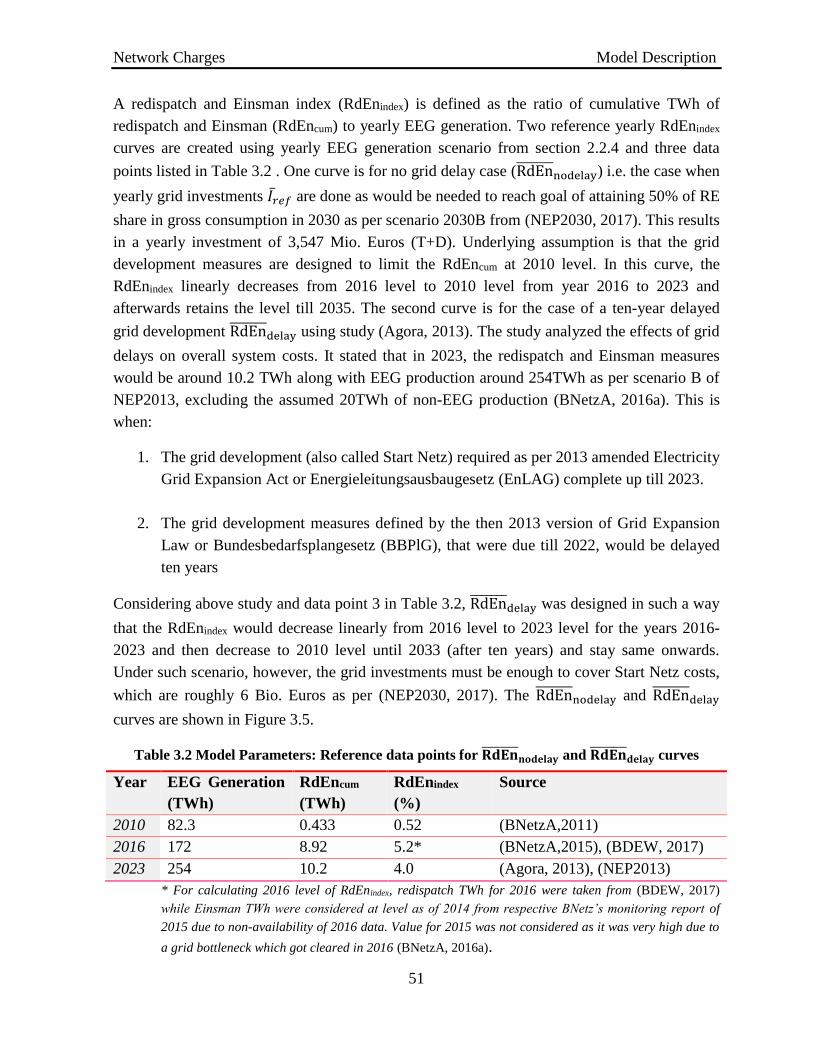
Network Charges Model Description
51
A redispatch and Einsman index (RdEnindex) is defined as the ratio of cumulative TWh of
redispatch and Einsman (RdEncum) to yearly EEG generation. Two reference yearly RdEnindex
curves are created using yearly EEG generation scenario from section 2.2.4 and three data
points listed in Table 3.2 . One curve is for no grid delay case (RdEn̅̅ ̅̅ ̅̅ ̅nodelay) i.e. the case when
yearly grid investments 𝐼�̅�𝑒𝑓 are done as would be needed to reach goal of attaining 50% of RE
share in gross consumption in 2030 as per scenario 2030B from (NEP2030, 2017). This results
in a yearly investment of 3,547 Mio. Euros (T+D). Underlying assumption is that the grid
development measures are designed to limit the RdEncum at 2010 level. In this curve, the
RdEnindex linearly decreases from 2016 level to 2010 level from year 2016 to 2023 and
afterwards retains the level till 2035. The second curve is for the case of a ten-year delayed
grid development RdEn̅̅ ̅̅ ̅̅ ̅delay using study (Agora, 2013). The study analyzed the effects of grid
delays on overall system costs. It stated that in 2023, the redispatch and Einsman measures
would be around 10.2 TWh along with EEG production around 254TWh as per scenario B of
NEP2013, excluding the assumed 20TWh of non-EEG production (BNetzA, 2016a). This is
when:
1. The grid development (also called Start Netz) required as per 2013 amended Electricity
Grid Expansion Act or Energieleitungsausbaugesetz (EnLAG) complete up till 2023.
2. The grid development measures defined by the then 2013 version of Grid Expansion
Law or Bundesbedarfsplangesetz (BBPlG), that were due till 2022, would be delayed
ten years
Considering above study and data point 3 in Table 3.2, RdEn̅̅ ̅̅ ̅̅ ̅delay was designed in such a way
that the RdEnindex would decrease linearly from 2016 level to 2023 level for the years 2016-
2023 and then decrease to 2010 level until 2033 (after ten years) and stay same onwards.
Under such scenario, however, the grid investments must be enough to cover Start Netz costs,
which are roughly 6 Bio. Euros as per (NEP2030, 2017). The RdEn̅̅ ̅̅ ̅̅ ̅nodelay and RdEn̅̅ ̅̅ ̅̅ ̅
delay
curves are shown in Figure 3.5.
Table 3.2 Model Parameters: Reference data points for 𝐑𝐝𝐄𝐧̅̅ ̅̅ ̅̅ ̅̅𝐧𝐨𝐝𝐞𝐥𝐚𝐲 and 𝐑𝐝𝐄𝐧̅̅ ̅̅ ̅̅ ̅̅
𝐝𝐞𝐥𝐚𝐲 curves
Year EEG Generation
(TWh)
RdEncum
(TWh)
RdEnindex
(%)
Source
2010 82.3 0.433 0.52 (BNetzA,2011)
2016 172 8.92 5.2* (BNetzA,2015), (BDEW, 2017)
2023 254 10.2 4.0 (Agora, 2013), (NEP2013)
* For calculating 2016 level of RdEnindex, redispatch TWh for 2016 were taken from (BDEW, 2017)
while Einsman TWh were considered at level as of 2014 from respective BNetz’s monitoring report of
2015 due to non-availability of 2016 data. Value for 2015 was not considered as it was very high due to
a grid bottleneck which got cleared in 2016 (BNetzA, 2016a).

Network Charges Model Description
52
Figure 3.5 Model Parameter: 𝐑𝐝𝐄𝐧̅̅ ̅̅ ̅̅ ̅̅𝐧𝐨𝐝𝐞𝐥𝐚𝐲 and 𝐑𝐝𝐄𝐧̅̅ ̅̅ ̅̅ ̅̅
𝐝𝐞𝐥𝐚𝐲 curves
Once the RdEn̅̅ ̅̅ ̅̅ ̅nodelay and RdEn̅̅ ̅̅ ̅̅ ̅
delay curves are defined, the input RdEncum for any year ‘y’ is
determined by following equation:
𝑹𝒅𝑬𝒏𝒄𝒖𝒎(𝒚) = [𝐑𝐝𝐄𝐧̅̅ ̅̅ ̅̅ ̅̅𝐧𝐨𝐝𝐞𝐥𝐚𝐲(𝒚) + 𝒅𝒆𝒍𝒂𝒚𝒇𝒄𝒕𝒓×(𝐑𝐝𝐄𝐧̅̅ ̅̅ ̅̅ ̅̅
𝐝𝐞𝐥𝐚𝐲(𝒚) − 𝐑𝐝𝐄𝐧̅̅ ̅̅ ̅̅ ̅̅𝐧𝐨𝐝𝐞𝐥𝐚𝐲(𝒚))]×𝑬𝑬𝑮 𝑮𝒆𝒏𝒆𝒓𝒂𝒕𝒊𝒐𝒏(y) (14)
Where the delayfctr ranges from 0 to 1 for delay in grid investments from 0 to 10 years. The
delay in grid investments is determined by subtracting cumulative scenario investment of the
year ‘y’ from cumulative 𝐼�̅�𝑒𝑓 and dividing it by 3,547 which is the reference yearly
investment for grid development without delay described before. Figure 3.6 shows the upper
and lower RdEncum curves for corresponding 10-year delay and no delay cases.
Figure 3.6 Model Scenario: Yearly RdEncum as per two curves 𝐑𝐝𝐄𝐧̅̅ ̅̅ ̅̅ ̅̅𝐝𝐞𝐥𝐚𝐲 and 𝐑𝐝𝐄𝐧̅̅ ̅̅ ̅̅ ̅̅
𝐧𝐨𝐝𝐞𝐥𝐚𝐲

Network Charges Model Results and Validation
53
3.2.4 Scenario for grid investments
It is already mentioned in section 2.2.3 that the future EEG plant development has been
assumed in line with scenario-2035B of (NEP2030, 2017). As per the said scenario, the RE
share in gross consumption is targeted at average 57% or an increase of 25.3% from status quo
31.7% RE share in 2015. Therefore, the yearly grid investments are determined as per
methodology presented in sections 3.2.1 and 3.2.2 by setting RE target of 57%. Yearly
investment, thus, come out as 4,393 Mio. Euros (T+D). Figure 3.7 shows that the cumulative
transmission and distribution investments for period 2015-2035 comes out around 56.4 and
31.4 Bio. Euros respectively. The figure also shows the trend of cumulative investments
needed against any targeted RE share increase. The trends show steeper increase as we target
higher increase of RE share in gross consumption.
Figure 3.7 Model Scenario: RE target share in gross consumption by 2035 and required
cumulative investments in Transmission and Distribution grid
3.3 Model Results and Validation
Figure 3.8 shows the model results for yearly transmission costs segregated into respective
components. A validation has been done for the model results with the prediction done by
(Hinz, et al., 2015) for 2024 transmission costs. The reference study assumed around 24.6 Bio.
Euros of cumulative transmission expansion investments in period 2015-2024 which is
comparable to this model’s assumed cumulative transmission investment of 25.3 Bio. Euros
for the same period. Model results indicate the transmission costs of 2024 as 6.3 Bio. Euros
against the reference study’s 6.4 Bio. Euros.
Figure 3.9 shows the model results for yearly distribution costs segregated into capital and
non-capital parts. A validation has been done for the model results with the prediction done by

Network Charges Model Results and Validation
54
(Hinz, et al., 2014) for 2023 distribution costs. The reference study assumed approximately
13.8 Bio. Euros of cumulative distribution expansion investments in period 2015-2023 which
is comparable to this model’s assumed cumulative distribution investment of 12.5 Bio. Euros
for the same period. Model results indicate the distribution costs of 2023 as 17.6 Bio. Euros
against the reference study’s 18.2 Bio. Euros.
Figure 3.8 Model Results: Yearly transmission costs vs 2024 transmission costs predicted by
(Hinz, et al., 2015)
Figure 3.9 Model Results: Yearly distribution costs vs 2023 distribution costs predicted by (Hinz,
et al., 2014)

Network Charges Model Results and Validation
55
Figure 3.10 shows the model results for average yearly network charges for household/SME
and unprivileged industry consumers. It is observable that there is a consistent increase in
charge levels from the year 2016 onwards. The network charges are slightly decreased from
2015 to 2016 due to low assumption taken about redispatch and Einsman costs. It can be
observed that network charges increase steeply for household/SME consumers as compared to
industrial consumers.
Figure 3.10 Model Results: Yearly average network charges for household/SME and industrial
(unprivileged) consumers
Appendix Table B.1 lists the yearly transmission, distribution and services costs while
Appendix Table B.2 presents the yearly average network charges for household/SME,
unprivileged industrial consumers and StromNEV-19 surcharges against categories A, B and
C. For OHU and AbLaV surcharges, as mentioned earlier in section 3.2, the associated total
costs are assumed constant, at level as of 2017, for the future years under this study scope.
OHU surcharge for categories A, B and C, thus, remains at levels of 0.058, 0.049 and 0.025
Cents/kWh respectively. AbLaV surcharge remains at level of 0.007 Cents/kWh.

KWKG Surcharge Perspective
56
4 KWKG SURCHARGE
4.1 Perspective
In Germany, since 1st April-2002 after coming into force of Combined Heat and Power Law or
Kraft-Wärme-Kopplung Gesetz (KWKG), KWK plants are supported through an independent
mechanism closely similar to EEG support system. Eligible KWK plants are generally offered
an optional guaranteed selling tariff based on past quarter’s average whole sale electricity
price along with fixed bonuses per unit of electricity generated in KWK mode. Some
payments are also directed to heat networks and storage providers. To find the specific portion
of electricity generated in KWK mode, a KWK rating factor is determined for each plant
through testing, that when multiplied to total heat produced gives the total KWK-electricity
eligible for support. For smaller installations with no heat meters, all produced electricity is
considered as KWK-electricity. Total costs of KWK support are recovered from consumers
through a special surcharge known as KWKG surcharge. Like EEG surcharge, certain
consumers are eligible to exemptions which is recovered by higher surcharge for unprivileged.
KWKG-2002 was very limited in its application and complexity. The support plan was offered
only for certain specific years and for plant categories differentiated as old, recent old or
modernized existing plants, new small plants below 2MW and fuel cell based plants. EEG
supported KWK plants were not given any support under this framework. Self-consumption or
use within private network e.g. within a building apartments was not eligible for support. The
support was given in fixed cents per kWh of eligible portion of production and yearly total
support was capped at 750Mio Euros.
KWKG was amended further in 2009 which led to inclusion of following important support
scheme changes:
1. Support of existing and new high efficiency KWK plants below 50KW or fuel cell
based plants were set to highest and was available for ten years.
2. For new KWK plants, high efficiency requirement was set in place along with support
either for period of 6 years or till 30,000 full load hours. Modernized high efficiency
plants were considered as new. Support was differentiated in capacity ranges like EEG.
3. Self-consumption was allowed a full support as the grid fed electricity.
Amendment of KWKG in 2012 brought a further change whereby along with modernized
plants, retrofitted power plants above 2MW were eligible for support. Support period
depended on costs related with such modernizations/retrofitting and was between 30,000 and
10,000 full load hours or as other option, if applicable, either 10 or 5 years.

KWKG Surcharge Model Description
57
Latest amendment of KWKG in 2016 brought along some fundamental changes and eligibility
conditions. Main additions are:
1. Coal based KWK plants are no more supported and transition from coal to other fuel
sources is encouraged through bonus over basic support. Bonus is also given to support
emission obligations of new power plants.
2. Yearly support cap was doubled and eligible full load hours for below 50MW KWK
plants was raised from 30,000 to 60,000 hours along with a general increase in support
prices in context to lowering wholesale prices which affected revenues of KWK plants
owing to their usual market price based agreements (Gailfuss, 2016). At the same time,
eligibility for support of self-consumption was limited to either small plants below
100KW or plants feeding energy intensive enterprises.
3. Micro KWK plants can either get per kWh support or a onetime payment at start.
4. Unlike previous KWKG versions, KWKG-2016 set a future goal in absolute terms i.e.
110 and 120TWh KWK based electricity by 2020 and 2025 respectively.
5. A reduced KWKG surcharge for railway industry of maximum either 0.03 or 0.04
cents/kWh was previsioned. KWK-surcharge will also be reduced for industries in
general in accordance to mechanism put in §64 of EEG (mentioned in 2.1.8) except
that it must not be below 0.03 cents/kWh.
4.2 Model Description
As already mentioned, that there are several exemptions and reductions allowed to KWKG
surcharge based on consumer category and nature. The developed model determines the base
KWKG surcharge for unprivileged consumers for a target year by following formula:
𝐾𝑊𝐾𝑠𝑢𝑟𝑐ℎ𝑎𝑟𝑔𝑒 =𝐶𝐾𝑊𝐾×𝑓𝑐𝑜𝑠𝑡
𝐶𝑜𝑛×𝑓𝑢𝑛𝑝𝑟𝑣 (15)
Where:
CKWK = Total KWKG costs for target year
Con= Consumption in target year (assumed same for all years as of 2015)
fcost= Factor to determine amount of CKWK left after excluding revenues from privileged consumers
funprv=Factor to determine amount of Con left after excluding privileged consumption
(fcost and funprv are determined as 0.978 and 0.540 using 2017 prognose (TSOs, 2016c) while Con is set
to 488TWh as of 2015. All parameters are assumed non-variable for calculations of future years)

KWKG Surcharge Model Description
58
Removing cost and consumptions factors from equation (15) and using 80% or 85 %
reductions, KWK surcharge for 20% and 15% categories of privileged industries (mentioned
in 2.1.8) can be determined respectively. CKWK for a target year is a sum of three main
elements provisioned in KWKG-2016:
𝐶𝐾𝑊𝐾 = 𝐶𝑠𝑢𝑝𝑝𝑜𝑟𝑡 + 𝐶𝑜𝑛𝑒𝑡𝑖𝑚𝑒𝑝𝑎𝑦𝑚𝑒𝑛𝑡 + 𝐶𝑛𝑒𝑡/𝑠𝑡𝑜𝑟𝑎𝑔𝑒 (16)
Where:
Csupport = Costs owing to payment in cents/kWh to KWK generation
Conetimepayment= Costs owing to onetime payment option for less than 2KW KWK plants
Cnet/storage= Costs owing to payments to heat networks and heat storage systems
Two cost components, Conetimepayment and Cnet/storage, made less than 10% of total KWKG costs
in recent several years. They are assumed at the levels as of 2016 as per (TSOs, 2016c). Csupport
is calculated through detailed modeling. Csupport is the total costs accounted for paying support
in cents/kWh to eligible KWK plants for KWK-generation as per terms and conditions of
KWKG applicable in the period when the plant got commissioned. To estimate these costs, it
is therefore essential to handle separately the different KWKG regimes of 2009, 2012 and
2016. Based on limited data availability and relative size of KWKG surcharge component in
overall electricity costs, a simple approach is adopted whereby Csupport is estimated for the
target year by following formula:
𝐶𝑠𝑢𝑝𝑝𝑜𝑟𝑡 = ∑ (𝐶𝑎𝑝2009×𝑃2009 + 𝐶𝑎𝑝2012×𝑃2012 + 𝐶𝑎𝑝2016×𝑃2016)×𝐶𝐹
𝐶1,𝐶2,𝐶3,𝑀
(17)
Where:
M, C1, C2, C3= plant categories explained below
Cap= Cumulative capacity per category till target year falling under KWKG-2009/2012/2016
CF= Capacity factor per category
P= Average per unit support payments per category falling under KWKG-2009/2012/2016
For calculating Cap2009,2012,2016, a data set is taken from (Öko-Institut, 2015), shown in
Appendix Table C.1, which contained the yearly additional capacities in MWs that came
under the KWKG support from 2009 till 2014. The data set is modified into four categories.
Three categories are for new, replaced or retrofitted KWK plants based on capacity sizes i.e.
C3 for less than 50KW, C2 for 50-2000KW and C1 for above 2MW. Category-M is for
modernized plant capacities falling in all size ranges. From the dataset, expiring capacities and
corresponding years are determined based on incoming capacity timelines and an average
support period estimate per category. Cap2009,2012,2016 is determined by summing the yearly
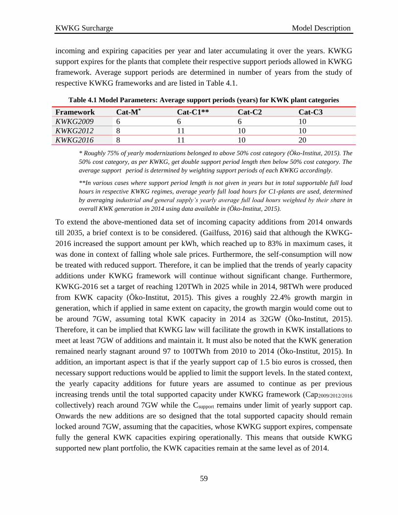
KWKG Surcharge Model Description
59
incoming and expiring capacities per year and later accumulating it over the years. KWKG
support expires for the plants that complete their respective support periods allowed in KWKG
framework. Average support periods are determined in number of years from the study of
respective KWKG frameworks and are listed in Table 4.1.
Table 4.1 Model Parameters: Average support periods (years) for KWK plant categories
Framework Cat-M* Cat-C1** Cat-C2 Cat-C3
KWKG2009 6 6 6 10
KWKG2012 8 11 10 10
KWKG2016 8 11 10 20
* Roughly 75% of yearly modernizations belonged to above 50% cost category (Öko-Institut, 2015). The
50% cost category, as per KWKG, get double support period length then below 50% cost category. The
average support period is determined by weighting support periods of each KWKG accordingly.
**In various cases where support period length is not given in years but in total supportable full load
hours in respective KWKG regimes, average yearly full load hours for C1-plants are used, determined
by averaging industrial and general supply’s yearly average full load hours weighted by their share in
overall KWK generation in 2014 using data available in (Öko-Institut, 2015).
To extend the above-mentioned data set of incoming capacity additions from 2014 onwards
till 2035, a brief context is to be considered. (Gailfuss, 2016) said that although the KWKG-
2016 increased the support amount per kWh, which reached up to 83% in maximum cases, it
was done in context of falling whole sale prices. Furthermore, the self-consumption will now
be treated with reduced support. Therefore, it can be implied that the trends of yearly capacity
additions under KWKG framework will continue without significant change. Furthermore,
KWKG-2016 set a target of reaching 120TWh in 2025 while in 2014, 98TWh were produced
from KWK capacity (Öko-Institut, 2015). This gives a roughly 22.4% growth margin in
generation, which if applied in same extent on capacity, the growth margin would come out to
be around 7GW, assuming total KWK capacity in 2014 as 32GW (Öko-Institut, 2015).
Therefore, it can be implied that KWKG law will facilitate the growth in KWK installations to
meet at least 7GW of additions and maintain it. It must also be noted that the KWK generation
remained nearly stagnant around 97 to 100TWh from 2010 to 2014 (Öko-Institut, 2015). In
addition, an important aspect is that if the yearly support cap of 1.5 bio euros is crossed, then
necessary support reductions would be applied to limit the support levels. In the stated context,
the yearly capacity additions for future years are assumed to continue as per previous
increasing trends until the total supported capacity under KWKG framework (Cap2009/2012/2016
collectively) reach around 7GW while the Csupport remains under limit of yearly support cap.
Onwards the new additions are so designed that the total supported capacity should remain
locked around 7GW, assuming that the capacities, whose KWKG support expires, compensate
fully the general KWK capacities expiring operationally. This means that outside KWKG
supported new plant portfolio, the KWK capacities remain at the same level as of 2014.

KWKG Surcharge Model Description
60
Figure 4.1shows the input scenario of category wise yearly accumulated capacities (regardless
of individual KWKG frameworks) along with the actual new capacities obtained by summing
categories C1, C2 and C3. It can be observed that installed capacity under all categories,
except M, become stagnant after 2018 upon reaching the newly supported total capacity of
7000MW. Installed capacities under category M saturates after 2020 as the further increase
would cause CKWK to cross yearly cap.
Figure 4.1 Model Scenario: Yearly accumulated capacities for categories M, C1, C2, C3 and new
KWK capacity obtained from summing C1, C2 and C3 results.
The parameters P and CF, used in equation (17), are plant dependent. However, due to
absence of plant based dataset, average values are estimated. CF is determined from
accumulated installed KWKG capacity as described earlier and KWKG eligible generation
taken from ‘Jahresabrechnung’ report of year 2014 (TSOs, 2015) and is listed in Table 4.2.
Figure 4.2 shows the actual variations of capacity factor over the period of 2013-2015. It can
be observed that setting the capacity factors at the values observed in 2015 is roughly justified
since the variation over the past two years are not very significant. The parameter set P which
feature the average payments in cents/kWh to KWK plants per category and per KWKG
regime is also determined using ‘Jahresabrechnung’ reports and is shown in Table 4.2. For
KWKG-2009 & 2012, Jahresabrechnung reports of 2011 (TSOs, 2012) and 2014 (TSOs,
2015) are used respectively. These years are chosen in such a manner that tail effects of
KWKG 2002 regime in 2009 & 2010 and transition effects of KWKG2009 and KWKG2012
in year 2012 can be avoided. Years 2013 and 2014 are also skipped since year 2015 provides
the latest figures. For calculating average P values per category for KWKG2012 using year
2015, total yearly payments are first subtracted with payments owing to plants falling under

KWKG Surcharge Model Results and Validation
61
KWKG2009. The flexibility of choosing a specific year is justified since unlike EEG
framework, remuneration rates do not change under KWKG frameworks. P values for
KWKG2016 are not possible to estimate in same fashion since no data is yet available. They
are set at 50% increase from past values based on a broad approximation of results obtained by
comparing support sets of C1, C2 and C3 classes for KWKG 2016 & 2012 using plant
capacities in range of 1KW-50MW.
Table 4.2 Model Parameters: P(cents/kWh) and CF for KWK plants
Parameter Cat-M Cat-C1 Cat-C2 Cat-C3
P2009 1.68 1.59 2.45 5.11
P2012 2.20 2.28 3.46 5.41
P2016 3.3 3.42 5.19 8.11
CF 0.36 0.29 0.4 0.51
Figure 4.2 Variation of KWK capacity factors over 2013-2015
4.3 Model Results and Validation
Figure 4.3 shows the results of the model calculation of yearly KWK support costs occurring
per plant category. The model calculations follow in general the trends seen in past years. The
costs prediction of 2017 provided by (TSOs, 2016c) aligns well with the model results. Figure
4.4 gives the future trend of base KWKG surcharge for unprivileged consumers as per
KWKG-2016 mechanism, mentioned by equation (15). Appendix Table C.2, provides the
aggregate yearly installed capacities, generation, costs and KWKG surcharge values as
resulted from model calculations.

KWKG Surcharge Model Results and Validation
62
Figure 4.3 Model Results: Yearly KWK support costs plotted along with known support costs as
per Jahresabrechnungen reports of 2009-2015 and 2017 prognose (TSOs, 2016c).
Figure 4.4 Model Results: Yearly base KWK surcharge for unprivileged consumers as per
KWKG-2016 mechanism

Price development till 2035 Household Consumption
63
5 PRICE DEVELOPMENT TILL 2035 Results from the prior described python models are segregated as per applicable regulations,
across three consumption classes defined in next sections along with model results. In the
yearly results, the components; billing/metering & operation fees, concession fees, electricity
duty and supply costs are assumed to remain at same level as of 2015, shown in Table 1.2. The
results are presented excluding VAT component.
5.1 Household Consumption
Households are connected to the grid at low voltage (0.4KV). Households are metered on non-
interval basis using standard load profile and are not considered for any exemptions in
network charges as discussed in 3.1.6. Households generally consume less than 10,000kWh
which makes them in-eligible to any reductions in surcharges or electricity duty. Figure 5.1
shows the model results for the yearly average electricity price development of household
customers. The results show that household would face an increase of roughly 3.37
Cents/kWh in electricity prices till 2028 mainly due to rising EEG surcharge and network
charges. After 2028, the falling EEG surcharge levels would provide some relief but the prices
would still be higher than 2015 due to consistently increasing network charges.
Figure 5.1 Yearly average electricity price development for household customers from model
calculations (Values for 2013,2014 from BNetzA)
5.2 Unprivileged Industrial Consumption
An unprivileged industry would be the one which is not linked to rail system and which is
connected to high or medium voltage grid system (110KV or 35KV). The yearly consumption

Price development till 2035 Privileged Industrial Consumption
64
for such industry would generally lie above 24GWh as per (BNetzA, 2016a), however, as per
category scope only the costs of the first GWh consumption are considered. Therefore, no
reductions in EEG, KWKG, StromNEV-19 and OHU Surcharges are applicable. Owing to
connection to high voltage network, such industry enjoys significantly reduced network
charges and concession fees. However, it is assumed that the industry does not qualify for any
reductions in network charges owing to its asymmetric load profile. Due to high consumption
volumes, the billing/metering costs and supply costs are also relatively less for industries.
Figure 5.2 shows the yearly price development for this consumption category. The results
show an increase of roughly 2.17 Cents/kWh in electricity prices till 2024.
Figure 5.2 Yearly average electricity price development for unprivileged industrial consumption
from model calculations (Values for 2013,2014 from BNetzA)
5.3 Privileged Industrial Consumption
For privileged consumption class, an industrial load similar to one described in previous
section can be considered with assumption that industry’s electricity cost intensity, described
in section 2.1.8, is at least 20% and consumption class considered is above 1GWh so that it is
eligible for 85% reduction in EEG and KWKG surcharge as per §64-EEG-2017 and qualify
for category C rate in regard to application of StromNEV-19 and OHU surcharge. It is also
assumed that the industry has asymmetric load with full load hours above 8000 hours so that it
gets only 10% of regular network charges. It is further assumed that the said consumption
class relates to those manufacturing processes which are exempt from electricity duty. This
legal provision is in place to safeguard international competitiveness of German industry.
Figure 5.3 shows the yearly price development for said consumption category. The results
show that said consumption class would face a minute increase of roughly 0.24 cents/kWh in
electricity prices till 2024.

Price development till 2035 Privileged Industrial Consumption
65
Figure 5.3 Yearly average electricity price development for privileged industrial consumption
from model calculations (Values for 2013,2014 from BNetzA)
Figure 5.4 depicts the five-yearly electricity retail price development across three consumption
classes discussed above. It can be observed that the relative increase of component prices,
resulted from model predications, is highest for the household consumers and there is hardly
any such effect observable for privileged industrial consumption.
Figure 5.4 Five yearly electricity price development for three consumption classes; Households
(Left), unprivileged industry (middle) and privileged industry (right)

Conclusion & Outlook Integration of RE generation
66
6 CONCLUSION & OUTLOOK Two important aspects are clearly visible from model results. Firstly, the EEG energy
generation will rise significantly till 2035, which would make roughly 60% increase from
status quo level of 2015. Secondly, the retail electricity prices are still expected to rise owing
to increasing EEG surcharge and network charges. The integration of fast growing renewable
energy generation and rising retail prices within Germany, are already the subjects of intense
discussion on diverse social, political, economic and academic forums. The next two sub
sections give a brief outlook on these subjects in light of several consulted literatures. The last
subsection presents the existing model research gaps and outlook of the future research
possibilities to enhance the developed python models.
6.1 Integration of RE generation
Fast RE growth has already revolutionized the German electricity industry. RE growth has
made whole sale electricity prices to fall considerably not only within Germany but also in
neighboring countries. It has noticeably contributed towards reducing country’s dependency
on imported fuels. Vast spread decentralized solar generation has brought a strong prosumer
culture at the end user side of the electricity supply chain. The efforts for smart grids and
digitalization make more sense now and are happening with clear directions. The variable RE
generators are participating in reserve markets using spatial diversity benefits, thus,
unshackling the core limitation of variability of individual RE installations through
cooperation. On the other hand, RE growth has brought grid development challenges to cope
with redispatch and Einsman costs. Electricity markets are facing critical challenge to
maintain long term supply security nationally and on European level.
Integration of RE generation is not a solo pursuit of Germany. It’s a collective European
ambition as well. (Agora, 2015) states that 70% of EU’s new electricity installations of 2013
were RE based. The author illustrated Germany’s standings in the 2020-RE targets across EU
member states, shown in Figure 6.1. The figure shows clearly that Germany’s RE ambition
aligns well into EU context. In such environments, the author states that the close cooperation
of cross border electric grids can improve the supply security in concern to rising RE
generation. As per new methods developed by Pentalateral Energy Forum for joint assessment
of resource adequacy, the author states that joint peak load of EU neighbors comes out 10GW
lesser than the sum of individual country load peaks. However, this close cooperation has yet
to meet many challenges.
(Stefes & Hagor, 2016) states that the need for grid development in Germany had already been
identified by German Energy Agency (Dena) in 2005. However, the political, financial and
administrative limitations delayed the process. In the meantime, cross border EU

Conclusion & Outlook Integration of RE generation
67
interconnections helped meeting the north based high generation and south based high
consumption of Germany. In recent years, grid congestion from German north to south has
caused electricity produced from RE installations of north, to take indirect paths, also called
loop flows, through east European countries like Poland, Czech, Slovakia and Hungary
(Schlandt, 2015). The loop flows compromised the N-1 grid security criteria of the affected
countries. Complains from these countries led to the installation of physical power controlling
devices at some grid points which made it even more important to pursue grid development to
cope with expected high growth of RE in north, especially offshore wind.
Figure 6.1 EU 2020-RE targets [Taken from (Agora, 2015)]
Rapidly increasing RE generation is also a matter of concern as present electricity markets
provide insufficient price signals and incentives to encourage flexible but expensive peak
power plants and baseload generators, that lack flexibility to tune to cheap variable RE feed in,
to stay in operation. For future, Germany is favoring for a market only approach supported by
strategic reserves, however, other European countries favor capacity markets as evident from
the recent Winter Package from EU Commission. If Germany, would take a solo path, it may
end up with disadvantages on national and EU level as investigated by (Statnett, 2015). The
author states that such a path would lead Germany to depend more on electricity imports at the
time of low RE generation. This would also lead neighboring countries to focus strongly on
capacity security due to lack of any investment signals from Germany.
By far, Germany has been very successful in bringing the positive effects of Energiewende in
electricity sector. However, with the expanded RE portfolio, the need for sector coupling has
become much more important. Electric vehicles, electricity storage, demand side management,
power to heat etc. are the options that must be promoted to cope with future periods of peak or
no RE generation when the backup would be either insufficient or too expensive to afford.

Conclusion & Outlook Rising retail electricity prices
68
6.2 Rising retail electricity prices
Rising retail electricity prices have already been a big concern for Germany despite the
benefits of RE energy sales at the wholesale market level. Apart from the rising EEG costs,
regional problems with network charges are also present. Consumers of DSOs that are facing
high decentralized RE growth, are paying for increased costs owing to avoided network
charges that relieve, in turn, the EEG surcharge levels for all country. Region based network
charges are rising for less dense German north due to grid expansions for offshore RE
installations and general reinforcements to cope with decentralized RE generation.
Rising EEG surcharge levels have already changed the course of EEG when in 2012, the solar
cap was introduced which was later extended to wind and biomass as well. In context to
developing EU context and to promote cost efficiency, auction system was also introduced in
EEG-2017. However, the EEG mechanism has not remained simple anymore and there is a
strong counter pulling argument. Controlling the cost efficiency may contradict with the
fundamental Energiewende dimension of diversified ownership. (Stefes & Hagor, 2016)
suggests that the introduction of auction system may reverse the trend of decentralized RE
plant ownerships back to big investors as they can easily outcompete the former in energy
costs. It was due to such concerns, EEG-2017 provisioned no auctions for below 750 KW
solar and wind plants and below 150KW biomass plants.
Exemptions allowed in EEG mechanism is also a great social debate in Germany. (Agora,
2015) states that although the household electricity retail prices in Germany are relatively
high, the average household consumption is quiet small which ends up in same energy
expenses as the households of comparable industrialized countries. However, (Stefes & Hagor,
2016) states that Energiewende is socially unbalanced, which distributes income from bottom
to middle and top class. The author argues that industries enjoy EEG exemptions and the
lower wholesale electricity prices due to Energiewende. The home owners and farmers pay
higher electricity bills but they also benefit from own RE generation. Those who live in
apartments face the high electricity costs but counter some effects through efficient use of
electricity. However, the lowest income class may not even utilize the efficiency measures due
to insufficient savings to invest. (Ecofys, 2015) states that energy intense German industries,
that receive full privileges on surcharges/electricity duty and reduced grid fees, get
competitive electricity rates. Without such privileges, the German households and small
businesses may enjoy slightly reduced EEG surcharges (around 1.6 cents as of 2014).
However, lack of privileges would have negative macroeconomic effects along with around
104,000 lost jobs, estimated by the authors.

Conclusion & Outlook Research gaps and future research direction
69
6.3 Research gaps and future research direction
During the development of the models for EEG, KWKG, StromNEV-19 surcharges and
network charges, some key research gaps were either deliberately simplified or could not be
modelled due to time constraints. The brief description of these research gaps is listed below:
1. All Models: A constant yearly consumption has been assumed for future years. Yearly
consumption depends on several factors such as economic conditions, efficiency
incentives, demographic changes etc. A research can be conducted to develop a more
realistic consumption scenario. Furthermore, the factors used in equations (1), (8), (9),
(10) and (15) depend on yearly consumption trends between privileged and
unprivileged consumers. At present these factors are simply assumed based on forecast
results from (TSOs, 2016a), (Hinz, et al., 2015) and (TSOs, 2016c). In future, the
model can be enhanced to model privileged and unprivileged consumptions and cost
distributions.
2. EEG Model: Future development of EEG average tariffs was estimated using (Oeko-
Institut, 2016) with simple linear interpolation. In practice, these tariffs depend on
several aspects such as learning curve effects, technical improvements, social
acceptance etc. A research can be conducted to develop a more realistic future tariff
scenario by incorporating above stated aspects.
3. EEG Model: To get rid of underestimation of costs for wind onshore plants owing to
assumption of the same minimum initial tariff period of 5 years, an average increase of
9 years was added to all onshore plants, based on weighted average initial tariff periods
of country wide wind plants on lands with varying wind resource potentials, as
described in 2.2.2. This approach is an oversimplification of EEG costs for the wind
onshore plants. In future, model can be enhanced in such a fashion that the wind
onshore plants available in the plant database (Energymap, 2017) can be given
individual initial tariff periods based on their geographical parameters i.e. Nuts3 or
Merra2 ids.
4. EEG Model: At present a single cleavage strategy is assumed for distributing market
factors among smaller and bigger plants. In future, model can be enhanced to feature
three or more plant groupings with distinct direct marketing habits as evident from
illustrations provided by (Götz, et al., 2013).
5. Network Charges Model: The relation between needed grid investments and targeted
RE shares was estimated using two data points each of distribution and transmission
sectors. Although, the original target was to collect at least four data points for each
sector to achieve higher accuracy of predictions, author’s limited ability with literature

Conclusion & Outlook Research gaps and future research direction
70
research in German language, hindered the progress and confined the research to two
points each only. In future, this aspect can be enhanced relatively easily by further
research of additional data points.
6. Network Charges Model: The model does not incorporate the detailed modeling of
avoided network charges. The sharp rise of costs incurred by DSOs in respect of
avoided network charges, in recent past, has already sparked huge debate in academic
researches. In future, the model can be enhanced to incorporate modeling of costs of
avoided network charges. It will enable the model users to conduct researches on better
policy options for handling such costs.
7. KWKG Model: The support rates per kWh for KWK generation as per KWKG-2016
was assumed as 150% of KWKG-2012 rates based on a broad approximation of results
obtained by comparing support sets of C1, C2 and C3 classes for KWKG 2016 & 2012
using plant capacities in range of 1KW-50MW. This approximation was adopted due
to absence of data i.e. the Jahresabrechnung report-2016 for KWKG yearly accounts
has not been yet published. Upon the availability of the said and additional data, the
average support rates can be appropriately researched and incorporated.
As already shortly discussed in the subsection 6.2 that the rising retail electricity prices are
sparking strong social concerns in Germany. Model results for EEG surcharge and network
charges predict further increase in prices in future which are significant enough to be
considered. Consequently, these results drive the motivation for a possible research into
analyzing effects of opting innovative policy options that would dampen the increasing prices
partially. However, such researches can only be realistically conducted if further models are
integrated with the developed model. These further models may include the modeling of future
developments of wholesale electricity prices, yearly supply margins, yearly consumption,
feedback effects of electricity prices on consumption behaviors etc.
References
71
REFERENCES
Agora, 2013. Cost Optimal Expansion of Renewables in Germany: A comparison of strategies
for expanding wind and solar power in Germany, Berlin: Agora Energiewende.
Agora, 2014. Vergütung von Windenergieanlagen an Land über das Referenzertragsmodell,
Berlin: Agora Energiewende.
Agora, 2015. Understanding the Energiewende: FAQ on the ongoing transition of the German
power system, Berlin: Agora Energiewende.
Agora, 2016. Energiewende: What do the new laws mean? Ten questions and answers about
EEG 2017, the Electricity Market Act, and the Digitization Act, Berlin: Agora Energiewende.
Bayer, E., 2015. Report on German Power System, Berlin: Agora Energiewende.
BDEW, 2010. Prognosen zur Entwicklung der Stromversorgung und Einordnung der
Energieszenarien für ein Energiekonzept der Bundesregierung, Berlin: Bundesverband der
Energie- und Wasserwirtschaft e.V..
BDEW, 2017. Redispatch in Deutschland, Berlin: Bundesverband der Energie- und
Wasserwirtschaft e.V..
Behringer, J. M., 2016. Distribution networks for the energy transition: Legal framework and
practical experience. [Online] Available at: http://enr-ee.com/de/veranstaltungen/leser/
konferenz-zu-verteilnetze-fuer-die-energiewende.html [Accessed 01 05 2017].
BMWi, 2016a. 2017 Revision of Renewable Energies Sources Act: Key points of the decision
by the German Bundestag of 8 July 2016. [Online] Available at: http://www.bmwi.de/
Redaktion/EN/Downloads/eeg-novelle-2017-praesentation.html [Accessed 14 05 2017].
BMWi, 2016b. EEG in Zahlen: Vergütungen, Differenzkosten und EEG-Umlage 2000 bis
2017, Berlin: Bundesministerium für Wirtschaft und Energie.
BNetzA, 2016a. Monitoringbericht, s.l.: Bundesnetzagentur.
BNetzA, 2016b. EEG in Zahlen 2015, s.l.: Bundesnetzagentur.
BNetzA, 2017. The main tools of incentive regulation in Germany. [Online] Available at:
https://www.bundesnetzagentur.de/EN/Areas/Energy/Companies/GeneralInformationOnEnerg
yRegulation/IncentiveRegulation/Tools/IncentReg_Tools-node.html [Accessed 15 05 2017].

References
72
Brandt, T., 2006. Liberalisation, privatisation and regulation in the German electricity sector,
Düsseldorf: Wirtschafts- und Sozialwissenschaftliches Institut (WSI) in der Hans-Böckler-
Stiftung.
Dena-Netzstudie II, 2010. Integration erneuerbarer Energien in die deutsche
Stromversorgung im Zeitraum 2015 – 2020 mit Ausblick 2025., Berlin: Deutsch Energie-
Agentur.
Dena-Verteilnetzstudie, 2012. Ausbau und Inovationsbedarf der Stromverteilnetze in
deutschland bis 2030, Berlin: Deutsche Energie-Agentur.
Ecofys, 2014. Development of a retrofit program for distributed generation in Germany for
the prevention of frequency stability problems in abnormal system conditions, s.l.: BMWi
Germany.
Ecofys, 2015. Electricity Costs of Energy Intensive Industries: An International Comparison,
Berlin: BMWi.
Energymap, 2017. EEG plants data base of Germany, s.l.: Energymap.info.
Gailfuss, M., 2016. Germany's new CHP Act explained. Decentralized energy.
Geipel, M., 2014. The Amended Renewable Energy Sources Act 2014 (EEG). Berlin: Noerr.
Götz, P., Huschke, T. & Lenck, T., 2013. Auswirkungen der verpflichtenden
Direktvermarktung für EEG-Neuanlagen, Berlin: Energy Brainpool.
Gründinger, W., 2017. Drivers of Energy Transition. 1 ed. Berlin: VS Verlag für
Sozialwissenschaften.
Hinz, F., Iglhaut, D., Frevel, T. & Möst, D., 2014. Abschätzung der Entwicklung der
Netznutzungsentgelte in Deutschland, Dresden: Technische Universität Dresden.
Hinz, F., Iglhaut, D., Frevel, T. & Möst, D., 2015. Abschätzung der Entwicklung der
Netznutzungsentgelte in Deutschland, Dresden: Technische Universität Dresden.
Hirth, L. & Ziegenhagen, I., 2013. Control power and variable renewables: A glimpse at
German data. Stockholm, IEEE.
IE Leipzig, 2012. Entwicklung der Preise für Strom und Erdgas in Baden-Württemberg bis
2020, Leipzig: Leipziger Institut für Energie GmbH.
Joskow, P. L., 2006. Regulation of the electricity market. DICE Report, I(2).
NEP2030, 2017. Netzentwicklungsplan 2030-1st draft, Berlin: BNetzA.

References
73
Netztransparenz, 2016. EEG-Vergütungskategorientabelle mit allen Kategorien bis
Inbetriebnahmejahr 2017. [Online] Available at: https://www.netztransparenz.de/
EEG/Verguetungs-und-Umlagekategorien [Accessed 24 02 2017].
netztransperenz, 2017. netztransperenz. [Online] Available at: www.netztransperenz.de
[Accessed 15 06 2017].
Oeko-Institut, 2016. Projected EEG Costs up to 2035, Berlin: A study commissioned by
Agora Energiewende.
Öko-Institut, 2015. Aktueller Stand der KWK-Erzeugung (Dezember 2015), Berlin: Öko-
Institut e.V..
Schlandt, J., 2015. Loops and cracks: Excess German power strains Europe’s grids. Clean
Energy Wire.
Statnett, 2015. A European Energy-Only Market in 2030, Oslo: Statnett.
Stefes, C. H. & Hagor, C., 2016. Germany’s Energy Transition: A Comparative Perspective.
1st ed. New York: Springer Nature.
TSOs, 2012. KWK-Gesetz / Jahresabrechnung 2011, Berlin: Netztransparenz.
TSOs, 2015. KWK-Gesetz / Jahresabrechnung 2014, Berlin: Netztransparenz.
TSOs, 2016a. Prognose der EEG-Umlage 2017 nach AusglMechV, Berlin: Netztransparenz.
TSOs, 2016b. Ermittlung der Umlage nach §19 Absatz 2 StromNEV in 2017 auf Netzentgelte
für Strommengen der Endverbrauchskategorien A, B und C, Berlin: Netztransparenz.
TSOs, 2016c. Prognose der indikativen KWKG-Umlage 2017 auf der Basis des
Regierungsentwurfs, Berlin: Netztransperenze.

Appendix A
74
Appendix A. Data relating to EEG Model
Appendix Table A.1 Model Scenario: Yearly EEG capacity (GWs) per technology
Year Biomass Geothermal Mine/Sewage/Landfill Gas
Solar Water Wind Offshore
Wind Onshore
2015 7.14 0.03 0.64 37.27 1.65 1.68 38.59
2016 7.15 0.03 0.64 37.40 1.65 3.65 39.71
2017 7.15 0.03 0.64 39.58 1.76 4.91 41.04
2018 7.15 0.03 0.64 41.76 1.88 6.17 42.38
2019 7.15 0.04 0.64 43.94 2.00 7.42 43.71
2020 6.89 0.03 0.46 46.11 2.12 8.68 41.52
2021 6.70 0.04 0.40 48.23 2.23 9.94 41.14
2022 6.71 0.04 0.42 50.15 2.42 10.55 42.64
2023 6.74 0.04 0.39 52.06 2.60 11.17 43.72
2024 6.69 0.04 0.36 53.93 2.79 11.78 45.14
2025 6.37 0.04 0.34 55.29 2.97 12.39 47.31
2026 5.88 0.04 0.39 56.39 3.16 13.01 49.55
2027 5.59 0.04 0.39 59.23 3.34 13.62 50.33
2028 5.42 0.04 0.39 61.64 3.53 14.24 51.54
2029 5.56 0.04 0.39 63.34 3.70 14.85 53.56
2030 5.65 0.03 0.39 62.62 3.40 15.43 53.79
2031 5.58 0.03 0.39 58.63 3.22 16.00 55.20
2032 4.97 0.04 0.38 57.71 3.21 16.81 57.02
2033 5.11 0.03 0.38 58.06 3.39 17.65 58.32
2034 5.28 0.02 0.39 62.15 3.60 18.22 58.95
2035 5.49 0.02 0.39 68.16 3.88 18.08 58.08
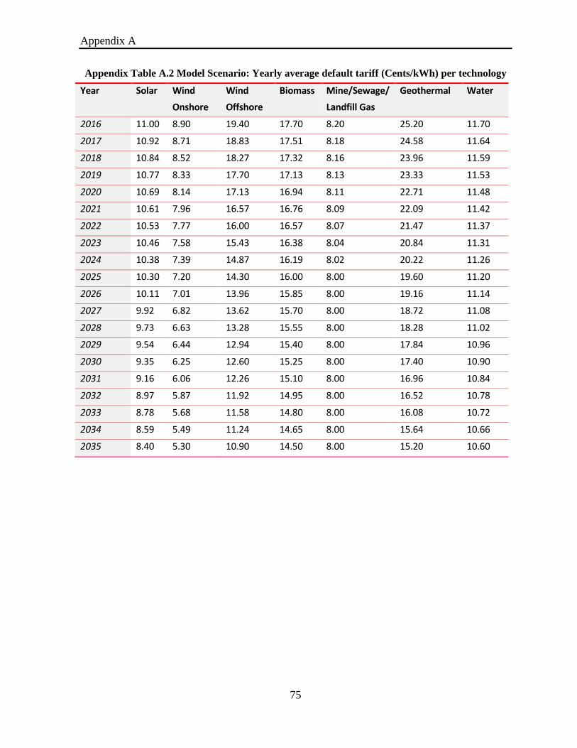
Appendix A
75
Appendix Table A.2 Model Scenario: Yearly average default tariff (Cents/kWh) per technology
Year Solar Wind
Onshore
Wind
Offshore
Biomass Mine/Sewage/
Landfill Gas
Geothermal Water
2016 11.00 8.90 19.40 17.70 8.20 25.20 11.70
2017 10.92 8.71 18.83 17.51 8.18 24.58 11.64
2018 10.84 8.52 18.27 17.32 8.16 23.96 11.59
2019 10.77 8.33 17.70 17.13 8.13 23.33 11.53
2020 10.69 8.14 17.13 16.94 8.11 22.71 11.48
2021 10.61 7.96 16.57 16.76 8.09 22.09 11.42
2022 10.53 7.77 16.00 16.57 8.07 21.47 11.37
2023 10.46 7.58 15.43 16.38 8.04 20.84 11.31
2024 10.38 7.39 14.87 16.19 8.02 20.22 11.26
2025 10.30 7.20 14.30 16.00 8.00 19.60 11.20
2026 10.11 7.01 13.96 15.85 8.00 19.16 11.14
2027 9.92 6.82 13.62 15.70 8.00 18.72 11.08
2028 9.73 6.63 13.28 15.55 8.00 18.28 11.02
2029 9.54 6.44 12.94 15.40 8.00 17.84 10.96
2030 9.35 6.25 12.60 15.25 8.00 17.40 10.90
2031 9.16 6.06 12.26 15.10 8.00 16.96 10.84
2032 8.97 5.87 11.92 14.95 8.00 16.52 10.78
2033 8.78 5.68 11.58 14.80 8.00 16.08 10.72
2034 8.59 5.49 11.24 14.65 8.00 15.64 10.66
2035 8.40 5.30 10.90 14.50 8.00 15.20 10.60

Appendix A
76
Appendix Table A.3 Model Scenario: Yearly EEG generation (TWh) per technology
Year Biomass Geothermal Mine/Sewage/Landfill Gas
Solar Water Wind Offshore
Wind Onshore
2015 40.62 0.13 1.42 34.88 5.28 12.56 70.10
2016 40.63 0.13 1.42 35.95 5.48 17.16 71.75
2017 40.63 0.14 1.42 37.95 5.86 21.53 73.88
2018 40.64 0.14 1.42 40.00 6.20 26.74 75.98
2019 40.64 0.14 1.42 42.04 6.59 30.92 77.99
2020 38.74 0.14 0.98 44.02 6.96 35.70 72.28
2021 38.27 0.14 0.91 45.91 7.42 39.26 73.19
2022 38.57 0.14 0.94 47.68 8.02 41.35 74.32
2023 38.64 0.15 0.85 49.47 8.64 43.71 75.91
2024 37.69 0.15 0.80 51.00 9.23 45.85 77.69
2025 36.03 0.15 0.84 52.19 9.85 48.28 81.35
2026 33.80 0.15 0.87 53.90 10.41 50.62 82.68
2027 32.07 0.15 0.87 56.65 11.02 52.84 83.58
2028 31.77 0.15 0.87 58.59 11.58 54.77 85.41
2029 32.62 0.14 0.87 59.68 11.91 57.31 86.59
2030 32.93 0.13 0.87 56.83 10.85 59.40 87.83
2031 31.76 0.14 0.86 56.17 10.38 61.60 90.53
2032 28.95 0.14 0.85 54.03 10.68 64.57 92.38
2033 30.00 0.07 0.86 56.15 11.31 66.89 93.50
2034 30.63 0.07 0.86 60.50 11.96 69.07 92.86
2035 32.39 0.06 0.87 67.04 13.02 63.21 91.68

Appendix A
77
Appendix Table A.4 Model Results: Yearly EEG surcharge (Cents/kWh) for privileged and
unprivileged consumer categories
Year EEG Surcharge
(15% Category)
EEG Surcharge
(20% Category)
EEG Surcharge
(Railways)
EEG Surcharge
(Unprivilaged)
2015 0.68 0.90 0.90 6.37
2016 0.70 0.93 0.93 6.60
2017 0.73 0.97 0.97 6.84
2018 0.75 1.00 1.00 7.09
2019 0.78 1.04 1.04 7.34
2020 0.79 1.05 1.05 7.44
2021 0.81 1.07 1.07 7.59
2022 0.82 1.09 1.09 7.72
2023 0.83 1.11 1.11 7.84
2024 0.83 1.11 1.11 7.82
2025 0.82 1.10 1.10 7.75
2026 0.81 1.08 1.08 7.62
2027 0.79 1.06 1.06 7.47
2028 0.78 1.04 1.04 7.32
2029 0.75 1.00 1.00 7.06
2030 0.69 0.92 0.92 6.48
2031 0.63 0.84 0.84 5.97
2032 0.56 0.74 0.74 5.25
2033 0.52 0.70 0.70 4.92
2034 0.54 0.71 0.71 5.05
2035 0.56 0.75 0.75 5.27

Appendix B
78
Appendix B. Data relating to Network Charges Model
Appendix Table B.1 Model Results: Yearly transmission, distribution, services costs and
aggregated network costs
Year Transmission Costs
(Mio. Euros)
Distribution Costs
(Mio. Euros)
Services Costs
(Mio. Euros)
Total Network Costs
(Bio. Euros)
2015 2895.98 15595.17 1399.51 19.89
2016 3227.93 15865.71 772.70 19.87
2017 3554.94 16130.87 737.44 20.42
2018 3876.99 16390.63 697.72 20.97
2019 4194.10 16645.00 649.70 21.49
2020 4506.26 16893.98 583.61 21.98
2021 4813.48 17137.56 524.99 22.48
2022 5115.74 17375.76 461.90 22.95
2023 5413.07 17608.56 394.92 23.42
2024 5705.44 17835.97 398.88 23.94
2025 5992.87 18057.99 403.18 24.45
2026 6275.35 18274.62 406.80 24.96
2027 6552.88 18485.86 410.69 25.45
2028 6825.47 18691.71 414.90 25.93
2029 7093.11 18892.16 419.12 26.40
2030 7355.80 19087.22 421.66 26.86
2031 7613.55 19276.90 424.98 27.32
2032 7866.35 19461.18 427.64 27.76
2033 8114.20 19640.07 432.17 28.19
2034 8357.10 19813.56 436.71 28.61
2035 8595.06 19981.67 439.95 29.02

Appendix B
79
Appendix Table B.2 Model Results: Yearly average network charges for household/SME,
unprivileged industry and StromNEV-19 surcharge for categories A, B, C in Cents/kWh
Year Network Charge
Household/SME
Network Charge
Unprevilaged
Industry
StromNEV-19
Surcharge
Category- A
StromNEV-19
Surcharge
Category-B
StromNEV-19
Surcharge
Category-C
2015 6.882 2.059 0.388 0.050 0.025
2016 6.873 2.057 0.387 0.050 0.025
2017 7.063 2.114 0.399 0.050 0.025
2018 7.248 2.169 0.411 0.050 0.025
2019 7.427 2.222 0.422 0.050 0.025
2020 7.596 2.273 0.432 0.050 0.025
2021 7.764 2.323 0.442 0.050 0.025
2022 7.927 2.372 0.452 0.050 0.025
2023 8.085 2.419 0.462 0.050 0.025
2024 8.263 2.473 0.473 0.050 0.025
2025 8.439 2.525 0.484 0.050 0.025
2026 8.610 2.576 0.495 0.050 0.025
2027 8.778 2.627 0.505 0.050 0.025
2028 8.943 2.676 0.515 0.050 0.025
2029 9.104 2.724 0.525 0.050 0.025
2030 9.261 2.771 0.535 0.050 0.025
2031 9.415 2.817 0.544 0.050 0.025
2032 9.565 2.862 0.554 0.050 0.025
2033 9.712 2.906 0.563 0.050 0.025
2034 9.856 2.949 0.572 0.050 0.025
2035 9.996 2.991 0.580 0.050 0.025

Appendix C
80
Appendix C. Data relating to KWKG model
Appendix Table C.1 Dataset from (Öko-Institut, 2015) featuring yearly additional capacities in
MWs coming under KWKG support mechanism categorized as per category M, C1, C2, C3
Year Cat-M Cat-C1 Cat-C2 Cat-C3
2009 94 260 115 55
2010 166 427 134 40
2011 23 335 173 52
2012 211 266 195 53
2013 796 295 242 62
2014 836 400 324 81
Appendix Table C.2 Model Results: Aggregated yearly installed capacities, generation, costs and
KWKG surcharge values as resulted from model calculations
Year Installed Capacity
(GW)
KWK Generation
(TWh)
Support Cost
(Mio. Euros)
Base KWKG-Surcharge
(Cents/kWh)
2017 10307 33 1047 0.3885
2018 12260 39 1239 0.4597
2019 13296 43 1313 0.4872
2020 13507 43 1329 0.4929
2021 13507 43 1329 0.4932
2022 13507 43 1330 0.4934
2023 13507 43 1330 0.4934
2024 13507 43 1330 0.4934
2025 13507 43 1330 0.4934
2026 13507 43 1330 0.4934
2027 13507 43 1330 0.4934
2028 13507 43 1330 0.4934
2029 13507 43 1330 0.4934
2030 13507 43 1330 0.4934
2031 13507 43 1330 0.4934
2032 13507 43 1330 0.4934
2033 13507 43 1330 0.4934
2034 13507 43 1330 0.4934
2035 13507 43 1330 0.4934

81
Declaration in lieu of oath By
“Bilal Hussain”
This is to confirm my Master’s Thesis was independently composed/authored by myself, using solely the referred sources and support. I additionally assert that this Thesis has not been part of another examination process.
Place and Date Signature

bilal