Department of Physics, Chemistry and Biology

Master’s Thesis

Theoretical study of orientations ofbiofunctionalized thiolates on Au(111) surface

Jonas Haden

LITH-IFM-A-EX–12/2576–SE

Department of Physics, Chemistry and BiologyLinkopings universitet, SE-581 83 Linkoping, Sweden

Master’s ThesisLITH-IFM-A-EX–12/2576–SE

Theoretical study of orientations ofbiofunctionalized thiolates on Au(111) surface

Jonas Haden

Adviser: Mathieu LinaresIFM

Examiner: Patrick NormanIFM

Linkoping, 30 March, 2012

Avdelning, InstitutionDivision, Department

Computational PhysicsDepartment of Physics, Chemistry and BiologyLinkopings universitet, SE-581 83 Linkoping, Sweden

DatumDate

2012-03-30

SprakLanguage

� Svenska/Swedish

� Engelska/English

�

�

RapporttypReport category

� Licentiatavhandling

� Examensarbete

� C-uppsats

� D-uppsats

� Ovrig rapport

�

ISBN

ISRN

Serietitel och serienummerTitle of series, numbering

ISSN

URL for elektronisk version

TitelTitle

Teoretisk studie av orienteringen hos biofunktionella thioler pa en Au(111) yta

Theoretical study of orientations of biofunctionalized thiolates on Au(111) surface

ForfattareAuthor

Jonas Haden

SammanfattningAbstract

A theoretical analysis of the orientation of biofunctionalized thiolate has beenmade by changing the surface configuration. The results show that it is possibleto match the experimental data by changing the molecular density and also thatit is possible to match the experimental data using only hollow sites in the goldsurface as placements for the molecules. Some configurations that match availabledata using only hollow sites positions have been suggested. Moving away from the(√

3×√

3)R30◦ configuration result in a large energy gain for Bor Capped.

NyckelordKeywords

computational physics, biofunctionalized thiolate

�

—

LITH-IFM-A-EX–12/2576–SE

—

Abstract

A theoretical analysis of the orientation of biofunctionalized thiolate has beenmade by changing the surface configuration. The results show that it is possibleto match the experimental data by changing the molecular density and also thatit is possible to match the experimental data using only hollow sites in the goldsurface as placements for the molecules. Some configurations that match availabledata using only hollow sites positions have been suggested. Moving away from the(√

3×√

3)R30◦ configuration result in a large energy gain for Bor Capped.

v

Acknowledgements

I would like to thank Patrick Norman and Mathieu Linares for all of their ideas,insights and knowledge. I would also like to thank everyone in the computationalphysics group for interesting discussions.

vii

Contents

1 Introduction 11.1 Self Assembled Monolayers on a Gold Surface . . . . . . . . . . . . 11.2 Near-Edge X-ray Absorption Fine Structure Spectroscopy . . . . . 2

2 Theory 52.1 Schrodinger Equation . . . . . . . . . . . . . . . . . . . . . . . . . 52.2 Hartree–Fock Theory . . . . . . . . . . . . . . . . . . . . . . . . . . 52.3 Kohn–Sham Density Functional Theory . . . . . . . . . . . . . . . 72.4 Molecular Mechanics and Molecular Dynamics . . . . . . . . . . . 7

3 Methodology 133.1 Setup of Simulations . . . . . . . . . . . . . . . . . . . . . . . . . . 133.2 Filters for Simulations . . . . . . . . . . . . . . . . . . . . . . . . . 153.3 VASP Simulations . . . . . . . . . . . . . . . . . . . . . . . . . . . 153.4 Setup of Hollow Site Simulations . . . . . . . . . . . . . . . . . . . 15

4 Computational Details 17

5 Results and Discussion 195.1 Methanethiolate on Au . . . . . . . . . . . . . . . . . . . . . . . . . 205.2 TPT . . . . . . . . . . . . . . . . . . . . . . . . . . . . . . . . . . . 205.3 Dopa . . . . . . . . . . . . . . . . . . . . . . . . . . . . . . . . . . . 205.4 Bor OH . . . . . . . . . . . . . . . . . . . . . . . . . . . . . . . . . 205.5 Bor Capped . . . . . . . . . . . . . . . . . . . . . . . . . . . . . . . 215.6 General Applicability of this Technique . . . . . . . . . . . . . . . 21

6 Conclusions & Perspectives 23

Bibliography 25

A Best Matching Configurations 27

B Energy and Angle Plots 31

C VASP Calculations 37

ix

x Contents

Chapter 1

Introduction

The purpose of this master thesis is to study the difference between theoretical andexperimental values for the orientation of four different biofunctionalized thiolateson Au(111) surface. More specifically if there is a way to get a better matchbetween the theoretically calculated values and the experimental values of theorientation by changing the positions of the molecules on the surface. This will bedone by a systematic search of a portion of the possible surface configurations.

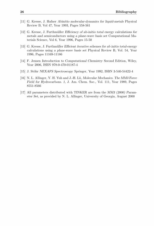
To study the orientation the values of two angles will be considered. The twoangles were studied on four different molecules. The initial simulated values werereceived assuming the (

√3×√

3)R30◦ configuration on the gold surface that canbe seen in figure A.1. This configuration will be called initial configuration fromnow on. These values together with the experimental values can be viewed at theend of this introduction.

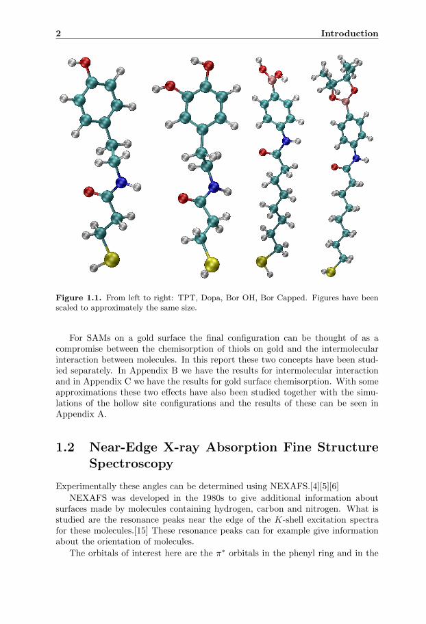
The four molecules in question will be shortened as TPT, Dopa, Bor OH, BorCapped and are displayed in figure 1.1. The angles studied are connected to theO=C-N group and the phenyl ring present in all four molecules.

1.1 Self Assembled Monolayers on a Gold Surface

Self assembled monolayers (SAMs) of thiols on Au(111) surface have been ex-tensively studied due to the fact that they arrange in densely packed stablemonolayers.[7] This together with many suggested applications for SAMs on goldsurface[7] have made these highly interesting.

The simulations that have been made for this master thesis had the purpose ofchanging the surface configuration and the molecular density. Looking at earlierwork there are some SAMs that have the same molecular density as the initialconfiguration and other SAMs have a molecular density at 60% of the initial con-figuration molecular density.[8]

For the SAMs studied here many different measurements have been made suchas X-ray Photoelectron Spectroscopy (XPS)[4][5][6] and Near-Edge X-ray Absorp-tion Fine Structure spectroscopy (NEXAFS).[4][5][6] This master thesis will onlyconsider the resulting orientation from the NEXAFS measurements.

1

2 Introduction

Figure 1.1. From left to right: TPT, Dopa, Bor OH, Bor Capped. Figures have beenscaled to approximately the same size.

For SAMs on a gold surface the final configuration can be thought of as acompromise between the chemisorption of thiols on gold and the intermolecularinteraction between molecules. In this report these two concepts have been stud-ied separately. In Appendix B we have the results for intermolecular interactionand in Appendix C we have the results for gold surface chemisorption. With someapproximations these two effects have also been studied together with the simu-lations of the hollow site configurations and the results of these can be seen inAppendix A.

1.2 Near-Edge X-ray Absorption Fine StructureSpectroscopy

Experimentally these angles can be determined using NEXAFS.[4][5][6]

NEXAFS was developed in the 1980s to give additional information aboutsurfaces made by molecules containing hydrogen, carbon and nitrogen. What isstudied are the resonance peaks near the edge of the K-shell excitation spectrafor these molecules.[15] These resonance peaks can for example give informationabout the orientation of molecules.

The orbitals of interest here are the π∗ orbitals in the phenyl ring and in the

1.2 Near-Edge X-ray Absorption Fine Structure Spectroscopy 3

peptide bond and these can be studied with NEXAFS since electrons get excitedto these orbitals close to the K-shell edge. These resonance intensities containa dependence on two unknown variables, the orientation and the X-ray incidenceangle.[15] Using symmetry arguments to eliminate one unknown variable the otherunknown variable and the orientation can be determined with two measurementsusing different X-ray incidence angles.

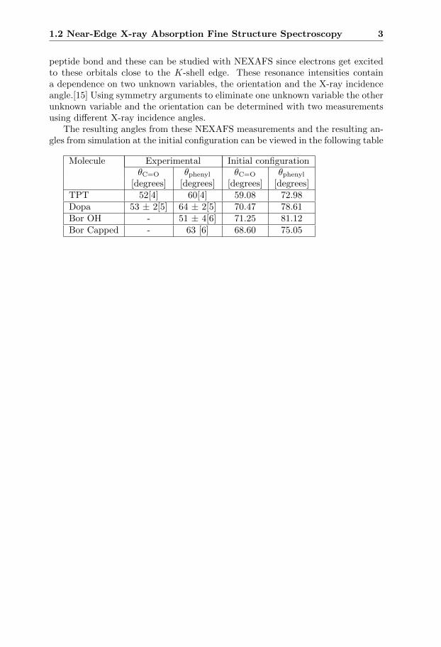
The resulting angles from these NEXAFS measurements and the resulting an-gles from simulation at the initial configuration can be viewed in the following table

Molecule Experimental Initial configurationθC=O θphenyl θC=O θphenyl

[degrees] [degrees] [degrees] [degrees]TPT 52[4] 60[4] 59.08 72.98Dopa 53 ± 2[5] 64 ± 2[5] 70.47 78.61Bor OH - 51 ± 4[6] 71.25 81.12Bor Capped - 63 [6] 68.60 75.05

4 Introduction

Chapter 2

Theory

In this chapter the theory behind some of the techniques used will be described.

2.1 Schrodinger Equation

One important problem in quantum mechanics is the problem of finding exact orapproximate solutions to the time-independent Schrodinger equation.

H |ψ〉 = E |ψ〉 (2.1)

This is considered as an eigenvalue problem where H is the Hamiltonian, |ψ〉 isthe wave function and |ψn〉 is a complete orthonormal set of eigenvectors so that

H |ψn〉 = En |ψn〉 En ≤ En+1 for all n ≥ 0 (2.2)

Equation 2.1 can only be solved exactly for simple cases that will not be consideredhere.[1]

The Hamiltonian used for N electrons and M nuclei in atomic units is

H = −N∑i=1

1

2∇2i −

M∑A=1

1

2MA∇2A−

N∑i=0

M∑A=1

ZAria

+

N∑i=1

N∑j>i

1

rij+

M∑A=1

M∑B>A

ZAZBRAB

(2.3)

The sums represent from left to right kinetic energy of electrons, kinetic energyof nuclei, Coulomb attraction energy of electrons and nuclei, Coulomb repulsionenergy between different electrons and interaction energy between different nuclei.

2.2 Hartree–Fock Theory

To simulate large systems some simplifications are needed to lower the amount ofcalculations. This is achieved by using different approximations, first of these isthe so called Born–Oppenheimer approximation that state that since the nuclei

5

6 Theory

are much heavier than the electrons the nuclei can be considered as stationary.With this 2.3 can be simplified to

H = −N∑i=1

1

2∇2i −

N∑i=0

M∑A=1

ZAria

+

N∑i=1

N∑j>i

1

rij+ Ec (2.4)

where Ec is the constant contribution to the energy by the stationary nuclei.To solve equation 2.4 multiple steps are used. Since a constant term only adds

a constant to all eigenfunctions it can be ignored and the Hamiltonian for theelectrons can be solved separately using

Helec = −N∑i=1

1

2∇2i −

N∑i=0

M∑A=1

ZAria

+

N∑i=1

N∑j>i

1

rij(2.5)

Note that the energy received from this Hamiltonian is not the total energy sincethe constant term has been neglected. Using the result of solving 2.5 and anotherassumption that the position of electrons can be approximated as stationary attheir average position the Hamiltonian for the nuclei can also be solved.[1]

Since it is known that the electron also has a spin degree of freedom this isconsidered by adding a complete and orthonormal set of two spin functions. Tochange the wave function correctly an extra constraint defined by the antisymme-try principle is added:

A many-electron wave function must be antisymmetric with respect tothe interchange of the coordinate x (both space and spin) of any twoelectrons.[1]

The antisymmetry principle is fulfilled by using so called Slater determinants.If the wavefunction is written as a determinant and each electron is placed ona separate row then changing two electrons will be the same as changing tworows and it is well known that changing two rows in a matrix will multiply thedeterminant by minus one. Because of this the antisymmetry principle will alwayshold if you use Slater determinants. It can also be realized that the antisymmetryprinciple still holds for linear combinations of Slater determinants since in the sumeach row will still only depend on one electron.

Then one more approximation is made by stating that the electron-electronCoulomb repulsion energy can be approximated by the average field generated bythe other electrons. With this the Hartree–Fock approximation has been reached.To simplify the Fock operator is introduced:

f(i) = −1

2∇2i −

M∑A=1

ZAriA

+ vHF(i) (2.6)

The Fock operator works on a single electron and vHF is the average field fromthe other electrons. To solve this, it is considered as an eigenvalue problem thatcan be solved individually for each electron. With the solutions for the electronsthe average field is updated and then the process is repeated until the solutionconverges.

2.3 Kohn–Sham Density Functional Theory 7

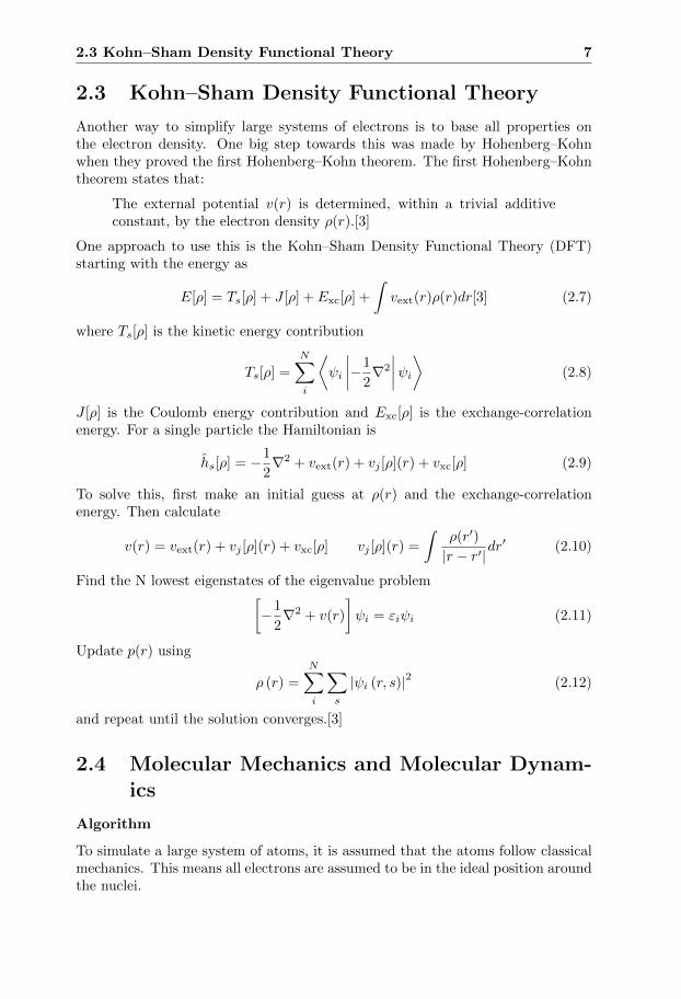
2.3 Kohn–Sham Density Functional Theory

Another way to simplify large systems of electrons is to base all properties onthe electron density. One big step towards this was made by Hohenberg–Kohnwhen they proved the first Hohenberg–Kohn theorem. The first Hohenberg–Kohntheorem states that:

The external potential v(r) is determined, within a trivial additiveconstant, by the electron density ρ(r).[3]

One approach to use this is the Kohn–Sham Density Functional Theory (DFT)starting with the energy as

E[ρ] = Ts[ρ] + J [ρ] + Exc[ρ] +

∫vext(r)ρ(r)dr[3] (2.7)

where Ts[ρ] is the kinetic energy contribution

Ts[ρ] =

N∑i

⟨ψi

∣∣∣∣−1

2∇2

∣∣∣∣ψi⟩ (2.8)

J [ρ] is the Coulomb energy contribution and Exc[ρ] is the exchange-correlationenergy. For a single particle the Hamiltonian is

hs[ρ] = −1

2∇2 + vext(r) + vj [ρ](r) + vxc[ρ] (2.9)

To solve this, first make an initial guess at ρ(r) and the exchange-correlationenergy. Then calculate

v(r) = vext(r) + vj [ρ](r) + vxc[ρ] vj [ρ](r) =

∫ρ(r′)

|r − r′|dr′ (2.10)

Find the N lowest eigenstates of the eigenvalue problem[−1

2∇2 + v(r)

]ψi = εiψi (2.11)

Update p(r) using

ρ (r) =

N∑i

∑s

|ψi (r, s)|2 (2.12)

and repeat until the solution converges.[3]

2.4 Molecular Mechanics and Molecular Dynam-ics

Algorithm

To simulate a large system of atoms, it is assumed that the atoms follow classicalmechanics. This means all electrons are assumed to be in the ideal position aroundthe nuclei.

8 Theory

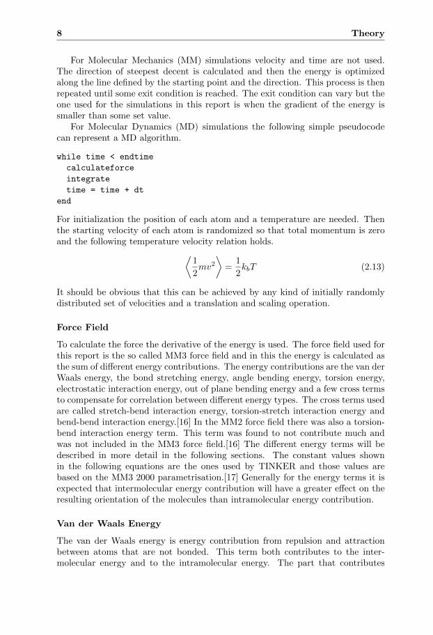
For Molecular Mechanics (MM) simulations velocity and time are not used.The direction of steepest decent is calculated and then the energy is optimizedalong the line defined by the starting point and the direction. This process is thenrepeated until some exit condition is reached. The exit condition can vary but theone used for the simulations in this report is when the gradient of the energy issmaller than some set value.

For Molecular Dynamics (MD) simulations the following simple pseudocodecan represent a MD algorithm.

while time < endtime

calculateforce

integrate

time = time + dt

end

For initialization the position of each atom and a temperature are needed. Thenthe starting velocity of each atom is randomized so that total momentum is zeroand the following temperature velocity relation holds.⟨

1

2mv2

⟩=

1

2kbT (2.13)

It should be obvious that this can be achieved by any kind of initially randomlydistributed set of velocities and a translation and scaling operation.

Force Field

To calculate the force the derivative of the energy is used. The force field used forthis report is the so called MM3 force field and in this the energy is calculated asthe sum of different energy contributions. The energy contributions are the van derWaals energy, the bond stretching energy, angle bending energy, torsion energy,electrostatic interaction energy, out of plane bending energy and a few cross termsto compensate for correlation between different energy types. The cross terms usedare called stretch-bend interaction energy, torsion-stretch interaction energy andbend-bend interaction energy.[16] In the MM2 force field there was also a torsion-bend interaction energy term. This term was found to not contribute much andwas not included in the MM3 force field.[16] The different energy terms will bedescribed in more detail in the following sections. The constant values shownin the following equations are the ones used by TINKER and those values arebased on the MM3 2000 parametrisation.[17] Generally for the energy terms it isexpected that intermolecular energy contribution will have a greater effect on theresulting orientation of the molecules than intramolecular energy contribution.

Van der Waals Energy

The van der Waals energy is energy contribution from repulsion and attractionbetween atoms that are not bonded. This term both contributes to the inter-molecular energy and to the intramolecular energy. The part that contributes

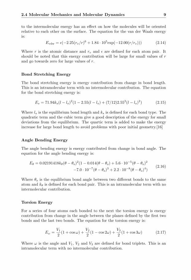
2.4 Molecular Mechanics and Molecular Dynamics 9

to the intermolecular energy has an effect on how the molecules will be orientedrelative to each other on the surface. The equation for the van der Waals energyis:

Evdw = ε(−2.25(rv/r)6 + 1.84 · 105exp(−12.00(r/rv))) (2.14)

Where r is the atomic distance and rv and ε are defined for each atom pair. Itshould be noted that this energy contribution will be large for small values of rand go towards zero for large values of r.

Bond Stretching Energy

The bond stretching energy is energy contribution from change in bond length.This is an intramolecular term with no intermolecular contribution. The equationfor the bond stretching energy is:

Es = 71.94ks(l − lo)2(1− 2.55(l − lo) + (7/12)2.552(l − lo)2) (2.15)

Where lo is the equilibrium bond length and ks is defined for each bond type. Thequadratic term and the cubic term give a good description of the energy for smalldeviations from the equilibrium. The quartic term is added to make the energyincrease for large bond length to avoid problems with poor initial geometry.[16]

Angle Bending Energy

The angle bending energy is energy contributed from change in bond angle. Theequation for the angle bending energy is:

Eθ = 0.02191418kθ(θ − θo)2(1− 0.014(θ − θo) + 5.6 · 10−5(θ − θo)2

−7.0 · 10−7(θ − θo)3 + 2.2 · 10−8(θ − θo)4)(2.16)

Where θo is the equilibrium bond angle between two different bonds to the sameatom and kθ is defined for each bond pair. This is an intramolecular term with nointermolecular contribution.

Torsion Energy

For a series of four atoms each bonded to the next the torsion energy is energycontribution from change in the angle between the planes defined by the first twobonds and the last two bonds. The equation for the torsion energy is:

Eω =V1

2(1 + cosω) +

V2

2(1− cos 2ω) +

V3

2(1 + cos 3ω) (2.17)

Where ω is the angle and V1, V2 and V3 are defined for bond triplets. This is anintramolecular term with no intermolecular contribution.

10 Theory

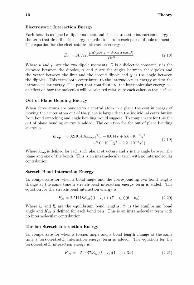
Electrostatic Interaction Energy

Each bond is assigned a dipole moment and the electrostatic interaction energy isthe term that describe the energy contributions from each pair of dipole moments.The equation for the electrostatic interaction energy is:

Eel = 14.3928µµ′(cosχ− 3 cosα cosβ)

Dr3(2.18)

Where µ and µ′ are the two dipole moments, D is a dielectric constant, r is thedistance between the dipoles, α and β are the angles between the dipoles andthe vector between the first and the second dipole and χ is the angle betweenthe dipoles. This term both contributes to the intermolecular energy and to theintramolecular energy. The part that contribute to the intermolecular energy hasan effect on how the molecules will be oriented relative to each other on the surface.

Out of Plane Bending Energy

When three atoms are bonded to a central atom in a plane the cost in energy ofmoving the center atom out of the plane is larger than the individual contributionfrom bond stretching and angle bending would suggest. To compensate for this theout of plane bending energy is added. The equation for the out of plane bendingenergy is:

Eoop = 0.02191418koopχ2(1− 0.014χ+ 5.6 · 10−5χ2

−7.0 · 10−7χ3 + 2.2 · 10−8χ4)(2.19)

Where koop is defined for each such planar structure and χ is the angle between theplane and one of the bonds. This is an intramolecular term with no intermolecularcontribution.

Stretch-Bend Interaction Energy

To compensate for when a bond angle and the corresponding two bond lengthschange at the same time a stretch-bend interaction energy term is added. Theequation for the stretch-bend interaction energy is:

Esθ = 2.51118Ksθ((l − lo) + (l′ − l′o))(θ − θo) (2.20)

Where lo and l′o are the equilibrium bond lengths, θo is the equilibrium bondangle and Ksθ is defined for each bond pair. This is an intramolecular term withno intermolecular contribution.

Torsion-Stretch Interaction Energy

To compensate for when a torsion angle and a bond length change at the sametime a torsion-stretch interaction energy term is added. The equation for thetorsion-stretch interaction energy is:

Eωs = −5.9975Kωs(l − lo)(1 + cos 3ω) (2.21)

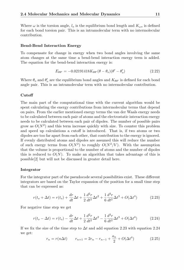
2.4 Molecular Mechanics and Molecular Dynamics 11

Where ω is the torsion angle, lo is the equilibrium bond length and Kωs is definedfor each bond torsion pair. This is an intramolecular term with no intermolecularcontribution.

Bend-Bend Interaction Energy

To compensate for change in energy when two bond angles involving the sameatom changes at the same time a bend-bend interaction energy term is added.The equation for the bend-bend interaction energy is:

Eθθ′ = −0.02191418Kθθ′(θ − θo)(θ′ − θ′o) (2.22)

Where θo and θ′o are the equilibrium bond angles and Kθθ′ is defined for each bondangle pair. This is an intramolecular term with no intermolecular contribution.

Cutoff

The main part of the computational time with the current algorithm would bespent calculating the energy contributions from intermolecular terms that dependon pairs. From the earlier mentioned energy terms the van der Waals energy needsto be calculated between each pair of atoms and the electrostatic interaction energyneeds to be calculated between each pair of dipoles. The number of possible pairsgrow as O(N2) and this term increase quickly with size. To counter this problemand speed up calculations a cutoff is introduced. That is, if two atoms or twodipoles are too far apart from each other, that contribution to the energy is ignored.If evenly distributed atoms and dipoles are assumed this will reduce the numberof such energy terms from O(N2) to roughly O(N2/V ). With the assumptionthat the volume is proportional to the number of atoms and the number of dipolesthis is reduced to O(N). To make an algorithm that takes advantage of this ispossible[2] but will not be discussed in greater detail here.

Integrator

For the integrator part of the pseudocode several possibilities exist. These differentintegrators are based on the Taylor expansion of the position for a small time stepthat can be expressed as:

r(to + ∆t) = r(to) +dr

dt∆t+

1

2

d2r

dt2∆t2 +

1

6

d3r

dt2∆t3 +O(∆t4) (2.23)

For negative time step we get

r(to −∆t) = r(to)−dr

dt∆t+

1

2

d2r

dt2∆t2 − 1

6

d3r

dt2∆t3 +O(∆t4) (2.24)

If we fix the size of the time step to ∆t and add equation 2.23 with equation 2.24we get:

rn = r(n∆t) rn+1 = 2rn − rn−1 +an2

+O(∆t4) (2.25)

12 Theory

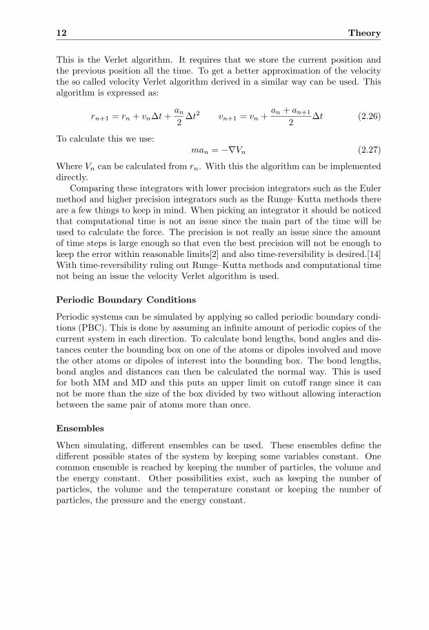
This is the Verlet algorithm. It requires that we store the current position andthe previous position all the time. To get a better approximation of the velocitythe so called velocity Verlet algorithm derived in a similar way can be used. Thisalgorithm is expressed as:

rn+1 = rn + vn∆t+an2

∆t2 vn+1 = vn +an + an+1

2∆t (2.26)

To calculate this we use:man = −∇Vn (2.27)

Where Vn can be calculated from rn. With this the algorithm can be implementeddirectly.

Comparing these integrators with lower precision integrators such as the Eulermethod and higher precision integrators such as the Runge–Kutta methods thereare a few things to keep in mind. When picking an integrator it should be noticedthat computational time is not an issue since the main part of the time will beused to calculate the force. The precision is not really an issue since the amountof time steps is large enough so that even the best precision will not be enough tokeep the error within reasonable limits[2] and also time-reversibility is desired.[14]With time-reversibility ruling out Runge–Kutta methods and computational timenot being an issue the velocity Verlet algorithm is used.

Periodic Boundary Conditions

Periodic systems can be simulated by applying so called periodic boundary condi-tions (PBC). This is done by assuming an infinite amount of periodic copies of thecurrent system in each direction. To calculate bond lengths, bond angles and dis-tances center the bounding box on one of the atoms or dipoles involved and movethe other atoms or dipoles of interest into the bounding box. The bond lengths,bond angles and distances can then be calculated the normal way. This is usedfor both MM and MD and this puts an upper limit on cutoff range since it cannot be more than the size of the box divided by two without allowing interactionbetween the same pair of atoms more than once.

Ensembles

When simulating, different ensembles can be used. These ensembles define thedifferent possible states of the system by keeping some variables constant. Onecommon ensemble is reached by keeping the number of particles, the volume andthe energy constant. Other possibilities exist, such as keeping the number ofparticles, the volume and the temperature constant or keeping the number ofparticles, the pressure and the energy constant.

Chapter 3

Methodology

In this chapter different choices and strategies which have been used to producethe results presented here will be described.

3.1 Setup of Simulations

First of all for all molecules: If the O=C-N group is considered as a dipole it makessense to alternate the direction of the dipole on different rows on the surfaceto lower the energy. This was tried in a separate simulation with the phenylring replaced with a hydrogen atom. The result from this simulation was thatalternating the dipole had an energy that was 0.79 kcal ·mol−1 per molecule lowerthan when not alternating the dipole. Since alternating the dipole had a lowerenergy, this was used in all simulations.

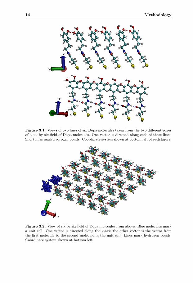
To generate a surface of molecules the following data was needed: the originalmolecule, a molecule with the direction of the dipole changed, two vector lengthsand the angle between these two vectors. The two molecules form the unit cell,the spacing between the molecules in the unit cell is determined by the secondvector and the unit cell is then copied using the two vectors until the desiredsize is reached. Along the first direction phenyl rings are organized forming π-π stacking interactions. This organization is visible in the bottom of figure 3.1.Along the other direction the phenyl are organized in a herringbone manner. Thisorganization is visible in the top of figure 3.1. The unit cell and the phenyl stackingcan be viewed in figure 3.2.

The idea was to study how the θC=O and θphenyl angles changed when theseparameters were varied. These vectors were used to generate a field of six bysix molecules with the sulfur atoms frozen and this structure was then optimized.After simulation a good correlation was found between the molecular density andboth angles and also between the molecular density and the energy as can be seenin Appendix B.

13

14 Methodology

Figure 3.1. Views of two lines of six Dopa molecules taken from the two different edgesof a six by six field of Dopa molecules. One vector is directed along each of these lines.Short lines mark hydrogen bonds. Coordinate system shown at bottom left of each figure.

Figure 3.2. View of six by six field of Dopa molecules from above. Blue molecules marka unit cell. One vector is directed along the x-axis the other vector is the vector fromthe first molecule to the second molecule in the unit cell. Lines mark hydrogen bonds.Coordinate system shown at bottom left.

3.2 Filters for Simulations 15

3.2 Filters for Simulations

Several of the simulations resulted in structures with no physical meaning. Todeal with these different filters were designed. First of all one structure typeconsisting of local clusters of molecules or molecules being directed in seeminglyrandom directions. These simulations could be filtered out by measuring somespecific atom position and see how close it was to the gridlike starting structure.Although this could seem rather risky it could be noticed that most simulationsthat ended ordered had the gridlike structure to a very high precision.

One class of unwanted simulation results were produced by folding of molecules.Since this was usually not present on all molecules these were detected by a highdifference between the maximum z-coordinate and minimum z-coordinate of someatom positioned in the top group.

The final filter used was starting with a position optimized closer to the sim-ulated position. These optimized positions were obtained using visual inspectionof the resulting configurations at densities closer to the position that would besimulated. This eliminated the need for other filters since the resulting configura-tions did not have the two problems described above if they started at a positionclose enough to the one in the optimized simulation. All plotted points have beenproduced only by using a good starting position.

3.3 VASP Simulations

For the VASP simulations five three by three layers of gold were used. The start-ing configuration of methanethiol was obtained in a separate simulation and theentire methanethiol was translated between different VASP simulations. For eachsimulation the sulfur atom was frozen in x and y direction and the bottom twogold layers were completely frozen.

Periodic cubic splines were used together with the results from these simula-tions to get a good approximation of the potential energy surface. The resultingcurve together with the simulated data can be seen in Appendix C.

3.4 Setup of Hollow Site Simulations

One set of simulations were made to determine what configuration has the closestmatch to the experimental angle and also has a favorable placement on the goldsurface.

To determine what configurations to test the potential energy surface shown infigure C.1 was used. In this figure it can be seen that the first hollow site positionhas lowest energy. However there is another hollow site position that has similarenergy. To be able to define all hollow sites with two vectors and one angle asbefore, the position of the sulfur atoms was allowed to be translated from the idealposition.

The energy required to use these translated positions instead of the ideal oneswas calculated to 1.6 kcal · mol−1 per molecule using the periodic cubic spline

16 Methodology

approximation shown in figure C.1.From the set of points made by all such translated hollow sites all pairs of two

vectors were constructed and from these all pairs of vectors that would lead to adensity in an acceptable range were picked. The configuration for all these pairsof vectors were generated and optimized and from these the closest match to theexperimental angles is shown in Appendix A.

Chapter 4

Computational Details

DFT calculations were performed with the Vienna Ab-initio Simulation Pack-age (VASP)[11][12][13] using projector augmented-wave (PAW) potential,[9][10]default energy cutoff and energy difference cutoff of 10−4 were used. Other calcu-lations were performed with TINKER minimize using the MM3 force field, a cutoffof 10 A was used and simulations were stopped when the gradient was less than10−4. All calculations were performed on the Kappa supercomputer at Linkopinguniversity.

For the TINKER simulations the required θC=O and θphenyl angles were ex-tracted from the resulting configurations with vector algebra. For the phenyl ringevery second carbon atom was used to make a plane, from this plane the normalvector was calculated and then finally the angle between the normal of the planeand the z-axis was calculated. For the O=C-N group all three atoms were used tomake a plane and the same procedure as above was applied to get the angle.

17

18 Computational Details

Chapter 5

Results and Discussion

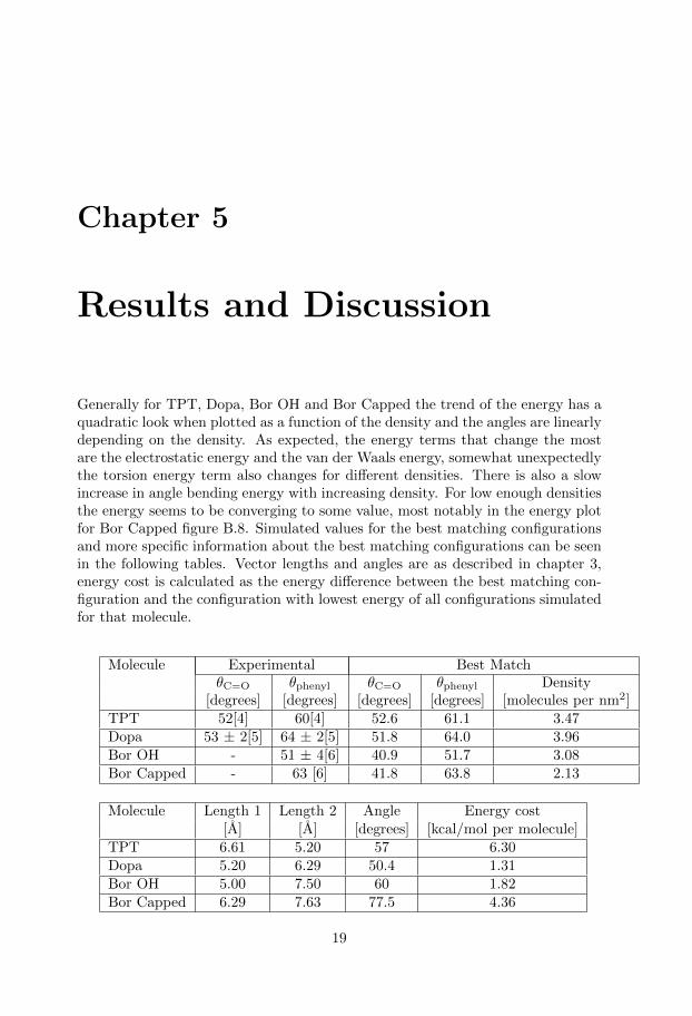
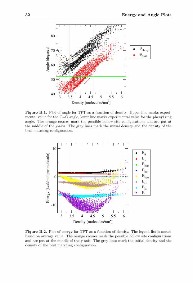
Generally for TPT, Dopa, Bor OH and Bor Capped the trend of the energy has aquadratic look when plotted as a function of the density and the angles are linearlydepending on the density. As expected, the energy terms that change the mostare the electrostatic energy and the van der Waals energy, somewhat unexpectedlythe torsion energy term also changes for different densities. There is also a slowincrease in angle bending energy with increasing density. For low enough densitiesthe energy seems to be converging to some value, most notably in the energy plotfor Bor Capped figure B.8. Simulated values for the best matching configurationsand more specific information about the best matching configurations can be seenin the following tables. Vector lengths and angles are as described in chapter 3,energy cost is calculated as the energy difference between the best matching con-figuration and the configuration with lowest energy of all configurations simulatedfor that molecule.

Molecule Experimental Best MatchθC=O θphenyl θC=O θphenyl Density

[degrees] [degrees] [degrees] [degrees] [molecules per nm2]TPT 52[4] 60[4] 52.6 61.1 3.47Dopa 53 ± 2[5] 64 ± 2[5] 51.8 64.0 3.96Bor OH - 51 ± 4[6] 40.9 51.7 3.08Bor Capped - 63 [6] 41.8 63.8 2.13

Molecule Length 1 Length 2 Angle Energy cost[A] [A] [degrees] [kcal/mol per molecule]

TPT 6.61 5.20 57 6.30Dopa 5.20 6.29 50.4 1.31Bor OH 5.00 7.50 60 1.82Bor Capped 6.29 7.63 77.5 4.36

19

20 Results and Discussion

5.1 Methanethiolate on Au

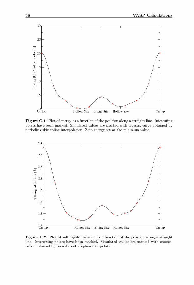
In the energy plot for methanethiolate on a gold surface figure C.1 local minimaat both hollow sites and a global minimum at the first one are visible. The energyrequired to pass the bridge site is quite high which could indicate that if this isthe same for a simulation with other molecules then the molecules can not beconsidered to move freely on the gold surface and a good starting configurationwould be needed to reach optimum.

In the sulfur-gold distance plot figure C.2 the distance varies almost in thesame way as the energy in figure C.1.

It was noted from visual inspection of the simulations that the change in struc-ture was very low. This means that a more extensive study would be needed tofind the correct structure.

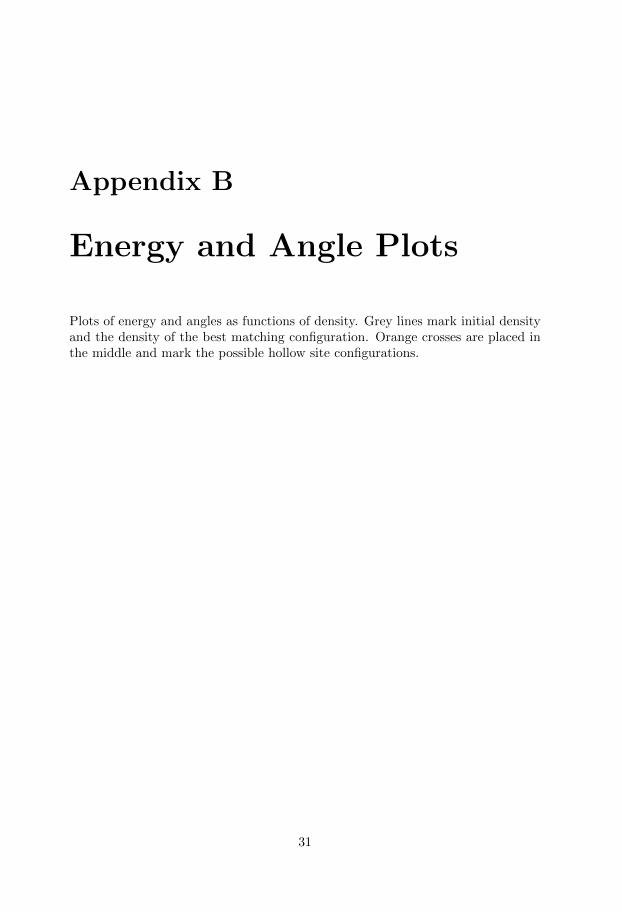
5.2 TPT

In the energy plot of TPT figure B.2 the energy has a quadratic trend with aminimum at slightly lower density than the initial configuration. In the angleplot for TPT figure B.1 there is a linear dependence between the density and theangles.

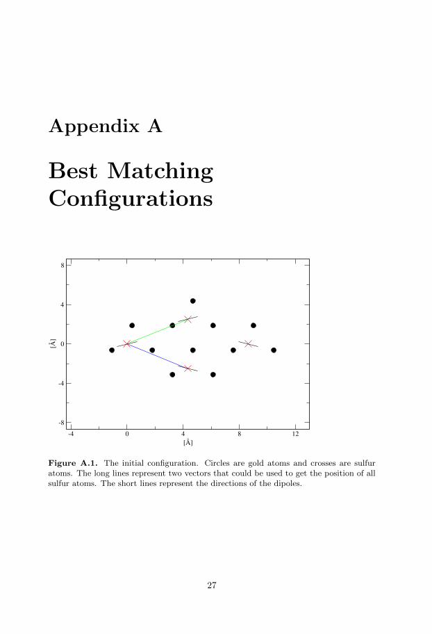
The configuration with best matching angles for TPT among the hollow sitesimulations is visible in figure A.2 and has a much lower density than the minimumin the energy plot. In the angle plot the two angle curves match the experimentalvalues only at the edge of the curve and between two possible hollow site configu-rations.

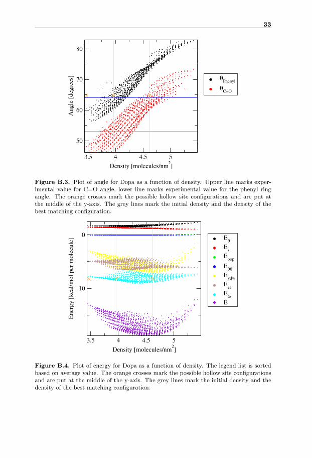
5.3 Dopa

In the energy plot of Dopa figure B.4 the energy has a quadratic trend with aminimum at slightly lower density than the initial configuration. In the angleplot for Dopa figure B.3 there is a linear dependence between the density and theangles.

The configuration with best matching angles for Dopa among the hollow sitesimulations is visible in figure A.3 and has a lower density than the minimum inthe energy plot. In the angle plot both angle curves pass the experimental valueat the density for one hollow site configuration and this density is the same as thebest matching configuration.

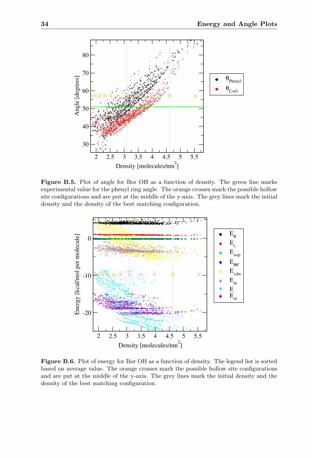
5.4 Bor OH

In the energy plot of Bor OH figure B.6 the energy has a quadratic trend with aminimum close to the initial configuration. In the angle plot for Bor OH figureB.5 there is a linear dependence between the density and the angles.

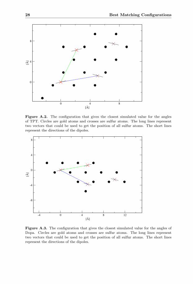
The configuration with best matching angle for Bor OH among the hollow sitesimulations is visible in figure A.4 and has a much lower density than the minimum

5.5 Bor Capped 21

in the energy plot. The large difference in energy from simulations close to eachother in density suggests that new simulations with better initial state are neededto get a clearer view of the energy dependence.

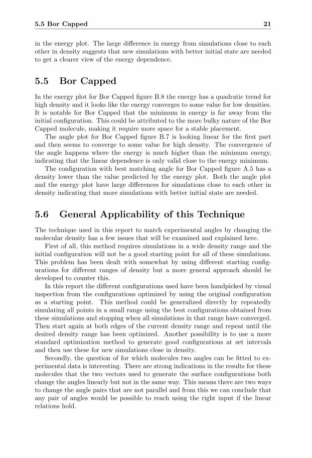
5.5 Bor Capped

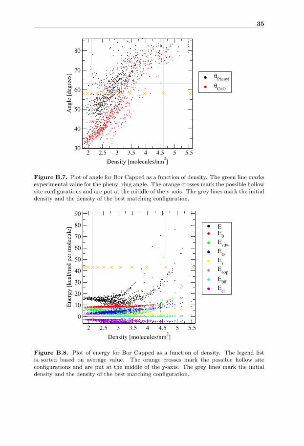
In the energy plot for Bor Capped figure B.8 the energy has a quadratic trend forhigh density and it looks like the energy converges to some value for low densities.It is notable for Bor Capped that the minimum in energy is far away from theinitial configuration. This could be attributed to the more bulky nature of the BorCapped molecule, making it require more space for a stable placement.

The angle plot for Bor Capped figure B.7 is looking linear for the first partand then seems to converge to some value for high density. The convergence ofthe angle happens where the energy is much higher than the minimum energy,indicating that the linear dependence is only valid close to the energy minimum.

The configuration with best matching angle for Bor Capped figure A.5 has adensity lower than the value predicted by the energy plot. Both the angle plotand the energy plot have large differences for simulations close to each other indensity indicating that more simulations with better initial state are needed.

5.6 General Applicability of this Technique

The technique used in this report to match experimental angles by changing themolecular density has a few issues that will be examined and explained here.

First of all, this method requires simulations in a wide density range and theinitial configuration will not be a good starting point for all of these simulations.This problem has been dealt with somewhat by using different starting config-urations for different ranges of density but a more general approach should bedeveloped to counter this.

In this report the different configurations used have been handpicked by visualinspection from the configurations optimized by using the original configurationas a starting point. This method could be generalized directly by repeatedlysimulating all points in a small range using the best configurations obtained fromthese simulations and stopping when all simulations in that range have converged.Then start again at both edges of the current density range and repeat until thedesired density range has been optimized. Another possibility is to use a morestandard optimization method to generate good configurations at set intervalsand then use these for new simulations close in density.

Secondly, the question of for which molecules two angles can be fitted to ex-perimental data is interesting. There are strong indications in the results for thesemolecules that the two vectors used to generate the surface configurations bothchange the angles linearly but not in the same way. This means there are two waysto change the angle pairs that are not parallel and from this we can conclude thatany pair of angles would be possible to reach using the right input if the linearrelations hold.

22 Results and Discussion

The hollow site configuration criteria put a much stronger restriction on thedensity than it puts on the vector pair used. This means that this criteria is notas restricting as it would appear to be.

Third, for a given configuration multiple different unit cells can be used togenerate it. From visual inspection it was noticed that many simulations getstuck halfway through trying to align every molecule to a configuration that couldhave been generated by using a different unit cell. Clearly only one unit cell fora given configuration can be optimal. To speed up calculations and avoid thisproblem, a way to determine the optimal unit cell for a given configuration shouldbe investigated.

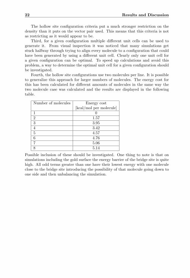
Fourth, the hollow site configurations use two molecules per line. It is possibleto generalize this approach for larger numbers of molecules. The energy cost forthis has been calculated for different amounts of molecules in the same way thetwo molecule case was calculated and the results are displayed in the followingtable.

Number of molecules Energy cost[kcal/mol per molecule]

1 02 1.573 3.954 3.425 4.576 4.767 5.068 5.14

Possible inclusion of these should be investigated. One thing to note is that onsimulations including the gold surface the energy barrier of the bridge site is quitehigh. All odd terms greater than one have their lowest energy with one moleculeclose to the bridge site introducing the possibility of that molecule going down toone side and then unbalancing the simulation.

Chapter 6

Conclusions & Perspectives

A theoretical analysis of the orientation and energy of TPT, Dopa, Bor OH andBor Capped for different surface configurations has been made to find a possibleexplanation of the difference in experimental and theoretical orientation, specifi-cally the value of two angles.

The results show that the minimum in energy has a lower density for TPT,Dopa and Bor OH compared to the initial configuration. For Bor Capped theminimum in energy is at a significantly lower density than the initial configuration.

Matching the angles with experimental values can be done by lowering thedensity using hollow site configurations on a gold surface. The resulting den-sity ordered highest to lowest is: Initial configuration, Dopa, TPT, Bor OH, BorCapped.

An analysis of methanethiolate on a gold surface has also been made to preparefor a future inclusion of the gold surface in the simulation and it indicates that weneed a good starting configuration since the energy barrier to pass the bridge siteis quite large.

Future studies should focus on strategies for finding better starting configura-tions, methods to include the gold surface in the simulation, methods to includethe temperature in the simulation and more comparisons with experimental data.

23

24 Conclusions & Perspectives

Bibliography

[1] Attila Szabo and Niel S. Ostlund. Modern Quantum Chemistry: Introductionto Advanced Electronic Structure Theory. Dover Edition, Dover Publications,Inc, Year 1996, ISBN 0-486-69186-1

[2] Daan Frenkel and Berend Smit. Understanding Molecular Simulation: FromAlgorithms to Applications. Second Edition, Academic Press, Year 2001,ISBN 0-12-267351-4

[3] Robert G. Parr and Weitao Yang Density-Functional Theory of Atoms andMolecules Oxford University Press, Year 1994, ISBN 0-19-509276-7

[4] Rodrigo M. Petoral Jr. and Kajsa Uvdal XPS and NEXAFS study of tyrosine-terminated propanethiol assembled on gold Journal of Electron Spectroscopyand Related Phenomena, Vol. 128, Year 2003, Pages 159-164

[5] Rodrigo M. Petoral Jr. and Kajsa Uvdal Structural Investigation of 3,4-Dihydroxyphenylalanine-Terminated Propanethiol Assembled on Gold J.Phys. Chem. B, Vol. 107, Year 2003, Pages 13396-13402

[6] Cecilia Vahlberg, Mathieu Linares, Patrick Norman and Kajsa Uvdal Phenyl-boronic Ester- and Phenylboronic Acid-Terminated Alkanethiols on Gold Sur-faces Journal of Physical Chemistry, Vol. 116, Year 2012, Pages 796-806

[7] Borys Szefczyk, Ricardo Franco, Jose A.N.F. Gnomes, M Natalia D.S.Cordeiro Structure of the interface between water and self-assembled monolay-ers of neutral, anionic and cationic alkane thiols Journal of Molecular Struc-ture: THEOCHEM, Vol. 946, Year 2010, Pages 83-87

[8] Yu-Tai Tao, Chien-Ching Wu, Ji-Yang Eu, Wen-Ling Lin Structure Evolutionof Aromatic-Derivatized Thiol Monolayers on Evaporated Gold LANGMUIR,Vol. 13, Year 1997, Pages 4018-4023

[9] G. Kresse, D. Joubert From ultrasoft pseudopotentials to the projectoraugmented-wave method Physical Review B, Vol 59, Year 1999, Pages 1758-1775

[10] G. Kresse, J. Hafner Norm-conserving and ultrasoft pseudopotentials for first-row and transition-elements Journal of Physics: Condensed Matter, Vol 6,Year 1994, Pages 8245-8257

25

26 Bibliography

[11] G. Kresse, J. Hafner Abinitio molecular-dynamics for liquid-metals PhysicalReview B, Vol 47, Year 1993, Pages 558-561

[12] G. Kresse, J. Furthmuller Efficiency of ab-initio total energy calculations formetals and semiconductors using a plane-wave basis set Computational Ma-terials Science, Vol 6, Year 1996, Pages 15-50

[13] G. Kresse, J. Furthmuller Efficient iterative schemes for ab initio total-energycalculations using a plane-wave basis set Physical Review B, Vol. 54, Year1996, Pages 11169-11186

[14] F. Jensen Introduction to Computational Chemistry Second Edition, Wiley,Year 2006, ISBN 978-0-470-01187-4

[15] J. Stohr NEXAFS Spectroscopy Springer, Year 1992, ISBN 3-540-54422-4

[16] N. L. Allinger, Y. H. Yuh and J.-H. Lii, Molecular Mechanics. The MM3 ForceField for Hydrocarbons. 1, J. Am. Chem. Soc., Vol. 111, Year 1989, Pages8551-8566

[17] All parameters distributed with TINKER are from the MM3 (2000) Param-eter Set, as provided by N. L. Allinger, University of Georgia, August 2000

Appendix A

Best MatchingConfigurations

-4 0 4 8 12[Å]

-8

-4

0

4

8

[Å]

Figure A.1. The initial configuration. Circles are gold atoms and crosses are sulfuratoms. The long lines represent two vectors that could be used to get the position of allsulfur atoms. The short lines represent the directions of the dipoles.

27

28 Best Matching Configurations

0 4 8[Å]

0

4

8

[Å]

Figure A.2. The configuration that gives the closest simulated value for the anglesof TPT. Circles are gold atoms and crosses are sulfur atoms. The long lines representtwo vectors that could be used to get the position of all sulfur atoms. The short linesrepresent the directions of the dipoles.

-4 0 4 8 12[Å]

-8

-4

0

4

8

[Å]

Figure A.3. The configuration that gives the closest simulated value for the angles ofDopa. Circles are gold atoms and crosses are sulfur atoms. The long lines representtwo vectors that could be used to get the position of all sulfur atoms. The short linesrepresent the directions of the dipoles.

29

-4 0 4 8[Å]

-4

0

4

8

12

[Å]

Figure A.4. The configuration that gives the closest simulated value for the angle ofBor OH. Circles are gold atoms and crosses are sulfur atoms. The long lines representtwo vectors that could be used to get the position of all sulfur atoms. The short linesrepresent the directions of the dipoles.

-4 0 4 8[Å]

-4

0

4

8

12

[Å]

Figure A.5. The configuration that gives the closest simulated value for the angle of BorCapped. Circles are gold atoms and crosses are sulfur atoms. The long lines representtwo vectors that could be used to get the position of all sulfur atoms. The short linesrepresent the directions of the dipoles.

30 Best Matching Configurations

Appendix B

Energy and Angle Plots

Plots of energy and angles as functions of density. Grey lines mark initial densityand the density of the best matching configuration. Orange crosses are placed inthe middle and mark the possible hollow site configurations.

31

32 Energy and Angle Plots

3 3.5 4 4.5 5 5.5 6

Density [molecules/nm2]

40

50

60

70

80

An

gle

[d

egre

es]

θPhenyl

θC=O

Figure B.1. Plot of angle for TPT as a function of density. Upper line marks experi-mental value for the C=O angle, lower line marks experimental value for the phenyl ringangle. The orange crosses mark the possible hollow site configurations and are put atthe middle of the y-axis. The grey lines mark the initial density and the density of thebest matching configuration.

3 3.5 4 4.5 5 5.5 6

Density [molecules/nm2]

-10

0

10

Ener

gy [

kca

l/m

ol

per

mole

cule

] Eθ

Es

Eoop

Eθθ’

Evdw

Eel

Eω

E

Figure B.2. Plot of energy for TPT as a function of density. The legend list is sortedbased on average value. The orange crosses mark the possible hollow site configurationsand are put at the middle of the y-axis. The grey lines mark the initial density and thedensity of the best matching configuration.

33

3.5 4 4.5 5

Density [molecules/nm2]

50

60

70

80

An

gle

[d

egre

es]

θPhenyl

θC=O

Figure B.3. Plot of angle for Dopa as a function of density. Upper line marks exper-imental value for C=O angle, lower line marks experimental value for the phenyl ringangle. The orange crosses mark the possible hollow site configurations and are put atthe middle of the y-axis. The grey lines mark the initial density and the density of thebest matching configuration.

3.5 4 4.5 5

Density [molecules/nm2]

-10

0

Ener

gy [

kca

l/m

ol

per

mole

cule

] Eθ

Es

Eoop

Eθθ’

Evdw

Eel

Eω

E

Figure B.4. Plot of energy for Dopa as a function of density. The legend list is sortedbased on average value. The orange crosses mark the possible hollow site configurationsand are put at the middle of the y-axis. The grey lines mark the initial density and thedensity of the best matching configuration.

34 Energy and Angle Plots

2 2.5 3 3.5 4 4.5 5 5.5

Density [molecules/nm2]

30

40

50

60

70

80

An

gle

[d

egre

es]

θPhenyl

θC=O

Figure B.5. Plot of angle for Bor OH as a function of density. The green line marksexperimental value for the phenyl ring angle. The orange crosses mark the possible hollowsite configurations and are put at the middle of the y-axis. The grey lines mark the initialdensity and the density of the best matching configuration.

2 2.5 3 3.5 4 4.5 5 5.5

Density [molecules/nm2]

-20

-10

0

Ener

gy [

kca

l/m

ol

per

mole

cule

] Eθ

Es

Eoop

Eθθ’

Evdw

Eω

EE

el

Figure B.6. Plot of energy for Bor OH as a function of density. The legend list is sortedbased on average value. The orange crosses mark the possible hollow site configurationsand are put at the middle of the y-axis. The grey lines mark the initial density and thedensity of the best matching configuration.

35

2 2.5 3 3.5 4 4.5 5 5.5

Density [molecules/nm2]

30

40

50

60

70

80

An

gle

[d

egre

es]

θPhenyl

θC=O

Figure B.7. Plot of angle for Bor Capped as a function of density. The green line marksexperimental value for the phenyl ring angle. The orange crosses mark the possible hollowsite configurations and are put at the middle of the y-axis. The grey lines mark the initialdensity and the density of the best matching configuration.

2 2.5 3 3.5 4 4.5 5 5.5

Density [molecules/nm2]

0

10

20

30

40

50

60

70

80

90

Ener

gy [

kca

l/m

ol

per

mole

cule

] EE

θ

Evdw

Eω

Es

Eoop

Eθθ’

Eel

Figure B.8. Plot of energy for Bor Capped as a function of density. The legend listis sorted based on average value. The orange crosses mark the possible hollow siteconfigurations and are put at the middle of the y-axis. The grey lines mark the initialdensity and the density of the best matching configuration.

36 Energy and Angle Plots

Appendix C

VASP Calculations

For both figures in this appendix: Simulated values are marked with crosses andthe marked curve is obtained from periodic cubic spline interpolation. Simulatedvalues were obtained using VASP to optimize a methanethiol molecule on a goldsurface. For the methanethiol the hydrogen connected to the sulfur had beenremoved.

37

38 VASP Calculations

On top Hollow Site Bridge Site Hollow Site On top0

5

10

15

20

25

30

Ener

gy [

kca

l/m

ol

per

mole

cule

]

Figure C.1. Plot of energy as a function of the position along a straight line. Interestingpoints have been marked. Simulated values are marked with crosses, curve obtained byperiodic cubic spline interpolation. Zero energy set at the minimum value.

On top Hollow Site Bridge Site Hollow Site On top1.7

1.8

1.9

2

2.1

2.2

2.3

2.4

Sulf

ur-g

old

dist

ance

[Å

]

Figure C.2. Plot of sulfur-gold distance as a function of the position along a straightline. Interesting points have been marked. Simulated values are marked with crosses,curve obtained by periodic cubic spline interpolation.