MA STER’S THESIS

Optimisation of fresh water consumptionfor Doggy AB using simulation

Maja Olsson UppenbergMoa Ryberg

Department of Mathematics

CHALMERS UNIVERSITY OF TECHNOLOGYGÖTEBORG UNIVERSITYGöteborg Sweden 2005

Thesis for the Degree of Master of Science

Optimisation of fresh water

consumption for Doggy AB using

simulation

Maja Olsson UppenbergMoa Ryberg

Department of MathematicsChalmers University of Technology and Göteborg University

SE-412 96 Göteborg, SwedenGöteborg, December 2005

Matematiskt centrumGöteborg 2005

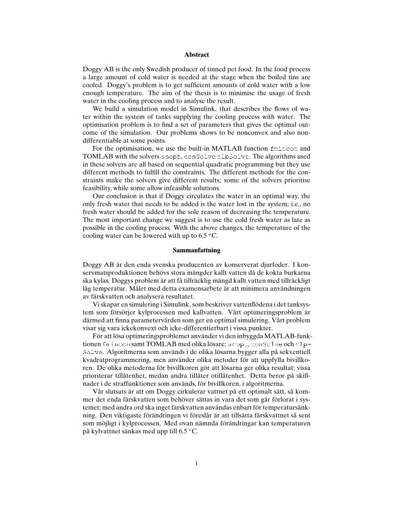
Abstract

Doggy AB is the only Swedish producer of tinned pet food. In the food processa large amount of cold water is needed at the stage when the boiled tins arecooled. Doggy’s problem is to get sufficient amounts of cold water with a lowenough temperature. The aim of the thesis is to minimise the usage of freshwater in the cooling process and to analyse the result.

We build a simulation model in Simulink, that describes the flows of wa-ter within the system of tanks supplying the cooling process with water. Theoptimisation problem is to find a set of parameters that gives the optimal out-come of the simulation. Our problems shows to be nonconvex and also non-differentiable at some points.

For the optimisation, we use the built-in MATLAB function fmin on andTOMLAB with the solvers snopt, onSolve nlpSolve. The algorithms usedin these solvers are all based on sequential quadratic programming but they usedifferent methods to fulfill the constraints. The different methods for the con-straints make the solvers give different results; some of the solvers prioritisefeasibility, while some allow infeasible solutions.

Our conclusion is that if Doggy circulates the water in an optimal way, theonly fresh water that needs to be added is the water lost in the system; i.e., nofresh water should be added for the sole reason of decreasing the temperature.The most important change we suggest is to use the cold fresh water as late aspossible in the cooling process. With the above changes, the temperature of thecooling water can be lowered with up to 6.5 ÆC.

Sammanfattning

Doggy AB är den enda svenska producenten av konserverat djurfoder. I kon-servmatsproduktionen behövs stora mängder kallt vatten då de kokta burkarnaska kylas. Doggys problem är att få tillräcklig mängd kallt vatten med tillräckligtlåg temperatur. Målet med detta examensarbete är att minimera användningenav färskvatten och analysera resultatet.

Vi skapar en simulering i Simulink, som beskriver vattenflödena i det tanksys-tem som försörjer kylprocessen med kallvatten. Vårt optimeringsproblem ärdärmed att finna parametervärden som ger en optimal simulering. Vårt problemvisar sig vara ickekonvext och icke-differentierbart i vissa punkter.

För att lösa optimeringsproblemet använder vi den inbyggda MATLAB-funk-tionen fmin on samt TOMLAB med olika lösare: snopt, onSolve och nlp-Solve. Algoritmerna som används i de olika lösarna bygger alla på sekventiellkvadratprogrammering, men använder olika metoder för att uppfylla bivillko-ren. De olika metoderna för bivillkoren gör att lösarna ger olika resultat; vissaprioriterar tillåtenhet, medan andra tillåter otillåtenhet. Detta beror på skill-nader i de straffunktioner som används, för bivillkoren, i algoritmerna.

Vår slutsats är att om Doggy cirkulerar vattnet på ett optimalt sätt, så kom-mer det enda färskvatten som behöver sättas in vara det som går förlorat i sys-temet; med andra ord ska inget färskvatten användas enbart för temperatursänk-ning. Den viktigaste förändringen vi föreslår är att tillsätta färskvattnet så sentsom möjligt i kylprocessen. Med ovan nämnda förändringar kan temperaturenpå kylvattnet sänkas med upp till 6.5 ÆC.

i

Acknowledgments

We would like to thank our supervisor Professor Michael Patriksson at the De-partment of Mathematical Sciences at Chalmers University of Technology andGöteborg University. You are always honest and cheer us up when we need itthe most. You give us space to develop our own ideas and to use our knowledge,and, of course, thank you for the great pictures of the factory.

We would also like to thank Doggy AB, especially Torbjörn Pettersson, GöranLundevall and Lars-Åke Larsson. You give us the information we need and havepatience with us when our calculations seem to take forever.

We would also like to thank Anna Nyström for the cooperation with Simulink.Without your help to get started, we would probably still be working with thesimulations.

We would also like to thank Inga Lasson at Alfa Laval for taking time to helpus with heat exchanger calculations.

Finally we would like to thank John and Tony for being there for us whenwe need it the most. Thank you for taking care of us after long working days.Behind every successful woman, there is a supporting husband.

ii

Contents

1 Introduction 1

1.1 About Doggy AB . . . . . . . . . . . . . . . . . . . . . . . . . . . 11.2 The aim of the project . . . . . . . . . . . . . . . . . . . . . . . . . 11.3 Methods . . . . . . . . . . . . . . . . . . . . . . . . . . . . . . . . 21.4 Outline . . . . . . . . . . . . . . . . . . . . . . . . . . . . . . . . . 2

2 The production 22.1 Tank 1 . . . . . . . . . . . . . . . . . . . . . . . . . . . . . . . . . . 52.2 Tank 2 . . . . . . . . . . . . . . . . . . . . . . . . . . . . . . . . . . 62.3 Tank 3 . . . . . . . . . . . . . . . . . . . . . . . . . . . . . . . . . . 72.4 Tank 4 . . . . . . . . . . . . . . . . . . . . . . . . . . . . . . . . . . 72.5 Tank C . . . . . . . . . . . . . . . . . . . . . . . . . . . . . . . . . 8

2.5.1 Dilution . . . . . . . . . . . . . . . . . . . . . . . . . . . . 92.5.2 Night cooling . . . . . . . . . . . . . . . . . . . . . . . . . 92.5.3 Batch . . . . . . . . . . . . . . . . . . . . . . . . . . . . . . 9

3 The mathematical model 9

3.1 General expressions . . . . . . . . . . . . . . . . . . . . . . . . . . 93.2 Equations describing the system of tanks . . . . . . . . . . . . . . 103.3 Additional constraints . . . . . . . . . . . . . . . . . . . . . . . . 133.4 A summary of the problem . . . . . . . . . . . . . . . . . . . . . . 15

4 The simulation in Simulink 16

5 The optimisation 18

5.1 Description of the problem . . . . . . . . . . . . . . . . . . . . . . 185.2 The solvers EGO, rbfSolve and fminsearch . . . . . . . . . . . . . 225.3 SQP . . . . . . . . . . . . . . . . . . . . . . . . . . . . . . . . . . . 225.4 The built-in MATLAB function fmincon . . . . . . . . . . . . . . 235.5 The TOMLAB solver snopt . . . . . . . . . . . . . . . . . . . . . 245.6 The TOMLAB solver conSolve . . . . . . . . . . . . . . . . . . . 245.7 The TOMLAB solver nlpSolve . . . . . . . . . . . . . . . . . . . 24

6 Results 25

6.1 Optimisation . . . . . . . . . . . . . . . . . . . . . . . . . . . . . . 266.2 Improvements . . . . . . . . . . . . . . . . . . . . . . . . . . . . . 33

7 Discussion 36

8 Further possible developments 37

References 38

A Heat balance I

B Overflow II

C Constants III

iii

D Term descriptions IV

iv

1 Introduction

1.1 About Doggy AB

Doggy AB is one of the main producers of pet food in Sweden. The factory islocated in Vårgårda, 70 km north east of Gothenburg, and produces both pel-lets and tinned food. Doggy’s factory makes about 70 % of the pellets and 100% of the tinned pet food produced in Sweden. The primary market is Sweden,but Doggy also exports, mainly to England and Germany.[Pet05] In the tin pro-

duction, one production cost stems from the input of extra water in the coolingof the boiled food. The aim of the project, which is made on behalf of Doggy,is to minimise the total amount of added water and to find its optimal use. Thefactory is divided into two sub factories: one for the pellets food and one for thetinned food. This thesis will only consider the tin production so from now on, wewill focus on this part of the factory, which is split into two parts, one for the pro-duction of the original aluminium tins and one for a recently started Tetra Pakproduction line. The food is boiled in the tins (both the aluminium and TetraPak) and thereafter cooled for handling reasons. The cooling of the tins has tofinish within 35 minutes, due to hygiene restrictions and time constraints. Toachieve a sufficient cooling, large quantities of cold water are needed. The cool-ing water can be reused by going through a heat exchanger and a series of tanks.During the summer when the temperature in the system is generally higher, it isdifficult to lower the temperature of the food sufficiently and efficiently. A sim-ple but expensive solution to decrease the temperature of the cooling water is toadd cold fresh water. Some fresh water must be inserted, since there is a loss ofwater in the production, but apart from that, excessive water will just be lost to anearby narrow river. An optimisation of the circulation of the cooling water willbring down the usage of fresh water, which is the objective of this thesis.

The circulation of the water can be controlled by changing the parameters inthe regulations of the system. The problem has several constraints: the coolingof the tins has to finish within 35 minutes (which can be achieved only if thetemperature of the cooling water is below 20 ÆC), the tanks are not allowed torun empty and there are pumps and pipes in the systems with limited capacities.

1.2 The aim of the project

The goal of this thesis is to minimise the waste of fresh water and to keep thecooling water at a low temperature, by finding an optimal circulation of the wa-ter in the tin production. Flows going into and out from the system can be rear-ranged as long as necessary constraints are fulfilled.

We will not consider very drastic solutions, for example significant rebuild-ings of the factory. Even very expensive solutions are ignored; even though some

1

kind of electrical cooling system would work, the cost of it would vastly exceedthe money saved from the decreased water usage.

1.3 Methods

In this project, a broad range of tasks has been necessary to perform: frommeasurements to advanced calculations. The first thing we did was getting anoverview over the system by mapping it out. This part of the project was merelydone at the factory where we measured flows, looked at blueprints over the tanksystem, and registered temperatures. We measured the flows with a flow mea-surement tool during a day with normal production.

The next part of the project is to model the system mathematically. The equa-tions describing the problem are non-linear and time dependent and set up as asystem of ordinary differential equations (ODEs). This system is very complexand it is too difficult, if not impossible, to solve it explicitly. Therefore, we per-form a simulation of the problem to be used as a "black-box" in the optimisation.Our task is then to find the ingoing parameters to the simulation that result inthe optimal circulation of the water. We get an optimisation problem where theconstants and some variables are set by us, and other variables are obtained fromthe simulation. The modelling and simulation of the problem is made with theMATLAB toolbox Simulink and to solve the optimisation problem, MATLAB isused with different solvers. We have chosen to use the built-in MATLAB func-tion fmin on, and also use three of TOMLAB’s solvers: snopt, onSolveand nlpSolve.

1.4 Outline

In the next section a more detailed description of the production is presented,especially of the tanks and the cooling process. The equations describing thesystem are presented in Section 3, where we also discuss the properties of theproblem. A description of the Simulink simulation is shown in Section 4. In Sec-tion 5 the optimisation problem is discussed and analysed and some solvers arepresented. The differences between the solvers are also discussed. In Sections 6and 7 the results of the optimisation are shown and discussed. Finally, in Section8 further developments of the system are suggested. In Appendix A and B somederivations of mathematical expressions are shown; the constants used are foundin Appendix C and in Appendix D some term descriptions are explained.

2 The production

Cat and dog food is made out of different kinds of meat and additives, for ex-ample vitamins. The ingredients are mixed and poured into tins before the boil-ing procedure takes place in an autoclave.[Pet05] An autoclave is a closed sys-tem where physical reactions take place with a high temperature and under highpressure.[NE05] To the left in Figure 1 below some autoclaves are shown. Thereare five autoclaves for the aluminium tins and three for the Tetra Pak packages.The picture to the right in Figure 1 shows the Tetra Paks on their way to distri-bution.

2

Figure 1: To the left, we can see the autoclaves for the aluminium tin production.

The opened autoclaves are empty and the closed one is in use. To the right the

boiled and cooled Tetra Pak packages are lined for distribution.

The tins are heated until the center of the tin has a temperature of about130 ÆC (403 K), a process which takes approximately one and a half hours. Thehot tins have to be cooled to about 30 ÆC for handling and packaging reasons.Post boiling, the water in the autoclave is lowered in temperature in a plate heatexchanger, called Heat Exchanger AC, see Figure 2.[Pet05]

Figure 2: The dark boxes, lined on the floor, are the Heat Exchanger(s) AC.

The eight autoclaves have one such heat exchanger each, but we refer tothem all as Heat Exchanger AC, since they are identical and assumed to run oneat a time. A plate heat exchanger is a special type of heat exchanger where fluidsof different temperatures are separated with plates. That way, the fluids nevermix, but heat is transferred between them.

In one hour, up to two and a half boilings of aluminium tins and one boilingof Tetra Pak are carried out, and the production runs for 17 hours a day, five days

3

a week.The production of pet food is subject to certain hygiene restrictions; therefore

the cooling time is limited to 35 minutes, which can be achieved only when thetemperature of the cold stream going into Heat Exchanger AC (CSin in Figure3) has a temperature of 20 ÆC or less.

CS_out

CS_in

Autoclavesof tanksA system

WS_in

WS_out

Heat Exchanger(s) AC

Figure 3: The connection between the autoclaves, Heat Exchanger AC and the sys-

tem of tanks. The arrows illustrate the water flow direction, where WSin, WSout,CSin and CSout is the warm stream in and out and the cold stream in and out

respectively.

The stream CSin is pumped from a tank, called Tank C, which belongs to asystem of five water tanks with individual temperatures. When this stream haspassed Heat Exchanger AC, it is substantially warmer and is led to one of theother tanks in the system. Figure 4 shows the connection between the autoclaves,the Heat Exchanger AC and the system of tanks.

River

River

Autoclaves

Tank 4 Tank CSteam

Tank 3 Tank 2 Tank 1

Heat Exchanger(s) AC

Heat Exchanger TS fresh water

Clean

Figure 4: A schematic illustration of the connection between the tanks and between

the tank system and the autoclaves as the system is today. The arrowed lines show

the direction of the water flows.

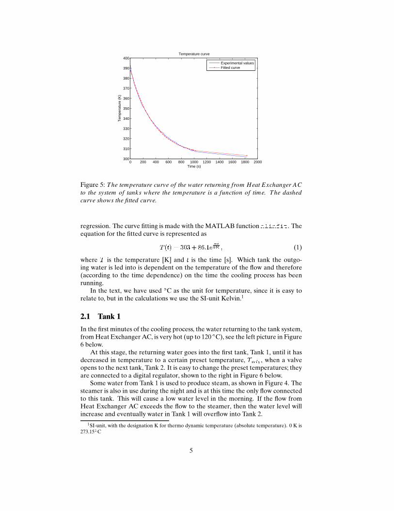
Since the water in the autoclaves gets cooler during the 35 minutes coolingprocess, the streamCSout is warmer at the beginning of the process than towardsthe end. Hence, the temperature of this outgoing stream can be described as afunction of time, plotted in Figure 5. One curve in the figure is plotted withexperimental values on CSout that we measured and the other curve is fitted by

4

0 200 400 600 800 1000 1200 1400 1600 1800 2000300

310

320

330

340

350

360

370

380

390

400Temperature curve

Time (s)

Tem

pera

ture

(K

)

Experimental valuesFitted curve

Figure 5: The temperature curve of the water returning from Heat Exchanger AC

to the system of tanks where the temperature is a function of time. The dashed

curve shows the fitted curve.

regression. The curve fitting is made with the MATLAB function nlinfit. Theequation for the fitted curve is represented asT (t) = 303 + 86:1e �t370 ; (1)

where T is the temperature [K] and t is the time [s]. Which tank the outgo-ing water is led into is dependent on the temperature of the flow and therefore(according to the time dependence) on the time the cooling process has beenrunning.

In the text, we have used ÆC as the unit for temperature, since it is easy torelate to, but in the calculations we use the SI-unit Kelvin.1

2.1 Tank 1

In the first minutes of the cooling process, the water returning to the tank system,from Heat Exchanger AC, is very hot (up to 120 ÆC), see the left picture in Figure6 below.

At this stage, the returning water goes into the first tank, Tank 1, until it hasdecreased in temperature to a certain preset temperature, Tset1 , when a valveopens to the next tank, Tank 2. It is easy to change the preset temperatures; theyare connected to a digital regulator, shown to the right in Figure 6 below.

Some water from Tank 1 is used to produce steam, as shown in Figure 4. Thesteamer is also in use during the night and is at this time the only flow connectedto this tank. This will cause a low water level in the morning. If the flow fromHeat Exchanger AC exceeds the flow to the steamer, then the water level willincrease and eventually water in Tank 1 will overflow into Tank 2.

1SI-unit, with the designation K for thermo dynamic temperature (absolute temperature). 0 K is273.15ÆC

5

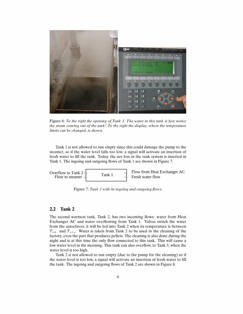
Figure 6: To the right the opening of Tank 1. The water in this tank is hot; notice

the steam coming out of the tank! To the right the display, where the temperature

limits can be changed, is shown.

Tank 1 is not allowed to run empty since this could damage the pump to thesteamer, so if the water level falls too low, a signal will activate an insertion offresh water to fill the tank. Today, the net loss in the tank system is inserted inTank 1. The ingoing and outgoing flows of Tank 1 are shown in Figure 7.

Tank 1Overflow to Tank 2Flow to steamer

Flow from Heat Exchanger AC Fresh water flow

Figure 7: Tank 1 with its ingoing and outgoing flows.

2.2 Tank 2

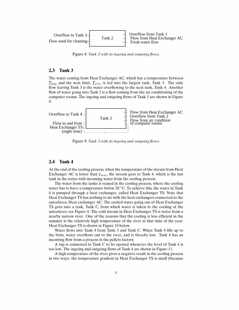
The second warmest tank, Tank 2, has two incoming flows: water from HeatExchanger AC and water overflowing from Tank 1. Valves switch the waterfrom the autoclaves; it will be led into Tank 2 when its temperature is betweenTset1 and Tset2 . Water is taken from Tank 2 to be used in the cleaning of thefactory, even the part that produces pellets. The cleaning is also done during thenight and is at this time the only flow connected to this tank. This will cause alow water level in the morning. This tank can also overflow, to Tank 3, when thewater level is too high.

Tank 2 is not allowed to run empty (due to the pump for the cleaning) so ifthe water level is too low, a signal will activate an insertion of fresh water to fillthe tank. The ingoing and outgoing flows of Tank 2 are shown in Figure 8.

6

Tank 2Flow used for cleaning

Overflow to Tank 3 Overflow from Tank 1Flow from Heat Exchanger ACFresh water flow

Figure 8: Tank 2 with its ingoing and outgoing flows.

2.3 Tank 3

The water coming from Heat Exchanger AC, which has a temperature betweenTset2 and the next limit, Tset3 , is led into the largest tank, Tank 3. The onlyflow leaving Tank 3 is the water overflowing to the next tank, Tank 4. Anotherflow of water going into Tank 3 is a flow coming from the air conditioning of thecomputer rooms. The ingoing and outgoing flows of Tank 3 are shown in Figure9.

Tank 3 Overflow from Tank 2

Flow to and from

(night time)

Overflow to Tank 4

Flow from air condition of computer rooms

Flow from Heat Exchanger AC

Heat Exchanger TS

Figure 9: Tank 3 with its ingoing and outgoing flows.

2.4 Tank 4

At the end of the cooling process, when the temperature of the stream from HeatExchanger AC is lower than Tset3 , the stream goes to Tank 4, which is the lasttank in the series with incoming water from the cooling process.

The water from the tanks is reused in the cooling process, where the coolingwater has to have a temperature below 20 ÆC. To achieve this, the water in Tank4 is pumped through a heat exchanger, called Heat Exchanger TS. Note thatHeat Exchanger TS has nothing to do with the heat exchangers connected to theautoclaves, Heat exchanger AC. The cooled water going out of Heat ExchangerTS goes into a tank, Tank C, from which water is taken to the cooling of theautoclaves; see Figure 4. The cold stream in Heat Exchanger TS is water from anearby narrow river. One of the reasons that the cooling is less efficient in thesummer is the relatively high temperature of the river at that time of the year.Heat Exchanger TS is shown in Figure 10 below.

Water flows into Tank 4 from Tank 3 and Tank C. When Tank 4 fills up tothe brim, water overflows out to the river, and is thereby lost. Tank 4 has anincoming flow from a process in the pellets factory.

A tap is connected to Tank C to be opened whenever the level of Tank 4 istoo low. The ingoing and outgoing flows of Tank 4 are shown in Figure 11.

A high temperature of the river gives a negative result in the cooling processin two ways: the temperature gradient in Heat Exchanger TS is small (because

7

Figure 10: To the left, we can see Heat Exchanger TS and to the right the plates

are visible.

Tank 4 Overflow from Tank 3Flow from pellets factory

Overflow to riverFlow to air condition

of comuter rooms

Overflow from Tank C

Flow from Heat Exchanger ACFlow to Heat Exchanger TS

Figure 11: Tank 4 with its ingoing and outgoing flows.

the temperature difference between the two streams is small), which decreasesthe cooling effect of the water and at the same time algae create an isolatinglayer on the plates in the heat exchanger which decreases its efficiency.

2.5 Tank C

Ideally, the water going out of Heat Exchanger TS into Tank C is below 20 ÆC.As previously stated, this is not always the case, especially in the summer. Thereare several options to lower the temperature of the water going to the coolingprocess; dilution, night cooling and batch; see the next subsections.

A tap is connected to this tank and is opened whenever the level of Tank 4 istoo low, since Tank C overflows into Tank 4. The ingoing and outgoing flows ofTank C are shown in Figure 12.

Tank COverflow to Tank 4 Flow from Heat Exchanger TSFlow to Heat Exchanger AC Fresh water flow

Figure 12: Tank C with its ingoing and outgoing flows.

8

2.5.1 Dilution

A fast option to cool the flow going from Tank C to the Heat Exchanger AC isto dilute it with cold fresh water. The fresh water is added directly into the pipeleading to the autoclaves. The result is an immediate lowering of the tempera-ture, but it can be necessary to add large amounts of fresh water.

2.5.2 Night cooling

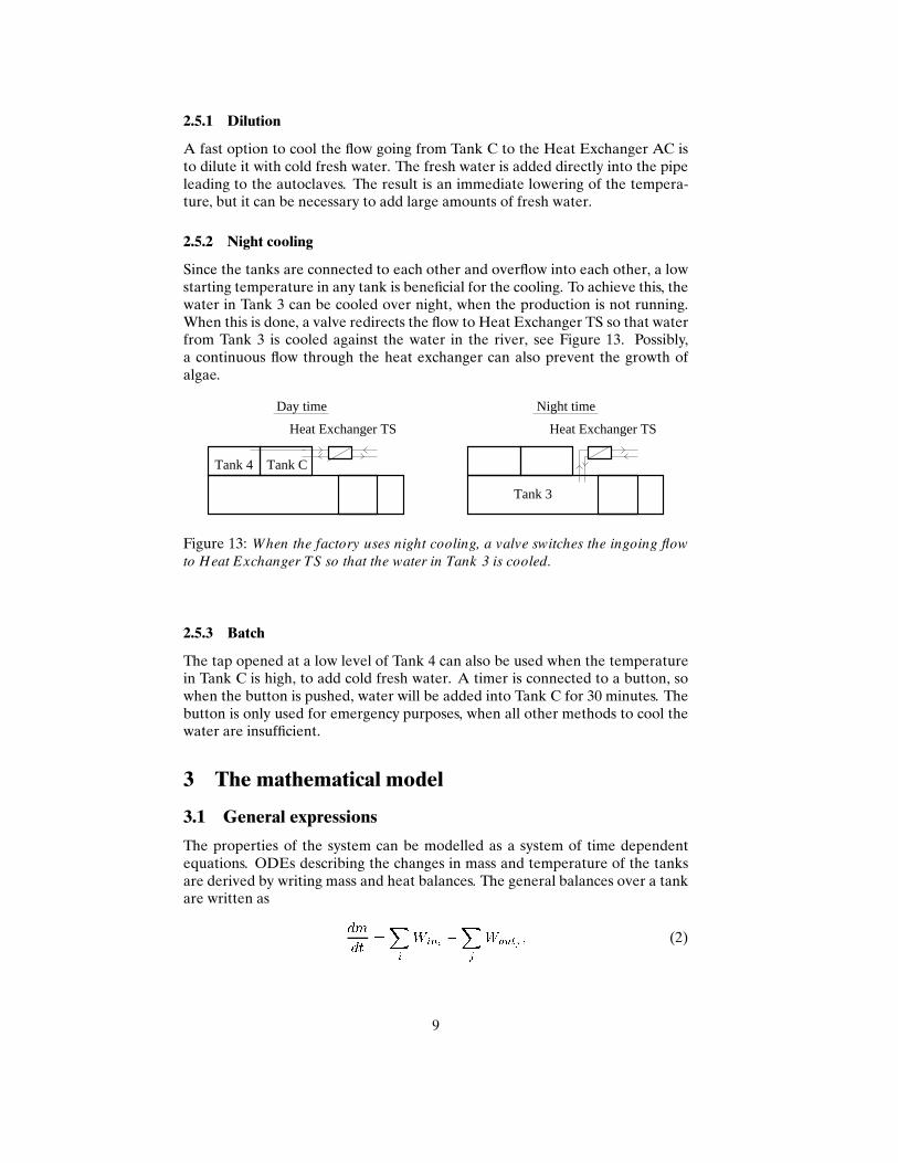
Since the tanks are connected to each other and overflow into each other, a lowstarting temperature in any tank is beneficial for the cooling. To achieve this, thewater in Tank 3 can be cooled over night, when the production is not running.When this is done, a valve redirects the flow to Heat Exchanger TS so that waterfrom Tank 3 is cooled against the water in the river, see Figure 13. Possibly,a continuous flow through the heat exchanger can also prevent the growth ofalgae.

Tank 3

Day time

Heat Exchanger TS

Night time

Heat Exchanger TS

Tank CTank 4

Figure 13: When the factory uses night cooling, a valve switches the ingoing flow

to Heat Exchanger TS so that the water in Tank 3 is cooled.

2.5.3 Batch

The tap opened at a low level of Tank 4 can also be used when the temperaturein Tank C is high, to add cold fresh water. A timer is connected to a button, sowhen the button is pushed, water will be added into Tank C for 30 minutes. Thebutton is only used for emergency purposes, when all other methods to cool thewater are insufficient.

3 The mathematical model

3.1 General expressions

The properties of the system can be modelled as a system of time dependentequations. ODEs describing the changes in mass and temperature of the tanksare derived by writing mass and heat balances. The general balances over a tankare written as dmdt =Xi Wini �Xj Woutj ; (2)

9

dTdt = PiWini(Tini � T )m ; (3)

wherePiWini and

Pj Woutj are the sums of water flows going in and out of thetank, Tini is the temperature of the i:th ingoing flow and T is the temperature ofthe water in the tank. The derivation of the heat balance equation is shown inAppendix A; the derivation of the mass balance equation is analogous.

If equation (2) is divided by �A it can be rewritten asdhdt = PiWini �Pj Woutj�A ; (4)

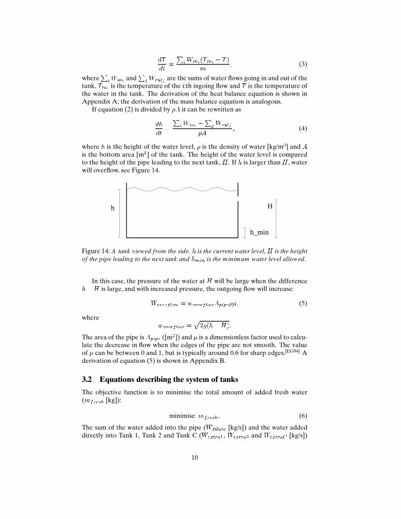
where h is the height of the water level, � is the density of water [kg/m3℄ and Ais the bottom area [m2] of the tank. The height of the water level is comparedto the height of the pipe leading to the next tank, H . If h is larger than H , waterwill overflow, see Figure 14.

h

h_min

H

Figure 14: A tank viewed from the side. h is the current water level, H is the height

of the pipe leading to the next tank and hmin is the minimum water level allowed.

In this case, the pressure of the water at H will be large when the differenceh�H is large, and with increased pressure, the outgoing flow will increase:Woverflow = woverflowApipe��; (5)

where woverflow =p2g(h�H):The area of the pipe is Apipe ([m2]) and � is a dimensionless factor used to calcu-late the decrease in flow when the edges of the pipe are not smooth. The valueof � can be between 0 and 1, but is typically around 0.6 for sharp edges.[EG94] Aderivation of equation (5) is shown in Appendix B.

3.2 Equations describing the system of tanks

The objective function is to minimise the total amount of added fresh water(mfresh [kg]):

minimise mfresh: (6)

The sum of the water added into the pipe (Wdilute [kg/s]) and the water addeddirectly into Tank 1, Tank 2 and Tank C (Wextra1, Wextra2 and WextraC [kg/s])

10

gives the total amount of fresh water added to the system from a given startingtime, �0, to some finite time � :mfresh = Z �t=�0(Wdilute +Wextra1 +Wextra2 +WextraC) dt: (7)

The necessary mass flow of water to add in the pipe at a too high temperaturecan be calculated as Wdilute = Wa Ta �WCoutTCTfresh ; (8)

where Wa [kg/s] is the flow needed in the cooling process (illustrated as WSinin Figure 3), Ta [K] is the temperature of this flow, WCout [kg/s] is the mass flowpumped from Tank C, TC [K] is the temperature of Tank C, and Tfresh [K] is thetemperature of the fresh water.

To get a fast enough cooling of the autoclaves, there is a certain demand ofcooling water. The demand from the autoclaves for the aluminium tins (Da tin[kg/s]) is different from the demand from the Tetra Pak autoclaves (Da tetra[kg/s]). The demands are calculated assuming a fixed number of boilings perhour, and the flow to the autoclaves is assumed to be exactly the demand:Wa = Da tin +Da tetra ; (9)

where Wa = Wdilute +WCout: (10)

Equations (2) and (3) are used to calculate the mass and heat balances forTank C and give dmCdt = W ool �WC4 �WCout +Wextra; (11)dTCdt = W ool(T oolout � TC) +Wextra(Tfresh � TC)mC ; (12)

where W ool [kg/s] is the flow of water going through Heat Exchanger TS andWC4 [kg/s] is the water flow overflowing from Tank C to Tank 4. T oolout [kg/s]is the temperature of the outgoing water from Heat Exchanger TS.

There are no exact relations between the in- and outgoing temperatures andflows for plate heat exchangers that can be used in our simulations. The modelfor Heat Exchanger TS is therefore derived from calculations done by AlfaLaval. How the simulations of the heat exchanger are done is unfortunatelynot known to us, since the simulation programs are confidential. Alfa Laval’s re-sults are calculated with variable values of the flow of the warm stream (which iscalled W ool, since it is the water used to cool the autoclaves). The values of theflow of the cold stream and of the ingoing temperature are kept constant in eachsimulation, but some different cases, with different values on these parameters,are tested.[Las05] The equation for the temperature of the outgoing cooling water,calculated via curve fitting, isT oolout = 287 + (0:0271Tin � 7:8128)W ool: (13)

11

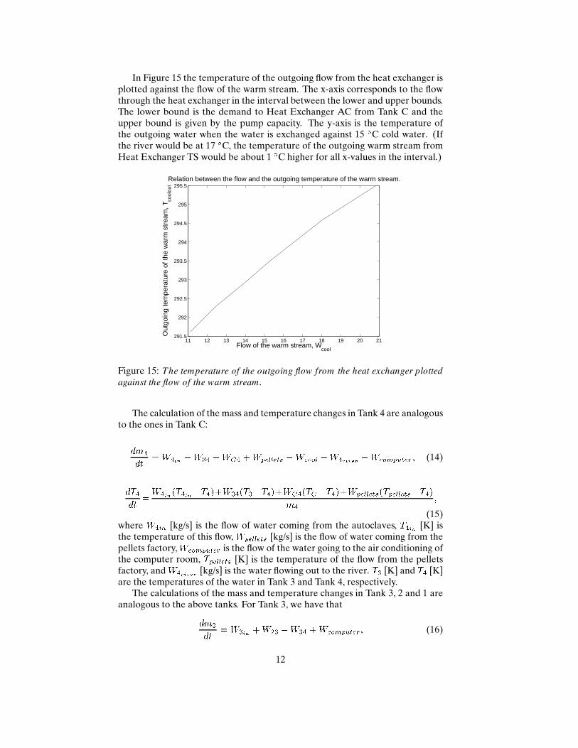
In Figure 15 the temperature of the outgoing flow from the heat exchanger isplotted against the flow of the warm stream. The x-axis corresponds to the flowthrough the heat exchanger in the interval between the lower and upper bounds.The lower bound is the demand to Heat Exchanger AC from Tank C and theupper bound is given by the pump capacity. The y-axis is the temperature ofthe outgoing water when the water is exchanged against 15 ÆC cold water. (Ifthe river would be at 17 ÆC, the temperature of the outgoing warm stream fromHeat Exchanger TS would be about 1 ÆC higher for all x-values in the interval.)

11 12 13 14 15 16 17 18 19 20 21291.5

292

292.5

293

293.5

294

294.5

295

295.5

Flow of the warm stream, Wcool

Out

goin

g te

mpe

ratu

re o

f the

war

m s

trea

m, T

cool

out

Relation between the flow and the outgoing temperature of the warm stream.

Figure 15: The temperature of the outgoing flow from the heat exchanger plotted

against the flow of the warm stream.

The calculation of the mass and temperature changes in Tank 4 are analogousto the ones in Tank C:dm4dt = W4in +W34 +WC4 +Wpellets �W ool �W4river �W omputer ; (14)dT4dt =W4in(T4in�T4)+W34(T3�T4)+WC4(TC�T4)+Wpellets(Tpellets�T4)m4 ;

(15)where W4in [kg/s] is the flow of water coming from the autoclaves, T4in [K] isthe temperature of this flow, Wpellets [kg/s] is the flow of water coming from thepellets factory, W omputer is the flow of the water going to the air conditioning ofthe computer room, Tpellets [K] is the temperature of the flow from the pelletsfactory, and W4river [kg/s] is the water flowing out to the river. T3 [K] and T4 [K]are the temperatures of the water in Tank 3 and Tank 4, respectively.

The calculations of the mass and temperature changes in Tank 3, 2 and 1 areanalogous to the above tanks. For Tank 3, we have thatdm3dt = W3in +W23 �W34 +W omputer; (16)

12

dT3dt = W3in(T3in � T3) +W23(T2 � T3) +W omputer(T5 � T3)m3 : (17)

In the equations for Tank 2, the term describing the flow used in the cleaningof the factory is included (W lean [kg/s]):dm2dt =W2in +W12 +Wextra2 �W lean �W23; (18)dT2dt = W2in(T2in � T2) +W12(T1 � T2) +Wextra2(Tfresh � T2)m2 : (19)

The equations for Tank 1 are analogous to the above calculations, except thatthe hot water from Tank 1 is used for the steamer (Wsteam [kg/s]):dm1dt = W1in +Wextra1 �Wsteam �W12; (20)dT1dt = W1in(T1in � T1) +Wextra1(Tfresh � T1)m1 : (21)

The equations (1)–(21) represent the system as it is today. In this system,Tank 2 runs empty in the evening since a lot of water is used in the cleaningprocess. The low water level gives a low starting temperature in the tank sincefresh water is added to increase the height, which also results in cold cleaningwater. To solve this problem, we take the water for the cleaning process fromTank 3 instead, which will change equations (16) and (18) to:dm3dt = W3in +W23 �W34 +W omputer �W lean +Wextra3 ; (16’)dm2dt =W2in +W12 +Wextra2 �W23: (18’)

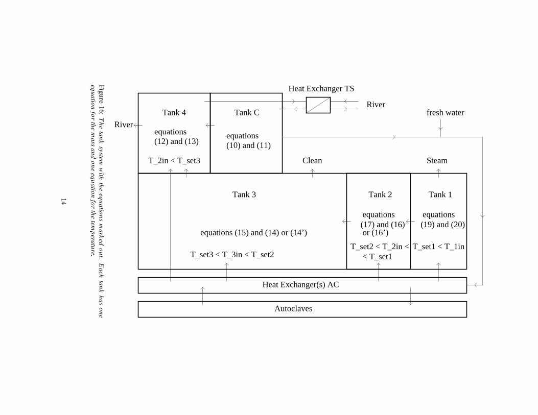
Figure 16 illustrates where each equation belongs in the system. There aretwo equations for every tank, one for the change in mass and one for the changein temperature. Two systems are represented here: the system as it looks to-day and the system where the insertion of fresh water is changes as well as theouttake of the cleaning water.

3.3 Additional constraints

The water level in each tank (hi [m]) is not allowed to ever be below a certainlevel (himin [m]), because the pumps in the system must not run empty:hi � himin ; i = 1; :::; 4: (22)

The flows going through the pumps are limited by the capacities of the pumps(Cpump [kg/s]), which gives upper bounds on W ool and Wfresh:W ool � Cpump ool ; (23)

13

(12) and (13) (10) and (11)

Autoclaves

Tank 2 Tank 1Tank 3

Tank CTank 4

Steam

River

River

Heat Exchanger(s) AC

Heat Exchanger TS

(19) and (20)(17) and (16) or (16’)

T_set3 < T_3in < T_set2

T_2in < T_set3

< T_set1T_set2 < T_2in < T_set1 < T_1in

equations equations

equations (15) and (14) or (14’)

equations equations

Clean

fresh water

Figure16:

Th

eta

nk

system

with

the

equ

atio

ns

ma

rked

ou

t.E

ach

tan

kh

as

on

e

equ

atio

nfo

rth

em

ass

an

do

ne

equ

atio

nfo

rth

etem

pera

ture.

14

Wfresh � Cpumpfresh : (24)

If Tank 4 does not have a low water level, extra water will not be added toTank C; therefore, to guarantee that Tank C is never emptied [see equation (11)],the following constraint is introduced:W ool �WCout;which in combination with equations (9) and (10) gives:Wdilute +W ool � Da tin +Da tetra : (25)

All flows need to be positive:Wj � 0; j 2 J;where J is the set containing all flows in the system.

The water going out from Heat Exchanger AC must go to the different tanksin order, i.e., the water from the cooling must go to Tank 1 first, then to Tank 2,then to Tank 3 and finally to Tank 4; this givesTset1 � Tset2 � Tset3 : (26)

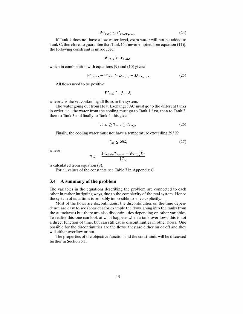
Finally, the cooling water must not have a temperature exceeding 293 K:Ta � 293; (27)

where Ta = WdiluteTfresh +WCoutTCWa is calculated from equation (8).

For all values of the constants, see Table 7 in Appendix C.

3.4 A summary of the problem

The variables in the equations describing the problem are connected to eachother in rather intriguing ways, due to the complexity of the real system. Hencethe system of equations is probably impossible to solve explicitly.

Most of the flows are discontinuous; the discontinuities on the time depen-dence are easy to see (consider for example the flows going into the tanks fromthe autoclaves) but there are also discontinuities depending on other variables.To realise this, one can look at what happens when a tank overflows; this is nota direct function of time, but can still cause discontinuities in other flows. Onepossible for the discontinuities are the flows: they are either on or off and theywill either overflow or not.

The properties of the objective function and the constraints will be discussedfurther in Section 5.1.

15

4 The simulation in Simulink

Since the system of equations is hard to solve, we build a simulation model withthe MATLAB toolbox Simulink. Simulink uses a graphical user interface forbuilding models and making simulations.

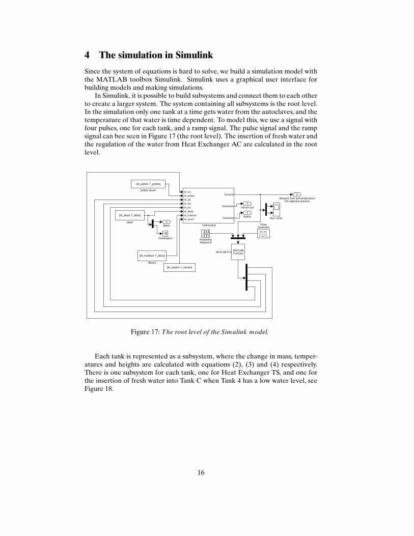
In Simulink, it is possible to build subsystems and connect them to each otherto create a larger system. The system containing all subsystems is the root level.In the simulation only one tank at a time gets water from the autoclaves, and thetemperature of that water is time dependent. To model this, we use a signal withfour pulses, one for each tank, and a ramp signal. The pulse signal and the rampsignal can bee seen in Figure 17 (the root level). The insertion of fresh water andthe regulation of the water from Heat Exchanger AC are calculated in the rootlevel.

4

diltest

3

Button

2

Stream out

1

demand: flow and temperatureThe objective function

[W_pellets T_pellets]

pellets steam

flow ,temp

[W_hotdilute T_dilute]

dilute1

[W_dilute T_dilute]

dilute

Terminator1

W_1in

W_pellets

W_2in

W_3in

W_4in

W_dilute

W_hotdilute

W_riverin

Demand

Streamtest

Buttontest

Tanksystem

RepeatingSequence

PulseGenerator

MATLABFunctionMATLAB Fcn

[W_stream T_stream]

Figure 17: The root level of the Simulink model.

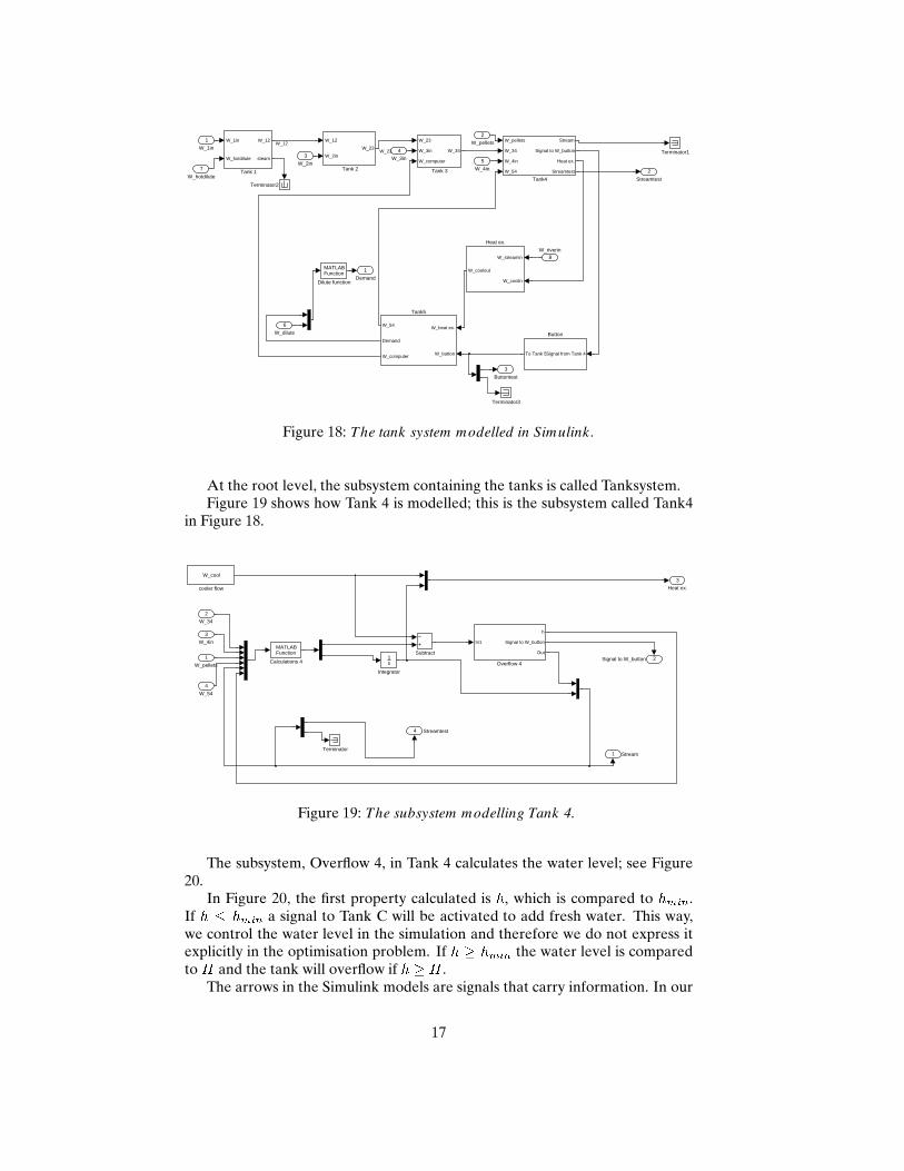
Each tank is represented as a subsystem, where the change in mass, temper-atures and heights are calculated with equations (2), (3) and (4) respectively.There is one subsystem for each tank, one for Heat Exchanger TS, and one forthe insertion of fresh water into Tank C when Tank 4 has a low water level, seeFigure 18.

16

3

Buttontest

2

Streamtest

1

Demand

Terminator3

Terminator2

Terminator1

W_heat ex.

W_button

W_54

Demand

W_computer

Tank5

W_pellets

W_34

W_4in

W_54

Stream

Signal to W_button

Heat ex.

Streamtest

Tank4

W_23

W_3in

W_computer

W_34

Tank 3

W_12

W_2in

W_23

Tank 2

W_1in

W_hotdilute

W_12

steam

Tank 1

W_streamin

W_coolin

W_coolout

Heat ex.

MATLABFunction

Dilute function

Signal from Tank 4To Tank 5

Button

8W_riverin

7

W_hotdilute

6

W_dilute

5

W_4in

4

W_3in3

W_2in

2

W_pellets1

W_1inW_12

W_23

Figure 18: The tank system modelled in Simulink .

At the root level, the subsystem containing the tanks is called Tanksystem.Figure 19 shows how Tank 4 is modelled; this is the subsystem called Tank4

in Figure 18.

4 Streamtest

3

Heat ex.

2Signal to W_button

1 Stream

W_cool

cooler flow

Terminator

Subtract

In1

h

Signal to W_button

Out

Overflow 4 1s

Integrator

MATLABFunction

Calculations 4

4

W_54

3

W_4in

2

W_34

1

W_pellets

Figure 19: The subsystem modelling Tank 4.

The subsystem, Overflow 4, in Tank 4 calculates the water level; see Figure20.

In Figure 20, the first property calculated is h, which is compared to hmin.If h � hmin a signal to Tank C will be activated to add fresh water. This way,we control the water level in the simulation and therefore we do not express itexplicitly in the optimisation problem. If h � hmin the water level is comparedto H and the tank will overflow if h � H .

The arrows in the Simulink models are signals that carry information. In our

17

3

Out

2

Signal to W_button

1

h

1s

int_h Switch1Switch

sqrt

MathFunction

A_pipe*rho*my

Gain4

1/(rho*A4)

Gain

(u−H4)*2*g

Fcn

0 Constant10 Constant

== 0

CompareTo Zero

|u|

Abs

1

In1

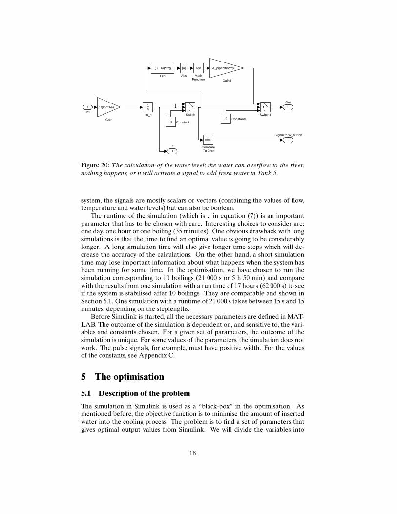
Figure 20: The calculation of the water level; the water can overflow to the river,

nothing happens, or it will activate a signal to add fresh water in Tank 5.

system, the signals are mostly scalars or vectors (containing the values of flow,temperature and water levels) but can also be boolean.

The runtime of the simulation (which is � in equation (7)) is an importantparameter that has to be chosen with care. Interesting choices to consider are:one day, one hour or one boiling (35 minutes). One obvious drawback with longsimulations is that the time to find an optimal value is going to be considerablylonger. A long simulation time will also give longer time steps which will de-crease the accuracy of the calculations. On the other hand, a short simulationtime may lose important information about what happens when the system hasbeen running for some time. In the optimisation, we have chosen to run thesimulation corresponding to 10 boilings (21 000 s or 5 h 50 min) and comparewith the results from one simulation with a run time of 17 hours (62 000 s) to seeif the system is stabilised after 10 boilings. They are comparable and shown inSection 6.1. One simulation with a runtime of 21 000 s takes between 15 s and 15minutes, depending on the steplengths.

Before Simulink is started, all the necessary parameters are defined in MAT-LAB. The outcome of the simulation is dependent on, and sensitive to, the vari-ables and constants chosen. For a given set of parameters, the outcome of thesimulation is unique. For some values of the parameters, the simulation does notwork. The pulse signals, for example, must have positive width. For the valuesof the constants, see Appendix C.

5 The optimisation

5.1 Description of the problem

The simulation in Simulink is used as a “black-box” in the optimisation. Asmentioned before, the objective function is to minimise the amount of insertedwater into the cooling process. The problem is to find a set of parameters thatgives optimal output values from Simulink. We will divide the variables into

18

two different groups: the ones we can control and the ones obtained from thesimulation.

The variables that we are optimising over are the ones we can control:� W ool – the flow through Heat Exchanger TS;� Tset3 – the temperature limit deciding at what temperature the water fromHeat Exchanger AC is led into Tank 4; and� Wdilute – the flow of water added in the pipe to the autoclaves.

These variables are denoted by x. The dimension of x will either be two or three,since we sometimes have a fixed flow of W ool. The variables, x, are constantin time. Another possibility is to have Tset1 and Tset2 as variables, but we havechosen not to, since this makes the problem too large. We have chosen to usethe same temperatures for Tset1 and Tset2 as Doggy uses today: 353 K and 328 Krespectively.

Some of the variables important to us are obtained through the simulation.One of these variables is the flow of water that overflows to the river,W4river , andthe flow inserted to the tanks whenever the water level is too low, Wextrai (i =1; 2; C). The variables, which we cannot control, y, are defined by the set Sim(x).The variables, x, are continuous, but the mapping x 7! Sim(x) is discontinuous.Consider, for example, the case when Wdilute is small; then there will be a largerinsertion of fresh water into Tank C, due to low water levels in Tank 4. Since theinsertion of fresh water is either on or off, Wextra is discontinuous.

The optimisation problem can be written as that to

minimisef(x; y); (28a)

subject to (x; y) � 0; (28b)

q(x; y) = 0; (28c)

a � x � b; (28d)

The inequality constraint (28b) represents the temperature constraint (27).The temperature of the water flow to the autoclaves, Ta , is given by the simula-tion; hence this temperature depends on the simulation results (Ta 2 Sim(x)).The temperature is not allowed to be over 20 ÆC on the entire simulation; theconstraint is expressed as: (x; y) := maxs2S Ta s � 293 � 0: (27’)

If Ta exceeds 293 K, the cooling process will take longer time, but it will notcause any major damage. Therefore, constraint (27’) is ”soft”.

The equality constraints (28c) represent the equations (11)–(21).The lower and upper bounds on x are a and b (equation (28d)). These bounds

are important to fulfill, because the mapping x 7! Sim(x) is undefined outsidesome of the bounds, and because some bounds are set by capacities that cannotbe changed. Hence, the lower and upper bounds are ”hard” constraints.

The system of equations (11)–(21) can be used to express y as a functionof x. Due to the complexity of the system of equations, y is obtained throughthe simulation, which for every given x gives a unique y. Hence we can write

19

y = Sim(x). Important is that the mapping y 7! Sim(x) is defined only when a �x � b. In the optimisation, we do not handle equations (11)–(21) explicitly, sincethey will be calculated and (approximately) fulfilled in the simulation. Thus, weeliminate constraint (28c). When y is substituted with Sim(x), the optimisationproblem can be rewritten as that to

minimise f(x; Sim(x));subject to (x; Sim(x)) � 0;

a � x � b: (29)

We rewrite the problem so that it becomes dependent of x only:

minimise f̂(x);subject to ̂(x) � 0;

a � x � b; (30)

where f̂(x) := f(x; Sim(x)) and ̂(x) := (x; Sim(x)).We have chosen to include the integral of W4river in our objective function

because the water which is lost from the system must sooner or later be replaced.The modified expression for the objective function (6) becomes:f(x) = Z �t=�0(Wdilute +Wextra1+Wextra2+WextraC) dt+ Z �t=�0 W4riverdt: (6’)

The integrals in equation (6’) is substituted with the sum over all time stepsin the simulation: Z �t=�0 W4riverdt �Xs2SW4rivers ;and mfresh = Z �t=�0(Wdilute +Wextra1 +Wextra2 +WextraC) dt �Xs2S(Wdilute +Wextra1 +Wextra2 +WextraC)where S is the set of all time steps in the Simulink simulation.

In Simulink, we use a pulse generator that needs the pulses to have positivewidths. In the calculations, we therefore need to have strict inequalities on con-straint (26). Tset1 and Tset2 are constant in the simulation. We modify constraint(26) to: Tset2 � Tset3 + 4: (26’)

In some of the tanks, there are lower limits for the water levels. These con-straints have been modelled so that water is added to the tanks when the waterlevel sinks below these limits in the simulation. It is possible to model these con-straints so that the algorithm only allows solutions where the water levels neversink too low. Unfortunately, to implement the level constraints in the optimisa-tion has several drawbacks: the algorithm would be much slower, the emergencyadding of water is a better model of how the system works in reality, and most

20

importantly: we might want to see solutions where the level constraints are vi-olated for short periods of time, if the rest of the solution is good. If a levelconstraint is violated, but the solution is good, it is easy to calculate how muchextra water would be needed, and add it to the optimal solution; and maybe stillhave a good solution!

The simulation is used in the objective function; in each step of the iterationthe algorithm evaluates the objective value by running the Simulink model. It isnow obvious that the derivatives of the objective function and of the constraintscannot be calculated analytically; some kind of numerical procedure is necessaryfor the calculation of the gradients and Hessians.

The outcome of the simulation is very sensitive to the values of the constantsand the choice of parameters, as well as the initial values for all the variables,both x and y. Hence, it is of great importance to use accurate initial values.

To test the convexity and the differentiability of the problem, we run thesimulation with different values of Tset3 and Wdilute. The result is shown to theleft in Figure 21, where the objective function is plotted againstWdilute and Tset3.

300

305

310

315

320

0.811.21.41.61.822.22.42.6

3

4

5

6

7

8

9

10

x 104

Tset3

Wdilute

Obj

ectiv

e fu

nctio

n w

ithou

t pen

alty

305

310

315

320

0.811.21.41.61.822.22.42.6

5

5.5

6

6.5

7

7.5

8

8.5

9

9.5

x 104

Tset3

Wdilute

The

obj

ectiv

e fu

nctio

n w

ith p

enal

ty

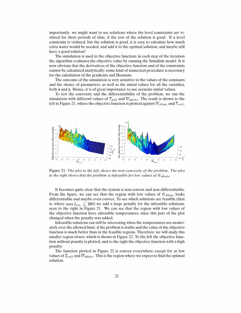
Figure 21: The plot to the left, shows the non-convexity of the problem. The plot

to the right shows that the problem is infeasible for low values of Wdilute.

It becomes quite clear that the system is non-convex and non-differentiable.From the figure, we can see that the region with low values of Wdilute looksdifferentiable and maybe even convex. To see which solutions are feasible (thatis, where maxTa s � 293) we add a large penalty for the infeasible solutions,seen to the right in Figure 21. We can see that the region with low values ofthe objective function have infeasible temperatures, since this part of the plotchanged when the penalty was added.

Infeasible solutions can still be interesting when the temperatures are moder-ately over the allowed limit, if the problem is stable and the value of the objectivefunction is much better than in the feasible regions. Therefore, we will study thissmaller region closer, which is shown in Figure 22. To the left the objective func-tion without penalty is plotted, and to the right the objective function with a highpenalty.

The function plotted in Figure 22 is convex everywhere except for at lowvalues of Tset3 andWdilute. This is the region where we expect to find the optimalsolution.

21

300

305

310

315

320

0.911.11.21.31.41.51.61.71.8

3.5

4

4.5

5

5.5

6

6.5

x 104

Tset3

Wdilute

Obj

ectiv

e fu

nctio

n w

ithou

t pen

alty

300

305

310

315

320

0.811.21.41.61.82

5

6

7

8

9

10

x 104

Tset3

Wdilute

Obj

ectiv

e fu

nctio

n w

ith p

enal

ty

Figure 22: A plot showing that the problem has a region where it is both convex

and differentiable.

For the optimisation, we use MATLAB together with different solvers. Wehave used the built-in MATLAB function fmin on and a software called TOM-LAB with the solvers snopt, onSolve and nlpSolve. The solver fmin onand many of the solvers in TOMLAB are based on the general optimisationmethod of sequential quadratic programming (SQP). SQP and the different solversare described below. If we do not state anything else, the optimisation runs thesystem where the outtake of the water for the cleaning is moved from Tank 2 toTank 3.

5.2 The solvers EGO, rbfSolve and fminsearch

The TOMLAB solver EGO is designed specially for problems that are costly tosolve, for example those that involve simulations, and it does not use derivatives.It would therefore be very well suited for our problem. Another interestingsolver is rbfSolve in TOMLAB. It is, as EGO, designed to find globally opti-mal solutions also for nonconvex optimisation problems and does not requirederivatives. Unfortunately, we do not have licences for these two solvers so weare forced to use some SQP-based solvers.

The solver fminsear h uses a search method, akin to the classic Nelder-Mead algorithm, to find an optimal solution; new iteration points are tried througha procedure that generates trial points conforming to certain geometrical pat-terns. The objective value at a trial point is calculated to see if it is better than thepreviously generated ones. In contrast to SQP, it only uses the objective value tofind the new iteration point. This method needs too many function evaluationsfor our problem, so the running time becomes too long.

5.3 SQP

For solving nonlinearly constrained problems, SQP is a popular method. Theapproach is to find a search direction by solving quadratic programs (problemswith a quadratic function and linear constraints). It is a generalisation of New-ton’s method for unconstrained minimisation. Our problem (30) can be written

22

as:minimisex f̂(x);subject to g(x) � 0; (31)

where

g(x) = 0� ̂(x)�x + a

x� b

1A : (32)

Remember that ̂(x) = maxs2S Ta s � 293.The Lagrangian to problem (31) isL(x;�) = f̂(x)� �T g(x); (33)

where � 2 R2n+1+ (due to the number of constraints: 2n + 1) is the vector ofLagrange multipliers for the constraints (32).

The quadratic programming problem can be written as:

minimisep12pTr2xxL(xk;�k)p +rxL(xk;�k)p;

subject to g(xk) +rg(xk)T p � 0; (34)

where the Lagrange multipliers to the constraints of (34) are denoted by vk.This optimisation problem is a quadratic program, where the quadratic func-tion is a Taylor series approximation of the Lagrangian (33) at (xk;�k) and theconstraints are a linear approximation to g(xk + p) � 0. At each iteration theproblem (34) is solved to obtain (pk; vk) (the search directions for xk and �krespectively), which are used to update (xk;�k). SQP uses a first order Taylorexpansion to replace the nonlinear constraints and uses a second order Taylor se-ries approximation augmented by second order information from the constraintsto replace the nonlinear objective. Our problem does not have analytical deriva-tives and is not differentiable at every point, so the information required forSQP is difficult to obtain. Because of this, SQP is not an ideal method for ourproblem. The reason that we use SQP anyway is that most solvers available tous are based on some SQP algorithm. In all our calculations, derivatives are cal-culated numerically if possible. The calculation of the derivatives are calculatedautomatically in TOMLAB.[AEP05][NS96]

The advantage with SQP is that it uses more information about the objectivefunction when it choses a new search direction. In contrast to fminsear h,to induce convergence, SQP updates the iteration step with a line search ina penalty function which is a linear combination of the objective function andsome measure of the constraint violation.[nlp05]

5.4 The built-in MATLAB function fmincon

One of the solvers we use is the built-in MATLAB function fmin on. Thefunction fmin on uses an SQP algorithm with a penalty function for the con-straints. At every iteration a QP subproblem is solved; the Hessian of the La-grangian is estimated and updated at every iteration similarly to quasi-Newtonmethods.[MaW05b] The penalty function used in fmin on is added to the objectivefunction to form: �(x) = f̂(x) + 2n+1Xi=1 'imaxf0; gi(x)g;

23

where 'i is a penalty parameter, initially set to'i = jjrf̂(x0)jjjjrgi(x0)jj ;and which is updated in each step of the algorithm. The values in x0) are thestarting points. The objective function f̂(x) and the constraint functions gi(x)are required to be continuous, which we cannot guarantee that our functions are.fmin on guarantees to find only stationary points, that is, KKT points. [Mat99]

5.5 The TOMLAB solver snopt

The solver snopt solves nonlinearly constrained problems like our problem(31). It uses an SQP algorithm that exploits the sparsity of the Jacobian of thenonlinear constraints. In our problem (30), the variables y = Sim(x) are nonlin-early dependent on x and cause many nonlinear constraints. We cannot say withcertainty that the Jacobian of (30) is sparse.

5.6 The TOMLAB solver conSolve

The TOMLAB solver onSolve also uses an SQP algorithm. The optimisa-tion problem is written as problem (31) with the Lagrangian function (33). Thepenalty function for the problem with inequalities is:f̂(x)� 2n+1Xi=1 �iui log(ui � gi(x));where u is a vector of barrier parameters.[MaW05a]

We are interested in slightly infeasible solutions, and the barrier functionused in onSolve is very strict on the constraints, since it uses an interior pointpenalty function.

5.7 The TOMLAB solver nlpSolve

Another solver in TOMLAB is nlpSolve, which also uses SQP, but with a dif-ferent approach to fulfill the constraints: it uses a filter instead of a penalty func-tion. Our optimisation problem (31) can be seen as two conflicting minimisationproblems: one is to minimise the objective function and one is to minimise somefunction of the constraint violation. It is written as the multiobjective optimisa-tion program:

minimisex f̂(x)andminimisex w(x); (35)

where w(x) = P2n+1i=1 maxf0; gi(x)g. The filter is a list of pairs of f̂(xk) andw(xk), defined by iterates xk, such that for no pairs, (xk; xl) the following is true:f̂(xk) � f̂(xl), w(xk) � w(xl): if this is the case, we say that no pair dominatesanother pair.

24

At each iteration step of nlpSolve, the new point, xk+1, is accepted if andonly if the corresponding pair (f̂(xk+1) and w(xk+1)) is not dominated by anypair in the filter. If the point is accepted it is included in the filter, and all pointsin the previous filter, that are dominated by the new point, will be rejected.If the point is rejected, the region where the algorithm searches for points isdecreased.[nlp05]

The advantage of nlpSolve for our problem is that the filter can allow someviolation of the nonlinear constraint. An important drawback with nlpSolvefor our problem is that it evaluates the objective function many times, which isextremely time consuming.

6 Results

In this section, the results for the various solvers are presented. The solvers arecompared for three different cases: a constant value on the flow through theHeat Exchanger TS, W ool, with and without night cooling, and a variable W oolwith night cooling.

Tank 1 and Tank 3 have low initial values, since water is used during thenight for the cleaning and for the steamer. The low levels can be interpreted asa deficit of water in the system, which causes low levels in Tank 4. Thus, lowstarting levels in some tanks will inevitably cause water to be added into TankC. An interesting part of the analysis of the results is that of the total amountof water missing in the system. The total mass of this ”missing water” in themorning is: mmissing = msteam +m lean = 24 500 kg

where msteam = (Wsteam � 3 600 � 7);m lean = (W lean � 3 600 � 7):If the tanks are assumed to be full at the end of the day (which they should

be under normal circumstances), it is possible to calculate the initial water levelsof Tank 1 and Tank 3 (h1init and h3init):h1init = H1 � msteamA1� = H1 � 0:1;and h3init = H3 � m leanA3� = H3 � 0:53:These values of h1init and h3init are used as initial values of h1 and h3.

During the day, Wsteam and W lean are taken out from the system. The totalloss of water during the 10 first boilings ismloss = (Wsteam +W lean) � 21 000 = 19 525 kg:

Due to the water used in the cleaning and in the steamer, a total mass ofmmissing +mloss = 44 025 kg can be regarded as necessary to add to the system.If some water is lost to the river (W4river 6= 0), more water has to be added.Hence, to get a low value on W4river is important.

25

If nothing else is stated, we have used the following starting values on thevariables: W ool = 17.5 kg/s (only used when W ool is a variable)Wdilute = 1.11 kg/sTset3 = 308 K

Simulink run time = 21 000 s

When W ool is a constant it is set to its upper bound, 20.3 kg/s. This value ischosen because it is the value Doggy uses today.

The initial values on the tanks are as follows:

Tank i 1 2 3 4 Cwith night without night

cooling coolingTi [K] 363 343 295 328 313 295hi [m] H1 � 1 = 1.7 H2 = 2.6 H3 � 0:53 = 1.97 H4 = 2.7 HC = 2.6

When we solve the problem with fmin on, the built-in penalty function fornon linear constraints do not work very well; the algorithm terminates beforeit had changed any values. We therefore implement a penalty function. To theobjective function, we add the termXs2S 500(maxf0; Ta s � 293g)2: (36)

To be consistent, we try to implement the same penalty in the other solvers, butthis do not work; the algorithms terminate without changing any values. Thedrawback with setting our own penalty is that the penalty parameter will not beupdated by the algorithm.

We have chosen to present the results from fmin on together with the re-sults from the other solvers. However, due to the differences in the penalty func-tion between fmin on and the other solvers, great care should be taken whenthe results are analysed. Whether the built-in or our penalty is used is stated inthe tables.

The value of the objective function is shown in the tables below, togetherwith the values of the corresponding variables and the runtime of the algorithm.

6.1 Optimisation

The results from the optimisation of the system with fixed W ool and with nightcooling are shown in Table 1 for the solvers fmin on, snopt, onSolve andnlpSolve. Figure 23 shows the strong connection between Ta [K], h4 [m] andmextra [kg] (plotted against time); when the water level in Tank 4 is low, extrafresh water is added and therefore Ta is lowered. mextra is the flow Wextramultiplied with the timestep. The results plotted in Figure 23 are obtained fromfmin on.

26

0 1 2

x 104

289

290

291

292

293

294

295

Tac

0 1 2

x 104

0.5

1

1.5

2

2.5

3

h4

0 1 2

x 104

0

50

100

150

200

250

300Extra water into Tank C

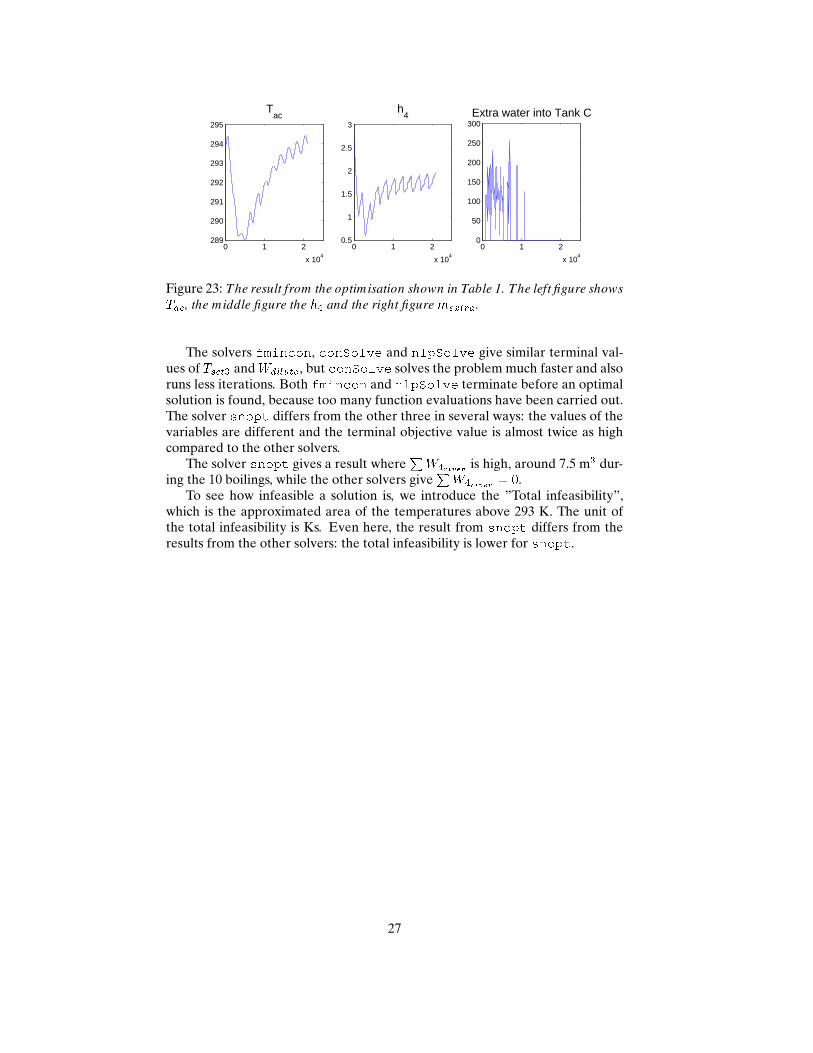
Figure 23: The result from the optimisation shown in Table 1. The left figure showsTa , the middle figure the h4 and the right figure mextra.

The solvers fmin on, onSolve and nlpSolve give similar terminal val-ues of Tset3 and Wdilute, but onSolve solves the problem much faster and alsoruns less iterations. Both fmin on and nlpSolve terminate before an optimalsolution is found, because too many function evaluations have been carried out.The solver snopt differs from the other three in several ways: the values of thevariables are different and the terminal objective value is almost twice as highcompared to the other solvers.

The solver snopt gives a result wherePW4river is high, around 7.5 m3 dur-

ing the 10 boilings, while the other solvers givePW4river = 0.

To see how infeasible a solution is, we introduce the ”Total infeasibility”,which is the approximated area of the temperatures above 293 K. The unit ofthe total infeasibility is Ks. Even here, the result from snopt differs from theresults from the other solvers: the total infeasibility is lower for snopt.

27

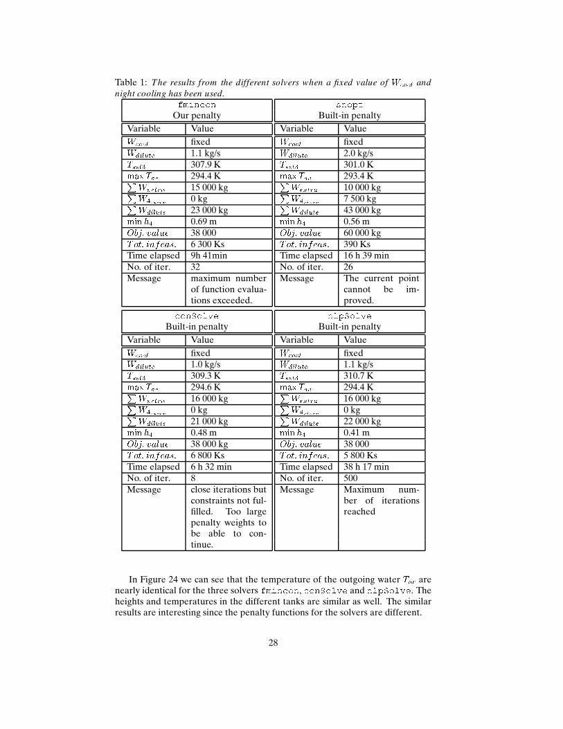
Table 1: The results from the different solvers when a fixed value of W ool and

night cooling has been used.fmin onOur penalty

Variable ValueW ool fixedWdilute 1.1 kg/sTset3 307.9 KmaxTa 294.4 KPWextra 15 000 kgPW4river 0 kgPWdilute 23 000 kgmin h4 0.69 mObj: value 38 000Tot: infeas: 6 300 KsTime elapsed 9h 41minNo. of iter. 32Message maximum number

of function evalua-tions exceeded.

snoptBuilt-in penalty

Variable ValueW ool fixedWdilute 2.0 kg/sTset3 301.0 KmaxTa 293.4 KPWextra 10 000 kgPW4river 7 500 kgPWdilute 43 000 kgmin h4 0.56 mObj: value 60 000 kgTot: infeas: 390 KsTime elapsed 16 h 39 minNo. of iter. 26Message The current point

cannot be im-proved. onSolve

Built-in penaltyVariable ValueW ool fixedWdilute 1.0 kg/sTset3 309.3 KmaxTa 294.6 KPWextra 16 000 kgPW4river 0 kgPWdilute 21 000 kgmin h4 0.48 mObj: value 38 000 kgTot: infeas: 6 800 KsTime elapsed 6 h 32 minNo. of iter. 8Message close iterations but

constraints not ful-filled. Too largepenalty weights tobe able to con-tinue.

nlpSolveBuilt-in penalty

Variable ValueW ool fixedWdilute 1.1 kg/sTset3 310.7 KmaxTa 294.4 KPWextra 16 000 kgPW4river 0 kgPWdilute 22 000 kgmin h4 0.41 mObj: value 38 000Tot: infeas: 5 800 KsTime elapsed 38 h 17 minNo. of iter. 500Message Maximum num-

ber of iterationsreached

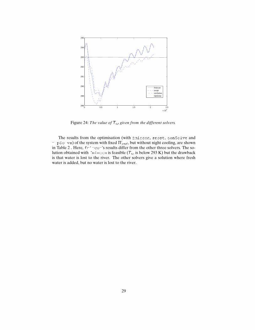
In Figure 24 we can see that the temperature of the outgoing water Ta arenearly identical for the three solvers fmin on, onSolve and nlpSolve. Theheights and temperatures in the different tanks are similar as well. The similarresults are interesting since the penalty functions for the solvers are different.

28

0 0.5 1 1.5 2 2.5

x 104

288

289

290

291

292

293

294

295

fminconsnoptconSolvenlpSolve

Figure 24: The value of Ta given from the different solvers.

The results from the optimisation (with fmin on, snopt, onSolve andnlpSolve) of the system with fixed W ool, but without night cooling, are shownin Table 2 . Here, fmin on’s results differ from the other three solvers. The so-lution obtained with fmin on is feasible (Ta is below 293 K) but the drawbackis that water is lost to the river. The other solvers give a solution where freshwater is added, but no water is lost to the river.

29

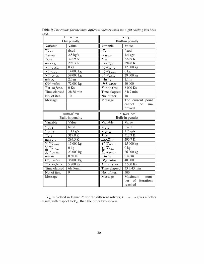
Table 2: The results for the three different solvers when no night cooling has been

used. fmin onOur penalty

Variable ValueW ool fixedWdilute 2.8 kg/sTset3 322.9 KmaxTa 292.3 KPWextra 0 kgPW4river 14 000 kgPWdilute 59 000 kgminh4 2.0 mObj: value 72 000 kgTot: infeas: 0 KsTime elapsed 2h 38 minNo. of iter. 10Message

snoptBuilt-in penalty

Variable ValueW ool fixedWdilute 1.4 kg/sTset3 322.9 KmaxTa 294.8 KPWextra 12 000 kgPW4river 0 kgPWdilute 29 000 kgmin h4 1.1 mObj: value 40 000Tot: infeas: 8 000 KsTime elapsed 8 h 7 minNo. of iter. 18Message The current point

cannot be im-proved onSolve

Built-in penaltyVariable ValueW ool fixedWdilute 1.1 kg/sTset3 317.8 KmaxTa 295.5 KPWextra 15 000 kgPW4river 0 kgPWdilute 23 000 kgminh4 0.80 mObj: value 38 000 kgTot: infeas: 5 200 KsTime elapsed 6h 56minNo. of iter. 9Message

nlpSolveBuilt-in penalty

Variable ValueW ool fixedWdilute 1.2 kg/sTset3 312.3 KmaxTa 295.7 KPWextra 15 000 kgPW4river 0 kgPWdilute 26 000 kgmin h4 0.49 mObj: value 40 000Tot: infeas: 3 500 KsTime elapsed 33 h 43 minNo. of iter. 500Message Maximum num-

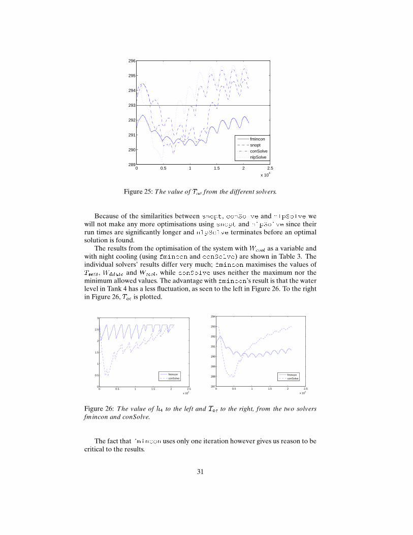
ber of iterationsreachedTa is plotted in Figure 25 for the different solvers; fmin on gives a better

result, with respect to Ta , than the other two solvers.

30

0 0.5 1 1.5 2 2.5

x 104

289

290

291

292

293

294

295

296

fminconsnoptconSolvenlpSolve

Figure 25: The value of Ta from the different solvers.

Because of the similarities between snopt, onSolve and nlpSolve wewill not make any more optimisations using snopt and nlpSolve since theirrun times are significantly longer and nlpSolve terminates before an optimalsolution is found.

The results from the optimisation of the system with W ool as a variable andwith night cooling (using fmin on and onSolve) are shown in Table 3. Theindividual solvers’ results differ very much; fmin on maximises the values ofTset3, Wdilute and W ool, while onSolve uses neither the maximum nor theminimum allowed values. The advantage with fmin on’s result is that the waterlevel in Tank 4 has a less fluctuation, as seen to the left in Figure 26. To the rightin Figure 26, Ta is plotted.

0 0.5 1 1.5 2 2.5

x 104

0

0.5

1

1.5

2

2.5

3

fmincon

conSolve

0 0.5 1 1.5 2 2.5

x 104

287

288

289

290

291

292

293

294

fminconconSolve

Figure 26: The value of h4 to the left and Ta to the right, from the two solvers

fmincon and conSolve.

The fact that fmin on uses only one iteration however gives us reason to becritical to the results.

31

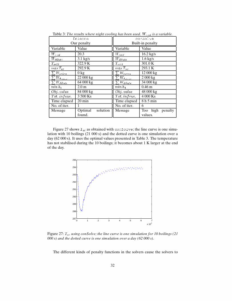
Table 3: The results where night cooling has been used. W ool is a variable.fmin onOur penalty

Variable ValueW ool 20.3Wdilute 3.1 kg/sTset3 322.9 KmaxTa 292.9 KPWextra 0 kgPW4river 22 000 kgPWdilute 64 000 kgminh4 2.0 mObj: value 84 000 kgTot: infeas: 3 500 KsTime elapsed 20 minNo. of iter. 1Message Optimal solution

found.

onSolveBuilt-in penalty

Variable ValueW ool 16.2 kg/sWdilute 1.6 kg/sTset3 301.0 KmaxTa 293.1 KPWextra 12 000 kgPW4river 2 000 kgPWdilute 34 000 kgmin h4 0.46 mObj: value 48 000 kgTot: infeas: 4 000 KsTime elapsed 8 h 5 minNo. of iter. 6Message Too high penalty

values.

Figure 27 shows Ta as obtained with onSolve; the line curve is one simu-lation with 10 boilings (21 000 s) and the dotted curve is one simulation over aday (62 000 s). It uses the optimal values presented in Table 3. The temperaturehas not stabilised during the 10 boilings; it becomes about 1 K larger at the endof the day.

0 1 2 3 4 5 6 7

x 104

287

288

289

290

291

292

293

294

295

Figure 27: Ta using conSolve; the line curve is one simulation for 10 boilings (21

000 s) and the dotted curve is one simulation over a day (62 000 s).

The different kinds of penalty functions in the solvers cause the solvers to

32

work differently. At the first sight, the solvers in TOMLAB seem to allow infea-sible solutions while fmin on prioritise feasibility. However, it is possible thatthe TOMLAB solvers are so sensitive to infeasible solutions that they terminatebefore they have found an optimal solution. fmin on on the other hand, givesa penalty on infeasible solutions, but does not terminate.

We do not get an obvious answer on which Tset3 should be used. The solversgive varying results that seem to depend highly on the other variables. However,there is one trend concerning Tset3: when the level of the water in Tank 4 is low,Tset3 tends to be low, which will result in a larger input of water into Tank 4 fromthe autoclaves.

Most of our solutions are infeasible; the solvers could not find feasible so-lutions. There exist feasible solutions though, since more water can be added,i.e Wdilute can be increased. It is of great interest to see the solutions we haveobtained, since sometimes it can be acceptable to have a too large temperaturefor a short period of time, when it is very expensive to lower it with fresh water.

Most solvers terminate before an optimal solution is found. Therefore thethere might be better solutions for the problem, than the ones stated above.

Because Tank 1 and Tank 3 have low initial levels, Tank 4 is emptied fasterthan the extra water is added. Thus, if the limit where Tank 4 starts to be filledwith extra water is set too low, Tank 4 is emptied. An easy solution to this prob-lem is to set this limit higher. Therefore, we have changed the original setting onh4min from 0.8 meters to 1.5 meters.

The results depend highly on the initial values of the water levels: if Tank1 and Tank 2 have low levels, Tank 4 can be emptied, which will cause a largeflow on WextraC . Important to notice is that the extra water added, due to lowlevels in Tank 4, is not always unnecessary. The levels of Tank 1 and Tank 3 arelow initially because water has been removed from the tanks during the nightfor cleaning and for the steamer. Since this is a loss in the production, replaceinglost water from the system is necessary. One could even think of a way to includethe low levels of the tanks in the objective function.

6.2 Improvements

To see if the changes made of the system have improved it, we run simulationson the ”old” and the ”new” system and compare them. The old system is thesystem as it is today; the insertion of water is to Tank 1 and water to the cleaningis taken from Tank 2. The new system is the system we used in our calculations:the cleaning water is taken from Tank 3 and the fresh water Wdilute is added inthe pipe.

The results from the simulations of the old and the new system, when nightcooling has been used, are shown in Table 4. The values for Tset3 and Wdiluteare taken from the results from fmin on with night cooling (Table 1). The newsystem has two important advantages: the loss to the river is small or zero andTa is lower (that is the total infeasibility is lower).

33

Table 4: A comparison between the old and the new system. With night cooling.

Old systemVariable ValuePWextra 17 000 kgPW4river 0 kgTot: infeas: 32 000 Ks

New systemVariable ValuePWextra 16 000 kgPW4river 0 kgTot: infeas: 5 900 Ks

The values of Ta and h4 (with night cooling) are shown in Figure 28, wherethe values for old system is plotted with the dashed line.

0 0.5 1 1.5 2 2.5

x 104

289

290

291

292

293

294

295

296

297

Tac

0 0.5 1 1.5 2 2.5

x 104

0

0.5

1

1.5

2

2.5

3

h4

Figure 28: Comparisons between the old and the new system. Night cooling has

been used.

The results from the simulations of the two systems, when no night cooling hasbeen used, are shown in Table 5. The values for Tset3 and Wdilute are takenfrom the results from fmin on without night cooling (Table 2). When the nightcooling has not been used, the differences between the systems are even moreobvious. Notice the value of W4river and the total infeasibility for the old system!

Table 5: A comparison between the old and the new system. Without night cooling.

Old systemVariable ValuePWextra 6 600 kgPW4river 35 000 kgTot: infeas: 85 000 Ks

New systemVariable ValuePWextra 0 kgPW4river 13 000 kgTot: infeas: 0 Ks

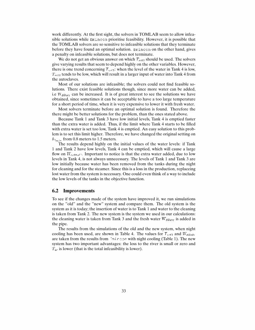
When no night cooling is used, the difference in Ta is remarkably large. Thevalues of Ta and h4 without night cooling are shown in Figure 29. The valuesfor the old system are plotted with the dashed line.The value of Ta is up to 6.5 K lower in the new system compared to the old one.

34

0 0.5 1 1.5 2 2.5

x 104

290

291

292

293

294

295

296

297

298

299

Tac

0 0.5 1 1.5 2 2.5

x 104

0.8

1

1.2

1.4

1.6

1.8

2

2.2

2.4

2.6

2.8

h4

Figure 29: Comparisons between the old and the new system. No night cooling

has been used.

The results from the simulations of the two systems, when night cooling hasbeen used, are shown in Table 6. The values for Tset3 and Wdilute are taken fromthe results from fmin onwith night cooling (Table 3). WhenW ool is a variable,the differences between the systems are even more obvious.

Table 6: A comparison between the old and the new system. With night cooling

and variable W ool.Old system

Variable ValuePWextra 5 800 kgPW4river 47 000 kgTot: infeas: 88 000 Ks

New systemVariable ValuePWextra 0 kgPW4river 21 000 kgTot: infeas: 0 Ks

The values of Ta and h4 without night cooling are shown in Figure 30. Thevalues for the old system are plotted with the dashed line.

The value of Ta is up to 8 K lower, and the water level in Tank 4 is clearlymore stable, in the new system compared to the old one.

0 0.5 1 1.5 2 2.5

x 104

288

290

292

294

296

298

300

Tac

0 0.5 1 1.5 2 2.5

x 104

1

1.2

1.4

1.6

1.8

2

2.2

2.4

2.6

2.8

h4

Figure 30: Comparisons between the old and the new system. Night cooling has

been used.

35

The results from this section show that it is better to insert the fresh water inthe pipe instead of into Tank 1. To do so will lower the temperature 3–8 K. Thewater level in Tank 4 is also more stable in the new system.

To show the effect of the night cooling, the optimal values obtained fromfmin on with fixed W ool and night cooling (Table 1) are used to run two simu-lations: one with and one without night cooling. The values of Ta from the twosimulations are plotted in Figure 31. Night cooling (plotted with the solid line)lowers the temperature with up to 3.5 K.

0 0.5 1 1.5 2 2.5

x 104

288

289

290

291

292

293

294

295

296

297

Tac

Figure 31: The value of Ta , with and without night cooling.

7 Discussion

Tank 1, 2 and 4 are not allowed to run empty since there are pumps there. If thewater level is too low, a signal will start a pump (or, in Tank 4, a tap) that addswater to the tank. When the water reaches a certain level, another signal willclose the tap. In this project, a flow is going to fill the tank as long as the levelis on or below the minimum, but it will stop as soon as the water level goes overthis limit. If the water level is around this height, this is going to make the systemless robust than in reality.

When the water level in a tank reaches a certain level, it will overflow intothe next tank through a pipe in the tank wall. The height of the pipes are dif-ferent for each tank and the water will therefore mostly go to the next tank inline. However, if a tank is full, and the previous tank has a low level, the watercould flow backwards in the system, which would cause the temperature differ-ences between the tanks to decrease. In the simulation this possibility has beenremoved, simply because the calculations become too large and slow. With thelarge amounts of water in the system during our simulations, this effect can beneglected, but in future simulation it may have to be taken into account.

We have assumed that the tanks are perfectly mixed and therefore have thesame temperature throughout the tank. This is not an unreasonable approxima-tion for Tank 1 and Tank 2 because the high temperatures in these tanks causeturbulence. Tank 4 and Tank C can also be considered mixed, since there is alarge exchange of water in these tanks. The tank where the assumption, of per-fectly mixed tanks, is not always correct is Tank 3 where layers of water withdifferent temperatures can occur.

36

A difficulty in this project was that the system includes several plate heatexchangers, both in the tank system and in connection with the autoclaves. Theprinciple of plate heat exchangers (run two streams of water on each side ofa plate) may be quite simple, but the calculations are far from trivial. In fact,there is hardly any literature on the subject and many of the relations used incalculations on plate heat exchangers are based on experiments. Since our modelfor Heat Exchanger TS is derived using such relations and regression, it is onlyan approximation, and even a rather crude one.

Another interesting problem is how to establish the demand of water neededin the cooling process. A first thought was to calculate the demand from theproperties of the autoclaves and the tins. It soon showed that this problem wasvery complex. For example, the properties of plate heat exchangers are not verywell known, and the calculation of the heat transfer from the tins to the waterin the autoclaves is difficult. An important thing to notice is that the demandof cooling water is not a constant value. When the temperature of the coolingwater is low, a smaller flow is sufficient for the cooling, while a higher flow isneeded at higher temperatures. The heat exchangers in the autoclaves also havean effect since they work better at certain flows. Altogether, the calculationsof the demand of cooling water is actually an optimisation problem of its own,and would need more study than is possible in this thesis. Therefore we havemeasured the present flows going to the cooling process and used them in ourcalculations. The production of the Tetra Pak is limited to one boiling per hourwhile there can be about 1.7 boiling of aluminium tins. These limits depend onthe time it takes to fill the autoclaves and boil the tins. In our calculations, wehave assumed the demand of cooling water to the autoclaves to be constant,but this is only true for the Tetra Pak autoclaves. The cooling processes of theoriginal tins occasionally overlap, and then the mass flow of cooling water perautoclave is decreased.

To change the outtake of the cleaning water is beneficial for the system inseveral ways; the temperature of the cleaning water will have a more appropri-ate temperature and will not run out. The change of the cleaning water willaffect the system mainly at night; when cleaning water is used even when theproduction is not running. Hence, this change will not make a big difference inour calculations, since we do not study the behaviour of the system at night.

8 Further possible developments

A future change to make a better cooling of the water can be to consider the sizeof Tank 4. This tank is small and has very large flows which makes it sensitive.One possible improvement is to run the heat exchanger through Tank 3 insteadof Tank 4 and to put the outlet of water to the narrow river in Tank 3. Anotherpossibility is to remove the wall between Tank 3 and Tank 4. This will make thetank larger and more stable, but the temperatures in it would be more difficult tocontrol. Another option to solve the problem with the instability of Tank 4 is tomake one large tank out of Tank 4 and Tank 5. A drawback with making a largetank out of the two, is that the water led to the autoclaves could have a highertemperature.

37

References

[AEP05] N. Andréasson, A. Evgrafov, and M. Patriksson. A n Introduction to

Continuous Optimization. Studentlitteratur, Lund, 2005.

[con05] Tomlab solver consolve, 07112005.http://tomlab.biz/products/base/solvers% textup/conSolve.php.

[EG94] I. Ekroth and E. Granryd. Tillämpad termodynamik . AB GrafiskaGruppen, Stockholm, 1994.

[GMS05] P. Gill, W. Murray, and M. Saunders. Snopt: An sqp algorithm forlarge-scale constrained optimization. SIA M Review, 47(1):99–131,2005.

[Las05] I. Lasson, 2005. Product Manager, Thermal equipment, Alfa Laval.Written communication.

[Mat99] The MathWorks. Optimizatioon toolbox, for use with matlab. 1999.

[MaW05a] The math works, optimization toolbox help, 0312005.http://www.mathworks.com/access/helpdesk/help/toolbox/gads/bqf9jvg-1.html.

[MaW05b] The math works, optimization toolbox help, 07112005.http://www.mathworks.com/access/helpdesk/help/toolbox/optim/ug/.

[NE05] National encyclopedin, 10102005. http://www.ne.se/jsp/search/article.jsp?i_art_id=120909&i_word=autoklav.

[nlp05] Tomlab solver nlpsolve, 04112005.http://www.math.dundee.ac.uk/ ftp/na-reportsup/NA171_RF_SL.ps.

[NS96] S. Nash and A. Sofer. L inear and Nonlinear Programming. McGraw-Hill, Singapore, 1996.

[Pet05] T. Pettersson, 2005. Produktionsteknisk chef, Doggy AB. Oral com-munication.

38

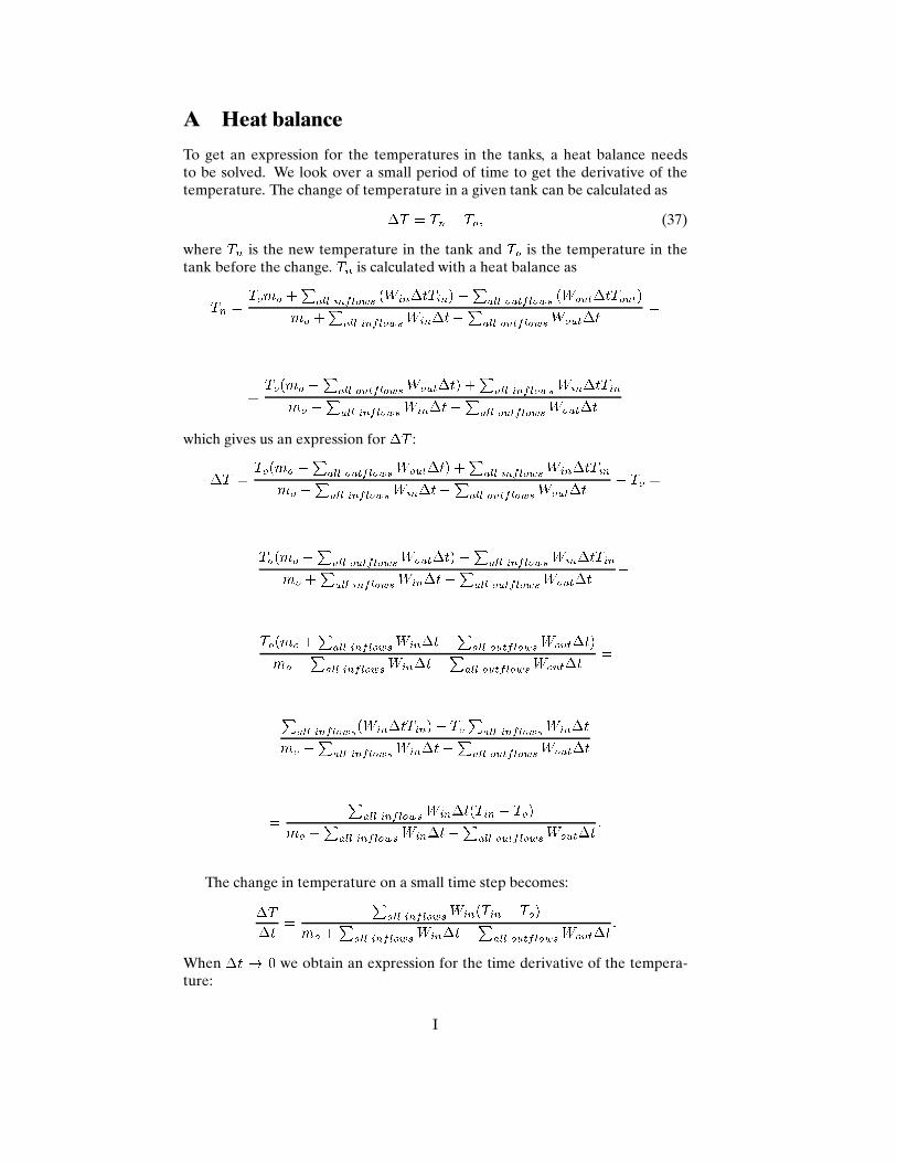
A Heat balance

To get an expression for the temperatures in the tanks, a heat balance needsto be solved. We look over a small period of time to get the derivative of thetemperature. The change of temperature in a given tank can be calculated as�T = Tn � To; (37)

where Tn is the new temperature in the tank and To is the temperature in thetank before the change. Tn is calculated with a heat balance asTn = Tomo +Pall inflows (Win�tTin)�Pall outflows (Wout�tTout)mo +Pall inflowsWin�t�Pall outflowsWout�t =

= To(mo �Pall outflowsWout�t) +Pall inflowsWin�tTinmo +Pall inflowsWin�t�Pall outflowsWout�twhich gives us an expression for �T :�T = To(mo �Pall outflowsWout�t) +Pall inflowsWin�tTinmo +Pall inflowsWin�t�Pall outflowsWout�t � To == To(mo �Pall outflowsWout�t) +Pall inflowsWin�tTinmo +Pall inflowsWin�t�Pall outflowsWout�t �To(mo +Pall inflowsWin�t�Pall outflowsWout�t)mo +Pall inflowsWin�t�Pall outflowsWout�t == Pall inflows(Win�tTin)� ToPall inflowsWin�tmo +Pall inflowsWin�t�Pall outflowsWout�t == Pall inflowsWin�t(Tin � To)mo +Pall inflowsWin�t�Pall outflowsWout�t :

The change in temperature on a small time step becomes:�T�t = Pall inflowsWin(Tin � To)mo +Pall inflowsWin�t�Pall outflowsWout�t :When �t ! 0 we obtain an expression for the time derivative of the tempera-ture:

I

�T�t ������t!0 ) dTdt = Pall inflowsWin(Tin � To)mo (38)

The derivation is analogous for the mass balance of each tank.

B Overflow

The overflow from one tank to another, with the points 1 and 2 in Figure 32 iscalculated with Bernoulli’s equation [EG94]:p1� + w212 + gz1 = p2� + w222 + gz2; (39)

h H

2

1

Figure 32: Bernoulli’s equation is calculated on the two points 1 and 2.

where p is the pressure, w is the velocity and z is the water level, which withp1 = p2, w1 = dhdt , z1 = h, w2 = w2, and z2 = H gives�dhdt �22 + gh = w222 + gH: (40)

If we rewrite this, we have:w22 = 2g(h�H) +�dhdt �2 ; (41)

which gives us an expression for the velocity going out of the hole:w2 =s2g(h�H) +�dhdt �2;where w2 is the velocity of the water going through the hole and dhdt is the change

of the water level in Tank 1, see Figure 32. Since�dhdt �2 << w2 we neglect it, and

the equation becomes: w2 =p2g(h�H)II

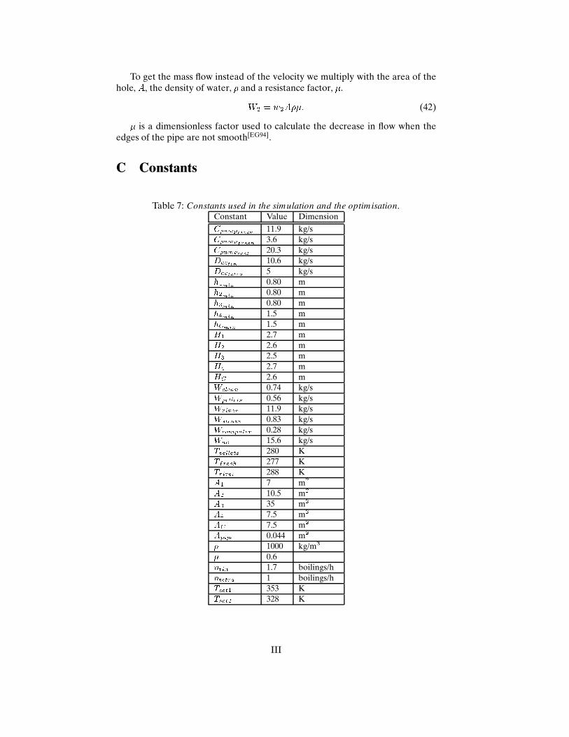
To get the mass flow instead of the velocity we multiply with the area of thehole, A, the density of water, � and a resistance factor, �.W2 = w2A��: (42)� is a dimensionless factor used to calculate the decrease in flow when theedges of the pipe are not smooth[EG94].

C Constants

Table 7: Constants used in the simulation and the optimisation.

Constant Value DimensionCpumpriver 11.9 kg/sCpumpfresh 3.6 kg/sCpump ool 20.3 kg/sDa tin 10.6 kg/sDa tetra 5 kg/sh1min 0.80 mh2min 0.80 mh3min 0.80 mh4min 1.5 mhCmin 1.5 mH1 2.7 mH2 2.6 mH3 2.5 mH4 2.7 mHC 2.6 mW lean 0.74 kg/sWpellets 0.56 kg/sWriver 11.9 kg/sWsteam 0.83 kg/sW omputer 0.28 kg/sWa 15.6 kg/sTpellets 280 KTfresh 277 KTriver 288 KA1 7 m2A2 10.5 m2A3 35 m2A4 7.5 m2AC 7.5 m2Apipe 0.044 m2� 1000 kg/m3� 0.6ntin 1.7 boilings/hntetra 1 boilings/hTset1 353 KTset2 328 K

III

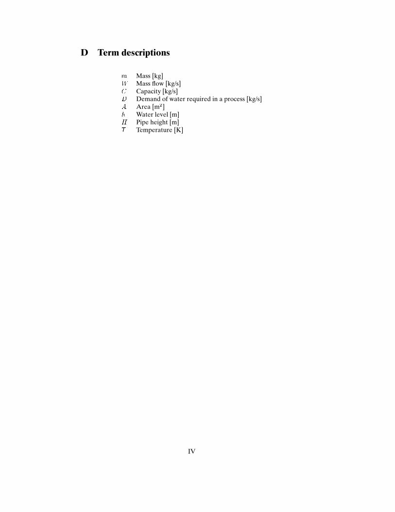
D Term descriptionsm Mass [kg]W Mass flow [kg/s]C Capacity [kg/s]D Demand of water required in a process [kg/s]A Area [m2]h Water level [m]H Pipe height [m]T Temperature [K]

IV