Embed Size (px)
Citation preview
A NUMERICAL VORTEX APPROACH TO AERODYNAMIC
MODELING OF SUAV/VTOL AIRCRAFT
by
Douglas F. Hunsaker
A thesis submitted to the faculty of
Brigham Young University
in partial fulfillment of the requirements for the degree of
Master of Science
Department of Mechanical Engineering
Brigham Young University
April 2007

Copyright c! 2006 Douglas F. Hunsaker
All Rights Reserved

BRIGHAM YOUNG UNIVERSITY
GRADUATE COMMITTEE APPROVAL
of a thesis submitted by
Douglas F. Hunsaker
This thesis has been read by each member of the following graduate committee andby majority vote has been found to be satisfactory.
Date Deryl O. Snyder, Chair
Date Timothy W. McLain
Date Je!rey P. Bons

BRIGHAM YOUNG UNIVERSITY
As chair of the candidate’s graduate committee, I have read the thesis of Douglas F.Hunsaker in its final form and have found that (1) its format, citations, and bibli-ographical style are consistent and acceptable and fulfill university and departmentstyle requirements; (2) its illustrative materials including figures, tables, and chartsare in place; and (3) the final manuscript is satisfactory to the graduate committeeand is ready for submission to the university library.
Date Deryl O. SnyderChair, Graduate Committee
Accepted for the Department
Matthew R. JonesGraduate Coordinator
Accepted for the College
Alan R. ParkinsonDean, Ira A. Fulton College ofEngineering and Technology

ABSTRACT
A NUMERICAL VORTEX APPROACH TO AERODYNAMIC
MODELING OF SUAV/VTOL AIRCRAFT
Douglas F. Hunsaker
Department of Mechanical Engineering
Master of Science
A combined wing and propeller model is presented as a low-cost approach to
preliminary modeling of slipstream e!ects on a finite wing. The wing aerodynamic
model employs a numerical lifting-line method utilizing the 3D vortex lifting law
along with known 2D airfoil data to predict the lift distribution across a wing for
a prescribed upstream flowfield. The propeller/slipstream model uses blade element
theory combined with momentum conservation equations. This model is expected to
be of significant importance in the design of tail-sitter vertical take-o! and landing
(VTOL) aircraft, where the propeller slipstream is the primary source of air flow past
the wings in some flight conditions. The algorithm is presented, and results compared
with published experimental data.


ACKNOWLEDGMENTS
I would like to thank Dr. Snyder for his wise mentoring, guidance, and friend-
ship throughout the progression of this research. Additionally, I’d like to thank my
family members who have supported and encouraged me. Lastly, I’d like to thank
the giants on whose shoulders I have been allowed to stand and from whose research
I have learned and benefited.

Table of Contents
Acknowledgements xi
List of Figures xvii
1 Introduction 1
1.1 Background . . . . . . . . . . . . . . . . . . . . . . . . . . . . . . . . 1
1.2 Objective . . . . . . . . . . . . . . . . . . . . . . . . . . . . . . . . . 3
1.3 Related Work . . . . . . . . . . . . . . . . . . . . . . . . . . . . . . . 3
1.4 Contributions . . . . . . . . . . . . . . . . . . . . . . . . . . . . . . . 4
1.4.1 Resulting Publications . . . . . . . . . . . . . . . . . . . . . . 5
1.5 Thesis Overview . . . . . . . . . . . . . . . . . . . . . . . . . . . . . . 5
2 Numerical Lifting Line Model 7
2.1 Nomenclature . . . . . . . . . . . . . . . . . . . . . . . . . . . . . . . 7
2.2 History . . . . . . . . . . . . . . . . . . . . . . . . . . . . . . . . . . . 9
2.3 Assumptions . . . . . . . . . . . . . . . . . . . . . . . . . . . . . . . . 11
2.3.1 Potential Flow . . . . . . . . . . . . . . . . . . . . . . . . . . 11
2.3.2 2D Airfoil Characteristics At Each Spanwise Wing Section . . 11
2.3.3 Elliptical Lift Distribution Initial Guess . . . . . . . . . . . . . 12
2.4 Formulation . . . . . . . . . . . . . . . . . . . . . . . . . . . . . . . . 12
2.4.1 Overview . . . . . . . . . . . . . . . . . . . . . . . . . . . . . 12
2.4.2 Vortex Strengths . . . . . . . . . . . . . . . . . . . . . . . . . 13
xiii
2.4.3 Aerodynamic Forces and Moments . . . . . . . . . . . . . . . 15
2.5 Solvers . . . . . . . . . . . . . . . . . . . . . . . . . . . . . . . . . . . 16
2.5.1 Linearized System . . . . . . . . . . . . . . . . . . . . . . . . 16
2.5.2 Adjusted Linear Solver . . . . . . . . . . . . . . . . . . . . . . 17
2.5.3 Jacobian Solver . . . . . . . . . . . . . . . . . . . . . . . . . . 18
2.5.4 Picard Solver . . . . . . . . . . . . . . . . . . . . . . . . . . . 19
2.5.5 Steepest Descent Solver . . . . . . . . . . . . . . . . . . . . . 20
2.5.6 BFGS Update Solver . . . . . . . . . . . . . . . . . . . . . . . 21
2.6 Flaps . . . . . . . . . . . . . . . . . . . . . . . . . . . . . . . . . . . . 22
2.6.1 Lift Coe"cient . . . . . . . . . . . . . . . . . . . . . . . . . . 23
2.6.2 Drag Coe"cient . . . . . . . . . . . . . . . . . . . . . . . . . . 25
2.6.3 Moment Coe"cient . . . . . . . . . . . . . . . . . . . . . . . . 25
2.6.4 Flaps Above Stall . . . . . . . . . . . . . . . . . . . . . . . . . 26
2.7 Summary . . . . . . . . . . . . . . . . . . . . . . . . . . . . . . . . . 26
3 Numerical Blade-Element Model 27
3.1 Nomenclature . . . . . . . . . . . . . . . . . . . . . . . . . . . . . . . 27
3.2 History . . . . . . . . . . . . . . . . . . . . . . . . . . . . . . . . . . . 28
3.3 Assumptions . . . . . . . . . . . . . . . . . . . . . . . . . . . . . . . . 29
3.4 Formulation . . . . . . . . . . . . . . . . . . . . . . . . . . . . . . . . 30
3.5 Battery and Motor Properties . . . . . . . . . . . . . . . . . . . . . . 31
3.6 Combined Model Assumptions . . . . . . . . . . . . . . . . . . . . . . 32
4 Results 33
4.1 Lifting Line Model . . . . . . . . . . . . . . . . . . . . . . . . . . . . 33
4.1.1 Below Stall . . . . . . . . . . . . . . . . . . . . . . . . . . . . 33
4.1.2 Above Stall . . . . . . . . . . . . . . . . . . . . . . . . . . . . 34
xiv
4.1.3 NACA 0015 Test Case . . . . . . . . . . . . . . . . . . . . . . 40
4.1.4 Upstream Velocity E!ects . . . . . . . . . . . . . . . . . . . . 41
4.2 Propeller Model . . . . . . . . . . . . . . . . . . . . . . . . . . . . . . 47
4.2.1 Total Thrust . . . . . . . . . . . . . . . . . . . . . . . . . . . 47
4.2.2 Velocity Profiles . . . . . . . . . . . . . . . . . . . . . . . . . . 49
4.2.3 Slipstream Profile . . . . . . . . . . . . . . . . . . . . . . . . . 50
4.3 Combined Models . . . . . . . . . . . . . . . . . . . . . . . . . . . . . 52
5 6 DOF Simulator Application 55
6 Conclusion 61
6.1 Lifting Line Model . . . . . . . . . . . . . . . . . . . . . . . . . . . . 61
6.2 Propeller Model . . . . . . . . . . . . . . . . . . . . . . . . . . . . . . 61
6.3 Combined Models . . . . . . . . . . . . . . . . . . . . . . . . . . . . . 62
6.4 Resulting Software: Aither . . . . . . . . . . . . . . . . . . . . . . . . 62
A Derivation of Lifting-Line Equation 63
A.1 Nomenclature . . . . . . . . . . . . . . . . . . . . . . . . . . . . . . . 63
A.2 Overview of Numerical Lifting Line Method . . . . . . . . . . . . . . 64
A.3 Jacobian . . . . . . . . . . . . . . . . . . . . . . . . . . . . . . . . . . 65
A.4 Linear Approximation . . . . . . . . . . . . . . . . . . . . . . . . . . 69
Bibliography 73
xv

xvi
List of Figures
1.1 The Convair XFY-1 Pogo in hovering flight. . . . . . . . . . . . . . . 2
2.1 Prandtl’s lifting line horseshoe-shaped vortex placement. . . . . . . . 9
2.2 Phillips’s lifting line horseshoe-shaped vortex placement. . . . . . . . 10
4.1 3D wing CL vs. 2D section Cl for a wing with sweep. . . . . . . . . . 33
4.2 Circulation distributions for a wing with an aspect ratio of 6 at variousangles of attack. Angles shown in degrees. . . . . . . . . . . . . . . . 35
4.3 2D Cl vs. ! input and 3D CL vs. ! results on a wing with an aspectratio of 6 with a grid density of 18. . . . . . . . . . . . . . . . . . . . 35
4.4 Comparison of the numerical circulation distributions for a wing withtwo di!erent section distributions. . . . . . . . . . . . . . . . . . . . . 36
4.5 Wing section distributions which yielded acceptable results. . . . . . 37
4.6 2D and 3D CL vs. ! values for a wing with an aspect ratio of 6. . . . 38
4.7 Variance in computed 3D lift coe"cients over a range of angles of attack. 38
4.8 Experimental vs. numerical results for a 2D airfoil and a finite wing ofaspect ratio 5.536 respectively. . . . . . . . . . . . . . . . . . . . . . . 39
4.9 Experimental vs. numerical results for a finite wing of aspect ratio 5.536. 41
4.10 CL vs. ! for the Gottingen 409 airfoil at Re= 406, 000 as predicted bythe RANS equations. . . . . . . . . . . . . . . . . . . . . . . . . . . . 43
4.11 Computer model of the finite wing geometry showing the distributionof the spanwise sections. The circular disk illustrates the size of thejet relative to the wing. . . . . . . . . . . . . . . . . . . . . . . . . . . 43
4.12 Cl distribution across the wing at three angles of attack, ! = 4, ! =8, and ! = 12, with a uniform freestream velocity. . . . . . . . . . . . 44
xvii
4.13 Upstream velocity profiles for 18% and 36% increase in freestream ve-locity in the slipstream. . . . . . . . . . . . . . . . . . . . . . . . . . . 45
4.14 Cl distribution along the span for slipstream velocity 18% at threeangles of attack, ! = 4, ! = 8, and ! = 12. . . . . . . . . . . . . . . 45
4.15 Cl distribution along the span for slipstream velocity 36% at threeangles of attack, ! = 4, ! = 8, and ! = 12. . . . . . . . . . . . . . . 45
4.16 Overall CL vs. ! for the finite wing. . . . . . . . . . . . . . . . . . . . 47
4.17 Experimental and numerical results for thrust coe"cient vs. advanceratio. . . . . . . . . . . . . . . . . . . . . . . . . . . . . . . . . . . . . 48
4.18 Required ideal power vs. velocity for constant thrust . . . . . . . . . 49
4.19 Normalized time-averaged velocities behind propeller vs. normalizedpropeller radius. . . . . . . . . . . . . . . . . . . . . . . . . . . . . . . 49
4.20 Normalized time-averaged velocities behind the propeller vs. normal-ized propeller radius. . . . . . . . . . . . . . . . . . . . . . . . . . . . 50
4.21 Normalized time-averaged velocities behind the propeller vs. normal-ized propeller radius. . . . . . . . . . . . . . . . . . . . . . . . . . . . 51
4.22 Experimental (a) and numerical (b) axial velocity flowfields of a pro-peller at an advance ratio of zero. . . . . . . . . . . . . . . . . . . . . 51
4.23 Cl distribution along the span of a wing in a propeller slipstream. . . 52
5.1 Predicted aerodynamic force in the x direction on the aircraft usingeach model. . . . . . . . . . . . . . . . . . . . . . . . . . . . . . . . . 56
5.2 Predicted aerodynamic force in the y direction on the aircraft usingeach model. . . . . . . . . . . . . . . . . . . . . . . . . . . . . . . . . 57
5.3 Predicted aerodynamic force in the z direction on the aircraft usingeach model. . . . . . . . . . . . . . . . . . . . . . . . . . . . . . . . . 57
5.4 Predicted aerodynamic moment about the x axis of the aircraft usingeach model. . . . . . . . . . . . . . . . . . . . . . . . . . . . . . . . . 57
5.5 Predicted aerodynamic moment about the y axis of the aircraft usingeach model. . . . . . . . . . . . . . . . . . . . . . . . . . . . . . . . . 58
5.6 Predicted aerodynamic moment about the z axis of the aircraft usingeach model. . . . . . . . . . . . . . . . . . . . . . . . . . . . . . . . . 58
xviii

5.7 Deflections and states of the aircraft. . . . . . . . . . . . . . . . . . . 58
xix

xx
Chapter 1
Introduction
This chapter introduces the concepts of the thesis by presenting a short back-
ground, stating the objective, summarizing related work, and discussing the relevant
contributions of the work as a whole.
1.1 Background
Interest in man-portable small unmanned air vehicles (SUAVs) has height-
ened recently as miniaturized autopilot and sensor capabilities have improved and
increasingly complex SUAV missions have been conceived. Typical fixed wing SUAV
configurations are often limited in their practical application due to the requirement
of large take-o! and landing areas and/or specialized take-o! and landing equipment.
In addition, the capability to persistently sense an area via a “perch-and-stare” ap-
proach has long been desired. In this mission scenario, the SUAV would be required to
fly to a remote location, land, collect sensor data for an extended period of time, then
take o! and return to a specified rendezvous point—all without human assistance.
These drawbacks and desired capabilities, among others, have directed attention to-
ward the development of vertical take-o! and landing (VTOL) SUAVs, specifically
tail-sitter designs.
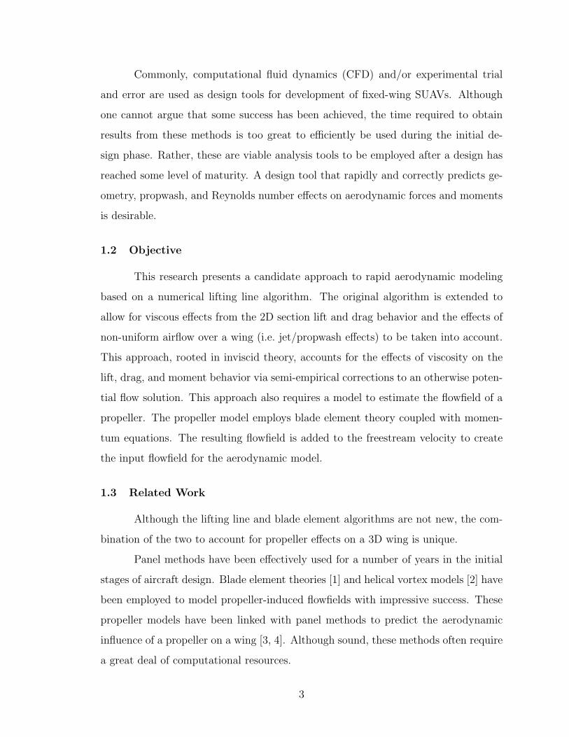
The concept of a tail-sitter VTOL aircraft has been around for over half a
century. The main attraction of such an aircraft is the ability to take o! and land
in a manner similar to a rotorcraft, yet transition to e"cient horizontal flight, thus
achieving higher flight speeds and longer endurance and range. Likely, the most
famous of these aircraft are the Convair XFY-1 Pogo (see Fig. 1.1) and the Lockheed
XFV-1, developed and tested in the 1950’s. These planes quickly proved that the tail-
1
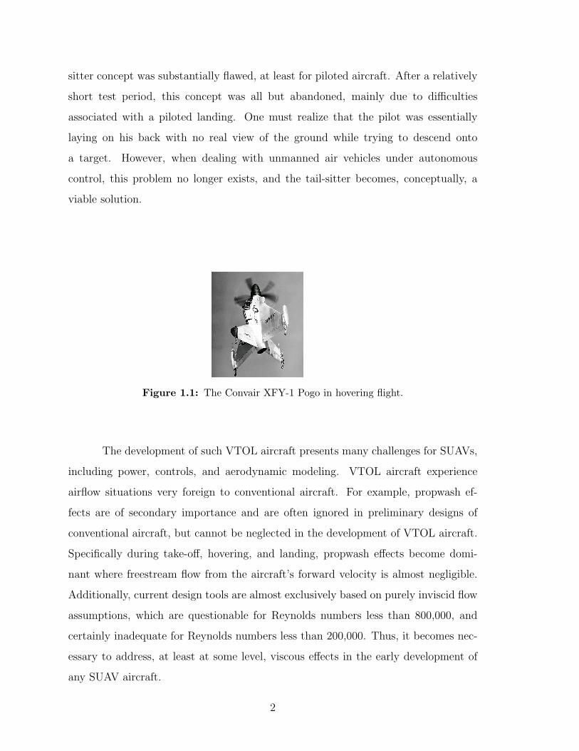
sitter concept was substantially flawed, at least for piloted aircraft. After a relatively
short test period, this concept was all but abandoned, mainly due to di"culties
associated with a piloted landing. One must realize that the pilot was essentially
laying on his back with no real view of the ground while trying to descend onto
a target. However, when dealing with unmanned air vehicles under autonomous
control, this problem no longer exists, and the tail-sitter becomes, conceptually, a
viable solution.
Figure 1.1: The Convair XFY-1 Pogo in hovering flight.
The development of such VTOL aircraft presents many challenges for SUAVs,
including power, controls, and aerodynamic modeling. VTOL aircraft experience
airflow situations very foreign to conventional aircraft. For example, propwash ef-
fects are of secondary importance and are often ignored in preliminary designs of
conventional aircraft, but cannot be neglected in the development of VTOL aircraft.
Specifically during take-o!, hovering, and landing, propwash e!ects become domi-
nant where freestream flow from the aircraft’s forward velocity is almost negligible.
Additionally, current design tools are almost exclusively based on purely inviscid flow
assumptions, which are questionable for Reynolds numbers less than 800,000, and
certainly inadequate for Reynolds numbers less than 200,000. Thus, it becomes nec-
essary to address, at least at some level, viscous e!ects in the early development of
any SUAV aircraft.
2
Commonly, computational fluid dynamics (CFD) and/or experimental trial
and error are used as design tools for development of fixed-wing SUAVs. Although
one cannot argue that some success has been achieved, the time required to obtain
results from these methods is too great to e"ciently be used during the initial de-
sign phase. Rather, these are viable analysis tools to be employed after a design has
reached some level of maturity. A design tool that rapidly and correctly predicts ge-
ometry, propwash, and Reynolds number e!ects on aerodynamic forces and moments
is desirable.
1.2 Objective
This research presents a candidate approach to rapid aerodynamic modeling
based on a numerical lifting line algorithm. The original algorithm is extended to
allow for viscous e!ects from the 2D section lift and drag behavior and the e!ects of
non-uniform airflow over a wing (i.e. jet/propwash e!ects) to be taken into account.
This approach, rooted in inviscid theory, accounts for the e!ects of viscosity on the
lift, drag, and moment behavior via semi-empirical corrections to an otherwise poten-
tial flow solution. This approach also requires a model to estimate the flowfield of a
propeller. The propeller model employs blade element theory coupled with momen-
tum equations. The resulting flowfield is added to the freestream velocity to create
the input flowfield for the aerodynamic model.
1.3 Related Work
Although the lifting line and blade element algorithms are not new, the com-
bination of the two to account for propeller e!ects on a 3D wing is unique.
Panel methods have been e!ectively used for a number of years in the initial
stages of aircraft design. Blade element theories [1] and helical vortex models [2] have
been employed to model propeller-induced flowfields with impressive success. These
propeller models have been linked with panel methods to predict the aerodynamic
influence of a propeller on a wing [3, 4]. Although sound, these methods often require
a great deal of computational resources.
3
An alternative to panel methods has been suggested by Phillips [5] which
extends Prandtl’s lifting line theory to wings with sweep and washout. Phillips showed
that the algorithm matched the accuracy of CFD solutions while requiring only a
fraction of the computational cost. However, this extension of the lifting line theory
has never been used to predict the e!ects of propwash on a wing.
Stone [6] combined a blade element theory with a panel method in the de-
velopment of a tail-sitter UAV. The model was then used to create an aerodynamic
database from which the aerodynamic forces and moments could be found through
interpolation for dynamic simulation. Although the accuracy of the model is not
quantitatively discussed, the model has produced reasonable results which have facil-
itated the development of the UAV. McCormick [7] has also intensely studied VTOL
aerodynamics and presents simplified models for aerodynamic forces and moments
of an aircraft in hover mode. His research is often cited to understand the basic
phenomena of V/STOL flight.
1.4 Contributions
BYU faculty and students have undertaken an e!ort to develop the analysis
tools, control algorithms, and system design of a VTOL SUAV. This research supports
the development of this aircraft and provides a sound aerodynamic modeling package
for students to use in the development of other aircraft for years to come. The
following summarizes the main contributions of the research. This research
• provides a validated aerodynamic modeling package that can be implemented
in the design phases of a VTOL SUAV.
• o!ers alternate solution methods to the equations of the numerical lifting line
algorithm which allows a solution above stall.
• demonstrates the feasibility of the integrated propeller and lifting line models
for analyzing VTOL flight.
• provides an analysis tool available to other students for future aircraft design
projects.
4
1.4.1 Resulting Publications
Hunsaker, D. Snyder, D.O., ”A Lifting-Line Approach to Estimating Propeller
/ Wing Interactions,” 24th Applied Aerodynamics Conference, San Francisco, CA,
June 5-8 2006
Hunsaker, D., ”A Numerical Blade Element Approach to Estimating Propeller
Flowfields,” 45th AIAA Aerospace Sciences Meeting and Exhibit, Reno, Nevada, Jan.
2007 (Accepted)
1.5 Thesis Overview
The numerical model presented in this research can be divided into two sub-
models: 1) an aerodynamic model (lifting line model), and 2) a propeller model (blade
element model). The aerodynamic model is presented first because it is the core of the
computational e!ort of the models. The propeller model is simply a tool to calculate
the flowfield used as the input to the aerodynamic model.
The thesis is divided into four main sections. Chapters 2 and 3 present the
algorithms for the lifting line model and the blade element model respectively along
with relevant assumptions. Chapter 4 presents the validation of each model as well
as the validation of the combined models by comparing the numerical results with
published data. Chapter 5 discusses the integration of the model into a 6 DOF
simulator. Chapter 6 presents the conclusions of the total work.
5

6

Chapter 2
Numerical Lifting Line Model
A numerical method based on Prandtl’s classical lifting line theory is presented
as a low computational cost approach to modeling slipstream e!ects on a finite wing.
This method uses a 3D vortex lifting law along with known 2D airfoil data to predict
the lift distribution across a wing.
2.1 Nomenclature
Ai area of wing section i
ci characteristic chord length for wing section i
ci average chord length at wing section i
CDi section drag coe"cient for wing section i
CLi section lift coe"cient for wing section i
CL!i section lift slope for wing section i
CMi section moment coe"cient for wing section i
d"i directed di!erential vortex length vector at control point i
dFi section aerodynamic force vector for wing section i
dFi magnitude of dFi
f system of equations
F total force on aircraft
[J] Jacobian matrix
M total moment on aircraft
N total number of horseshoe vortices
R residual vector
R magnitude of R
7
ri vector from aircraft CG to control point i
ri1j vector from 1st node on section i to control point on section j
ri2j vector from 2nd node on section i to control point on section j
ri1j magnitude of ri1j
ri2j magnitude of ri2j
Si planform area of wing section i
uai chordwise unit vector at control point i
uni normal unit vector at control point i
usi spanwise unit vector at control point i
ui unit vector in the direction of the local velocity
vij velocity induced at control point j by horseshoe vortex i
Vi velocity vector at control point i
Vi magnitude of Vi
Vai axial component of the velocity at control point i
Vni normal component of the velocity at control point i
Vreli upstream velocity at control point i
Vtoti total velocity at control point i
Vtoti magnitude of Vtoti
!i angle of attack at wing section i
!L0i zero-lift angle of attack for with section i
#i flap deflection for wing section i
#Mi section quarter-chord moment coe"cient at wing section i
#Mvisci viscous correction to the moment coe"cient for wing section i
$i flap e"ciency for wing section i
! vector of vortex strengths
#i vortex strength at control point i
$ relaxation factor
% fluid density
8
2.2 History
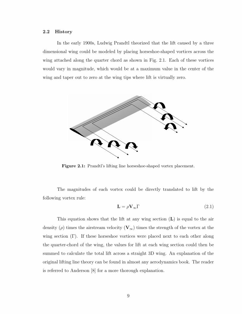
In the early 1900s, Ludwig Prandtl theorized that the lift caused by a three
dimensional wing could be modeled by placing horseshoe-shaped vortices across the
wing attached along the quarter chord as shown in Fig. 2.1. Each of these vortices
would vary in magnitude, which would be at a maximum value in the center of the
wing and taper out to zero at the wing tips where lift is virtually zero.
Figure 2.1: Prandtl’s lifting line horseshoe-shaped vortex placement.
The magnitudes of each vortex could be directly translated to lift by the
following vortex rule:
L = %V!# (2.1)
This equation shows that the lift at any wing section (L) is equal to the air
density (%) times the airstream velocity (V!) times the strength of the vortex at the
wing section (#). If these horseshoe vortices were placed next to each other along
the quarter-chord of the wing, the values for lift at each wing section could then be
summed to calculate the total lift across a straight 3D wing. An explanation of the
original lifting line theory can be found in almost any aerodynamics book. The reader
is referred to Anderson [8] for a more thorough explanation.
9
This method for calculating the forces on a 3D wing has been widely used for
many years due to the simplistic nature of the mathematics. After the development
of the computer, other computational methods became popular and are still avidly
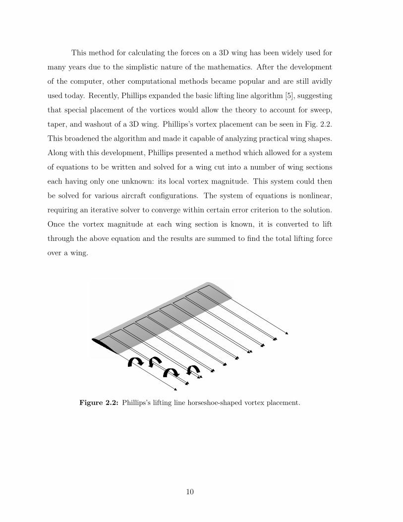
used today. Recently, Phillips expanded the basic lifting line algorithm [5], suggesting
that special placement of the vortices would allow the theory to account for sweep,
taper, and washout of a 3D wing. Phillips’s vortex placement can be seen in Fig. 2.2.
This broadened the algorithm and made it capable of analyzing practical wing shapes.
Along with this development, Phillips presented a method which allowed for a system
of equations to be written and solved for a wing cut into a number of wing sections
each having only one unknown: its local vortex magnitude. This system could then
be solved for various aircraft configurations. The system of equations is nonlinear,
requiring an iterative solver to converge within certain error criterion to the solution.
Once the vortex magnitude at each wing section is known, it is converted to lift
through the above equation and the results are summed to find the total lifting force
over a wing.
Figure 2.2: Phillips’s lifting line horseshoe-shaped vortex placement.
10
2.3 Assumptions
2.3.1 Potential Flow
The original lifting line theory assumes potential flow. Such an assumption is
quite valid at high Reynolds numbers and at low angles of attack. However, at angles
of attack near or above stall, potential flow can no longer be assumed and corrections
must be made. The approach presented here, although rooted in inviscid theory,
accounts for the e!ects of viscosity on lift, drag, and moment via semi-empirical
corrections to an otherwise potential flow solution. The viscous corrections are made
by using 2D viscous data for the section lift and drag behavior. However, no attempt
is made to correct the potential flow e!ects around the tips of wings. This means that
although a wing may be separated from another lifting surface by only an extremely
small distance, the lift at that wing tip could drop to zero. This is not physically
true. In real life, viscous e!ects would prohibit the lift from dropping to zero at small
gaps between wings.
2.3.2 2D Airfoil Characteristics At Each Spanwise Wing Section
The lifting line theory assumes that the lift generated at each spanwise lo-
cation along the wing is equal to that of a 2D airfoil at the same e!ective angle of
attack. (The e!ective angle of attack is the sum of the incident angle of attack to
the freestream velocity and the induced angle of attack resulting from the downwash
caused by the trailing vortices.) This assumption is in order for wings below stall and
lends to very accurate results. It has been shown [9] that flows over wings at high
angles of attack (i.e. above stall) have significant three dimensional properties. More
specifically, at high angles of attack, the flow separates on the upper surface of the
wing and a spanwise vortex forms along the wing. Thus, in order to accurately model
the aerodynamics of a wing above stall, three dimensional e!ects should be taken
into account. Although the lifting line theory assumes nearly two dimensional flow
over each spanwise section of the wing, if post-stall data for the 2D airfoil is known,
the assumption that the lift generated at each spanwise location is equal to that of a
11
2D airfoil at the same angle of attack should still be valid. This approach has been
shown [10] to prove useful as a rough estimate to calculate wing lift above stall.
2.3.3 Elliptical Lift Distribution Initial Guess
High aspect ratio wings below stall have spanwise lift distributions which are
very nearly elliptical in nature. Thus, for wings below stall, it is helpful to start with
an initial elliptical circulation distribution. The formulation of such an initial guess
is discussed in 2.5.1. This initial guess is also applied above stall, although it is not
assumed that the final lift distribution will resemble an elliptical distribution. Thus
it is assumed that an initial guess of an elliptical lift distribution produces reasonable
results below and above stall.
2.4 Formulation
2.4.1 Overview
In the numerical lifting line method presented by Phillips [5], a finite wing is
modeled using a series of horseshoe vortices with one edge bound to the quarter chord
of the wing and the trailing portion aligned with the freestream velocity. A general 3D
vortex lifting law is combined with Prandtl’s hypothesis that each spanwise section
of the wing has a section lift equivalent to that acting on a similar 2D airfoil with the
same local angle of attack.
From the 3D vortex lifting law, the di!erential force vector produced by the
finite wing section i is
dFi = %#iVi " d"i (2.2)
The lift coe"cient of a 2D airfoil can be expressed as an arbitrary function of angle
of attack and flap deflection
CLi = CLi(!i, #i) (2.3)
12
Assuming that this relationship is known at each section, the magnitude of the dif-
ferential force produced by wing section i is
dFi =1
2%V 2
i CLi(!i, #i)Ai (2.4)
Setting the magnitude of Eq. (2.2) equal to the right hand side of Eq. (2.4) for each of
the spanwise sections of the wing produces a system of equations that can be solved
for the vortex strengths at each section. Once all the vortex strengths are known, the
force vector at each section can be computed and summed together to determine the
force and moment vectors acting on the wing. This method has been shown to work
well at predicting the inviscid forces and moments for wings with sweep and dihedral
and aspect ratios greater than four. Accuracy is similar to panel methods or Euler
computational fluid dynamics, but at a fraction of the cost. In addition, systems of
lifting surfaces with arbitrary position and orientation can be analyzed.
2.4.2 Vortex Strengths
Typically, the numerical lifting line algorithm is developed in a nondimensional
form. This is appropriate for conventional aircraft where the freestream velocity is
used as a parameter for nondimensionalization. However, for VTOL flight analysis,
where the freestream velocity can approach zero, a dimensional approach is better
suited.
We begin by setting the magnitude of the force obtained from the section lift
coe"cient at wing section i, Eq. (2.4), equal to the magnitude of the forces determined
from the 3D vortex lifting law, Eq. (2.2). After some rearrangement, we obtain
2#i
!!!!!
"Vreli +
N#
j=1
#jvji
$" d"i
!!!!!# V 2totiAiCLi(!i, #i) = 0 (2.5)
Note that on the LHS, the velocity of section i is split into the local upstream velocity
Vreli and the velocity induced by all horseshoe vortices in the system (initially of
unknown strength). The local upstream velocity di!ers from the global freestream
13
velocity in that it may also have contributions from prop-wash or rotations of the
lifting surface about the aircraft center of gravity. The magnitude of the total velocity
at wing section i is denoted as
Vtoti = |Vtoti| =
!!!!!
"Vreli +
N#
j=1
#jvji
$!!!!! (2.6)
In the above expressions, vji is the normalized velocity induced at section i by
horseshoe vortex j, calculated as
vij =1
4&
%#ij
(ri1j + ri2j)(ri1j " ri2j)
ri1jri2j(ri1jri2j + ri1j · ri2j)
&
+1
4&
%u! " ri2j
ri2j(ri2j # u! · ri2j)# u! " ri1j
ri1j(ri1j # u! · ri1j)
&(2.7)
where #ij is the Kronecker delta (1 if i = j, 0 if i $= j). The local angle of attack at
each section is calculated from the total velocity vector as
!i = tan"1
'
(
)Vreli +
*Nj=1 #jvji
+· uni
)Vreli +
*Nj=1 #jvji
+· uai
,
- (2.8)
Equation (2.5) defines a system of equations that can be solved for the un-
known horseshoe vortex strengths #i. The system can be written in the vector form
f(!) = R (2.9)
where
fi(!) = 2#i
!!!!!
"Vreli +
N#
j=1
#jvji
$" d"i
!!!!!# V 2totiAiCLi(!i, #i) (2.10)
We seek the vector of horseshoe vortex strengths ! that forces the residual
vector R to zero. Notice that Vtoti and ! in Eq. (2.9) are both functions of #. Thus
the system of equations is nonlinear and requires an iterative solver to converge on
the solution.
14
2.4.3 Aerodynamic Forces and Moments
Once the magnitude of #i at each wing section has been found, the forces
resulting from the vortex strengths can be summed to find the overall aerodynamic
force and moment acting on the aircraft. The total force on the aircraft is found by
summing Eq. (2.2) over all wing sections:
F = %N#
i=1
.#i
"Vreli +
N#
j=1
#jvji
$" d"i
/(2.11)
Equation (2.11) provides the total inviscid force vector acting on the aircraft, and
can be divided into the typical lift and induced drag components. A correction for
the viscous drag [11] is added to the model based on the 2D airfoil drag behavior as
a function of angle of attack:
#Fvisc =N#
i=1
1
2%V 2
totiSiCDiui (2.12)
where CDi is the local 2D section drag coe"cient (evaluated at the local angle of
attack).
Similarly, the overall moment vector acting on the aircraft can be found from
M = %N#
i=1
ri ".#i
"Vreli +
N#
j=1
#jvji
$" d"i
/+ #Mi (2.13)
where the first term is the moment due to the aerodynamic forces at each section
acting at a moment arm about the center of gravity, and the second term #Mi is the
2D quarter-chord moment generated by each spanwise segment. #Mi can be easily
obtained by assuming a constant moment coe"cient over each wing section:
#Mi = #1
2%V 2
totiCMi
0 s1
s0
c2 dsusi (2.14)
where usi is the local spanwise unit vector.
15
A viscous correction [11] is also added to the overall moment vector to take
into account the additional moment caused by the viscous drag force at each spanwise
wing section:
#Mvisci =N#
i=1
1
2%V 2
totiSiCDi(ri " ui) (2.15)
2.5 Solvers
The nonlinear system of equations has been solved using various techniques.
Phillips [5] uses a Newton iteration method by calculating the Jacobian of the nondi-
mensionalized system, while Anderson [10] uses a Picard iteration. Below stall the
system displays di!erent characteristics than above stall. A number of solvers were
written in order to facilitate solving the nonlinear equations in both pre- and post-stall
scenarios. Each of these solvers is described below.
2.5.1 Linearized System
In order to achieve the convergence criteria with a small number of iterations,
it is important to obtain a good initial guess for !. To do this, Phillips [5] suggests
finding first a linearized approximation. This system is constructed from the original
system of equations, Eq. (2.10), by dropping all second order terms and assuming a
small induced angle of attack. The full derivation can be found in A.4. This results
in the linear system
2#i
AiCL!i|Vreli " d"i|# V 2
reli
"N#
j=1
#jvji · uni
Vrelj
$
= V 2reli
1tan"1
%Vreli · uni
Vreli · uai
&# !L0i + $i#i
2(2.16)
Once this system is solved for the #is, they can be used as the initial guess for other
solvers.
16
2.5.2 Adjusted Linear Solver
A careful look at the linear solver just described reveals that the resulting
circulation distribution is always elliptical and directly proportional to the lift slope
of the 2D airfoil. At high angles of attack, where the lift slope decreases and deviates
from the initial lift slope of the airfoil, the linear method produces results with sig-
nificant over-predictions for the magnitudes of circulation. However, for most of the
subsequent solvers to converge to a suitable answer, it was found necessary to start
with an initial guess which was much closer to the expected final answer than the
original linearization allowed. Thus it became necessary to find a way to “scale” the
linear solution, especially above stall.
Two options for scaling the solution are presented here.
• Residual Scaling: From each solution, a residual can be calculated using Eq. (2.9)
and Eq. (2.10). Scaling the circulation values by a factor likewise scales the
residual. By applying a Jacobian-type solver to this scenario, the scaling factor
can be found which minimizes the residual of the linear system solution.
• Solution Confidence Scaling: Once a solution has been calculated, one may
note that there are two ways to calculate the resulting forces on the wing. The
most common method is a result of the left half of Eq. (2.5), which is derived
from Eq. (2.2). However, it is often helpful to approach the force calculations
by using the right half of Eq. (2.5), which is derived from Eq. (2.4). Each of
these equations can be used to calculate the total lift on the wing. If these
two values for lift match perfectly, the circulation distribution solution can be
trusted. Further, a significant di!erence between the two lift magnitudes would
suggest that the solution is not sound. A “solution confidence” value can be
calculated by taking the ratio of the smaller calculated lift to the larger. As
this value approaches 1, the solution becomes increasingly valid. Scaling the
circulation values by a factor a!ects the solution confidence value. By applying
a Jacobian-type solver to this scenario, the scaling factor can be found which
produces the solution with the highest solution confidence.
17
Note that the solutions resulting from either scaling method are still elliptical
(for wings without propwash e!ects) and are simply scaled. The tests performed
during this research suggest that the first method, residual scaling, produced the
most valuable initial guesses for the subsequent solvers. This method is implemented
in the resulting computer program. It is worth noting that both methods produced
“better” initial guesses than not scaling the linear solution at all. Additionally, this
scaled linear method has been found to be useful as a final solution estimate above
stall when using another solver causes divergence or requires too much computational
power.
2.5.3 Jacobian Solver
A reliable method for solving the nonlinear system below stall is by using
Newton iterations. Simply stated, the vector of horseshoe vortex strengths ! that
forces the residual vector R to zero of Eq. (2.9) is needed. Starting with an initial
guess for !, we can compute the iterative change from
[J]"! = #R (2.17)
where [J] is the N by N Jacobian matrix:
Jij ='fi
'#j(2.18)
This "! is applied to the previous estimate of ! and iterations are continued until
convergence criterion are met.
Evaluating the partial derivatives of Eq. (2.10), we obtain
Jij = #ij2|Wi| +2Wi · (vji " d"i)
|Wi|#i
# V 2totiAi
'CLi
'!i
Vai(vji · uni)# Vni(vji · uai)
V 2ai + V 2
ni
# 2AiCLi(!i, #i)(Vtot · vji) (2.19)
18
where #ij is the Kronecker delta, and
Wi =
"Vreli +
N#
j=1
#jvji
$" d"i (2.20)
In Eq. (2.19) Vai and Vni are the axial and normal components of the local velocity,
respectively:
Vai =
"Vreli +
N#
j=1
#jvji
$· uai (2.21)
Vni =
"Vreli +
N#
j=1
#jvji
$· uni (2.22)
where uai is the unit vector in the axial (chordwise) direction of section i, and uni
is the unit vector in the normal direction of section i. The complete derivation of
Eq. (2.19) can be found in A.3. When airfoil sections experience angles of attack
beyond stall, the small or negative lift slope of the 2D airfoil data causes divergence
of the Newton iterations. Thus it becomes necessary to explore other solvers.
2.5.4 Picard Solver
A common, simplistic approach to solving the nonlinear system of equations
is through the use of Picard iterations. This solver begins with an initial guess
(calculated from the Best Linear Solver explained above). The initial guess for the
solution vector is used for any imbedded # vector within the system of equations
that makes the system nonlinear. If these imbedded values for # are known, the
system becomes a linear system and can be directly solved using an LU Decomposition
routine. This produces a new solution vector which is theoretically closer to the real
solution than the previous vector. This new guess is then used for the embedded
vectors and the process is repeated until convergence criteria are met.
If #old is known, the linear system can be written as
fi(!) = 2#i
!!!!!
"Vreli +
N#
j=1
#joldvji
$" d"i
!!!!!# V 2totiAiCLi(!i, #i) (2.23)
19
where #old is used to calculate both Vtoti and !. This system can be under-relaxed to
minimize the probability of overstepping the solution.
#inew = $ (#i # #iold) (2.24)
The Picard Solver often requires more iterations to converge than the Jacobian
Solver, but is able to find solutions above stall when the lift slope is negative.
2.5.5 Steepest Descent Solver
The idea behind a Steepest Descent Solver is also simplistic in nature, but
requires a great deal more computational power than the Picard Solver. Starting
from an initial guess, the gradient is found and a line search is performed in that
direction until a local minimum is found. The local minimum is used as the new
initial guess, and the process is repeated until convergence criteria are met.
The purpose of any of the solvers is to minimize the magnitude of the residual
vector R. We will call this magnitude R. We first seek the gradient of R where
R = %R% = %f(!)% (2.25)
This gradient can be found by applying small perturbations to the current solution
and calculating the change in the residual with each perturbation. However, this
is computationally expensive. Thus we seek a computationally e"cient method for
calculating &%f(!)%. By setting
%f(!)% =3
(f(!)2 (2.26)
and
P (!) =1
2
4f1(!)2 + f2(!)2 + . . . + (fN(!)2
5(2.27)
it can be said that
%f(!)% ' P (!) (2.28)
20
Therefore,
&%f(!)% ' &P (!) (2.29)
where
&P (!) =
'
666(
f1"f1
"Γ1+ . . . + fN
"fN
"Γ1
.... . .
...
f1"f1
"ΓN+ . . . + fN
"fN
"ΓN
,
777-(2.30)
and can be rewritten in terms of the Jacobian matrix as
&P (!) = [J]
'
666666(
f1(!)
f2(!)...
fN(!)
,
777777-(2.31)
Therefore, !P (!) can be used as the gradient in the solver because
&P (!) ' &%R% (2.32)
Once the gradient is found, a line search is performed in the direction opposite
of the gradient (the direction of steepest descent) until a local minimum in that
direction is found. This new point is used as the new initial point. The process is
repeated until the solver converges.
Steepest Descent is advantageous in that it is guaranteed to always progress
down-hill and find a local minimum. Additionally, it usually makes good progress dur-
ing the first few iterations. However, if the design space is eccentric, the convergence
process may take a long time.
2.5.6 BFGS Update Solver
The ideal solver would begin by using steepest descent and would gradually
switch to using the Jacobian. This would ensure that good progress would be made
near the beginning of the iterations, and that the optimum would be quickly found
when the iterations near convergence. Such methods exist and are called Rank 1
21
Update methods. These methods choose a direction to search by multiplying the
gradient at the current solution by a direction matrix O as follows
s = #O&f (2.33)
O begins as the identity matrix, and is slowly transformed to the Hessian of the design
space by storing gradients as it traverses the design space. When O is the identity
matrix, the search direction is directly opposite of the gradient at the current solution.
However, as the solver progresses, O becomes the Hessian, and is able to make faster
progress toward the optimum.
Currently, the Broyden-Fletcher-Goldfarb-Shanno (BFGS) Update is consid-
ered to be the best update method. The direction matrix O for this method is found
from
Ok+1 = Ok +
"1 +
4(k
5TOk(k
(%!k)T (k
$"%!k
4%!k
5T
(%!k)T (k
$#
%!k4(k
5TOk + Ok(k
4%!k
5T
(%!k)T ((k)(2.34)
where
(k = &f4!k+1
5#&f
4!k
5, (2.35)
%!k = !k+1 # !k, (2.36)
and k is the iteration number.
2.6 Flaps
In order to predict the aerodynamics of aircraft, the e!ects of control surfaces
on the aircraft must be taken into account. Such e!ects can be accounted for by
altering the lift, drag, and moment coe"cients of wing sections with a deflected
control surface. Equation (2.3) defines the local lift coe"cient, Cli , as an arbitrary
function of both the local angle of attack, !i, and the local flap deflection, #i. The
22
drag and moment coe"cients can also be defined as arbitrary function of the local
angle of attack and flap deflection. This section describes the calculations of each.
2.6.1 Lift Coe#cient
Phillips [11] suggests a simple way to calculate the increase in lift coe"cient
with flap deflection. A brief overview of the method is given here.
Suppose that an airfoil is at an angle of attack, !. If the lift slope, Cl!, of the
airfoil is known, the lift coe"cient can be calculated as an angle multiplied by the lift
slope
Cl = Cl![!# !L0] (2.37)
where !L0 is the zero-lift angle of attack of the 2D airfoil with no flap deflection.
When a positive flap deflection, #f , is added, the camber of the airfoil is increased.
The increase in lift can be approximated by
#Cl = Cl![$f#f ] (2.38)
where $f is the actual flap e!ectiveness and can be defined as follows:
$f = $fi)h)d (2.39)
Here, $fi is the ideal flap e!ectiveness, )h is the hinge e"ciency, and )d is a deflection
e"ciency. The ideal flap e!ectiveness is a function of *f .
$fi = 1# *f # sin *f
&(2.40)
*f is simply a geometric property of the wing and is a function of the ratio of the flap
chord, cf to the section chord, c.
*f = cos"1)2cf
c# 1
+(2.41)
23
The hinge e"ciency, )h, is a function of the ratio of the flap chord to the
section chord. When this ratio is small, the e"ciency is very low. However, as this
ratio approaches 1, the e"ciency approaches 1 in an asymptotic fashion. The hinge
e"ciency can be approximated as
)h = 3.9598 tan"18)cf
c+ .006527
+89.2574 + 4.898015
9# 5.18786 (2.42)
This is a numerical approximation of the graphical relationship presented by Phillips
[11]. The hinge e"ciency should be decreased by 20 percent for unsealed flaps.
The deflection e"ciency, )d, is a function of the deflection. At deflections less
than 10 degrees, the e"ciency can be assumed to be 1. However, above 10 degrees,
the e"ciency begins to drop linearly with deflection angle. The deflection e"ciency
can be approximated from the equation
)d = #.0086 (#) + 1.108 (2.43)
which is also a numerical approximation of the graphical relationship presented by
Phillips [11].
Even with the definitions above, various methods can be used to approximate
the lift coe"cient with varying angle of attack and flap deflection. It is of worth to
be more specific about how the code presented here calculates the lift coe"cient. In
this code, the 2D airfoil data is used as the arbitrary function to calculate the lift
coe"cient with respect to angle of attack with no flap deflection. Additionally, the
lift slope at the local angle of attack with no flap deflection, Cl!,l, is used as the 2D
airfoil lift slope. Thus, a flap deflection at a low angle of attack when the lift slope is
at a maximum is more e!ective than a flap deflection near stall where the lift slope
decreases. Equation (2.37) and Eq. (2.38) combine to produce
Cli = Cli(!i) + Cl!,l[$f#f ] (2.44)
24
2.6.2 Drag Coe#cient
The drag coe"cient can also be approximated by an arbitrary function of the
local angle of attack. Without a flap deflection, the 2D airfoil data is used as the
arbitrary function.
Cdi = Cdi (!i) (2.45)
When a flap deflection exists, the lift coe"cient is first calculated, and the
drag polar is then used as the relation to calculate the drag coe"cient.
Cdi = Cdi (Cli) (2.46)
The drag polar cannot be used when the lift coe"cient caused by the flap deflection
exceeds the maximum lift coe"cient of the 2D airfoil without a flap deflection. In
this case, the e!ect of the flap deflection is ignored, and the drag coe"cient is approx-
imated from the 2D airfoil data at the local angle of attack. Above stall, the flap is
assumed to be totally ine!ective, and the 2D airfoil drag coe"cient is used regardless
of the flap deflection.
2.6.3 Moment Coe#cient
The moment coe"cient is also e!ected by the application of flaps and can be
approximated as an arbitrary function of both local angle of attack, !i, and local flap
deflection, #f .
Cmi = Cmi(!i, #f ) (2.47)
Phillips [11] suggests simply adding a correction factor to the 2D moment coe"cient
at the local angle of attack as follows:
#Cmi = Cm,##f (2.48)
25
Using the ideal moment slope for thin airfoil theory, the change in moment slope with
flap deflection, Cm,#, can be approximated by
Cm,# =sin (2*f )# 2 sin *f
4(2.49)
This value is simply multiplied by the flap deflection and added to the original moment
calculated from the 2D airfoil data at the local angle of attack to find the total section
moment coe"cient.
2.6.4 Flaps Above Stall
Above stall it is assumed that the flaps have no e!ect and can be ignored in
the lift, drag, and moment coe"cient calculations. This can be assumed because the
flow on the upper surface of a wing in stall separates, causing the flaps to lose their
e!ectiveness.
2.7 Summary
A numerical method based on Prandtl’s classical lifting line theory has been
presented. Methods for solving the resulting system of equations have been discussed.
Additionally, the treatment of flap e!ects below and above stall has been addressed.
26
Chapter 3
Numerical Blade-Element Model
A numerical method is presented as a low computational cost approach to
modeling an induced propeller flowfield. This method uses blade element theory cou-
pled with momentum equations to predict the axial and tangential velocities within
the slipstream of the propeller, without the small angle approximation assumption
common to most propeller models.
3.1 Nomenclature
Bd = slipstream development factor
b = number of blades
Cb = batter capacity in mAh
Cl = section coe"cient of lift
cb = blade section chord
Dp = propeller diameter
Eb = battery voltage (Volts)
Em = motor voltage (Volts)
Eo = no load battery voltage (Volts)
Gr = motor gear ratio
Ib = battery current (Amps)
Im = motor current (Amps)
Io = no load motor current (Amps)
J = advance ratio
Kv = motor voltage constant (RPM/volt)
N = number of blade sections
27
Nm = motor RPM
Np = propeller RPM
Pb = motor break power (Watts)
Rb = battery internal resistance (Ohms)
Rc = speed control operating resistance (Ohms)
Rm = motor resistance (Ohms)
Rp = propeller radius
r = radial distance from propeller axis
s = normal distance to propeller plane
Tm = motor torque (Nm)
Tp = propeller torque (Nm)
Vi = blade section total induced velocity
V$i = blade section induced tangential velocity
! = angle of attack to freestream
+t = geometric angle of attack at propeller tip
) = motor and battery system e"ciency
$i = blade section induced angle of attack
$! = blade section advance angle of attack
# = blade section circulation
, = Goldstein’s kappa factor
- = propeller angular velocity
. = throttle setting
* = azimuthal angle of propeller
/b = battery endurance (hrs)
3.2 History
The origins of blade element theory began in the late 1800s and continued
development into the early 1900s. However, lack of the ability to account for the
induced angle of attack which was apparent in experiments hindered the theory’s
28
credibility. Lifting line theory became the credible source for calculating the forces
on both fixed and rotary wings in the early 1900s because of its ability to model the
induced velocity at each wing section. Later, research by Prandtl [12] and Goldstein
[13] allowed for the development of an expression for the circulation about the blade,
and the induced velocity was accounted for in the blade element theory. This theory is
now used mainly for rotary wings as it allows for a fast calculation of the induced axial
and tangential velocities in the plane of a propeller. However, it does not account
for interactions between other fixed or rotary wings. Therefore, it is seldom used for
fixed-wing aircraft analysis.
3.3 Assumptions
The blade element approach, coupled with a slipstream development factor
based on momentum equations, to modeling the propeller flowfield implies a few
underlying assumptions. These are discussed below.
• The axis of the propeller slipstream stays coincident with the axis of the pro-
peller. This can be assumed if the induced axial velocity of the propeller is
much greater than the propeller sideslip velocity.
• There is no mixing between the slipstream and the freestream velocities. No
adjustments are made at the edges of the slipstream to account for mixing with
the freestream. This is obviously a significant assumption, but accounting for
these e!ects is beyond the scope of this initial-stage aerodynamic model.
• The helical trailing vortex sheet maintains a constant pitch.
• Finally, the resultant induced velocities at any distance behind the propeller
are assumed constant with varying azimuthal angle. Therefore, although the
induced velocity downstream from the propeller is a function of * when the
propeller is at an angle of attack, the average velocity at that radius and distance
from the propeller is taken as the induced velocity.
29
3.4 Formulation
In order to predict the time-averaged slipstream behind a propeller, an induced
velocity must be calculated immediately behind the propeller. This velocity is a
function only of the radius if the propeller axis is in line with the freestream velocity
vector, and a function of radius and azimuthal angle, *, if the propeller is not aligned
with the freestream. Phillips [11] presents an approach that does not constrain the
freestream velocity to be aligned with the propeller axis. Thus, o!-axis moments
and forces from the propeller can be found. Dividing the propeller into N discrete
intervals, the induced velocity at each radial blade element can be found by relating
the section circulation to the section induced tangential velocity as shown in Eq. (3.1).
b# = 4&,rV$i (3.1)
Substituting Prandtl’s tip loss factor [12] for Goldstein’s , factor, the following equa-
tion is produced:
bcb
16rCl # cos"1
:
;exp
'
(#b)1# 2r
Dp
+
2 sin +t
,
-
<
= tan $i sin($! + $i) = 0 (3.2)
which can be numerically solved for $i. Once $i is known for a given blade section,
the total induced velocity is found from
Vi =-r sin $i
cos $!(3.3)
This velocity vector is then divided into its axial and tangential components. These
components can be integrated to find the thrust and torque, respectively, of the
propeller.
Once the induced axial and tangential velocities are known at the propeller
plane, the flowfield behind the propeller can be estimated by applying conservation
of momentum equations. The slipstream radius at a distance s behind the propeller
is found by solving for the slipstream development factor suggested by McCormick:
30
[14]
Bd = 1 +s3
s2 + R2d
(3.4)
where Bd is the development factor and approaches 2 as the distance from the pro-
peller plane (s) approaches infinity. Using this radius, and applying conservation of
mass and angular momentum as suggested by Stone [6], the development of the axial
and tangential velocities throughout the slipstream are found.
3.5 Battery and Motor Properties
It is often helpful to predict the behavior of a battery, motor, and propeller
combination. Blade element theory allows the thrust and torque of a propeller to be
predicted. This torque must be matched by the motor to continue operation. Using
a basic electric motor model, the required power of the motor in terms of voltage and
current can be found.
Given the motor, battery, and speed control constants, Kv, Gr, Rm, Io, Rb,
Eo, and Rc, along with the speed control setting, . , and the propeller torque, Tp,
motor and battery variables can be found as follows.
Tm =Tp
Gr(3.5)
Im = .1047KvTm + Io (3.6)
Eb = Eo # ImRb (3.7)
Ib = .Im (3.8)
)s = 1# .078(1# .) (3.9)
Em = )s.Eb # ImRc (3.10)
Nm = Kv (Em # ImRm) (3.11)
Iterations are performed until both the motor RPM and propeller RPM match.
Once these values match, the motor break power, Pb, can be calculated as well as a
31
prediction for the battery endurance, /b.
Pb = .14198TmNm (3.12)
/b =Cb
1000Ib(3.13)
This gives a reasonable prediction for the electrical characteristics of the motor, bat-
tery, and propeller combination.
3.6 Combined Model Assumptions
The numerical lifting line model and the blade element propeller model were
combined to produce a complete algorithm capable of predicting propeller/wing inter-
actions. A major design consideration in the development of the computer code was
the intention of making the algorithm fast enough to link to a real-time simulator. In
order to facilitate this need, a few assumptions within each model were made. These
assumptions are explained in 2.3 and 3.3.
The combination of the two numerical models into a comprehensive model
requires an additional assumption. In order to preserve the low-cost computational
goal of the algorithm, it is assumed that the propeller aerodynamics a!ect the wing,
but the wing aerodynamics do not a!ect the propeller. This allows for the combined
wing and propeller models to first solve the propeller behavior and then solve for the
aerodynamics of the wing in the resultant flowfield. No iterations need be performed
between the flowfields of the wing and propeller, which provides for a faster solution.
32
Chapter 4
Results
4.1 Lifting Line Model
4.1.1 Below Stall
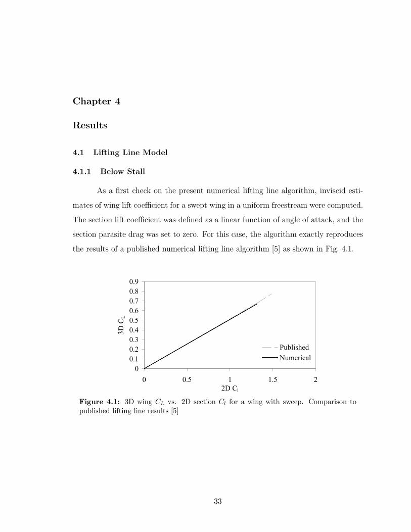
As a first check on the present numerical lifting line algorithm, inviscid esti-
mates of wing lift coe"cient for a swept wing in a uniform freestream were computed.
The section lift coe"cient was defined as a linear function of angle of attack, and the
section parasite drag was set to zero. For this case, the algorithm exactly reproduces
the results of a published numerical lifting line algorithm [5] as shown in Fig. 4.1.
00.10.20.30.40.50.60.70.80.9
0 0.5 1 1.5 22D Cl
3D C
L
PublishedNumerical
0
0.2
0.4
0.6
0.8
1
1.2
1.4
0 20 40 60 80Angle of Attack (degrees)
CL,
Cl
100
2D3D
Figure 4.1: 3D wing CL vs. 2D section Cl for a wing with sweep. Comparison topublished lifting line results [5]
33
4.1.2 Above Stall
Lifting line theory is based on the assumption that at each spanwise section
of the wing, the lift generated by the section circulation can be equated to the lift
generated by a similar 2D airfoil. This works well for angles of attack below stall.
However, above stall this assumption breaks down. Anderson [10] mentions that if
the 2D airfoil data is known above stall, an “engineering solution” may be obtained
using a lifting line algorithm. Additionally, Phillips [11] suggests that his numerical
lifting line method can converge for a wing above stall if the system of equations
is extremely underrelaxed. Others have studied the use of lifting line algorithms
above stall and have made various observations. The results presented in this section
support Anderson’s claim that if the 2D airfoil data is known above stall, a reasonable
estimate for the lift and drag on a 3D wing can be predicted. Additionally, the results
presented here validate the claims of others as will be discussed.
Oscillations
Numerical solutions found for wings near or above stall have been found to have
spanwise oscillations [15, 16] which have discouraged some from trusting these results.
Von Karman is said to have proven that above stall, there are an infinite number of
solutions to the lifting line equation [17]. This includes symmetrical and asymmetrical
solutions. Additionally, the solutions have been shown to be greatly dependent on
the initial guesses for the system [10]. Thus a numerical result of the lift distribution
of a wing above stall should not be accepted as singularly viable.
One attempt to remedy the oscillatory problem was conducted by Mukherjee
[16] who has shown that the algorithm can be “guided” to a more controlled solution
with less oscillation by using a decambering approach. This author also has initial
ideas on how the solution may be guided to a less oscillatory solution. However, it
is beyond the scope of the current research and will not be considered here. Here,
the oscillatory behavior is simply noted and quantified. Further research should be
34
conducted to better understand this behavior and to find methods of damping the
oscillation within the solution.
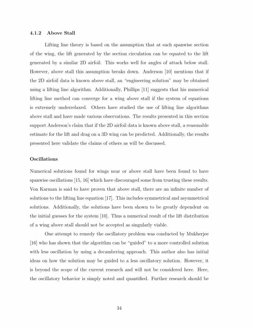
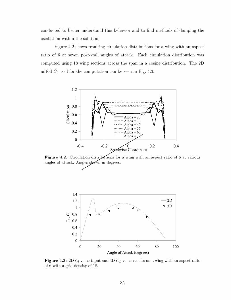
Figure 4.2 shows resulting circulation distributions for a wing with an aspect
ratio of 6 at seven post-stall angles of attack. Each circulation distribution was
computed using 18 wing sections across the span in a cosine distribution. The 2D
airfoil Cl used for the computation can be seen in Fig. 4.3.
0
0.2
0.4
0.6
0.8
1
1.2
-0.4 -0.2 0 0.2 0.4Spanwise Coordinate
Circ
ulat
ion
Alpha = 20Alpha = 30Alpha = 40Alpha = 55Alpha = 60Alpha = 70
0
0.2
0.4
0.6
0.8
1
-0.4 -0.2 0 0.2 0.4Spanwise Coordinate
Circ
ulat
ion
20 Sections60 Sections
Figure 4.2: Circulation distributions for a wing with an aspect ratio of 6 at variousangles of attack. Angles shown in degrees.
00.10.20.30.40.50.60.70.80.9
0 0.5 1 1.5 22D Cl
3D C
L
PublishedNumerical
0
0.2
0.4
0.6
0.8
1
1.2
1.4
0 20 40 60 80Angle of Attack (degrees)
CL,
Cl
100
2D3D
Figure 4.3: 2D Cl vs. ! input and 3D CL vs. ! results on a wing with an aspect ratioof 6 with a grid density of 18.
35
Notice the oscillatory behavior of the circulation distribution above stall. Al-
though the distributions are obviously not correct, the integrated lift across the wing
matches closely to the expected total lift on the wing which can be seen in Fig. 4.3.
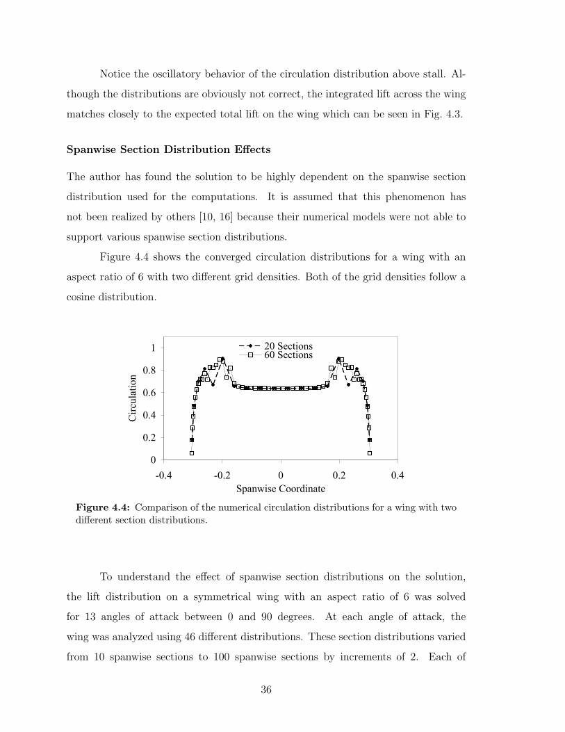
Spanwise Section Distribution E$ects
The author has found the solution to be highly dependent on the spanwise section
distribution used for the computations. It is assumed that this phenomenon has
not been realized by others [10, 16] because their numerical models were not able to
support various spanwise section distributions.
Figure 4.4 shows the converged circulation distributions for a wing with an
aspect ratio of 6 with two di!erent grid densities. Both of the grid densities follow a
cosine distribution.
0
0.2
0.4
0.6
0.8
1
1.2
-0.4 -0.2 0 0.2 0.4Spanwise Coordinate
Circ
ulat
ion
Alpha = 20Alpha = 30Alpha = 40Alpha = 55Alpha = 60Alpha = 70
0
0.2
0.4
0.6
0.8
1
-0.4 -0.2 0 0.2 0.4Spanwise Coordinate
Circ
ulat
ion
20 Sections60 Sections
Figure 4.4: Comparison of the numerical circulation distributions for a wing with twodi!erent section distributions.
To understand the e!ect of spanwise section distributions on the solution,
the lift distribution on a symmetrical wing with an aspect ratio of 6 was solved
for 13 angles of attack between 0 and 90 degrees. At each angle of attack, the
wing was analyzed using 46 di!erent distributions. These section distributions varied
from 10 spanwise sections to 100 spanwise sections by increments of 2. Each of
36
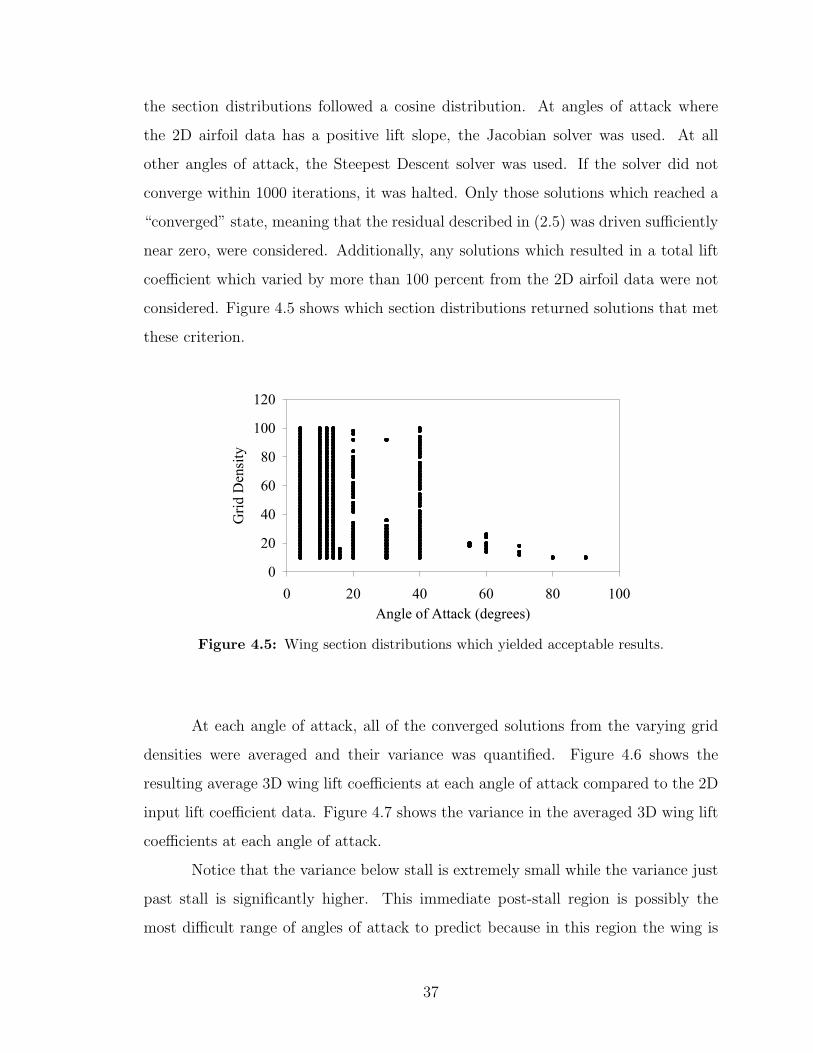
the section distributions followed a cosine distribution. At angles of attack where
the 2D airfoil data has a positive lift slope, the Jacobian solver was used. At all
other angles of attack, the Steepest Descent solver was used. If the solver did not
converge within 1000 iterations, it was halted. Only those solutions which reached a
“converged” state, meaning that the residual described in (2.5) was driven su"ciently
near zero, were considered. Additionally, any solutions which resulted in a total lift
coe"cient which varied by more than 100 percent from the 2D airfoil data were not
considered. Figure 4.5 shows which section distributions returned solutions that met
these criterion.
0
20
40
60
80
100
120
0 20 40 60 80 1Angle of Attack (degrees)
Grid
Den
sity
00
1.0E-081.0E-071.0E-061.0E-051.0E-041.0E-031.0E-021.0E-011.0E+00
0 20 40 60 80 1Angle of Attack (degrees)
CL V
aria
nce
00
Figure 4.5: Wing section distributions which yielded acceptable results.
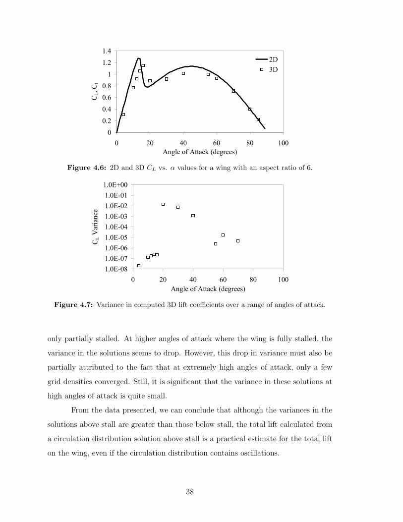
At each angle of attack, all of the converged solutions from the varying grid
densities were averaged and their variance was quantified. Figure 4.6 shows the
resulting average 3D wing lift coe"cients at each angle of attack compared to the 2D
input lift coe"cient data. Figure 4.7 shows the variance in the averaged 3D wing lift
coe"cients at each angle of attack.
Notice that the variance below stall is extremely small while the variance just
past stall is significantly higher. This immediate post-stall region is possibly the
most di"cult range of angles of attack to predict because in this region the wing is
37
00.20.40.60.8
11.21.4
0 20 40 60 80Angle of Attack (degrees)
CL,
Cl
100
2D3D
0
0.5
1
1.5
2
0 20 40 60 80 1Angle of Attack (degrees)
CD
00
2D Exp3D Num
Figure 4.6: 2D and 3D CL vs. ! values for a wing with an aspect ratio of 6.
0
20
40
60
80
100
120
0 20 40 60 80 1Angle of Attack (degrees)
Grid
Den
sity
00
1.0E-081.0E-071.0E-061.0E-051.0E-041.0E-031.0E-021.0E-011.0E+00
0 20 40 60 80 1Angle of Attack (degrees)
CL V
aria
nce
00
Figure 4.7: Variance in computed 3D lift coe"cients over a range of angles of attack.
only partially stalled. At higher angles of attack where the wing is fully stalled, the
variance in the solutions seems to drop. However, this drop in variance must also be
partially attributed to the fact that at extremely high angles of attack, only a few
grid densities converged. Still, it is significant that the variance in these solutions at
high angles of attack is quite small.
From the data presented, we can conclude that although the variances in the
solutions above stall are greater than those below stall, the total lift calculated from
a circulation distribution solution above stall is a practical estimate for the total lift
on the wing, even if the circulation distribution contains oscillations.
38
Lifting Line Limitation
At this point, an insightful realization about the limitations of the lifting line theory
is worthy of note. Namely, that as a finite wing approaches 90# angle of attack, the
lifting line theory is less able to take 3D e!ects into account in the lift, drag, and
moment calculations.
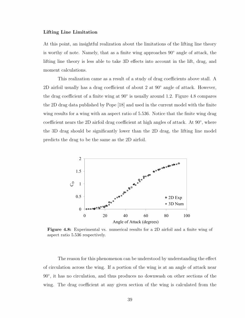
This realization came as a result of a study of drag coe"cients above stall. A
2D airfoil usually has a drag coe"cient of about 2 at 90# angle of attack. However,
the drag coe"cient of a finite wing at 90# is usually around 1.2. Figure 4.8 compares
the 2D drag data published by Pope [18] and used in the current model with the finite
wing results for a wing with an aspect ratio of 5.536. Notice that the finite wing drag
coe"cient nears the 2D airfoil drag coe"cient at high angles of attack. At 90#, where
the 3D drag should be significantly lower than the 2D drag, the lifting line model
predicts the drag to be the same as the 2D airfoil.
00.20.40.60.8
11.21.4
0 20 40 60 80Angle of Attack (degrees)
CL,
Cl
100
2D3D
0
0.5
1
1.5
2
0 20 40 60 80 1Angle of Attack (degrees)
CD
00
2D Exp3D Num
Figure 4.8: Experimental vs. numerical results for a 2D airfoil and a finite wing ofaspect ratio 5.536 respectively.
The reason for this phenomenon can be understood by understanding the e!ect
of circulation across the wing. If a portion of the wing is at an angle of attack near
90#, it has no circulation, and thus produces no downwash on other sections of the
wing. The drag coe"cient at any given section of the wing is calculated from the
39
local angle of attack. Therefore, if there is no downwash, the local angle of attack is
the same as the freestream angle of attack, and the 2D airfoil drag coe"cient is taken
as the section drag coe"cient. This means that as the 3D wing approaches 90# angle
of attack, the 3D drag coe"cient should likewise approach the 2D drag coe"cient
data, which is the case in the numerical results presented in Fig. 4.8.
This phenomenon is the same for lift and moment calculations. Therefore,
as a finite wing nears 90#, its lift, drag, and moment calculations using lifting line
theory approach that of its 2D airfoil. This trend can be seen in Fig. 4.3 and Fig. 4.6.
Notice that as the wing approaches 90# angle of attack, the 3D results increasingly
match the 2D results. This behavior can also be seen in the results presented in the
following section. Similar results were found for moment calculations.
It is important to realize that this characteristic of lifting line theory is a result
of the lift on a wing section (which is directly proportional to the circulation of the
wing section) approaching zero at 90#. Thus, if an airfoil had 2D lift characteristics
that approached zero at 50# rather than at 90#, this phenomenon would occur near
50# rather than at 90#.
4.1.3 NACA 0015 Test Case
To validate the model above stall, numerical results were compared to exper-
imental values published by Critzos [19] and Anderson [10] for a NACA 0015 airfoil.
Critzos published 2D lift, drag, and moment data taken by Pope [18] whose original
publication was not readily available. However, Critzos reports that the data was
taken at a Reynolds number of 1.23 " 106 and that the data was published without
correction factors because the experimentalists found (through some tests and as-
sumptions) that correction factors were not necessary. Anderson published numerical
and experimental lift data for a finite wing with an aspect ratio of 5.563 from 0# to 50#
at a Reynolds number of 2" 106. However, he does not reveal the 2D data used for
his numerical model. Thus Pope’s 2D data was used as input to the current numeri-
cal model and the results were compared to Anderson’s experimental and numerical
results. Figure 4.9 compares the 2D data from Pope and the 3D numerical results
40
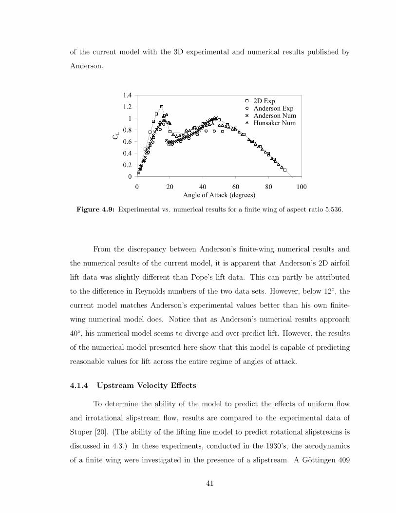
of the current model with the 3D experimental and numerical results published by
Anderson.
0
0.2
0.4
0.6
0.8
1
1.2
1.4
0 20 40 60 80Angle of Attack (degrees)
CL
100
2D ExpAnderson ExpAnderson NumHunsaker Num
Figure 4.9: Experimental vs. numerical results for a finite wing of aspect ratio 5.536.
From the discrepancy between Anderson’s finite-wing numerical results and
the numerical results of the current model, it is apparent that Anderson’s 2D airfoil
lift data was slightly di!erent than Pope’s lift data. This can partly be attributed
to the di!erence in Reynolds numbers of the two data sets. However, below 12#, the
current model matches Anderson’s experimental values better than his own finite-
wing numerical model does. Notice that as Anderson’s numerical results approach
40#, his numerical model seems to diverge and over-predict lift. However, the results
of the numerical model presented here show that this model is capable of predicting
reasonable values for lift across the entire regime of angles of attack.
4.1.4 Upstream Velocity E$ects
To determine the ability of the model to predict the e!ects of uniform flow
and irrotational slipstream flow, results are compared to the experimental data of
Stuper [20]. (The ability of the lifting line model to predict rotational slipstreams is
discussed in 4.3.) In these experiments, conducted in the 1930’s, the aerodynamics
of a finite wing were investigated in the presence of a slipstream. A Gottingen 409
41
airfoil section was employed on a rectangular wing of aspect ratio four (0.8 m span,
0.2 m chord) with circular end caps of diameter 0.32 m. Precautions were taken in the
experimental setup to ensure that the slipstream produced by the 0.12 m diameter jet
was both uniform and non-rotational. The freestream velocity was nominally 30 m/s,
with jet speeds of 35.4 m/s and 40.8 m/s, representing 18% and 36% velocity increases
in the slipstream, respectively.
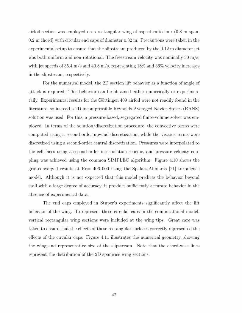
For the numerical model, the 2D section lift behavior as a function of angle of
attack is required. This behavior can be obtained either numerically or experimen-
tally. Experimental results for the Gottingen 409 airfoil were not readily found in the
literature, so instead a 2D incompressible Reynolds-Averaged Navier-Stokes (RANS)
solution was used. For this, a pressure-based, segregated finite-volume solver was em-
ployed. In terms of the solution/discretization procedure, the convective terms were
computed using a second-order upwind discretization, while the viscous terms were
discretized using a second-order central discretization. Pressures were interpolated to
the cell faces using a second-order interpolation scheme, and pressure-velocity cou-
pling was achieved using the common SIMPLEC algorithm. Figure 4.10 shows the
grid-converged results at Re= 406, 000 using the Spalart-Allmaras [21] turbulence
model. Although it is not expected that this model predicts the behavior beyond
stall with a large degree of accuracy, it provides su"ciently accurate behavior in the
absence of experimental data.
The end caps employed in Stuper’s experiments significantly a!ect the lift
behavior of the wing. To represent these circular caps in the computational model,
vertical rectangular wing sections were included at the wing tips. Great care was
taken to ensure that the e!ects of these rectangular surfaces correctly represented the
e!ects of the circular caps. Figure 4.11 illustrates the numerical geometry, showing
the wing and representative size of the slipstream. Note that the chord-wise lines
represent the distribution of the 2D spanwise wing sections.
42
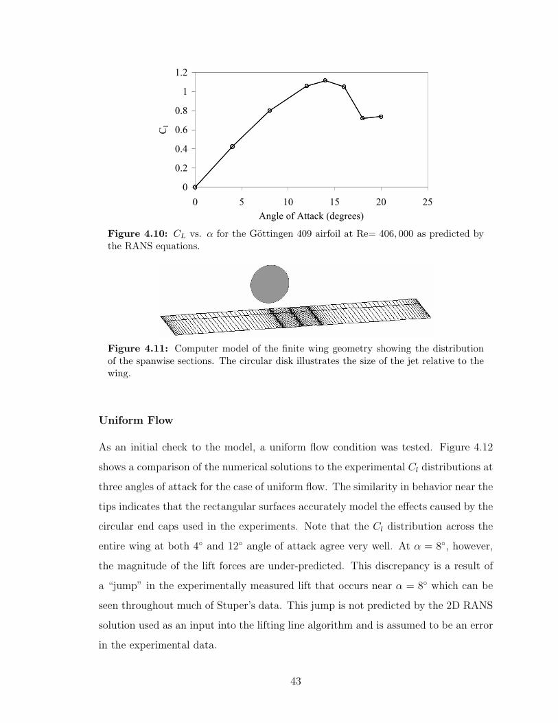
0
0.2
0.4
0.6
0.8
1
1.2
0 5 10 15 20 25Angle of Attack (degrees)
Cl
15
20
25
30
35
40
45
-0.6 -0.4 -0.2 0 0.2 0.4 0.6
Spanwise Coordinate (m)
Vel
ocity
(m/s
)
18%36%
Figure 4.10: CL vs. ! for the Gottingen 409 airfoil at Re= 406, 000 as predicted bythe RANS equations.
Figure 4.11: Computer model of the finite wing geometry showing the distributionof the spanwise sections. The circular disk illustrates the size of the jet relative to thewing.
Uniform Flow
As an initial check to the model, a uniform flow condition was tested. Figure 4.12
shows a comparison of the numerical solutions to the experimental Cl distributions at
three angles of attack for the case of uniform flow. The similarity in behavior near the
tips indicates that the rectangular surfaces accurately model the e!ects caused by the
circular end caps used in the experiments. Note that the Cl distribution across the
entire wing at both 4# and 12# angle of attack agree very well. At ! = 8#, however,
the magnitude of the lift forces are under-predicted. This discrepancy is a result of
a “jump” in the experimentally measured lift that occurs near ! = 8# which can be
seen throughout much of Stuper’s data. This jump is not predicted by the 2D RANS
solution used as an input into the lifting line algorithm and is assumed to be an error
in the experimental data.
43
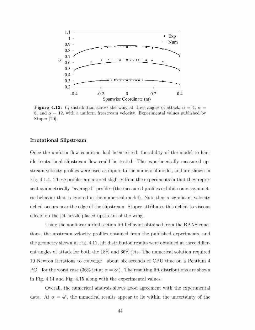
0.20.30.40.50.60.70.80.9
11.1
-0.4 -0.2 0 0.2 0.4Spanwise Coordinate (m)
Cl
ExpNum
0
0.2
0.4
0.6
0.8
1
1.2
-0.4 -0.2 0 0.2 0.4Spanwise Coordinate (m)
Cl
ExpNum
Figure 4.12: Cl distribution across the wing at three angles of attack, ! = 4, ! =8, and ! = 12, with a uniform freestream velocity. Experimental values published byStuper [20].
Irrotational Slipstream
Once the uniform flow condition had been tested, the ability of the model to han-
dle irrotational slipstream flow could be tested. The experimentally measured up-
stream velocity profiles were used as inputs to the numerical model, and are shown in
Fig. 4.1.4. These profiles are altered slightly from the experiments in that they repre-
sent symmetrically “averaged” profiles (the measured profiles exhibit some asymmet-
ric behavior that is ignored in the numerical model). Note that a significant velocity
deficit occurs near the edge of the slipstream. Stuper attributes this deficit to viscous
e!ects on the jet nozzle placed upstream of the wing.
Using the nonlinear airfoil section lift behavior obtained from the RANS equa-
tions, the upstream velocity profiles obtained from the published experiments, and
the geometry shown in Fig. 4.11, lift distribution results were obtained at three di!er-
ent angles of attack for both the 18% and 36% jets. The numerical solution required
19 Newton iterations to converge—about six seconds of CPU time on a Pentium 4
PC—for the worst case (36% jet at ! = 8#). The resulting lift distributions are shown
in Fig. 4.14 and Fig. 4.15 along with the experimental values.
Overall, the numerical analysis shows good agreement with the experimental
data. At ! = 4#, the numerical results appear to lie within the uncertainty of the
44
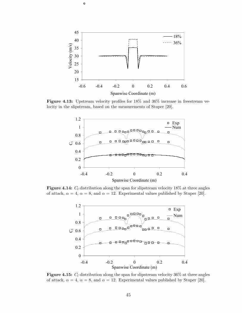
0
0.2
0.4
0.6
0.8
1
1.2
0 5 10 15 20 25Angle of Attack (degrees)
Cl
15
20
25
30
35
40
45
-0.6 -0.4 -0.2 0 0.2 0.4 0.6
Spanwise Coordinate (m)
Vel
ocity
(m/s
)
18%36%
Figure 4.13: Upstream velocity profiles for 18% and 36% increase in freestream ve-locity in the slipstream, based on the measurements of Stuper [20].
0.20.30.40.50.60.70.80.9
11.1
-0.4 -0.2 0 0.2 0.4Spanwise Coordinate (m)
Cl
ExpNum
0
0.2
0.4
0.6
0.8
1
1.2
-0.4 -0.2 0 0.2 0.4Spanwise Coordinate (m)
Cl
ExpNum
Figure 4.14: Cl distribution along the span for slipstream velocity 18% at three anglesof attack, ! = 4, ! = 8, and ! = 12. Experimental values published by Stuper [20].
0
0.2
0.4
0.6
0.8
1
1.2
-0.4 -0.2 0 0.2 0.4Spanwise Coordinate (m)
Cl
ExpNum
0
0.05
0.1
0.15
0.2
0.25
0.3
0 0.5 1 1.5Advance Ratio (J)
Thru
st C
oeff
icie
nt
ExpNum
Figure 4.15: Cl distribution along the span for slipstream velocity 36% at three anglesof attack, ! = 4, ! = 8, and ! = 12. Experimental values published by Stuper [20].
45
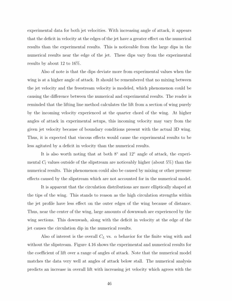
experimental data for both jet velocities. With increasing angle of attack, it appears
that the deficit in velocity at the edges of the jet have a greater e!ect on the numerical
results than the experimental results. This is noticeable from the large dips in the
numerical results near the edge of the jet. These dips vary from the experimental
results by about 12 to 16%.
Also of note is that the dips deviate more from experimental values when the
wing is at a higher angle of attack. It should be remembered that no mixing between
the jet velocity and the freestream velocity is modeled, which phenomenon could be
causing the di!erence between the numerical and experimental results. The reader is
reminded that the lifting line method calculates the lift from a section of wing purely
by the incoming velocity experienced at the quarter chord of the wing. At higher
angles of attack in experimental setups, this incoming velocity may vary from the
given jet velocity because of boundary conditions present with the actual 3D wing.
Thus, it is expected that viscous e!ects would cause the experimental results to be
less agitated by a deficit in velocity than the numerical results.
It is also worth noting that at both 8# and 12# angle of attack, the experi-
mental Cl values outside of the slipstream are noticeably higher (about 5%) than the
numerical results. This phenomenon could also be caused by mixing or other pressure
e!ects caused by the slipstream which are not accounted for in the numerical model.
It is apparent that the circulation distributions are more elliptically shaped at
the tips of the wing. This stands to reason as the high circulation strengths within
the jet profile have less e!ect on the outer edges of the wing because of distance.
Thus, near the center of the wing, large amounts of downwash are experienced by the
wing sections. This downwash, along with the deficit in velocity at the edge of the
jet causes the circulation dip in the numerical results.
Also of interest is the overall CL vs. ! behavior for the finite wing with and
without the slipstream. Figure 4.16 shows the experimental and numerical results for
the coe"cient of lift over a range of angles of attack. Note that the numerical model
matches the data very well at angles of attack below stall. The numerical analysis
predicts an increase in overall lift with increasing jet velocity which agrees with the
46
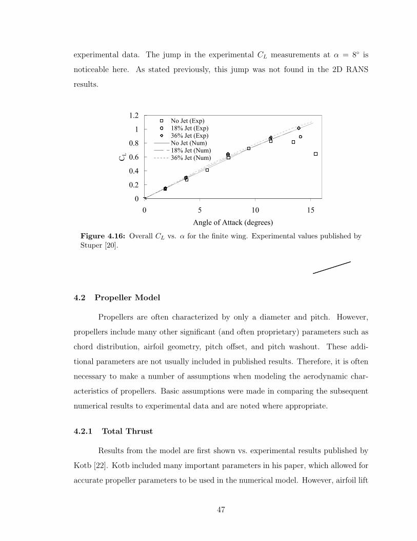
experimental data. The jump in the experimental CL measurements at ! = 8# is
noticeable here. As stated previously, this jump was not found in the 2D RANS
results.
0
0.2
0.4
0.6
0.8
1
1.2
0 5 10 15Angle of Attack (degrees)
CL
No Jet (Exp)18% Jet (Exp)36% Jet (Exp)No Jet (Num)18% Jet (Num)36% Jet (Num)
0
1
2
3
4
5
6
0 1 2 3Freestream Velocity / Static Induced Velocity
Idea
l Pow
er /
Stat
ic P
ower
4
Num. alpha = 0 Num. alpha = 20Num. alpha = 40 Num. alpha = 60Num. alpha = 80 Exp. alpha = 0Exp. alpha = 20 Exp. alpha = 40Exp. alpha = 60 Exp. alpha = 80
Figure 4.16: Overall CL vs. ! for the finite wing. Experimental values published byStuper [20].
4.2 Propeller Model
Propellers are often characterized by only a diameter and pitch. However,
propellers include many other significant (and often proprietary) parameters such as
chord distribution, airfoil geometry, pitch o!set, and pitch washout. These addi-
tional parameters are not usually included in published results. Therefore, it is often
necessary to make a number of assumptions when modeling the aerodynamic char-
acteristics of propellers. Basic assumptions were made in comparing the subsequent
numerical results to experimental data and are noted where appropriate.
4.2.1 Total Thrust
Results from the model are first shown vs. experimental results published by
Kotb [22]. Kotb included many important parameters in his paper, which allowed for
accurate propeller parameters to be used in the numerical model. However, airfoil lift
47
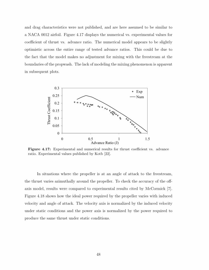
and drag characteristics were not published, and are here assumed to be similar to
a NACA 0012 airfoil. Figure 4.17 displays the numerical vs. experimental values for
coe"cient of thrust vs. advance ratio. The numerical model appears to be slightly
optimistic across the entire range of tested advance ratios. This could be due to
the fact that the model makes no adjustment for mixing with the freestream at the
boundaries of the propwash. The lack of modeling the mixing phenomenon is apparent
in subsequent plots.
0
0.2
0.4
0.6
0.8
1
1.2
-0.4 -0.2 0 0.2 0.4Spanwise Coordinate (m)
Cl
Exp
N
0
0.05
0.1
0.15
0.2
0.25
0.3
0 0.5 1 1.5Advance Ratio (J)
Thru
st C
oeff
icie
nt
ExpNum
Figure 4.17: Experimental and numerical results for thrust coe"cient vs. advanceratio. Experimental values published by Kotb [22].
In situations where the propeller is at an angle of attack to the freestream,
the thrust varies azimuthally around the propeller. To check the accuracy of the o!-
axis model, results were compared to experimental results cited by McCormick [7].
Figure 4.18 shows how the ideal power required by the propeller varies with induced
velocity and angle of attack. The velocity axis is normalized by the induced velocity
under static conditions and the power axis is normalized by the power required to
produce the same thrust under static conditions.
48
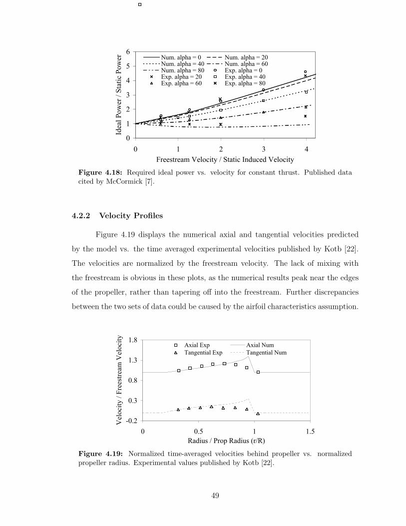
0
0.2
0.4
0.6
0.8
1
1.2
0 5 10 15Angle of Attack (degrees)
CL
No Jet (Exp)18% Jet (Exp)36% Jet (Exp)No Jet (Num)18% Jet (Num)36% Jet (Num)
0
1
2
3
4
5
6
0 1 2 3Freestream Velocity / Static Induced Velocity
Idea
l Pow
er /
Stat
ic P
ower
4
Num. alpha = 0 Num. alpha = 20Num. alpha = 40 Num. alpha = 60Num. alpha = 80 Exp. alpha = 0Exp. alpha = 20 Exp. alpha = 40Exp. alpha = 60 Exp. alpha = 80
Figure 4.18: Required ideal power vs. velocity for constant thrust. Published datacited by McCormick [7].
4.2.2 Velocity Profiles
Figure 4.19 displays the numerical axial and tangential velocities predicted
by the model vs. the time averaged experimental velocities published by Kotb [22].
The velocities are normalized by the freestream velocity. The lack of mixing with
the freestream is obvious in these plots, as the numerical results peak near the edges
of the propeller, rather than tapering o! into the freestream. Further discrepancies
between the two sets of data could be caused by the airfoil characteristics assumption.
-0.2
0.3
0.8
1.3
1.8
0 0.5 1 1.5Radius / Prop Radius (r/R)
Vel
ocity
/ Fr
eest
ream
Vel
ocity
Axial Exp Axial NumTangential Exp Tangential Num
0
0.02
0.04
0.06
0.08
0.1
-0.015 0.035 0.085Axial Distance from Prop Disk (m)
a)
Rad
ial D
ista
nce
from
Pro
p A
xis (
m)
NumericalSlipstream
0
0.02
0.04
0.06
0.08
0.1
0.12
0 0.Axial Distan
Rad
ial D
ista
nce
from
Pro
p A
xis (
m)
Figure 4.19: Normalized time-averaged velocities behind propeller vs. normalizedpropeller radius. Experimental values published by Kotb [22].
49
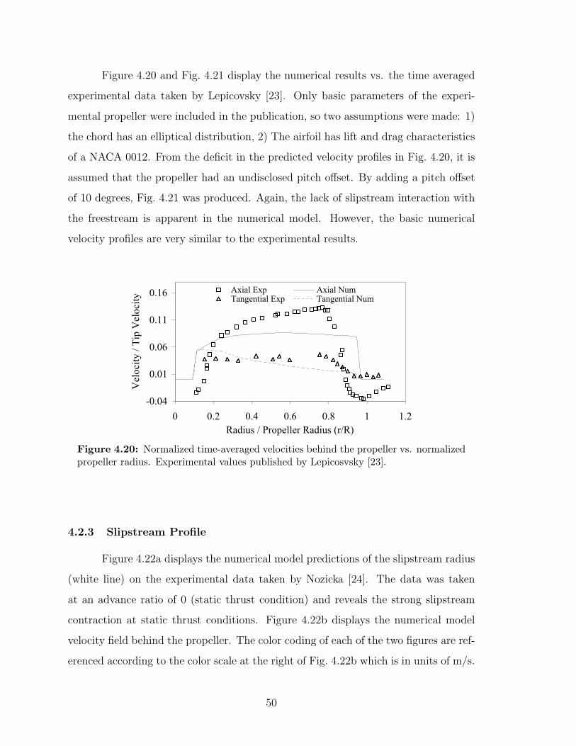
Figure 4.20 and Fig. 4.21 display the numerical results vs. the time averaged
experimental data taken by Lepicovsky [23]. Only basic parameters of the experi-
mental propeller were included in the publication, so two assumptions were made: 1)
the chord has an elliptical distribution, 2) The airfoil has lift and drag characteristics
of a NACA 0012. From the deficit in the predicted velocity profiles in Fig. 4.20, it is
assumed that the propeller had an undisclosed pitch o!set. By adding a pitch o!set
of 10 degrees, Fig. 4.21 was produced. Again, the lack of slipstream interaction with
the freestream is apparent in the numerical model. However, the basic numerical
velocity profiles are very similar to the experimental results.
-0.04
0.01
0.06
0.11
0.16
0 0.2 0.4 0.6 0.8 1 1.2Radius / Propeller Radius (r/R)
Vel
ocity
/ Ti
p V
eloc
ity
Axial Exp Axial NumTangential Exp Tangential Num
Figure 4.20: Normalized time-averaged velocities behind the propeller vs. normalizedpropeller radius. Experimental values published by Lepicosvsky [23].
4.2.3 Slipstream Profile
Figure 4.22a displays the numerical model predictions of the slipstream radius
(white line) on the experimental data taken by Nozicka [24]. The data was taken
at an advance ratio of 0 (static thrust condition) and reveals the strong slipstream
contraction at static thrust conditions. Figure 4.22b displays the numerical model
velocity field behind the propeller. The color coding of each of the two figures are ref-
erenced according to the color scale at the right of Fig. 4.22b which is in units of m/s.
50
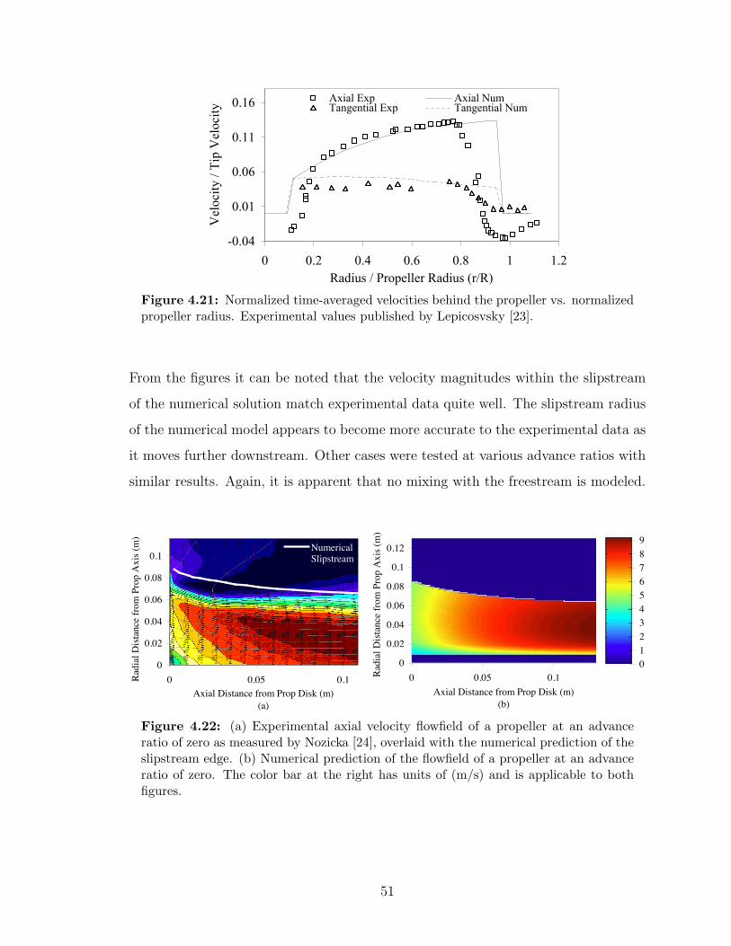
-0.04
0.01
0.06
0.11
0.16
0 0.2 0.4 0.6 0.8 1 1.2Radius / Propeller Radius (r/R)
Vel
ocity
/ Ti
p V
eloc
ity
Axial Exp Axial NumTangential Exp Tangential Num
Figure 4.21: Normalized time-averaged velocities behind the propeller vs. normalizedpropeller radius. Experimental values published by Lepicosvsky [23].
From the figures it can be noted that the velocity magnitudes within the slipstream
of the numerical solution match experimental data quite well. The slipstream radius
of the numerical model appears to become more accurate to the experimental data as
it moves further downstream. Other cases were tested at various advance ratios with
similar results. Again, it is apparent that no mixing with the freestream is modeled.
0
0.02
0.04
0.06
0.08
0.1
0 0.05 0.1Axial Distance from Prop Disk (m)
(a)
Radi
al D
ista
nce
from
Pro
p A
xis (
m)
NumericalSlipstream
0
0.02
0.04
0.06
0.08
0.1
0.12
0 0.05 0.1Axial Distance from Prop Disk (m)
(b)
Radi
al D
ista
nce
from
Pro
p A
xis (
m)
0123456789
Figure 4.22: (a) Experimental axial velocity flowfield of a propeller at an advanceratio of zero as measured by Nozicka [24], overlaid with the numerical prediction of theslipstream edge. (b) Numerical prediction of the flowfield of a propeller at an advanceratio of zero. The color bar at the right has units of (m/s) and is applicable to bothfigures.
51
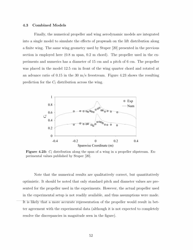
4.3 Combined Models
Finally, the numerical propeller and wing aerodynamic models are integrated
into a single model to simulate the e!ects of propwash on the lift distribution along
a finite wing. The same wing geometry used by Stuper [20] presented in the previous
section is employed here (0.8 m span, 0.2 m chord). The propeller used in the ex-
periments and numerics has a diameter of 15 cm and a pitch of 6 cm. The propeller
was placed in the model 12.5 cm in front of the wing quarter chord and rotated at
an advance ratio of 0.15 in the 30 m/s freestream. Figure 4.23 shows the resulting
prediction for the Cl distribution across the wing.
0.05 0.1xial Distance from Prop Disk (m)
b)
0123456789
0
0.2
0.4
0.6
0.8
1
-0.4 -0.2 0 0.2 0.4Spanwise Coordinate (m)
Cl
ExpNum
Figure 4.23: Cl distribution along the span of a wing in a propeller slipstream. Ex-perimental values published by Stuper [20].
Note that the numerical results are qualitatively correct, but quantitatively
optimistic. It should be noted that only standard pitch and diameter values are pre-
sented for the propeller used in the experiments. However, the actual propeller used
in the experimental setup is not readily available, and thus assumptions were made.
It is likely that a more accurate representation of the propeller would result in bet-
ter agreement with the experimental data (although it is not expected to completely
resolve the discrepancies in magnitude seen in the figure).
52
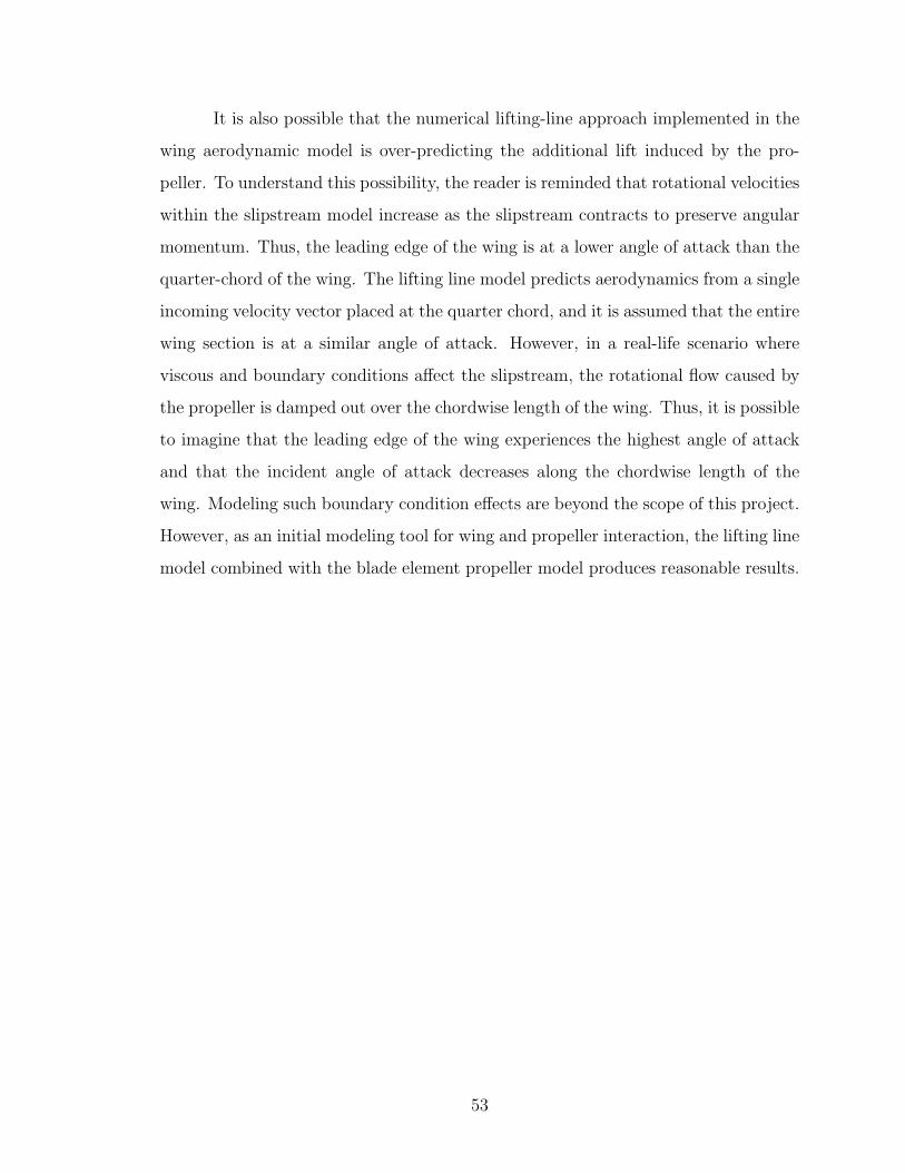
It is also possible that the numerical lifting-line approach implemented in the
wing aerodynamic model is over-predicting the additional lift induced by the pro-
peller. To understand this possibility, the reader is reminded that rotational velocities
within the slipstream model increase as the slipstream contracts to preserve angular
momentum. Thus, the leading edge of the wing is at a lower angle of attack than the
quarter-chord of the wing. The lifting line model predicts aerodynamics from a single
incoming velocity vector placed at the quarter chord, and it is assumed that the entire
wing section is at a similar angle of attack. However, in a real-life scenario where
viscous and boundary conditions a!ect the slipstream, the rotational flow caused by
the propeller is damped out over the chordwise length of the wing. Thus, it is possible
to imagine that the leading edge of the wing experiences the highest angle of attack
and that the incident angle of attack decreases along the chordwise length of the
wing. Modeling such boundary condition e!ects are beyond the scope of this project.
However, as an initial modeling tool for wing and propeller interaction, the lifting line
model combined with the blade element propeller model produces reasonable results.
53

54
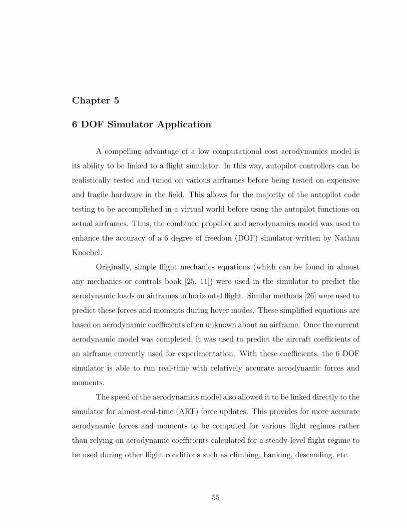
Chapter 5
6 DOF Simulator Application
A compelling advantage of a low computational cost aerodynamics model is
its ability to be linked to a flight simulator. In this way, autopilot controllers can be
realistically tested and tuned on various airframes before being tested on expensive
and fragile hardware in the field. This allows for the majority of the autopilot code
testing to be accomplished in a virtual world before using the autopilot functions on
actual airframes. Thus, the combined propeller and aerodynamics model was used to
enhance the accuracy of a 6 degree of freedom (DOF) simulator written by Nathan
Knoebel.
Originally, simple flight mechanics equations (which can be found in almost
any mechanics or controls book [25, 11]) were used in the simulator to predict the
aerodynamic loads on airframes in horizontal flight. Similar methods [26] were used to
predict these forces and moments during hover modes. These simplified equations are
based on aerodynamic coe"cients often unknown about an airframe. Once the current
aerodynamic model was completed, it was used to predict the aircraft coe"cients of
an airframe currently used for experimentation. With these coe"cients, the 6 DOF
simulator is able to run real-time with relatively accurate aerodynamic forces and
moments.
The speed of the aerodynamics model also allowed it to be linked directly to the
simulator for almost-real-time (ART) force updates. This provides for more accurate
aerodynamic forces and moments to be computed for various flight regimes rather
than relying on aerodynamic coe"cients calculated for a steady-level flight regime to
be used during other flight conditions such as climbing, banking, descending, etc.
55
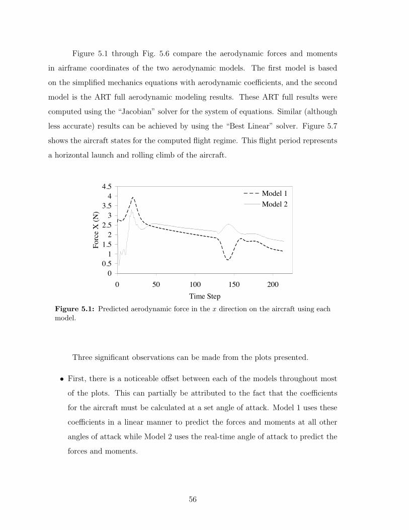
Figure 5.1 through Fig. 5.6 compare the aerodynamic forces and moments
in airframe coordinates of the two aerodynamic models. The first model is based
on the simplified mechanics equations with aerodynamic coe"cients, and the second
model is the ART full aerodynamic modeling results. These ART full results were
computed using the “Jacobian” solver for the system of equations. Similar (although
less accurate) results can be achieved by using the “Best Linear” solver. Figure 5.7
shows the aircraft states for the computed flight regime. This flight period represents
a horizontal launch and rolling climb of the aircraft.
00.5
11.5
22.5
33.5
44.5
0 50 100 150 200Time Step
Forc
e X
(N)
Model 1Model 2
-1.4-1.2
-1-0.8-0.6-0.4-0.2
00.20.40.6
0 50 100 150 200
Time Step
Forc
e Y
(N)
Model 1Model 2
Figure 5.1: Predicted aerodynamic force in the x direction on the aircraft using eachmodel.
Three significant observations can be made from the plots presented.
• First, there is a noticeable o!set between each of the models throughout most
of the plots. This can partially be attributed to the fact that the coe"cients
for the aircraft must be calculated at a set angle of attack. Model 1 uses these
coe"cients in a linear manner to predict the forces and moments at all other
angles of attack while Model 2 uses the real-time angle of attack to predict the
forces and moments.
56
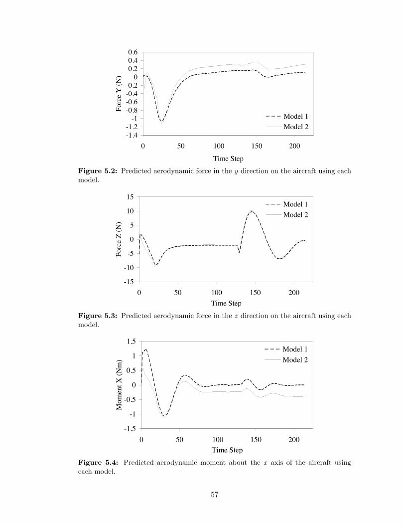
00.5
11.5
22.5
33.5
44.5
0 50 100 150 200Time Step
Forc
e X
(N)
Model 1Model 2
-1.4-1.2
-1-0.8-0.6-0.4-0.2
00.20.40.6
0 50 100 150 200
Time Step
Forc
e Y
(N)
Model 1Model 2
Figure 5.2: Predicted aerodynamic force in the y direction on the aircraft using eachmodel.
-15
-10
-5
0
5
10
15
0 50 100 150 200Time Step
Forc
e Z
(N)
Model 1Model 2
Figure 5.3: Predicted aerodynamic force in the z direction on the aircraft using eachmodel.
-1.5
-1
-0.5
0
0.5
1
1.5
0 50 100 150 200Time Step
Mom
ent X
(Nm
)
Model 1Model 2
-3-2.5
-2-1.5
-1-0.5
00.5
11.5
0 50 100 150 200
Time Step
Mom
ent Y
(Nm
)
Model 1Model 2
Figure 5.4: Predicted aerodynamic moment about the x axis of the aircraft usingeach model.
57
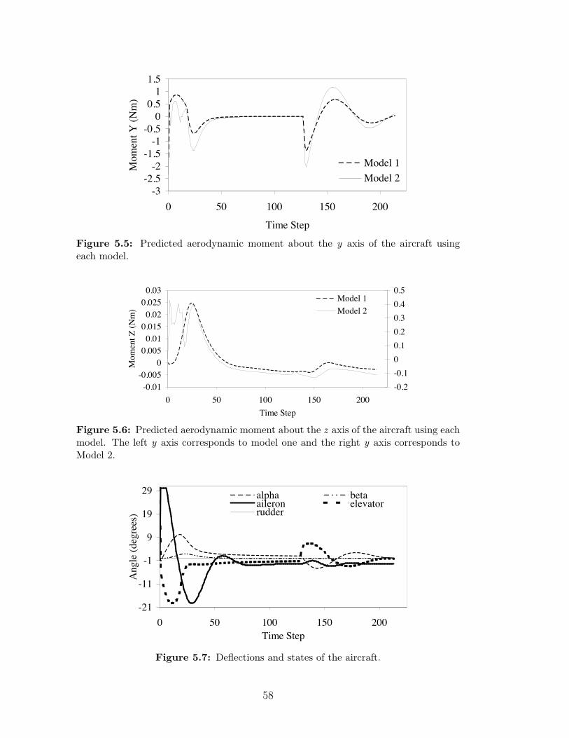
-1.5
-1
-0.5
0
0.5
1
1.5
0 50 100 150 200Time Step
Mom
ent X
(Nm
)
Model 1Model 2
-3-2.5
-2-1.5
-1-0.5
00.5
11.5
0 50 100 150 200
Time Step
Mom
ent Y
(Nm
)
Model 1Model 2
Figure 5.5: Predicted aerodynamic moment about the y axis of the aircraft usingeach model.
-0.01-0.005
00.005
0.010.015
0.020.025
0.03
0 50 100 150 200Time Step
Mom
ent Z
(Nm
)
-0.2-0.100.10.20.30.40.5
Model 1Model 2
Figure 5.6: Predicted aerodynamic moment about the z axis of the aircraft using eachmodel. The left y axis corresponds to model one and the right y axis corresponds toModel 2.
-21
-11
-1
9
19
29
0 50 100 150 200Time Step
Ang
le (d
egre
es)
alpha betaaileron elevatorrudder
Figure 5.7: Deflections and states of the aircraft.
58
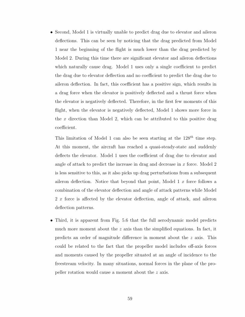
• Second, Model 1 is virtually unable to predict drag due to elevator and aileron
deflections. This can be seen by noticing that the drag predicted from Model
1 near the beginning of the flight is much lower than the drag predicted by
Model 2. During this time there are significant elevator and aileron deflections
which naturally cause drag. Model 1 uses only a single coe"cient to predict
the drag due to elevator deflection and no coe"cient to predict the drag due to
aileron deflection. In fact, this coe"cient has a positive sign, which results in
a drag force when the elevator is positively deflected and a thrust force when
the elevator is negatively deflected. Therefore, in the first few moments of this
flight, when the elevator is negatively deflected, Model 1 shows more force in
the x direction than Model 2, which can be attributed to this positive drag
coe"cient.
This limitation of Model 1 can also be seen starting at the 128th time step.
At this moment, the aircraft has reached a quasi-steady-state and suddenly
deflects the elevator. Model 1 uses the coe"cient of drag due to elevator and
angle of attack to predict the increase in drag and decrease in x force. Model 2
is less sensitive to this, as it also picks up drag perturbations from a subsequent
aileron deflection. Notice that beyond that point, Model 1 x force follows a
combination of the elevator deflection and angle of attack patterns while Model
2 x force is a!ected by the elevator deflection, angle of attack, and aileron
deflection patterns.
• Third, it is apparent from Fig. 5.6 that the full aerodynamic model predicts
much more moment about the z axis than the simplified equations. In fact, it
predicts an order of magnitude di!erence in moment about the z axis. This
could be related to the fact that the propeller model includes o!-axis forces
and moments caused by the propeller situated at an angle of incidence to the
freestream velocity. In many situations, normal forces in the plane of the pro-
peller rotation would cause a moment about the z axis.
59
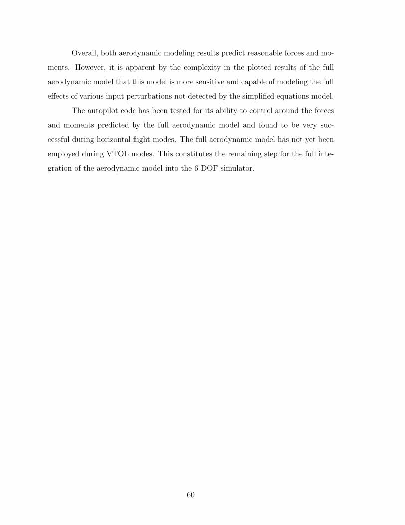
Overall, both aerodynamic modeling results predict reasonable forces and mo-
ments. However, it is apparent by the complexity in the plotted results of the full
aerodynamic model that this model is more sensitive and capable of modeling the full
e!ects of various input perturbations not detected by the simplified equations model.
The autopilot code has been tested for its ability to control around the forces
and moments predicted by the full aerodynamic model and found to be very suc-
cessful during horizontal flight modes. The full aerodynamic model has not yet been
employed during VTOL modes. This constitutes the remaining step for the full inte-
gration of the aerodynamic model into the 6 DOF simulator.
60
Chapter 6
Conclusion
6.1 Lifting Line Model
The lifting line algorithm has proven to be extremely fast and accurate for
3D wings below stall. This provides a very useful tool for the initial design stages
of conventional aircraft. For wings above stall, the lifting line method can be used
with caution. It has shown to produce reasonable values for the integrated lift on a
wing. However, these solutions are often plagued with oscillations in the circulation
distribution, which make the resulting lift, drag, and moment distributions hard to
believe. Further investigation may be able to alleviate these drawbacks to convergence
above stall. Additionally, it has been found that the lifting line theory has significant
limitations in predicting 3D e!ects on a wing near 90# angle of attack. However, the
results produced at high angles of attack are within reason, and can be used with
caution.
6.2 Propeller Model
The accuracy of the propeller model is dependent upon the extent to which the
propeller is correctly characterized within the model. When the propeller is correctly
modeled, the propeller model appears to predict a slightly higher velocity profile
than the experimental data. However, for the initial stages of VTOL aircraft design,
the velocity profiles and slipstream geometry predicted by the model are acceptable.
Thus, a method has been presented and validated which can quickly and accurately
predict propeller slipstream characteristics. The speed of this solution along with its
accuracy will allow the model to be used in preliminary design phases of a VTOL
SUAV.
61

6.3 Combined Models
The results of the combined low-cost models presented above indicate that this
overall approach shows promise for initial aerodynamic design calculations of wings
with significant slipstream e!ects. The lifting line approach to modeling the wing
aerodynamics produces satisfactory results in the presence of a slipstream, often to
within the uncertainty of the experimental measurements. The propeller model also
produces results in good agreement with experimental data. However, the combined
wing and propeller models produce results that, although qualitatively correct, tend
to over-predict the magnitude of the lift perturbations due to the slipstream. This
behavior and its possible remedies should be further investigated.
6.4 Resulting Software: Aither
A software package for aircraft design resulted from the code described above.
The code was written in C++ with a Graphical User Interface developed by Je!
Hogge. The software has proven to be user-friendly and will be implemented by
aircraft design teams at Brigham Young University for future development of both
conventional and VTOL aircraft.
62
Appendix A
Derivation of Lifting-Line Equation
A.1 Nomenclature
Ai area of wing section i
ci characteristic chord length for wing section i
ci average chord length at wing section i
CDi section drag coe"cient for wing section i
CLi section lift coe"cient for wing section i
CL!i section lift slope for wing section i
CMi section moment coe"cient for wing section i
d"i directed di!erential vortex length vector at control point i
f system of equations
F total force on aircraft
[J] Jacobian matrix
M total moment on aircraft
N total number of horseshoe vortices
R residual vector
ri vector from aircraft CG to control point i
ri1j vector from 1st node on section i to control point on section j
ri2j vector from 2nd node on section i to control point on section j
ri1j magnitude of ri1j
ri2j magnitude of ri2j
Si planform area of wing section i
uai chordwise unit vector at control point i
uni normal unit vector at control point i
63
usi spanwise unit vector at control point i
ui unit vector in the direction of the local velocity
vij velocity induced at control point j by horseshoe vortex i
Vreli upstream velocity at control point i
Vtoti total velocity at control point i
Vtoti magnitude of Vtoti
!i angle of attack at wing section i
#i flap deflection for wing section i
#i vortex strength at control point i
% fluid density
A.2 Overview of Numerical Lifting Line Method
In the original numerical lifting line method, a finite wing is modeled using
a series of horseshoe vortices with one edge bound to the quarter chord of the wing
and the trailing portion aligned with the free-stream velocity. A general 3D vortex
lifting law is combined with Prandtl’s hypothesis that each spanwise section of the
wing has a section lift equivalent to that acting on a similar 2D airfoil with the same
local angle of attack.
From the 3D vortex lifting law, the di!erential force vector produced by the
finite wing section i is
dFi = %#iVi " d"i (A.1)
The lift coe"cient of a 2D airfoil can be expressed as an arbitrary function of angle
of attack
Cli = Cli(!i, #i) (A.2)
Assuming that this relationship is known at each section, then the magnitude of the
di!erential force produced by wing section i is
dFi =1
2%V!
2Cli(!i, #i)Ai (A.3)
64
Setting the magnitude of Eq. (A.1) equal to the right hand side of Eq. (A.3)
for each of the spanwise sections of the wing produces a system of equations that can
be solved for the vortex strengths at each section. Once all the vortex strengths are
known, the force vector at each section can be computed and summed together to
determine the inviscid force and moment vectors acting on the wing. This method
has been shown to work well at predicting the inviscid forces and moments for wings
with sweep and dihedral and aspect ratios greater than 4. Accuracy is similar to
panel methods or Euler computational fluid dynamics, but at a fraction of the cost.
In addition, systems of lifting surfaces with arbitrary position and orientation can be
analyzed.
A.3 Jacobian
Phillips [5] derives a nonlinear system of equations which can be solved for
the vortex strengths at each section. This nondimensional approach works well for
conventional aircraft where a freestream velocity can be used to nondimensionalize the
flow. However, for VTOL flight analysis where the freestream velocity can approach
zero, the nondimensional equations do not stand. The following derivation presents a
similar result to Phillips’s nondimensional derivation, but preserves the dimensional
qualities of the flow and aircraft. Such an approach allows not only for freestream
velocities to approach zero, but also for varying velocities across the wingspan.
We begin by setting the magnitude of the force obtained through the lift
coe"cient at wing section i equal to the magnitude of the forces obtained from the #
values.
%#i
!!!!!
"Vreli +
N#
j=1
#jvji
$" d"i
!!!!! =1
2%V 2
totiAiCli(!i, #i) (A.4)
65
where
vij =1
4&
%#ij
(ri1j + ri2j)(ri1j " ri2j)
ri1jri2j(ri1jri2j + ri1j · ri2j)
&
+1
4&
%u! " ri2j
ri2j(ri2j # u! · ri2j)# u! " ri1j
ri1j(ri1j # u! · ri1j)
&(A.5)
Rearranging and canceling % we get
2#i
!!!!!
"Vreli +
N#
j=1
#jvji
$" d"i
!!!!!# V 2totiAiCli(!i, #i) = 0 (A.6)
The system of equations is then written in the vector form
F (!) = R (A.7)
where
Fi(!) = 2#i
!!!!!
"Vreli +
N#
j=1
#jvji
$" d"i
!!!!!# V 2totiAiCli(!i, #i) (A.8)
We want to find the vector of vortex strengths ! that makes the residual vector
R approach zero. Therefore we want the change in the residual vector to be equal
to #R. If we start with an intial guess for the vector !, we can use the Newton
corrector equation and iterate until convergence criteria are met.
[J]"! = #R (A.9)
where [J] is an N by N matrix of partial derivatives.
Jij ='Fi
'#j(A.10)
Eq. A.10 takes on two di!erent forms for two possible cases: Case 1: i $= j
and Case 2: i = j. We will first look at Case 1.
66
Case 1: i $= j : "Fi"Γj
can be divided into two parts (see Eq. (A.8). First, let’s
look at the derivative of the first half of the equation with respect to #j:
'
'#j2#i
!!!!!
"Vreli +
N#
j=1
#jvji
$" d"i
!!!!! (A.11)
This can be rewritten in generic notation as
'
't|f " g| =
f " g
|f " g| ·1
'f
't" g
2
where f is a vector function of t and g is any vector that is not a function of t.
Applying this rule to the equation yields:
'
'#j2#i
!!!!!
"Vreli +
N#
j=1
#jvji
$" d"i
!!!!! =2Wi · (vji " d"i)
|Wi|#i (A.12)
where
Wi =
"Vreli +
N#
j=1
#jvji
$" d"i (A.13)
Now we turn our attention to the derivative of the second half of the equation
with respect to #j:
'
'#jV 2
totiAiCli(!i, #i) (A.14)
where
Vtoti = Vreli +N#
j=1
#jvji (A.15)
Vtoti = |Vtoti| (A.16)
and
!i = tan"1
'
(
)Vreli +
*Nj=1 #jvji
+· uni
)Vreli +
*Nj=1 #jvji
+· uai
,
- (A.17)
67
Here Vtoti and Cli are both functions of #j. The product rule is used for this part of
the equation as follows:
'
'tf(t)g(t) = f $(t)g(t) + f(t)g$(t)
where f(t) and g(t) are both functions of t. Applying this rule to the equation yields:
'Cli'!i
'!i
'#jV 2
totiAi + Cli(!i, #i)Ai'
'#j
4|Vtoti|2
5(A.18)
In order to solve for "!i"Γj
we use the chain rule with the known derivatives of
two basic equations:'
'u
4tan"1 u
5=
1
u2 + 1
'
'u
)v
u
+=
v'u# u'v
v2
Applying the chain rule and the above derivatives we get:
'!i
'#j=
'
6(1
)VniVai
+2
+ 1
,
7-%Vai(vji · uni)# Vni(vji · uai)
V 2ai
&(A.19)
where
Vai =
"Vreli +
N#
j=1
#jvji
$· uai (A.20)
and
Vni =
"Vreli +
N#
j=1
#jvji
$· uni (A.21)
Simplifying yields'!i
'#j=
Vai(vji · uni)# Vni(vji · uai)
V 2ai + V 2
ni
(A.22)
Using rules of vector derivatives we find
'
'#j
4|Vtot|2
5= 2(Vtot · vji) (A.23)
68
Substituting equations A.22 and A.23 into Eq. A.18 and then equations A.12 and
A.18 into Eq. A.10, we get:
Jij ='Fi
'#j=
2Wi · (vji " d"i)
|Wi|#i
# V 2totiAi
'Cli'!i
Vai(vji · uni)# Vni(vji · uai)
V 2ai + V 2
ni
# 2AiCli(!i, #i)(Vtot · vji) (A.24)
Case 2: i = j: Now we turn to Case 2 where i = j. The derivation of Case
2 is identical to Case 1 except that an extra term appears in equation A.12 where
#i = #j which alters the derivative somewhat. Our new answer for Eq. A.12 is:
'
'#j2
!!!!!#i
"Vreli +
N#
j=1
#jvji
$" d"i
!!!!! = 2|Wi| +2Wi · (vji " d"i)
|Wi|#i (A.25)
As a result, we obtain
Jij ='Fi
'#j= 2|Wi| +
2Wi · (vji " d"i)
|Wi|#i
# V 2totiAi
'Cli'!i
Vai(vji · uni)# Vni(vji · uai)
V 2ai + V 2
ni
# 2AiCli(!i, #i)(Vtot · vji) (A.26)
Jij can then be used in Eq. (15) to compute the correction vector %!. Using Newton’s
method, a new ! vector is computed. This process is repeated until the residual
vector, R reaches some convergence criteria.
A.4 Linear Approximation
In order to make the Newton iteration process converge as quickly as possible,
it is important to obtain the best initial guess for the ! vector as possible. To do this,
a linear system of equations can first be solved. This system is constructed from the
original system of equations by dropping all second order terms and using the small
69
angle approximation for the geometric and induced angles of attack. In the original
system,
2#i
!!!!!
"Vreli +
N#
j=1
#jvji
$" d"i
!!!!!# V 2totiAiCli(!i, #i) = 0 (A.27)
!i is defined as
!i = tan"1
'
(
)Vreli +
*Nj=1 #jvji
+· uni
)Vreli +
*Nj=1 #jvji
+· uai
,
- (A.28)
Applying the small angle approximations,
!i =
"Vreli +
N#
j=1
#jvji
$· uni (A.29)
Thus !i can be approximated as the sum of the geometric angle of attack, !geomi ,
and the induced angle of attack, !indi . Thus
!i = !geomi + !indi (A.30)
where
!geomi =Vreli · uni
Vreli
(A.31)
and
!indi =N#
j=1
#jvji · uni
Vrelj
(A.32)
Here Vreli and Vrelj are used to normalize the magnitudes of the dot products . Now
!i can be written as
!i =
1Vreli · uni
Vreli
2+
"N#
j=1
#jvji · uni
Vrelj
$(A.33)
Additionally, we assume that the angle of attack is in the linear lift slope range. Thus,
Cli(!i, #i) = CL!i (!i # !L0i + $i#i) (A.34)
70
By dropping all second order terms (substituting Vreli for Vtoti), the following equa-
tion is produced.
2#i |Vreli " d"i|# V 2reliAiCL!i
.1Vreli · uni
Vreli
2+
"N#
j=1
#jvji · uni
Vrelj
$# !L0i + $i#i
/= 0
(A.35)
A.35 can be rearranged to the linear system
2#i
AiCL!i|Vreli " d"i|# V 2
reli
"N#
j=1
#jvji · uni
Vrelj
$= V 2
reli
%1Vreli · uni
Vreli
2# !L0i + $i#i
&
(A.36)
Once the resulting # vector is solved, it is used as the initial guess in the
nonlinear system.
71

72
Bibliography
[1] P. Lotstedt, “Propeller slip-stream model in subsonic linearized potential flow,”Journal of Aircraft, vol. 29, pp. 1098–1105, 1992. 3
[2] M. Metcalfe, “On the modelling of a fully-relaxed propeller slipstream,”AIAA/SAE/ASME/ASEE 21st Joint Propulsion Conference, 1985. 3
[3] E. S. Levinsky, H. U. Thommen, P. M. Yager, and C. H. Holland, “Lifting-surfacetheory for V/STOL aircraft in transition and cruise. I,” Journal of Aircraft, vol. 6,pp. 488–495, 1969. 3
[4] ——, “Lifting-surface theory for V/STOL aircraft in transition and cruise. II,”Journal of Aircraft, vol. 7, pp. 58–65, 1970. 3
[5] W. Phillips and D. Snyder, “Modern adaptation of Prandtl’s classic lifting-linetheory,” Journal of Aircraft, vol. 37, pp. 662–670, 2000. 4, 10, 12, 16, 33, 65
[6] R. H. Stone, “Aerodynamic modelling of a wing-in-slipstream tail-sitter UAV,”AIAA 2002 Biennial International Powered Lift Conference and Exhibit, 2002.4, 31
[7] B. W. McCormick, Aerodynamics of V/STOL Flight. New York: AcademicPress, 1967. 4, 48, 49
[8] J. D. Anderson, Fundamentals of Aerodynamics, 3rd ed. Avenue of the Americas,New York, NY: McGraw-Hill, 2001. 9
[9] A. W. Winkelmann and J. B. Barlow, “A flowfield model for a rectangular plan-form wing beyond stall,” AIAA Journal, vol. 18, pp. 1006–1008, 1980. 11
[10] J. D. Anderson, S. Corda, and D. M. V. Wie, “Numerical lifting line theory ap-plied to drooped leading-edge wings below and above stall,” Journal of Aircraft,vol. 17, pp. 898–904, 1980. 12, 16, 34, 36, 40
[11] W. F. Phillips, Mechanics of Flight. Hoboken, New Jersey: John Wiley & SonsInc., 2004. 15, 16, 23, 24, 25, 30, 34, 55
[12] L. Prandtl and A. Betz, Vier Abhandlungen zur Hydrodynamik und Aerodynamik,Gottingen, 1927. 29, 30
[13] S. Goldstein, “On the vortex theory of screw propellers,” Royal Society of LondonProceedings Series A, vol. 123, pp. 440–465, April 1929. 29
73
[14] B. W. McCormick, Aerodynamics, Aeronautics, and Flight Mechanics. NewYork: John Wiley & Sons Inc., 1979. 31
[15] E. F. Weener, “Stalled and partially stalled high aspect ratio straight wings,”Ph.D. Dissertation, Dept. of Aerospace Engineering, Univ. of Michigan, 1975.34
[16] R. Mukherjee and A. Gopalarathnam, “Post-stall prediction of multiple-lifting-surface configurations using a decambering approach,” AIAA 2004-0219, 2004.34, 36
[17] W. R. Sears, “Some recent developments in airfoil theory,” Journal of Aeronau-tical Sciences, vol. 23, pp. 490–499, 1956. 34
[18] A. Pope, “The forces and pressures over a NACA 0015 airfoil through 180 degreesangle of attack,” Georgia Tech. Rep., no. E-102, 1947. 39, 40
[19] C. C. Critzos, H. H. Heyson, and R. W. Boswinkel, “Aerodynamic characteristicsof NACA 0012 airfoil section at angles of attack from 0# to 180#,” NACA TN-3361, 1955. 40
[20] J. Stuper, “E!ect of propeller slipstream on wing and tail,” NACA TM 874,1938. 41, 44, 45, 47, 52
[21] P. Spalart and S. Allmaras, “A one-equation turbulence model for aerodynamicflows,” AIAA Paper 92-0439, 1992. 42
[22] M. A. Kotb and J. A. Schetz, “Measurement of three-dimensional turbulent flowbehind a propeller in a shear flow,” AIAA Journal, vol. 24, pp. 570–577, 1986.47, 48, 49
[23] J. Lepicovsky and W. Bell, “Aerodynamic measurements about a rotating pro-peller with a laser velocimeter,” Journal of Aircraft, vol. 21, pp. 264–271, 1984.50, 51
[24] J. Nozieka, J. Novotny, and J. Maticha, “Research on the flow past an aircraftpropeller,” Proceedings of PSFVIP-4, 2003. 50, 51
[25] B. L. Stephens and F. L. Lewis, Aircraft Control and Simulation, 2nd ed. JohnWiley & Sons Inc., 2004. 55
[26] N. B. Knoebel, S. R. Osborne, D. O. Snyder, T. W. McLain, R. W. Beard, andA. M. Eldredge, “Preliminary modeling, control, and trajectory design for minia-ture autonomous tailsitters,” Proceedings of the AIAA Guidance, Navigation,and Control Conference, August 2006 Keystone, Colorado AIAA-2006-6713. 55
74


![]@CFKHCWZHI@physics.gu.se/~tfkhj/MastersThesis/Larsson.pdf · 2007. 5. 22. · fgfgf h ikjAlnm oTlKpLqsrjAltrvuwuyxKo zXpVr{j |KpLq0rvu}xKo|TzXq~lPoT j{r%jAln uXm o!jA LuXmTrvzX 8r](https://img.pdfslide.net/doc/110x75/611eda1c0db25a526b526129/cfkhcwzhi-tfkhjmastersthesislarssonpdf-2007-5-22-fgfgf-h-ikjalnm-otlkplqsrjaltrvuwuyxko.jpg)


![[I] MastersThesis](https://img.pdfslide.net/doc/110x75/563dba07550346aa9aa21670/i-mastersthesis.jpg)