13

Mastery learning of elementary mathematics: Theory and data

1. INTRODUCTION

In this final paper, which is the only one ln this volume that has not been previously published, we develop in some detall a portion of the extensive work we have done together over nearly twenty years on the application of probabilistlc models and methods to problems of curriculum and learning in a computer-based setting. It might seem that there is little connection between this work and what has been described in earlier parts of this volume. In our own mind, however. there is an intimate connection and considerable continuity. The general reason is easy to state. Although much of our work has been motivated by Bayesian considerations and the admiration we have for the pioneering work of Bruno de Finetti in developing concepts of subjective probability, we also recognize how complicated real applications of Bayesian ideas are. Even more generally, we recognize how complicated real applications of normative ideas are. The normative consideratlons that guide the work described here concern how to optimize the course of learning for each mdivldual student. We pick as our example elementary mathematics. partly because there has been such a long history of research on the learning of elementary mathematics, especially arithmetic. throughout this century. beginning at least with the early work of Edward Thorndike, if not even earlier.

As one reflects on the problem of organizing a curriculum for optimizing individual learning, i t is clear that general Bayesian considerations play only a small part. The real problem is to understand as thoroughly as possible the nature of student learning, and, second. to have detailed ideas about what is important for students to learn. The way ln which Bayesian philosophy fits into this program is, on the other hand, clear. I t is characteristic of a Bayesian viewpoint on real-world problems to be skeptical that final solutlons of a smple kind. or ofa kind that can be budt on a bedrock of certainty. are seldom if ever to be found. In this same sense, any claim to have settled all the major questions

149

of student learning or of curriculum organization can only be greeted with proper Bayesian skepticism. What we can hope to do with these two facets of constructing a good computer-based course is to make some headway on understanding better than we do now how they should be organized and on what basis.

We also want to make clear that we do not think, even within a framework of subjective probability, it is possible to reach a definitive normative decision on curriculum organization. Conflict is inevitable and the methods of resolving the conflicts take us beyond Bayesian ideas to game-theoretic ones. In other words, concepts of bargaining, negotiation, and relative positions of power inevitably determine, even if implicitly, how problems of curriculum, especially problems of curriculum emphasis, will be resolved. The normative aspect of the work we have done is conditional in character. Given broad decisions about the nature of the curriculum coverage and the relative distributional emphasis of concepts and skills in that curriculum, we can then apply the methodology developed in this paper to optimize individual student learning. But - and it is important to stress this point - we do not present our work as a straightforward problem of optimization. The many problems of detailed analysis yet to be resolved do not make a direct optimization approach feasible. Much of what we do in this article is the application of specific models of learning that we can then compare with empirical data on student performance. The most elaborate formulation we have yet reached on the interlocking of curriculum organization and mastery criteria is to be found in the final section. Even this rather elaborate model- theoretic formulation is still much too simple in many respects.

In this article we describe extensive work at Stanford University and Com- puter Curriculum Corporation (CCC) over a number of years on computer- assisted instruction in elementary mathematics. Much of what we report here is relevant to other courses, for example, computer-assisted instruction in reading.

The article is organized along the following lines. Section 2 provides a brief review of the main components of mastery learning we have used and analyzed in our work. Section 3 is a detailed treatment of the theory of the learning models we use. Section 4 presents extensive data on how well the models fit some of the main probabilistic features of the students’ responses to exercises in elementary mathematics.

Section 5 turns to the theory of global trajectories of students in a computer- based course. Section 6 then exhibits, mainly in the form of figures and graphs, extensive data on such trajectories in CCC courses on elementary mathematics and reading. Section 7 briefly describes the extension of the work on trajectories to prediction and intervention aimed at helping individual students meet agreed upon achievement goals.

1

150

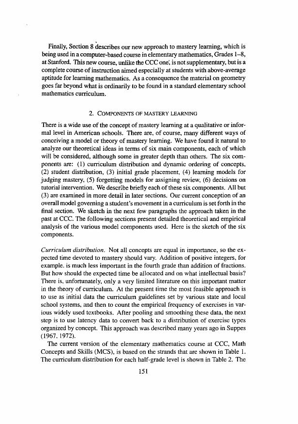
Finally, Section 8 describes our new approach to mastery learning, which is being used in a computer-based course in elementary mathematics, Grades 1-8, at Stanford. This new course, unlike the CCC one; is not supplementary, but is a complete course of instruction aimed especially at students with above-average aptitude for learning mathematics, As a consequence the material on geometry goes far beyond what is ordinarily to be found in a standard elementary school mathematics curriculum,

2. COMPONENTS OF MASTERY LEARNING

There is a wide use of the concept of mastery learning at a qualitative or infor- mal level in American schools. There are, of course, many different ways of conceiving a model or theory of mastery learning. We have found it natural to analyze our theoretical ideas in terms of six main components, each of which will be considered, although some in greater depth than others. The six com- ponents are: (1) curriculum distribution and dynamic ordering of concepts, (2) student distribution, (3) initial grade placement, (4) learning models for judging mastery, (5) forgetting models for assigning review, (6) decisions on tutorial intervention. We describe briefly each of these six components. All but (3) are examined in more detail in later sections. Our current conception of an overall model governing a student’s movement in a curriculum is set forth in the final section. We sketch in the next few paragraphs the approach taken in the past at CCC. The following sections present detailed theoretical and empirical analysis of the various model components used. Here is the sketch of the six components.

Curricrtlrtrn distribution. Not all concepts are equal in importance, so the ex- pected time devoted to mastery should vary. Addition of positive integers, for example, is much less important in the fourth grade than addition of fractions. But how should the expected time be allocated and on what intellectual basis? There is. unfortunately, only a very limited literature on this important matter in the theory of curriculum. At the present time the most feasible approach is to use as initial data the curriculum guidelines set by various state and local school systems, and then to count the empirical frequency of exercises in var- ious widely used textbooks. After pooling and smoothing these data, the next step is to use latency data to convert back to a distribution of exercise types organized by concept. This approach was described many years ago in Suppes (1967, 1972).

The current version of the elementary mathematics course at CCC, Math Concepts and Skills (MCS), is based on the strands that are shown in Table 1 . The curriculum distribution for each half-grade level is shown in Table 2. The

151

Table 1. The strands in Math Concepts and Skills (MCS).

Strand name Strand code Grade levels

Addition AD 0.10-8.90 Applications AP 2.00-8.80 Decimals Dc 3.00-8.90 Division DV 3.50-8.90 Equations EQ 2.00-8.95 Fractions FR 1.10-8.90 Geometry GE 0.03-8.90 Measurement ME O. 10-8.70 Multiplication MU 2.50-8.90 Number concepts NC 0.01-8.90 Probability and statistics PR 7.00-8.90 Problem-solving strategies PS 2.10-6.80 Science applications SA 3.30-7.40 Speed games SG 2.CKM.90 Subtraction su 0.60-8.90 Word problems WP 0.50-8.90

Table 2. Curriculum distribution by half grade of strands in MCS. ~ ~~ ~ ~ _ _ _ _ _ _ _ _ _ ~

Grade Strands levels AD AP DC DV EQ FR GE ME MU NC PR PS SA SG SU WP

0.0 12 O O O O O 4 5 I l O 32 O O O O O O 0.5 9 O O 0 O 0 3 0 1 7 O 3 4 0 0 0 0 3 7 1.0 14 O O O O 6 1 8 18 O 2 9 O O O O 7 8 1.5 17 O O O O 6 1 8 19 O 22 O O O O 11 7 2.0 10 4 O O 4 4 2 0 15 O 9 O 7 O 4 12 8 2.5 14 3 O O 3 3 10 15 2 14 O 7 O 3 14 I l 3.0 13 4 6 0 6 6 6 1 0 6 1 3 0 5 1 6 1 4 4 3.5 1 1 2 6 6 6 6 8 9 1 1 1 1 0 2 . 2 6 1 2 2 4.0 11 3 6 6 6 6 6 7 1 1 1 1 0 5 2 6 1 1 3 4.5 6 2 1 3 6 6 6 6 8 1 2 1 2 0 4 4 6 6 3 5.0 4 7 1 3 4 7 7 1 0 7 9 8 0 4 3 7 6 4 5.5 4 6 1 4 3 7 1 4 1 0 8 7 7 0 3 4 7 3 3 6.0 6 4 1 4 4 7 1 4 7 7 4 7 0 4 4 7 7 4 6.5 8 3 1 5 3 5 1 5 8 8 3 8 0 3 3 7 8 3 7.0 7 4 7 4 3 1 4 7 7 3 7 7 0 7 7 7 4 7.5 8 3 - 8 4 5 1 6 8 8 3 1 0 8 O O 8 8 3 8.0 6 4 7 7 1 3 7 7 7 6 7 9 0 0 7 6 7 8.5 4 4 7 7 1 4 7 7 5 7 7 8 1 1 7 7 7

152

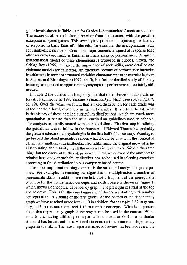
grade levels shown in Table 1 are for Grades 1-8 in standard American schools. The nature of all strands should be clear from their names, with the possible exception of speed games. This strand gives practice in improving the latency of response in basic facts of arithmetic, for example, the multiplication table for single-digit numbers. Continued improvements in speed of response long after no errors are made is familiar in many areas of performance. A simple mathematical model of these phenomena is proposed in Suppes, Groen, and Schlag-Rey (1966), but given the importance of such skills, more detailed and elaborate models are called for. An extensive account of performance latencies in arithmetic in terms of structural variables characterizing each exercise is given in Suppes and Morningstar (1972, ch. 5), but further detailed study of latency learning, as opposed to approximately asymptotic performance, is certainly still needed.

In Table 2 the curriculum frequency distribution is shown in half-grade in- tervals, taken from the 1993 Teacher’s Handbook for Math Concepts and Skills (p. 19). Over the years we found that a fixed distribution for each grade was at too coarse a level, especially in the early grades. It is natural to ask what is the history of these detailed curriculum distributions, which are much more quantitative in nature than the usual curriculum guidelines used in schools. The analysis originally started with such guidelines. The first step in refining the guidelines was to follow in the footsteps of Edward Thorndike, probably the greatest educational psychologist in the first half of this century. Wanting to go beyond the bland generalities about what should be or what is the content of elementary mathematics textbooks, Thorndike made the original move of actu- ally counting and classifying all the exercises in given texts. We did the same thing, but took several further steps as well. First, we converted the numbers to relative frequency or probability distributions, to be used in selecting exercises according to this distribution in our computer-based course.

The most important missing element is the structural analysis of prerequi- sites. For example, in teaching the algorithm of multiplication a number of prerequisite skills in addition are needed. Just a fragment of the prerequisite structure for the mathematics concepts and skills course is shown in Figure 1 , which shows a conceptual dependency graph. The prerequisites start at the top and go down. This is for the very beginning of the course starting with number concepts at the beginning of the first grade. At the bottom of the dependency graph we have reached grade level 1.10 in addition, for example, 1.12 in geom- etry, 1.12 in measurement, and 1.12 in number concepts. What is important about this dependency graph is the way it can be used in the course. When a student is having difficulty on a particular concept or skill in a particular strand, it has turned out to be valuable to construct the minimum dependency graph for that skill. The most important aspect of review has been to review the

153

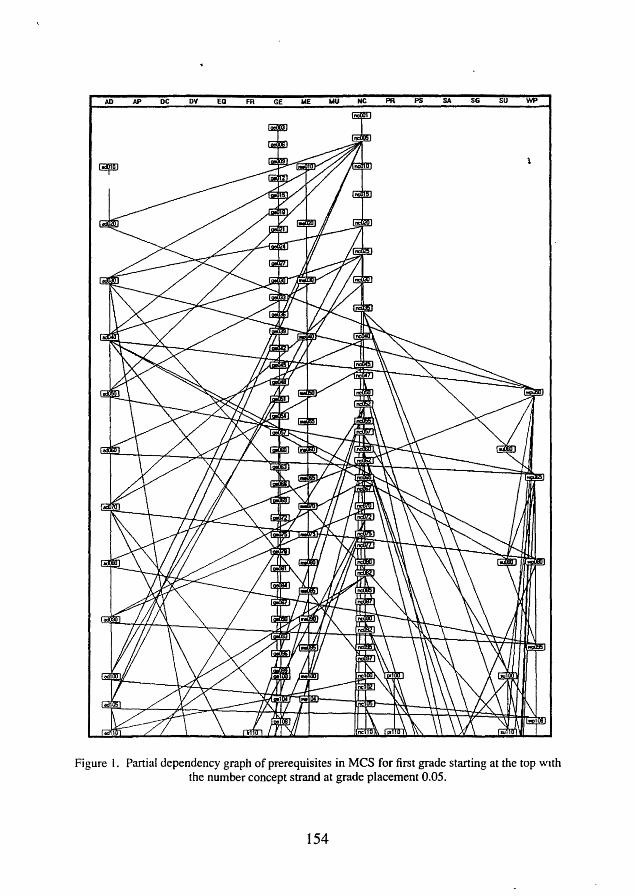
Figure I . Partial dependency graph of prerequisites in MCS for first grade starting at the top with the number concept strand at grade placement 0.05.

154

'

Table 3. Effect ofprerequisite intervention on probability of an error.

Before After

Skill N 1 st Trial 2nd Trial 1st Trial 2nd Trial J

AD 1.80 64 .76 .93 .48 .45 AD 2.15 208 .79 .95 .67 .56 AD 2.95 185 .68 .97 .44 .28 AD 3.80 211 .68 .9 1 .34 .33 DV 4.40 93 .83 .95 .46 .34 DV 5.40 129 .84 .96 -37 .36

prerequisites of a given skill in order to improve performance on it. Rather than simply having review on the skill itself, it turns out, when students are doing badly, it is more efficient to provide review of the prerequisites. In Table 3 we show some data on the reduction in probability of error for students who are having difficulty, after being given intervention by further work on pre- requisites of the given skill. The data shown on the table cover four different levels of addition and two different levels of division, mainly focused on the long-division algorithm. In looking at these data it is important to note that for students who were having real difficulties, the improvements did not reduce their errors to zero but in every case were substantial. Note that what is shown is the probability of an error on two trials before intervention and two trials after intervention on the given skill. h our own judgment the automatic provision for work on prerequisites is one of the most powerful and sophisticated features that can be used in a computer-based course. It is important to emphasize that a prerequisite structure of the kind shown can be important, even when there is not utter clarity and agreement on exactly what the prerequisite structure is, because the psychological analysis, as opposed to the purely mathemati- cal analysis, is less developed and less agreed upon, but has a robustness of its own.

Student distribution. However thorough the curriculum analysis that lies back of the curriculum distribution, individual student differences will necessarily lead to uneven progress for students across the range of concepts and skills in a given curriculum. One student will be much better at executing the standard algorithms of arithmetic than in solving word problems, and another student will be the reverse. So to keep the position of the student at approximately the same level of achievement in all the skills of a basic course in mathematics, a second, individual student distribution is introduced, for purposes of smoothing the actual distribution of grade level achievement across strands - the concepts

155

and skills are organized into homogeneous strands, one for fractions, one for word problems, and so forth.

We outline the basic setup, which depends on selecting two parameters. One is the threshold parameter 8 for how far behind the average grade placement of student s in strand i must be to receive greater emphasis. The second is the parameter a for weighting the curriculum distribution c( i ) , c c( i ) F 1, and assigning weight 1 - a! to the distribution k(i , s) of student s, defined next. Thus, at a given time t the actual distribution d( i , s) used in selecting exercises from strand i for student s is defined as:

(1) d( i , s) = ac(i) + (1 - a ) k ( i , s),

with O 6 a! 6 1. To define k( i , s), let

ii(s) - g ( i , s) if ã(s) 2 g ( i , s) + 8, h(i, s) =

otherwise,

where g(i, s) is, at the time t , the grade level achievement in strand i of student s, and ã(s) is the weighted average grade level achievement of s at time t with the averaging being across strands weighted by the curriculum distribution c ( i ) . Finally,

The qualitative analogue of equation (1) is used by any observant intelligent human tutor. In this instance it is easy to implement something that probably does a better job in most cases.

Initial placement motion (IPM). The purpose of IPM is to move a student rapidly up or down in grade placement on the basis of performance in an initial sequence of sessions. The objective is to find the appropriate grade placement for the student to begin the course,

We begin with some preliminaries. Let G,,n 2 O, denote the student’s average grade level at the end of session n, achieved under the standard curriculum motion, Go being the initial (entering) grade level. Then A,, = G, - G,,-, , n >, 1, is the grade level increment (positive or zero) achieved during session n under the standard curriculum motion.

Let Y,, n 3 1, be the grade level increment (positive or negative) achieved at the end of session n under the IPM motion, which is defined explicitly later.

156

If Zn , n b 1, denotis the grade level at the end of IPM session n, we can write: n n

Z, = G ~ + C A ¿ +):yi . i= l r=l *

This means that the stochastic process {Z,,; n 3 l}, the grade level at the end of IPM session n, is the sum of the following processes:

(i) {An; n 2 l}, the curriculum process which is defined by the parameters of

(ii) {Yo; n 3 l}, the IPM process, defined as follows: the standard curriculum motion

( O otherwise,

with al, a2, ß l , 8 2 positive real numbers, Y 1 l . . . l Y,, independent random variables, (TCOR), the total number of correct exercise in session i, and (TATT), the total number of attempted exercises in session i. In order to complete the definition of the IPM process, the probability distribution of the random variables Y 1 , . . . , Y,, must be given. These mathematical developments are not considered here.

Learning models of mastery. Our problem is to decide when performance on a given class of essentially equivalent exercises satisfies some criterion. In many situations it is assumed that the underlying process that is being sampled is sta- tionary - at least in the mean. The first simple model we shall consider is of this type. A more realistic assumption in dealing with student behavior is that learn- ing is occurring - both individually and in the mean - so that the process is not stationary. The second model is of this type. The third model is explained later.

Components ( 5 ) and (6) on forgetting models and tutorial intervention are discussed later.

3. LEARNING MODELS: THEORY

Although in the intended applications the number of possible student responses is usually large - and therefore the probability of guessing a correct answer is close to zero - we shall consider here only correct and incorrect responses. With this restriction:

A O , ~ = event of incorrect response on trial n , A 1 .,, = event of correct response on trial n l

157

x,, = possible sequence of correct and incorrect responses firom triai I to n

Qn = P( Ao, a = mean probability of an error on trial n, inclusive,

%.n = P(Ao* l &-l), (I 41 = P(A0.1).

Also, AoSn and AI,^ are the corresponding random variables. We shall alsq use X, = as our most important random variable.

For simplicity we shall assurne a fixed initial probability q = P ( Ao. 1 ) rather than a prior distribution on the unit interval for this probability. Given the extensive knowledge of this distribution, assuming that all the weight is on q is not unrealistic.

In Model I the assumptions are:

We can easily prove the significant fact of stationarity of the mean probability P ( A 0 . n ) .

THEOREM 1 l n Model l , for all n, P(AoJ = 91.

P roof.

We have at once then

In Model II we generalize Model I to unequal os on the assumption that learning is occwing during the trials, so we assume 01 < w, and we replace (i) and (ii) by (i’) and (ii’):

To express results compactly, we define moments:

(6) Vi,n = C P ’ ( A ~ , ~ I xn-1)P(xn-l)- X

THEOREM 2 In Model I I ,

Proof. By the same methods used for Theorem 1,

In the case of both Models I and II the asymptotic behavior is well known (Karlin, 1953). All sample paths converge to O or 1, with the exact distribution depending on the initial distribution, and in the case of Model II, the relative values of w1 and w. Of course, in the case of Model II, detailed computations are difficult. With the asymptotic dependence on initial conditions, neither process is ergodic.

Here is how either model would work computationally in practice. A student is exited upward from a class when < q*, where q: is the nonnative the- shold. for example, we might set q* = .15, corresponding to a probability cor- rect of -85. Notice that both models are noncommutative, and thus give greater weight to later responses. These models are derived from learning models that have been extensively studied. For pedagogical purposes in a computer environment they are computationally simple. The history of a sequence - O01 l001 1 1, for example - is absorbed in the current qx,n, and no other data need be kept, except possibly a count of the number of exercises.

Still more suitable is a third model that has both a parameter for individual paths, such as in Model I, or possibly two such parameters as in Model II, together with a uniform learning parameter a! that acts constantly on each trial, since the student is always told the correct answer. For simplicity we shall

159

consider the two-parameter model using a and w, which are assumed to lie in the open interval (O, 1).

In Model III the assumptions are:

(iv) P(Ao,n+t I Ao.nxn-1) = (1 -w)aP(Ao.n I xn-1) +au, (v) P(Ao,n+r I Al,nXn-l) = (1 - wW(Ao.f f I xn-l).

It is then easy to prove by the methods already used, or equivalently in terms of the random variable Xn, the following:

(8) E(X,+I 1 Xn, . - . X,) = k E ( X , I L - 1 , - - . 9 XI) +cuwX,, with k = a( l - w) .

PROPOSITION Let (X,, n 3 1 } he a learning process of Qpe III . Then for each n 3 1 Ilve have:

n

(9) E(x ,+~ I X,,. . . X , ) P E ( X I ) + a u x X i P - ' . ' = l

where E (XI ) = P (X , = l ) = q ìs the initial condition of the process.

Thus. trial t1 + 1 of the process with initial condition E ( X 1 ) = q can be viewed as the second trial of the same process with the observed value of €(X, I X,-,. . . . . X I ) as initial condition. It is also clear from (9) that for each n >, 1, the conditional expectation of X,+! given xi. i = 1. . . . . n. is a random linear function of X, with coefficients auk"-'.

We also hase the recursion:

( l 1 ) E ( X , + I ) = aE(X , ) .

Then

E(X,+I) = EWX,+I I x,. * - - * X I ) ) = a( 1 - w ) E ( X , ) + crwE(X,) = a ! E ( X , ) .

It follows at once from ( 1 1 ) that the mean learning curve is given by:

(12) E ( X , , + , ) = a " E ( X 1 ) .

160

Similarly,

l (13) VAR(X,) = E(X,)(l - E(X,)).

And we can then prove from (12) and ( 13): i.

(14) VAR(Xn+1) dE(X1)(1 - a"E(X1)).

We next consider the covariance recursion.

(15) E(X,+,+,X,) = aE(X,+,X,).

Proof.

Then, taking expectation we have

By similar methods, we can easily show:

The expected number of errors in n trials is:

In fact:

with

(19)

161

Furthermore,

1=1

Learning following errors. We now prove some results about learning after er- rors are made. That learning is different after incorrect responses in comparison with correct responses is one of the most significant features of Model III.

PROPOSITION For each n 2 1, E(Xn+I I Xn, . . . , X I ) M={q, f i } .

Proof

PROPOSITION Let 4 < au/( 1 - k ) . Then for each n 3 l we have:

E(X, 1 X , - I . . . . , X I ) iff X, = O.

written in the equlvalent form: Q!w x+,, ..., X , ) - X n

1 - k

The concluslon follows from the preceding proposition. These two propositions show that with 4 a o / ( l - k ) and for each n 3 1, E(Xn+I I X,, . . . . X I ) decreases if X,, = O and increases if X, = 1. Thus. learning following errors will not occur. With q > a o / ( l - k), let q* = q - [aw/(l - k ) ] . Then we can write:

n

~ ( ~ n - 1 I X,. . . . . X , ) = krlq* + k"- + kn-'Xi . ( ,""x / = l ) Following errors only we have:

au E(X,+I I x, = l , i = 1 . . . . . n ) = k"q* + -

1 - k ' Thus, learning following errors only will occur if and only if q > au/( 1 - k ) and its magnitude will be at most 4*. In general. for each n 3 1 the realizations

162

Figure 2. The graph shows the Model III learning curves for a sequence of errors only; the two cases depend on whether the inihd q is less than or greater than y.

of E(X,+1 I Xn, . . . , X,) satisfy the inequality

1 -k" k"q 6 E(Xn+l I Xn, - a , X I ) < knq + QIU- l - k '

Figure 2 shows the importance of the bound y = QU/ (1 - k).

Sequential analysis. We now turn to joint probabilities such as P(X1 = xi, X2 = x?, X3 = x3, X4 = x4), where x, = O or 1. First,

P(Xi+ l = 1 I XI, . * . , X,) = K P ( X , = 1 I x,, . . , Xl-l) + aox,.

In MCS the following rnastery-stopping rule was used for moving to the next concept in a strand, with different parameter values set for different concepts. ln fact. the concepts were, for this purpose, put in one of six classes. We shall not go into the details of parameter selection for these six classes.

DEFINITION A mastery-stopping rule adapted to the process {X,, n 3 l} with threshold t = k m q , m 3 l , is a random index of the form:

inf{n : E(X,+l I XI, . . . , X,) < k m q } vthis set is (21) N(m) = nonempty.

otherwise.

163

We will say that th<mastery level following the stopping rule N (m) is (1 - P g ) . In other words, with this mastery level the probability correct on trial N ( m ) is equal to or greater than 1 - kmq.

4. LEARNING MODELS: DATA

Data analysis of mean learning curves and sequences of responses. Figures 3-6 show four mean learning curves for third and fourth grade exercises in addition, multiplication, and division of whole numbers and addition of fractions. The grade placement of each class of exercises is shown in the figure caption, for example, 3.55 for multiplication. But this does not mean that all the students doing these exercises were in the third grade, for, with the individualization possible, students can be from several different chronological grade levels. The sample sizes on which the mean curves are based are all large, ranging from 6 1 1 to 1,283 students. The students do not come from one school and certainly are not in any well-defined experimental condition. On the other hand, all of the students were working in a computer laboratory in an elementary school run by a proctor. so there was supervision of a general sort of the work by the students, especially in terms of schedule and general attention to task. For each

"'T

Y "

I 3 5 7 9 I l 13 I5 17 19 21 23 25 27 29 31 33 35 37 39

Flgure 3. Mean leamtng curve for addltion strand of MCS at grade level 3.10. the sample uze IS

6 1 1 students. y = 0.269. (Y = 0.840, standard error of estlmate (s.e.e.) = 0.0059. mean absolute devlatton (mad.) = 0.0041. max. dev. = 0.0209.

164

Figure 4. Mean leammg curve for subtraction strand of MCS at grade level 4.10; the sample size is 719 students, q = 0.394, a! = 0.854, s.e.e. = 0.0062. m.a.d. = 0.0042, max. dev. = 0.0254.

Figure 5. Mean learning curve for multiplication strand of MCS at grade level 3.55; the sample size IS 861 students, q = 0.423, OL = 0.884, s.e.e = 0.0103, m a.d. = 0.0087. max. dev. =

0.0237.

165

T 0.5 --

0.4 -- .- b

3 0.3-- f E

0.2 --

0.1 --

0 0 - ' . I 3 S 7 9 I I 13 IS 17 19 21 13 2s 27 29 31 33 35 37 39

Tnai

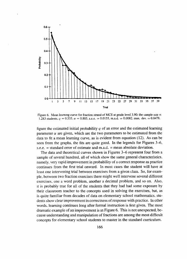
Figure 6. Mean learning curve for fraction strand of MCS at grade level 3.90; the sample size IS

1.283 students. y = 0.533. (Y = 0.885. s.e.e. = 0.0155. m.a.d. = 0.0082. max. dev. = 0.0478.

figure the estimated initial probability q of an error and the estimated learning parameter CY are given, which are the two parameters to be estimated from the data to fit a mean learning curve, as is evident from equation (12). As can be seen from the graphs, the fits are quite good. In the legends for Figures 3-6, s.e.e. = standard error of estimate and m a d . = mean absolute deviation.

The data and theoretical curves shown in Figures 3-6 represent four from a sample of several hundred, all of which show the same general characteristics. namely. very rapid improvement in probability of a correct response as practice continues from the first trial onward. In most cases the student will have at least one intervening trial between exercises from a given class. So, for exam- ple, between two fraction exercises there might well intervene several different exercises. one a word problem, another a decimal problem, and so on. Also. I t is probably true for all of the students that they had had some exposure by their classroom teacher to the concepts used in solving the exercises, but, as is quite familiar from decades of data on elementary school mathematics, stu- dents show clear improvement in correctness of response with practice. In other words, learning continues long after formal instruction is first given. The most dramatic example of an improvement is In Figure 6. This is not unexpected, be- cause understanding and manipulation of fractions are among the most difficult concepts for elementary school students to master in the standard curriculum.

166

In Figures 7-10 data from the same four classes of exercise are analyzed in terms of the more demanding requirement on the learning model to fit the sequential data. For learning theorists the stringency of the test to fit such sequential data with only three parameters is well known. The data in each of the figures have twelve degrees of fre;dom because of the three parameters estimated from the data. The largest x is for the multiplication exercises, byt even here the x is not significant at the O. 10 level, which is indicative of the good fits. Moreover, parameters of q and a were estimated only from the mean learning curve data. Only the parameter w was directly estimated from the sequential data. So the test of fit is a stringent one.

Modijication of Model III. In examining the fit of a number of mean learning curves, we found that by changing the time scale monotonically, the fit could sometimes be improved. In particular, we modified the mean learning curve given in (12) by replacing the exponent n of a, where, of course, n is the number of trials by n ß , so that we may write the equation for mean learning as:

(22) B 4n = a n 9 .

In Figures 1 1 and 12, we show comparative results for one class of exercise ' in division at the third grade level. In Figure l 1, the value of p is 1.0, and

in Figure 12, p is 1.258. The improvement in fit from using the second p is

1111 1110 1101 1 1 0 0 1011 IO10 1 0 0 1 l o00 o111 0110 0101 o100 O011 0010 o 0 0 1 OOOO

Figure 7. Joint probabllity of res onses on first four exercises. addition strand at gradeAlevel 3.10; o = O . 112, xP= 14.2. Observed data shown by black dots.

167

0.4 -

0.3 -

b

1 0.2

-

0.1 -

1111 1110 1101 1 1 0 0 lali IO10 l o o t lo00 o111 0110 0101 OIO0 O011 O010 ml oooo

Figure 8. Joint probability of responses on first four exercises, subtraction strand at grade level 4.10; W = 0.219, x 2 4.9.

1111 III0 1101 1 1 0 0 loll IO10 1001 l o 0 0 O l l 1 0110 0101 0100 O 0 1 1 0010 o 0 0 1 oooo

Figure 9. Joint probabdity of responses on first four exercises, multiplication strand at grade level 3.55; W = O.OO0, x 2 16.9.

168

0.2

b - 9 0.1 z P

l l

-_- I l l1 1110 1101 1 1 0 0 1011 1010 1 0 0 1 l o 0 0 O l l 1 0110 0101 o100 O011 0010 o 0 0 1 oooo

Figure 10. Joint probability of responses on first four exercises, fraction strand at grade level 3.90; W = 0.126, x 2 = 14.7

Tnal

Figure 1 1 . Mean learning curve for division strand of MCS at grade level 3.80; the sample size is 653 students. q = 0.516, a = 0.878. s.e.e. = 0.021, m.a.d. = 0.013, max. dev. = 0.074.

169

Trial

Figure 12. Same data for division as Figure 1 1 , but addmonal parameter B of equation (22): q = 0.480, (r = 0.935, = 1.258, s.e.e. = 0.0172. m.a.d. = 0.010, max. dev = 0.069.

visually apparent, also clearly in the comparative standard errors of estimates (s.e.e.) and mean absolute deviation (m.a.d.). But the improvement is, all the same, not large. So continued use of b = 1.0 is reasonable, for monotonic adjustments in the time scale are not easily dealt with at a fundamental level.

5. mAJECTORIES: THEORY

We now present an approach to evaluation of curriculum that we have been de- velopmg since the mid 1970s (the first article in the series is Suppes, Fletcher, and Zanotti, 1976). An extension of this work is to be found in Suppes, Macken, and Zanotti ( 1978), in Larsen, Markosian, and Suppes (1978), and in Malone, Suppes, Macken, Zanotti, and Kanerva (1979). The third of these articles (Larsen et af.) applied the theory of trajectories to a very different popula- tion, namely, undergraduates in a computer-based course in logic at Stanford. Extensive subsequent work has been done over the past twenty years at CCC originally under our joint direction and for the past five years under the guid- ance of the second author, Mario Zanotti. The empirical data we use here come from the extensive work at CCC. We turn now to a general introduction to this aspect of curriculum.

170

Many of US who 6ave engaged in currhdum reform efforts have been dissat- isfied with the wait-and-see approach required when classical evaluation of a new curriculum is used. We have in mind evaluation by comparing pretests and posttests, with an analysis of posttest grade placement distributions as a function of pretest distribution and exposure in s m e form to .the new curriculum.

In line with approaches used in other parts of science, it is natural to ask if a more predictive-control approach could be used and made an integral part of the curriculum to ensure greater benefits, especially for the students not close to the mean performance. The approach discussed in this chapter is aimed precisely at this question. The strategy is to develop a theory of prediction for individual student progress through the curriculum, to use this predictive mechanism as a means of control by regulating the amount of time spent on the curriculum by a given student, and thereby to achieve set objectives for the grade-placement gains of the student. Such an approach also calls for individualization in the objectives of a course, for it is unrealistic to expect all students to make the same gains in the same amount of time, or to expect that the slowest students can cover as much material as the best students simply by spending additional time. Consequently, even with a differential approach to the amount of time each student may spend in the curriculum, it is still not reasonable to impose a uniform concept of grade placement gain on all students.

Another important feature of our approach to the prediction of student pro- gress is to separate the global features of the curriculum from the global individ- ual parameters characterized for the individual student by a simple differential equation. In many respects, the estimation of the global individual parameters corresponds to the fixing of boundary conditions in the solution of differential equations in physics. In our case, the boundary conditions correspond to the characteristics of the individual student and the differential equation itself to the structure of the curriculum.

As we have already emphasized, our analysis is aimed at the global perfor- mance of the student. The fact that we are considering only global progress, and not performance on individual exercises, makes it possible for us to state gen- eral axioms about information processing from which we may derive the basic stochastic differential equation that we Selieve is characteristic of many different curriculums, especially curriculums that are tightly articulated and organized in their development. Certainly this is a characteristic of the computer-assisted instruction in elementary mathematics considered here.

Let us assume, as already indicated, that the student is progressing individ- ually through a course, and let I ( t ) be the total information presented to the student up to time t . We say here total information but we could also give a formulation in terms of concepts or skills and think of the development proce- durally rather than declaratively. Let y ( t ) be the student’s course position at

171

time t. Note that fa?. simplification of notation we have omitted a subscript for a particular student. It is understood that the notation used here applies only to an individual student not to averages of students. The stochastic averaging involved is averaging over the variety of skills or information presented to the student and refer to the student’s mean position and mean information. We shall not make these stochastic assumptions explicit any further, because only the mean theory for the individual student will be developed here.

The first assumption is that the process is additive using for simplicity of concept a discrete-time variable n. We may write the additivity assumption as follows:

(23) Additive: I (n ) - I (n - 1) = a,

which we can then express in terms of a derivative for continuous time as:

We then make the second strong assumption that the position in the course is proportional to the information introduced, that is,

Combining (24) and (25) we have:

which we then integrate to obtain:

(27) lny(t) = klnt + lnb,

(28) y(t) = btk.

which we may express so that y (t) is a power function of t:

We use parameters b and k to fit the shape of a student trajectory. We add another parameter a to use in estimating the student’s starting, grade placement position, so that our final equation is

(29) y(t) = btk +a.

6. TRAJECTORIES: DATA

We now turn to the analysis of a rather large number of student trajectories based on data collected in CCC’s courses in elementary mathematics and reading. We examine data on 1,485 students collected during the 1992-1993 school year from students in various parts of the United States.

172

d

Grade level gam

c 4 w

Tlmc Spent (mlnutes)

Figure 13. Example of three student trajectories.

400-

350 --

300 --

%=O

E 150 --

- -

am --

l o o --

so -- 53

O 1

I I

850 lo00 1150

368 -

262

1300 1450

109

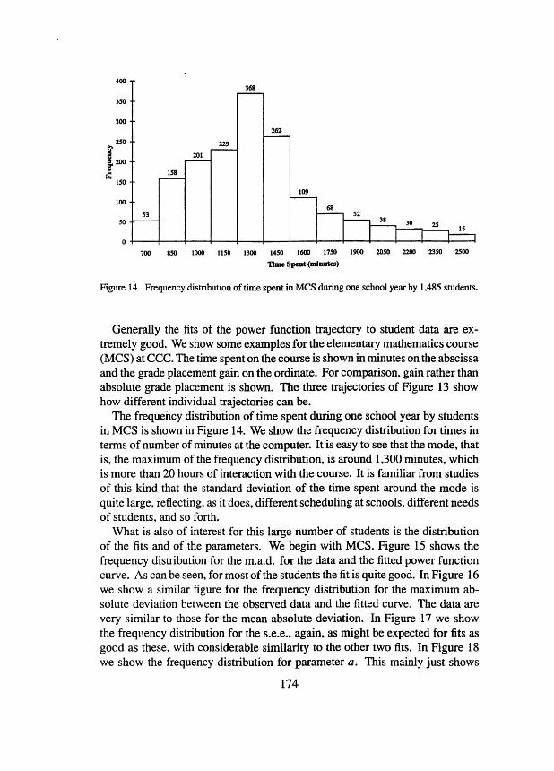
Figure 14. Frequency distnbutlon of time spent in MCS during one school year by 1,485 students.

Generally the fits of the power function trajectory to student data are ex- tremely good. We show some examples for the elementary mathematics course (MCS) at CCC. The time spent on the course is shown in minutes on the abscissa and the grade placement gain on the ordinate. For comparison, gain rather than absolute grade placement is shown. The three trajectories of Figure 13 show how different individual trajectories can be.

The frequency distribution of time spent during one school year by students in MCS is shown in Figure 14. We show the fiequency distribution for times in terms of number of minutes at the computer. It is easy to see that the mode, that is, the maximum of the frequency distribution, is around 1,300 minutes, which is more than 20 hours of interaction with the course. It is familiar from studies of this kind that the standard deviation of the time spent around the mode is quite large, reflecting, as it does, different scheduling at schools, different needs of students, and so forth.

What is also of interest for this large number of students is the distribution of the fits and of the parameters. We begin with MCS. Figure 15 shows the frequency distribution for the m.a.d. for the data and the fitted power function curve. As can be seen, for most of the students the fit is quite good. In Figure 16 we show a similar figure for the frequency distribution for the maximum ab- solute deviation between the observed data and the fitted curve. The data are very similar to those for the mean absolute deviation. In Figure 17 we show the frequency distribution for the s.e.e., again, as might be expected for fits as good as these, with considerable similarity to the other two fits. In Figure 18 we show the frequency distribution for parameter a. This mainly just shows

174

350 -

300 - -

250 - -

pz00 -- c E 150

- -

l o o --

so -- IO

O-

O 006

161

.L

298 307

0009 0012

241

0015 O018

ll.

o021 om 0.027 0.030 0.033 o m 6 o m 9 0.042 004s Absolute Mean Deviation

Figure 15. MCS frequency distribution of the m.a.d. for the fit of the 1,485 power function curves to the data.

o MO

143 -

184

+

212

7 170

197

h 82

18

1026 0032 0.038 0044 0030 0056 0062 0068 0074 0080 0086 0092 0098 0104 Oll0

Maaimum Deviation

Figure 16 MCS frequency distnbution of the m a d . for the fit of the 1,485 power function curves to the data.

at what grade level the students began. As can be seen, the students in the sample range from beginning first graders to seventh graders with the mode in the third grade. Figure 19 shows the frequency distribution for the parameter k , the exponent in the power function. For estimates based on a large number of data points and for any extended time, we would be surprised to have estimates for k > 1. As can be seen, there are more than three hundred in our sample,

175

332 315

-

221

O 0 2 4

~ 1 6

O 0 2 8 0032 0036 OMO O w 4 0048 0008 O012 0016 0020

Standard Error of Estimalion

Figure 17. MCS frequency distrlbutlon of the s.e.e. for the fit of the 1,485 power function curves to the data.

204 -

- 4.0

1%

1 l 5 2 0

L 5 0 5 5 6 0 6 5 7 0 7 5

104

53

3 5 4 5 2 5 3 0 5 0 5 5 6 0 6 5 7 0 7 5 O0 o 5 1 0

Inftlal Grade Level a

Figure I8 MCS frequency dlstrlbutlon of the estlrnated pararne for 1.485 students.

ter u In the power functlon curve

and these estimates arise when we are working from an initial segment when students often show an accelerated rate of learning and therefore have an esti- mate of k > l . We would not expect these large estimates of k to extend over a substantla1 part of the school year. What is important about the figure is to show how great the range of k is. If we exclude the two tails the range is from 0.4 to 1.4, a difference that leads to very considerable differences in rates of progress corresponding to rates of learning. We emphasize, on the other hand. that the

176

1 141

0 2 0.3 0 4 O 5

161

- 0 6

176 164 -

- 0 7

199

157 - 156 -

1 2 1 3 1.4 1 5 08 o 9 1 0 1 1

k

Figure 19. MCS frequency distribution of the estlmated parameter k in the power function for l .485 students.

loo0

900

- so0

-- --

700 - -

h 600 -- I; t 500 -- P w - -

300

m --

-- ~ 161

O 0.005 O 0 1 O015 O02 O025 O03 0035 O 0 4 0045 005 0055 006 0065 007 0075

b

Figure 20. MCS frequency dlstnbution of the parameter b in the power function for 1,485 students.

existence of such large individual differences in the student population is to be found in almost every other kind of estimation of achievement. But ordinarily these measures of achievement are for static cross-sectional tests, not for rates of progress during a period of at least several months.

In Figure 20 we show the distribution of the parameter b, which , unlike k , has a relatively small standard deviation around the mean value of approxi- mately 0.005. Again, it is the exponent k that reflects strongly the individual

263

386

700 850 loo0 1150

345

l I 157

1300 1450 1 6 0 0 1750 1900 2050 2200 2350 2500

n m e spent (*UW

700

600

500

300

!l 27

652

475 r 0.006 0.009 O012 O 015 0.018 0.021 0.024 0.027 O M O 0033 O 036

Absolute M m Deviation

Figure 22. RW frequency of m.a.d. of the fit of the 1,485 power functlon curves to the data.

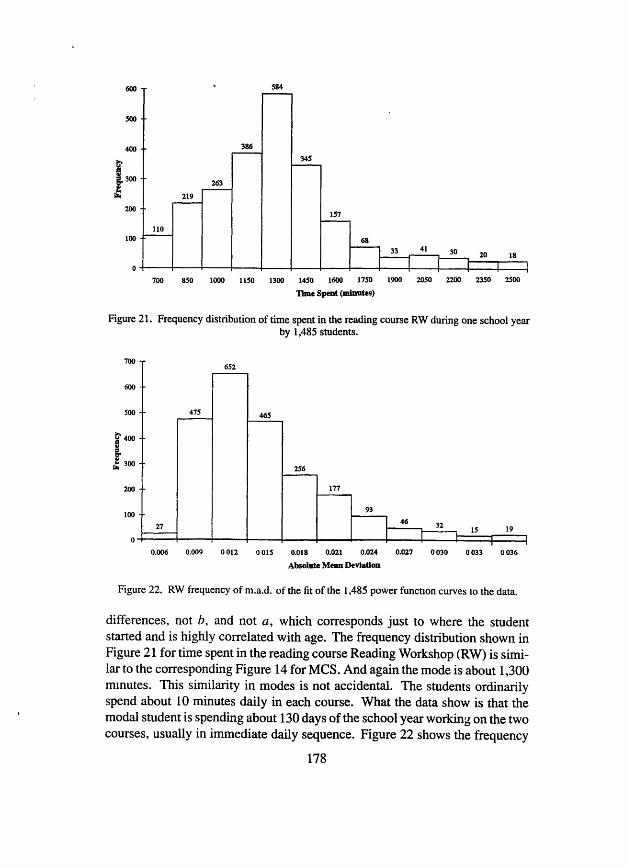
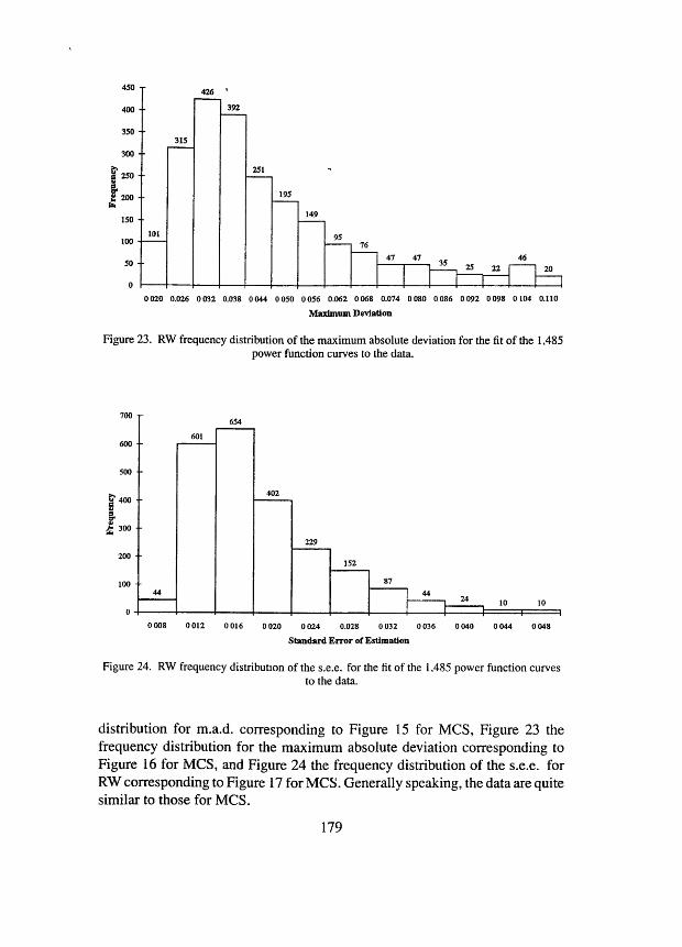
differences, not b, and not a, which corresponds just to where the student started and is highly correlated with age. The frequency distribution shown in Figure 21 for time spent in the reading course Reading Workshop (RW) îs simi- lar to the corresponding Figure 14 for MCS. And again the mode is about 1,300 mmutes. This similarity in modes is not accidental. The students ordinarily spend about 10 minutes daily in each course. What the data show is that the modal student is spending about 130 days of the school year working on the two courses, usually in immediate daily sequence. Figure 22 shows the frequency

178

315 350

426

392

7 95 , 76

46

O M O 0.026 O032 0.038 O 0 4 4 O 050 O056 0.062 O O68 0.074 O O80 O 086 O 092 O098 O 104 0.110

Maximum Deviation

Figure 23. RW frequency distribution of the maximum absolute deviation for the fit of the 1,485 power function curves to the data.

700 -

600 .-

500 .-

i 4 0 0

- - f 300

-- g

m - -

l o o - - 44

o ,

601

654

O008 0012 0016

402 1 229 , 152

87 44 t 24 10 10

1

OMO 0024 0.028 0032 OM6 0040 O 0 4 4 0048

Standard Error of Estimation

Figure 24. RW frequency distribution of the s.e.e. for the fit of the i ,485 power function curves to the data.

distribution for m.a.d. corresponding to Figure 15 for MCS, Figure 23 the frequency distribution for the maximum absolute deviation corresponding to Figure 16 for MCS, and Figure 24 the frequency distribution of the s.e.e. for RW corresponding to Figure 17 for MCS. Generally speaking, the data are quite similar to those for MCS.

179

450 - 400 -- 350 -- 300 --

$250 --

rb -- 150

- - so

-- 100

--

12 O

2 5

354 359

41 1

1

3 3 0 ~

3.0 3 5 4 O 4 5 5.0 5.5 6.0

Wal Grade Levd a

"t; 3

6.5 7.0 7.5

Figure 25. RW frequency distribution of the estimated parameter a in the power function curve for 1,485 students.

700

600

500

! 400

F 300

m

100

O

0.5 O6 0 7 08 O 9 1.0 1 1 1.2 13 1.4 1 5

k

Figure 26. RW frequency distnbution of the estimated parameter k m the power function curve for 1,485 students.

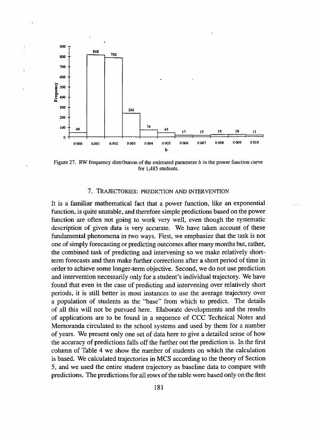
The similarity to MCS is also to be found in the distribution of the parameter a for RW, as shown in Figure 25. On the other hand, the distribution of the exponential parameter k is less spread out in the case of RW than in the case of MCS, as may be seen from Figure 26 in comparison with Figure 19. We have conjectures for this rather striking difference in the two courses, but we are not certain of their correctness. Finally, in Figure 27 we show the distribution for RW of the parameter b, which again is similar to that for MCS (Figure 20) but has a smaller value for the mode and a slightly larger standard deviation.

180

700

300

m

100

o , I

0000 0.001 0.002 O003 0004 0005 0006 0007 0008 O009 0010

b

Figure 27. RW frequency distribution of the estimated parameter b in the power function curve for 1,485 students.

7. TRAJECTORIES: PREDICTION AND INTERVENTION

It is a familiar mathematical fact that a power function, like an exponential function, is quite unstable, and therefore simple predictions based on the power function are often not going to work very well, even though the systematic description of given data is very accurate. We have taken account of these fundamental phenomena in two ways. First, we emphasize that the task is not one of simply forecasting or predicting outcomes after many months but, rather, the combined task of predicting and intervening so we make relatively short- term forecasts and then make further corrections after a short period of time in order to achieve some longer-term objective. Second, we do not use prediction and intervention necessarily only for a student’s individual trajectory. We have found that even in the case of predicting and intervening over relatively short periods, it is still better in most instances to use the average trajectory over a population of students as the “base” from which to predict. The details of all this will not be pursued here. Elaborate developments and the results of applications are to be found in a sequence of CCC Technical Notes and Memoranda circulated to the school systems and used by them for a number of years. We present only one set of data here to give a detailed sense of how the accuracy of predictions falls off the further out the prediction is. In the first CS~UIIUI of Table 4 we show the number of students on which the calculation is based. We calculated trajectories in MCS according to the theory of Section 5, and we used the entire student trajectory as baseline data to compare with predictions. The predictions for all rows of the table were based only on the first

181

8 Table 4. Data analysis on predicted trajectories of individual students, based on

theirjrst 600 minutes of computer-based instruction.

N Time Diff. S .D.

705 600 0.026 0.027 659 700 0.040 0.040 595 800 0.058 0.055 515 900 0.078 0.072 436 1,000 o. 100 0.092 3 84 1,100 0.121 0.1 11 33 1 1,200 0.145 0.132 278- 1,300 0.171 0.152 233 1,400 0.20 1 O. 177 196 1,500 0.237 0.209 170 1,600 0.27 1 0.237 137 1,700 0.297 0.270 104 1,800 0.325 0.295 88 1,900 0.344 0.33 1 72 2,000 0.377 0.345

~~ _ _ _ _ ~ ~~

600 minutes. In each row we are comparing the predicted grade placement after x minutes for the students who had during the school year at least that many minutes of computer time, with the grade placement inferred from the trajectory fitted to all the data. We used the trajectory fitted to all the data to provide the data point to compare with prediction, because we did not have direct observations of grade placement every 100 minutes. As is evident, we show cumulative time in column 2 of Table 4, and the mean absolute difference between the predicted and data-fitted grade placements in column 3. In column 4 we show the corresponding standard deviation for the predicted and data-fitted grade placements. We emphasize again that the predictions for all rows were based on the data-fitted trajectory for the first 600 minutes, so both columns 2 and 3 show, as expected, monotonically increasing deviations between prediction and data fit as the point of prediction of grade placement is further away from the initial 600 minutes.

8. MOVEMENT AND MASTERY: NEW VERSION

In this section we turn to our conceptualization of student movement and mas- tery criteria for a new course at Stanford tRat includes not only review and practice, but also short “audiovisual lectures” on each major concept as it is in- troduced. In other words, we now turn to the problem of movement and mastery

182

in what is meant to be a self-contained course in elementary mathematics for grades K-8. In the context of the present analysis we shall not really discuss the content of the course, which is based on an extensive revision of the first au- thor’s elementary mathematics textbock series Set$ and Numbers (1963). Here we only want to concentrate on drawing lessons from our experience with the mathematics concepts and skills course at CCC and related courses, as well as our work in other areas on learning, to design a new and, we believe, still more dynamic approach to problems of movement and mastery.

We begin with the classification of each trial, or, if you will, each exercise, into one of eight types. This partition of exercises is, of course, not the most refined one, but we believe it constitutes a sufficiently fine partition for purposes of making conceptual distinctions about learning and forgetting, and at the same time is not so fine but that we can seriously track individual students at each stage in terms of a parameterized version of these eight kinds of learning and forgetting. Notice that Learning Model III is incorporated quite directly into this classification. The model of forgetting goes back to earlier work (Suppes, 1964). As far as we know, the explicit introduction of models of forgetting in the analysis and management of computer-based curriculum has not previously taken place, even though in many kinds of instruction intuitive and implicit assumptions about forgetting are made, as for example in the various regimes of review and practice that are set up.

I . Movement and computation of q n

Beginning with the first learning trial on a given concept C I , any later trial on any task or concept has one of the following classifications with respect to concept C,, as long as C, is in the active set A (see III. 5 and V. 1). The model and parameters of change of q,, for each of the eight types are shown after the description. Remember, qn is the probability of an error on concept C, on trial n -we omit for simplicity the subscript i on q, which is understood.

1. A learning trial on C, with a correct response

q n f l = (1 - d a q n .

2. A learning trial on C, with a wrong response

q n + l = ( 1 - m)Crqn + a m .

3. A review trial on C, with a correct response

qn+ l (1 - @>&n.

4. A review trial on C, with a wrong response

qn+ l = (1 - m)Bqn + P m -

183

5.

6.

7.

8.

1.

2.

3.

4.

5 .

A “same strand” trial on a concept that has Ci as a prerequisite and a correct response

qn+1 = a4n.

A “same strand” trial on a concept that does not have Ci as a prerequisite, but a correct response.

qn+l = S q n .

For a “same strand” trial, if the response is incorrect,

qn+1 = q n -

An “other” trial on a strand to which Ci does not belong

qn+1 = (1 - +?n + 6-

II. Criterion of movement

Grade placement of concepts. Each concept C, of each strand i has a grade placement GP(Ci). Example, GP(C,) = 4.50. The integer 4 is the grade and S O is the position of this concept in the fourth grade. At any time, a student has a current grade placement in each strand, which we express as GP(i, s). This current GP(i, s) shows what concept the student is working on in strand i . Let

GP(i*, s) = myc GP(i, s),

that is, i* is the strand in which student s currently has the highest grade placement. There can be several strands at the same position, so the max does not have to be unique. For each strand i, let N ( i , s) be the number of concepts between GP(i, s) and GP(i*, s). (a) If GP(i*, s) - GP(i, s) =- O, take the number to be at least 1. (b) Because the number of concepts varies in different strands, the count of

number of concepts between the two grade placements GP(i*, s) and GP(i, s) is a better measure of curriculum to be covered in strand i than is the numerical difference GP(i*. s) - GP(i, s).

We use N ( i , s) to compute a current probability distribution of curriculum emphasis for student s - as can be seen, this probability distribution varies from one student to another, and from one time to another for the same student. (a) ~ ( s ) = C N ( ~ , s).

l

1

184

(b) P ( ì , s> = N ( ì , s ) / N (s) if N ( s ) > O. Use the rational fractions p ( i , s) to choose probabilistically the next strand i, sampling with replacement.

(c) If N (s) = O, that is, all strands have the same GP(i, s), use the uniform distribution, that is, weight all strands equally, in choosing the next ~

strand.

grade placement.

P

(d) Use the uniform distribution initially when all strands have the same

6. Choice of learning L or review R after choice of strand i. (a) If no concepts of strand i are in active set A such that qr,n q*, go to

(b) Let j =I Ai I be cardinality of concepts in A from strand i such that next new concept C,.

where q* is parameter for review. By assumption j > O. (c) Choose R with probability j / ( j + 1). (d) Choose L then with probability 1 - [ j / ( j + l)]. (e) Having chosen R, review concept C, in A that has maximum qi,n- if a

(f) If L is chosen, then, as already stated, go to next concept C, in strand i tie, choose randomly among the maximum set.

for student s.

III. Criterion of learning

1. On initial presentation of a concept, choose exercises by a slightly modified Fibonacci sequence, for example, Differences: 1,2,3,5,8,13 Exercise no.: 1,3,6,11,19,32.

2. If mastery does not result from a Fibonacci sequence on first block, then -7

run a Fibonacci sequence again on the remaining sequence of exercises not used the first time.

3. On any learning trial, if

then the mastery criterion, as determined by the parameter m, is satisfied. 4. If the mastery criterion is not met, continue learning trials until no trials are

left. 5. Whether either 3 or 4 obtains, after learning trials end, put C, in active set

A.

185

IV. Choice of review exercises

1. When a concept Ci is selected for review from active set A , randomly choose two exercises from the learning exerdses following this concept.

2. If both exercises have wrong response, go to lecture on Ci and then ran- domly choose two other exercises from the learning exercises following this -

concept. But go as part of review of lecture L on C, a maximum of A times. 3. Otherwise go back to Section II and choose a strand i , then L or R as before.

K Removal of concept from active list A

1. If C, from strand i is in A , remove from A if and only if

GP(i, S) - GP(C,) > y ,

where

GP(i, s) = grade placement of student s on strand i GP(C, ) = grade placement of concept C, in the curriculum.

We ordinarily take y = 0.5, a half-year in grade placement.

VI. Updated GP(i, s)

Every time a new concept C, is introduced to a student, GP(i, s) is then updated to the position of C,, that is,

GP(i, s ) = GP(C,).

(This remains true even when a concept C, is failed in the present version.)

VII. Initial rTalues of parameters for first experiment

q = S , CY = .9, W = . l , m = .23,ß = .8 6 = .001,6* = 82 = .99, q* = .3, y = s , h = 2.

9. CONCLUDING REMARKS

A quick inspection shows that this new version of mastery learning differs in significant ways from what is described in earlier sections and has been used extensively in CCC courses. Obviously some ingredients of the new system are based on more recent scientific results than others. Perhaps the most important feature of which this is true is the forgetting model embodied in the eighth type

186

Of movement undei1 at the beginning of Section 8, that is, the equation

q,+1 = (1 - d q n + € 9

which applies to a trial presenting an exercise not belonging to the strand to which Ci belongs. This equation prmides a ve@ simple model of forgetting- the probability of error increases slightly when other exercises from another strand are given. The model is, of course, much too simple. We woÚld naturally expect forgetting to vary significantly as a function of both student and concept. As new data accumulate, we hope to at least introduce a parameter for each student and each strand.

A critical dynamic feature of the new version is the active set A of concepts to be reviewed, especially the subset A* of A whose error rates are above the criterion q* according to the model computations used. Computing the expected size of A or A* as a function of the model parameters is too complex to be feasible, but we have simulated the system with the parameters shown in VIL

We believe that the dynamic features we have built into the review process should accommodate a broad range of data and models concerned with forget- ting. We also emphasize that it is most desirable that the models used go beyond the phenomenological data of forgetting to the causes of the phenomena, causes that have been much studied in the experimental literatures of psychology over many years, but hardly used at all in quantitative approaches to curriculum organization.

The third, and final, critical aspect of the new version we consider is the method of tutorial intervention. In the version being implemented and tested at Stanford in the spring of 1995, we have restricted tutorial intervention to that given in IV. 2, which is to return the student to the instructional lecture on a concept when difficulties arise in doing the relevant review exercises. In the future, we plan to add new, brief tutorial lectures on concepts that seem to require it, as judged by the performance of the students. Second, we plan to add brief tutorial interventions for particular exercises that students get wrong with high probability and for reasons we can diagnose.

These remarks touch on only a few of the many ideas we have for improve- ment. Students and their parents are already suggesting many other features they would find attractive. It is part of our Bayesian viewpoint outlined at the beginning of this article that there is no end to such improvements. It is particu- larly important for us to stress the importance of revisions based on systematic theory and data, even though we do not expect the results in any sense to be able fully to dictate the changes. A Bayesian place for intuitive judgment must remain, even as we struggle to develop our theoretical ideas ever more thor- oughly and in close conjunction with an explicit articulation of learning goals for individual students.

187

REFERENCES

Karlin, S.: 1953. Some random walks arising in learning models, Part I. Pacific Journal of Mathe- matics, 3,725-756.

Larsen, I., Markosian, L. Z., and Suppes, P.: 1978. Performance models of undergraduate students on computer-assisted instruction in elementary logic. Instructional Science, 7, 15-35.

Malone, T. W., Suppes, P., Macken, E., Zanotti, M., and Kanerva, L.: 1979. Projecting student tra- jectories m a computer-assisted instruction curriculum. Journal of Educational Psychology, 71,74-84.

Suppes, P.: 1964. Problems of optimization in leaming a list of simple items. In M. W. Shelly II and G. L. Bryan (Eds.), Human Judgments and Optimaliry, New York: Wiley, 1 16-126.

Suppes, P.: 1967. Some theoretical models for mathematics learning. Journal of Research and Development in Education, 1,5-22.

Suppes, P.: 1972. Computer-assuted instruction. In W. Handler and J. Weizenbaum (ms.), Display Use for Man-Machine Dialog. Munich: Hanser, 155-185.

Suppes, P., Fletcher, J. D., and Zanotti, M.: 1976. Models of individual trajectories in computer- assisted instruction for deaf students. Journal of Educational Psychology, 68, 1 17-127.

Suppes, P., Groen, G., and Schlag-Rey, M.: 1966; A model for response latency in paired-associate learning. Journal of Mathematical Psychology, 3: 1.99-128.

Suppes, P., Macken, E., and Zanotti, M.: 1978. The role of global psychological models in in- structional technology. In R. Glaser (Ed.), Advances m Instructlonu1 Psychology, Vol. l . Hillsdale, NJ: Erlbaum, 229-259.

Suppes, P., and Momingstar, M.: 1972. Computer-Assisted Instruction at Stanford, 1966-68. Data, Models. und Evaluation of the Arithmetic Programs. New York: Academlc Press.

Teachers Handbook for Math Concepts and Skills. Computer Curriculum Corporatlon, 1993.

188