Embed Size (px)
Citation preview
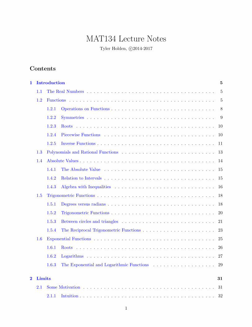
MAT134 Lecture NotesTyler Holden, c©2014-2017
Contents
1 Introduction 5
1.1 The Real Numbers . . . . . . . . . . . . . . . . . . . . . . . . . . . . . . . . . . . . . 5
1.2 Functions . . . . . . . . . . . . . . . . . . . . . . . . . . . . . . . . . . . . . . . . . . 5
1.2.1 Operations on Functions . . . . . . . . . . . . . . . . . . . . . . . . . . . . . . 8
1.2.2 Symmetries . . . . . . . . . . . . . . . . . . . . . . . . . . . . . . . . . . . . . 9
1.2.3 Roots . . . . . . . . . . . . . . . . . . . . . . . . . . . . . . . . . . . . . . . . 10
1.2.4 Piecewise Functions . . . . . . . . . . . . . . . . . . . . . . . . . . . . . . . . 10
1.2.5 Inverse Functions . . . . . . . . . . . . . . . . . . . . . . . . . . . . . . . . . . 11
1.3 Polynomials and Rational Functions . . . . . . . . . . . . . . . . . . . . . . . . . . . 13
1.4 Absolute Values . . . . . . . . . . . . . . . . . . . . . . . . . . . . . . . . . . . . . . . 14
1.4.1 The Absolute Value . . . . . . . . . . . . . . . . . . . . . . . . . . . . . . . . 15
1.4.2 Relation to Intervals . . . . . . . . . . . . . . . . . . . . . . . . . . . . . . . . 15
1.4.3 Algebra with Inequalities . . . . . . . . . . . . . . . . . . . . . . . . . . . . . 16
1.5 Trigonometric Functions . . . . . . . . . . . . . . . . . . . . . . . . . . . . . . . . . . 18
1.5.1 Degrees versus radians . . . . . . . . . . . . . . . . . . . . . . . . . . . . . . . 18
1.5.2 Trigonometric Functions . . . . . . . . . . . . . . . . . . . . . . . . . . . . . . 20
1.5.3 Between circles and triangles . . . . . . . . . . . . . . . . . . . . . . . . . . . 21
1.5.4 The Reciprocal Trigonometric Functions . . . . . . . . . . . . . . . . . . . . . 23
1.6 Exponential Functions . . . . . . . . . . . . . . . . . . . . . . . . . . . . . . . . . . . 25
1.6.1 Roots . . . . . . . . . . . . . . . . . . . . . . . . . . . . . . . . . . . . . . . . 26
1.6.2 Logarithms . . . . . . . . . . . . . . . . . . . . . . . . . . . . . . . . . . . . . 27
1.6.3 The Exponential and Logarithmic Functions . . . . . . . . . . . . . . . . . . 29
2 Limits 31
2.1 Some Motivation . . . . . . . . . . . . . . . . . . . . . . . . . . . . . . . . . . . . . . 31
2.1.1 Intuition . . . . . . . . . . . . . . . . . . . . . . . . . . . . . . . . . . . . . . . 32
1
2.2 One Sided Limits . . . . . . . . . . . . . . . . . . . . . . . . . . . . . . . . . . . . . . 35
2.3 Limit Laws . . . . . . . . . . . . . . . . . . . . . . . . . . . . . . . . . . . . . . . . . 37
2.4 The Squeeze Theorem . . . . . . . . . . . . . . . . . . . . . . . . . . . . . . . . . . . 40
2.5 Infinite Limits . . . . . . . . . . . . . . . . . . . . . . . . . . . . . . . . . . . . . . . . 42
2.5.1 Vertical Asymptotes . . . . . . . . . . . . . . . . . . . . . . . . . . . . . . . . 42
2.5.2 Horizontal Asymptotes . . . . . . . . . . . . . . . . . . . . . . . . . . . . . . . 44
2.6 Continuity . . . . . . . . . . . . . . . . . . . . . . . . . . . . . . . . . . . . . . . . . . 48
2.6.1 One-Sided Continuity and Failures of Continuity . . . . . . . . . . . . . . . . 52
3 Derivatives 53
3.1 First Principles . . . . . . . . . . . . . . . . . . . . . . . . . . . . . . . . . . . . . . . 53
3.1.1 The Geometry of the Derivative . . . . . . . . . . . . . . . . . . . . . . . . . 56
3.1.2 A Different Parameterization . . . . . . . . . . . . . . . . . . . . . . . . . . . 58
3.1.3 Relating Variables and Leibniz Notation . . . . . . . . . . . . . . . . . . . . . 59
3.2 Some Derivative Results . . . . . . . . . . . . . . . . . . . . . . . . . . . . . . . . . . 60
3.2.1 Linearity and the Power Rule . . . . . . . . . . . . . . . . . . . . . . . . . . . 60
3.2.2 The Natural Exponent . . . . . . . . . . . . . . . . . . . . . . . . . . . . . . . 62
3.2.3 The Product and Quotient Rule . . . . . . . . . . . . . . . . . . . . . . . . . 63
3.2.4 Higher Order Derivatives . . . . . . . . . . . . . . . . . . . . . . . . . . . . . 66
3.3 Trigonometric Derivatives . . . . . . . . . . . . . . . . . . . . . . . . . . . . . . . . . 66
3.3.1 Two Important Limits . . . . . . . . . . . . . . . . . . . . . . . . . . . . . . . 66
3.3.2 Differentiating Sine and Cosine . . . . . . . . . . . . . . . . . . . . . . . . . . 68
3.3.3 Degrees versus Radians . . . . . . . . . . . . . . . . . . . . . . . . . . . . . . 69
3.4 Smoothness of Differentiable Functions . . . . . . . . . . . . . . . . . . . . . . . . . . 69
3.4.1 Differentiable implies Continuous . . . . . . . . . . . . . . . . . . . . . . . . . 70
3.4.2 Failures of Differentiability . . . . . . . . . . . . . . . . . . . . . . . . . . . . 70
3.5 Chains and Inverses . . . . . . . . . . . . . . . . . . . . . . . . . . . . . . . . . . . . 73
3.5.1 The Chain Rule . . . . . . . . . . . . . . . . . . . . . . . . . . . . . . . . . . 73
3.5.2 Derivatives of Inverse Functions . . . . . . . . . . . . . . . . . . . . . . . . . . 77
3.5.3 The Inverse Trigonometric Functions . . . . . . . . . . . . . . . . . . . . . . . 79
3.5.4 Logarithmic Differentiation . . . . . . . . . . . . . . . . . . . . . . . . . . . . 81
2
4 Applications of Derivatives 82
4.1 Rates of Change . . . . . . . . . . . . . . . . . . . . . . . . . . . . . . . . . . . . . . 83
4.1.1 Gravity . . . . . . . . . . . . . . . . . . . . . . . . . . . . . . . . . . . . . . . 83
4.1.2 The Simple Harmonic Oscillator . . . . . . . . . . . . . . . . . . . . . . . . . 85
4.1.3 The Pendulum . . . . . . . . . . . . . . . . . . . . . . . . . . . . . . . . . . . 86
4.1.4 Exponential Growth . . . . . . . . . . . . . . . . . . . . . . . . . . . . . . . . 87
4.2 Implicit Differentiation . . . . . . . . . . . . . . . . . . . . . . . . . . . . . . . . . . . 91
4.2.1 The Idea of Implicit Functions . . . . . . . . . . . . . . . . . . . . . . . . . . 91
4.2.2 How Implicit Differentiation Works . . . . . . . . . . . . . . . . . . . . . . . . 92
4.3 Related Rates . . . . . . . . . . . . . . . . . . . . . . . . . . . . . . . . . . . . . . . . 94
4.4 L’Hopital’s Rule . . . . . . . . . . . . . . . . . . . . . . . . . . . . . . . . . . . . . . 97
4.4.1 Standard Indeterminate Type . . . . . . . . . . . . . . . . . . . . . . . . . . . 98
4.4.2 Other Indeterminate Types . . . . . . . . . . . . . . . . . . . . . . . . . . . . 101
4.5 Derivatives and the Shape of a Graph . . . . . . . . . . . . . . . . . . . . . . . . . . 103
4.6 First Derivative Information . . . . . . . . . . . . . . . . . . . . . . . . . . . . . . . . 103
4.6.1 Second Derivative Information . . . . . . . . . . . . . . . . . . . . . . . . . . 105
4.7 Maxima and Minima . . . . . . . . . . . . . . . . . . . . . . . . . . . . . . . . . . . . 108
4.7.1 Optimization . . . . . . . . . . . . . . . . . . . . . . . . . . . . . . . . . . . . 114
4.7.2 Curve Sketching . . . . . . . . . . . . . . . . . . . . . . . . . . . . . . . . . . 117
5 Integration 124
5.1 Sigma Notation . . . . . . . . . . . . . . . . . . . . . . . . . . . . . . . . . . . . . . . 124
5.2 The Definite Integral . . . . . . . . . . . . . . . . . . . . . . . . . . . . . . . . . . . . 127
5.2.1 The Intuition . . . . . . . . . . . . . . . . . . . . . . . . . . . . . . . . . . . . 127
5.2.2 Estimating Areas . . . . . . . . . . . . . . . . . . . . . . . . . . . . . . . . . . 128
5.2.3 Defining the Definite Integral . . . . . . . . . . . . . . . . . . . . . . . . . . . 131
5.3 Anti-Derivatives . . . . . . . . . . . . . . . . . . . . . . . . . . . . . . . . . . . . . . 134
5.4 The Fundamental Theorem of Calculus . . . . . . . . . . . . . . . . . . . . . . . . . . 137
5.4.1 Indefinite Integrals . . . . . . . . . . . . . . . . . . . . . . . . . . . . . . . . . 140
5.4.2 Integral Notation . . . . . . . . . . . . . . . . . . . . . . . . . . . . . . . . . . 141
6 Integration Techniques 142
3
6.1 Integration by Substitution . . . . . . . . . . . . . . . . . . . . . . . . . . . . . . . . 142
6.1.1 Definite Integrals . . . . . . . . . . . . . . . . . . . . . . . . . . . . . . . . . . 144
6.2 Integration by Parts . . . . . . . . . . . . . . . . . . . . . . . . . . . . . . . . . . . . 146
6.3 Integrating Trigonometric Functions . . . . . . . . . . . . . . . . . . . . . . . . . . . 150
6.4 Trigonometric Substitution . . . . . . . . . . . . . . . . . . . . . . . . . . . . . . . . 153
6.5 Partial Fractions . . . . . . . . . . . . . . . . . . . . . . . . . . . . . . . . . . . . . . 156
7 Applications of Integration 159
7.1 Area Computations . . . . . . . . . . . . . . . . . . . . . . . . . . . . . . . . . . . . . 159
7.1.1 What We Already Know . . . . . . . . . . . . . . . . . . . . . . . . . . . . . . 159
7.1.2 More Complicated Shapes . . . . . . . . . . . . . . . . . . . . . . . . . . . . . 160
7.1.3 Unsigned (Absolute) Area . . . . . . . . . . . . . . . . . . . . . . . . . . . . . 161
7.1.4 Integrating along the y-axis . . . . . . . . . . . . . . . . . . . . . . . . . . . . 163
7.1.5 The Area Between Curves . . . . . . . . . . . . . . . . . . . . . . . . . . . . . 165
7.2 Work and Mass . . . . . . . . . . . . . . . . . . . . . . . . . . . . . . . . . . . . . . . 167
7.2.1 Work . . . . . . . . . . . . . . . . . . . . . . . . . . . . . . . . . . . . . . . . 168
7.2.2 Mass . . . . . . . . . . . . . . . . . . . . . . . . . . . . . . . . . . . . . . . . . 170
7.3 Cross Sections . . . . . . . . . . . . . . . . . . . . . . . . . . . . . . . . . . . . . . . . 171
7.3.1 The Cross-Section Formula . . . . . . . . . . . . . . . . . . . . . . . . . . . . 172
7.3.2 Simple Cross-Sections . . . . . . . . . . . . . . . . . . . . . . . . . . . . . . . 173
7.3.3 Cross-Sections for Solids of Revolution . . . . . . . . . . . . . . . . . . . . . . 176
7.3.4 Area bounded by two curves . . . . . . . . . . . . . . . . . . . . . . . . . . . 177
7.3.5 Rotating about different axes . . . . . . . . . . . . . . . . . . . . . . . . . . . 179
7.4 Other Volumes . . . . . . . . . . . . . . . . . . . . . . . . . . . . . . . . . . . . . . . 181
7.4.1 Sweeping by Shells . . . . . . . . . . . . . . . . . . . . . . . . . . . . . . . . . 181
7.4.2 Shells with Other Bases . . . . . . . . . . . . . . . . . . . . . . . . . . . . . . 185
7.5 Improper Integrals . . . . . . . . . . . . . . . . . . . . . . . . . . . . . . . . . . . . . 186
7.5.1 Infinite Intervals . . . . . . . . . . . . . . . . . . . . . . . . . . . . . . . . . . 186
7.5.2 Unbounded Functions . . . . . . . . . . . . . . . . . . . . . . . . . . . . . . . 189
7.5.3 The Basic Comparison Test . . . . . . . . . . . . . . . . . . . . . . . . . . . . 191
7.5.4 The Limit Comparison Test . . . . . . . . . . . . . . . . . . . . . . . . . . . . 193
4
8 Sequences and Series 194
8.1 Sequences . . . . . . . . . . . . . . . . . . . . . . . . . . . . . . . . . . . . . . . . . . 194
8.1.1 Definition . . . . . . . . . . . . . . . . . . . . . . . . . . . . . . . . . . . . . . 194
8.1.2 Limits of Sequences . . . . . . . . . . . . . . . . . . . . . . . . . . . . . . . . 197
8.1.3 Theorems on Convergent Sequences . . . . . . . . . . . . . . . . . . . . . . . 200
8.2 Infinite Series . . . . . . . . . . . . . . . . . . . . . . . . . . . . . . . . . . . . . . . . 203
8.2.1 Definition . . . . . . . . . . . . . . . . . . . . . . . . . . . . . . . . . . . . . . 203
8.2.2 Some Special Series . . . . . . . . . . . . . . . . . . . . . . . . . . . . . . . . 204
8.3 Convergence Tests . . . . . . . . . . . . . . . . . . . . . . . . . . . . . . . . . . . . . 207
8.3.1 The Integral Test . . . . . . . . . . . . . . . . . . . . . . . . . . . . . . . . . . 208
8.3.2 Comparison Tests . . . . . . . . . . . . . . . . . . . . . . . . . . . . . . . . . 210
8.3.3 Alternating Series and Absolute Convergence . . . . . . . . . . . . . . . . . . 213
8.3.4 Non-Comparison Tests . . . . . . . . . . . . . . . . . . . . . . . . . . . . . . . 216
9 Power Series 218
9.1 Radius of Convergence . . . . . . . . . . . . . . . . . . . . . . . . . . . . . . . . . . . 219
9.2 Differentiation and Integration of Power Series . . . . . . . . . . . . . . . . . . . . . 222
9.3 Taylor Series . . . . . . . . . . . . . . . . . . . . . . . . . . . . . . . . . . . . . . . . 223
9.3.1 Taylor Polynomials . . . . . . . . . . . . . . . . . . . . . . . . . . . . . . . . . 223
9.3.2 Taylor Series . . . . . . . . . . . . . . . . . . . . . . . . . . . . . . . . . . . . 225
9.4 Differentiation and Integration of Taylor Series . . . . . . . . . . . . . . . . . . . . . 227
9.5 Applications of Taylor Series . . . . . . . . . . . . . . . . . . . . . . . . . . . . . . . 228
5
1 Introduction
1 Introduction
We begin with a very rapid review of some pre-calculus concepts. It is essential that the studentmaster these ideas before we begin studying calculus proper.
1.1 The Real Numbers
The real numbers are our focus in this course, or rather functions which eat real numbers. Roughlyspeaking, the real numbers consist of all possible decimal expansions of numbers, and are denotedR. For example,
π,√
2, −17.37125
are real numbers.
As functions often act on large collections of numbers, we need a system for concisely describingintervals of such numbers. If a, b are real numbers with a < b, we use the following notation:
All x satisfying a < x < b by (a, b),
All x satisfying a ≤ x < b by [a, b),
All x satisfying a < x ≤ b by (a, b],
All x satisfying a ≤ x ≤ b by [a, b].
In particular, a parenthesis means that the endpoint is not included in the interval, while a squarebracket indicates that the endpoint is contained in the interval. We say that the interval (a, b) isan open interval and [a, b] is a closed interval. The intervals (a, b] and [a, b) may be referred to aseither half open or half closed. When we wish to indicate that x is simply less than or larger thana number, we include a ±∞ sign in the appropriate spot. For example,
All x satisfying x < a by (−∞, a),
All x satisfying x ≤ a by (−∞, a],
All x satisfying x > b by (b,∞),
All x satisfying x ≥ g by [b,∞).
Note that the infinity sign is always used in conjunction with an open bracket. If you are familiarwith the notion of unions and intersections, you can use these to combine intervals in a convenientway.
1.2 Functions
We think of a function as a machine which eats a number and produces another number. It isimportant that a function only produce a single output for each input. For example, the functionf(x) = x2 takes in an input x and produces the output x2.
6c©2013-2017 Tyler Holden
1.2 Functions 1 Introduction
Input Output
−2 40 0√2 2π π2
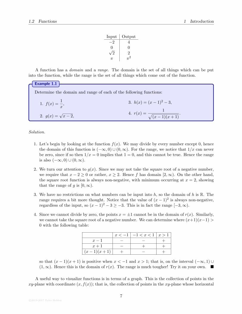
A function has a domain and a range. The domain is the set of all things which can be putinto the function, while the range is the set of all things which come out of the function.
Example 1.1
Determine the domain and range of each of the following functions:
1. f(x) =1
x,
2. g(x) =√x− 2,
3. h(x) = (x− 1)2 − 3,
4. r(x) =1√
(x− 1)(x+ 1).
Solution.
1. Let’s begin by looking at the function f(x). We may divide by every number except 0, hencethe domain of this function is (−∞, 0) ∪ (0,∞). For the range, we notice that 1/x can neverbe zero, since if so then 1/x = 0 implies that 1 = 0, and this cannot be true. Hence the rangeis also (−∞, 0) ∪ (0,∞).
2. We turn our attention to g(x). Since we may not take the square root of a negative number,we require that x− 2 ≥ 0 or rather, x ≥ 2. Hence f has domain [2,∞). On the other hand,the square root function is always non-negative, with minimum occurring at x = 2, showingthat the range of g is [0,∞).
3. We have no restrictions on what numbers can be input into h, so the domain of h is R. Therange requires a bit more thought. Notice that the value of (x− 1)2 is always non-negative,regardless of the input, so (x− 1)2 − 3 ≥ −3. This is in fact the range [−3,∞).
4. Since we cannot divide by zero, the points x = ±1 cannot be in the domain of r(x). Similarly,we cannot take the square root of a negative number. We can determine where (x+1)(x−1) >0 with the following table:
x < −1 −1 < x < 1 x > 1
x− 1 − − +
x+ 1 − + +
(x− 1)(x+ 1) + − +
so that (x− 1)(x+ 1) is positive when x < −1 and x > 1; that is, on the interval (−∞, 1) ∪(1,∞). Hence this is the domain of r(x). The range is much tougher! Try it on your own. �
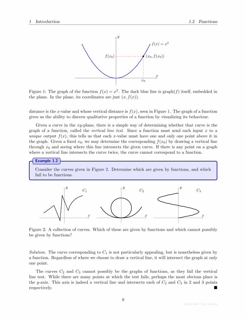
A useful way to visualize functions is in terms of a graph. This is the collection of points in thexy-plane with coordinate (x, f(x)); that is, the collection of points in the xy-plane whose horizontal
c©2013-2017 Tyler Holden
7
1 Introduction 1.2 Functions
x
y
f(x) = x2
x0
f(x0) (x0, f(x0))
Figure 1: The graph of the function f(x) = x2. The dark blue line is graph(f) itself, embedded inthe plane. In the plane, its coordinates are just (x, f(x)).
distance is the x-value and whose vertical distance is f(x), seen in Figure 1. The graph of a functiongives us the ability to discern qualitative properties of a function by visualizing its behaviour.
Given a curve in the xy-plane, there is a simple way of determining whether that curve is thegraph of a function, called the vertical line test. Since a function must send each input x to aunique output f(x), this tells us that each x-value must have one and only one point above it inthe graph. Given a fixed x0, we may determine the corresponding f(x0) by drawing a vertical linethrough x0 and seeing where this line intersects the given curve. If there is any point on a graphwhere a vertical line intersects the curve twice, the curve cannot correspond to a function.
Example 1.2
Consider the curves given in Figure 2. Determine which are given by functions, and whichfail to be functions.
x
yC1
x
yC2
x
yC3
Figure 2: A collection of curves. Which of these are given by functions and which cannot possiblybe given by functions?
Solution. The curve corresponding to C1 is not particularly appealing, but is nonetheless given bya function. Regardless of where we choose to draw a vertical line, it will intersect the graph at onlyone point.
The curves C2 and C3 cannot possibly be the graphs of functions, as they fail the verticalline test. While there are many points at which the test fails, perhaps the most obvious place isthe y-axis. This axis is indeed a vertical line and intersects each of C2 and C3 in 2 and 3 pointsrespectively. �
8c©2013-2017 Tyler Holden
1.2 Functions 1 Introduction
1.2.1 Operations on Functions
Functions may be added and multiplied in a pointwise manner. For example, if f(x) and g(x) arefunctions, then
(f + g)(x) = f(x) + g(x), (fg)(x) = f(x)g(x).
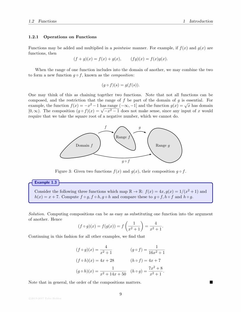
When the range of one function includes into the domain of another, we may combine the twoto form a new function g ◦ f , known as the composition:
(g ◦ f)(s) = g(f(s)).
One may think of this as chaining together two functions. Note that not all functions can becomposed, and the restriction that the range of f be part of the domain of g is essential. Forexample, the function f(x) = −x2−1 has range (−∞,−1] and the function g(x) =
√x has domain
[0,∞). The composition (g ◦ f)(x) =√−x2 − 1 does not make sense, since any input of x would
require that we take the square root of a negative number, which we cannot do.
Domain f
Range f
Range g
f g
g ◦ f
Figure 3: Given two functions f(x) and g(x), their composition g ◦ f .
Example 1.3
Consider the following three functions which map R→ R: f(x) = 4x, g(x) = 1/(x2 + 1) andh(x) = x+ 7. Compute f ◦ g, f ◦ h, g ◦ h and compare these to g ◦ f, h ◦ f and h ◦ g.
Solution. Computing compositions can be as easy as substituting one function into the argumentof another. Hence
(f ◦ g)(x) = f(g(x)) = f
(1
x2 + 1
)=
4
x2 + 1.
Continuing in this fashion for all other examples, we find that
(f ◦ g)(x) =4
x2 + 1(g ◦ f) =
1
16x2 + 1
(f ◦ h)(x) = 4x+ 28 (h ◦ f) = 4x+ 7
(g ◦ h)(x) =1
x2 + 14x+ 50(h ◦ g) =
7x2 + 8
x2 + 1.
Note that in general, the order of the compositions matters. �
c©2013-2017 Tyler Holden
9
1 Introduction 1.2 Functions
1.2.2 Symmetries
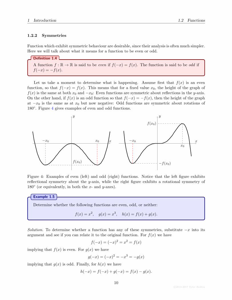
Function which exhibit symmetric behaviour are desirable, since their analysis is often much simpler.Here we will talk about what it means for a function to be even or odd.
Definition 1.4
A function f : R → R is said to be even if f(−x) = f(x). The function is said to be odd iff(−x) = −f(x).
Let us take a moment to determine what is happening. Assume first that f(x) is an evenfunction, so that f(−x) = f(x). This means that for a fixed value x0, the height of the graph off(x) is the same at both x0 and −x0: Even functions are symmetric about reflections in the y-axis.On the other hand, if f(x) is an odd function so that f(−x) = −f(x), then the height of the graphat −x0 is the same as at x0 but now negative: Odd functions are symmetric about rotations of180◦. Figure 4 gives examples of even and odd functions.
x
y
−x0
f(x0)
x0 x
y
−x0
−f(x0)
x0
f(x0)
Figure 4: Examples of even (left) and odd (right) functions. Notice that the left figure exhibitsreflectional symmetry about the y-axis, while the right figure exhibits a rotational symmetry of180◦ (or equivalently, in both the x- and y-axes).
Example 1.5
Determine whether the following functions are even, odd, or neither:
f(x) = x2, g(x) = x3, h(x) = f(x) + g(x).
Solution. To determine whether a function has any of these symmetries, substitute −x into itsargument and see if you can relate it to the original function. For f(x) we have
f(−x) = (−x)2 = x2 = f(x)
implying that f(x) is even. For g(x) we have
g(−x) = (−x)2 = −x3 = −g(x)
implying that g(x) is odd. Finally, for h(x) we have
h(−x) = f(−x) + g(−x) = f(x)− g(x).
10c©2013-2017 Tyler Holden
1.2 Functions 1 Introduction
However, there is no natural way to relate f − g to f + g by using only a single minus sign. Henceh(x) is neither even nor odd. �
1.2.3 Roots
Mathematically, the number 0 is one of the most interesting (and troublesome) numbers. Thestudent is likely familiar with the fact that 0 × a = 0 and 0 + a = a for any value of a, and thatdivision by 0 is strictly prohibited. Hence it is unsurprising that we are often interested in theplaces where functions f : R→ R attain the value 0.
Definition 1.6
Let f : R→ R be a function. We say that α ∈ R is a root of f(x) if f(α) = 0.
Geometrically, roots correspond to the places at which the graph of a function passes throughthe x-axis.
Example 1.7
Find the roots of the functions
f1(x) = x− 5, f2(x) = 0, f3(x) =1
x.
Solution. We begin by looking at f1(x). We want to find values α for which f1(α) = α − 5 = 0.We may simply solve this equation for α to find that α = 5. This is the only possible root of f1(x).It is easy to see that given any function of the form g(x) = x− r, the root of g(x) will be r.
For f2(x), we want the collection of α satisfying f2(α) = 0. Since f2 is just the function whichsends everything to zero, it turns out that every real number is a root of f2(x). This turns out tobe clear when we realize that the graph of f2(x) is just the x-axis itself.
Finally, for f3(x) we want α such that f3(α) = 1/α = 0. In order to solve this equation forα, we would need to take a reciprocal of both sides, but this would require us to divide by zero!Hence 1/α = 0 has no solutions, implying that f3(x) has not roots. Again, try plotting f3(x) andthis will become obvious. �
1.2.4 Piecewise Functions
Piecewise functions are described by gluing together two functions to form a new one. For example,if g(x) and h(x) are two functions and a ∈ R, we may define
f(x) =
{g(x) x ≤ ah(x) x > a
.
This means that if x ≤ a then f(x) = g(x) and if x > a then f(x) = h(x).
c©2013-2017 Tyler Holden
11
1 Introduction 1.2 Functions
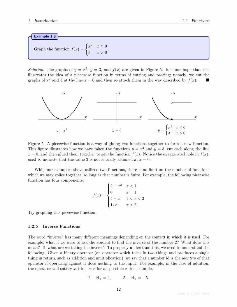
Example 1.8
Graph the function f(x) =
{x2 x ≤ 0
3 x > 0.
Solution. The graphs of y = x2, y = 3, and f(x) are given in Figure 5. It is our hope that thisillustrates the idea of a piecewise function in terms of cutting and pasting; namely, we cut thegraphs of x2 and 3 at the line x = 0 and then re-attach them in the way described by f(x). �
x
y
y = x2
x
y
y = 3
x
y
y =
{x2 x ≤ 0
3 x > 0
Figure 5: A piecewise function is a way of gluing two functions together to form a new function.This figure illustrates how we have taken the functions y = x2 and y = 3, cut each along the linex = 0, and then glued them together to get the function f(x). Notice the exaggerated hole in f(x),used to indicate that the value 3 is not actually attained at x = 0.
While our examples above utilized two functions, there is no limit on the number of functionswhich we may splice together, so long as that number is finite. For example, the following piecewisefunction has four components:
f(x) =
2− x2 x < 1
0 x = 1
4− x 1 < x < 2
1/x x > 2.
Try graphing this piecewise function.
1.2.5 Inverse Functions
The word “inverse” has many different meanings depending on the context in which it is used. Forexample, what if we were to ask the student to find the inverse of the number 2? What does thismean? To what are we taking the inverse? To properly understand this, we need to understand thefollowing: Given a binary operator (an operator which takes in two things and produces a singlething in return, such as addition and multiplication), we say that a number id is the identity of thatoperator if operating against it does nothing to the input. For example, in the case of addition,the operator will satisfy x+ id+ = x for all possible x; for example,
2 + id+ = 2, −5 + id+ = −5.
12c©2013-2017 Tyler Holden
1.2 Functions 1 Introduction
Our experience tells us that id+ = 0. Similarly, for multiplication the identity id× will satisfyx× id× = x for all x; for example,
3× id× = 3, π × id× = π.
Again our experience tells us that id× = 1. We thus say that 0 is the additive identity and 1 is themultiplicative identity. We say that the inverse of x is an element which, when paired against x,gives the identity. Hence the additive inverse of 2 is the number y such that 2 + y = id+ = 0, orrather −2. In general, the additive inverse of n is −n, and this always exists! For multiplication,it is not too hard to convince ourselves that the multiplicative inverse of x is 1
x ; for example,2× 1
2 = 1 = id×. Notice that there is no multiplicative inverse for the number 0, so in this case theinverse does not always exist.
Function composition f ◦ g is another example of a binary operator. What is the identity forthis operation? Well, we would like a function id◦ such that
f(id◦(x)) = f(x)
= id◦(f(x)).
If we this about this for a moment, the identity function is the function id◦(x) = x, the functionwhich does nothing to the argument! Now what is the inverse of a function? The inverse of afunction f(x) is a function f−1(x) such that f ◦ f−1 = f−1 ◦ f = id◦.
To compute the inverse of y = f(x), notice that by applying f−1 to both sides we get
f−1(y) = f−1(f(x)) = x.
Hence by switching x and y and solving for y, we get y = f−1(x).
Example 1.9
Determine the inverse of the function y = f(x) = (x− 1)/(x+ 1).
Solution. As recommended above, we interchange y and x and solve for y, so we get
x =y − 1
y + 1⇔ (y + 1)x = y − 1
⇔ yx− y = −(x+ 1)
⇔ y(x− 1) = −(x+ 1)
⇔ y =x+ 1
1− xSo f−1(x) = (x + 1)/(1 − x). Indeed we can check this by composing f ◦ f−1 and f−1 ◦ f to findthat
f(f−1(x)) =x+11−x − 1x+11−x + 1
=x+1−1−x
1−xx+1+1−x
1−x=
2x
2
= x
and the other direction is left as an exercise. �
c©2013-2017 Tyler Holden
13
1 Introduction 1.3 Polynomials and Rational Functions
Note that not all functions are invertible. For example, the function f(x) = x2 is not invertiblein general. It is tempting to say that g(x) =
√x is the inverse to f , but this is not the case. Indeed,
while we do have that(f ◦ g) =
(√x)2
= x,
the opposite composition gives(g ◦ f)(x) =
√x2 = |x|
which is not the identity function. To test whether a function can be inverted, it must satisfy thehorizontal line test ; that is, every horizontal line must intersect the graph of f in at most one place.
Exercise
Determine the inverses of each of the following functions. What special property do f, g, andh all share?
f(x) =1
x, g(x) = 1− x, h(x) =
x
x− 1.
1.3 Polynomials and Rational Functions
Polynomials are the collection of all objects of the form
anxn + an−1x
n−1 + · · ·+ a2x2 + a1x+ a0
for some natural number n > 0 and real numbers a0, a1, . . . , an. We say that the degree of apolynomial is the highest power whose coefficient is non-zero. For example, the following functionsare polynomials
p(x) = 3x4 + 8x3 − 2x, q(x) = 39x66 − 5x2 + 1
and the degree of p(x) is 4 while the degree of q(x) is 66. Some degrees occur so frequently thatthey even have special names:
Degree Name
1 Linear2 Quadratic3 Cubic4 Quartic5 Quintic
Factoring polynomials is the process by which we reverse the act of multiplying a polynomial:We would like to write a single polynomial as a product of polynomials with strictly smaller degree.
There are some very easy factorization which involve simply removing a power of x. If there isno constant term (the coefficient of x0 is 0), then we may remove at least one power of x from thepolynomial. For example,
x4 + x2 = x2(x2 + 1), x5 + x4 + x = x(x4 + x3 + 1).
In general, factoring polynomials with constant terms can be incredibly difficult. For most purposeshowever, we may limit ourselves to factoring quadratic polynomials. Given a quadratic polynomial
14c©2013-2017 Tyler Holden
1.4 Absolute Values 1 Introduction
of the form x2 +ax+ b, the trick is to try and find two numbers p, q such that a = p+ q and b = pq.This is because
(x+ p)(x+ q) = x2 + (p+ q)x+ pq.
Example 1.10
Factor the following polynomials:
x2 + 2x+ 1, 3x2 + 15x+ 18, x2 − 1, x3 − x2 − 2x.
Solution. We begin with x2 + 2x + 1. To factor this, we try to think of two numbers p, q suchthat p + q = 2 and pq = 1. Hopefully, the choice p = 1, q = 1 springs to our minds and we guess(x+ 1)(x+ 1) = x2 + 2x+ 1. A quick check verifies that this is the case.
For 3x2 + 15x+ 18 we are not quite in the situation described above as the coefficient in frontof x2 is not 1. However, we may first factor out a 3 to get 3x2 + 15x+ 18 = 3(x2 + 5x+ 6). Nowwe would like to find p, q such that p + q = 5 and pq = 6. The choice p = 2 and q = 3 jumps tomind, and a quick calculation verifies that (x+ 2)(x+ 3) = x2 + 5x+ 6. Thus
3x2 + 15x+ 18 = 3(x+ 2)(x+ 3).
The polynomial x2 − 1 look tricky: what do we do if we have no x term? Instead of panicking,let’s try our usual technique; that is, find p, q such that p + q = 0 and pq = −1. We couldactually solve this equation, or just guess that p = 1 and q = −1 work. Indeed, it turns out thatx2 − 1 = (x+ 1)(x− 1).
Finally, x3−x2−2x is not a quadratic polynomial. However, the lack of a constant term meanswe can first factor out an x term to get x3 − x2 − 2x = x(x2 − x− 2). We hence content ourselvesto find p, q such that p + q = −1 and pq = −2. This one is a bit tricky, but some though revealsthat p = −2 and q = 1 will do the trick, and indeed (x− 2)(x+ 1) = x2 − x− 2 so that
x3 − x2 − 2x = x(x− 2)(x+ 1). �
Rational functions are quotients of polynomials; that is, they are functions which can be writtenas f(x) = p(x)/q(x) where p(x) and q(x) are both polynomials. The following are examples ofrational functions:
f(x) =x2 + 2x+ 1
x− 1, g(x) =
1
x2 + 1, h(x) =
x3 + 2x− 1
4x4 − x2 + 13.
1.4 Absolute Values
One of the most important concepts in mathematics is that of length, historically motivated byapplications and the Greek obsession with compasses and rulers. One finds that there are a hierarchyof structures, each more powerful than the next, that endow a space with a measure of length:metrics, norms, and inner products.
We shall not study such structures in this course, but the student who ventures into the studyof linear algebra will quickly find him/herself acquainted with norms and inner products.
c©2013-2017 Tyler Holden
15
1 Introduction 1.4 Absolute Values
1.4.1 The Absolute Value
Given a number x ∈ R we would like to discuss its “distance” from the number 0. Naively, wewould like to say something along the lines of “4 is the same distance from 0 as −4” or perhaps “2is the same distance from 4 as −1 is from −3.” Figure 6 illustrates this idea.
−5 0 5
Figure 6: The real line from −5 to positive 5. We would like to define a system of measurementsuch that the red bars have the same length and the blue bars have the same length.
The formal way to talk about the concept of length is with absolute values:
Definition 1.11
For x ∈ R we define the absolute value of x as
|x| ={
x x ≥ 0−x x < 0
.
Notice that the absolute value is always positive: If x is already positive, the absolute valuedoes not do anything, while if x is negative we negate it again to make it positive. Geometrically,we may interpret |x| as the distance from x to 0. The distance from 4 to 0 is |4| = 4 while thedistance from −4 to 0 is | − 4| = −(−4) = 4. As we discussed above, this is precisely what weexpected.
Proposition 1.12: Properties of the Absolute Value
If a, b ∈ R then1. |ab| = |a||b| (Multiplicative)2. |a+ b| ≤ |a|+ |b| (Triangle Inequality)3. |a| = 0 if and only if a = 0 (Non-degenerate).
1.4.2 Relation to Intervals
Instead of looking at the distance from a to 0, we can look at the distance between a and b, givenby |a− b|. Therefore, we may use absolute values combined with inequalities to describe intervals.For example, consider the statement |x− c| < a. Using the definition of the absolute value, we canwrite this as
|x− c| ={x− c x ≥ cc− x x < c
.
Now |x − c| < a implies that both x − c < a and c − x < a for all values of x. If we multiplyc− x < a by −1 we get x− c > −a, which we may combine with x− c < a to conclude that
|x− c| < a ⇐⇒ −a < x− c < a.
We may read |x− c| < a geometrically as
16c©2013-2017 Tyler Holden
1.4 Absolute Values 1 Introduction
“The distance from x to c is less than a.”
Intuitively, the set of all x which satisfy this will lie in the interval (c− a, c+ a). We can show thismore concretely by realizing that
|x− c| < a ⇐⇒ −a < x− c < a
⇐⇒ c− a < x < c+ a(1.1)
Example 1.13
Find the intervals corresponding to all x which satisfy the following inequalities:
|x| ≤ 1, |2x− 5| < 3, |x+ 7| > 5.
Solution. If |x| ≤ 1 then −1 ≤ x ≤ 1 and this corresponds to the interval [−1, 1]. The next exampleis |x− 2| < 3 and proceeding by the same argument in (1.1) we find that
|2x− 5| < 3 ⇐⇒ −3 < 2x− 5 < 3
⇐⇒ 2 < 2x < 8
⇐⇒ 1 < x < 4
so that the corresponding interval is (1, 4).
Expressions of the form |x+ 7| > 5 will occur far less frequently than the examples consideredabove, but should still be solvable if we go back to the definition of absolute value. Intuitively we seethat the x which satisfy this will be a distance of at least 5 from −7; that is, (−∞,−12)∪ (−2,∞).Let us check that this is the case.
The condition that |x+ 7| > 5 implies that both x+ 7 > 5 and −x− 7 > 5. Solving the formerfor x we find that x > −2 while the latter reveals that x < −12, precisely as we expected. �
1.4.3 Algebra with Inequalities
Students often have troubles with absolute values, especially when encountering them while solvingfor a variable. Whenever absolute values are encountered, the best strategy in each case is toremove the absolute values by considering cases in which the absolute values can be removed.
Example 1.14
Find all x for which |x+ 7| < 4x+ 10.
Solution. The equation |x + 7| < 4x + 10 is untenable in this form, so we break it into the casex < −7 where |x+ 7| = −x− 7 and x ≥ −7 where |x+ 7| = x+ 7.
Case x < −7: If we restrict ourselves to x < −7 then |x+ 7| < 4x+ 10 becomes
−x− 7 < 4x+ 10.
c©2013-2017 Tyler Holden
17
1 Introduction 1.4 Absolute Values
Some quick algebraic manipulation shows us that x > −175 , which combined with x < −7 tells us
that no x satisfy this equation.
Case x ≥ −7: In this case |x+ 7| < 4x+ 10 becomes x+ 7 < 4x+ 10. Some algebraic work showsus that x > −1. Hence both x > −1 and x ≥ −7 implies that x > −1 is the solution.
Combining the results from both cases, we see that |x + 7| < 4x + 10 if x > −1; that is,x ∈ (−1,∞). �
Example 1.15
Find all x for which|x− 3| ≥ |x+ 1| − 2. (1.2)
Solution. The expression |x−3| will change signs at x = 3 while |x+1| will switch signs at x = −1.This implies that we should consider three cases: x < −1, −1 < x < 3, and x > 3.
Case x < −1: Equation (1.2) becomes
−x+ 3 ≥ −x− 1− 2.
The x’s will actually cancel giving the expression 3 ≥ −3, which is clearly true, so x < −1 alwayssatisfies the equation.
Case −1 < x < 3: In this case equation (1.2) becomes
−x+ 3 ≥ x+ 1− 2
which is solved to find x ≤ 2. Hence x must satisfy both −1 < x < 3 and x ≤ 2 implying that−1 < x ≤ 2.
Case x > 3: Now equation (1.2) becomes
x− 3 ≥ x+ 1− 2
which yields −3 ≥ −1, a false expression. This means that no x in this region satisfies the equation.
Finally, we check the switch points x = −1, 3 themselves. Substituting x = −1 into (1.2) weget
|(−1) + 3| ≥ |(−1) + 1|+ 2 ⇒ 2 ≥ 2
which is true, so that −1 satisfies the equation. On the other hand, x = 3 yields
|3− 3| ≥ |3 + 1|+ 2 ⇒ 0 ≥ 6
which is not true, so x = 2 does not satisfy the equation. Combining all of our information, thetotal solution is
{x < −1} ∪ {−1 < x ≤ 2} ∪ {−1} = {x ≤ 2}
or more concisely, the interval (−∞, 2] �
18c©2013-2017 Tyler Holden
1.5 Trigonometric Functions 1 Introduction
1.5 Trigonometric Functions
Trigonometry seems to be ubiquitously alluded to as the bane of every secondary school student,but it should not be feared. A solid foundation and understanding of some simple trigonometrywill be essential for the study of calculus as well as crucial for many applications in industry.
In case the student is unfamiliar, we recall that trigonometric functions arise in the study ofangles, and in particular we typically associate them with triangles.
1.5.1 Degrees versus radians
When one is first introduced to angles, one typically learns that we measure them in degrees;namely, we say that a full rotation of a circle is equal to 360◦ and then divide the circle into 360equal portions. The angle made by each of these portions is a single degree.
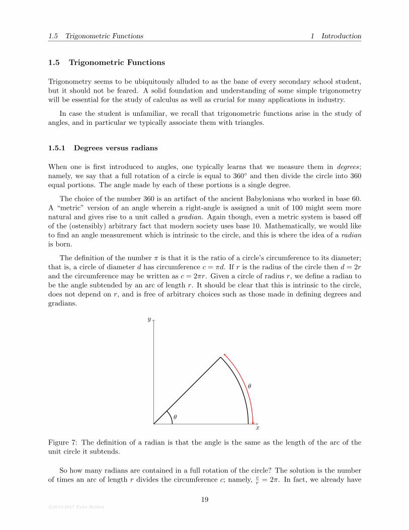
The choice of the number 360 is an artifact of the ancient Babylonians who worked in base 60.A “metric” version of an angle wherein a right-angle is assigned a unit of 100 might seem morenatural and gives rise to a unit called a gradian. Again though, even a metric system is based offof the (ostensibly) arbitrary fact that modern society uses base 10. Mathematically, we would liketo find an angle measurement which is intrinsic to the circle, and this is where the idea of a radianis born.
The definition of the number π is that it is the ratio of a circle’s circumference to its diameter;that is, a circle of diameter d has circumference c = πd. If r is the radius of the circle then d = 2rand the circumference may be written as c = 2πr. Given a circle of radius r, we define a radian tobe the angle subtended by an arc of length r. It should be clear that this is intrinsic to the circle,does not depend on r, and is free of arbitrary choices such as those made in defining degrees andgradians.
x
y
θ
θ
Figure 7: The definition of a radian is that the angle is the same as the length of the arc of theunit circle it subtends.
So how many radians are contained in a full rotation of the circle? The solution is the numberof times an arc of length r divides the circumference c; namely, c
r = 2π. In fact, we already have
c©2013-2017 Tyler Holden
19
1 Introduction 1.5 Trigonometric Functions
enough tools to discuss the length of a circular sector.
Proposition 1.16
Consider a circle of radius r and a circular sector subtended by an angle of θ. The outerperimeter s of the sector is given by the formula s = rθ.
Proof. The idea is as follows: we know that the sector given by an angle to 2π is the whole circle,giving a sector length of c = 2πr. If 0 < θ < 2π then the sector subtended by the angle θ will havea sector length equal to the ratio of θ to the whole circle, 2π. Hence
s =2πr2πθ
= 2πrθ
2π= rθ.
It is essential at this point to remark that the usual formulas derived and used in the studyof calculus assume the use of radians. The wayward student who attempts to use the theoryof calculus to make computations, but substitutes degrees instead of radians, may find themselvessending lunar rockets to the sun instead of the moon. As such, it is necessary to discuss theconversion between radians and degrees.
There are π radians for every 180 degrees, so we may convert between the two via the followingformulas:
degrees =180
π× radians, radians =
π
180× degrees.
These formulas are easy to remember if the student thinks about “canceling” the units, demon-strated in the following example.
Example 1.17
Convert π3 radians to degrees, and 45◦ to radians.
Solution. We use our formula to compute the conversions. We have
degrees =180 degrees
π ����radians× π
3����radians
=180
3degrees
= 60 degrees.
Similarly converting from degrees to radians we have
radians =π radians
180 ����degrees× 45 ����degrees
=45π
180radians
=π
4radians. �
20c©2013-2017 Tyler Holden
1.5 Trigonometric Functions 1 Introduction
1.5.2 Trigonometric Functions
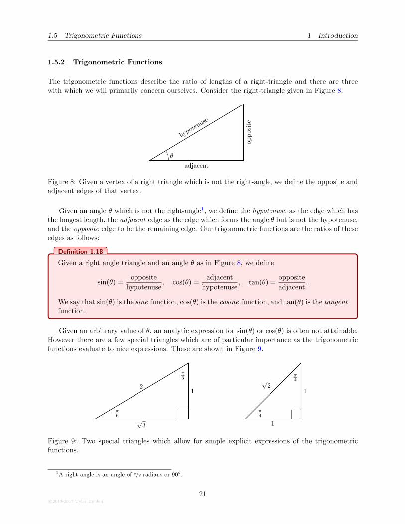
The trigonometric functions describe the ratio of lengths of a right-triangle and there are threewith which we will primarily concern ourselves. Consider the right-triangle given in Figure 8:
adjacent
opposite
hypoten
use
θ
Figure 8: Given a vertex of a right triangle which is not the right-angle, we define the opposite andadjacent edges of that vertex.
Given an angle θ which is not the right-angle1, we define the hypotenuse as the edge which hasthe longest length, the adjacent edge as the edge which forms the angle θ but is not the hypotenuse,and the opposite edge to be the remaining edge. Our trigonometric functions are the ratios of theseedges as follows:
Definition 1.18
Given a right angle triangle and an angle θ as in Figure 8, we define
sin(θ) =opposite
hypotenuse, cos(θ) =
adjacent
hypotenuse, tan(θ) =
opposite
adjacent.
We say that sin(θ) is the sine function, cos(θ) is the cosine function, and tan(θ) is the tangentfunction.
Given an arbitrary value of θ, an analytic expression for sin(θ) or cos(θ) is often not attainable.However there are a few special triangles which are of particular importance as the trigonometricfunctions evaluate to nice expressions. These are shown in Figure 9.
√3
12
π6
π3
1
1
√2
π4
π4
Figure 9: Two special triangles which allow for simple explicit expressions of the trigonometricfunctions.
1A right angle is an angle of π/2 radians or 90◦.
c©2013-2017 Tyler Holden
21
1 Introduction 1.5 Trigonometric Functions
Example 1.19
Find the values of sin(π3
)and cos
(π4
).
Solution. Using Definition 1.18 and the special triangles shown in Figure 9, we can easily read off
sin(π
3
)=
√3
2, cos
(π4
)=
1√2. �
1.5.3 Between circles and triangles
It was mentioned in the beginning of this section that we associate trigonometric functions withtriangles, while our discussion concerning radians concerns circles. What is the relationship betweenthem?
The circle, despite being drawn in the two-dimensional plane, is really only a one dimensionalobject. Indeed, if you lived on a circle you could only move forwards or backwards, hence onedimension. This means that mathematically we should be able to write points on the circle interms of a single parameter.
Our goal is to write a point (x, y) on the unit circle purely in terms of the angle θ made by thepositive x-axis and the line connecting (x, y) to the origin. If the radius of the circle is r, Definition1.18 tells us that x = r cos(θ) and y = r sin(θ). The Pythagorean theorem says that x2 + y2 = r2,so in turn we have the identity2
r2 sin2(θ) + r2 cos2(θ) = r2.
As r 6= 0 we may divide through to get the Pythagorean trigonometric identity
sin2(θ) + cos2(θ) = 1. (1.3)
This equation can be seen directly by setting the radius of the circle to be r = 1 and is shown inFigure 10.
Measuring angles on the circle gives us a useful technique for determining the sign of a trigono-metric function. For example, consider the values
sin(π
6
), sin
(5π
6
), sin
(7π
6
), sin
(11π
6
).
Figure 11 shows the angles as inscribed in a circle. The hypotenuse (corresponding to the radiusof the circle) is the same for each triangle drawn, and the length of the opposite angle is also thesame. However, notice that in the quadrants I and II the opposite length (corresponding to the
2The notation sin2(x) can be confusing, but this is how the expression (sin(x))2 is always denoted; that is,sin2(x) = sin(x) sin(x). To exacerbate matters, many authors use f2(x) to denote the two-fold composition f(f(x)),but this is not what is meant with trigonometric functions.
22c©2013-2017 Tyler Holden
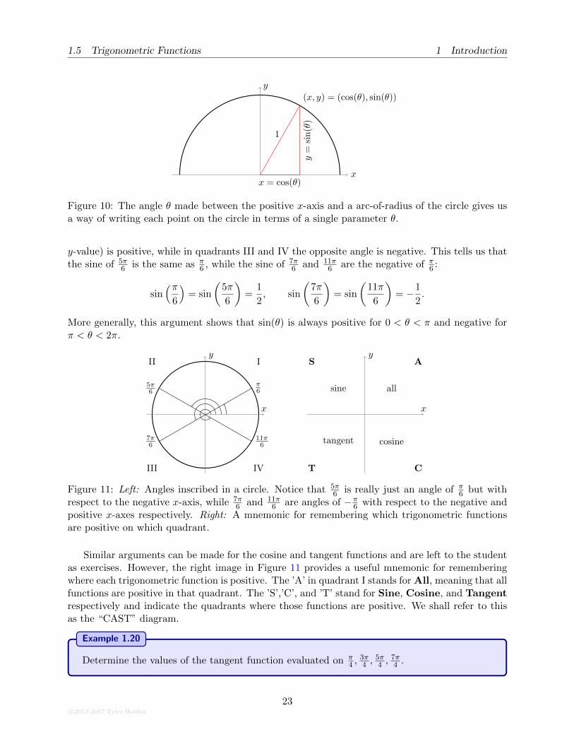
1.5 Trigonometric Functions 1 Introduction
x
y
x = cos(θ)
y=
sin(θ)
(x, y) = (cos(θ), sin(θ))
1
Figure 10: The angle θ made between the positive x-axis and a arc-of-radius of the circle gives usa way of writing each point on the circle in terms of a single parameter θ.
y-value) is positive, while in quadrants III and IV the opposite angle is negative. This tells us thatthe sine of 5π
6 is the same as π6 , while the sine of 7π
6 and 11π6 are the negative of π
6 :
sin(π
6
)= sin
(5π
6
)=
1
2, sin
(7π
6
)= sin
(11π
6
)= −1
2.
More generally, this argument shows that sin(θ) is always positive for 0 < θ < π and negative forπ < θ < 2π.
x
y
7π6
π6
5π6
11π6
III
III IV
x
y
allsine
tangent cosine
AS
T C
Figure 11: Left: Angles inscribed in a circle. Notice that 5π6 is really just an angle of π
6 but withrespect to the negative x-axis, while 7π
6 and 11π6 are angles of −π
6 with respect to the negative andpositive x-axes respectively. Right: A mnemonic for remembering which trigonometric functionsare positive on which quadrant.
Similar arguments can be made for the cosine and tangent functions and are left to the studentas exercises. However, the right image in Figure 11 provides a useful mnemonic for rememberingwhere each trigonometric function is positive. The ’A’ in quadrant I stands for All, meaning that allfunctions are positive in that quadrant. The ’S’,’C’, and ’T’ stand for Sine, Cosine, and Tangentrespectively and indicate the quadrants where those functions are positive. We shall refer to thisas the “CAST” diagram.
Example 1.20
Determine the values of the tangent function evaluated on π4 ,
3π4 ,
5π4 ,
7π4 .
c©2013-2017 Tyler Holden
23
1 Introduction 1.5 Trigonometric Functions
Solution. The angle π4 refers to one of the special triangles, so we immediately gauge that tan
(π4
)=
1. To determine the other three angles we refer to Figure 11. The figure tells us that the tangentfunction is positive in quadrants I and III and negative everywhere else indicated that
tan(π
4
)= tan
(5π
4
)= 1, tan
(3π
4
)= tan
(7π
4
)= −1. �
1.5.4 The Reciprocal Trigonometric Functions
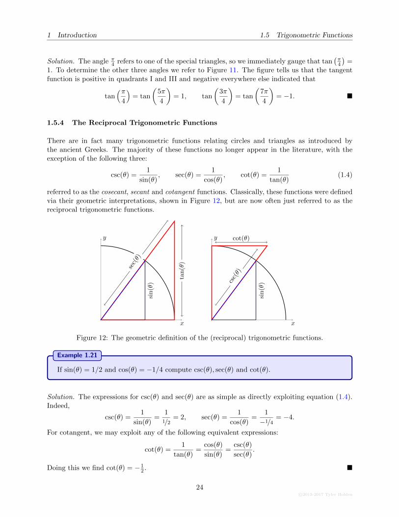
There are in fact many trigonometric functions relating circles and triangles as introduced bythe ancient Greeks. The majority of these functions no longer appear in the literature, with theexception of the following three:
csc(θ) =1
sin(θ), sec(θ) =
1
cos(θ), cot(θ) =
1
tan(θ)(1.4)
referred to as the cosecant, secant and cotangent functions. Classically, these functions were definedvia their geometric interpretations, shown in Figure 12, but are now often just referred to as thereciprocal trigonometric functions.
x
y
sin(θ)
tan(θ)
sec(θ)
x
y
sin(θ)csc(θ)
cot(θ)
Figure 12: The geometric definition of the (reciprocal) trigonometric functions.
Example 1.21
If sin(θ) = 1/2 and cos(θ) = −1/4 compute csc(θ), sec(θ) and cot(θ).
Solution. The expressions for csc(θ) and sec(θ) are as simple as directly exploiting equation (1.4).Indeed,
csc(θ) =1
sin(θ)=
11/2
= 2, sec(θ) =1
cos(θ)=
1
−1/4= −4.
For cotangent, we may exploit any of the following equivalent expressions:
cot(θ) =1
tan(θ)=
cos(θ)
sin(θ)=
csc(θ)
sec(θ).
Doing this we find cot(θ) = −12 . �
24c©2013-2017 Tyler Holden
1.5 Trigonometric Functions 1 Introduction
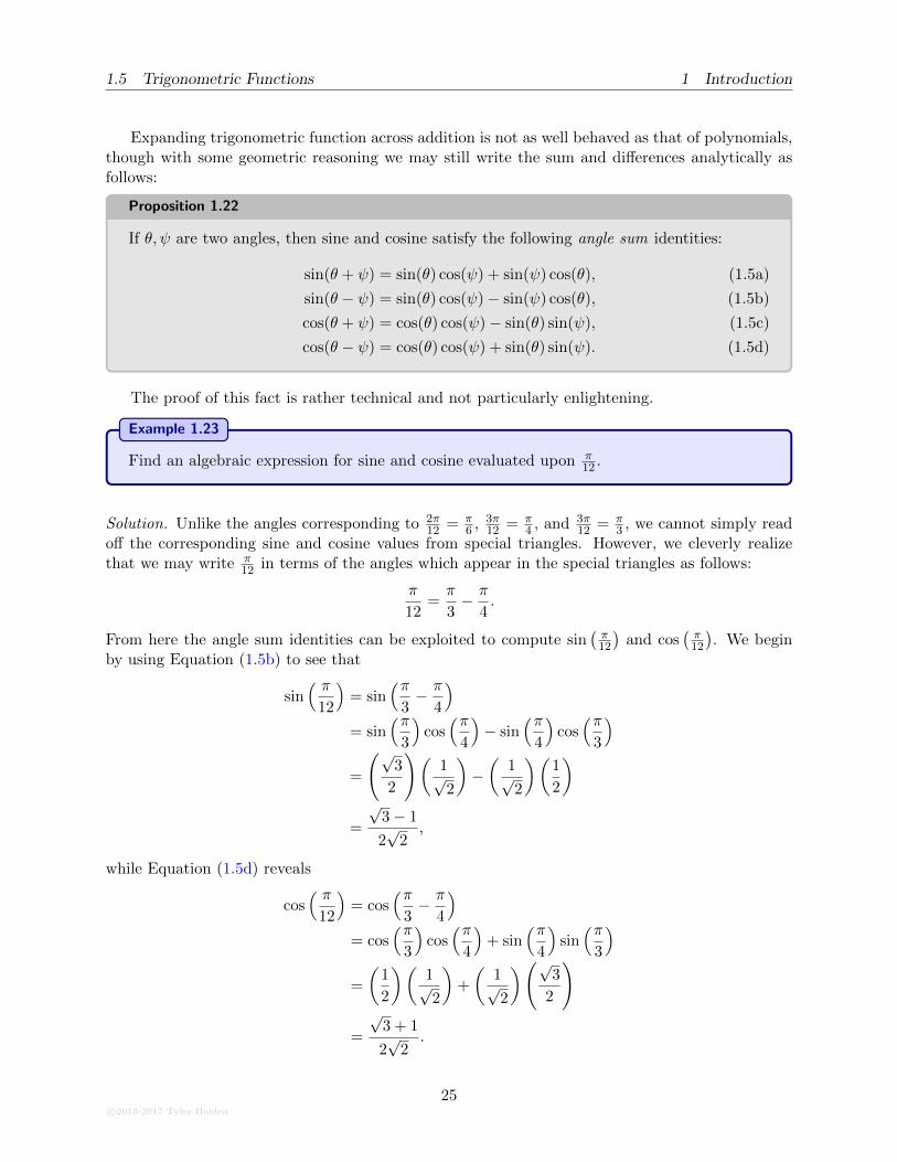
Expanding trigonometric function across addition is not as well behaved as that of polynomials,though with some geometric reasoning we may still write the sum and differences analytically asfollows:
Proposition 1.22
If θ, ψ are two angles, then sine and cosine satisfy the following angle sum identities:
sin(θ + ψ) = sin(θ) cos(ψ) + sin(ψ) cos(θ), (1.5a)
sin(θ − ψ) = sin(θ) cos(ψ)− sin(ψ) cos(θ), (1.5b)
cos(θ + ψ) = cos(θ) cos(ψ)− sin(θ) sin(ψ), (1.5c)
cos(θ − ψ) = cos(θ) cos(ψ) + sin(θ) sin(ψ). (1.5d)
The proof of this fact is rather technical and not particularly enlightening.
Example 1.23
Find an algebraic expression for sine and cosine evaluated upon π12 .
Solution. Unlike the angles corresponding to 2π12 = π
6 , 3π12 = π
4 , and 3π12 = π
3 , we cannot simply readoff the corresponding sine and cosine values from special triangles. However, we cleverly realizethat we may write π
12 in terms of the angles which appear in the special triangles as follows:
π
12=π
3− π
4.
From here the angle sum identities can be exploited to compute sin(π12
)and cos
(π12
). We begin
by using Equation (1.5b) to see that
sin( π
12
)= sin
(π3− π
4
)
= sin(π
3
)cos(π
4
)− sin
(π4
)cos(π
3
)
=
(√3
2
)(1√2
)−(
1√2
)(1
2
)
=
√3− 1
2√
2,
while Equation (1.5d) reveals
cos( π
12
)= cos
(π3− π
4
)
= cos(π
3
)cos(π
4
)+ sin
(π4
)sin(π
3
)
=
(1
2
)(1√2
)+
(1√2
)(√3
2
)
=
√3 + 1
2√
2.
c©2013-2017 Tyler Holden
25
1 Introduction 1.6 Exponential Functions
These expression are exact, but are rather unwieldy to work with and might have been hard todeduce without the angle sum identities. �
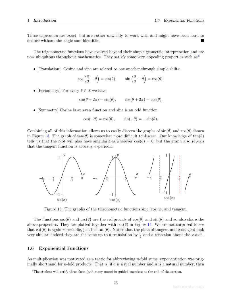
The trigonometric functions have evolved beyond their simple geometric interpretation and arenow ubiquitous throughout mathematics. They satisfy some very appealing properties such as3:
• [Translation:] Cosine and sine are related to one another through simple shifts:
cos(π
2− θ)
= sin(θ), sin(π
2− θ)
= cos(θ).
• [Periodicity:] For every θ ∈ R we have
sin(θ + 2π) = sin(θ), cos(θ + 2π) = cos(θ).
• [Symmetry] Cosine is an even function and sine is an odd function:
cos(−θ) = cos(θ), sin(−θ) = − sin(θ).
Combining all of this information allows us to easily discern the graphs of sin(θ) and cos(θ) shownin Figure 13. The graph of tan(θ) is somewhat more difficult to discern. Our knowledge of tan(θ)tells us that the plot will also have singularities wherever cos(θ) = 0, but the graph also revealsthat the tangent function is actually π-periodic.
x
y
−π −π2
π2
π
−1
1
sin(x)
x
y
−π −π2
π2
π
cos(x)
−1
1
−π −π2
π2
π
−1
1
tan(x)
Figure 13: The graphs of the trigonometric functions sine, cosine, and tangent.
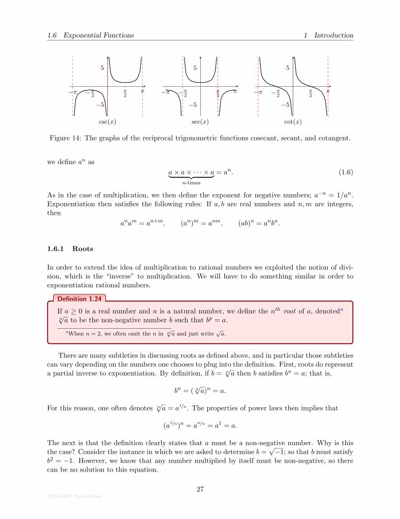
The functions sec(θ) and csc(θ) are the reciprocals of cos(θ) and sin(θ) and so also share theabove properties. They are plotted together with cot(θ) in Figure 14. We are not surprised to seethat cot(θ) is again π-periodic, just like tan(θ). Notice that the plots of tangent and cotangent lookvery similar: indeed they are the same up to a translation by π
2 and a reflection about the x-axis.
1.6 Exponential Functions
As multiplication was motivated as a tactic for abbreviating n-fold sums, exponentiation was orig-inally shorthand for n-fold products. That is, if a is a real number and n is a natural number, then
3The student will verify these facts (and many more) in guided exercises at the end of the section.
26c©2013-2017 Tyler Holden
1.6 Exponential Functions 1 Introduction
−π −π2
π2
π
−5
5
csc(x)
−π −π2
π2
π
−5
5
sec(x)
−π −π2
π2
π
−5
5
cot(x)
Figure 14: The graphs of the reciprocal trigonometric functions cosecant, secant, and cotangent.
we define an as
a× a× · · · × a︸ ︷︷ ︸n-times
= an. (1.6)
As in the case of multiplication, we then define the exponent for negative numbers; a−n = 1/an.Exponentiation then satisfies the following rules: If a, b are real numbers and n,m are integers,then
anam = an+m, (an)m = anm, (ab)n = anbn.
1.6.1 Roots
In order to extend the idea of multiplication to rational numbers we exploited the notion of divi-sion, which is the “inverse” to multiplication. We will have to do something similar in order toexponentiation rational numbers.
Definition 1.24
If a ≥ 0 is a real number and n is a natural number, we define the nth root of a, denoteda
n√a to be the non-negative number b such that bp = a.
aWhen n = 2, we often omit the n in n√a and just write
√a.
There are many subtleties in discussing roots as defined above, and in particular those subtletiescan vary depending on the numbers one chooses to plug into the definition. First, roots do representa partial inverse to exponentiation. By definition, if b = n
√a then b satisfies bn = a; that is,
bn = ( n√a)n = a.
For this reason, one often denotes n√a = a1/n. The properties of power laws then implies that
(a1/n)n = a
n/n = a1 = a.
The next is that the definition clearly states that a must be a non-negative number. Why is thisthe case? Consider the instance in which we are asked to determine b =
√−1; so that b must satisfy
b2 = −1. However, we know that any number multiplied by itself must be non-negative, so therecan be no solution to this equation.
c©2013-2017 Tyler Holden
27

1 Introduction 1.6 Exponential Functions
Furthermore, if we consider the case b =√
4 we see that there are two numbers satisfying b2 = 4:b = 2 and b = −2. Since we would like roots to define functions we can only choose one b as oursolution, so we establish the convention of always choosing the positive solution.
The problems discussed above were demonstrated in the case when n = 2, and it turns outthat these pathological examples only occur when n is even. When n is odd, there is no issue withtaking nth roots of negative numbers, nor with the existence of multiple solutions. As an example,consider b = 3
√−8. There is a unique number, b = −2, such that b3 = −8. We summarize our
discussion below.
1. If n is even and a ≥ 0, then bn = a will have multiple solutions. To avoid ambiguity indefining n
√a, we demand that b must be non-negative.
2. If n is even, it is impossible to define the nth root of a negative number.
3. If n is odd, then neither 1 nor 2 apply; that is, there is a unique solution to bn = a for anya ∈ R.
Example 1.25
Determine the values of√
9 and 3√−64.
Solution. Starting with√
9, our goal is to find a positive integer b such that b2 = 9. We know thatthere will be multiple solutions since n = 2 is even, and indeed b = 3 and b = −3 both work. Asour definition stipulates that b must be non-negative, we take b = 3 and conclude that
√9 = 3.
On the other hand, as n = 3 is odd we know that b = 3√−64 is the unique solution to b3 = −64.
A bit of trial and error shows that (−4)3 = −64 and so 3√−64 = −4. �
By exploiting the identities given in Equation (1.6), we can immediately deduce the followingfor roots: If a, b ∈ R and m,n ∈ Z then
n√a m√a =
m+nmn√a,
n
√m√a = mn
√a,
n√ab = n
√an√b. (1.7)
1.6.2 Logarithms
Given the equation an = b, we have discussed exponentiation and the process of taking roots. Inessence, these ideas boil down to a two-out-of-three argument; that is, given two of variables solvefor the third. For exponentiation, one is given a and n and told to determine b, while given n andb we may take nth roots to determine a. The remaining situation, given a and b determine n, isdescribed by logarithms.
Why might we want to find such an n? There are many industrial reasons, the most often ofwhich appear in pre-calculus courses as problems in finance. As an example, one is told that anasset appreciates at a fixed rate of 4% per annum and is tasked with determining the number ofyears until the asset’s worth has doubled. This amounts to solving the equation (1.04)b = 2, whichwe see is precisely the aforementioned problem which logarithms are designed to solve.
28c©2013-2017 Tyler Holden
1.6 Exponential Functions 1 Introduction
From a mathematical perspective, logarithms will arise as the inverse function to exponentiation.We saw that for a fixed natural number n we could invert the process of exponentiation xn by takingan nth root. This is useful if we want to talk about inverses of polynomials: if f(x) = x3 thenf−1(x) = 3
√x. If we now fix the base and let the exponent vary, taking roots is very much untenable;
in fact, our goal is to find the exponent itself! Logarithms are the solution to the inversion problem.
an = b
ExponentiationGiven: a and n
Determine: c
RootsGiven: n and b
Determine: a
LogarithmsGiven: a and b
Determine: n
Table 1: A description of the possible “two-out-of-three” situations arising from the equation an = b.
Definition 1.26
If a and b are positive numbers, we define loga b (read as the base-a logarithm of b) as thenumber c satisfying ac = b.
If the student is unfamiliar with logarithms the above definition can be a lot to take in. Wewould encourage the student to take a second and parse Definition 1.26 until it starts to makesense.
Example 1.27
Compute log2 32, log3 27.
Solution. Let c = log2 32 in which case Definition 1.26 implies that c must satisfy 2c = 32. Thestudent will hopefully recall (or easily compute) that 25 = 32, so c = 5 and we conclude thatlog2 32 = 5.
Similarly, if c = log3 27 then 3c = 27. The student can then easily check that 33 = 27 and solog3 27 = 3. �
The manner in which we started this section should suggest that the logarithm is going to playthe inverse role to exponentiation. Indeed, items 3 and 4 in the following proposition shed somelight on the relationship between logarithms and exponentials.
Proposition 1.28: I
a and b are positive real numbers with a 6= 1, then
1. loga(1) = 0
2. loga(a) = 1
3. loga(ab) = b
4. aloga(b) = b
c©2013-2017 Tyler Holden
29
1 Introduction 1.6 Exponential Functions
These results are very simple and, as always, the student should make an attempt to prove theresults on their own before looking at the proof. This will not only build confidence in workingwith logarithms, but also expand the student’s comprehension of the subject.
Proof. 1. Set c = loga(1) so that ac = 1. Since a 6= 1 by hypothesis, it must be the case thatc = 0. Thus loga(1) = 0 as required.
2. Similar to part 1, we know that c = loga(a) satisfies ac = a. It is not to hard to see thatc = 1 is the only possible solution and hence loga(a) = 1.
3. Let c = loga(ab) so that c satisfies ac = ab. It should be clear4 that c = b is the solution, so
that loga(ab) = b.
4. Let c = loga(b) so that ac = b. However, simply substituting our first expression of c into thelatter expression, we get aloga(b) = b as required.
1.6.3 The Exponential and Logarithmic Functions
The procedure for extending exponentiation from an for natural numbers n, to ax for real numbersx, is quite difficult. It requires that we either have access to the mathematics of sequences (whichwe will not cover), or integration (which is not covered until the second half of the course). As aresult, the student is going to have to take my word that such extensions exist.
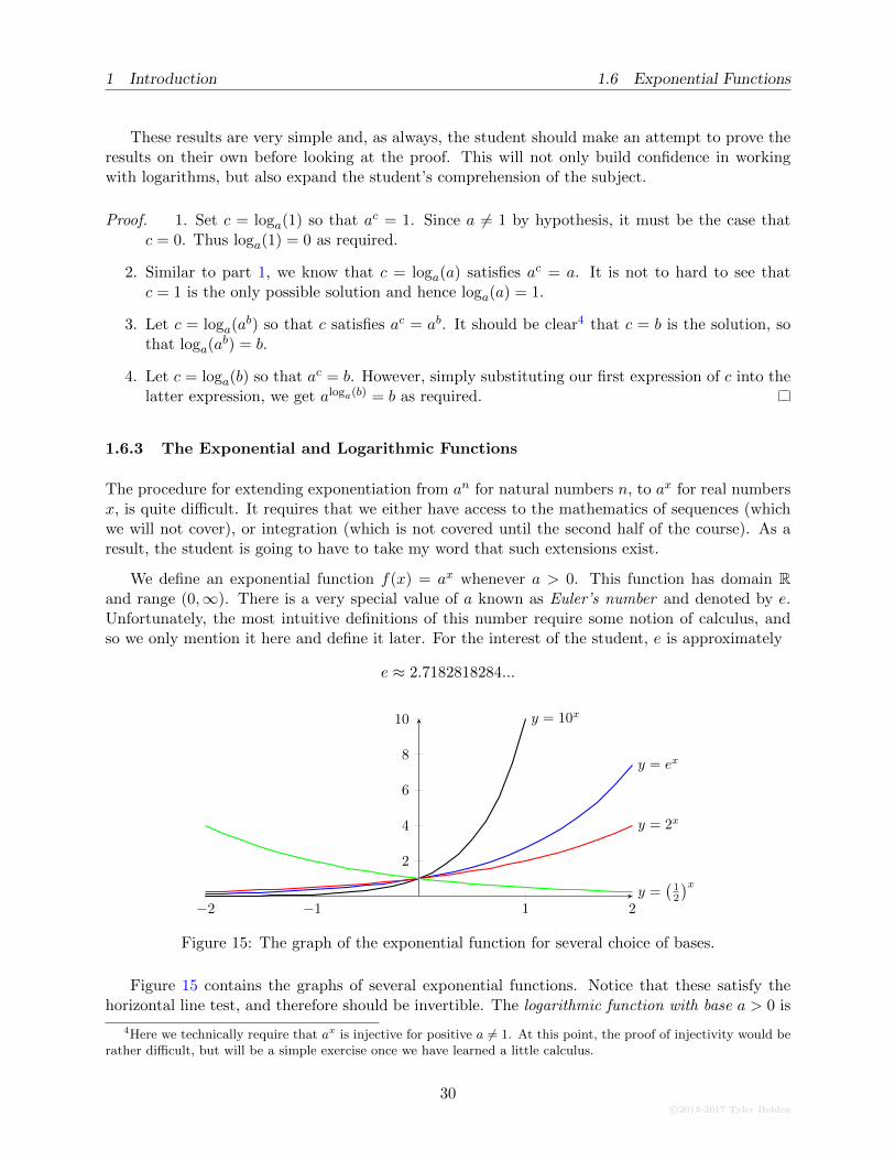
We define an exponential function f(x) = ax whenever a > 0. This function has domain Rand range (0,∞). There is a very special value of a known as Euler’s number and denoted by e.Unfortunately, the most intuitive definitions of this number require some notion of calculus, andso we only mention it here and define it later. For the interest of the student, e is approximately
e ≈ 2.7182818284...
−2 −1 1 2
2
4
6
8
10 y = 10x
y = ex
y = 2x
y =(12
)x
Figure 15: The graph of the exponential function for several choice of bases.
Figure 15 contains the graphs of several exponential functions. Notice that these satisfy thehorizontal line test, and therefore should be invertible. The logarithmic function with base a > 0 is
4Here we technically require that ax is injective for positive a 6= 1. At this point, the proof of injectivity would berather difficult, but will be a simple exercise once we have learned a little calculus.
30c©2013-2017 Tyler Holden
1.6 Exponential Functions 1 Introduction
the function g(x) = loga(x), which is designed to act as the inverse function for f(x) = ax. Indeed,using items 3 and 4 of Proposition 1.29 we see that
aloga(x) = x, loga(ax) = x
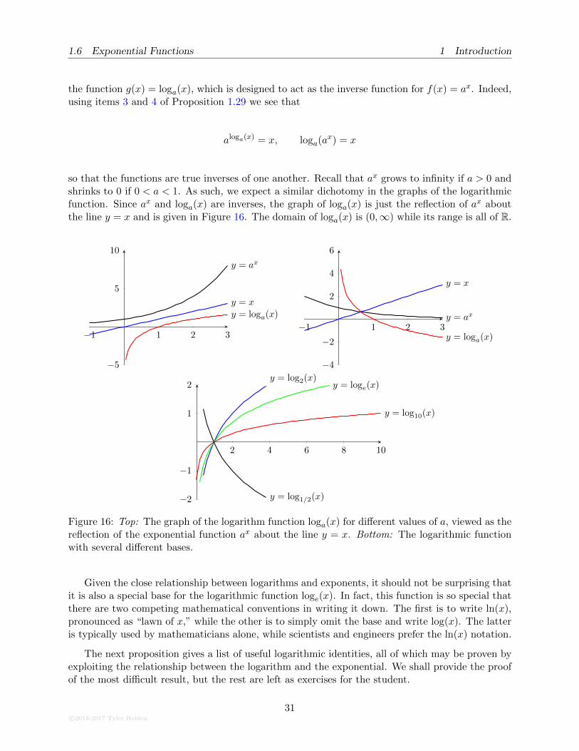
so that the functions are true inverses of one another. Recall that ax grows to infinity if a > 0 andshrinks to 0 if 0 < a < 1. As such, we expect a similar dichotomy in the graphs of the logarithmicfunction. Since ax and loga(x) are inverses, the graph of loga(x) is just the reflection of ax aboutthe line y = x and is given in Figure 16. The domain of loga(x) is (0,∞) while its range is all of R.
−1 1 2 3
−5
5
10
y = ax
y = x
y = loga(x)
−1 1 2 3
−4
−2
2
4
6
y = ax
y = x
y = loga(x)
2 4 6 8 10
−2
−1
1
2y = log2(x)
y = loge(x)
y = log10(x)
y = log1/2(x)
Figure 16: Top: The graph of the logarithm function loga(x) for different values of a, viewed as thereflection of the exponential function ax about the line y = x. Bottom: The logarithmic functionwith several different bases.
Given the close relationship between logarithms and exponents, it should not be surprising thatit is also a special base for the logarithmic function loge(x). In fact, this function is so special thatthere are two competing mathematical conventions in writing it down. The first is to write ln(x),pronounced as “lawn of x,” while the other is to simply omit the base and write log(x). The latteris typically used by mathematicians alone, while scientists and engineers prefer the ln(x) notation.
The next proposition gives a list of useful logarithmic identities, all of which may be proven byexploiting the relationship between the logarithm and the exponential. We shall provide the proofof the most difficult result, but the rest are left as exercises for the student.
c©2013-2017 Tyler Holden
31
2 Limits
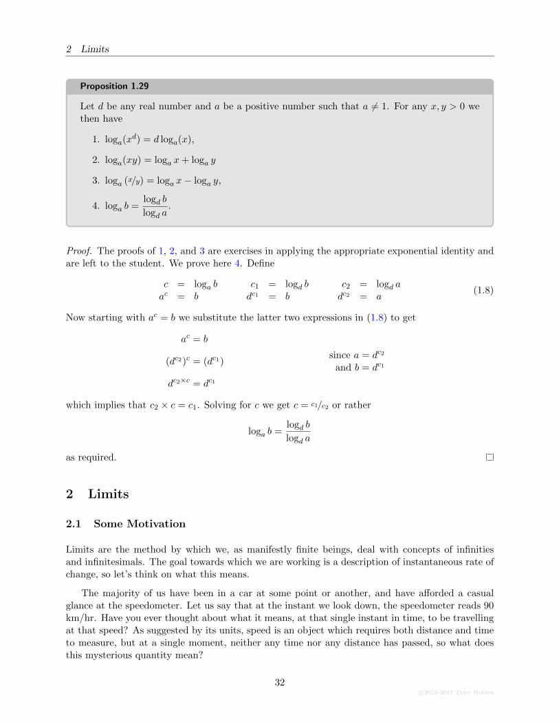
Proposition 1.29
Let d be any real number and a be a positive number such that a 6= 1. For any x, y > 0 wethen have
1. loga(xd) = d loga(x),
2. loga(xy) = loga x+ loga y
3. loga (x/y) = loga x− loga y,
4. loga b =logd b
logd a.
Proof. The proofs of 1, 2, and 3 are exercises in applying the appropriate exponential identity andare left to the student. We prove here 4. Define
c = loga b c1 = logd b c2 = logd aac = b dc1 = b dc2 = a
(1.8)
Now starting with ac = b we substitute the latter two expressions in (1.8) to get
ac = b
(dc2)c = (dc1)since a = dc2
and b = dc1
dc2×c = dc1
which implies that c2 × c = c1. Solving for c we get c = c1/c2 or rather
loga b =logd b
logd a
as required.
2 Limits
2.1 Some Motivation
Limits are the method by which we, as manifestly finite beings, deal with concepts of infinitiesand infinitesimals. The goal towards which we are working is a description of instantaneous rate ofchange, so let’s think on what this means.
The majority of us have been in a car at some point or another, and have afforded a casualglance at the speedometer. Let us say that at the instant we look down, the speedometer reads 90km/hr. Have you ever thought about what it means, at that single instant in time, to be travellingat that speed? As suggested by its units, speed is an object which requires both distance and timeto measure, but at a single moment, neither any time nor any distance has passed, so what doesthis mysterious quantity mean?
32c©2013-2017 Tyler Holden
2.1 Some Motivation 2 Limits
Despite my claims that the previous example should get you thinking about how the word“instantaneous” really affects a quantity, many of you will simply shrug aside my suggestions. Inanticipation of this reaction, what if we change the associated quantities around and instead ofthe instantaneous speed of a car, we discuss shopping! At any given point of time, somebody onthis planet is making a purchase. Assume that we were able to measure the rate at which peoplewere spending money, and I told you that at this moment in time the human species was globallyspending $140 million dollars an hour? What does this mean?
Now on the other hand, what if you were asked to determine the instantaneous speed of arace car at the instant its front bumper passes a finish line? Being clever students, you decide tomeasure how far the car has travelled in the minute before it hits the finish line, and get a resultof 1500 meters. Hence the car was travelling
1500 metres
1 minute× 1 kilometre
1000 metres× 60 minutes
1 hour=
90 kilometres
1 hour.
But what if the cars speed was not constant during that minute? What if the driver accelerated atthe end? You decide that you can get a better estimate of the speed at the finish line by insteadjust looking at how far the car travelled in the single second before the car hit the finish line. Thistime the car travelled 30 metres, so you calculate
30 metres
1 second=
108 kilometres
1 hour.
But still, this does not account for any change in acceleration which occurred in the last second.Your guess of 108 km/hr is probably close, but close is not good enough in mathematics! So youtry again by measuring the distance after 0.1 seconds, then 0.01 seconds, and so on , but no matterhow hard you try you cannot get the exact speed because there is always the chance that the carwas not travelling at a constant speed during your measurements. Nonetheless, we know there mustbe an answer: the car was travelling at some speed, so what is it? Limits provide the solution.
2.1.1 Intuition
Limits are the mathematical device which allow us to infer information about a point by analyzinginformation about well-behaved points nearby. Let f(x) be an arbitrary function and c ∈ R. Wesay that “the limit of f(x) as x approaches c is equal to L” if, whenever we let x get arbitrarilyclose to c then f(x) gets arbitrarily close to L. This is written as
limx→c
f(x) = L.
The best way to gain an intuitive understanding of limits is to see a few examples. We warn thestudent that this first example is rather nicely behaved and fails to capture why we use limits.Nonetheless, simple examples are often the best for getting a grasp as to how something works.
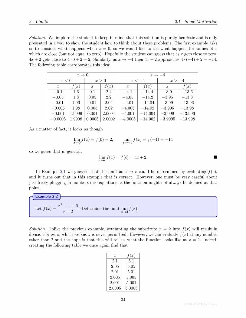
Example 2.1
Consider the function f(x) = 4x+ 2. Determine the limits
limx→0
f(x), limx→−4
f(x), limx→5
f(x).
Form a hypothesis as to what the limit is as x→ c for any value of c.
c©2013-2017 Tyler Holden
33
2 Limits 2.1 Some Motivation
Solution. We implore the student to keep in mind that this solution is purely heuristic and is onlypresented in a way to show the student how to think about these problems. The first example asksus to consider what happens when x = 0, so we would like to see what happens for values of xwhich are close (but not equal to zero). Hopefully the student can guess that as x gets close to zero,4x+ 2 gets close to 4 · 0 + 2 = 2. Similarly, as x→ −4 then 4x+ 2 approaches 4 · (−4) + 2 = −14.The following table corroborates this idea:
x→ 0 x→ −4
x < 0 x > 0 x < −4 x > −4
x f(x) x f(x) x f(x) x f(x)
−0.1 1.6 0.1 2.4 −4.1 −14.4 −3.9 −13.6−0.05 1.8 0.05 2.2 −4.05 −14.2 −3.95 −13.8−0.01 1.96 0.01 2.04 −4.01 −14.04 −3.99 −13.96−0.005 1.98 0.005 2.02 −4.005 −14.02 −3.995 −13.98−0.001 1.9996 0.001 2.0004 −4.001 −14.004 −3.999 −13.996−0.0005 1.9998 0.0005 2.0002 −4.0005 −14.002 −3.9995 −13.998
.
As a matter of fact, it looks as though
limx→0
f(x) = f(0) = 2, limx→−4
f(x) = f(−4) = −14
so we guess that in general,
limx→c
f(x) = f(c) = 4c+ 2. �
In Example 2.1 we guessed that the limit as x → c could be determined by evaluating f(c),and it turns out that in this example that is correct. However, one must be very careful aboutjust freely plugging in numbers into equations as the function might not always be defined at thatpoint.
Example 2.2
Let f(x) =x2 + x− 6
x− 2. Determine the limit lim
x→2f(x).
Solution. Unlike the previous example, attempting the substitute x = 2 into f(x) will result indivision-by-zero, which we know is never permitted. However, we can evaluate f(x) at any numberother than 2 and the hope is that this will tell us what the function looks like at x = 2. Indeed,creating the following table we once again find that
x f(x)
2.1 5.12.05 5.052.01 5.012.005 5.0052.001 5.0012.0005 5.0005
34c©2013-2017 Tyler Holden
2.1 Some Motivation 2 Limits
so it certainly appears as though f(x) is approaching 5. Indeed, if x 6= 2 then we may factor f(x)as
x2 + x− 6
x− 2=
(x+ 3)(x− 2)
x− 2= x+ 3
and the behaviour of this function as x→ 2 agrees with our observations. �
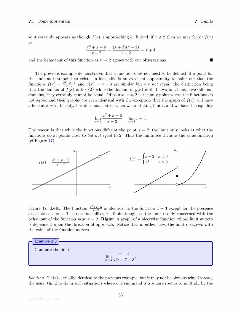
The previous example demonstrates that a function does not need to be defined at a point forthe limit at that point to exist. In fact, this is an excellent opportunity to point out that thefunctions f(x) = x2+x−6
x−2 and g(x) = x + 3 are similar but are not equal : the distinction beingthat the domain of f(x) is R \ {2} while the domain of g(x) is R. If two functions have differentdomains, they certainly cannot be equal! Of course, x = 2 is the only point where the functions donot agree, and their graphs are even identical with the exception that the graph of f(x) will havea hole at x = 2. Luckily, this does not matter when we are taking limits, and we have the equality
limx→2
x2 + x− 6
x− 2= lim
x→2x+ 3.
The reason is that while the functions differ at the point x = 2, the limit only looks at what thefunctions do at points close to but not equal to 2. Thus the limits see them as the same function(cf Figure 17).
x
y
f(x) =x2 + x− 6
x− 2
x
y
f(x) =
{x+ 2 x < 0
x2 x > 0
Figure 17: Left: The function x2+x−6x−2 is identical to the function x + 3 except for the presence
of a hole at x = 2. This does not affect the limit though, as the limit is only concerned with thebehaviour of the function near x = 2. Right: A graph of a piecewise function whose limit at zerois dependent upon the direction of approach. Notice that in either case, the limit disagrees withthe value of the function at zero.
Example 2.3
Compute the limit
limx→2
x− 2√x+ 7− 3
.
Solution. This is actually identical to the previous example, but it may not be obvious why. Instead,the usual thing to do in such situations where one summand is a square root is to multiply by the
c©2013-2017 Tyler Holden
35
2 Limits 2.2 One Sided Limits
conjugate. In this case,√x+ 7 + 3. In that case we have
limx→2
x− 2√x+ 7− 3
√x+ 7 + 3√x+ 7 + 3
= limx→2
(x− 2)(√x+ 7 + 3)
(x+ 7)− 9
= limx→2
x− 2
x− 2
[√x+ 7 + 3
]
= limx→2
[√x+ 7 + 3
]= 6.
The reason this is identical to Example 2.2 is that
x− 2 = (x+ 7)− 9 =[√x+ 7− 3
] [√x+ 7 + 3
]
and so the steps we just iterated may be replaced by a much simpler cancellation argument. �
2.2 One Sided Limits
Implicit in our previous discussion of limits is that when we take x → c, we must get the sameanswer whether we are approaching from the left of c or the right of c. It is possible that approachingfrom the left and right actually give different values of the limit, as can be seen in Figure 17. Thisnaturally leads us to the idea of one-sided limits, where we restrict our attention to values of thefunction on only one side of the limiting point.
More generally, we will say that “the limit of f(x) as x approaches c from the right is L” ifwhenever x > c gets arbitrarily close to c, f(x) gets arbitrarily close to L. This is written insymbols as
limx→c+
f(x) = L.
Similarly, we say that “the limit of f(x) as x approaches c from the left is L” if whenever x < cgets arbitrarily close to c, f(x) gets arbitrarily close to L, and in this case we write
limx→c−
f(x) = L.
If both of the one-sided limits exist and are equal to the same value L, then the limit x→ c existsand is also equal L. There are plenty of examples where the two-sided limit does not exist, as ourfollowing examples demonstrate.
Example 2.4
Consider the function
f(x) =
x+ 2 x < 0
1 x = 0
x2 x > 0
.
Compute the limit of f(x) as x→ 0− and as x→ 0+. Does the two-sided limit exist?
Solution. We first look at the limit as x → 0−. In this case, we know that x is always less than0, so f(x) effectively looks like the function x + 2. As x → 0− we see that x + 2 → 2 and so weconclude that
limx→0−
f(x) = 2.
36c©2013-2017 Tyler Holden
2.2 One Sided Limits 2 Limits
On the other hand, the limit x → 0+ guarantees that x is always positive. Here, f(x) looks likethe function x2 and as x approaches 0, x2 approaches 0 as well, so
limx→0+
f(x) = 0.
Each one-sided limit exists, but they are not equal. Hence the two-sided limit does not exist. Thegraph of f(x) is given in Figure 17. �
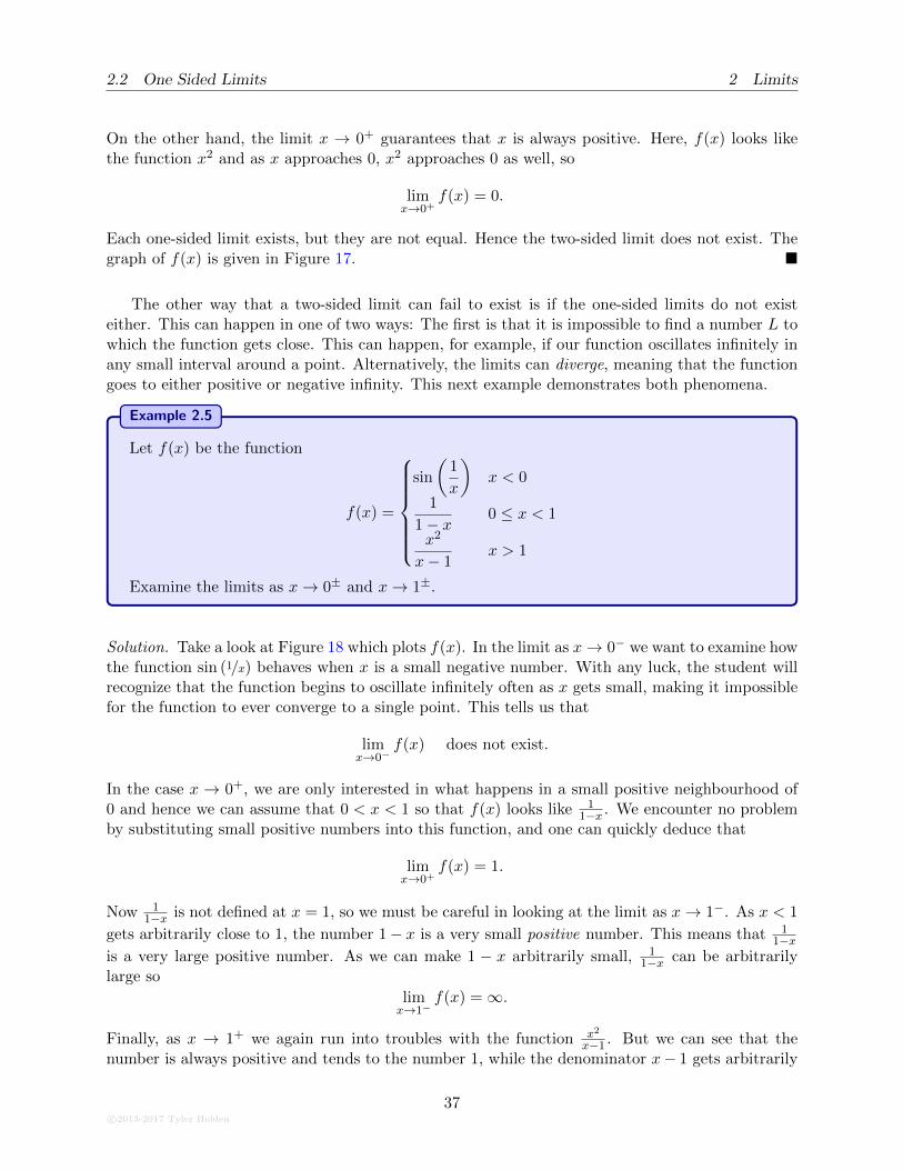
The other way that a two-sided limit can fail to exist is if the one-sided limits do not existeither. This can happen in one of two ways: The first is that it is impossible to find a number L towhich the function gets close. This can happen, for example, if our function oscillates infinitely inany small interval around a point. Alternatively, the limits can diverge, meaning that the functiongoes to either positive or negative infinity. This next example demonstrates both phenomena.
Example 2.5
Let f(x) be the function
f(x) =
sin
(1
x
)x < 0
1
1− x 0 ≤ x < 1
x2
x− 1x > 1
Examine the limits as x→ 0± and x→ 1±.
Solution. Take a look at Figure 18 which plots f(x). In the limit as x→ 0− we want to examine howthe function sin (1/x) behaves when x is a small negative number. With any luck, the student willrecognize that the function begins to oscillate infinitely often as x gets small, making it impossiblefor the function to ever converge to a single point. This tells us that
limx→0−
f(x) does not exist.
In the case x → 0+, we are only interested in what happens in a small positive neighbourhood of0 and hence we can assume that 0 < x < 1 so that f(x) looks like 1
1−x . We encounter no problemby substituting small positive numbers into this function, and one can quickly deduce that
limx→0+
f(x) = 1.
Now 11−x is not defined at x = 1, so we must be careful in looking at the limit as x→ 1−. As x < 1
gets arbitrarily close to 1, the number 1− x is a very small positive number. This means that 11−x
is a very large positive number. As we can make 1 − x arbitrarily small, 11−x can be arbitrarily
large so
limx→1−
f(x) =∞.
Finally, as x → 1+ we again run into troubles with the function x2
x−1 . But we can see that thenumber is always positive and tends to the number 1, while the denominator x− 1 gets arbitrarily
c©2013-2017 Tyler Holden
37
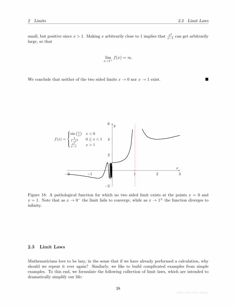
2 Limits 2.3 Limit Laws
small, but positive since x > 1. Making x arbitrarily close to 1 implies that x2
x−1 can get arbitrarilylarge, so that
limx→1+
f(x) =∞.
We conclude that neither of the two sided limits x→ 0 nor x→ 1 exist. �
−2 −1 1 2 3
−2
2
4
6
f(x) =
sin(1x
)x < 0
11−x2 0 ≤ x < 1x2
x−1 x > 1
x
y
Figure 18: A pathological function for which no two sided limit exists at the points x = 0 andx = 1. Note that as x → 0− the limit fails to converge, while as x → 1± the function diverges toinfinity.
2.3 Limit Laws
Mathematicians love to be lazy, in the sense that if we have already performed a calculation, whyshould we repeat it ever again? Similarly, we like to build complicated examples from simpleexamples. To this end, we formulate the following collection of limit laws, which are intended todramatically simplify our life:
38c©2013-2017 Tyler Holden
2.3 Limit Laws 2 Limits
Theorem 2.6: Limit Laws
If f(x) and g(x) be two functions, and c ∈ R such that
limx→c
f(x), limx→c
g(x)
both exist, then
1. limx→c
[αf(x)] = α limx→c
f(x),
2. limx→c
[f(x)± g(x)] =[limx→c
f(x)]±[limx→c
g(x)],
3. limx→c
[f(x)g(x)] =[limx→c
f(x)] [
limx→c
g(x)],
4. limx→c
[f(x)
g(x)
]=
limx→c f(x)
limx→c g(x)if limx→c
g(x) 6= 0
It is crucial that both limits must exist. It is a common mistake for students to gleefully attemptto apply the above limits laws in instances in which it is not permitted. For example, the followingIS NOT CORRECT:
limx→0
x2 sin
(1
x
)=[
limx→0
x2] [
limx→0
sin
(1
x
)]= 0×
[limx→0
sin
(1
x
)]= 0.
Interestingly, this is the correct answer, but for all the wrong reasons. Hence this solution isabsolutely incorrect.
Example 2.7
Compute the limit
limx→1
x4 + 7x+ 2
x− 4.
Solution. We would like to say that this is the limit of the quotient, and this will be the case solong as the limit of the numerator and denominator both exist, and the denominator is non-zero.For the numerator, we can again use the Limit Laws to break this into a sum of limits:
limx→1
[x4 + 7x+ 2
]= lim
x→1x4 + 7 lim
x→1x+ lim
x→12
=[
limx→1
x]4
+ 7[
limx→1
x]
+ 2[
limx→1
1]
= 1 + 7 + 2 = 10.
Similarly, the denominator gives
limx→1
[x− 4] = 1− 4 = −3.
Since both limits exist and the denominator is non-zero, we can apply the quotient Limit Law to
c©2013-2017 Tyler Holden
39
2 Limits 2.3 Limit Laws
get
limx→1
x4 + 7x+ 2
x− 4=
limx→1
x4 + 7x+ 2
limx→1
x− 4= −10
3. �
A similar argument to the previous example is the following theorem:
Theorem 2.8
If f(x) = p(x)q(x) is any rational functions (so that p(x) and q(x) are polynomials), and c ∈ R
is such that q(c) 6= 0 then
limx→c
p(x)
q(x)=p(c)
q(c).
Proof. The key is to first show this for polynomials and apply the limit laws. We shall assume apriori that
limx→c
x = c.
Now let p(x) = anxn + an−1x
n−1 + · · ·+ a1x+ a0 be an arbitrary polynomial. Certainly the limitof each aix
i exists, and so the limit laws imply that
limx→c
p(x) = limx→c
[anxn + · · ·+ a1x+ a0]
= an
[limx→c
x]n
+ an−1
[limx→c
x]n−1
+ · · ·+ a1
[limx→c
x]
+ a0
= ancn + an−1c
n−1 + · · ·+ a1c+ a0
= p(c).
Thus the result holds for any polynomial. Now if p(x) and q(x) are two polynomials and q(c) 6= 0,then the limit laws for quotients implies
limx→c
p(x)
q(x)=
limx→c
p(x)
limx→c
q(x)=p(c)
q(c).
Example 2.9
Determine the limit
limx→0
sin2(x)
1− cos(x).
Solution. On first glance, we are unable to substitute x = 0 into this equation since it would causeus to divide by zero. Instead, we recall that sin2(x) = (1 − cos2(x)) = (1 − cos(x))(1 + cos(x)) sothat
limx→0
sin2(x)
1− cos(x)= lim
x→0
(1− cos(x))(1 + cos(x))
1− cos(x)
= limx→0
[1 + cos(x)] = 2. �
40c©2013-2017 Tyler Holden
2.4 The Squeeze Theorem 2 Limits
Example 2.10
Determine the limit
limt→0
√1 + t−
√1− t
t.
Solution. When one finds that an expression involving square roots is proving difficult, it is oftena good idea to multiply by a conjugate form which places the square roots into a more amenableposition. In this instance, notice that
(√1 + t−
√1− t
) √1 + t+√
1− t√1 + t+
√1− t =
(1 + t)− (1− t)√1 + t−
√1− t =
2t√1 + t+
√1− t .
Hence our limit becomes
limt→0
√1 + t−
√1− t
t= lim
t→0
2t
t(√
1 + t+√
1− t)
= limt→0
2√1 + t+
√1− t
= 1. �
Example 2.11
Compute the limit
limh→0
(x+ h)2 − x2
h
Solution. Notice here that the variable of the limit is h rather than x! Since we cannot justsubstitute h = 0 into this equation, we must manipulate the expression to see if we can derive amore meaningful representative. Expanding the denominator we get
limh→0
(x+ h)2 − x2
h= lim
h→0
x2 + 2xh+ h2 − x2
h
= limh→0
2xh+ h2
h
= limh→0
2x+ h
= 2x. �
Expressions such as these will prove supremely useful when we cover derivatives.
2.4 The Squeeze Theorem
The Squeeze Theorem allows us to determine troublesome limits by bounded one function in termsof two other functions which converge to the same point.
c©2013-2017 Tyler Holden
41
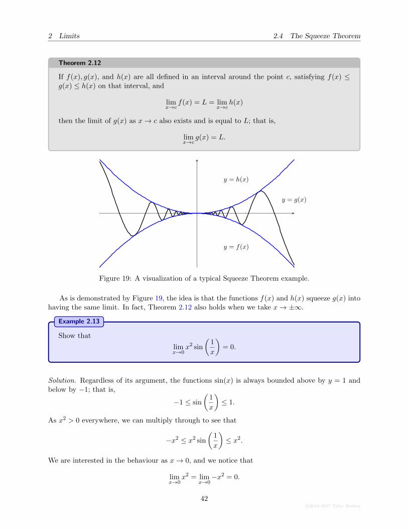
2 Limits 2.4 The Squeeze Theorem
Theorem 2.12
If f(x), g(x), and h(x) are all defined in an interval around the point c, satisfying f(x) ≤g(x) ≤ h(x) on that interval, and
limx→c
f(x) = L = limx→c
h(x)
then the limit of g(x) as x→ c also exists and is equal to L; that is,
limx→c
g(x) = L.
y = h(x)
y = f(x)
y = g(x)
Figure 19: A visualization of a typical Squeeze Theorem example.
As is demonstrated by Figure 19, the idea is that the functions f(x) and h(x) squeeze g(x) intohaving the same limit. In fact, Theorem 2.12 also holds when we take x→ ±∞.
Example 2.13
Show that
limx→0
x2 sin
(1
x
)= 0.
Solution. Regardless of its argument, the functions sin(x) is always bounded above by y = 1 andbelow by −1; that is,
−1 ≤ sin
(1
x
)≤ 1.
As x2 > 0 everywhere, we can multiply through to see that
−x2 ≤ x2 sin
(1
x
)≤ x2.
We are interested in the behaviour as x→ 0, and we notice that
limx→0
x2 = limx→0−x2 = 0.
42c©2013-2017 Tyler Holden
2.5 Infinite Limits 2 Limits
The Squeeze Theorem thus applies and we get
limx→0
x2 sin
(1
x
)= 0
as required. �
Example 2.14
Determine limx→∞
cos(x2)
x2 + 1.
Solution. We know that −1 ≤ cos(x2) ≤ 1 for all x, so
− 1
x2 + 1≤ cos(x2)
x2 + 1≤ 1
x2 + 1.
It is straightforward to check that
limx→∞
± 1
x2 + 1= 0,
so by the Squeeze Theorem we conclude that
limx→∞
cos(x2)
x2 + 1= 0. �
Exercise
1. If limx→0|f(x)| = 0 then lim
x→0f(x) = 0. [Hint: Convince yourself that −|f(x)| ≤ f(x) ≤
|f(x)|.]
2. If f(x) is bounded (so that there is some M > 0 with |f(x)| < M for all x) andlimx→0
g(x) = 0 then limx→0
f(x)g(x) = 0.
2.5 Infinite Limits
There are two ways in which to consider “limits at infinity:” either the function itself can divergeto infinity, or we can take a limit as x→ ±∞. The following sections will discuss this behaviour.
2.5.1 Vertical Asymptotes
There are functions which are singular at a point x = c, and these can sometimes result in ourlimits being infinite. For example, the function f(x) = 1/x becomes positively (resp. negatively)large when x > 0 (resp. x < 0) is small. So in this instance we have
limx→0+
1
x=∞, lim
x→0−
1
x= −∞. (2.1)
c©2013-2017 Tyler Holden
43
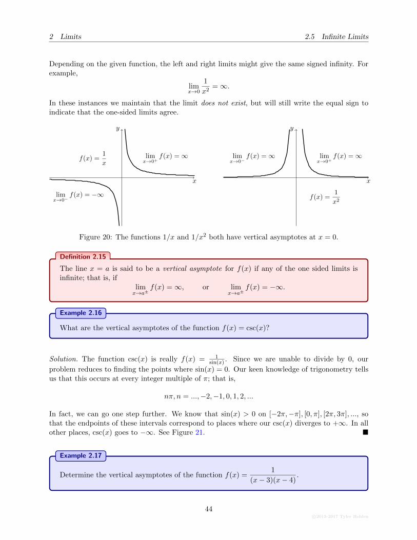
2 Limits 2.5 Infinite Limits
Depending on the given function, the left and right limits might give the same signed infinity. Forexample,
limx→0
1
x2=∞.
In these instances we maintain that the limit does not exist, but will still write the equal sign toindicate that the one-sided limits agree.
x
y
f(x) =1
xlim
x→0+f(x) =∞
limx→0−
f(x) = −∞
x
y
f(x) =1
x2
limx→0+
f(x) =∞limx→0−
f(x) =∞
Figure 20: The functions 1/x and 1/x2 both have vertical asymptotes at x = 0.
Definition 2.15
The line x = a is said to be a vertical asymptote for f(x) if any of the one sided limits isinfinite; that is, if
limx→a±
f(x) =∞, or limx→a±
f(x) = −∞.
Example 2.16
What are the vertical asymptotes of the function f(x) = csc(x)?
Solution. The function csc(x) is really f(x) = 1sin(x) . Since we are unable to divide by 0, our
problem reduces to finding the points where sin(x) = 0. Our keen knowledge of trigonometry tellsus that this occurs at every integer multiple of π; that is,
nπ, n = ...,−2,−1, 0, 1, 2, ...
In fact, we can go one step further. We know that sin(x) > 0 on [−2π,−π], [0, π], [2π, 3π], ..., sothat the endpoints of these intervals correspond to places where our csc(x) diverges to +∞. In allother places, csc(x) goes to −∞. See Figure 21. �
Example 2.17
Determine the vertical asymptotes of the function f(x) =1
(x− 3)(x− 4).
44c©2013-2017 Tyler Holden
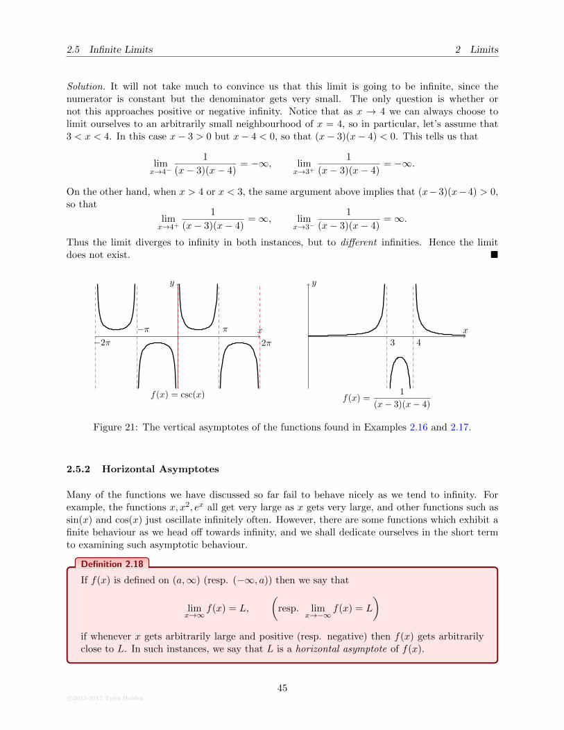
2.5 Infinite Limits 2 Limits
Solution. It will not take much to convince us that this limit is going to be infinite, since thenumerator is constant but the denominator gets very small. The only question is whether ornot this approaches positive or negative infinity. Notice that as x → 4 we can always choose tolimit ourselves to an arbitrarily small neighbourhood of x = 4, so in particular, let’s assume that3 < x < 4. In this case x− 3 > 0 but x− 4 < 0, so that (x− 3)(x− 4) < 0. This tells us that
limx→4−
1
(x− 3)(x− 4)= −∞, lim
x→3+
1
(x− 3)(x− 4)= −∞.
On the other hand, when x > 4 or x < 3, the same argument above implies that (x−3)(x−4) > 0,so that
limx→4+
1
(x− 3)(x− 4)=∞, lim
x→3−
1
(x− 3)(x− 4)=∞.
Thus the limit diverges to infinity in both instances, but to different infinities. Hence the limitdoes not exist. �
x
y
−2π 2π
−π π
f(x) = csc(x)
x
y
3 4
f(x) =1
(x− 3)(x− 4)
Figure 21: The vertical asymptotes of the functions found in Examples 2.16 and 2.17.
2.5.2 Horizontal Asymptotes
Many of the functions we have discussed so far fail to behave nicely as we tend to infinity. Forexample, the functions x, x2, ex all get very large as x gets very large, and other functions such assin(x) and cos(x) just oscillate infinitely often. However, there are some functions which exhibit afinite behaviour as we head off towards infinity, and we shall dedicate ourselves in the short termto examining such asymptotic behaviour.
Definition 2.18
If f(x) is defined on (a,∞) (resp. (−∞, a)) then we say that
limx→∞
f(x) = L,
(resp. lim
x→−∞f(x) = L
)
if whenever x gets arbitrarily large and positive (resp. negative) then f(x) gets arbitrarilyclose to L. In such instances, we say that L is a horizontal asymptote of f(x).
c©2013-2017 Tyler Holden
45
2 Limits 2.5 Infinite Limits
To re-iterate, polynomial and trigonometric functions are not going to have finite limits atinfinity, since the polynomial functions diverge and the polynomials oscillate without bound. Sowhat are examples of functions which do have finite? Well to start, for any p > 0, we have that
limx→±∞
1
xp= 0.
This gives us a large number of unexciting functions with finite asymptotics. However, thisresult is of far more interest when used on other functions.
Example 2.19
Determine the limit limx→∞
3x2 + 6x− 1
4x2 − 2.
Solution. It is rather unwieldy to deal with this function as written, since both the numerator anddenominator become arbitrarily large and it is difficult to see what “cancellations” might occur.Instead, let us multiply and divide by the quantity 1
x2to get
limx→∞
3x2 + 6x− 1
4x2 − 2
1/x2
1/x2= lim
x→∞
3x2/x2 + 6x/x2 − 1/x2
4x2/x2 − 2/x2
= limx→∞
3 + 6/x− 1/x2
4− 2/x2
=3 + lim
x→∞
6
x− limx→∞
1
x2
4− limx→∞
2
x2
=3
4
where in the last line we have used the fact that the quantities 1x and 1
x2go to zero as x→∞. �
This suggests a general strategy for determining the limits of rational functions:
Strategy for Rational Functions
1. Determine the highest power n which occurs in the functions,
2. Multiply and divide by 1/xn,
3. Take the limit as x→∞ using the fact that 1/xp → 0 for all p > 0.
In the case of rational functions, this actually gives an incredibly convenient way of looking ata function and determining its asymptotic limit:
46c©2013-2017 Tyler Holden
2.5 Infinite Limits 2 Limits
Theorem 2.20
Consider the rational function f(x) =anx
n + · · ·+ a1x+ a0
bmxm + · · ·+ b1x+ b0.
1. If n > m then limx→∞
f(x) =∞.
2. If n < m then limx→∞
f(x) = 0
3. If n = m then limx→∞
f(x) =anbm
.
As a matter of fact, the general strategy for determining the asymptotics of a function amountsto ascertaining which component of the function grows fastest. If the numerator grows fastest thefunction diverges, if the denominator grows fastest the function converges to 0, and if the numeratorand denominator grow at the same rate, the function can attain a non-zero limit.
Example 2.21
Find the limit
limx→∞
ex + e−x
ex − e−x .
Solution. Our goal is to divide by the “highest order term.” In this case, that corresponds to theex term. Can you see why this is true? In essence, we would like to get rid of the things the explodeas x→∞, and keep the things that get small. This means we want to get rid of ex and keep e−x
which is why we divide by ex. We thus get
limx→∞
ex + e−x
ex − e−xe−x
e−x= lim
x→∞
1 + e−2x
1− e−2x
=1
1= 1. �
Exercise
What are the limits
limx→0±
ex + e−x
ex − e−x , limx→−∞
ex + e−x
ex − e−x .
Example 2.22
Determine the horizontal asymptotes of the function f(x) =
√4x2 + 5
x+ 2.
Solution. The square root here presents many difficulties. In particular, while the numerator willalways be positive, the denominator will change sign. We must ensure that we account for this.Furthermore, while the numerator might have an x2 component, the square root means that thenumerator effectively acts as
√x2 = |x| so only grows linearly rather than quadratically.
c©2013-2017 Tyler Holden
47
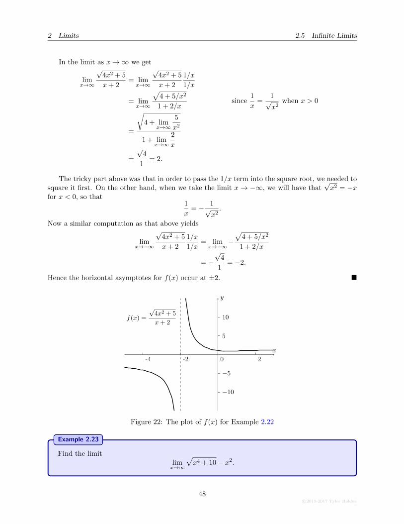
2 Limits 2.5 Infinite Limits
In the limit as x→∞ we get
limx→∞
√4x2 + 5
x+ 2= lim
x→∞
√4x2 + 5
x+ 2
1/x
1/x
= limx→∞
√4 + 5/x2
1 + 2/xsince
1
x=
1√x2
when x > 0
=
√4 + lim
x→∞
5
x2
1 + limx→∞
2
x
=
√4
1= 2.
The tricky part above was that in order to pass the 1/x term into the square root, we needed tosquare it first. On the other hand, when we take the limit x→ −∞, we will have that
√x2 = −x
for x < 0, so that1
x= − 1√
x2.
Now a similar computation as that above yields
limx→−∞
√4x2 + 5
x+ 2
1/x
1/x= lim
x→−∞−√
4 + 5/x2
1 + 2/x
= −√
4
1= −2.
Hence the horizontal asymptotes for f(x) occur at ±2. �
x
y
-4 -2 0 2
−10
−5
5
10f(x) =
√4x2 + 5
x+ 2
Figure 22: The plot of f(x) for Example 2.22
Example 2.23
Find the limitlimx→∞
√x4 + 10− x2.
48c©2013-2017 Tyler Holden
2.6 Continuity 2 Limits
Solution. At first glance, this may look like it diverges, but be careful! The fact that there is an x4
term under a square root means√x4 + 10 behaves as x2 as x gets very big. This term will, in the
long term, cancel the effect of the x2 leaving a finite answer. In order to make this more precise,we multiply by the conjugate
limx→∞
[(√x4 + 10− x2
)(√x4 + 10 + x2
√x4 + 10 + x2
)]= lim
x→∞
x4 + 10− x4
√x4 + 10 + x2
= limx→∞
10√x4 + 10 + x2
Now the bottom term goes goes to ∞ as x→∞, so the whole limit goes to zero, and we conclude
limx→∞
√x4 + 10− x2 = 0. �
2.6 Continuity
Of the examples seen thus far, we have seen instances in which the limit was easily computableby simply substituting the limiting value into the function, and other more pathological exampleswherein this was not possible. The former examples are particularly special, not only becauseof the simplicity of evaluating limits, but because they tell us that the function is, in a sense,“well-behaved” at that limiting point.
Definition 2.24
We say that a function f(x) is continuous at the point c ∈ R if
limx→c
f(x) = f(c).
If the function f(x) is continuous at all points in R, we say that it is continuous.
In Example 2.7 we showed that
limx→1
x4 + 7x+ 2
x− 4= −10/3.
Substituting x = 1 into this limiting function, we get
(1)4 + 7(1) + 2
(1)− 4=
10
−3.
so that the function f(x) = (x4 + 7x+ 2)/(x− 4) is continuous at the point x = 1.
In fact, we have already seen entire families of continuous functions. Recall from Theorem 2.8that if p(x) and q(x) are polynomials and q(c) 6= 0 then
limx→c
p(x)
q(x)=p(c)
q(c).
This implies that all rational functions are continuous at points where their denominator does notvanish.
c©2013-2017 Tyler Holden
49
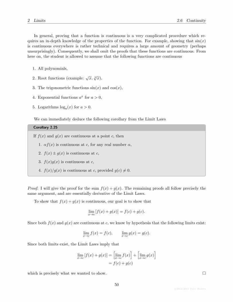
2 Limits 2.6 Continuity
In general, proving that a function is continuous is a very complicated procedure which re-quires an in-depth knowledge of the properties of the function. For example, showing that sin(x)is continuous everywhere is rather technical and requires a large amount of geometry (perhapsunsurprisingly). Consequently, we shall omit the proofs that these functions are continuous. Fromhere on, the student is allowed to assume that the following functions are continuous
1. All polynomials,
2. Root functions (example:√x, 3√x),
3. The trigonometric functions sin(x) and cos(x),
4. Exponential functions ax for a > 0,
5. Logarithms loga(x) for a > 0.
We can immediately deduce the following corollary from the Limit Laws
Corollary 2.25
If f(x) and g(x) are continuous at a point c, then
1. αf(x) is continuous at c, for any real number α,
2. f(x)± g(x) is continuous at c,
3. f(x)g(x) is continuous at c,
4. f(x)/g(x) is continuous at c, provided g(c) 6= 0.
Proof. I will give the proof for the sum f(x) + g(x). The remaining proofs all follow precisely thesame argument, and are essentially derivative of the Limit Laws.
To show that f(x) + g(x) is continuous, our goal is to show that
limx→c
[f(x) + g(x)] = f(c) + g(c).
Since both f(x) and g(x) are continuous at c, we know by hypothesis that the following limits exist:
limx→c
f(x) = f(c), limx→c
g(x) = g(c).
Since both limits exist, the Limit Laws imply that
limx→c
[f(x) + g(x)] =[limx→c
f(x)]
+[limx→c
g(x)]
= f(c) + g(c)
which is precisely what we wanted to show.
50c©2013-2017 Tyler Holden
2.6 Continuity 2 Limits
Example 2.26
Consider the function f(x) =x2 + 6x+ 2
(x+ 4)(x2 − 1). Determine the points where f(x) is not
continuous.
Solution. This function fails to be continuous wherever its denominator vanishes. We may factor(x + 4)(x2 − 1) = (x + 4)(x − 1)(x + 1), which tells us that the points of discontinuity occur atx = −4,−1,+1. �
Combining Corollary 2.25 with the list of functions assumed to be continuous, we can immedi-ately generate very large families of continuous functions.
Example 2.27
Determine the limit limx→4
x2 +√x
2x cos(x).
Solution. The numerator x2 +√x is the sum of the continuous functions x2 and
√x, and hence
is itself continuous. Similarly, the denominator 2x cos(x) is a product of continuous functions andhence is continuous. The quotient will be continuous so long as the denominator does not vanishat x = 4, and indeed
limx→4
2x cos(x) = 24 cos(4) = 16 cos(4) 6= 0.
Thus the whole function (x2+√x)/(2x cos(x)) is continuous at x = 4 and the limit can be evaluated
by substitution:
limx→4
x2 +√x
2x cos(x)=
42 +√
4
24 cos(4)=
18
16 cos(4)=
9
8 cos(4). �
Composition of Functions: Arguably, our most powerful operation on functions is that ofcomposition, and it turns out that this will give us an incredible insight into what it means to becontinuous. Recall that f(x) is continuous at c if the limit can be evaluated by simple substitution.This may be alternatively written as
limx→c
f(x) = f(c) = f(
limx→c
x).
In a sense, it appears as though we are able to pass the limit inside of the function. In many ways,this is the true definition of continuity, so let’s see how this might be useful to solving problems.
Theorem 2.28
If g(x) has a limit as c, say limx→c
g(x) = L (note that g(x) does not need to be continuous),
and f(x) is continuous at L, then
limx→c
f(g(x)) = f(
limx→c
g(x)).
c©2013-2017 Tyler Holden
51
2 Limits 2.6 Continuity
When g(x) = x this reduces to the definition of continuity.
Example 2.29
Define the function
g(x) =
{x x 6= 0
2 x = 0.
Compute the limit limx→0
eg(x).
Solution. One might be tempted into thinking that eg(x) is continuous, but the fact that g(x) failsto be continuous means that this is not the case. Indeed, if we attempted to substitution we wouldfind that the limit would be eg(0) = e2 and this is not true (try graphing this and see for yourself).Instead, let us define f(x) = ex so that eg(x) = f(g(x)). We know that f(x) is then continuous, soby the previous theorem we have
limx→c
f(g(x)) = f(
limx→c
g(x))
= elimx→c
g(x)= e0 = 1. �
An immediate result of Theorem 2.28 is the following:
Corollary 2.30
If g(x) is continuous at c and f(x) is continuous at g(c) then f(g(x)) is continuous at c.
Proof. Because both f(x) and g(x) are continuous at the necessary points, we just keep passingthe limit into the arguments to see that
limx→c
f(g(x)) = f(
limx→c
g(x))
= f(g(
limx→c
x))
= f(g(c)).
Thus the composition of continuous functions is continuous. This can make complicated limitssimple to solve.
Example 2.31
Compute the limit limx→0
esin(x).
Solution. Setting f(x) = ex and g(x) = sin(x) we get that esin(x) = f(g(x)). Since both f(x) andg(x) are continuous, so too is f(g(x)) and the limit may be computed by simple substitution. Thuswe get
limx→0
esin(x) = esin(0) = e0 = 1. �
52c©2013-2017 Tyler Holden
2.6 Continuity 2 Limits
2.6.1 One-Sided Continuity and Failures of Continuity
Just as there are one sided limits, we can consequently have one-sided continuity.
Definition 2.32
We say that f(x) is continuous at c from the right (resp. from the left) if
limx→c+
f(x) = f(c),
(resp. lim
x→c−f(x) = f(c)
).
Certainly, any function which is continuous at c will be continuous from both the left and theright at c. For an example of a function which is only continuous from a single side, consider thefunction
f(x) =
{4x+ 2 x ≤ 0
−x x > 0.
At x = 0, f(x) has the value f(0) = 2, and has one sided limits
limx→0−
f(x) = 2, limx→0+
f(x) = 0.
This implies that f(x) is continuous from the left, as limx→0−
f(x) = f(0), but not from the right.
Example 2.33
Consider the function
f(x) =
{x|x| if x 6= 0
c if x = 0..
Determine the value of c such that f is continuous from the left at 0. What value of c makesf continuous from the right at 0?
Solution. All we need to do is determine the limit as x→ 0− and set c to be this number. In thislimit we may assume that x < 0, so that |x| = −x, and we get
limx→0−
f(x) = limx→0−
x
−x = limx→0−
−1 = −1.
so we set c = −1. Doing the same analysis for the limit as x→ 0+ we get c = 1. �
If a limit fails to exist then it certainly has no chance of being continuous. On the other hand,the function f(x) = (x − 3)/(x2 − x + 12) has a finite, two-sided limit at x = 3, but fails to becontinuous there since f(x) is not defined at x = 3. The fact that continuities seem inherently“worse” than other leads to a classification of discontinuities.
c©2013-2017 Tyler Holden
53
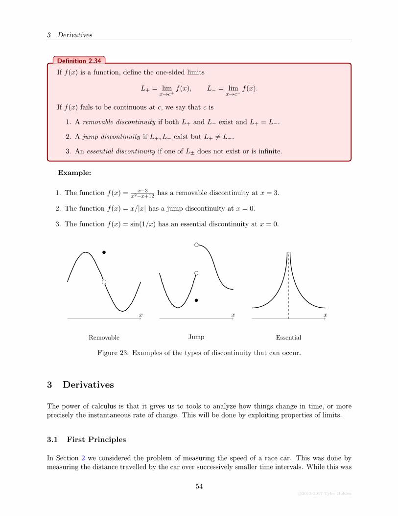
3 Derivatives
Definition 2.34
If f(x) is a function, define the one-sided limits
L+ = limx→c+
f(x), L− = limx→c−
f(x).
If f(x) fails to be continuous at c, we say that c is
1. A removable discontinuity if both L+ and L− exist and L+ = L−.
2. A jump discontinuity if L+, L− exist but L+ 6= L−.
3. An essential discontinuity if one of L± does not exist or is infinite.
Example:
1. The function f(x) = x−3x2−x+12
has a removable discontinuity at x = 3.
2. The function f(x) = x/|x| has a jump discontinuity at x = 0.
3. The function f(x) = sin(1/x) has an essential discontinuity at x = 0.
x
Removable
x
Jump
x
Essential
Figure 23: Examples of the types of discontinuity that can occur.
3 Derivatives
The power of calculus is that it gives us to tools to analyze how things change in time, or moreprecisely the instantaneous rate of change. This will be done by exploiting properties of limits.
3.1 First Principles
In Section 2 we considered the problem of measuring the speed of a race car. This was done bymeasuring the distance travelled by the car over successively smaller time intervals. While this was
54c©2013-2017 Tyler Holden
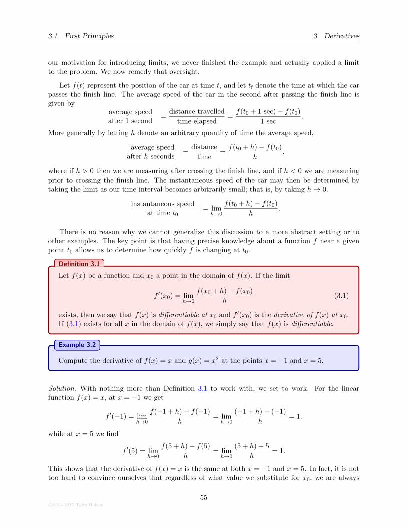
3.1 First Principles 3 Derivatives
our motivation for introducing limits, we never finished the example and actually applied a limitto the problem. We now remedy that oversight.
Let f(t) represent the position of the car at time t, and let tf denote the time at which the carpasses the finish line. The average speed of the car in the second after passing the finish line isgiven by
average speedafter 1 second
=distance travelled
time elapsed=f(t0 + 1 sec)− f(t0)
1 sec.
More generally by letting h denote an arbitrary quantity of time the average speed,
average speedafter h seconds
=distance
time=f(t0 + h)− f(t0)
h,
where if h > 0 then we are measuring after crossing the finish line, and if h < 0 we are measuringprior to crossing the finish line. The instantaneous speed of the car may then be determined bytaking the limit as our time interval becomes arbitrarily small; that is, by taking h→ 0.
instantaneous speedat time t0
= limh→0
f(t0 + h)− f(t0)
h.
There is no reason why we cannot generalize this discussion to a more abstract setting or toother examples. The key point is that having precise knowledge about a function f near a givenpoint t0 allows us to determine how quickly f is changing at t0.
Definition 3.1
Let f(x) be a function and x0 a point in the domain of f(x). If the limit
f ′(x0) = limh→0
f(x0 + h)− f(x0)
h(3.1)
exists, then we say that f(x) is differentiable at x0 and f ′(x0) is the derivative of f(x) at x0.If (3.1) exists for all x in the domain of f(x), we simply say that f(x) is differentiable.
Example 3.2
Compute the derivative of f(x) = x and g(x) = x2 at the points x = −1 and x = 5.
Solution. With nothing more than Definition 3.1 to work with, we set to work. For the linearfunction f(x) = x, at x = −1 we get
f ′(−1) = limh→0
f(−1 + h)− f(−1)
h= lim
h→0
(−1 + h)− (−1)
h= 1.
while at x = 5 we find
f ′(5) = limh→0
f(5 + h)− f(5)
h= lim
h→0
(5 + h)− 5
h= 1.
This shows that the derivative of f(x) = x is the same at both x = −1 and x = 5. In fact, it is nottoo hard to convince ourselves that regardless of what value we substitute for x0, we are always
c©2013-2017 Tyler Holden
55
3 Derivatives 3.1 First Principles
going to get f ′(x0) = 1. This is tantamount to the fact that f ′(x0) describes the rate of change ofthe function, and f(x) = x is function which is growing at a constant rate.
Before proceeding to the next example, let us try to anticipate the kind of solution we will seefrom the function g(x) = x2. The shape of the parabola seems to suggest that x2 is decreasingat x = −1 and so g′(−1) should be negative. On the other hand, g(x) is growing larger at x = 5implying that g′(5) should be positive. The necessary computations are slightly more complicated,but nothing beyond our capabilities:
g′(−1) = limh→0
g(−1 + h)− g(−1)
h= lim
h→0
(−1 + h)2 − (−1)2
h
= limh→0
(1− 2h+ h2)− 1
h= lim
h→0−2 + h
= −2
g′(5) = limh→0
g(5 + h)− g(5)
h= lim
h→0
(5 + h)2 − 52
h
= limh→0
h2 + 10h+ 25− 25
h= lim
h→0h+ 10
= 10.
The is precisely the behaviour we anticipated. Even further, the rate at which g(x) is growing atx = 5 is much faster than the speed at which it is decreasing at x = −1. This is corroborated bythe graph of g(x) = x2: we expect the magnitude of the rate of change of g(x) to increasing withthe magnitude of x. �
Example 3.3
Compute the derivative of the function f(x) =3x+ 2
x− 4at the point x = 5.
Solution. The behaviour of this function is not as transparent as that given in Example 3.2, so wemust trust in our calculations. As before, we apply Definition 3.1 to f(x) to find
f ′(5) = limh→0
f(5 + h)− f(5)
h= lim
h→0
3(5+h)+2(5+h)−4 − 17
h
= limh→0
3h+17h+1 − 17
h= lim
h→0
(3h+17)−(17h+17)h+1
hcommon denominator
= limh→0
−14h
h(h+ 1)= lim
h→0
−14
h+ 1
= −14.
This tells us that the function is decreasing at x = 5. �
56c©2013-2017 Tyler Holden

3.1 First Principles 3 Derivatives
The computations of the derivatives in Example 3.2 where redundant, requiring only smallchanges between the x = −1 and x = 5 cases. If instead of using a particular number, we let x = adescribe a general point, we could compute
f ′(a) = limx→a
f(x)− f(a)
x− a
= limx→a
x2 − a2
x− a= lim
x→a
(x+ a)(x− a)
x− a = limx→a
(x+ a)
= 2a.
This agrees with what we found when a = −1 and a = 5, but gives us the derivative at any pointa. Hence one can view the derivative of a function as a function itself, with
f ′(x) = limh→0
f(x+ h)− f(x)
h= lim
y→x
f(y)− f(x)
y − x .
In fact, this is where the word derivative comes from: the value of the function f ′(x) is derivedfrom that of f(x).
Exercise: How is the domain of f ′(x) related to f(x)? Must they always be the same? Orcan one be larger than the other?
3.1.1 The Geometry of the Derivative
We can visualize the derivative geometrically by examining the graph of f(x).
Definition 3.4
Consider the graph of a function f(x) and let a < b be distinct real numbers. The secantline from a to b is the unique straight line which passes through the points (a, f(a)) and(b, f(b)).
Of interest is the slope of this secant line, given by
mab =f(b)− f(a)
b− a .
In fact, this slope describes the average change in the value of f(x) between f(a) and f(b). We canget successively better approximations to the instantaneous rate of change of a function by takingthe distance between a and b to be successively smaller, and the instantaneous rate of change willbe given by taking a limit as a→ b. See Figure 24. Notice that in this limit the secant line becomesa tangent line; that is,
If f(x) is differentiable, the slope of the tangent line to the graph of f(x) at a is f ′(a).
c©2013-2017 Tyler Holden
57
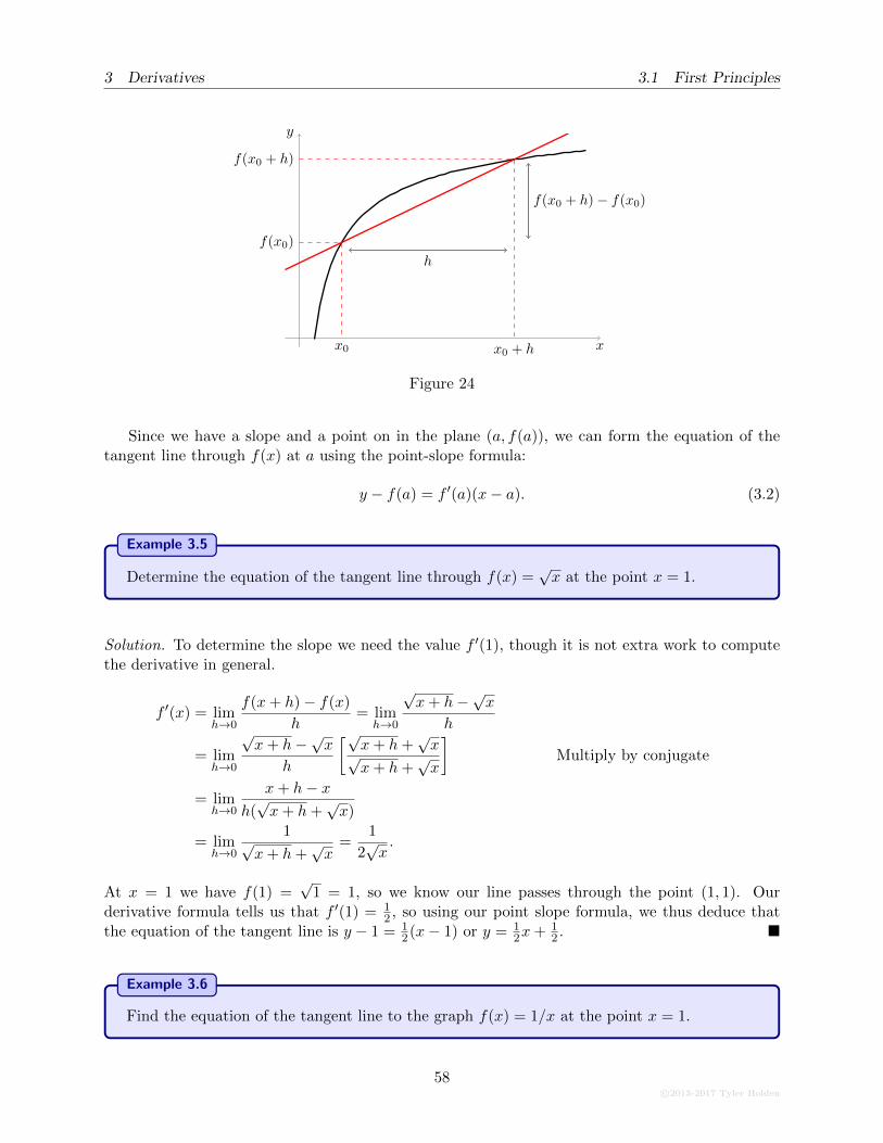
3 Derivatives 3.1 First Principles
x
y
f(x0)
x0
f(x0 + h)
x0 + h
h
f(x0 + h)− f(x0)
Figure 24
Since we have a slope and a point on in the plane (a, f(a)), we can form the equation of thetangent line through f(x) at a using the point-slope formula:
y − f(a) = f ′(a)(x− a). (3.2)
Example 3.5
Determine the equation of the tangent line through f(x) =√x at the point x = 1.
Solution. To determine the slope we need the value f ′(1), though it is not extra work to computethe derivative in general.
f ′(x) = limh→0
f(x+ h)− f(x)
h= lim
h→0
√x+ h−√x
h
= limh→0
√x+ h−√x
h
[√x+ h+
√x√
x+ h+√x
]Multiply by conjugate
= limh→0
x+ h− xh(√x+ h+
√x)
= limh→0
1√x+ h+
√x
=1
2√x.
At x = 1 we have f(1) =√
1 = 1, so we know our line passes through the point (1, 1). Ourderivative formula tells us that f ′(1) = 1
2 , so using our point slope formula, we thus deduce thatthe equation of the tangent line is y − 1 = 1
2(x− 1) or y = 12x+ 1
2 . �
Example 3.6
Find the equation of the tangent line to the graph f(x) = 1/x at the point x = 1.
58c©2013-2017 Tyler Holden
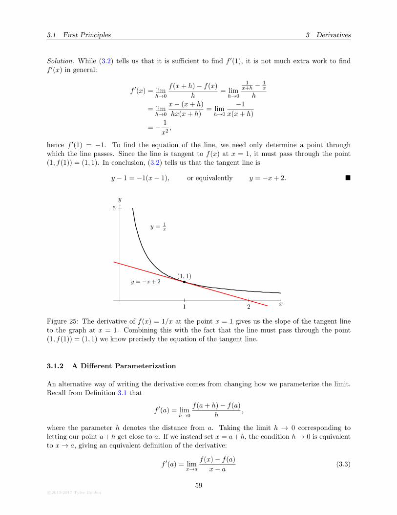
3.1 First Principles 3 Derivatives
Solution. While (3.2) tells us that it is sufficient to find f ′(1), it is not much extra work to findf ′(x) in general:
f ′(x) = limh→0
f(x+ h)− f(x)
h= lim
h→0
1x+h − 1
x
h
= limh→0
x− (x+ h)
hx(x+ h)= lim
h→0
−1
x(x+ h)
= − 1
x2,
hence f ′(1) = −1. To find the equation of the line, we need only determine a point throughwhich the line passes. Since the line is tangent to f(x) at x = 1, it must pass through the point(1, f(1)) = (1, 1). In conclusion, (3.2) tells us that the tangent line is
y − 1 = −1(x− 1), or equivalently y = −x+ 2. �
x
y
5
1 2
(1, 1)y = −x+ 2
y = 1x
Figure 25: The derivative of f(x) = 1/x at the point x = 1 gives us the slope of the tangent lineto the graph at x = 1. Combining this with the fact that the line must pass through the point(1, f(1)) = (1, 1) we know precisely the equation of the tangent line.
3.1.2 A Different Parameterization
An alternative way of writing the derivative comes from changing how we parameterize the limit.Recall from Definition 3.1 that
f ′(a) = limh→0
f(a+ h)− f(a)
h,
where the parameter h denotes the distance from a. Taking the limit h → 0 corresponding toletting our point a+h get close to a. If we instead set x = a+h, the condition h→ 0 is equivalentto x→ a, giving an equivalent definition of the derivative:
f ′(a) = limx→a
f(x)− f(a)
x− a (3.3)
c©2013-2017 Tyler Holden
59
3 Derivatives 3.1 First Principles
Example 3.7
Compute the derivative of the function f(x) = 9/x for any point a 6= 0 using (3.3).
Solution. Applying Equation (3.3) we get
f ′(a) = limx→a
f(x)− f(a)
x− a = limx→a
9/x− 9/a
x− a= lim
x→a
9(a− x)/xa
x− a = limx→a
−9
ax
= − 9
a2. �
3.1.3 Relating Variables and Leibniz Notation
Functions can be used to describe how one variable depends upon another. For example, theidentity y = x2 tells us precisely how the variable y depends upon the function x. Given a generalfunction f(x), a functional relation between y and x can be written as y = f(x). In this context,the derivative f ′(x) describes the instantaneous rate of change of x as a function of x.
When the relationship is defined explicitly, say y = x2, we need a way of talking about thederivatives without referring to the defining function f(x) = x2. To do this, we write
dy
dx
∣∣∣∣x=c
= f ′(c), or justdy
dxwhen we are feeling lazy.
The notation dydx represents how the variable y is changing with respect to x. The motivation for
this notation comes from the definition of the derivative as the limit of secant lines. If a < b aretwo distinct real numbers, the change in the y-value of the function f(x) between a and b may bewritten as ∆y = f(b) − f(a) (this is still often used amongst physicists), with the change in thex-value being written as ∆x = b− a. The secant line between a and b is then
mfab =
∆y
∆x“
∆x→0−−−−→ ”dy
dx
and in the limit as ∆x→ 0 these delta’s “transform” into d’s.
Example 3.8
Determinedy
dxif y = (x2 + 1)/(2x).
60c©2013-2017 Tyler Holden
3.2 Some Derivative Results 3 Derivatives
Solution. Applying the definition of the derivative, one finds that
dy
dx= lim
h→0
(x+h)2+12(x+h) − x2+1
2x
h
= limh→0
(x2+2xh+h2)(2x)−(x2+1)(2x+2h)(2x)(2x+2h)
h
= limh→0
(2x3 + 4x2h+ 2x)− (2x3 − 2x2h− 2x− 2h)
h(2x)(2x+ 2h)
= limh→0
2x2h− 2h
h(2x)(2x+ h)=
2x2 − 2
4x2
=x2 − 1
2x2. �
Leibniz notation let’s us think of differentiation as an operator ; that is, something which actson functions to create new functions. If f(x) is a function, we will use the notation
d
dxf(x)
to represent the action of taking the derivative of f with respect to x.
3.2 Some Derivative Results
Similar to how the limit laws simplified the process of taking limits, we wish to establish a collectionof tools to simplify the process of differentiation. In this section, we give a few formulas to simplifysome calculations, and examine how to differentiate polynomials and exponential functions.
3.2.1 Linearity and the Power Rule
Taking derivatives plays nicely with addition and multiplication by a constant, as the followingproposition illustrates:
Proposition 3.9
If f(x) and g(x) are differentiable at c, then
1. For any constant α ∈ R the function (αf)(x) = αf(x) is differentiable at c, andmoreover
d
dx[αf(x)] = αf ′(x).
2. The function (f + g)(x) = f(x) + g(x) is differentiable at c, and moreover
d
dx[f(x) + g(x)] = f ′(x) + g′(x).
c©2013-2017 Tyler Holden
61
3 Derivatives 3.2 Some Derivative Results
Proof. 1. By the definition of the derivative, we have
d
dx[αf(x)] = lim
h→0
αf(x+ h)− αf(x)
h= α lim
h→0
f(x+ h)− f(x)
h= αf ′(x).
2. Again, using the definition of the derivative we have
d
dx[f(x) + g(x)] = lim
h→0
[f(x+ h) + g(x+ h)]− [f(x) + g(x)]
h
= limh→0
[f(x+ h)− f(x)] + [g(x+ h)− g(x)]
hre-arranging terms
= limh→0
f(x+ h)− f(x)
h+ limh→0
g(x+ h)− g(x)
hby the limit laws
= f ′(x) + g′(x).
The previous theorem tells us that ddx is what is called a linear operator, in that it preserves
scalar multiplication and addition. As an immediate corollary, we see that
d
dx[f(x)− g(x)] =
d
dx[f(x) + (−1)× g(x)] = f ′(x) + (−1)× g′(x) = f ′(x)− g′(x)
so that the derivative of the difference is also the difference of the derivatives.
Proposition 3.10
For any positive integer n,d
dxxn = nxn−1.
Proof. Recall that one may always factor the nth-powered difference of two elements as
(an − bn) = (a− b)(an−1 + an−2b1 + · · ·+ a1bn−2 + bn−1).
Applying this to the definition of the derivative, we see that
d
dxxn = lim
y→x
yn − xny − x = lim
y→x
(y − x)(yn−1 + yn−2x+ · · ·+ yxn−2 + xn−1)
y − xlimy→x
yn−1 + yn−2x+ · · ·+ yxn−2 + xn−1
︸ ︷︷ ︸n-times
= nxn−1.
Combining Propositions 3.9 and 3.10 allow us to differentiate polynomials very quickly. Everypolynomial function is built from scalar multiplication and addition of monomials of the form anx
n,so
d
dx
[anx
n + an−1xn−1 + · · ·+ a2x
2 + a1x+ a+ 0]
= an
[d
dxxn]
+ an−1
[d
dxxn−1
]+ · · ·+ a1
[d
dxx
]+ 0
= nanxn−1 + (n− 1)an−1x
n−2 + · · ·+ 2a2x+ a1.
62c©2013-2017 Tyler Holden
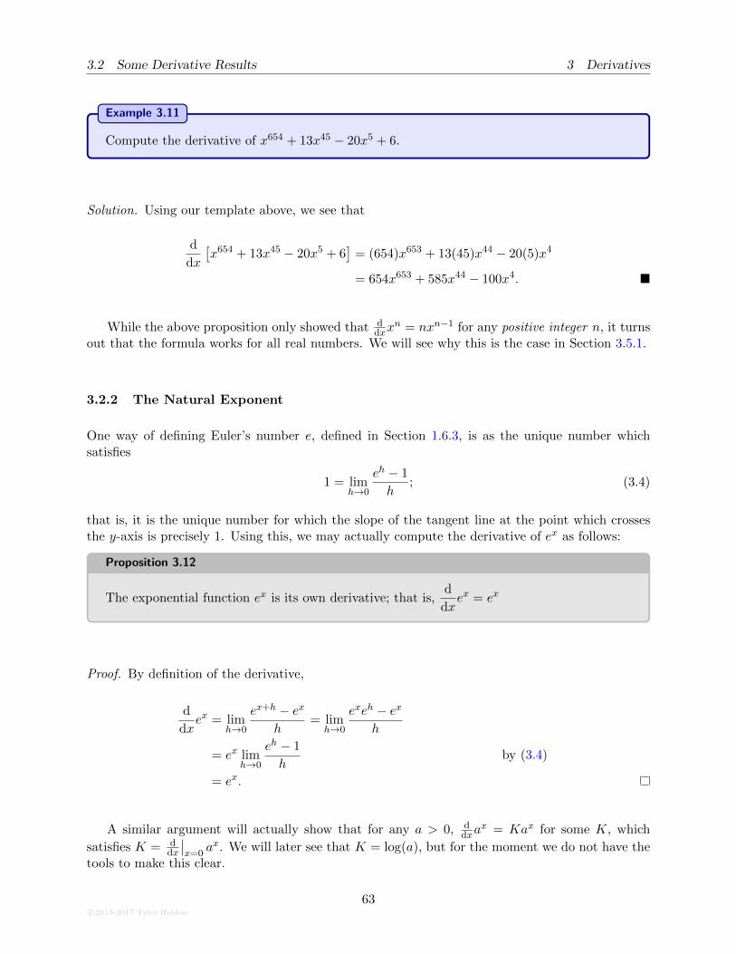
3.2 Some Derivative Results 3 Derivatives
Example 3.11
Compute the derivative of x654 + 13x45 − 20x5 + 6.
Solution. Using our template above, we see that
d
dx
[x654 + 13x45 − 20x5 + 6
]= (654)x653 + 13(45)x44 − 20(5)x4
= 654x653 + 585x44 − 100x4. �
While the above proposition only showed that ddxx
n = nxn−1 for any positive integer n, it turnsout that the formula works for all real numbers. We will see why this is the case in Section 3.5.1.
3.2.2 The Natural Exponent
One way of defining Euler’s number e, defined in Section 1.6.3, is as the unique number whichsatisfies
1 = limh→0
eh − 1
h; (3.4)
that is, it is the unique number for which the slope of the tangent line at the point which crossesthe y-axis is precisely 1. Using this, we may actually compute the derivative of ex as follows:
Proposition 3.12
The exponential function ex is its own derivative; that is,d
dxex = ex
Proof. By definition of the derivative,
d
dxex = lim
h→0
ex+h − exh
= limh→0
exeh − exh
= ex limh→0
eh − 1
hby (3.4)
= ex.
A similar argument will actually show that for any a > 0, ddxa
x = Kax for some K, which
satisfies K = ddx
∣∣x=0
ax. We will later see that K = log(a), but for the moment we do not have thetools to make this clear.
c©2013-2017 Tyler Holden
63
3 Derivatives 3.2 Some Derivative Results
Exercise: Recall that if n is a positive integer, we define n! = n(n− 1)(n− 2) · · · (3)(2). Forexample, 3! = 3× 2 = 6 and 4! = 4× 3× 2 = 24. Consider the function
f(x) = 1 + x+x2
2!+x3
3!+x4
4!+x5
5!+ · · · .
Compute the derivative of f(x). If you are given that derivatives are unique up to additiveconstants, what function must f(x) be?
3.2.3 The Product and Quotient Rule
Computing the derivative of sums of functions was ultimately rather simple. However, it turns outthat computing the derivative of a product is a far more complicated affair.
Theorem 3.13
If f(x) and g(x) are differentiable at c, then f(x)g(x) is differentiable at c and
d
dx
∣∣∣∣x=c
f(x)g(x) = f ′(c)g(c) + g′(c)f(c).
Proof. By the limit definition of the derivative, we have
d
dc
∣∣∣∣c=c
f(c)g(c) = limh→0
f(c+ h)g(c+ h)− f(c)g(c)
h
= limh→0
f(c+ h)g(c+ h) + f(c+ h)g(c)− f(c+ h)g(c)− f(c)g(c)
h
= limh→0
f(c+ h)g(c+ h)− g(c)
h+ g(c)
f(c+ h)− f(c)
h
=
[limh→0
f(c+ h)
] [limh→0
g(c+ h)− g(c)
h
]+ g(c)
[limh→0
f(c+ h)− f(c)
h
]
= f(c)g′(c) + g(c)f ′(c).
Example 3.14
Let f(x) be a differentiable function such that f ′(x) = 1/f(x). Compute ddx [f(x)]2.
Solution. Applying the product rule, we have
d
dx[f(x)]2 = f ′(x)f(x) + f ′(x)f(x) = 2f ′(x)f(x).
Now since we were told that f ′(x) = 1/f(x) we may substitute this to find that
d
dx[f(x)]2 = 2f ′(x)f(x) = 2
f(x)
f(x)= 2. �
64c©2013-2017 Tyler Holden
3.2 Some Derivative Results 3 Derivatives
Exercise: Find a differentiable function that satisfies f ′(x) = [f(x)]−1 as in Example 3.14.
Example 3.15
Let f(x) be differentiable and satisfy f(1) = 1 and f ′(1) = 2. Compute g′(1) where g(x) =f(x)/x.
Solution. We have already seen that ddx
1x = − 1
x2, so the product rule tells us that
d
dxg(x) =
d
dx
[f(x)× 1
x
]= f ′(x)
(1
x
)+ f(x)
(d
dx
1
x
)
=f ′(x)
x+ f(x)
(− 1
x2
)
=f ′(x)
x− f(x)
x2.
If we now substitute x = 1 into this equation we find
g′(1) =f ′(1)
1− f(1)
12=
2
1− 1
1= 2− 1 = 1. �
In fact, there is no reason to limit ourselves to considering the product of only two functions.If f(x), g(x), and h(x) are all differentiable then
d
dxf(x)g(x)h(x) = f ′(x)g(x)h(x) + f(x)g′(x)h(x) + f(x)g(x)h′(x).
The way to see this is to define a new function n(x) = g(x)h(x) so that n′(x) = g′(x)h(x)+g(x)h′(x)and f(x)g(x)h(x) = f(x)n(x). Since the right-hand-side is a product of two functions, the productrule again gives us
d
dxf(x)n(x) = f ′(x)n(x) + f(x)n′(x) = f ′(x)g(x)h(x) + f(x)
[g′(x)h(x) + g(x)h′(x)
]
= f ′(x)g(x)h(x) + f(x)g′(x)h(x) + f(x)g(x)h′(x)
and this process is easily generalized to any number of functions.
Theorem 3.16: The Quotient Rule
If f(x) and g(x) are differentiable at c and g(c) 6= 0 then f(x)/g(x) is differentiable at c and
d
dc
∣∣∣∣x=c
f(x)
g(x)=f ′(c)g(c)− f(c)g′(c)
[g(c)]2.
Example 3.17
Compute the derivative of f(x) =x2 − 2x+ 1
x4 + 4.
c©2013-2017 Tyler Holden
65
3 Derivatives 3.2 Some Derivative Results
Solution. Let us write g(x) = x2 − 2x+ 1 and h(x) = x4 + 4 so that f(x) = g(x)/h(x). We knowthat g′(x) = 2x− 2 and h′(x) = 4x3 so
d
dx
x2 − 2x+ 1
x4 + 4=g′(x)h(x)− g(x)h′(x)
[h(x)]2
=(2x− 2)(x4 + 4)− (4x3)(x2 − 2x+ 1)
[x4 + 4]2
=−2x5 + 6x4 − 4x3 + 8x− 8
[x4 + 4]2�
Example 3.18
Confirm the computation of the derivative of f(x)/x given in Example 3.15.
Solution. Applying the quotient rule to f(x)/x we find that
d
dx
f(x)
x=f ′(x)x−
(d
dxx)f(x)
[x2]
=xf ′(x)− f(x)
x2.
In Example 3.15 we found that
d
dx
f(x)
x=f ′(x)
x− f(x)
x2=xf ′(x)− f(x)
x2
exactly as expected. �
Example 3.19
If g(x) = x/ex, find an expression for g(n)(x).
Solution. Once we have learned the chain rule, this example will be much more easily computedby using the product rule on g(x) = xe−x. For the moment though we must content ourselves withusing the quotient rule. Since we would like to find a general expression for the nth derivative ofg(x), we will start by computing the first few derivatives and see if we can find a pattern. The firstseveral derivatives are as follows:
f ′(x) =ex − xexe2x
=1− xex
f ′′(x) =−ex − (1− x)ex
e2x=−1− 1 + x
ex=−(2− x)
ex
f ′′′(x) =ex − (x− 2)ex
e2x=
1− x+ 2
ex=
3− xex
.
The pattern would suggest that in general,
g(n)(x) =(−1)n−1(n− x)
ex. �
66c©2013-2017 Tyler Holden
3.3 Trigonometric Derivatives 3 Derivatives
3.2.4 Higher Order Derivatives
Differentiating a function f(x) resulted in another function f ′(x). If f ′(x) is itself differentiablethen we can apply the derivative again to find the second derivative f ′′(x). If f ′′(x) is differentiable,we can differentiate a third time to get f ′′′(x), and so on.
When using the prime notation becomes too cumbers on, we let f (n)(x) denote the nth derivativeof f(x). These have important interpretations in both mathematics and science which we shallexplore later. In Leibniz notation, we use the operator d
dx to take subsequent derivatives, hence if
y = f(x) then the first derivative is dydx , while the second, third, and fourth derivatives are
d
dx
dy
dx=
d2y
dx2,
d
dx
d2y
dx2=
d3y
dx3,
d
dx
d3y
dx3=
d4y
dx4
respectively, with the pattern continuing ad infinitum. to
Example 3.20
Compute the second derivative of the function f(x) = 1/x. Determine a formula for the nth
derivative f (n)(x).
Solution. In Example 3.6 we showed that f ′(x) = −1/x2. To compute f ′′(x) we take the derivateof f ′(x) using the quotient rule, and find that
f ′′(x) =d
dx
(− 1
x2
)=
2
x3.
Were we to continue on in this fashion, the higher order derivatives would be computed to be
f ′′′(x) =−6
x4, f (4)(x) =
24
x5, f (5)(x) = −120
x6, . . . .
In general, the n-th derivative of f is given by
f (n)(x) =(−1)nn!
xn+1. �
3.3 Trigonometric Derivatives
We now explore the derivatives of the trigonometric functions sin(x) and cos(x). Since all othertrigonometric functions, such as tan(x) and sec(x), are built from quotients of these two functions,our knowledge of the product and quotient rules will allow us to compute the derivatives of all theremaining fundamental trigonometric functions.
3.3.1 Two Important Limits
The proof of the following two limits requires some geometry and the Squeeze Theorem. They aregood exercises in their own right, but their derivation is beyond the scope of this course.
c©2013-2017 Tyler Holden
67
3 Derivatives 3.3 Trigonometric Derivatives
limθ→0
sin(θ)
θ= 1, lim
θ→0
cos(θ)− 1
θ= 0.
This essentially tells us that sin(θ) and θ converge to zero at approximately the same rate, whilecos(θ)− 1 goes to zero strictly faster than θ. In fact, the above two results may be generalized asfollows: If k 6= 0 is any real number, then
limθ→0
sin(kθ)
kθ= 1, lim
θ→0
cos(kθ)− 1
kθ= 0.
Example 3.21
Determine the limit limx→0
sin(3x)
x.
Solution. The above limit is of the form 0/0 so we may not simply substitute x = 0 into the formula.On the other hand, we only have information on how sin(3x)/3x behaves, and not sin(3x)/x. Oursolution to this should be to manipulate sin(3x)/x into looking like sin(3x)/3x by multiplying anddividing by 3. This gives us
limx→0
sin(3x)
x
3
3= 3 lim
x→0
sin(3x)
3x= 3 �
Example 3.22
Determine the limit limx→0
sin2(4x)
3x2.
Solution. The presence of the sin2(4x) term should not intimidate us as we know how to deal withthe limit of a product. Indeed, our goal should be to rewrite this as
sin2(4x)
16x2=
sin2(4x)
(4x2)=
sin(4x)
4x
sin(4x)
4x.
Since the denominator is only 3x2 as compared to the necessary 16x2, we multiply and divideeverything by 16/3, so that
limx→0
sin2(4x)
3x2
16/3
16/3=
16
3limx→0
sin2(4x)163 3x2
=16
3limx→0
sin2(4x)
16x2=
16
3
[limx→0
sin(4x)
4x
] [limx→0
sin(4x)
4x
]
=16
3. �
68c©2013-2017 Tyler Holden
3.3 Trigonometric Derivatives 3 Derivatives
3.3.2 Differentiating Sine and Cosine
To differentiate sine and cosine, we will use the two limits above as well as the angle sum identities:
sin(x± y) = sin(x) cos(y)± cos(x) sin(y), cos(x± y) = cos(x) cos(y)∓ sin(x) sin(y).
Theorem 3.23
The functions sin(x) and cos(x) are everywhere differentiable, and in particular
d
dxsin(x) = cos(x),
d
dxcos(x) = − sin(x).
Proof. We will demonstrate the proof for the derivative of sin(x) and leave the proof for cos(x) asan exercise for the student. Applying the definition of the derivative we have
d
dxsin(x) = lim
h→0
sin(x+ h)− sin(x)
h
= limh→0
sin(x) cos(h) + cos(x) sin(h)− sin(x)
hby the double angle identity
= limh→0
sin(x)cos(h)− 1
h+ cos(x)
sin(h)
h
= sin(x)
[limh→0
cos(h)− 1
h
]
︸ ︷︷ ︸=0
+ cos(x)
[limh→0
sin(h)
h
]
︸ ︷︷ ︸=1
by the limit laws
= cos(x).
Example 3.24
Using the quotient rule, compute the derivative of tan(x).
Solution. Since tan(x) = sin(x)/ cos(x) we can apply the quotient rule to find
d
dxtan(x) =
[d
dx sin(x)]
cos(x)− sin(x)[
ddx cos(x)
]
cos2(x)
=cos2(x) + sin2(x)
cos2(x)=
1
cos2(x)
= sec2(x). �
Computing the remaining trigonometric derivatives is an excellent exercise in the use of thequotient rule, but we shall provide here a table of the trigonometric derivatives:
As a general rule, many of these identities are not worth remembering. Instead, the studentshould focus on how to derive these relationships using the quotient rule, so that the formulae canbe called upon when needed.
c©2013-2017 Tyler Holden
69
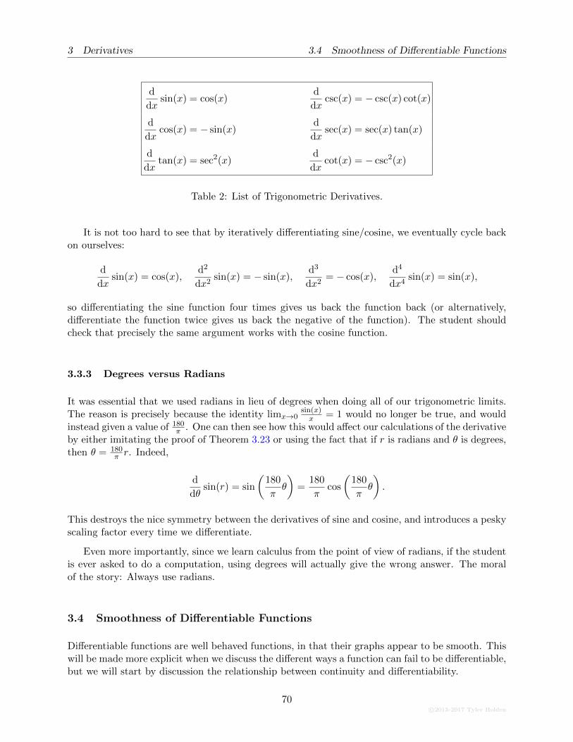
3 Derivatives 3.4 Smoothness of Differentiable Functions
d
dxsin(x) = cos(x)
d
dxcsc(x) = − csc(x) cot(x)
d
dxcos(x) = − sin(x)
d
dxsec(x) = sec(x) tan(x)
d
dxtan(x) = sec2(x)
d
dxcot(x) = − csc2(x)
Table 2: List of Trigonometric Derivatives.
It is not too hard to see that by iteratively differentiating sine/cosine, we eventually cycle backon ourselves:
d
dxsin(x) = cos(x),
d2
dx2sin(x) = − sin(x),
d3
dx2= − cos(x),
d4
dx4sin(x) = sin(x),
so differentiating the sine function four times gives us back the function back (or alternatively,differentiate the function twice gives us back the negative of the function). The student shouldcheck that precisely the same argument works with the cosine function.
3.3.3 Degrees versus Radians
It was essential that we used radians in lieu of degrees when doing all of our trigonometric limits.The reason is precisely because the identity limx→0
sin(x)x = 1 would no longer be true, and would
instead given a value of 180π . One can then see how this would affect our calculations of the derivative
by either imitating the proof of Theorem 3.23 or using the fact that if r is radians and θ is degrees,then θ = 180
π r. Indeed,
d
dθsin(r) = sin
(180
πθ
)=
180
πcos
(180
πθ
).
This destroys the nice symmetry between the derivatives of sine and cosine, and introduces a peskyscaling factor every time we differentiate.
Even more importantly, since we learn calculus from the point of view of radians, if the studentis ever asked to do a computation, using degrees will actually give the wrong answer. The moralof the story: Always use radians.
3.4 Smoothness of Differentiable Functions
Differentiable functions are well behaved functions, in that their graphs appear to be smooth. Thiswill be made more explicit when we discuss the different ways a function can fail to be differentiable,but we will start by discussion the relationship between continuity and differentiability.
70c©2013-2017 Tyler Holden
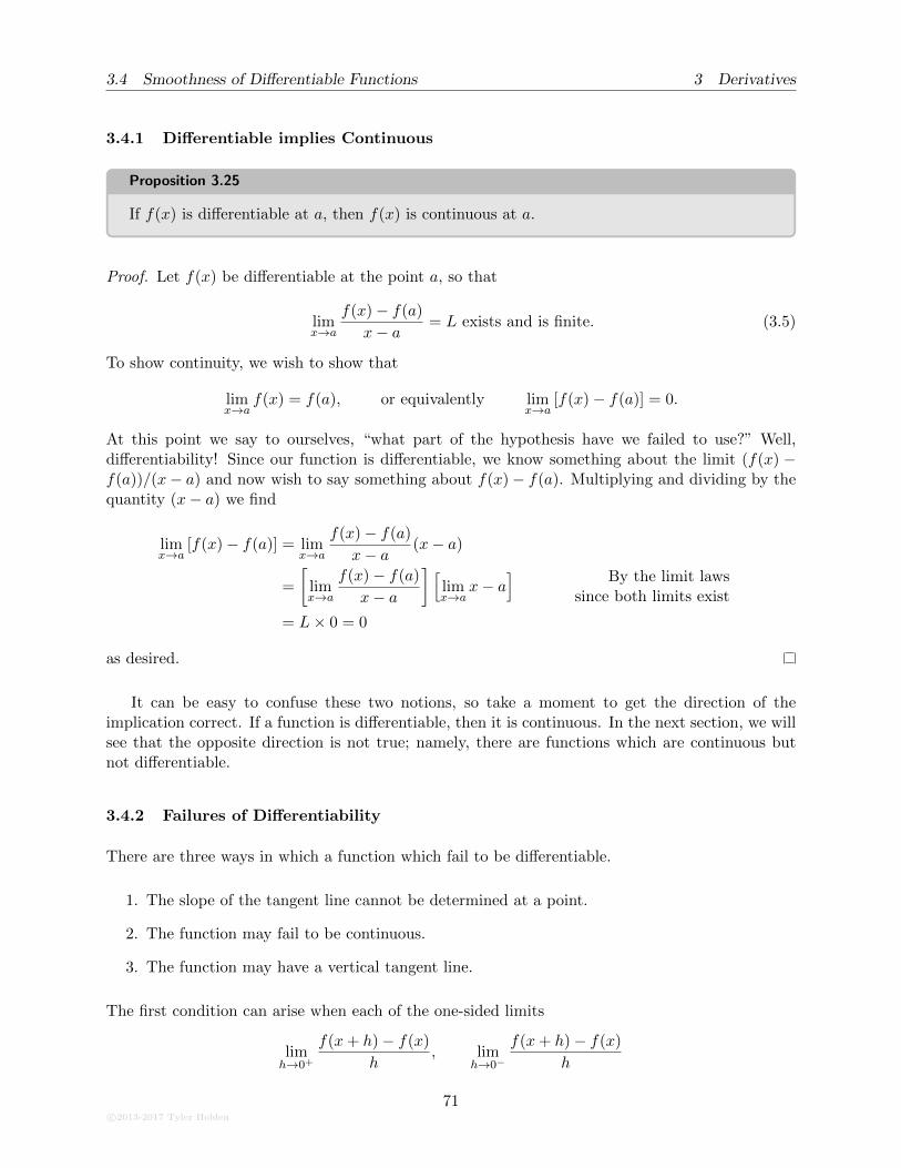
3.4 Smoothness of Differentiable Functions 3 Derivatives
3.4.1 Differentiable implies Continuous
Proposition 3.25
If f(x) is differentiable at a, then f(x) is continuous at a.
Proof. Let f(x) be differentiable at the point a, so that
limx→a
f(x)− f(a)
x− a = L exists and is finite. (3.5)
To show continuity, we wish to show that
limx→a
f(x) = f(a), or equivalently limx→a
[f(x)− f(a)] = 0.
At this point we say to ourselves, “what part of the hypothesis have we failed to use?” Well,differentiability! Since our function is differentiable, we know something about the limit (f(x) −f(a))/(x− a) and now wish to say something about f(x)− f(a). Multiplying and dividing by thequantity (x− a) we find
limx→a
[f(x)− f(a)] = limx→a
f(x)− f(a)
x− a (x− a)
=
[limx→a
f(x)− f(a)
x− a
] [limx→a
x− a] By the limit laws
since both limits exist
= L× 0 = 0
as desired.
It can be easy to confuse these two notions, so take a moment to get the direction of theimplication correct. If a function is differentiable, then it is continuous. In the next section, we willsee that the opposite direction is not true; namely, there are functions which are continuous butnot differentiable.
3.4.2 Failures of Differentiability
There are three ways in which a function which fail to be differentiable.
1. The slope of the tangent line cannot be determined at a point.
2. The function may fail to be continuous.
3. The function may have a vertical tangent line.
The first condition can arise when each of the one-sided limits
limh→0+
f(x+ h)− f(x)
h, lim
h→0−
f(x+ h)− f(x)
h
c©2013-2017 Tyler Holden
71
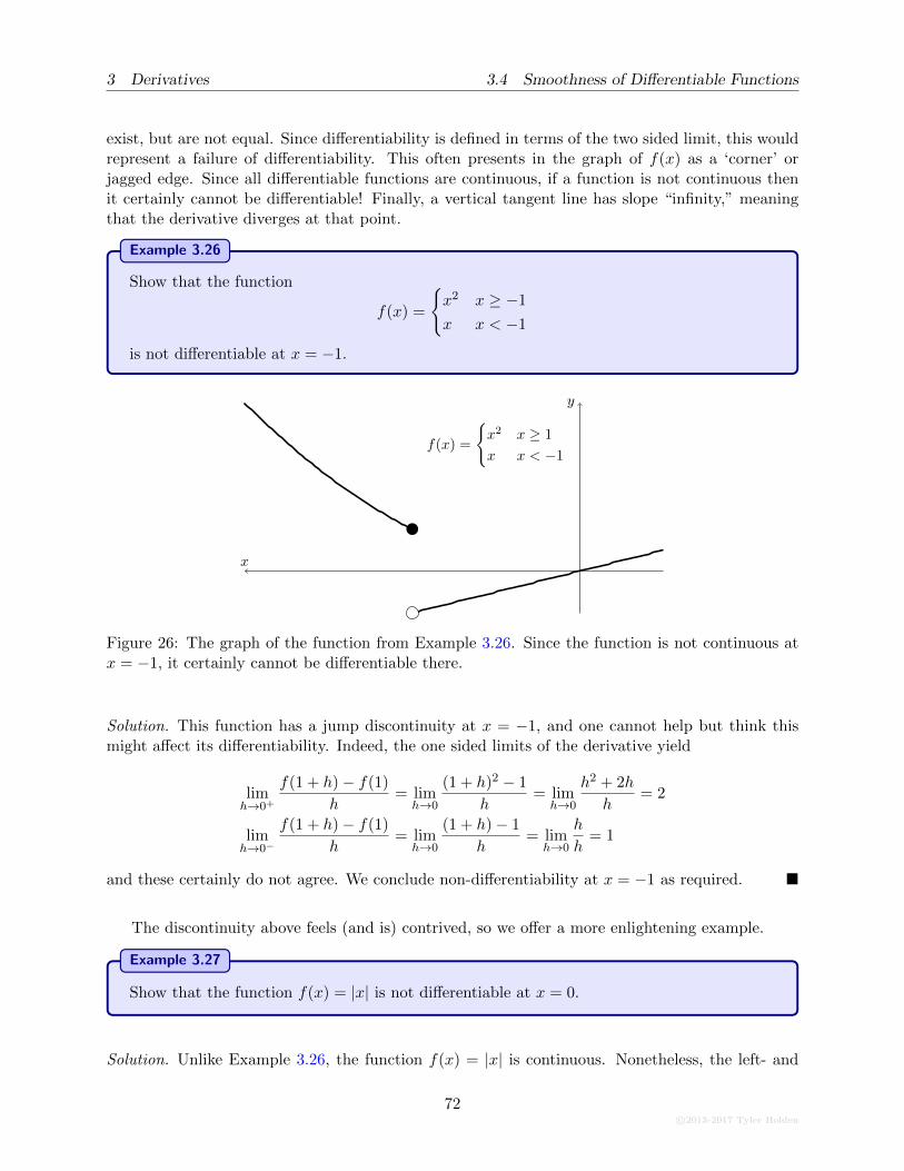
3 Derivatives 3.4 Smoothness of Differentiable Functions
exist, but are not equal. Since differentiability is defined in terms of the two sided limit, this wouldrepresent a failure of differentiability. This often presents in the graph of f(x) as a ‘corner’ orjagged edge. Since all differentiable functions are continuous, if a function is not continuous thenit certainly cannot be differentiable! Finally, a vertical tangent line has slope “infinity,” meaningthat the derivative diverges at that point.
Example 3.26
Show that the function
f(x) =
{x2 x ≥ −1
x x < −1
is not differentiable at x = −1.
x
y
f(x) =
{x2 x ≥ 1
x x < −1
Figure 26: The graph of the function from Example 3.26. Since the function is not continuous atx = −1, it certainly cannot be differentiable there.
Solution. This function has a jump discontinuity at x = −1, and one cannot help but think thismight affect its differentiability. Indeed, the one sided limits of the derivative yield
limh→0+
f(1 + h)− f(1)
h= lim
h→0
(1 + h)2 − 1
h= lim
h→0
h2 + 2h
h= 2
limh→0−
f(1 + h)− f(1)
h= lim
h→0
(1 + h)− 1
h= lim
h→0
h
h= 1
and these certainly do not agree. We conclude non-differentiability at x = −1 as required. �
The discontinuity above feels (and is) contrived, so we offer a more enlightening example.
Example 3.27
Show that the function f(x) = |x| is not differentiable at x = 0.
Solution. Unlike Example 3.26, the function f(x) = |x| is continuous. Nonetheless, the left- and
72c©2013-2017 Tyler Holden
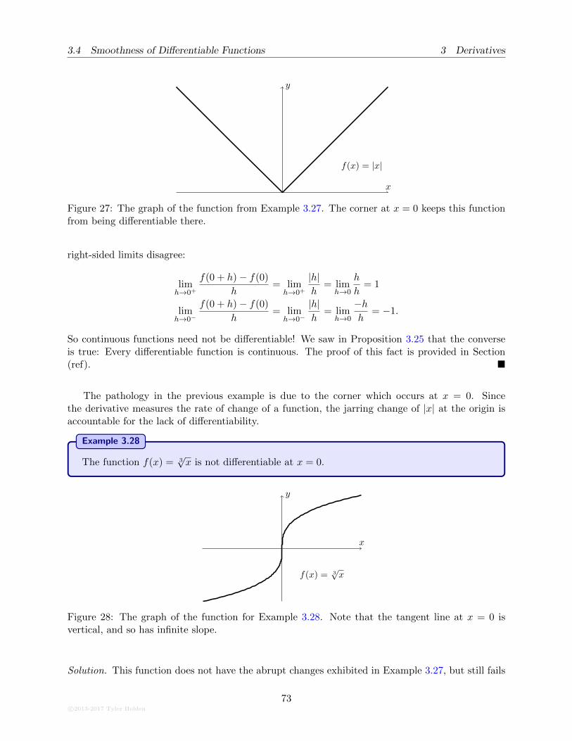
3.4 Smoothness of Differentiable Functions 3 Derivatives
x
y
f(x) = |x|
Figure 27: The graph of the function from Example 3.27. The corner at x = 0 keeps this functionfrom being differentiable there.
right-sided limits disagree:
limh→0+
f(0 + h)− f(0)
h= lim
h→0+
|h|h
= limh→0
h
h= 1
limh→0−
f(0 + h)− f(0)
h= lim
h→0−
|h|h
= limh→0
−hh
= −1.
So continuous functions need not be differentiable! We saw in Proposition 3.25 that the converseis true: Every differentiable function is continuous. The proof of this fact is provided in Section(ref). �
The pathology in the previous example is due to the corner which occurs at x = 0. Sincethe derivative measures the rate of change of a function, the jarring change of |x| at the origin isaccountable for the lack of differentiability.
Example 3.28
The function f(x) = 3√x is not differentiable at x = 0.
x
y
f(x) = 3√x
Figure 28: The graph of the function for Example 3.28. Note that the tangent line at x = 0 isvertical, and so has infinite slope.
Solution. This function does not have the abrupt changes exhibited in Example 3.27, but still fails
c©2013-2017 Tyler Holden
73
3 Derivatives 3.5 Chains and Inverses
to be differentiable at 0. Our one-sided limits give
limh→0+
f(0 + h)− f(0)
h= lim
h→0
3√h
h= lim
h→0
1
h2/3=∞.
This implies there is a sense in which the derivative exists, it is just that the tangent line has infiniteslope; that is, the tangent line is vertical. As we would prefer to avoid having the incorporation ofinfinities into our formalism, we say that f(x) is not differentiable at 0 all the same. �
3.5 Chains and Inverses
We have seen how to take the derivatives of sums, products, and quotients of functions. The onlymajor operation left is to look at function composition. Interestingly, determine how to differentiatea composition will also give us access to the derivative of inverse functions.
3.5.1 The Chain Rule
Why are we interested in differentiating compositions? Let’s say that you’re a weatherperson andyou want to determine the outside temperature over the course of the day. You realize that thetemperature H depends on the amount of sunshine s, and they are related through a function H =f(s). This makes perfect sense, and you can even use calculus to determine dH
ds , the instantaneousrate of change of temperature with respect to sunshine.
But maybe you find it difficult to measure the amount of sunshine directly. Instead, you realizethat sunshine itself is a function of time t; that is, you can write s = g(t) for some function g. Thisallows you to determine ds
dt , the instantaneous rate of sunshine with respect to time.
The composition H = f(s) = f(g(t)) now tells you how the temperature depends on time.However, to differentiate this function you need to be able to differentiate the composition f ◦ g.It seems like you should be able to do this; after all, you know how temperature changes withsunshine, and how sunshine changes with time:
time −→ sunshine −→ temperature.
Here, sunshine just acts as an intermediary for getting from time to temperature, and we can writeT = f(s) = f(g(t)). This is our goal.
Theorem 3.29: Chain Rule
If f(x) and g(x) are functions such that g(x) is differentiable at c and f(x) is differentiableat g(c), then the composition f ◦ g is differentiable at c and (f ◦ g)′(c) = f ′(g(c))g′(c).In Leibniz notation, if w = f(y) and y = g(x) then
dw
dx
∣∣∣∣a
=dw
dy
∣∣∣∣g(a)
dy
dx
∣∣∣∣a
. (3.6)
74c©2013-2017 Tyler Holden
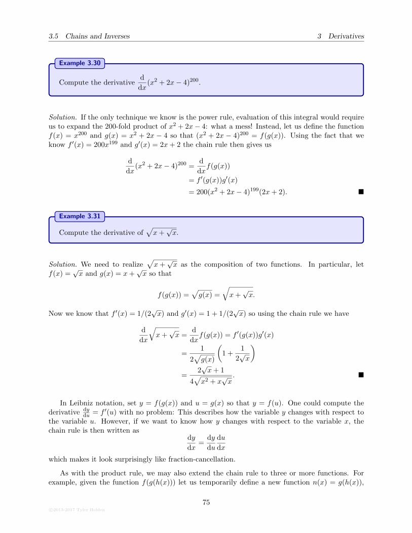
3.5 Chains and Inverses 3 Derivatives
Example 3.30
Compute the derivatived
dx(x2 + 2x− 4)200.
Solution. If the only technique we know is the power rule, evaluation of this integral would requireus to expand the 200-fold product of x2 + 2x− 4: what a mess! Instead, let us define the functionf(x) = x200 and g(x) = x2 + 2x − 4 so that (x2 + 2x − 4)200 = f(g(x)). Using the fact that weknow f ′(x) = 200x199 and g′(x) = 2x+ 2 the chain rule then gives us
d
dx(x2 + 2x− 4)200 =
d
dxf(g(x))
= f ′(g(x))g′(x)
= 200(x2 + 2x− 4)199(2x+ 2). �
Example 3.31
Compute the derivative of√x+√x.
Solution. We need to realize√x+√x as the composition of two functions. In particular, let
f(x) =√x and g(x) = x+
√x so that
f(g(x)) =√g(x) =
√x+√x.
Now we know that f ′(x) = 1/(2√x) and g′(x) = 1 + 1/(2
√x) so using the chain rule we have
d
dx
√x+√x =
d
dxf(g(x)) = f ′(g(x))g′(x)
=1
2√g(x)
(1 +
1
2√x
)
=2√x+ 1
4√x2 + x
√x. �
In Leibniz notation, set y = f(g(x)) and u = g(x) so that y = f(u). One could compute thederivative dy
du = f ′(u) with no problem: This describes how the variable y changes with respect tothe variable u. However, if we want to know how y changes with respect to the variable x, thechain rule is then written as
dy
dx=
dy
du
du
dx
which makes it look surprisingly like fraction-cancellation.
As with the product rule, we may also extend the chain rule to three or more functions. Forexample, given the function f(g(h(x))) let us temporarily define a new function n(x) = g(h(x)),
c©2013-2017 Tyler Holden
75
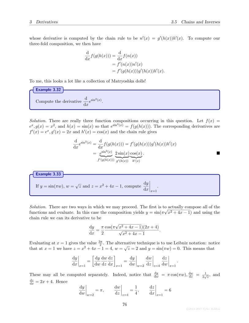
3 Derivatives 3.5 Chains and Inverses
whose derivative is computed by the chain rule to be n′(x) = g′(h(x))h′(x). To compute ourthree-fold composition, we then have
d
dxf(g(h(x))) =
d
dxf(n(x))
= f ′(n(x))n′(x)
= f ′(g(h(x)))g′(h(x))h′(x).
To me, this looks a lot like a collection of Matryoshka dolls!
Example 3.32
Compute the derivatived
dxesin2(x).
Solution. There are really three function compositions occurring in this question. Let f(x) =ex, g(x) = x2, and h(x) = sin(x) so that esin2(x) = f(g(h(x))). The corresponding derivatives aref ′(x) = ex, g′(x) = 2x and h′(x) = cos(x) and the chain rule gives
d
dxesin2(x) =
d
dxf(g(h(x))) = f ′(g(h(x)))g′(h(x))h′(x)
= esin2(x)︸ ︷︷ ︸f ′(g(h(x)))
2 sin(x)︸ ︷︷ ︸g′(h(x))
cos(x)︸ ︷︷ ︸h′(x)
. �
Example 3.33
If y = sin(πw), w =√z and z = x2 + 4x− 1, compute
dy
dx
∣∣∣∣x=1
.
Solution. There are two ways in which we may proceed. The first is to actually compose all of thefunctions and evaluate. In this case the composition yields y = sin(π
√x2 + 4x− 1) and using the
chain rule we can its derivative to be
dy
dx=π
2
cos(π√x2 + 4x− 1)(2x+ 4)√x2 + 4x− 1
.
Evaluating at x = 1 gives the value 3π2 . The alternative technique is to use Leibniz notation: notice
that at x = 1 we have z = x2 + 4x− 1 = 4, w =√z = 2 and y = sin(πw) = 0. This means that
dy
dx
∣∣∣∣x=1
=
[dy
dw
dw
dz
dz
dx
]
x=1
=dy
dw
∣∣∣∣w=2
dw
dz
∣∣∣∣z=4
dz
dw
∣∣∣∣x=1
.
These may all be computed separately. Indeed, notice that dydw = π cos(πw), dw
dz = 12√z, and
dzdx = 2x+ 4. Hence
dy
dw
∣∣∣∣w=2
= π,dw
dz
∣∣∣∣z=4
=1
4,
dz
dx
∣∣∣∣x=1
= 6
76c©2013-2017 Tyler Holden
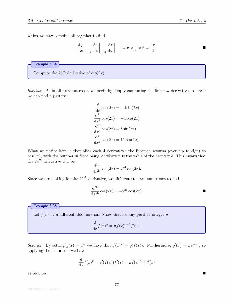
3.5 Chains and Inverses 3 Derivatives
which we may combine all together to find
dy
dw
∣∣∣∣w=2
dw
dz
∣∣∣∣z=4
dz
dw
∣∣∣∣x=1
= π × 1
4× 6 =
3π
2. �
Example 3.34
Compute the 26th derivative of cos(2x).
Solution. As in all previous cases, we begin by simply computing the first few derivatives to see ifwe can find a pattern:
d
dxcos(2x) = −2 sin(2x)
d2
dx2cos(2x) = −4 cos(2x)
d3
dx3cos(2x) = 8 sin(2x)
d4
dx4cos(2x) = 16 cos(2x).
What we notice here is that after each 4 derivatives the function returns (even up to sign) tocos(2x), with the number in front being 2n where n is the value of the derivative. This means thatthe 24th derivative will be
d24
dx24cos(2x) = 224 cos(2x).
Since we are looking for the 26th derivative, we differentiate two more times to find
d26
dx26cos(2x) = −226 cos(2x). �
Example 3.35
Let f(x) be a differentiable function. Show that for any positive integer n
d
dxf(x)n = nf(x)n−1f ′(x).
Solution. By setting g(x) = xn we have that f(x)n = g(f(x)). Furthermore, g′(x) = nxn−1, soapplying the chain rule we have
d
dxf(x)n = g′(f(x))f ′(x) = nf(x)n−1f ′(x)
as required. �
c©2013-2017 Tyler Holden
77

3 Derivatives 3.5 Chains and Inverses
Example 3.36
Denote by f◦n(x) the n-fold composition of f . For example, f◦3(x) = f(f(f(x))). Assumingthat f(1) = 1 and f ′(1) = 2 find the derivative of f◦n evaluated at x = 1.
Solution. This is just a repeated exercise of the chain rule requiring a small bit of trickery. First,we notice that since f(1) = 1 then no matter how many times we compose by f , we will alwaysget 1. More explicitly, notice that f(f(1)) = f(1) = 1, and in general f◦n(1) = 1. For the sake ofintuition, let us try this when n = 3. Notice in this case that
(f◦3)′(x) = f ′(f(f(x))) · f ′(f(x)) · f ′(x)
so that
(f◦3)′(1) = f ′(f(f(1))) · f ′(f(1) · f ′(1) = f ′(1) · f ′(1) · f ′(1) =[f ′(1)
]3= 8.
In fact, precisely the same procedure will work for general n, and we get
(f◦n)′(x) = f ′(f◦(n−1)(x))f ′(f◦(n−2)(x)) · · · f ′(f(x))f ′(x) =n−1∏
i=0
f ′(f◦i(x))
where f◦0 = x. Hence we get
(f◦n)′(1) = f ′(1) · · · f ′(1)︸ ︷︷ ︸n−times
= 2n. �
Just as we were able to use the product rule to extend the power rule from n ∈ N to n ∈ Z, wecan use the product rule to tell us something about inverse functions (we will discuss this more ina subsequent section).
3.5.2 Derivatives of Inverse Functions
Theorem 3.37: Inverse Function Theorem
Let f(x) be differentiable at the point c with f ′(x) continuous at c. If f ′(c) 6= 0, then there isan interval I containing c on which f is invertible. Moreover, the inverse f−1 is differentiablewith continuous derivative, and satisfies the formula
(f−1
)′(x) =
1
f ′(f−1(x)). (3.7)
The majority of this theorem is beyond our abilities, but deriving Equation (3.7) is not toodifficult. Let us begin by assuming that we have been given f−1 and we know that it is differentiable.By definition of the inverse function we have f(f−1(x)) = x for all x in the range of f . Differentiatingboth sides (applying the chain rule to the composition) we then get
1 =d
dxf(f−1(x)) = f ′(f−1(x))(f−1)′(x).
78c©2013-2017 Tyler Holden
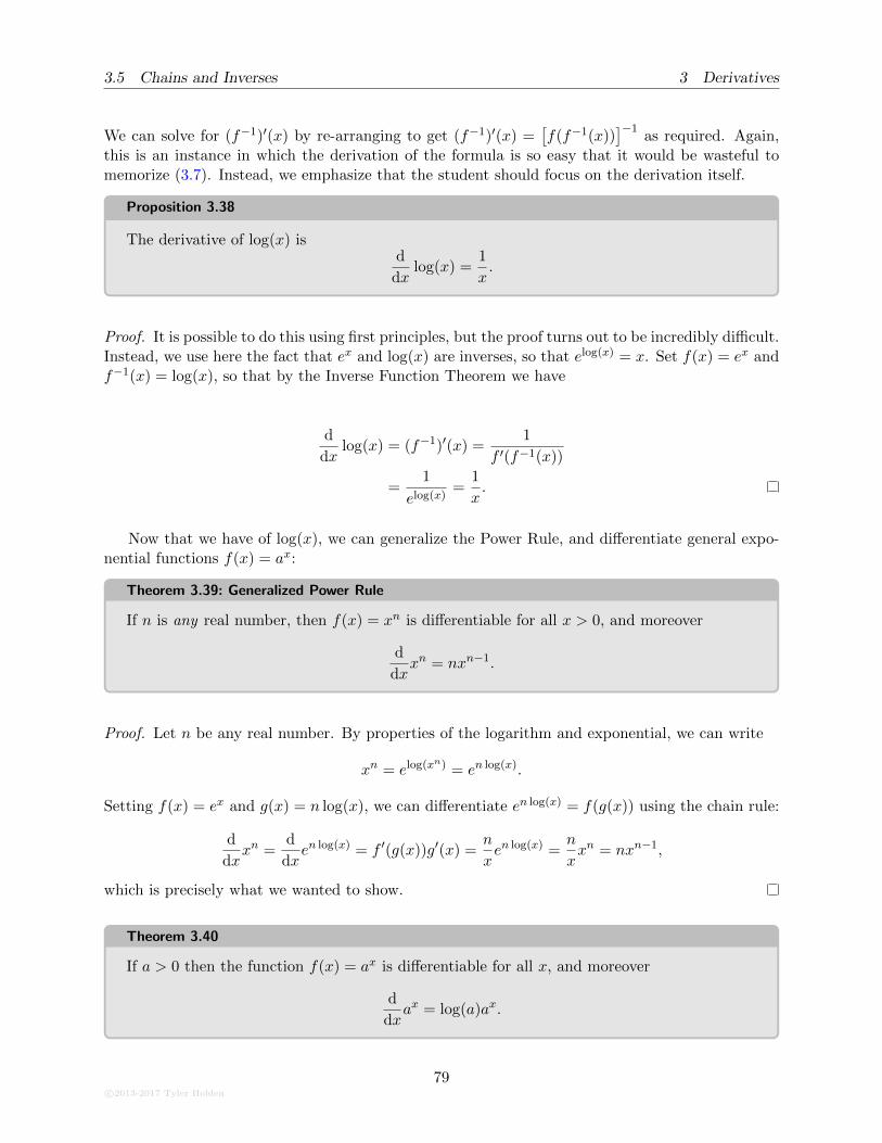
3.5 Chains and Inverses 3 Derivatives
We can solve for (f−1)′(x) by re-arranging to get (f−1)′(x) =[f(f−1(x))
]−1as required. Again,
this is an instance in which the derivation of the formula is so easy that it would be wasteful tomemorize (3.7). Instead, we emphasize that the student should focus on the derivation itself.
Proposition 3.38
The derivative of log(x) isd
dxlog(x) =
1
x.
Proof. It is possible to do this using first principles, but the proof turns out to be incredibly difficult.Instead, we use here the fact that ex and log(x) are inverses, so that elog(x) = x. Set f(x) = ex andf−1(x) = log(x), so that by the Inverse Function Theorem we have
d
dxlog(x) = (f−1)′(x) =
1
f ′(f−1(x))
=1
elog(x)=
1
x.
Now that we have of log(x), we can generalize the Power Rule, and differentiate general expo-nential functions f(x) = ax:
Theorem 3.39: Generalized Power Rule
If n is any real number, then f(x) = xn is differentiable for all x > 0, and moreover
d
dxxn = nxn−1.
Proof. Let n be any real number. By properties of the logarithm and exponential, we can write
xn = elog(xn) = en log(x).
Setting f(x) = ex and g(x) = n log(x), we can differentiate en log(x) = f(g(x)) using the chain rule:
d
dxxn =
d
dxen log(x) = f ′(g(x))g′(x) =
n
xen log(x) =
n
xxn = nxn−1,
which is precisely what we wanted to show.
Theorem 3.40
If a > 0 then the function f(x) = ax is differentiable for all x, and moreover
d
dxax = log(a)ax.
c©2013-2017 Tyler Holden
79
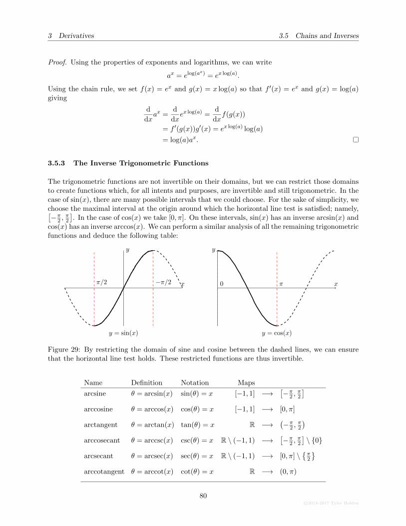
3 Derivatives 3.5 Chains and Inverses
Proof. Using the properties of exponents and logarithms, we can write
ax = elog(ax) = ex log(a).
Using the chain rule, we set f(x) = ex and g(x) = x log(a) so that f ′(x) = ex and g(x) = log(a)giving
d
dxax =
d
dxex log(a) =
d
dxf(g(x))
= f ′(g(x))g′(x) = ex log(a) log(a)
= log(a)ax.
3.5.3 The Inverse Trigonometric Functions
The trigonometric functions are not invertible on their domains, but we can restrict those domainsto create functions which, for all intents and purposes, are invertible and still trigonometric. In thecase of sin(x), there are many possible intervals that we could choose. For the sake of simplicity, wechoose the maximal interval at the origin around which the horizontal line test is satisfied; namely,[−π
2 ,π2
]. In the case of cos(x) we take [0, π]. On these intervals, sin(x) has an inverse arcsin(x) and
cos(x) has an inverse arccos(x). We can perform a similar analysis of all the remaining trigonometricfunctions and deduce the following table:
x
y
π/2 −π/2
y = sin(x)
x
y
0 π
y = cos(x)
Figure 29: By restricting the domain of sine and cosine between the dashed lines, we can ensurethat the horizontal line test holds. These restricted functions are thus invertible.
Name Definition Notation Maps
arcsine θ = arcsin(x) sin(θ) = x [−1, 1] −→[−π
2 ,π2
]
arccosine θ = arccos(x) cos(θ) = x [−1, 1] −→ [0, π]
arctangent θ = arctan(x) tan(θ) = x R −→(−π
2 ,π2
)
arccosecant θ = arccsc(x) csc(θ) = x R \ (−1, 1) −→[−π
2 ,π2
]\ {0}
arcsecant θ = arcsec(x) sec(θ) = x R \ (−1, 1) −→ [0, π] \{π2
}
arccotangent θ = arccot(x) cot(θ) = x R −→ (0, π)
80c©2013-2017 Tyler Holden
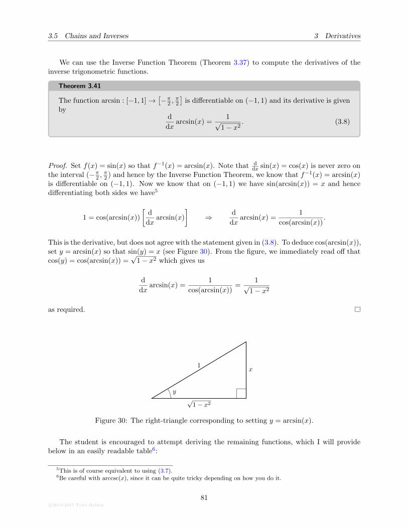
3.5 Chains and Inverses 3 Derivatives
We can use the Inverse Function Theorem (Theorem 3.37) to compute the derivatives of theinverse trigonometric functions.
Theorem 3.41
The function arcsin : [−1, 1]→[−π
2 ,π2
]is differentiable on (−1, 1) and its derivative is given
byd
dxarcsin(x) =
1√1− x2
. (3.8)
Proof. Set f(x) = sin(x) so that f−1(x) = arcsin(x). Note that ddx sin(x) = cos(x) is never zero on
the interval (−π2 ,
π2 ) and hence by the Inverse Function Theorem, we know that f−1(x) = arcsin(x)
is differentiable on (−1, 1). Now we know that on (−1, 1) we have sin(arcsin(x)) = x and hencedifferentiating both sides we have5
1 = cos(arcsin(x))
[d
dxarcsin(x)
]⇒ d
dxarcsin(x) =
1
cos(arcsin(x)).
This is the derivative, but does not agree with the statement given in (3.8). To deduce cos(arcsin(x)),set y = arcsin(x) so that sin(y) = x (see Figure 30). From the figure, we immediately read off thatcos(y) = cos(arcsin(x)) =
√1− x2 which gives us
d
dxarcsin(x) =
1
cos(arcsin(x))=
1√1− x2
as required.
√1− x2
x1
y
Figure 30: The right-triangle corresponding to setting y = arcsin(x).
The student is encouraged to attempt deriving the remaining functions, which I will providebelow in an easily readable table6:
5This is of course equivalent to using (3.7).6Be careful with arccsc(x), since it can be quite tricky depending on how you do it.
c©2013-2017 Tyler Holden
81

3 Derivatives 3.5 Chains and Inverses
d
dxarcsin(x) =
1√1− x2
d
dxarccsc(x) = − 1
|x|√x2 − 1
d
dxarccos(x) = − 1√
1− x2
d
dxarcsec(x) =
1
|x|√x2 − 1
d
dxarctan(x) =
1
1 + x2
d
dxarccot(x) = − 1
1 + x2.
3.5.4 Logarithmic Differentiation
One of the great things about logarithms is there is a sense in which they decrease the complexityof an operation. For example, we often think of addition as being easier than multiplication, andmultiplication being easier than exponents:
log(xy) = log(x) + log(y), log(xy) = y log x.
At the cost of introducing a logarithm, we are able to convert product to sums, and powers toproducts! Since the logarithm is not very hard to differentiate, this does not seem like such aterrible cost.
This idea in general is known as logarithmic differentiation. Where it can be particularly usefulis when we have a product/quotient of many objects which are individually simple to differentiate,but which will become complicated when nested with the product rule. For example, given acollection of functions f1(x), . . . , fn(x) and g1(x), . . . , gm(x), notice that we can write
log
[f1(x) · · · fn(x)
g1(x) · · · gm(x)
]= log f1(x) + · · ·+ log fn(x)− log g1(x)− · · · − log gm(x).
Hence implicit differentiation yields
d
dx
f1(x) · · · fn(x)
g1(x) · · · gm(x)=f1(x) · · · fn(x)
g1(x) · · · gm(x)
d
dx[log f1(x) + · · ·+ log fn(x)− log g1(x)− · · · − log gm(x)]
=f1(x) · · · fn(x)
g1(x) · · · gm(x)
[f ′1(x)
f1(x)+ · · ·+ f ′n(x)
fn(x)− g′1(x)
g1(x)− · · · − g′m(x)
gm(x)
]
Example 3.42
Compute the derivative of f(x) =(x− 1)2(x2 + 2)
√x
x4 + 5.
Solution. This would be an absolute nightmare to compute using the quotient rule, so instead weuse logarithm differentiation. Taking the logarithm of both sides yields:
log f(x) = 2 log(x− 1) + log(x2 + 2) +1
2log(x)− log(x4 + 5).
82c©2013-2017 Tyler Holden
4 Applications of Derivatives
Differentiating implicitly gives
f ′(x) = f(x)d
dx
[2 log(x− 1) + log(x2 + 2) +
1
2log(x)− log(x4 + 5)
]
=(x− 1)2(x3 + 2)
√x
x4 + 5
[2
x− 1+
2x
x2 + 2+
1
2x− 4x3
x4 + 5
]. �
This takes care of converting products to sums, but now what about powers to products? Giventwo functions f(x) and g(x), let’s try to differentiate f(x)g(x). The problem here is that neitherthe power rule, nor the rules for differentiating exponents can apply (in both of those cases, thefunction should only occur in the power or the base, but not both). To deal with this, we sety = f(x)g(x) so that log y = g(x) log f(x). We can now differentiate implicitly:
1
y
dy
dx= g′(x) log f(x) + g(x)
f ′(x)
f(x)
which we may then solve for dydx to get
dy
dx= f(x)g(x)
[g′(x) log f(x) + g(x)
f ′(x)
f(x)
]. (3.9)
Like many of the formulae that we’ve derived, Equation (3.9) is not worth remembering on its own.Rather, what is important is remembering how this derivation was performed so that it can berepeated when necessary.
Example 3.43
Compute the derivative of xsin(x).
Solution. Setting y = xsin(x) we have log y = sin(x) log x. Differentiating implicitly we get
1
y
dy
dx= cos(x) log(x) +
sin(x)
x
which we may solve for dydx to get
dy
dx= xsin(x)
[cos(x) log(x) +
sin(x)
x
]. �
4 Applications of Derivatives
We have developed numerous hammers, and the time has come to start looking for nails. The nextseveral section will discuss how we can apply derivatives to solve applied problems.
c©2013-2017 Tyler Holden
83
4 Applications of Derivatives 4.1 Rates of Change
4.1 Rates of Change
We already saw at the beginning of this section how derivatives can be used to deduce the instan-taneous rate of change of one quantity with respect to another. The power of this is that it allowsus to take boring, static relationships, and differentiate them to discover the dynamic interplaybetween variables.
Example 4.1
The volume of a sphere of radius r is V = 43πr
3. Determine how the volume changes as r isallowed to vary.
Solution. All we need to do is differentiate the given expression with respect to r to find that
dV
dr= 4πr2.
This says that the rate of change of volume V with respect to the radius r is 4πr2. As an example,this means that doubling the radius of a sphere will quadruple its volume, while tripling the radiuswill increase the volume 9-fold. �
One of the more utilized relationships is that of position, velocity, acceleration, jerk, etc. If p(t)describes the position of an object with respect to time, then p′(t) is its velocity and p′′(t) is itsacceleration with respect to time. This can be used to model physical situations which can thenbe solved by mathematical methods:
4.1.1 Gravity
Example 4.2
Consider a child standing on the surface of the earth. If the child has a ball of mass m and,at time t = 0, throws the ball from an initial height y0 with an initial velocity v0, describethe trajectory of the ball as a function of time.
Solution. Here we exploit Newton’s Second Law, which say that the net force Fnet exerted on abody is equal to the object’s inertial mass times its acceleration; that is, Fnet = ma. In our case, weshall ignore air-friction and assume that the force of gravity is a constant, denoted by g. A quicklook at Figure 31 shows us that the net force acting on the ball is F = −mg, where the negativesign is included to indicate that the force of gravity is acting in the opposite direction of initialmotion. Newton’s second law then implies that
F = ma = −mg.
Since the non-zero mass is present on either side of the equation, we may cancel it to deduce thata = −g. But we mentioned earlier that if y is the ball’s vertical displacement, then its acceleration
84c©2013-2017 Tyler Holden
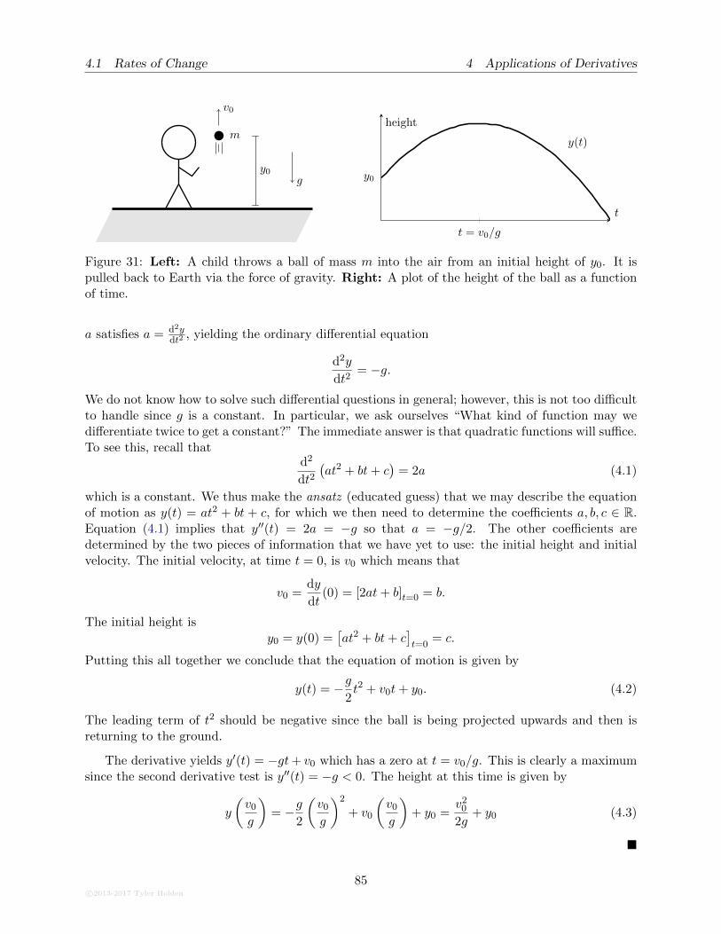
4.1 Rates of Change 4 Applications of Derivatives
m
y0
v0
g
t = v0/g
y0
y(t)
t
height
Figure 31: Left: A child throws a ball of mass m into the air from an initial height of y0. It ispulled back to Earth via the force of gravity. Right: A plot of the height of the ball as a functionof time.
a satisfies a = d2ydt2
, yielding the ordinary differential equation
d2y
dt2= −g.
We do not know how to solve such differential questions in general; however, this is not too difficultto handle since g is a constant. In particular, we ask ourselves “What kind of function may wedifferentiate twice to get a constant?” The immediate answer is that quadratic functions will suffice.To see this, recall that
d2
dt2(at2 + bt+ c
)= 2a (4.1)
which is a constant. We thus make the ansatz (educated guess) that we may describe the equationof motion as y(t) = at2 + bt + c, for which we then need to determine the coefficients a, b, c ∈ R.Equation (4.1) implies that y′′(t) = 2a = −g so that a = −g/2. The other coefficients aredetermined by the two pieces of information that we have yet to use: the initial height and initialvelocity. The initial velocity, at time t = 0, is v0 which means that
v0 =dy
dt(0) = [2at+ b]t=0 = b.
The initial height isy0 = y(0) =
[at2 + bt+ c
]t=0
= c.
Putting this all together we conclude that the equation of motion is given by
y(t) = −g2t2 + v0t+ y0. (4.2)
The leading term of t2 should be negative since the ball is being projected upwards and then isreturning to the ground.
The derivative yields y′(t) = −gt+ v0 which has a zero at t = v0/g. This is clearly a maximumsince the second derivative test is y′′(t) = −g < 0. The height at this time is given by
y
(v0
g
)= −g
2
(v0
g
)2
+ v0
(v0
g
)+ y0 =
v20
2g+ y0 (4.3)
�
c©2013-2017 Tyler Holden
85
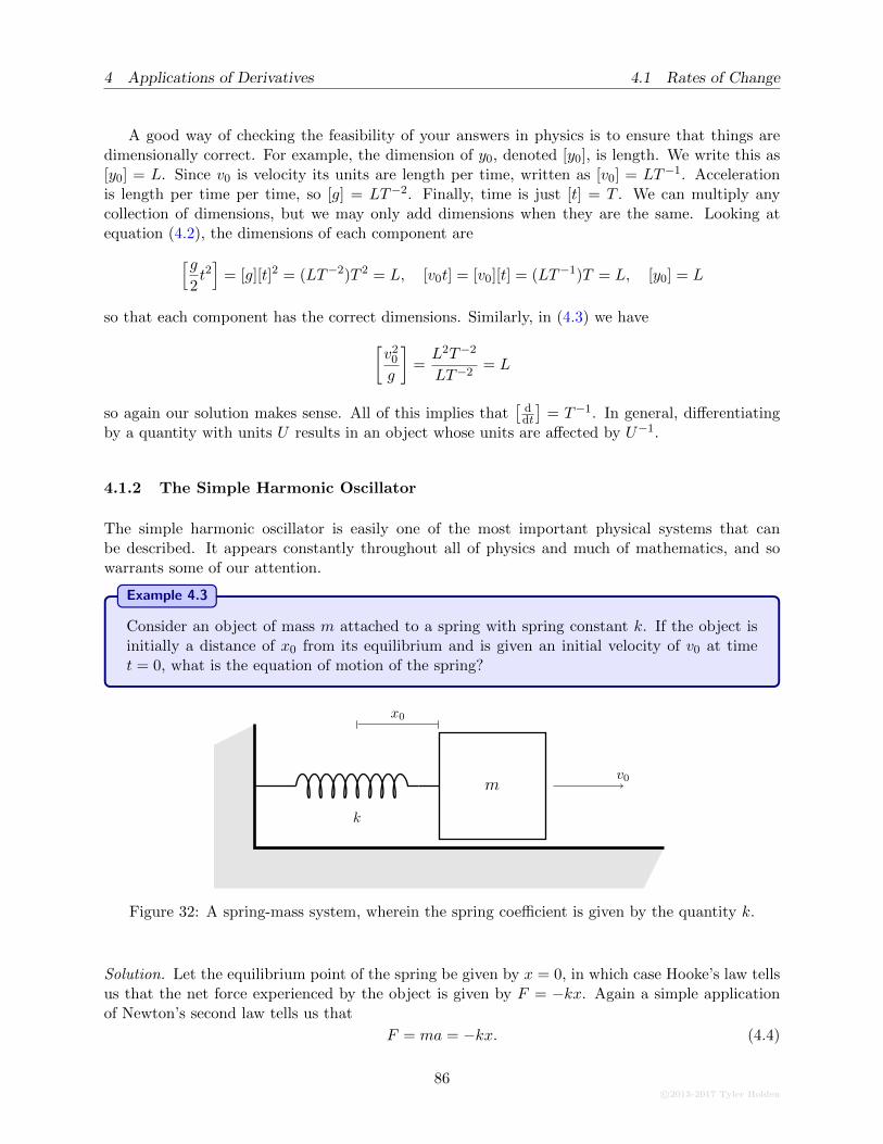
4 Applications of Derivatives 4.1 Rates of Change
A good way of checking the feasibility of your answers in physics is to ensure that things aredimensionally correct. For example, the dimension of y0, denoted [y0], is length. We write this as[y0] = L. Since v0 is velocity its units are length per time, written as [v0] = LT−1. Accelerationis length per time per time, so [g] = LT−2. Finally, time is just [t] = T . We can multiply anycollection of dimensions, but we may only add dimensions when they are the same. Looking atequation (4.2), the dimensions of each component are
[g2t2]
= [g][t]2 = (LT−2)T 2 = L, [v0t] = [v0][t] = (LT−1)T = L, [y0] = L
so that each component has the correct dimensions. Similarly, in (4.3) we have
[v2
0
g
]=L2T−2
LT−2= L
so again our solution makes sense. All of this implies that[
ddt
]= T−1. In general, differentiating
by a quantity with units U results in an object whose units are affected by U−1.
4.1.2 The Simple Harmonic Oscillator
The simple harmonic oscillator is easily one of the most important physical systems that canbe described. It appears constantly throughout all of physics and much of mathematics, and sowarrants some of our attention.
Example 4.3
Consider an object of mass m attached to a spring with spring constant k. If the object isinitially a distance of x0 from its equilibrium and is given an initial velocity of v0 at timet = 0, what is the equation of motion of the spring?
k
mv0
x0
Figure 32: A spring-mass system, wherein the spring coefficient is given by the quantity k.
Solution. Let the equilibrium point of the spring be given by x = 0, in which case Hooke’s law tellsus that the net force experienced by the object is given by F = −kx. Again a simple applicationof Newton’s second law tells us that
F = ma = −kx. (4.4)
86c©2013-2017 Tyler Holden
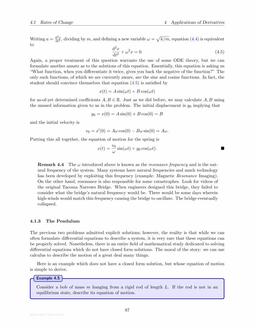
4.1 Rates of Change 4 Applications of Derivatives
Writing a = d2xdt2
, dividing by m, and defining a new variable ω =√k/m, equation (4.4) is equivalent
tod2x
dt2+ ω2x = 0. (4.5)
Again, a proper treatment of this question warrants the use of some ODE theory, but we canformulate another ansatz as to the solutions of this equation. Essentially, this equation is asking us“What function, when you differentiate it twice, gives you back the negative of the function?” Theonly such functions, of which we are currently aware, are the sine and cosine functions. In fact, thestudent should convince themselves that equation (4.5) is satisfied by
x(t) = A sin(ωt) +B cos(ωt)
for as-of-yet determined coefficients A,B ∈ R. Just as we did before, we may calculate A,B usingthe unused information given to us in the problem. The initial displacement is y0 implying that
y0 = x(0) = A sin(0) +B cos(0) = B
and the initial velocity is
v0 = x′(0) = Aω cos(0)−Bω sin(0) = Aω.
Putting this all together, the equation of motion for the spring is
x(t) =v0
ωsin(ωt) + y0 cos(ωt). �
Remark 4.4 The ω introduced above is known as the resonance frequency and is the nat-ural frequency of the system. Many systems have natural frequencies and much technologyhas been developed by exploiting this frequency (example: Magnetic Resonance Imaging).On the other hand, resonance is also responsible for some catastrophes. Look for videos ofthe original Tacoma Narrows Bridge. When engineers designed this bridge, they failed toconsider what the bridge’s natural frequency would be. There would be some days whereinhigh-winds would match this frequency causing the bridge to oscillate. The bridge eventuallycollapsed.
4.1.3 The Pendulum
The previous two problems admitted explicit solutions; however, the reality is that while we canoften formulate differential equations to describe a system, it is very rare that these equations canbe properly solved. Nonetheless, there is an entire field of mathematical study dedicated to solvingdifferential equations which do not have closed form solutions. The moral of the story: we can usecalculus to describe the motion of a great deal many things.
Here is an example which does not have a closed form solution, but whose equation of motionis simple to derive.
Example 4.5
Consider a bob of mass m hanging from a rigid rod of length L. If the rod is not in anequilibrium state, describe its equation of motion.
c©2013-2017 Tyler Holden
87
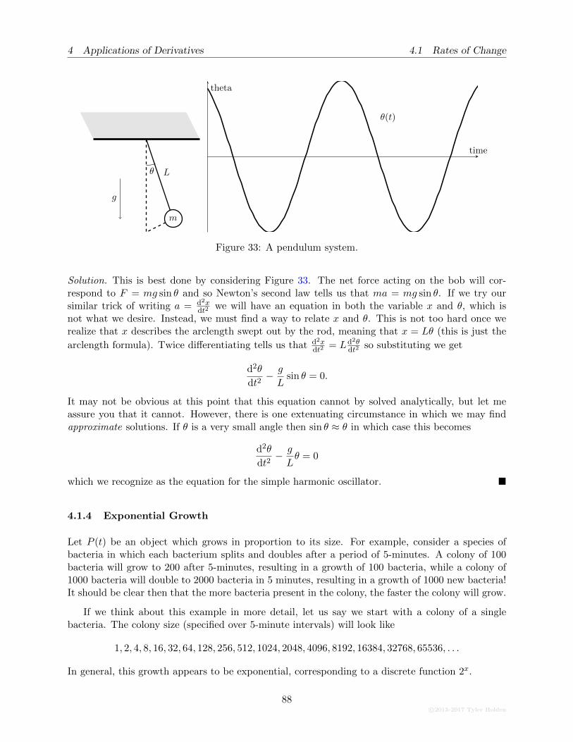
4 Applications of Derivatives 4.1 Rates of Change
m
L
g
θ
θ(t)
time
theta
Figure 33: A pendulum system.
Solution. This is best done by considering Figure 33. The net force acting on the bob will cor-respond to F = mg sin θ and so Newton’s second law tells us that ma = mg sin θ. If we try oursimilar trick of writing a = d2x
dt2we will have an equation in both the variable x and θ, which is
not what we desire. Instead, we must find a way to relate x and θ. This is not too hard once werealize that x describes the arclength swept out by the rod, meaning that x = Lθ (this is just the
arclength formula). Twice differentiating tells us that d2xdt2
= Ld2θdt2
so substituting we get
d2θ
dt2− g
Lsin θ = 0.
It may not be obvious at this point that this equation cannot by solved analytically, but let meassure you that it cannot. However, there is one extenuating circumstance in which we may findapproximate solutions. If θ is a very small angle then sin θ ≈ θ in which case this becomes
d2θ
dt2− g
Lθ = 0
which we recognize as the equation for the simple harmonic oscillator. �
4.1.4 Exponential Growth
Let P (t) be an object which grows in proportion to its size. For example, consider a species ofbacteria in which each bacterium splits and doubles after a period of 5-minutes. A colony of 100bacteria will grow to 200 after 5-minutes, resulting in a growth of 100 bacteria, while a colony of1000 bacteria will double to 2000 bacteria in 5 minutes, resulting in a growth of 1000 new bacteria!It should be clear then that the more bacteria present in the colony, the faster the colony will grow.
If we think about this example in more detail, let us say we start with a colony of a singlebacteria. The colony size (specified over 5-minute intervals) will look like
1, 2, 4, 8, 16, 32, 64, 128, 256, 512, 1024, 2048, 4096, 8192, 16384, 32768, 65536, . . .
In general, this growth appears to be exponential, corresponding to a discrete function 2x.
88c©2013-2017 Tyler Holden
4.1 Rates of Change 4 Applications of Derivatives
Modelling exponential growth is often simplified by assuming continuous rather than discretegrowth, and it turns out that this is actually one of the motivating example for defining Euler’snumber e. Perhaps the easiest way to see this is in the language of investment. Assume that youare given an initial investment I0 which grows with an interest rate r. If we compound the interestannually (once per year) then after one year we have I0(1 + r) dollars. If we compound the interestsemi-annually (twice per year) then we take half the interest rate r/2 and compound twice to get
I0
(1 +
r
2
)(1 +
r
2
)= I0
(1 +
r
2
)2.
Similarly, if we compounded the interest n times in a year, we would be left with the equationI0
(1 + r
n
)n. The idea of continuously compounding interest will then occur as we let n → ∞.
Namely, the amount of money earned after one year will be
I0 limn→∞
(1 +
r
n
)n.
Now what happens if we make the change of variable x = 1n so that as n→∞ we have x→ 0. Our
equation then becomes
I0 limn→∞
(1 +
r
n
)n= I0 lim
x→0(1 + rx)1/x = I0e
r;
that is, the number e represents the proportion by which your money will increase if compoundedcontinuously over the course of a year. If we had started with $1 then after one year of continuousinterest at 1% we would finish the year with $e. This is the sense to which e is natural, it representscontinuous growth.
Now if we return to our bacteria example, let us assume that our bacteria population growsat a continuous rate which is proportional to its population. That is, there is some constant ofproportionality k such that dP
dt = kP . What kind of function satisfies this differential equation?A bit of inspection actually reveals that if I0 is the initial population, P (t) = I0e
kt satisfies theequation, since
dP
dt=
d
dtI0e
kt = I0kekt = kP (t).
Hence any quantity which grows (or shrinks) continuously and proportional to its population sizeis modelled with an exponential function.
Example 4.6
If an original investment of $100 is invested at a rate of 6% and compounded continuously,how long will it take for the investment to triple in size?
Solution. Our model is given by I(t) = 100e0.06t and we would like to find the t such that I(t) = 300(since 300 is triple the number 100). Indeed, we may solve to find that 300 = 100e0.6t implies
3 = e0.06t ⇒ 0.06t = ln(3) ⇒ t =ln(3)
0.06≈ 18.3 years. �
c©2013-2017 Tyler Holden
89
4 Applications of Derivatives 4.1 Rates of Change
Example 4.7
Assume that a culture of bacteria has an initial population of 100 bacteria, which becomes350 bacteria after 10-hours. Determine the population of the bacteria after 2-days.
Solution. We know that our growth curve is modelled by the formula P (t) = 100ekt, for t measuredin hours. We are also told that
P (10) = 100e10k = 350,
which will allow us to solve for the growth rate k. Indeed,
100e10k = 350 ⇒ e10k = 3.5 ⇒ 10k = ln(3.5) ⇒ k =ln(3.5)
10.
To be consistent with our choice of units, we note that two days is 48-hours, so the population aftertwo days is
P (48) = 100e48k = 100e48ln(3.5)
10 = 100eln(3.54.8) = 100 · 3.54.8 ≈ 40881 bacteria. �
Example 4.8
Caffeine in the blood stream has a biological half-life of 5-hours. If I drink a venti cafeAmericano from Starbucks, consisting of 300mg of caffeine, at 8am in the morning. Howmuch caffeine will be in my system by midnight?
Solution. Let us that t = 0 corresponds to 8am, so that midnight is t = 16. The amount of caffeineis modelled by the equation c(t) = 300ekt and we know that c(5) = 300e5k = 150 (since 150 is half
of 300). We may solve for k to find that k = − ln(2)30 . Hence at time t = 16 we have
c(16) = 300e−16ln(2)5 = 300 · 2−16/5 ≈ 32.64 mg. �
One can show that if the half life of a substance is a time t0, then the growth/decay rate k is
always given by k = − ln(2)t0
.
Logistic Growth: While this model of exponential growth can be quite useful for modellingshort term growth, it quickly becomes unrealistic. Exponential functions grow incredibly quickly:in fact, if a species of bacteria grow at the same rate as in Example 4.7, then a single bacteriumwould grow into a colony with the same mass as the entire Earth in about one month!
Our exponential model breaks down in the long term as it fails to incorporate things likecompetition with other bacteria, or the limited number of resources available to the bacteria. If weknow a priori that the bacteria only have enough resources to sustain a certain size colony, we canadapt our model to take that into consideration. The maximum number M of the species is calledthe carrying capacity, and changes our model to be
dP
dt= kP
(1− P
M
). (4.6)
90c©2013-2017 Tyler Holden
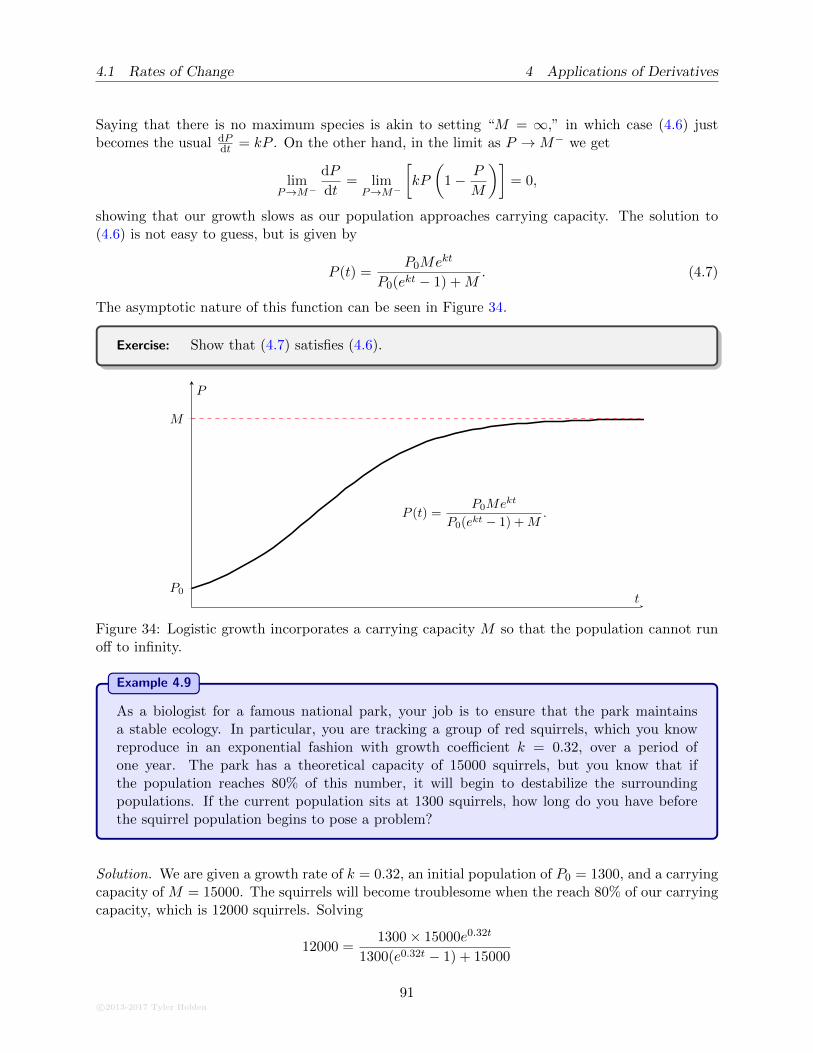
4.1 Rates of Change 4 Applications of Derivatives
Saying that there is no maximum species is akin to setting “M = ∞,” in which case (4.6) justbecomes the usual dP
dt = kP . On the other hand, in the limit as P →M− we get
limP→M−
dP
dt= lim
P→M−
[kP
(1− P
M
)]= 0,
showing that our growth slows as our population approaches carrying capacity. The solution to(4.6) is not easy to guess, but is given by
P (t) =P0Mekt
P0(ekt − 1) +M. (4.7)
The asymptotic nature of this function can be seen in Figure 34.
Exercise: Show that (4.7) satisfies (4.6).
P0
M
P (t) =P0Mekt
P0(ekt − 1) +M.
t
P
Figure 34: Logistic growth incorporates a carrying capacity M so that the population cannot runoff to infinity.
Example 4.9
As a biologist for a famous national park, your job is to ensure that the park maintainsa stable ecology. In particular, you are tracking a group of red squirrels, which you knowreproduce in an exponential fashion with growth coefficient k = 0.32, over a period ofone year. The park has a theoretical capacity of 15000 squirrels, but you know that ifthe population reaches 80% of this number, it will begin to destabilize the surroundingpopulations. If the current population sits at 1300 squirrels, how long do you have beforethe squirrel population begins to pose a problem?
Solution. We are given a growth rate of k = 0.32, an initial population of P0 = 1300, and a carryingcapacity of M = 15000. The squirrels will become troublesome when the reach 80% of our carryingcapacity, which is 12000 squirrels. Solving
12000 =1300× 15000e0.32t
1300(e0.32t − 1) + 15000
c©2013-2017 Tyler Holden
91
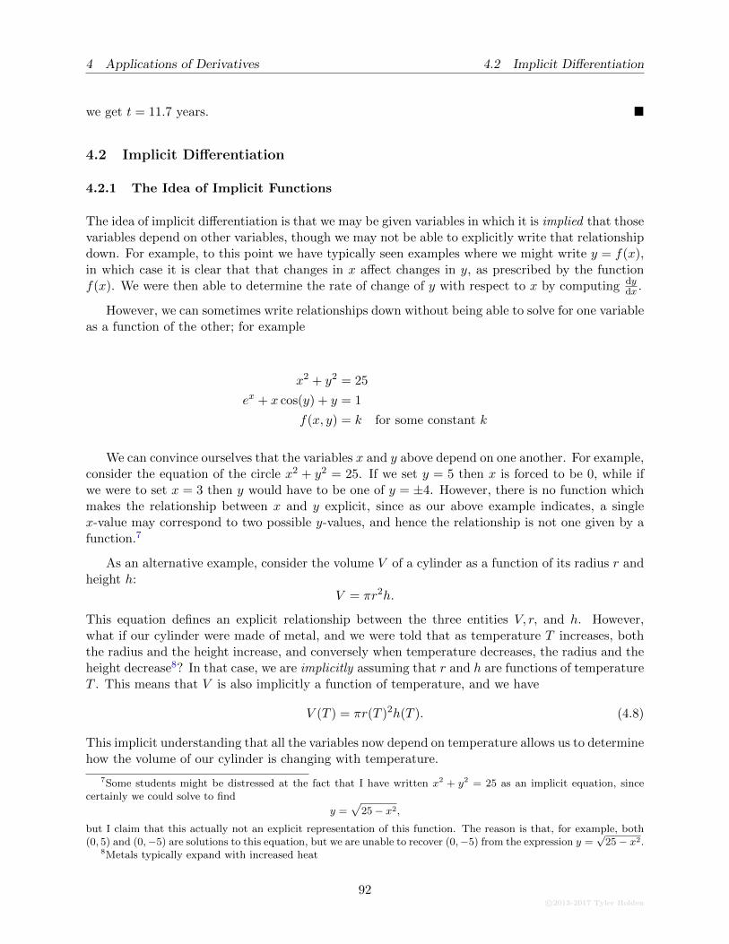
4 Applications of Derivatives 4.2 Implicit Differentiation
we get t = 11.7 years. �
4.2 Implicit Differentiation
4.2.1 The Idea of Implicit Functions
The idea of implicit differentiation is that we may be given variables in which it is implied that thosevariables depend on other variables, though we may not be able to explicitly write that relationshipdown. For example, to this point we have typically seen examples where we might write y = f(x),in which case it is clear that that changes in x affect changes in y, as prescribed by the functionf(x). We were then able to determine the rate of change of y with respect to x by computing dy
dx .
However, we can sometimes write relationships down without being able to solve for one variableas a function of the other; for example
x2 + y2 = 25
ex + x cos(y) + y = 1
f(x, y) = k for some constant k
We can convince ourselves that the variables x and y above depend on one another. For example,consider the equation of the circle x2 + y2 = 25. If we set y = 5 then x is forced to be 0, while ifwe were to set x = 3 then y would have to be one of y = ±4. However, there is no function whichmakes the relationship between x and y explicit, since as our above example indicates, a singlex-value may correspond to two possible y-values, and hence the relationship is not one given by afunction.7
As an alternative example, consider the volume V of a cylinder as a function of its radius r andheight h:
V = πr2h.
This equation defines an explicit relationship between the three entities V, r, and h. However,what if our cylinder were made of metal, and we were told that as temperature T increases, boththe radius and the height increase, and conversely when temperature decreases, the radius and theheight decrease8? In that case, we are implicitly assuming that r and h are functions of temperatureT . This means that V is also implicitly a function of temperature, and we have
V (T ) = πr(T )2h(T ). (4.8)
This implicit understanding that all the variables now depend on temperature allows us to determinehow the volume of our cylinder is changing with temperature.
7Some students might be distressed at the fact that I have written x2 + y2 = 25 as an implicit equation, sincecertainly we could solve to find
y =√
25− x2,but I claim that this actually not an explicit representation of this function. The reason is that, for example, both(0, 5) and (0,−5) are solutions to this equation, but we are unable to recover (0,−5) from the expression y =
√25− x2.
8Metals typically expand with increased heat
92c©2013-2017 Tyler Holden
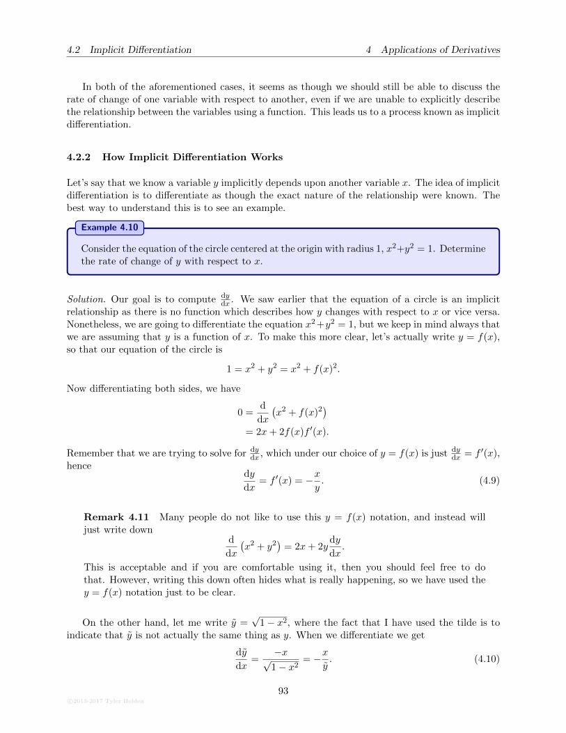
4.2 Implicit Differentiation 4 Applications of Derivatives
In both of the aforementioned cases, it seems as though we should still be able to discuss therate of change of one variable with respect to another, even if we are unable to explicitly describethe relationship between the variables using a function. This leads us to a process known as implicitdifferentiation.
4.2.2 How Implicit Differentiation Works
Let’s say that we know a variable y implicitly depends upon another variable x. The idea of implicitdifferentiation is to differentiate as though the exact nature of the relationship were known. Thebest way to understand this is to see an example.
Example 4.10
Consider the equation of the circle centered at the origin with radius 1, x2+y2 = 1. Determinethe rate of change of y with respect to x.
Solution. Our goal is to compute dydx . We saw earlier that the equation of a circle is an implicit
relationship as there is no function which describes how y changes with respect to x or vice versa.Nonetheless, we are going to differentiate the equation x2 +y2 = 1, but we keep in mind always thatwe are assuming that y is a function of x. To make this more clear, let’s actually write y = f(x),so that our equation of the circle is
1 = x2 + y2 = x2 + f(x)2.
Now differentiating both sides, we have
0 =d
dx
(x2 + f(x)2
)
= 2x+ 2f(x)f ′(x).
Remember that we are trying to solve for dydx , which under our choice of y = f(x) is just dy
dx = f ′(x),hence
dy
dx= f ′(x) = −x
y. (4.9)
Remark 4.11 Many people do not like to use this y = f(x) notation, and instead willjust write down
d
dx
(x2 + y2
)= 2x+ 2y
dy
dx.
This is acceptable and if you are comfortable using it, then you should feel free to dothat. However, writing this down often hides what is really happening, so we have used they = f(x) notation just to be clear.
On the other hand, let me write y =√
1− x2, where the fact that I have used the tilde is toindicate that y is not actually the same thing as y. When we differentiate we get
dy
dx=
−x√1− x2
= −xy. (4.10)
c©2013-2017 Tyler Holden
93
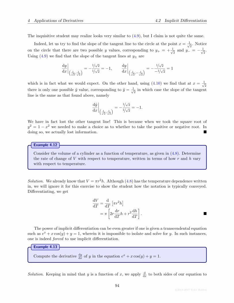
4 Applications of Derivatives 4.2 Implicit Differentiation
The inquisitive student may realize looks very similar to (4.9), but I claim is not quite the same.
Indeed, let us try to find the slope of the tangent line to the circle at the point x = 1√2. Notice
on the circle that there are two possible y values, corresponding to y+ = + 1√2
and y− = − 1√2.
Using (4.9) we find that the slope of the tangent lines at y± are
dy
dx
∣∣∣∣(1√2, 1√
2
) = −1/√
2
1/√
2= −1,
dy
dx
∣∣∣∣(1√2,− 1√
2
) = −1/√
2
−1/√
2= 1
which is in fact what we would expect. On the other hand, using (4.10) we find that at x = 1√2
there is only one possible y value, corresponding to y = 1√2
in which case the slope of the tangent
line is the same as that found above, namely
dy
dx
∣∣∣∣(1√2, 1√
2
) = −1/√
2
1/√
2= −1.
We have in fact lost the other tangent line! This is because when we took the square root ofy2 = 1 − x2 we needed to make a choice as to whether to take the positive or negative root. Indoing so, we actually lost information. �
Example 4.12
Consider the volume of a cylinder as a function of temperature, as given in (4.8). Determinethe rate of change of V with respect to temperature, written in terms of how r and h varywith respect to temperature.
Solution. We already know that V = πr2h. Although (4.8) has the temperature dependence writtenin, we will ignore it for this exercise to show the student how the notation is typically conveyed.Differentiating, we get
dV
dT=
d
dT
[πr2h
]
= π
[2r
dr
dTh+ r2 dh
dT
]. �
The power of implicit differentiation can be even greater if one is given a transcendental equationsuch as ex + x cos(y) + y = 1, wherein it is impossible to isolate and solve for y. In such instances,one is indeed forced to use implicit differentiation.
Example 4.13
Compute the derivative dydx of y in the equation ex + x cos(y) + y = 1.
Solution. Keeping in mind that y is a function of x, we apply ddx to both sides of our equation to
94c©2013-2017 Tyler Holden
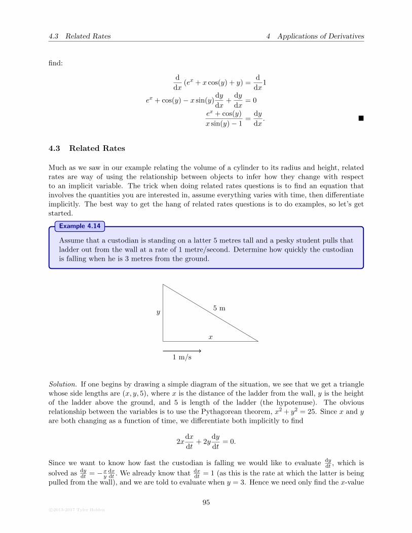
4.3 Related Rates 4 Applications of Derivatives
find:
d
dx(ex + x cos(y) + y) =
d
dx1
ex + cos(y)− x sin(y)dy
dx+
dy
dx= 0
ex + cos(y)
x sin(y)− 1=
dy
dx. �
4.3 Related Rates
Much as we saw in our example relating the volume of a cylinder to its radius and height, relatedrates are way of using the relationship between objects to infer how they change with respectto an implicit variable. The trick when doing related rates questions is to find an equation thatinvolves the quantities you are interested in, assume everything varies with time, then differentiateimplicitly. The best way to get the hang of related rates questions is to do examples, so let’s getstarted.
Example 4.14
Assume that a custodian is standing on a latter 5 metres tall and a pesky student pulls thatladder out from the wall at a rate of 1 metre/second. Determine how quickly the custodianis falling when he is 3 metres from the ground.
x
5 my
1 m/s
Solution. If one begins by drawing a simple diagram of the situation, we see that we get a trianglewhose side lengths are (x, y, 5), where x is the distance of the ladder from the wall, y is the heightof the ladder above the ground, and 5 is length of the ladder (the hypotenuse). The obviousrelationship between the variables is to use the Pythagorean theorem, x2 + y2 = 25. Since x and yare both changing as a function of time, we differentiate both implicitly to find
2xdx
dt+ 2y
dy
dt= 0.
Since we want to know how fast the custodian is falling we would like to evaluate dydt , which is
solved as dydt = −x
ydxdt . We already know that dx
dt = 1 (as this is the rate at which the latter is beingpulled from the wall), and we are told to evaluate when y = 3. Hence we need only find the x-value
c©2013-2017 Tyler Holden
95
4 Applications of Derivatives 4.3 Related Rates
which corresponds to a y-value of 3. The Pythagorean theorem again implies that if y = 3 thenx =√
52 − 32 = 4, so thatdy
dt= −4
3(1) = −4
3.
Thus the custodian is falling at 4/3 metres per second. �
Example 4.15
A sphere is shrinking in such a way that its surface area changes at a constant rate of 1 unit2
per time. Find the rate at which the diameter of the sphere is decreasing when the diameteris 5 units.
Solution. First, we look at the quantities involved. We are given information about the surfacearea A of the sphere, and its diameter δ. We know that the formula for the surface area of a sphereis given by A = 4πr2 where r is the radius of the sphere. This is not quite what we want though,since we are interested in the diameter. Luckily, we also know that the radius is half the diameter,so that r = δ/2. Substituting this we find that
A = 4π
(δ
2
)2
= πδ2.
Both the area and the diameter are changing with time, so when we differentiate we will have todo so implicitly with respect to time:
dA
dt= 2πδ
dδ
dt.
We want to know dδdt as this represents the change in the diameter with respect to time, so we solve
to find thatdδ
dt=
1
2πδ
dA
dt.
Since A is decreasing at a rate of 1 unit2 per time, we set dAdt = −1, where the negative sign
indicates that the quantity is decreasing. Thus we know every quantity on the right hand side, sowe may substitute to find that
dδ
dt=
1
2π · 5(−1) = − 1
10π. �
Example 4.16
Consider a square pyramid which is being filled with water. The base square has length andwidth both equal to L > 0 and the height of the apex of the pyramid is also a distance L fromthe base. As a function of the current height of the liquid, how must we poor the mysteriousquantity into the pyramid such that the rate of change of the height of the material does notdepend on the size of the base square. Is this rate dependent on the height of the pyramid?
Solution. Let V be the volume of the liquid contained in the pyramid, which we know is an increas-ing function in time. We have the capability of adjusting the flow rate, which corresponds to the
96c©2013-2017 Tyler Holden
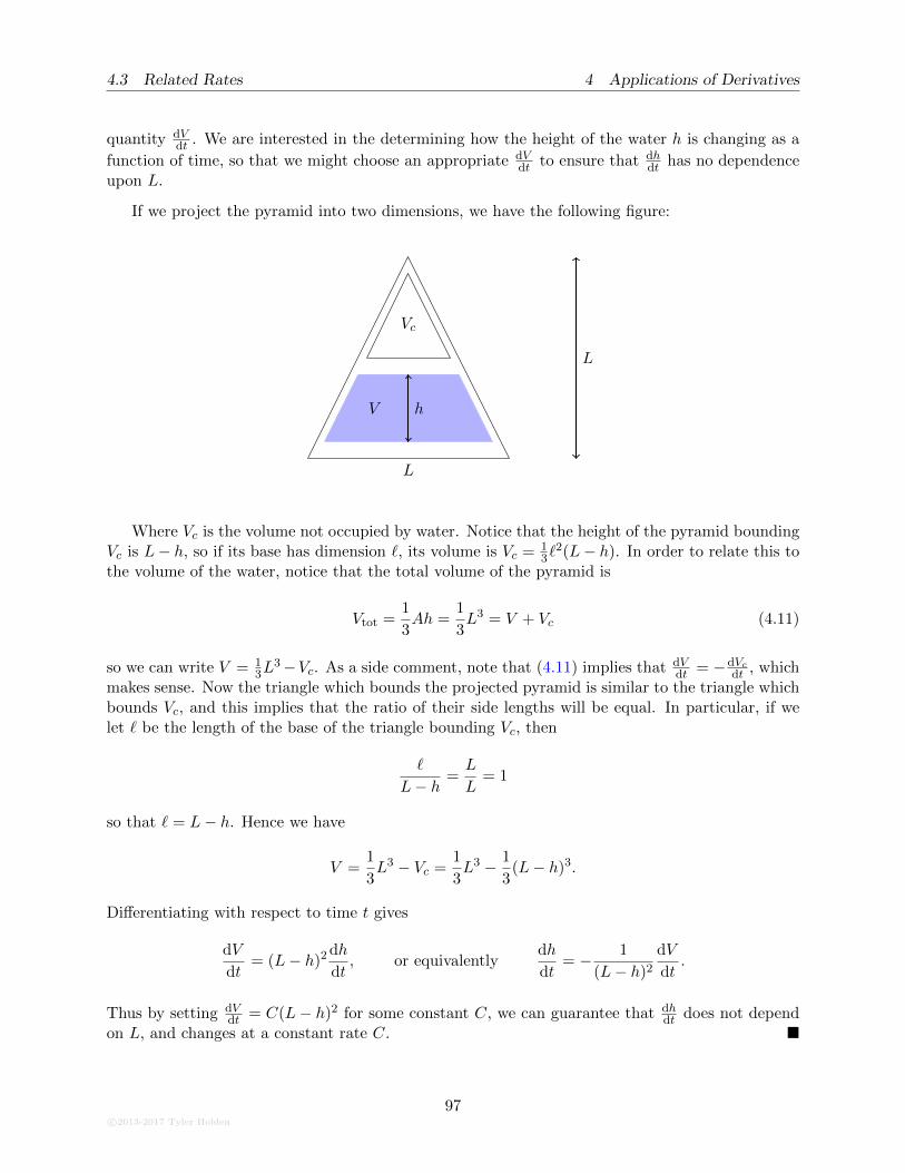
4.3 Related Rates 4 Applications of Derivatives
quantity dVdt . We are interested in the determining how the height of the water h is changing as a
function of time, so that we might choose an appropriate dVdt to ensure that dh
dt has no dependenceupon L.
If we project the pyramid into two dimensions, we have the following figure:
L
hV
L
Vc
Where Vc is the volume not occupied by water. Notice that the height of the pyramid boundingVc is L− h, so if its base has dimension `, its volume is Vc = 1
3`2(L− h). In order to relate this to
the volume of the water, notice that the total volume of the pyramid is
Vtot =1
3Ah =
1
3L3 = V + Vc (4.11)
so we can write V = 13L
3−Vc. As a side comment, note that (4.11) implies that dVdt = −dVc
dt , whichmakes sense. Now the triangle which bounds the projected pyramid is similar to the triangle whichbounds Vc, and this implies that the ratio of their side lengths will be equal. In particular, if welet ` be the length of the base of the triangle bounding Vc, then
`
L− h =L
L= 1
so that ` = L− h. Hence we have
V =1
3L3 − Vc =
1
3L3 − 1
3(L− h)3.
Differentiating with respect to time t gives
dV
dt= (L− h)2 dh
dt, or equivalently
dh
dt= − 1
(L− h)2
dV
dt.
Thus by setting dVdt = C(L− h)2 for some constant C, we can guarantee that dh
dt does not dependon L, and changes at a constant rate C. �
c©2013-2017 Tyler Holden
97
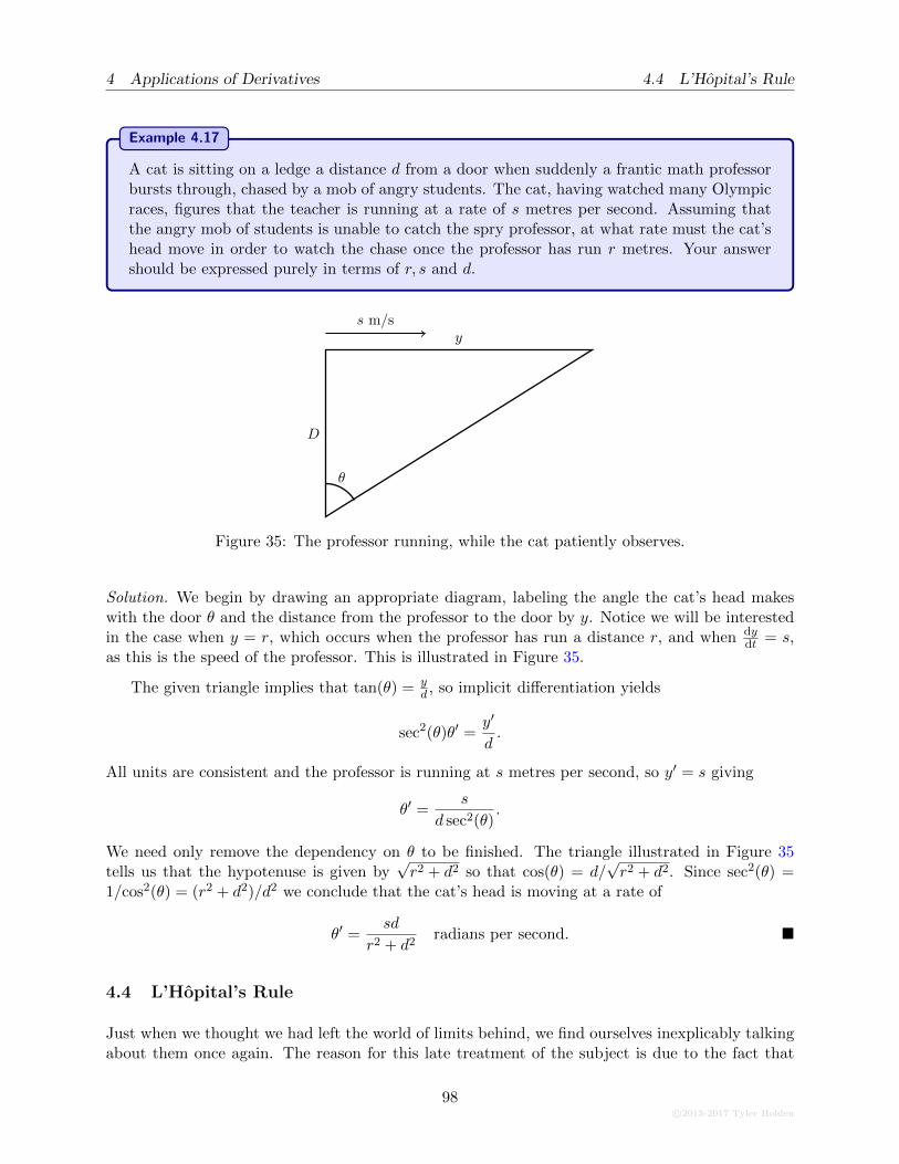
4 Applications of Derivatives 4.4 L’Hopital’s Rule
Example 4.17
A cat is sitting on a ledge a distance d from a door when suddenly a frantic math professorbursts through, chased by a mob of angry students. The cat, having watched many Olympicraces, figures that the teacher is running at a rate of s metres per second. Assuming thatthe angry mob of students is unable to catch the spry professor, at what rate must the cat’shead move in order to watch the chase once the professor has run r metres. Your answershould be expressed purely in terms of r, s and d.
D
y
θ
s m/s
Figure 35: The professor running, while the cat patiently observes.
Solution. We begin by drawing an appropriate diagram, labeling the angle the cat’s head makeswith the door θ and the distance from the professor to the door by y. Notice we will be interestedin the case when y = r, which occurs when the professor has run a distance r, and when dy
dt = s,as this is the speed of the professor. This is illustrated in Figure 35.
The given triangle implies that tan(θ) = yd , so implicit differentiation yields
sec2(θ)θ′ =y′
d.
All units are consistent and the professor is running at s metres per second, so y′ = s giving
θ′ =s
d sec2(θ).
We need only remove the dependency on θ to be finished. The triangle illustrated in Figure 35tells us that the hypotenuse is given by
√r2 + d2 so that cos(θ) = d/
√r2 + d2. Since sec2(θ) =
1/cos2(θ) = (r2 + d2)/d2 we conclude that the cat’s head is moving at a rate of
θ′ =sd
r2 + d2radians per second. �
4.4 L’Hopital’s Rule
Just when we thought we had left the world of limits behind, we find ourselves inexplicably talkingabout them once again. The reason for this late treatment of the subject is due to the fact that
98c©2013-2017 Tyler Holden
4.4 L’Hopital’s Rule 4 Applications of Derivatives
we had initially sheltered the student from the cruel world of limits, choosing to show you only thenicest limits which could be computed via some algebraic magic. Now, with a much more developedtoolbox, we venture into the treatment of these remaining limits.
4.4.1 Standard Indeterminate Type
We have seen that in the case of many functions formed from quotients, if both the numeratorand denominator independently gave finite limits and the denominator was not zero, then we couldsimply apply the limit law for quotients. Similarly, if only one of the numerator or denominatorgave a limit of 0 then one could often convince him/herself that the limit was either 0 or infinity,respectively. The troublesome point comes when both the numerator and the denominator bothapproach zero. How then can we treat such problems in general? We begin with a classification ofthe types of problems which can occur:
Definition 4.18
Let f(x) and g(x) be two functions,
1. If limx→c
f(x) = limx→c
g(x) = 0 then we say that limx→c
f(x)
g(x)is indeterminate of type 0/0.
2. If limx→c|f(x)| = lim
x→c|g(x)| = ∞ then we say that lim
x→c
f(x)
g(x)is indeterminate of type
∞/∞.
Note: If we take the limit as x → ∞ or x → −∞, or either of the one sided limits x → c±
we will still say that the limits are of the above indeterminate types.
Indeterminate forms are precisely the aforementioned pesky functions. Here is how we attackthem.
Theorem 4.19: L’Hopital’s Rule
Suppose that f(x) and g(x) are differentiable in an interval containing c, and that the limit
limx→c
f(x)
g(x)is indeterminate of either type 0/0 or type∞/∞. If one of the following conditions
holds:
1. The limit limx→c
f ′(x)
g′(x)exists,
2. There is an interval containing c on which g′ is never zero,
3. There is an interval containing c in which g′ does not switch signs infinitely often,
then limx→c
f(x)
g(x)exists and lim
x→c
f(x)
g(x)= lim
x→c
f ′(x)
g′(x).
c©2013-2017 Tyler Holden
99
4 Applications of Derivatives 4.4 L’Hopital’s Rule
Example 4.20
Compute the limit limx→0
e2x − 1
sin(x).
Solution. A quick check shows that this limit is of indeterminate type 0/0, since as x→ 0 we haveboth e2 − 1→ 0 and sin(x)→ 0. Hence we may apply L’Hopital’s rule to find that
limx→0
e2x − 1
sin(x)= lim
x→0
ddx
[e2x − 1
]
ddx sin(x)
= limx→0
2e2x
cos(x)= 2. �
Remark 4.21
1. Note that we take the derivative of both the top and the bottom separately. Many stu-dents accidentally take the derivative of the quantity f(x)/g(x), which by the quotientrule is very different than f ′(x)/g′(x).
2. It is absolutely essential that the student first check that the limit is of indeterminatetype. L’Hopital’s Rule does not hold if the limit is not of indeterminatetype. Indeed, we recall that
limx→0
sin(x)
cos(x)=
0
1= 0,
so this limit is not of indeterminate type and can be evaluated quite simply. On theother hand, if we had tried to apply L’Hopital’s Rule we would have gotten
limx→0
sin(x)
cos(x)= lim
x→0
cos(x)
− sin(x)= −∞
which is clearly not equal to 0. We thus re-emphasize that the student MUST checkthat the limit is indeterminate.
There may be instances in which a single application of L’Hopital’s Rule is not sufficient and thestudent will be required to apply the rule multiple times, as the following example demonstrates.
Example 4.22
Compute the limit limx→∞
ex2
x4.
Solution. It is easy to convince ourselves that this is indeterminate of type ∞/∞, so that we may
100c©2013-2017 Tyler Holden
4.4 L’Hopital’s Rule 4 Applications of Derivatives
apply L’Hopital’s Rule. Indeed, we find that
limx→∞
ex2
x4= lim
x→∞
2xex2
4x3
=1
2limx→∞
ex2
x2again type ∞/∞
=1
2limx→∞
2xex2
2x
=1
2limx→∞
ex2
=∞. �
In the previous example, we were required to apply L’Hopital’s Rule twice. It is also importantto note that the solution does not have to be finite: We can still have L’Hopital give us infinitesolutions.
Exercise: We say that a function f(x) “grows” faster than g(x) if
limx→0
g(x)
f(x)= 0, or equivalently lim
x→0
f(x)
g(x)=∞.
Using L’Hopital’s Rule, show that ex grows faster than any polynomial; that is, show thatex is faster than xn for any n.
Example 4.23
Compute the limit limx→0
ex − 1− xx2
.
Solution. This is again indeterminate of type 0/0, so we use L’Hopital and compute
limx→0
ex − 1− xx2
= limx→0
ex − 1
2xindeterminate of type 0/0
= limx→0
ex
2=
1
2. �
Example 4.24
Determine the limit limx→0
xenx − x1− cos(nx)
for n 6= 0.
Solution. It is easy to check that this is of type 0/0, so we can apply L’Hopital to get
limx→0
xenx − x1− cos(nx)
〈H〉= lim
x→0
enx + nxenx − 1
n sin(nx)
〈H〉= lim
x→0
nenx + nenx + n2xenx
n2 cos(nx)
=2n
n2=
2
n. �
c©2013-2017 Tyler Holden
101
4 Applications of Derivatives 4.4 L’Hopital’s Rule
Example 4.25
If f(x) is twice differentiable at c and f ′′(x) is continuous at c, compute the limits
limh→0
f(c+ h)− f(c− h)
2h, lim
h→0
f(c+ h)− 2f(c) + f(c− h)
h2. (4.12)
Solution. We recognize that the limit in question is indeterminate of type 0/0 and so we have
limh→0
f(c+ h)− f(c− h)
2h
〈H〉= lim
h→0
f ′(c+ h)− (−1)f ′(c− h)
2= f ′(c) (4.13)
wherein again we stress that we must differentiate with respect to h.
The second limit in (4.12) is a little bit harder to see without using L’Hopital, so let’s just goahead and compute to find
limh→0
f(c+ h)− 2f(c) + f(c− h)
h2
〈H〉= lim
h→0
f ′(c+ h)− f ′(c− h)
2h
by L’Hopitalwith type 0/0
= (f ′)′(c) by (4.13)
= f ′′(c). �
4.4.2 Other Indeterminate Types
Having formulated a strategy for computing limits of indeterminate quotients, we can adapt thestrategy above to other types of indeterminate forms. In particular, the remaining indeterminateforms are of type 0×∞,∞−∞, 1∞, 00 and ∞0. The strategy for dealing with each of these casesis to turn it into an indeterminate of type 0/0 or ∞/∞, as follows:
1. 0×∞: Possibly the easiest case to deal with, assume that we are given a limit of the form
limx→a
f(x)g(x), where limx→a
f(x) = 0, and limx→a
g(x) =∞.
We can thus turn this into 0/0 or ∞/∞ as
limx→a
f(x)
1/g(x)type 0/0, lim
x→a
g(x)
1/f(x)type ∞/∞.
2. ∞−∞: In contrast to the previous cases, these are possibly the hardest to transform intoone of 0/0 or ∞/∞. This case arises when we have a limit of the form:
limx→a
[f(x)− g(x)], where limx→a
f(x) =∞, and limx→a
g(x) =∞.
There is no algorithmic way to do this, so the student is required to use their math-skills tomanipulate such a limit into the desired form. Indeed, the student already has some practicewith these types of limits, such as limx→a
√x2 + 1− x.
102c©2013-2017 Tyler Holden
4.4 L’Hopital’s Rule 4 Applications of Derivatives
3. 1∞, 00,∞0: These cases are all handled identically, so we shall treat them together. For thesake of concreteness, assume we are given a limit of the form
limx→a
f(x)g(x), where limx→a
f(x) =∞, and limx→a
g(x) = 0
This case is handled by calling upon our old friend, implicit differentiation. Let y = f(x)g(x)
so that ln(y) = g(x) ln f(x). As we have seen previously, continuity of ex means that it issufficient to compute
limx→a
ln y, since limx→a
y = limx→a
eln(y) = elimx→a
ln y.
Now in the limit, ln(y) = g(x) ln f(x) is of type 0×∞, so we resort to case (1) which tells usthat we compute this limit by either
limx→a
g(x)
1/ ln f(x), or lim
x→a
ln f(x)
1/g(x).
In the case where f(x)→ 1 and g(x)→∞, or f(x)→ 0 and g(x)→ 0 we also get 0×∞ andso these cases are treated the same as above.
Note that there is no type 0∞ despite the fact that this seems like it could potentially beindeterminate. The intuitive reason for this is that as soon as the base becomes less than thenumber 1, taking powers will actually drive the limit closer to 0. Hence 0∞ = 0 and is not anindeterminate form.
Example 4.26
Compute the limit limx→0+
x ln(x).
Solution. In the limit as x → 0 the function ln(x) → −∞, so this limit is indeterminate of type0 × ∞. We now have to make a choice as to which component to invert. Let us choose to firstinvert the x, giving
limx→0+
x ln(x) = limx→0
ln(x)
1/x
〈H〉= lim
x→0
1/x
−1/x2
= limx→0−x = 0. �
Example 4.27
Determine the limit limx→0
[csc(x)− cot(x)]
Solution. It is easy to see that this limit is indeterminate of type ∞ −∞, but as everything istrigonometric, there is likely some simplification that can be performed. Writing everything in
c©2013-2017 Tyler Holden
103
4 Applications of Derivatives 4.5 Derivatives and the Shape of a Graph
terms of sin(x) and cos(x) we get
limx→0
[csc(x)− cot(x)] = limx→0
[1
sin(x)− cos(x)
sin(x)
]= lim
x→0
1− cos(x)
sin(x)
〈H〉= lim
x→0
sin(x)
cos(x)= 0.
Note that alternatively in this last step, we could have avoided using L’Hopital’s Rule by writing
limx→0
1− cos(x)
sin(x)= lim
x→0
1−cos(x)xx
sin(x)
=0
1= 0. �
Example 4.28
Determine the limit limx→∞
(1 +
a
x
)x.
Solution. It is not too hard to see that this is indeterminate of type 1∞, so we must take logarithmsin order to simplify our lives. Indeed, set y =
(1 + a
x
)xso that ln y = x ln
(1 + a
x
). In the limit as
x→∞, this is of type 0×∞, so we take the reciprocal of one of the elements and get
limx→∞
x ln(
1 +a
x
)= lim
x→∞
ln(1 + a
x
)
1/x
〈H〉= lim
x→∞
(−a/x2)/(1 + a
x
)
−1/x2
= limx→∞
a
1 + ax
= a.
Hence re-exponentiating, we get
limx→∞
(1 +
a
x
)x= e
limx→a
ln y= ea. �
4.5 Derivatives and the Shape of a Graph
4.6 First Derivative Information
Knowing something about the derivative of a function can often lead us to insights about what it’sgraph looks like.
Theorem 4.29
Let f(x) be a function with domain (a, b). If f ′(x) = 0 for all a < x < b then f(x) is aconstant function.
This is a very useful theorem, as it effectively tells us that the process of reversing differentiationresults in unique functions up to ad additive constant (Section 5.3). We can also use it to help usprove identities:
104c©2013-2017 Tyler Holden
4.6 First Derivative Information 4 Applications of Derivatives
Example 4.30
Show that for all x ≥ 0,2 arcsin(x) = arccos(1− 2x2).
Solution. Consider the function f(x) = 2 arcsin(x)− arccos(1− 2x2). Differentiating this functiongives
f ′(x) =2√
1− x2− 4x√
1− (1− 2x2)2.
By expanding the 1− (1− 2x2)2 term we get
1− (1− 2x2)2 = 1− (1− 4x2 + 4x4) = 4x2 − 4x4 = 4x2(1− x2)
and our above equation becomes
f ′(x) =2√
1− x2− 4x
2x√
1− x2=
2√1− x2
− 2√1− x2
= 0
Hence f(x) is a constant function, say f(x) = C. We need only determine the value of C, whichcan be done by substituting any value of x into our function. For example, substituting x = 0 gives
C = f(0) = 2 arcsin(0)− arccos(1) = 0− 0 = 0
so that C = 0. Thus f(x) = 0 for all x ≥ 0, and by re-arranging this we get the desired equality. �
Definition 4.31
We say that a function f(x) is increasing if whenever a < b then f(a) ≤ f(b), and strictlyincreasing if whenever a < b then f(a) < f(b).In the same vein, we say that f(x) is decreasing if whenever a < b then f(a) ≥ f(b), andstrictly decreasing if whenever a < b then f(a) > f(b).
Theorem 4.32
If f(x) is a function with domain (a, b) and f ′(x) > 0 for all a < x < b then f is strictlyincreasing.
The above theorem can also be used to determine where a function f(x) is increasing anddecreasing, by determining the intervals on which f ′(x) > 0 and f ′(x) < 0 respectively.
Example 4.33
Show that the function f(x) = arctan(x) is everywhere strictly increasing.
Solution. Differentiating f(x) we get
f ′(x) =1
1 + x2
which is positive for every real number x. Hence by Theorem 4.32 we know that f(x) = arctan(x)is everywhere strictly increasing. �
c©2013-2017 Tyler Holden
105
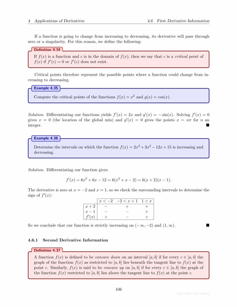
4 Applications of Derivatives 4.6 First Derivative Information
If a function is going to change from increasing to decreasing, its derivative will pass throughzero or a singularity. For this reason, we define the following:
Definition 4.34
If f(x) is a function and c is in the domain of f(x), then we say that c is a critical point off(x) if f ′(c) = 0 or f ′(c) does not exist.
Critical points therefore represent the possible points where a function could change from in-creasing to decreasing.
Example 4.35
Compute the critical points of the functions f(x) = x2 and g(x) = cos(x).
Solution. Differentiating our functions yields f ′(x) = 2x and g′(x) = − sin(x). Solving f ′(x) = 0gives x = 0 (the location of the global min) and g′(x) = 0 gives the points x = nπ for n aninteger. �
Example 4.36
Determine the intervals on which the function f(x) = 2x3 + 3x2− 12x+ 15 is increasing anddecreasing.
Solution. Differentiating our function gives
f ′(x) = 6x2 + 6x− 12 = 6(x2 + x− 2) = 6(x+ 2)(x− 1).
The derivative is zero at x = −2 and x = 1, so we check the surrounding intervals to determine thesign of f ′(x):
x < −2 −2 < x < 1 1 < x
x+ 2 − + +x− 1 − − +f ′(x) + − +
So we conclude that our function is strictly increasing on (−∞,−2) and (1,∞). �
4.6.1 Second Derivative Information
Definition 4.37
A function f(x) is defined to be concave down on an interval [a, b] if for every c ∈ [a, b] thegraph of the function f(x) as restricted to [a, b] lies beneath the tangent line to f(x) at thepoint c. Similarly, f(x) is said to be concave up on [a, b] if for every c ∈ [a, b] the graph ofthe function f(x) restricted to [a, b] lies above the tangent line to f(x) at the point c.
106c©2013-2017 Tyler Holden
4.6 First Derivative Information 4 Applications of Derivatives
This is a rather cumbersome definition: to determine whether a function is concave up/down onewould need to find the equation of a tangent line at each point in an interval and then manipulatecomplex inequalities to show that the graph of the function lies below/above that tangent line. Aswith most concepts in mathematics, the introductory idea is complicated and cumbersome, butoften gives way to a much more simple characterization with the use of more sophisticated tools.
Definition 4.38
We say that a point c is an inflection point of f(x) is f(x) changes from being convex up toconvex down (or vice-versa) at the point c.
Proposition 4.39
Let f(x) be a function and c be some point in the domain of f(x).
1. If f ′′(c) > 0 then f(x) is concave up at c,
2. If f ′′(c) < 0 then f(x) is concave down at c,
3. If f ′′(c) = 0 then let k be the smallest positive integer such that f (k)(c) 6= 0. If k isodd then c is an inflection point. Otherwise, let k be even.
(a) If f (k)(c) > 0 then f(x) is concave up at c,
(b) If f (k)(c) < 0 then f(x) is concave down at c.
Proposition 4.39 thus tells us that points where f ′′(x) = 0 are candidates for inflection points.
Example 4.40
Let f(x) = ln(x2 + 1)−x. Determine and classify the critical points of f(x), find where f(x)is increasing/decreasing, and determine the intervals of concavity for f(x).
Solution. To solve for the critical points as well as increasing/decreasing, we must compute thefirst derivative:
f ′(x) =2x
x2 + 1− 1 =
2x− x2 − 1
x2 + 1= −(x− 1)2
x2 + 1.
The only critical point of this function thus corresponds to x = 1 (since f ′(1) = 0). Furthermore,we can see that f ′(x) ≤ 0 for all x, since both (x− 1)2 and x2 + 1 are always non-negative, so f(x)is decreasing on all of R. To classify the critical point and compute concavity, we use the secondderivative:
f ′′(x) = −[
2(x− 1)(x2 + 1)− 2x(x− 1)2
(x2 + 1)2
]= −2(x− 1)(x+ 1)
(x2 + 1)2.
Let us check concavity first, which corresponds to determining the sign of f ′′(x). Since the denom-inator is always positive, this reduces to determining the sign of −(x− 1)(x+ 1), which we do with
c©2013-2017 Tyler Holden
107
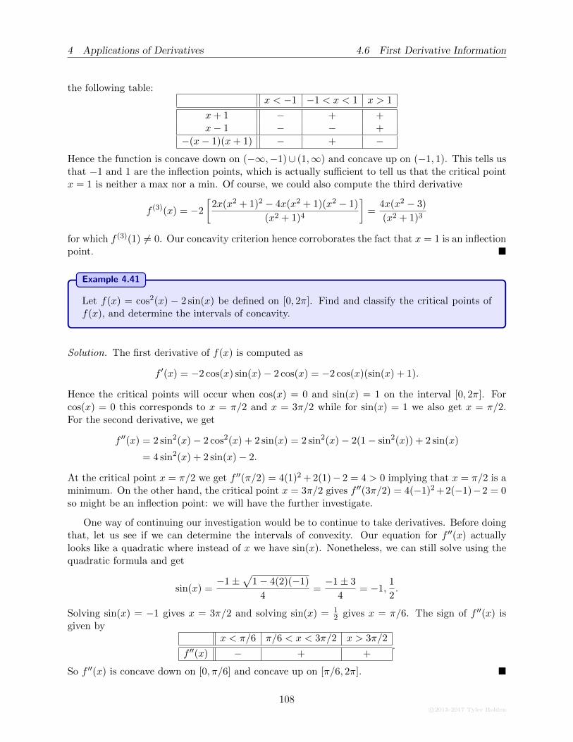
4 Applications of Derivatives 4.6 First Derivative Information
the following table:x < −1 −1 < x < 1 x > 1
x+ 1 − + +x− 1 − − +
−(x− 1)(x+ 1) − + −Hence the function is concave down on (−∞,−1)∪ (1,∞) and concave up on (−1, 1). This tells usthat −1 and 1 are the inflection points, which is actually sufficient to tell us that the critical pointx = 1 is neither a max nor a min. Of course, we could also compute the third derivative
f (3)(x) = −2
[2x(x2 + 1)2 − 4x(x2 + 1)(x2 − 1)
(x2 + 1)4
]=
4x(x2 − 3)
(x2 + 1)3
for which f (3)(1) 6= 0. Our concavity criterion hence corroborates the fact that x = 1 is an inflectionpoint. �
Example 4.41
Let f(x) = cos2(x) − 2 sin(x) be defined on [0, 2π]. Find and classify the critical points off(x), and determine the intervals of concavity.
Solution. The first derivative of f(x) is computed as
f ′(x) = −2 cos(x) sin(x)− 2 cos(x) = −2 cos(x)(sin(x) + 1).
Hence the critical points will occur when cos(x) = 0 and sin(x) = 1 on the interval [0, 2π]. Forcos(x) = 0 this corresponds to x = π/2 and x = 3π/2 while for sin(x) = 1 we also get x = π/2.For the second derivative, we get
f ′′(x) = 2 sin2(x)− 2 cos2(x) + 2 sin(x) = 2 sin2(x)− 2(1− sin2(x)) + 2 sin(x)
= 4 sin2(x) + 2 sin(x)− 2.
At the critical point x = π/2 we get f ′′(π/2) = 4(1)2 + 2(1)− 2 = 4 > 0 implying that x = π/2 is aminimum. On the other hand, the critical point x = 3π/2 gives f ′′(3π/2) = 4(−1)2 +2(−1)−2 = 0so might be an inflection point: we will have the further investigate.
One way of continuing our investigation would be to continue to take derivatives. Before doingthat, let us see if we can determine the intervals of convexity. Our equation for f ′′(x) actuallylooks like a quadratic where instead of x we have sin(x). Nonetheless, we can still solve using thequadratic formula and get
sin(x) =−1±
√1− 4(2)(−1)
4=−1± 3
4= −1,
1
2.
Solving sin(x) = −1 gives x = 3π/2 and solving sin(x) = 12 gives x = π/6. The sign of f ′′(x) is
given byx < π/6 π/6 < x < 3π/2 x > 3π/2
f ′′(x) − + +.
So f ′′(x) is concave down on [0, π/6] and concave up on [π/6, 2π]. �
108c©2013-2017 Tyler Holden

4.7 Maxima and Minima 4 Applications of Derivatives
Example 4.42
Consider the function f(x) =1 + x
1 + x2. Determine all inflection points of this curve.
Solution. We plug along until we get to the second derivative of f(x). The first derivative is givenby
f ′(x) =(1 + x2)− 2x(1 + x)
(1 + x2)= −x
2 + 2x− 1
x2 + 1,
while the second derivative is
f ′′(x) =(−2x− 2)(x2 + 1)2 − 4x(x2 + 1)(−x2 − 2x+ 1)
(x2 + 1)4=
2(x3 + 3x2 − 3x− 1)
(x2 + 1)3.
The inflection points come from finding the zeroes of the numerator. It is not too hard to see thatx = 1 is a zero, so we can factor this to get
x3 + 3x2 − 3x− 1 = (x− 1)(x2 + 4x+ 1)
and this second term has roots x = −2±√
3. It is not too hard to convince ourselves that these areinflection points (an easy argument comes from the fact that there are three distinct linear rootswith no multiplicities, hence the sign of the third derivative will change after passing any one root,implying each root is a proper inflection point). �
4.7 Maxima and Minima
This section describes one of the most important applications of calculus: the ability to find nec-essary conditions for a point to be an extreme point of a function. Solving such problems is ofexceptional importance. For example, all of classical mechanics works on the principle of leastaction: minimizing the difference between potential and kinetic energy. Relativity theory impliesthat gravity operates by moving particles along geodesics: paths of minimal length. When we sentpeople to the moon it was important to do it in the quickest amount of time while using the leastamount of fuel. In business, we often like to maximize profits while minimizing waste. So how doescalculus give us the ability to find extreme points? In order to make sense of this, we should firstdefine what it means to be a max/min!
Definition 4.43
Let f(x) be a function with domain D. We say that c is an absolute maximum if f(x) ≤ f(c)for all x ∈ D, and a local maximum if f(x) ≤ f(c) for all x in a interval around c. Similarly,we say that c is an absolute minimum if f(x) ≥ f(c) for all x ∈ D, and a local minimum iff(x) ≥ f(c) for all x in a interval around c.
Example 4.44
Find (in a hand-waving fashion) the absolute and local maxima and minima of the followingfunctions:
f(x) = x2, g(x) = cos(x), h(x) = x sin(x).
c©2013-2017 Tyler Holden
109
4 Applications of Derivatives 4.7 Maxima and Minima
Solution. Our intuition tells us that we should look at the plots of each of these functions. Noticethat f(x) = x2 has a global minimum at the point x = 0, but increases to infinity otherwise. Hencef(x) has a global min at x = 0 and no other extreme points.
The function g(x) = cos(x) has a global max wherever cos(x) = 1; that is, the points 2nπ for nan integer. Similarly, g(x) has a global min wherever cos(x) = −1, corresponding to the set
(2n+ 1)π where n is an integer.
Hence g(x) has multiple global maxima and minima.
Finally, if we look at the graph of the function h(x) = x sin(x) we see that there are manylocal maxima and minima, but as the amplitude of the function grows as |x| gets quite large, therecannot be any global max or min. �
Specifying the domain is very important. For example, the function f(x) = x has no global/localmaximum/minimum on R or (0, 1), but over the interval [0, 1] it has a minimum at x = 0 and amaximum at x = 1. The following useful theorem tells us that intervals of the form [a, b] ensurethat maxima and minima always exist:
Theorem 4.45: Extreme Value Theorem
If f(x) is a continuous function on a closed interval [a, b], then f(x) will attain its maximumand minimum on [a, b].
Example 4.46
Determine on which of the following intervals the function 1/x is guaranteed to attain itsglobal maximum and minimum.
[−1, 1], (0, 1), [1, 2].
Solution. According to the Extreme Value Theorem, we can be guaranteed that 1/x attains itsmax and min if it is continuous on a closed interval. The first interval [−1, 1] is closed but 1/xis not continuous at 0 which is a point in [−1, 1]. Hence we cannot guarantee that 1/x attains amax and min on [−1, 1], though note that it does attain global minima at x = ±1. Similarly, theinterval (0, 1) is not closed so we cannot guarantee that the maximum or minimum is attained. Infact, there is no max or min of 1/x in (0, 1). Finally, 1/x is continuous on [1, 2] and so by theExtreme Value Theorem the max and min are attained. �
This is all fine and dandy, but this is an existential theorem, meaning that it tells us whenextrema exist but fails to provide any information on how to find them. In fact, we notice that theExtreme Value Theorem only requires the concept of continuity and so does not really fall withinthe regime of calculus. The real power of calculus is to provide a necessary condition for a pointto be an extreme point.
110c©2013-2017 Tyler Holden
4.7 Maxima and Minima 4 Applications of Derivatives
Theorem 4.47
Let f(x) be a differentiable function on the interval [a, b]. If a < c < b is a local max or minof the function f(x), then it is a critical point of f(x).
The idea is that if a max/min occurs on the interior of the domain, then the function mustcurve back on itself. Think again of the function f(x) = x2 which we noticed had a minimum atx = 0. We could ensure it was a local min (and in fact a global on) because the function decreaseduntil it hit x = 0, then started to increase again. This means that at some point, the slope f ′(x)of the function must have been zero. Similarly, if the max/min occurs at the endpoint of a domainthen the derivative there did not exist.
Proof. If the domain of f(x) has endpoints and the max/min occur on the endpoints, then f ′(c)does not exist and we are done. Hence let us assume that c occurs inside the domain of f(x). Weshall proceed by showing the proof when c is a maximum value, and we claim that the proof whenc is a minimum value follows almost precisely the same logic.
Since c is a maximum value, we know that for all x in a neighbourhood of c that f(x) ≤ f(c). Inparticular, for sufficiently small h > 0 we have f(c+ h) ≤ f(c) or equivalently, f(c+ h)− f(c) ≤ 0.
Dividing by h we still get that f(c+h)−f(c)h ≤ 0 and taking the limit as h→ 0+, we get
limh→0+
f(c+ h)− f(c)
h≤ lim
h→0+0 = 0.
If we now let h < 0, then again f(c+ h)− f(c) ≤ 0, but this time dividing by h changes the sign.Taking the limit as h→ 0− gives
limh→0−
f(c+ h)− f(c)
h≥ lim
h→0−0 = 0.
Since the both one sided limits exist, the two sided limit also exists and we have
f ′(c) = limh→0
f(c+ h)− f(c)
h= 0.
As mentioned previously, the proof for when c is a local minimum proceeds in exactly the samemanner but with the inequalities reversed.
The idea behind why maxima and minima on the interior of the domain correspond to criticalpoints gives us the following test for maximality/minimality:
Theorem 4.48: First Derivative Test
Let f : [a, b]→ R be differentiable with critical point c ∈ (a, b).
1. If there exists δ > 0 such that f ′(x) > 0 on (c− δ, c) and f ′(x) < 0 on (c, c+ δ) then cis a maximum.
2. If there exists δ > 0 such that f ′(x) < 0 on (c− δ, c) and f ′(x) > 0 on (c, c+ δ) then cis a minimum.
c©2013-2017 Tyler Holden
111
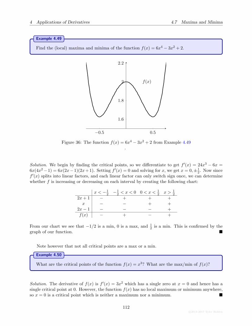
4 Applications of Derivatives 4.7 Maxima and Minima
Example 4.49
Find the (local) maxima and minima of the function f(x) = 6x4 − 3x2 + 2.
−0.5 0.5
1.6
1.8
2
2.2
f(x)
Figure 36: The function f(x) = 6x4 − 3x2 + 2 from Example 4.49.
Solution. We begin by finding the critical points, so we differentiate to get f ′(x) = 24x3 − 6x =6x(4x2−1) = 6x(2x− 1)(2x+ 1). Setting f ′(x) = 0 and solving for x, we get x = 0,±1
2 . Now sincef ′(x) splits into linear factors, and each linear factor can only switch sign once, we can determinewhether f is increasing or decreasing on each interval by creating the following chart:
x < −12 −1
2 < x < 0 0 < x < 12 x > 1
2
2x+ 1 − + + +x − − + +
2x− 1 − − − +
f(x) − + − +
From our chart we see that −1/2 is a min, 0 is a max, and 12 is a min. This is confirmed by the
graph of our function. �
Note however that not all critical points are a max or a min.
Example 4.50
What are the critical points of the function f(x) = x3? What are the max/min of f(x)?
Solution. The derivative of f(x) is f ′(x) = 3x2 which has a single zero at x = 0 and hence has asingle critical point at 0. However, the function f(x) has no local maximum or minimum anywhere,so x = 0 is a critical point which is neither a maximum nor a minimum. �
112c©2013-2017 Tyler Holden
4.7 Maxima and Minima 4 Applications of Derivatives
Theorem 4.47 combined with Example 4.50 imply that while every max/min is a critical point,not all critical points are max/mins. Regardless, critical points provide a powerful tools for findingabsolute maxima and minima. As we must also check whether the function achieves its max/minon the boundary, our strategy is as follows:
Finding Extreme Points
1. Determine the value of f(x) at the boundary points.
2. Determine the critical points of f(x) by computing the points where f ′(x) = 0.
3. Evaluate the function f(x) at its critical points.
4. The absolute max and min will be the largest and smallest values from steps (1) and(3).
Example 4.51
Determine the global maximum and minimum of the function f(x) = xe−x2
on the interval[0, 1].
Solution. Following our algorithm above, we first evaluate f(x) on its endpoints to find that
f(0) = 0, f(1) =1
e.
Next we determine the critical points: the derivative of f(x) is given by f ′(x) = e−x2(1−2x2). The
component e−x2
is never zero, so the zeroes of f ′(x) will occur precisely when 1 − 2x2 = 0 whichcorresponds to x = ±1/
√2. However, we notice that −1/
√2 is not in the interval [0, 1] so we throw
it away and just plug x = 1/√
2 into f(x) to get
f
(1√2
)=
1√2e−
12 =
1√2e.
A quick comparison tells us that f(0) < f(1) < f(1/√
2) so that 0 is the global minimum and 1/√
2is the global maximum. �
Example 4.52
Compute the global maximum and minimum of the function f(x) = x − arctan(x) on theinterval [−1, 1].
Solution. We recall that arctan(±1) = ±π4 , so that
f(−1) = −1 +π
4, f(1) = 1− π
4.
c©2013-2017 Tyler Holden
113
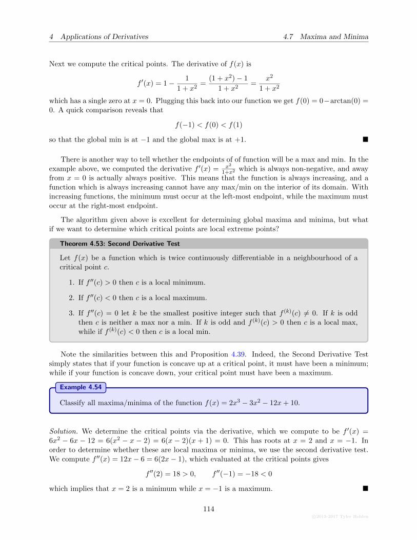
4 Applications of Derivatives 4.7 Maxima and Minima
Next we compute the critical points. The derivative of f(x) is
f ′(x) = 1− 1
1 + x2=
(1 + x2)− 1
1 + x2=
x2
1 + x2
which has a single zero at x = 0. Plugging this back into our function we get f(0) = 0−arctan(0) =0. A quick comparison reveals that
f(−1) < f(0) < f(1)
so that the global min is at −1 and the global max is at +1. �
There is another way to tell whether the endpoints of of function will be a max and min. In theexample above, we computed the derivative f ′(x) = x2
1+x2which is always non-negative, and away
from x = 0 is actually always positive. This means that the function is always increasing, and afunction which is always increasing cannot have any max/min on the interior of its domain. Withincreasing functions, the minimum must occur at the left-most endpoint, while the maximum mustoccur at the right-most endpoint.
The algorithm given above is excellent for determining global maxima and minima, but whatif we want to determine which critical points are local extreme points?
Theorem 4.53: Second Derivative Test
Let f(x) be a function which is twice continuously differentiable in a neighbourhood of acritical point c.
1. If f ′′(c) > 0 then c is a local minimum.
2. If f ′′(c) < 0 then c is a local maximum.
3. If f ′′(c) = 0 let k be the smallest positive integer such that f (k)(c) 6= 0. If k is oddthen c is neither a max nor a min. If k is odd and f (k)(c) > 0 then c is a local max,while if f (k)(c) < 0 then c is a local min.
Note the similarities between this and Proposition 4.39. Indeed, the Second Derivative Testsimply states that if your function is concave up at a critical point, it must have been a minimum;while if your function is concave down, your critical point must have been a maximum.
Example 4.54
Classify all maxima/minima of the function f(x) = 2x3 − 3x2 − 12x+ 10.
Solution. We determine the critical points via the derivative, which we compute to be f ′(x) =6x2 − 6x − 12 = 6(x2 − x − 2) = 6(x − 2)(x + 1) = 0. This has roots at x = 2 and x = −1. Inorder to determine whether these are local maxima or minima, we use the second derivative test.We compute f ′′(x) = 12x− 6 = 6(2x− 1), which evaluated at the critical points gives
f ′′(2) = 18 > 0, f ′′(−1) = −18 < 0
which implies that x = 2 is a minimum while x = −1 is a maximum. �
114c©2013-2017 Tyler Holden
4.7 Maxima and Minima 4 Applications of Derivatives
Example 4.55
Classify the maxima and minima of the function f(x) = x− sin(x).
Solution. The derivative f ′(x) is given by f ′(x) = 1− cos(x). Setting f ′(x) = 0 amounts to solvingcos(x) = 1 which occurs when x = 2nπ for n ∈ Z. In order to determine which of these aremaxima and which are minima, we compute the second derivative f ′′(x) = sin(x). Our goal is thusto determine the sign of sin(2nπ) for different integers n. However, it is easy to see that this isalways zero, so our second derivative test is at first indeterminate. The third derivative is given byf (3)(x) = − cos(x) and this is non-zero for every value of x = 2nπ. Since this occurred in the thirdderivative, our criterion above indicates that none of these points are maxima or minima. �
4.7.1 Optimization
Here we consider constrained optimization, where our goal is to maximize/minimize a functionsubject to constraints. There are entire fields of mathematics and engineering dedicated entirelyto the study of optimization. The principal difference between an optimization problem and amax/min problem is that optimization problems have constraints; that is, we are asked to find themaximize/minimize a quantity, but only so long as some other condition is satisfied. The additionof constraints typically makes the problem much more difficult (or if you’re a mathematician, muchmore interesting).
Keeping with the mathematical philosophy that one should reduce new problems to problemswhich we have already solved, our goal will be to take constrained optimization problems and turnthem into simple max/min problems. Typically, such questions will be posed as word-problemsamounting to the following
“Maximize f(x1, . . . , xn) subject to the constraint that g(x1, . . . , xn) = c.”
Written abstractly, this is guaranteed to terrify the student; how does one go about solving such asystem? Since this is only a single section in a course in single-variable calculus, it turns out thatthe constraint will almost always allow us rewrite f(x1, . . . , xn) as a function of a single variable,to which we can then apply our usual techniques. Let’s look at an example:
c©2013-2017 Tyler Holden
115
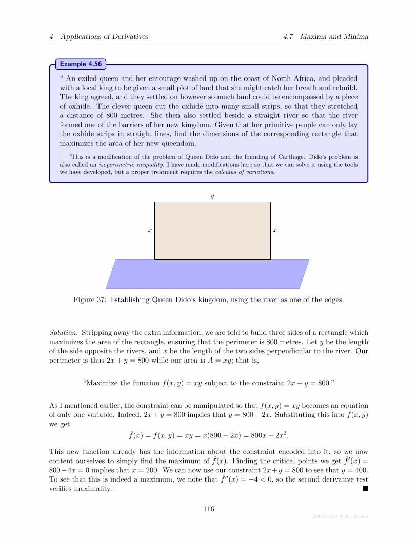
4 Applications of Derivatives 4.7 Maxima and Minima
Example 4.56
a An exiled queen and her entourage washed up on the coast of North Africa, and pleadedwith a local king to be given a small plot of land that she might catch her breath and rebuild.The king agreed, and they settled on however so much land could be encompassed by a pieceof oxhide. The clever queen cut the oxhide into many small strips, so that they stretcheda distance of 800 metres. She then also settled beside a straight river so that the riverformed one of the barriers of her new kingdom. Given that her primitive people can only laythe oxhide strips in straight lines, find the dimensions of the corresponding rectangle thatmaximizes the area of her new queendom.
aThis is a modification of the problem of Queen Dido and the founding of Carthage. Dido’s problem isalso called an isoperimetric inequality. I have made modifications here so that we can solve it using the toolswe have developed, but a proper treatment requires the calculus of variations.
x
y
x
Figure 37: Establishing Queen Dido’s kingdom, using the river as one of the edges.
Solution. Stripping away the extra information, we are told to build three sides of a rectangle whichmaximizes the area of the rectangle, ensuring that the perimeter is 800 metres. Let y be the lengthof the side opposite the rivers, and x be the length of the two sides perpendicular to the river. Ourperimeter is thus 2x+ y = 800 while our area is A = xy; that is,
“Maximize the function f(x, y) = xy subject to the constraint 2x+ y = 800.”
As I mentioned earlier, the constraint can be manipulated so that f(x, y) = xy becomes an equationof only one variable. Indeed, 2x+ y = 800 implies that y = 800− 2x. Substituting this into f(x, y)we get
f(x) = f(x, y) = xy = x(800− 2x) = 800x− 2x2.
This new function already has the information about the constraint encoded into it, so we nowcontent ourselves to simply find the maximum of f(x). Finding the critical points we get f ′(x) =800−4x = 0 implies that x = 200. We can now use our constraint 2x+y = 800 to see that y = 400.To see that this is indeed a maximum, we note that f ′′(x) = −4 < 0, so the second derivative testverifies maximality. �
116c©2013-2017 Tyler Holden
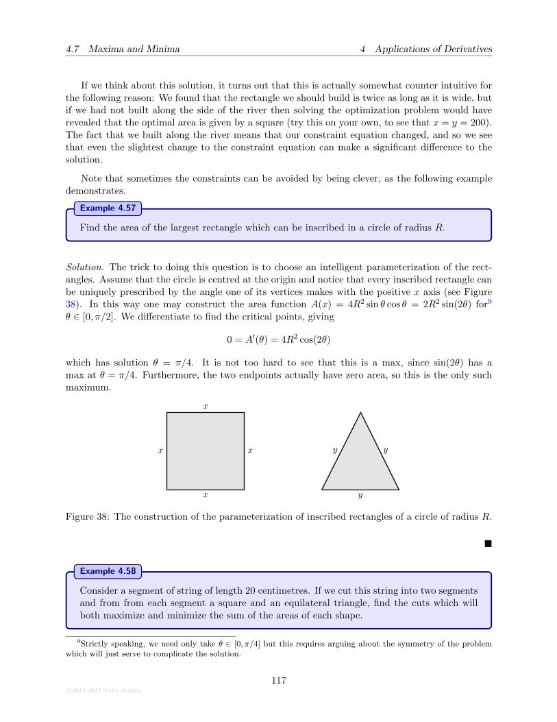
4.7 Maxima and Minima 4 Applications of Derivatives
If we think about this solution, it turns out that this is actually somewhat counter intuitive forthe following reason: We found that the rectangle we should build is twice as long as it is wide, butif we had not built along the side of the river then solving the optimization problem would haverevealed that the optimal area is given by a square (try this on your own, to see that x = y = 200).The fact that we built along the river means that our constraint equation changed, and so we seethat even the slightest change to the constraint equation can make a significant difference to thesolution.
Note that sometimes the constraints can be avoided by being clever, as the following exampledemonstrates.
Example 4.57
Find the area of the largest rectangle which can be inscribed in a circle of radius R.
Solution. The trick to doing this question is to choose an intelligent parameterization of the rect-angles. Assume that the circle is centred at the origin and notice that every inscribed rectangle canbe uniquely prescribed by the angle one of its vertices makes with the positive x axis (see Figure38). In this way one may construct the area function A(x) = 4R2 sin θ cos θ = 2R2 sin(2θ) for9
θ ∈ [0, π/2]. We differentiate to find the critical points, giving
0 = A′(θ) = 4R2 cos(2θ)
which has solution θ = π/4. It is not too hard to see that this is a max, since sin(2θ) has amax at θ = π/4. Furthermore, the two endpoints actually have zero area, so this is the only suchmaximum.
x
x
x
x
y
yy
Figure 38: The construction of the parameterization of inscribed rectangles of a circle of radius R.
�
Example 4.58
Consider a segment of string of length 20 centimetres. If we cut this string into two segmentsand from from each segment a square and an equilateral triangle, find the cuts which willboth maximize and minimize the sum of the areas of each shape.
9Strictly speaking, we need only take θ ∈ [0, π/4] but this requires arguing about the symmetry of the problemwhich will just serve to complicate the solution.
c©2013-2017 Tyler Holden
117
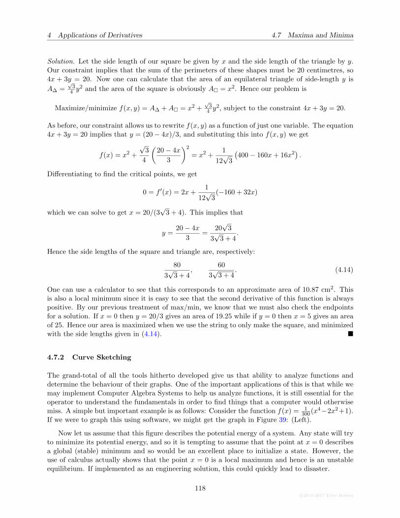
4 Applications of Derivatives 4.7 Maxima and Minima
Solution. Let the side length of our square be given by x and the side length of the triangle by y.Our constraint implies that the sum of the perimeters of these shapes must be 20 centimetres, so4x + 3y = 20. Now one can calculate that the area of an equilateral triangle of side-length y is
A∆ =√
34 y
2 and the area of the square is obviously A� = x2. Hence our problem is
Maximize/minimize f(x, y) = A∆ +A� = x2 +√
34 y
2, subject to the constraint 4x+ 3y = 20.
As before, our constraint allows us to rewrite f(x, y) as a function of just one variable. The equation4x+ 3y = 20 implies that y = (20− 4x)/3, and substituting this into f(x, y) we get
f(x) = x2 +
√3
4
(20− 4x
3
)2
= x2 +1
12√
3
(400− 160x+ 16x2
).
Differentiating to find the critical points, we get
0 = f ′(x) = 2x+1
12√
3(−160 + 32x)
which we can solve to get x = 20/(3√
3 + 4). This implies that
y =20− 4x
3=
20√
3
3√
3 + 4.
Hence the side lengths of the square and triangle are, respectively:
80
3√
3 + 4,
60
3√
3 + 4. (4.14)
One can use a calculator to see that this corresponds to an approximate area of 10.87 cm2. Thisis also a local minimum since it is easy to see that the second derivative of this function is alwayspositive. By our previous treatment of max/min, we know that we must also check the endpointsfor a solution. If x = 0 then y = 20/3 gives an area of 19.25 while if y = 0 then x = 5 gives an areaof 25. Hence our area is maximized when we use the string to only make the square, and minimizedwith the side lengths given in (4.14). �
4.7.2 Curve Sketching
The grand-total of all the tools hitherto developed give us that ability to analyze functions anddetermine the behaviour of their graphs. One of the important applications of this is that while wemay implement Computer Algebra Systems to help us analyze functions, it is still essential for theoperator to understand the fundamentals in order to find things that a computer would otherwisemiss. A simple but important example is as follows: Consider the function f(x) = 1
300(x4−2x2 +1).If we were to graph this using software, we might get the graph in Figure 39: (Left).
Now let us assume that this figure describes the potential energy of a system. Any state will tryto minimize its potential energy, and so it is tempting to assume that the point at x = 0 describesa global (stable) minimum and so would be an excellent place to initialize a state. However, theuse of calculus actually shows that the point x = 0 is a local maximum and hence is an unstableequilibrium. If implemented as an engineering solution, this could quickly lead to disaster.
118c©2013-2017 Tyler Holden
4.7 Maxima and Minima 4 Applications of Derivatives
−4 −2 2 4
200
400
−1.5 −1 −0.5 0.5 1 1.5
0.5
1.5
Figure 39: The graph of a misleading function. Left: The graph of our function as given by acomputer. Right: Zooming in, we see the presence of a local maximum at x = 0.
Our goal is thus to combine all of our information into a system which allows us to analyzethe qualitative behaviour of a function without knowing the nitty-gritty details of its exact valueat every point. There are approximately seven pieces of information that we need to compute toascertain the general behaviour.
1. Domain (and range of if possible),
2. Intercepts (x- and y-),
3. Symmetry (even/odd/none),
4. Asymptotes (horizontal/vertical/oblique),
5. Increasing (and obviously decreasing),
6. Maxima (and minima),
7. Concavity.
Of course, there is one piece of information above that I have not included; namely, what is anoblique (aka slant) asymptote?
Definition 4.59
Let f(x) and g(x) be continuous functions. We say that f(x) behaves like g(x) asymptoticallyif
limx→±∞
[f(x)− g(x)] = 0.
We say that f(x) has an oblique asymptote if f(x) behaves asymptotically like g(x) = mx+bfor some m 6= 0.
c©2013-2017 Tyler Holden
119
4 Applications of Derivatives 4.7 Maxima and Minima
Example 4.60
Compute any asymptotics of the function f(x) =2x3 − x2 + 2x
x2 + 1.
Solution. The easiest way to proceed is to try to write f(x) as an improper rational function.Performing long division, we see that
f(x) = (2x− 1) +1
x2 + 1.
The idea is that in the limit as x→∞, then 1/(x2 + 1) term will die off and contribute very littleto the behaviour of f(x), so that f(x) looks like the function 2x− 1. To see that this satisfies thedefinition above, set g(x) = 2x− 1 so that
limx→∞
[f(x)− g(x)] = limx→∞
[2x− 1 +
1
x2 + 1− (2x− 1)
]
= limx→∞
1
x2 + 1= 0,
which is precisely what we wanted to show. Similarly, the limit as x→ −∞ shows that f(x) is alsoasymptotically like g(x) in that limit as well. Thus 2x− 1 is an oblique asymptote for f(x) at both±∞. �
Now that we know how to compute all terms involved in this computation, we shall proceedwith some examples.
Example 4.61
Plot the function f(x) =x3
(x+ 1)2.
Solution. Domain: The only point which could possibly give us trouble is x = −1. Hence ourdomain is simply R \ {−1}.
Intercepts: The y-intercept occurs when x = 0, so namely f(0) = 0. Similarly the x-interceptcomes when y = 0, for which we see that
x3
(x+ 1)2= 0, ⇔ x = 0.
Thus the x- and y-intercepts both occur at the origin.
Symmetry: There is no symmetry involved: Since the functions are polynomial they have noperiodicity. The student may check that f(−x) has no relation to f(x), so that the function isneither even nor odd.
Asymptotes: We begin with the horizontal asymptotes. It is easy to see that since thenumerator dominates the denominator, the limit will go to infinity (check this by dividing top and
120c©2013-2017 Tyler Holden
4.7 Maxima and Minima 4 Applications of Derivatives
bottom by 1/x3). Further, since the denominator is always positive, the sign is determined entirelyby the x3 factor, so
limx→∞
x3
(x+ 1)2=∞, lim
x→−∞
x3
(x+ 1)2= −∞.
We conclude there are no horizontal asymptotes.
The only candidate for a vertical asymptote occurs at x = −1. Again the denominator (x+ 1)2
is always positive, so the sign of the “infinity” is entirely determined by the behaviour of x3 aroundx = −1, which is negative. It is then clear that
limx→1±
x3
(x+ 1)2= −∞.
Finally, we want to check for oblique asymptotes. Using long polynomial division we may easilyfind that
x3
(x+ 1)2= (x− 2) +
3x+ 2
x2 + 2x+ 1
so we claim that y = x− 2 is an oblique asymptote. Indeed, notice that
limx→±∞
[f(x)− (x− 2)] = limx→±∞
[((x− 2)− 3x+ 2
x2 + 2x+ 1
)− (x− 2)
]
= − limx→±∞
3x+ 2
x2 + 2x+ 1
= − limx→±∞
3/x + 2/x2
1 + 2/x + 1/x2multiply and
divide by 1/x2.
= 0.
First Derivative: Computing the first derivative can be a chore, but we find that
f ′(x) =3x2(x+ 1)2 − 2(x+ 1)x3
(x+ 1)4
=3x4 + 6x3 + 3x2 − 2x4 − 2x3
(x+ 1)4
=x2(x+ 3)(x+ 1)
(x+ 1)4
=x2(x+ 3)
(x+ 1)3
so that the critical points correspond to x = −1, x = 0 and x = −3. The y-values for these pointswill be useful when we plot, so we substitute to find that f(0) = 0 and f(−3) = 27/16. To determinewhere the function is increasing and decreasing, we consider the following table:
x < −3 −3 < x < −1 −1 < x < 0 0 < x
x+ 3 − + + +
(x+ 1)3 − − + +
x2 + + + +
f(x) + − + +
c©2013-2017 Tyler Holden
121
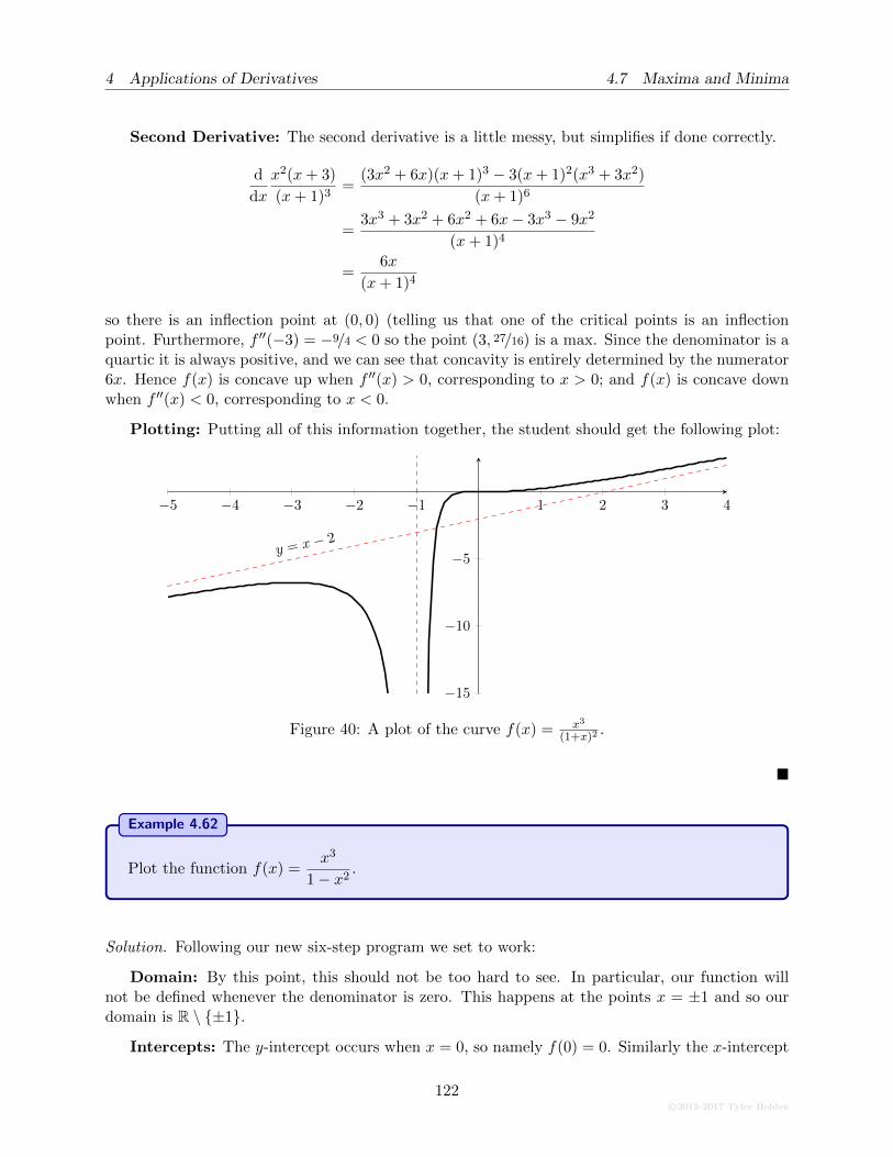
4 Applications of Derivatives 4.7 Maxima and Minima
Second Derivative: The second derivative is a little messy, but simplifies if done correctly.
d
dx
x2(x+ 3)
(x+ 1)3=
(3x2 + 6x)(x+ 1)3 − 3(x+ 1)2(x3 + 3x2)
(x+ 1)6
=3x3 + 3x2 + 6x2 + 6x− 3x3 − 9x2
(x+ 1)4
=6x
(x+ 1)4
so there is an inflection point at (0, 0) (telling us that one of the critical points is an inflectionpoint. Furthermore, f ′′(−3) = −9/4 < 0 so the point (3, 27/16) is a max. Since the denominator is aquartic it is always positive, and we can see that concavity is entirely determined by the numerator6x. Hence f(x) is concave up when f ′′(x) > 0, corresponding to x > 0; and f(x) is concave downwhen f ′′(x) < 0, corresponding to x < 0.
Plotting: Putting all of this information together, the student should get the following plot:
−5 −4 −3 −2 −1 1 2 3 4
−15
−10
−5y = x− 2
Figure 40: A plot of the curve f(x) = x3
(1+x)2.
�
Example 4.62
Plot the function f(x) =x3
1− x2.
Solution. Following our new six-step program we set to work:
Domain: By this point, this should not be too hard to see. In particular, our function willnot be defined whenever the denominator is zero. This happens at the points x = ±1 and so ourdomain is R \ {±1}.
Intercepts: The y-intercept occurs when x = 0, so namely f(0) = 0. Similarly the x-intercept
122c©2013-2017 Tyler Holden
4.7 Maxima and Minima 4 Applications of Derivatives
comes when y = 0, for which we see that
x3
1− x2= 0, ⇔ x = 0.
Thus the x- and y-intercepts both occur at the origin.
Symmetry: Since we are dealing with polynomials, there is no obvious periodicity to worryabout. It’s not too hard to see that this is actually an odd function, since
f(−x) =(−x)3
1− (−x)2= − x3
1− x2= −f(x).
Asymptotes: The vertical asymptotes will clearly occur at x = ±1. Typically, one wouldcalculate the limits
limx→1±
x3
1− x2, lim
x→−1±
x3
1− x2
but this is laborious and is redundant once we have information on the first derivative. For theinterested student who would like to see how to do this all the same, we have the following table
x3 1− x2 x3/1−x2
x→ 1+ + − −x→ 1− + + +
x→ −1+ − + −x→ −1− − − +
so that
limx→1−
x3
1− x2= lim
x→−1−
x3
1− x2=∞, lim
x→1+
x3
1− x2= lim
x→−1+
x3
1− x2=∞
Because the degree of the numerator is strictly greater than the degree of the denominator,there are no horizontal asymptotes:
limx→±∞
x3
1− x2= ∓∞.
Finally, we want to check for oblique asymptotes. Using long polynomial division we may easilyfind that
x3
1− x2= −x+
x
1− x2
so we claim that y = −x is an oblique asymptote. Indeed, notice that
limx→±∞
[f(x)− (−x)] = limx→±∞
[x3
1− x2+ x
]
= limx→±∞
x
1− x2
= limx→±∞
1/x1/x2 − 1
= 0.
c©2013-2017 Tyler Holden
123
4 Applications of Derivatives 4.7 Maxima and Minima
First Derivative: This step allows us to determine where the function is increasing, decreasing,the critical points, and when combined with the second derivative, maxima and minima. The firstderivative is computed to be
d
dx
x3
1− x2=
(3x2)(1− x2)− (−2x)(x3)
(1− x2)2
=x2(3− x2)
(1− x2)2.
We may simply read off the critical points as{±1,±
√3, 0}
with potential extrema at{
0,±√
3}
.Setting up a quick table for increasing and decreasing we have
x < −√
3 −√
3 < x < −1 −1 < x < 0 0 < x < −1 1 < x <√
3 x >√
3
f(x) − + + + + −
This table is easy to deduce once we realize that the x2
(1−x2)2portion is always positive, so the sign
of f ′(x) is entirely determined by the sign of 3− x2, which is negative whenever |x| >√
3. It willlikely be useful to know the function values corresponding to our critical points. We already knowthat f(0) = 0 and we find that
f(±√
3) =±3√
3
−2=∓3√
3
2.
Second Derivative: The second derivative is a little messy, but simplifies if done correctly.
d
dx
x2(3− x2)
(1− x2)2=
(6x− 4x3)(1− x)2 − 2(1− x2)(−2x)(3x3 − x4)
(1− x2)4
=2x(x2 + 3)
(1− x2)3.
The inflection points will occur when f ′′(x) = 0 or does not exist, which we can again read offas being {0,±1}. We form a table to check for concavity and find
x < −1 −1 < x < 0 0 < x < 1 x > 1
f(x) + − + −
Finally, recalling that we have extrema candidate at ±3 we check to find that
f(±√
3) =±2√
3(3 + 3)
(1− 3)2= ±12
√3
−8= ∓3
√3
2.
Thus(√
3,−3√
32
)is a local maximum and
(−√
3, 3√
32
)is a local minimum. Since f ′′(0) = 0 we
cannot infer any information about this critical point. If we continue to take derivatives, we willfind that f (3)(0) = 6 and so by the generalized second derivative test, 0 is an inflection point.
Plotting: Putting all of this information together, the student should get the following plot:
�
124c©2013-2017 Tyler Holden
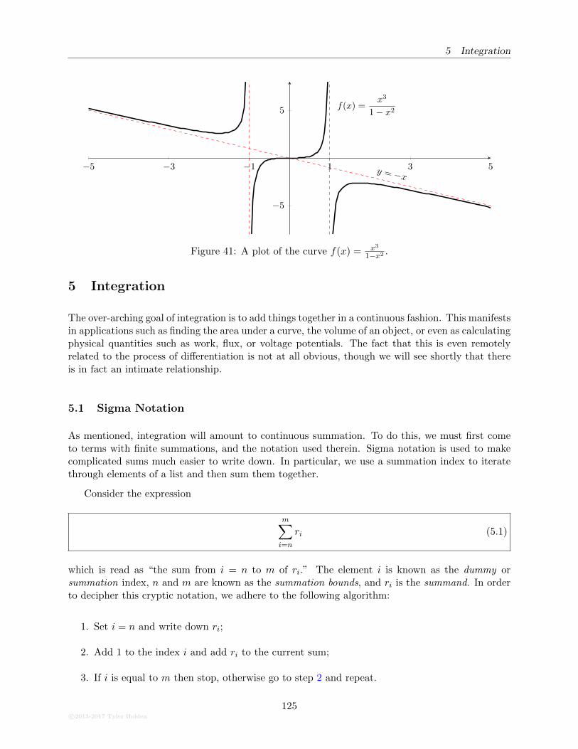
5 Integration
−5 −3 −1 1 3 5
−5
5f(x) =
x3
1− x2
y = −x
Figure 41: A plot of the curve f(x) = x3
1−x2 .
5 Integration
The over-arching goal of integration is to add things together in a continuous fashion. This manifestsin applications such as finding the area under a curve, the volume of an object, or even as calculatingphysical quantities such as work, flux, or voltage potentials. The fact that this is even remotelyrelated to the process of differentiation is not at all obvious, though we will see shortly that thereis in fact an intimate relationship.
5.1 Sigma Notation
As mentioned, integration will amount to continuous summation. To do this, we must first cometo terms with finite summations, and the notation used therein. Sigma notation is used to makecomplicated sums much easier to write down. In particular, we use a summation index to iteratethrough elements of a list and then sum them together.
Consider the expression
m∑
i=n
ri (5.1)
which is read as “the sum from i = n to m of ri.” The element i is known as the dummy orsummation index, n and m are known as the summation bounds, and ri is the summand. In orderto decipher this cryptic notation, we adhere to the following algorithm:
1. Set i = n and write down ri;
2. Add 1 to the index i and add ri to the current sum;
3. If i is equal to m then stop, otherwise go to step 2 and repeat.
c©2013-2017 Tyler Holden
125
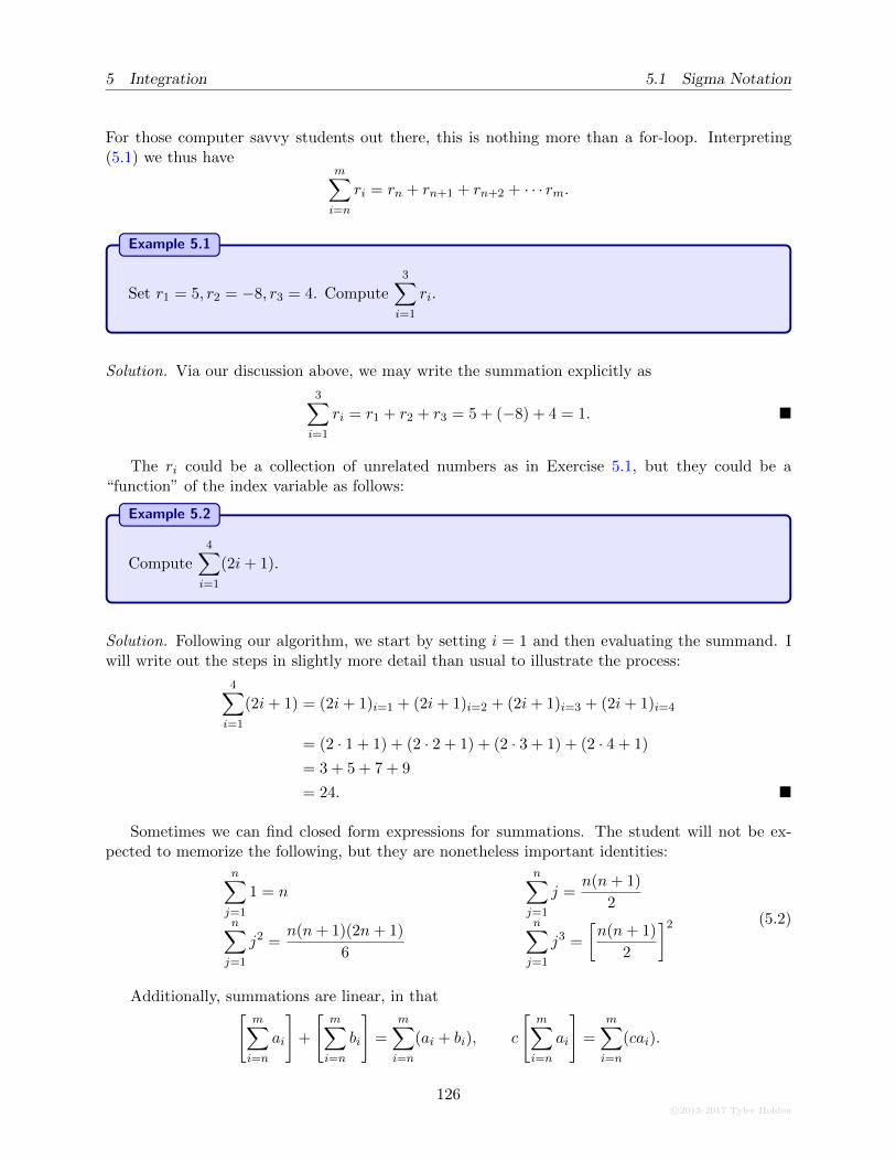
5 Integration 5.1 Sigma Notation
For those computer savvy students out there, this is nothing more than a for-loop. Interpreting(5.1) we thus have
m∑
i=n
ri = rn + rn+1 + rn+2 + · · · rm.
Example 5.1
Set r1 = 5, r2 = −8, r3 = 4. Compute
3∑
i=1
ri.
Solution. Via our discussion above, we may write the summation explicitly as
3∑
i=1
ri = r1 + r2 + r3 = 5 + (−8) + 4 = 1. �
The ri could be a collection of unrelated numbers as in Exercise 5.1, but they could be a“function” of the index variable as follows:
Example 5.2
Compute4∑
i=1
(2i+ 1).
Solution. Following our algorithm, we start by setting i = 1 and then evaluating the summand. Iwill write out the steps in slightly more detail than usual to illustrate the process:
4∑
i=1
(2i+ 1) = (2i+ 1)i=1 + (2i+ 1)i=2 + (2i+ 1)i=3 + (2i+ 1)i=4
= (2 · 1 + 1) + (2 · 2 + 1) + (2 · 3 + 1) + (2 · 4 + 1)
= 3 + 5 + 7 + 9
= 24. �
Sometimes we can find closed form expressions for summations. The student will not be ex-pected to memorize the following, but they are nonetheless important identities:
n∑
j=1
1 = nn∑
j=1
j =n(n+ 1)
2n∑
j=1
j2 =n(n+ 1)(2n+ 1)
6
n∑
j=1
j3 =
[n(n+ 1)
2
]2 (5.2)
Additionally, summations are linear, in that[m∑
i=n
ai
]+
[m∑
i=n
bi
]=
m∑
i=n
(ai + bi), c
[m∑
i=n
ai
]=
m∑
i=n
(cai).
126c©2013-2017 Tyler Holden
5.1 Sigma Notation 5 Integration
Note that the upper and lower bounds of the summation are the same in every summation.
Using linearity and the identities in (5.2) we can redo Example 5.2 with a general upper bound,to find
n∑
i=1
(2i+ 1) = 2
(n∑
i=1
i
)+
(n∑
i=1
1
)
= 2n(n+ 1)
2+ n
= n(n+ 2).
Plugging in n = 4 we get 24, just as we found in Example 5.2.
Remark 5.3 For any positive integer p, there is a closed form expression for
n∑
i=1
ip
but these expressions become more difficult as p becomes larger. Luckily, there is a standardway of deriving the closed form for any p using the Bernoulli polynomials, which are popularobjects in the study of number theory but are tricky to define.
There are other summations which also admit closed form expressions, which are not evaluatedas easily as the examples above.
Example 5.4
Guess a closed form expression for the summation
n∑
i=1
1
i2 + i.
Solution. We will try a few values of n, such as n = 1, 2, 3, 4; to see if we can spot a pattern.Indeed,
n = 1 :1∑
i=1
1
i2 + i=
1
2
n = 2 :
2∑
i=1
1
i2 + i=
1
2+
1
6=
2
3
n = 3 :
3∑
i=1
1
i2 + i=
2
3+
1
12=
3
4
n = 4 :4∑
i=1
1
i2 + i=
3
4+
1
20=
4
5.
Were we to guess, it looks as though
n∑
i=1
1
i2 + i=
n
n+ 1, (5.3)
c©2013-2017 Tyler Holden
127
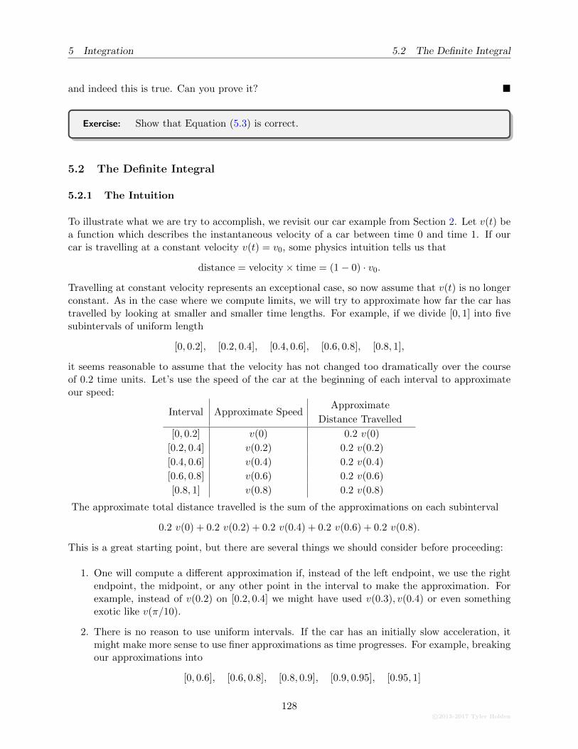
5 Integration 5.2 The Definite Integral
and indeed this is true. Can you prove it? �
Exercise: Show that Equation (5.3) is correct.
5.2 The Definite Integral
5.2.1 The Intuition
To illustrate what we are try to accomplish, we revisit our car example from Section 2. Let v(t) bea function which describes the instantaneous velocity of a car between time 0 and time 1. If ourcar is travelling at a constant velocity v(t) = v0, some physics intuition tells us that
distance = velocity× time = (1− 0) · v0.
Travelling at constant velocity represents an exceptional case, so now assume that v(t) is no longerconstant. As in the case where we compute limits, we will try to approximate how far the car hastravelled by looking at smaller and smaller time lengths. For example, if we divide [0, 1] into fivesubintervals of uniform length
[0, 0.2], [0.2, 0.4], [0.4, 0.6], [0.6, 0.8], [0.8, 1],
it seems reasonable to assume that the velocity has not changed too dramatically over the courseof 0.2 time units. Let’s use the speed of the car at the beginning of each interval to approximateour speed:
Interval Approximate SpeedApproximate
Distance Travelled
[0, 0.2] v(0) 0.2 v(0)
[0.2, 0.4] v(0.2) 0.2 v(0.2)
[0.4, 0.6] v(0.4) 0.2 v(0.4)
[0.6, 0.8] v(0.6) 0.2 v(0.6)
[0.8, 1] v(0.8) 0.2 v(0.8)
The approximate total distance travelled is the sum of the approximations on each subinterval
0.2 v(0) + 0.2 v(0.2) + 0.2 v(0.4) + 0.2 v(0.6) + 0.2 v(0.8).
This is a great starting point, but there are several things we should consider before proceeding:
1. One will compute a different approximation if, instead of the left endpoint, we use the rightendpoint, the midpoint, or any other point in the interval to make the approximation. Forexample, instead of v(0.2) on [0.2, 0.4] we might have used v(0.3), v(0.4) or even somethingexotic like v(π/10).
2. There is no reason to use uniform intervals. If the car has an initially slow acceleration, itmight make more sense to use finer approximations as time progresses. For example, breakingour approximations into
[0, 0.6], [0.6, 0.8], [0.8, 0.9], [0.9, 0.95], [0.95, 1]
128c©2013-2017 Tyler Holden
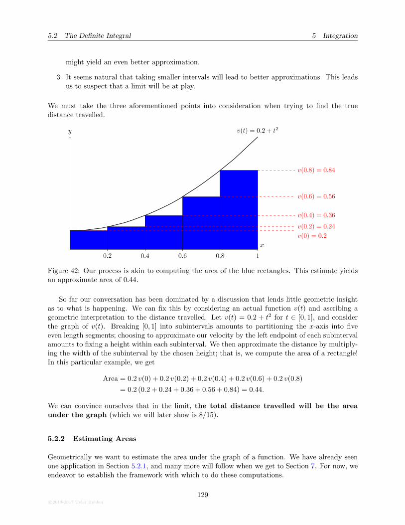
5.2 The Definite Integral 5 Integration
might yield an even better approximation.
3. It seems natural that taking smaller intervals will lead to better approximations. This leadsus to suspect that a limit will be at play.
We must take the three aforementioned points into consideration when trying to find the truedistance travelled.
0.2 0.4 0.6 0.8 1
v(0.2) = 0.24
v(0.4) = 0.36
v(0.6) = 0.56
v(0.8) = 0.84
v(0) = 0.2
x
y v(t) = 0.2 + t2
Figure 42: Our process is akin to computing the area of the blue rectangles. This estimate yieldsan approximate area of 0.44.
So far our conversation has been dominated by a discussion that lends little geometric insightas to what is happening. We can fix this by considering an actual function v(t) and ascribing ageometric interpretation to the distance travelled. Let v(t) = 0.2 + t2 for t ∈ [0, 1], and considerthe graph of v(t). Breaking [0, 1] into subintervals amounts to partitioning the x-axis into fiveeven length segments; choosing to approximate our velocity by the left endpoint of each subintervalamounts to fixing a height within each subinterval. We then approximate the distance by multiply-ing the width of the subinterval by the chosen height; that is, we compute the area of a rectangle!In this particular example, we get
Area = 0.2 v(0) + 0.2 v(0.2) + 0.2 v(0.4) + 0.2 v(0.6) + 0.2 v(0.8)
= 0.2 (0.2 + 0.24 + 0.36 + 0.56 + 0.84) = 0.44.
We can convince ourselves that in the limit, the total distance travelled will be the areaunder the graph (which we will later show is 8/15).
5.2.2 Estimating Areas
Geometrically we want to estimate the area under the graph of a function. We have already seenone application in Section 5.2.1, and many more will follow when we get to Section 7. For now, weendeavor to establish the framework with which to do these computations.
c©2013-2017 Tyler Holden
129
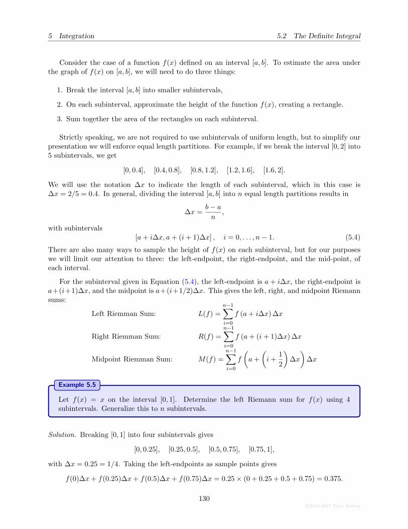
5 Integration 5.2 The Definite Integral
Consider the case of a function f(x) defined on an interval [a, b]. To estimate the area underthe graph of f(x) on [a, b], we will need to do three things:
1. Break the interval [a, b] into smaller subintervals,
2. On each subinterval, approximate the height of the function f(x), creating a rectangle.
3. Sum together the area of the rectangles on each subinterval.
Strictly speaking, we are not required to use subintervals of uniform length, but to simplify ourpresentation we will enforce equal length partitions. For example, if we break the interval [0, 2] into5 subintervals, we get
[0, 0.4], [0.4, 0.8], [0.8, 1.2], [1.2, 1.6], [1.6, 2].
We will use the notation ∆x to indicate the length of each subinterval, which in this case is∆x = 2/5 = 0.4. In general, dividing the interval [a, b] into n equal length partitions results in
∆x =b− an
,
with subintervals[a+ i∆x, a+ (i+ 1)∆x] , i = 0, . . . , n− 1. (5.4)
There are also many ways to sample the height of f(x) on each subinterval, but for our purposeswe will limit our attention to three: the left-endpoint, the right-endpoint, and the mid-point, ofeach interval.
For the subinterval given in Equation (5.4), the left-endpoint is a+ i∆x, the right-endpoint isa+(i+1)∆x, and the midpoint is a+(i+1/2)∆x. This gives the left, right, and midpoint Riemannsums:
Left Riemman Sum: L(f) =n−1∑
i=0
f (a+ i∆x) ∆x
Right Riemman Sum: R(f) =
n−1∑
i=0
f (a+ (i+ 1)∆x) ∆x
Midpoint Riemman Sum: M(f) =
n−1∑
i=0
f
(a+
(i+
1
2
)∆x
)∆x
Example 5.5
Let f(x) = x on the interval [0, 1]. Determine the left Riemann sum for f(x) using 4subintervals. Generalize this to n subintervals.
Solution. Breaking [0, 1] into four subintervals gives
[0, 0.25], [0.25, 0.5], [0.5, 0.75], [0.75, 1],
with ∆x = 0.25 = 1/4. Taking the left-endpoints as sample points gives
f(0)∆x+ f(0.25)∆x+ f(0.5)∆x+ f(0.75)∆x = 0.25× (0 + 0.25 + 0.5 + 0.75) = 0.375.
130c©2013-2017 Tyler Holden
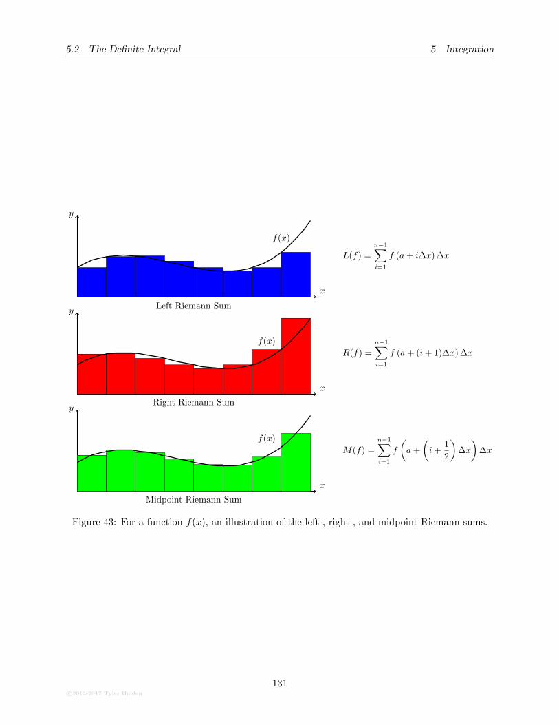
5.2 The Definite Integral 5 Integration
x
y
Left Riemann Sum
f(x)
L(f) =
n−1∑
i=1
f (a+ i∆x) ∆x
x
y
Right Riemann Sum
f(x)
R(f) =
n−1∑
i=1
f (a+ (i+ 1)∆x) ∆x
x
y
Midpoint Riemann Sum
f(x)
M(f) =
n−1∑
i=1
f
(a+
(i+
1
2
)∆x
)∆x
Figure 43: For a function f(x), an illustration of the left-, right-, and midpoint-Riemann sums.
c©2013-2017 Tyler Holden
131
5 Integration 5.2 The Definite Integral
More generally, when we have n subintervals the length of each partition is ∆x = 1/n and oursubintervals are of the form [
i
n,(i+ 1)
n
].
The left Riemann sum is thus
L(f) =n−1∑
i=0
f
(i
n
)∆x =
1
n
n−1∑
i=0
i
n=
1
n2
n(n− 1)
2=n− 1
2n. �
Example 5.6
Let f(x) = x2 on [1, 4]. Determine the right Riemann sum for f(x) using three subintervals.Generalize this to n subintervals.
Solution. Breaking [1, 4] into three subintervals gives
[1, 2], [2, 3], [3, 4],
with ∆x = 1. Thus the right Riemann sum is
f(2)∆x+ f(3)∆x+ f(4)∆x = 1× (4 + 9 + 16) = 29.
More generally, when we have n subinterval the length of each partition is ∆x = (4− 1)/n = 3/nand our subintervals are of the form
[1 +
3i
n, 1 +
3(i+ 1)
n
].
Thus the right Riemann sum is
R(f) =
n−1∑
i=0
f
(1 +
3(i+ 1)
n
)∆x =
3
n
n∑
i=0
(1 +
3(i+ 1)
n
)2
=3
n
n−1∑
i=0
[1 +
6(i+ 1)
n+
9(i+ 1)2
n2
]. (5.5)
This expression can be simplified further, but we won’t worry about that. �
Exercise: Simplify (5.5) using (5.2).
5.2.3 Defining the Definite Integral
We really want to know the exact area under a curve, not just an approximation. With theidea that taking a larger number of subintervals in our estimate should result in a more accurateapproximation to the area, we are lead to the definition of the definite integral.
132c©2013-2017 Tyler Holden
5.2 The Definite Integral 5 Integration
Definition 5.7
Let f(x) be a function defined on [a, b]. For a positive integer n, let ∆x = (b− a)/n and xibe any point in the interval [a+ i∆x, a+ (i+ 1)∆x]. We say that f is integrable if
∫ b
af(x) dx := lim
n→∞
n−1∑
i=0
f(xi)∆x
exists. When this limit exists, we say that∫ ba f(x) dx is the definite integral of f(x).
Important in this definition is that if f(x) is integrable, the choice of the points xi do not matter.Hence we may choose the left, right, midpoint, or any other Riemann sum we like to evaluate thedefinite integral.
While we will not prove it, any function which is continuous is integrable. In fact, any functionthat has finitely many discontinuities is integrable. We will assume this result henceforth.
Example 5.8
Determine the value of
∫ 1
0x dx. More generally, what is the value of
∫ b
ax dx?
Solution. We showed in Example 5.5 that the left Riemann sum for f(x) = x over the interval [0, 1]is given by
L =
n−1∑
i=0
f
(i
n
)∆x =
n− 1
2n.
Taking the limit as n→∞ gives
∫ 1
0x dx = lim
n→∞
n− 1
2n=
1
2.
More generally, since f is continuous it is integrable. The left Riemann sum is
L(f) =b− an
n−1∑
i=0
f
(a+ i
(b− an
))
=b− an
n−1∑
i=0
[a+ i
(b− an
)]
=b− an
[a
(n−1∑
i=0
1
)+b− an
(n−1∑
i=0
i
)]
=b− an
[an+ (b− a)
n− 1
2
]
= (ab− a2) + (b− a)2
(n− 1
2n
).
c©2013-2017 Tyler Holden
133
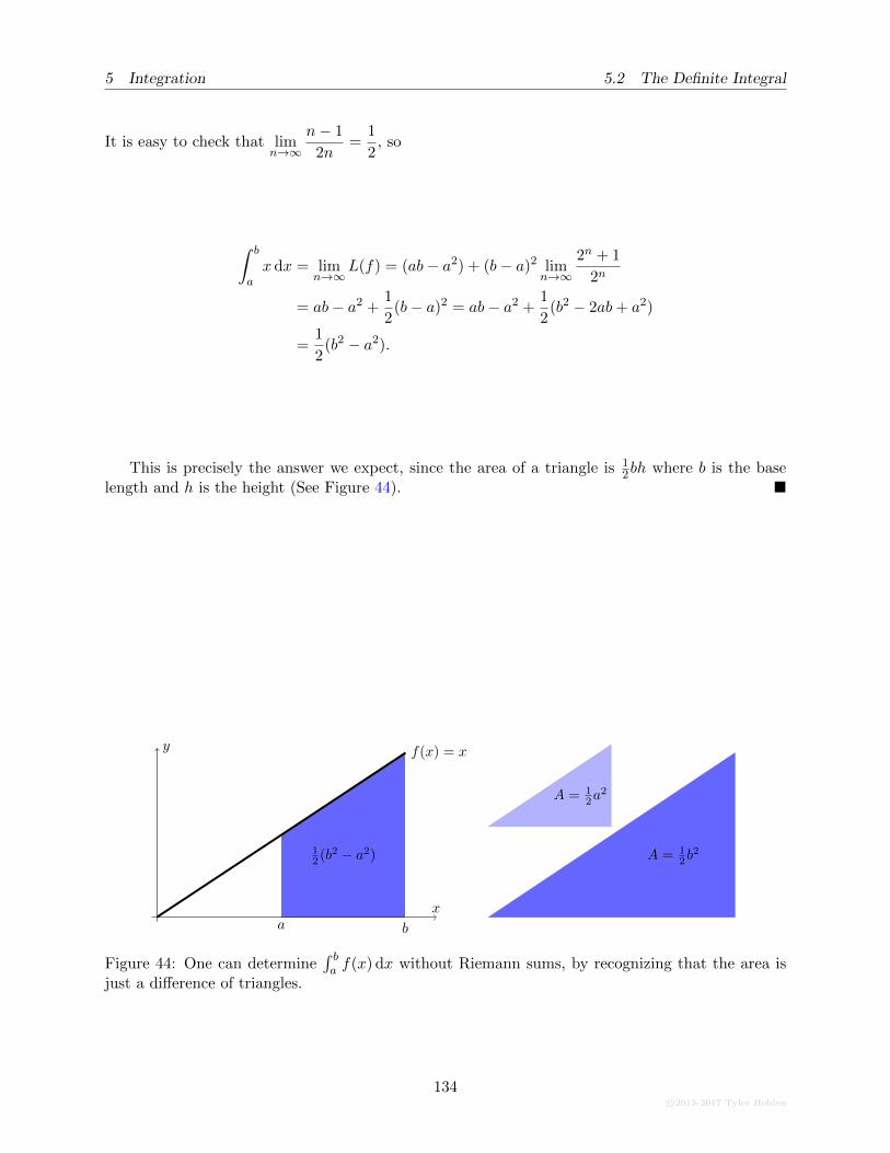
5 Integration 5.2 The Definite Integral
It is easy to check that limn→∞
n− 1
2n=
1
2, so
∫ b
ax dx = lim
n→∞L(f) = (ab− a2) + (b− a)2 lim
n→∞
2n + 1
2n
= ab− a2 +1
2(b− a)2 = ab− a2 +
1
2(b2 − 2ab+ a2)
=1
2(b2 − a2).
This is precisely the answer we expect, since the area of a triangle is 12bh where b is the base
length and h is the height (See Figure 44). �
a b
f(x) = x
x
y
12 (b
2 − a2) A = 12b
2
A = 12a
2
Figure 44: One can determine∫ ba f(x) dx without Riemann sums, by recognizing that the area is
just a difference of triangles.
134c©2013-2017 Tyler Holden
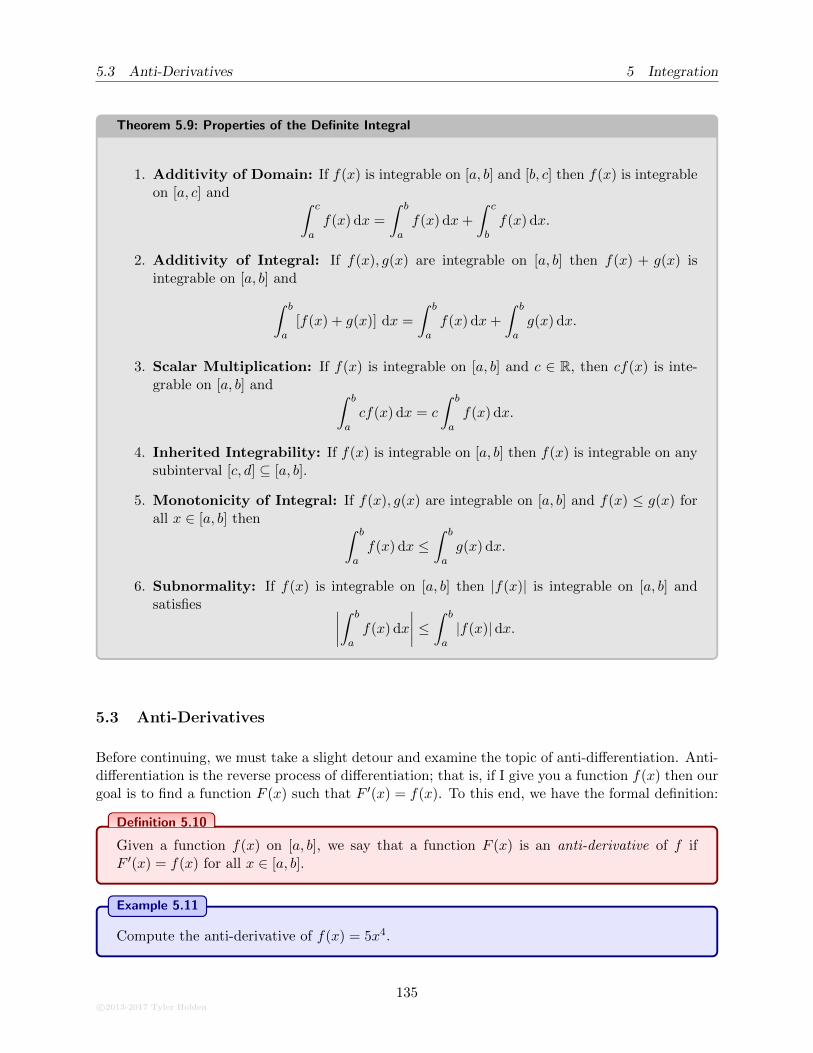
5.3 Anti-Derivatives 5 Integration
Theorem 5.9: Properties of the Definite Integral
1. Additivity of Domain: If f(x) is integrable on [a, b] and [b, c] then f(x) is integrableon [a, c] and ∫ c
af(x) dx =
∫ b
af(x) dx+
∫ c
bf(x) dx.
2. Additivity of Integral: If f(x), g(x) are integrable on [a, b] then f(x) + g(x) isintegrable on [a, b] and
∫ b
a[f(x) + g(x)] dx =
∫ b
af(x) dx+
∫ b
ag(x) dx.
3. Scalar Multiplication: If f(x) is integrable on [a, b] and c ∈ R, then cf(x) is inte-grable on [a, b] and ∫ b
acf(x) dx = c
∫ b
af(x) dx.
4. Inherited Integrability: If f(x) is integrable on [a, b] then f(x) is integrable on anysubinterval [c, d] ⊆ [a, b].
5. Monotonicity of Integral: If f(x), g(x) are integrable on [a, b] and f(x) ≤ g(x) forall x ∈ [a, b] then ∫ b
af(x) dx ≤
∫ b
ag(x) dx.
6. Subnormality: If f(x) is integrable on [a, b] then |f(x)| is integrable on [a, b] andsatisfies ∣∣∣∣
∫ b
af(x) dx
∣∣∣∣ ≤∫ b
a|f(x)|dx.
5.3 Anti-Derivatives
Before continuing, we must take a slight detour and examine the topic of anti-differentiation. Anti-differentiation is the reverse process of differentiation; that is, if I give you a function f(x) then ourgoal is to find a function F (x) such that F ′(x) = f(x). To this end, we have the formal definition:
Definition 5.10
Given a function f(x) on [a, b], we say that a function F (x) is an anti-derivative of f ifF ′(x) = f(x) for all x ∈ [a, b].
Example 5.11
Compute the anti-derivative of f(x) = 5x4.
c©2013-2017 Tyler Holden
135
5 Integration 5.3 Anti-Derivatives
Solution. We know that polynomials differentiate to give polynomials, so let’s assume that F (x) =xn for some n. For F (x) to be an anti-derivative of f(x) it must be that F ′(x) = nxn−1 = f(x) =5x4. It is not too hard to see that n = 5 works, so that the anti-derivative of f(x) = 5x4 isF (x) = x5. �
The previous example was exceptionally easy to solve because of the coefficient 5 in the mono-mial term. If that term had not been there, then we would just artificially add it. For example,the anti-derivative of 3x4 may be computed by realizing that
3x4 = 3 · 5
5x4 =
3
55x4.
Since scalar multiples pass through derivatives, we hypothesize that the anti-derivative of 3x4 is35x
5 and a quick computation confirms this.
In fact, just using the properties of differentiation, we can immediately infer a few results aboutanti-derivatives. Since the derivative is linear, we have
d
dxcf(x) = cf ′(x),
d
dx[f(x) + g(x)] = f ′(x) + g′(x)
and this tells us that anti-differentiation will also be linear. To see this, let F (x) and G(x) beanti-derivatives of f(x) and g(x), so that
d
dx[cF (x)] = cF ′(x) = cf(x) = c
d
dxF (x)
d
dx[F (x) +G(x)] = F ′(x) +G′(x) = f(x) + g(x) =
d
dxF (x) +
d
dxG(x).
Note that the anti-derivative of a function is not unique, since we may add any constant to afunction to find a new anti-derivative. For example, assume that F (x) is an anti-derivative for f(x)so that F ′(x) = f(x). Define a new function Fc(x) = F (x) + c for any constant c ∈ R. We thenhave that
d
dxFc(x) =
d
dx[F (x) + c] = F ′(x) = f(x).
so that Fc(x) is also an anti-derivative. This implies that there are an entire real number’s worthof functions which are the anti-derivative of a function. More concretely, Example 5.11 shows thatx5 is the anti-derivative of 5x4, but a quick computation easily shows that x5 + c also differentiatesto 5x4 for any constant c.
Corollary 5.12
If f(x) is a function with an anti-derivative F (x), then F (x) is unique up to an additiveconstant; that is, if F (x) is any other anti-derivative of f(x), then there exists some constantc such that F (x) = F (x) + c.
For reference sake, the following is a list of simple anti-derivatives where the additive constant
136c©2013-2017 Tyler Holden
5.3 Anti-Derivatives 5 Integration
is taken to be zero:
Function Anti-derivative Function Anti-Derivative
xn(n 6= −1)xn+1
n+ 1sec2(x) tan(x)
1
xlog |x| sec(x) tan(x) sec(x)
ex ex1√
1− x2arcsin(x)
cos(x) sin(x)1
1 + x2arctan(x)
sin(x) − cos(x)
Example 5.13
Compute f(x) if f ′′(x) =√x+ sin(x) + ex.
Solution. Notice that the second derivative is given, so we will have to compute the anti-derivativetwice. Here in particular it is essential to recall that anti-derivatives are only defined up to additiveconstants. According to our table above, we have the following derivative - anti-derivative pairs:
√x =
d
dx
2
3x3/2, sin(x) =
d
dx(− cos(x)), ex =
d
dxex
so that the first derivative (given by the anti-derivative of f ′′(x) is
f ′(x) =2
3x3/2 − cos(x) + ex + c
for some constant c. It is important to include the c here since when we take another anti-derivative,it will contribute to the solution. Once again, the anti-derivatives are given by
x3/2 =d
dx
2
5x5/2, cos(x) =
d
dxsin(x), ex =
d
dxex, c =
d
dxcx,
so that f(x) is
f(x) =4
15x5/2 − sin(x) + ex + cx+ d
where c, d are constants. �
If additional criteria are supplied, such as the value of f(x) (or its derivatives) at particularpoints, then a truly unique solution may be identified.
Example 5.14
Using your solution to Example 5.13, compute the unique anti-derivative which satisfiesf(0) = 10 and f ′(0) = 0.
c©2013-2017 Tyler Holden
137
5 Integration 5.4 The Fundamental Theorem of Calculus
Solution. Our above example showed that f ′(x) = 23x
3/2 − cos(x) + ex + c. By substituting x = 0into this we get
0 = f ′(0) =2
303/2 − cos(0) + e0 + c = c
so that c = 0. Thus f(x) = 415x
5/2 − sin(x) + ex + d. Substituting x = 0 into this gives
10 = f(0) =4
1505/2 − sin(0) + e0 + d = 1 + d
so that d = 9. In conclusion, the corresponding f(x) is
f(x) =4
15x5/2 − sin(x) + ex + 9. �
Notice that Example 5.14 required two conditions to specify the number of constants. Ingeneral, if one is given the nth derivative of a function, one needs to specify n-conditions to uniquelydetermine the function.
5.4 The Fundamental Theorem of Calculus
In this section, we will make the connection between the theory of integration and the theoryof differentiation, by means of the Fundamental Theorem of Calculus. Let f(x) be an integrablefunction on [a, b]. By Theorem 5.9 we know that for any subinterval [c, d] ⊆ [a, b], f(x) is alsointegrable on [c, d]. In particular, let’s fix the left endpoint at a. Now for each x ∈ [a, b], we havean integrable function on [a, x] and hence the definite integral exists and produces a number. Thuswe have a function
F (x) =
∫ x
af(s)ds
which assigns to each point x the value of the definite integral on [a, x]. Analogous to differentiation,wherein we had a function f on [a, b] and created a function f ′ on [a, b] with interesting properties,we now have the function F on [a, b], and we are interested in its properties.
Theorem 5.15: Fundamental Theorem of Calculus
1. If f is integrable on [a, b] then F (x) =∫ xa f(s)ds is continuous on [a, b]. Moreover, F is
differentiable at any point where f is continuous, and in this case F is an anti-derivativeof f .
2. If f is integrable on [a, b], and F be a continuous anti-derivative of f which is differen-tiable at all but finitely many points, then
∫ b
af(s) ds = F (b)− F (a). (5.6)
138c©2013-2017 Tyler Holden
5.4 The Fundamental Theorem of Calculus 5 Integration
Remark 5.16
1. Effectively, the fundamental theorem of calculus indicates that differentiation andintegration are ‘inverses’ of one another. This is not exactly true, as Example 5.20demonstrates:
2. The choice of anti-derivative F in Theorem 5.15(2) does not matter. If F is anotheranti-derivative f then by Corollary 5.12 there exists some real number C such thatF (x) = F (x) + C. Substituting this into (5.6) yields
∫ b
af(s) ds = F (b)− F (a) =
[F (b) + C
]−[F (a) + C
]= F (b)− F (a).
3. The lower bound of integration does not matter, so long as the function stays integrableon [a, x]. Indeed, if c is any other point such that f(x) is integrable on [c, x] then
∫ x
cf(s) ds =
∫ c
af(s) ds+
∫ x
af(s) ds =
∫ x
af(s) ds+ C
where C is the value of the integral on [a, c]. Hence∫ xc f(s) ds only differs from F (x)
by an additive constant, and hence is an anti-derivative as well.
Example 5.17
Verify Example 5.8; that is, show that
∫ b
ax dx =
1
2(b2 − a2).
Solution. It suffices to find an anti-derivative of the function f(x) = x. The reader can quicklycheck that F (x) = 1
2x2 satisfies this requirement, so by the Fundamental Theorem of Calculus:
∫ b
ax dx = F (b)− F (a) =
1
2b2 − 1
2a2 =
1
2
(b2 − a2
),
precisely as shown in Example 5.8. �
Example 5.18
Compute
∫ π
−πsin(t) dt, and
∫ 1
0
1
1 + x2dx.
Solution. We know that F (x) = − cos(x) is an anti-derivative of sin(t), so by the FundamentalTheorem of Calculus we have
∫ π
−πsin(t) dt = F (π)− F (−π) = − cos(π)− (− cos(−π)) = 0.
c©2013-2017 Tyler Holden
139
5 Integration 5.4 The Fundamental Theorem of Calculus
Similarly, we know that G(x) = arctan(x) is an anti-derivative of 11+x2
, and hence
∫ 0
−1
1
1 + x2dx = arctan(0)− arctan(−1) = −π
4. �
Example 5.19
Determine the value
∫ 4
1
x+ x3
x4dx.
Solution. By expanding the integrand and using linearity of the definite integral, we get
∫ 4
1
x+ x3
x4dx =
∫ 4
1
[1
x3+
1
x
]dx =
∫ 4
1
1
x3dx+
∫ 4
1
1
xdx.
The function f(x) = x−3 has an anti-derivative F (x) = −12x−2, while g(x) = x−1 has an anti-
derivative G(x) = log(x). By the Fundamental Theorem of Calculus, we thus have
∫ 4
1
x+ x3
x4dx =
∫ 4
1
1
x3dx+
∫ 4
1
1
xdx
= [F (4)− F (1)] + [G(4)−G(1)]
= −1
2
[1
16− 1
]+ [log(4)− log(1)]
=15
32+ log(4). �
Example 5.20
Let f be a continuous function on R. Evaluate
d
dx
∫ x
0f(t) dt−
∫ x
0
d
dtf(t) dt.
Solution. If integration and differentiation were truly inverses, then this would simply evaluate tozero. However, let us be a bit more prudent in our evaluation. By the Fundamental Theorem ofCalculus, F (x) =
∫ x0 f(t) dt is an anti-derivative of f(x), and hence
d
dx
∫ x
0f(t) dt = f(x).
On the other hand, f(x) is clearly an anti-derivative of f ′(x), and so∫ x
0
d
dtf(t) dt =
∫ x
0f ′(t) dt = f(x)− f(0).
Hence the difference between these two terms comes out to f(0); that is, they differ up to aconstant. �
140c©2013-2017 Tyler Holden
5.4 The Fundamental Theorem of Calculus 5 Integration
Example 5.21
Determine G′(x) if G(x) =
∫ ex
−1cos(t2) dt.
Solution. The reader should stare at this equation until he/she is convinced that this is indeed afunction of x. To proceed, define a function
F (x) =
∫ x
−1cos(t2) dt
which, according to the Fundamental Theorem of Calculus, is an anti-derivative of the functionf(x) = cos(x2). We can write G(x) in terms of F (x), since
G(x) =
∫ ex
−1cos(t2) dt = F (ex).
We can thus differentiate G(x) using the Chain Rule:
G′(x) =d
dxF (ex) = F ′(ex)ex = f(ex)ex = cos(e2x)ex. �
5.4.1 Indefinite Integrals
We have seen that integration and differentiation are spiritual inverses of one another, up to anadditive constant. In particular, for a function f(x) on [a, b] we saw that F (x) =
∫ xa f(x)dx is an
anti-derivative of f , and for any anti-derivative G of f we have
G(b)−G(a) =
∫ b
af(x)dx.
Anti-derivatives are unique up to constants, so there exists some constant C such that F = G+C,with F playing a particularly nice representative. However, the constant seems rather artificial:we know that the anti-derivative of x3 is 1
4x4 +C, but the meat-and-bones lies with the 1
4x4 term,
not the constant. Hence our goal for this section is to represent the entire class of anti-derivatives,something called the indefinite integral.
The indefinite integral does not concern itself with upper and lower bounds of integration: ourgoal is to represent an entire class of functions; imposing bounds forces us to look at particularrepresentatives. Consequently, we denote the indefinite integral with the usual integral sign, albeitwith the bounds omitted: ∫
f(x) dx.
Remember, this notation means the entire set of anti-derivatives.
c©2013-2017 Tyler Holden
141
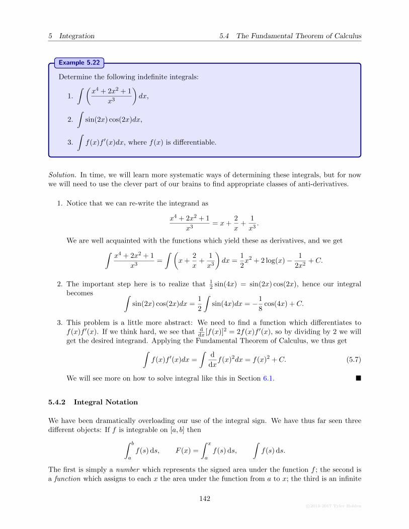
5 Integration 5.4 The Fundamental Theorem of Calculus
Example 5.22
Determine the following indefinite integrals:
1.
∫ (x4 + 2x2 + 1
x3
)dx,
2.
∫sin(2x) cos(2x)dx,
3.
∫f(x)f ′(x)dx, where f(x) is differentiable.
Solution. In time, we will learn more systematic ways of determining these integrals, but for nowwe will need to use the clever part of our brains to find appropriate classes of anti-derivatives.
1. Notice that we can re-write the integrand as
x4 + 2x2 + 1
x3= x+
2
x+
1
x3.
We are well acquainted with the functions which yield these as derivatives, and we get
∫x4 + 2x2 + 1
x3=
∫ (x+
2
x+
1
x3
)dx =
1
2x2 + 2 log(x)− 1
2x2+ C.
2. The important step here is to realize that 12 sin(4x) = sin(2x) cos(2x), hence our integral
becomes ∫sin(2x) cos(2x)dx =
1
2
∫sin(4x)dx = −1
8cos(4x) + C.
3. This problem is a little more abstract: We need to find a function which differentiates tof(x)f ′(x). If we think hard, we see that d
dx [f(x)]2 = 2f(x)f ′(x), so by dividing by 2 we willget the desired integrand. Applying the Fundamental Theorem of Calculus, we thus get
∫f(x)f ′(x)dx =
∫d
dxf(x)2dx = f(x)2 + C. (5.7)
We will see more on how to solve integral like this in Section 6.1. �
5.4.2 Integral Notation
We have been dramatically overloading our use of the integral sign. We have thus far seen threedifferent objects: If f is integrable on [a, b] then
∫ b
af(s) ds, F (x) =
∫ x
af(s) ds,
∫f(s) ds.
The first is simply a number which represents the signed area under the function f ; the second isa function which assigns to each x the area under the function from a to x; the third is an infinite
142c©2013-2017 Tyler Holden
6 Integration Techniques
family of functions, all representing anti-derivatives of f . They are all intimately related to becertain, but each has a very different lifestyle. One must be careful not to confuse the relationships.
Additionally, some authors prefer to the use the notation
∫dsf(s) instead of
∫f(s) ds.
There are occasions when this is useful, but we will never use it in this course.
6 Integration Techniques
In the following sections, we will develop a plethora of tools to help us compute integrals.
6.1 Integration by Substitution
Having seen that integration and differentiation are essentially inverses, we would like to developsome techniques and rules form computing integrals. It should be unsurprising that those ruleswill arise as the “inverse” operations of the rules obtained from differential calculus. We recall thechain rule of differential calculus tells us that
d
dxf(g(x)) = f ′(g(x))g′(x)
hence by applying the fundamental theorem of calculus, we see that
∫f ′(g(x))g′(x) dx = f(g(x)) + C. (6.1)
Unfortunately, the majority of times nature will conspire against us and not write our integrandso plainly as f ′(g(x))g′(x). Hence we develop some techniques to make life simpler. Our strategyis as follows:
1. Look to see if we can find the occurrence of a function and its derivative. In (6.1) above, weare looking for the function g(x), since it occurs in the argument of f(x) and its derivativeappears as g′(x).
2. Define a new variable, u = g(x) so that dudx = g′(x). We often write this second equation as
du = g′(x) dx.
3. Replace all x dependencies with u dependencies. Namely, recognize that
f ′(g(x))︸ ︷︷ ︸f(u)
g′(x) dx︸ ︷︷ ︸du
= f ′(u) du
4. Using the fundamental theorem of calculus, evaluate our new integral:
∫f ′(u) du = f(u) + C.
c©2013-2017 Tyler Holden
143
6 Integration Techniques 6.1 Integration by Substitution
5. We now have our solution, but it is in terms of the variable u. This is not a problem sincewe know that u = g(x), so we just make this substitution to get our final solution
∫f ′(g(x))g′(x) dx = f(g(x)) + C.
Let’s try a simple example:
Example 6.1
Determine
∫sin(2x) cos(2x) dx.
Solution. We can choose either u = sin(2x) or u = cos(2x). If u = sin(2x) then du = 2 cos(2x) dxand our integral becomes
∫sin(2x) cos(2x) dx =
1
2
∫udu =
1
4u2 + C =
1
2sin2(2x) + C.
On the other hand, if we choose u = cos(2x) then du = −12 sin(2x) and we get
∫sin(2x) cos(2x) dx = −1
2
∫udu = −1
4cos2(2x) + C.
Of course, we know that sin2(2x) and cos2(2x) are very different functions, and here we see theimportance of the constants.
To add to this bit of noise, notice that in Example 5.22 we calculated∫
sin(x) cos(x) =−1
8 cos(4x) + C. �
Example 6.2
For a, b 6= 0, compute
∫xn−1
√a+ bxn
dx.
Solution. Following the above program, our first step should be to identify a function and itsderivative. The fact that there is an xn and an xn−1 is a pretty good sign. Since constants donot affect the integration, we can make our lives even easier if we define u = a + bxn so thatdu = bnxn−1 dx. Unfortunately, there is no bnxn−1 dx in the integrand, but there is an xn−1 dx.Since these are related only up to a constant, we can divide both sides to find that xn−1 dx = 1
bn du.Adding our substitutions we then get
∫xn−1
√a+ bxn
dx =
∫ 1bn du√u
=1
bn
∫1√u
du.
This is now a very simple integral to calculate, and indeed we find that
1
bn
∫1√u
du =2
bn
√u+ C.
144c©2013-2017 Tyler Holden
6.1 Integration by Substitution 6 Integration Techniques
We need this to be in terms of x rather than u, so we recall that u = a+ bxn to finally find that∫
xn−1
√a+ bxn
dx =2
bn
√a+ bxn + C. �
Substitution is not just handy for applying the chain rule. It also allows us to “change variables.”
Example 6.3
Compute
∫x√x+ 1 dx.
Solution. Notice that if we could somehow switch the x and the x+ 1, this integral would be muchsimpler, since then (x+ 1)
√x = x3/2 +x. Normally in mathematics, if we want to do such a thing,
we just define a new variable u = x+ 1 so that x = u− 1 and then a similar trick to the one abovewill work.
Since we are working with an integral though, we must be a bit more careful. We shall stilldefine u = x + 1 with x = u − 1, but we must also track the differentials. Luckily, in this casedu = dx and there is nothing to do. We thus get
∫x√x+ 1 dx =
∫(u− 1)
√udu
=
∫(u3/2 −√u) du
=2
5u5/2 − 2
3u3/2 + C.
Converting back to a function of x yields∫x√x+ 1 dx =
2
5(x+ 1)5/2 − 1
2(x+ 1)2 + C. �
6.1.1 Definite Integrals
When dealing with definite integrals, we adhere to the same process as indefinite integrals, but wemust also accommodate the lower and upper bounds of integration. Let f be a continuous functionwith anti-derivative F , while g is continuously differentiable. Once again consider the case whenwe are integrating the function ∫ b
af(g(x))g′(x) dx.
We know that F (g(x)) is an integrable anti-derivative, so the Fundamental Theorem of Calculusimplies that ∫ b
af(g(x))g′(x) dx = [F (g(x))]ba = F (g(b))− F (g(a)).
This implies that the correct lower and upper bounds of integration are g(a) and g(b) respectively,since ∫ b
af(g(x))g′(x) dx =
∫ g(b)
g(a)f(u) du = [F (u)]
g(b)g(a) = F (g(b))− F (g(a))
c©2013-2017 Tyler Holden
145
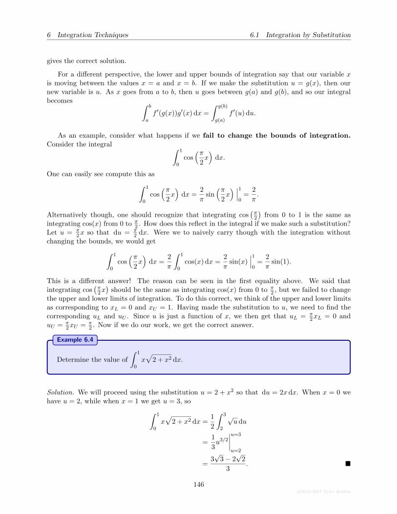
6 Integration Techniques 6.1 Integration by Substitution
gives the correct solution.
For a different perspective, the lower and upper bounds of integration say that our variable xis moving between the values x = a and x = b. If we make the substitution u = g(x), then ournew variable is u. As x goes from a to b, then u goes between g(a) and g(b), and so our integralbecomes ∫ b
af ′(g(x))g′(x) dx =
∫ g(b)
g(a)f ′(u) du.
As an example, consider what happens if we fail to change the bounds of integration.Consider the integral ∫ 1
0cos(π
2x)
dx.
One can easily see compute this as
∫ 1
0cos(π
2x)
dx =2
πsin(π
2x) ∣∣∣
1
0=
2
π.
Alternatively though, one should recognize that integrating cos(π2
)from 0 to 1 is the same as
integrating cos(x) from 0 to π2 . How does this reflect in the integral if we make such a substitution?
Let u = π2x so that du = π
2 dx. Were we to naively carry though with the integration withoutchanging the bounds, we would get
∫ 1
0cos(π
2x)
dx =2
π
∫ 1
0cos(x) dx =
2
πsin(x)
∣∣∣1
0=
2
πsin(1).
This is a different answer! The reason can be seen in the first equality above. We said thatintegrating cos
(π2x)
should be the same as integrating cos(x) from 0 to π2 , but we failed to change
the upper and lower limits of integration. To do this correct, we think of the upper and lower limitsas corresponding to xL = 0 and xU = 1. Having made the substitution to u, we need to find thecorresponding uL and uU . Since u is just a function of x, we then get that uL = π
2xL = 0 anduU = π
2xU = π2 . Now if we do our work, we get the correct answer.
Example 6.4
Determine the value of
∫ 1
0x√
2 + x2 dx.
Solution. We will proceed using the substitution u = 2 + x2 so that du = 2x dx. When x = 0 wehave u = 2, while when x = 1 we get u = 3, so
∫ 1
0x√
2 + x2 dx =1
2
∫ 3
2
√udu
=1
3u3/2
∣∣∣∣u=3
u=2
=3√
3− 2√
2
3. �
146c©2013-2017 Tyler Holden
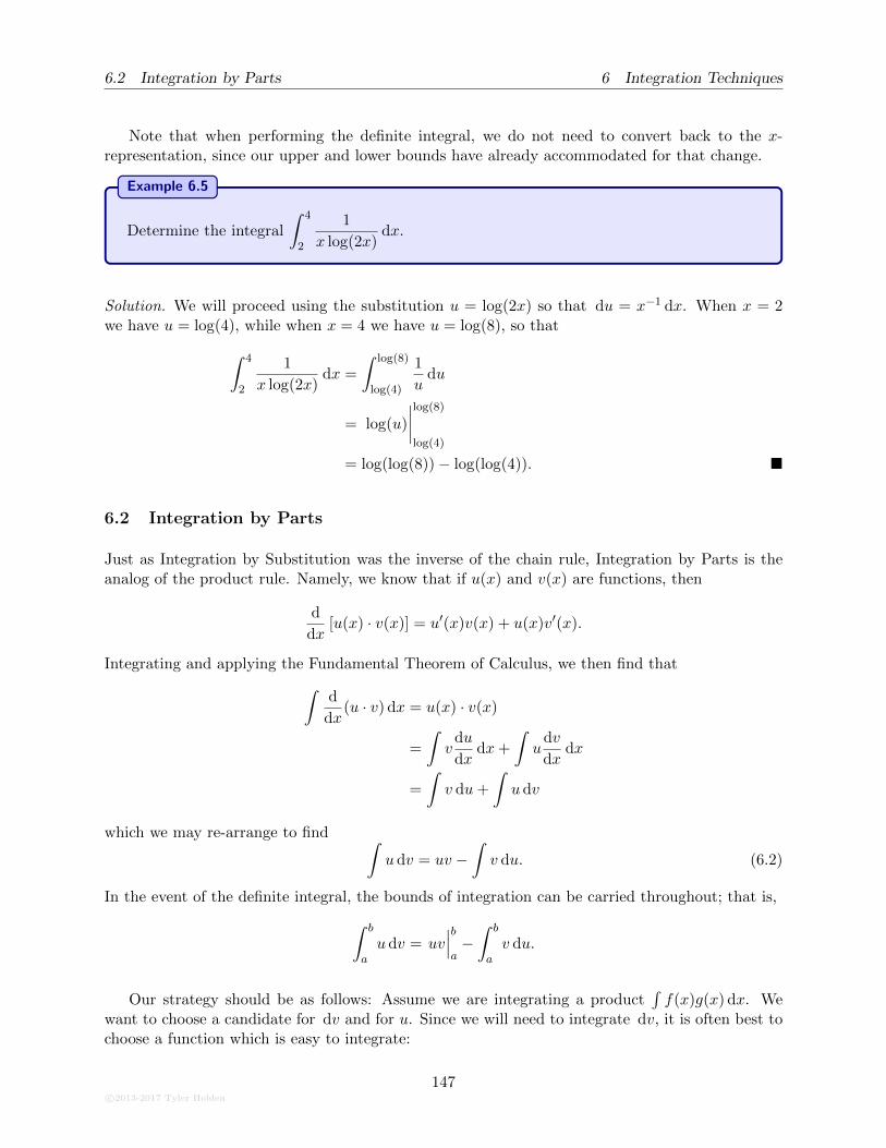
6.2 Integration by Parts 6 Integration Techniques
Note that when performing the definite integral, we do not need to convert back to the x-representation, since our upper and lower bounds have already accommodated for that change.
Example 6.5
Determine the integral
∫ 4
2
1
x log(2x)dx.
Solution. We will proceed using the substitution u = log(2x) so that du = x−1 dx. When x = 2we have u = log(4), while when x = 4 we have u = log(8), so that
∫ 4
2
1
x log(2x)dx =
∫ log(8)
log(4)
1
udu
= log(u)
∣∣∣∣log(8)
log(4)
= log(log(8))− log(log(4)). �
6.2 Integration by Parts
Just as Integration by Substitution was the inverse of the chain rule, Integration by Parts is theanalog of the product rule. Namely, we know that if u(x) and v(x) are functions, then
d
dx[u(x) · v(x)] = u′(x)v(x) + u(x)v′(x).
Integrating and applying the Fundamental Theorem of Calculus, we then find that
∫d
dx(u · v) dx = u(x) · v(x)
=
∫v
du
dxdx+
∫u
dv
dxdx
=
∫v du+
∫udv
which we may re-arrange to find ∫u dv = uv −
∫v du. (6.2)
In the event of the definite integral, the bounds of integration can be carried throughout; that is,
∫ b
audv = uv
∣∣∣b
a−∫ b
av du.
Our strategy should be as follows: Assume we are integrating a product∫f(x)g(x) dx. We
want to choose a candidate for dv and for u. Since we will need to integrate dv, it is often best tochoose a function which is easy to integrate:
c©2013-2017 Tyler Holden
147
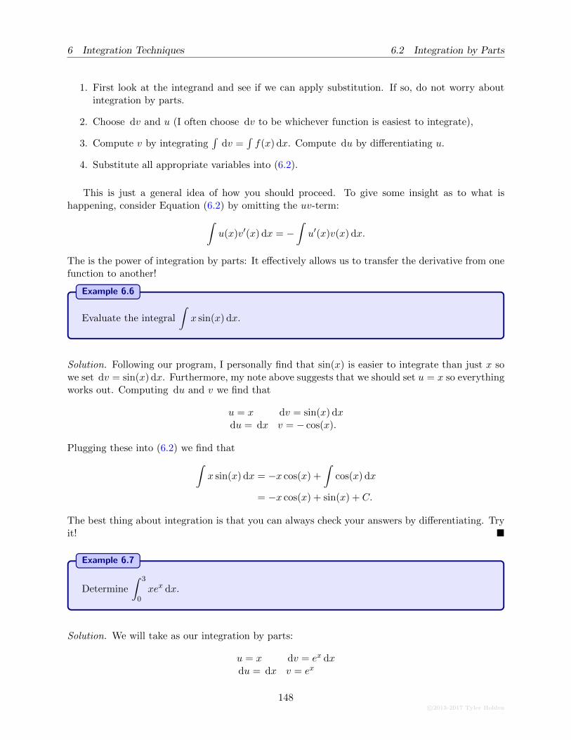
6 Integration Techniques 6.2 Integration by Parts
1. First look at the integrand and see if we can apply substitution. If so, do not worry aboutintegration by parts.
2. Choose dv and u (I often choose dv to be whichever function is easiest to integrate),
3. Compute v by integrating∫
dv =∫f(x) dx. Compute du by differentiating u.
4. Substitute all appropriate variables into (6.2).
This is just a general idea of how you should proceed. To give some insight as to what ishappening, consider Equation (6.2) by omitting the uv-term:
∫u(x)v′(x) dx = −
∫u′(x)v(x) dx.
The is the power of integration by parts: It effectively allows us to transfer the derivative from onefunction to another!
Example 6.6
Evaluate the integral
∫x sin(x) dx.
Solution. Following our program, I personally find that sin(x) is easier to integrate than just x sowe set dv = sin(x) dx. Furthermore, my note above suggests that we should set u = x so everythingworks out. Computing du and v we find that
u = x dv = sin(x) dxdu = dx v = − cos(x).
Plugging these into (6.2) we find that
∫x sin(x) dx = −x cos(x) +
∫cos(x) dx
= −x cos(x) + sin(x) + C.
The best thing about integration is that you can always check your answers by differentiating. Tryit! �
Example 6.7
Determine
∫ 3
0xex dx.
Solution. We will take as our integration by parts:
u = x dv = ex dxdu = dx v = ex
148c©2013-2017 Tyler Holden
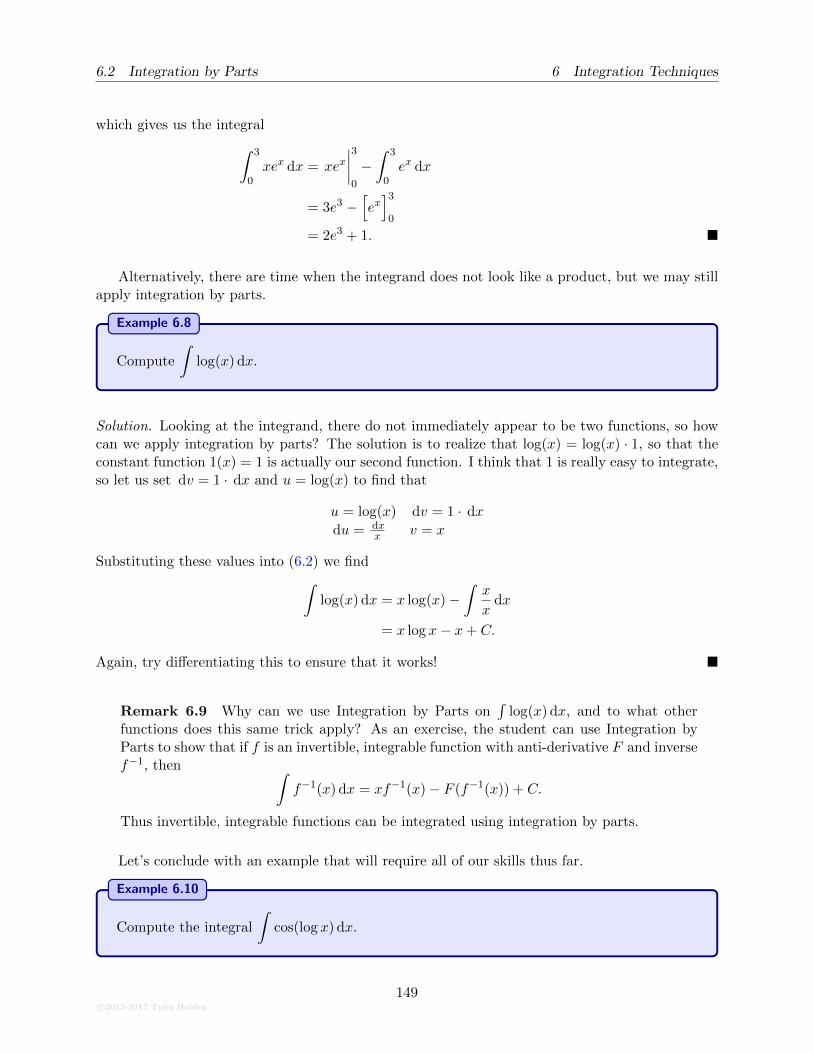
6.2 Integration by Parts 6 Integration Techniques
which gives us the integral
∫ 3
0xex dx = xex
∣∣∣∣3
0
−∫ 3
0ex dx
= 3e3 −[ex]3
0
= 2e3 + 1. �
Alternatively, there are time when the integrand does not look like a product, but we may stillapply integration by parts.
Example 6.8
Compute
∫log(x) dx.
Solution. Looking at the integrand, there do not immediately appear to be two functions, so howcan we apply integration by parts? The solution is to realize that log(x) = log(x) · 1, so that theconstant function 1(x) = 1 is actually our second function. I think that 1 is really easy to integrate,so let us set dv = 1 · dx and u = log(x) to find that
u = log(x) dv = 1 · dx
du = dxx v = x
Substituting these values into (6.2) we find
∫log(x) dx = x log(x)−
∫x
xdx
= x log x− x+ C.
Again, try differentiating this to ensure that it works! �
Remark 6.9 Why can we use Integration by Parts on∫
log(x) dx, and to what otherfunctions does this same trick apply? As an exercise, the student can use Integration byParts to show that if f is an invertible, integrable function with anti-derivative F and inversef−1, then ∫
f−1(x) dx = xf−1(x)− F (f−1(x)) + C.
Thus invertible, integrable functions can be integrated using integration by parts.
Let’s conclude with an example that will require all of our skills thus far.
Example 6.10
Compute the integral
∫cos(log x) dx.
c©2013-2017 Tyler Holden
149
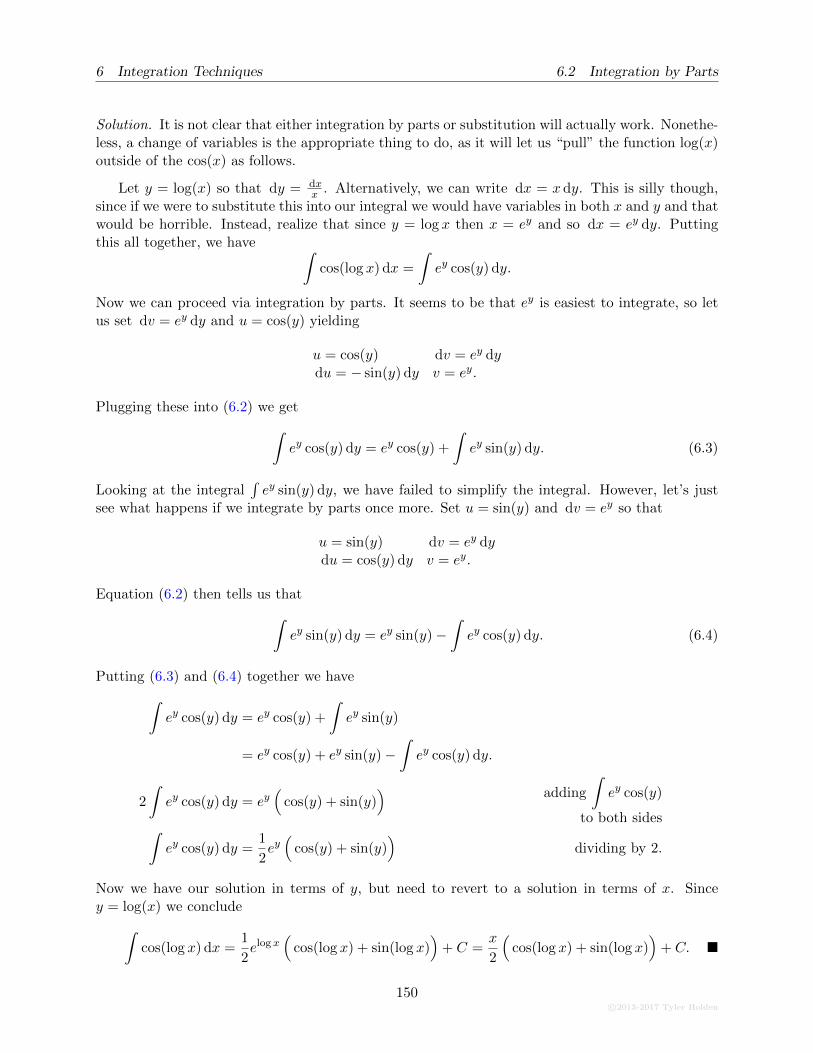
6 Integration Techniques 6.2 Integration by Parts
Solution. It is not clear that either integration by parts or substitution will actually work. Nonethe-less, a change of variables is the appropriate thing to do, as it will let us “pull” the function log(x)outside of the cos(x) as follows.
Let y = log(x) so that dy = dxx . Alternatively, we can write dx = x dy. This is silly though,
since if we were to substitute this into our integral we would have variables in both x and y and thatwould be horrible. Instead, realize that since y = log x then x = ey and so dx = ey dy. Puttingthis all together, we have ∫
cos(log x) dx =
∫ey cos(y) dy.
Now we can proceed via integration by parts. It seems to be that ey is easiest to integrate, so letus set dv = ey dy and u = cos(y) yielding
u = cos(y) dv = ey dydu = − sin(y) dy v = ey.
Plugging these into (6.2) we get
∫ey cos(y) dy = ey cos(y) +
∫ey sin(y) dy. (6.3)
Looking at the integral∫ey sin(y) dy, we have failed to simplify the integral. However, let’s just
see what happens if we integrate by parts once more. Set u = sin(y) and dv = ey so that
u = sin(y) dv = ey dydu = cos(y) dy v = ey.
Equation (6.2) then tells us that
∫ey sin(y) dy = ey sin(y)−
∫ey cos(y) dy. (6.4)
Putting (6.3) and (6.4) together we have
∫ey cos(y) dy = ey cos(y) +
∫ey sin(y)
= ey cos(y) + ey sin(y)−∫ey cos(y) dy.
2
∫ey cos(y) dy = ey
(cos(y) + sin(y)
) adding
∫ey cos(y)
to both sides∫ey cos(y) dy =
1
2ey(
cos(y) + sin(y))
dividing by 2.
Now we have our solution in terms of y, but need to revert to a solution in terms of x. Sincey = log(x) we conclude
∫cos(log x) dx =
1
2elog x
(cos(log x) + sin(log x)
)+ C =
x
2
(cos(log x) + sin(log x)
)+ C. �
150c©2013-2017 Tyler Holden
6.3 Integrating Trigonometric Functions 6 Integration Techniques
6.3 Integrating Trigonometric Functions
Integrating trigonometric functions often comes down to a combination of using the Pythagoreanidentities, or angle sum identities. Notice very conveniently that the three Pythagorean identitiesare
• sin2(x) + cos2(x) = 1, and ddx sin(x) = cos(x), d
dx cos(x) = − sin(x),
• tan2(x) + 1 = sec2(x), and ddx tan(x) = sec2(x), d
dx sec(x) = sec(x) tan(x)
• 1 + cot2(x) = csc2(x), and ddx cot(x) = − csc2(x), d
dx csc(x) = − csc(x) cot(x).
Hence each identity only contains the components of a function and its derivatives. This will proveto be an exceptionally useful tool shortly.
The other trick to remember is the following two identities:
sin2(x) =1
2(1− cos(2x)), and cos2(x) =
1
2(1 + cos(2x)).
We can immediately use the above to equations to see that
∫sin2(x) dx =
∫1
2[1− cos(2x)] dx
=1
2x− 1
4sin(2x) + C.
∫cos2(x) dx =
1
2
∫[1 + cos(2x)] dx
=1
2x+
1
4sin(2x) + C.
Now what happens if our integrand is made up a several different trigonometric functions? Forexample, how would we deal with something of the form
∫sin2(x) cos3(x) dx?
The idea is to use the Pythagorean identities listed above to reduce the integrand to an expressionof the form g(f(x))f ′(x) dx, since from here one can easily apply the substitution method: indeed,
∫g(f(x))f ′(x) dx =
∫g(u) du
u = f(x)du = f ′(x) dx
= G(f(x)) + C
for some anti-derivative G of g.
Returning to our example,∫
sin2(x) cos3(x) dx, we see that by writing
cos3(x) = cos2(x) cos(x) = (1− sin2(x)) cos(x)
c©2013-2017 Tyler Holden
151
6 Integration Techniques 6.3 Integrating Trigonometric Functions
our integral becomes∫
sin2(x) cos3(x) dx =
∫sin2(x)(1− sin2(x)) cos(x) dx.
Our integrand now consists entire of sine functions, and a single cosine function which will serveas a substitution. Setting u = sin(x) so that du = cos(x) dx we have
∫sin2(x) cos3(x) dx =
∫sin2(x)[1− sin2(x)] cos(x) dx
=
∫u2(1− u2) du
=1
3u3 − 1
5u5 + C
=1
3sin3(x)− 1
5sin5(x) + C.
Example 6.11
Determine the integral
∫sec4(x) tan5(x) dx.
Solution. One again we conveniently have only secant and tangent functions, which are intimatelyrelated to one another through their derivatives. We have to now determine which function we aregoing to use as a substitution. If we make the substitution u = tan(x) then du = sec2(x) dx andour integral becomes
∫sec4(x) tan5(x) dx =
∫sec3(x) tan4(x) du =
∫sec3(x)u4 du.
But now we are in trouble, since there is no obvious way to turn sec3(x) into a function involvingonly tan(x).
Let’s try the other substitution. If we make the u = sec(x) substitution, we will have du =sec(x) tan(x) and so our integral will become
∫sec4(x) tan5(x) dx =
∫sec3(x) tan4(x) du =
∫tan4(x)u3 du.
This is perfect, since tan4(x) = [tan2(x)]2 = [sec2(x)− 1]2. Hence we can compute our integral as∫
sec4(x) tan5(x) dx =
∫ [u2 − 1
]2u3 du
=1
8u8 − 1
3u6 +
1
4u4 + C
=1
8sec8(x)− 1
3sec6(x) +
1
4sec4(x) + C. �
The previous two example really seem to indicate the importance that the powers of one of thefunctions have odd degree. In the event that everything is of even degree, we once again have touse our identities on relating sin2(x) and cos2(x) to cos(2x).
152c©2013-2017 Tyler Holden
6.3 Integrating Trigonometric Functions 6 Integration Techniques
Example 6.12
Determine the integral
∫cos4(x) dx.
Solution. We know that cos2(x) = 12(1 + cos(2x)) and so our integral becomes
∫cos4(x) dx =
1
4
∫[1 + cos(2x)] [1 + cos(2x)] dx
=1
4
∫ [1 + 2 cos(2x) + cos2(2x)
]dx
=1
4[x+ sin(2x)] +
1
4
∫cos2(2x) dx
=1
4x+
1
4sin(2x) +
1
8
∫[1 + cos(4x)] dx
=3
8x+
1
4sin(2x) +
1
32sin(4x) + C. �
Example 6.13
Determine the integral
∫ π/2
0sin3(x) dx.
Solution. We have three sines, so we will keep one and turn to the other two into cosines.
sin3(x) = sin(x) sin2(x) = sin(x)[1− cos2(x)
].
Our integral is thus
∫ π/2
0sin3(x) dx =
∫ π/2
0sin(x)
[1− cos2(x)
]dx
= −∫ 0
1(1− u2) du
u = cos(x)du = − sin(x) dx
=
[u− 1
3u3
]1
0
=2
3. �
One could enumerate a rather large list of all the possible cases and the tricks to use, but this isa rather large waste of time. Instead, the student should just realize that the fundamental idea isto apply trigonometric identities in a way that isolates a single occurrence of a function’s derivativeand then apply substitution.
c©2013-2017 Tyler Holden
153
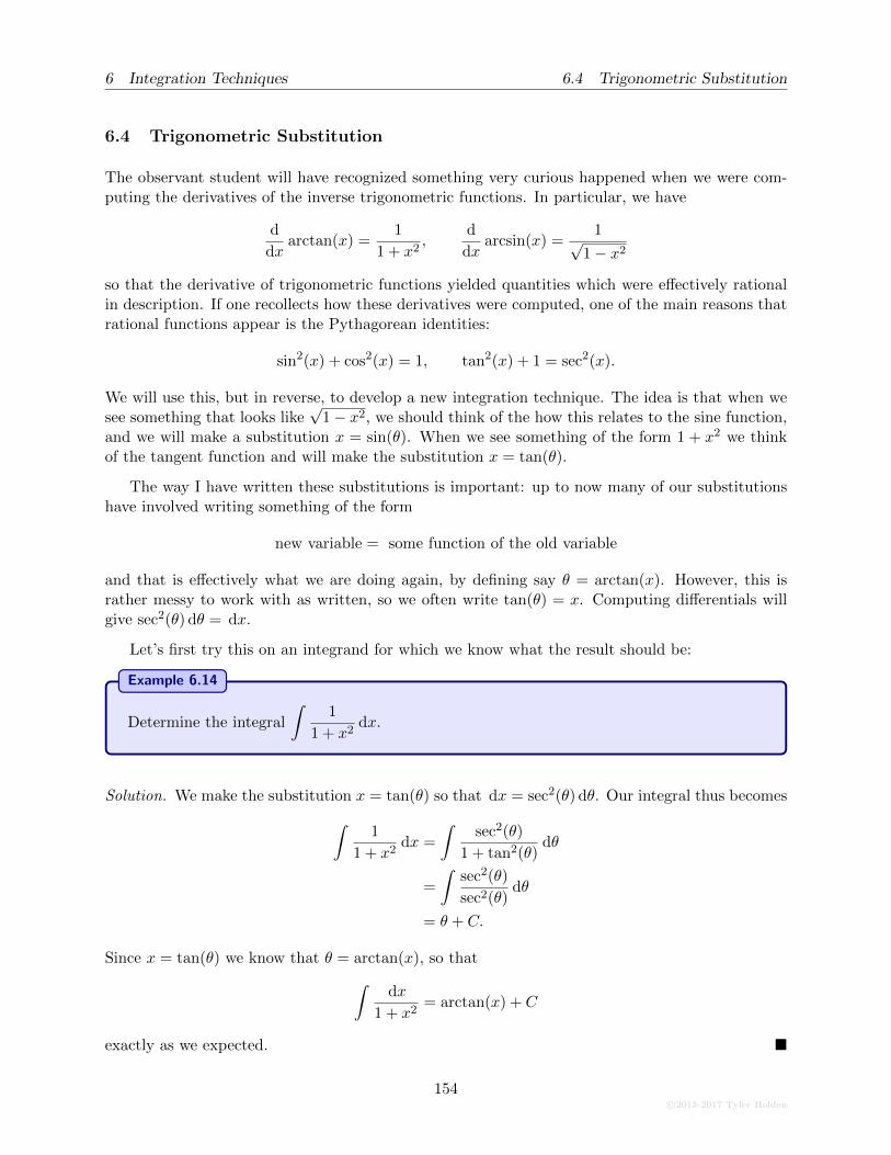
6 Integration Techniques 6.4 Trigonometric Substitution
6.4 Trigonometric Substitution
The observant student will have recognized something very curious happened when we were com-puting the derivatives of the inverse trigonometric functions. In particular, we have
d
dxarctan(x) =
1
1 + x2,
d
dxarcsin(x) =
1√1− x2
so that the derivative of trigonometric functions yielded quantities which were effectively rationalin description. If one recollects how these derivatives were computed, one of the main reasons thatrational functions appear is the Pythagorean identities:
sin2(x) + cos2(x) = 1, tan2(x) + 1 = sec2(x).
We will use this, but in reverse, to develop a new integration technique. The idea is that when wesee something that looks like
√1− x2, we should think of the how this relates to the sine function,
and we will make a substitution x = sin(θ). When we see something of the form 1 + x2 we thinkof the tangent function and will make the substitution x = tan(θ).
The way I have written these substitutions is important: up to now many of our substitutionshave involved writing something of the form
new variable = some function of the old variable
and that is effectively what we are doing again, by defining say θ = arctan(x). However, this israther messy to work with as written, so we often write tan(θ) = x. Computing differentials willgive sec2(θ) dθ = dx.
Let’s first try this on an integrand for which we know what the result should be:
Example 6.14
Determine the integral
∫1
1 + x2dx.
Solution. We make the substitution x = tan(θ) so that dx = sec2(θ) dθ. Our integral thus becomes
∫1
1 + x2dx =
∫sec2(θ)
1 + tan2(θ)dθ
=
∫sec2(θ)
sec2(θ)dθ
= θ + C.
Since x = tan(θ) we know that θ = arctan(x), so that
∫dx
1 + x2= arctan(x) + C
exactly as we expected. �
154c©2013-2017 Tyler Holden
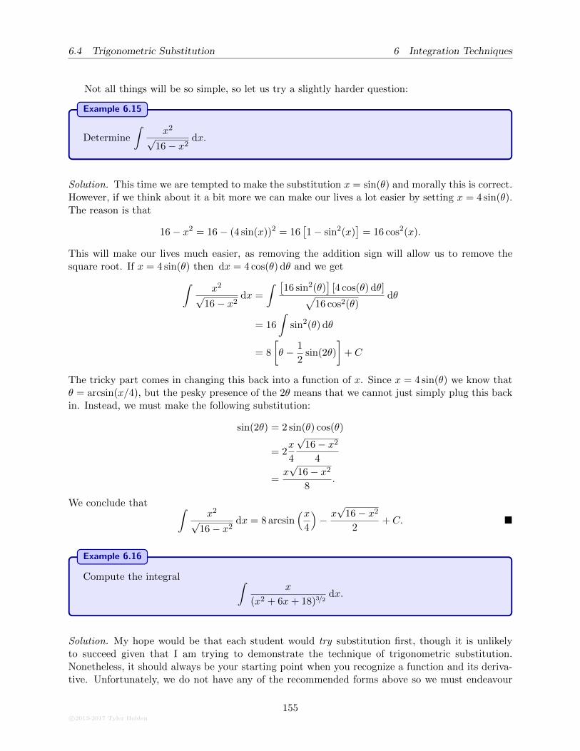
6.4 Trigonometric Substitution 6 Integration Techniques
Not all things will be so simple, so let us try a slightly harder question:
Example 6.15
Determine
∫x2
√16− x2
dx.
Solution. This time we are tempted to make the substitution x = sin(θ) and morally this is correct.However, if we think about it a bit more we can make our lives a lot easier by setting x = 4 sin(θ).The reason is that
16− x2 = 16− (4 sin(x))2 = 16[1− sin2(x)
]= 16 cos2(x).
This will make our lives much easier, as removing the addition sign will allow us to remove thesquare root. If x = 4 sin(θ) then dx = 4 cos(θ) dθ and we get
∫x2
√16− x2
dx =
∫ [16 sin2(θ)
][4 cos(θ) dθ]√
16 cos2(θ)dθ
= 16
∫sin2(θ) dθ
= 8
[θ − 1
2sin(2θ)
]+ C
The tricky part comes in changing this back into a function of x. Since x = 4 sin(θ) we know thatθ = arcsin(x/4), but the pesky presence of the 2θ means that we cannot just simply plug this backin. Instead, we must make the following substitution:
sin(2θ) = 2 sin(θ) cos(θ)
= 2x
4
√16− x2
4
=x√
16− x2
8.
We conclude that ∫x2
√16− x2
dx = 8 arcsin(x
4
)− x√
16− x2
2+ C. �
Example 6.16
Compute the integral ∫x
(x2 + 6x+ 18)3/2dx.
Solution. My hope would be that each student would try substitution first, though it is unlikelyto succeed given that I am trying to demonstrate the technique of trigonometric substitution.Nonetheless, it should always be your starting point when you recognize a function and its deriva-tive. Unfortunately, we do not have any of the recommended forms above so we must endeavour
c©2013-2017 Tyler Holden
155
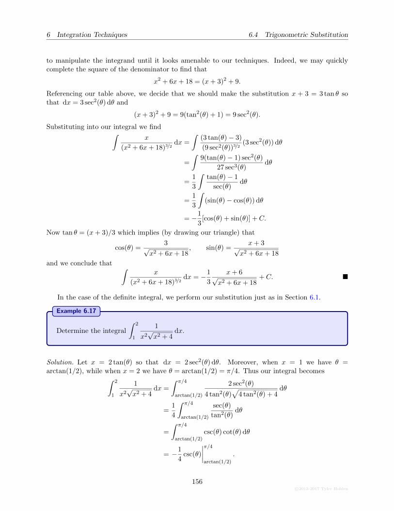
6 Integration Techniques 6.4 Trigonometric Substitution
to manipulate the integrand until it looks amenable to our techniques. Indeed, we may quicklycomplete the square of the denominator to find that
x2 + 6x+ 18 = (x+ 3)2 + 9.
Referencing our table above, we decide that we should make the substitution x + 3 = 3 tan θ sothat dx = 3 sec2(θ) dθ and
(x+ 3)2 + 9 = 9(tan2(θ) + 1) = 9 sec2(θ).
Substituting into our integral we find∫
x
(x2 + 6x+ 18)3/2dx =
∫(3 tan(θ)− 3)
(9 sec2(θ))3/2(3 sec2(θ)) dθ
=
∫9(tan(θ)− 1) sec2(θ)
27 sec3(θ)dθ
=1
3
∫tan(θ)− 1
sec(θ)dθ
=1
3
∫(sin(θ)− cos(θ)) dθ
= −1
3[cos(θ) + sin(θ)] + C.
Now tan θ = (x+ 3)/3 which implies (by drawing our triangle) that
cos(θ) =3√
x2 + 6x+ 18, sin(θ) =
x+ 3√x2 + 6x+ 18
and we conclude that ∫x
(x2 + 6x+ 18)3/2dx = −1
3
x+ 6√x2 + 6x+ 18
+ C. �
In the case of the definite integral, we perform our substitution just as in Section 6.1.
Example 6.17
Determine the integral
∫ 2
1
1
x2√x2 + 4
dx.
Solution. Let x = 2 tan(θ) so that dx = 2 sec2(θ) dθ. Moreover, when x = 1 we have θ =arctan(1/2), while when x = 2 we have θ = arctan(1/2) = π/4. Thus our integral becomes
∫ 2
1
1
x2√x2 + 4
dx =
∫ π/4
arctan(1/2)
2 sec2(θ)
4 tan2(θ)√
4 tan2(θ) + 4dθ
=1
4
∫ π/4
arctan(1/2)
sec(θ)
tan2(θ)dθ
=
∫ π/4
arctan(1/2)csc(θ) cot(θ) dθ
= −1
4csc(θ)
∣∣∣∣π/4
arctan(1/2)
.
156c©2013-2017 Tyler Holden
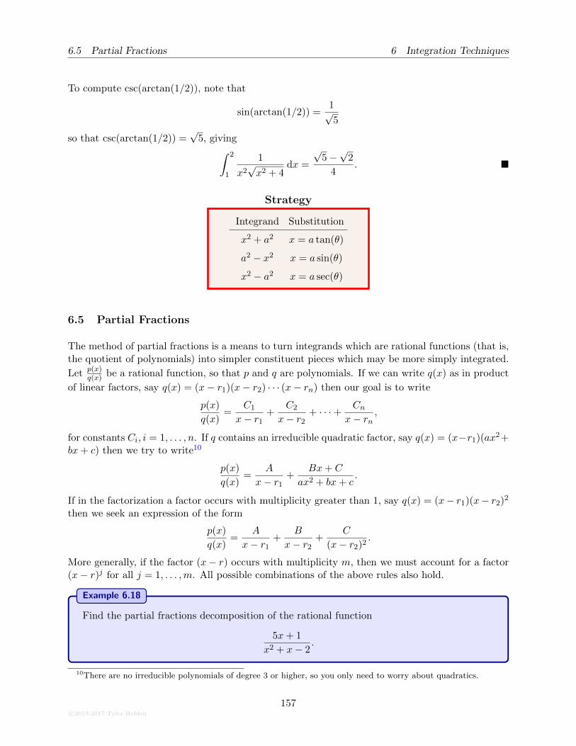
6.5 Partial Fractions 6 Integration Techniques
To compute csc(arctan(1/2)), note that
sin(arctan(1/2)) =1√5
so that csc(arctan(1/2)) =√
5, giving∫ 2
1
1
x2√x2 + 4
dx =
√5−√
2
4. �
Strategy
Integrand Substitution
x2 + a2 x = a tan(θ)
a2 − x2 x = a sin(θ)
x2 − a2 x = a sec(θ)
6.5 Partial Fractions
The method of partial fractions is a means to turn integrands which are rational functions (that is,the quotient of polynomials) into simpler constituent pieces which may be more simply integrated.
Let p(x)q(x) be a rational function, so that p and q are polynomials. If we can write q(x) as in product
of linear factors, say q(x) = (x− r1)(x− r2) · · · (x− rn) then our goal is to write
p(x)
q(x)=
C1
x− r1+
C2
x− r2+ · · ·+ Cn
x− rn,
for constants Ci, i = 1, . . . , n. If q contains an irreducible quadratic factor, say q(x) = (x−r1)(ax2+bx+ c) then we try to write10
p(x)
q(x)=
A
x− r1+
Bx+ C
ax2 + bx+ c.
If in the factorization a factor occurs with multiplicity greater than 1, say q(x) = (x− r1)(x− r2)2
then we seek an expression of the form
p(x)
q(x)=
A
x− r1+
B
x− r2+
C
(x− r2)2.
More generally, if the factor (x− r) occurs with multiplicity m, then we must account for a factor(x− r)j for all j = 1, . . . ,m. All possible combinations of the above rules also hold.
Example 6.18
Find the partial fractions decomposition of the rational function
5x+ 1
x2 + x− 2.
10There are no irreducible polynomials of degree 3 or higher, so you only need to worry about quadratics.
c©2013-2017 Tyler Holden
157
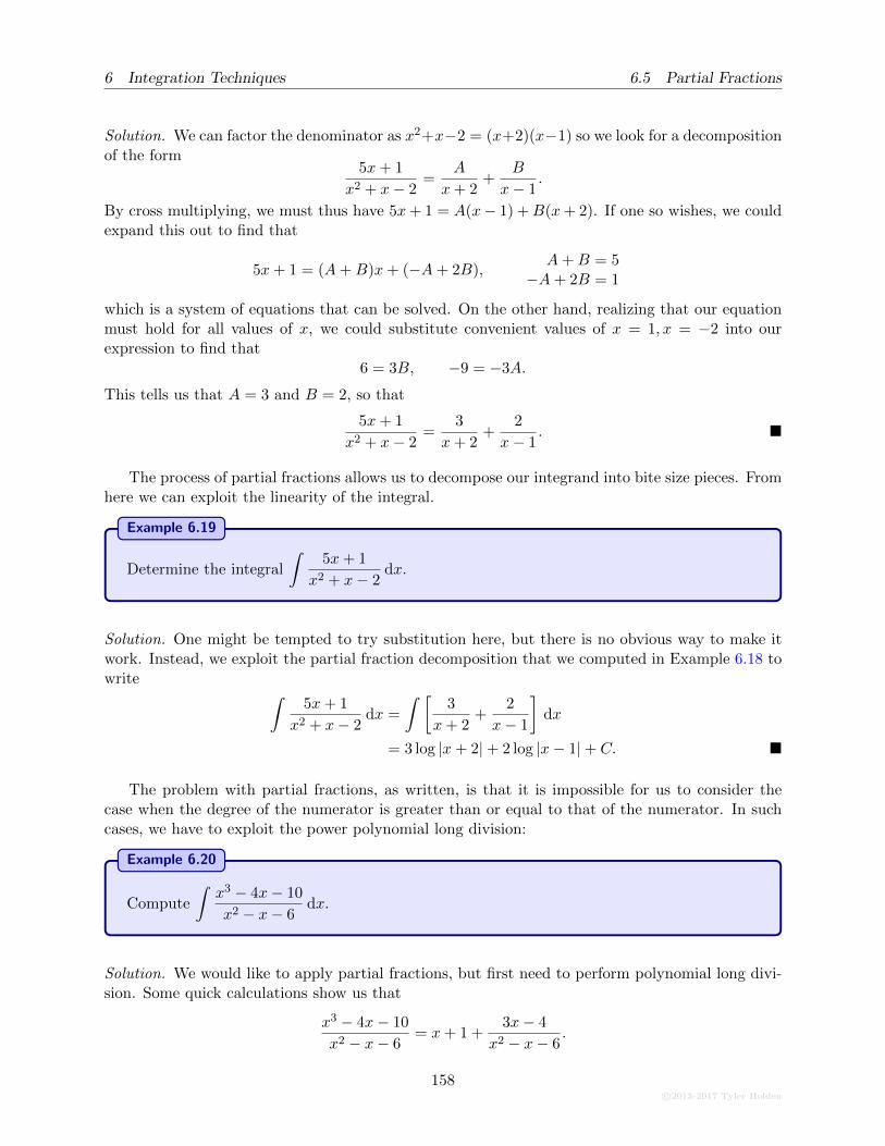
6 Integration Techniques 6.5 Partial Fractions
Solution. We can factor the denominator as x2+x−2 = (x+2)(x−1) so we look for a decompositionof the form
5x+ 1
x2 + x− 2=
A
x+ 2+
B
x− 1.
By cross multiplying, we must thus have 5x+ 1 = A(x− 1) +B(x+ 2). If one so wishes, we couldexpand this out to find that
5x+ 1 = (A+B)x+ (−A+ 2B),A+B = 5
−A+ 2B = 1
which is a system of equations that can be solved. On the other hand, realizing that our equationmust hold for all values of x, we could substitute convenient values of x = 1, x = −2 into ourexpression to find that
6 = 3B, −9 = −3A.
This tells us that A = 3 and B = 2, so that
5x+ 1
x2 + x− 2=
3
x+ 2+
2
x− 1. �
The process of partial fractions allows us to decompose our integrand into bite size pieces. Fromhere we can exploit the linearity of the integral.
Example 6.19
Determine the integral
∫5x+ 1
x2 + x− 2dx.
Solution. One might be tempted to try substitution here, but there is no obvious way to make itwork. Instead, we exploit the partial fraction decomposition that we computed in Example 6.18 towrite
∫5x+ 1
x2 + x− 2dx =
∫ [3
x+ 2+
2
x− 1
]dx
= 3 log |x+ 2|+ 2 log |x− 1|+ C. �
The problem with partial fractions, as written, is that it is impossible for us to consider thecase when the degree of the numerator is greater than or equal to that of the numerator. In suchcases, we have to exploit the power polynomial long division:
Example 6.20
Compute
∫x3 − 4x− 10
x2 − x− 6dx.
Solution. We would like to apply partial fractions, but first need to perform polynomial long divi-sion. Some quick calculations show us that
x3 − 4x− 10
x2 − x− 6= x+ 1 +
3x− 4
x2 − x− 6.
158c©2013-2017 Tyler Holden
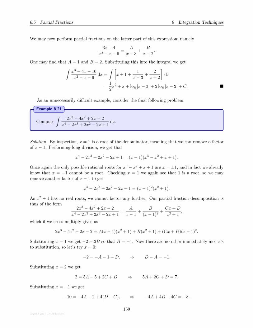
6.5 Partial Fractions 6 Integration Techniques
We may now perform partial fractions on the latter part of this expression; namely
3x− 4
x2 − x− 6=
A
x− 3+
B
x− 2.
One may find that A = 1 and B = 2. Substituting this into the integral we get
∫x3 − 4x− 10
x2 − x− 6dx =
∫ [x+ 1 +
1
x− 3+
2
x+ 2
]dx
=1
2x2 + x+ log |x− 3|+ 2 log |x− 2|+ C. �
As an unnecessarily difficult example, consider the final following problem:
Example 6.21
Compute
∫2x3 − 4x2 + 2x− 2
x4 − 2x3 + 2x2 − 2x+ 1dx.
Solution. By inspection, x = 1 is a root of the denominator, meaning that we can remove a factorof x− 1. Performing long division, we get that
x4 − 2x3 + 2x2 − 2x+ 1 = (x− 1)(x3 − x2 + x+ 1).
Once again the only possible rational roots for x3 − x2 + x+ 1 are x = ±1, and in fact we alreadyknow that x = −1 cannot be a root. Checking x = 1 we again see that 1 is a root, so we mayremove another factor of x− 1 to get
x4 − 2x3 + 2x2 − 2x+ 1 = (x− 1)2(x2 + 1).
As x2 + 1 has no real roots, we cannot factor any further. Our partial fraction decomposition isthus of the form
2x3 − 4x2 + 2x− 2
x4 − 2x3 + 2x2 − 2x+ 1=
A
x− 1+
B
(x− 1)2+Cx+D
x2 + 1,
which if we cross multiply gives us
2x3 − 4x2 + 2x− 2 = A(x− 1)(x2 + 1) +B(x2 + 1) + (Cx+D)(x− 1)2.
Substituting x = 1 we get −2 = 2B so that B = −1. Now there are no other immediately nice x’sto substitution, so let’s try x = 0:
−2 = −A− 1 +D, ⇒ D −A = −1.
Substituting x = 2 we get
2 = 5A− 5 + 2C +D ⇒ 5A+ 2C +D = 7.
Substituting x = −1 we get
−10 = −4A− 2 + 4(D − C), ⇒ −4A+ 4D − 4C = −8.
c©2013-2017 Tyler Holden
159
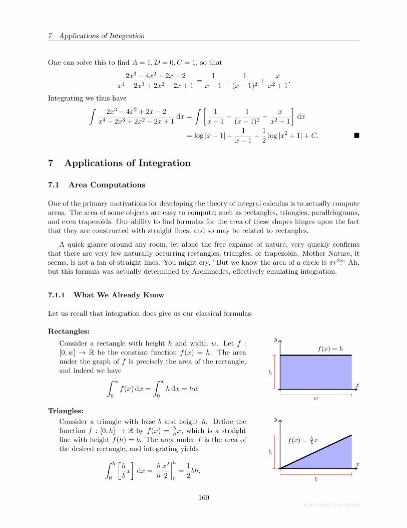
7 Applications of Integration
One can solve this to find A = 1, D = 0, C = 1, so that
2x3 − 4x2 + 2x− 2
x4 − 2x3 + 2x2 − 2x+ 1=
1
x− 1− 1
(x− 1)2+
x
x2 + 1.
Integrating we thus have∫
2x3 − 4x2 + 2x− 2
x4 − 2x3 + 2x2 − 2x+ 1dx =
∫ [1
x− 1− 1
(x− 1)2+
x
x2 + 1
]dx
= log |x− 1|+ 1
x− 1+
1
2log |x2 + 1|+ C. �
7 Applications of Integration
7.1 Area Computations
One of the primary motivations for developing the theory of integral calculus is to actually computeareas. The area of some objects are easy to compute; such as rectangles, triangles, parallelograms,and even trapezoids. Our ability to find formulas for the area of these shapes hinges upon the factthat they are constructed with straight lines, and so may be related to rectangles.
A quick glance around any room, let alone the free expanse of nature, very quickly confirmsthat there are very few naturally occurring rectangles, triangles, or trapezoids. Mother Nature, itseems, is not a fan of straight lines. You might cry, ”But we know the area of a circle is πr2!” Ah,but this formula was actually determined by Archimedes, effectively emulating integration.
7.1.1 What We Already Know
Let us recall that integration does give us our classical formulas:
Rectangles:
Consider a rectangle with height h and width w. Let f :[0, w] → R be the constant function f(x) = h. The areaunder the graph of f is precisely the area of the rectangle,and indeed we have
∫ w
0f(x) dx =
∫ w
0hdx = hw
x
y
f(x) = h
w
h
Triangles:
Consider a triangle with base b and height h. Define thefunction f : [0, h] → R by f(x) = b
hx, which is a straightline with height f(h) = b. The area under f is the area ofthe desired rectangle, and integrating yields
∫ h
0
[h
bx
]dx =
b
h
x2
2
∣∣∣∣h
0
=1
2bh.
f(x) = hb x
x
y
b
h
160c©2013-2017 Tyler Holden
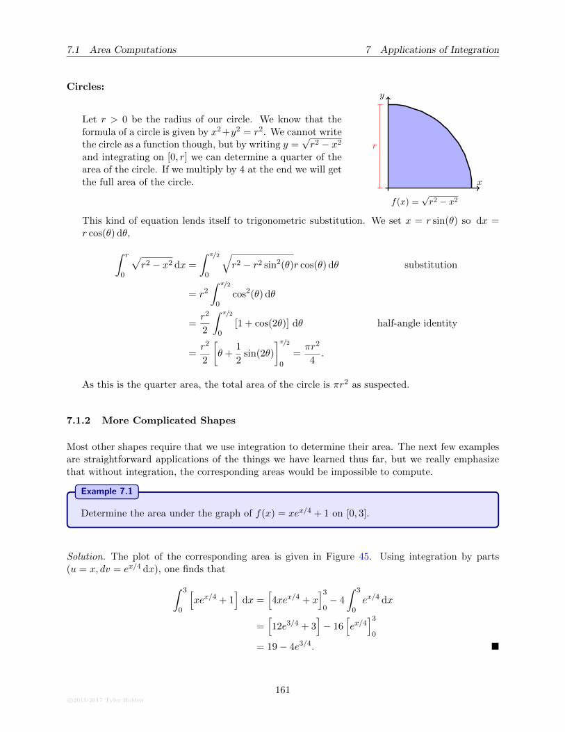
7.1 Area Computations 7 Applications of Integration
Circles:
Let r > 0 be the radius of our circle. We know that theformula of a circle is given by x2 +y2 = r2. We cannot writethe circle as a function though, but by writing y =
√r2 − x2
and integrating on [0, r] we can determine a quarter of thearea of the circle. If we multiply by 4 at the end we will getthe full area of the circle.
f(x) =√r2 − x2
x
y
r
This kind of equation lends itself to trigonometric substitution. We set x = r sin(θ) so dx =r cos(θ) dθ,
∫ r
0
√r2 − x2 dx =
∫ π/2
0
√r2 − r2 sin2(θ)r cos(θ) dθ substitution
= r2
∫ π/2
0cos2(θ) dθ
=r2
2
∫ π/2
0[1 + cos(2θ)] dθ half-angle identity
=r2
2
[θ +
1
2sin(2θ)
]π/2
0
=πr2
4.
As this is the quarter area, the total area of the circle is πr2 as suspected.
7.1.2 More Complicated Shapes
Most other shapes require that we use integration to determine their area. The next few examplesare straightforward applications of the things we have learned thus far, but we really emphasizethat without integration, the corresponding areas would be impossible to compute.
Example 7.1
Determine the area under the graph of f(x) = xex/4 + 1 on [0, 3].
Solution. The plot of the corresponding area is given in Figure 45. Using integration by parts(u = x, dv = ex/4 dx), one finds that
∫ 3
0
[xex/4 + 1
]dx =
[4xex/4 + x
]3
0− 4
∫ 3
0ex/4 dx
=[12e3/4 + 3
]− 16
[ex/4
]3
0
= 19− 4e3/4. �
c©2013-2017 Tyler Holden
161

7 Applications of Integration 7.1 Area Computations
f(x) =
xex/4 + 2
1 2 3
2
4
6
Figure 45: A relatively simple shape whose area is difficult to compute.
Example 7.2
Determine the area under the graph of f(x) =sin(
3πx
)
x2on the interval [0.15, 0.5].
0.2 0.25 0.3 0.35 0.4 0.45 0.5
−20
20
x
y
Figure 46: A function which is rapidly oscillating.
Solution. The corresponding plot is drawn in Figure 46. We proceed by integrating with a simplesubstitution u = 3π
x to get
∫ 0.5
0.15
sin(
3πx
)
x2dx = − 1
3π
∫ 6π
20πsin(u) du
=1
3πcos(u)|6π20π = 0.
This is rather interesting. It is clear that adjacent areas are very similar in shape, but not equal.Nonetheless, the areas managed to completely cancel one another out. �
7.1.3 Unsigned (Absolute) Area
By now we are quite familiar with the fact that integrals compute signed areas; that is, areas abovethe x-axis are given positive sign, while those beneath the x-axis carry a negative sign. As such, it
162c©2013-2017 Tyler Holden
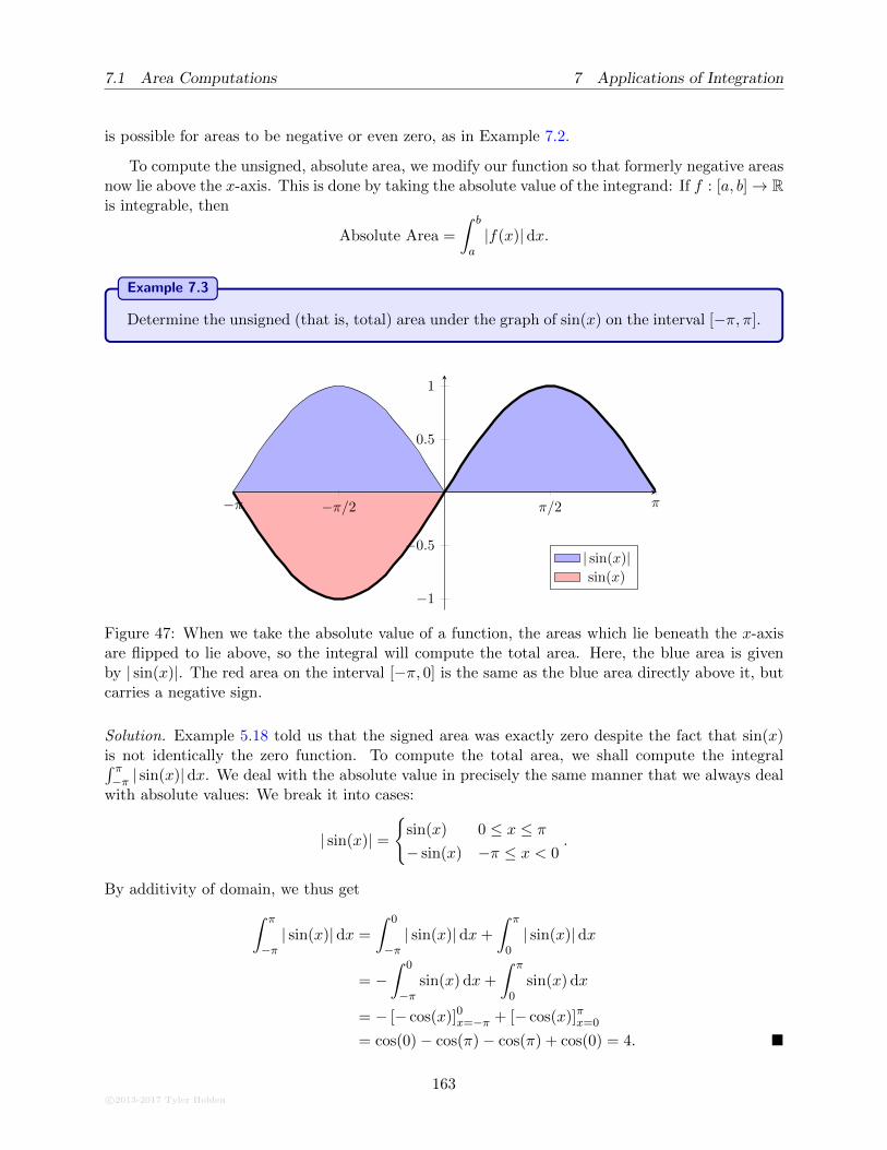
7.1 Area Computations 7 Applications of Integration
is possible for areas to be negative or even zero, as in Example 7.2.
To compute the unsigned, absolute area, we modify our function so that formerly negative areasnow lie above the x-axis. This is done by taking the absolute value of the integrand: If f : [a, b]→ Ris integrable, then
Absolute Area =
∫ b
a|f(x)| dx.
Example 7.3
Determine the unsigned (that is, total) area under the graph of sin(x) on the interval [−π, π].
−π −π/2 π/2 π
−1
−0.5
0.5
1
| sin(x)|sin(x)
Figure 47: When we take the absolute value of a function, the areas which lie beneath the x-axisare flipped to lie above, so the integral will compute the total area. Here, the blue area is givenby | sin(x)|. The red area on the interval [−π, 0] is the same as the blue area directly above it, butcarries a negative sign.
Solution. Example 5.18 told us that the signed area was exactly zero despite the fact that sin(x)is not identically the zero function. To compute the total area, we shall compute the integral∫ π−π | sin(x)| dx. We deal with the absolute value in precisely the same manner that we always deal
with absolute values: We break it into cases:
| sin(x)| ={
sin(x) 0 ≤ x ≤ π− sin(x) −π ≤ x < 0
.
By additivity of domain, we thus get
∫ π
−π| sin(x)| dx =
∫ 0
−π| sin(x)|dx+
∫ π
0| sin(x)| dx
= −∫ 0
−πsin(x) dx+
∫ π
0sin(x) dx
= − [− cos(x)]0x=−π + [− cos(x)]πx=0
= cos(0)− cos(π)− cos(π) + cos(0) = 4. �
c©2013-2017 Tyler Holden
163
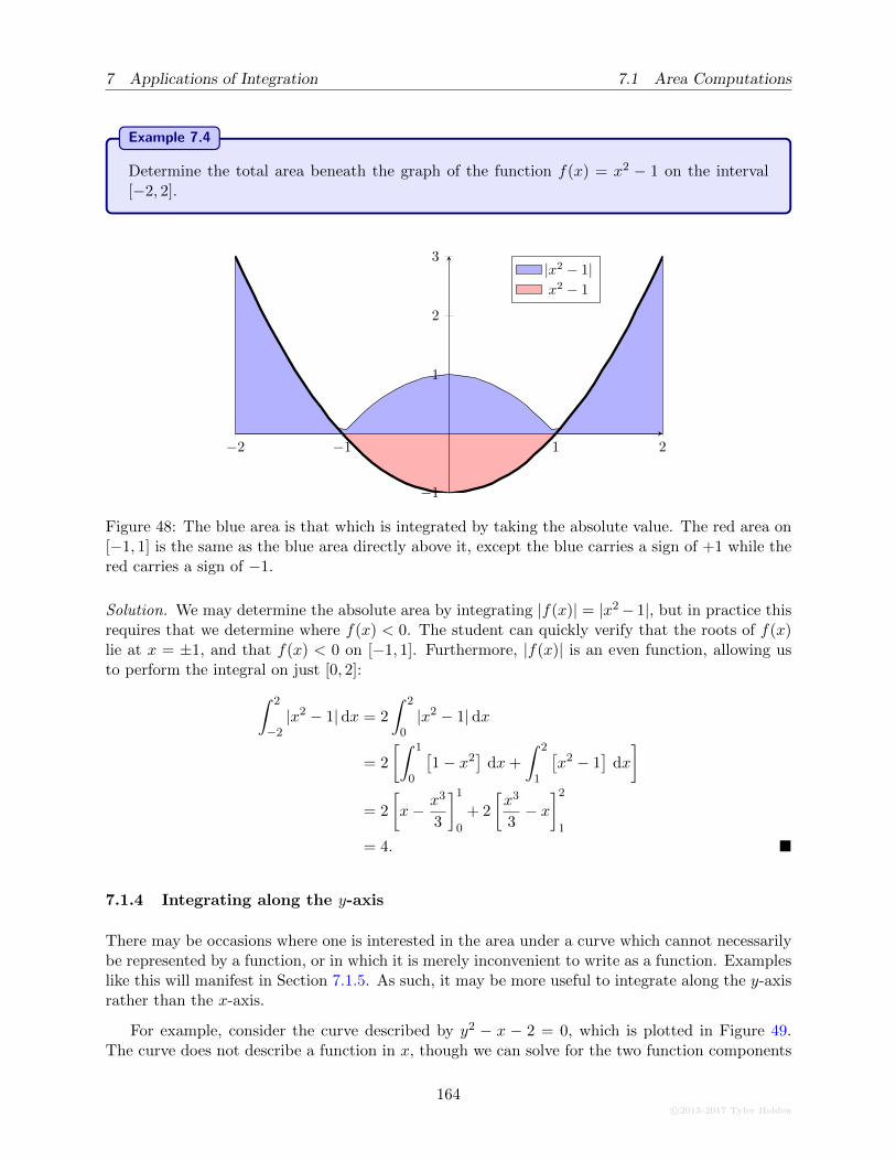
7 Applications of Integration 7.1 Area Computations
Example 7.4
Determine the total area beneath the graph of the function f(x) = x2 − 1 on the interval[−2, 2].
−2 −1 1 2
−1
1
2
3|x2 − 1|x2 − 1
Figure 48: The blue area is that which is integrated by taking the absolute value. The red area on[−1, 1] is the same as the blue area directly above it, except the blue carries a sign of +1 while thered carries a sign of −1.
Solution. We may determine the absolute area by integrating |f(x)| = |x2− 1|, but in practice thisrequires that we determine where f(x) < 0. The student can quickly verify that the roots of f(x)lie at x = ±1, and that f(x) < 0 on [−1, 1]. Furthermore, |f(x)| is an even function, allowing usto perform the integral on just [0, 2]:
∫ 2
−2|x2 − 1|dx = 2
∫ 2
0|x2 − 1|dx
= 2
[∫ 1
0
[1− x2
]dx+
∫ 2
1
[x2 − 1
]dx
]
= 2
[x− x3
3
]1
0
+ 2
[x3
3− x]2
1
= 4. �
7.1.4 Integrating along the y-axis
There may be occasions where one is interested in the area under a curve which cannot necessarilybe represented by a function, or in which it is merely inconvenient to write as a function. Exampleslike this will manifest in Section 7.1.5. As such, it may be more useful to integrate along the y-axisrather than the x-axis.
For example, consider the curve described by y2 − x − 2 = 0, which is plotted in Figure 49.The curve does not describe a function in x, though we can solve for the two function components
164c©2013-2017 Tyler Holden
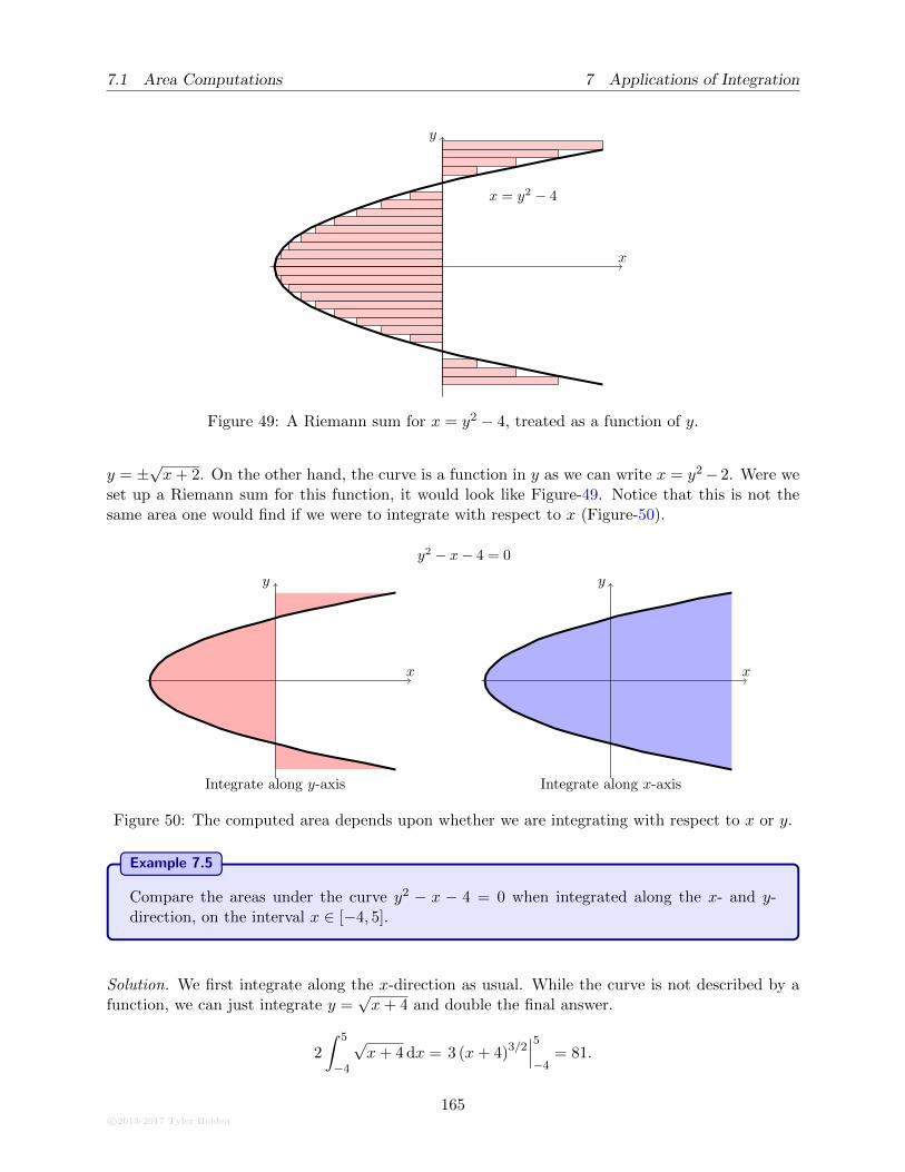
7.1 Area Computations 7 Applications of Integration
x = y2 − 4
x
y
Figure 49: A Riemann sum for x = y2 − 4, treated as a function of y.
y = ±√x+ 2. On the other hand, the curve is a function in y as we can write x = y2− 2. Were we
set up a Riemann sum for this function, it would look like Figure-49. Notice that this is not thesame area one would find if we were to integrate with respect to x (Figure-50).
x
y
Integrate along y-axis
y2 − x− 4 = 0
x
y
Integrate along x-axis
Figure 50: The computed area depends upon whether we are integrating with respect to x or y.
Example 7.5
Compare the areas under the curve y2 − x − 4 = 0 when integrated along the x- and y-direction, on the interval x ∈ [−4, 5].
Solution. We first integrate along the x-direction as usual. While the curve is not described by afunction, we can just integrate y =
√x+ 4 and double the final answer.
2
∫ 5
−4
√x+ 4 dx = 3 (x+ 4)3/2
∣∣∣5
−4= 81.
c©2013-2017 Tyler Holden
165
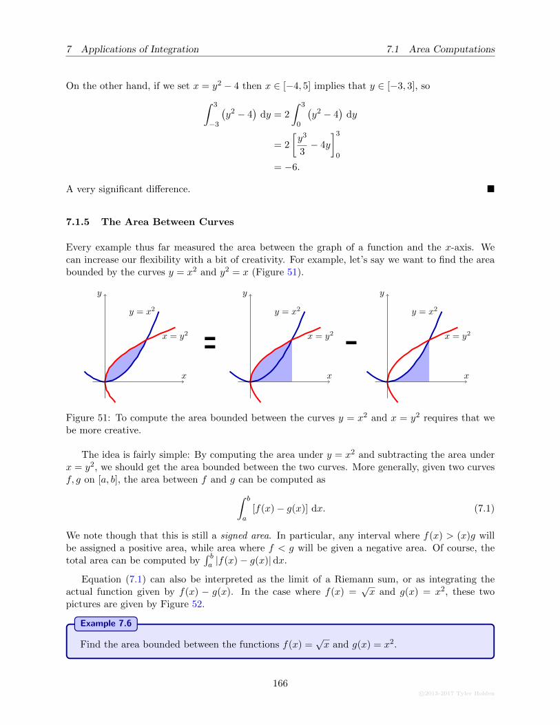
7 Applications of Integration 7.1 Area Computations
On the other hand, if we set x = y2 − 4 then x ∈ [−4, 5] implies that y ∈ [−3, 3], so
∫ 3
−3
(y2 − 4
)dy = 2
∫ 3
0
(y2 − 4
)dy
= 2
[y3
3− 4y
]3
0
= −6.
A very significant difference. �
7.1.5 The Area Between Curves
Every example thus far measured the area between the graph of a function and the x-axis. Wecan increase our flexibility with a bit of creativity. For example, let’s say we want to find the areabounded by the curves y = x2 and y2 = x (Figure 51).
y = x2
x = y2
x
y
y = x2
x = y2
x
y
y = x2
x = y2
x
y
Figure 51: To compute the area bounded between the curves y = x2 and x = y2 requires that webe more creative.
The idea is fairly simple: By computing the area under y = x2 and subtracting the area underx = y2, we should get the area bounded between the two curves. More generally, given two curvesf, g on [a, b], the area between f and g can be computed as
∫ b
a[f(x)− g(x)] dx. (7.1)
We note though that this is still a signed area. In particular, any interval where f(x) > (x)g willbe assigned a positive area, while area where f < g will be given a negative area. Of course, thetotal area can be computed by
∫ ba |f(x)− g(x)|dx.
Equation (7.1) can also be interpreted as the limit of a Riemann sum, or as integrating theactual function given by f(x) − g(x). In the case where f(x) =
√x and g(x) = x2, these two
pictures are given by Figure 52.
Example 7.6
Find the area bounded between the functions f(x) =√x and g(x) = x2.
166c©2013-2017 Tyler Holden
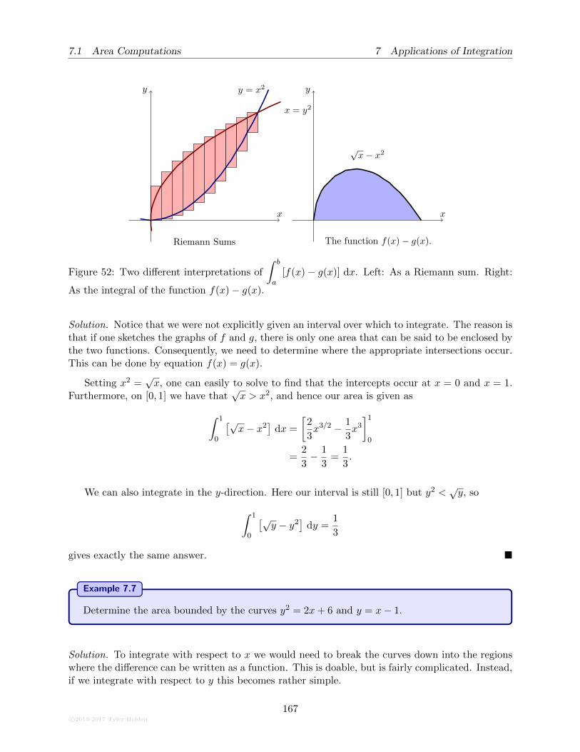
7.1 Area Computations 7 Applications of Integration
y = x2
x = y2
x
y
Riemann Sums
x
y
√x− x2
The function f(x)− g(x).
Figure 52: Two different interpretations of
∫ b
a[f(x)− g(x)] dx. Left: As a Riemann sum. Right:
As the integral of the function f(x)− g(x).
Solution. Notice that we were not explicitly given an interval over which to integrate. The reason isthat if one sketches the graphs of f and g, there is only one area that can be said to be enclosed bythe two functions. Consequently, we need to determine where the appropriate intersections occur.This can be done by equation f(x) = g(x).
Setting x2 =√x, one can easily to solve to find that the intercepts occur at x = 0 and x = 1.
Furthermore, on [0, 1] we have that√x > x2, and hence our area is given as
∫ 1
0
[√x− x2
]dx =
[2
3x3/2 − 1
3x3
]1
0
=2
3− 1
3=
1
3.
We can also integrate in the y-direction. Here our interval is still [0, 1] but y2 <√y, so
∫ 1
0
[√y − y2
]dy =
1
3
gives exactly the same answer. �
Example 7.7
Determine the area bounded by the curves y2 = 2x+ 6 and y = x− 1.
Solution. To integrate with respect to x we would need to break the curves down into the regionswhere the difference can be written as a function. This is doable, but is fairly complicated. Instead,if we integrate with respect to y this becomes rather simple.
c©2013-2017 Tyler Holden
167
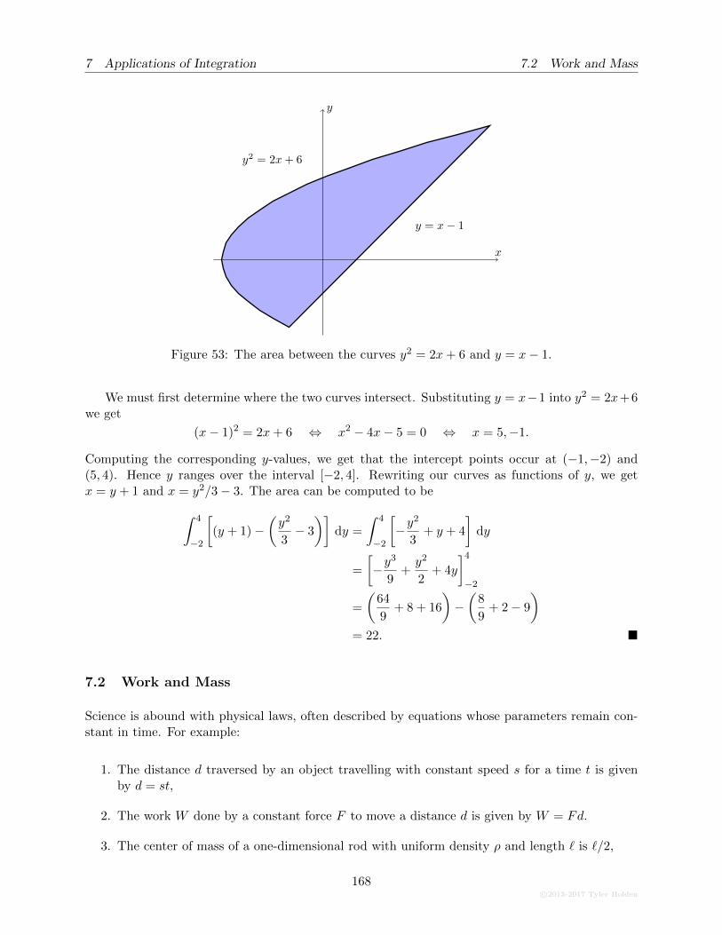
7 Applications of Integration 7.2 Work and Mass
x
y
y = x− 1
y2 = 2x+ 6
Figure 53: The area between the curves y2 = 2x+ 6 and y = x− 1.
We must first determine where the two curves intersect. Substituting y = x−1 into y2 = 2x+6we get
(x− 1)2 = 2x+ 6 ⇔ x2 − 4x− 5 = 0 ⇔ x = 5,−1.
Computing the corresponding y-values, we get that the intercept points occur at (−1,−2) and(5, 4). Hence y ranges over the interval [−2, 4]. Rewriting our curves as functions of y, we getx = y + 1 and x = y2/3− 3. The area can be computed to be
∫ 4
−2
[(y + 1)−
(y2
3− 3
)]dy =
∫ 4
−2
[−y
2
3+ y + 4
]dy
=
[−y
3
9+y2
2+ 4y
]4
−2
=
(64
9+ 8 + 16
)−(
8
9+ 2− 9
)
= 22. �
7.2 Work and Mass
Science is abound with physical laws, often described by equations whose parameters remain con-stant in time. For example:
1. The distance d traversed by an object travelling with constant speed s for a time t is givenby d = st,
2. The work W done by a constant force F to move a distance d is given by W = Fd.
3. The center of mass of a one-dimensional rod with uniform density ρ and length ` is `/2,
168c©2013-2017 Tyler Holden
7.2 Work and Mass 7 Applications of Integration
These equations are very nice, but represent idealized situations. For example, what happensto our distance formula d = st if our speed is allowed to vary with time? Similarly, our force Fmay vary with distance or our density ρ might not be uniform. When we allow objects to behavedynamically, we are forced to employ calculus.
We have already addressed the problem of calculating distance with variable speed; in fact, thiswas our motivational problem presented in Section 5.2.1. If s(t) describes the speed of a particleas a function of time t, we can estimate the total distance travelled by breaking the interval [t0, t1]into smaller time intervals, then approximating the speed by choosing a sampling of s on eachsubinterval. For example, if we choose to take n-uniform intervals of length ∆t, and approximates on each subinterval by the speed at the beginning of the interval, then
approximate distance =
n−1∑
k=0
s
(t1 − t0n
k
)∆t,
which we recognize as the left Riemann sum. The true distance travelled manifests as we take thelimit ∆t→ 0, yielding a total distance
d =
∫ t1
t0
s(t) dt.
We will implement the same strategy to determine the resolution for our other hypothesized sce-narios, when density and force are allowed to vary with time.
Remark 7.8 We emphasize that we have chosen work and mass as representative examplesonly. The strategies developed in the following sections are meant to be generalized by thereader to arbitrary situations, whenever needed.
7.2.1 Work
Deriving the formula for work dependent upon a variable force will almost be identical to thederivation of distance subject to variable speed. Nonetheless, it is important to see how suchderivations are done mathematically, so we begin with this simple example to reinforce the logicalprocess.
Consider a particle, acted upon by a force F . If the force is constant in time, and the particleis displaced by an amount s, then the work W done on the particle by the force F is given byW = Fs. The SI-units for force are Newtons, while work is given by Joules = Newtons · seconds.More realistically, force often varies either with respect to distance s, time t, or both. For example,the force of gravity exerted by the sun is significantly greater on Mercury than on Jupiter as a resultof the distances of these planets to the sun. On the other hand, an electric motor on an alternatingcurrent experiences a time-dependent force, arising from the change in polarity of a magnetic field.
Our goal now is to consider the correct equation for W when our force is allowed to vary. Let’sassume that F (x) is a continuous function of the displacement s on [0, sf ], where sf > 0 is the finaldisplacement of the particle. We can approximate the work exerted by the force on the particle bybreaking [0, sf ] into sub-intervals, approximating F by a constant on each such interval, and usingthe equation W = Fs on each of these intervals.
c©2013-2017 Tyler Holden
169
7 Applications of Integration 7.2 Work and Mass
To this effect, we partition [0, sf ] into n equal length subintervals, with ∆s = sf/n, and choosea sampling ti ∈ [i∆s, (i + 1)∆s]. The approximate work done on the interval [i∆s, (i + 1)∆s] isthen given by Wi = F (ti)∆s, so the total work is approximated by
approximate work =
n∑
k=1
Wi =
n∑
k=1
F (ti)∆s.
This is just a Riemann sum! The total work is then found by taking the limit as our partitionintervals become infinitesimally small. Since F is continuous it is integrable, implying that thelimit will converge, so we conclude that
W =
∫ sf
0F (s) ds. (7.2)
Displacement versus Distance: Our integral above is in terms of the displacement of theparticle; that is, the total distance the particle has travelled from its starting position. However,displacement is relative to the particle, while forces are typically more absolute, making displace-ment an inconvenient unit in which to express force. For example, a particle at the point x on thereal line might experience a force of F (x) = 2/x2 Newtons. If the particle starts at x = 5 and findsitself at x = 7, then its displacement is s = 2. The force it feels at s = 2 corresponds to x = 7though, so clearly our units s and x do not agree.
The relationship between displacement and distance is straightforward: If x0 is the initiallocation of the particle, then s = x− x0. One solution is therefore to write the force F in terms ofs, giving F (x) = F (s+ x0), which can be substituted into (7.2) and integrated to find the answer.Alternatively, we can perform a change of variables! Since s = x− x0 we know that ds = dx, andso
W =
∫ sf
0F (s) ds =
∫ x0+sf
x0
F (x) dx.
Example 7.9
A particle at position x ∈ R is acted upon by a force of F (x) = 2/x2 N. If the particle beginsat x0 = 5 and finishes at x = 7, determine the work done by the force on the particle.
Solution. Our particle experiences a displacement of sf = 2. As mentioned above, we know thatthe relationship between s and x is given by s = x − x0 = x − 5. Rewriting F in terms of thedisplacement, we have F (x) = F (s+ 5) = 2/(x+ 5)2, so that
W =
∫ 2
0F (s+ 5) ds =
∫ 2
0
2
(x+ 5)2ds = − 2
x+ 5
∣∣∣∣2
0
=4
35Joules.
Alternatively, we can integrate using the change of variable method, to find
W =
∫ 7
5
2
x2dx = − 2
x
∣∣∣∣7
5
=4
35Joules. �
170c©2013-2017 Tyler Holden
7.2 Work and Mass 7 Applications of Integration
There are many variations one could employ to change the dynamics of our problem. Forexample, the force F could vary upon time t but not upon distance. In this instance, our integralformula changes. Alternatively, consider an instance where a particle is moving in two dimensions.If F is a force which acts only in the x-direction, then the effective force felt by the particle isF cos(θ), where θ is the angle made by the tangent vector to the curve and the x-axis. A fulltreatment of this scenario requires multi-variable calculus, but one could imagine being given θ asa function of time, and being told to determine the work. These are examples that will be takenup in the exercises.
7.2.2 Mass
The study of mass will yield several important results. Most obviously, mass is an importantquantity in physics and warrants discussion on those grounds alone. However, more pertinent toour study will be the technique used to compute the center of mass for one- and two-dimensionalspaces.
We begin with the problem of determining the mass of a one-dimensional rod of length `,composed of a material with density ρ. In a single dimension, density measures how much massoccurs per unit length; therefore, if the rod has a uniform density ρ the total mass will be m = ρ`.If the density is allowed to vary with the length of the rod, the total mass may be computed in amanner almost identical to what was considered in section 7.2.1. In the exercise below, the studentwill show that if a rod is placed on the x-axis with one endpoint at x = 0 and the other at x = `,then the total mass of the rod will be
m =
∫ `
0ρ(x) dx, (7.3)
where the density ρ now varies as a function of the length of the rod.
Exercise: (Mass of a Rod) Show that if a rod of length ` is composed of a material withdensity ρ(x), 0 ≤ x ≤ `, then the mass of the rod is given by (7.3).
Let’s try something new: The center of mass of an object is the unique point of an object wherethe mass is equally distributed in all possible directions. In effect, one can always balance an objectby positioning the fulcrum at the center of mass. One can often utilize the center of mass to reducedifficult computations involving a large object to that of a single point.
For a one-dimensional rod of uniform mass-density ρ, spanning the interval [a, b], the center ofmass will be located at the center of the interval; namely, CoM = (a + b)/2. Notice that in thiscase the density plays no role in determining the center of mass. How do we extend this notionto multiple different rods? Consider a collection of rods, who have centers of mass located at{x1, . . . , xn} and mass {m1, . . . ,mn}. The center of mass of the combined system will be given by
CoM =1
m1 + · · ·+mn
n∑
i=1
ximi. (7.4)
Take a moment and convince yourself that this makes sense. For example, if a marble with mass 1gram is located at x = −1 and a marble of mass 1 gram is located at x = +1, then the center of
c©2013-2017 Tyler Holden
171
7 Applications of Integration 7.3 Cross Sections
mass should be at x = 0. However, if we increase the mass of the second marble to x = 2 grams,then the mass should be at x = 1/3, owing to the fact that the second marble is heavier.
We can use (7.4) to build an integral expression for the center of mass of a rod with continuouslyvarying mass-density ρ. Assume the rod is placed so that one end is at x = 0 and the other is atx = `. We will approximate the center of mass by breaking the rod into smaller rods, choosing asample of ρ on each smaller rod, and then summing according to (7.4). Partition [0, `] into n equalsubintervals, with ∆x = `/n and tags ti ∈ [i∆x, (i + 1)∆x]. Each smaller rod on [i∆x, (i + 1)∆x]has an approximate total mass of mi = ρ(ti)∆x, so that the center of mass of the n rods is
Approximate CoM =1
m1 + · · ·+mn
n∑
i=1
(xi−1 + xi
2
)ρ(ti)∆x.
=1
M
n∑
i=1
xi−1
2ρ(ti)∆x
︸ ︷︷ ︸(I)
+1
M
n∑
i=1
xi2ρ(ti)∆xi
︸ ︷︷ ︸(II)
.
Term (II) is a proper Riemann sum for the function x2ρ(x), and will converge if ρ is integrable.
Term (I) is not a Riemman sum, but we know that it converges to the integral for x2ρ(x) by Bliss’
Theorem. We conclude that the center of mass is given by
Center of Mass =
[∫ `
0ρ(x) dx
]−1 [∫ `
0xρ(x) dx
],
which is the continuous version of the sum given in (7.4).
Example 7.10
Calculate the center of mass for a rod spanning [−1, 1] with a mass-density given by ρ(x) =1− x3.
Solution. We could choose to move our bar so as to be position along the interval [0, 2], but as themass density is in terms of x ∈ [−1, 1], it is easiest just to leave the system as it is. We begin bycomputing the mass of the rod,
M =
∫ 1
−1ρ(x) dx =
∫ 1
−1[1− x3] dx = 2.
Next, we compute the integral over xρ(x), which gives
∫ 1
−1xρ(x) dx =
∫ 1
−1[x− x4] dx = −2
5.
Thus the center of mass is located at x = −1/5. �
7.3 Cross Sections
Beyond two dimensional area lies three dimensional volume. In general, we will need to developthe theory of multivariate integration to compute volumes. However, if one is presented with a
172c©2013-2017 Tyler Holden
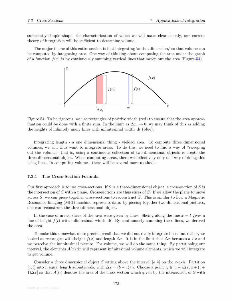
7.3 Cross Sections 7 Applications of Integration
sufficiently simple shape, the characterization of which we will make clear shortly, our currenttheory of integration will be sufficient to determine volume.
The major theme of this entire section is that integrating ‘adds a dimension,’ so that volume canbe computed by integrating area. One way of thinking about computing the area under the graphof a function f(x) is by continuously summing vertical lines that sweep out the area (Figure-54).
x
y
f(ti)
∆xi
f(t)
dt
f(x)
Figure 54: To be rigorous, we use rectangles of positive width (red) to ensure that the area approx-imation could be done with a finite sum. In the limit as ∆xi → 0, we may think of this as addingthe heights of infinitely many lines with infinitesimal width dt (blue).
Integrating length - a one dimensional thing - yielded area. To compute three dimensionalvolumes, we will thus want to integrate areas. To do this, we need to find a way of “sweepingout the volume;” that is, using a continuous collection of two-dimensional objects re-create thethree-dimensional object. When computing areas, there was effectively only one way of doing thisusing lines. In computing volumes, there will be several more methods.
7.3.1 The Cross-Section Formula
Our first approach is to use cross-sections. If S is a three-dimensional object, a cross-section of S isthe intersection of S with a plane. Cross-sections are thus slices of S. If we allow the plane to moveacross S, we can piece together cross-sections to reconstruct S. This is similar to how a MagneticResonance Imaging (MRI) machine represents data: by piecing together two dimensional pictures,one can reconstruct the three dimensional object.
In the case of areas, slices of the area were given by lines. Slicing along the line x = t gives aline of height f(t) with infinitesimal width dt. By continuously summing these lines, we derivedthe area.
To make this somewhat more precise, recall that we did not really integrate lines, but rather, welooked at rectangles with height f(x) and length ∆x. It is in the limit that ∆x becomes a dx andwe perceive the infinitesimal picture. For volume, we will do the same thing. By partitioning ourinterval, the elements A(x) dx will represent infinitesimal volume elements, which we will integrateto get volume.
Consider a three dimensional object S sitting above the interval [a, b] on the x-axis. Partition[a, b] into n equal length subintervals, with ∆x = (b− a)/n. Choose a point ti ∈ [a+ i∆x, a+ (i+1)∆x] so that A(ti) denotes the area of the cross section which given by the intersection of S with
c©2013-2017 Tyler Holden
173
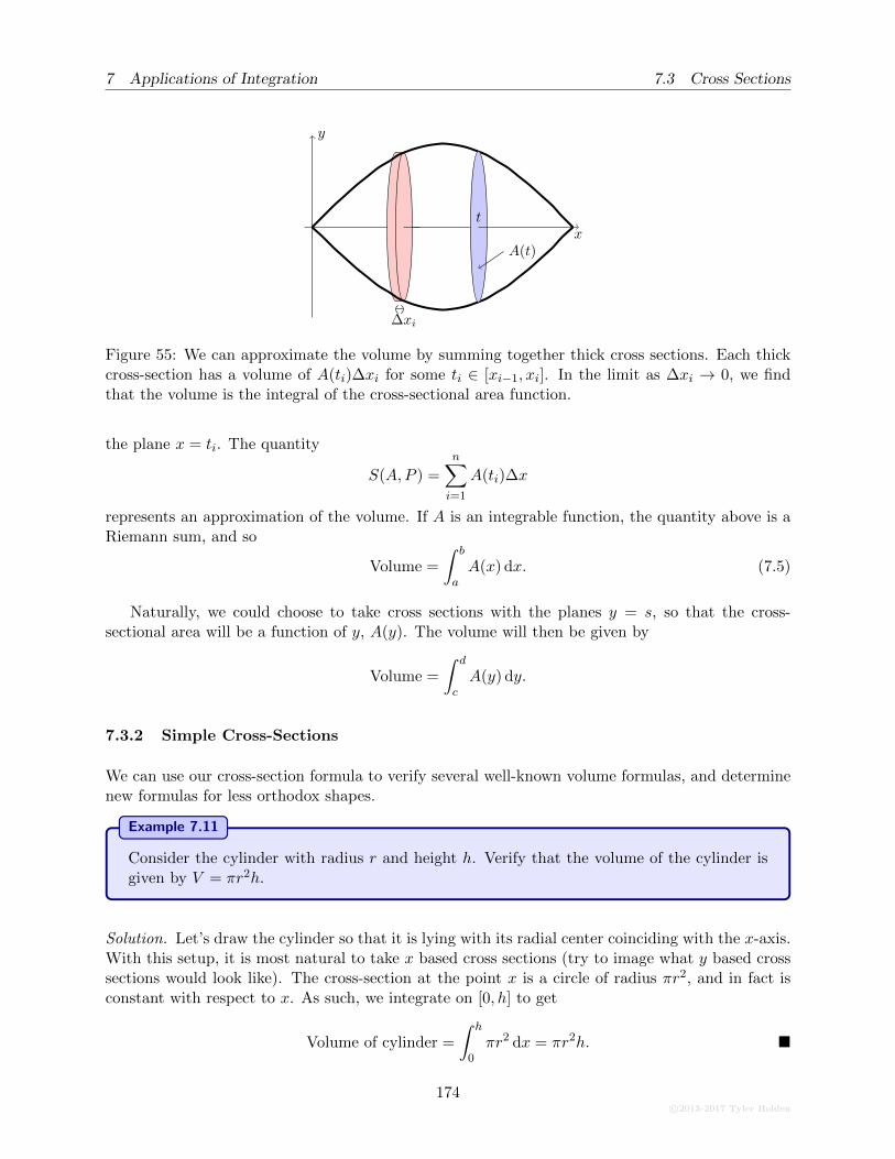
7 Applications of Integration 7.3 Cross Sections
x
y
∆xi
t
A(t)
Figure 55: We can approximate the volume by summing together thick cross sections. Each thickcross-section has a volume of A(ti)∆xi for some ti ∈ [xi−1, xi]. In the limit as ∆xi → 0, we findthat the volume is the integral of the cross-sectional area function.
the plane x = ti. The quantity
S(A,P ) =n∑
i=1
A(ti)∆x
represents an approximation of the volume. If A is an integrable function, the quantity above is aRiemann sum, and so
Volume =
∫ b
aA(x) dx. (7.5)
Naturally, we could choose to take cross sections with the planes y = s, so that the cross-sectional area will be a function of y, A(y). The volume will then be given by
Volume =
∫ d
cA(y) dy.
7.3.2 Simple Cross-Sections
We can use our cross-section formula to verify several well-known volume formulas, and determinenew formulas for less orthodox shapes.
Example 7.11
Consider the cylinder with radius r and height h. Verify that the volume of the cylinder isgiven by V = πr2h.
Solution. Let’s draw the cylinder so that it is lying with its radial center coinciding with the x-axis.With this setup, it is most natural to take x based cross sections (try to image what y based crosssections would look like). The cross-section at the point x is a circle of radius πr2, and in fact isconstant with respect to x. As such, we integrate on [0, h] to get
Volume of cylinder =
∫ h
0πr2 dx = πr2h. �
174c©2013-2017 Tyler Holden
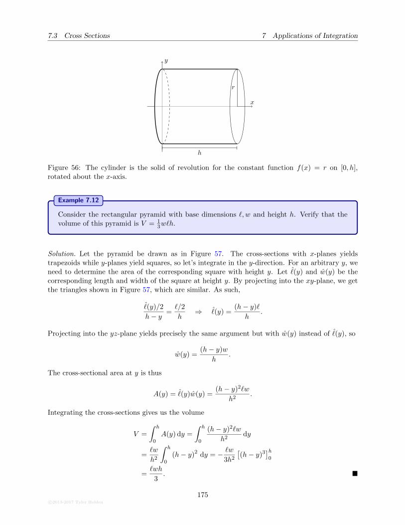
7.3 Cross Sections 7 Applications of Integration
x
y
h
r
Figure 56: The cylinder is the solid of revolution for the constant function f(x) = r on [0, h],rotated about the x-axis.
Example 7.12
Consider the rectangular pyramid with base dimensions `, w and height h. Verify that thevolume of this pyramid is V = 1
3w`h.
Solution. Let the pyramid be drawn as in Figure 57. The cross-sections with x-planes yieldstrapezoids while y-planes yield squares, so let’s integrate in the y-direction. For an arbitrary y, weneed to determine the area of the corresponding square with height y. Let ˆ(y) and w(y) be thecorresponding length and width of the square at height y. By projecting into the xy-plane, we getthe triangles shown in Figure 57, which are similar. As such,
ˆ(y)/2
h− y =`/2
h⇒ ˆ(y) =
(h− y)`
h.
Projecting into the yz-plane yields precisely the same argument but with w(y) instead of ˆ(y), so
w(y) =(h− y)w
h.
The cross-sectional area at y is thus
A(y) = ˆ(y)w(y) =(h− y)2`w
h2.
Integrating the cross-sections gives us the volume
V =
∫ h
0A(y) dy =
∫ h
0
(h− y)2`w
h2dy
=`w
h2
∫ h
0(h− y)2 dy = − `w
3h2
[(h− y)3
]h0
=`wh
3. �
c©2013-2017 Tyler Holden
175
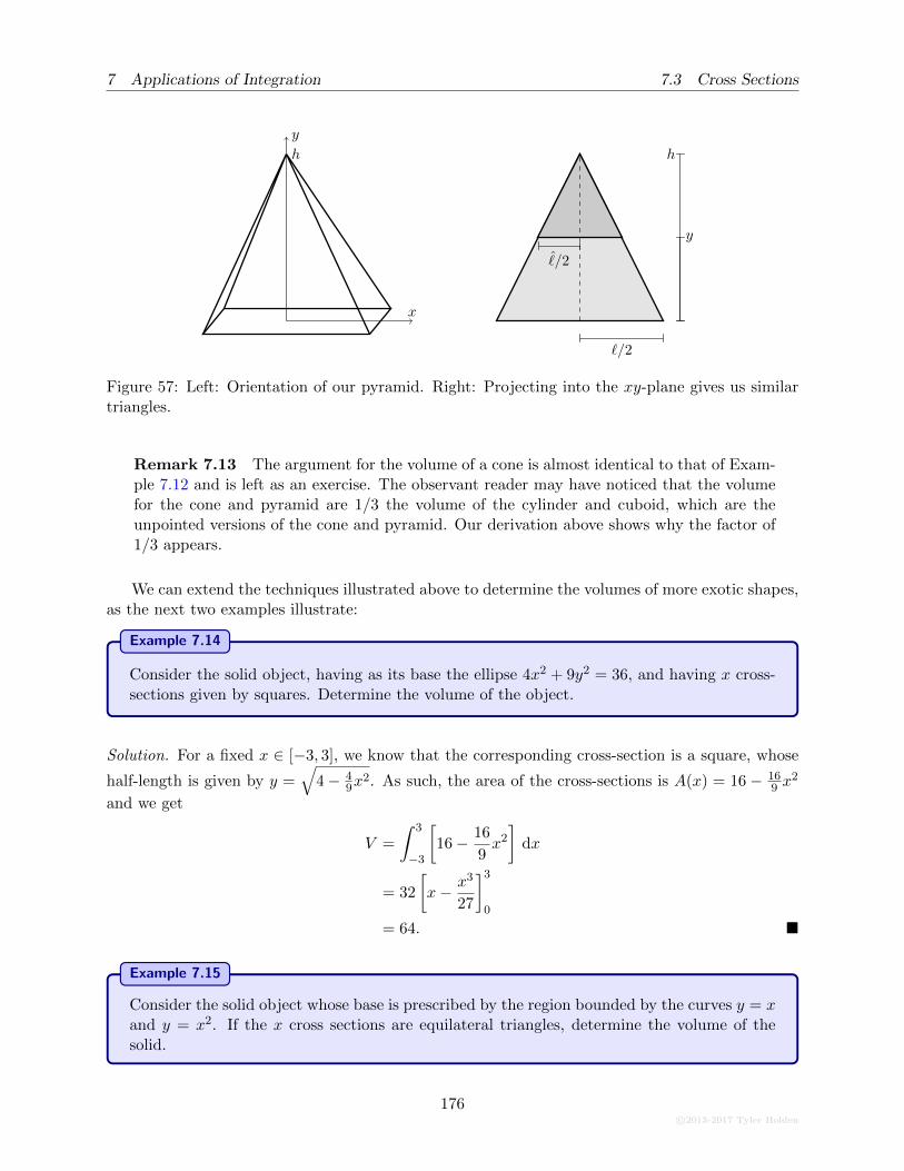
7 Applications of Integration 7.3 Cross Sections
y
x
h
`/2
ˆ/2
h
y
Figure 57: Left: Orientation of our pyramid. Right: Projecting into the xy-plane gives us similartriangles.
Remark 7.13 The argument for the volume of a cone is almost identical to that of Exam-ple 7.12 and is left as an exercise. The observant reader may have noticed that the volumefor the cone and pyramid are 1/3 the volume of the cylinder and cuboid, which are theunpointed versions of the cone and pyramid. Our derivation above shows why the factor of1/3 appears.
We can extend the techniques illustrated above to determine the volumes of more exotic shapes,as the next two examples illustrate:
Example 7.14
Consider the solid object, having as its base the ellipse 4x2 + 9y2 = 36, and having x cross-sections given by squares. Determine the volume of the object.
Solution. For a fixed x ∈ [−3, 3], we know that the corresponding cross-section is a square, whose
half-length is given by y =√
4− 49x
2. As such, the area of the cross-sections is A(x) = 16− 169 x
2
and we get
V =
∫ 3
−3
[16− 16
9x2
]dx
= 32
[x− x3
27
]3
0
= 64. �
Example 7.15
Consider the solid object whose base is prescribed by the region bounded by the curves y = xand y = x2. If the x cross sections are equilateral triangles, determine the volume of thesolid.
176c©2013-2017 Tyler Holden
7.3 Cross Sections 7 Applications of Integration
Solution. The student can quickly check that y = x and y = x2 intersect at x = 0 and x = 1, sofix an x ∈ [0, 1]. We are told that the cross section is an equilateral triangle, so at x this triangle
has a base of length ` = x−√x. The area of an equilateral triangle with base ` is A =√
34 `
2, so
V =
∫ 1
0
√3
4(x−√x)2 dx
=
√3
4
∫ 1
0
[x2 − 2x3/2 + x
]dx
=
√3
4
[1
3x3 − 4
5x5/2 +
1
2x2
]1
0
=
√3
120. �
7.3.3 Cross-Sections for Solids of Revolution
Symmetry has played an important role in our conversation thus far. The motif of the previoussection was to specify a shape with a given base and highly regular cross-sections. Here we willexplore a different kind of symmetry, wherein our cross-sections are universally given by circles ofvarying radii.
The idea is as follows: Suppose that one specifies a function f with some domain [a, b]. Byrotating that function around the x-axis one generates a “solid of revolution.” Our goal will be tocompute the volumes of such solids.
By virtue of having revolved the function f(x) around the x-axis, cross-sections with respect tothe axis of revolution will yield circles whose radius will be precisely f(x). Thus the cross-sectionalarea as a function of x is A(x) = πf(x)2, and our cross-section formula reads
Volume =
∫ b
aπf(x)2 dx.
Example 7.16
Let f(x) = x2 − 2x + 2 with domain [0, 3] and revolve the graph of f about the x-axis.Determine the corresponding volume of the solid of revolution.
Solution. Taking a cross section at a typical point x, we get a circle whose radius is f(x) =
c©2013-2017 Tyler Holden
177
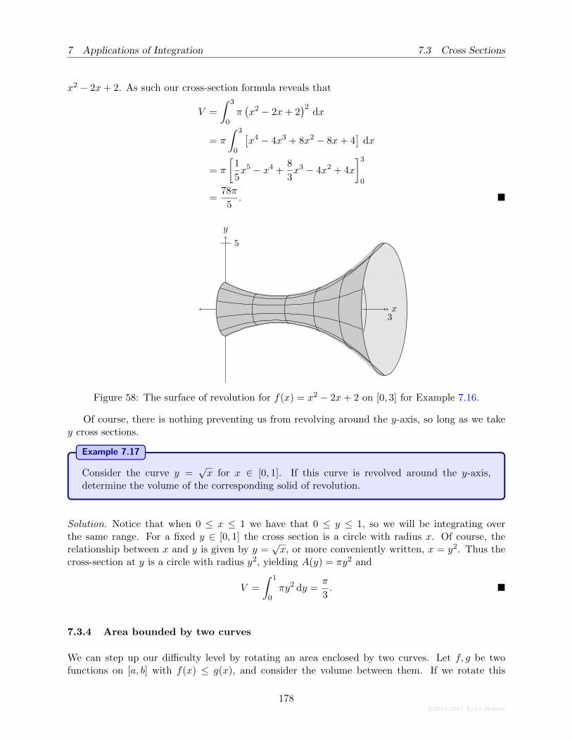
7 Applications of Integration 7.3 Cross Sections
x2 − 2x+ 2. As such our cross-section formula reveals that
V =
∫ 3
0π(x2 − 2x+ 2
)2dx
= π
∫ 3
0
[x4 − 4x3 + 8x2 − 8x+ 4
]dx
= π
[1
5x5 − x4 +
8
3x3 − 4x2 + 4x
]3
0
=78π
5. �
y
x3
5
Figure 58: The surface of revolution for f(x) = x2 − 2x+ 2 on [0, 3] for Example 7.16.
Of course, there is nothing preventing us from revolving around the y-axis, so long as we takey cross sections.
Example 7.17
Consider the curve y =√x for x ∈ [0, 1]. If this curve is revolved around the y-axis,
determine the volume of the corresponding solid of revolution.
Solution. Notice that when 0 ≤ x ≤ 1 we have that 0 ≤ y ≤ 1, so we will be integrating overthe same range. For a fixed y ∈ [0, 1] the cross section is a circle with radius x. Of course, therelationship between x and y is given by y =
√x, or more conveniently written, x = y2. Thus the
cross-section at y is a circle with radius y2, yielding A(y) = πy2 and
V =
∫ 1
0πy2 dy =
π
3. �
7.3.4 Area bounded by two curves
We can step up our difficulty level by rotating an area enclosed by two curves. Let f, g be twofunctions on [a, b] with f(x) ≤ g(x), and consider the volume between them. If we rotate this
178c©2013-2017 Tyler Holden
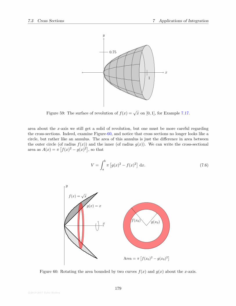
7.3 Cross Sections 7 Applications of Integration
y
x
1
0.75
Figure 59: The surface of revolution of f(x) =√x on [0, 1], for Example 7.17.
area about the x-axis we still get a solid of revolution, but one must be more careful regardingthe cross-sections. Indeed, examine Figure-60, and notice that cross sections no longer looks like acircle, but rather like an annulus. The area of this annulus is just the difference in area betweenthe outer circle (of radius f(x)) and the inner (of radius g(x)). We can write the cross-sectionalarea as A(x) = π
[f(x)2 − g(x)2
], so that
V =
∫ b
aπ[g(x)2 − f(x)2
]dx. (7.6)
x
y
f(x) =√x
g(x) = x
f(x0) g(x0)
Area = π[f(x0)
2 − g(x0)2]
Figure 60: Rotating the area bounded by two curves f(x) and g(x) about the x-axis.
c©2013-2017 Tyler Holden
179
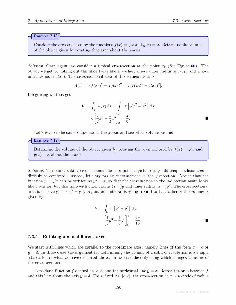
7 Applications of Integration 7.3 Cross Sections
Example 7.18
Consider the area enclosed by the functions f(x) =√x and g(x) = x. Determine the volume
of the object given by rotating that area about the x-axis.
Solution. Once again, we consider a typical cross-section at the point x0 (See Figure 60). Theobject we get by taking out this slice looks like a washer, whose outer radius is f(x0) and whoseinner radius is g(x0). The cross-sectional area of this element is thus
A(x) = πf(x0)2 − πg(x0)2 = π[f(x0)2 − g(x0)2].
Integrating we thus get
V =
∫ 1
0A(x) dx =
∫ 1
0π[√
x2 − x2
]dx
= π
[1
2x2 − 1
3x3
]1
0
=π
6. �
Let’s revolve the same shape about the y-axis and see what volume we find.
Example 7.19
Determine the volume of the object given by rotating the area enclosed by f(x) =√x and
g(x) = x about the y-axis.
Solution. This time, taking cross sections about a point x yields really odd shapes whose area isdifficult to compute. Instead, let’s try taking cross-sections in the y-direction. Notice that thefunction y =
√x can be written as y2 = x, so that the cross section in the y-direction again looks
like a washer, but this time with outer radius (x =)y and inner radius (x =)y2. The cross-sectionalarea is thus A(y) = π[y2 − y4]. Again, our interval is going from 0 to 1, and hence the volume isgiven by
V =
∫ 1
0π[y2 − y4
]dy
=
[1
3y3 − 1
5y5
]1
0
=2π
15. �
7.3.5 Rotating about different axes
We start with lines which are parallel to the coordinate axes; namely, lines of the form x = c ory = d. In these cases the argument for determining the volume of a solid of revolution is a simpleadaptation of what we have discussed above. In essence, the only thing which changes is radius ofthe cross-sections.
Consider a function f defined on [a, b] and the horizontal line y = d. Rotate the area between fand this line about the axis y = d. For a fixed x ∈ [a, b], the cross-section at x is a circle of radius
180c©2013-2017 Tyler Holden
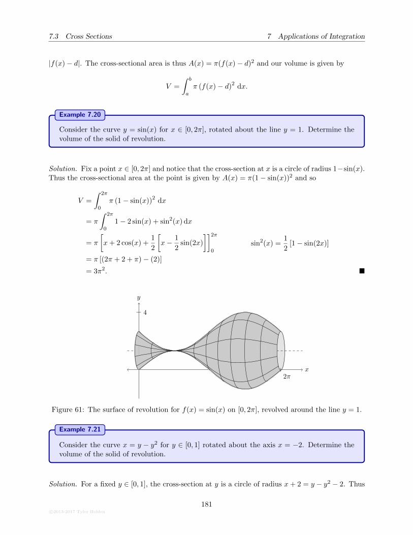
7.3 Cross Sections 7 Applications of Integration
|f(x)− d|. The cross-sectional area is thus A(x) = π(f(x)− d)2 and our volume is given by
V =
∫ b
aπ (f(x)− d)2 dx.
Example 7.20
Consider the curve y = sin(x) for x ∈ [0, 2π], rotated about the line y = 1. Determine thevolume of the solid of revolution.
Solution. Fix a point x ∈ [0, 2π] and notice that the cross-section at x is a circle of radius 1−sin(x).Thus the cross-sectional area at the point is given by A(x) = π(1− sin(x))2 and so
V =
∫ 2π
0π (1− sin(x))2 dx
= π
∫ 2π
01− 2 sin(x) + sin2(x) dx
= π
[x+ 2 cos(x) +
1
2
[x− 1
2sin(2x)
]]2π
0
sin2(x) =1
2[1− sin(2x)]
= π [(2π + 2 + π)− (2)]
= 3π2. �
y
x2π
4
Figure 61: The surface of revolution for f(x) = sin(x) on [0, 2π], revolved around the line y = 1.
Example 7.21
Consider the curve x = y − y2 for y ∈ [0, 1] rotated about the axis x = −2. Determine thevolume of the solid of revolution.
Solution. For a fixed y ∈ [0, 1], the cross-section at y is a circle of radius x+ 2 = y − y2 − 2. Thus
c©2013-2017 Tyler Holden
181
7 Applications of Integration 7.4 Other Volumes
our cross-sectional area is A(y) = π(y − y2 − 2)2 and the volume can be computed as
V =
∫ 1
0π(y2 − y + 2)2 dy
= π
∫ 1
0y4 − 2y3 + 5y2 − 4y + 4 dy
= π
[1
5y5 − 1
2y4 +
5
3y3 − 2y2 + 4y
]1
0
=101π
30. �
As in every case before, we can also look at what happens when we revolve the area betweentwo curves along a non-standard axis.
Example 7.22
Determine the volume of the object given by rotating the area enclosed by f(x) =√x and
g(x) = x about the line x = 1.
Solution. As always, we take a typical cross-section, again in the y-direction this time. We againhave a annulus whose outer radius is 1 − y2 and whose inner radius is 1 − y. The cross sectionalarea is thus
A(y) = π[(1− y2)2 − (1− y)2] = π(2y − 3y2 + y4),
and the volume can be computed as
V = π
∫ 1
0[2y − 3y2 + y4] dy = π
[y2 − y3 +
1
5y5
]1
0
=π
5. �
7.4 Other Volumes
The method of cross-sections is very powerful, but does not represent the only way to get at thevolume of an object. Here we will introduce another method for determining the volume of objects,based off an alternative scheme for sweeping out volume.
7.4.1 Sweeping by Shells
Cross-sections may not always be convenient, resulting in difficult or impossible integrals. Herewe develop a shell-technique, which involves using successively nested cylinder to approximate thevolume. As in the previous sections, the trick is to think about an area, representing an infinitesimalpiece of volume, and sweep out the shape with which we are concerned. For our first example, letf be a function with domain [a, b], and assume that we rotate the area under the graph of f aboutthe y-axis. Choose a point x ∈ [a, b] and consider the cylinder which is centred at the y-axis, withradius x and height f(x). The surface area of this cylinder is given by
S(x) = 2πxf(x).
182c©2013-2017 Tyler Holden
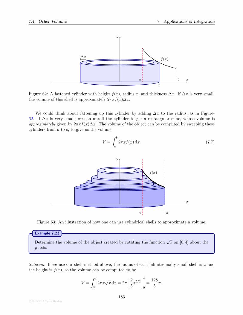
7.4 Other Volumes 7 Applications of Integration
x
y
a b
x
f(x)∆x
Figure 62: A fattened cylinder with height f(x), radius x, and thickness ∆x. If ∆x is very small,the volume of this shell is approximately 2πxf(x)∆x.
We could think about fattening up this cylinder by adding ∆x to the radius, as in Figure-62. If ∆x is very small, we can unroll the cylinder to get a rectangular cube, whose volume isapproximately given by 2πxf(x)∆x. The volume of the object can be computed by sweeping thesecylinders from a to b, to give us the volume
V =
∫ b
a2πxf(x) dx. (7.7)
x
y
a b
f(x)
Figure 63: An illustration of how one can use cylindrical shells to approximate a volume.
Example 7.23
Determine the volume of the object created by rotating the function√x on [0, 4] about the
y-axis.
Solution. If we use our shell-method above, the radius of each infinitesimally small shell is x andthe height is f(x), so the volume can be computed to be
V =
∫ 4
02πx√x dx = 2π
[2
5x5/2
]4
0
=128
5π.
c©2013-2017 Tyler Holden
183
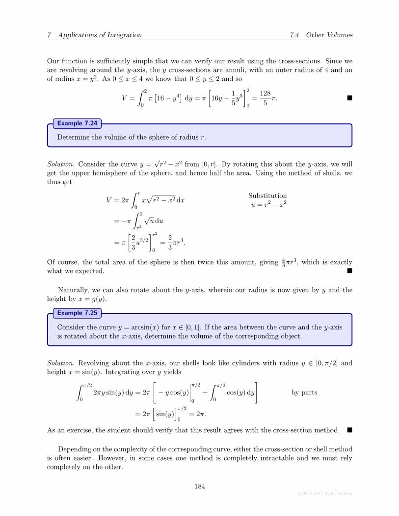
7 Applications of Integration 7.4 Other Volumes
Our function is sufficiently simple that we can verify our result using the cross-sections. Since weare revolving around the y-axis, the y cross-sections are annuli, with an outer radius of 4 and anof radius x = y2. As 0 ≤ x ≤ 4 we know that 0 ≤ y ≤ 2 and so
V =
∫ 2
0π[16− y4
]dy = π
[16y − 1
5y5
]2
0
=128
5π. �
Example 7.24
Determine the volume of the sphere of radius r.
Solution. Consider the curve y =√r2 − x2 from [0, r]. By rotating this about the y-axis, we will
get the upper hemisphere of the sphere, and hence half the area. Using the method of shells, wethus get
V = 2π
∫ r
0x√r2 − x2 dx
Substitution
u = r2 − x2
= −π∫ 0
r2
√udu
= π
[2
3u3/2
]r2
0
=2
3πr3.
Of course, the total area of the sphere is then twice this amount, giving 43πr
3, which is exactlywhat we expected. �
Naturally, we can also rotate about the y-axis, wherein our radius is now given by y and theheight by x = g(y).
Example 7.25
Consider the curve y = arcsin(x) for x ∈ [0, 1]. If the area between the curve and the y-axisis rotated about the x-axis, determine the volume of the corresponding object.
Solution. Revolving about the x-axis, our shells look like cylinders with radius y ∈ [0, π/2] andheight x = sin(y). Integrating over y yields
∫ π/2
02πy sin(y) dy = 2π
[− y cos(y)
∣∣∣∣π/2
0
+
∫ π/2
0cos(y) dy
]by parts
= 2π[
sin(y)]π/2
0= 2π.
As an exercise, the student should verify that this result agrees with the cross-section method. �
Depending on the complexity of the corresponding curve, either the cross-section or shell methodis often easier. However, in some cases one method is completely intractable and we must relycompletely on the other.
184c©2013-2017 Tyler Holden

7.4 Other Volumes 7 Applications of Integration
Example 7.26
Determine the volume when ex2
on [0, 2] is rotated about the y-axis.
Solution. If we were to do this using cross-sections, one would need to solve x as a function ofy. Since x ≥ 0 this can be done to yield x =
√log(y), but this is not a function which is easily
integrated. Instead, if we use the shell method we have cylinders of radius x and height ex2, so that
V =
∫ 2
02πxex
2dx u = x2, du = 2x dx
= π
∫ 4
0eu du = π eu|40 = π(e4 − 1) �
We can easily generalize this process to the case when we have a difference of functions. Forexample, consider the area bounded between two function f(x) and g(x) with f(x) ≤ g(x) on[a, b]. If we look at the cylinder in this case, the radius of the cylinder remains constant, butthe height is given by the difference of the two functions. Hence the surface area is given byS(x) = 2πx[g(x)− f(x)] and the volume becomes
V =
∫ b
a2πx[g(x)− f(x)] dx. (7.8)
Example 7.27
Determine the volume of the object given by rotating the area enclosed between√x and x2
about the y-axis.
Solution. We did this exact problem in Example 7.19 where we got a solution of 2π15 . We certainly
expect that we should get the same solution this time. Again, using the method of shells we get
V =
∫ 1
02πx
[√x− x
]dx = 2π
∫ 1
0
[x3/2 − x2
]dx
= 2π
[2
5x5/2 − 1
3x4
]1
0
=2π
15. �
If we rotate about an axis which is not one of the coordinate axes, then the problem doesnot become too much more complicated. We keep in our mind this incessant picture that we areintegrating using cylinders. Revolving around a different axis now just means we must be morecareful in establishing the correct radii.
For example, let y = f(x) be a curve for x ∈ [a, b] and assume that we rotate this function aboutan axis x = c. For simplicity, let’s assume for the moment that c ≥ b. For each fixed x ∈ [a, b] weare still using cylinders of height f(x), but the radius of this cylinder is now (c−x). This gives thevolume formula
V =
∫ b
a2π(c− x)f(x) dx.
c©2013-2017 Tyler Holden
185
7 Applications of Integration 7.4 Other Volumes
If c ≤ a then the same argument holds, but the radius is now given by x − c. The correspondingchanges can be made to adapt this for functions rotated about the x-axis, and for rotating areasbounded by two functions.
Example 7.28
Determine the volume of the object given by rotating the area enclosed by√x and x about
the x = 1 axis.
Solution. We did this problem in Example 7.22, and found a solution of π5 . Setting up our cylinder,we see that for a typical slice our radius is now 1− x while our height is
√x− x; thus our surface
area is given by
S(x) = 2π(1− x)[√x− x].
Integrating to find the volume, we have
V =
∫ 1
02π(1− x)[
√x− x] dx = 2π
∫ 1
0
[√x− x− x3/2 + x2
]dx
= 2π
[2
3x3/2 − 1
2x2 − 2
5x5/2 +
1
3x3
]1
0
=π
5. �
7.4.2 Shells with Other Bases
When we examined how to compute volumes using cross-sections, we began with objects whosecross-sections were arbitrary shapes, not necessarily circles. Afterwards, we introduced solids ofrevolution as a special case of computing volumes where the cross-sections were always guaranteedto be circles. Our shell method discussed above works for solids of revolution, but what about othershapes with arbitrary cross-sections?
For example, what if we given the curve y = f(x) for x ∈ [a, b], and told to generate the solidabout the y-axis whose base is a square rather than a circle? Is there a shell method for such ashape? The answer is very much yes, and the derivation is almost identical to the shell method forsolids of revolution. We will leave the details as an exercise for the student, but the volume formulais given by
V =
∫ b
a8xf(x) dx. (7.9)
Example 7.29
Verify the volume formula for a square pyramid using the shell method.
Solution. Let P by a pyramid with a square base of width w and height h. This pyramid may bedescribed by a square-rotation of the line y = h − 2h
w x about the y-axis. Using our shell method,
186c©2013-2017 Tyler Holden
7.5 Improper Integrals 7 Applications of Integration
we thus have
V =
∫ w/2
08x
[h− 2h
wx
]dx
=
[4hx2 − 16h
3wx2
]w/2
0
= hw2 − 2
3hw2 =
hw2
3.
This is precisely the equation for the volume of a square pyramid, as required. �
There are other more complicated shapes that can be used, but in these cases the correspondingformula for the shell method becomes so convoluted that it only worthwhile as an exercise ratherthan in practice.
7.5 Improper Integrals
It was essential in defining the integral that we examined bounded functions on bounded intervals[a, b], so that everything under consideration could be finite. In this section we examine how tonow extend the idea of integrals to cover unbounded functions, and functions defined on unboundedintervals.
7.5.1 Infinite Intervals
Our goal is to extend the notion of integration from a finite interval [a, b] to an infinite interval[a,∞) or (−∞, b]. We will develop the idea for the interval [a,∞) and leave the details for (−∞, b]to the student.
Definition 7.30
Let f be a bounded function on the interval [a,∞) such that f is integrable on [a, x] forevery x > a. We define the improper integral of f on [a,∞) as
∫ ∞
af(t) dt = lim
x→∞
∫ x
af(t) dt.
We say that that the improper integral converges if this limit is finite, and diverges otherwise.
Let us take a moment to think about what this is saying: We are defining a new function
F (x) =
∫ x
af(t) dt,
which is precisely the anti-derivative of f . The improper integral then converges if the functionF (x) has a horizontal asymptote; that is, the area under the graph of f asymptotically stabilizesto a single, finite number.
c©2013-2017 Tyler Holden
187
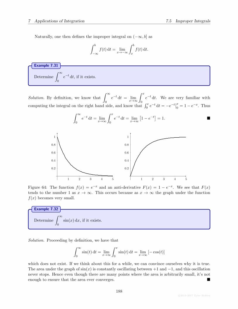
7 Applications of Integration 7.5 Improper Integrals
Naturally, one then defines the improper integral on (−∞, b] as
∫ b
−∞f(t) dt = lim
x→−∞
∫ b
xf(t) dt.
Example 7.31
Determine
∫ ∞
0e−t dt, if it exists.
Solution. By definition, we know that
∫ ∞
0e−t dt = lim
x→∞
∫ x
0e−t dt. We are very familiar with
computing the integral on the right hand side, and know that∫ x
0 e−t dt = −e−t
∣∣x0
= 1− e−x. Thus
∫ ∞
0e−t dt = lim
x→∞
∫ x
0e−t dt = lim
x→∞
[1− e−t
]= 1. �
1 2 3 4 5
0.2
0.4
0.6
0.8
1
1 2 3 4 5
0.2
0.4
0.6
0.8
1
Figure 64: The function f(x) = e−x and an anti-derivative F (x) = 1 − e−x. We see that F (x)tends to the number 1 as x → ∞. This occurs because as x → ∞ the graph under the functionf(x) becomes very small.
Example 7.32
Determine
∫ ∞
0sin(x) dx, if it exists.
Solution. Proceeding by definition, we have that
∫ ∞
0sin(t) dt = lim
x→∞
∫ x
0sin(t) dt = lim
x→∞[− cos(t)]
which does not exist. If we think about this for a while, we can convince ourselves why it is true.The area under the graph of sin(x) is constantly oscillating between +1 and −1, and this oscillationnever stops. Hence even though there are many points where the area is arbitrarily small, it’s notenough to ensure that the area ever converges. �
188c©2013-2017 Tyler Holden
7.5 Improper Integrals 7 Applications of Integration
Intuitively, it seems like functions which tend to zero may have a convergent improper integral.However, this is not always the case. It is necessary that function goes to zero ’fast enough’ toensure that the area is positive.
Proposition 7.33
If a > 0 is an arbitrary positive number, then
∫ ∞
a
1
xpdx converges if and only if p > 1.
Proof. If p = 1 then ∫ ∞
a
1
tdt = lim
x→∞log(x/a) =∞
so the integral diverges. Thus assume that p 6= 1, for which we have
∫ ∞
a
1
tpdt = lim
x→∞
[1
1− p1
xp−1
]x
a
.
We know that 1/xp−1 converges only if and if the power is non-negative; that is, p − 1 ≥ 0.Combining this with p 6= 1 tells us that the improper integral converges if and only if p > 1.
As was computed explicitly, this implies that
∫ ∞
1
1
xdoes not converge, which is a result that
often confuses students.
What happens if we want to define the improper integral on (−∞,∞)?
Definition 7.34
If f is integrable on every interval [a, b] ⊆ R, then we say that
∫ ∞
−∞f(t) dt converges if, for
any c ∈ R we have both
∫ c
−∞f(t) dt converges, and
∫ ∞
cf(t) dt converges.
In this case, we seta ∫ ∞
−∞f(t) dt =
∫ c
−∞f(t) dt+
∫ ∞
cf(t) dt.
aThe student should convince him/herself that the value of the improper integral does not depend on thevalue of c.
This is very different than simply demanding that
∫ ∞
−∞f(t) dt = lim
x→∞
∫ x
−xf(t) dt exists.
c©2013-2017 Tyler Holden
189
7 Applications of Integration 7.5 Improper Integrals
The reason is that the value of the integral should not depend on ’how quickly’ we take our limits.For example
limx→∞
∫ x
−xsin(t) dt = lim
x→∞[cos(−x)− cos(x)] = 0
since cosine is an even function. On the other hand,
limx→∞
∫ 2x
−xsin(t) dt = lim
x→∞[cos(−x)− cos(2x)] does not exist.
Example 7.35
Determine
∫ ∞
−∞e−|t| dt.
Solution. A natural place to split our interval will be at 0. Now
∫ ∞
0e−|t| dt =
∫ ∞
0e−t dt since t > 0
= 1 by Example 7.31.
Similarly,
∫ 0
−∞e−|t| dt = 1, thus
∫ ∞
−∞e−|t| dt =
∫ 0
−∞e−|t| dt+
∫ ∞
0e−|t| dt = 2. �
7.5.2 Unbounded Functions
The case of unbounded functions often poses even more difficulty, since it is very tempting to justblindly apply the Fundamental Theorem of Calculus without paying attention.
Example 7.36
Compute the integral
∫ 1
−1
1
x2dx.
Solution. We know that the anti-derivative of 1x2
is − 1x , so if we were to just blindly apply the FTC
we would get ∫ 1
−1
1
x2dx = −1
x
∣∣∣1
−1= −2.
Unfortunately, this is completely and totally wrong. Our first hint at a miscalculation isprobably the fact that 1
x2is everywhere positive, yet we somehow ended up with a negative integral.
190c©2013-2017 Tyler Holden
7.5 Improper Integrals 7 Applications of Integration
In fact, the integral is infinite. To see this, note that since 1x2> 0 then
∫ 1
−1
1
x2dx ≥
∫ 1
ε
1
x2dx
= −1
x
∣∣∣1
ε
=1
ε− 1,
and that by choosing ε to be small enough we can make the integral arbitrarily large. The reason isthat the function 1
x2is not integrable on the interval [−1, 1] (all integrable functions are bounded!),
and hence we could not apply the FTC. �
Exercise: Compare the following two expressions:
limε→0+
[∫ −ε
−1
1
xdx+
∫ 1
ε
1
xdx
]limε→0+
[∫ −ε
−1
1
xdx+
∫ 1
2ε
1
xdx
]
The way to deal with unbounded functions is precisely the same way that we deal with un-bounded intervals: we take a limit.
Definition 7.37
If f is a function on [a, b], unbounded at a, but integrable on [x, b] for every x > a then wedefine the improper integral
∫ b
af(t) dt = lim
x→a+
∫ b
xf(t) dt.
If this limit is finite we say that the improper integral converges; otherwise, we say that theimproper integral diverges.
Similarly, if f were unbounded at b, we would define the improper integral as∫ b
af(t) dt = lim
x→b−
∫ x
af(t) dt.
Example 7.38
Evaluate
∫ 5
3
t√t2 − 9
dt, if it exists.
Solution. We immediately recognize that there could be a problem at t = 3. Using the substitutionu = t2 − 9 we get
∫ 5
3
t√t2 − 9
dt = limx→3+
[√t2 − 9
]5
x
= limx→3+
[4−
√x2 − 9
]= 4. �
c©2013-2017 Tyler Holden
191
7 Applications of Integration 7.5 Improper Integrals
Just as in the case of integrating from (−∞,∞) we must also be careful about integrating onboth sides of an unbounded function.
Definition 7.39
If f is a function on [a, b] which is unbounded at c ∈ [a, b] then we say that the improperintegral
∫ b
af(t) dt converges, if and only if
∫ c
af(t) dt and
∫ b
cf(t) dt both exist.
In this case, we set ∫ b
af(t) dt =
∫ c
af(t) dt+
∫ b
cf(t) dt.
Proposition 7.40
For any a 6= 0 we have that
∫ a
0
1
tpdt converges, if and only if p < 1.
Proof. For simplicity, let’s assume that a > 0. If p = 1 then
∫ a
0
1
tdt = lim
x→0+
∫ a
x
1
tdt = lim
x→0+log(t)
∣∣∣∣a
x
=∞.
If p 6= 1 then ∫ 1
0
1
tpdt = lim
x→0+
∫ a
x
1
tdt =
1
1− p limx→0+
1
xp−1
∣∣∣∣a
x
.
The limit converges if and only if p− 1 ≤ 0 so that p ≤ 1. Combined with the fact that p 6= 1 weget p < 1 as required.
7.5.3 The Basic Comparison Test
In this section, we develop some techniques to make our lives simpler in terms of dealing improperintegrals. The idea is something like the following: Say that you were asked to determine whetherthe following improper integral converged:
∫ ∞
0
[2 + sin(x)
x
]dx,
or how about ∫ ∞
1
x2 + 1
x4 + 3x2 − 4x+ 1dx?
Neither of these integrals are easy to compute explicitly; in fact, sin(x)x cannot be solved in terms of
elementary functions, but appears often enough to have a name: The Sine Integral. The goal, as isoften the case with mathematics, is to reformulate these problems into ones that are much easier
192c©2013-2017 Tyler Holden
7.5 Improper Integrals 7 Applications of Integration
to solve, or that have already been solved. The Basic Comparison Test is the simplest of the basictests, and exploits the “monotonicity” of the integral. In particular, the following lemma is ratherintuitive:
Theorem 7.41: The Basic Comparison Test for Improper Integrals
Let f(x), g(x) be functions on an interval [a,∞) such that 0 ≤ f(x) ≤ g(x) for all x ∈ [a,∞).
1. If
∫ ∞
ag(t) dt converges then
∫ ∞
af(t) dt converges.
2. If
∫ ∞
af(t) dt diverges then
∫ ∞
ag(t) dt diverges.
The idea is again a type of ‘Squeeze Theorem’ argument. If the integral of the bigger function gbecomes finite, the monotonicity of the integral cannot allow f to go off to infinity. Similarly, if theintegral of the smaller function f goes off to infinity, the larger function’s integral must also diverge.A good question at this point is to ask whether any of the integrals could oscillate and hence notconverge. The condition that 0 ≤ f(x) ≤ g(x) guarantees that the integrands are positive: thismeans that the corresponding integrals are increasing functions.
Example 7.42
Show that
∫ ∞
1
2 + sin(x)
xdx diverges.
Solution. We want to compare the function 2+sin(x)x to some function which we know diverges. The
idea to keep in mind is that in the limit as x → ∞, the sin(x) term does not play a significantrole; rather, the x-term in the denominator dominates. This suggests that we make the comparisonagainst 1
x . Indeed, notice that since −1 ≤ sin(x) ≤ 1 for all x, we have
2 + sin(x)
x≥ 1
x.
By Proposition 7.40, we know that∫∞
11x diverges, so by the comparison test it follows that
∫ ∞
1
2 + sin(x)
xdx diverges. �
Example 7.43
Determine whether
∫ ∞
0
x√x6 + 1
dx converges or diverges.
Solution. Once again, we just want to look at which terms in the numerator and denominatordominate in the limit x→∞. Certainly, we do not expect x6 + 1 to be too much different than x6
for very large x, so we will compare our integrand to the function
x√x6
=1
x2.
c©2013-2017 Tyler Holden
193

7 Applications of Integration 7.5 Improper Integrals
Indeed, since 1 + x6 ≥ x6 we have that 1√x6≥ 1√
1+x6, which in turn implies that
1
x2=
1√x6≥ x√
x6 + 1.
Now the integral of the left-hand-side converges by 7.40, so by the Comparison Test we know that∫ ∞
0
x√x6 + 1
dx converges. �
7.5.4 The Limit Comparison Test
The Basic Comparison Test is just that, basic. Often times the obvious inequality that you wantactually ends up going in the wrong direction, yet the integrals are so similar that you feel like youshould still be able to compare them. Example 7.45 below will demonstrate precisely this.
The Limit Comparison Test will fix this by asking the question: “Do f and g grow at roughlythe same rate?”
Theorem 7.44: The Limit Comparison Test
Let f, g be integrable functions on all subintervals of [a,∞) and satisfy 0 ≤ f(x) ≤ g(x). If
0 < limx→∞
f(x)
g(x)<∞
then
∫ ∞
af(x) dx converges if and only if
∫ ∞
ag(x) dx converges.
The statement that f(x)g(x) converges to some finite, non-zero number, means that f and g grow
asymptotically at the same speed, up to some multiplicative constant (which is precisely the valueof the limit). Note that if the limit is 0, eventually one must have g(x) ≥ f(x) and can use theBasic Comparison Test appropriately. Similarly, if the limit is ∞, then eventually f(x) ≥ g(x) andagain the Basic Comparison Test can be used.
Also notice that the ratio does not matter, for if f(x)g(x) → L which is finite and positive, then
g(x)f(x) → 1
L which is also finite and positive.
Example 7.45
Determine whether
∫ ∞
1
1√1 + x
dx converges or diverges.
Solution. If one were to try to use the Basic Comparison Test, the obvious inequality is that1√1+x≤ 1√
x. But this does not tell us anything! The right-hand-side diverges, and so does not
impose its will on the left-hand-side. Instead, we recognize that
limx→∞
√x√
1 + x= 1.
194c©2013-2017 Tyler Holden
8 Sequences and Series
Thus by the Limit Comparison Test, since∫∞
11√x
dx diverges, we necessarily have that∫∞
11√1+x
dx
diverges as well. �
Example 7.46
Determine whether
∫ ∞
1
x2 + 1
x4 + 3x2 − 4x+ 1dx converges or diverges.
Solution. With a strong enough argument, one might be able to argue this example using the BasicComparison Test, but the Limit Comparison Test proves much simpler. Again the idea is to lookat how the numerator and denominator grow asymptotically. The numerator grows as x2, whilethe denominator grows as x4, meaning that the combined system grows as 1/x2. To invoke theLimit comparison Test, we must compute the limit of the ratio of these functions:
limx→∞
x2 + 1
x4 + 3x2 − 4x+ 1
1
1/x2= lim
x→∞
x4 + x2
x4 + 3x2 − 4x+ 1= 1.
Since∫∞
11x2
dx converges (by Proposition 7.40), we conclude by the Limit Comparison Test that
∫ ∞
1
x2 + 1
x4 + 3x2 − 4x+ 1dx also converges. �
8 Sequences and Series
The remainder of this text will seem tangential to that which came before, but exists in thesame vein. In particular, our focus digresses from objects on the continuum, like functions of realnumbers, and instead concentrates on discrete objects. We will draw the appropriate analogiesbetween differential/integral calculus as we progress.
8.1 Sequences
8.1.1 Definition
An infinite sequence in R is any ordered collection of real numbers. Alternatively, a sequence isany function a(n) which has domain N and outputs a real number. For example, the functiona(n) = 1/n is such a sequence, and we have
a(1) = 1, a(2) =1
2, a(3) =
1
3, a(4) =
1
4, . . . .
Notationally, we often write
a1 = 1, a2 =1
2, a3 =
1
3, a4 =
1
4, . . . ,
with a general element of the sequence written as an = a(n). When we wish to refer to the entiresequence, and not just a particular element, we write (an)∞n=1. On occasion we will abuse thisnotation, and conflate an with (an)∞n=1.
c©2013-2017 Tyler Holden
195
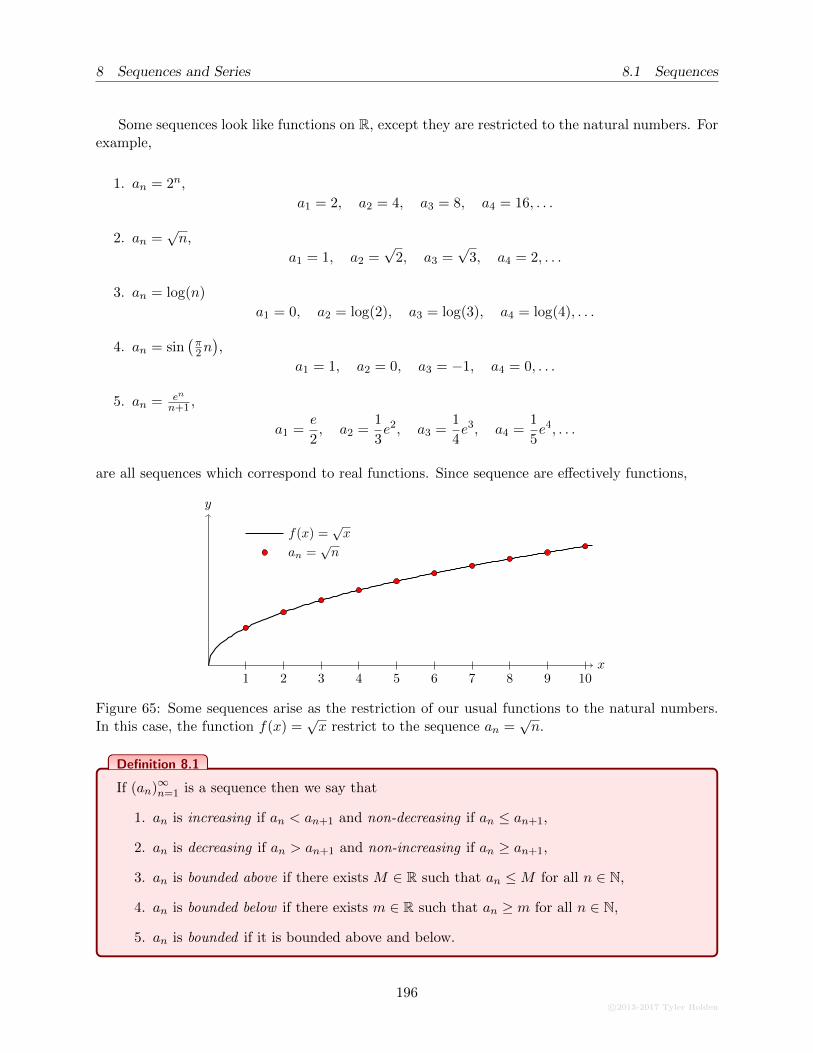
8 Sequences and Series 8.1 Sequences
Some sequences look like functions on R, except they are restricted to the natural numbers. Forexample,
1. an = 2n,
a1 = 2, a2 = 4, a3 = 8, a4 = 16, . . .
2. an =√n,
a1 = 1, a2 =√
2, a3 =√
3, a4 = 2, . . .
3. an = log(n)
a1 = 0, a2 = log(2), a3 = log(3), a4 = log(4), . . .
4. an = sin(π2n),
a1 = 1, a2 = 0, a3 = −1, a4 = 0, . . .
5. an = en
n+1 ,
a1 =e
2, a2 =
1
3e2, a3 =
1
4e3, a4 =
1
5e4, . . .
are all sequences which correspond to real functions. Since sequence are effectively functions,
x
y
1 2 3 4 5 6 7 8 9 10
f(x) =√x
an =√n
Figure 65: Some sequences arise as the restriction of our usual functions to the natural numbers.In this case, the function f(x) =
√x restrict to the sequence an =
√n.
Definition 8.1
If (an)∞n=1 is a sequence then we say that
1. an is increasing if an < an+1 and non-decreasing if an ≤ an+1,
2. an is decreasing if an > an+1 and non-increasing if an ≥ an+1,
3. an is bounded above if there exists M ∈ R such that an ≤M for all n ∈ N,
4. an is bounded below if there exists m ∈ R such that an ≥ m for all n ∈ N,
5. an is bounded if it is bounded above and below.
196c©2013-2017 Tyler Holden
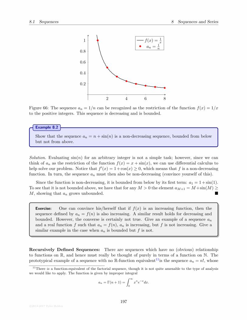
8.1 Sequences 8 Sequences and Series
2 4 6 8
0.2
0.4
0.6
0.8
1 f(x) = 1x
an = 1n
Figure 66: The sequence an = 1/n can be recognized as the restriction of the function f(x) = 1/xto the positive integers. This sequence is decreasing and is bounded.
Example 8.2
Show that the sequence an = n+ sin(n) is a non-decreasing sequence, bounded from belowbut not from above.
Solution. Evaluating sin(n) for an arbitrary integer is not a simple task; however, since we canthink of an as the restriction of the function f(x) = x+ sin(x), we can use differential calculus tohelp solve our problem. Notice that f ′(x) = 1+cos(x) ≥ 0, which means that f is a non-decreasingfunction. In turn, the sequence an must then also be non-decreasing (convince yourself of this).
Since the function is non-decreasing, it is bounded from below by its first term: a1 = 1 + sin(1).To see that it is not bounded above, we have that for any M > 0 the element aM+1 = M+sin(M) ≥M , showing that an grows unbounded. �
Exercise: One can convince his/herself that if f(x) is an increasing function, then thesequence defined by an = f(n) is also increasing. A similar result holds for decreasing andbounded. However, the converse is certainly not true. Give an example of a sequence anand a real function f such that an = f(n), an is increasing, but f is not increasing. Give asimilar example in the case when an is bounded but f is not.
Recursively Defined Sequences: There are sequences which have no (obvious) relationshipto functions on R, and hence must really be thought of purely in terms of a function on N. Theprototypical example of a sequence with no R-function equivalent11is the sequence an = n!, whose
11There is a function-equivalent of the factorial sequence, though it is not quite amenable to the type of analysiswe would like to apply. The function is given by improper integral
an = Γ(n+ 1) =
∫ ∞0
xne−xdx.
c©2013-2017 Tyler Holden
197
8 Sequences and Series 8.1 Sequences
first few terms are given by
a1 = 1, a2 = 2, a3 = 6, a4 = 24, a5 = 120, a6 = 720, a7 = 5040, . . . .
Another class of example are those functions which are defined recursively. For example, defininga1 = 1 and setting an =
√an−1 + 1 yields the sequence12
a1 = 1, a2 =√
2, a3 =
√√2 + 1, a4 =
√√√2 + 1 + 1, . . .
or equivalently
a1 =√
1, a2 =
√1 +√
1, a3 =
√1 +
√1 +√
1, a4 =
√
1 +
√1 +
√1 +√
1, . . .
A rather famous example is given by the Fibonacci sequence. Define a0 = a1 = 1 and setan = an−1 + an−2 for n ≥ 2. The first few terms of this sequence are given by13
1, 1, 2, 3, 5, 8, 13, 21, 34, 55, 89, . . . .
We will not concern ourselves too much with recursively defined sequences, but it is worthnoting that they exist and are an interesting area of study in their own right.
8.1.2 Limits of Sequences
Treating sequences as functions, and especially realizing the analogy of a sequence to a function onR, allows us to talk about the notion of convergence of a sequence. Roughly speaking, we will saythat a sequence converges if it behaves as though the function a(n) has a horizontal asymptote. Ifwe have this idea in our mind, we can immediately adapt the notion of a horizontal asymptote forreal functions to sequences:
Definition 8.3
A sequence an is said to converge to a limit L ∈ R if, by taking n sufficiently large, we canmake an arbitrarily close to L. In this case we write
limn→∞
an = L, or (an)n→∞−−−→ L.
If no such L exists, we say that the sequence diverges.
For example, the sequence an = 1/n converges. As n becomes very large, 1/n becomes verysmall, so the limit is
limn→∞
an = limn→∞
1
n= 0.
12This is a very important example of a recursive sequence. To see why, consider Exercise 8.1.313Again, there is a real function which defines this sequence: If ϕ± = 1
2
(1±√
5)
then the function F defined on[1,∞) given by F (x) = 1√
5[ϕx+ − ϕx−] restricts to the Fibonacci sequence.
198c©2013-2017 Tyler Holden
8.1 Sequences 8 Sequences and Series
On the other hand, the sequence an = sin(π2n) diverges, since
a1 = 1, a2 = 0, a3 = −1, a4 = 0, a5 = 1, . . .
continues in this pattern forever, failing to approach any one particular number. The sequencean = n2 also does not converge, since
a1 = 1, a2 = 4, a3 = 9, a4 = 16, a5 = 25, . . .
grows unbounded.
The previous two sequences demonstrate that a sequence can fail to converge in two differentways. The sequence an = sin
(π2n)
failed to converge because because it simply did not approachany number, while an = n2 went off to infinity. In this latter case, we will sometimes write
limn→∞
an =∞ or (an)→∞.
This does not mean that the sequence converges, we are merely specifying the precise nature withwhich the sequence diverges.
Notice that an = 1/n converges to zero, just as the function f(x) = 1/x did. This behaviourgeneralizes quite nicely.
Theorem 8.4
Let f(x) be a function on R and define a sequence an = f(n).
If limn→∞
f(x) = L then limn→∞
an = L.
Many of the Limit Laws we saw in Theorem 2.6 hold for sequences as well:
Theorem 8.5: Limit Laws for Sequences
Let (an)→ L and (bn)→M be convergent sequences and c ∈ R be a constant.
1. The sequence (an + bn) is convergent and (an + bn)→ L+M ,
2. The sequence (anbn) is convergent and (anbn)→ LM ,
3. The sequence (can) is convergent and (can)→ cL,
4. If M 6= 0 then the sequence (an/bn) converges and (an/bn)→ L/M .
Example 8.6
Show that the sequence an =n2 + 1
2n2 − 7n+ 3converges, and determine its limit.
Solution. We can proceed in precisely the same manner we would for functions on R. As the n2
term grows fastest in the limit n→∞, we renormalize by dividing the numerator and denominator
c©2013-2017 Tyler Holden
199

8 Sequences and Series 8.1 Sequences
by this factor.
limn→∞
n2 + 1
2n2 − 7n+ 3= lim
n→∞
n2 + 1
2n2 − 7n+ 3
1/n2
1/n2
= limn→∞
1 + 1/n2
2 + 7/n+ 3/n2
=1
2. �
Example 8.7
Show that the sequence an =en + e−n
4en − 3n2converges and determine its corresponding limit.
Solution. The term which grows fastest is en, so we normalize by this term to get
limn→∞
en + e−n
4en − 3n2= lim
n→∞
en + e−n
4en − 3n2
e−n
e−n
= limn→∞
1 + e−2n
4− 3e−nn2
=1
4.
Here the student should check that e−nn2 n→∞−−−→ 0. �
Example 8.8
Determine whether the sequence an =1− n3
n2 + 3n+ 1converges.
Solution. The term which grows fastest is n3, so normalizing gives
limn→∞
1− n3
n2 + 3n+ 1= lim
n→∞
1− n3
n2 + 3n+ 1
1/n3
1/n3
= limn→∞
1/n3 − 1
1/n+ 3/n2 + 1/n3.
In the limit as n → ∞ our numerator converges to 1, while our denominator converges to 0. Thecombination of these two things tells us that our sequence diverges. In fact, for large n notice thatthe numerator is negative and the denominator is positive, so
limn→∞
1− n3
n2 + 3n+ 1= −∞. �
Example 8.9
Determine whether the sequence an = n[2 + cos(n)] converges.
200c©2013-2017 Tyler Holden
8.1 Sequences 8 Sequences and Series
Solution. We claim that this sequence does not converge. Indeed, since 2 + cos(n) ≥ 1 for all n wehave that
|an| = |n[2 + cos(n)]| ≥ |n|.which means an cannot possibly be bounded, either above or below. Hence (an)∞n=1 is divergent. �
8.1.3 Theorems on Convergent Sequences
Theorem 8.10: Squeeze Theorem for Sequences
Assume that for sufficiently large k we have an ≤ bn ≤ cn. If (an)→ L and (cn)→ L, then(bn) is also convergent with limit L.
Example 8.11
Show that the sequence an = (−1)n/n2 converges and determine its limit.
Solution. In absolute value, we have
0 ≤ an ≤ |an| =∣∣∣∣(−1)n
n2
∣∣∣∣ =1
n2.
Setting an = 0 and cn = 1/n2, both sequences converge to 0. By the Squeeze Theorem, we concludethat
limn→∞
bn = limn→∞
(−1)n
n2= 0. �
Example 8.12
Show that the sequence an = sin(n)/n converges.
Solution. Since | sin(n)| ≤ 1 for all n, we have
− 1
n≤ sin(n)
n≤ 1
n.
Setting an = −1/n and cn = 1/n, both limits converge to 0. By the Squeeze Theorem,
limn→∞
sin(n)
n= 0. �
There are a plethora of ways of defining continuous functions, and now we have the tools tointroduce yet another.
Theorem 8.13
A real function f(x) is continuous if and only if whenever an → L then f(an)→ f(L).
c©2013-2017 Tyler Holden
201
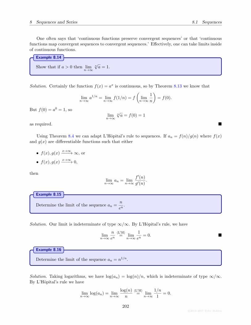
8 Sequences and Series 8.1 Sequences
One often says that ‘continuous functions preserve convergent sequences’ or that ‘continuousfunctions map convergent sequences to convergent sequences.’ Effectively, one can take limits insideof continuous functions.
Example 8.14
Show that if a > 0 then limn→∞
n√a = 1.
Solution. Certainly the function f(x) = ax is continuous, so by Theorem 8.13 we know that
limn→∞
a1/n = limn→∞
f(1/n) = f
(limn→∞
1
n
)= f(0).
But f(0) = a0 = 1, solimn→∞
n√a = f(0) = 1
as required. �
Using Theorem 8.4 we can adapt L’Hopital’s rule to sequences. If an = f(n)/g(n) where f(x)and g(x) are differentiable functions such that either
• f(x), g(x)x→∞−−−→∞, or
• f(x), g(x)x→∞−−−→ 0,
then
limn→∞
an = limn→∞
f ′(n)
g′(n).
Example 8.15
Determine the limit of the sequence an =n
en.
Solution. Our limit is indeterminate of type ∞/∞. By L’Hopital’s rule, we have
limn→∞
n
en〈L′H〉
= limn→∞
1
en= 0. �
Example 8.16
Determine the limit of the sequence an = n1/n.
Solution. Taking logarithms, we have log(an) = log(n)/n, which is indeterminate of type ∞/∞.By L’Hopital’s rule we have
limn→∞
log(an) = limn→∞
log(n)
n
〈L′H〉= lim
n→∞
1/n
1= 0.
202c©2013-2017 Tyler Holden
8.1 Sequences 8 Sequences and Series
This tells us that log(an)→ 0, but we want the limit of an. Appealing to Theorem 8.13 we have
limn→∞
an = limn→∞
exp(log(an)) = exp(
limn→∞
log(an))
= exp(0) = 1. �
Theorem 8.17
Every convergent sequence is bounded.
The converse of Theorem 8.17 is not true, for the function an = (−1)n is bounded but notconvergent. The problem is that an is allowed to oscillate. We can get a partial converse by addingthe additional criterion that the sequence is either increasing or decreasing.
Theorem 8.18: Monotone Convergence Theorem
If (an) is bounded from above and non-decreasing, then (an) is convergent.
Exercise: Using the Monotone Convergence Theorem, can you show that if (an) is boundedfrom below and non-increasing then (an) is convergent?
Example 8.19
Determine whether the sequence an =2n
n!is convergent.
Solution. We havean+1
an=
2n+1
(n+ 1)!
n!
2n=
2
n+ 1,
so that if n ≥ 2 we have an+1 < an and the sequence is decreasing. It is easy to see that an isalways positive, and so by the Monotone Convergence Theorem we know that (an) converges. �
Example 8.20
Consider the sequence defined by a1 = 1 and an+1 =n
2n+ 1an. Determine whether this
limit converges and if so, find the limit.
Solution. We begin by noticing that this sequence is decreasing, since an+1
an= n
2n+1 < 1 whichimplies that an+1 < an. Furthermore, the sequence is bounded below by 0; that is, we claimthat every an is positive. This follows quite quickly by induction, for clearly a1 = 1 > 0 andan+1 = n
2n+1an > 0 by the induction hypothesis. By (Corollary to) the Monotone ConvergenceTheorem, (an) converges, say to L. Now taking the limit as n→∞ of the equation an+1 = n
2n+1anwe get
L =1
2L
for which the only possible real value of L is L = 0. �
c©2013-2017 Tyler Holden
203
8 Sequences and Series 8.2 Infinite Series
Exercise: Consider the sequence a1 = 1 and an =√
1 + an−1. Show that this sequence isincreasing and bounded from above. Conclude that it converges. Show that the limit of this
sequence is L = 1+√
52 : the golden ratio.
8.2 Infinite Series
8.2.1 Definition
Section 5.1 introduced sigma notation as a convenient way of writing down finite sums; namely,
n∑
i=m
ai = am + am+1 + · · ·+ an−1 + an.
The summand here conveniently looks like a sequence, though with finitely many terms. In fact,we will be extending the notion of the finite sum above to an infinite sum, called an infinite series.
Definition 8.21
Let (an)∞n=1 be a sequence. Define the nth partial sum of (an) to be
Sn =
n∑
k=1
ak.
We say that the infinite series
∞∑
n=1
an converges if the sequence (Sn)∞n=1 converges as a se-
quence, and we set∞∑
n=1
an = limn→∞
Sn.
We say that the infinite series diverges otherwise.
Notice that Sn = Sn−1 + an. For example, if we let an = 1n , then our first few partial sums are
given by
S1 = 1 S2 = S1 +1
2= 1 +
1
2=
3
2
S3 = S2 +1
3=
11
6S4 = S3 +
1
4=
25
12
S5 = S4 +1
5=
137
60S6 = S5 +
1
6=
49
20.
It is not at all clear from looking at the partial sums whether or not this sequence converges.Shortly, we will study techniques that will allow us to determine whether series converge (thoughwe will rarely be able to determine the limit to which the series converges).
Here is an important distinction to make, as students often confuse sequences and series:
204c©2013-2017 Tyler Holden
8.2 Infinite Series 8 Sequences and Series
• A sequence is a collection of elements (an)∞n=1. Note that an need not be in any way relatedto an−1. The analogy to keep in mind that is sequences behave like functions.
• A series is a sum of elements of a sequence, with the partial sums being related via Sn =Sn−1 + an. The analogy to keep in mind is that a sum is like an improper integral of afunction.
This analogy between sequences/series and functions/integrals is an important one to keep in mind.
Since the convergence of a series is defined in terms of the limits of its partial sums (a sequence),the limit laws for sequences immediately give us the following result:
Theorem 8.22
Let
∞∑
k=1
an and
∞∑
k=1
bn be convergent series.
1. The sum of the series is convergent and
∞∑
k=1
(an + bn) =∞∑
k=1
an +∞∑
k=1
bn.
2. For any c > 0, we have∞∑
k=1
(can) = c
∞∑
k=0
an.
Proof. Let (sn)→ L be the partial sums of∑∞
k=1 an and (tn)→M be the partial sums for∑∞
k=1 bn.The partial sum of the sum is given by
un =∞∑
k=1
(an + bn) =∑
k=1
an +∑
k=1
bn = sn + tn.
By Theorem 8.5, we have (un) = (sn + tn)→ L+M , and so
∞∑
k=1
(an + bn) =∞∑
k=1
an +∞∑
k=1
bn.
The proof for (2) is similar.
8.2.2 Some Special Series
Geometric Series: A geometric series is a series defined by a sequence (an) where an = ran−1
for some r ∈ R. For example,
a0 = 1, a1 =1
2, a2 =
1
4, a3 =
1
8, a4 =
1
16, . . .
c©2013-2017 Tyler Holden
205
8 Sequences and Series 8.2 Infinite Series
satisfies the relation an = 12an−1. We can write such series as
∞∑
k=0
ark,
where a = a1 and r = an/an−1 for any n.
Theorem 8.23
For any |r| < 1 we have∞∑
k=0
rk =1
1− r (8.1)
and the series diverges otherwise.
Proof. The partial sums are given by Sn = 1 + r + r2 + · · ·+ rn. Multiplying by 1− r we get
(1− r)Sn = 1 + r + r2 + r3 + r4 + · · ·+ rn
− r − r2 − r3 − r4 + · · · − rn − rn+1
= 1− rn+1.
Solving for Sn gives sn =1− rn+1
1− r . Since |r| < 1, we have that rn+1 n→∞−−−→ 0, so
∞∑
k=0
rk = limn→∞
Sn = limn→∞
1− rn−1
1− r =1
1− r .
An interesting if non-rigorous argument that proves the same result is to see that
(1− r)(1 + r + r2 + r3 + · · · ) = 1 + r + r2 + r3 + · · ·− r − r2 − r3 − · · ·
= 1.
In an entirely formal sense (that is, treating r purely as a symbol without assigning it any value)we see that (1 − r) is the multiplicative inverse of (1 + r + r2 + · · · ), giving the desired results aswell. Determining from this which values of r actually make sense is something that we will see ina later chapter.
Example 8.24
Determine the limit
∞∑
k=2
1
2k.
Solution. Notice that our summation index begins at 2, and not 0 as in (8.1). We can fix this byrealizing that
∞∑
k=2
1
2k=
∞∑
k=0
1
2k− 1− 1
2=
1
1− 1/2− 1− 1
2= 2− 1− 1
2=
1
2. �
206c©2013-2017 Tyler Holden
8.2 Infinite Series 8 Sequences and Series
Example 8.25
Determine the value of the series∞∑
n=0
(−2)n
en.
Solution. Here our ratio is r = −2/e. Since e ≈ 2.7182 we know |r| < 1. By (8.1) we have
∞∑
n=0
(−2)n
en=
1
1− (−2/e)=
e
e+ 2. �
Example 8.26
Determine the value of the series
∞∑
k=10
−3
4k.
Solution. The −3 can be pulled outside of the sum. As our index does not start at 0 we couldsubtract the first 10 terms, but this is rather onerous. Instead, realize that by writing
∞∑
k=10
1
4k=
1
410+
1
411+
1
412+
1
413+ · · ·
=1
410
(1
4+
1
42+
1
43+ · · ·
)
=1
410
∞∑
k=0
1
4k.
Putting this all together we get
∞∑
k=10
−3
4k=−3
410
∞∑
k=0
1
4k=−3
410
1
1− 1/3= − 9
2 · 410= − 9
221. �
Telescoping Series: Telescoping series are ones in which many of the internal summands cancelone another out. For example, a telescoping sum arises when we consider the Riemann sum of aconstant function. If f(x) = c and we partition [a, b] into n equal subintervals [xi, xi+1], then theRiemann sum is
L(f) =n∑
i=1
f(xi)(xi − xi−1) = cn∑
i=1
(xi − xi−1).
Notice what happens if we expand out a few terms of the sum: we get
(x1 − x0) + (x2 − x1) + (x3 − x2) + · · ·+ (xn−1 − xn−2) + (xn − xn−1).
For that majority of terms, both xi and −xi appear in the summation and hence cancel one anotherout. The only terms which survive are the first and last, so that the sum reduces to xn − x0.
Uf (P ) = c(xn − x0) = c(b− a)
c©2013-2017 Tyler Holden
207
8 Sequences and Series 8.3 Convergence Tests
exactly as expected.
Example 8.27
Determine the value of the series∞∑
k=1
1
k(k + 1)if it converges.
Solution. The trick is to realize our sum as a telescoping series. Using partial fractions, we get that
1
k(k + 1)=
1
k− 1
k + 1
so that the nth partial fraction is given by
Sn =n∑
k=1
1
k(k + 1)=∞∑
k=1
[1
k− 1
k + 1
]
=
(1− 1
2
)+
(1
2− 1
3
)+
(1
3− 1
4
)+ · · ·+
(1
n− 1− 1
n
)+
(1
n− 1
n+ 1
)
= 1− 1
n+ 1=
n
n+ 1.
We now take the limit as n→∞ and we find that
∞∑
k=1
1
k(k + 1)= lim
n→∞
n∑
k=1
1
k(k + 1)= lim
k→∞
k
k + 1= 1. �
8.3 Convergence Tests
The analogy between infinite series and improper integrals continues in this section with the in-troduction of the basic and limit comparison test. Later, we will develop several more tests whichallow us to infer convergence of infinite series.
Our first result really tests divergence rather than convergence. Intuitively, one should expectthat we require (an) → 0 to even have a chance for the infinite series to converge. Otherwise, if(an)→ L 6= 0 then the infinite series would effectively be ‘adding L to itself infinitely many times,’which would certainly yield a non-finite number. The following is the more precise way of sayingthis:
Theorem 8.28
If
∞∑
k=1
ak converges, then (ak)→ 0.
The contrapositive of this is exactly what we mentioned above: “If (ak) 6→ 0 then∑∞
k=1 akdoes not converge.” However, the converse of Theorem 8.28 is not true. We do not yet have the
208c©2013-2017 Tyler Holden
8.3 Convergence Tests 8 Sequences and Series
techniques to show that this is the case, but the series
∞∑
k=1
1
kdoes not converge,
despite the fact that 1/kk→∞−−−→ 0.
Example 8.29
Show that the series
∞∑
k=0
sin
(πk
2
)diverges.
Solution. Setting ak = sin(πk2
), we know that ak alternates between the values {0,±1} and fails
to converge at all, let alone 0. By Theorem 8.28 we conclude that
∞∑
k=0
sin
(πk
2
)diverges. �
Example 8.30
Determine whether the sequence
∞∑
k=0
k2
k2 + 1converges.
Solution. Setting ak = k2/(k2 + 1) we see that
limk→∞
ak = limk→∞
k2
k2 + 1= 1.
Since this limit is not zero, the series cannot possibly converge, by Theorem 8.28. �
8.3.1 The Integral Test
This tests takes our series/integral analogy to the next level, but allowing us to directly comparethem.
Theorem 8.31: The Integral Test
If f is a continuous, non-negative, decreasing function on [1,∞) then
∞∑
k=1
f(k) converges ⇔∫ ∞
1f(x) dx converges.
The idea here is by appropriate choosing our Riemann sums, we can bound the series by theintegrals. This is shown in Figure 67.
c©2013-2017 Tyler Holden
209
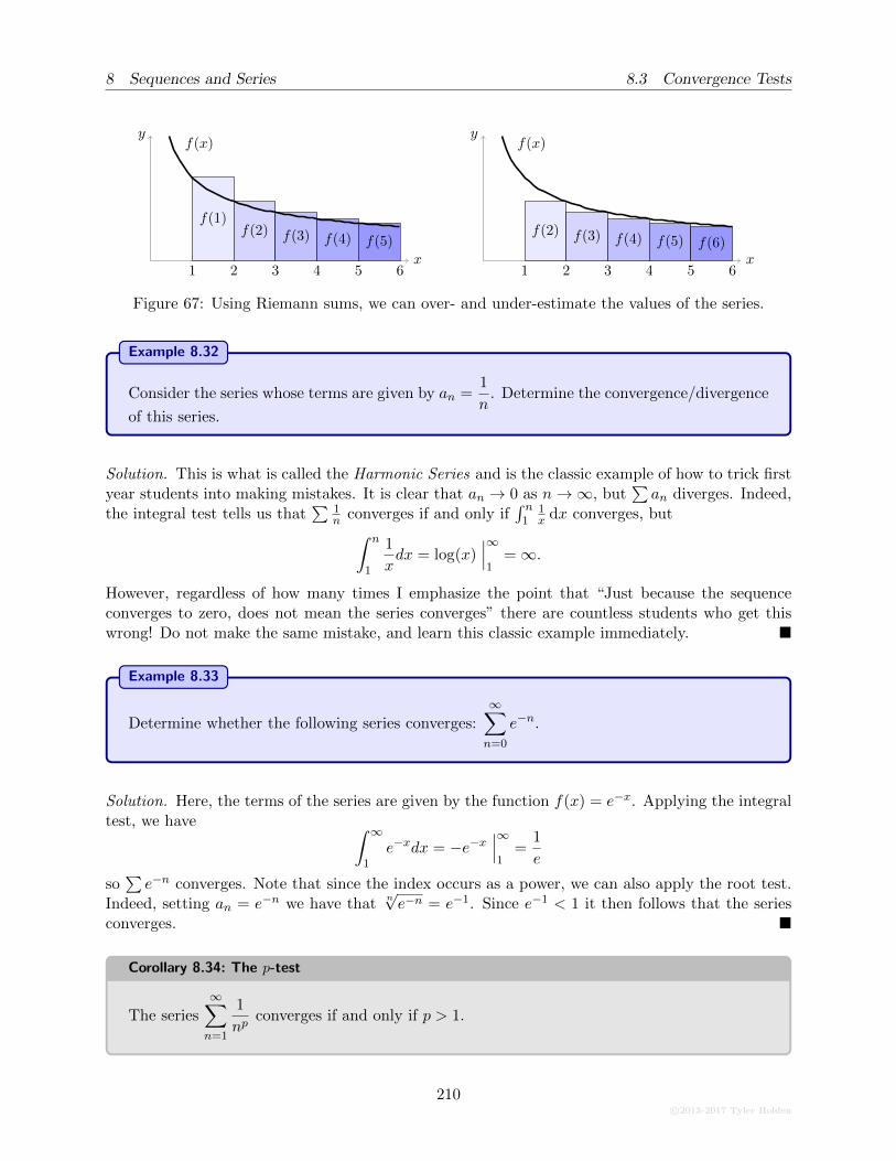
8 Sequences and Series 8.3 Convergence Tests
x
y
1
f(1)
2
f(2)
3
f(3)
4
f(4)
5
f(5)
6
f(x)
x
y
1
f(2)
2
f(3)
3
f(4)
4
f(5)
5
f(6)
6
f(x)
Figure 67: Using Riemann sums, we can over- and under-estimate the values of the series.
Example 8.32
Consider the series whose terms are given by an =1
n. Determine the convergence/divergence
of this series.
Solution. This is what is called the Harmonic Series and is the classic example of how to trick firstyear students into making mistakes. It is clear that an → 0 as n→∞, but
∑an diverges. Indeed,
the integral test tells us that∑ 1
n converges if and only if∫ n
11x dx converges, but
∫ n
1
1
xdx = log(x)
∣∣∣∞
1=∞.
However, regardless of how many times I emphasize the point that “Just because the sequenceconverges to zero, does not mean the series converges” there are countless students who get thiswrong! Do not make the same mistake, and learn this classic example immediately. �
Example 8.33
Determine whether the following series converges:
∞∑
n=0
e−n.
Solution. Here, the terms of the series are given by the function f(x) = e−x. Applying the integraltest, we have ∫ ∞
1e−xdx = −e−x
∣∣∣∞
1=
1
e
so∑e−n converges. Note that since the index occurs as a power, we can also apply the root test.
Indeed, setting an = e−n we have thatn√e−n = e−1. Since e−1 < 1 it then follows that the series
converges. �
Corollary 8.34: The p-test
The series
∞∑
n=1
1
npconverges if and only if p > 1.
210c©2013-2017 Tyler Holden
8.3 Convergence Tests 8 Sequences and Series
Proof. By the Integral Test (Theorem 8.31) and the p-test (Propostion 7.33), we know that
∞∑
k=1
1
npconverges
Theorem 8.31⇔∫ ∞
1
1
xpdx converges
Proposition 7.33⇔ p > 1.
From the p-test we can immediately conclude, for example, that∑∞
k=1 n−2 converges. Note
however that this does not tell us how to determine the value of this series. In fact,
∞∑
k=1
1
n2=π2
6,
but this lies well beyond the scope of these notes.
8.3.2 Comparison Tests
In Section 7.5.3 we saw the Basic Comparison Test (Theorem 7.41) and Limit Comparison Test(Theorem 7.44) for improper integrals. The statement of these tests for series are almost identical.
Theorem 8.35: Basic Comparison Test for Series
Suppose that (an) and (bn) are sequences such that 0 ≤ ak ≤ bk for sufficiently large k.
1. If∑
k bk converges, then∑
k ak converges.
2. If∑
k ak diverges, then∑
k bk diverges.
The idea here is precisely the same as that of Theorem 7.41: If the larger of the two seriesconverges, it forces the smaller sequence to also converge. In the opposite direction, if the smallersequence diverges, then the larger sequence must also diverge.
Example 8.36
Determine whether the series∞∑
n=2
1
n− 1converges or diverges.
Solution. Notice that n > n− 1 so that
1
n≤ 1
n− 1.
The series over the left hand side diverges, as it is the Harmonic Series. By the Basic ComparisonTest (2), we know that
∞∑
n=2
1
n− 1diverges.
�
c©2013-2017 Tyler Holden
211
8 Sequences and Series 8.3 Convergence Tests
Example 8.37
Determine whether∞∑
k=1
1
k3 + k2 + 1converges.
Solution. Note that k2 + 1 ≥ 0 for all k, so k3 + k2 + 1 ≥ k3. Taking reciprocals reverses theinequality, giving
1
k3 + k2 + 1≤ 1
k3.
The series over the right hand side converges by the p-test, so by the Basic Comparison Test (1),
∞∑
k=1
1
k3 + k2 + 1converges. �
Example 8.38
Determine whether the sequence
∞∑
k=1
7n
8n + 2converges.
Solution. By considering the terms which grow fastest in this expression, we suspect that the 2in the denominator should not affect the long term behaviour of the function. We thus have thecomparison
7n
8n + 2≤ 7n
8n=
(7
8
)n.
Now the series∑
k
(78
)nis a geometric series with ratio less than 1, and hence converges. We
conclude by the Basic Comparison Test the∑
k7n
8n+2 converges as well. �
There are very simple circumstances where the Basic Comparison Test fails, when it morallyfeels like it should succeed. For example, consider the simple series
∞∑
n=1
1
2n2 − 1.
It feels like we should be able to compare this to the series∑
1/n2, but when we try to do ouranalysis we get
1
n2≤ 1
n2 − 1.
Since the left hand side converges, the Basic Comparison Test tells us nothing. The key to resolvingthis is the Limit Comparison Test.
212c©2013-2017 Tyler Holden
8.3 Convergence Tests 8 Sequences and Series
Theorem 8.39: Limit Comparison Test for Series
If (an) and (bn) are sequences with positive terms, and limn→∞
akbk
= L for some 0 < L < ∞then ∑
k
ak converges ⇔∑
k
bk converges.
The fact that ak/bk converges to some positive, non-zero number means that ak and bk grow at‘approximately the same speed.’ Hence convergence or divergence of one will immediately implyconvergence/divergence of the other.
Example 8.40
Determine whether the sequence
∞∑
k=0
k10 + 25k7 + 1
k12 − 20converges or diverges.
Solution. We only care about the terms which grow the fastest, so to form our comparison functionwe just consider the biggest factors in each of the numerator and the denominator. Those termsare k10/k12 = 1/k2 and since we know that the series
∑1/k2 converges, it seems likely that so
too will our series above. Indeed, this actually gives us the other series we should use in our LimitComparison Test. Notice that
limk→∞
1k2
k10+25k7+1k12−20
= limk→∞
k12 − 20
k12 + 25k9 + k2
1/k12
1/k12
= limk→∞
1− 20/k12
1 + 251/k2 + 1/k10
= 1.
Thus the Limit Comparison Test tells us that the series converges. �
Example 8.41
Determine whether the series
∞∑
k=1
n+√n
n2 − 3converges or diverges.
Solution. Taking the largest terms in the numerator and denominator, we compare to n/n2 = 1/n.
c©2013-2017 Tyler Holden
213
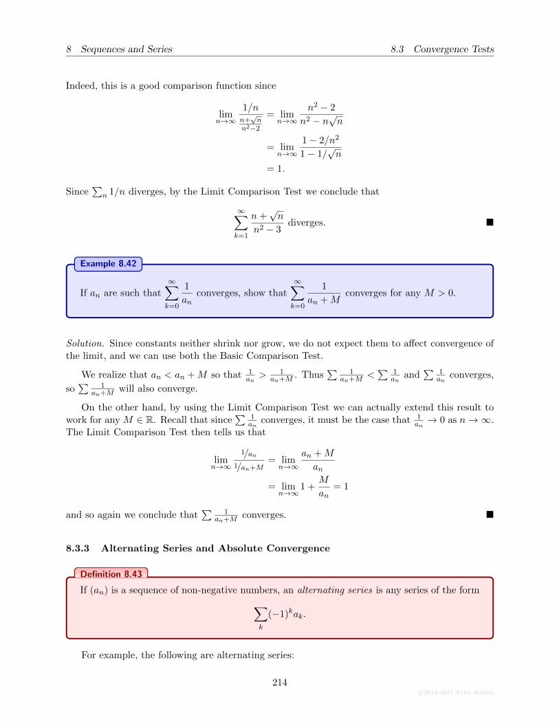
8 Sequences and Series 8.3 Convergence Tests
Indeed, this is a good comparison function since
limn→∞
1/nn+√n
n2−2
= limn→∞
n2 − 2
n2 − n√n
= limn→∞
1− 2/n2
1− 1/√n
= 1.
Since∑
n 1/n diverges, by the Limit Comparison Test we conclude that
∞∑
k=1
n+√n
n2 − 3diverges. �
Example 8.42
If an are such that∞∑
k=0
1
anconverges, show that
∞∑
k=0
1
an +Mconverges for any M > 0.
Solution. Since constants neither shrink nor grow, we do not expect them to affect convergence ofthe limit, and we can use both the Basic Comparison Test.
We realize that an < an +M so that 1an> 1
an+M . Thus∑ 1
an+M <∑ 1
anand
∑ 1an
converges,
so∑ 1
an+M will also converge.
On the other hand, by using the Limit Comparison Test we can actually extend this result towork for any M ∈ R. Recall that since
∑ 1an
converges, it must be the case that 1an→ 0 as n→∞.
The Limit Comparison Test then tells us that
limn→∞
1/an1/an+M
= limn→∞
an +M
an
= limn→∞
1 +M
an= 1
and so again we conclude that∑ 1
an+M converges. �
8.3.3 Alternating Series and Absolute Convergence
Definition 8.43
If (an) is a sequence of non-negative numbers, an alternating series is any series of the form
∑
k
(−1)kak.
For example, the following are alternating series:
214c©2013-2017 Tyler Holden
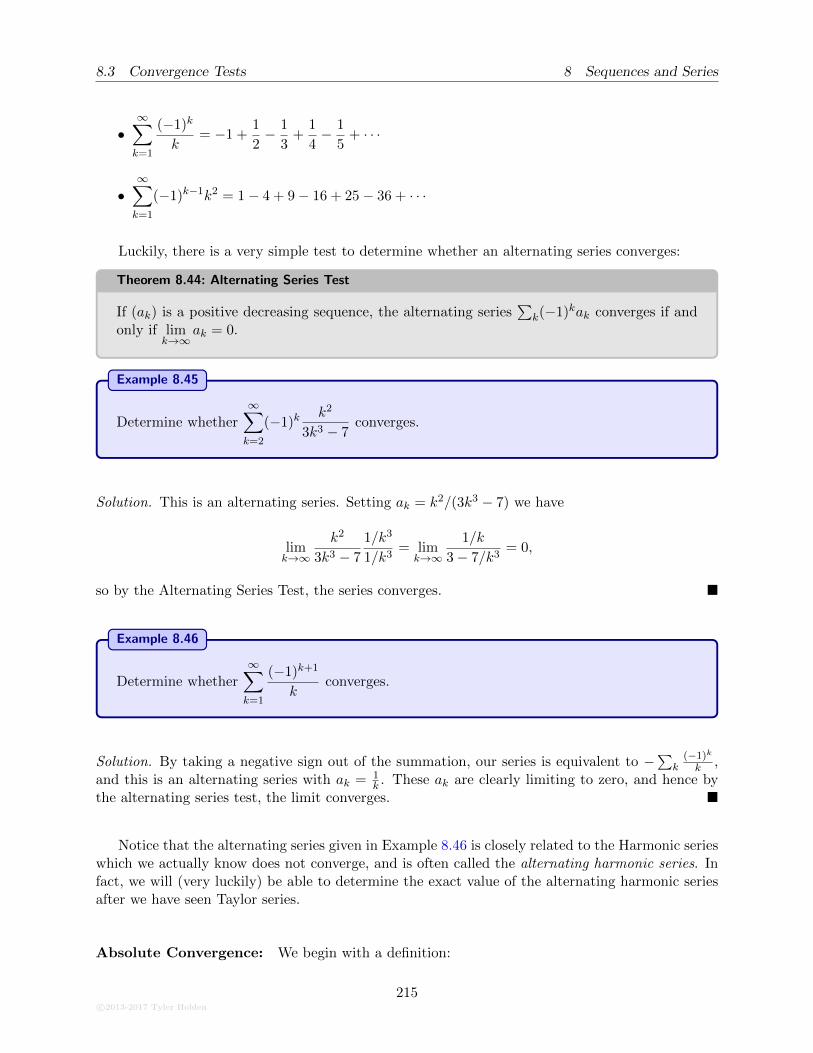
8.3 Convergence Tests 8 Sequences and Series
•∞∑
k=1
(−1)k
k= −1 +
1
2− 1
3+
1
4− 1
5+ · · ·
•∞∑
k=1
(−1)k−1k2 = 1− 4 + 9− 16 + 25− 36 + · · ·
Luckily, there is a very simple test to determine whether an alternating series converges:
Theorem 8.44: Alternating Series Test
If (ak) is a positive decreasing sequence, the alternating series∑
k(−1)kak converges if andonly if lim
k→∞ak = 0.
Example 8.45
Determine whether
∞∑
k=2
(−1)kk2
3k3 − 7converges.
Solution. This is an alternating series. Setting ak = k2/(3k3 − 7) we have
limk→∞
k2
3k3 − 7
1/k3
1/k3= lim
k→∞
1/k
3− 7/k3= 0,
so by the Alternating Series Test, the series converges. �
Example 8.46
Determine whether
∞∑
k=1
(−1)k+1
kconverges.
Solution. By taking a negative sign out of the summation, our series is equivalent to −∑k(−1)k
k ,and this is an alternating series with ak = 1
k . These ak are clearly limiting to zero, and hence bythe alternating series test, the limit converges. �
Notice that the alternating series given in Example 8.46 is closely related to the Harmonic serieswhich we actually know does not converge, and is often called the alternating harmonic series. Infact, we will (very luckily) be able to determine the exact value of the alternating harmonic seriesafter we have seen Taylor series.
Absolute Convergence: We begin with a definition:
c©2013-2017 Tyler Holden
215
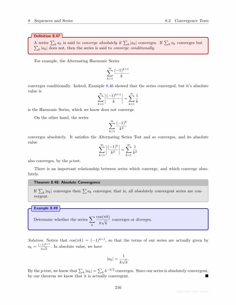
8 Sequences and Series 8.3 Convergence Tests
Definition 8.47
A series∑
k ak is said to converge absolutely if∑
k |ak| converges. If∑
k ak converges but∑k |ak| does not, then the series is said to converge conditionally.
For example, the Alternating Harmonic Series
∞∑
k=1
(−1)k+1
k
converges conditionally. Indeed, Example 8.46 showed that the series converged, but it’s absolutevalue is
∞∑
k=1
∣∣∣∣(−1)k+1
k
∣∣∣∣ =∞∑
k=1
1
k
is the Harmonic Series, which we know does not converge.
On the other hand, the series∞∑
k=1
(−1)k
k2
converges absolutely. It satisfies the Alternating Series Test and so converges, and its absolutevalue
∞∑
k=1
∣∣∣∣(−1)k
k2
∣∣∣∣ =
∞∑
k=1
1
k2
also converges, by the p-test.
There is an important relationship between series which converge, and which converge abso-lutely.
Theorem 8.48: Absolute Convergence
If∑
k |ak| converges then∑ak converges; that is, all absolutely convergent series are con-
vergent.
Example 8.49
Determine whether the series∑
k
cos(πk)
k√k
converges or diverges.
Solution. Notice that cos(πk) = (−1)k+1, so that the terms of our series are actually given by
ak = (−1)k+1
k√k
. In absolute value, we have
|ak| =1
k√k.
By the p-test, we know that∑
k |ak| =∑
k k−3/2 converges. Since our series is absolutely convergent,
by our theorem we know that it is actually convergent. �
216c©2013-2017 Tyler Holden
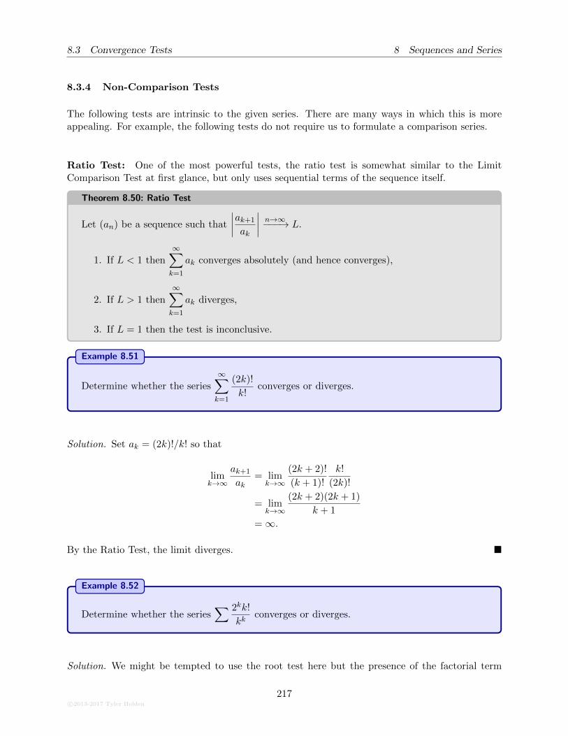
8.3 Convergence Tests 8 Sequences and Series
8.3.4 Non-Comparison Tests
The following tests are intrinsic to the given series. There are many ways in which this is moreappealing. For example, the following tests do not require us to formulate a comparison series.
Ratio Test: One of the most powerful tests, the ratio test is somewhat similar to the LimitComparison Test at first glance, but only uses sequential terms of the sequence itself.
Theorem 8.50: Ratio Test
Let (an) be a sequence such that
∣∣∣∣ak+1
ak
∣∣∣∣n→∞−−−→ L.
1. If L < 1 then∞∑
k=1
ak converges absolutely (and hence converges),
2. If L > 1 then
∞∑
k=1
ak diverges,
3. If L = 1 then the test is inconclusive.
Example 8.51
Determine whether the series
∞∑
k=1
(2k)!
k!converges or diverges.
Solution. Set ak = (2k)!/k! so that
limk→∞
ak+1
ak= lim
k→∞
(2k + 2)!
(k + 1)!
k!
(2k)!
= limk→∞
(2k + 2)(2k + 1)
k + 1
=∞.
By the Ratio Test, the limit diverges. �
Example 8.52
Determine whether the series∑ 2kk!
kkconverges or diverges.
Solution. We might be tempted to use the root test here but the presence of the factorial term
c©2013-2017 Tyler Holden
217
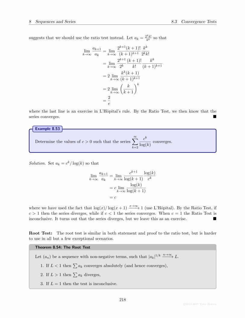
8 Sequences and Series 8.3 Convergence Tests
suggests that we should use the ratio test instead. Let ak = 2kk!kk
so that
limk→∞
ak+1
ak= lim
k→∞
2k+1(k + 1)!
(k + 1)k+1
kk
2kk!
= limk→∞
2k+1
2k(k + 1)!
k!
kk
(k + 1)k+1
= 2 limk→∞
kk(k + 1)
(k + 1)k+1
= 2 limk→∞
(k
k + 1
)k
=2
e
where the last line is an exercise in L’Hopital’s rule. By the Ratio Test, we then know that theseries converges. �
Example 8.53
Determine the values of c > 0 such that the series
∞∑
k=2
ck
log(k)converges.
Solution. Set ak = ck/ log(k) so that
limk→∞
ak+1
ak= lim
k→∞
ck+1
log(k + 1)
log(k)
ck
= c limk→∞
log(k)
log(k + 1)
= c
where we have used the fact that log(x)/ log(x+ 1)x→∞−−−→ 1 (use L’Hopital). By the Ratio Test, if
c > 1 then the series diverges, while if c < 1 the series converges. When c = 1 the Ratio Test isinconclusive. It turns out that the series diverges, but we leave this as an exercise. �
Root Test: The root test is similar in both statement and proof to the ratio test, but is harderto use in all but a few exceptional scenarios.
Theorem 8.54: The Root Test
Let (an) be a sequence with non-negative terms, such that |ak|1/k n→∞−−−→ L.
1. If L < 1 then∑ak converges absolutely (and hence converges),
2. If L > 1 then∑ak diverges,
3. If L = 1 then the test is inconclusive.
218c©2013-2017 Tyler Holden
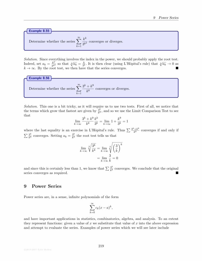
9 Power Series
Example 8.55
Determine whether the series∞∑
k=1
kk
3k2converges or diverges.
Solution. Since everything involves the index in the power, we should probably apply the root test.Indeed, set ak = kk
3k2so that k
√ak = k
3k. It is then clear (using L’Hopital’s rule) that k
√ak → 0 as
k →∞. By the root test, we then have that the series converges. �
Example 8.56
Determine whether the series
∞∑
k=1
3k + k9
kkconverges or diverges.
Solution. This one is a bit tricky, as it will require us to use two tests. First of all, we notice thatthe terms which grow that fastest are given by 3k
kk, and so we use the Limit Comparison Test to see
that
limk→∞
3k + k9
kkkk
3k= lim
k→∞1 +
k9
3k= 1
where the last equality is an exercise in L’Hopital’s rule. Thus∑ 3k+k9
kkconverges if and only if∑ 3k
kkconverges. Setting ak = 3k
kkthe root test tells us that
limk→∞
k
√3k
kk= lim
k→∞k
√(3
k
)k
= limk→∞
3
k= 0
and since this is certainly less than 1, we know that∑ 3k
kkconverges. We conclude that the original
series converges as required. �
9 Power Series
Power series are, in a sense, infinite polynomials of the form
∞∑
k=0
ck(x− a)k,
and have important applications in statistics, combinatorics, algebra, and analysis. To an extentthey represent functions: given a value of x we substitute that value of x into the above expressionand attempt to evaluate the series. Examples of power series which we will see later include
c©2013-2017 Tyler Holden
219
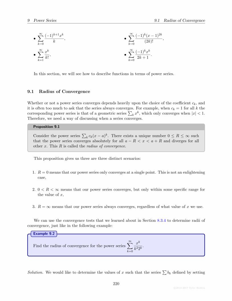
9 Power Series 9.1 Radius of Convergence
•∞∑
k=0
(−1)k+1xk
k,
•∞∑
k=1
xk
k!,
•∞∑
k=0
(−1)k(x− 1)2k
(2k)!,
•∞∑
k=0
(−1)kxk
2k + 1.
In this section, we will see how to describe functions in terms of power series.
9.1 Radius of Convergence
Whether or not a power series converges depends heavily upon the choice of the coefficient ck, andit is often too much to ask that the series always converges. For example, when ck = 1 for all k thecorresponding power series is that of a geometric series
∑k x
k, which only converges when |x| < 1.Therefore, we need a way of discussing when a series converges.
Proposition 9.1
Consider the power series∑
k ck(x − a)k. There exists a unique number 0 ≤ R ≤ ∞ suchthat the power series converges absolutely for all a − R < x < a + R and diverges for allother x. This R is called the radius of convergence.
This proposition gives us three are three distinct scenarios:
1. R = 0 means that our power series only converges at a single point. This is not an enlighteningcase,
2. 0 < R < ∞ means that our power series converges, but only within some specific range forthe value of x,
3. R =∞ means that our power series always converges, regardless of what value of x we use.
We can use the convergence tests that we learned about in Section 8.3.4 to determine radii ofconvergence, just like in the following example:
Example 9.2
Find the radius of convergence for the power series
∞∑
k=0
xk
k22k.
Solution. We would like to determine the values of x such that the series∑bk defined by setting
220c©2013-2017 Tyler Holden
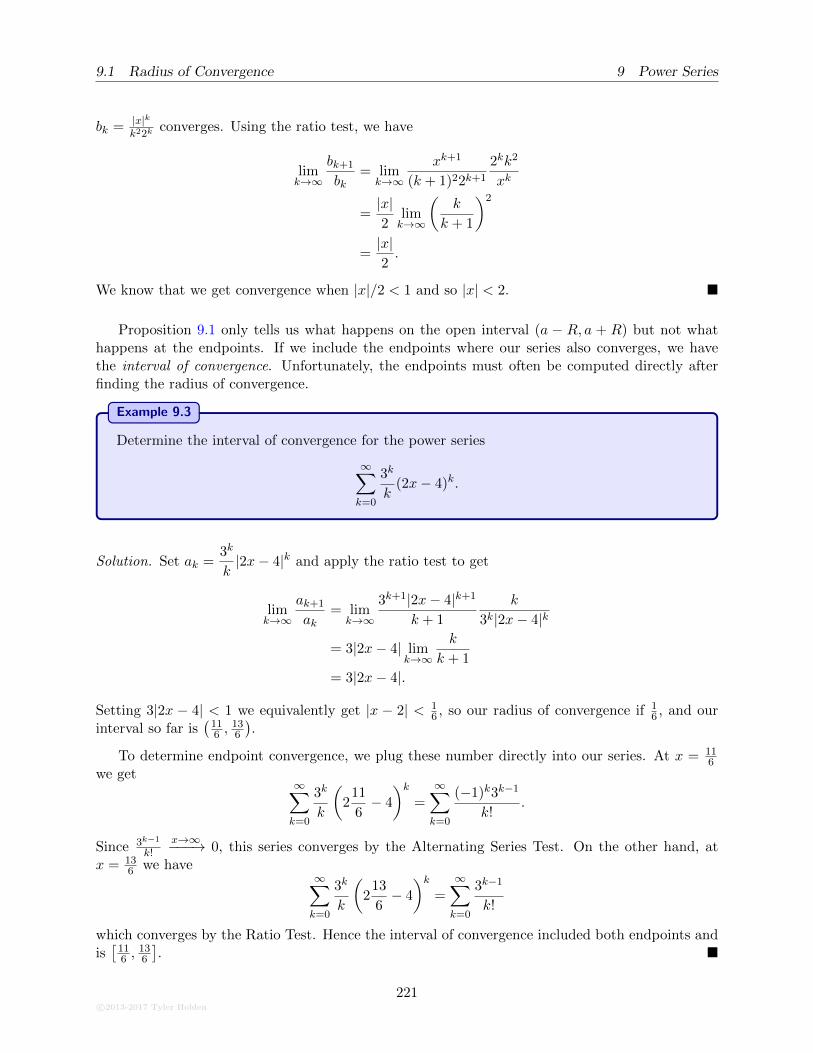
9.1 Radius of Convergence 9 Power Series
bk = |x|kk22k
converges. Using the ratio test, we have
limk→∞
bk+1
bk= lim
k→∞
xk+1
(k + 1)22k+1
2kk2
xk
=|x|2
limk→∞
(k
k + 1
)2
=|x|2.
We know that we get convergence when |x|/2 < 1 and so |x| < 2. �
Proposition 9.1 only tells us what happens on the open interval (a − R, a + R) but not whathappens at the endpoints. If we include the endpoints where our series also converges, we havethe interval of convergence. Unfortunately, the endpoints must often be computed directly afterfinding the radius of convergence.
Example 9.3
Determine the interval of convergence for the power series
∞∑
k=0
3k
k(2x− 4)k.
Solution. Set ak =3k
k|2x− 4|k and apply the ratio test to get
limk→∞
ak+1
ak= lim
k→∞
3k+1|2x− 4|k+1
k + 1
k
3k|2x− 4|k
= 3|2x− 4| limk→∞
k
k + 1
= 3|2x− 4|.
Setting 3|2x − 4| < 1 we equivalently get |x − 2| < 16 , so our radius of convergence if 1
6 , and ourinterval so far is
(116 ,
136
).
To determine endpoint convergence, we plug these number directly into our series. At x = 116
we get∞∑
k=0
3k
k
(2
11
6− 4
)k=
∞∑
k=0
(−1)k3k−1
k!.
Since 3k−1
k!x→∞−−−→ 0, this series converges by the Alternating Series Test. On the other hand, at
x = 136 we have
∞∑
k=0
3k
k
(2
13
6− 4
)k=∞∑
k=0
3k−1
k!
which converges by the Ratio Test. Hence the interval of convergence included both endpoints andis[
116 ,
136
]. �
c©2013-2017 Tyler Holden
221
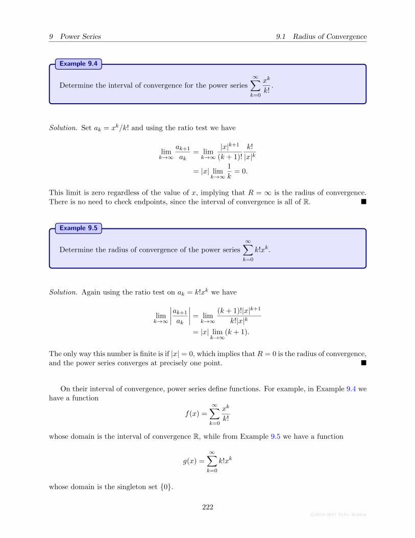
9 Power Series 9.1 Radius of Convergence
Example 9.4
Determine the interval of convergence for the power series∞∑
k=0
xk
k!.
Solution. Set ak = xk/k! and using the ratio test we have
limk→∞
ak+1
ak= lim
k→∞
|x|k+1
(k + 1)!
k!
|x|k
= |x| limk→∞
1
k= 0.
This limit is zero regardless of the value of x, implying that R = ∞ is the radius of convergence.There is no need to check endpoints, since the interval of convergence is all of R. �
Example 9.5
Determine the radius of convergence of the power series
∞∑
k=0
k!xk.
Solution. Again using the ratio test on ak = k!xk we have
limk→∞
∣∣∣∣ak+1
ak
∣∣∣∣ = limk→∞
(k + 1)!|x|k+1
k!|x|k= |x| lim
k→∞(k + 1).
The only way this number is finite is if |x| = 0, which implies that R = 0 is the radius of convergence,and the power series converges at precisely one point. �
On their interval of convergence, power series define functions. For example, in Example 9.4 wehave a function
f(x) =∞∑
k=0
xk
k!
whose domain is the interval of convergence R, while from Example 9.5 we have a function
g(x) =∞∑
k=0
k!xk
whose domain is the singleton set {0}.
222c©2013-2017 Tyler Holden
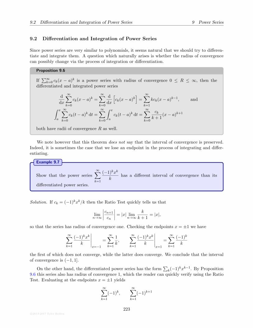
9.2 Differentiation and Integration of Power Series 9 Power Series
9.2 Differentiation and Integration of Power Series
Since power series are very similar to polynomials, it seems natural that we should try to differen-tiate and integrate them. A question which naturally arises is whether the radius of convergencecan possibly change via the process of integration or differentiation.
Proposition 9.6
If∑∞
k=0 ck(x − a)k is a power series with radius of convergence 0 ≤ R ≤ ∞, then thedifferentiated and integrated power series
d
dx
∞∑
k=0
ck(x− a)k =
∞∑
k=0
d
dx
[ck(x− a)k
]=∞∑
k=1
kck(x− a)k−1, and
∫ x
a
∞∑
k=0
ck(t− a)k dt =
∞∑
k=0
∫ x
ack(t− a)k dt =
∞∑
k=0
ckk + 1
(x− a)k+1
both have radii of convergence R as well.
We note however that this theorem does not say that the interval of convergence is preserved.Indeed, it is sometimes the case that we lose an endpoint in the process of integrating and differ-entiating.
Example 9.7
Show that the power series
∞∑
k=1
(−1)kxk
khas a different interval of convergence than its
differentiated power series.
Solution. If ck = (−1)kxk/k then the Ratio Test quickly tells us that
limn→∞
∣∣∣∣cn+1
cn
∣∣∣∣ = |x| limn→∞
k
k + 1= |x|,
so that the series has radius of convergence one. Checking the endpoints x = ±1 we have
∞∑
k=1
(−1)kxk
k
∣∣∣∣∣x=−1
=
∞∑
k=1
1
k,
∞∑
k=1
(−1)kxk
k
∣∣∣∣∣x=1
=
∞∑
k=1
(−1)k
k
the first of which does not converge, while the latter does converge. We conclude that the intervalof convergence is (−1, 1].
On the other hand, the differentiated power series has the form∑
k(−1)kxk−1. By Proposition9.6 this series also has radius of convergence 1, which the reader can quickly verify using the RatioTest. Evaluating at the endpoints x = ±1 yields
∞∑
k=1
(−1)k,∞∑
k=1
(−1)k+1
c©2013-2017 Tyler Holden
223
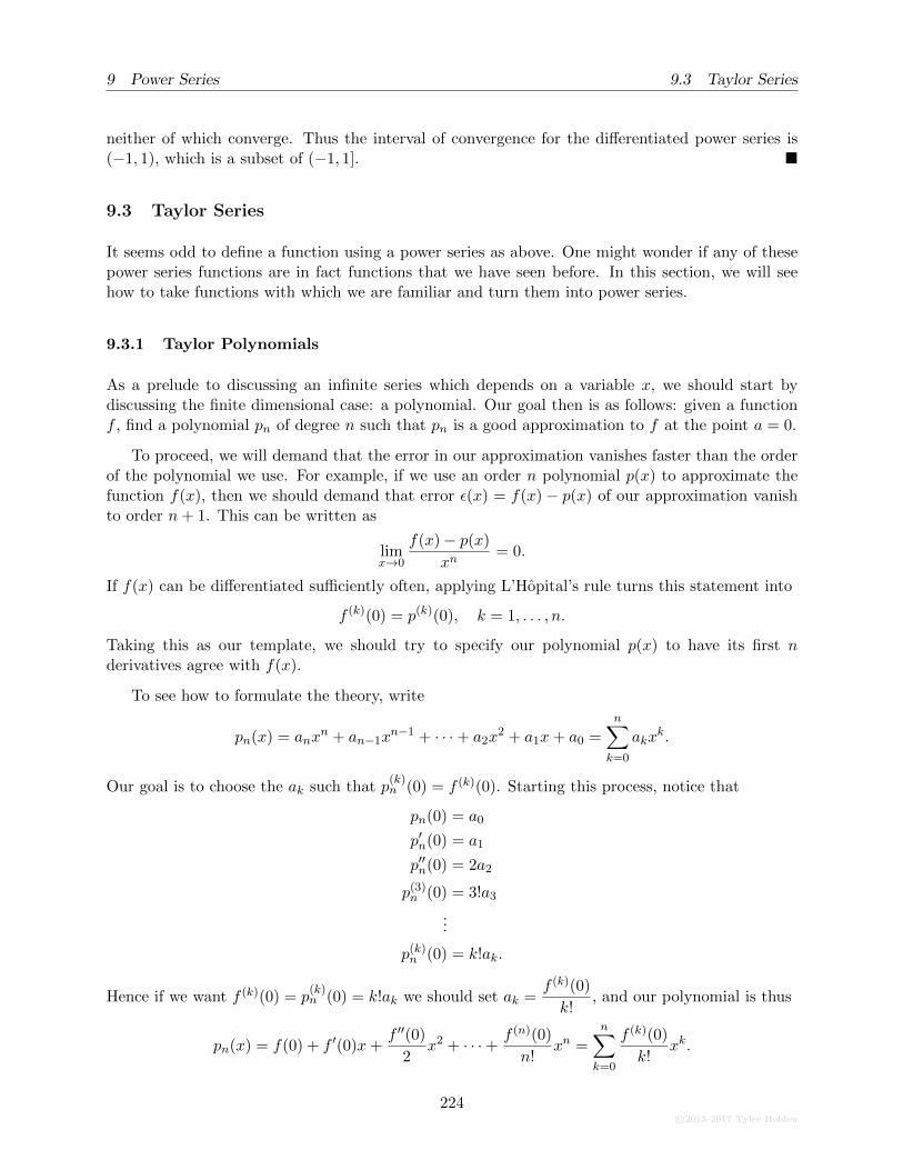
9 Power Series 9.3 Taylor Series
neither of which converge. Thus the interval of convergence for the differentiated power series is(−1, 1), which is a subset of (−1, 1]. �
9.3 Taylor Series
It seems odd to define a function using a power series as above. One might wonder if any of thesepower series functions are in fact functions that we have seen before. In this section, we will seehow to take functions with which we are familiar and turn them into power series.
9.3.1 Taylor Polynomials
As a prelude to discussing an infinite series which depends on a variable x, we should start bydiscussing the finite dimensional case: a polynomial. Our goal then is as follows: given a functionf , find a polynomial pn of degree n such that pn is a good approximation to f at the point a = 0.
To proceed, we will demand that the error in our approximation vanishes faster than the orderof the polynomial we use. For example, if we use an order n polynomial p(x) to approximate thefunction f(x), then we should demand that error ε(x) = f(x) − p(x) of our approximation vanishto order n+ 1. This can be written as
limx→0
f(x)− p(x)
xn= 0.
If f(x) can be differentiated sufficiently often, applying L’Hopital’s rule turns this statement into
f (k)(0) = p(k)(0), k = 1, . . . , n.
Taking this as our template, we should try to specify our polynomial p(x) to have its first nderivatives agree with f(x).
To see how to formulate the theory, write
pn(x) = anxn + an−1x
n−1 + · · ·+ a2x2 + a1x+ a0 =
n∑
k=0
akxk.
Our goal is to choose the ak such that p(k)n (0) = f (k)(0). Starting this process, notice that
pn(0) = a0
p′n(0) = a1
p′′n(0) = 2a2
p(3)n (0) = 3!a3
...
p(k)n (0) = k!ak.
Hence if we want f (k)(0) = p(k)n (0) = k!ak we should set ak =
f (k)(0)
k!, and our polynomial is thus
pn(x) = f(0) + f ′(0)x+f ′′(0)
2x2 + · · ·+ f (n)(0)
n!xn =
n∑
k=0
f (k)(0)
k!xk.
224c©2013-2017 Tyler Holden
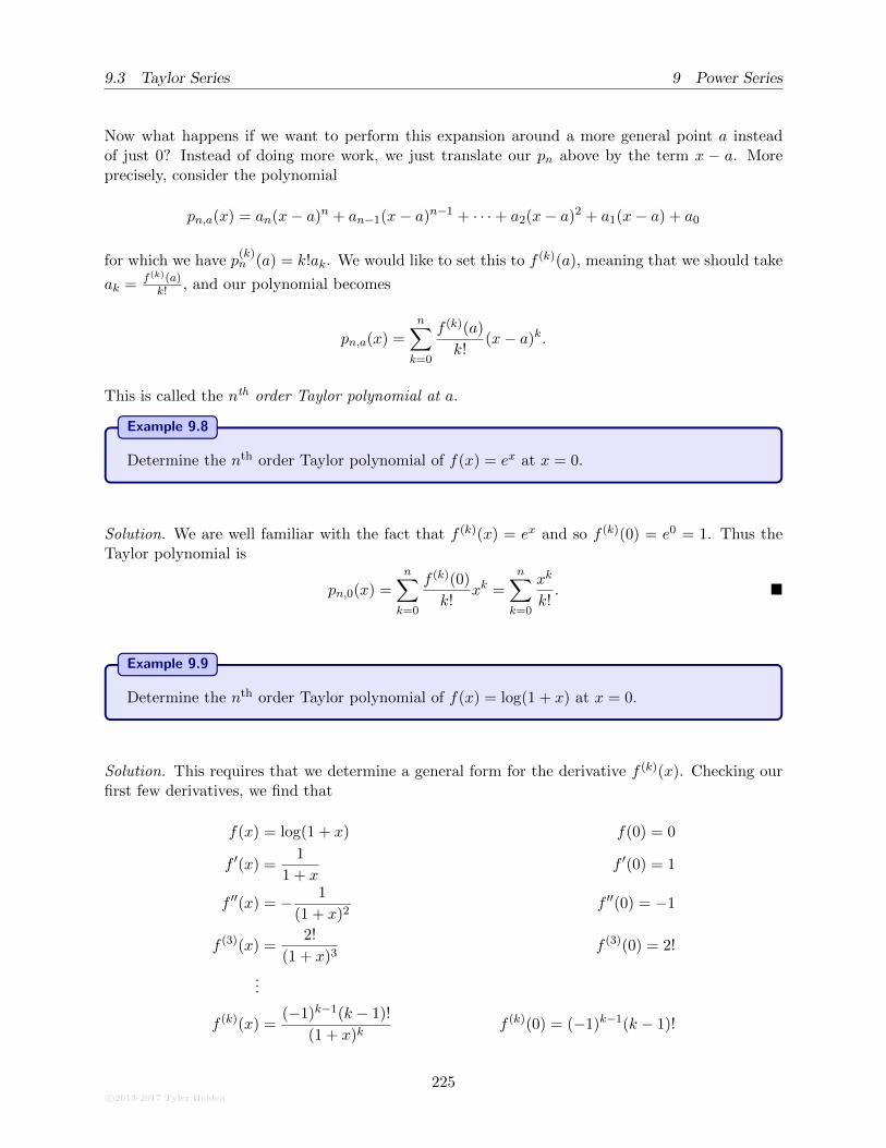
9.3 Taylor Series 9 Power Series
Now what happens if we want to perform this expansion around a more general point a insteadof just 0? Instead of doing more work, we just translate our pn above by the term x − a. Moreprecisely, consider the polynomial
pn,a(x) = an(x− a)n + an−1(x− a)n−1 + · · ·+ a2(x− a)2 + a1(x− a) + a0
for which we have p(k)n (a) = k!ak. We would like to set this to f (k)(a), meaning that we should take
ak = f (k)(a)k! , and our polynomial becomes
pn,a(x) =
n∑
k=0
f (k)(a)
k!(x− a)k.
This is called the nth order Taylor polynomial at a.
Example 9.8
Determine the nth order Taylor polynomial of f(x) = ex at x = 0.
Solution. We are well familiar with the fact that f (k)(x) = ex and so f (k)(0) = e0 = 1. Thus theTaylor polynomial is
pn,0(x) =
n∑
k=0
f (k)(0)
k!xk =
n∑
k=0
xk
k!. �
Example 9.9
Determine the nth order Taylor polynomial of f(x) = log(1 + x) at x = 0.
Solution. This requires that we determine a general form for the derivative f (k)(x). Checking ourfirst few derivatives, we find that
f(x) = log(1 + x) f(0) = 0
f ′(x) =1
1 + xf ′(0) = 1
f ′′(x) = − 1
(1 + x)2f ′′(0) = −1
f (3)(x) =2!
(1 + x)3f (3)(0) = 2!
...
f (k)(x) =(−1)k−1(k − 1)!
(1 + x)kf (k)(0) = (−1)k−1(k − 1)!
c©2013-2017 Tyler Holden
225

9 Power Series 9.3 Taylor Series
The veracity of this most general form can be checked by induction, and is left as an exercise forthe student. Hence the nth-order Taylor polynomial is
pn,0(x) =
n∑
k=0
f (k)(0)
k!xk =
n∑
k=0
(−1)k−1(k − 1)!
k!xk
=
n∑
k=0
(−1)k−1
kxk. �
Example 9.10
Compute the Taylor polynomial of x sin(x) about 0.
Solution. It will quickly become laborious for us to differentiate the function f(x) = x sin(x), and infact it will be effectively impossible to derive a closed form expression for a generic n-th derivative.Instead, the Taylor polynomial of x is just x itself, so we need only compute the Taylor polynomialof sin(x).
We know that
sin(0) = 0 d2
dx2
∣∣∣x=0
sin(x) = − sin(x)|x=0 = 0
ddx sin(x)
∣∣x=0
= cos(x)|x=0 = 1 d3
dx3
∣∣∣x=0
= − cos(x)|x=0 = −1.
Since the derivatives of sine repeat with periodicity 4, this is all we need to compute. In particularthough, we notice that only the odd terms will survive, and they will switch sign. By writingour odd numbers as 2n + 1, the sign of the 2n + 1-st derivative is (−1)n and we get the Taylorpolynomial (or order 2n+ 1)
sin(x) =n∑
k=0
(−1)n
(2n+ 1)!x2n+1.
The Taylor polynomial of x sin(x) is thus
x sin(x) = x
n∑
k=0
(−1)n
(2n+ 1)!x2n+1 =
n∑
k=0
(−1)n
(2n+ 1)!x2n+2. �
9.3.2 Taylor Series
By extending the idea of Taylor polynomials to power series, we get the definition of the Taylorseries of the function f about the point x = a. In particular, consider the following result:
226c©2013-2017 Tyler Holden
9.3 Taylor Series 9 Power Series
Theorem 9.11
Let f(x) be an infinitely differentiable function and consider the power series defined by
∞∑
k=0
f (k)(a)
k!(x− a)k.
If I is the interval of convergence of this power series, then for every x ∈ I we have
f(x) =∞∑
k=0
f (k)(a)
k!(x− a)k.
That is, on its interval of convergence, a function is equal to the value of its Taylor series.
We say that the function f is analytic at the point c if the Taylor series at f has a non-zeroradius of convergence at c. If f is analytic at every c ∈ R, we just say that f is analytic.
One must be careful to realize that infinitely differentiable is not the same thing as analytic.Define the function
f(x) =
{e−
1x x > 0
0 x ≤ 0.
This function is infinitely differentiable. However, it is not analytic at x = 0. With a bit of work,one can show that the Taylor series of f(x) at 0 has radius of convergence 0.
1. ex =∞∑
k=0
xk
k!, interval of convergence R.
2. sin(x) =∞∑
k=0
(−1)kx2k+1
(2k + 1)!, cos(x) =
∞∑
k=0
(−1)kx2k
(2k)!, interval of convergence R.
3.1
1− x =
∞∑
k=0
xk, interval of convergence (−1, 1).
4. log(1 + x) =∞∑
k=1
(−1)k+1xk
k, interval of convergence (−1, 1].
5. arctan(x) =∞∑
k=0
(−1)kx2k+1
2k + 1, interval of convergence (−1, 1].
An easy way to remember property (2): we know sin(x) is odd as a function, and indeed itsTaylor series only has powers in odd order. Similarly, cos(x) is even as a function and its Taylorseries only has powers of even order. We are not yet in a position to compute (5), but we provideit here as an interesting and motivating example which we will use (and prove) later.
It is worth noting that I am cheating here. Theorem 9.11 only tells us that the function isequal to its Taylor series on the interior of the interval of convergence and not at the endpoints.
c©2013-2017 Tyler Holden
227
9 Power Series 9.4 Differentiation and Integration of Taylor Series
It is another theorem to show that if convergence holds at the endpoints then the function stillconverges there, but let’s sweep that under the rug for now.
Exercise: Notice how the Taylor series for ex looks very similar to the Taylor series for sin(x)and cos(x). Indeed, if we ignore the (−1)k terms we see that sin(x) contains the odd terms ofex while cos(x) contains the even terms. If we can account for these minus signs, maybe wecan get a relationship between a priori unrelated exponential function and the trigonometricfunctions.
1. Recall that in the complex numbers, we can define a number i such that i2 = −1.Using their Taylor series expansions, show that eix = cos(x) + i sin(x).
2. We know that every point on the unit circle can be written as (cos(θ), sin(θ)) where θ isthe angle between the point and the positive x-axis. If we think about cos(x) + i sin(x)as (cos(x), sin(x)) convince yourself that eix sweeps out the unit circle as x traversesthrough [0, 2π).
9.4 Differentiation and Integration of Taylor Series
So far we have seen that functions have power series representations on their radius of convergence.Moreover, Theorem 9.6 told us that we could integrate and differentiate power series while preservertheir radius of convergence.
Combining these two results means that we we can interchange the summation sign with thederivative/integral. Indeed,
f ′(x) =d
dxf(x) =
d
dx
∞∑
k=0
akxk =
∞∑
k=0
ak
[d
dxxk]
=∞∑
k=1
kakxk−1,
and similarly for integration. This is not the same thing as linearity, and we should not assumethat this result follows immediately. We encourage the student to accept the theorem as stated,but not to underestimate the subtlety of the situation.
Example 9.12
Using the fact that1
1− x =
∞∑
k=0
xk on (−1, 1), show that log(1 + x) =
∞∑
k=1
(−1)k−1xk
kon
(−1, 1).
Solution. Note that the Taylor series for 1/(1 + x) can be derived from 1/(1 − x) by substituting−x into the Taylor series:
1
1 + x=
1
1− (−x)=
∞∑
k=0
(−x)k =
∞∑
k=0
(−1)kxk.
Now we know that ∫ x
0
1
1 + tdt = log(1 + x)
228c©2013-2017 Tyler Holden
9.5 Applications of Taylor Series 9 Power Series
so applying a term-by-term integration, we get
log(1 + x) =
∫ x
0
1
1 + tdt =
∫ x
0
∞∑
k=0
(−1)ktk dt
=
∞∑
k=0
(−1)k∫ x
0tk dt =
∞∑
k=0
(−1)ktk+1
k + 1
∣∣∣∣∣
t=x
t=0
=
∞∑
k=1
(−1)k−1xk
k
where in the last line we have re-indexed the sum. �
Example 9.13
Confirm that the Taylor series of arctan(x) is given by∞∑
k=0
(−1)kx2k+1
2k + 1.
Solution. We know that arctan(x) =
∫ x
0
1
1 + t2dx, and we know the Taylor series for 1
1+t2since it
is given by
1
1 + t2=
1
1− (−t2)=∞∑
k=0
(−t2)k =∞∑
k=0
(−1)kt2k.
Integrating term by term, we get
arctan(x) =∞∑
k=0
∫ x
0(−1)kt2kdt =
∞∑
k=0
(−1)kx2k+1
2k + 1
as required. �
9.5 Applications of Taylor Series
Calculators and calculating: One of the historic applications of power series is the ability tocompute the value of a function to arbitrary precision in terms of polynomials. In the case oftranscendental functions especially (such as log, sin, cos, exp), this is how modern day computersand calculators often compute values.
Computing Limits and Asymptotics: Mathematicians often cheat when looking at limits, inthe sense that we can often guess that value of the limit if we know a little something about theTaylor series of the terms involved.
Before proceeding, let us introduce a little notation. If f(x) and g(x) are functions, we say thatthat f(x) = o(g(x)) if f(x) and g(x) grow at the same rate; that is, f(x) and g(x) shared the sameasymptotics in the limit as f(x) and g(x) go to infinity. In a similar vein, we may define ‘big-O’
c©2013-2017 Tyler Holden
229
9 Power Series 9.5 Applications of Taylor Series
notation as describing the asymptotics of f(x) and g(x) when they go to zero 14. In effect, we willwrite f(x) = O(g(x)) if f(x) is at worst g(x) in the limit as x→ 0. For example, the Taylor seriesof ex is
ex =∞∑
k=0
xk
k!.
If we are playing with numbers very near zero, and are only interested in what is happening up tothe quadratic term, we might write this as
ex = 1 + x+x2
2+O(x3)
where here O(x3) indicates that the dominant factor in the error is of order x3 (for x near 0, theterm x4 will be much smaller than x3, and so on). When taking limits as x → 0, anything withO(xk) k ≥ 1 will vanish, meaning that we are only interested in the constant terms.
Now we often used Taylor series to create L’Hopital problems, such as the following:
Example 9.14
Consider the limit limx→0
ex − 1− xx2
.
Solution. When we made this example, we used the fact that we knew what the Taylor series forex. Indeed, the numerator becomes
ex − 1− x =
(1 + x+
x2
2+O(x3)
)− 1− x =
x2
2!+O(x3).
Hence applying this to the limit, we have
limx→0
ex − 1− xx2
= limx→0
x2
2! +O(x3)
x2
= limx→0
[1
2!+O(x)
]
=1
2.
One can check this is the same answer we get by applying L’Hopital. �
Example 9.15
(Example 4.24) Determine the limit limx→0
xenx − x1− cos(nx)
for n 6= 0.
14There is also a version of big-O for infinite asymptotics.
230c©2013-2017 Tyler Holden
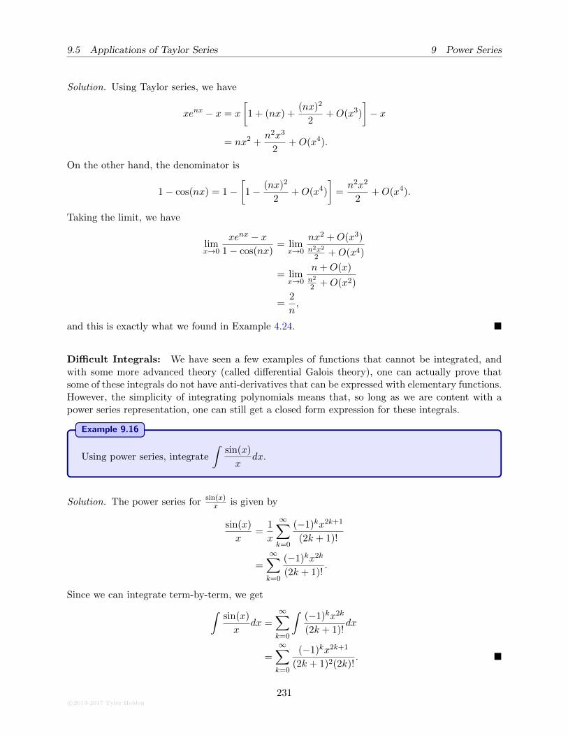
9.5 Applications of Taylor Series 9 Power Series
Solution. Using Taylor series, we have
xenx − x = x
[1 + (nx) +
(nx)2
2+O(x3)
]− x
= nx2 +n2x3
2+O(x4).
On the other hand, the denominator is
1− cos(nx) = 1−[1− (nx)2
2+O(x4)
]=n2x2
2+O(x4).
Taking the limit, we have
limx→0
xenx − x1− cos(nx)
= limx→0
nx2 +O(x3)n2x2
2 +O(x4)
= limx→0
n+O(x)n2
2 +O(x2)
=2
n,
and this is exactly what we found in Example 4.24. �
Difficult Integrals: We have seen a few examples of functions that cannot be integrated, andwith some more advanced theory (called differential Galois theory), one can actually prove thatsome of these integrals do not have anti-derivatives that can be expressed with elementary functions.However, the simplicity of integrating polynomials means that, so long as we are content with apower series representation, one can still get a closed form expression for these integrals.
Example 9.16
Using power series, integrate
∫sin(x)
xdx.
Solution. The power series for sin(x)x is given by
sin(x)
x=
1
x
∞∑
k=0
(−1)kx2k+1
(2k + 1)!
=
∞∑
k=0
(−1)kx2k
(2k + 1)!.
Since we can integrate term-by-term, we get
∫sin(x)
xdx =
∞∑
k=0
∫(−1)kx2k
(2k + 1)!dx
=
∞∑
k=0
(−1)kx2k+1
(2k + 1)2(2k)!. �
c©2013-2017 Tyler Holden
231
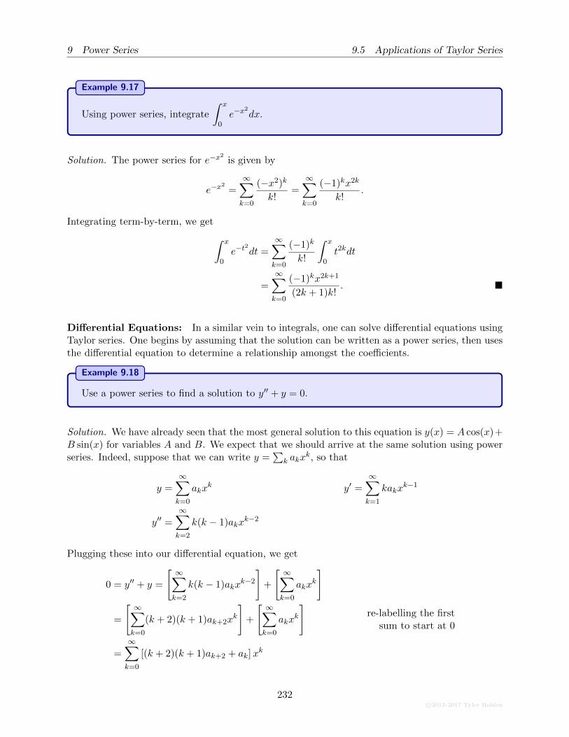
9 Power Series 9.5 Applications of Taylor Series
Example 9.17
Using power series, integrate
∫ x
0e−x
2dx.
Solution. The power series for e−x2
is given by
e−x2
=∞∑
k=0
(−x2)k
k!=∞∑
k=0
(−1)kx2k
k!.
Integrating term-by-term, we get
∫ x
0e−t
2dt =
∞∑
k=0
(−1)k
k!
∫ x
0t2kdt
=
∞∑
k=0
(−1)kx2k+1
(2k + 1)k!. �
Differential Equations: In a similar vein to integrals, one can solve differential equations usingTaylor series. One begins by assuming that the solution can be written as a power series, then usesthe differential equation to determine a relationship amongst the coefficients.
Example 9.18
Use a power series to find a solution to y′′ + y = 0.
Solution. We have already seen that the most general solution to this equation is y(x) = A cos(x)+B sin(x) for variables A and B. We expect that we should arrive at the same solution using powerseries. Indeed, suppose that we can write y =
∑k akx
k, so that
y =∞∑
k=0
akxk y′ =
∞∑
k=1
kakxk−1
y′′ =∞∑
k=2
k(k − 1)akxk−2
Plugging these into our differential equation, we get
0 = y′′ + y =
[ ∞∑
k=2
k(k − 1)akxk−2
]+
[ ∞∑
k=0
akxk
]
=
[ ∞∑
k=0
(k + 2)(k + 1)ak+2xk
]+
[ ∞∑
k=0
akxk
]re-labelling the first
sum to start at 0
=∞∑
k=0
[(k + 2)(k + 1)ak+2 + ak]xk
232c©2013-2017 Tyler Holden
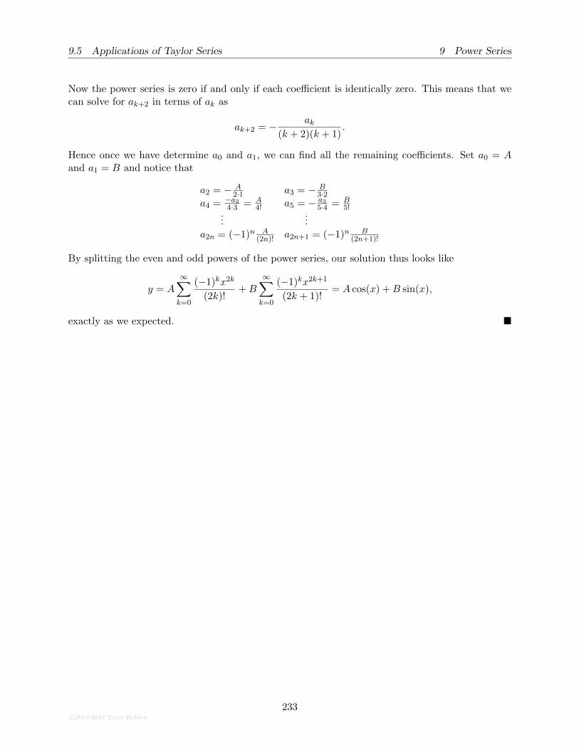
9.5 Applications of Taylor Series 9 Power Series
Now the power series is zero if and only if each coefficient is identically zero. This means that wecan solve for ak+2 in terms of ak as
ak+2 = − ak(k + 2)(k + 1)
.
Hence once we have determine a0 and a1, we can find all the remaining coefficients. Set a0 = Aand a1 = B and notice that
a2 = − A2·1 a3 = − B
3·2a4 = −a2
4·3 = A4! a5 = − a3
5·4 = B5!
......
a2n = (−1)n A(2n)! a2n+1 = (−1)n B
(2n+1)!
By splitting the even and odd powers of the power series, our solution thus looks like
y = A∞∑
k=0
(−1)kx2k
(2k)!+B
∞∑
k=0
(−1)kx2k+1
(2k + 1)!= A cos(x) +B sin(x),
exactly as we expected. �
c©2013-2017 Tyler Holden
233


![Discrete calculus, introduction · Discrete calculus, introduction Tristan Roussillon 09/09/2013 [GP2010] Leo J. Grady and Jonathan R. Polimeni. Discrete calculus. Applied analysis](https://img.pdfslide.net/doc/110x75/5f0f8efe7e708231d444c25d/discrete-calculus-introduction-discrete-calculus-introduction-tristan-roussillon.jpg)