Match Graph Construction for Large Image Databases

Match Graph Construction for Large Image Databases

Kwang In Kim1, James Tompkin1,2,3,Martin Theobald1, Jan Kautz2, and Christian Theobalt1

1Max-Planck-Institut fur Informatik, Campus E1 4, 66123 Saarbrucken, Germany2University College London, Malet Place, WC1E 6BT London, UK

3Intel Visual Computing Institute, Campus E2 1, 66123 Saarbrucken, Germany

Abstract. How best to efficiently establish correspondence among a large set ofimages or video frames is an interesting unanswered question. For large databases,the high computational cost of performing pair-wise image matching is a ma-jor problem. However, for many applications, images are inherently sparselyconnected, and so current techniques try to correctly estimate small potentiallymatching subsets of databases upon which to perform expensive pair-wise match-ing. Our contribution is to pose the identification of potential matches as a linkprediction problem in an image correspondence graph, and to propose an effec-tive algorithm to solve this problem. Our algorithm facilitates incremental imagematching: initially, the match graph is very sparse, but it becomes dense as we al-ternate between link prediction and verification. We demonstrate the effectivenessof our algorithm by comparing it with several existing alternatives on large-scaledatabases. Our resulting match graph is useful for many different applications.As an example, we show the benefits of our graph construction method to a labelpropagation application which propagates user-provided sparse object labels toother instances of that object in large image collections.

Keywords: Image matching, graph construction, link prediction

1 Introduction

The widespread use of digital still and video cameras and the success of social Webservices such as Facebook, Flickr, and YouTube has resulted in an enormous amountof publicly available image and video data. Organizing and browsing such large-scalevisual data (100,000+ images) is more than ever a pertinent problem in computer visionand data mining research. While there have been remarkable developments in the lastten years [1–6], structuring large-scale visual data is still an active research area andany improvements would have wide applicability.

The first step required to organize, annotate, and retrieve from large image and videocollections is to establish correspondences among individual images and video frames.This is not only an interesting problem by itself [3], but is also a key component to manypotential applications including 3D reconstruction [1, 7, 8], graphical navigation [3, 2],and content-based retrieval [9]. Establishing image correspondence in unconstraineddatabases is very challenging because of significant variations in the appearances ofobjects. We focus on the specific case where images are connected by static objectsappearing therein, e.g., landmarks and buildings, and this is assumed in most previous

2 Kim, K. I., Tompkin, J., Theobald, M., Kautz, J., and Theobalt, C.

work [1, 7, 3, 2]. This allows us to exploit well-established 3D geometry-based imagematching techniques [10]. However, our graph construction technique is general anddoes not depend on any particular matching technique or data content.

A significant problem with 3D geometry-based matching techniques (as well asother accurate image matching techniques) is that they are computationally expensiveand cannot feasibly be applied brute force to large-scale data. Fortunately, for the ap-plications we foresee, our data are inherently sparsely connected. Typically, an imagematches only a small subset of the entire database as, for example, photos of city land-marks are naturally geographically separated. We take advantage of this sparsity toquickly estimate a small subset of potential matches and then only verify these withan expensive matching procedure. This saves a significant amount of time versus per-forming an exhaustive pair-wise matching for a large-scale graph. Further, for manyapplications, it is useful that our iterative approach produces intermediate results (i.e.,only a subset of the entire set of potential matches are identified), allowing services tobe provided before computation is complete. Our algorithm is especially useful in thiscase since it maximizes the number of verified matches given a limited amount of timeand computational resources.

Our main contribution is an algorithm which predicts the existence of links amonga large set of potential matching candidates. We regard the process of matching asa graph construction where an edge between two nodes (a pair of images) indicatesa successful image match. Our system incrementally constructs a graph by iteratingbetween the estimation of potential links and their verification. In our experiments,we demonstrate that our algorithm well-predicts the existence of links and so enablesvery efficient use of computational resources in the matching stage. This avoids thetremendous task of matching all pairs of images a priori. We also demonstrate that ourapproach outperforms existing methods on two real-world databases.

Finally, we show how our graph construction can benefit an example application.Here, we choose label propagation: The labels (or annotations) are provided by usersfor some objects in some images. These labels are typically extremely sparse: as ex-tensive object labeling across an image or video collection is often infeasible, a usermay label an object (e.g., ‘London Eye’) in only a few keyframes in one video. Ouralgorithm automatically propagates sparse user-provided label data to large unstruc-tured image and video collections. The resulting algorithm enables users to easily sharelabels between visual data, i.e., to automatically assign labels to as many objects oc-currences as possible. Our label propagation framework also includes (semi-automatic)error correction, active label acquisition, and image-based query processing.

2 Related work

Our proposed graph construction algorithm is influenced by many techniques from dif-ferent disciplines. As such, in the first part of this section we focus only on reviewingwork related to organizing images, and we leave a review of data mining research forSec. 3.2. The second part of this section focuses on reviewing related label propagationalgorithms, as we use this application as an example of where our graph constructioncan benefit.

Match Graph Construction for Large Image Databases 3

Graph construction for images Many aspects of image and video organization arebased on a graph structure which encodes the match relations among a given set ofimages [3, 2, 7, 11]. While there are various choices of algorithm for matching pairsof images, 3D geometry-based matching is particularly relevant when a high level ofaccuracy is required. To deal with the high computational complexity of 3D geometry-based matching techniques, existing works typically adopt a pre-processing stage toquickly identify a small set of candidates which are later refined with geometry-basedmatching [3, 11, 7]. For large-scale image collections depicting heterogeneous regions,this approach by itself may not be sufficient as it sacrifices precision to guarantee recall.

Recently, authors have proposed incremental graph construction [3, 7]: First, a sparsegraph (i.e., few edges) is built. Second, by exploiting the context of relevant matches,the graph is made dense. By predicting potential edges, a certain measure of graphconnectivity (e.g., algebraic graph connectivity [3]) can potentially be maximized.

Our framework improves upon existing incremental graph construction algorithmsby focusing directly on increasing the graph connectivity for choosing potential can-didates (i.e., to predict edges which are likely to be actual edges). In addition to ex-perimental comparison, we provide a detailed discussion comparing Agarwal et al.’salgorithm [7], Heath et al.’s algorithm [3] and our algorithm in Sec. 3.

Content-based retrieval and annotation as applications Closely related to our algo-rithm, especially to our label propagation application, are previous methods for retriev-ing and annotating geographic locations (or spatial landmarks). For instance, Kennedyand Naaman [6] used visual features, user tags, and other metadata for clustering andannotating photographs. They exploit metadata and user tags to quickly generate a setof candidate image matches and then refine the results using visual features. Based oncluster coherence and connectivity, representative photographs are identified and arepresented as a summary for a location [12]. Zheng et al. [5] proposed a Web-scale land-mark recognition engine. The system automatically discovers landmarks by exploitingGPS-tagged photographs and travel guide articles. Then, a large image database is clus-tered into potential landmarks based on local feature point matching.

Gammeter et al. [4] further developed this idea such that Web-scale annotation is au-tomatically performed at the level of individual objects appearing within images. First,they automatically identify important objects and cluster images based on geo-taggedphotos obtained from Flickr. Then, each query image is matched against each cluster,and object bounding boxes are found through connectivity analysis . Other related workin image retrieval and geo-annotation can be found in [13–16].

One important difference between existing content-based annotation work and ourlabel propagation algorithm is that our objective is not to pre-cluster images or to iden-tify important objects (i.e., landmarks) – this is not the goal of label propagation andsuch services can be built on top of our graph structure. We believe the primary goal oflabel propagation is to correctly connect as many images as possible such that any labelon any object can be propagated, not just the most popular ones.

Video Google [9] was one of the first systems to enabled retrieval of video data. Thissystem quickly identifies regions of interest, each adapted based on the local contextsof images, such that the resulting feature descriptors represent objects in a viewpoint


invariant way. Our approach is complementary to these ‘retrieval’-based approachessince our goal is to connect all pairs of images which contain the same objects. Inprinciple, Video Google could be adopted as a component of our algorithm to quicklygenerate candidates for more costly 3D geometry-based image matching (cf. Sec. 3).

3 Our graph construction algorithm

Our system incrementally constructs a graph by iterating between the estimation of po-tential links and their verification. To help in this task when connecting large databasesof images, our algorithm predicts the existence of links among a large set of potentialmatching candidates. The remainder of section explains the steps necessary to buildthe graph and discuss their general properties. While our graph construction algorithmis independent of any specific image matching technique, we exemplify it with 3Dgeometry-based matching at the end of this section. These techniques will subsequentlybe used in our label propagation application.

We begin with definitions: For a given image database I = {I1, . . . , Il}, two imagesIi and Ij are linked if there is an established correspondence. This can be naturallyrepresented as a match graph G where nodes and edges represent images and linksrespectively. We refer to the process of identifying links as matching or verification.

Naively pair-wise matching all images may be computationally prohibitive evenon medium size databases (106 images) when we require computationally expensivematch verification. Introducing a filtering phase (as in [7]) may still not be sufficient forvery large databases as the number of candidate images to be verified afterward will beprohibitively large. To ease this problem, we propose a two-phase graph construction:

1) Filtering phase For each image, we quickly generates a relatively small set of can-didate images upon which to invoke expensive matching. Typically, this phase relieson the vector space structure of image features.

2) Incremental graph construction phase We approximate the final match graph Gwith a very sparse graph G0 (i.e., # edges in G0 � # edges in G) which we thenincrementally densify. G0 could be obtained either by randomly verifying a smallnumber of image pairs or by relying on domain knowledge (e.g., geo-tagging meta-data). Given G0, we iterate the prediction of potential links and their verification:Prediction: At each step t, for each unverified link, we estimate the confidence of

that potential link being a real link with the measure in Sec. 3.1.Verification: The first m candidates corresponding to the m highest confidence

values are verified and Gt is updated before the (t+1)-th step.We can run a random selection process in parallel to guarantee that all potentiallinks eventually undergo verification (as t→∞) when using a sub-100%-accurateconfidence measure (for instance, with disconnected subgraphs, see Sec. 5).

3.1 Link confidence measure

To predict good potential links at step t, we need a measure of confidence that a po-tential link is a real link. For this, we exploit the global connectivity of Gt. Throughout


A C

B F

LAB

TAC

TBF

FBC

FAF

D

E

TAE

TAD

FDE

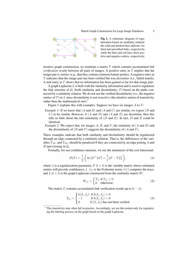
Fig. 1. A schematic diagram of regu-larization based on similarity relation:the solid and dashed lines indicate ver-ified and unverified links, respectively,while the blue and red lines show pos-itive and negative entries, respectively.

iterative graph construction, we maintain a matrix T which contains accumulated linkverification results between all pairs of images. A positive entry in T implies that theimage pair is similar (e.g., that they contain common feature points). A negative entry inT indicates that the image pair has been verified but was dissimilar (i.e., failed match).A null entry in T shows that no information has been gained so far for that image pair.

A graph LaplacianL is built with the similarity information and is used to regularizethe link structure of Gt (both similarity and dissimilarity; T ) based on the paths con-nected by a similarity relation. We do not use the verified dissimilarity (i.e., the negativeentries of T ) in L since dissimilarity is not transitive (the intuitive notion of transitivity,rather than the mathematical one).1

Figure 1 explains this with examples. Suppose we have six images A to F :

Example 1: If we know that (A and B) and (A and C) are similar, we expect (B andC) to be similar. However, if (A and D) and (A and E) are dissimilar, then thistells us little about the (dis-)similarity of (D and E). In fact, D and E could beidentical.

Example 2: We expect that, for images A, B, and F , the similarity of (A and B) andthe dissimilarity of (B and F ) suggests the dissimilarity of (A and F ).

These examples indicate that both similarity and dissimilarity should be regularizedthrough an edge connected by a similarity relation. That is, the differences of the vari-ables TAC and TBC should be penalized if they are connected by an edge joiningA andB and existing in Gt.

Formally, for our confidence measure, we use the minimizer of the cost functional:

O(F ) = 1

2

(λtr[F>LF ] +

1

l‖F − T‖2F

), (1)

where λ is a regularization parameter, F (l × l) is the variable matrix whose estimatedentries will provide confidences, ‖ · ‖F is the Frobenius norm, tr[·] computes the trace,and L (l × l) is the graph Laplacian constructed from the similarity matrix W :

Wij =

{Tij if Tij > 00 otherwise. (2)

The matrix T contains accumulated link verification results up to (t− 1):

Tij =

k(Ii, Ij) if k(Ii, Ij) > 0−1 if k(Ii, Ij) = 00 if (Ii, Ij) has not been verified.

(3)

1 This transitivity may often fail in practice. Accordingly, we use this notion only for regulariz-ing the labeling process on the graph based on the graph Laplacian.


where k(I, J) encodes the results of verification for a pair (I, J). k(·, ·) is 0 when ver-ification fails and is positive otherwise: If verification of (I, J) produces a strength orscore, then k(I, J) is assigned with that specific value. Otherwise, 1 is assigned, indi-cating successful verification. Section 3.3 shows an example of k(·, ·). If the candidatepair (Ii, Ij) do not pass through the filtering phase, we assign−1 to Tij . The minimizerof Eq. 1 can be easily found by solving a set of linear equations:

(λlL+ I)F = T. (4)

We obtain the final confidences by symmetrizing the results (i.e., F ← (F + F>)/2).

3.2 Discussion

Image Webs The most related algorithm to our proposed incremental constructionmethod is Image Webs [3]. Similar to our algorithm, Image Webs builds a graph Lapla-cian and assigns a corresponding score to each unverified edge. This score is used togenerate link candidates. Importantly, the Image Webs edge-ordering criterion is notthe likelihood of being a potential link, which is in explicit contrast with our algorithm:In Image Webs, the objective of link prediction is to maximize algebraic connectivity.Specifically, the score for an edge is calculated from the difference between correspond-ing entries of the Fiedler vector for the nodes it joins. Since the Fiedler vector representsa continuous approximation of the discrete cluster indices in spectral clustering, a largedifference in Fiedler vector entries indicates the possibility of entries being containedin different clusters. As such, these edges are least supported by the context and areunlikely to be real edges. This observation is further supported by our experiments (seeSec. 4). While algebraic connectivity may be useful in analyzing the global structure ofthe match graph [3], we believe it not desirable for the intuitive objective of establishingas many relevant connections as possible between images.

Incremental graph construction phase as link prediction Our problem can be re-garded as a special instance of the more general link prediction problem where onepredicts existences and corresponding properties of links among a set of nodes. Thisis one of the main problems in data mining research, especially in the context of webconnectivity analysis. The use of the graph Laplacian and related methods includingdiffusion kernels, local random walks, etc.2 have already been demonstrated to be veryeffective in this context [17–20]. Our algorithm is different from many of these algo-rithms because our formulation directly uses the links as variables rather than indirectlyclassifying (or clustering) nodes and inferring the properties of links based on the ho-mogeneity of their joined nodes (Eq. 1). In this way, we can systematically exploitdissimilarity as well as similarity information.

From this perspective, a closely related algorithm is proposed by Kunegis et al. [19].They construct a signed Laplacian matrix which includes both similarity (positive en-tries) and dissimilarity (negative entries) information:

L = D −A, (5)2 As l → ∞, the graph Laplacian converges to the Laplacian-Beltrami operator which is the

generator of the diffusion process on a manifold.


where A is the signed similarity matrix (which is equivalent to T in Eq. 1) which in-cludes both positive and negative entries and D is the diagonal matrix given by:

Dii =∑j

|Tij |. (6)

Using this matrix, a positive definite kernel matrix K can be constructed:

K = (I + λLL)−1, (7)

where λL is the regularization parameter such that Kij represents the similarity of thei-th and j-th nodes. This can be used in predicting the existence of potential links: thelarge value of Kij suggests the existence of a link between the i-th and j-th nodes,similarly to the matrix F produced by our algorithm. The authors have demonstratedthat this algorithm is superior to several existing graph Laplacian-based link predictionalgorithms [19]. In the experiments (Sec. 4), we demonstrate that the performance of ouralgorithm is superior to their signed graph Laplacian-based algorithm. Our algorithm isgeneric and can also be applied to general link prediction problems.

The objective (Eq. 1) is sufficient for the classification setting, i.e., to classify eachlink into one of two classes of ‘similar’ and ‘dissimilar’. For a general regression setting(which we do not pursue in this paper), one has to modify the objective such that thetentative assignments of properties (assigned to ‘0’) to unexamined links does not affectthe training error:

O(F ) = 1

2

(λtr[F>LF ] +

1

l‖I′. ∗ (F − T )‖2F

), (8)

where I′ is a matrix with I′ij = 1 if the pair (Ii, Ij) is labeled and zero otherwise; and.∗ represents an element-wise multiplication.

Application specific densification While our criterion for densifying the graph is ob-jective and measurable, it may have to be modified to specifically fit other applications.For instance, in some cases, it might be more desirable to connect a pair of nodes whichhave lower connectivity rather than nodes which already are strongly connected [3]. Wepresent such a modified algorithm for this case in the supplementary material.3

Exploiting sparsity Our algorithm can take advantage of sparsity, especially in con-structing the graph Laplacian L. When the match graph is disconnected due to sparsityeither inherent in the database or caused by a lack of verified links, individual compo-nents can be considered separately. In this case, the negative entries of T connectingdifferent partitions can be neglected: within a component, the results obtained by solv-ing Eq. 4 are identical to those obtained by solving the corresponding system on theentire graph. However, in practice, instead of solving each sub-system, we randomlyselect one connected sub-graph and make predictions only within this graph.

3 We do not evaluate this algorithm since it is difficult to construct an objective criteria.


One computational benefit of Eq. 4 is that its solution can be computed completelyindependently for each column of T . As such, for large-scale partition cases, this canbe performed in multi-processor and multi-memory environments.

Error identification The function k(·, ·) in Eq. 3 may be erroneous in general. Forinstance, 3D geometry-based matching (see Sec. 3.3) may fail, and so there are caseswhere an incorrect link is mistakenly supported by a non-negligible number of featurecorrespondences. The predicted link confidences can also be used to identify potentialmatching mistakes that can subsequently be examined by human operators.

We use the confidence measure (Eq. 1) to re-assign the weights of existing links, i.e.,to replace k(Ii, Ij) with Fij . The links with the largest decrease in link weight becomecandidates for verification. Our preliminary experiments suggested that the best use ofthis approach is to enumerate the nodes which have degree higher than a threshold Td(which is fixed at 5) and to verify each such node in the first several candidates. Thedetails of this experimental setting are described in Sec. 4.

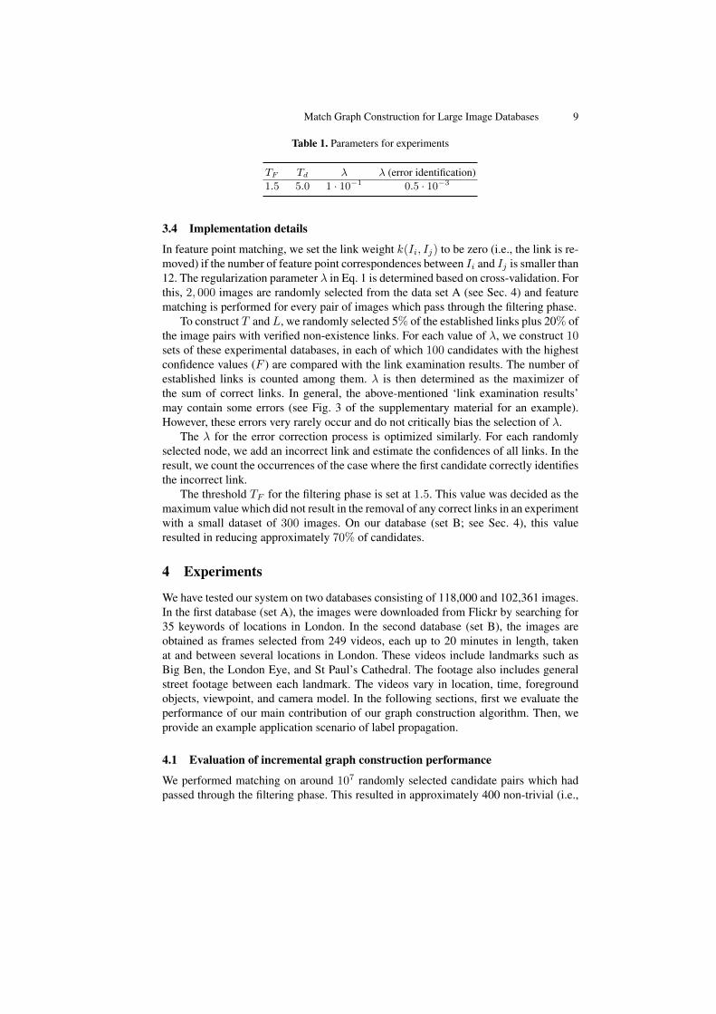
The graph construction step parameters are optimized by performing cross-validationon a small data set. Table 1 summarizes the optimized parameters. See supplementarymaterial for more options for error correction.

3.3 Graph construction with 3D geometry-based matching

While our graph construction technique can be used with any type of image matchingalgorithm, to demonstrate our approach we implement our two-phase graph construc-tion specifically with 3D geometry-based matching, as follows:

1) Filtering phase Each frame is represented with a histogram of a bag of words [21].For each image, the corresponding candidates are the images with distances smallerthan a given threshold TF . We use the spatial pyramid matching kernel [22] as aninverse distance measure.

2) Incremental graph construction phase To match image pairs, we extract SIFT fea-tures [21] from each image. Then, for a given pair of images, RANSAC estimatesfeature correspondences that are most consistent according to the fundamental ma-trix, similar to other related methods [10, 3, 2].

In Eq. 3, k(·, ·) ∈ [0, 1] is the normalized feature correspondence measure given as:

k(Ii, Ij) =2|M(Ii, Ij)||S(Ii)|+ |S(Ij)|

, (9)

where S(I) andM(I, J) are the set of features (SIFT descriptors) calculated fromimage I and the set of features matches for images I and J , respectively. To ensurethat the numbers of SIFT descriptors extracted from any pair of images is compa-rable, all images are scaled to identical heights (540 pixels).4 Intuitively, k(I, J) isclose to 1 when two images I and J contain common features and are similar.

4 Even though the SIFT detectors are theoretically scale invariant, the corresponding implemen-tation is typically scale-dependent. It is common to limit the lowest scale of local extrema inSIFT detection to make the algorithm robust against noise.


Table 1. Parameters for experiments

TF Td λ λ (error identification)1.5 5.0 1 · 10−1 0.5 · 10−3

3.4 Implementation details

In feature point matching, we set the link weight k(Ii, Ij) to be zero (i.e., the link is re-moved) if the number of feature point correspondences between Ii and Ij is smaller than12. The regularization parameter λ in Eq. 1 is determined based on cross-validation. Forthis, 2, 000 images are randomly selected from the data set A (see Sec. 4) and featurematching is performed for every pair of images which pass through the filtering phase.

To construct T and L, we randomly selected 5% of the established links plus 20% ofthe image pairs with verified non-existence links. For each value of λ, we construct 10sets of these experimental databases, in each of which 100 candidates with the highestconfidence values (F ) are compared with the link examination results. The number ofestablished links is counted among them. λ is then determined as the maximizer ofthe sum of correct links. In general, the above-mentioned ‘link examination results’may contain some errors (see Fig. 3 of the supplementary material for an example).However, these errors very rarely occur and do not critically bias the selection of λ.

The λ for the error correction process is optimized similarly. For each randomlyselected node, we add an incorrect link and estimate the confidences of all links. In theresult, we count the occurrences of the case where the first candidate correctly identifiesthe incorrect link.

The threshold TF for the filtering phase is set at 1.5. This value was decided as themaximum value which did not result in the removal of any correct links in an experimentwith a small dataset of 300 images. On our database (set B; see Sec. 4), this valueresulted in reducing approximately 70% of candidates.

4 Experiments

We have tested our system on two databases consisting of 118,000 and 102,361 images.In the first database (set A), the images were downloaded from Flickr by searching for35 keywords of locations in London. In the second database (set B), the images areobtained as frames selected from 249 videos, each up to 20 minutes in length, takenat and between several locations in London. These videos include landmarks such asBig Ben, the London Eye, and St Paul’s Cathedral. The footage also includes generalstreet footage between each landmark. The videos vary in location, time, foregroundobjects, viewpoint, and camera model. In the following sections, first we evaluate theperformance of our main contribution of our graph construction algorithm. Then, weprovide an example application scenario of label propagation.

4.1 Evaluation of incremental graph construction performance

We performed matching on around 107 randomly selected candidate pairs which hadpassed through the filtering phase. This resulted in approximately 400 non-trivial (i.e.,


size larger than 1) subgraphs for set A, and 2000 for set B. Set B has a much highernumber of non-trivial subgraphs since the individual images are sampled densely fromvideos and so it has high connectivity. Many of the images in set A do not correspond toany spatial landmarks (e.g., someone’s face) and are not connected to any other images,so set A is very sparse. The average size of non-trivial subgraphs was around 4 (set A)and 15 (set B) while some subgraphs were several thousand large.

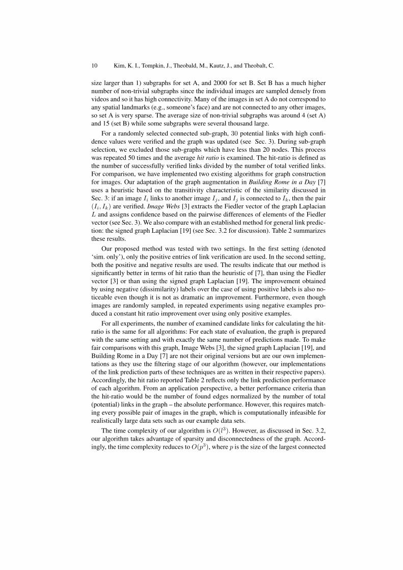
For a randomly selected connected sub-graph, 30 potential links with high confi-dence values were verified and the graph was updated (see Sec. 3). During sub-graphselection, we excluded those sub-graphs which have less than 20 nodes. This processwas repeated 50 times and the average hit ratio is examined. The hit-ratio is defined asthe number of successfully verified links divided by the number of total verified links.For comparison, we have implemented two existing algorithms for graph constructionfor images. Our adaptation of the graph augmentation in Building Rome in a Day [7]uses a heuristic based on the transitivity characteristic of the similarity discussed inSec. 3: if an image Ii links to another image Ij , and Ij is connected to Ik, then the pair(Ii, Ik) are verified. Image Webs [3] extracts the Fiedler vector of the graph LaplacianL and assigns confidence based on the pairwise differences of elements of the Fiedlervector (see Sec. 3). We also compare with an established method for general link predic-tion: the signed graph Laplacian [19] (see Sec. 3.2 for discussion). Table 2 summarizesthese results.

Our proposed method was tested with two settings. In the first setting (denoted‘sim. only’), only the positive entries of link verification are used. In the second setting,both the positive and negative results are used. The results indicate that our method issignificantly better in terms of hit ratio than the heuristic of [7], than using the Fiedlervector [3] or than using the signed graph Laplacian [19]. The improvement obtainedby using negative (dissimilarity) labels over the case of using positive labels is also no-ticeable even though it is not as dramatic an improvement. Furthermore, even thoughimages are randomly sampled, in repeated experiments using negative examples pro-duced a constant hit ratio improvement over using only positive examples.

For all experiments, the number of examined candidate links for calculating the hit-ratio is the same for all algorithms: For each state of evaluation, the graph is preparedwith the same setting and with exactly the same number of predictions made. To makefair comparisons with this graph, Image Webs [3], the signed graph Laplacian [19], andBuilding Rome in a Day [7] are not their original versions but are our own implemen-tations as they use the filtering stage of our algorithm (however, our implementationsof the link prediction parts of these techniques are as written in their respective papers).Accordingly, the hit ratio reported Table 2 reflects only the link prediction performanceof each algorithm. From an application perspective, a better performance criteria thanthe hit-ratio would be the number of found edges normalized by the number of total(potential) links in the graph – the absolute performance. However, this requires match-ing every possible pair of images in the graph, which is computationally infeasible forrealistically large data sets such as our example data sets.

The time complexity of our algorithm is O(l3). However, as discussed in Sec. 3.2,our algorithm takes advantage of sparsity and disconnectedness of the graph. Accord-ingly, the time complexity reduces toO(p3), where p is the size of the largest connected


Table 2. Hit ratios of different link prediction algorithms.

AlgorithmHit ratio

Set A Set B

Image Webs [3] 0.25 0.12Random selection 0.32 0.17Signed graph Laplacian [19] 0.35 0.46Building Rome in a Day [7] 0.49 0.82Proposed method (sim. only) 0.58 0.94Proposed method 0.60 0.97

Table 3. Hit ratios of the first 3 candidates for link error identification.

Candidates 1st 2nd 3rd

Cumulative hit ratio 0.94 0.99 1.00

sub-graph. As such, this theoretical complexity of O(l3) almost never occurs in prac-tice. In experiments, we have almost linear complexity since the individual sub-graphsare sparse. Even for the largest sub-graph (order of thousands), our prediction algorithmtook on average 0.78 second The times taken for Image Webs and Building Rome ina Day were 0.13 and 0.03 second, respectively. The prediction time of our algorithmis longer than that of other algorithms; however, since currently the main bottleneckof these algorithms is the matching stage, this is not a problem. Given that, our wholealgorithm achieves higher connectivity than other algorithms for a given fixed amountof computation time.

We have also evaluated the performance of our link error identification. Since linkerror is very rare, it is hard to evaluate performance systematically. To facilitate eval-uation, we prepared a small dataset of 3, 000 images from set B and built a groundtruth link verification set by exhaustively performing pairwise matching. Then, for eachrandomly selected 500 nodes, we randomly added an ‘incorrect’ link and computed thehit-ratio within the first 3 candidates suggested by our algorithm. Numbers of candidatesranged from 5 (the minimum degree which invokes the error identification process) tohundreds, while the average number of candidates is 18.51. Table 3 summarizes theresults showing that we can very accurately identify erroneous links.

4.2 Application: label propagation in images and videos

In this section, we show the example application of label propagation (LP). This ap-plication requires a graph structure to be constructed from an image database, and hereour algorithm provides this structure.

Our supplementary material contains additional information on 1) active label ac-quisition and how we can provide label suggestions, 2) how new images can be addedto existing graphs in cases where the database is not fixed a priori, and 3) additionalsteps required for processing videos instead of images.


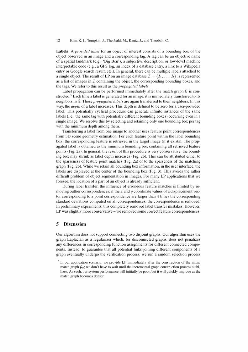
Labels A provided label for an object of interest consists of a bounding box of theobject observed in an image and a corresponding tag. A tag can be an objective nameof a spatial landmark (e.g., ‘Big Ben’), a subjective description, or low-level machineinterpretable code (e.g., a GPS log, an index of a database entry, a link to a Wikipediaentry or Google search result, etc.). In general, there can be multiple labels attached toa single object. The result of LP on an image database I = {I1, . . . , Il} is representedas a list of images in I containing the object, the corresponding bounding boxes, andthe tags. We refer to this result as the propagated labels.

Label propagation can be performed immediately after the match graph G is con-structed.5 Each time a label is generated for an image, it is immediately transferred to itsneighbors in G. Those propagated labels are again transferred to their neighbors. In thisway, the depth of a label increases. This depth is defined to be zero for a user-providedlabel. This potentially cyclical procedure can generate infinite instances of the samelabels (i.e., the same tag with potentially different bounding boxes) occurring even in asingle image. We resolve this by selecting and retaining only one bounding box per tagwith the minimum depth among them.

Transferring a label from one image to another uses feature point correspondencesfrom 3D scene geometry estimation. For each feature point within the label boundingbox, the corresponding feature is retrieved in the target image (if it exists). The prop-agated label is obtained as the minimum bounding box containing all retrieved featurepoints (Fig. 2a). In general, the result of this procedure is very conservative: the bound-ing box may shrink as label depth increases (Fig. 2b). This can be attributed either tothe sparseness of feature point matches (Fig. 2a) or to the sparseness of the matchinggraph (Fig. 2b). While we retain all bounding box information, in the user interface, thelabels are displayed at the center of the bounding box (Fig. 3). This avoids the ratherdifficult problem of object segmentation in images. For many LP applications that weforesee, the location of a part of an object is already sufficient.

During label transfer, the influence of erroneous feature matches is limited by re-moving outlier correspondences: if the x and y coordinate values of a displacement vec-tor corresponding to a point correspondence are larger than 4 times the correspondingstandard deviations computed on all correspondences, the correspondence is removed.In preliminary experiments, this completely removed label transfer mistakes. However,LP was slightly more conservative – we removed some correct feature correspondences.

5 Discussion

Our algorithm does not support connecting two disjoint graphs: Our algorithm uses thegraph Laplacian as a regularizer which, for disconnected graphs, does not penalizesany differences in corresponding function assignments for different connected compo-nents. Instead, to guarantee that all potential links joining different components of agraph eventually undergo the verification process, we run a random selection process

5 In our application scenario, we provide LP immediately after the construction of the initialmatch graph G0; we don’t have to wait until the incremental graph construction process stabi-lizes. As such, our system performance will initially be poor, but it will quickly improve as thematch graph becomes denser.


“London eye” A B

C

(a) (b)

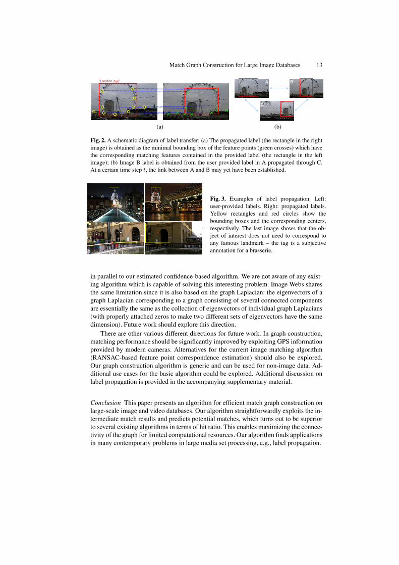
Fig. 2. A schematic diagram of label transfer: (a) The propagated label (the rectangle in the rightimage) is obtained as the minimal bounding box of the feature points (green crosses) which havethe corresponding matching features contained in the provided label (the rectangle in the leftimage); (b) Image B label is obtained from the user provided label in A propagated through C.At a certain time step t, the link between A and B may yet have been established.

Fig. 3. Examples of label propagation: Left:user-provided labels. Right: propagated labels.Yellow rectangles and red circles show thebounding boxes and the corresponding centers,respectively. The last image shows that the ob-ject of interest does not need to correspond toany famous landmark – the tag is a subjectiveannotation for a brasserie.

in parallel to our estimated confidence-based algorithm. We are not aware of any exist-ing algorithm which is capable of solving this interesting problem. Image Webs sharesthe same limitation since it is also based on the graph Laplacian: the eigenvectors of agraph Laplacian corresponding to a graph consisting of several connected componentsare essentially the same as the collection of eigenvectors of individual graph Laplacians(with properly attached zeros to make two different sets of eigenvectors have the samedimension). Future work should explore this direction.

There are other various different directions for future work. In graph construction,matching performance should be significantly improved by exploiting GPS informationprovided by modern cameras. Alternatives for the current image matching algorithm(RANSAC-based feature point correspondence estimation) should also be explored.Our graph construction algorithm is generic and can be used for non-image data. Ad-ditional use cases for the basic algorithm could be explored. Additional discussion onlabel propagation is provided in the accompanying supplementary material.

Conclusion This paper presents an algorithm for efficient match graph construction onlarge-scale image and video databases. Our algorithm straightforwardly exploits the in-termediate match results and predicts potential matches, which turns out to be superiorto several existing algorithms in terms of hit ratio. This enables maximizing the connec-tivity of the graph for limited computational resources. Our algorithm finds applicationsin many contemporary problems in large media set processing, e.g., label propagation.


Acknowledgement We thank Nils Hasler for proof reading.

References

1. Snavely, N., Seitz, S.M., Szeliski, R.: Photo tourism: exploring photo collections in 3D.ACM TOG (Proc. SIGGRAPH) 25 (2006) 835–846

2. Raguram, R., Wu, C., Frahm, J.M., Lazebnik, S.: Modeling and recognition of landmarkimage collections using iconic scene graphs. IJCV (to appear)

3. Heath, K., Gelfand, N., Ovsjanikov, M., Aanjaneya, M., Guibas, L.J.: Image webs: comput-ing and exploiting connectivity in image collections. In: Proc. IEEE CVPR. (2010) 3432–3439

4. Gammeter, S., Bossard, L., Quack, T., Gool, L.V.: I know what you did last summer: object-level auto-annotation of holiday snaps. In: Proc. ICCV. (2009) 614–621

5. Zheng, Y.T., Zhao, M., Song, Y., Adam, H., Buddemeier, U., Bissacco, A., Brucher, F., Chua,T.S., Neven, H.: Tour the world: building a web-scale landmark recognition engine. In: Proc.IEEE CVPR. (2009) 1085–1092

6. Kennedy, L., Naaman, M.: Generating diverse and representative image search results forlandmarks. In: Proc. WWW. (2008) 297–306

7. Agarwal, S., Snavely, N., Simon, I., Seitz, S.M., Szeliski, R.: Building Rome in a day. In:Proc. ICCV. (2009)

8. Tompkin, J., Kim, K.I., Kautz, J., Theobalt, C.: Videoscapes: exploring sparse, unstructuredvideo collections. ACM TOG (Proc. SIGGRAPH) (2012) 68:1–12

9. Sivic, J., Zisserman, A.: Video Google: A text retrieval approach to object matching invideos. In: Proc. ICCV. (2003) 1470–1477

10. Hartley, R.I., Zisserman, A.: Multiple View Geometry in Computer Vision. 2nd edn. Cam-bridge University Press (2004)

11. Philbin, J., Sivic, J., Zisserman, A.: Geometric latent Dirichlet allocation on a matchinggraph for large-scale image datasets. IJCV 95(2) (2011) 138–153

12. Weyand, T., Leibe, B.: Discovering favorite views of popular places with iconoid shift. In:Proc. ICCV. (to appear)

13. Hays, J., Efros, A.A.: IM2GPS: estimating geographic information from a single image. In:Proc. IEEE CVPR. (2008) 1–8

14. Kleban, J., Moxley, E., Xu, J., Manjunath, B.S.: Global annotation on georeferenced pho-tographs. In: Proc. CIVR. (2009) 1–8

15. Serdyukov, P., Murdock, V., van Zwol, R.: Placing flickr photos on a map. In: Proc. SIGIR.(2009) 484–491

16. Crandall, D.J., Backstrom, L., Huttenlocher, D., Kleinberg, J.: Mapping the world’s photos.In: Proc. WWW. (2009) 761–770

17. Kunegis, J., Lommatzsch, A.: Learning spectral graph transformations for link prediction.In: Proc. ICML. (2009) 561–568

18. Backstrom, L., Leskovec, J.: Supervised random walks: predicting and recommending linksin social networks. In: Proc. WSDM. (2011) 635–644

19. Kunegis, J., Schmidt, S., Lommatzsch, A., Lerner, J., Luca, E.W., Albayrak, S.: Spectralanalysis of signed graphs for clustering, prediction and visualization. In: Proc. ICDM. (2010)559–570

20. Lu, L., Zhou, T.: Link prediction in complex networks: a survey. arXiv:1010.0725v1 (2011)21. Lowe, D.G.: Distinctive image features from scale-invariant keypoints. IJCV 60(2) (2004)

91–11022. Lazebnik, S., Schmid, C., Ponce., J.: Beyond bags of features: spatial pyramid matching for

recognizing natural scene categories. In: Proc. IEEE CVPR. (2006) 2169–2178

Documents

Match Graph Construction for Large Image Databases