Material Point Method Calculations with Explicit Cracksguilkey/MPMPubs/NairnMPMCracks.pdf · Material Point Method Calculations with Explicit Cracks ... periments show it gets good

Copyright c© 2003 Tech Science Press CMES, vol.4, no.6, pp.649-663, 2003

Material Point Method Calculations with Explicit Cracks

J. A. NAIRN 1

Abstract: A new algorithm is described which extendsthe material point method (MPM) to allow explicit crackswithin the model material. Conventional MPM enforcesvelocity and displacement continuity through its back-ground grid. This approach is incompatible with crackswhich are displacement and velocity discontinuities. Byallowing multiple velocity fields at special nodes nearcracks, the new method (called CRAMP) can modelcracks. The results provide an “exact” MPM analysis forcracks. Comparison to finite element analysis and to ex-periments show it gets good results for crack problems.The intersection of crack surfaces is prevented by imple-menting a crack contact scheme. Crack contact can bemodeled using stick or sliding with friction. All resultsare two dimensional, but the methods can be extended tothree dimensional problems.

keyword: Material point method, cracks, fracture, nu-merical methods, contact

1 Introduction

The material point method (MPM) has recently been de-veloped as a numerical method for solving problems indynamic solid mechanics [Sulsky, Chen, and Schreyer(1994), Sulsky, Zhou, and Schreyer (1995), Sulsky andSchreyer (1996), Zhou (1998)]. In MPM, a solid body isdiscretized into a collection of points much like a com-puter image is represented by pixels. As the dynamicanalysis proceeds, the solution is tracked on the mate-rial points by updating all required properties such as po-sition, velocity, acceleration, stress state,etc.. At eachtime step, the particle information is extrapolated to abackground grid which serves as a calculational tool tosolve the equations of motions. Once the equations aresolved, the grid-based solution is used to update all parti-cle properties. This combination of Lagrangian and Eu-lerian methods has proven useful for solving solid me-

1Material Science and Engineering, University of Utah, Salt LakeCity, Utah 84112, USA

chanics problems including those with large deforma-tions or rotations and involving materials with history de-pendent properties such as plasticity or viscoelasticity ef-fects [Sulsky, Chen, and Schreyer (1994), Sulsky, Zhou,and Schreyer (1995), Sulsky and Schreyer (1996), Zhou(1998)]. MPM is amendable to parallel computation[Parker (2002)], implicit integration methods [Guilkeyand Weiss (2002)], and alternative interpolation schemesthat improve accuracy [Bardenhagen and Kober (2003)].

Although MPM uses a background grid and is frequentlycompared to finite element methods, a new derivationor MPM [Bardenhagen and Kober (2003)] presents itas a Petrov-Galerkin method that has similarities withmeshless methods such as Element-Free Galerkin (EFG)methods [Belytschko, Lu, and Gu (1994)] and Meshless-Local Petrov-Galerkin (MLPG) methods [Atluri andShen (2002a), Atluri and Shen (2002b), Atluri and Zhu(1998)]. The “meshless” aspect of MPM, despite the useof a grid, derives from the fact that the body and the solu-tion are described on the particles while the grid is usedsolely for calculations. The body can translate throughthe grid. Furthermore the grid can be discarded each timestep and redrawn which makes MPM suitable to adaptivemesh methods. It is essential for any extension to MPM,such as presented here, to preserve the separation be-tween the grid and the particles. MPM, EFG, and MLPGdiffer in their methods used to derive shape functions andin their selection of test functions during numerical im-plementation [Bardenhagen and Kober (2003), Atluri andShen (2002a)].

One potential application of MPM is as a tool in dynamicfracture modeling. It was recently shown that MPM canaccurately calculate fracture parameters such as energyrelease rate [Tan and Nairn (2002)], but those resultswere for a crack at a symmetry plane and thus the crackcould be described by symmetry conditions alone. Con-ventional MPM is not capable of handling explicit, inter-nal cracks. The problem is that conventional MPM meth-ods extrapolate particle information to a single velocity

650 Copyright c© 2003 Tech Science Press CMES, vol.4, no.6, pp.649-663, 2003

field on the background grid. A property of the back-ground grid, which is analogous to finite element analy-sis grids, is that all displacements in the single velocityfield are continuous. Because representation of cracksrequires displacement discontinuities, MPM can not rep-resent cracks.

This paper describes a modified material point method la-beled as CRAMP for ”CRAcks” with ”Material Points.”The following list gives the essential differences betweenCRAMP and conventional MPM:

1. Cracks are described in 2D as a series of line seg-ments. The end-points of the line segments can beadditional mass-less particles to make it easy to addcrack descriptions to standard MPM data structures.

2. Each node in the background grid is allowed to havemultiple velocity fields. If the node is far from anycrack, the node will have a single velocity field asin conventional MPM. For nodes near a crack, how-ever, each node will have separate velocity fields forinformation interpolated from particles on oppositesides of a crack.

3. Most calculations in the MPM algorithm needed tobe adjusted to account for the possibility that a par-ticular node might have multiple velocity fields.

4. When nodes have separate velocity fields and dis-placement continuities, it is possible for the twosides of the crack to cross over each other. To pre-vent non-physical crossing, all calculations at nodeswith multiple velocity fields must implement con-tact methods. The algorithm in this paper can modelcrack contact by stick or by sliding with friction.

5. A modified scheme for updating stresses and strainswas added which appears to improve energy calcu-lations. An important application of crack calcula-tions is to do fracture predictions. Because fracturework requires accurate energy calculations, it wasimportant to optimize the MPM energy results. Thislast correction can be applied to conventional MPMas well as to CRAMP.

All results in this paper are for 2D calculations. In mostcases, the extension to 3D is simple and obvious. The oneexception is the crack description. In 3D, the crack needsto be described by connected surfaces instead of line seg-ments. The algorithm presented here does stress analysis

calculations for existing, internal cracks. The subject ofevaluating fracture parameters at crack tips and predict-ing crack propagation will be in future work. The crackdescription used, however, is very flexible. It is a triv-ial matter to extend the crack during a dynamic analysisonce the harder problem of deciding when and where toextend the crack has been solved. Finally, the CRAMPalgorithm is efficient. Comparison between conventionalMPM and CRAMP show the crack calculations to beonly about 10% slower. The most time consuming partof the CRAMP algorithm is determining which particlesinterpolate to which velocity field at each node.

2 MPM With Explicit Cracks — CRAMP

This section describes the CRAMP algorithm for includ-ing explicit cracks in MPM calculations. The features ofthe algorithm are given here; the full algorithm is pro-vided in the Appendix. The first task is to describe theinternal cracks. One simple way to introduce displace-ment discontinuities into MPM would be to introducecracks in the background grid. Although this approachcan handle certain problems, it severely limits the flexi-bility of MPM. The background grid is supposed to serveas a calculational tool and not as a device to carry infor-mation about the solution or about the solid. It wouldalso be difficult or impossible to translate the crack alongwith the body during large deformation calculations. InCRAMP, the crack is instead described as a series of linesegments. For compatibility with MPM data structures,the endpoints of the line segments are massless materialpoints. By translating the crack segments along with thesolution, it is possible to track cracks in moving bodies.A problem can contain any number of cracks.

2.1 Multiple Velocity Fields

The influence of cracks on the MPM solution is thatthey influence the velocity fields at some nodes in thebackground grid. In conventional MPM, the first step inthe algorithm is to extrapolate the particle momenta andmasses to the background grid. The equations are [Sul-sky, Zhou, and Schreyer (1995)]:

pki =

np

∑p=1

mpvkpSk

i,p mDki =

np

∑p=1

mpSki,p (1)

wherepki is nodal momentum,vk

p is particle velocity,mp

is particle mass,Ski,p is the shape function for nodei eval-

MPM Calculations with Explicit Cracks 651

uated at the current position of particlep, and mDki is

the nodal mass in the lumped (or diagonal) mass matrix.The superscriptk indicates these terms apply to thekth

MPM step. In this approach, each nodal point has a sin-gle momentum and displacement discontinuities are notallowed. To allow displacement discontinuities, CRAMPallows each node to have three types of velocity fields -one for particles on the same side of all cracks as thenode (0), one for particles above a crack relative to thenode (1), and one for particles below a crack relative tothe node (2). The first step in crack calculations is thus toexamine each particle-node combination (with non-zeroshape function) and determine the appropriate velocityfield denoted by

ν(p, i) = 0, 1, or 2 (2)

This determination is done by a line-crossing algorithm.First, a line is drawn from particlep to nodei. If theline does not cross any crack, the velocity field is 0; if itcrosses a crack from above, the velocity field is 1; if itcrosses a crack from below, the velocity field is 2. Thefield determination is the most time consuming part ofCRAMP and must be done efficiently; an efficient algo-rithm is given in the Appendix. Once the velocity field’sare determined, the modified, initial MPM extrapolationsbecome

pki, j =

np

∑p=1

mpvkpSk

i,pδ j,ν(p,i)

mDki, j =

np

∑p=1

mpSki,pδ j,ν(p,i)

j = 0, 1, 2 (3)

Each node may have one to three velocity fields denotedby index j on pk

i, j and mDki, j . Each velocity field inter-

polates only from particles contributing to that field asdetermined by the Kronecker delta functionδ j,ν(p,i). Al-though three velocity fields are defined, no node shouldever have more that two velocity fields — one each forparticles on the two sides of a crack.

The possible existence of multiple velocity fields carriesthrough the remainder of the algorithm. Each conven-tional MPM calculation must consider all velocity fields.For example, the total nodal forces (with damping) are

f toti, j = f int

i, j + f exti, j −κpk

i, j j = 0, 1, 2 (as needed) (4)

where f inti, j and f ext

i, j are internal and external forces at anode andκ is a damping coefficient. The updated nodal

momenta become

pk′i, j = pk

i, j +∆t f toti, j j = 0, 1, 2 (as needed) (5)

where∆t is the time step. When updating particle posi-tions, velocities, stresses, and strains, the equations onlyuse the velocity field appropriate to each particle/nodepair. For example, updating of position becomes

xk+1p = xk

p +∆tnn

∑i=1

pk′i,ν(p,i)S

ki,p

mDki,ν(p,i)

(6)

Above are some examples of the modified equations; allthe required modifications are detailed in the Appendix.

If the body is translating, all cracks need to translatealong with it. This task is accomplished by calculatingthe center of mass velocity of each node with multiplevelocity fields:

vki,cm =

∑3j=1pk′′

i, jϕi, j

∑3j=1mDk

i, j ϕi, j(7)

whereϕi, j is 1 or 0 depending on whether or not veloc-ity field j is present at nodei. Once all nodal velocitiesare reduced to a single field, the mass-less particles thatdefine the crack can move using standard MPM methodsfor updating particle position.

2.2 Crack Surface Contact

Several times during each MPM step, the nodal momentaand velocities are updated. These updates may occur as aconsequence of boundary conditions or when implement-ing the equations of motion. Whenever the nodal mo-menta change, it is essential to verify that the change cor-responds to a physically allowed change which is definedhere as meaning that opposite sides of cracks do not crossover each other. To prevent non-physical changes, theCRAMP algorithm includes contact methods. The meth-ods are based on the contact methods develop by Barden-hagen [Bardenhagen, Brackbill, and Sulsky (2000), Bar-denhagen, Guilkey, Roessig, Brackbill, Witzel, and Fos-ter (2001)], but there are two key differences. First, themethods in Bardenhagen, Brackbill, and Sulsky (2000)and Bardenhagen, Guilkey, Roessig, Brackbill, Witzel,and Foster (2001) were for contact between dissimilarmaterials; here contact is within the same material but ontwo sides of a crack. Second, their methods used to iden-tify contact did not work well for internal cracks; they


would either identify contact too soon or identify it un-reliably. This section describes the contact methods inCRAMP.

The identification of crack surface contact is basedmostly on nodal volume at crack nodes (i.e., nodes withmultiple velocity fields). The total nodal volume (whichis a nodal area in 2D calculations) is calculated duringeach MPM step using

Vki =

np

∑p=1

VkpSk

i,p (8)

whereVkp is the volume of particlep or an area in 2D

calculations defined by

Vkp = (1+ εk

p,xx)(1+ εkp,yy)

mp

ρptp(9)

whereρp andtp are the density and thickness of the 2Dparticle. Whenever momenta change, the nodal volumesat all nodes with multiple velocity fields are normalizedby the undeformed volume. For regular grids the un-deformed volume is the volume of each element in thebackground grid; for irregular grids, the undeformed vol-ume includes a portion of each element containing thatnode. The relative volume is defined as

Vrel =Vk

i

Vunde fi

(10)

Two critical relative volumes are preselected asVsep(lessthan 1) andVcontact (greater than 1). IfVrel < Vsep,the crack surfaces are assumed to be separated and nochanges in momenta are needed. IfVrel > Vcontact, thecracks surfaces are assumed to be in contact and mo-menta are adjusted as explained below. The regionVsep<Vrel < Vcontact is a gray area and a second method is usedto decide whether or not contact is present.

Several second methods are possible, but the calculationshere used relative velocity of the two crack surfaces [Bar-denhagen, Brackbill, and Sulsky (2000), Bardenhagen,Guilkey, Roessig, Brackbill, Witzel, and Foster (2001)].Once a crack node withVsep<Vrel <Vcontact is found, thevelocities above and below the crack are calculated from

vki,a =

pki,a

mDki,a

vki,b =

pki,b

mDki,b

(11)

wherea andb indicate the velocity fields correspondingto particles above and below the crack. By examining

the angle between the relative velocities and the cracksurface normal, the cracks are assumed to be separated ifthey are moving apart as defined by

(vki,a−vk

i,b) · n≤ 0 (12)

wheren is the crack surface normal. If the crack surfacesare moving towards each other, the cracks are assumedto be in contact and the momenta are adjusted. The cracksurface normal can be calculated earlier in the algorithmduring the line-crossing algorithm. Whenever a line froma particle to a node crosses a crack, the normal to thatcrack segment is saved for that node. The normal at agiven node is the average of all such normal vectors. Thenormal is defined as directed from above the crack to be-low the crack.

Once contact is identified (byVrel > Vcontact or by cracksurfaces moving towards each other), the momenta areadjusted by two alternate methods. The simplest contactmethod is contact bystick conditions. Thestick methodsimply reverts to conventional MPM where the momentaabove and below the crack are set equal to each otherand equal to the center-of-mass momenta. The requiredmomenta changes to implementstickconditions are

∆pki,a =

mDki,apk

i,b−mDki,bpk

i,a

mDki,a +mDk

i,b

∆pki,b =−∆pk

i,a (13)

These changes conserve total momentum.

A frictional sliding contact method follows the approachof Bardenhagen, Guilkey, Roessig, Brackbill, Witzel,and Foster (2001). In physical terms, this method adjuststhe velocity above the crack to be

vki,a = vk

i,a−∆vn(n+µ′ t

)(14)

wheret is a unit normal tangential to the crack surface inthe direction of sliding andµ′ is aneffectivecoefficient offriction defined by

µ′ = min

(µ,

∆vt

∆vn

)(15)

Hereµ is the actual coefficient of friction, and∆vn and∆vt are the components of the relative crack face veloci-ties normal and tangential to the crack:

∆vn =(vk

i,a−vki,b

)· n ∆vt =

(vk

i,a−vki,b

)· t (16)

Whenµ′ reduces to∆vt/∆vn, the surfaces are sticking dueto friction or the velocities are adjusted to equal the cen-ter of mass velocities. Whenµ′ reduces toµ, the contact


is by friction. In the limit of frictionless sliding (µ = 0),µ′ is always zero, the crack surface velocities normalto the surfaces are adjusted to be equal and the tangen-tial velocities remain unchanged. All CRAMP algorithmsteps are in terms of nodal momenta instead of velocities.The above velocity equations in terms of momenta cor-respond to adjusting the momenta above and below thecrack by

∆pki,a =

[(mDk

i,apki,b−mDk

i,bpki,a

mDki,a +mDk

i,b

)· n

](n−µ′ t

)∆pk

i,b = −∆pki,a

(17)wheret is now a unit vector tangential to the crack sur-face that is in the same direction as the crack line seg-ments andµ′ is a signed quantity given by

µ′ =

−µ if

∆vt

∆vn<−µ

+µ if∆vt

∆vn> +µ

∆vt

∆vnotherwise

(18)

Finally, the normal and tangential velocity componentscan be calculated from

∆vn =mDk

i,apki,b−mDk

i,apki,b

mDki,a

· n

∆vt =mDk

i,apki,b−mDk

i,apki,b

mDki,a

· t(19)

One difference between this frictional contact methodand the one in Bardenhagen, Guilkey, Roessig, Brackbill,Witzel, and Foster (2001) is that the same normal is usedfor both crack surfaces (it is defined from the crack linesegments) and thus momentum is exactly conserved. InBardenhagen, Guilkey, Roessig, Brackbill, Witzel, andFoster (2001), the two contacting materials had separatenormal vectors and momentum was only conserved whenthose normals were equal and opposite.

2.3 Modified Method to Update Particle Stresses andStrains

One part of each MPM step involves updating the parti-cle stresses and strains. If this task is not done optimally,there can be numerical difficulties and inaccuracies in en-ergy calculations. Because accurate energy results areessential for fracture calculations, the updating methods

were examined and slightly revised from previous meth-ods in the literature [Sulsky, Chen, and Schreyer (1994),Sulsky, Zhou, and Schreyer (1995), Sulsky and Schreyer(1996), Zhou (1998), Bardenhagen (2002)].

As explained in the appendix, updating the stresses andstrains on the particles involves calculating the strain in-crement for the current step and then using a constitu-tive law to determine the stress increment. The strainincrement is a function of the current strain rate whichis calculated from the current nodal velocities (see Sub-task 2 for updating stresses and strains in the Appendix).There are several alternatives for which nodal velocitiesto use for the updating process. In an early MPM paper[Sulsky, Chen, and Schreyer (1994)], the nodal velocitieswere calculatedafter updating the nodal momenta. Thisapproach, referred to as the “Update Stress Last” or USL,has serious numerical difficulties which are revealed byconsidering a node which interacts with only a single par-ticle. Following through the algorithm in the Appendix,the nodal velocity used for strain rates would at such anode would be

vi = vkp +∆t

(−

σkp ·Gk

i,p

Ski,p

+bp +f kp

mp

)(20)

For simplicity, this analysis only considers a single ve-locity field and ignores damping. Only a single velocityfield is considered, because only one is possible whenthere is only a single particle. As a consequence, all dis-cussion in this section applies to both conventional MPMand to CRAMP. The first term in the brackets causes aproblem. When the one particle is on the opposite side ofthe element from the node, the shape function (Sk

i,p) willapproach zero, but its gradient (Gk

i,p) will not. The firstterm is thus unstable.

There are two solutions to the USL dilemma. The first so-lution was given by Sulsky, Zhou, and Schreyer (1995).Their approach was to adopt a momentum based algo-rithm similar to the approach in the Appendix. It wasnot the use of momentum that improved the algorithm,but rather the way nodal velocities were calculated beforeupdating particle stresses and strains. In their approach,referred to as “Modified Update Stress Last” or MUSL,the updated particle momenta are extrapolated to the grida second time before calculating the nodal velocities (seeTask 6c in the appendix). Tracing a node with a single


particle, the nodal velocities used for strain rates become

vi = vkp +∆t

nn

∑i=1

f toti Sk

i,p

mDki

(21)

Although some nodal masses in the denominator (mDki )

may approach zero, whenever the mass is close the zero,there will be a correspondingSk

i,p identically close to zeroto cancel it out. This approach greatly improves the sta-bility of MPM. An alternate fix is to update strainsbe-fore updating momentum [Bardenhagen (2002)]. In thisapproach, referred to as “Update Stress First” or USF,the nodal velocities (for a single-particle node) used forstrain rates are simply

vi = vkp (22)

which clearly have no numerical difficulties.

MUSL and USF are nearly identical. MUSL finds ve-locities for momenta extrapolated at the end of an MPMstep while USF finds velocities from the same momentaby extrapolating at the beginning of the next time step.The only mathematical difference between these two ap-proaches is the shape functions used in the extrapolation.MUSL usingSk

i,p while USF usesSk+1i,p . In numerous cal-

culations, both give greatly improved energy calculationscompared to USL methods. MUSL tends to slowly dissi-pate energy while USF tends to slowly increase in energy[Bardenhagen (2002)]. This observation leads to an ob-vious compromise which combines MUSL and USF byupdating stresses and strains both before updating nodalmomenta and after updating (and re-extrapolating) nodalmomenta. In this approach, referred to as “Update StressAveraged” or USAVG, the strain increment at each up-dating is divided by 2 to use the two methods equally. Innumerous calculations, MPM results using USAVG con-serves energy nearly exactly. Sample calculations com-paring USAVG to USL, MUSL, and USF are given in thenext section.

3 Results and Discussion

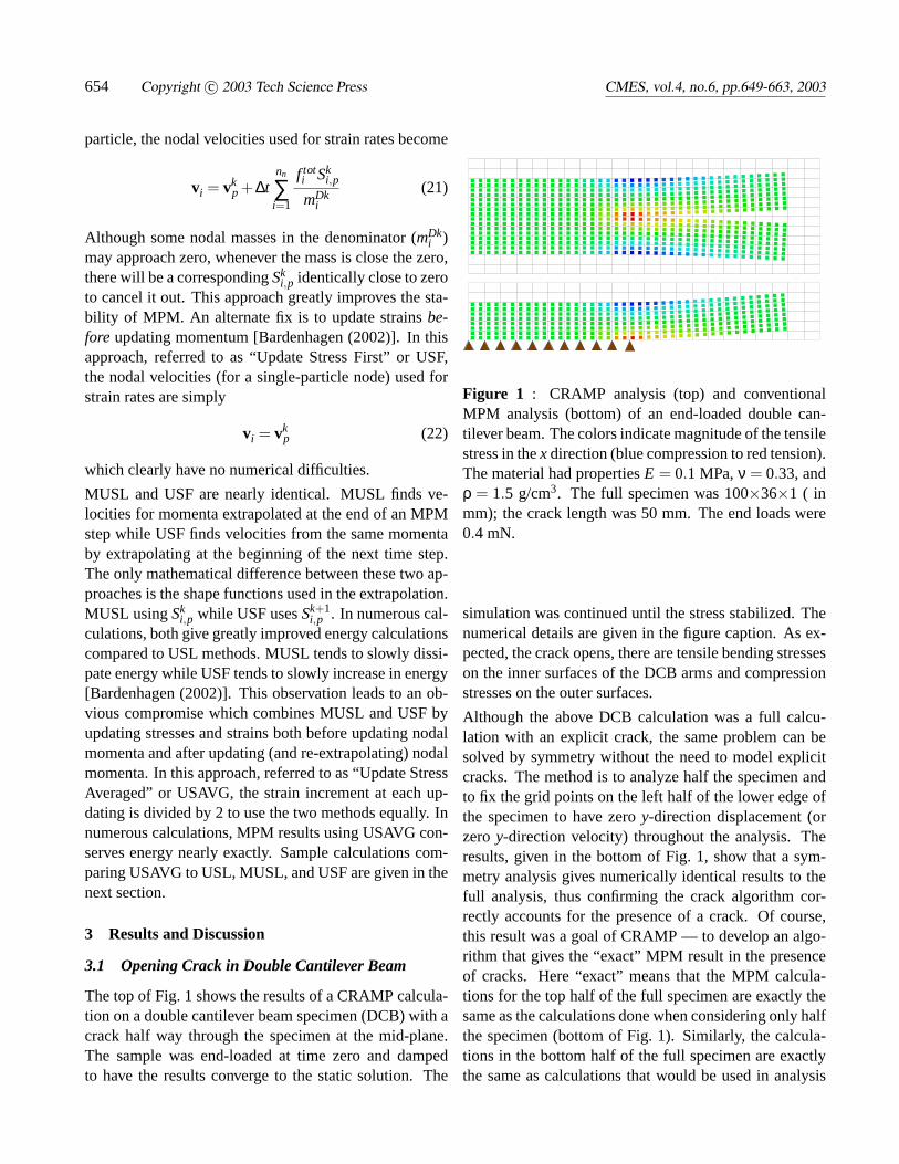
3.1 Opening Crack in Double Cantilever Beam

The top of Fig. 1 shows the results of a CRAMP calcula-tion on a double cantilever beam specimen (DCB) with acrack half way through the specimen at the mid-plane.The sample was end-loaded at time zero and dampedto have the results converge to the static solution. The

Figure 1 : CRAMP analysis (top) and conventionalMPM analysis (bottom) of an end-loaded double can-tilever beam. The colors indicate magnitude of the tensilestress in thex direction (blue compression to red tension).The material had propertiesE = 0.1 MPa,ν = 0.33, andρ = 1.5 g/cm3. The full specimen was 100×36×1 ( inmm); the crack length was 50 mm. The end loads were0.4 mN.

simulation was continued until the stress stabilized. Thenumerical details are given in the figure caption. As ex-pected, the crack opens, there are tensile bending stresseson the inner surfaces of the DCB arms and compressionstresses on the outer surfaces.

Although the above DCB calculation was a full calcu-lation with an explicit crack, the same problem can besolved by symmetry without the need to model explicitcracks. The method is to analyze half the specimen andto fix the grid points on the left half of the lower edge ofthe specimen to have zeroy-direction displacement (orzeroy-direction velocity) throughout the analysis. Theresults, given in the bottom of Fig. 1, show that a sym-metry analysis gives numerically identical results to thefull analysis, thus confirming the crack algorithm cor-rectly accounts for the presence of a crack. Of course,this result was a goal of CRAMP — to develop an algo-rithm that gives the “exact” MPM result in the presenceof cracks. Here “exact” means that the MPM calcula-tions for the top half of the full specimen are exactly thesame as the calculations done when considering only halfthe specimen (bottom of Fig. 1). Similarly, the calcula-tions in the bottom half of the full specimen are exactlythe same as calculations that would be used in analysis


of a lower-half specimen. The complication in a fullspecimen is that both halves need to use the mid-planenodes for normal MPM calculations. This simultaneoususe of the mid-plane nodes is accomplished naturally inthe CRAMP algorithm by those nodes having two veloc-ity fields.

An alternate approach to handling explicit cracks inMPM is to modify the calculations using node-visibilitycriteria. In node-visibility methods, a line is drawn fromeach particle to each node. If that line crosses a crack,than that node no longer influences the calculations forthat particle. Node visibility [Belytschko, Lu, and Gu(1994)] and the related diffraction criteria [Organ, Flem-ing, and Belytschko (1996)] have been the most commonchoices for implementing cracks in EFG [Belytschko andTabbara (1996)] and MLPG [Ching and Batra (2001),Batra and Batra (2002)] methods. Although node visi-bility can also implement cracks in MPM, it leads to lessaccurate results than the CRAMP method. The abovedefinition of “exact” MPM could be rephrased as a “crackpatch” test in which the results of any crack algorithm ap-plied to a symmetric problem with an explicit crack arecompared to a standard analysis with no crack algorithmthat includes the crack by symmetry conditions alone.An algorithm passes the test if the results of the twoanalysis are numerically identical. The CRAMP methodpasses the “crack patch” test while MPM with node vis-ibility does not. Similarly, because node visibility anddiffraction criteria in EFG and MLPG modify the shapefunctions differently than when the crack is defined onlyby symmetry conditions, those methods also would notpass a “crack patch” test.

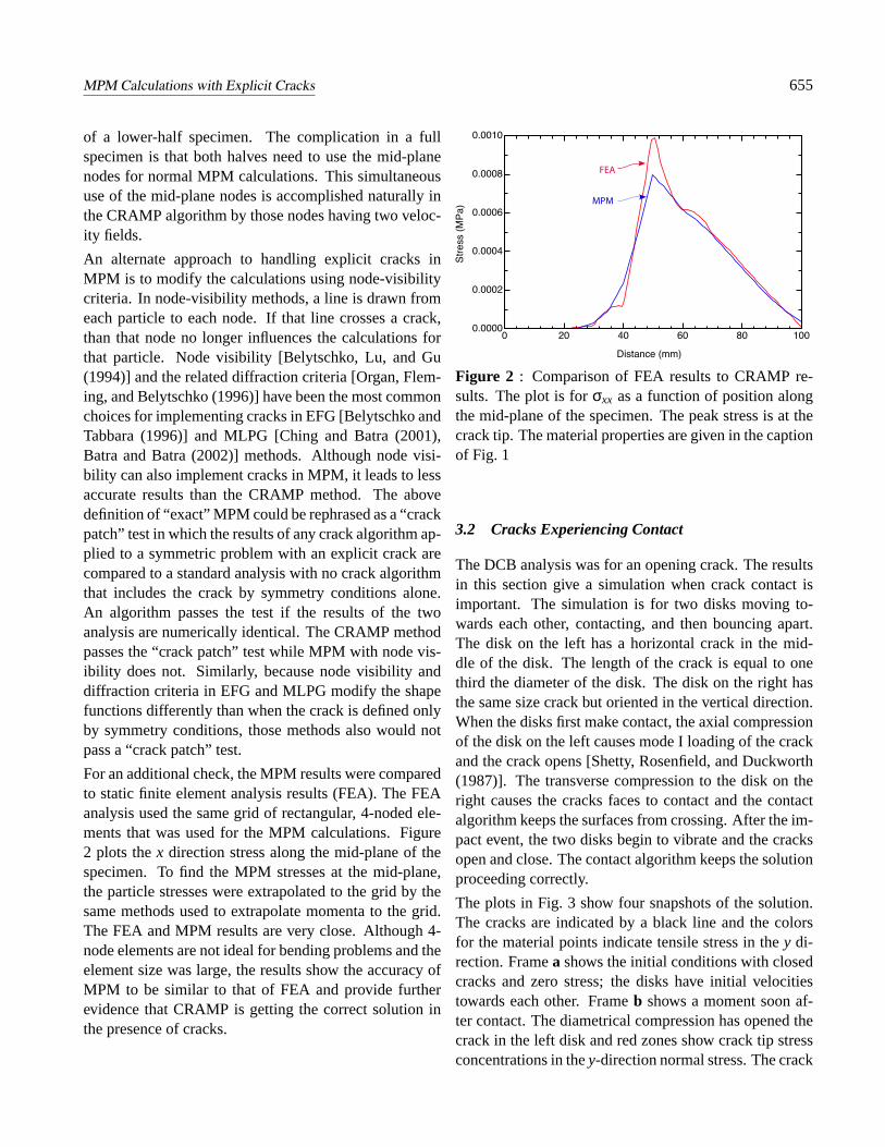
For an additional check, the MPM results were comparedto static finite element analysis results (FEA). The FEAanalysis used the same grid of rectangular, 4-noded ele-ments that was used for the MPM calculations. Figure2 plots thex direction stress along the mid-plane of thespecimen. To find the MPM stresses at the mid-plane,the particle stresses were extrapolated to the grid by thesame methods used to extrapolate momenta to the grid.The FEA and MPM results are very close. Although 4-node elements are not ideal for bending problems and theelement size was large, the results show the accuracy ofMPM to be similar to that of FEA and provide furtherevidence that CRAMP is getting the correct solution inthe presence of cracks.

0 20 40 60 80 1000.0000

0.0002

0.0004

0.0006

0.0008

0.0010

Distance (mm)

Stre

ss (M

Pa)

FEA

MPM

Figure 2 : Comparison of FEA results to CRAMP re-sults. The plot is forσxx as a function of position alongthe mid-plane of the specimen. The peak stress is at thecrack tip. The material properties are given in the captionof Fig. 1

3.2 Cracks Experiencing Contact

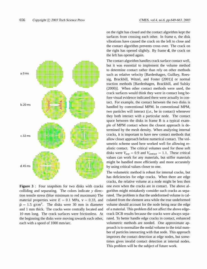
The DCB analysis was for an opening crack. The resultsin this section give a simulation when crack contact isimportant. The simulation is for two disks moving to-wards each other, contacting, and then bouncing apart.The disk on the left has a horizontal crack in the mid-dle of the disk. The length of the crack is equal to onethird the diameter of the disk. The disk on the right hasthe same size crack but oriented in the vertical direction.When the disks first make contact, the axial compressionof the disk on the left causes mode I loading of the crackand the crack opens [Shetty, Rosenfield, and Duckworth(1987)]. The transverse compression to the disk on theright causes the cracks faces to contact and the contactalgorithm keeps the surfaces from crossing. After the im-pact event, the two disks begin to vibrate and the cracksopen and close. The contact algorithm keeps the solutionproceeding correctly.

The plots in Fig. 3 show four snapshots of the solution.The cracks are indicated by a black line and the colorsfor the material points indicate tensile stress in they di-rection. Framea shows the initial conditions with closedcracks and zero stress; the disks have initial velocitiestowards each other. Frameb shows a moment soon af-ter contact. The diametrical compression has opened thecrack in the left disk and red zones show crack tip stressconcentrations in they-direction normal stress. The crack


a. 0 ms

b. 20 ms

c. 32 ms

d. 45 ms

Figure 3 : Four snapshots for two disks with crackscolliding and separating. The colors indicatey direc-tion tensile stress (blue minimum to red maximum) Thematerial properties wereE = 0.1 MPa, ν = 0.33, andρ = 1.5 g/cm3. The disks were 30 mm in diameterand 1 mm thick. The cracks were centrally located and10 mm long. The crack surfaces were frictionless. Atthe beginning the disks were moving towards each other,each with a speed of 1000 mm/sec.

on the right has closed and the contact algorithm kept thesurfaces from crossing each other. In framec, the diskvibrations have caused the crack on the left to close andthe contact algorithm prevents cross over. The crack onthe right has opened slightly. By framed, the crack onthe left has opened again.

The contact algorithm handles crack surface contact well,but it was essential to implement the volume methodto determine contact rather than rely on other methodssuch as relative velocity [Bardenhagen, Guilkey, Roes-sig, Brackbill, Witzel, and Foster (2001)] or normaltraction methods [Bardenhagen, Brackbill, and Sulsky(2000)]. When other contact methods were used, thecrack surfaces would think they were in contact long be-fore visual evidence indicated there were actually in con-tact. For example, the contact between the two disks ishandled by conventional MPM. In conventional MPM,two particles will interact (i.e., be in contact) wheneverthey both interact with a particular node. The contactspace between the disks in frame B is a typical exam-ple of MPM contact where the closest approach is de-termined by the mesh density. When analyzing internalcracks, it is important to have new contact methods thatallow closer approach before numerical contact. The vol-umetric scheme used here worked well for allowing re-alistic contact. The critical volumes used for these softdisks wereVsep= 0.9 andVcontact = 1.1. These criticalvalues can work for any materials, but stiffer materialsmight be handled more efficiently and more accuratelyby using critical values closer to one.

The volumetric method is robust for internal cracks, buthas deficiencies for edge cracks. When there are edgecracks, the relative volume at a node might be less thenone even when the cracks are in contact. The above al-gorithm might mistakenly consider such cracks as sepa-rated. The problem is that the undeformed volume is cal-culated from the element area while the true undeformedvolume should account for the node being near the edgeof a material. This problem did not affect the above edge-crack DCB results because the cracks were always sepa-rated. To better handle edge cracks in contact, enhancedvolumetric methods are needed. One approximate ap-proach is to normalize the nodal volume to the total num-ber of particles interacting with that node. This approachimproves the contact detection at edge nodes, but some-times gives invalid contact detection at internal nodes.This problem will be the subject of future work.


3.3 Comparison to Experiment

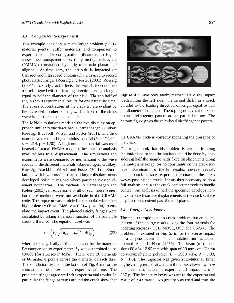
This example considers a much larger problem (58017material points), stiffer materials, and comparison toexperiments. The configuration, illustrated in Fig. 4shows five transparent disks (poly methylmethacylate(PMMA)) constrained by a jig to remain planar andaligned. At time zero, the left side is impacted (at6 m/sec) and high speed photography was used to recordphotoelastic fringes [Roessig and Foster (2001), Roessig(2001)]. To study crack effects, the central disk containeda crack aligned with the loading direction having a lengthequal to half the diameter of the disk. The top half ofFig. 4 shows experimental results for one particular time.The stress concentrations at the crack tip are evident bythe increased number of fringes. The front of the stresswave has just reached the last disk.

The MPM simulations modeled the five disks by an ap-proach similar to that described in Bardenhagen, Guilkey,Roessig, Brackbill, Witzel, and Foster (2001). The diskmaterial was set to a high modulus material (E = 174860,ν = .214,ρ = 1.90). A high modulus material was usedinstead of actual PMMA modulus because the analysisinvolved less total displacement. The simulations andexperiments were compared by normalizing to the wavespeeds in the different materials [Bardenhagen, Guilkey,Roessig, Brackbill, Witzel, and Foster (2001)]. Simu-lations with lower moduli that had larger displacementsdeveloped noise in regions where particles crossed el-ement boundaries. The methods in Bardenhagen andKober (2003) can solve some or all of such noise issues,but those methods were not available in the CRAMPcode. The impactor was modeled as a material with muchhigher density (E = 17486,ν = 0.214,ρ = 190) to em-ulate the impact event. The photoelasticity fringes werecalculated by taking a periodic function of the principlestress difference. The equation used was

cos

(kf

√(σxx−σyy

)2+4τ2xy

)(23)

wherekf is physically a fringe constant for the material.By comparison to experiments,kf was determined to be0.0889 (for stresses in MPa). There were 30 elementsor 60 material points across the diameter of each disk.The simulation results in the bottom of Fig. 4 are for thesimulation time closest to the experimental time. Thepredicted fringes agree well with experimental results. Inparticular the fringe patterns around the crack show that

Figure 4 : Five poly methylmethacylate disks impactloaded from the left side. the central disk has a crackparallel to the loading direction of length equal to halfthe diameter of the disk. The top figure gives the exper-iment birefringence pattern at one particular time. Thebottom figure gives the calculated birefringence pattern.

the CRAMP code is correctly modeling the presence ofthe crack.

One might think that this problem is symmetric alongthe mid-plane or that the analysis could be done by con-sidering half the sample with fixed displacements alongthe mid-plane except for no constraints on the crack sur-face. Examination of the full results, however, revealsthe the crack surfaces experience contact as the stresswaves pass by the crack. It was thus necessary to do afull analysis and use the crack contact methods to handlecontact. An analysis of half the specimen develops non-physical crack surface displacements as the crack surfacedisplacements extend past the mid-plane.

3.4 Energy Calculations

The final example is not a crack problem, but an exam-ination of the energy results using the four methods forupdating stresses - USL, MUSL, USF, and USAVG. Theproblem, illustrated in Fig. 5, is for transverse impacton a polymer specimen. The simulation mimics exper-imental results in Nairn (1989). The beam (of dimen-sions 88×6×12.95 mm with span of 68 mm) was Delrinpolyoxymethylene polymer (E = 2900 MPa,ν = 0.33,ρ = 1.5). The impactor was given a modulus 10 timeshigher, a higher density, and a thickness chosen to haveits’ total mass match the experimental impact mass of367 g. The impact velocity was set to the experimentalresult of 2.43 m/sec. No gravity was used and thus the


sum of kinetic and strain energy should remain constantthroughout the simulation.

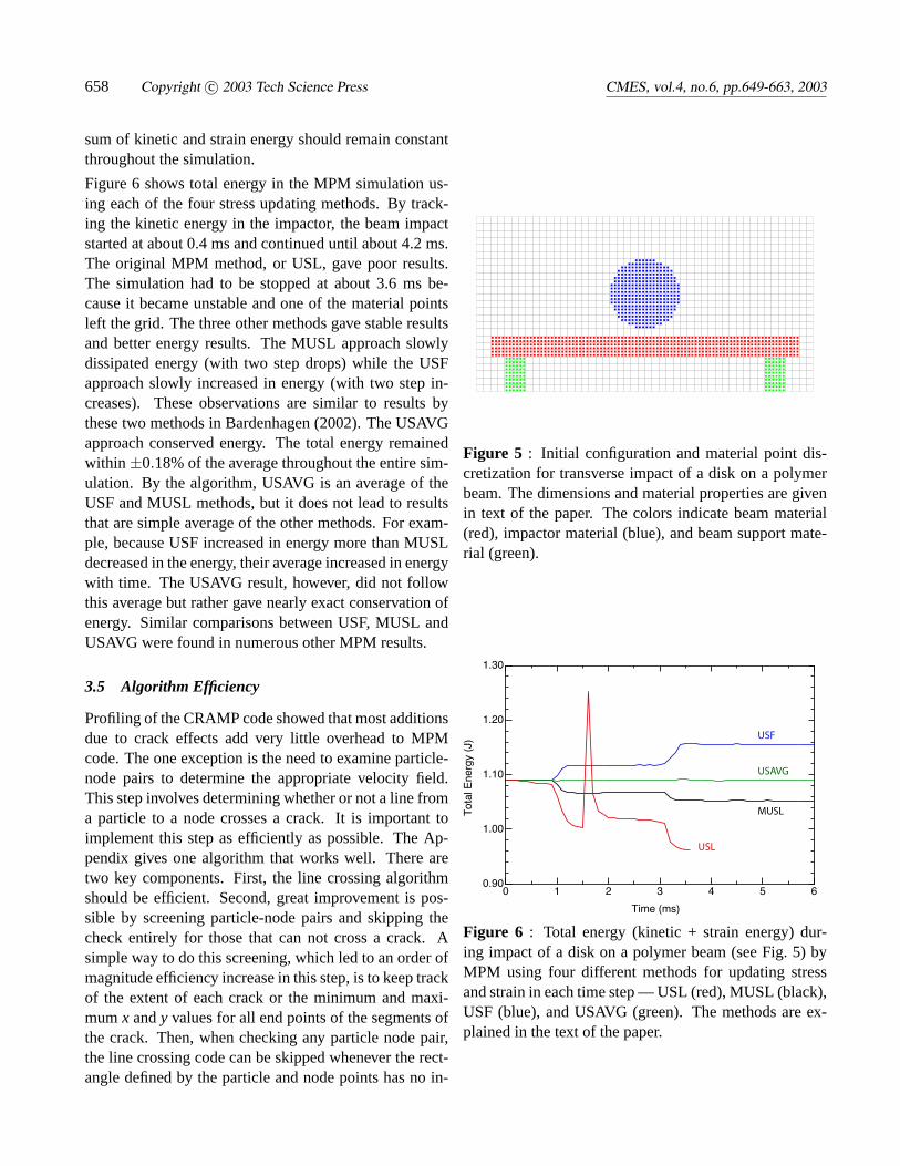
Figure 6 shows total energy in the MPM simulation us-ing each of the four stress updating methods. By track-ing the kinetic energy in the impactor, the beam impactstarted at about 0.4 ms and continued until about 4.2 ms.The original MPM method, or USL, gave poor results.The simulation had to be stopped at about 3.6 ms be-cause it became unstable and one of the material pointsleft the grid. The three other methods gave stable resultsand better energy results. The MUSL approach slowlydissipated energy (with two step drops) while the USFapproach slowly increased in energy (with two step in-creases). These observations are similar to results bythese two methods in Bardenhagen (2002). The USAVGapproach conserved energy. The total energy remainedwithin ±0.18% of the average throughout the entire sim-ulation. By the algorithm, USAVG is an average of theUSF and MUSL methods, but it does not lead to resultsthat are simple average of the other methods. For exam-ple, because USF increased in energy more than MUSLdecreased in the energy, their average increased in energywith time. The USAVG result, however, did not followthis average but rather gave nearly exact conservation ofenergy. Similar comparisons between USF, MUSL andUSAVG were found in numerous other MPM results.

3.5 Algorithm Efficiency

Profiling of the CRAMP code showed that most additionsdue to crack effects add very little overhead to MPMcode. The one exception is the need to examine particle-node pairs to determine the appropriate velocity field.This step involves determining whether or not a line froma particle to a node crosses a crack. It is important toimplement this step as efficiently as possible. The Ap-pendix gives one algorithm that works well. There aretwo key components. First, the line crossing algorithmshould be efficient. Second, great improvement is pos-sible by screening particle-node pairs and skipping thecheck entirely for those that can not cross a crack. Asimple way to do this screening, which led to an order ofmagnitude efficiency increase in this step, is to keep trackof the extent of each crack or the minimum and maxi-mumx andy values for all end points of the segments ofthe crack. Then, when checking any particle node pair,the line crossing code can be skipped whenever the rect-angle defined by the particle and node points has no in-

Figure 5 : Initial configuration and material point dis-cretization for transverse impact of a disk on a polymerbeam. The dimensions and material properties are givenin text of the paper. The colors indicate beam material(red), impactor material (blue), and beam support mate-rial (green).

0 1 2 3 4 5 60.90

1.00

1.10

1.20

1.30

Time (ms)

Tota

l Ene

rgy

(J) USF

USAVG

MUSL

USL

Figure 6 : Total energy (kinetic + strain energy) dur-ing impact of a disk on a polymer beam (see Fig. 5) byMPM using four different methods for updating stressand strain in each time step — USL (red), MUSL (black),USF (blue), and USAVG (green). The methods are ex-plained in the text of the paper.


tersection with the extent of the crack. With optimal line-crossing algorithm combined with screening using crackextents, the fracture calculations in this paper averagedonly 10% longer than the comparable MPM calculationwith no cracks.

4 Conclusions

This paper describes a CRAMP algorithm which extendsMPM to naturally handle explicit cracks. When the frac-ture code is written efficiently, especially the new linecrossing section, the CRAMP code achieves crack cal-culations with very letter extra cost in calculation time.The results show that CRAMP gets the correct MPM so-lutions and comparisons to both FEA and experimentsshow that it gets good results for crack problems. Toaccount for crack surface contact, there are checks forcontact and both stick and sliding with friction can behandled. The method to detect crack contact is robust forinternal cracks but may need some adjustment for prob-lems involving edge cracks. Crack propagation is eas-ily handled by simply moving the crack or adding cracksegments at any time step. The important problem thatremains is the calculation of crack tip or fracture param-eters followed by prediction of crack propagation. Thisproblem will be the subject of future work. Althoughthis paper describes a 2D algorithm, extension to 3D ispossible. In 3D, the crack line needs to be replaced bya crack surface described by planar elements instead linesegments. The line crossing algorithm needs to be re-placed by a 3D area crossing algorithm.

Acknowledgement: This work was support by a grantfrom the Department of Energy DE-FG03-02ER45914and by the University of Utah Center for the Simulationof Accidental Fires and Explosions (C-SAFE), funded bythe Department of Energy, Lawrence Livermore NationalLaboratory, under Subcontract B341493.

References

Atluri, S. N.; Shen, S. (2002): The Meshless Lo-cal Petrov-Galerkin (MLPG) method: A Simple & Less-Costly Alternative to the Finite Element and BoundaryElement Methods.Computer Modeling in Engineering& Sciences, vol. 3, pp. 11–52.

Atluri, S. N.; Shen, S. P.(2002): The Meshless LocalPetrov-Galerkin (MLPG) Method. Tech. Science Press.

Atluri, S. N.; Zhu, T. (1998): A New MeshlessLocal Petrov-Galerkin (MLPG) Approach in Computa-tional Mechanics. Computational Mechanics, vol. 22,pp. 117–127.

Bardenhagen, S. G.(2002): Energy Conservation Errorin the Material Point Method.J. Comp. Phys., vol. 180,pp. 383–403.

Bardenhagen, S. G.; Brackbill, J. U.; Sulsky, D.(2000): The Material Point Method for Granular Ma-terials. Computer Methods in Applied Mechanics andEngineering, vol. 187, pp. 529–541.

Bardenhagen, S. G.; Guilkey, J. E.; Roessig, K. M.;Brackbill, J. U.; Witzel, W. M.; Foster, J. C. (2001):An Improved Contact Algorithm for the Material PointMethod and Application to Stress Propagation in Gran-ular Material. Computer Modeling in Engineering &Sciences, vol. 2, pp. 509–522.

Bardenhagen, S. G.; Kober, E. M.(2003): The Gen-eralized Interpolation Material Point Method. in press,2003.

Batra, R. C.; Batra, H.-K. (2002): Analysis of Elas-todynamic Deformations Near a Crack/Notch Tip by theMeshless Local Petrov-Galerkin (MLPG) Method.Com-puter Modeling in Engineering & Sciences, vol. 3, pp.717–730.

Belytschko, T.; Lu, Y. Y.; Gu, L. (1994): Element-FreeGalerkin Methods. Int. J. Num. Meth. Engrg., vol. 37,pp. 229–256.

Belytschko, T.; Tabbara, M. (1996): Dynamic Frac-ture Using Element-Free Galerkin Methods.Int. J. Nu-mer. Methods in Eng., vol. 39, pp. 923–938.

Ching, H.-K.; Batra, R. C. (2001): Determinationof Crack Tip Fields in Linear Elastostatics by the Mesh-less Local Petrov-Galerkin (MLPG) Method.ComputerModeling in Engineering & Sciences, vol. 2, pp. 273–289.

Guilkey, J. E.; Weiss, J. A. (2002): Implicit TimeIntegration for the Material Point Method: Quantitativeand Algorithmic comparisons with the Finite ElementMethod. in press, 2002.


Nairn, J. A. (1989): The Measurement of PolymerViscoelastic Response During an Impact Experiment.Polym. Eng. & Sci., vol. 29, pp. 654–661.

Organ, D. J.; Fleming, M.; Belytschko, T. (1996):Continuous Meshless Approximations for NonconvexBodies by Diffraction and Transparency.ComputationalMechanics, vol. 18, pp. 225–235.

Parker, S. G. (2002): A Component-based Ar-chitecture for Parallel Multi-Physics PDE Simulation.In International Conference on Computational Science(ICCS2002) Workshop on PDE Software.

Roessig, K. M.(2001): 2001. Personal communication.

Roessig, K. M.; Foster, J. C.(2001): Experimen-tal Simulations of Dynamic Stress Bridging in PlasticBonded Explosives. in press, 2001.

Shetty, D. K.; Rosenfield, A. R.; Duckworth, W. H.(1987): Mixed-Mode Fracture in Biaxial Stress State:Application of the Diametral-Compression (BrazilianDisk) Test. Eng. Fract. Mech., vol. 26, pp. 825–839.

Sulsky, D.; Chen, Z.; Schreyer, H. L.(1994): A Par-ticle Method for History-Dependent Materials.Comput.Methods Appl. Mech. Engrg., vol. 118, pp. 179–186.

Sulsky, D.; Schreyer, H. K. (1996): AxisymnmetricForm of the Material Point Method with Applications toUpsetting and Taylor Impact Problems.Comput. Meth-ods. Appl. Mech. Engrg, vol. 139, pp. 409–429.

Sulsky, D.; Zhou, S.-J.; Schreyer, H. L.(1995): Appli-cation of a Particle-in-Cell Method to Solid Mechanics.Comput. Phys. Commun., vol. 87, pp. 236–252.

Tan, H.; Nairn, J. A. (2002): Hierarchical AdaptiveMaterial Point Method in Dynamic Energy Release RateCalculations. Comput. Meths. Appl. Mech. Engrg., vol.191, pp. 2095–2109.

Zhou, S.-J.(1998): The Numerical Prediction of Ma-terial Failure Based on the Material Point Method. PhDthesis, Department of Mechanical Engineering, Univer-sity of New Mexico, 1998.

Appendix A: CRAMP Algorithm

This appendix summarizes the CRAMP algorithm to in-clude explicit cracks and some revisions to MPM to up-date stresses and strains by a method that minimizes dis-sipation of energy. The algorithm is for 2D calculations,but most vector results translate easily into a 3D algo-rithm. In the following, subscriptp always refers toa particle property, subscripti always refers to a nodalproperty, bold face refers to a vector or a tensor, plaintext refers to a scalar, and an over bar indicates a spe-cific quantity (actual quantity divided by particle den-sity). The following single algorithm includes four op-tions for updating particle stresses and strains denoted asUSL, MUSL, USF, and USAVG; these methods were de-scribed in the text of the paper.

Task 0: At the beginning of the(k+1)th MPM analysisstep, all information for the numerical solution resideson the particles. The information relevant to the fol-low algorithm are particle position (xk

p), velocity (vkp),

specific stress (σkp), strain (εk

p), mass (mp), density (ρp),thickness (tp for 2D calculations), and any other mate-rial properties needed for constitutive law calculations.The shape functions and shape function gradients aredefined from the current particle positions as

Ski,p = Ni(xk

p) and Gki,p = ∇Ni(xk

p) (24)

whereNi(x) are the basic element shape functions. Inpractice, the shape functions and their gradients are notcalculated and stored (which would require a large ar-ray), but anytime they are calculated during the algo-rithm, they refer to the particle position at the beginningof the (k+ 1)th step. The particle volume, which is anarea in 2D calculations, is found from

Vkp = (1+ εk

p,xx)(1+ εkp,yy)

mp

ρptp(25)

Task 1: Loop over the particles. For each particle, drawa line from that particle to each node in the element con-taining that particle and use a line-crossing algorithm tocalculateν(p, i) = 0, 1, or 2 which determines the ve-locity field for particlep at nodei. An optimized line-crossing algorithm is given below. Field 0 means thedrawn line does not cross a crack; field 1 means the linecrosses a crack and the particle is above the crack rela-tive to the node; field 2 means the line crosses a crack


and the particle is below the crack relative to the node.If ν(p, i) = 1 or 2 and nodei does not have that ve-locity field, then allocate a new velocity field for thatnode. Only nodes near cracks will have multiple veloc-ity fields and except in unusual conditions, no node willever have more than two velocity fields — one for par-ticles on one side of the crack and one for particles onthe other side.

In the same loop, calculate nodal momenta and lumpedmasses for all needed velocity fields using

pki, j =

np

∑p=1

mpvkpSk

i,pδ j,ν(p,i) j = 0,1,2

mDki, j =

np

∑p=1

mpSki,pδ j,ν(p,i) j = 0,1,2

(26)

whereδi,ν(p,i) is the Kronecker delta function. For usein the contact algorithm, calculatetotal nodal volumesusing

Vki =

np

∑p=1

VkpSk

i,p (27)

Task 2: Apply any boundary conditions to nodal mo-menta calculated in the previous task and check forcrack contact by the procedure listed below. For USFor USAVG methods only, update particle stresses andstrains by the procedure listed below. The new particlestresses and strains are denotedσk′

p andεk′p . For USL

and MUSL methods, the stresses and strains are not up-dated and thus setσk′

p = σkp andεk′

p = εkp.

Task 3: Loop over the particles again. For each particlecalculate internal, external, and total forces for all ve-locity fields in use. The equations [Sulsky, Chen, andSchreyer (1994), Sulsky, Zhou, and Schreyer (1995)]now adjusted for multiple velocity fields are (each forj = 0, 1, 2):

f inti, j =

np

∑p=1

(−mpσk′

p ·Gki,p +mpbpSk

i,p

)δ j,ν(p,i)

f exti, j =

np

∑p=1

f kpSk

i,pδ j,ν(p,i)

f toti, j = f int

i, j + f exti, j −κpk

i, j

(28)

wherebp are any specific body forces on a particle, suchas gravity,f k

p are forces applied directly to particles, andκ is a damping constant which can be used to damp theanalysis. If any nodes have fixed displacement inx or

y directions, set the total forces for all velocity fields atthat node to zero to prevent acceleration in the next task.

Task 4: Update nodal point momenta

pk′i, j = pk

i, j +∆t f toti, j j = 0,1,2 (29)

Adjust any momenta for crack contact effects by theprocedure listed below.

Task 5: Loop over the particles to update particle po-sition and velocity using Sulsky, Zhou, and Schreyer(1995):

xk+1p = xk

p +∆tnn

∑i=1

pk′i,ν(p,i)S

ki,p

mDki,ν(p,i)

vk+1p = vk

p +∆tnn

∑i=1

f toti,ν(p,i)S

ki,p

mDki,ν(p,i)

(30)

Notice that the momentum, force, and mass used is thisupdate come from the specific velocity field for eachparticle/node pair determined by the line crossing re-sults forν(p, i) evaluated in Task 1.

Task 6: a. For USL method only, update particlestresses and strains as described below to findσk+1

p and

εk+1p and setpk′′

i, j = pk′i, j for later use.

b. For USF only, the stress and strain update was donebefore and thus setσk+1

p = σk′p , εk+1

p = εk′p . Also set

pk′′i, j = pk′

i, j for later use.

c. For MUSL or USAVG only, extrapolate the new par-ticle velocities to the grid to get a revised set of nodalmomenta using:

pk′′i, j =

np

∑p=1

mpvk+1p Sk

i,pδ j,ν(p,i) j = 0,1,2 (31)

Adjust any momenta for crack contact effects by theprocedure listed below. Note that this extrapolation usesthe new particle velocities but the shape functions andline crossing results from the original particle positions.This approach was found to give better results than oneusing updated information. Update particle stresses andstrains using the new nodal momenta by the procedurelisted below to findσk+1

p andεk+1p .

Task 7: Calculate center of mass velocity for each nodewith multiple velocity fields:

vki,cm =

∑3j=1pk′′

i, jϕi, j

∑3j=1mDk

i, j ϕi, j(32)


whereϕi, j = 1 if there exists ap such thatδ j,ν(p,i) = 1,otherwiseϕi, j = 0. In other words,ϕi, j is 1 or 0 depend-ing on whether or not velocity fieldj is present for nodei. Use this nodal velocity field to update the positionsof all line segments that define the cracks by standardposition updating methods.

Task 8: All information is now on the particles and ifneeded the cracks have translated. All nodal and meshinformation can be discarded and then return to Task 0to begin the next MPM calculation step.

Line Crossing Algorithm: The most time consuming,new calculation required for CRAMP is the line-crossing calculation in Task 2. It is important for thiscalculation to be optimal and precise. The only numer-ical difficulty occurs when a node lies very close to thecrack path. In some line-crossing algorithms, numericalround off in this situation could result in two particleson the same side of the crack being labeled as being onopposite sides. The complementary problem of whena material point lines very close to a crack path neveroccurs because the contact methods keep particles fromreaching the crack path.

A line-crossing algorithm in 2D based on signed ar-eas of certain triangles solved the problem of nodes oncracks. For any three points,x1, x2, andx3, the signedarea of the triangle with those vertexes is given by

Area= x1(y2−y3)+x2(y3−y1)+x3(y1−y2) (33)

This area is positive if the path fromx1 to x3 is counterclockwise, negative if it is clockwise, and zero if thepoints are collinear. Using this signed area, the algo-rithm is as follows:

Subtask 1: Before doing any calculations, determineif the rectangle defined by the particle (x1 = xp) andthe node (x2 = xn) under consideration intersects theextent of the segment endpoints in the crack. If it doesnot, the line does not cross the crack and rest of thealgorithm can be skipped for that crack.

Subtask 2: For each crack segment with endpointsx3

and x4, calculate the sign of the areas of triangles(123), (124), (341), and(342) denoted as “+”, “−”or “0”.

Subtask 3: The particle is above the crack if the signsare(−++−), (−++0), (0++0), or (−0+0). The

first case is the most common; the other three corre-spond to the node being on the crack segment, on thestart point of the crack segment, or on the end point ofthe crack segment, respectively. The cases where thematerial point is on the crack segment can be ignored.Similarly, the particle is below the crack if the signsare(+−−+), (+−−0), (0−−0), or (+0−0). Allother combinations of signs indicate the line does notcross the line segment. In practice, many signed areacalculations can be skipped. For example is the signsof (123) and(123) are(++), there is no need to eval-uate the signs of(341) and(342) because the line cannot cross the segment.

Subtask 4: One complication is that a givenxp to xn

line might cross more than one segment in a singlecrack. In this situation, the crossing is ignored unlessthere are an odd number of crossings. To include thispossibility, the previous two steps must check all seg-ments in a crack before deciding if there is a crossing,but if Subtask 1 finds no intersection, the check for allsegments in that crack can be skipped.

Contact Algorithm: Any time the nodal momenta arecalculated (i.e., in Tasks 2, 4, and 6c), the above al-gorithm must check cracks for contact. If contact isfound, adjust nodal momenta for all velocity fields atnodes experiencing contact. If any momenta changein Task 4, back calculate the corresponding total nodalforces to match the new momenta. This recalculation isneeded to insure particle velocities update correctly inTask 5. The algorithms for deciding on contact and foradjusting momenta are given in theMPM With ExplicitCrackssection.

Updating Stresses and Strains:Because the above al-gorithm includes four different methods for updatingstresses and strains (USL, MUSL, USF, and USAVG),it includes several locations for the updates (Tasks 2, 6a,and 6c). All stress and strain updates use the followingprocedure:

Subtask 1: Calculate nodal point velocities using thecurrent nodal point momenta

vi, j =pk∗

i, j

mDk∗i, j

j = 0, 1, 2 (as needed) (34)

wherek∗means the most recently calculated momentaand vi, j is only calculated for active velocity fields(ϕi, j = 1).


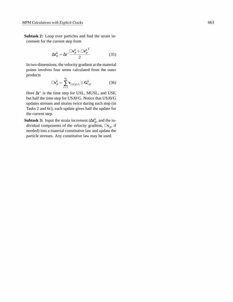
Subtask 2: Loop over particles and find the strain in-crement for the current step from

∆εkp = ∆t∗

∇vkp +∇vk

pT

2(35)

In two dimensions, the velocity gradient at the materialpoints involves four terms calculated from the outerproducts

∇vkp =

nn

∑i=1

vi,ν(p,i)⊗Gki,p (36)

Here∆t∗ is the time step for USL, MUSL, and USF,but half the time step for USAVG. Notice that USAVGupdates stresses and strains twice during each step (inTasks 2 and 6c); each update gives half the update forthe current step.

Subtask 3: Input the strain increment (∆εkp, and the in-

dividual components of the velocity gradient,∇vp, ifneeded) into a material constitutive law and update theparticle stresses. Any constitutive law may be used.

Documents

Material Point Method Calculations with Explicit Cracksguilkey/MPMPubs/NairnMPMCracks.pdf · Material Point Method Calculations with Explicit Cracks ... periments show it gets good