Embed Size (px)
Citation preview

October 26, 2019 12:21 Handbook on Big Data and. . . — Vol. 1 – 9.61in x 6.69in b3639-v1-ch03 3rd Reading page 65
Chapter 3
Materials Informatics and Data System forPolymer Nanocomposites Analysis and Design
Wei Chen∗,‖, Linda Schadler†, Cate Brinson‡, Yixing Wang∗, Yichi Zhang∗,Aditya Prasad¶, Xiaolin Li§ and Akshay Iyer∗
∗Department of Mechanical Engineering, Northwestern University,2145, Sheridan Rd., Evanston, IL 60208–3111, USA
†College of Engineering and Mathematical Sciences, University of Vermont,Burlington, VT 05405, USA
‡Department of Mechanical Engineering and Materials Science,Duke University, Durham, NC 27708, USA
§Theoretical & Applied Mechanics, Northwestern University,2145, Sheridan Rd., Evanston, IL 60208–3111, USA
¶Department of Materials Science and Engineering, Rensselaer PolytechnicInstitute, 110 8th St, Troy, NY 12180, USA
The application of Materials Informatics to polymer nanocompositeswould result in faster development and commercial implementation ofthese promising materials, particularly in applications requiring a uniquecombination of properties. This chapter focuses on a new data resourcefor nanocomposites — NanoMine — and the tools, models, and algorithmsthat support data-driven materials design. The chapter begins with a briefintroduction to NanoMine, including the data structure and tools available.Critical to the ability to design nanocomposites, however, is developingrobust structure–property–processing (s–p–p) relationships. Central to thisdevelopment is the choice of appropriate microstructure characterizationand reconstruction (MCR) techniques that capture a complex morphologyand ultimately build statistically equivalent reconstructed composites foraccurate modeling of properties. A wide range of MCR techniques isreviewed followed by an introduction of feature selection and feature extrac-tion techniques to identify the most significant microstructure features
65
October 26, 2019 12:21 Handbook on Big Data and. . . — Vol. 1 – 9.61in x 6.69in b3639-v1-ch03 3rd Reading page 66
66 W. Chen et al.
for dimension reduction. This is then followed by examples of using adescriptor-based representation to create processing–structure (p–s) andstructure–property (s–p) relationships for use in design. To overcome thedifficulty in modeling the interphase region surrounding nanofillers, anadaptive sampling approach is presented to inversely determine the inter-phase properties based on both FEM simulations and physical experimentdata of bulk properties. Finally, a case study for nanodielectrics in acapacitor is introduced to demonstrate the integration of the p–s and s–prelationships to develop optimized materials for achieving multiple desiredproperties.
1. Introduction
The past 5 years have seen substantial growth in access to digital materialsdata with the goal to accelerate materials design under the national Mate-rials Genome Initiative (MGI).1–4 New materials informatics techniques4–10
are being developed to centralize materials data and include informationacross a significant range of length and time scales in order to improveuse of data mining, statistics, image processing and visualization, andpredictive analytics over the lifecycle development of materials systems.However, unlike the metallic and inorganic alloy fields, polymers and theirnanocomposites are less developed in both database system and data-driven analytical protocols. The complexity and high dimensionality ofthe polymer and polymer nanocomposite data space, including details onprocessing conditions, nanoscale filler dispersion, as well as properties, makeit challenging to implement a universal standard that could archive allpossible nanocomposite data and facilitate the intentional design of polymernanocomposites. Additionally, small changes in processing conditions orsurface chemistry can result in drastic changes in filler–matrix interactionand filler microstructure, which can cause significant changes in compositeproperties.11 These factors all hinder the establishment of a comprehensivemethodology to fully incorporate processing, structure, and property (p–s–p) information for nanocomposite materials into the design process. Instead,the design and development of new nanocomposite materials remains largelydependent on Edisonian, trial-and-error iterations. To improve our abilityto design nanocomposites, it is essential to gain a deeper mechanisticunderstanding of, and the ability to map and quickly search, the p–s–p spacefor new polymer nanocomposite systems.
To meet these challenges, this chapter presents a data-centric approach toaccelerate the development of next-generation nanostructured polymers withunprecedented and predictable combinations of properties. The proposed

October 26, 2019 12:21 Handbook on Big Data and. . . — Vol. 1 – 9.61in x 6.69in b3639-v1-ch03 3rd Reading page 67
Materials Informatics and Data System 67
approach integrates physics-based models, empirical data, machine learningapproaches, and a robust interphase model built using curated and custom-generated data, within a novel microstructural analysis and optimal designframework. The implementation of this approach is further enhanced bycreating an open nanocomposite data resource (“NanoMine”a), an integralpart of the national effort under the MGI and the Integrated ComputationalMaterials Engineering (ICME) initiative.12 However, a data resource itselfis not sufficient for innovative material design. The data resource mustbe coupled with newly developed tools, models, and algorithms for data-driven material design. Critically, new models for interphase properties, bothphysics-based and from machine learning, are needed to create meaningfulp–s–p work flows.
In this chapter, we present the architecture of the NanoMine data systemand the backbone behind it, an integrated framework for microstructuralanalysis, and optimal material design. Microstructure analysis plays a keyrole in assessing p–s–p relationships and in the design of micro- andnanostructured materials systems like polymer nanocomposites. Centralto microstructural analysis is the method of MCR, which consists ofstatistical methods to quantitatively represent the microstructure and itspossible inherent randomness (aka characterization) and build ensembles ofstatistically equivalent microstructures13 (aka reconstruction). MCR allowsone to systematically go beyond the limits where empirical data areavailable and build forward and inverse p–s–p links through simulation-basedanalysis and design. While the nanocomposite materials design problemcan be formulated as an optimization problem through parametric-basedmicrostructure representation, two challenging research questions remain: (1)how to quantitatively represent a heterogeneous microstructure system usinga small set of physically meaningful variables (“microstructure representa-tion”), and (2) how to effectively explore the vast, high-dimensional designspace to search for optimal material designs that can be readily synthesizedthrough processing (“design synthesis”).
As shown in Figure 1, our proposed microstructural analysis and optimalmaterials design framework is a multi-phase process in which image analysisis first utilized to analyze physical samples made from existing processes.After a digital representation of filler and matrix materials is obtained
aNanoMine can be accessed at http://nanomine.org. The site is still under development;the tools will be continuously updated and new capabilities will be added.

October 26, 2019 12:21 Handbook on Big Data and. . . — Vol. 1 – 9.61in x 6.69in b3639-v1-ch03 3rd Reading page 68
68 W. Chen et al.
Image Preprocessing
• Filtering• Threshold• Local Threshold
Microstructure Characteriza on &
Reconstruc on (MCR)
• Correla on func on• Descriptor-based• Spectral density func on• machine learning
Dimension Reduc on & Machine Learning for
p-s-p modeling op miza onMaterial Design
• Metamodeling• Mul criteria op miza on
• Feature selec on (PCA)• Feature extrac on
(Structural Equa on Modeling)
• Physics-aware: Spectral density func on
Figure 1: Microstructural analysis and optimal materials design framework.
through “Image Preprocessing”, a range of techniques can be consideredfor MCR. We have developed and implemented a suite of MCR techniquesin NanoMine, such as correlation functions,14 descriptor-based methods,15,16
and spectral density functions (SDFs). As indicated by details provided inSection 3, there are pros and cons associated with each technique; some of thetechniques are either too high-dimensional, prohibitive for 3D digital recon-struction, or not applicable to arbitrary shaped nanofillers and local aggre-gation. For physically meaningful p–s–p mappings and quick exploration ofmicrostructure designs that include processing feasibility, there is a need for“Dimension Reduction and Machine Learning” to identify the reduced-orderrepresentation of microstructures. In this chapter, we will present the useof machine learning17 and structure equation modeling (SEM) techniques18
to determine the key microstructure descriptors and processing descriptorsin studying the processing–structure and structure–property relationships.In addition, physics-aware dimension-reduction methods, such as the SDF-based approach, are presented as powerful techniques for representing generalmaterial systems with high dimensionality and complex, irregular shapes ofmicrostructures. In the last stage of “Material Design Optimization”, eitherthe descriptor-based or SDF-based microstructure representation enablesefficient reconstructions and allows the use of a parametric optimizationapproach to search for the optimal microstructure design.16 In this stage,high-throughput simulation data is used to construct surrogate metamodelsfor rapid design evaluations, and multi-criteria optimization is utilizedto generate a set of materials design solutions for achieving multipleproperties.
In the remaining part of this chapter, we first describe the majorcomponents of the NanoMine data system and a robust ontology for polymernanocomposites supporting organization, search, and visualization servicesof the material data (Section 2). This is followed by an introduction ofmultiple MCR techniques (Section 3). Dimension reduction techniques formanaging the complexity of microstructure representation are presented inSection 4. In Section 5, we provide details of using data mining techniques

October 26, 2019 12:21 Handbook on Big Data and. . . — Vol. 1 – 9.61in x 6.69in b3639-v1-ch03 3rd Reading page 69
Materials Informatics and Data System 69
for constructing descriptor-based p–s relationships based on experimentaldata. Finite-element-based s–p prediction is presented in Section 6 wherea combined physics-based and data-assisted modeling approach is utilized.While the overall model is physics-based, an adaptive optimization approachis used to calibrate the interphase model based on the collected physicaldata. Finally, in Section 7, a capacitor design problem is used as an exampleto demonstrate the full integration of p–s and s–p models presented inearlier sections for design of nanodielectric materials using multi-criteriaoptimization. A model system not typically used for capacitors, but forwhich we have significant data, polymethylmethacrylate (PMMA)-basednanocomposite with silica nanoparticles, surface modified with a monofunc-tional chlorosilane, is used as the candidate material system for the casestudy.
2. NanoMine Data System and Data Resources
During past decades, extensive research efforts have focused on propertyenhancement of nano-reinforced polymeric materials using both simulationand experimental methods.19–21 Results from these studies have generated atremendous amount of data in different forms such as images, plots, andtext for a wide range of polymer, particle, and chemistry combinations.However, most of the research data reported in the literature lack a unifieddata format, terminology and uncertainty measures, and are incomplete.Conventional keyword-based web search engines cannot provide sufficientlydetailed and annotated search results for effective material design or evensimple exploratory query and comparison of facts. Consequently, it is hardto perform a comprehensive access or search of data according to user-specified criteria, making the design of new functional materials extremelyinefficient.
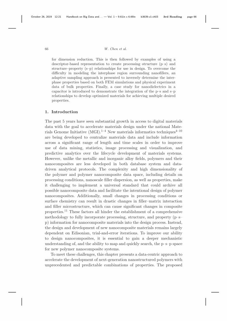
Using the Material Data Curator System (MDCS) developed at theNational Institute of Standards and Technology (NIST) and with sponsor-ship from the National Science Foundation, we have developed a prototypesystem for nanocomposite material data curation, exploration, and analysis,termed “NanoMine” (www.nanomine.org). NanoMine currently consists of agrowing nanocomposite database, a collection of module tools for statisticallearning, MCR, and simulation software to model bulk nanopolymer compos-ite material response (see Figure 2). The underlying principle of NanoMineis to create a living, open-source data resource for nanocomposites thatprovides data archiving and exchange, statistical analysis, and physics-basedmodeling for property prediction and materials design.
October 26, 2019 12:21 Handbook on Big Data and. . . — Vol. 1 – 9.61in x 6.69in b3639-v1-ch03 3rd Reading page 70
70 W. Chen et al.
Figure 2: Major features of NanoMine and the key features in each component.
The current NanoMine database contains more than 1,200 sampleswith extensive information on p–s–p domains manually curated from over150 papers as well as unpublished lab-generated data. It contains threesimulation tools for studying the electrical and mechanical response ofcomposite materials that include explicit representation of the interphase.Additionally, it has four statistical learning and analysis modules includingdownloadable packages that can be used to pre-process and analyze structureand property data. Continuous efforts have been made to expand the volumeof the database and include state-of-the-art microstructure analysis anddesign tools for the community.
2.1. NanoMine database and data schema
The NIST MDCS is an open-source platform providing solutions to collect,share, and transfer material data. The system provides basic functions fordata curation (data entry using a web-based system) and data exploration(search data by user specified criterion). MDCS is inherently a No-SQLdatabase that organizes the data using a user-defined data structure orschema.
A well-defined data structure, or schema, is crucial to effectively collectand archive materials data, enable efficient data retrieval, and facilitatedata exchange.22 In order to provide a standard schema to archive thenanocomposite data, the terminology in the schema should be unified andthe data types for storing the entities should be well-defined and self-explanatory.23 In order to develop the customized template to archive

October 26, 2019 12:21 Handbook on Big Data and. . . — Vol. 1 – 9.61in x 6.69in b3639-v1-ch03 3rd Reading page 71
Materials Informatics and Data System 71
Table 1: Summary of parameters in NanoMine data schema.
Section Description Examples
Data source Metadata of the source ofliterature.
DOI, author list, journalpublication year.
Materials Characteristics of constituentmaterials, polymer, particle,and functional groups.
Chemical structure, MW,density, volume fraction,surface treatment, graftdensity.
Processing Extraction from Experimentsection. Step-by-stepdescription of synthesis/characterization conditions.
Solution processing, meltmixing, polymerization.
Characterization Measurement equipment andparameters.
SEM/TEM, DMA, DSC, FTIR.
Properties Function data, value, andobservation of properties.
Modulus, dielectric constant,conductivity.
Microstructure Nanophase dispersion capture ingrayscale images. Quantifiedin morphological descriptors.
MAT file containing grayscaleimage matrix, descriptors(e.g., filler nearest centerdistance, equivalent radius).
the raw p–s–p parameters from data sources, 30 representative papers onpolymer nanocomposites published within the past decade were investigatedto find the most commonly recurring parameters and terminologies. Based onthe literature survey, a prototype data template was developed and servedas an initial structure to manage all the key parameters associated withp–s–p along with the metadata. The NanoMine data schema is continuouslyupdated to incorporate a wider range of parameters such as additionalprocessing methods or new properties.
As summarized in Table 1, the current NanoMine schema contains thefollowing six major sections:
(1) Data resource: The metadata of the source of the literature guided byDublin core standards which includes the DOI of the cited source, theauthors, title, keyword, time, and source of the publication.
(2) Materials: Material constituent information, including the filler parti-cle, polymer matrix, and surface treatments. The characteristics of purematrix and filler such as the polymer chemical structure and molecularweight and the particle density can be entered along with compositions(volume/weight fraction).
October 26, 2019 12:21 Handbook on Big Data and. . . — Vol. 1 – 9.61in x 6.69in b3639-v1-ch03 3rd Reading page 72
72 W. Chen et al.
(3) Processing: Sequential description of chemical syntheses and exper-imental procedures. The current template provides three major cate-gories: solution processing, melt mixing, and in situ polymerization. Foreach processing step, detailed information such as temperature, pressure,and time can be entered.
(4) Characterization: Information on material characterization equip-ment, methods, and condition used. This information includes detailson common microscopic imaging (SEM, TEM), thermal mechanical andelectrical measurement, as well as nanoscale spectroscopy.
(5) Properties: Measured data of material properties. Properties includemechanical, electrical, thermal, and volumetric properties. The propertydata could be in the format of a scalar, or in higher dimension such asin 2D spectroscopy or 3D maps.
(6) Microstructure: Raw microscopic grayscale images capturing thenanophase dispersion state. Geometric descriptors can also be includedto describe the statistical characteristics of the microstructure.
The three major data types used to store each entity are shown in Figure 3.Using the schema, the non-relational data structure is well-defined and
the raw XML document containing the nanocomposite data can be filled inreadily, with multiple data formats and dimensionality. The current curationprocess focuses on nanocomposites with surface-treated spherical inorganicfillers, where many analysis and simulation tools have already been developedinternally and the publications contained microscopic images with explicitdispersion information, well-documented processing and characterizationmethods, as well as clearly plotted property data.
Based on the NanoMine data schema, a robust ontology for polymernanocomposites has been developed to support organization, search, andvisualization services of the material data.24 This ontology also formalizesrelationships inherent in our XML schema and can act as a translator toaccept multiple XML formats, enhancing the ability to share across differentdata resources. On top of the NanoMine ontology, we are building a searchand visualization dashboard to allow users to browse and look up the databy using a simple query as shown in Figure 4.
2.2. Analysis tools in NanoMine
Apart from the database, NanoMine also provides functionalities for quan-titative investigation of the curated data to assist in property predictionand material design. NanoMine aims to provide a practical suite of toolkits
October 26, 2019 12:21 Handbook on Big Data and. . . — Vol. 1 – 9.61in x 6.69in b3639-v1-ch03 3rd Reading page 73
Materials Informatics and Data System 73
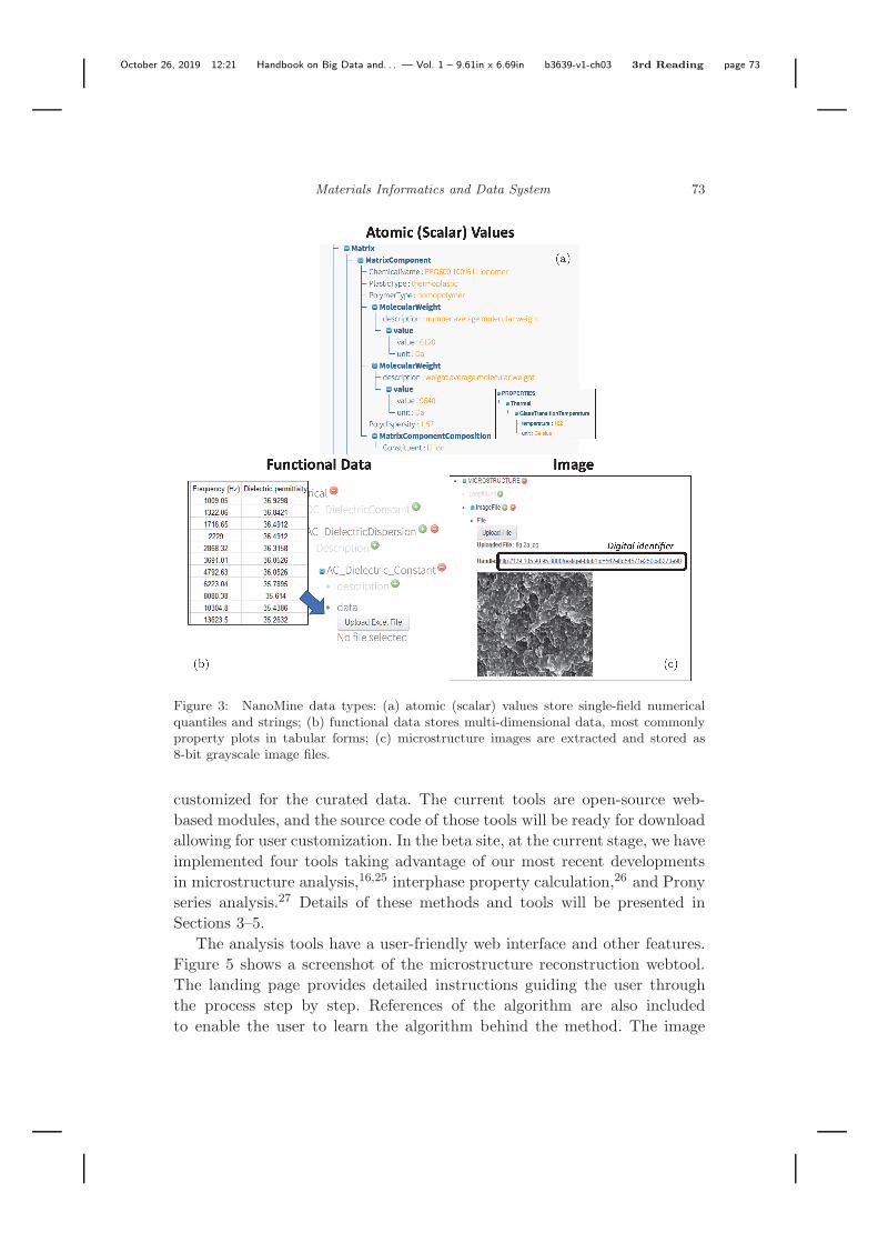
Figure 3: NanoMine data types: (a) atomic (scalar) values store single-field numericalquantiles and strings; (b) functional data stores multi-dimensional data, most commonlyproperty plots in tabular forms; (c) microstructure images are extracted and stored as8-bit grayscale image files.
customized for the curated data. The current tools are open-source web-based modules, and the source code of those tools will be ready for downloadallowing for user customization. In the beta site, at the current stage, we haveimplemented four tools taking advantage of our most recent developmentsin microstructure analysis,16,25 interphase property calculation,26 and Pronyseries analysis.27 Details of these methods and tools will be presented inSections 3–5.
The analysis tools have a user-friendly web interface and other features.Figure 5 shows a screenshot of the microstructure reconstruction webtool.The landing page provides detailed instructions guiding the user throughthe process step by step. References of the algorithm are also includedto enable the user to learn the algorithm behind the method. The image

October 26, 2019 12:21 Handbook on Big Data and. . . — Vol. 1 – 9.61in x 6.69in b3639-v1-ch03 3rd Reading page 74
74 W. Chen et al.
Figure 4: Examples of searching and visualization of NanoMine data shown in a list (onlyone entry shown for clarity and space constraints) (a) or a plot (b).
input format, correlation function for characterization/reconstruction, andnumber of reconstructed images can be chosen by the user. All computationsare performed on the NanoMine web server, and an email is sent to theuser after their request has been completed. Each user request is associatedwith a unique “Job ID” which ensures data privacy and can be used toretrieve, and download, a result at any time. Figure 5 shows a screenshotfrom NanoMine depicting the results of a reconstruction request using thetwo-point autocorrelation tool.
2.3. Simulations tools in NanoMine
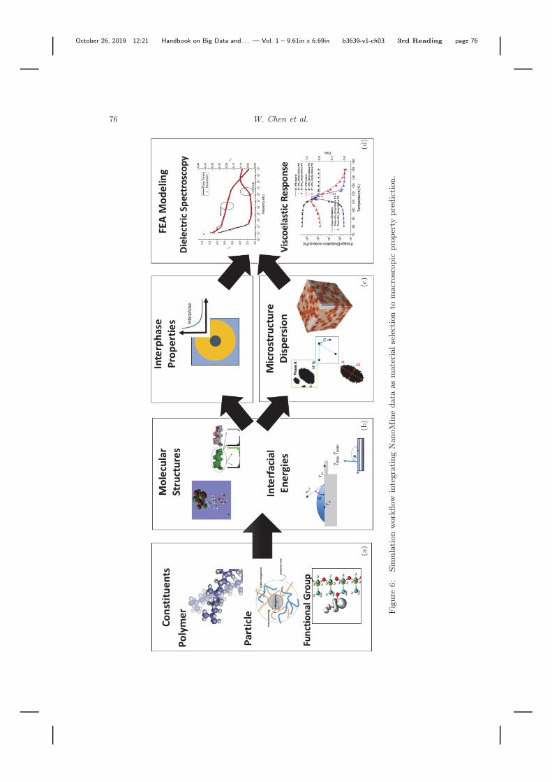
NanoMine also includes a set of physics-based continuum models and simu-lation tools for predicting the macroscopic material response. FEA modelshave been developed to predict the electrical and viscoelastic responseof the nanocomposite with explicit input of microstructure and detailedrepresentations of the interphase. The system currently has implementedtwo FEA models as web-tools to simulate the viscoelastic28 and dielectricalproperties.29,30 The available data in the database can be used as inputto the FEA model, which then predicts the composite properties. Figure 6shows the workflow of the simulations tools integrating with the curated dataand analysis tools introduced before. The material constituents, includingmolecular structure, can be obtained from the curated data. The material

October 26, 2019 12:21 Handbook on Big Data and. . . — Vol. 1 – 9.61in x 6.69in b3639-v1-ch03 3rd Reading page 75
Materials Informatics and Data System 75
Figure 5: Screenshot from the NanoMine platform depicting the results of a reconstruc-tion result from source images.
molecular structures are used to derive the energetic terms that representthe surface energy and filler–matrix interaction.31 Those mixing energyparameters are then applied to predict the interphase properties and therepresentative microstructure30 if micrographs are not available. Taking theinput of interphase properties and microstructure dispersion, a 3D FEAmodel is built with commercial software (COMSOL/Abaqus) using an APIand subroutine to calculate the composite dielectric spectra or viscoelasticresponse. The simulation typically takes 30 minutes for a representativenanodielectric system of 50 clusters in a representative volume element(RVE). Similar to the analysis tools, users are assigned unique Job IDs uponsubmission of a task. The Job ID can be used to check the status of the joband retrieve the results.
2.4. Materials design in NanoMine
The workflow of material design using NanoMine is outlined in Figure 7.Using the platform, the user is able to conduct both property simulation(from left to right) given specific material constituents and processingcombinations, as well as material design (from right to left) in order to obtaindesired nanocomposite properties. Suppose the user would like to predict
October 26, 2019 12:21 Handbook on Big Data and. . . — Vol. 1 – 9.61in x 6.69in b3639-v1-ch03 3rd Reading page 76
76 W. Chen et al.
Fig
ure
6:
Sim
ula
tion
work
flow
inte
gra
ting
NanoM
ine
data
as
mate
rialse
lect
ion
tom
acr
osc
opic
pro
per
typre
dic
tion.

October 26, 2019 12:21 Handbook on Big Data and. . . — Vol. 1 – 9.61in x 6.69in b3639-v1-ch03 3rd Reading page 77
Materials Informatics and Data System 77
Figure 7: Application of NanoMine on property prediction and material design. Left toright: material property prediction from material selection to bulk composite properties.Right to left: design process starting from target properties to necessary materialcharacteristics.
dielectric permittivity for a PMMA-based nanosilica filled nanocomposite.The first step is to query the database for existing property data for PMMAand nanosilica as material input to the FEA and to calculate the relevantsurface energies using the embedded heuristic approach. Then analysis mod-ules are applied to reconstruct the microstructure and predict the interphaseproperties using statistical correlations among surface energies, processingparameters, structural descriptors, and interphase property descriptors. TheFEA model is then carried out to compute the dielectric spectra for thisspecific sample. This whole process is reversible: the user wants to finda specific material combination and processing steps that could lead toa desired property. If such data have already appeared in the literatureand been curated into the database, the solution is simple: just querythe database for such a sample and find the material constituents andassociated processing steps. However, in most the cases, the target propertyis not in the database and a user usually wishes to have multiple targets(such as high dielectric permittivity and elastic modulus). NanoMine isbeing further developed to tackle precisely this challenge. Starting from theexisting data, the analysis and simulation modules are coupled with a designoptimization algorithm and metamodeling to explore different combinationsof constituents, microstructure, and interphase descriptors to attain thisgoal. A comprehensive predictive framework will be built on top of theentire set of p–s–p data applying a combination of data mining models,

October 26, 2019 12:21 Handbook on Big Data and. . . — Vol. 1 – 9.61in x 6.69in b3639-v1-ch03 3rd Reading page 78
78 W. Chen et al.
optimization methods, and numerical simulations. Details of these techniquesare provided in the upcoming sections.
3. Microstructure Characterization and Reconstruction forPolymer Nanocomposites
This section provides details of the MCR techniques for polymer nanocom-posites. As a material’s morphology significantly influences its proper-ties,32,33 an essential task in the creation of process–structure–property(p–s–p) linkages is analyzing the morphology of microstructure(s). Theanalysis is quantitative, and its outcome is a deep understanding of howprocessing conditions influence the formation of microstructure and howthe microstructure in turn affects the properties. Material morphology canbe recorded (in 2 or 3 dimensions) through several imaging techniques —scanning electron microscopy (SEM), transmission electron microscopy(TEM), atomic force microscopy (AFM), computer tomography (CT), etc.,each providing morphological information in a distinct perspective andchosen based on the type of information one seeks. In their raw form, theseimages are stored as an array of pixel intensity values, often containing noise(random variation of brightness/color), and are not of much use. To analyzethe image and extract useful morphological features, the following three-stepstrategy is recommended:
(i) Image binarization: Binarization is the process of converting agrayscale image to a black and white image (assuming there are onlytwo phases — filler and matrix) by removing noise and consequentlysimplifying the analysis. It is accomplished by determining a thresholdfor pixel intensity of filler and matrix components. As its name suggests,binarized images are essentially an array composed of 0’s (displayedin black) and 1’s (white). Binarization algorithms are classified asglobal (single intensity threshold used for entire image) and adaptivethresholding (intensity thresholds varies in different regions of theimage). The most widely used image binarization methods are Otsu’smethod34 (global) and the Niblack algorithm35 (adaptive).
(ii) Microstructure characterization: Several methods have been devel-oped that can convert multi-dimensional microstructure morphologyrecorded in images into a set of functions (aka features/descriptors/predictors) that encode significant morphological details, i.e., charac-terize the microstructure. As in the case of imaging techniques, userscan choose the characterization method according to the application.

October 26, 2019 12:21 Handbook on Big Data and. . . — Vol. 1 – 9.61in x 6.69in b3639-v1-ch03 3rd Reading page 79
Materials Informatics and Data System 79
A common observation in all characterization methods is their statisti-cal nature, since most material systems are inherently associated withrandomness.
(iii) Microstructure reconstruction: After characterization, one canreconstruct a statistically equivalent microstructure(s)13 which embod-ies a prescribed set of features (obtained by image characterization orprovided by user) and can be used as a RVE for simulating materialbehavior via finite element analysis (which creates the structure–property linkage) or serve as a training dataset for machine learningalgorithms.36,37 Reconstruction is often reduced to an optimizationprocess solved by heuristic methods (due to nonlinearity and highdimensionality), leading to an ensemble of statistically equivalentreconstructions.
The choice of characterization method determines the type of reconstructionmethod applicable, i.e., the reconstruction algorithm must be consistentwith the characterization method and vice-versa. It must be noted thatalthough all characterization and reconstruction methods are applicable toany microstructure in general, certain methods are more suited to a materialsystem as compared to others. Hence, users must consider properties of inter-est, their corresponding length scales, and the availability of computationalresources to select an appropriate characterization/reconstruction method.The rest of this section provides an overview of three MCR techniquescurrently included in NanoMine: correlation functions, spectral densityfunctions, and physical descriptor-based approaches. A brief introductionof emerging machine learning-based MCR techniques is provided at the endof this section. A detailed discussion of these methods and other associatedtechniques is available in the review article by Bostanabad et al.38
3.1. Correlation functions for MCR
Correlation functions (especially spatial correlation functions), some of themost widely used MCR methods, contain valuable information about therelative positioning of phases in an image. They do so by operating onbinarized microstructure images and evaluating the probability distributionof a group of randomly chosen pixels obeying certain “rules”. Althoughcorrelation functions can be defined for a group of n pixels (aka n-pointcorrelation function), it has been noticed that two-point (pixel) correlationfunctions embody significant details39–41 and will be used in the followingdiscussion for sake of simplicity. Mathematically, a two-point correlation
October 26, 2019 12:21 Handbook on Big Data and. . . — Vol. 1 – 9.61in x 6.69in b3639-v1-ch03 3rd Reading page 80
80 W. Chen et al.
function ϕi2 for phase i can be expressed as
ϕi2(r1, r2) = 〈Mr1Mr2〉, (1)
where 〈·〉 denotes the expectation operator and r1 and r2 represent locationvector of points and M is a microstructure indicator functions such that:
M ={
1 if r1 ∈ phase i
0 otherwise.(2)
For an isotropic and stationary microstructure, ϕi2 will only depend on the
distance r between the two points (making computation efficient42,43). As aresult
ϕi2(r1, r2) = ϕi
2(|Δr12|) = ϕi2(r). (3)
Based on the type of “rule” imposed on the two points, the following threetwo-point correlation functions are defined (refer Figure 8):
(i) Autocorrelation function (Si2(r))39,40: The probability that two
randomly chosen points are occupied by phase i and is a measureof dispersion. Since many experimental characterization techniquesprovide structural information in the form of Si
2(r), it is one of themost widely used correlation functions.
(ii) Lineal path correlation (Li2(r))44: The probability of finding a line
segment connecting two randomly chosen points entirely in phase i.Li
2(r) is a measure of cluster geometry and connectivity of phase i butunderestimates these features due to the constraint of measuring alongstraight lines.
(iii) Cluster correlation (Ci2(r))32,45,46: The probability that two ran-
domly chosen points, occupied by phase i, are contained in the samecluster. This correlation contains important information about topolog-ical connectivity and is a superior structural signature as compared toSi
2(r) and Li2(r).
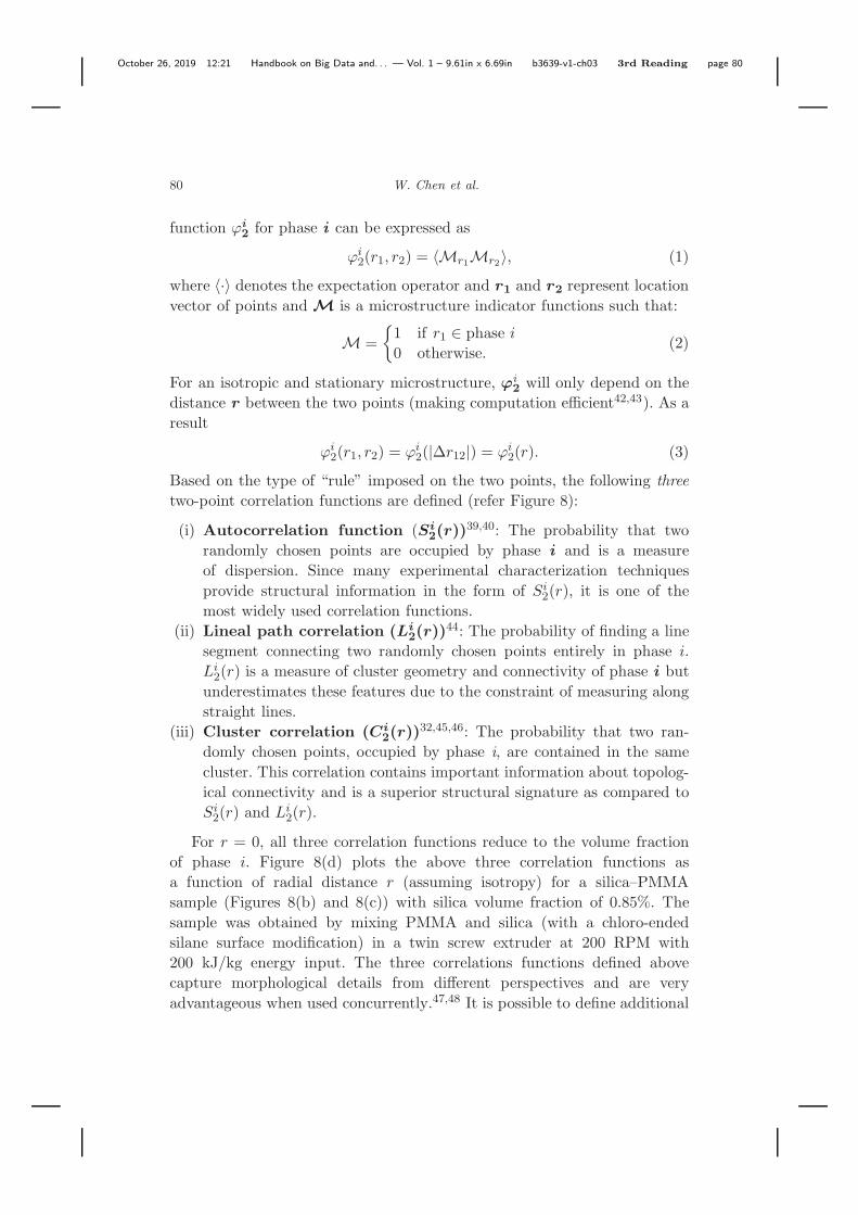
For r = 0, all three correlation functions reduce to the volume fractionof phase i. Figure 8(d) plots the above three correlation functions asa function of radial distance r (assuming isotropy) for a silica–PMMAsample (Figures 8(b) and 8(c)) with silica volume fraction of 0.85%. Thesample was obtained by mixing PMMA and silica (with a chloro-endedsilane surface modification) in a twin screw extruder at 200 RPM with200 kJ/kg energy input. The three correlations functions defined abovecapture morphological details from different perspectives and are veryadvantageous when used concurrently.47,48 It is possible to define additional

October 26, 2019 12:21 Handbook on Big Data and. . . — Vol. 1 – 9.61in x 6.69in b3639-v1-ch03 3rd Reading page 81
Materials Informatics and Data System 81
Figure 8: MCR using correlation functions: (a) a schematic representation of two-pointcorrelation functions for white phase; (b) a TEM image of silica-PMMA sample (silicavolume fraction ∼0.008, 1 pixel = 3.246 nm); (c) image (b) binarized using Niblackalgorithm — silica nanoparticles are white and PMMA is black; (d) plot of auto, linealpath, and cluster correlation function for silica; (e) and (f) two reconstructions of image(b) using Yeong–Torquato algorithm performed in NanoMine.
two-point correlation functions as well as higher-order functions such asthree-point and four-point correlation functions;32 however, they requiresignificantly more computational resource.
After characterization, reconstruction of statistically equivalent micro-structures can be cast as an optimization problem and tackled in thefollowing way:
(i) Start with a trial microstructure image which has the same volumefraction as the original image. A convenient initial microstructure usedwidely is a randomly generated white noise image.
(ii) Define an energy (cost) function which measures the difference betweenthe chosen correlation function(s) of the original and trial image.Mathematically, the energy function can be expressed as
I =n∑
i=1
m∑r=0
αi[ϕ0,i(r) − ϕt,i(r)]2, (4)

October 26, 2019 12:21 Handbook on Big Data and. . . — Vol. 1 – 9.61in x 6.69in b3639-v1-ch03 3rd Reading page 82
82 W. Chen et al.
where n is total number of correlation functions considered, m is themaximum spatial distance over which the functions are compared, αi
are weights to quantify the importance of each function, and ϕO,i(r)and ϕt,i(r) are the ith correlation functions of original and trialmicrostructure images, respectively.
(iii) Adjust the trial microstructure image by swapping pixels belonging todifferent phases to minimize the energy function.
The energy function (I)
I =n∑
i=1
m∑r=0
αi[ϕO,i(r) − ϕt,i(r)]2 (5)
is almost always highly nonlinear with several local minimums and thereforerequires a heuristic optimization method such as simulated annealing(SA)45,47–49 or a genetic algorithm.50–52 Yeong and Torquato47,48 generalizedthe SA-based method (YT method) for stochastic reconstruction of 2D(images) and 3D (volumes) for any random microstructure. Their method,also centered on swapping two arbitrarily selected pixels of different phases,employs the Metropolis algorithm as the acceptance criterion — theprobability of acceptance (P ) for a swap is
P (Iold → Inew ={
1, ΔI < 0exp
(−ΔIT
), ΔI ≥ 0,
(6)
where ΔI = Inew − Iold and T is temperature which decreases witheach iteration (like annealing of metals and hence the name simulatedannealing) and controls the acceptance probability. Figures 8(e) and 8(f)show two statistically equivalent reconstructions of silica–PMMA sample(Figure 8(c)) using the YT method with the autocorrelation (Si
2(r)) of silicananoparticles used to construct the energy function. The YT method, in itsoriginal form, is computationally expensive (prohibiting 3D reconstruction).In addition, the parameters in the correlation functions have no clear physicalmeaning nor can they be mapped to the processing conditions easily. Hence,the correlation function representation is not effective or computationallyfeasible for materials design.
3.2. Physical descriptors-based MCR
Physical descriptors (aka features/predictors) provide a meaningful andconvenient approach for direct elucidation of p–s–p relationships. Descriptorsare important structural parameters that are highly related to mate-rial properties and provide a reduced dimensional representation of the

October 26, 2019 12:21 Handbook on Big Data and. . . — Vol. 1 – 9.61in x 6.69in b3639-v1-ch03 3rd Reading page 83
Materials Informatics and Data System 83
microstructure.16 Since several key descriptors (often correlated) exist foreach property, the aim of this approach is to find a small set of uncorrelateddescriptors that sufficiently characterizes the material system of interestby eliminating (or at least minimizing) the sources of uncertainty inconstructing p–s–p relationships.
Extracting descriptors from a microstructure image involves applicationof image segmentation techniques53 to identify clusters of filler mate-rial followed by analysis of individual clusters. Since there are multipledescriptors available, the analysis leads to either: (i) extraction of a finiteset of preselected descriptors (based on experience or design of experi-ments54–56) or (ii) extracting many descriptors yet selecting only a subsetof uncorrelated and informative descriptors for building predictive models.Feature selection has been studied extensively57 and implemented success-fully in the creation of insightful p–s–p mappings. Xu et al.17 studiedthe damping performance of polymer nanocomposites by using a four-stepdescriptor selection method using pairwise correlation analysis and machinelearning-based RReliefF variable ranking.58 The RReliefF algorithm and thedescriptor-based approach are used in Section 5 to establish a relationshipbetween dispersion of nanocomposites and processing conditions. Techniquesfor reducing the dimension of descriptors will be introduced in Section 4.
Descriptors can be categorized in the following ways:
(i) Information scale: Descriptors are hierarchical in terms of the infor-mation scales they represent. For example, volume fraction representsthe highest scale of information for a microstructure in terms of composi-tion, followed by nearest neighbor distance (which quantifies the relativedistribution of filler clusters), while aspect ratio is at the lowest scalesince it is associated with an individual cluster. A crude yet convenientdefinition is that higher scale descriptors are assigned to microstructurewhile lower scale descriptors are associated with an individual cluster.
(ii) Nature of descriptor: A descriptor can be deterministic such asvolume fraction or statistical like aspect ratio/nearest neighbor distance.A single value is sufficient to quantify a deterministic descriptor, whilea statistical descriptor requires a cumulative distribution function forrepresentation.
Table 2 lists key descriptors extracted from Figure 8(c) and used forreconstructing a 3D RVE shown in Figure 8(a). These descriptors can beobtained using region analysis algorithms.59

October 26, 2019 12:21 Handbook on Big Data and. . . — Vol. 1 – 9.61in x 6.69in b3639-v1-ch03 3rd Reading page 84
84 W. Chen et al.
Table 2: Key descriptors extracted from silica — PMMA sample shown in Figure 8(c).
Value
Description Type Mean Std. Deviation
Volume fraction Composition (Deterministic) 0.008 —Cluster’s nearest center
distanceDispersion (Statistical) 64.114 nm 43.005 nm
Number of clusters Dispersion (Deterministic) 53 —Aspect ratio Geometry (Statistical) 1.468 0.527
Reconstruction follows a hierarchical procedure,15–17,31,60,61 with descrip-tors at higher scales being considered first. Each descriptor may require adifferent method for reconstruction but usually involves optimization. Xuet al.15,16 developed a four-step strategy for 3D reconstruction of isotropicpolymer nanocomposites with ellipsoidal filler clusters. Given a 2D grayscaleor binarized microstructure image, the procedure involves: (a) extractingdescriptors (characterization) using image processing techniques and esti-mating their values for a 3D volume; (b) matching dispersion descriptor(nearest neighbor distance) using SA algorithm (discussed in Section 3.1)by moving cluster centroids; (c) constructing individual filler clusters usinggeometric descriptors obtained in step (a) and placing them at locationsderived in step (b) (assuming random orientation); and (d) adjustingaggregate locations to eliminate overlap (if necessary) and compensatingso that the volume fraction matches the original 2D image. Figure 9 showsthe application of the above algorithm to the silica–PMMA sample shown inFigure 8(c) using descriptors in Table 2. The scale of reconstructed volume(Figure 9(a)) is the same as that of the original microstructure; i.e., edgelength of a voxel is equal to edge length of a pixel. Figure 9(c) shows goodagreement between the S2(r) for the target image and mean of 2D slices takenfrom the reconstructed volume (Figure 9(a)), thus validating the accuracy ofthe reconstruction technique. The significance of these descriptors (and someothers) in developing p–s–p mappings will be illustrated in the subsequentsections. The reconstructed statistically equivalent 3D microstructures areRVEs and can be utilized for property prediction using, for example, finiteelement analysis.
Unlike correlation functions, which characterize microstructure from aprobabilistic perspective and cannot be easily related to morphological fea-tures, descriptors offer a straightforward approach to material design. Often,descriptors are quantities that can be controlled by adjusting processing

October 26, 2019 12:21 Handbook on Big Data and. . . — Vol. 1 – 9.61in x 6.69in b3639-v1-ch03 3rd Reading page 85
Materials Informatics and Data System 85
Figure 9: Microstructure reconstruction using descriptors in Table 1: (a) a 3D RVE (300×300×300 voxels) representing microstructure in Figure 1(c) generated using the algorithmdeveloped Xu et al.15 blue phase represents silica clusters while the PMMA matrix occupiesthe rest of the RVE; (b) and (c) two 2D slices taken from RVE shown in (a); (d) Comparisonof S2(r) of target microstructure (Figure 1(c)) and mean of 2D slices taken from3D RVE.
conditions and they also have a different impact on properties. Severalinvestigations in property enhancement of composites have found descriptorssuch as volume fraction, size, shape and dispersion to play an importantrole.15–17,31,61–67 For example, Karasek et al. observed that large variationin the size of filler aggregates leads to enhanced electrical conductivity ofcarbon black (filler)–rubber (matrix) composites.66 Finally, the descriptor-based approach allows the use of parametric optimization algorithms tosearch the optimal microstructure design that meets the targeted properties.

October 26, 2019 12:21 Handbook on Big Data and. . . — Vol. 1 – 9.61in x 6.69in b3639-v1-ch03 3rd Reading page 86
86 W. Chen et al.
3.3. Spectral density function for MCR
The SDF (aka, Fourier power spectrum) is a low-dimensional representationof microstructure in the frequency domain where different frequenciesrepresent real space features at different length scales. It can be evaluatedsimply as the squared magnitude of the Fourier transform (FT) of a binarymicrostructure image M:
ρ(k) = |F [M]|2, (7)
where F [.] denotes the Fourier transform operator and k is the frequencyvector. Figure 10 depicts three isotropic, quasi-random channel-type nanos-tructures with ring-shaped SDF. Channel-type nanostructures originate frombottom-up processes such as phase separation68 or thin film wrinkling.69
Figure 10(a) contains a single dominant frequency, i.e., a single ring, andmanifests in channels with uniform width and connectivity. The channelwidth is inversely proportional to ring radius. Figures 10(b) and 10(c) haveadditional rings at lower frequencies leading to wider channels with variationsin channel width and increased disorder in nanostructure. Note that the typeof nanostructure (and the form of SDF) is dependent on fabrication methodsand materials used.
For isotropic microstructure, radial averaging can be used to convertvector k to a scalar (like radial averaging of position vector for correlationfunctions). According to the Winner–Khinchin Theorem,70 the inverseFT of SDF is the two-point autocorrelation function. Previous researchsuggests that SDF is sufficient to represent some complex heterogeneousmicrostructures with irregular geometries. Studies have also shown that SDFis a physics-aware MCR technique that can map the SDF parameters to
Figure 10: Three quasi-random nanostructures and their corresponding SDF (shown ininsets).
October 26, 2019 12:21 Handbook on Big Data and. . . — Vol. 1 – 9.61in x 6.69in b3639-v1-ch03 3rd Reading page 87
Materials Informatics and Data System 87
properties which largely depend on the spatial correlations of microstruc-tures, for example optical properties.71 In our recent work, we developedan SDF-based approach to bridge the gap between structure–performancefor organic photovoltaic cells72 and p–s–p relationships in design of light-trapping nanostructures made for thin-film solar cells.73,74 Research showsthat SDF provides sufficient representation of quasi-random microstructuresmade from bottom-up manufacturing processes such as nanoparticle self-assembly and nanowrinkling.75–77
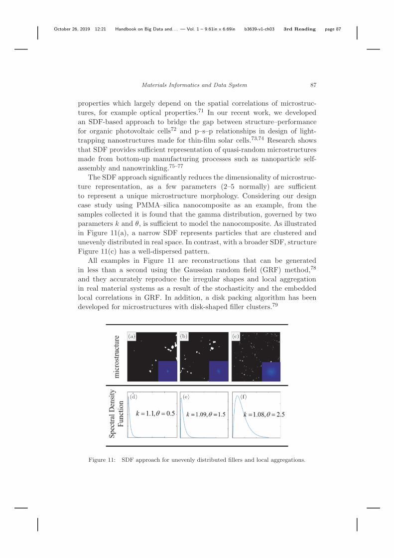
The SDF approach significantly reduces the dimensionality of microstruc-ture representation, as a few parameters (2–5 normally) are sufficientto represent a unique microstructure morphology. Considering our designcase study using PMMA–silica nanocomposite as an example, from thesamples collected it is found that the gamma distribution, governed by twoparameters k and θ, is sufficient to model the nanocomposite. As illustratedin Figure 11(a), a narrow SDF represents particles that are clustered andunevenly distributed in real space. In contrast, with a broader SDF, structureFigure 11(c) has a well-dispersed pattern.
All examples in Figure 11 are reconstructions that can be generatedin less than a second using the Gaussian random field (GRF) method,78
and they accurately reproduce the irregular shapes and local aggregationin real material systems as a result of the stochasticity and the embeddedlocal correlations in GRF. In addition, a disk packing algorithm has beendeveloped for microstructures with disk-shaped filler clusters.79
Figure 11: SDF approach for unevenly distributed fillers and local aggregations.

October 26, 2019 12:21 Handbook on Big Data and. . . — Vol. 1 – 9.61in x 6.69in b3639-v1-ch03 3rd Reading page 88
88 W. Chen et al.
In the design case study shown in Section 7, the SDF representation isused to rapidly generate samples of microstructures and create metamodelsof s–p relationships for a wide range of microstructural designs.
3.4. Machine learning-based MCR techniques
Though not implemented yet in NanoMine, a few state-of-the-art machinelearning methods for MCR are briefly introduced here. Their ability to modelhighly nonlinear functions with nominal user input, coupled with speedand flexibility make them an attractive proposition. These methods can becategorized as follows:
(a) Supervised learning80,81: Using a single 2D/3D microstructure sampleas a training dataset, a decision tree is used to learn the conditional prob-ability distribution of any individual pixel’s value given its surroundingpixel phases. Reconstruction consists of taking a realization from thelearned model, and rendering the method cost-effective and applicableto a wide range of material systems.
(b) Instance-based learning37,82: This approach uses a large database of2D/3D microstructures to search for an instance that is most similar(using predefined similarity metric) to the microstructure under con-sideration. Thus, the reconstruction procedure is essentially a rigoroussearch through the database.
(c) Deep learning83–85: This technique employs hierarchies of stacked neu-ral network layers that encode implicit features into hyper-dimensionalspaces through linear multiplications and nonlinear transformations.
The above techniques have shown success in characterization and recon-struction of polymer nanocomposite systems. However, the potential of thesemachine learning techniques for materials design is still being explored. Onechallenge is the lack of explicit description of microstructure design variablesand their physical relationships with processing conditions.
4. Dimension Reduction and Machine Learningof P–S–P Relationships
To manage the dimensionality of microstructure design representation, datamining and supervised learning techniques have been employed for dis-covering important microstructure features and determining microstructuredesign variables. Recent work has achieved microstructure dimensional-ity reduction via manifold learning37 and kernel principal components.86
October 26, 2019 12:21 Handbook on Big Data and. . . — Vol. 1 – 9.61in x 6.69in b3639-v1-ch03 3rd Reading page 89
Materials Informatics and Data System 89
However, unsupervised learning methods that rely on image data only donot capture the impact of microstructure on material properties, so that thereduced parameter set may not be suitable for the purpose of material design.Limited efforts have been made towards modeling the microstructure–property relationship using statistical learning and further reducing thehigh dimensionality of microstructure features obtained from microscopicimages.
There are two common types of dimension reduction techniques inmachine learning: feature selection and feature extraction. “Feature selection”reduces the number of variables in a system by selecting a subset of relevantfeatures, while “feature extraction” projects the original high-dimensionalfeature space into a reduced space. Both selection and extraction can beeither supervised or unsupervised. The projection incurred in extractionmethods usually refers to a linear or nonlinear transformation of the originalvariables. Extraction methods are not suitable when the physical meaning ofthe original variables needs to be preserved. Feature selection, on the otherhand, chooses a subset of more informative features from the original setand fits many design requirements. A supervised ranking method based onthe Relief algorithm17 has been developed in our earlier work to rank theimportance of microstructure descriptors. However, the method does notaddress the redundancy among descriptors and it is also quite subjective indetermining how many descriptors to keep from a ranked list.
We present here an structural equation modeling-based approach18 thatcombines feature selection and feature extraction techniques for uncover-ing latent microstructure features. SEM is a multi-variate data analysismethod often used in social science for problems with latent layers andpath structures.87 We view microstructures as observations of underlyingstructural characteristics and apply a measurement model in SEM torepresent the relationship as shown in Figure 12. By introducing latentlayers (structural features) in mapping input and output relationships, weare able to identify the relationships and dependencies among differentmicrostructure descriptors. The whole procedure consists of two main parts.First, exploratory factor analysis (EFA)88 is used to reduce the number ofdescriptors as a part of feature selection. Second, for feature extraction, theoriginal descriptors are grouped under a few latent factors, and each latentfactor is linked to a set of descriptors (called indicators). The extractedlatent factors can be considered categories of microstructure features,and the grouped structure reflects the correlation patterns of descriptors.Depending on data availability, responses in an SEM structure may include

October 26, 2019 12:21 Handbook on Big Data and. . . — Vol. 1 – 9.61in x 6.69in b3639-v1-ch03 3rd Reading page 90
90 W. Chen et al.
Figure 12: SEM-based learning (X and Y represent observed inputs and outputs, F andF ′ indicate latent factors associated with X and Y , respectively).
a microstructure correlation function (CF) or material properties, whichare used to identify the underlying descriptor–CF or descriptor–propertyrelationship. With the identified structure, the partial least square (PLS)technique89 is employed to estimate the coefficients in SEM modeling; thecoefficients represent the influences of descriptors.
By building an SEM model, we are able to deal with high correlationsamong all candidate descriptors, gain more insight into their relationships,and identify latent factors (e.g., under categories of “composition”, “geome-try”, and “dispersion”) for categorizing microstructure features. In Ref. [18],for epoxy-silica microstructures, four descriptors, volume fraction, clustersize, nearest neighbor distance, and cluster roundness, are found to besignificant through the SEM analysis using CF as the response (image dataonly). The sufficiency of these descriptors is validated through confirmationof the correlation function of the reconstructed images using the reduceddescriptors versus the original one.
Once the reduced dimensionality is determined, machine learning toolsare widely used for establishing metamodels of s–p relationships or p–srelationships using available data. Figure 13 illustrates the metamodelscreated between microstructure key descriptors and permittivity for anepoxy-silica system18 based on finite element simulations. As shown, smallercluster size and larger volume fraction of silica lead to a better dielectricperformance: higher energy storage capability (high ε′) and smaller dielectricloss (small tan δ) of the epoxy-silica system. This observation is consistentwith the findings in the literature that systems with small particles have high

October 26, 2019 12:21 Handbook on Big Data and. . . — Vol. 1 – 9.61in x 6.69in b3639-v1-ch03 3rd Reading page 91
Materials Informatics and Data System 91
Figure 13: Structure–property relationship. Linear relationship between dielectric prop-erties and key descriptors, only volume fraction and cluster size are considered forvisualization.
surface area-to-volume ratio, which is critical in determining the propertiesof nanofilled materials.90 In general cases, the s–p relationship can be morecomplicated so we may need to fit nonlinear models, such as Gaussian process(GP) models.
5. Descriptor-based Processing–Structure Modelingof PMMA–Silica System
To date, polymer nanocomposites have demonstrated outstanding propertiesand played a significant role in scientific discoveries.21,63,91–96 However,their commercial use is very limited due to the difficulty of processingsuch materials on a commercial scale with control over the morphology.More specifically, because a quantitative p–s–p relationship is lacking, toobtain the optimized material property,61,97–99 one has to tailor nanoparticledispersion by controlling the processing conditions in a trial-and-errormanner.100,101 It is crucial to develop a quantitative modeling approachwhich can incorporate the particle/surface chemistry and processing requiredto achieve a specific nanofiller dispersion. Such a quantitative modelwill provide more in-depth understanding of nanocomposites and greatlyaccelerate the design and optimization of advanced materials. In this section,we present a descriptor-based approach for creating p–s relationships undernon-equilibrium processing conditions. Three separate steps are involved:processing quantification, microstructure characterization, and processing–structure relationship development.

October 26, 2019 12:21 Handbook on Big Data and. . . — Vol. 1 – 9.61in x 6.69in b3639-v1-ch03 3rd Reading page 92
92 W. Chen et al.
5.1. Quantification of processing conditions
Processing is usually complex. Typically, for each individual processingtechnique, there are many processing conditions and settings to be tweakedto achieve optimized material properties. Since some of the processingparameters are correlated and some do not have significant impact inmicrostructure dispersion, it is of great importance to select the proper setof parameters to represent the most significant aspects of processing thatcontributes to the dispersion. To this end, we extend the representativeparameters for equilibrium conditions to the ones for non-equilibriumsystems by adding a processing energy descriptor.
Prior work100–102 in developing processing–structure relationships fornanocomposites primarily considered two different aspects. (1) The firstaspect is how the surface chemistry of nanoparticles controls filler dispersion.For instance, Natarajan et al.102 developed a quantitative relationshipbetween interfacial energy and dispersion. The filler is found to be well-dispersed when the filler and the polymer matrix are thermodynamicallycompatible. Agglomeration increases when the work of adhesion betweenthe fillers exceeds the work of adhesion between the filler and the polymer.Villmow et al.100 found that the surface energy also determines the mobilityof the interphase, which significantly contributes to material properties suchas glass transition temperature. (2) In contrast, the second aspect of researchstudies how processing energy (e.g., specific processing energy input) affectsthe filler dispersion. For instance, Kasaliwal et al.101 discovered a power lawrule for the dependence of the dispersion of CNT agglomerates on the specificprocessing energy applied.
While the aforementioned studies provide either qualitative or quan-titative results for developing p–s relationships, they consider only thesurface energy or the processing energy independently. For non-equilibriumprocessing methods, we consider the two processing energy parameterssimultaneously: interphase energy and processing energy. Before we formallyillustrate the formation of these two energy parameters, we confine thefactors that potentially contribute to dispersion. Generally, non-equilibriumprocessing covers a wide range of processing techniques that result inkinetically trapped microstructures. The most popular one in industrialapplications is extrusion because it is inexpensive, fast, and simple. Priorqualitative study has found that to reduce the nanoparticle agglomeratesize, the agglomerate cohesive strength must be overcome. With increasingshear energy input, the agglomerate size can be further reduced. Several

October 26, 2019 12:21 Handbook on Big Data and. . . — Vol. 1 – 9.61in x 6.69in b3639-v1-ch03 3rd Reading page 93
Materials Informatics and Data System 93
components would be involved in the processing of particle deagglomera-tion101,103–107:
1. Incorporation of the filler into the matrix.2. Wetting of the filler with matrix material.3. Infiltration of the matrix into the agglomerate.4. Breaking up of the agglomerates and erosion of nanoparticles from the
agglomerate surface.5. Distribution within the matrix.6. Reagglomeration due to particle collisions during mixing.
These processes are dependent on nine factors:
1. Surface energies of the components;2. Viscosity of the polymer;3. Packing density of the agglomerate;4. Chain stiffness of the polymer;5. Shear stress;6. Specific energy input during processing;7. Agglomerate size;8. Crystallinity;9. Agglomerate strength.
Extensive research101,108–113 has been carried out on the quantitativedependence of some of the listed processes and factors. We encourage readersto refer to this literature for detailed explanations of the dependencies. Inquantifying the processing conditions in extrusion, we consider four out ofthe nine factors: surface energy, polymer viscosity, shear stress, and specificprocessing energy input (factors 1, 2, 5 and 6). The other factors are ignoredin this study either because of the limited number of composite systemsin the study (e.g., factors 4 and 8) or difficulty in gaining the neededinformation during the applied process (e.g., for studying factors 3 and 5).For the demonstration example in this section, we narrow our discussion tothe simplest extrusion method, single-screw extrusion as used in Ref. [25]and the corresponding dataset in Refs. [25 and 114]. Data collected fromexperiments has been curated and stored in NanoMine.
We consider silica nanoparticles (15 nm diameter) as a filler that is surfacemodified using three monofunctional silanes by the method elucidated byNatarajan et al.102 The silanes were differentiated by the end group of themolecule — octyldimethylmethoxysilane, chloropropyldimethylethoxysilane,and aminopropyldimethylethoxysilane. The polymer matrices of polystyrene,

October 26, 2019 12:21 Handbook on Big Data and. . . — Vol. 1 – 9.61in x 6.69in b3639-v1-ch03 3rd Reading page 94
94 W. Chen et al.
polypropylene, and PMMA were used in powder form for the extrusionprocess. Each combination of surface modification and polymer matrixprovides a range of interfacial energy interactions.115 Functionalized particleswere precipitated using an antisolvent, mixed with the polymer matrixpowder, and dried to produce a particle–polymer powder mixture, asexplained by Hassinger et al.25
Prior to extrusion, the polymer–particle powders were jet milled to reducethe size of powder particles. The powders were fed into a single screwextruder, with screw diameter of 12.7 mm, screw length of 342.9 mm, andchannel width of 9.8 mm. Extrusion was carried out at 180◦C and at varyingscrew speeds (20, 100, and 195 RPM) to examine the influence of processingparameters on the final dispersion state of the particles. More detaileddescriptions of the processing can be found in Ref. [25].
5.2. Interfacial energy descriptor
The final dispersion state depends on deagglomeration and reagglomerationof the nanoparticles during processing. The simulation by Starr et al.116
shows that when the particle–polymer interaction is weaker than theparticle–particle interaction, the particles agglomerate abruptly. Herein, weadopt Natarjan et al.102 and Khoshkava et al.’s117 quantification of theseinteractions — the ratio of the work of adhesion between filler and polymerand the work of adhesion of filler to filler (denoted as WPF/WFF) to representthe interfacial interactions. Table 3 lists the values of the interfacial energydescriptor, WPF/WFF, for all the composites in the dataset. The cells of thecompatible combinations are marked in gray.
5.3. Processing energy descriptor
The other descriptor that we introduce is the processing energy descriptor,which essentially measures the energy consumption within the screw during
Table 3: Descriptors describing the interfacial energy ofthe various material combinations.
Silica modification Polymer PP PS PMMA
Octyl-mod-silica WPF/WFF 0.94 1.15 1.12Chloro-mod-silica WPF/WFF 0.84 1.04 1.05Amino-mod-silica WPF/WFF 0.78 0.95 0.96
Note: The compatible combinations are given in lightgrey color.

October 26, 2019 12:21 Handbook on Big Data and. . . — Vol. 1 – 9.61in x 6.69in b3639-v1-ch03 3rd Reading page 95
Materials Informatics and Data System 95
processing. We denote the screw channel depth of the extruder as H(L), inwhich H is dependent on the length of the screw L. The screw diameter isdenoted as d, while the screw speed is represented by N . Then the shearrate could be computed by,118
γ =π(d − 2H(L))N
H(L). (8)
Given the viscosity ηP , the shear stress is
τ = ηP · γ. (9)
The viscosity of the nanocomposite can be estimated by first determining theviscosity of the neat polymer using the Cross Law as shown in Equation (10)and then using the Einstein equation for filled polymers as shown inEquation (11). In these equations, ηP and ηF are the viscosities of the neatpolymer and filled polymer, respectively, ηP , lim is the viscosity at infiniteshear rate for the neat polymer, ηP ,0 is the viscosity at zero shear rate forthe neat polymer, α is a fitting-factor, and f is the filler fraction, where theviscosity of the materials could be estimated119:
ηP = ηlim +(ηP,0 − ηP,lim)1 − α · Y 2/3
, (10)
ηF = ηP + f · 2.5 + f · 21.42. (11)
Using Lai’s120 theoretical model, the processing energy consumption in acircular segment with infinitesimal length along the screw length directioncan be calculated as
dw =πDΩ60
dFby , (12)
where D is the screw diameter, Ω is the screw speed, and dFby is the tangentcomponent of the traction on the screw barrel surface (Fby = Sbμbγbcosϕ),in which Sb is the area of traction on the screw barrel, μb is the viscosity ofthe molten polymer and ϕ is the angle between the resultant traction andthe channels. By taking the integral of dw along the length of the screw, thetotal energy consumption, w, is obtained. The processing energy descriptor,namely the energy consumption per mass unit of the throughput, can beobtained by
Eγ =w
qm, (13)
where qm is the throughput.

October 26, 2019 12:21 Handbook on Big Data and. . . — Vol. 1 – 9.61in x 6.69in b3639-v1-ch03 3rd Reading page 96
96 W. Chen et al.
5.4. Microstructure descriptors from characterization
In addition to quantifying the processing conditions, it is also of greatimportance to characterize microstructures with a set of low-dimensionalparameters. A necessary step before microstructure characterization ismaterial phase segmentation. For filler–matrix composites, it is essentially abinarization process that distinguishes fillers from matrix. While the bina-rization of TEM images is typically done by setting a global threshold,34,121
we find it does not work well with the TEM images in our dataset. The majorproblem is that, in our TEM images, local shades or unevenness would resultin a darker/lighter spot in some particular locations, and these spots wouldbe misclassified when a global thresholding algorithm is applied. Therefore,we apply the Niblack algorithm,35 which is a sliding window algorithm thattakes advantage of local pixel statistics to determine the local thresholdingvalue. Figure 14 demonstrates how the Niblack algorithm outperforms theglobal thresholding algorithm, which is clearly seen in the red boxed areawhere particles in a shaded region of the original TEM image are betteridentified using the Niblack method.
While a range of MCR techniques are available as introduced inSection 3,38 the descriptor-based characterization approach15 is used as mostof the clusters are spherical. Per Xu et al.,15 the descriptors considered arelisted in Table 4.
While descriptor-based characterization provides a rich set of physicaldescriptors that represent the microstructures being studied, the dimen-sionality is still too high to be correlated to the two processing descriptorsdiscussed above. Therefore, a supervised learning-based descriptor selection
Figure 14: A demonstration of a sample TEM image with local shades/unevenness(a) and a comparison between the global thresholding algorithm (b) and Niblackalgorithm35 (c).
October 26, 2019 12:21 Handbook on Big Data and. . . — Vol. 1 – 9.61in x 6.69in b3639-v1-ch03 3rd Reading page 97
Materials Informatics and Data System 97
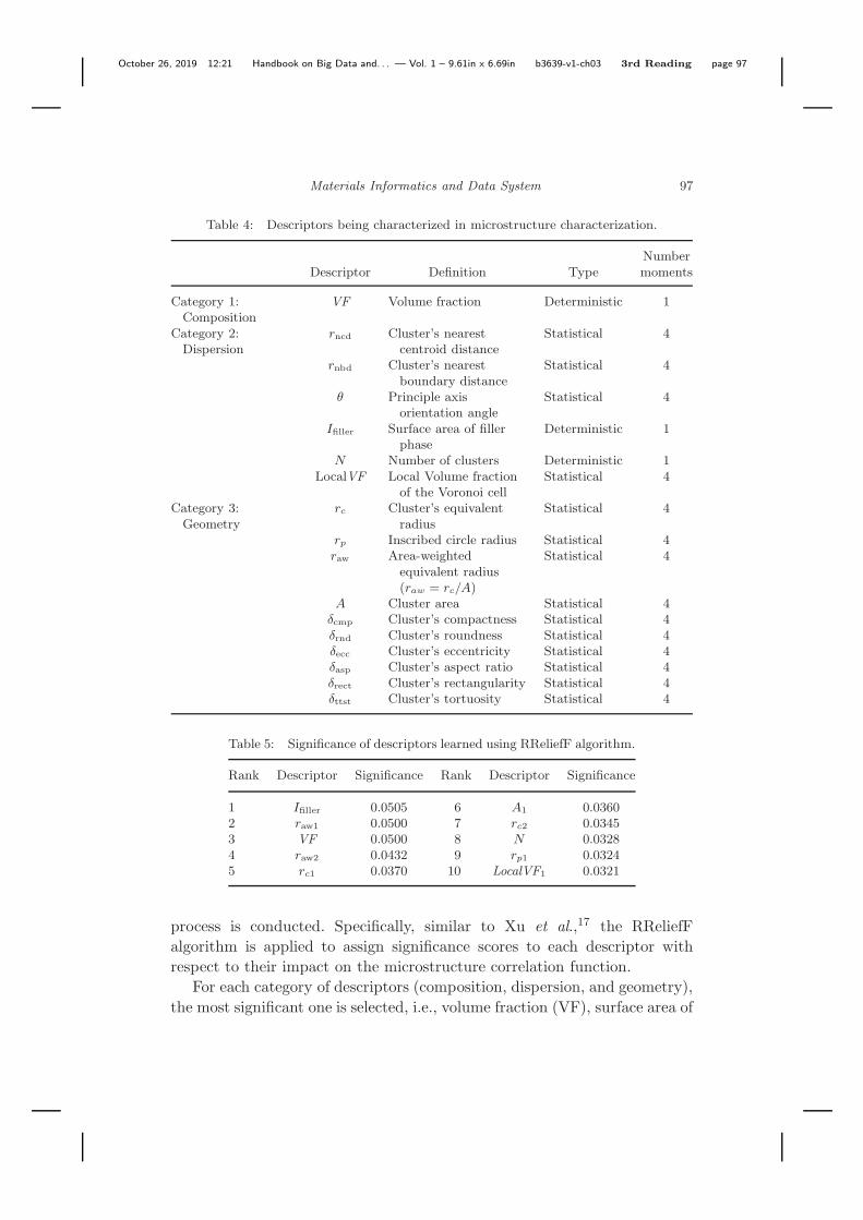
Table 4: Descriptors being characterized in microstructure characterization.
NumberDescriptor Definition Type moments
Category 1:Composition
VF Volume fraction Deterministic 1
Category 2:Dispersion
rncd Cluster’s nearestcentroid distance
Statistical 4
rnbd Cluster’s nearestboundary distance
Statistical 4
θ Principle axisorientation angle
Statistical 4
Ifiller Surface area of fillerphase
Deterministic 1
N Number of clusters Deterministic 1LocalVF Local Volume fraction
of the Voronoi cellStatistical 4
Category 3:Geometry
rc Cluster’s equivalentradius
Statistical 4
rp Inscribed circle radius Statistical 4raw Area-weighted
equivalent radius(raw = rc/A)
Statistical 4
A Cluster area Statistical 4δcmp Cluster’s compactness Statistical 4δrnd Cluster’s roundness Statistical 4δecc Cluster’s eccentricity Statistical 4δasp Cluster’s aspect ratio Statistical 4δrect Cluster’s rectangularity Statistical 4δttst Cluster’s tortuosity Statistical 4
Table 5: Significance of descriptors learned using RReliefF algorithm.
Rank Descriptor Significance Rank Descriptor Significance
1 Ifiller 0.0505 6 A1 0.03602 raw1 0.0500 7 rc2 0.03453 VF 0.0500 8 N 0.03284 raw2 0.0432 9 rp1 0.03245 rc1 0.0370 10 LocalVF1 0.0321
process is conducted. Specifically, similar to Xu et al.,17 the RReliefFalgorithm is applied to assign significance scores to each descriptor withrespect to their impact on the microstructure correlation function.
For each category of descriptors (composition, dispersion, and geometry),the most significant one is selected, i.e., volume fraction (VF), surface area of

October 26, 2019 12:21 Handbook on Big Data and. . . — Vol. 1 – 9.61in x 6.69in b3639-v1-ch03 3rd Reading page 98
98 W. Chen et al.
filler phase (Ifiller), and area weighted equivalent radius (raw1), respectively.We also find that these three descriptors are linearly correlated. Therefore,we further condense them into one integrated descriptor — volume fractionnormalized filler surface area (Ifiller = Ifiller/VF).
5.5. Building processing–structure relationships
Table 6 summarizes the values of the processing descriptors and microstruc-ture descriptors presented above. The impact of each processing descriptoron the microstructure descriptor is first studied. Then a predictive p–s modelis established by mapping the two sets of descriptors.
First, consider the impact of interfacial energy on the microstructuredescriptor. Recall that a larger value of Ifiller indicates better dispersion. Thematerials with the best compatibility (e.g., highest values of WPF/WFF) showthe best dispersion (octyl-modified silica and PS) (Figure 15) as indicatedby the largest normalized interface area.
The microstructure dispersion descriptor Ifiller also depends on theprocessing energy descriptor Eγ (Figure 16). In Figure 16, samples with thesame type of polymer and surface modification method are grouped togetherand marked with the same symbol. Figure 16 shows that the dispersion of thesamples with the same polymer and surface modification could be improvedby increasing the processing energy.
Table 6: Descriptor values of the composites samples.
Polymer Particle surface modification WPF/WFF Eγ (J/g) Ifiller
PS Octyl 1.15 34.52 0.2085.73 0.21
Chloro 1.04 33.18 0.1585.66 0.17
Amino 0.95 33.28 0.12104.34 0.1285.76 0.12
PP Octyl 0.94 0.65 0.163.03 0.13
Chloro 0.84 0.58 0.073.53 0.17
Amino 0.78 0.65 0.092.16 0.123.08 0.12
PMMA Amino 0.96 103.10 0.11964.16 0.13410.92 0.12

October 26, 2019 12:21 Handbook on Big Data and. . . — Vol. 1 – 9.61in x 6.69in b3639-v1-ch03 3rd Reading page 99
Materials Informatics and Data System 99
0.75 0.8 0.85 0.9 0.95 1 1.05 1.1 1.15 1.20.06
WPF
/WFF
0.08
0.1
0.12
0.14
0.16
0.18
0.2
0.22
PSPPPMMAW
PF/W
FF=1
I fill
er
Figure 15: The impact of the filler–matrix compatibility descriptor (WPF/WFF) on themicrostructure dispersion (Ifiller). The dashed line indicates the threshold of 1, beyondwhich materials have a wetting angle of 0◦ and the particles wet the polymer.
Natarajan et al.,102 who used solvent mixing, found a very abruptaggregation of nanoparticles when the compatibility of the nanoparticleswith the polymer matrix goes from compatible (e.g., WPF/WFF ≥ 1) to notcompatible (e.g., WPF/WFF < 1). The results in this research show thatthe aggregation of the nanoparticles with a WPF
WFF< 1 is less abrupt than
was found by Natarajan et al. for solvent mixed nanocomposites.102 This isbecause the materials that are melt processed are not at equilibrium andthe mixing energy and fast cooling prevents aggregation, while for Natarjanet al. the samples were annealed to a state of quasi-equilibrium.102
These results indicate that dispersion quality, Ifiller, can be correlated toboth the material compatibility (WPF/WFF) and the processing energy (Eγ).The relationship between these variables was further developed using datamining techniques to provide a mathematical expression, which could beused in further analyses and prediction schemes. The results for the threetypes of polymer matrix are shown in Figure 17, where the R2 values indicatethat Ifiller is linearly correlated with the combined energetic terms.
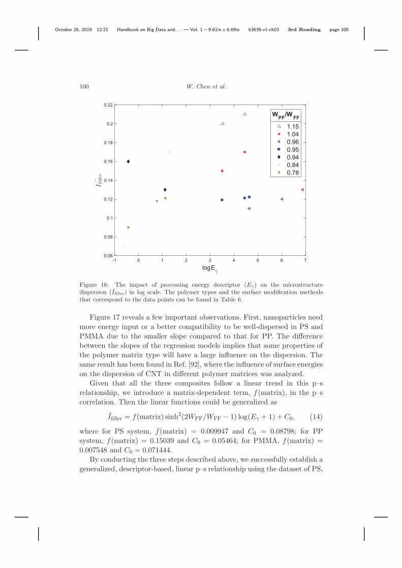
October 26, 2019 12:21 Handbook on Big Data and. . . — Vol. 1 – 9.61in x 6.69in b3639-v1-ch03 3rd Reading page 100
100 W. Chen et al.
0 1 2 3 4 5 6 7-1
logE
0.06
0.08
0.1
0.12
0.14
0.16
0.18
0.2
0.22
1.151.040.960.950.940.840.78
WPF
/WFF
Figure 16: The impact of processing energy descriptor (Eγ) on the microstructuredispersion (Ifiller) in log scale. The polymer types and the surface modification methodsthat correspond to the data points can be found in Table 6.
Figure 17 reveals a few important observations. First, nanoparticles needmore energy input or a better compatibility to be well-dispersed in PS andPMMA due to the smaller slope compared to that for PP. The differencebetween the slopes of the regression models implies that some properties ofthe polymer matrix type will have a large influence on the dispersion. Thesame result has been found in Ref. [92], where the influence of surface energieson the dispersion of CNT in different polymer matrices was analyzed.
Given that all the three composites follow a linear trend in this p–srelationship, we introduce a matrix-dependent term, f(matrix), in the p–scorrelation. Then the linear functions could be generalized as
Ifiller = f(matrix) sinh2(2WPF/WFF − 1) log(Eγ + 1) + C0, (14)
where for PS system, f(matrix) = 0.009947 and C0 = 0.08798; for PPsystem, f(matrix) = 0.15039 and C0 = 0.05464; for PMMA, f(matrix) =0.007548 and C0 = 0.071444.
By conducting the three steps described above, we successfully establish ageneralized, descriptor-based, linear p–s relationship using the dataset of PS,
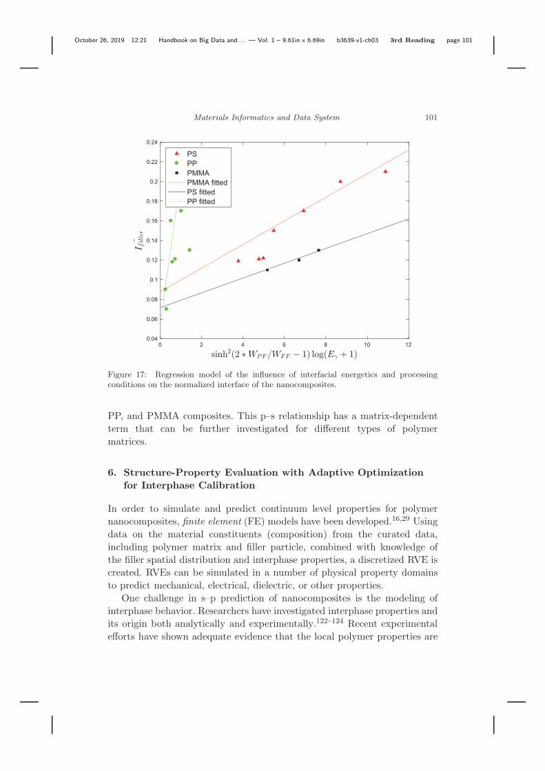
October 26, 2019 12:21 Handbook on Big Data and. . . — Vol. 1 – 9.61in x 6.69in b3639-v1-ch03 3rd Reading page 101
Materials Informatics and Data System 101
0 2 4 6 8 10 120.04
0.06
0.08
0.1
0.12
0.14
0.16
0.18
0.2
0.22
0.24
PSPPPMMAPMMA fittedPS fittedPP fitted
Figure 17: Regression model of the influence of interfacial energetics and processingconditions on the normalized interface of the nanocomposites.
PP, and PMMA composites. This p–s relationship has a matrix-dependentterm that can be further investigated for different types of polymermatrices.
6. Structure-Property Evaluation with Adaptive Optimizationfor Interphase Calibration
In order to simulate and predict continuum level properties for polymernanocomposites, finite element (FE) models have been developed.16,29 Usingdata on the material constituents (composition) from the curated data,including polymer matrix and filler particle, combined with knowledge ofthe filler spatial distribution and interphase properties, a discretized RVE iscreated. RVEs can be simulated in a number of physical property domainsto predict mechanical, electrical, dielectric, or other properties.
One challenge in s–p prediction of nanocomposites is the modeling ofinterphase behavior. Researchers have investigated interphase properties andits origin both analytically and experimentally.122–124 Recent experimentalefforts have shown adequate evidence that the local polymer properties are
October 26, 2019 12:21 Handbook on Big Data and. . . — Vol. 1 – 9.61in x 6.69in b3639-v1-ch03 3rd Reading page 102
102 W. Chen et al.
significantly altered in the vicinity of polymer surface, through measuring thelocal mechanical properties and by correlating thin film and nanocompositedata.125,126 Given the limitations of direct measurements of interphaseproperties in the experiments, one approach to calculate the interphaseproperties is inversely through tuning the parameters in micro-scale modelconstitutive equations or finite element analysis using the bulk propertiesfrom experiments.28,127,128
It has been shown in our early work28,29,129 that the interphase propertiescan often be described by shifting factors based on the pure matrixproperties, which can be represented by a Prony Series as a parameterfunction of multiple relaxation and times and strengths. The interphaseproperties in those models can be obtained through a trial-and-error-based iterative tuning procedure by matching the simulations given specificexperimental data. However, the trial-and-error-based tuning process canbe very time-consuming given the complexity of experimental data andsimulation cost of FEA.
We present here an automated optimization method to solve the inversecalibration problems. More details about this approach can be found inour previous paper.26 Using a library of composite-level FE simulations,key interface modeling parameters (shift factors) are determined to matchexperimental properties. An adaptive sampling approach is implementedin searching for the unknown interphase modeling parameters, and themethod has been tested on both dielectric and viscoelastic interphaseproperties. The interphase properties are assumed to be well-representedby the shifting factors with respect to matrix properties. Therefore, theoptimization objective is to find the shifting factors that will optimallymatch the experimental data through applying adaptive optimization. Thekey component of our approach is summarized in Figure 18.
(1) Based on our previous understanding of the interphase, empirical boundsof shifting factors are applied to set the range to sample initial trainingshifting factors using optimal Latin hypercube (OLHC). The FEA modelis run using each set of shifting factors to obtain a simulation result. Theobjective function is formulated as the difference between the simulationand experimental result using mean square error (MSE).
(2) A GP model is applied to fit the metamodel that correlates theobjective function (difference F) with features (shifting factors), withuncertainties.

October 26, 2019 12:21 Handbook on Big Data and. . . — Vol. 1 – 9.61in x 6.69in b3639-v1-ch03 3rd Reading page 103
Materials Informatics and Data System 103
Figure 18: The automated adaptive optimization strategy for searching the interphaseproperties: (1) FEA is run on each point in the initial shift factor set from DOE andthen processed to formulate our objective function by calculating the difference betweensimulated results and experiments using MSE; (2) a GP model is applied to construct thesurrogates for predicting the value of objective function (difference F) within the designspace; (3) EI chooses the best candidate points for additional simulation.
(3) Based on the fitted metamodel, new candidate points for the calibrationparameters are selected based on feedback from the surrogate model bycalculating the expected improvement (EI).130–132
This process is usually identified as an adaptive optimization process, alsocalled Bayesian optimization, which augments the training shifting factorsets and drives the subsequent iterative improvement of the surrogate modeland prediction accuracy. The adaptive optimizer is applied to construct thesurrogate model and suggest the next optimal sampling points in order tominimize the difference between the experiments and simulations and returnthe optimal solution iteratively.
Using this automated approach and given the target experimental data,the interphase properties on dielectric and viscoelastic studies can bedetermined automatically. Taking a representative dielectric dataset (fora nanocomposite composed of 2 wt.% bimodal anthracene–PGMA graftedsilica in epoxy133,134), the method is shown to estimate the interphaseproperties with only tens of iterations as shown in Figure 19. The predictionaccuracy at each step is evaluated by calculating the discrepancy betweenthe simulated data using the predicted shifting factor from the adaptiveoptimizer and the given experimental properties using MSE. As the iteration

October 26, 2019 12:21 Handbook on Big Data and. . . — Vol. 1 – 9.61in x 6.69in b3639-v1-ch03 3rd Reading page 104
104 W. Chen et al.
Figure 19: Evolving of optimal solution as a function of successive iterations: (a) thediscrepancy between the optimal prediction and the experimental data as a function ofiterations; (b) comparison between experimental data and the simulated result using thepredicted interphase properties given from the adaptive optimizer.
proceeds, the discrepancy keeps decreasing (though not monotonically, likelydue to the model uncertainties) indicating an increase in model accuracy asnew sampling points are added based on maximum EI.
Ideally, minimal discrepancy between simulated and experimental dataacross the entire frequency band is desired and should lead to well-matcheddata curves. Practically, we find a threshold value C, indicating an acceptable

October 26, 2019 12:21 Handbook on Big Data and. . . — Vol. 1 – 9.61in x 6.69in b3639-v1-ch03 3rd Reading page 105
Materials Informatics and Data System 105
fit between the experimental data and simulated results. C may varydepending the specific applications, but for our case C is set as 0.01.The iteration stops after the difference is smaller than the threshold. Whilethe threshold is met at iteration 20, we plot more iterations in order toshow the convergence of our adaptive optimization procedure.
Figure 20: Comparison of matrix, interphase, and composite properties for 2 wt.%bimodal anthracene–PGMA grafted silica in epoxy.

October 26, 2019 12:21 Handbook on Big Data and. . . — Vol. 1 – 9.61in x 6.69in b3639-v1-ch03 3rd Reading page 106
106 W. Chen et al.
By applying the adaptive optimizer above, the optimal shifting factorsthat achieve a good match with experimental data can be determined.Because the interphase shifting factors are the descriptors for the interphaseproperties and completely define those properties, the interphase propertiesare thus determined. It is important to note that without experimentalverification of these local properties, these represent a reasonable approx-imation to the actual interphase properties. Figure 20 shows the optimalinterphase properties together with the matrix and composite properties.The interphase properties determined are significantly different from thatof the matrix. This property difference is expected due to mobility changesof polymer chains near the particles causing changes in the local physicalproperties such as dielectric spectra of the polymer. For this sample,the interphase region shows a higher permittivity and loss comparedwith matrix and composite data. This interphase property agrees withthe experimental data where the addition of functional groups on fillersenhances the relative permittivity.133 Further work is needed to determinepredictive models for the interphase parameters based on sufficiently detailedexperimental data.
7. Processing–Structure–Property Integration for Designof Nanodielectric Materials in Capacitors
In this section, the capacitor design problem is used as an example todemonstrate the design of nanodielectric materials by integrating p–s ands–p relationships presented in the earlier sections. Capacitor design is amulti-objective optimization problem where the objectives of maximizingdielectric constant and minimizing its dielectric loss need to be achievedsimultaneously. Dielectric constant, also known as permittivity, affectsthe energy storage capability of capacitors. Dielectric loss quantifies adielectric material’s inherent dissipation of electromagnetic energy (e.g.,heat). Increasing dielectric constant often results in dielectric loss. Multi-criteria optimization technique will be used to make the trade-off betweencompeting design objectives.
The remainder of this section is organized as follows. Section 7.1introduces the silica-PMMA- material system and the formulation ofcapacitor design optimization. Section 7.2 provides details of the s–pmodeling, along with the multi-criteria microstructure optimization results.In Section 7.3, the optimized structure is mapped to processing condi-tions based on descriptor-based processing–structure mapping presented inSection 5.

October 26, 2019 12:21 Handbook on Big Data and. . . — Vol. 1 – 9.61in x 6.69in b3639-v1-ch03 3rd Reading page 107
Materials Informatics and Data System 107
7.1. Capacitor design case study
The material system of interest is PMMA/amino-modified silica nanocom-posites with silica loading up to 5%. This model system is chosen because wehave collected significant data for calibration and validation. The inclusion ofsilica in PMMA influences the overall permittivity and dielectric loss of thecomposites, and the dispersion quality of silica determines the strength ofthe effects. PMMA and silica are mixed using a twin screw extruder, and thehigh processing input energies tend to make the fillers more evenly dispersedin the polymer matrix.
The key property of a capacitor is the maximum energy, E it can store,which is determined by the following equation:
E =12εAdU2
d , (15)
where ε and Ud are the permittivity and dielectric breakdown strength of thedielectric material, A is the area of the plate in a parallel plate capacitor,and d is the gap thickness containing the dielectric material. Since we aredesigning the material, the geometry parameters A and d of the capacitor arenot of interest. The breakdown of nanodielectrics is a complex phenomenonand the FEA simulation model is still under development. Therefore, inthis case study, we assume the breakdown strength Ud is constant and onlyconsider the permittivity as a major design target for maximizing energystorage.
Another important property in capacitor design is dielectric loss, whichessentially quantifies the amount of heat generated during the charging anddischarging process. Dielectric loss is usually represented by loss tangent,and is also known as dissipation factor (DF), and is given by
tan δ = DF =ε′′
ε′, (16)
where ε′′ and ε′ are the imaginary part and real part of the dielectricmaterials’ permittivity. Lower loss tangent is desired to avoid significantenergy loss during the usage of the capacitor.
In this case study, the microstructure of the composites is optimized basedon FEM-based s–p relationships (Section 6) first and then the empirical p–srelationship (Section 5) is used to find the optimal processing conditions.The mathematical formulation of this multi-objective optimization problembecomes
minsεS
−E, tan δ, (17)
October 26, 2019 12:21 Handbook on Big Data and. . . — Vol. 1 – 9.61in x 6.69in b3639-v1-ch03 3rd Reading page 108
108 W. Chen et al.
where s represents the microstructure to optimize, and S is the set of allfeasible microstructures. Using the physical-descriptor-based MCR approachintroduced in Section 3, the microstructure representation can be reduced toa small number of design variables (descriptors) d. The above problem canbe reformulated as a simple bounded optimization
mind
−E, tan δ; s.t. dL ≤ d ≤ dU , (18)
where dL and dU are the lower and upper bounds of design variables. Onecommon way to deal with multiple objectives in optimization is to usethe weighted sum of those objectives as a single objective. If using multi-criteria optimization, the Pareto frontier135 is identified to form a set ofnon-dominated solutions based on the trade-off between multiple objectives.Genetic algorithms (GAs)135 have been used widely to find the Paretosolutions.
7.2. Nanodielectric microstructure optimization based
on s–p relationship
The FE-based approach as introduced in Section 6 is used to build predictives–p models. Three major steps are followed:
(1) Use SDF parameters θ and VF as design variables to generate optimalDOE sample points;
(2) Apply the GRF-based algorithm78 to reconstruct microstructures basedon the parameters generated in step (1);
(3) Evaluate the properties of microstructures reconstructed in step (2)using FEA simulation models discussed in Section 6.
It is worth noting here that the normalized filler surface area, Ifiller, which hasbeen found to be the critical structure descriptor in p–s mapping as shown inSection 5, is not directly used as a design variable in our problem. Instead, weuse the parameter of SDF distribution as one design variable. As explainedin Section 3.3, SDF representation provides significant dimension reductionin microstructural analysis and design. Its applicability is also confirmed byimage analysis on the material samples made from the processing techniqueadopted. By analyzing the microstructures of the PMMA-silica system(Figure 21), the SDFs are found to be close to Gamma distribution with
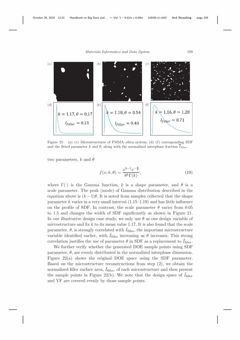
October 26, 2019 12:21 Handbook on Big Data and. . . — Vol. 1 – 9.61in x 6.69in b3639-v1-ch03 3rd Reading page 109
Materials Informatics and Data System 109
Figure 21: (a)–(c) Microstructures of PMMA–silica system; (d)–(f) corresponding SDFand the fitted parameter k and θ, along with the normalized interphase fraction Ifiller.
two parameters, k and θ
f(x; k, θ) =xk−1e−
xθ
θkΓ(k), (19)
where Γ(·) is the Gamma function, k is a shape parameter, and θ is ascale parameter. The peak (mode) of Gamma distribution described in theequation above is (k− 1)θ. It is noted from samples collected that the shapeparameter k varies in a very small interval (1.15–1.19) and has little influenceon the profile of SDF. In contrast, the scale parameter θ varies from 0.05to 1.5 and changes the width of SDF significantly as shown in Figure 21.In our illustrative design case study, we only use θ as one design variable ofmicrostructure and fix k to its mean value 1.17. It is also found that the scaleparameter, θ, is strongly correlated with Ifiller, the important microstructurevariable identified earlier, with Ifiller increasing as θ increases. This strongcorrelation justifies the use of parameter θ in SDF as a replacement to Ifiller.
We further verify whether the generated DOE sample points using SDFparameter, θ, are evenly distributed in the normalized interphase dimension.Figure 22(a) shows the original DOE space using the SDF parameter.Based on the microstructure reconstructions from step (2), we obtain thenormalized filler surface area, Ifiller, of each microstructure and then presentthe sample points in Figure 22(b). We note that the design space of Ifiller
and VF are covered evenly by those sample points.
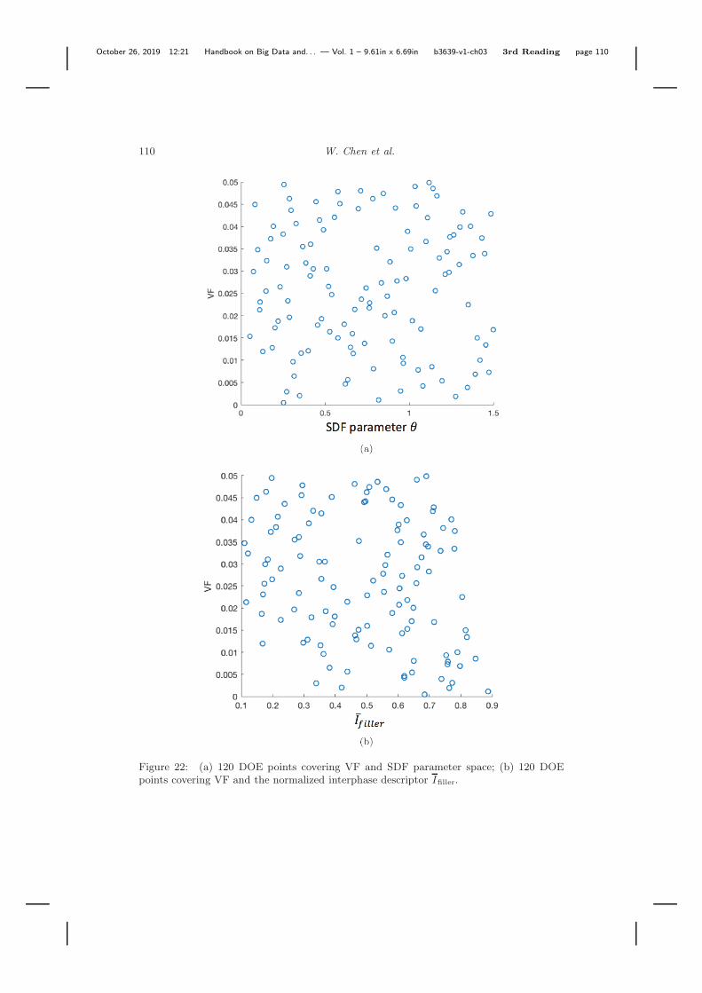
October 26, 2019 12:21 Handbook on Big Data and. . . — Vol. 1 – 9.61in x 6.69in b3639-v1-ch03 3rd Reading page 110
110 W. Chen et al.
Figure 22: (a) 120 DOE points covering VF and SDF parameter space; (b) 120 DOEpoints covering VF and the normalized interphase descriptor Ifiller.
October 26, 2019 12:21 Handbook on Big Data and. . . — Vol. 1 – 9.61in x 6.69in b3639-v1-ch03 3rd Reading page 111
Materials Informatics and Data System 111
After the DOE samples are created over θ and VF, the next step isto evaluate the properties of these samples. The s–p evaluation approachdescribed in Section 6 using physics-based FEA combined with calibratedinterphase parameters is followed. Due to the multiple relaxations observedin the pure matrix, the interphase properties are described using a set of 5Dshifting factors (Mα and Sα for alpha relaxation, Mβ and Sβ for beta relax-ation, and C for the intensity shift of permittivity) related to pure matrixwith the alpha and beta relaxation modeled separately. The interphaseshifting factors are calibrated and obtained inversely by optimally matchinga the composite dielectric spectrum from experimental data for amino-modified silica–PMMA composites via an automated procedure applyingthe adaptive optimization presented in Section 6. Since the composition(filler, matrix, functional group) remains constant for all cases in the DOE,the interphase shifting factors found in this manner can be used for allsimulation predictions in the design study. In the interphase optimizationprocess, multiple microstructural images for each sample are used to obtainthe appropriatre structural descriptors for reconstruction, which is thenused in the optimization procedure. With the interphase properties obtainedfrom the optimization procedure, new microstructure designs are simulatedfollowing the DOE samples to obtain the nanocomposite bulk properties.From the histogram in Figure 23, we can see the simulated permittivityranges from 2.5 to 2.8, and the losses tan δ are roughly in the range of 0.04–0.063. The distribution of permittivity is close to normal distribution butslightly right skewed. The dielectric loss has a highly skewed distributionwith concentrations in small values.
Based on the simulation samples, machine learning techniques areused to build metamodels to replace the expensive s–p simulations. Onecommon technique applied to approximate expensive computer models isthe GP regression model,136 which is a non-parametric statistical model thatcaptures nonlinear response surfaces and provides flexibility for assessinguncertainties in prediction.
A GP y(x) is defined by its mean function m(x) and covariance functionk(xx′):
m(x) = E[y(x)], (20)
k(x,x′) = E[(y(x) − m(x))(y(x′) − m(x′))], (21)
where the vector x indicates the spatial location, and the response y at eachlocation x follows the multi-variate normal distribution:
y(x) ∼ N(m(x), k(x,x′)). (22)

October 26, 2019 12:21 Handbook on Big Data and. . . — Vol. 1 – 9.61in x 6.69in b3639-v1-ch03 3rd Reading page 112
112 W. Chen et al.
Figure 23: (a) Histogram of the simulated permittivity at 1Hz; (b) histogram of simulatedloss tan δ at 1Hz.
For simplicity, the mean function is chosen to be equal to zero and thecovariance function is in the squared exponential form, also known asKriging137:
k(xx′) = σ2 exp(−w(x − x′)2), (23)

October 26, 2019 12:21 Handbook on Big Data and. . . — Vol. 1 – 9.61in x 6.69in b3639-v1-ch03 3rd Reading page 113
Materials Informatics and Data System 113
Fig
ure
24:
(a)
Pre
dic
tion
acc
ura
cyof
the
model
for
die
lect
ric
const
ant;
(b)
pre
dic
tion
acc
ura
cyof
the
model
for
die
lect
ric
loss
;(c
)co
nto
ur
plo
tofth
efitt
edm
odel
for
die
lect
ric
const
ant;
(d)
conto
ur
plo
tofth
efitt
edm
odel
for
die
lect
ric
loss
.

October 26, 2019 12:21 Handbook on Big Data and. . . — Vol. 1 – 9.61in x 6.69in b3639-v1-ch03 3rd Reading page 114
114 W. Chen et al.
where σ is a constant and w is the roughness parameter of GP, whosedimension is the same as x. Both σ and w are obtained by maximum like-lihood estimation (MLE). With these notations, the variance of predictionis also tractable, and the detailed mathematical expression can be found inRef. [138].
From Figures 24(a) and 24(b), we found that the fitted GP models lead tovery accurate dielectric property predictions, with R2 in both models above0.9, which is strong evidence that the GP models are good surrogates ofthe more expensive FEA simulation models. To understand the relationshipbetween the dielectric properties and the microstructure design variablesVF and Ifiller, we provide the contours of the fitted models in Figures24(c) and 24(d). It is observed that when VF is low (below 2%), as Ifiller
increases, the dielectric constant decreases, while when VF is relatively high,as Ifiller increases, the dielectric constant becomes larger, reaching maximumat the upper right region in the contour graph. When the dispersion state isfixed, with higher loading of fillers, we expect higher dielectric constant. Fordielectric loss tangent, the lower left region is almost constant, which meansthat when VF and Ifiller are low, they have little influence on the loss tangent.In contrast, when VF and Ifiller both are at a relatively high level, they havestrong positive effects on loss tangent. Both properties are maximized aroundthe upper right region in Figure 24, which indicates a trade-off between them,since we want to minimize one objective and maximize the other. We willshow how to use a genetic algorithm to tackle the multi-criteria optimizationin Section 7.3.
7.3. Multi-criteria optimization using genetic algorithm
GA is used as a search algorithm for identifying the solutions to multi-criteriaoptimization in our design case study. Different from classical optimizationmethodologies, genetic algorithms do not require gradient information, andthe search approaches the set of optimal solutions in an evolutionary manner.In each iteration, a population of solutions is created and the currentpopulation is updated into the next generation by four main operators:selection, crossover, mutation, and elite-preservation. Intuitively, GA selects“better” solutions with higher probability in each iteration according tocertain criteria, and then combines and perturbs these solutions to create thenext population of solutions. In the context of multi-objective optimization,GA favors non-dominant solutions (points in the Pareto frontier). As shownin Figure 25, for a problem where the objective is to minimize both objective1 f1 and objective 2 f2, point E is dominated by points A and C: Point A

October 26, 2019 12:21 Handbook on Big Data and. . . — Vol. 1 – 9.61in x 6.69in b3639-v1-ch03 3rd Reading page 115
Materials Informatics and Data System 115
Figure 25: Non-dominant points (Pareto frontier) in two-objective minimization problem.
reduces f1 without increasing f2, and at point C, f1 is improved comparedto point E. Point B is dominated by points C and D because C and D bothhave one objective less (better) than B, while the other objective equals B.Therefore, points A, C, and D form the Pareto frontier of this two-objectiveoptimization example. It is noted that individual optimums are at the twoends of the Pareto frontier and any other points in between on the Paretocurve are compromise solutions. At the lower left corner is the utopian pointwhere both objectives are individually minimized, which is not achievable inmost cases when the two objectives compete with each other.
The fitted GP models based on s–p simulations are used for multi-criteria optimization. The obtained Pareto frontier is visualized in Figure 26.Moving along the Pareto frontier from left to the right, the dielectric loss isdecreased while the dielectric constant is also reduced, limiting the energystorage capability of the capacitor. Note that the negative (−) value ofdielectric constant is plotted. To maximize dielectric constant, the filler needsto be well-dispersed and uniformly distributed in the polymer matrix asillustrated by the upper left image. In contrast, with a few large clusters,the microstructure on the lower right minimizes the dielectric loss whilealso decreasing dielectric constant (permittivity). The microstructure in themiddle with moderate dispersion is a compromise result for both dielectricconstant and loss. This observation is consistent with our fitted modelshown in Figure 26: with better dispersion (larger Ifiller), both dielectricconstant and dielectric loss increase. Which point in the Pareto set shouldbe chosen as the design solution will depend on designer’s preference

October 26, 2019 12:21 Handbook on Big Data and. . . — Vol. 1 – 9.61in x 6.69in b3639-v1-ch03 3rd Reading page 116
116 W. Chen et al.
Figure 26: Pareto frontier identified by GA.
function that captures the willingness of making trade-offs between the twoobjectives.
Once the optimal microstructure design is identified, the correspondingprocessing condition is obtained by mapping the optimized normalizedinterphase Ifiller back to processing energy using the p–s relationshipestablished in Section 5. Here, we choose the point (−2.623, 0.0418) fromFigure 26 as a demonstration. This design at one end of the Pareto frontiercorresponds to the optimal design for minimum dielectric constant but alsominimum dielectric loss. Its corresponding design variables are found tobe V F = 0.0157, Ifiller = 0.2718. In Section 5, we showed the empiricalrelationship between processing conditions and the normalized interphaseIfiller as
Ifiller = 0.07144 + 0.007548 sinh2
(2WPF
WFF− 1
)log(Eγ + 1). (24)
As the filler matrix compatibility WPFWFF
and the input energy Eγ increase,Ifiller will also increase. Recall that the material system we studied so far isPMMA/amino-mod silica, whose surface energy WPF
WFF= 0.96. Inserting this
quantity into the above equation, we obtain the relationship between Ifiller

October 26, 2019 12:21 Handbook on Big Data and. . . — Vol. 1 – 9.61in x 6.69in b3639-v1-ch03 3rd Reading page 117
Materials Informatics and Data System 117
and the input energy Eγ as
Ifiller = 0.07144 + 0.0084 ∗ log(Eγ + 1). (25)
To achieve the optimized Ifiller = 0.2718, the input energy needs to satisfy2 ∗ 107(kJ/g).
8. Conclusion
In this chapter, we present a data-centric approach that integrates physics-based models, empirical data, machine learning approaches, and a calibratedinterphase model, to discover new knowledge and accelerate the design ofpolymer nanocomposites. The implementation of this approach is supportedby an open nanocomposite data system (“NanoMine”), where both dataresources and tools for microstructural analysis and optimal materials designare integrated. We illustrate that microstructural analysis and optimalmaterials design is a systematic process in which multiple steps of imagepreprocessing, microstructure characterization, reconstruction, dimensionreduction, machine learning of p–s–p relationships, and optimal design needto be followed.
While material informatics heavily relies on existing machine learning anddata mining techniques, a key question of advancing these techniques is whatis the proper microstructure representation for the materials systems of inter-est? We present in this chapter a range of microstructure representations,including correlation-function, physical descriptor-based approach, SDF,and machine learning-based MCR techniques. In addition to consideringthe specific microstructure geometry, we illustrate, in this chapter, theimportance of choosing a representation that allows physically meaningfulmappings of p–s–p relationships and rapid microstructure optimization. Weused the PMMA–silica-based nanodielectric polymer for a capacitor designas a case study to illustrate the creation of descriptor-based p–s relationshipsbased on experimental data, construction of hybrid physics-based and data-calibrated interphase model for s–p simulation, and the integration of twomodels using the SDF representation for significant dimension reduction inmaterials design.
NanoMine now contains over 1,200 distinct material samples, the major-ity of which are curated from the literature. Most of the data haveextensive information on material constituents and composition, synthesisand processing methods, processing conditions and associated properties, aswell as micrograph images if reported from the data source. The volume ofthe data will continuously grow in our future work by expanding on more

October 26, 2019 12:21 Handbook on Big Data and. . . — Vol. 1 – 9.61in x 6.69in b3639-v1-ch03 3rd Reading page 118
118 W. Chen et al.
types of nanocomposite materials, such as high-aspect ratio fillers (carbonnanotubes, nanofibers, clays, and nanoplates) with anisotropic dispersionand extended property domains (optical and structural properties).
We are also working on continuously expanding the capabilities ofthe NanoMine toolkit and developing more tools based on the p–s–pparameters by exploring curated data in NanoMine. For example, ourwork has shown a combined simulation and optimization approach tocalibrate the interphase property given the bulk composite property andmicrostructure. We are building connections for this tool with the curateddata to create an interphase property library for different combinations ofmaterial constituents and surface treatments using the existing materialdata. This interphase library will help us build the correlations of interphaseproperties with processing steps and material characteristics. This suiteof data and tools could be utilized to achieve a better understanding ofthe underlying mechanisms behind the interphase material behavior andhelp design the optimal interphase property by controlling the materialconstituents or surface treatment. Our modeling and design capability willbe further enhanced by introducing multi-scale modeling and multi-phasedesign search engines to predict and optimize nanocomposite propertieswith explicit inclusion of constituent chemistry, interfacial energies, intrinsicand extrinsic interface properties, filler dispersion, matrix morphology, anduncertainty quantification.
Acknowledgment
This research is made possible through the support from NSF Dibbs,DMREF, and DEMS grants, 1640840, 1729743, 1729452, and 1818574.
References
1. J. Hill, G. Mulholland, K. Persson, R. Seshadri, C. Wolverton, and B. Meredig,“Materials science with large-scale data and informatics: Unlocking new opportuni-ties,” MRS Bulletin, 41(5), 399–409, 2016.
2. A. Jain, G. Hautier, S. P. Ong, and K. Persson, “New opportunities for materialsinformatics: Resources and data mining techniques for uncovering hidden relation-ships,” J Mater Res, 31(8), 977–994, 2016.
3. A. Jain et al., “Commentary: The materials project: A materials genome approachto accelerating materials innovation,” Apl Materials, 1(1), 011002, 2013.
4. K. Rajan, “Materials informatics: The materials “gene” and big data,” Ann RevMater Res, 45, 153–169, 2015.
5. D. T. Fullwood, S. R. Niezgoda, B. L. Adams, and S. R. Kalidindi, ”Microstructuresensitive design for performance optimization,” Prog Mater Sci, 55(6), 477–562, 2010.

October 26, 2019 12:21 Handbook on Big Data and. . . — Vol. 1 – 9.61in x 6.69in b3639-v1-ch03 3rd Reading page 119
Materials Informatics and Data System 119
6. S. R. Kalidindi, S. R. Niezgoda, and A. A. Salem, “Microstructure informatics usinghigher-order statistics and efficient data-mining protocols,” JOM, 63(4), 34–41, 2011.
7. S. Ramakrishna et al., “Materials informatics,” J Intell Manuf, 30(1), 2307–2326,2019.
8. K. Rajan, Informatics for Materials Science and Engineering: Data-driven Discoveryfor Accelerated Experimentation and Application. Butterworth-Heinemann, Oxford,UK, 2013.
9. S. R. Kalidindi et al., “Role of materials data science and informatics in acceleratedmaterials innovation,” MRS Bulletin, 41(8), 596–602, 2016.
10. S. R. Kalidindi, A. J. Medford, and D. L. McDowell, “Vision for data and informaticsin the future materials innovation ecosystem,” JOM, 68(8), 2126–2137, 2016.
11. L. Schadler, L. Brinson, and W. Sawyer, “Polymer nanocomposites: a small part ofthe story,” JOM, 59(3), 489–507, 2007.
12. N. R. Council, Integrated Computational Materials Engineering: A TransformationalDiscipline for Improved Competitiveness and National Security. National AcademiesPress, Washington D.C., USA, 2008.
13. M. S. Greene, Y. Liu, W. Chen, and W. K. Liu, “Computational uncertainty analysisin multiresolution materials via stochastic constitutive theory,” Comput Meth ApplMech Eng, 200(1), 309–325, 2011.
14. Y. Liu, M. Steven Greene, W. Chen, D. A. Dikin, and W. K. Liu, “Computationalmicrostructure characterization and reconstruction for stochastic multiscale materialdesign,” Comput-Aided Design, 45(1), 65–76, 2013.
15. H. Xu, D. A. Dikin, C. Burkhart, and W. Chen, “Descriptor-based methodologyfor statistical characterization and 3D reconstruction of microstructural materials,”Comput Mater Sci, 85, 206–216, 2014.
16. H. Xu, Y. Li, C. Brinson, and W. Chen, “A descriptor-based design methodology fordeveloping heterogeneous microstructural materials system,” J Mech Design, 136(5),051007, 2014.
17. H. Xu, R. Liu, A. Choudhary, and W. Chen, “A machine learning-based designrepresentation method for designing heterogeneous microstructures,” J Mech Design,137(5), 051403, 2015.
18. Y. Zhang, H. Zhao, I. Hassinger, L. Brinson, L. Schadler, and W. Chen, ”Microstruc-ture reconstruction and structural equation modeling for computational design ofnanodielectrics,” Integr Mater Manufact Innov, 4(1), 14, 2015.
19. A. Bansal et al., “Quantitative equivalence between polymer nanocomposites andthin polymer films,” Nat Mater, 4(9), 693, 2005.
20. P. Akcora et al., “Anisotropic self-assembly of spherical polymer-grafted nanoparti-cles,” Nat Mater, 8(4), 354, 2009.
21. T. Ramanathan et al., “Functionalized graphene sheets for polymer nanocompos-ites,” Nat Nanotechnol, 3(6), 327, 2008.
22. S. Abiteboul, P. Buneman, and D. Suciu, Data on the Web: From Relations toSemistructured Data and XML. Morgan Kaufmann, San Francisco, CA, USA, 2000.
23. T. N. Bhat, L. M. Bartolo, U. R. Kattner, C. E. Campbell, and J. T. Elliott, “Strategyfor extensible, evolving terminology for the Materials Genome Initiative efforts,”JOM, 67(8), 1866–1875, 2015.
24. H. Zhao et al., “NanoMine schema: An extensible data representation for polymernanocomposites,” APL Materials, 6(11), 111108, 2018.
25. I. Hassinger et al., “Toward the development of a quantitative tool for predictingdispersion of nanocomposites under non-equilibrium processing conditions,” J MaterSci, 51(9), 4238–4249, 2016.

October 26, 2019 12:21 Handbook on Big Data and. . . — Vol. 1 – 9.61in x 6.69in b3639-v1-ch03 3rd Reading page 120
120 W. Chen et al.
26. Y. Wang et al., “Identifying interphase properties in polymer nanocomposites usingadaptive optimization,” Compos Sci Technol, 162, 146–155, 2018.
27. R. D. Bradshaw and L. Brinson, “A sign control method for fitting and interconvert-ing material functions for linearly viscoelastic solids,” Mech Time-Dependent Mater,1(1), 85–108, 1997.
28. R. Qiao and L. C. Brinson, “Simulation of interphase percolation and gradients inpolymer nanocomposites,” Compos Sci Technol, 69(3), 491–499, 2009.
29. H. Zhao et al., “Dielectric spectroscopy analysis using viscoelasticity-inspired relax-ation theory with finite element modeling,” IEEE Transactions on Dielectrics andElectrical Insulation, 24(6), 3776–3785, 2017.
30. Y. Huang et al., “Predicting the breakdown strength and lifetime of nanocompositesusing a multi-scale modeling approach,” J Appl Phys, 122(6), 065101, 2017.
31. C. M. Breneman et al., “Stalking the materials genome: A data approach to the virtualdesign of nanostructured polymers,” Adv Funct Mater, 23(46), 5746–5752, 2013.
32. S. Torquato, Random heterogeneous materials: microstructure and macroscopicproperties. Vol. 16. Springer-Verlag, New York, 2013.
33. H. Kumar, C. Briant, and W. Curtin, “Using microstructure reconstruction to modelmechanical behavior in complex microstructures,” Mech Mater, 38(8), 818–832, 2006.
34. N. Otsu, “A threshold selection method from gray-level histograms,” IEEE TransSys, Man, Cybernet, 9(1), 62–66, 1979.
35. W. Niblack, An Introduction to Image Processing. Englewood Cliffs, NJ: Prentice-Hall, 1986, pp. 115–116.
36. B. HKDH, “Neural networks in materials science,” ISIJ Int, 39(10), 966–979, 1999.37. V. Sundararaghavan and N. Zabaras, “Classification and reconstruction of three-
dimensional microstructures using support vector machines,” Comput Mater Sci,32(2), 223–239, 2005.
38. R. Bostanabad et al., “Computational microstructure characterization and recon-struction: Review of the state-of-the-art techniques,” Progress in Materials Science,95, 1–41, 2018.
39. P. B. Corson, “Correlation functions for predicting properties of heterogeneousmaterials. I. Experimental measurement of spatial correlation functions in multiphasesolids,” J Appl Phys, 45(7), 3159–3164, 1974.
40. P. B. Corson, “Correlation functions for predicting properties of heterogeneousmaterials. II. Empirical construction of spatial correlation functions for two-phasesolids,” J Appl Phys, 45(7), 3165–3170, 1974.
41. S. Torquato and G. Stell, “Microstructure of two-phase random media. I. The n-pointprobability functions,” J Chem Phys, 77(4), 2071–2077, 1982.
42. J. G. Berryman, “Measurement of spatial correlation functions using image process-ing techniques,” J Appl Phys, 57(7), 2374–2384, 1985.
43. D. T. Fullwood, S. R. Niezgoda, and S. R. Kalidindi, “Microstructure reconstructionsfrom 2-point statistics using phase-recovery algorithms,” Acta Materialia, 56(5), 942–948, 2008.
44. B. Lu and S. Torquato, “Lineal-path function for random heterogeneous materials,”Phys Rev A, 45(2), 922, 1992.
45. Y. Jiao, F. Stillinger, and S. Torquato, “A superior descriptor of random texturesand its predictive capacity,” Proc Nat Acad Sci, 106(42), 17634–17639, 2009.
46. S. Torquato, J. Beasley, and Y. Chiew, “Two-point cluster function for continuumpercolation,” The J Chem Phys, 88(10), 6540–6547, 1988.
47. C. Yeong and S. Torquato, “Reconstructing random media,” Phys Rev E, 57(1), 495,1998.

October 26, 2019 12:21 Handbook on Big Data and. . . — Vol. 1 – 9.61in x 6.69in b3639-v1-ch03 3rd Reading page 121
Materials Informatics and Data System 121
48. C. Yeong and S. Torquato, “Reconstructing random media. II. Three-dimensionalmedia from two-dimensional cuts,” Phys Rev E, 58(1), 224, 1998.
49. E. Aarts and J. Korst, “Simulated annealing and Boltzmann machines,” 1988.50. K. Deb, A. Pratap, S. Agarwal, and T. Meyarivan, “A fast and elitist multiobjective
genetic algorithm: NSGA-II,” IEEE Trans Evolut Comput, 6(2), 182–197, 2002.51. B. Collins, K. Matous, and D. Rypl, “Three-dimensional reconstruction of statis-
tically optimal unit cells of multimodal particulate composites,” Int J MultiscaleComput Eng, 8(5), 2010.
52. N. C. Kumar, K. Matous, and P. H. Geubelle, “Reconstruction of periodic unit cellsof multimodal random particulate composites using genetic algorithms,” ComputMater Sci, 42(2), 352–367, 2008.
53. N. R. Pal and S. K. Pal, “A review on image segmentation techniques,” PatternRecogn, 26(9), 1277–1294, 1993.
54. J. Sacks, W. J. Welch, T. J. Mitchell, and H. P. Wynn, “Design and analysis ofcomputer experiments,” Statist Sci, 4, 409–423, 1989.
55. T. W. Simpson, D. K. Lin, and W. Chen, “Sampling strategies for computerexperiments: design and analysis,” Int J Reliab Appl, 2(3), 209–240, 2001.
56. R. Jin, W. Chen, and A. Sudjianto, “An efficient algorithm for constructing optimaldesign of computer experiments,” J Statis Plann Inference, 134(1), 268–287, 2005.
57. I. Guyon and A. Elisseeff, “An introduction to variable and feature selection,”J Mach Learn Res, 3(Mar), 1157–1182, 2003.
58. M. Robnik-Sikonja and I. Kononenko, “An adaptation of Relief for attributeestimation in regression,” in Machine Learning: Proceedings of the FourteenthInternational Conference (ICML’97), 1997, pp. 296–304.
59. Mathworks�, “Image Processing ToolboxTM: User’s Guide (R2017b).”60. H. Xu et al., “Stochastic reassembly strategy for managing information complexity
in heterogeneous materials analysis and design,” J Mech Design, 135(10), 101010,2013.
61. Y. Zhang, H. Zhao, I. Hassinger, L. C. Brinson, L. S. Schadler, and W. Chen,“Microstructure reconstruction and structural equation modeling for computationaldesign of nanodielectrics,” Integr Mater Manufact Innov, 4(1), 14, 2015.
62. M. Baghgar et al., “Morphology-dependent electronic properties in cross-linked(P3HT-b-P3MT) block copolymer nanostructures,” ACS Nano, 8(8), 8344–8349,2014.
63. H.-L. Tyan, Y.-C. Liu, and K.-H. Wei, “Thermally and mechanically enhancedclay/polyimide nanocomposite via reactive organoclay,” Chem Mater, 11(7), 1942–1947, 1999.
64. T. M. Truskett, S. Torquato, S. Sastry, P. G. Debenedetti, and F. H. Stillinger,“Structural precursor to freezing in the hard-disk and hard-sphere systems,” PhysRev E, 58(3), 3083, 1998.
65. C.-W. Nan and D. Clarke, “The influence of particle size and particle fracture onthe elastic/plastic deformation of metal matrix composites,” Acta Materialia, 44(9),3801–3811, 1996.
66. L. Karasek and M. Sumita, “Characterization of dispersion state of filler and polymer-filler interactions in rubber-carbon black composites,” J Mater Sci, 31(2), 281–289,1996.
67. M. Yuan and L.-S. Turng, “Microstructure and mechanical properties of microcellularinjection molded polyamide-6 nanocomposites,” Polymer, 46(18), 7273–7292, 2005.
68. B. Dong et al., “Optical response of a disordered bicontinuous macroporous structurein the longhorn beetle Sphingnotus mirabilis,” Phys Rev E, 84(1), 011915, 2011.

October 26, 2019 12:21 Handbook on Big Data and. . . — Vol. 1 – 9.61in x 6.69in b3639-v1-ch03 3rd Reading page 122
122 W. Chen et al.
69. W.-K. Lee, C. J. Engel, M. D. Huntington, J. Hu, and T. W. Odom, “Controlledthree-dimensional hierarchical structuring by memory-based, sequential wrinkling,”Nano Lett, 15(8), 5624–5629, 2015.
70. C. Chatfield, The Analysis of Time Series: An Introduction. CRC press, New York,2016.
71. G. J. Hedley et al., “Determining the optimum morphology in high-performancepolymer-fullerene organic photovoltaic cells,” Nat Commun, 4(2867), 2013.
72. U. Farooq Ghumman et al., “A Spectral Density Function Approach for Active LayerDesign of Organic Photovoltaic Cells,” J Mech Design, 140(11), 111408–111414, 2018.
73. S. C. Yu et al., “Characterization and design of functional quasi-random nanostruc-tured materials using spectral density function,” J Mech Design, 139(July), 135–145,2016, https://doi.org/10.1115/1.4036582.
74. W.-K. Lee et al., “Concurrent design of quasi-random photonic nanostructures,” ProcNat Acad Sci, 114(33), 8734–8739, 2017.
75. J. S. Huang, W. I. Goldburg, and A. W. Bjerkaas, “Study of phase separation in acritical binary liquid mixture: spinodal decomposition,” Phys Rev Lett, 32(17), 921,1974.
76. J. M. Twenge and J. D. Foster, “Birth Cohort Increases in Narcissistic PersonalityTraits Among American College Students, 1982–2009,” Soc Psychol Person Sci, 1(1),99–106, 2010.
77. M. D. Huntington, C. J. Engel, A. J. Hryn, and T. W. Odom, “Polymer nanowrinkleswith continuously tunable wavelengths,” ACS Appl Mater Interfaces, 5(13), 6438–6442, 2013.
78. J. W. Cahn, “Phase separation by spinodal decomposition in isotropic systems,” TheJ Chem Phys, 42(1), 93–99, 1965.
79. S. Yu et al., “Characterization and design of functional quasi-random nanostructuredmaterials using spectral density function,” J Mech Design, 139(7), 071401, 2017.
80. R. Bostanabad, A. T. Bui, W. Xie, D. W. Apley, and W. Chen, “Stochasticmicrostructure characterization and reconstruction via supervised learning,” ActaMaterialia, 103, 89–102, 2016.
81. R. Bostanabad, W. Chen, and D. Apley, “Characterization and reconstruction of 3Dstochastic microstructures via supervised learning,” J Microscopy, 264(3), 282–297,2016.
82. D. W. Aha, D. Kibler, and M. K. Albert, “Instance-based learning algorithms,” Machlearn, 6(1), 37–66, 1991.
83. Y. LeCun, Y. Bengio, and G. Hinton, “Deep learning,” Nature, 521(7553), 436–444,2015.
84. R. Cang and M. Y. Ren, “Deep Network-Based Feature Extraction and Reconstruc-tion of Complex Material Microstructures,” in ASME 2016 International DesignEngineering Technical Conferences and Computers and Information in EngineeringConference. American Society of Mechanical Engineers, 2016, pp. V02BT03A008–V02BT03A008.
85. R. Cang, Y. Xu, S. Chen, Y. Liu, Y. Jiao, and M. Y. Ren, “Microstructurerepresentation and reconstruction of heterogeneous materials via deep belief networkfor computational material design,” J Mech Design, 139(7), 071404, 2017.
86. Doreswamy, “A survey for data mining frame work for polymer matrix compositeengineering materials design applications,” Int J Comput Intelli Sys, 1(4), 313–328,2008.
87. J. C. Loehlin, Latent Variable Models: An Introduction to Factor, Path, andStructural Analysis. Lawrence Erlbaum Associates Publishers, 1998.

October 26, 2019 12:21 Handbook on Big Data and. . . — Vol. 1 – 9.61in x 6.69in b3639-v1-ch03 3rd Reading page 123
Materials Informatics and Data System 123
88. B. Thompson, Exploratory and Confirmatory Factor Analysis: Understanding Con-cepts and Applications. American Psychological Association, 2004.
89. J. F. Hair Jr, G. T. M. Hult, C. Ringle, and M. Sarstedt, A Primer on Partial LeastSquares Structural Equation Modeling (PLS-SEM). Sage Publications, 2016.
90. M. Roy, J. Nelson, R. MacCrone, L. Schadler, C. Reed, and R. Keefe, “Polymernanocomposite dielectrics-the role of the interface,” IEEE Trans, Dielectr ElectricInsulation, 12(4), 629–643, 2005.
91. T. Ramanathan, H. Liu, and L. Brinson, “Functionalized SWNT/polymer nanocom-posites for dramatic property improvement,” J Polym Sci Part B: Polym Phys,43(17), 2269–2279, 2005.
92. I. Alig et al., “Establishment, morphology and properties of carbon nanotubenetworks in polymer melts,” Polymer, 53(1), 4–28, 2012.
93. D. Paul and L. M. Robeson, “Polymer nanotechnology: nanocomposites,” Polymer,49(15), 3187–3204, 2008.
94. B. J. Ash, R. W. Siegel, and L. S. Schadler, “Mechanical behavior of alumina/poly(methyl methacrylate) nanocomposites,” Macromolecules, 37(4), 1358–1369,2004.
95. J. Jordan, K. I. Jacob, R. Tannenbaum, M. A. Sharaf, and I. Jasiuk, “Experimentaltrends in polymer nanocomposites — A review,” Mater Sci Eng: A, 393(1–2), 1–11,2005.
96. S. S. Ray and M. Okamoto, “Polymer/layered silicate nanocomposites: a review frompreparation to processing,” Prog Polym Sci, 28(11), 1539–1641, 2003.
97. K. Yano, A. Usuki, A. Okada, T. Kurauchi, and O. Kamigaito, “Synthesis andproperties of polyimide–clay hybrid,” J Polym Sci Part A: Polym Chem, 31(10),2493–2498, 1993.
98. A. Zhu, A. Cai, J. Zhang, H. Jia, and J. Wang, “PMMA-grafted-silica/PVCnanocomposites: Mechanical performance and barrier properties,” J Appl Polym Sci,108(4), 2189–2196, 2008.
99. A. Ophir, A. Dotan, I. Belinsky, and S. Kenig, “Barrier and mechanical propertiesof nanocomposites based on polymer blends and organoclays,” J Appl Polym Sci,116(1), 72–83, 2010.
100. T. Villmow, B. Kretzschmar, and P. Potschke, “Influence of screw configura-tion, residence time, and specific mechanical energy in twin-screw extrusion ofpolycaprolactone/multi-walled carbon nanotube composites,” Compos Sci Technol,70(14), 2045–2055, 2010.
101. G. Kasaliwal, “Analysis of multiwalled carbon nanotube agglomerate dispersion inpolymer melts,” 2011.
102. B. Natarajan, Y. Li, H. Deng, L. C. Brinson, and L. S. Schadler, “Effect ofinterfacial energetics on dispersion and glass transition temperature in polymernanocomposites,” Macromolecules, 46(7), 2833–2841, 2013.
103. M. Wang, “Developing bioactive composite materials for tissue replacement,”Biomaterials, 24(13), 2133–2151, 2003.
104. M. Ahmed, “Coloring of plastics: Theory and practice,” 1979.105. P. Hartley and G. Parfitt, “Dispersion of powders in liquids. 1. The contribution of
the van der Waals force to the cohesiveness of carbon black powders,” Langmuir,1(6), 651–657, 1985.
106. Y. Wang and W. C. Lee, “Interfacial interactions in calcium carbonate–polypropylenecomposites. 2: Effect of compounding on the dispersion and the impact properties ofsurface-modified composites,” Polymer compos, 25(5), 451–460, 2004.

October 26, 2019 12:21 Handbook on Big Data and. . . — Vol. 1 – 9.61in x 6.69in b3639-v1-ch03 3rd Reading page 124
124 W. Chen et al.
107. R. Socher, B. Krause, M. T. Muller, R. Boldt, and P. Potschke, “The influenceof matrix viscosity on MWCNT dispersion and electrical properties in differentthermoplastic nanocomposites,” Polymer, 53(2), 495–504, 2012.
108. H. Yamada, I. Manas-Zloczower, and D. Feke, “Observation and analysis of theinfiltration of polymer liquids into carbon black agglomerates,” Chem Eng Sci,53(11), 1963–1972, 1998.
109. P. Levresse, I. Manas-Zloczower, D. Feke, Y. Bomal, and D. Bortzmeyer, “Obser-vation and analysis of the infiltration of liquid polymers into calcium carbonateagglomerates,” Powder Technol, 106(1–2), 62–70, 1999.
110. E. W. Washburn, “The dynamics of capillary flow,” Phys Rev, 17(3), 273, 1921.111. T. Lozano, P. Lafleur, M. Grmela, and C. Thibodeau, “Effect of filler dispersion on
polypropylene morphology,” Polym Eng Sci, 44(5), 880–890, 2004.112. P. Atkins, Physical Chemistry: Thermodynamics, structure, and change. Macmillan
Higher Education, 2014.113. R. Gendron and D. Binet, “State of dispersion: Polypropylene filled with calcium
carbonate,” J Vinyl Additive Technol, 4(1), 54–59, 1998.114. H. Zhao, X. Li, Y. Zhang, L. S. Schadler, W. Chen, and L. C. Brinson, “Perspective:
NanoMine: A material genome approach for polymer nanocomposites analysis anddesign,” APL Mate, 4(5), 053204, 2016.
115. R. J. Good and L. Girifalco, “A theory for estimation of surface and interfacialenergies. III. Estimation of surface energies of solids from contact angle data,” TheJ Phys Chem, 64(5), 561–565, 1960.
116. F. W. Starr, J. F. Douglas, and S. C. Glotzer, “Origin of particle clustering in asimulated polymer nanocomposite and its impact on rheology,” The J Chem Phys,119(3), 1777–1788, 2003.
117. V. Khoshkava and M. Kamal, “Effect of surface energy on dispersion and mechan-ical properties of polymer/nanocrystalline cellulose nanocomposites,” Biomacro-molecules, 14(9), 3155–3163, 2013.
118. T. G. Mezger, The Rheology Handbook: For Users of Rotational and OscillatoryRheometers. Vincentz Network GmbH & Co KG, 2006.
119. C. I. Chung, “Extrusion of polymers,” Theory and Practice, Hanser Publishers,Munich, 2000.
120. E. Lai and D. W. Yu, “Modeling of the plasticating process in a single-screw extruder:A fast-track approach,” Polym Eng Sci, 40(5), 1074–1084, 2000.
121. J. Kittler and J. Illingworth, “Minimum error thresholding,” Pattern Recogn, 19(1),41–47, 1986.
122. J. S. Jang, B. Bouveret, J. Suhr, and R. F. Gibson, “Combined numeri-cal/experimental investigation of particle diameter and interphase effects on coef-ficient of thermal expansion and young’s modulus of SiO2/epoxy nanocomposites,”Polym Compos, 33(8), 1415–1423, 2012.
123. S. Yu, S. Yang, and M. Cho, “Multi-scale modeling of cross-linked epoxy nanocom-posites,” Polymer, 50(3), 945–952, 2009.
124. Z. Liu, M. Bessa, and W. K. Liu, “Self-consistent clustering analysis: An efficientmulti-scale scheme for inelastic heterogeneous materials,” Comput Meth Appl MechEng, 306, 319–341, 2016.
125. P. F. Brune et al., “Direct Measurement of Rubber Interphase Stiffness,” Macro-molecules, 49(13), 4909–4922, 2016.
126. X. Cheng, K. W. Putz, C. D. Wood, and L. C. Brinson, “Characterization of localelastic modulus in confined polymer films via AFM indentation,” Macromole RapidCommun, 36(4), 391–397, 2015.

October 26, 2019 12:21 Handbook on Big Data and. . . — Vol. 1 – 9.61in x 6.69in b3639-v1-ch03 3rd Reading page 125
Materials Informatics and Data System 125
127. M. G. Todd and F. G. Shi, “Validation of a novel dielectric constant simulationmodel and the determination of its physical parameters,” Microelectr J, 33(8), 627–632, 2002.
128. P. Maity, N. Gupta, V. Parameswaran, and S. Basu, “On the size and dielectricproperties of the interphase in epoxy-alumina nanocomposite,” IEEE Trans DielectrElectr Insul, 17(6), 1665–1675, 2010.
129. H. Deng et al., “Utilizing real and statistically reconstructed microstructures forthe viscoelastic modeling of polymer nanocomposites,” Compos Sci Technol, 72(14),1725–1732, 2012.
130. D. R. Jones, “A taxonomy of global optimization methods based on responsesurfaces,” J Global Optimiz, 21(4), 345–383, 2001.
131. D. R. Jones, M. Schonlau, and W. J. Welch, “Efficient global optimization ofexpensive black-box functions,” J Global Optimiz, 13(4), 455–492, 1998.
132. M. Schonlau, W. J. Welch, and D. R. Jones, “Global versus local search in constrainedoptimization of computer models,” Lecture Notes-Monograph Series, 1998, pp. 11–25.
133. S. Virtanen et al., “Dielectric breakdown strength of epoxy bimodal-polymer-brush-grafted core functionalized silica nanocomposites,” IEEE Trans Dielectr Electr Insul,21(2), 563–570, 2014.
134. Y. Huang et al., “Prediction of interface dielectric relaxations in bimodal brushfunctionalized epoxy nanodielectrics by finite element analysis method,” in 2014IEEE Conference on Electrical Insulation and Dielectric Phenomena (CEIDP),IEEE, 2014, pp. 748–751.
135. A. Konak, D. W. Coit, and A. E. Smith, “Multi-objective optimization using geneticalgorithms: A tutorial,” Reliab Eng Sys Safety, 91(9), 992–1007, 2006.
136. J. P. Kleijnen, “Kriging metamodeling in simulation: A review,” Euro J Oper Res,192(3), 707–716, 2009.
137. M. L. Stein, Interpolation of Spatial Data: Some Theory for Kriging. Springer Science& Business Media, 2012.
138. V. Picheny, T. Wagner, and D. Ginsbourger, “A benchmark of kriging-based infillcriteria for noisy optimization,” Struct Multidiscipl Optimiz, 48(3), 607–626, 2013.

October 26, 2019 12:21 Handbook on Big Data and. . . — Vol. 1 – 9.61in x 6.69in b3639-v1-ch03 3rd Reading page 126