Embed Size (px)
Citation preview
Complete Solutions to Selected Problems
to accompany
MATERIALS SCIENCEAND ENGINEERINGAN INTRODUCTION
Sixth Edition
William D. Callister, Jr.The University of Utah
John Wiley & Sons, Inc.
Copyright 2003 John Wiley & Sons, Inc. All rights reserved.
No part of this publication may be reproduced, stored in a retrieval system or transmitted in any form or byany means, electronic, mechanical, photocopying, recording, scanning or otherwise, except as permittedunder Sections 107 or 108 of the 1976 United States Copyright Act, without either the prior writtenpermission of the Publisher, or authorization through payment of the appropriate per-copy fee to theCopyright Clearance Center, 222 Rosewood Drive, Danvers, MA 01923, (508)750-8400, fax (508)750-4470. Requests to the Publisher for permission should be addressed to the Permissions Department, JohnWiley & Sons, Inc., 605 Third Avenue, New York, NY 10158-0012, (212) 850-6011, fax (212) 850-6008,E-Mail: [email protected].
To order books or for customer service please call 1(800)225-5945.
iii
PREFACE
This Complete Solutions to Selected Problems has been developed as a
supplement to the sixth edition of Materials Science and Engineering: An
Introduction. The author has endeavored to select problems that are representative
of those that a student should be able to solve after having studied the related
chapter topics. In some cases problem selection was on the basis of illustrating
principles that were not detailed in the text discussion. Again, problems having
solutions in this supplement have double asterisks by their numbers in both
“Questions and Problems” sections at the end of each chapter, and in the “Answers
to Selected Problems” section at the end of the printed text.
Most solutions begin with a reiteration of the problem statement.
Furthermore, the author has sought to work each problem in a logical and
systematic manner, and in sufficient detail that the student may clearly understand
the procedure and principles that are involved in its solution; in all cases,
references to equations in the text are cited. The student should also keep in mind
that some problems may be correctly solved using methods other than those
outlined.
Obviously, the course instructor has the option as to whether or not to assign
problems whose solutions are provided here. Hopefully, for any of these solved
problems, the student will consult the solution only as a check for correctness, or
only after a reasonable and unsuccessful attempt has been made to solve the
particular problem. This supplement also serves as a resource for students, to help
them prepare for examinations, and, for the motivated student, to seek additional
exploration of specific topics.
The author sincerely hopes that this solutions supplement to his text will be a
useful learning aid for the student, and to assist him/her in gaining a better
understanding of the principles of materials science and engineering. He welcomes
any comments or suggestions from students and instructors as to how it can be
improved.
William D. Callister, Jr.
Copyright © John Wiley & Sons, Inc. 1
CHAPTER 2
ATOMIC STRUCTURE AND INTERATOMIC BONDING
PROBLEM SOLUTIONS
2.3 (a) In order to determine the number of grams in one amu of material, appropriate manipulation of
the amu/atom, g/mol, and atom/mol relationships is all that is necessary, as
# g/amu = 1 mol
6.023 x 10²³ atoms
1 g /mol1 amu /atom
= 1.66 x 10⁻²⁴ g/amu
(b) Since there are 453.6 g/lbm,
1 lb - mol = 453.6 g/lbm( ) 6.023 x 10²³ atoms/g - mol( )
= 2.73 x 1026 atoms/lb-mol
2.14 (c) This portion of the problem asks that, using the solutions to Problem 2.13, we mathematicallydetermine values of ro and Eo. From Equation (2.11) for E
N
A = 1.436
B = 7.32 x 10⁻⁶
n = 8
Thus,
ro = A
nB
1/(1 - n)
=1.436
(8) 7.32 x 10⁻⁶( )
1/(1 - 8)
= 0.236 nm
and
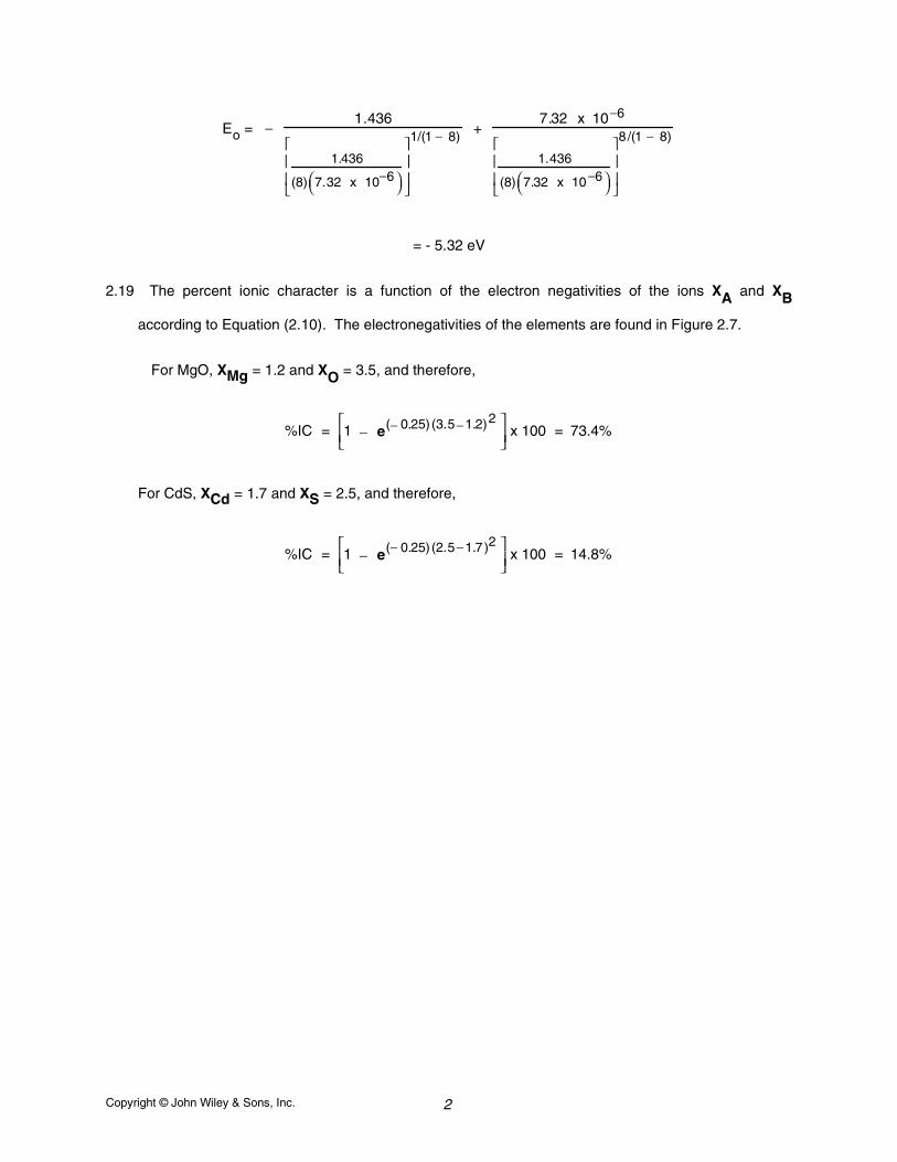
Copyright © John Wiley & Sons, Inc. 2
Eo = − 1.436
1.436
(8) 7.32 x 10⁻⁶
1/(1 − 8) + 7.32 x 10⁻⁶
1.436
(8) 7.32 x 10⁻⁶
8/(1 − 8)
= - 5.32 eV
2.19 The percent ionic character is a function of the electron negativities of the ions XA and XB
according to Equation (2.10). The electronegativities of the elements are found in Figure 2.7.
For MgO, XMg = 1.2 and XO = 3.5, and therefore,
%IC = 1 − e(− 0.25) (3.5−1.2)2
x 100 = 73.4%
For CdS, XCd = 1.7 and XS = 2.5, and therefore,
%IC = 1 − e(− 0.25) (2.5−1.7)2
x 100 = 14.8%
Copyright © John Wiley & Sons, Inc. 3
CHAPTER 3
THE STRUCTURE OF CRYSTALLINE SOLIDS
PROBLEM SOLUTIONS
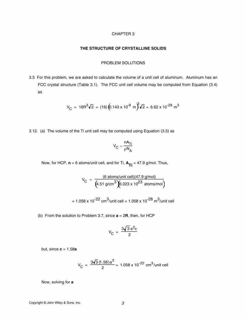
3.3 For this problem, we are asked to calculate the volume of a unit cell of aluminum. Aluminum has an
FCC crystal structure (Table 3.1). The FCC unit cell volume may be computed from Equation (3.4)
as
VC = 16R3 2 = (16) 0.143 x 10⁻⁹ m( )3 2 = 6.62 x 10⁻²⁹ m3
3.12. (a) The volume of the Ti unit cell may be computed using Equation (3.5) as
VC =nATiρNA
Now, for HCP, n = 6 atoms/unit cell, and for Ti, ATi
= 47.9 g/mol. Thus,
VC = (6 atoms/unit cell)(47.9 g/mol)
4.51 g/cm3( )6.023 x 10²³ atoms/mol( )
= 1.058 x 10⁻²² cm3/unit cell = 1.058 x 10⁻²⁸ m3/unit cell
(b) From the solution to Problem 3.7, since a = 2R, then, for HCP
VC = 3 3 a2c
2
but, since c = 1.58a
VC = 3 3 (1.58)a3
2= 1.058 x 10⁻²² cm3/unit cell
Now, solving for a
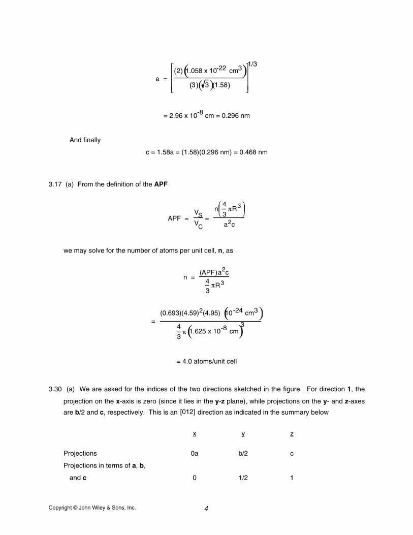
Copyright © John Wiley & Sons, Inc. 4
a = 2( ) 1.058 x 10⁻²² cm3( )
3( ) 3( )1.58( )
1/3
= 2.96 x 10⁻⁸ cm = 0.296 nm
And finally
c = 1.58a = (1.58)(0.296 nm) = 0.468 nm
3.17 (a) From the definition of the APF
APF = VSVC
= n
4
3πR3
a2c
we may solve for the number of atoms per unit cell, n, as
n = (APF)a2c
43
πR3
= (0.693)(4.59)2(4.95) 10-24 cm3( )
4
3π 1.625 x 10⁻⁸ cm( )3
= 4.0 atoms/unit cell
3.30 (a) We are asked for the indices of the two directions sketched in the figure. For direction 1, the
projection on the x-axis is zero (since it lies in the y-z plane), while projections on the y- and z-axes
are b/2 and c, respectively. This is an [012] direction as indicated in the summary below
x y z
Projections 0a b/2 c
Projections in terms of a, b,
and c 0 1/2 1
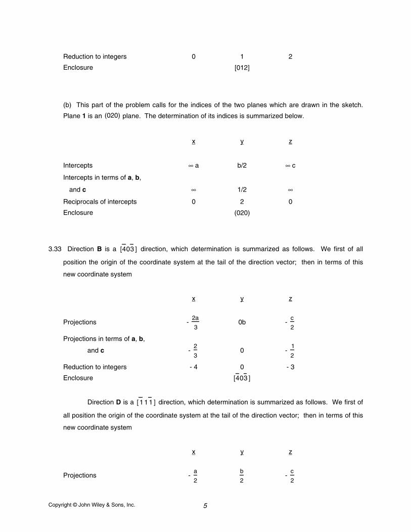
Copyright © John Wiley & Sons, Inc. 5
Reduction to integers 0 1 2
Enclosure [012]
(b) This part of the problem calls for the indices of the two planes which are drawn in the sketch.
Plane 1 is an (020) plane. The determination of its indices is summarized below.
x y z
Intercepts ∞ a b/2 ∞ c
Intercepts in terms of a, b,
and c ∞ 1/2 ∞
Reciprocals of intercepts 0 2 0
Enclosure (020)
3.33 Direction B is a [4 03 ] direction, which determination is summarized as follows. We first of all
position the origin of the coordinate system at the tail of the direction vector; then in terms of this
new coordinate system
x y z
Projections - 2a
30b -
c
2
Projections in terms of a, b,
and c - 2
30 -
1
2
Reduction to integers - 4 0 - 3
Enclosure [4 03 ]
Direction D is a [ 1 1 1 ] direction, which determination is summarized as follows. We first of
all position the origin of the coordinate system at the tail of the direction vector; then in terms of this
new coordinate system
x y z
Projections - a
2
b
2-
c
2
Copyright © John Wiley & Sons, Inc. 6
Projections in terms of a, b,
and c - 1
2
1
2-
1
2
Reduction to integers - 1 1 - 1
Enclosure [1 1 1 ]
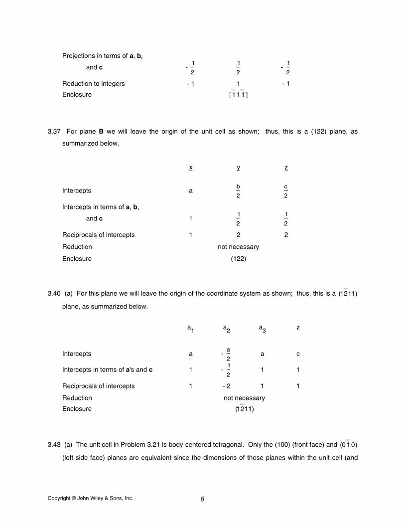
3.37 For plane B we will leave the origin of the unit cell as shown; thus, this is a (122) plane, as
summarized below.
x y z
Intercepts ab
2
c
2
Intercepts in terms of a, b,
and c 11
2
1
2
Reciprocals of intercepts 1 2 2
Reduction not necessary
Enclosure (122)
3.40 (a) For this plane we will leave the origin of the coordinate system as shown; thus, this is a (12 11)
plane, as summarized below.
a1 a2 a3 z
Intercepts a - a
2a c
Intercepts in terms of a's and c 1 - 1
21 1
Reciprocals of intercepts 1 - 2 1 1
Reduction not necessary
Enclosure (12 11)
3.43 (a) The unit cell in Problem 3.21 is body-centered tetragonal. Only the (100) (front face) and (0 1 0)
(left side face) planes are equivalent since the dimensions of these planes within the unit cell (and
Copyright © John Wiley & Sons, Inc. 7
therefore the distances between adjacent atoms) are the same (namely 0.45 nm x 0.35 nm), which
are different than the (001) (top face) plane (namely 0.35 nm x 0.35 nm).
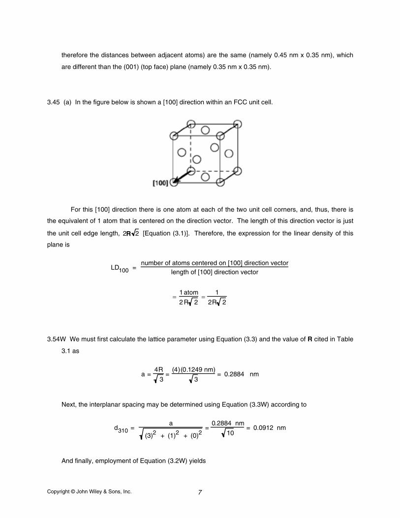
3.45 (a) In the figure below is shown a [100] direction within an FCC unit cell.
For this [100] direction there is one atom at each of the two unit cell corners, and, thus, there is
the equivalent of 1 atom that is centered on the direction vector. The length of this direction vector is just
the unit cell edge length, 2R 2 [Equation (3.1)]. Therefore, the expression for the linear density of this
plane is
LD100 = number of atoms centered on [100] direction vector
length of [100] direction vector
=1 atom
2 R 2=
1
2R 2
3.54W We must first calculate the lattice parameter using Equation (3.3) and the value of R cited in Table
3.1 as
a =4R
3=
(4)(0.1249 nm)
3= 0.2884 nm
Next, the interplanar spacing may be determined using Equation (3.3W) according to
d310 = a
(3)2 + (1)2 + (0)2=
0.2884 nm
10= 0.0912 nm
And finally, employment of Equation (3.2W) yields
Copyright © John Wiley & Sons, Inc. 8
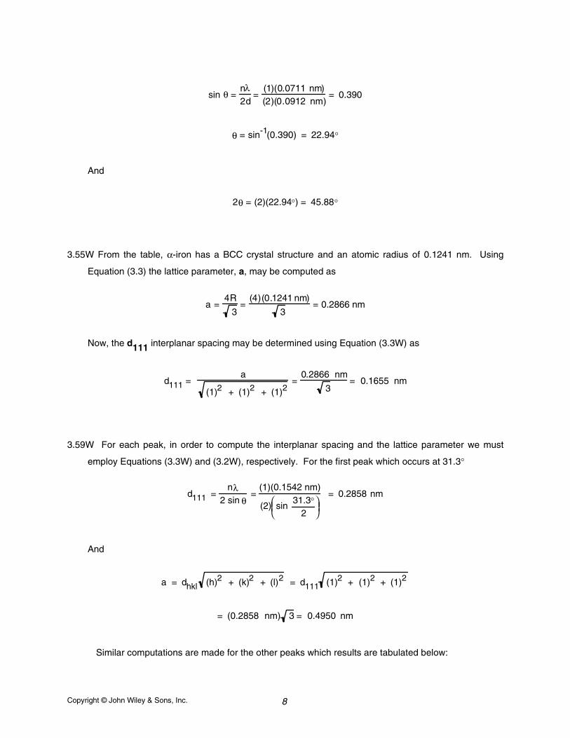
sin θ =nλ2d
=(1)(0.0711 nm)(2)(0.0912 nm)
= 0.390
θ = sin-1(0.390) = 22.94°
And
2θ = (2)(22.94°) = 45.88°
3.55W From the table, α-iron has a BCC crystal structure and an atomic radius of 0.1241 nm. Using
Equation (3.3) the lattice parameter, a, may be computed as
a =4R
3=
(4)(0.1241 nm)
3= 0.2866 nm
Now, the d111 interplanar spacing may be determined using Equation (3.3W) as
d111 = a
(1)2 + (1)2 + (1)2=
0.2866 nm
3= 0.1655 nm
3.59W For each peak, in order to compute the interplanar spacing and the lattice parameter we must
employ Equations (3.3W) and (3.2W), respectively. For the first peak which occurs at 31.3°
d111 =nλ
2 sin θ=
(1)(0.1542 nm)
(2) sin 31.3°
2
= 0.2858 nm
And
a = dhkl (h)2 + (k)2 + (l)2 = d111 (1)2 + (1)2 + (1)2
= (0.2858 nm) 3 = 0.4950 nm
Similar computations are made for the other peaks which results are tabulated below:
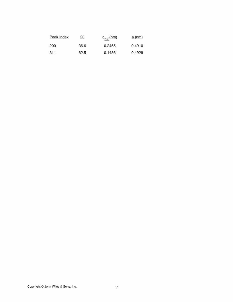
Copyright © John Wiley & Sons, Inc. 9
Peak Index 2θ dhkl(nm) a (nm)
200 36.6 0.2455 0.4910
311 62.5 0.1486 0.4929
Copyright © John Wiley & Sons, Inc. 10
CHAPTER 4
IMPERFECTIONS IN SOLIDS
PROBLEM SOLUTIONS
4.1 In order to compute the fraction of atom sites that are vacant in lead at 600 K, we must employEquation (4.1). As stated in the problem, Q
v = 0.55 eV/atom. Thus,
NVN
= exp −QVkT
= exp −
0.55 eV /atom
8.62 x 10⁻⁵ eV /atom -K( )(600 K)
= 2.41 x 10⁻⁵
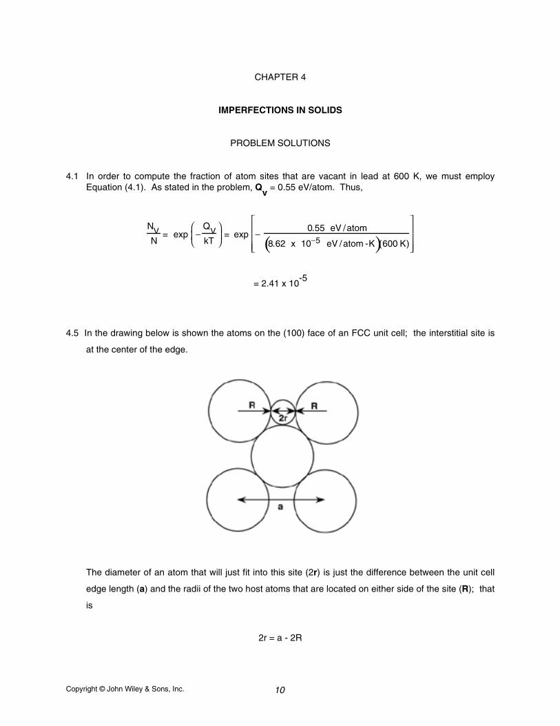
4.5 In the drawing below is shown the atoms on the (100) face of an FCC unit cell; the interstitial site is
at the center of the edge.
The diameter of an atom that will just fit into this site (2r) is just the difference between the unit cell
edge length (a) and the radii of the two host atoms that are located on either side of the site (R); that
is
2r = a - 2R
Copyright © John Wiley & Sons, Inc. 11
However, for FCC a is related to R according to Equation (3.1) as a = 2R 2 ; therefore, solving for
r gives
r = a − 2 R
2=
2R 2 − 2R2
= 0.41R
4.10 The concentration of an element in an alloy, in atom percent, may be computed using Equation
(4.5). With this problem, it first becomes necessary to compute the number of moles of both Cu and
Zn, for which Equation (4.4) is employed. Thus, the number of moles of Cu is just
nmCu
= mCu
'
A Cu =
33 g63.55 g /mol
= 0.519 mol
Likewise, for Zn
nmZn =
47 g65.39 g /mol
= 0.719 mol
Now, use of Equation (4.5) yields
CCu' =
nmCunmCu
+ nmZn
x 100
= 0.519 mol
0.519 mol + 0.719 mol x 100 = 41.9 at%
Also,
CZn' =
0.719 mol0.519 mol + 0.719 mol
x 100 = 58.1 at%
4.14 This problem calls for a determination of the number of atoms per cubic meter for aluminum. In
order to solve this problem, one must employ Equation (4.2),
N = NA ρAl
AAl
Copyright © John Wiley & Sons, Inc. 12
The density of Al (from the table inside of the front cover) is 2.71 g/cm3, while its atomic weight is
26.98 g/mol. Thus,
N = 6.023 x 10²³ atoms/mol( )2.71 g /cm3( )
26.98 g /mol
= 6.05 x 10²² atoms/cm3 = 6.05 x 1028 atoms/m3
4.22 This problem asks us to determine the weight percent of Ge that must be added to Si such that the
resultant alloy will contain 2.43 x10²¹ Ge atoms per cubic centimeter. To solve this problem,
employment of Equation (4.18) is necessary, using the following values:
N1 = NGe = 2.43 x 10²¹ atoms/cm3
ρ1 = ρGe = 5.32 g/cm3
ρ2 = ρSi = 2.33 g/cm3
A1 = AGe = 72.59 g/mol
A2 = ASi = 28.09 g/mol
Thus
CGe = 100
1 + NAρSi
NGeA Ge −
ρSiρGe
= 100
1 + 6.023 x10²³ atoms/ mol( )(2.33 g / cm3)
2.43 x10²¹ atoms / cm3( )(72.59 g /mol) −
2.33 g/ cm3
5.32 g/ cm3
= 11.7 wt%
Copyright © John Wiley & Sons, Inc. 13
4.25 (a) The Burgers vector will point in that direction having the highest linear density. From Section
3.11, the linear density for the [110] direction in FCC is 1/2R, the maximum possible; therefore for
FCC
b = a2
[110]
(b) For Cu which has an FCC crystal structure, R = 0.1278 nm (Table 3.1) and a = 2R 2 =
0.3615 nm [Equation (3.1)]; therefore
b = a2
h2 + k2 + l2
= 0.3615 nm
2(1 )2 + (1 )2 + (0)2 = 0.2556 nm
4.32 (a) This part of problem asks that we compute the number of grains per square inch for an ASTM
grain size of 6 at a magnification of 100x. All we need do is solve for the parameter N in Equation
4.16, inasmuch as n = 6. Thus
N = 2n−1
= 26 −1 = 32 grains/in.2
(b) Now it is necessary to compute the value of N for no magnification. In order to solve this
problem it is necessary to use the following equation:
NMM
100
2= 2n−1
where NM = the number of grains per square inch at magnification M, and n is the ASTM grain size
number. (The above equation makes use of the fact that, while magnification is a length parameter,
area is expressed in terms of units of length squared. As a consequence, the number of grains per
unit area increases with the square of the increase in magnification.) Without any magnification, M
in the above equation is 1, and therefore,
Copyright © John Wiley & Sons, Inc. 14
N11
100
2= 26 −1 = 32
And, solving for N1, N1 = 320,000 grains/in.2.
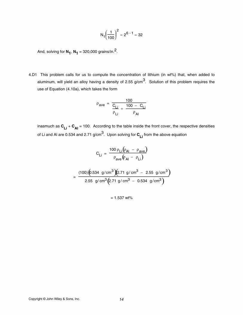
4.D1 This problem calls for us to compute the concentration of lithium (in wt%) that, when added to
aluminum, will yield an alloy having a density of 2.55 g/cm3. Solution of this problem requires the
use of Equation (4.10a), which takes the form
ρave = 100
CLiρ
Li
+ 100 − CLi
ρAl
inasmuch as CLi + CAl = 100. According to the table inside the front cover, the respective densities
of Li and Al are 0.534 and 2.71 g/cm3. Upon solving for CLi from the above equation
CLi = 100 ρLi ρAl − ρave( )
ρave
ρAl − ρ
Li( )
= (100) 0.534 g /cm3( )2.71 g / cm3 − 2.55 g /cm3( )
2.55 g/ cm3 2.71 g / cm3 − 0.534 g /cm3( )
= 1.537 wt%
Copyright © John Wiley & Sons, Inc. 15
CHAPTER 5
DIFFUSION
PROBLEM SOLUTIONS
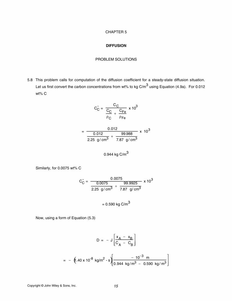
5.8 This problem calls for computation of the diffusion coefficient for a steady-state diffusion situation.
Let us first convert the carbon concentrations from wt% to kg C/m3 using Equation (4.9a). For 0.012
wt% C
CC'' =
CCCCρC
+ CFeρFe
x 103
= 0.012
0.012
2.25 g / cm3 +
99.988
7.87 g / cm3
x 103
0.944 kg C/m3
Similarly, for 0.0075 wt% C
CC'' =
0.00750.0075
2.25 g / cm3 + 99.9925
7.87 g/ cm3
x 103
= 0.590 kg C/m3
Now, using a form of Equation (5.3)
D = − J xA − xBCA − CB
= − 1.40 x 10⁻⁸ kg/m2 - s( ) − 10−3 m
0.944 kg /m3 − 0.590 kg / m3
Copyright © John Wiley & Sons, Inc. 16
= 3.95 x 10⁻¹¹ m2/s
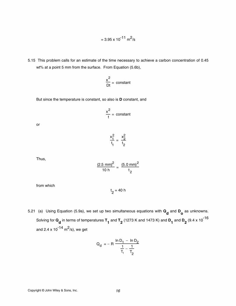
5.15 This problem calls for an estimate of the time necessary to achieve a carbon concentration of 0.45
wt% at a point 5 mm from the surface. From Equation (5.6b),
x2
Dt= constant
But since the temperature is constant, so also is D constant, and
x2
t= constant
or
x12
t1=
x22
t2
Thus,
(2.5 mm)2
10 h=
(5.0 mm)2
t2
from whicht2 = 40 h
5.21 (a) Using Equation (5.9a), we set up two simultaneous equations with Qd
and Do
as unknowns.
Solving for Qd
in terms of temperatures T1 and T
2 (1273
K and 1473
K) and D
1 and D
2 (9.4 x 10
-16
and 2.4 x 10⁻¹⁴ m2/s), we get
Qd = − R ln D1 − ln D2
1
T1
− 1T2
Copyright © John Wiley & Sons, Inc. 17
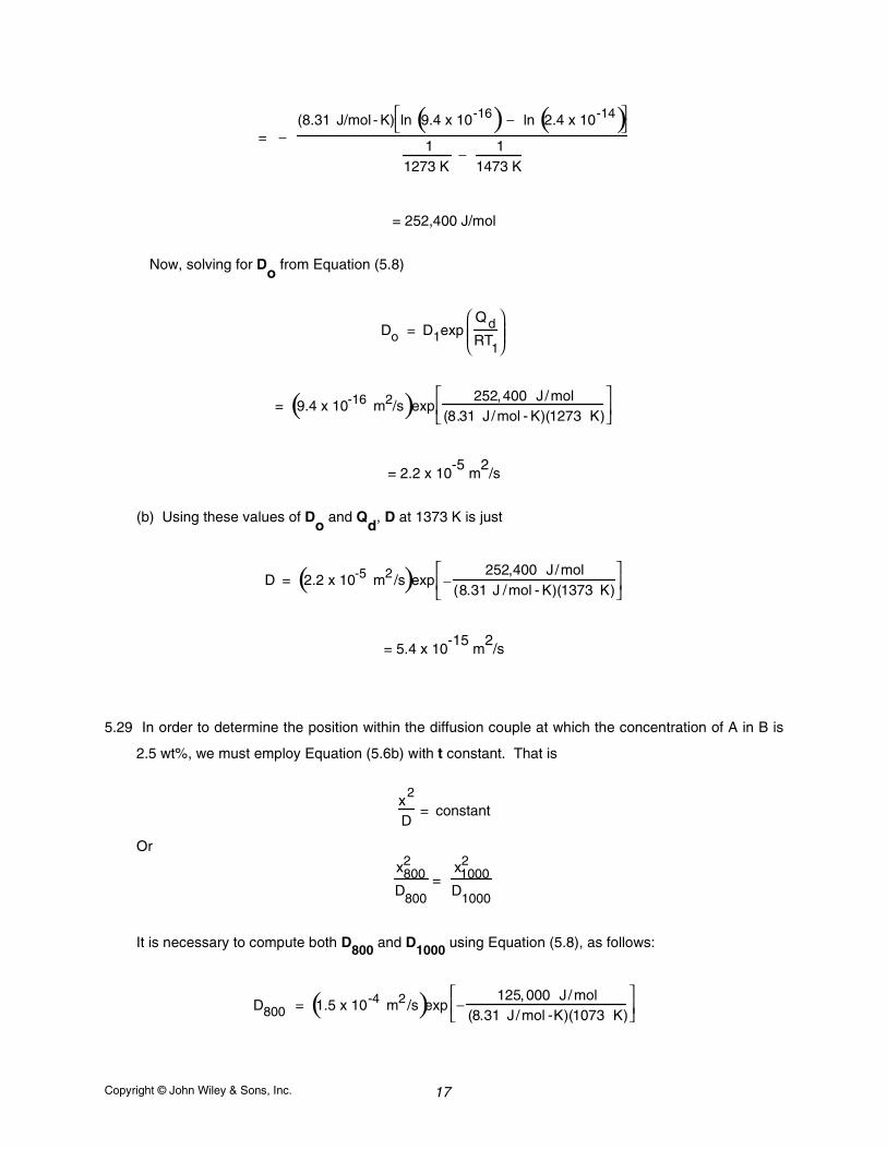
= − (8.31 J/mol - K) ln 9.4 x 10⁻¹⁶( ) − ln 2.4 x 10⁻¹⁴( )
11273 K
− 11473 K
= 252,400 J/mol
Now, solving for Do
from Equation (5.8)
Do = D1expQdRT1
= 9.4 x 10⁻¹⁶ m2/s( )exp252,400 J/mol
(8.31 J/mol - K)(1273 K)
= 2.2 x 10⁻⁵
m2
/s
(b) Using these values of Do
and Qd
, D at 1373 K is just
D = 2.2 x 10⁻⁵ m2/s( )exp −252,400 J/mol
(8.31 J /mol - K)(1373 K)
= 5.4 x 10⁻¹⁵
m2/s
5.29 In order to determine the position within the diffusion couple at which the concentration of A in B is
2.5 wt%, we must employ Equation (5.6b) with t constant. That is
x2
D= constant
Or
x8002
D800=
x10002
D1000
It is necessary to compute both D800 and D1000 using Equation (5.8), as follows:
D800 = 1.5 x 10⁻⁴ m2/s( )exp −125,000 J/mol
(8.31 J/mol -K)(1073 K)
Copyright © John Wiley & Sons, Inc. 18
= 1.22 x 10⁻¹⁰ m2/s
D1000 = 1.5 x 10⁻⁴ m2/s( )exp −125,000 J/mol
(8.31 J/ mol- K)(1273 K)
= 1.11 x 10⁻⁹ m2/s
Now, solving for x1000 yields
x1000 = x800
D1000D800
= (5 mm)1.11 x 10⁻⁹ m2 /s
1.22 x 10⁻¹⁰ m2 /s
= 15.1 mm
Copyright © John Wiley & Sons, Inc. 19
CHAPTER 6
MECHANICAL PROPERTIES OF METALS
PROBLEM SOLUTIONS
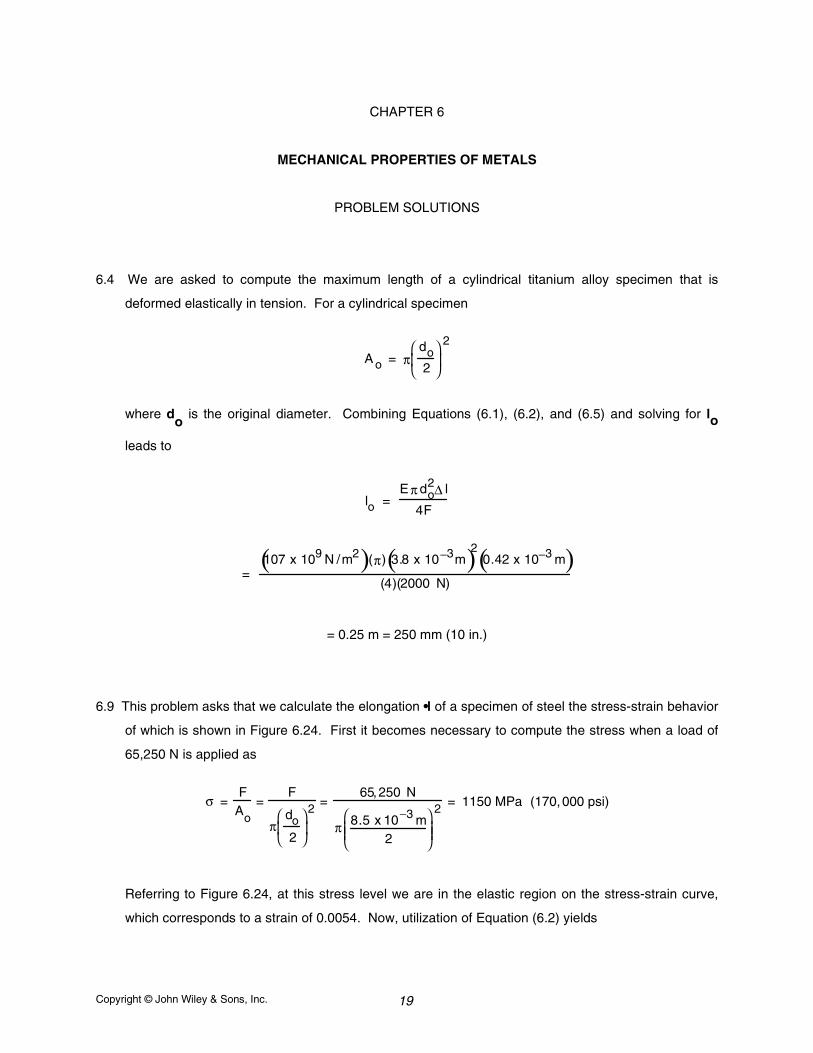
6.4 We are asked to compute the maximum length of a cylindrical titanium alloy specimen that is
deformed elastically in tension. For a cylindrical specimen
A o = πdo2
2
where do
is the original diameter. Combining Equations (6.1), (6.2), and (6.5) and solving for lo
leads to
lo = E π do
2∆ l
4F
= 107 x 109 N /m2( )(π) 3.8 x 10⁻³m( )2 0.42 x 10⁻³ m( )
(4)(2000 N)
= 0.25 m = 250 mm (10 in.)
6.9 This problem asks that we calculate the elongation •l of a specimen of steel the stress-strain behavior
of which is shown in Figure 6.24. First it becomes necessary to compute the stress when a load of
65,250 N is applied as
σ =F
Ao=
F
πdo2
2 =65,250 N
π 8.5 x 10⁻³ m2
2 = 1150 MPa (170,000 psi)
Referring to Figure 6.24, at this stress level we are in the elastic region on the stress-strain curve,
which corresponds to a strain of 0.0054. Now, utilization of Equation (6.2) yields
Copyright © John Wiley & Sons, Inc. 20
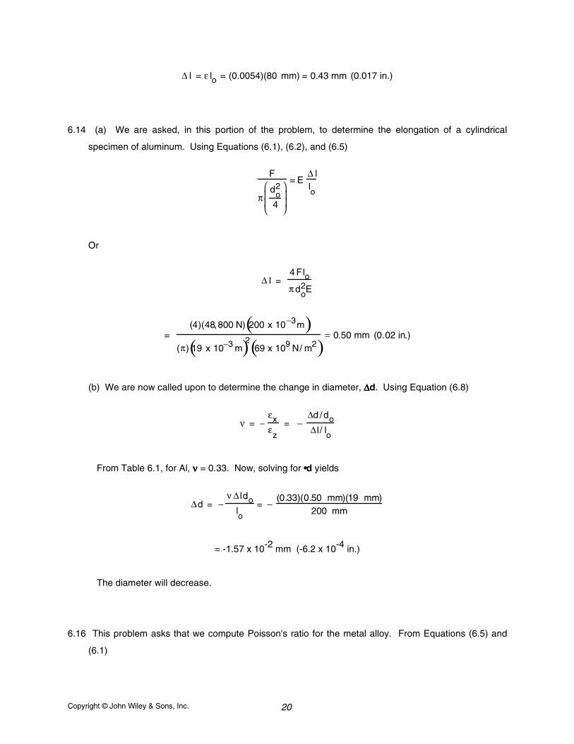
∆ l = ε lo = (0.0054)(80 mm) = 0.43 mm (0.017 in.)
6.14 (a) We are asked, in this portion of the problem, to determine the elongation of a cylindrical
specimen of aluminum. Using Equations (6.1), (6.2), and (6.5)
F
πdo
2
4
= E∆ llo
Or
∆ l = 4 Floπ do
2E
= (4)(48,800 N) 200 x 10−3m( )
(π) 19 x 10−3 m( )2 69 x 109 N/ m2( )= 0.50 mm (0.02 in.)
(b) We are now called upon to determine the change in diameter, ∆∆∆∆d. Using Equation (6.8)
ν = −εxεz
= −∆d /do∆ l / lo
From Table 6.1, for Al, νννν = 0.33. Now, solving for •d yields
∆d = −ν ∆ ldo
lo= −
(0.33)(0.50 mm)(19 mm)200 mm
= -1.57 x 10⁻² mm (-6.2 x 10⁻⁴ in.)
The diameter will decrease.
6.16 This problem asks that we compute Poisson's ratio for the metal alloy. From Equations (6.5) and
(6.1)
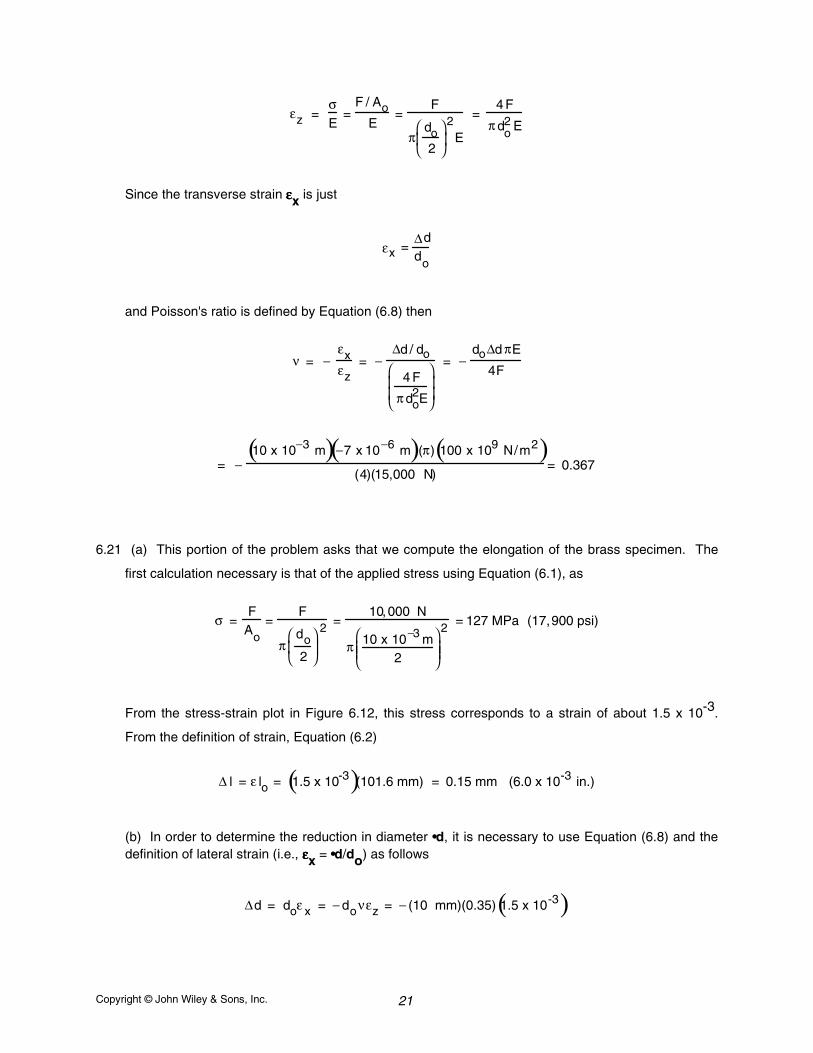
Copyright © John Wiley & Sons, Inc. 21
εz = σE
=F / Ao
E=
F
πdo2
2
E
=4 F
π do2 E
Since the transverse strain εεεεx is just
εx =∆ddo
and Poisson's ratio is defined by Equation (6.8) then
ν = −εxεz
= −∆d / do
4 F
π do2E
= −do∆d πE
4F
= −10 x 10−3 m( )−7 x 10⁻⁶ m( )(π) 100 x 109 N/m2( )
(4)(15,000 N)= 0.367
6.21 (a) This portion of the problem asks that we compute the elongation of the brass specimen. The
first calculation necessary is that of the applied stress using Equation (6.1), as
σ =F
Ao=
F
πdo2
2 =10,000 N
π 10 x 10−3 m2
2 = 127 MPa (17,900 psi)
From the stress-strain plot in Figure 6.12, this stress corresponds to a strain of about 1.5 x 10⁻³.
From the definition of strain, Equation (6.2)
∆ l = ε lo = 1.5 x 10⁻³( )(101.6 mm) = 0.15 mm (6.0 x 10⁻³ in.)
(b) In order to determine the reduction in diameter •d, it is necessary to use Equation (6.8) and thedefinition of lateral strain (i.e., εεεεx = •d/do) as follows
∆d = doε x = − doνεz = − (10 mm)(0.35) 1.5 x 10⁻³( )
Copyright © John Wiley & Sons, Inc. 22
= -5.25 x 10⁻³ mm (-2.05 x 10⁻⁴ in.)
6.27 This problem asks us to determine the deformation characteristics of a steel specimen, the stress-
strain behavior of which is shown in Figure 6.24.
(a) In order to ascertain whether the deformation is elastic or plastic, we must first compute the
stress, then locate it on the stress-strain curve, and, finally, note whether this point is on the elastic
or plastic region. Thus,
σ =F
Ao=
140,000 N
π 10 x 10−3 m2
2 = 1782 MPa (250,000 psi)
The 1782 MPa point is past the linear portion of the curve, and, therefore, the deformation will be
both elastic and plastic.
(b) This portion of the problem asks us to compute the increase in specimen length. From the
stress-strain curve, the strain at 1782 MPa is approximately 0.017. Thus, from Equation (6.2)
∆ l = ε lo = (0.017)(500 mm) = 8.5 mm (0.34 in.)
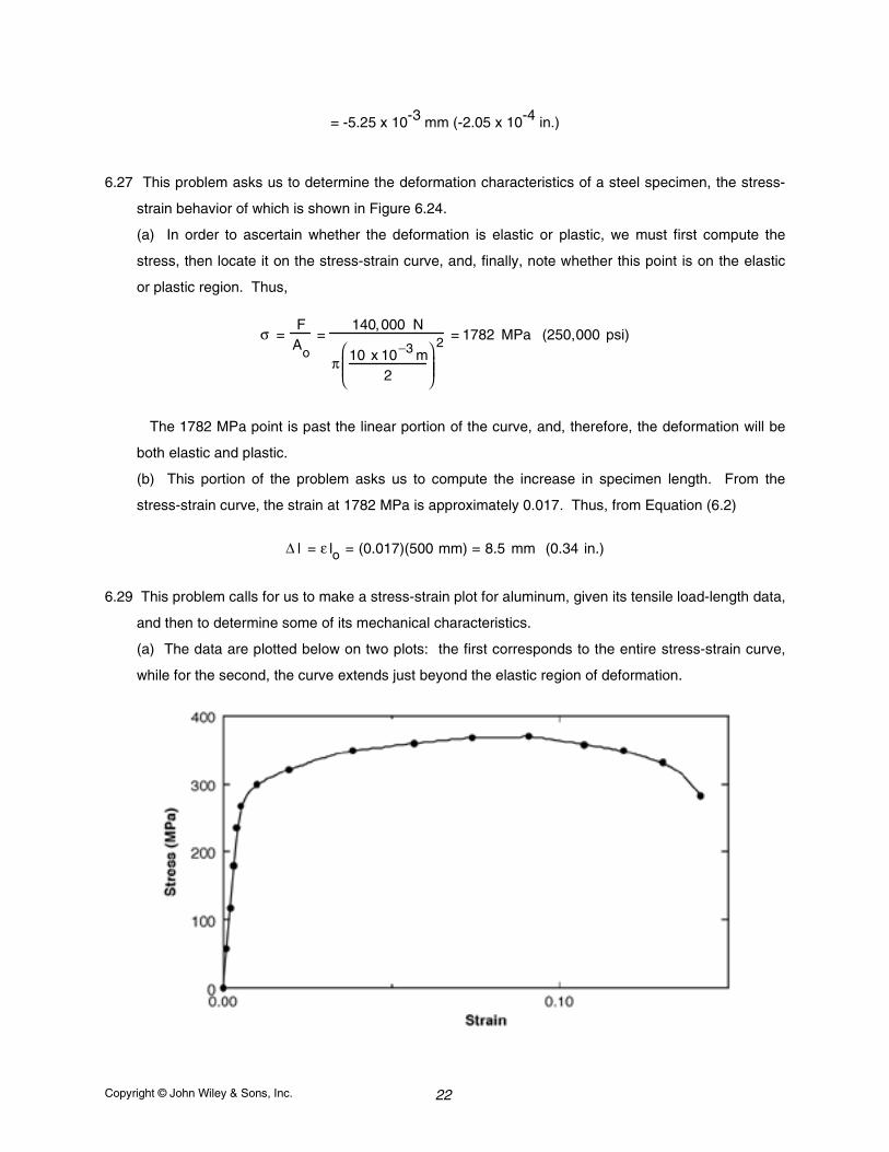
6.29 This problem calls for us to make a stress-strain plot for aluminum, given its tensile load-length data,
and then to determine some of its mechanical characteristics.
(a) The data are plotted below on two plots: the first corresponds to the entire stress-strain curve,
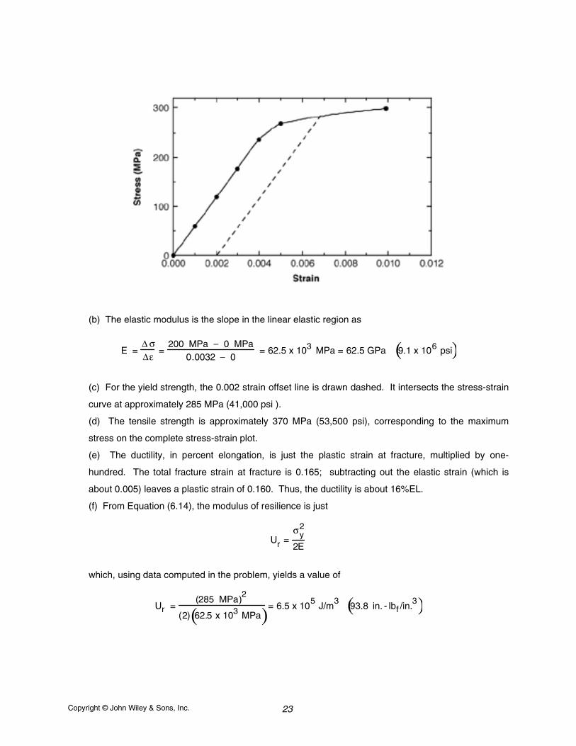
while for the second, the curve extends just beyond the elastic region of deformation.
Copyright © John Wiley & Sons, Inc. 23
(b) The elastic modulus is the slope in the linear elastic region as
E =∆ σ∆ε
=200 MPa − 0 MPa
0.0032 − 0= 62.5 x 10³ MPa = 62.5 GPa 9.1 x 10⁶ psi( )
(c) For the yield strength, the 0.002 strain offset line is drawn dashed. It intersects the stress-strain
curve at approximately 285 MPa (41,000 psi ).
(d) The tensile strength is approximately 370 MPa (53,500 psi), corresponding to the maximum
stress on the complete stress-strain plot.
(e) The ductility, in percent elongation, is just the plastic strain at fracture, multiplied by one-
hundred. The total fracture strain at fracture is 0.165; subtracting out the elastic strain (which is
about 0.005) leaves a plastic strain of 0.160. Thus, the ductility is about 16%EL.
(f) From Equation (6.14), the modulus of resilience is just
Ur =σy
2
2E
which, using data computed in the problem, yields a value of
Ur =(285 MPa)
2
(2) 62.5 x 10³ MPa( )= 6.5 x 10⁵
J/m3 93.8 in. - lbf /in.
3( )
Copyright © John Wiley & Sons, Inc. 24
6.32 This problem asks us to calculate the moduli of resilience for the materials having the stress-strain
behaviors shown in Figures 6.12 and 6.24. According to Equation (6.14), the modulus of resilienceUr is a function of the yield strength and the modulus of elasticity as
Ur =σ
y2
2E
The values for σσσσy and E for the brass in Figure 6.12 are 250 MPa (36,000 psi) and 93.9 GPa (13.6 x
106 psi), respectively. Thus
Ur =(250 MPa)2
(2) 93.9 x 10³ MPa( )= 3.32 x 10⁵ J/m3 47.6 in. - lbf/in.3( )
6.41 For this problem, we are given two values of εεεεT and σσσσT, from which we are asked to calculate the
true stress which produces a true plastic strain of 0.25. After taking logarithms of Equation (6.19),
we may set up two simultaneous equations with two unknowns (the unknowns being K and n), as
log (50,000 psi) = log K + n log (0.10)
log (60,000 psi) = log K + n log (0.20)
From these two expressions,
n =log (50,000) − log (60,000)
log (0.1) − log (0.2)= 0.263
log K = 4.96 or K = 91,623 psi
Thus, for εεεεT = 0.25
σT = K εT( )0.263= (91,623 psi)(0.25)0.263 = 63,700 psi (440 MPa)
6.45 This problem calls for us to utilize the appropriate data from Problem 6.29 in order to determine thevalues of n and K for this material. From Equation (6.38) the slope and intercept of a log σσσσT versus
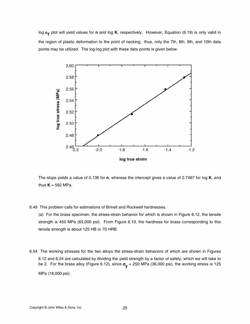
Copyright © John Wiley & Sons, Inc. 25
log εεεεT plot will yield values for n and log K, respectively. However, Equation (6.19) is only valid in
the region of plastic deformation to the point of necking; thus, only the 7th, 8th, 9th, and 10th data
points may be utilized. The log-log plot with these data points is given below.
The slope yields a value of 0.136 for n, whereas the intercept gives a value of 2.7497 for log K, and
thus K = 562 MPa.
6.49 This problem calls for estimations of Brinell and Rockwell hardnesses.
(a) For the brass specimen, the stress-strain behavior for which is shown in Figure 6.12, the tensile
strength is 450 MPa (65,000 psi). From Figure 6.19, the hardness for brass corresponding to this
tensile strength is about 125 HB or 70 HRB.
6.54 The working stresses for the two alloys the stress-strain behaviors of which are shown in Figures
6.12 and 6.24 are calculated by dividing the yield strength by a factor of safety, which we will take tobe 2. For the brass alloy (Figure 6.12), since σσσσy = 250 MPa (36,000 psi), the working stress is 125
MPa (18,000 psi).
Copyright © John Wiley & Sons, Inc. 26
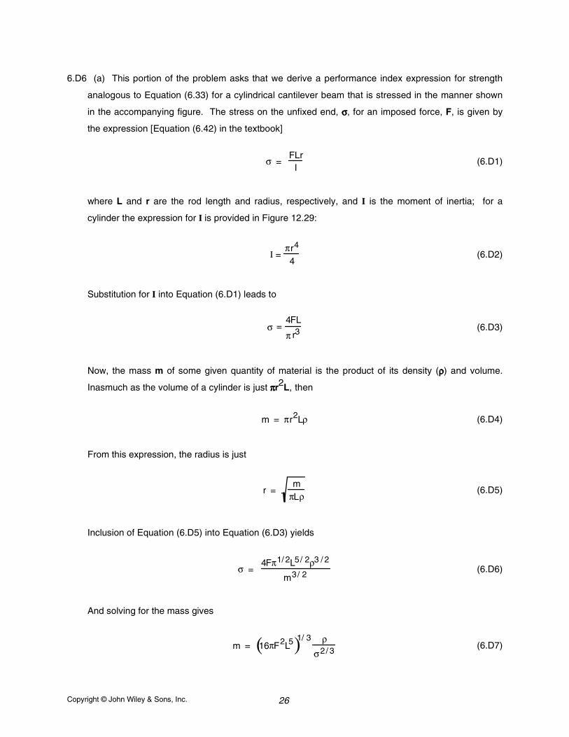
6.D6 (a) This portion of the problem asks that we derive a performance index expression for strength
analogous to Equation (6.33) for a cylindrical cantilever beam that is stressed in the manner shown
in the accompanying figure. The stress on the unfixed end, σσσσ, for an imposed force, F, is given by
the expression [Equation (6.42) in the textbook]
σ =
FLrI
(6.D1)
where L and r are the rod length and radius, respectively, and I is the moment of inertia; for a
cylinder the expression for I is provided in Figure 12.29:
I =
πr4
4(6.D2)
Substitution for I into Equation (6.D1) leads to
σ =4FL
π r3(6.D3)
Now, the mass m of some given quantity of material is the product of its density (ρρρρ) and volume.
Inasmuch as the volume of a cylinder is just ππππr2L, then
m = πr2Lρ (6.D4)
From this expression, the radius is just
r = m
πLρ(6.D5)
Inclusion of Equation (6.D5) into Equation (6.D3) yields
σ = 4Fπ1/ 2L5/ 2ρ3 / 2
m3/ 2(6.D6)
And solving for the mass gives
m = 16πF2L5( )1/ 3 ρσ2/ 3
(6.D7)
Copyright © John Wiley & Sons, Inc. 27
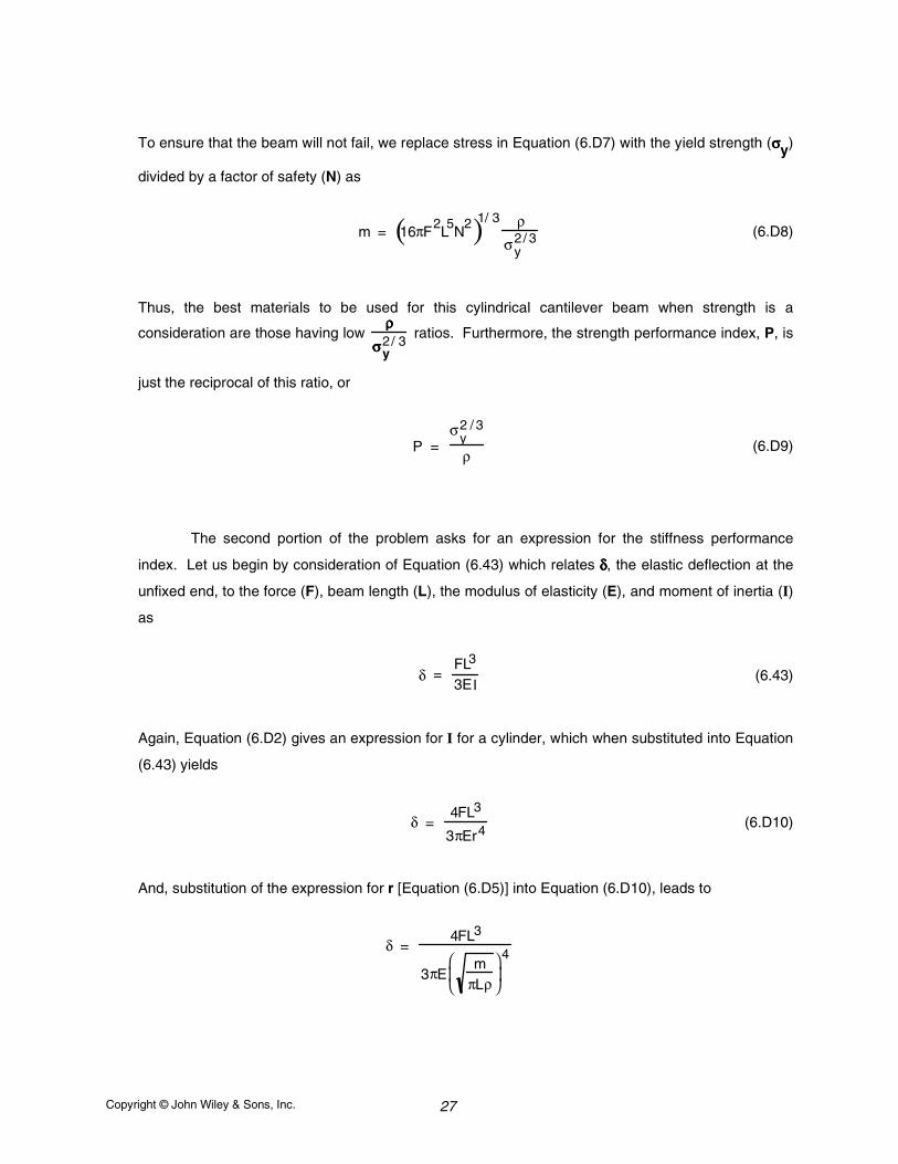
To ensure that the beam will not fail, we replace stress in Equation (6.D7) with the yield strength (σσσσy)
divided by a factor of safety (N) as
m = 16πF2L5N
2( )1/ 3 ρσy
2/ 3 (6.D8)
Thus, the best materials to be used for this cylindrical cantilever beam when strength is a
consideration are those having low ρρρρ
σσσσy2/ 3
ratios. Furthermore, the strength performance index, P, is
just the reciprocal of this ratio, or
P = σ
y2 / 3
ρ(6.D9)
The second portion of the problem asks for an expression for the stiffness performance
index. Let us begin by consideration of Equation (6.43) which relates δδδδ, the elastic deflection at the
unfixed end, to the force (F), beam length (L), the modulus of elasticity (E), and moment of inertia (I)
as
δ =
FL3
3EI(6.43)
Again, Equation (6.D2) gives an expression for I for a cylinder, which when substituted into Equation
(6.43) yields
δ = 4FL3
3πEr4(6.D10)
And, substitution of the expression for r [Equation (6.D5)] into Equation (6.D10), leads to
δ = 4FL3
3πEm
πLρ
4
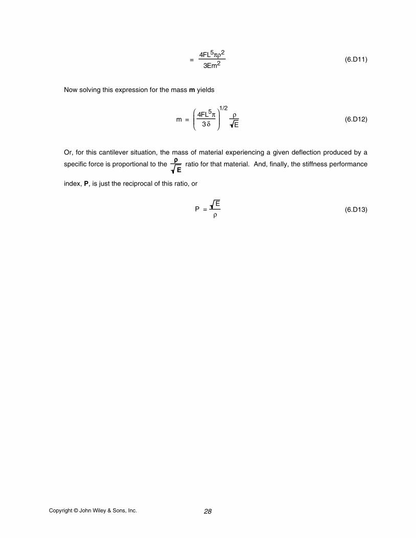
Copyright © John Wiley & Sons, Inc. 28
= 4FL5πρ2
3Em2(6.D11)
Now solving this expression for the mass m yields
m = 4FL5π
3 δ
1/2ρE
(6.D12)
Or, for this cantilever situation, the mass of material experiencing a given deflection produced by a
specific force is proportional to the ρρρρE
ratio for that material. And, finally, the stiffness performance
index, P, is just the reciprocal of this ratio, or
P =E
ρ(6.D13)
Copyright © John Wiley & Sons, Inc. 29
CHAPTER 7
DISLOCATIONS AND STRENGTHENING MECHANISMS
PROBLEM SOLUTIONS
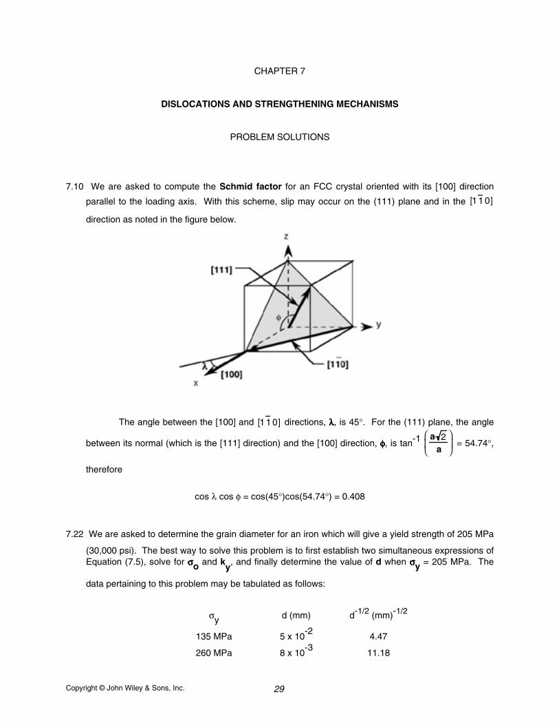
7.10 We are asked to compute the Schmid factor for an FCC crystal oriented with its [100] direction
parallel to the loading axis. With this scheme, slip may occur on the (111) plane and in the [1 1 0]
direction as noted in the figure below.
The angle between the [100] and [1 1 0] directions, λλλλ, is 45°. For the (111) plane, the angle
between its normal (which is the [111] direction) and the [100] direction, φφφφ, is tan-1 a 2
a
= 54.74°,
therefore
cos λ cos φ = cos(45°)cos(54.74°) = 0.408
7.22 We are asked to determine the grain diameter for an iron which will give a yield strength of 205 MPa
(30,000 psi). The best way to solve this problem is to first establish two simultaneous expressions ofEquation (7.5), solve for σσσσo and k
y, and finally determine the value of d when σσσσy = 205 MPa. The
data pertaining to this problem may be tabulated as follows:
σy d (mm) d-1/2 (mm)-1/2
135 MPa 5 x 10⁻²
4.47
260 MPa 8 x 10⁻³
11.18
Copyright © John Wiley & Sons, Inc. 30
The two equations thus become
135 MPa = σo + (4.47) ky
260 MPa = σo + (11.18) ky
Which yield the values, σσσσo = 51.7 MPa and ky = 18.63 MPa(mm)
1/2. At a yield strength of 205 MPa
205 MPa = 51.7 MPa + 18.63 MPa mm( )1/2[ ]d-1/2
or d-1/2
= 8.23 (mm)-1/2
, which gives d = 1.48 x 10⁻²
mm.
7.27 In order for these two cylindrical specimens to have the same deformed hardness, they must be
deformed to the same percent cold work. For the first specimen
%CW =Ao − Ad
Aox 100 =
π ro2 − πrd
2
πro2 x 100
=π (15 mm)2 − π(12 mm)2
π (15 mm)2x 100 = 36%CW
For the second specimen, the deformed radius is computed using the above equation and solving forrd as
rd = ro 1 −%CW100
= (11 mm) 1 −36%CW
100= 8.80 mm
7.29 This problem calls for us to calculate the precold-worked radius of a cylindrical specimen of copper
that has a cold-worked ductility of 25%EL. From Figure 7.17(c), copper that has a ductility of 25%EL
will have experienced a deformation of about 11%CW. For a cylindrical specimen, Equation (7.6)
becomes
Copyright © John Wiley & Sons, Inc. 31
%CW =πr o
2 − πr d2
π ro2
x 100
Since rd
= 10 mm (0.40 in.), solving for ro
yields
ro =rd
1 −%CW
100
=10 mm
1 −11.0
100
= 10.6 mm (0.424 in.)
7.37 In this problem, we are asked for the length of time required for the average grain size of a brass
material to increase a specified amount using Figure 7.23.
(a) At 500°C, the time necessary for the average grain diameter to increase from 0.01 to 0.1 mm is
approximately 3500 min.
7.D1 This problem calls for us to determine whether or not it is possible to cold work steel so as to give a
minimum Brinell hardness of 240 and a ductility of at least 15%EL. According to Figure 6.19, a
Brinell hardness of 240 corresponds to a tensile strength of 800 MPa (116,000 psi). Furthermore,
from Figure 7.17(b), in order to achieve a tensile strength of 800 MPa, deformation of at least
13%CW is necessary. Finally, if we cold work the steel to 13%CW, then the ductility is 15%EL from
Figure 7.17(c). Therefore, it is possible to meet both of these criteria by plastically deforming the
steel.
7.D6 Let us first calculate the percent cold work and attendant yield strength and ductility if the drawing is
carried out without interruption. From Equation (7.6)
%CW =
πdo2
2
− πdd2
2
πdo2
2 x 100
Copyright © John Wiley & Sons, Inc. 32
=π
10.2 mm
2
2− π
7.6 mm
2
2
π10.2 mm
2
2 x 100 = 44.5%CW
At 44.5%CW, the brass will have a yield strength on the order of 420 MPa (61,000 psi), Figure
7.17(a), which is adequate; however, the ductility will be about 5%EL, Figure 7.17(c), which is
insufficient.
Instead of performing the drawing in a single operation, let us initially draw some fraction of
the total deformation, then anneal to recrystallize, and, finally, cold work the material a second time in
order to achieve the final diameter, yield strength, and ductility.
Reference to Figure 7.17(a) indicates that 26%CW is necessary to give a yield strength of
380 MPa. Similarly, a maximum of 27.5%CW is possible for 15%EL [Figure 7.17(c)]. The average of
these two values is 26.8%CW, which we will use in the calculations. If the final diameter after the first
drawing is do' , then
26.8%CW =
πdo
'
2
2
− π7.6 mm
2
2
πdo
'
2
2 x 100
And, solving for do' yields do
' = 9.4 mm (0.37 in.).
Copyright © John Wiley & Sons, Inc. 33
CHAPTER 8
FAILURE
PROBLEM SOLUTIONS
8.6 We may determine the critical stress required for the propagation of an internal crack in aluminum
oxide using Equation (8.3); taking the value of 393 GPa (Table 12.5) as the modulus of elasticity, we
get
σc =2Eγ s
πa
=(2) 393 x 109 N/m2( )(0.90 N/m)
(π)4 x 10⁻⁴ m
2
= 33.6 x10⁶ N/m2 = 33.6 MPa
8.8W This problem calls for us to calculate the normal σσσσx and σσσσy stresses in front on a surface crack of
length 2.0 mm at various positions when a tensile stress of 100 MPa is applied. Substitution for K =
σσσσ πa into Equations (8.9aW) and (8.9bW) leads to
σx = σ fx(θ)a2r
σy = σ fy(θ)a2r
where fx(θθθθ) and fy(θθθθ) are defined in the accompanying footnote 2. For θθθθ = 0°, fx(θθθθ) = 1.0 and fy(θθθθ) =
1.0, whereas for θθθθ = 45°, fx(θθθθ) = 0.60 and fy(θθθθ) = 1.25.
(a) For r = 0.1 mm and θθθθ = 0°,
σx = σy = σ(1.0)a2r
= (100 MPa)2.0 mm
(2)(0.1 mm)= 316 MPa (45,800 psi)
Copyright © John Wiley & Sons, Inc. 34
(d) For r = 0.5 mm and θθθθ = 45°,
σx = σ(0.6)a2r
= (100 MPa)(0.6)2.0 mm
(2)(0.5 mm)= 84.8 MPa (12,300 psi)
σy = σ(1.25)a2 r
= (100 MPa)(1.25)2.0 mm
(2)(0.5 mm)= 177 MPa (25,600 psi)
8.10W (a) In this portion of the problem it is necessary to compute the stress at point P when the applied
stress is 140 MPa (20,000 psi). In order to determine the stress concentration it is necessary to
consult Figure 8.2cW. From the geometry of the specimen, w/h = (40 mm)/(20 mm) = 2.0;
furthermore, the r/h ratio is (4 mm)/(20 mm) = 0.20. Using the w/h = 2.0 curve in Figure 8.2cW, the
Kt value at r/h = 0.20 is 1.8. And since Kt =σσσσmσσσσ
o, then
σm = Ktσo = (1.8)(140 MPa) = 252 MPa (36,000 psi)
8.13W This problem calls for us to determine the value of B, the minimum component thickness for which
the condition of plane strain is valid using Equation (8.14W), for the metal alloys listed in Table 8.1.
For the 2024-T3 aluminum alloy
B = 2.5 KIcσ
y
2
= (2.5)44 MPa m
345 MPa
2
= 0.0406 m = 40.6 mm (1.60 in.)
For the 4340 alloy steel tempered at 260°C
B = (2.5)50 MPa m
1640 MPa
2
= 0.0023 m = 2.3 mm (0.09 in.)
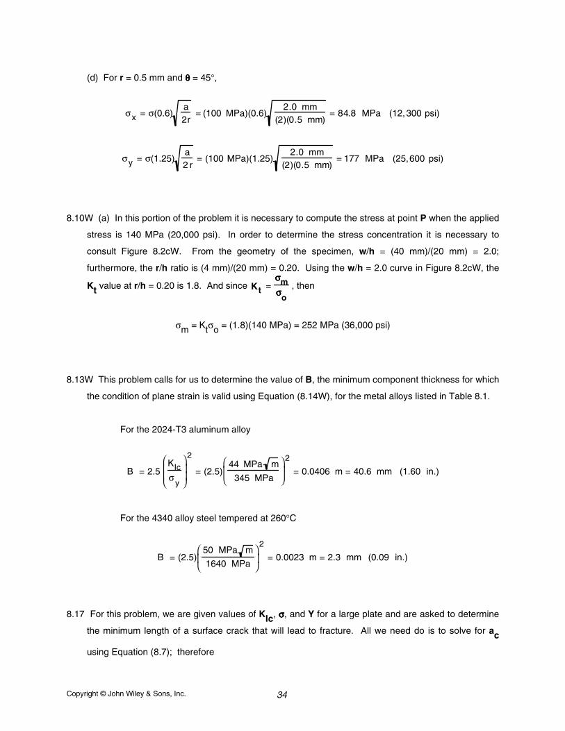
8.17 For this problem, we are given values of KIc, σσσσ, and Y for a large plate and are asked to determine
the minimum length of a surface crack that will lead to fracture. All we need do is to solve for ac
using Equation (8.7); therefore
Copyright © John Wiley & Sons, Inc. 35
ac =1π
KIcYσ
2
=1π
82.4 MPa m
(1)(345 MPa)
2
= 0.0182 m = 18.2 mm (0.72 in.)
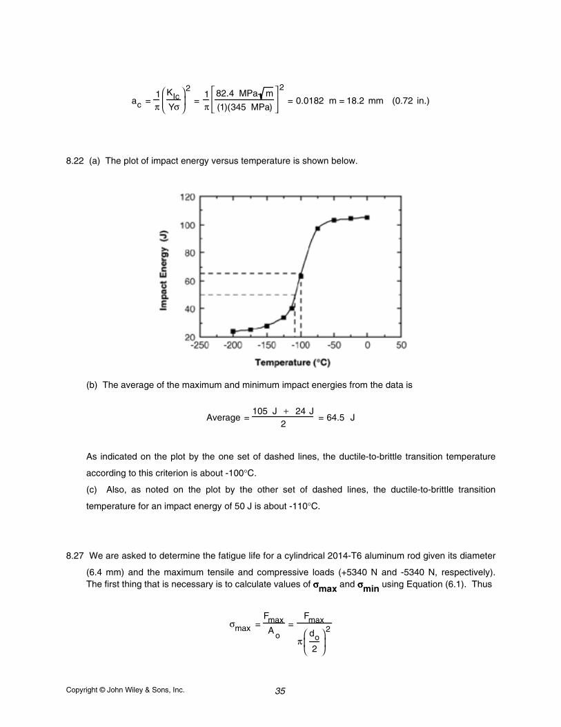
8.22 (a) The plot of impact energy versus temperature is shown below.
(b) The average of the maximum and minimum impact energies from the data is
Average =105 J + 24 J
2= 64.5 J
As indicated on the plot by the one set of dashed lines, the ductile-to-brittle transition temperature
according to this criterion is about -100°C.
(c) Also, as noted on the plot by the other set of dashed lines, the ductile-to-brittle transition
temperature for an impact energy of 50 J is about -110°C.
8.27 We are asked to determine the fatigue life for a cylindrical 2014-T6 aluminum rod given its diameter
(6.4 mm) and the maximum tensile and compressive loads (+5340 N and -5340 N, respectively).The first thing that is necessary is to calculate values of σσσσmax and σσσσmin using Equation (6.1). Thus
σmax =FmaxA o
=Fmax
πdo2
2
Copyright © John Wiley & Sons, Inc. 36
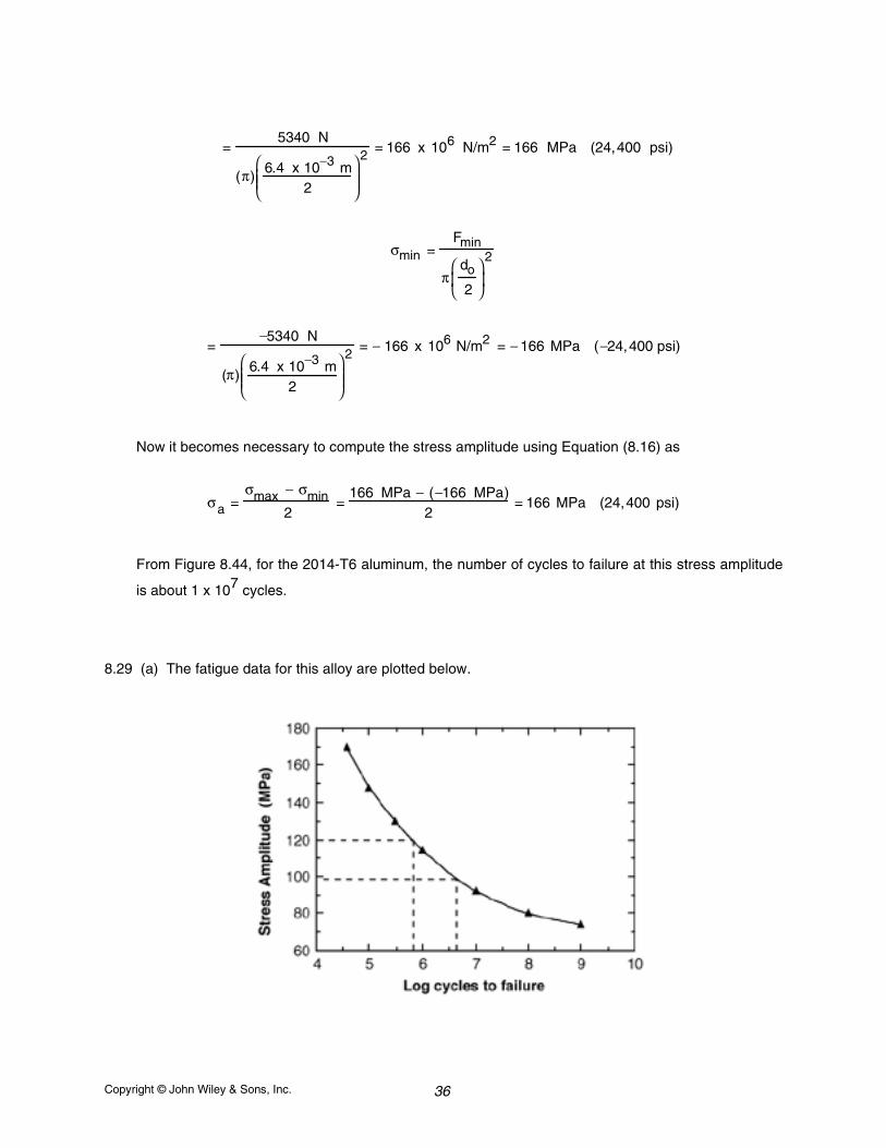
=5340 N
(π)6.4 x 10⁻³ m
2
2 = 166 x 106 N/m2 = 166 MPa (24,400 psi)
σmin =Fmin
πdo
2
2
=−5340 N
(π)6.4 x 10⁻³ m
2
2 = − 166 x 106 N/m2 = − 166 MPa (−24,400 psi)
Now it becomes necessary to compute the stress amplitude using Equation (8.16) as
σa =σmax − σmin
2=
166 MPa − (−166 MPa)2
= 166 MPa (24,400 psi)
From Figure 8.44, for the 2014-T6 aluminum, the number of cycles to failure at this stress amplitude
is about 1 x 10⁷ cycles.
8.29 (a) The fatigue data for this alloy are plotted below.
Copyright © John Wiley & Sons, Inc. 37
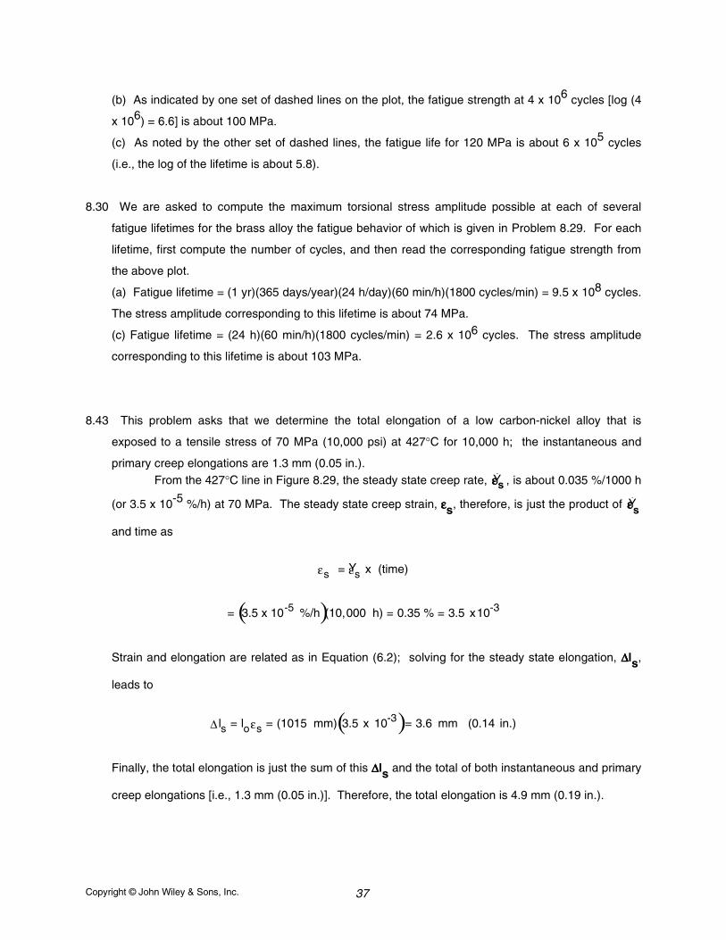
(b) As indicated by one set of dashed lines on the plot, the fatigue strength at 4 x 10⁶ cycles [log (4
x 106) = 6.6] is about 100 MPa.
(c) As noted by the other set of dashed lines, the fatigue life for 120 MPa is about 6 x 10⁵ cycles
(i.e., the log of the lifetime is about 5.8).
8.30 We are asked to compute the maximum torsional stress amplitude possible at each of several
fatigue lifetimes for the brass alloy the fatigue behavior of which is given in Problem 8.29. For each
lifetime, first compute the number of cycles, and then read the corresponding fatigue strength from
the above plot.
(a) Fatigue lifetime = (1 yr)(365 days/year)(24 h/day)(60 min/h)(1800 cycles/min) = 9.5 x 10⁸ cycles.
The stress amplitude corresponding to this lifetime is about 74 MPa.
(c) Fatigue lifetime = (24 h)(60 min/h)(1800 cycles/min) = 2.6 x 10⁶ cycles. The stress amplitude
corresponding to this lifetime is about 103 MPa.
8.43 This problem asks that we determine the total elongation of a low carbon-nickel alloy that is
exposed to a tensile stress of 70 MPa (10,000 psi) at 427°C for 10,000 h; the instantaneous and
primary creep elongations are 1.3 mm (0.05 in.).From the 427°C line in Figure 8.29, the steady state creep rate, Ý ε ε ε ε s , is about 0.035 %/1000 h
(or 3.5 x 10⁻⁵ %/h) at 70 MPa. The steady state creep strain, εεεεs, therefore, is just the product of Ý ε ε ε ε s
and time as
εs = Ý ε s x (time)
= 3.5 x 10⁻⁵ %/h( )(10,000 h) = 0.35 % = 3.5 x10⁻³
Strain and elongation are related as in Equation (6.2); solving for the steady state elongation, ∆∆∆∆ls,
leads to
∆ ls = loεs = (1015 mm) 3.5 x 10⁻³( )= 3.6 mm (0.14 in.)
Finally, the total elongation is just the sum of this ∆∆∆∆ls and the total of both instantaneous and primary
creep elongations [i.e., 1.3 mm (0.05 in.)]. Therefore, the total elongation is 4.9 mm (0.19 in.).
Copyright © John Wiley & Sons, Inc. 38
8.47 The slope of the line from a log Ý ε ε ε ε s versus log σσσσ plot yields the value of n in Equation (8.19); that is
n =∆ log Ý ε s∆ log σ
We are asked to determine the values of n for the creep data at the three temperatures in Figure8.29. This is accomplished by taking ratios of the differences between two log Ý ε ε ε ε s and log σσσσ values.
Thus for 427°C
n =∆ log Ý ε s∆ log σ
=log 10−1( ) − log 10−2( )
log (85 MPa) − log (55 MPa)= 5.3
8.50 This problem gives Ý ε ε ε ε s values at two different temperatures and 140 MPa (20,000 psi), and the
stress exponent n = 8.5, and asks that we determine the steady-state creep rate at a stress of 83
MPa (12,000 psi) and 1300 K.
Taking the natural logarithm of Equation (8.20) yields
ln Ý ε s = ln K2 + n ln σ −QcRT
With the given data there are two unknowns in this equation--namely K2 and Qc. Using the data
provided in the problem we can set up two independent equations as follows:
ln 6.6 x 10⁻⁴ (h)−1[ ]= ln K2 + (8.5) ln (140 MPa) −Qc
(8.31 J /mol - K)(1090 K)
ln 8.8 x 10⁻² (h)−1[ ]= ln K2 + (8.5) ln (140 MPa) −Qc
(8.31 J /mol - K)(1200 K)
Now, solving simultaneously for K2 and Qc leads to K2 = 57.5 (h)-1 and Qc = 483,500 J/mol. Thus,
it is now possible to solve for Ý ε ε ε ε s at 83 MPa and 1300 K using Equation (8.20) as
Ý ε s = K 2σnexp −
QcRT
Copyright © John Wiley & Sons, Inc. 39
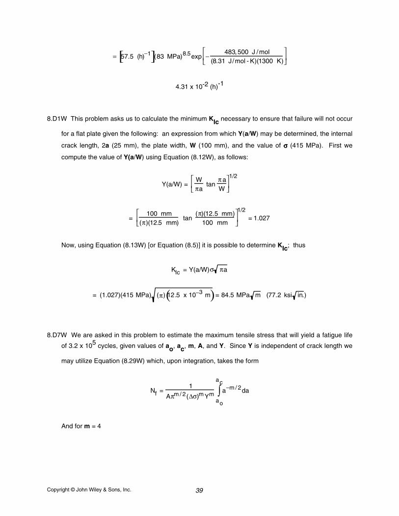
= 57.5 (h)−1[ ](83 MPa)8.5exp −483,500 J /mol
(8.31 J/mol - K)(1300 K)
4.31 x 10⁻² (h)-1
8.D1W This problem asks us to calculate the minimum KIc necessary to ensure that failure will not occur
for a flat plate given the following: an expression from which Y(a/W) may be determined, the internal
crack length, 2a (25 mm), the plate width, W (100 mm), and the value of σσσσ (415 MPa). First we
compute the value of Y(a/W) using Equation (8.12W), as follows:
Y(a/W) =Wπa
tanπ aW
1/2
= 100 mm
(π)(12.5 mm) tan
(π)(12.5 mm)100 mm
1/2
= 1.027
Now, using Equation (8.13W) [or Equation (8.5)] it is possible to determine KIc; thus
KIc = Y(a/W)σ πa
= (1.027)(415 MPa) (π) 12.5 x 10⁻³ m( )= 84.5 MPa m (77.2 ksi in.)
8.D7W We are asked in this problem to estimate the maximum tensile stress that will yield a fatigue life
of 3.2 x 10⁵ cycles, given values of ao, ac, m, A, and Y. Since Y is independent of crack length we
may utilize Equation (8.29W) which, upon integration, takes the form
Nf =1
Aπm / 2(∆σ)m Ym a−m / 2
ao
ac
∫ da
And for m = 4
Copyright © John Wiley & Sons, Inc. 40
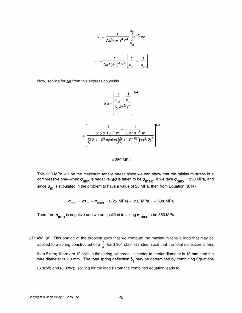
Nf =1
Aπ2(∆σ)4Y4 a −2
ao
ac
∫ da
= −1
Aπ2(∆σ )4Y41
ac
−1
ao
Now, solving for ∆σ∆σ∆σ∆σ from this expression yields
∆σ =
1
ao−
1
ac
Nf Aπ2Y4
1/4
=
1
2.5 x 10⁻⁴ m− 1
5 x 10⁻³ m
3.2 x 10⁵ cycles( )5 x 10⁻¹⁵( )(π)2(2)4
1/4
= 350 MPa
This 350 MPa will be the maximum tensile stress since we can show that the minimum stress is acompressive one--when σσσσmin is negative, ∆σ∆σ∆σ∆σ is taken to be σσσσmax. If we take σσσσmax = 350 MPa, and
since σσσσm is stipulated in the problem to have a value of 25 MPa, then from Equation (8.14)
σmin = 2σm − σmax = 2(25 MPa) − 350 MPa = − 300 MPa
Therefore σσσσmin is negative and we are justified in taking σσσσmax to be 350 MPa.
8.D14W (a) This portion of the problem asks that we compute the maximum tensile load that may be
applied to a spring constructed of a 14
hard 304 stainless steel such that the total deflection is less
than 5 mm; there are 10 coils in the spring, whereas, its center-to-center diameter is 15 mm, and thewire diameter is 2.0 mm. The total spring deflection δδδδs may be determined by combining Equations
(8.32W) and (8.33W); solving for the load F from the combined equation leads to
Copyright © John Wiley & Sons, Inc. 41
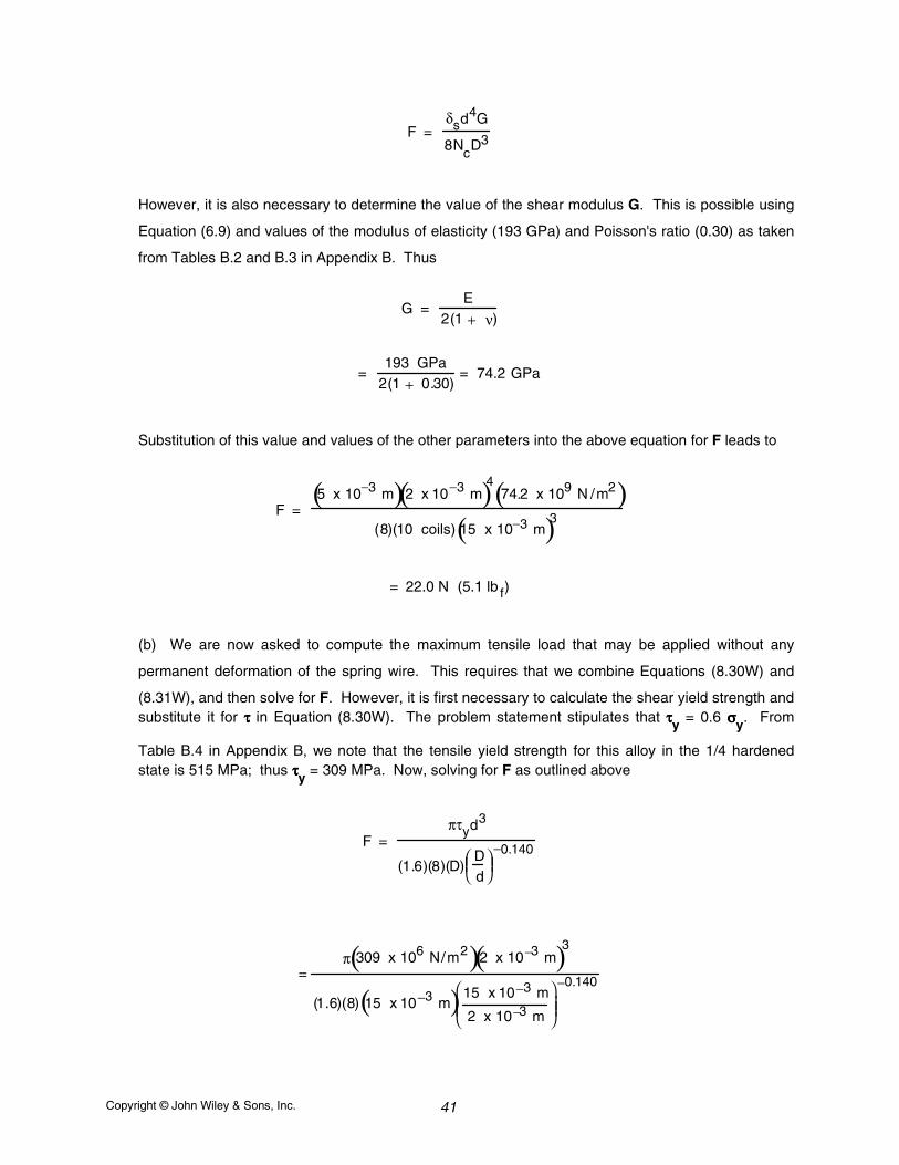
F = δsd4G
8NcD3
However, it is also necessary to determine the value of the shear modulus G. This is possible using
Equation (6.9) and values of the modulus of elasticity (193 GPa) and Poisson's ratio (0.30) as taken
from Tables B.2 and B.3 in Appendix B. Thus
G = E
2(1 + ν)
= 193 GPa
2(1 + 0.30)= 74.2 GPa
Substitution of this value and values of the other parameters into the above equation for F leads to
F = 5 x 10⁻³ m( )2 x 10⁻³ m( )4 74.2 x 10⁹ N /m2( )
(8)(10 coils) 15 x 10−3 m( )3
= 22.0 N (5.1 lb f)
(b) We are now asked to compute the maximum tensile load that may be applied without any
permanent deformation of the spring wire. This requires that we combine Equations (8.30W) and
(8.31W), and then solve for F. However, it is first necessary to calculate the shear yield strength andsubstitute it for ττττ in Equation (8.30W). The problem statement stipulates that ττττy = 0.6 σσσσy. From
Table B.4 in Appendix B, we note that the tensile yield strength for this alloy in the 1/4 hardenedstate is 515 MPa; thus ττττy = 309 MPa. Now, solving for F as outlined above
F = πτyd3
(1.6)(8)(D)Dd
−0.140
=π 309 x 106 N/m2( )2 x 10⁻³ m( )3
(1.6)(8) 15 x 10−3 m( ) 15 x 10−3 m
2 x 10⁻³ m
−0.140
Copyright © John Wiley & Sons, Inc. 42
= 53.6 N (12.5 lb f)
8.D21W We are asked in this problem to calculate the stress levels at which the rupture lifetime will be 1
year and 15 years when an 18-8 Mo stainless steel component is subjected to a temperature of
650°C (923 K). It first becomes necessary to calculate the value of the Larson-Miller parameter for
each time. The values of tr corresponding to 1 and 15 years are 8.76 x 10³ h and 1.31 x 10⁵ h,
respectively. Hence, for a lifetime of 1 year
T 20 + log tr( )= 923 20 + log 8.76 x 10³( )
= 22.10 x 10³
Using the curve shown in Figure 8.45, the stress value corresponding to the one-year lifetime is
approximately 110 MPa (16,000 psi).
Copyright © John Wiley & Sons, Inc. 43
CHAPTER 9
PHASE DIAGRAMS
PROBLEM SOLUTIONS
9.5 This problem asks that we cite the phase or phases present for several alloys at specified
temperatures.
(a) For an alloy composed of 15 wt% Sn-85 wt% Pb and at 100°C, from Figure 9.7, αααα and ββββ phases
are present, andCα = 5 wt% Sn-95 wt% Pb
Cβ = 98 wt% Sn-2 wt% Pb
(c) For an alloy composed of 85 wt% Ag-15 wt% Cu and at 800°C, from Figure 9.6, ββββ and liquid
phases are present, and
Cβ = 92 wt% Ag-8 wt% Cu
CL = 77 wt% Ag-23 wt% Cu
9.7 This problem asks that we determine the phase mass fractions for the alloys and temperatures in
Problem 9.5.
(a)
Wα =Cβ − Co
Cβ − Cα=
98 − 1598 − 5
= 0.89
Wβ =Co − CαCβ − C
α=
15 − 598 − 5
= 0.11
(c)
Wβ =Co − CLCβ − CL
=85 − 7792 − 77
= 0.53
Copyright © John Wiley & Sons, Inc. 44
WL =Cβ − Co
Cβ − CL=
92 − 8592 − 77
= 0.47
9.9 This problem asks that we determine the phase volume fractions for the alloys and temperatures in
Problems 9.5a, b, and d. This is accomplished by using the technique illustrated in Example
Problem 9.3, and the results of Problems 9.5 and 9.7.
(a) This is a Sn-Pb alloy at 100°C, wherein
Cα = 5 wt% Sn-95 wt% Pb
Cβ = 98 wt% Sn-2 wt% Pb
Wα = 0.89
Wβ = 0.11
ρSn = 7.29 g/cm3
ρPb = 11.27 g/cm3
Using these data it is first necessary to compute the densities of the αααα and ββββ phases using Equation
(4.10a). Thus
ρα =100
CSn(α)
ρSn+
CPb(α)
ρPb
=100
5
7.29 g / cm3+
95
11.27 g / cm3
= 10.97 g/cm3
ρβ =100
CSn(β)
ρSn+
CPb(β)
ρPb
=100
98
7.29 g / cm3+ 2
11.27 g / cm3
= 7.34 g/cm3
Copyright © John Wiley & Sons, Inc. 45
Now we may determine the Vαααα and Vββββ values using Equation 9.6. Thus,
Vα =
Wαρα
Wαρα
+Wβρβ
=
0.89
10.97 g/ cm3
0.89
10.97 g /cm3+ 0.11
7.34 g / cm3
= 0.84
Vβ =
Wβρβ
Wαρα
+Wβρβ
=
0.11
7.34 g / cm3
0.89
10.97 g /cm3+ 0.11
7.34 g / cm3
= 0.16
9.12 (a) We are asked to determine how much sugar will dissolve in 1000 g of water at 80°C. From the
solubility limit curve in Figure 9.1, at 80°C the maximum concentration of sugar in the syrup is about
74 wt%. It is now possible to calculate the mass of sugar using Equation (4.3) as
Csugar(wt%) =msugar
msugar+ mwater
× 100
74 wt% =msugar
msugar+ 1000 g
× 100
Solving for msugar yields msugar = 2846 g
(b) Again using this same plot, at 20°C the solubility limit (or the concentration of the saturated
solution) is about 64 wt% sugar.
Copyright © John Wiley & Sons, Inc. 46
(c) The mass of sugar in this saturated solution at 20°C (msugar') may also be calculated using
Equation (4.3) as follows:
64 wt% =msugar '
msugar' + 1000 g× 100
which yields a value for msugar' of 1778 g. Subtracting the latter from the former of these sugar
concentrations yields the amount of sugar that precipitated out of the solution upon coolingmsugar"; that is
msugar" = msugar - msugar' = 2846 g - 1778 g = 1068 g
9.21 Upon cooling a 50 wt% Ni-50 wt% Cu alloy from 1400°C and utilizing Figure 9.2a:
(a) The first solid phase forms at the temperature at which a vertical line at this composition
intersects the L-(αααα + L) phase boundary--i.e., at about 1320°C;
(b) The composition of this solid phase corresponds to the intersection with the L-(αααα + L) phaseboundary, of a tie line constructed across the αααα + L phase region at 1320°C--i.e., Cαααα = 62 wt% Ni-38
wt% Cu;
(c) Complete solidification of the alloy occurs at the intersection of this same vertical line at 50 wt%
Ni with the (α α α α + L)-αααα phase boundary--i.e., at about 1270°C;
(d) The composition of the last liquid phase remaining prior to complete solidification corresponds to
the intersection with the L-(α α α α + L) boundary, of the tie line constructed across the α α α α + L phase regionat 1270°C--i.e., CL is about 37 wt% Ni-63 wt% Cu.
9.24 (a) We are given that the mass fractions of α and liquid phases are both 0.5 for a 40 wt% Pb-60
wt% Mg alloy and asked to estimate the temperature of the alloy. Using the appropriate phase
diagram, Figure 9.18, by trial and error with a ruler, a tie line within the αααα + L phase region that is
divided in half for an alloy of this composition exists at about 540°C.
(b) We are now asked to determine the compositions of the two phases. This is accomplished by
noting the intersections of this tie line with both the solidus and liquidus lines. From theseintersections, Cαααα = 26 wt% Pb, and CL = 54 wt% Pb.
Copyright © John Wiley & Sons, Inc. 47
9.27 Yes, it is possible to have a Cu-Ag alloy of composition 20 wt% Ag-80 wt% Cu which consists ofmass fractions Wαααα = 0.80 and WL = 0.20. Using the appropriate phase diagram, Figure 9.6, by trial
and error with a ruler, the tie-line segments within the αααα + L phase region are proportioned such that
Wα = 0.8 =CL − Co
CL − Cα
for Co = 20 wt% Ag. This occurs at about 800°C.
9.34 This problem asks that we determine the composition of a Cu-Ag alloy at 775°C given that Wαααα' =
0.73 and Weutectic = 0.27. Since there is a primary αααα microconstituent present, we know that the
alloy composition, Co is between 8.0 and 71.9 wt% Ag (Figure 9.6). Furthermore, this figure also
indicates that Cαααα = 8.0 wt% Ag and Ceutectic = 71.9 wt% Ag. Applying the appropriate lever rule
expression for Wαααα'
Wα' =Ceutectic − CoCeutectic
− Cα=
71.9 − Co71.9 − 8.0
= 0.73
and solving for Co yields Co = 25.2 wt% Ag.
9.44W We are asked to specify the value of F for Gibbs phase rule at points A, B, and C on the pressure-temperature diagram for H2O. Gibbs phase rule in general form is
P + F = C + N
For this system, the number of components, C, is 1, whereas N, the number of noncompositional
variables, is 2--viz. temperature and pressure. Thus, the phase rule now becomes
P + F = 1 + 2 = 3
Or
F = 3 - P
where P is the number of phases present at equilibrium.
At point A, only a single (liquid) phase is present (i.e., P = 1), or
Copyright © John Wiley & Sons, Inc. 48
F = 3 - P = 3 - 1 = 2
which means that both temperature and pressure are necessary to define the system.
9.51 This problem asks that we compute the carbon concentration of an iron-carbon alloy for which the
fraction of total ferrite is 0.94. Application of the lever rule [of the form of Equation (9.12)] yields
Wα = 0.94 =CFe
3C − Co
'
CFe3C
− Cα=
6.70 − Co'
6.70 − 0.022
and solving for Co'
Co' = 0.42 wt% C
9.56 This problem asks that we determine the carbon concentration in an iron-carbon alloy, given the
mass fractions of proeutectoid ferrite and pearlite (0.286 and 0.714, respectively). From Equation
(9.18)
Wp = 0.714 =Co
' − 0.022
0.74
which yields Co' = 0.55 wt% C.
9.61 This problem asks if it is possible to have an iron-carbon alloy for which WFe3C = 0.057 and Wαααα' =
0.36. In order to make this determination, it is necessary to set up lever rule expressions for these
two mass fractions in terms of the alloy composition, then to solve for the alloy composition of each;
if both alloy composition values are equal, then such an alloy is possible. The expression for the
mass fraction of total cementite is
WFe3C =
Co − CαCFe
3C − Cα
=Co − 0.022
6.70 − 0.022= 0.057
Copyright © John Wiley & Sons, Inc. 49
Solving for this Co yields Co = 0.40 wt% C. Now for Wαααα' we utilize Equation (9.19) as
Wα' =0.76 − Co
'
0.74= 0.36
This expression leads to Co' = 0.49 wt% C. And, since Co and Co
' are different this alloy is not
possible.
9.67 This problem asks that we determine the approximate Brinell hardness of a 99.8 wt% Fe-0.2 wt% C
alloy. First, we compute the mass fractions of pearlite and proeutectoid ferrite using Equations
(9.18) and (9.19), as
Wp =Co
' − 0.022
0.74=
0.20 − 0.0220.74
= 0.24
Wα' =0.76 − C o
'
0.74=
0.76 − 0.200.74
= 0.76
Now, we compute the Brinell hardness of the alloy as
HBalloy = HBα'Wα' + HBpWp
= (80)(0.76) + (280)(0.24) = 128
9.70 We are asked to consider a steel alloy of composition 93.8 wt% Fe, 6.0 wt% Ni, and 0.2 wt% C.
(a) From Figure 9.31, the eutectoid temperature for 6 wt% Ni is approximately 650°C (1200°F).
(b) From Figure 9.32, the eutectoid composition is approximately 0.62 wt% C. Since the carbon
concentration in the alloy (0.2 wt%) is less than the eutectoid, the proeutectoid phase is ferrite.(c) Assume that the αααα-(αααα + Fe3C) phase boundary is at a negligible carbon concentration.
Modifying Equation (9.19) leads to
Wα' =0.62 − Co
'
0.62 − 0=
0.62 − 0.200.62
= 0.68
Copyright © John Wiley & Sons, Inc. 50
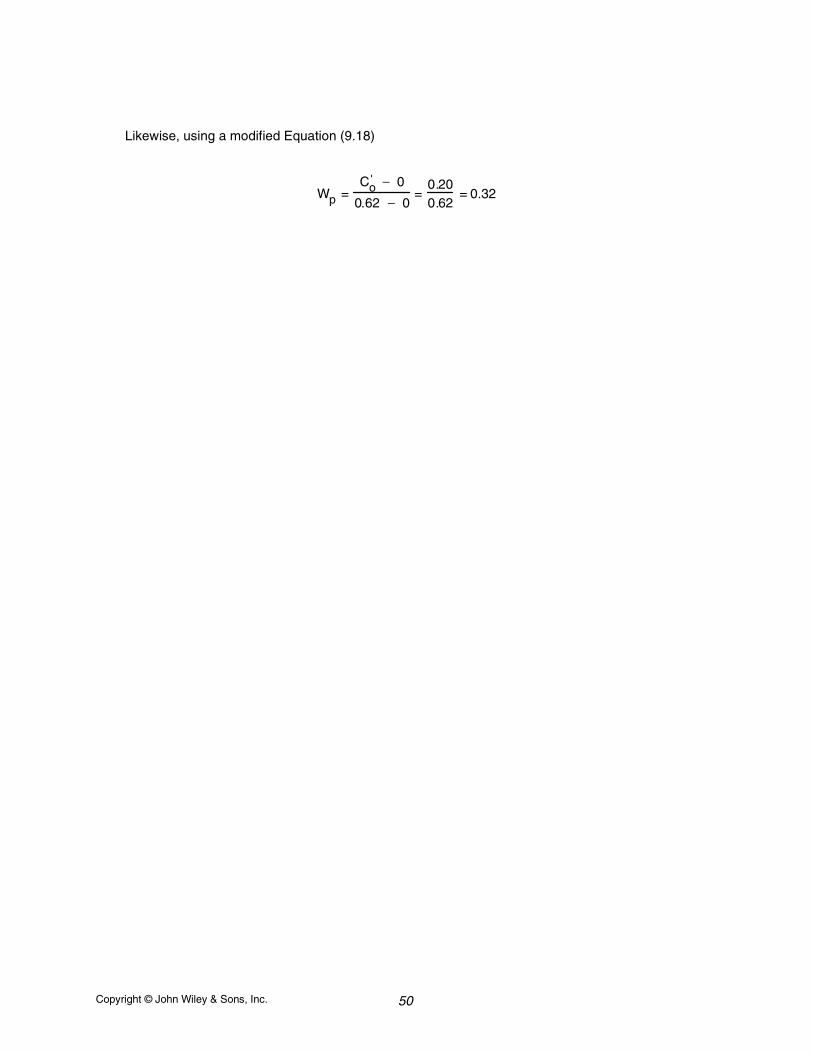
Likewise, using a modified Equation (9.18)
Wp =Co
' − 0
0.62 − 0=
0.200.62
= 0.32
Copyright © John Wiley & Sons, Inc. 51
CHAPTER 10
PHASE TRANSFORMATIONS IN METALS
PROBLEM SOLUTIONS
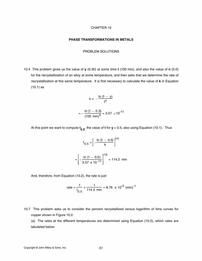
10.4 This problem gives us the value of y (0.30) at some time t (100 min), and also the value of n (5.0)
for the recrystallization of an alloy at some temperature, and then asks that we determine the rate of
recrystallization at this same temperature. It is first necessary to calculate the value of k in Equation
(10.1) as
k = −ln (1 − y)
tn
= −ln (1 − 0.3)
(100 min)5 = 3.57 × 10⁻¹¹
At this point we want to compute t0.5, the value of t for y = 0.5, also using Equation (10.1). Thus
t0.5 = −ln (1 − 0.5)
k
1/n
= −ln (1 − 0.5)
3.57 x 10⁻¹¹
1/5
= 114.2 min
And, therefore, from Equation (10.2), the rate is just
rate =1
t0.5
=1
114.2 min= 8.76 x 10⁻³ (min)-1
10.7 This problem asks us to consider the percent recrystallized versus logarithm of time curves for
copper shown in Figure 10.2.
(a) The rates at the different temperatures are determined using Equation (10.2), which rates are
tabulated below:
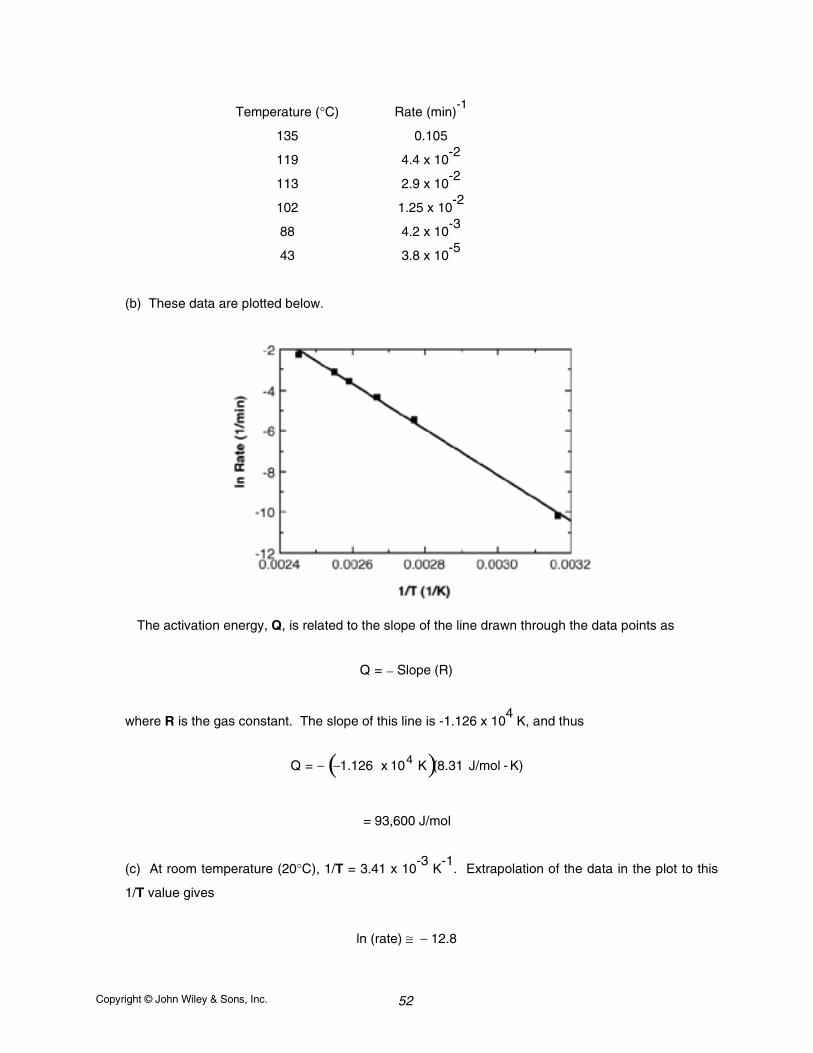
Copyright © John Wiley & Sons, Inc. 52
Temperature (°C) Rate (min)-1
135 0.105
119 4.4 x 10⁻²
113 2.9 x 10⁻²
102 1.25 x 10⁻²
88 4.2 x 10⁻³
43 3.8 x 10⁻⁵
(b) These data are plotted below.
The activation energy, Q, is related to the slope of the line drawn through the data points as
Q = − Slope (R)
where R is the gas constant. The slope of this line is -1.126 x 10⁴ K, and thus
Q = − −1.126 x 10⁴ K( )(8.31 J/mol - K)
= 93,600 J/mol
(c) At room temperature (20°C), 1/T = 3.41 x 10⁻³
K-1
. Extrapolation of the data in the plot to this
1/T value gives
ln (rate) ≅ − 12.8
Copyright © John Wiley & Sons, Inc. 53
which leads to
rate ≅ exp (−12.8) = 2.76 x 10⁻⁶ (min)-1
But since
rate =1
t0.5
then
t0.5 =1
rate=
1
2.76 x 10⁻⁶ (min)−1
= 3.62 x 10⁵ min = 250 days
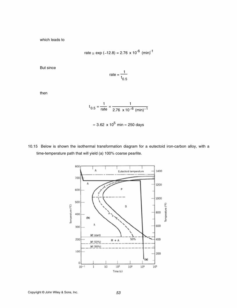
10.15 Below is shown the isothermal transformation diagram for a eutectoid iron-carbon alloy, with a
time-temperature path that will yield (a) 100% coarse pearlite.
Copyright © John Wiley & Sons, Inc. 54
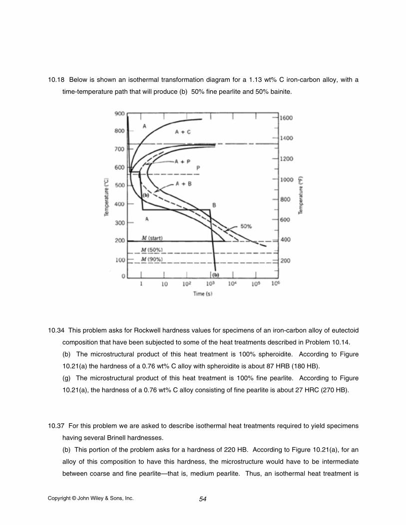
10.18 Below is shown an isothermal transformation diagram for a 1.13 wt% C iron-carbon alloy, with a
time-temperature path that will produce (b) 50% fine pearlite and 50% bainite.
10.34 This problem asks for Rockwell hardness values for specimens of an iron-carbon alloy of eutectoid
composition that have been subjected to some of the heat treatments described in Problem 10.14.
(b) The microstructural product of this heat treatment is 100% spheroidite. According to Figure
10.21(a) the hardness of a 0.76 wt% C alloy with spheroidite is about 87 HRB (180 HB).
(g) The microstructural product of this heat treatment is 100% fine pearlite. According to Figure
10.21(a), the hardness of a 0.76 wt% C alloy consisting of fine pearlite is about 27 HRC (270 HB).
10.37 For this problem we are asked to describe isothermal heat treatments required to yield specimens
having several Brinell hardnesses.
(b) This portion of the problem asks for a hardness of 220 HB. According to Figure 10.21(a), for an
alloy of this composition to have this hardness, the microstructure would have to be intermediate
between coarse and fine pearlite—that is, medium pearlite. Thus, an isothermal heat treatment is
Copyright © John Wiley & Sons, Inc. 55
necessary at a temperature in between those at which fine and coarse pearlites form—for example,
about 630°C. At this temperature, an isothermal heat treatment for at least 25 s is required.
10.D1 This problem inquires as to the possibility of producing an iron-carbon alloy of eutectoid
composition that has a minimum hardness of 200 HB and a minimum ductility of 25%RA. If the alloy
is possible, then the continuous cooling heat treatment is to be stipulated.
According to Figures 10.21(a) and (b), the following is a tabulation of Brinell hardnesses and
percents reduction of area for fine and coarse pearlites and spheroidite for a 0.76 wt% C alloy.
Microstructure HB %RA
Fine pearlite 270 22
Coarse pearlite 205 29
Spheroidite 180 68
Therefore, coarse pearlite meets both of these criteria. The continuous cooling heat treatment which
will produce coarse pearlite for an alloy of eutectoid composition is indicated in Figure 10.18. The
cooling rate would need to be considerably less than 35°C/s, probably on the order of 0.1°C/s.
Copyright © John Wiley & Sons, Inc. 56
CHAPTER 11
APPLICATIONS AND PROCESSING OF METAL ALLOYS
PROBLEM SOLUTIONS
11.5 We are asked to compute the volume percent graphite in a 3.5 wt% C cast iron. It first becomes
necessary to compute mass fractions using the lever rule. From the iron-carbon phase diagram
(Figure 11.2), the tie-line in the αααα and graphite phase field extends from essentially 0 wt% C to 100
wt% C. Thus, for a 3.5 wt% C cast iron
Wα = CGr − CoCGr − Cα
= 100 − 3.5100 − 0
= 0.965
WGr = Co − CαCGr − Cα
= 3.5 − 0100 − 0
= 0.035
Conversion from weight fraction to volume fraction of graphite is possible using Equation (9.6a) as
VGr =
WGrρGr
Wαρα
+WGrρGr
=
0.035
2.3 g /cm3
0.965
7.9 g /cm3+
0.035
2.3 g / cm3
= 0.111 or 11.1 vol%
11.D14 We are to determine, for a cylindrical piece of 8660 steel, the minimum allowable diameter
possible in order yield a surface hardness of 58 HRC, when the quenching is carried out in
moderately agitated oil.
Copyright © John Wiley & Sons, Inc. 57
From Figure 11.14, the equivalent distance from the quenched end of an 8660 steel to give
a hardness of 58 HRC is about 18 mm (3/4 in.). Thus, the quenching rate at the surface of the
specimen should correspond to this equivalent distance. Using Figure 11.16(b), the surface
specimen curve takes on a value of 18 mm equivalent distance at a diameter of about 95 mm (3.75
in.).
Copyright © John Wiley & Sons, Inc. 58
CHAPTER 12
STRUCTURES AND PROPERTIES OF CERAMICS
PROBLEM SOLUTIONS
12.5 This problem calls for us to predict crystal structures for several ceramic materials on the basis of
ionic charge and ionic radii.
(a) For CsI, from Table 12.3
rCs+
rI−
= 0.170 nm0.220 nm
= 0.773
Now, from Table 12.2, the coordination number for each cation (Cs+
) is eight, and, using Table 12.4,
the predicted crystal structure is cesium chloride.
(c) For KI, from Table 12.3
rK +
rI−
= 0.138 nm0.220 nm
= 0.627
The coordination number is six (Table 12.2), and the predicted crystal structure is sodium chloride
(Table 12.4).
12.9 This question is concerned with the zinc blende crystal structure in terms of close-packed planes of
anions.
(a) The stacking sequence of close-packed planes of anions for the zinc blende crystal structure will
be the same as FCC (and not HCP) because the anion packing is FCC (Table 12.4).
(b) The cations will fill tetrahedral positions since the coordination number for cations is four (Table
12.4).
(c) Only one-half of the tetrahedral positions will be occupied because there are two tetrahedral
sites per anion, and yet only one cation per anion.
Copyright © John Wiley & Sons, Inc. 59
12.19 (a) We are asked to compute the theoretical density of CsCl. Modifying the result of Problem 3.4,
we get
a = 2r
Cs+ + 2rCl−
3=
2 (0.170 nm) + 2( 0.181 nm)
3
= 0.405 nm = 4.05 x 10⁻⁸ cm
From Equation (12.1)
ρ = n' ACs + ACl( )
VC
NA
= n' ACs + ACl( )
a3 NA
For the CsCl crystal structure, n' = 1 formula unit/unit cell, and thus
ρ = (1 formula unit/unit cell)(132.91 g/mol + 35.45 g/mol)
4.05 x 10⁻⁸ cm( )3 /unit cell
6.023 x 10²³ formula units/mol( )
= 4.20 g/cm3
12.25 We are asked in this problem to compute the atomic packing factor for the CsCl crystal structure.
This requires that we take the ratio of the sphere volume within the unit cell and the total unit cell
volume. From Figure 12.3 there is the equivalent of one Cs and one Cl ion per unit cell; the ionic
radii of these two ions are 0.170 nm and 0.181 nm, respectively (Table 12.3). Thus, the spherevolume, VS, is just
VS = 43
π( ) (0.170 nm)3 + (0.181 nm)3[ ] = 0.0454 nm3
Using a modified form of the result of Problem 3.4, for CsCl we may express the unit cell edge
length, a, in terms of the atomic radii as
a = 2r
Cs+ + 2rCl-
3 =
2(0.170 nm) + 2(0.181 nm)
3
Copyright © John Wiley & Sons, Inc. 60
= 0.405 nm
Since VC = a3
VC = (0.405 nm)3 = 0.0664 nm3
And, finally the atomic packing factor is just
APF =VSVC
=0.0454 nm3
0.0664 nm3 = 0.684
12.33 (a) For Li+
substituting for Ca2+
in CaO, oxygen vacancies would be created. For each Li+
substituting for Ca2+
, one positive charge is removed; in order to maintain charge neutrality, a
single negative charge may be removed. Negative charges are eliminated by creating oxygen
vacancies, and for every two Li+
ions added, a single oxygen vacancy is formed.
12.38 We are asked for the critical crack tip radius for an Al2O
3 material. From Equation (8.1)
σm = 2 σoa
ρt
1/ 2
Fracture will occur when σσσσm reaches the fracture strength of the material, which is given as E/10;
thus
E10
= 2σoa
ρt
1/ 2
Or, solving for ρρρρt
ρt =400 aσo
2
E 2
From Table 12.5, E = 393 GPa, and thus,
Copyright © John Wiley & Sons, Inc. 61
ρt =(400) 2 x 10⁻³ mm( )(275 MPa)2
393 x 103 MPa( )2
= 3.9 x 10⁻⁷ mm = 0.39 nm
12.42 For this problem, the load is given at which a circular specimen of aluminum oxide fractures when
subjected to a three-point bending test; we are then are asked to determine the load at which a
specimen of the same material having a square cross-section fractures. It is first necessary to
compute the flexural strength of the alumina using Equation (12.3b), and then, using this value, wemay calculate the value of Ff in Equation (12.3a). From Equation (12.3b)
σ fs =FfL
πR3
=(3000 N) 40 x 10−3 m( )
(π) 5.0 x 10⁻³ m( )3= 306 x 106 N/m2 = 306 MPa (42,970 psi)
Now, solving for Ff from Equation (12.3a), realizing that b = d = 12 mm, yields
Ff =2σ fsd3
3L
=(2) 306 x 106 N/m2( )15 x 10−3m( )3
(3) 40 x 10−3 m( ) = 17,200 N (3870 lbf )
12.47 (a) This part of the problem asks us to determine the flexural strength of nonporous MgO
assuming that the value of n in Equation (12.6) is 3.75. Taking natural logarithms of both sides of
Equation (12.6) yields
lnσfs = lnσo − nP
Copyright © John Wiley & Sons, Inc. 62
In Table 12.5 it is noted that for P = 0.05, σσσσfs = 105 MPa. For the nonporous material P = 0 and,
ln σσσσo = ln σσσσfs. Solving for ln σσσσo from the above equation and using these data gives
lnσo = lnσ fs + nP
= ln (105 MPa) + (3.75)(0.05) = 4.841
or σσσσo = e4.841 = 127 MPa (18,100 psi)
(b) Now we are asked to compute the volume percent porosity to yield a σσσσfs of 74 MPa (10,700 psi).
Taking the natural logarithm of Equation (12.6) and solving for P leads to
P =ln σo − ln σ fs
n
= ln (127 MPa) − ln (74 MPa)
3.75
= 0.144 or 14.4 vol%
Copyright © John Wiley & Sons, Inc. 63
CHAPTER 13
APPLICATIONS AND PROCESSING OF CERAMICS
PROBLEM SOLUTIONS
13.5 (a) From Figure 12.25, the maximum temperature without a liquid phase corresponds to the
temperature at the MgO(ss)-[MgO(ss) + Liquid] boundary at this composition, which is approximately
2240°C (4060°F).
13.7 This problem calls for us to compute the mass fractions of liquid for two fireclay refractory materialsat 1600°C. In order to solve this problem it is necessary that we use the SiO2-Al2O3 phase diagram
(Figure 12.27). The mass fraction of liquid, WL, as determined using the lever rule and tie line at
1600°C, is just
WL = Cmullite − CoCmullite − CL
where Cmullite = 72 wt% Al2O3 and CL = 8 wt% Al2O3, as determined using the tie-line; also, Cois the composition (in weight percent Al2O3) of the refractory material.
(a) For the 25 wt% Al2O3- 75 wt% SiO2 composition, Co = 25 wt% Al2O3, and
WL = 72 − 2572 − 8
= 0.73
13.16 (a) Below is shown the logarithm viscosity versus reciprocal of temperature plot for the borosilicate
glass, using the data in Figure 13.6.
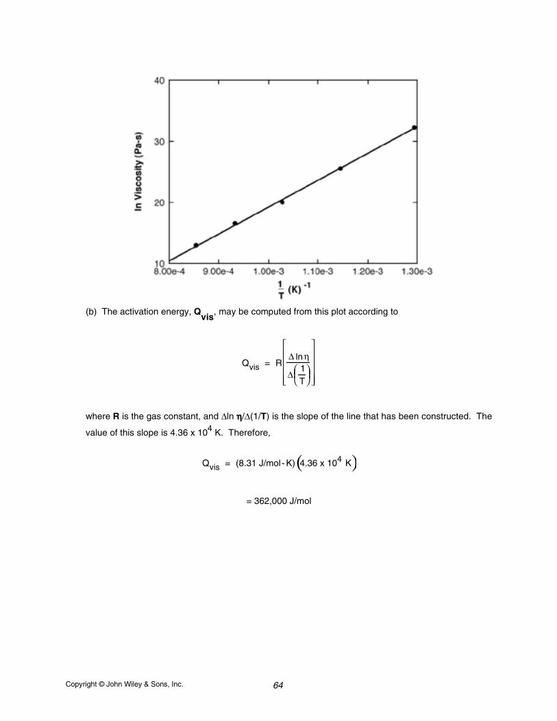
Copyright © John Wiley & Sons, Inc. 64
(b) The activation energy, Qvis
, may be computed from this plot according to
Qvis = R∆ lnη
∆1T
where R is the gas constant, and ∆ln ηηηη/∆(1/T) is the slope of the line that has been constructed. The
value of this slope is 4.36 x 10⁴ K. Therefore,
Qvis = (8.31 J/mol- K) 4.36 x 10⁴ K( )
= 362,000 J/mol
Copyright © John Wiley & Sons, Inc. 65
CHAPTER 14
POLYMER STRUCTURES
PROBLEM SOLUTIONS
14.4 We are asked to compute the number-average degree of polymerization for polypropylene, given
that the number-average molecular weight is 1,000,000 g/mol. The mer molecular weight of
polypropylene is just
m = 3(AC) + 6(AH)
= (3)(12.01 g/mol) + (6)(1.008 g/mol) = 42.08 g/mol
If we let nn
represent the number-average degree of polymerization, then from Equation (14.4a)
nn =M nm
=106 g/mol
42.08 g/mol= 23, 700
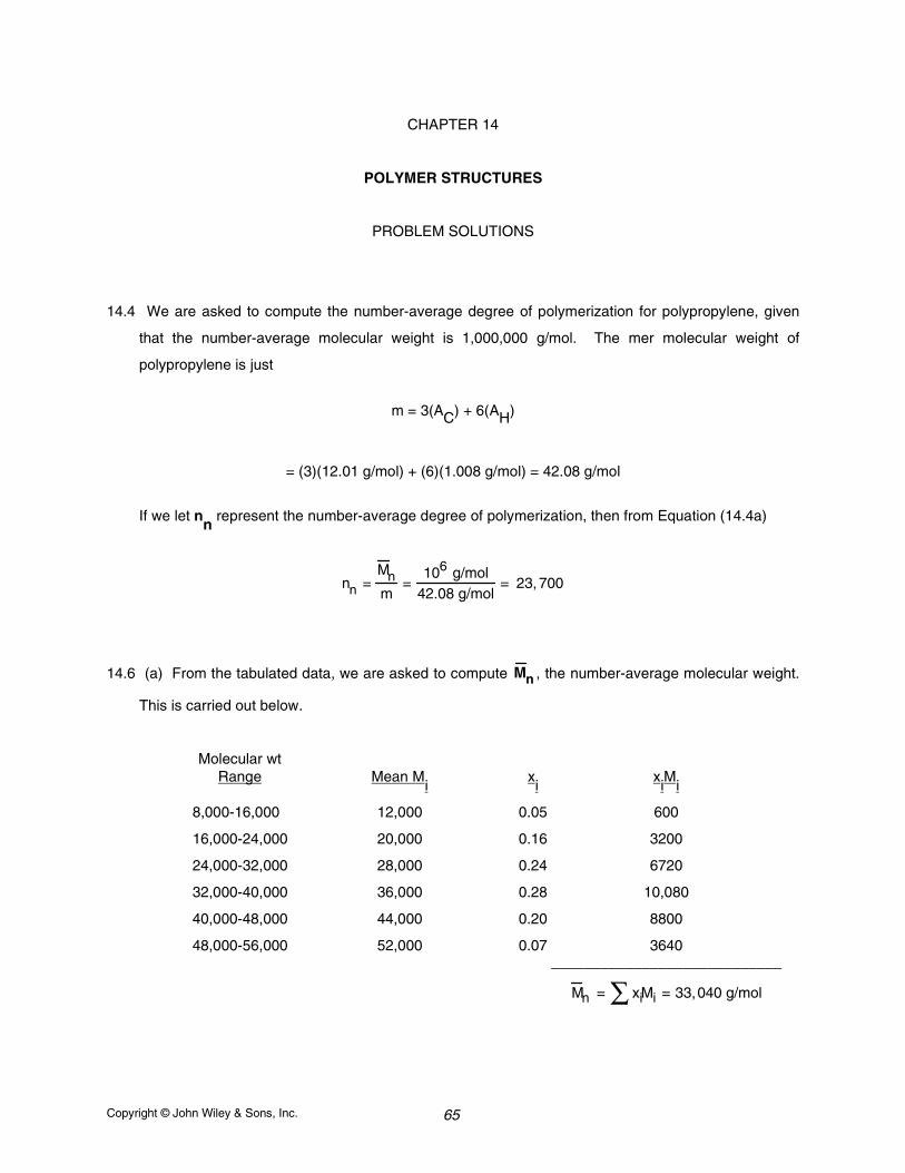
14.6 (a) From the tabulated data, we are asked to compute M n , the number-average molecular weight.
This is carried out below.
Molecular wtRange Mean M
ixi
xiM
i
8,000-16,000 12,000 0.05 600
16,000-24,000 20,000 0.16 3200
24,000-32,000 28,000 0.24 6720
32,000-40,000 36,000 0.28 10,080
40,000-48,000 44,000 0.20 8800
48,000-56,000 52,000 0.07 3640____________________________
M n = xiMi∑ = 33,040 g/mol
Copyright © John Wiley & Sons, Inc. 66
(c) Now we are asked to compute nn
(the number-average degree of polymerization), using the
Equation (14.4a). For polypropylene,
m = 3(AC) + 6(AH)
= (3)(12.01 g/mol) + (6)(1.008 g/mol) = 42.08 g/mol
And
nn =M nm
=33,040 g/mol42.08 g/mol
= 785
14.11 This problem first of all asks for us to calculate, using Equation (14.11), the average total chain
length, L, for a linear polyethylene polymer having a number-average molecular weight of 300,000g/mol. It is necessary to calculate the number-average degree of polymerization, nn, using
Equation (14.4a). For polyethylene, from Table 14.3, each mer unit has two carbons and four
hydrogens. Thus,
m = 2(AC) + 4(AH)
= (2)(12.01 g/mol) + (4)(1.008 g/mol) = 28.05 g/mol
and
nn = M nm
= 300,000 g/mol
28.05 g/mol = 10,695
which is the number of mer units along an average chain. Since there are two carbon atoms per mer
unit, there are two C--C chain bonds per mer, which means that the total number of chain bonds in
the molecule, N, is just (2)(10,695) = 21,390 bonds. Furthermore, assume that for single carbon-
carbon bonds, d = 0.154 nm and θθθθ = 109° (Section 14.4); therefore, from Equation (14.11)
L = Nd sin θ2
= (21,390)(0.154 nm) sin 109°
2
= 2682 nm
Copyright © John Wiley & Sons, Inc. 67
It is now possible to calculate the average chain end-to-end distance, r, using Equation
(14.12) as
r = d N = (0.154 nm) 21,390 = 22.5 nm
14.28 Given that polyethylene has an orthorhombic unit cell with two equivalent mer units, we are asked
to compute the density of totally crystalline polyethylene. In order to solve this problem it is
necessary to employ Equation (3.5), in which n represents the number of mer units within the unit
cell (n = 2), and A is the mer molecular weight, which for polyethylene is just
A = 2(AC) + 4(AH)
= (2)(12.01 g/mol) + (4)(1.008 g/mol) = 28.05 g/mol
Also, VC is the unit cell volume, which is just the product of the three unit cell edge lengths as shown
in Figure 14.10. Thus,
ρ = nA
VC
NA
= (2 mers/uc)(28.05 g/mol)
7.41 x 10⁻⁸ cm( )4.94 x 10⁻⁸ cm( )2.55 x 10⁻⁸ cm( )/uc
6.023 x 10²³ mers/mol( )
= 0.998 g/cm3
Copyright © John Wiley & Sons, Inc. 68
CHAPTER 15
CHARACTERISTICS, APPLICATIONS, AND PROCESSING OF POLYMERS
PROBLEM SOLUTIONS
15.15 This problem gives us the tensile strengths and associated number-average molecular
weights for two polymethyl methacrylate materials and then asks that we estimate the tensilestrength for M n = 30,000 g/mol. Equation (15.3) provides the dependence of the tensile
strength on M n . Thus, using the data provided in the problem, we may set up two
simultaneous equations from which it is possible to solve for the two constants TS• and A.
These equations are as follows:
107 MPa = TS∞ −A
40,000 g /mol
170 MPa = TS∞ −A
60,000 g /mol
Thus, the values of the two constants are: TS• = 296 MPa and A = 7.56 x 10⁶ MPa-g/mol.
Substituting these values into the equation for which M n = 30,000 g/mol leads to
TS = TS∞ −A
30,000 g /mol
= 296 MPa − 7.56 x 10⁶ MPa - g /mol
30,000 g /mol
= 44 MPa
15.24 This problem asks that we compute the fraction of possible crosslink sites in 10 kg of
polybutadiene when 4.8 kg of S is added, assuming that, on the average, 4.5 sulfur atoms
participate in each crosslink bond. Given the butadiene mer unit in Table 14.5, we may
calculate its molecular weight as follows:
Copyright © John Wiley & Sons, Inc. 69
A(butadiene) = 4(AC) + 6(AH)
= (4)(12.01 g/mol) + 6(1.008 g/mol) = 54.09 g/mol
Which means that in 10 kg of butadiene there are 10,000 g
54.09 g /mol = 184.9 mol.
For the vulcanization of polybutadiene, there are two possible crosslink sites per
mer--one for each of the two carbon atoms that are doubly bonded. Furthermore, each of
these crosslinks forms a bridge between two mers. Therefore, we can say that there is the
equivalent of one crosslink per mer. Therefore, let us now calculate the number of moles ofsulfur (nsulfur) that react with the butadiene, by taking the mole ratio of sulfur to butadiene,
and then dividing this ratio by 4.5 atoms per crosslink; this yields the fraction of possible
sites that are crosslinked. Thus
nsulfur =4800 g
32.06 g /mol= 149.7 mol
And
fraction sites crosslinked =
149.7 mol184.9 mol
4.5= 0.180
15.42 (a) This problem asks that we determine how much ethylene glycol must be added to 20.0
kg of adipic acid to produce a linear chain structure of polyester according to Equation 15.9.
Since the chemical formulas are provided in this equation we may calculate the molecular
weights of each of these materials as follows:
A(adipic) = 6(AC) + 10(AH) + 4(AO)
= 6(12.01 g/mol) + 10(1.008 g/mol) + 4 (16.00 g/mol) = 146.14 g/mol
A(glycol) = 2(AC ) + 6(AH) + 2(AO)
= 2(12.01 g/mol) + 6(1.008 g/mol) + 2(16.00 g/mol) = 62.07 g/mol
Copyright © John Wiley & Sons, Inc. 70
The 20.0 kg mass of adipic acid equals 20,000 g or 20,000 g
146.14 g /mol = 136.86 mol. Since,
according to Equation (15.9), each mole of adipic acid used requires one mole of ethylene
glycol, which is equivalent to (136.86 mol)(62.07 g/mol) = 8495 g = 8.495 kg.
(b) Now we are asked for the mass of the resulting polyester. Inasmuch as one mole of
water is given off for every mer unit produced, this corresponds to 136.86 moles or (136.86
mol)(18.02 g/mol) = 2466 g or 2.466 kg since the molecular weight of water is 18.02 g/mol.
The mass of polyester is just the sum of the masses of the two reactant materials [as
computed in part (a)] minus the mass of water released, or
mass(polyester) = 20.0 kg + 8.495 kg − 2.466 kg = 26.03 kg
Copyright © John Wiley & Sons, Inc. 71
CHAPTER 16
COMPOSITES
PROBLEM SOLUTIONS
16.4 This problem asks for the maximum and minimum thermal conductivity values for a TiC-Co cermet.Using a modified form of Equation (16.1) the maximum thermal conductivity kmax is calculated as
kmax = kmVm + kpVp = kCoVCo + kTiCVTiC
= (69 W/m - K)(0.15) + (27 W/m -K)(0.85) = 33.3 W/m -K
And, from a modified form of Equation (16.2), the minimum thermal conductivity kmin is
kmin =kCokTiC
VCokTiC + VTiCkCo
= (69 W /m - K)(27 W /m -K)
(0.15)(27 W /m- K) + (0.85)(69 W /m -K)
= 29.7 W/m-K
16.12 This problem asks for us to determine if it is possible to produce a continuous and oriented aramid
fiber-epoxy matrix composite having longitudinal and transverse moduli of elasticity of 35 GPa and
5.17 GPa, respectively, given that the modulus of elasticity for the epoxy is 3.4 GPa. Also, from
Table 16.4 the value of E for aramid fibers is 131 GPa. The approach to solving this problem is tocalculate two values of Vf using the data and Equations (16.10b) and (16.16); if they are the same
then this composite is possible.For the longitudinal modulus Ecl,
Ecl = Em 1 - Vfl( ) + EfVfl
35 GPa = (3.4 GPa) 1 - Vfl( ) + (131 GPa)Vfl
Copyright © John Wiley & Sons, Inc. 72
Solving this expression for Vfl yields Vfl = 0.248.
Now, repeating this procedure for the transverse modulus Ect
Ect = EmEf
1 − Vft( )Ef+ VftEm
5.17 GPa = (3.4 GPa)(131 GPa)
1 − Vft( )(131 GPa) + Vft(3.4 GPa)
Solving this expression for Vft leads to Vft = 0.351. Thus, since Vfl and Vft are not equal, the
proposed composite is not possible.
16.17 This problem stipulates that the cross-sectional area of a composite, Ac, is 320 mm
2 (0.50 in.
2),
and that the longitudinal load, Fc, is 44,500 N (10,000 lbf) for the composite described in Problem
16.11.(a) First, we are asked to calculate the F
f/F
m ratio. According to Equation (16.11)
FfFm
= EfVf
EmVm=
(131 GPa)(0.30)(2.4 GPa)(0.70)
= 23.4
Or, Ff = 23.4F
m
(b) Now, the actual loads carried by both phases are called for. Since
Ff + Fm = Fc = 44,500 N
23.4Fm + Fm = 44,500 N
which leads toFm = 1824 N (410 lbf )
Ff = 44,500 N − 1824 N = 42,676 N (9590 lb f)
(c) To compute the stress on each of the phases, it is first necessary to know the cross-sectional
areas of both fiber and matrix. These are determined as
Copyright © John Wiley & Sons, Inc. 73
A f = Vf Ac = (0.30)(320 mm2) = 96 mm2 (0.15 in.2)
Am = VmAc = (0.70)(320 mm2) = 224 mm2 (0.35 in.2)
Now, for the stresses,
σ f = FfA f
= 42,676 N
96 mm2=
42,676 N
96 x 10−6 m2 = 445 MPa (63,930 psi)
σm = FmAm
= 1824 N
224 mm2 =1824 N
224 x 10-6 m2 = 8.14 MPa (1170 psi)
(d) The strain on the composite is the same as the strain on each of the matrix and fiber phases, as
εm = σmEm
= 8.14 MPa
2.4 x 10³ MPa= 3.39 x 10⁻³
εf = σfEf
= 445 MPa
131 x 103 MPa= 3.39 x 10⁻³
16.21 In this problem, for an aligned glass fiber-epoxy matrix composite, we are asked to compute the
longitudinal tensile strength given the following: the average fiber diameter (0.015 mm), the average
fiber length (2.0 mm), the volume fraction of fibers (0.25), the fiber fracture strength (3500 MPa), the
fiber-matrix bond strength (100 MPa), and the matrix stress at composite failure (5.5 MPa). It is first
necessary to compute the value of the critical fiber length using Equation (16.3). If the fiber length is
much greater than lc, then we may determine σσσσcl∗ using Equation (16.17), otherwise, use of either
Equation (16.18) or (16.19) is necessary. Thus,
lc = σ f
∗ d
2τc=
(3500 MPa)(0.015 mm)2(100 MPa)
= 0.263 mm (0.010 in.)
Inasmuch as l > lc (2.0 mm > 0.263 mm), but l is not much greater than lc, then use of Equation
(16.18) is necessary. Therefore,
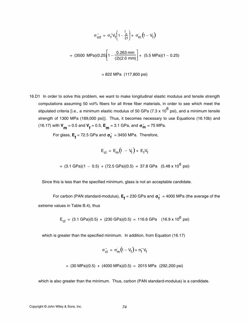
Copyright © John Wiley & Sons, Inc. 74
σcd∗ = σ f
∗Vf 1 −lc2 l
+ σm
' 1 − Vf( )
= (3500 MPa)(0.25) 1 −0.263 mm
(2)(2.0 mm)
+ (5.5 MPa)(1 − 0.25)
= 822 MPa (117,800 psi)
16.D1 In order to solve this problem, we want to make longitudinal elastic modulus and tensile strength
computations assuming 50 vol% fibers for all three fiber materials, in order to see which meet the
stipulated criteria [i.e., a minimum elastic modulus of 50 GPa (7.3 x 10⁶ psi), and a minimum tensile
strength of 1300 MPa (189,000 psi)]. Thus, it becomes necessary to use Equations (16.10b) and
(16.17) with Vm
= 0.5 and Vf = 0.5, E
m = 3.1 GPa, and σσσσm
∗ = 75 MPa.
For glass, Ef = 72.5 GPa and σσσσ f
∗ = 3450 MPa. Therefore,
Ecl = Em 1 − Vf( ) + EfVf
= (3.1 GPa)(1 − 0.5) + (72.5 GPa)(0.5) = 37.8 GPa (5.48 x 10⁶ psi)
Since this is less than the specified minimum, glass is not an acceptable candidate.
For carbon (PAN standard-modulus), Ef = 230 GPa and σσσσ f∗ = 4000 MPa (the average of the
extreme values in Table B.4), thus
Ecl = (3.1 GPa)(0.5) + (230 GPa)(0.5) = 116.6 GPa (16.9 x 10⁶ psi)
which is greater than the specified minimum. In addition, from Equation (16.17)
σcl∗ = σm
' 1 − Vf( )+ σf∗ Vf
= (30 MPa)(0.5) + (4000 MPa)(0.5) = 2015 MPa (292,200 psi)
which is also greater than the minimum. Thus, carbon (PAN standard-modulus) is a candidate.
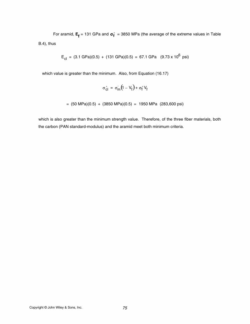
Copyright © John Wiley & Sons, Inc. 75
For aramid, Ef = 131 GPa and σσσσ f∗ = 3850 MPa (the average of the extreme values in Table
B.4), thus
Ecl = (3.1 GPa)(0.5) + (131 GPa)(0.5) = 67.1 GPa (9.73 x 10⁶ psi)
which value is greater than the minimum. Also, from Equation (16.17)
σcl∗ = σm
' 1 − Vf( )+ σf∗ Vf
= (50 MPa)(0.5) + (3850 MPa)(0.5) = 1950 MPa (283,600 psi)
which is also greater than the minimum strength value. Therefore, of the three fiber materials, both
the carbon (PAN standard-modulus) and the aramid meet both minimum criteria.
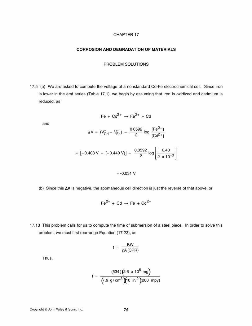
Copyright © John Wiley & Sons, Inc. 76
CHAPTER 17
CORROSION AND DEGRADATION OF MATERIALS
PROBLEM SOLUTIONS
17.5 (a) We are asked to compute the voltage of a nonstandard Cd-Fe electrochemical cell. Since iron
is lower in the emf series (Table 17.1), we begin by assuming that iron is oxidized and cadmium is
reduced, as
Fe + Cd2+ → Fe2+ + Cd
and
∆V = (VCd − VFe) − 0.0592
2log
[Fe2+ ]
[Cd2+ ]
= − 0.403 V − (− 0.440 V)[ ] − 0.0592
2log
0.40
2 x 10−3
= -0.031 V
(b) Since this ∆∆∆∆V is negative, the spontaneous cell direction is just the reverse of that above, or
Fe2+ + Cd → Fe + Cd2+
17.13 This problem calls for us to compute the time of submersion of a steel piece. In order to solve this
problem, we must first rearrange Equation (17.23), as
t = KW
ρA (CPR)
Thus,
t = (534 ) 2.6 x 10⁶ mg( )
7.9 g / cm3( )10 in.2( )(200 mpy)
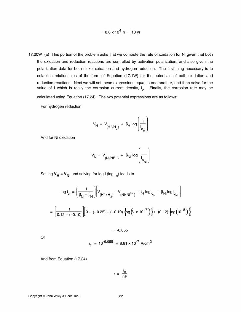
Copyright © John Wiley & Sons, Inc. 77
= 8.8 x 10⁴ h = 10 yr
17.20W (a) This portion of the problem asks that we compute the rate of oxidation for Ni given that both
the oxidation and reduction reactions are controlled by activation polarization, and also given the
polarization data for both nickel oxidation and hydrogen reduction. The first thing necessary is to
establish relationships of the form of Equation (17.1W) for the potentials of both oxidation and
reduction reactions. Next we will set these expressions equal to one another, and then solve for thevalue of i which is really the corrosion current density, ic. Finally, the corrosion rate may be
calculated using Equation (17.24). The two potential expressions are as follows:
For hydrogen reduction
VH = V(H+/H
2) + βH log
iio
H
And for Ni oxidation
VNi = V(Ni/Ni2+ )
+ βNi log i
ioNi
Setting VH = VNi and solving for log i (log ic) leads to
log ic = 1
βNi
− βH
V
(H+ / H2
)− V
(Ni/ Ni2+ )− βH logio
H+ βNi logio
Ni
= 1
0.12 − (−0.10)
0 − (− 0.25) − (−0.10) log 6 x 10⁻⁷( ) + (0.12) log 10−8( )
= -6.055
Or
ic = 10-6.055 = 8.81 x 10⁻⁷ A/cm2
And from Equation (17.24)
r = icnF
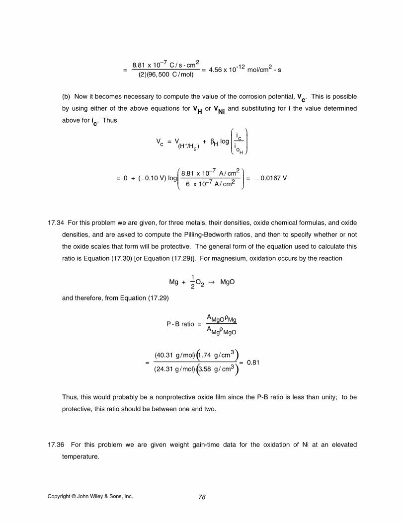
Copyright © John Wiley & Sons, Inc. 78
= 8.81 x 10⁻⁷ C / s - cm2
(2)(96,500 C /mol)= 4.56 x 10⁻¹² mol/cm2 - s
(b) Now it becomes necessary to compute the value of the corrosion potential, Vc. This is possible
by using either of the above equations for VH or VNi and substituting for i the value determined
above for ic. Thus
Vc = V(H+/H
2) + βH log
icio
H
= 0 + (−0.10 V) log8.81 x 10−7 A / cm2
6 x 10⁻⁷ A/ cm2
= − 0.0167 V
17.34 For this problem we are given, for three metals, their densities, oxide chemical formulas, and oxide
densities, and are asked to compute the Pilling-Bedworth ratios, and then to specify whether or not
the oxide scales that form will be protective. The general form of the equation used to calculate this
ratio is Equation (17.30) [or Equation (17.29)]. For magnesium, oxidation occurs by the reaction
Mg + 12
O2 → MgO
and therefore, from Equation (17.29)
P - B ratio = AMgOρMg
AMgρ
MgO
= (40.31 g /mol) 1.74 g /cm3( )(24.31 g /mol) 3.58 g / cm3( )= 0.81
Thus, this would probably be a nonprotective oxide film since the P-B ratio is less than unity; to be
protective, this ratio should be between one and two.
17.36 For this problem we are given weight gain-time data for the oxidation of Ni at an elevated
temperature.
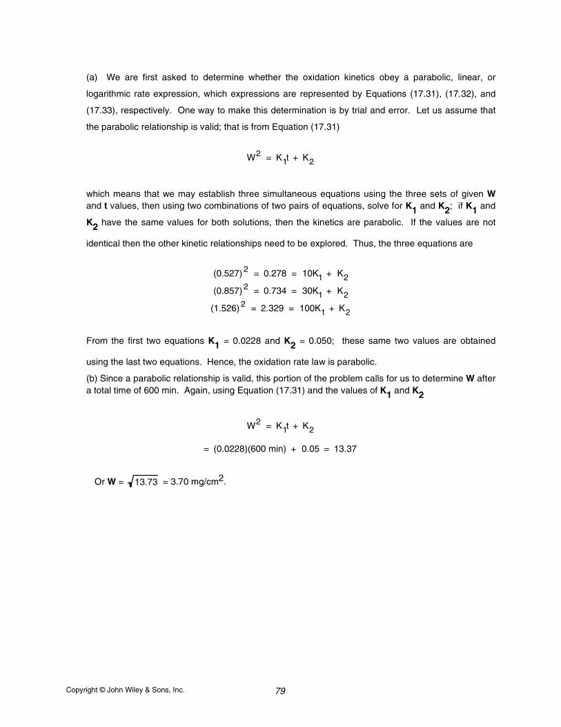
Copyright © John Wiley & Sons, Inc. 79
(a) We are first asked to determine whether the oxidation kinetics obey a parabolic, linear, or
logarithmic rate expression, which expressions are represented by Equations (17.31), (17.32), and
(17.33), respectively. One way to make this determination is by trial and error. Let us assume that
the parabolic relationship is valid; that is from Equation (17.31)
W2 = K1t + K2
which means that we may establish three simultaneous equations using the three sets of given Wand t values, then using two combinations of two pairs of equations, solve for K1 and K2; if K1 and
K2 have the same values for both solutions, then the kinetics are parabolic. If the values are not
identical then the other kinetic relationships need to be explored. Thus, the three equations are
(0.527) 2 = 0.278 = 10K1 + K2
(0.857) 2 = 0.734 = 30K1 + K2
(1.526) 2 = 2.329 = 100K1 + K2
From the first two equations K1 = 0.0228 and K2 = 0.050; these same two values are obtained
using the last two equations. Hence, the oxidation rate law is parabolic.
(b) Since a parabolic relationship is valid, this portion of the problem calls for us to determine W aftera total time of 600 min. Again, using Equation (17.31) and the values of K1 and K2
W2 = K1t + K2
= (0.0228)(600 min) + 0.05 = 13.37
Or W = 13.73 = 3.70 mg/cm2.
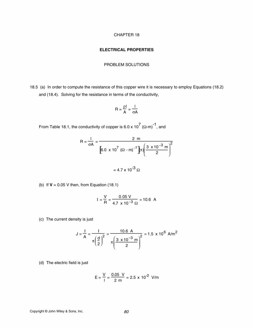
Copyright © John Wiley & Sons, Inc. 80
CHAPTER 18
ELECTRICAL PROPERTIES
PROBLEM SOLUTIONS
18.5 (a) In order to compute the resistance of this copper wire it is necessary to employ Equations (18.2)
and (18.4). Solving for the resistance in terms of the conductivity,
R =ρlA
=l
σA
From Table 18.1, the conductivity of copper is 6.0 x 10⁷ (Ω-m)
-1, and
R =l
σA=
2 m
6.0 x 10⁷
(Ω − m)−1[ ](π)3 x 10⁻³ m
2
2
= 4.7 x 10⁻³ Ω
(b) If V = 0.05 V then, from Equation (18.1)
I =VR
=0.05 V
4.7 x 10⁻³ Ω= 10.6 A
(c) The current density is just
J =I
A=
I
πd2
2 =10.6 A
π 3 x 10⁻³ m2
2 = 1.5 x 10⁶ A/m2
(d) The electric field is just
E =Vl
=0.05 V
2 m= 2.5 x 10⁻² V/m
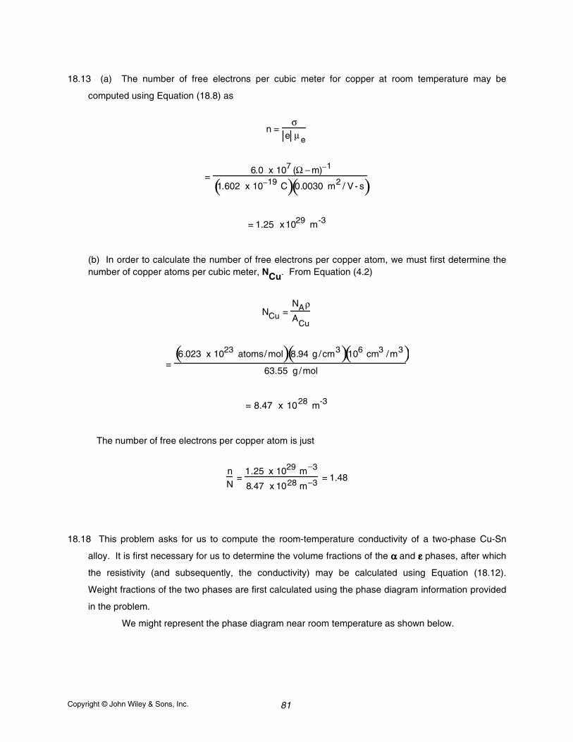
Copyright © John Wiley & Sons, Inc. 81
18.13 (a) The number of free electrons per cubic meter for copper at room temperature may be
computed using Equation (18.8) as
n =σ
e µe
=6.0 x 10⁷ (Ω − m)−1
1.602 x 10⁻¹⁹ C( )0.0030 m2 / V - s( )
= 1.25 x1029 m-3
(b) In order to calculate the number of free electrons per copper atom, we must first determine thenumber of copper atoms per cubic meter, NCu. From Equation (4.2)
NCu =NAρACu
=6.023 x 10²³ atoms/mol( )8.94 g /cm3( )106 cm3 /m3( )
63.55 g /mol
= 8.47 x 1028 m-3
The number of free electrons per copper atom is just
nN
=1.25 x 1029 m−3
8.47 x 1028 m−3 = 1.48
18.18 This problem asks for us to compute the room-temperature conductivity of a two-phase Cu-Sn
alloy. It is first necessary for us to determine the volume fractions of the αααα and εεεε phases, after which
the resistivity (and subsequently, the conductivity) may be calculated using Equation (18.12).
Weight fractions of the two phases are first calculated using the phase diagram information provided
in the problem.
We might represent the phase diagram near room temperature as shown below.
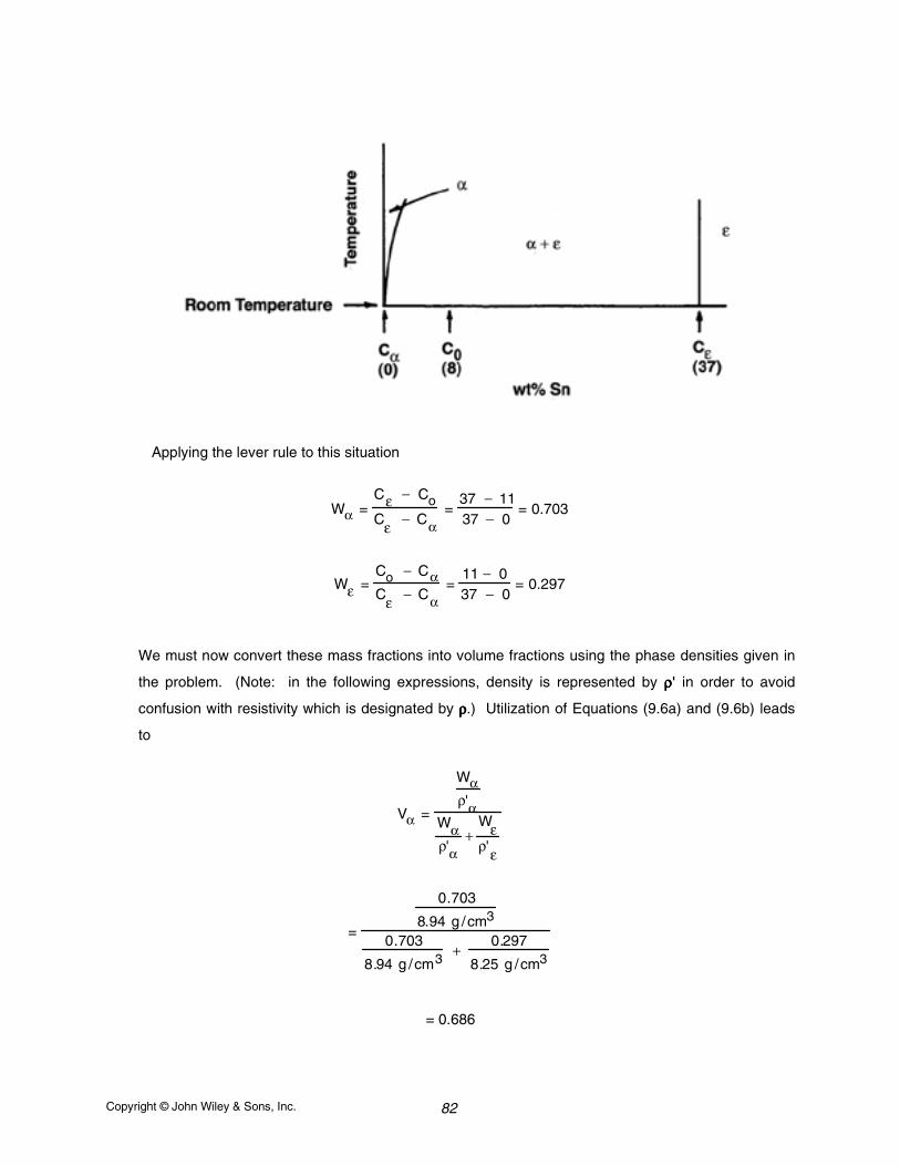
Copyright © John Wiley & Sons, Inc. 82
Applying the lever rule to this situation
Wα =Cε − CoCε − Cα
=37 − 1137 − 0
= 0.703
Wε =Co − CαCε − Cα
=11 − 037 − 0
= 0.297
We must now convert these mass fractions into volume fractions using the phase densities given in
the problem. (Note: in the following expressions, density is represented by ρρρρ' in order to avoid
confusion with resistivity which is designated by ρρρρ.) Utilization of Equations (9.6a) and (9.6b) leads
to
Vα =
Wαρ'α
Wαρ'α
+Wερ'ε
=
0.703
8.94 g /cm3
0.703
8.94 g /cm3+
0.297
8.25 g /cm3
= 0.686
Copyright © John Wiley & Sons, Inc. 83
Vε =
Wερ'ε
Wαρ'α
+Wερ'ε
=
0.297
8.25 g /cm3
0.703
8.94 g /cm3+ 0.297
8.25 g /cm3
= 0.314
Now, using Equation (18.12)
ρ = ραVα + ρεVε
= 1.88 x 10⁻⁸ Ω - m( )(0.686) + 5.32 x 10⁻⁷ Ω - m( )(0.314)
= 1.80 x 10⁻⁷ Ω - m
Finally, for the conductivity [Equation (18.4)]
σ =1ρ
=1
1.80 x 10⁻⁷ Ω − m= 5.56 x10⁶ (Ω - m)-1
18.31 (a) In this problem, for a Si specimen, we are given p and σσσσ, while µµµµh and µµµµe are included in
Table 18.2. In order to solve for n we must use Equation (18.13), which, after rearrangement, leads
to
n =σ − p e µh
e µe
= 103 (Ω − m)−1 − 1.0 x 10²³ m−3( )1.602 x 10⁻¹⁹ C( )0.05 m2 /V - s( )
1.602 x 10⁻¹⁹ C( )0.14 m2 / V - s( )
Copyright © John Wiley & Sons, Inc. 84
= 8.9 x 10²¹ m-3
(b) This material is p-type extrinsic since p (1.0 x 10²³
m-3
) is greater than n (8.9 x 10²¹
m-3
).
18.41 This problems asks that we determine the room-temperature electrical conductivity of silicon that
has been doped with 1023 m-3 of arsenic atoms. Inasmuch as As is a group VA element in the
periodic table (Figure 2.6) it acts as a donor in silicon. Thus, this material is n-type extrinsic, and it
is necessary to use Equation (18.16), with n = 1023 m-3 since at room temperature all of the As
donor impurities are ionized. The electron mobility, from Figure 18.17 at an impurity concentration of
1023 m-3, is 0.065 m2/V-s. Therefore, the conductivity is equal to
σ = n e µe = 1023 m−3( )1.6 x 10⁻¹⁶ C( )0.065 m2 / V − s( )= 1040 (Ω − m)−1
18.47W In this problem we are asked to determine the magnetic field required to produce a Hall voltage
of –3.5 x 10⁻⁷ V, given that σσσσ = 1.2 x 10⁷ (Ω-m)-1, µµµµe = 0.0050 m2/V-s, Ix = 40 A, and d = 35 mm.
Combining Equations (18.1W) and (18.3bW), and after solving for Bz, we get
Bz =VH σd
Ixµe
= −3.5 x 10⁻⁷ V
1.2 x 10⁷ (Ω − m)−1[ ]35 x 10−3 m( )
(40 A) 0.0050 m2 / V - s( )
= 0.74 tesla
18.54W We want to compute the plate spacing of a parallel-plate capacitor as the dielectric constant is
increased form 2.5 to 4.0, while maintaining the capacitance constant. Combining Equations
(18.6W) and (18.7W) yields
C =εrεoA
l
Copyright © John Wiley & Sons, Inc. 85
Now, let us use the subscripts 1 and 2 to denote the initial and final states, respectively. Since C1 =
C2, then
εr1εoA
l1=
εr2εoA
l2
And, solving for l2
l2 = εr2l1ε
r1=
(4.0)(1 mm)2.5
= 1.6 mm
18.60W (a) We want to solve for the voltage when Q = 3.5 x 10⁻¹¹
C, A = 160 mm2, l = 3.5 mm, and εεεεr
= 5.0. Combining Equations (18.4W), (18.6W), and (18.7W) yields
QV
= εrεoAl
And, solving for V
V = Q l
εrε
oA
= 3.5 x 10⁻¹¹ C( )3.5 x 10⁻³ m( )
(5.0) 8.85 x 10⁻¹² F/ m( )160 mm2( )1 m2 /106 mm2( )
= 17.3 V
(b) For this same capacitor, if a vacuum is used
V = Q l
εoA
= 3.5 x 10⁻¹¹ C( )3.5 x 10⁻³ m( )
8.85 x 10⁻¹² F /m( )160 x 10−6 m2( )
= 86.5 V
Copyright © John Wiley & Sons, Inc. 86
(e) The polarization is determined using Equations (18.12W) and (18.6) as
P = εo(εr − 1)Vl
= 8.85 x 10⁻¹² F /m( )(5.0 − 1)(17.3 V)
3.5 x 10⁻³ m
= 1.75 x 10⁻⁷ C/m2
18.D2 This problem asks that we determine the electrical conductivity of an 85 wt% Cu-15 wt% Zn alloy
at -100°C using information contained in Figures 18.8 and 18.28. In order to solve this problem it is
necessary to employ Equation (18.9) which is of the form
ρtotal = ρt + ρi
since it is assumed that the alloy is undeformed. Let us first determine the value of ρρρρi at room
temperature (25°C) which value will be independent of temperature. From Figure (18.8), at 25°C
and for pure Cu, ρρρρt(25) = 1.75 x 10⁻⁸ Ω-m. Now, since it is assumed that the curve in Figure 18.28
was generated also at room temperature, we may take ρρρρ as ρρρρtotal(25) at 85 wt% Cu-15 wt% Zn
which has a value of 4.7 x 10⁻⁸ Ω-m. Thus
ρi = ρtotal(25) − ρt(25)
= 4.7 x 10⁻⁸ Ω - m - 1.75 x 10⁻⁸ Ω - m = 2.95 x 10⁻⁸ Ω - m
Finally, we may determine the resistivity at -100°C, ρρρρtotal(-100), by taking the resistivity of pure Cu
at -100°C from Figure 18.8, which gives us ρρρρt(-100) = 0.90 x 10⁻⁸ Ω-m. Therefore
ρtotal (-100) = ρi + ρt(-100)
= 2.95 x 10⁻⁸ Ω - m + 0.90 x 10⁻⁸ Ω - m = 3.85 x 10⁻⁸ Ω - m
And, using Equation (18.4) the conductivity is calculated as
Copyright © John Wiley & Sons, Inc. 87
σ = 1ρ
= 1
3.85 x 10⁻⁸ Ω − m= 2.60 x 10
7 (Ω - m)
-1
Copyright © John Wiley & Sons, Inc. 88
CHAPTER 19
THERMAL PROPERTIES
PROBLEM SOLUTIONS
19.4 (a) For aluminum, Cv at 50
K may be approximated by Equation (19.2), since this temperature is
significantly below the Debye temperature. The value of Cv at 30
K is given, and thus, we may
compute the constant A as
A = CvT3 =
0.81 J/ mol- K
(30 K)3= 3 x 10⁻⁵ J/mol - K4
Therefore, at 50 K
Cv = AT3 = 3 x 10⁻⁵ J/mol -K 4( )(50 K)3 = 3.75 J/mol -K
and
cv = (3.75 J/mol- K)(1 mol/26.98 g)(1000 g/kg) = 139 J/kg - K
19.14 This problem asks for us to determine the temperature to which a cylindrical rod of tungsten
15.025 mm in diameter must be heated in order for it of just fit into a 15.000 mm diameter circular
hole in a plate of 1025 steel (which, of course, is also heated), assuming that the initial temperature
is 25°C. This requires the use of Equation (19.3a), which is applied to the diameters of both the rod
and hole. That is
df − dodo
= α l Tf − To( )
Solving this expression for df yields
df = do 1 + α l Tf − To( )
Copyright © John Wiley & Sons, Inc. 89
Now all we need do is to establish expressions for df(steel) and df(W), set them equal to one
another, and solve for Tf. According to Table 19.1, ααααl(steel) = 12.0 x 10⁻⁶ (°C)-1 and ααααl(W) = 4.5 x
10-6 (°C)-1. Thus
df(steel) = df (W)
(15.000 mm) 1 + 12.0 x 10⁻⁶(°C)−1 Tf − 25°C( )
= (15.025 mm) 1 + 4.5 x 10⁻⁶(°C)−1 Tf − 25°C( )
Now solving for Tf gives Tf = 222.4°C
19.24 This problem asks that we treat a porous material as a composite wherein one of the phases is a
pore phase, and that we estimate upper and lower limits for the room-temperature thermal
conductivity of an aluminum oxide material having a 0.25 volume fraction of pores. The upper limitof k (kupper) may be determined using Equation (16.1) with thermal conductivity substituted for the
elastic modulus, E. From Table 19.1, the value of k for Al2O3 is 39 W/m-K, while for still air in the
pore phase, k = 0.02 W/m-K. Thus
kupper = Vpkair + VAl2O
3kAl
2O
3
= (0.25)(0.02 W/m-K) + (0.75)(39 W/m-K) = 29.3 W/m-K
19.29 We want to heat the copper wire in order to reduce the stress level from 70 MPa to 35 MPa; in
doing so, we reduce the stress in the wire by 70 MPa - 35 MPa = 35 MPa, which stress will be acompressive one (i.e., σσσσ = -35 MPa). Solving for T
f from Equation (19.8)
Tf = To −σ
Eαl
= 20°C − -35 MPa
110 x 103 MPa( )17 x 10−6 (°C)−1[ ]
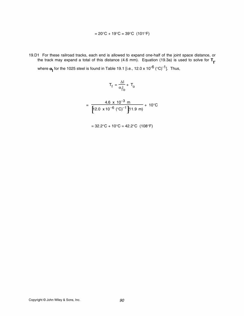
Copyright © John Wiley & Sons, Inc. 90
= 20°C + 19°C = 39°C (101°F)
19.D1 For these railroad tracks, each end is allowed to expand one-half of the joint space distance, orthe track may expand a total of this distance (4.6 mm). Equation (19.3a) is used to solve for T
f,
where ααααl for the 1025 steel is found in Table 19.1 [i.e., 12.0 x 10⁻⁶ (°C)-1]. Thus,
Tf =∆ l
αllo
+ To
= 4.6 x 10⁻³ m
12.0 x 10⁻⁶ (°C)−1[ ](11.9 m)+ 10°C
= 32.2°C + 10°C = 42.2°C (108°F)
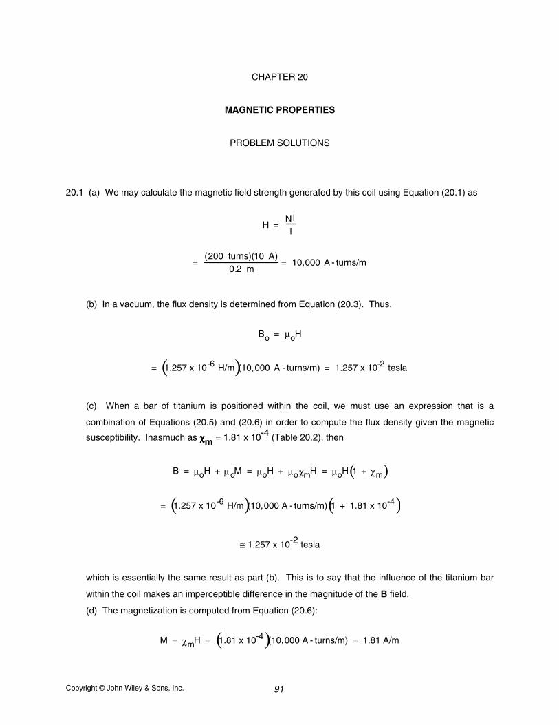
Copyright © John Wiley & Sons, Inc. 91
CHAPTER 20
MAGNETIC PROPERTIES
PROBLEM SOLUTIONS
20.1 (a) We may calculate the magnetic field strength generated by this coil using Equation (20.1) as
H =
N I
l
= (200 turns)(10 A)
0.2 m= 10,000 A - turns/m
(b) In a vacuum, the flux density is determined from Equation (20.3). Thus,
Bo = µoH
= 1.257 x 10⁻⁶ H/m( )(10,000 A - turns/m) = 1.257 x 10⁻² tesla
(c) When a bar of titanium is positioned within the coil, we must use an expression that is a
combination of Equations (20.5) and (20.6) in order to compute the flux density given the magnetic
susceptibility. Inasmuch as χχχχm = 1.81 x 10⁻⁴ (Table 20.2), then
B = µoH + µoM = µoH + µoχmH = µoH 1 + χm( )
= 1.257 x 10⁻⁶ H/m( )(10,000 A - turns/m) 1 + 1.81 x 10⁻⁴( )
≅ 1.257 x 10⁻² tesla
which is essentially the same result as part (b). This is to say that the influence of the titanium bar
within the coil makes an imperceptible difference in the magnitude of the B field.
(d) The magnetization is computed from Equation (20.6):
M = χmH = 1.81 x 10⁻⁴( )(10,000 A - turns/m) = 1.81 A/m
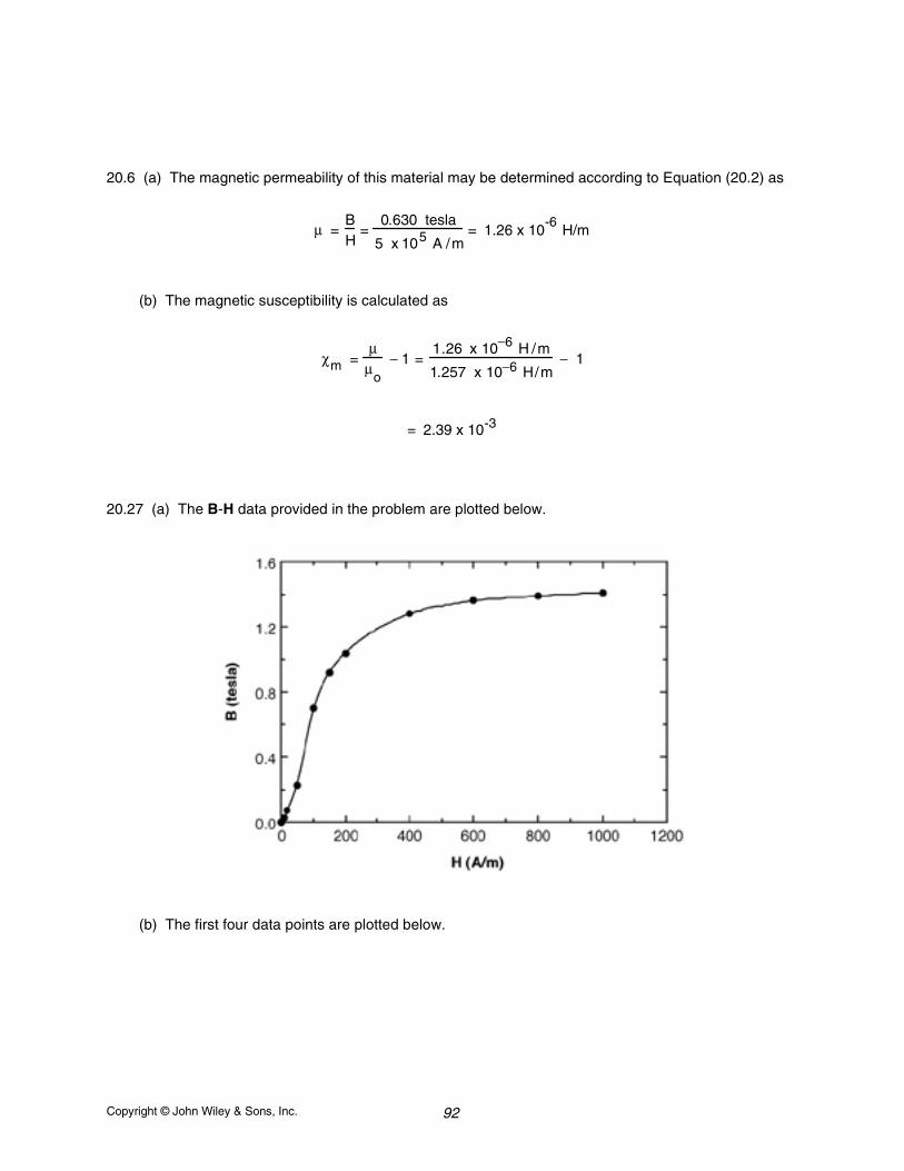
Copyright © John Wiley & Sons, Inc. 92
20.6 (a) The magnetic permeability of this material may be determined according to Equation (20.2) as
µ =BH
=0.630 tesla
5 x 10⁵ A /m= 1.26 x 10
-6 H/m
(b) The magnetic susceptibility is calculated as
χm =µ
µo
− 1 =1.26 x 10⁻⁶ H /m
1.257 x 10⁻⁶ H/m− 1
= 2.39 x 10⁻³
20.27 (a) The B-H data provided in the problem are plotted below.
(b) The first four data points are plotted below.
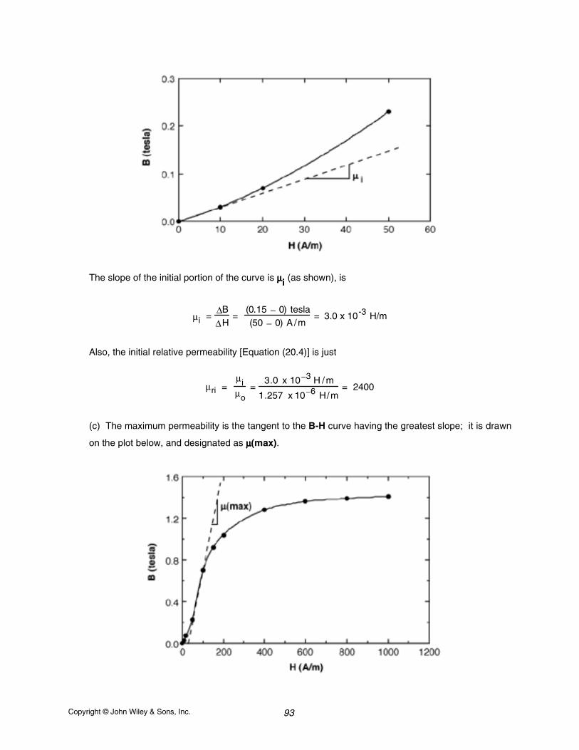
Copyright © John Wiley & Sons, Inc. 93
The slope of the initial portion of the curve is µµµµi (as shown), is
µi =∆B
∆H=
(0.15 − 0) tesla(50 − 0) A /m
= 3.0 x 10⁻³ H/m
Also, the initial relative permeability [Equation (20.4)] is just
µri = µiµo
=3.0 x 10⁻³ H /m
1.257 x 10⁻⁶ H/m= 2400
(c) The maximum permeability is the tangent to the B-H curve having the greatest slope; it is drawn
on the plot below, and designated as µµµµ(max).

Copyright © John Wiley & Sons, Inc. 94
The value of µµµµ(max) is
µ(max) =∆B∆H
= (1.3 − 0.3) tesla(160 − 45) A - m
= 8.70 x 10 -3
H/m
20.32 (a) Given Equation (20.12) and the data in Table 20.7, we are asked to calculate the criticalmagnetic fields for lead at 2.5 and 5.0 K. From the table, for Pb, TC = 7.19 K and BC(0) = 0.0803
tesla. Thus, from Equation (20.3)
HC(0) =BC(0)
µo
= 0.0803 tesla
1.257 x 10⁻⁶ H /m= 6.39 x 10⁴ A/m
Now, solving for HC(2.5) using Equation (20.12) yields
HC(T) = HC(0) 1 −T2
TC2
HC(2.5) = 6.39 x 10⁴ A /m( )1 −(2.5 K)2
(7.19 K)2
= 5.62 x 10⁴ A/m
(b) Now we are to determine the temperature to which mercury must be cooled in a magnetic field of15,000 A/m in order for it to be superconductive. The value of HC(0) must first be determined using
BC(0) given in the table (i.e., 0.0411 tesla); thus from Equation (20.3)
HC(0) =BC(0)
µo
=0.0411 tesla
1.257 x 10⁻⁶ H/m= 3.27 x 10⁴ A/m
Since TC = 4.15 K we may solve for T using Equation (20.12) as
T = TC 1 −HC(T)
HC
(0)
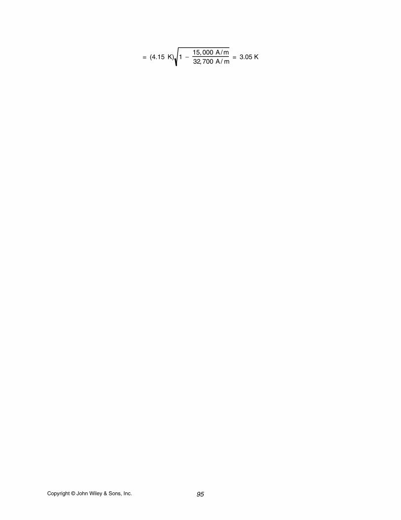
Copyright © John Wiley & Sons, Inc. 95
= (4.15 K) 1 −15,000 A/m32,700 A/ m
= 3.05 K
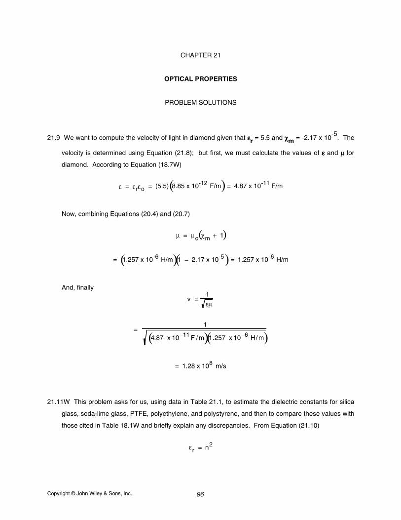
Copyright © John Wiley & Sons, Inc. 96
CHAPTER 21
OPTICAL PROPERTIES
PROBLEM SOLUTIONS
21.9 We want to compute the velocity of light in diamond given that εεεεr = 5.5 and χχχχm = -2.17 x 10⁻⁵
. The
velocity is determined using Equation (21.8); but first, we must calculate the values of εεεε and µµµµ for
diamond. According to Equation (18.7W)
ε = εrεo = (5.5) 8.85 x 10⁻¹² F/m( ) = 4.87 x 10⁻¹¹ F/m
Now, combining Equations (20.4) and (20.7)
µ = µo χm + 1( )
= 1.257 x 10⁻⁶ H/m( )1 − 2.17 x 10⁻⁵( ) = 1.257 x 10⁻⁶ H/m
And, finally
v =1
εµ
= 1
4.87 x 10⁻¹¹ F /m( )1.257 x 10⁻⁶ H/m( )
= 1.28 x 10⁸ m/s
21.11W This problem asks for us, using data in Table 21.1, to estimate the dielectric constants for silica
glass, soda-lime glass, PTFE, polyethylene, and polystyrene, and then to compare these values with
those cited in Table 18.1W and briefly explain any discrepancies. From Equation (21.10)
εr = n2
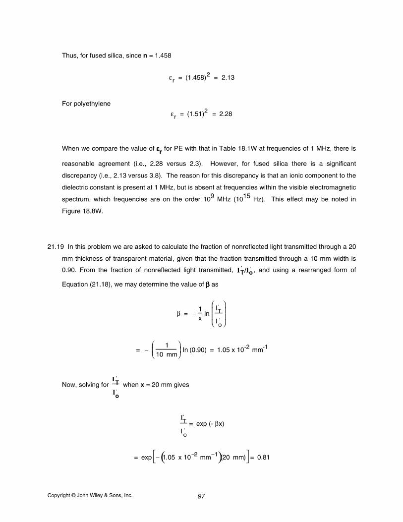
Copyright © John Wiley & Sons, Inc. 97
Thus, for fused silica, since n = 1.458
εr = (1.458)2 = 2.13
For polyethylene
εr = (1.51)2 = 2.28
When we compare the value of εεεεr for PE with that in Table 18.1W at frequencies of 1 MHz, there is
reasonable agreement (i.e., 2.28 versus 2.3). However, for fused silica there is a significant
discrepancy (i.e., 2.13 versus 3.8). The reason for this discrepancy is that an ionic component to the
dielectric constant is present at 1 MHz, but is absent at frequencies within the visible electromagnetic
spectrum, which frequencies are on the order 109 MHz (1015 Hz). This effect may be noted in
Figure 18.8W.
21.19 In this problem we are asked to calculate the fraction of nonreflected light transmitted through a 20
mm thickness of transparent material, given that the fraction transmitted through a 10 mm width is
0.90. From the fraction of nonreflected light transmitted, IT' /Io
' , and using a rearranged form of
Equation (21.18), we may determine the value of ββββ as
β = −1x
lnIT
'
Io'
= − 1
10 mm
ln (0.90) = 1.05 x 10⁻² mm-1
Now, solving for IT
'
Io'
when x = 20 mm gives
IT'
Io'
= exp (- βx)
= exp − 1.05 x 10⁻² mm−1( )(20 mm)
= 0.81
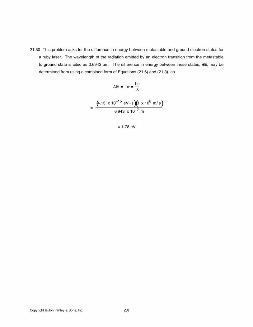
Copyright © John Wiley & Sons, Inc. 98
21.30 This problem asks for the difference in energy between metastable and ground electron states for
a ruby laser. The wavelength of the radiation emitted by an electron transition from the metastable
to ground state is cited as 0.6943 µm. The difference in energy between these states, ∆∆∆∆E, may be
determined from using a combined form of Equations (21.6) and (21.3), as
∆E = hν =hcλ
= 4.13 x 10⁻¹⁵ eV - s( )3 x 10⁸ m/ s( )
6.943 x 10⁻⁷ m
= 1.78 eV