Embed Size (px)
Citation preview
Math 145a Lecture Notes
Evan [email protected]
Harvard CollegeFall 2014
This is Harvard College’s Math 145a, instructed by Peter Koellner. Theformal name for this class is “Set Theory I”.
The permanent URL is http://web.evanchen.cc/coursework.html, alongwith all my other course notes.
Contents
1 September 2, 2014 51.1 Broad Overview . . . . . . . . . . . . . . . . . . . . . . . . . . . . . . . . 51.2 Introduction to Independence . . . . . . . . . . . . . . . . . . . . . . . . . 51.3 Example of Independence . . . . . . . . . . . . . . . . . . . . . . . . . . . 51.4 More Surprising Examples . . . . . . . . . . . . . . . . . . . . . . . . . . . 61.5 Escaping . . . . . . . . . . . . . . . . . . . . . . . . . . . . . . . . . . . . 71.6 Models and Compactness . . . . . . . . . . . . . . . . . . . . . . . . . . . 71.7 Looking Ahead . . . . . . . . . . . . . . . . . . . . . . . . . . . . . . . . . 71.8 So what happens in this class? . . . . . . . . . . . . . . . . . . . . . . . . 8
2 September 4, 2014 92.1 Sets . . . . . . . . . . . . . . . . . . . . . . . . . . . . . . . . . . . . . . . 92.2 Subsets . . . . . . . . . . . . . . . . . . . . . . . . . . . . . . . . . . . . . 92.3 Cantor’s Theorem . . . . . . . . . . . . . . . . . . . . . . . . . . . . . . . 92.4 Informal comprehension principle . . . . . . . . . . . . . . . . . . . . . . . 102.5 Empty set . . . . . . . . . . . . . . . . . . . . . . . . . . . . . . . . . . . . 112.6 Well-Orderings . . . . . . . . . . . . . . . . . . . . . . . . . . . . . . . . . 112.7 Ordinals . . . . . . . . . . . . . . . . . . . . . . . . . . . . . . . . . . . . . 122.8 The Hierarchy . . . . . . . . . . . . . . . . . . . . . . . . . . . . . . . . . 12
3 September 9, 2014 133.1 Housekeeping . . . . . . . . . . . . . . . . . . . . . . . . . . . . . . . . . . 133.2 Last Time . . . . . . . . . . . . . . . . . . . . . . . . . . . . . . . . . . . . 133.3 Quasi-philosophical interlude . . . . . . . . . . . . . . . . . . . . . . . . . 133.4 Categoricity . . . . . . . . . . . . . . . . . . . . . . . . . . . . . . . . . . . 143.5 Language of Set Theory . . . . . . . . . . . . . . . . . . . . . . . . . . . . 143.6 The First Five Axioms . . . . . . . . . . . . . . . . . . . . . . . . . . . . . 143.7 The Sixth Axiom, Infinity . . . . . . . . . . . . . . . . . . . . . . . . . . . 153.8 The Seventh Axiom, Foundation . . . . . . . . . . . . . . . . . . . . . . . 163.9 The Last Infinitely Many Axioms, Replacement . . . . . . . . . . . . . . . 16
1
Evan [email protected] (Harvard CollegeFall 2014)
Contents
4 September 11, 2014 174.1 Defining the nonnegative integers . . . . . . . . . . . . . . . . . . . . . . . 174.2 Comprehension and Collection . . . . . . . . . . . . . . . . . . . . . . . . 174.3 Set abstraction and the “set of all sets” . . . . . . . . . . . . . . . . . . . 174.4 Some abuse of notation with sets and classes . . . . . . . . . . . . . . . . 184.5 Some more basic notions . . . . . . . . . . . . . . . . . . . . . . . . . . . . 19
4.5.1 Intersection and Difference . . . . . . . . . . . . . . . . . . . . . . . 194.5.2 Ordered Pairs . . . . . . . . . . . . . . . . . . . . . . . . . . . . . . 194.5.3 Products . . . . . . . . . . . . . . . . . . . . . . . . . . . . . . . . . 194.5.4 Relations . . . . . . . . . . . . . . . . . . . . . . . . . . . . . . . . . 194.5.5 Functions . . . . . . . . . . . . . . . . . . . . . . . . . . . . . . . . . 20
4.6 Philosophy . . . . . . . . . . . . . . . . . . . . . . . . . . . . . . . . . . . 204.7 Axiom of Choice . . . . . . . . . . . . . . . . . . . . . . . . . . . . . . . . 20
5 September 16, 2014 215.1 Motivation . . . . . . . . . . . . . . . . . . . . . . . . . . . . . . . . . . . 215.2 Setup . . . . . . . . . . . . . . . . . . . . . . . . . . . . . . . . . . . . . . 215.3 Transfinite Induction . . . . . . . . . . . . . . . . . . . . . . . . . . . . . . 225.4 Transfinite Recursion . . . . . . . . . . . . . . . . . . . . . . . . . . . . . 225.5 Transfinite things can be BIG . . . . . . . . . . . . . . . . . . . . . . . . . 23
6 September 18, 2014 256.1 What does a well-ordering look like? . . . . . . . . . . . . . . . . . . . . . 256.2 Well-orderings look roughly the same . . . . . . . . . . . . . . . . . . . . 256.3 Stuff with classes . . . . . . . . . . . . . . . . . . . . . . . . . . . . . . . . 266.4 How to preserve transitive sets . . . . . . . . . . . . . . . . . . . . . . . . 276.5 Ordinals . . . . . . . . . . . . . . . . . . . . . . . . . . . . . . . . . . . . . 27
7 September 23, 2014 297.1 Recap . . . . . . . . . . . . . . . . . . . . . . . . . . . . . . . . . . . . . . 297.2 Order Types . . . . . . . . . . . . . . . . . . . . . . . . . . . . . . . . . . 297.3 Arithmetic on Ordinals . . . . . . . . . . . . . . . . . . . . . . . . . . . . 30
7.3.1 Addition . . . . . . . . . . . . . . . . . . . . . . . . . . . . . . . . . 307.3.2 Multiplication . . . . . . . . . . . . . . . . . . . . . . . . . . . . . . 307.3.3 Exponentiation . . . . . . . . . . . . . . . . . . . . . . . . . . . . . . 317.3.4 A nontrivial theorem . . . . . . . . . . . . . . . . . . . . . . . . . . 31
7.4 The hierarchy of sets, done with ordinals . . . . . . . . . . . . . . . . . . 317.5 The ordinals grab all the sets . . . . . . . . . . . . . . . . . . . . . . . . . 32
8 September 25 338.1 Axiom of Choice is equivalent to WO . . . . . . . . . . . . . . . . . . . . 338.2 Zorn’s Lemma . . . . . . . . . . . . . . . . . . . . . . . . . . . . . . . . . 338.3 Some weakenings of AC . . . . . . . . . . . . . . . . . . . . . . . . . . . . 34
9 September 30, 2014 359.1 Equinumerous sets . . . . . . . . . . . . . . . . . . . . . . . . . . . . . . . 359.2 Creating cardinals . . . . . . . . . . . . . . . . . . . . . . . . . . . . . . . 369.3 Properties of cardinals . . . . . . . . . . . . . . . . . . . . . . . . . . . . . 369.4 Recurse . . . . . . . . . . . . . . . . . . . . . . . . . . . . . . . . . . . . . 37
2
Evan [email protected] (Harvard CollegeFall 2014)
Contents
10 October 2, 2014 3810.1 Cardinal arithmetic . . . . . . . . . . . . . . . . . . . . . . . . . . . . . . 3810.2 Finite sets . . . . . . . . . . . . . . . . . . . . . . . . . . . . . . . . . . . . 3810.3 Infinite cardinal arithmetic is boring . . . . . . . . . . . . . . . . . . . . . 3910.4 Cardinal exponentiation . . . . . . . . . . . . . . . . . . . . . . . . . . . . 3910.5 Fundamental theorems of cardinal arithmetic . . . . . . . . . . . . . . . . 4010.6 Some exponentiation is not interesting . . . . . . . . . . . . . . . . . . . . 40
11 October 7, 2014 4111.1 Cofinality . . . . . . . . . . . . . . . . . . . . . . . . . . . . . . . . . . . . 4111.2 Lemmas on cofinality . . . . . . . . . . . . . . . . . . . . . . . . . . . . . 4111.3 Given AC, cofinalities and successor cardinals are regular . . . . . . . . . 4211.4 Inaccessible cardinals . . . . . . . . . . . . . . . . . . . . . . . . . . . . . 44
12 October 9, 2014 4512.1 Linear Orders . . . . . . . . . . . . . . . . . . . . . . . . . . . . . . . . . . 4512.2 Intermission . . . . . . . . . . . . . . . . . . . . . . . . . . . . . . . . . . . 4612.3 Separable complete linear orders . . . . . . . . . . . . . . . . . . . . . . . 4612.4 Suslin property . . . . . . . . . . . . . . . . . . . . . . . . . . . . . . . . . 47
13 October 14, 2014 4913.1 Sparse Review . . . . . . . . . . . . . . . . . . . . . . . . . . . . . . . . . 49
14 October 16, 2014 5014.1 Partitions . . . . . . . . . . . . . . . . . . . . . . . . . . . . . . . . . . . . 5014.2 Infinite Ramsey Theorem . . . . . . . . . . . . . . . . . . . . . . . . . . . 5014.3 Some negative results on partitions . . . . . . . . . . . . . . . . . . . . . . 5114.4 Large Cardinals . . . . . . . . . . . . . . . . . . . . . . . . . . . . . . . . 5214.5 Trees . . . . . . . . . . . . . . . . . . . . . . . . . . . . . . . . . . . . . . 53
15 October 21, 2014 5415.1 Definability . . . . . . . . . . . . . . . . . . . . . . . . . . . . . . . . . . . 5415.2 Fragments of the Universe . . . . . . . . . . . . . . . . . . . . . . . . . . . 5415.3 Definable sets . . . . . . . . . . . . . . . . . . . . . . . . . . . . . . . . . . 55
16 October 23, 2014 5716.1 Model theory notions . . . . . . . . . . . . . . . . . . . . . . . . . . . . . 5716.2 Reflection . . . . . . . . . . . . . . . . . . . . . . . . . . . . . . . . . . . . 5816.3 Variations . . . . . . . . . . . . . . . . . . . . . . . . . . . . . . . . . . . . 59
17 October 28, 2014 60
18 October 30, 2014 6118.1 Completing the proof of a theorem . . . . . . . . . . . . . . . . . . . . . . 6118.2 The statement Lκ V = L . . . . . . . . . . . . . . . . . . . . . . . . . . 6118.3 A Nice application of Reflection . . . . . . . . . . . . . . . . . . . . . . . 6318.4 A sketch of the proof that Lκ AC . . . . . . . . . . . . . . . . . . . . . 63
19 November 4, 2014 6419.1 Axiom of Choice . . . . . . . . . . . . . . . . . . . . . . . . . . . . . . . . 6419.2 GCH . . . . . . . . . . . . . . . . . . . . . . . . . . . . . . . . . . . . . . . 6419.3 Hulls . . . . . . . . . . . . . . . . . . . . . . . . . . . . . . . . . . . . . . . 65
3
Evan [email protected] (Harvard CollegeFall 2014)
Contents
19.4 Summary . . . . . . . . . . . . . . . . . . . . . . . . . . . . . . . . . . . . 66
20 November 6, 2014 6720.1 β-Gaps . . . . . . . . . . . . . . . . . . . . . . . . . . . . . . . . . . . . . 6720.2 A Taste of Fine Structure . . . . . . . . . . . . . . . . . . . . . . . . . . . 6720.3 The Guessing Sequence . . . . . . . . . . . . . . . . . . . . . . . . . . . . 68
21 November 11, 2014 7021.1 Problems with trying to set up Forcing . . . . . . . . . . . . . . . . . . . 7021.2 Coding; good and bad reals . . . . . . . . . . . . . . . . . . . . . . . . . . 7121.3 Ground Models . . . . . . . . . . . . . . . . . . . . . . . . . . . . . . . . . 71
22 November 13, 2014 7222.1 The generic extension M [G] . . . . . . . . . . . . . . . . . . . . . . . . . . 7222.2 Existence of generic extensions . . . . . . . . . . . . . . . . . . . . . . . . 7222.3 Splitting posets . . . . . . . . . . . . . . . . . . . . . . . . . . . . . . . . . 7322.4 Defining the generic extension . . . . . . . . . . . . . . . . . . . . . . . . 7322.5 Defining M [G] . . . . . . . . . . . . . . . . . . . . . . . . . . . . . . . . . 74
23 November 18, 2014 7523.1 Review of Names . . . . . . . . . . . . . . . . . . . . . . . . . . . . . . . . 7523.2 Filters of Transitive Models . . . . . . . . . . . . . . . . . . . . . . . . . . 7523.3 Using the Generic Condition . . . . . . . . . . . . . . . . . . . . . . . . . 77
24 November 20, 2014 7824.1 Motivation . . . . . . . . . . . . . . . . . . . . . . . . . . . . . . . . . . . 7824.2 Semantics and Desired Conditions . . . . . . . . . . . . . . . . . . . . . . 7824.3 Defining the Relation . . . . . . . . . . . . . . . . . . . . . . . . . . . . . 7924.4 Consequences of the Definition . . . . . . . . . . . . . . . . . . . . . . . . 80
25 December 2, 2014 8125.1 Forcing tells us that M [G] satisfies ZF . . . . . . . . . . . . . . . . . . . . 8125.2 Forcing V 6= L is really easy . . . . . . . . . . . . . . . . . . . . . . . . . . 8225.3 Forcing ZFC + ¬CH . . . . . . . . . . . . . . . . . . . . . . . . . . . . . . 83
26 December 4, 2014 8426.1 The Countable Chain Condition . . . . . . . . . . . . . . . . . . . . . . . 8426.2 Possible Values Argument . . . . . . . . . . . . . . . . . . . . . . . . . . . 8426.3 Preserving Cardinals . . . . . . . . . . . . . . . . . . . . . . . . . . . . . . 8526.4 Infinite Combinatorics . . . . . . . . . . . . . . . . . . . . . . . . . . . . . 8626.5 Finishing Off . . . . . . . . . . . . . . . . . . . . . . . . . . . . . . . . . . 8626.6 Concluding Remark . . . . . . . . . . . . . . . . . . . . . . . . . . . . . . 87
4
Evan [email protected] (Harvard CollegeFall 2014)
1 September 2, 2014
§1 September 2, 2014
§1.1 Broad Overview
The text for this course is Set Theory, by Koellner, which I just downloaded. Thegrading for this course is 100% problem sets.
The course has three parts,
• an introduction to set theory,
• the constructible universe,
• the Solovay model and forcing.
The goal of the course is the second and third part, in which we prove some things areindependent. For example, CH is independent of ZFC.1
Today we’ll be talking about the notion of independence.
§1.2 Introduction to Independence
This is “chapter 0”, not yet in the text.There are, very broadly, two kinds of mathematics.
1. Algebraic, which is not in general concerned with a specific structure. For example,group theory or theory of rings, topology, and so on. These topics are not aboutspecific structures like N.
2. In contrast, non-algebraic stuff is concerned with a specific structure. For example,number theory cares a lot about N. (In a bit, we will show that (N, 0, S,+×),where S is a successor function, is unique up to isomorphism.) As another example,analysis, which cares about (PN,∈). Note that 2N ∼ R. As a third example,functional analysis cares about (PPN,∈).
Set theory is the second type, and we care about iterating P . Iterating n times gives Vn.
• Vn is finite combinatorics.
• Vω ∼ N
• Vω+1 ∼ PN.
§1.3 Example of Independence
Take the axioms of group theory: given (G, ·) we require
(1) ∀x, y, xy ∈ G
(2) ∀x, y, z we have x(yz) = (xy)z
(3) ∃1 ∈ G: ∀x, x · 1 = 1 = 1 · x
(4) ∀x ∈ G, ∃y ∈ G with xy = 1 = yx.
Consider (5), G is abelian (meaning xy = yx)
1Axioms of infinity makes certain things more answerable. ZFC “can’t articulate large enough objects”.We can introduce larger and larger infinities, much like a “name the larger number” game that smallchildren play.
5
Evan [email protected] (Harvard CollegeFall 2014)
1 September 2, 2014
Fact. The “abelian” statement is independent of the group axioms (1) through (4).
Proof. There exist both abelian (Z) and non-abelian (D6) groups. Duh.
So this is not a big deal in algebra, because there are tons of groups, and no one wastrying to determine whether “THE group” was abelian.
On the other hand, independence in Euclidean geometry might be a bit more surprising– we now know the parallel postulate is independent of the other four of Euclid’s axioms.2
That’s because we’re talking about ONE THING. Of course now we have like non-Euclidean geometry, and geometry as a formal discipline became just like group theory.
So once we discovered the parallel postulate was independent of the other four, geometryfractured into “formal” geometry and “applied” geometry.
Philosophical question now: do we have independence with “fixed” structures?
§1.4 More Surprising Examples
Let’s take number theory! This has a fixed structure, (N, 0, S).The axioms of this structure are denoted PA, the Peano axioms. This again has five
axioms.
(1) 0 is a number.
(2) If x is a number, so is S(x).
(3) S(x) 6= 0 for any x.
(4) S(x) = S(y) =⇒ x = y.
(5) (Least Criminal) If 0 has property ϕ (denoted ϕ(0)), and ∀x : ϕ(x) =⇒ ϕ(Sx),then ϕ(x) holds for all x.
The last axiom is the one that’s doing all the work – ∞ is packaged in the first fouraxioms.
Again, the principle is that the resulting structure is FIXED. In the “second order”form of the axioms, PA determines N up to isomorphism. So there “should” not beundecidable things!
Question 1.1. Is PA complete?3 In other words, is it the case that for any sentence ϕ(in the language of PA) that either PA ` ϕ or PA ` ¬ϕ?
Here PA ` ϕ means PA proves ϕ.So the answer is Godel’s incompleteness theorems – no.
Theorem 1.2 (Godel’s First Incompleteness Theorem)
Assume that PA is consistent. Then there exists a ϕ such that PA can neither proveϕ nor ¬ϕ.
Remark. Godel had to assume a tiny bit more. The above statement is Rosser’s version.
2Note that Euclid’s axioms suck. There are twenty-one Tarski axioms.3Tarski’s geometry is complete – there is only “one” Euclidean geometry.
6
Evan [email protected] (Harvard CollegeFall 2014)
1 September 2, 2014
Theorem 1.3 (Godel’s Second Incompletness Theorem)
Assume PA is consistent. Then PA cannot prove its own consistency.
One can express “PA is consistent” in the language of Peano arithmetic. This is a lot likethe “liar” paradox: namely “this sentence is false”. Similarly, we construct a statement“I’m not provable”.
This is like bad. Outside of PA we can see the truth of PA, but not from within itself.
§1.5 Escaping
It’s not enough to add Con(PA) to the system. Godel’s Theorem generalizes as fol-lows.
Theorem 1.4
For any extension T of PA, T cannot prove Con(T ).
§1.6 Models and Compactness
Theorem 1.5 (Godel, Compactness)
Suppose T is a formal system such that every finite fragment of T has a model.Then T has a model (i.e. it is consistent).
Consider the following: let us add a constant symbol c to the language of PA. Let T bethe following list of axioms:
• PA
• c 6= 0
• c 6= 1
• c 6= 2
• . . .
Obviously every finite fragment of T has a model. So T has a model! Let’s call thismodel
(M, 0, S, c).
The axioms of Peano arithmetic implies we have S(c), S(S(c)). That means there are“strange” numbers in addition to this chain of fake numbers hanging out on the side.
§1.7 Looking Ahead
For set theory,we have a system, ZFC. By Godel, we know if ZFC is consistent, thenZFC cannot prove its own consistency.
However, we can find worse examples.
Question 1.6 (Continuum Hypothesis). Is there an infinite subset A ⊂ R such thatA 6∼ N and A 6∼ R?
7
Evan [email protected] (Harvard CollegeFall 2014)
1 September 2, 2014
Theorem 1.7 (Godel, 1938)
If ZFC is consistent, then ZFC cannot refute CH.
Theorem 1.8 (Cohen, 1965)
If ZFC is consistent, then ZFC cannot prove CH.
This is really terrible because CH does not refer to the system of axioms at all (unlikeCon(PA) or Con(ZFC)).
We also have the following fact.
Fact 1.9. Up to isomorphism, (R, <) is the unique dense linear ordering without endpointsthat is separable (i.e. has a countable dense subset).
Hint: it’s Q.
Remark. Separable implies every disjoint sequence of intervals is countable.
Question 1.10 (Suslin’s Hypothesis). Is the above theorem still true if we replace “sepa-rable” with the weaker condition that “every disjoint sequence of intervals is countable”?
This is again independent of ZFC.These two questions are pretty unfortunate because this time, we have picked the
question “before” the choice of axioms (namely ZFC).
§1.8 So what happens in this class?
1. Part 1 of the course will talk about ZFC.
2. Part 2 of the course (“the constructible universe”) will deal with Godel’s proof thatZFC cannot refute CH.
3. Part 3 of the course (“forcing”) will deal with Cohen’s proof that ZFC cannot proveCH.
8
Evan [email protected] (Harvard CollegeFall 2014)
2 September 4, 2014
§2 September 4, 2014
This class is pretty flexible. Anyways, here is an informal introduction to the notions ofset theory.
§2.1 Sets
First we contrast sets and concepts. Examples of concepts are:
• “is red” – applies to red things
• “is a human being”
• “is a featherless biped”
These concepts apply to various things. By the way, the two latter things apply to thesame thing, Homo Sapiens. However, they are different concepts.
Sets do NOT have this feature.
Adam,Eve, . . . = featherless bipeds .
Hence given the set, we cannot tell what concept created it. In other words:
Sets are determined by their elements, while concepts are not determined bythe things falling under them.
Remark 2.1. Sets are extensional, which means
A = B iff ∀x (x ∈ A ⇐⇒ x ∈ B) .
This is the formalization of the above notion.
§2.2 Subsets
Consider N = 0, 1, 2, 3, . . . , . We can consider subsets – write
A ⊂ B iff ∀x (x ∈ A =⇒ x ∈ B) .
Let E = 0, 2, 4, . . . ⊂ N and O = 1, 3, 5, . . . ⊂ N. Note that E ∩O = ∅ = .The key operation is considering all subsets. Consider all subsets N, including E and
O. Notice that E and O are definable. Unfortunately there are only countably manydefinable sets (while 2N ∼ R is uncountable). However, we are still interested in theundefinable sets.
PutP(N) = A : A ⊆ N
as the power set of N. (Here P(X) is defined analogously.)
§2.3 Cantor’s Theorem
Some useful notions (er, more like review):
• Given f : A→ B, we say f is onto or surjective if f(A) = B.
• Moreover, f is one-to-one injective if it never collapses elements; ∀x, y ∈ A (x 6= y =⇒ fx 6= fy).
• Finally, f is bijective if f is both one-to-one and onto.
9
Evan [email protected] (Harvard CollegeFall 2014)
2 September 4, 2014
Definition 2.2. Two sets A and B have the same size if and only if ∃f : A→ B whichis one-to-one and onto.
This lifts this criterion up to infinite sets. If you leave a knife and fork for each personat a table (possibly infinitely large) then there are the same number of knives andforks.
Example 2.3
As above, E ∼ N ∼ O. Also, Q ∼ N.
Theorem 2.4 (Cantor)
N 6∼ R.
Proof. Hmm this is a new one. Assume for contradiction we can enumerate the reals asx1, . . . .
Consider the following sequence of nested closed intervals. Start with I0 = [0, 1]. LetI1 = [a1, b1] be such that b1 − a1 ≤ 1
1 and x1 /∈ [a1, b1]. Then set I2 = [a2, b2] ⊆ I1 withb2 − a2 ≤ 1
2 and x2 /∈ I2. Continue.This gives rise to a nested sequence of intervals
I0 ⊃ I1 ⊃ . . . .
By design, xn /∈ In for any n. However these intervals are all closed, so⋂n≥0 In = x
for some x. Hence this x is not of the form xk, contradiction.
This generalizes as follows.
Theorem 2.5
For any set X, P(X) 6∼ X.
Proof. Barber paradox. Also on our Math 55 pset.
Now that the review is done, let’s state some philosophy.
The idea of P(X) is one of the two key ideas of set theory.
Now what’s the second idea?
§2.4 Informal comprehension principle
The informal comprehension principle states the following: if X is a set and P as adefinite4 property of elements in X, then there exists a set Y which contains all and onlythe elements P holds for. In other words,
Y = x ∈ X : P (x)
is a set. Another name is the “informal separation principle”.
4An example of non-definite property is “is bald”. The hallmark of a vague property is that it doesn’tobey induction. If a person with n hairs is bald, is someone with n+ 1 hairs bold?
10
Evan [email protected] (Harvard CollegeFall 2014)
2 September 4, 2014
Example 2.6
Take X = N. Then D is even.
Remark 2.7. Note that this does NOT imply that all sets are generated by compre-hension. Indeed, if there are only countably many properties, so some subsets of N arenecessarily not generated by properties.
§2.5 Empty set
Definition 2.8. Define ∅ = x : x 6= x.
The empty set has the very important property that it is a subset of everything.We could have started with N. Specifically,
• N is where all number theory happens.
• P(N) ∼ R is where all algebra happens.
• P(P(N)) ∼ f : R→ R is where all algebra happens.
But we start lower. We have
V1 = P(∅) = ∅ = V2 = P(P(∅)) = ∅, ∅
V3 = P(P(P(∅))) = ∅, ∅ , ∅ , ∅, ∅ .
Notice that in general, the nth iteration is a power tower of 2’s:
∣∣P5(∅)∣∣ = 222
2
= 216 = 65536.
These numbers get quite big quite quickly.Let’s give these things a name.
Definition 2.9. Let V0 = ∅ and Vn+1 = P(Vn).
Despite how large these numbers are, the collection of Vnn is pretty countable. Define
Vω =⋃
n<ω
Vn.
Then N ∼ Vω, R ∼ Vω+1, and we recover our ladder.Note that Cantor’s Continuum Hypothesis is that there are no cardinalities between|Vω| and |Vω+1|.
§2.6 Well-Orderings
Definition 2.10. Suppose ≺ is a binary relation (whatever that means) on a set X.Then ≺ is well-founded if and only if every non-empty subset Y of X has an ≺-minimalelement. Moreover, ≺ is well-ordered if it is well-founded, strict, linear.
Example 2.11
The relation “is an ancestor of” on humans is well-founded. Similarly, < is well-founded on N. However, > is not well-founded over N.
11
Evan [email protected] (Harvard CollegeFall 2014)
2 September 4, 2014
§2.7 Ordinals
Are there larger examples?Let ω be the next ordinal after all the nonnegative integers. If we want to be formal,
ω = 0, 1, 2, 3, . . . . We can then posit ω + 1, and keep going. Thus we have
0 < 1 < 2 < · · · < ω < ω + 1 < . . .
Another similar vein is re-ordering the integers as
0 < 2 < 4 < 6 < · · · < 1 < 3 < 5 < . . .
which is certainly a valid ordering. These have the same order type – there is an obviousorder-preserving bijection between them. Thus we focus on the former, which are calledthe ordinals.
Exercise. Check that these are well ordered! It’s an finite way down, but possibly aninfinite way up.
Let’s start talking about ordinals (keeping in mind everything up to now is stillinformal).
0,1, 2, 3, . . . , ω
ω + 1, ω + 2, . . . , ω + ω
2ω + 1, 2ω + 2, . . . , 3ω
...
ω2 + 1, ω2 + 2, . . .
...
ω3, . . . , ω4, . . . , ωω
...,
Here I’m abusing notation. The notion 2ω should be ω + ω; the notion ω2 should beω · ω, but you get the idea.
We finish with ωω...
here ω many times, which is called ε0. In general, εk+1 is εk stackedk times. Then we get to εε0 , and so on. . .
Remark 2.12. Compute ωε0 = ε0. Actually, ε0 is the least α such that ωα = α.
Transfinite induction with ε0
§2.8 The Hierarchy
Let V be the universe of sets. Iterate P along all the well-orderings.Later we’ll see the following:
• V0 = ∅
• Vα+1 = P(Vα) (successor)
• Vλ =⋃α<λ Vα if λ is a limit
• V =⋃α∈On Vα.
Here On is the order types of everything. We’ll show soon On 6⊂ On and V /∈ V .
12
Evan [email protected] (Harvard CollegeFall 2014)
3 September 9, 2014
§3 September 9, 2014
§3.1 Housekeeping
• Office hours: Tuesday 2PM - 3PM, 414 2 Arrow Street
• Book: A Course in Set Theory, by Ernest S
• Email professor: background (logic, ST, math) and what you would like to see
Exercises coming next week.
§3.2 Last Time
Subject matter: set theory hierarchy.Three fundamental ideas:
• Well-ordering (ordinals)
• Power set
• Absolute infinity, which we’ll discuss more below.
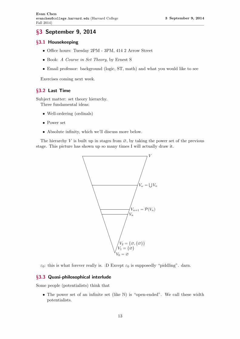
The hierarchy V is built up in stages from ∅, by taking the power set of the previousstage. This picture has shown up so many times I will actually draw it.
V
V0 = ∅
Vω =⋃Vn
Vn+1 = P(Vn)Vn
V1 = ∅V2 = ∅, ∅
ε0: this is what forever really is. :D Except ε0 is supposedly “piddling”. darn.
§3.3 Quasi-philosophical interlude
Some people (potentialists) think that
• The power set of an infinite set (like N) is “open-ended”. We call these widthpotentialists.
13
Evan [email protected] (Harvard CollegeFall 2014)
3 September 9, 2014
• The height of the universe (ordinals) is “open-ended”. We call these height poten-tialists.
Why would someone think 2N is open-ended? We showed that |P(N)| > |N| already.Some people think the idea P(N) does not even make sense. The potentialists thinkthat subsets of N which are definable make sense but are skeptical of the notion of “all”subsets of N.
Consider a binary branching tree which represents decisions on whether to include anelement of N. (Going right at the nth step means including n in.)
Anyways the opposite of a potentialist is an actualist.
§3.4 Categoricity
We now show the philosophy is a moot point. Suppose we have two hierarchies V0, V1, . . .and V ′0 , V
′1 , . . . . Since N is isomorphic in these things, there as an isomorphism of Vω to
V ′ω. Now in my senseVω+1 = P V (Vω) .
In your senseV ′ω+1 = P V
′ (V ′ω).
But any A specified in Vω leads to a set of V ′ω.OK I have no idea what this is. But it was informal. The point is going to be
categoricity. Regardless of what makes sense and what does not, apparently everythingis isomorphic?
§3.5 Language of Set Theory
OK whatever, let’s consider the universe V .In number theory, we defined the integers through a successor function. The analog
here is the power set operator P.We now enter the domain of Chapter 1, the language of set theory. Firstly it ni the
language of logic. This includes ∀, ∃, an infinite supply of variables, as well as negation¬, ∧, ∨, and finally → and ↔. Moreover, we have a symbol =.
You can’t say too much with this; in Number Theory we solve this problem by defininga few extra things, 0 and the successor function S, among other things. In set theory weadd only one symbol: the membership ∈. For example, consider
∀x∃y(x ∈ y).
This has important implications: we can already generate N by
x ∈ y0 ∈ y1 ∈ y2 ∈ . . .
Now we can prepare the axioms.
§3.6 The First Five Axioms
First, we distinguish a set from a concept.
Axiom I (Extensionality). A set is determined by its elements, meaning
∀x∀y∀z ((z ∈ x↔ z ∈ y)→ x = y) .
Now we need to begin somewhere.
14
Evan [email protected] (Harvard CollegeFall 2014)
3 September 9, 2014
Axiom II (Empty Set). The empty set exists: ∃x∀y(y /∈ x).
By Extensionality, there is only one such empty set, and we denote it by ∅.
Axiom III (Pairing). Informally, for any x, y we can create x, y. Formally,
∀x∀y∃a∀z (z ∈ a↔ (z = x ∨ z = y)) .
Again by Extensionality, this set is unique, and we denote it by x, y.
Axiom IV (Union). Informally, we can take⋃a′∈a. Formally,
∀x∃a∀z (z ∈ a↔ ∃y (z ∈ y ∈ x)) .
Again by Extensionality (see a pattern here?), this is unique, so we call it⋃x.
Example 3.1
If x = N, ⋃x = N. So that means using union, we can generate large sets fromsmall ones.
Now for the power set.
Axiom V (Power Set). We can construct P(x). Formally,
∀x∃a∀y(y ∈ a↔ y ⊆ x)
where y ⊆ x is short for ∀z(z ∈ y → z ∈ x).
Again, we do not have a lot of symbols, so we define lots of shorthands like ⊆. Theimportant thing is that this in principle can be expanded. Anyways, we denote this byP(x) since it is unique by Extensionality.
§3.7 The Sixth Axiom, Infinity
Note that the first five axioms are already sufficient to construct
P(P(. . . (∅))).
This lets us get up to the natural numbers.Moreover, remark that Vω =
⋃n∈N Vn is a model for these axioms. Just check all the
axioms hold.But Vω is countable, and all the sets are freaking finite. Boring! Let’s force infinitely
large sets.
Axiom VI (Infinity).
∃x (∅ ∈ x ∧ ∀y (y ∈ x→ y ∪ y ∈ x)) .
This time we can’t conclude x is unique. But we can deduce some things:
∅ ∈ x =⇒ ∅ ∈ x=⇒ ∅, ∅ ∈ x=⇒ ∅, ∅ , ∅, ∅ ∈ x. . .
15
Evan [email protected] (Harvard CollegeFall 2014)
3 September 9, 2014
Actually, each line is just the union of the objects on all the previous lines. This is a lotlike ω, where we define ω = 0, 1, 2, . . . , and ω + 1 = 0, 1, 2, . . . , ω. Basically, the waywe generate a new object is to take the set of all previous objects.
Anyways, x is not unique. We can throw in ∅ in or something, and suddenly weget more junk in x. However, there is nonetheless a minimal x. Here’s how we get ourhands on it: Call a set x inductive if
∅ ∈ x ∧ ∀y (y ∈ x→ y ∪ y ∈ x) .
Then define ω =⋂A | A inductive. (We’ll define
⋂later).
§3.8 The Seventh Axiom, Foundation
Now we will make induction work by ruling out infinite chains.
Axiom VII (Foundation).
∀x (x 6= ∅→ ∃y ∈ x∀z ∈ x(z /∈ y)) .
Equivalently, “there are no infinite descending ∈ chains”.
This is not too hard to see. Suppose
x1 3 x2 3 x3 3 . . .
Then take x = xkk≥1, which fails Foundation. Conversely, if Foundation fails then it isnot hard to generate an infinite 3 chain.
Anyways, what is a model for this? If we take the universe Vω+1 = PVω, it turns outthat this satisfies Infinity, because Vω ∈ Vω+1. However, it doesn’t satisfy Power Setanymore, because P(Vω+1) is not in there. Nonetheless, we can extend this up to Vω+ω,and now we have a model!
You might ask why we don’t just stop at Vω+ω. Mainly, because we can. Like, FLTwas not proved in ZFC. If you give yourself more machinery, you can prove more stuff.
§3.9 The Last Infinitely Many Axioms, Replacement
ZFC does not have eight axioms, it has infinitely many! We just like to condense this asreplacement.
Axiom VIII (Replacement). For each formula ϕ in the Language of Set Theory, andfor every positive integer n,
∀p1∀p2 . . . ∀pn∀a [∀y ∈ a ∃!z ϕ(y, z, p1, p2, . . . , pn)]
→ [∃b ∀z (z ∈ b↔ ∃y ∈ a ϕ (y, z, p1, . . . , pn))] .
What is this saying? Really ϕ defines a function F (relative to the parameters pi) ondomain a, then we can collect them together in a set b = F (a).
It turns out the Replacement does not hold in Vω+ω because there is no set
Vω, Vω+1, Vω+2 . . . .
Actually, Replacement blows the top off this, making ε0 seem small. Oops.
16
Evan [email protected] (Harvard CollegeFall 2014)
4 September 11, 2014
§4 September 11, 2014
Happy 18th birthday, Jessica!In what follows, we will just abbreviate ϕ(x, p1, . . . , pn) as ϕ(x).
§4.1 Defining the nonnegative integers
Last time we introduced ZF and the language of set theory.First, let us actually define
0 = ∅1 = ∅2 = ∅, ∅3 = ∅, ∅ , ∅, ∅
and in general, n+ 1 = 0, 1, . . . , n. Then ω =⋃n∈N n.
§4.2 Comprehension and Collection
Here are two more schemes, not part of ZFC.
Axiom (Comprehension). For any ϕ in LST,
∀a∃b∀x (x ∈ b↔ x ∈ a ∧ ϕ(x)) .
Very loosely, this states that you can do something like
x ∈ A | ϕ(x)
Axiom (Collection). For any ϕ in LST,
∀a [∀y ∈ a∃!zϕ(y, z)]→ ∃b∀y ∈ ∃z ∈ bϕ(y, z)
In other words, if ϕ defines a “function”.Collection is “looser” than replacement. Given a set A, replacement states that it’s
possible to get f(A) exactly, “replacing” every element of a ∈ A with f(a). Collectiononly lets you collect them in a big blob.
Exercise 4.1. In ZF without replacement, Comprehension and Collection together areequivalent to replacement.
Sketch of Proof. It’s easy to see Comprehension and Collection together give Replacement.Also, Replacement implies Collection. To see Replacement gives Comprehension, assumeB 6= ∅ and contrive a function.
§4.3 Set abstraction and the “set of all sets”
Because Comprehension holds in ZF, we can write the shorthand
x ∈ a | ϕ(x) .
This is called a set abstract The condition x ∈ a is crucial; it must be a restricted abstract.Otherwise everything burns.
What happens when this restriction is dropped? The resulting expression may thenfail to denote a set.
17
Evan [email protected] (Harvard CollegeFall 2014)
4 September 11, 2014
Proposition 4.2
The expression x | x = x is not a set.
Proof. Assume not, and let v denote it. Clearly v = v, so v ∈ v. Then
v ∈ v ∈ v ∈ . . .
which breaks Foundation.
In other words, the universe V = x | x = x is not itself a set.The way to think of this is that “I am in this room” is not the same as “this room is
contained in the physical universe”. The universe is not really a container; it is a “stage”on which the actual sets lie.
Nonetheless, we will use this notation for non-sets as well. Just be careful. . . In theabove, V is not a set, it is a class. But for example, consider the expression
z | ∃y (z ∈ y ∧ y ∈ a) .
This is a set by replacement; roughly, consider a function x 7→ x. To write it as arestricted comprehension, we must use
z ∈ P(a) | ∃y (z ∈ y ∧ y ∈ a) .
§4.4 Some abuse of notation with sets and classes
Despite the warning above, we will write
b ∈ x | ϕ(x)
which doesn’t necessarily make sense, since the RHS is not really a set, but this isshorthand for ϕ(b). (Note we can’t replace ∈ with 3 here!)
Similarly, we may writex | ϕ(x) = x | ψ(x)
as shorthand for∀x (ϕ(x)↔ ψ(x)) .
Similarly,x | ϕ(x) ⊆ x | ψ(x)
is shorthand for∀x (ϕ(x)→ ψ(x)) .
Just distinguish with sets and classes. . .That means we can write the following shorthands.
• Comprehension states that for all sets x and classes C, C ∩ x is a set.
• Replacement states that For all sets a and all class functions F , the image F (a)is a set.
• Collection is similar to replacement but only gives you that F (a) is a subset ofsome set.
18
Evan [email protected] (Harvard CollegeFall 2014)
4 September 11, 2014
§4.5 Some more basic notions
4.5.1 Intersection and Difference
Definition 4.3 (Intersection). Given x, we define the intersection by
⋃x = z | ∀y ∈ x(z ∈ y) .
This is a set because we can put z ∈ ⋃ y.
Definition 4.4 (Difference). Given x and y, define the difference by
x \ y = z ∈ x | z /∈ y .
4.5.2 Ordered Pairs
We would like to define ordered pairs as well; x1, x2 = x2, x1 so we need a newnotion.
Definition 4.5. Let (x1, x2) denote x1, x1, x2.
Notice that (x1, x2) 6= (x2, x1) if x1 6= x2, and (x, x) = x , x, x = x , x =x.
Exercise 4.6. Show that (x1, x2) = (y1, y2) if and only if x1 = y1 and x2 = y2.
4.5.3 Products
We can define the direct product.
Definition 4.7. Define
X × Y = (x, y) | x ∈ X ∧ y ∈ Y .
We claim this is a set. Just notice we can carve it out from⋃P(P(X ∪ Y )).
Naturally, we can also define
X1 ×X2 × · · · ×Xn+1 = (X1 × · · · ×Xn)×Xn+1.
We also write Xn = X ×X × · · · ×X.
4.5.4 Relations
An n-ary relation R on a class X is a subclass of Xn.Suppose n = 2. The domain of R is
dom(R) = x ∈ X | ∃y(x R y) .
Similarly,the range isran(R) = y ∈ Y | ∃x(x R y) .
Then we letfield(R) = dom(R) ∪ ran(R).
We can defineR−1 = (y, x) | (x, y) ∈ R .
Finally, we say that R is
19
Evan [email protected] (Harvard CollegeFall 2014)
4 September 11, 2014
• reflexive if ∀x ∈ X, x R x..
• symmetric if ∀x, y ∈ X, x R y → y R x.
• transitive if ∀x, y, z ∈ X we have x R y ∧ y R z → x R z.
It is an equivalence relation if all three are true. This gives us a partition into equivalenceclasses [a]R.
Exercise 4.8. Show that
(i) X =⋃ [a]R | x ∈ X.
(ii) ∀a, b ∈ X (¬ (a R b)→ [a]R ∩ [b]R = ∅)
4.5.5 Functions
A function is a binary relation R such that
∀x ∈ dom(R) ∃!y ∈ ran(R) : x R y.
We’ll use f and g, thanks. Also, for sets X and Y write
XY = f | f : X → Y .
Thus ωω is the functions from N to N. We sometimes abuse notation if there is nopossibility of confusion and write this as Y X .
Restriction, images, inverses.
§4.6 Philosophy
Everything is a set. N is a set. R = P(N) is a set. And so on.OK let’s move on.
§4.7 Axiom of Choice
Axiom IX (Choice). We have
∀x (∀y ∈ x (y 6= ∅))→ ∃f (f is a function, dom(f) = x, ∀y ∈ x (fy ∈ y)) .
In other words, given a bunch of nonempty sets x = y1, y2, . . . , we can construct achoice function f with f(yi) ∈ yi for all i.
Note that this can be proven in the case x is finite. Let x = y1, where y1 6= ∅. Lookat all functions f with domain x and f(y1) ∈ y1.
In the case x = y1, y2 with y1, y2 6= ∅.Then y1 × y2 6= ∅.In other words, Choice states that y1 × y2 × . . . is nonempty, even in the infinite case.
Exercise 4.9. Show that Choice is equivalent to
∀x∀y∀f : x→ y ∃(g : ran(f)→ x) such that g ⊆ f−1.
20
Evan [email protected] (Harvard CollegeFall 2014)
5 September 16, 2014
§5 September 16, 2014
Summary so far:
(1) informal introduction to the subject matter of set theory
• V
• two fundamental notions: well-ordering (stages) and power sets (what we doto stages)
(2) axioms of set theory
Now, we redo our (1) formally using (2).Recall (informally) our ordinals, 0, . . . , ε0, . . . . We’re going to make this all rigorous
now.
§5.1 Motivation
Our motivation is that we are going to try and generalize the natural numbers ω. Recallwe have induction: if ϕ(0) and ∀n (ϕ(n)→ ϕ(n+ 1)) then ∀nϕ(n). This is not enoughto get up to ω. Now we’re going to generalize this massively a la “strong induction”.
We are also going to generalize recursion. Given a point p, if we can get f(p) from allpredecessors of p, then we have a recursion.
We’re going to do this vastly more generally, on well-founded rather than just well-ordered relations.
§5.2 Setup
Let R be a binary relation on X.
Definition 5.1. We say R is strict or irreflexive if ∀x ∈ X, x R x does NOT hold. Wesay R is linear if ∀x, y ∈ X either x R y or y R x.
Then for each x ∈ X, let
extR(x) = y ∈ X | y R x .
Example 5.2
Let R denote “is a parent of” and X be the set of humans. Then R is strict but notlinear. Moreover, extR(x) are the parents of x.
Definition 5.3. The transitive closure TC(R) is the intersection of all transitiverelations containing R.
By taking the intersection of them all, we get rid of the “junk” and get the smallestpossible.
Example 5.4
TC(“is a parent of ”) = “is an ancestor of”.
Definition 5.5. The predecessors are predR(x) = extTC(R)(x). A subset Y of X isR-transitive if for all y ∈ Y , predR(y) ⊆ Y .
21
Evan [email protected] (Harvard CollegeFall 2014)
5 September 16, 2014
Example 5.6
The set predR(Fred Koellner) ∪ predR(Obama) is R-transitive.
Definition 5.7. An element y ∈ Y is R-minimal if there is no z ∈ Y such that z 6= yand z R y.
Then a relation R (on X, even if it is a class rather than a set) is well-founded if
(i) Every nonempty subset Y has an R-minimal element
(ii) ∀x ∈ X, extR(x) is a set.
Note that this last relation is obvious for X a set. However, we can consider X a class aswell, so long as locally everything looks like a set (for example, “set of all sets”).
Definition 5.8. A well-ordering is a well-founded, strict, linear relation.
§5.3 Transfinite Induction
Now we can generalize induction and recursion to well-founded relations. (If you look atthe proof of induction, neither “linear” nor “countable” is needed.)
Theorem 5.9 (Transfinite Induction)
Suppose R is a well-founded relation on X. If Y ⊆ X is such that
∀x ∈ X (predR(x) ⊆ Y → x ∈ Y )
then Y = X.
In other words, let Y be some subset of X. Suppose that any time the predecessors of xare in Y , then x is in Y too. It follows that, actually, all of X is in Y .
The “base cases” are handled by predR(x) = ∅ for any R-minimal element x.
Proof. Suppose that Y 6= X and consider X − Y . Then let a be an R-minimal elementin X − Y . Now all the guys in predR(a) cannot be in X − Y , so they are contained in Y .Contradiction.
§5.4 Transfinite Recursion
Likewise, we can also build objects on well-founded structures.
Theorem 5.10 (Transfinite Recursion)
Suppose R is a well-founded relation on X. Suppose
G : X × V → V
is a class function. Then there’s a unique function
F : X → V
so that for all x ∈ X,F (x) = G(x, F |predR(x)).
Here F |predR(x) is a restriction.
22
Evan [email protected] (Harvard CollegeFall 2014)
5 September 16, 2014
Here G is a “generating function” in the sense of the recursion. Our G takes in an x andthe predecessors, and spits out F (x). Intuitively, G has way, way more information thanwe need.
Proof. First, we show uniqueness. Suppose F1 and F2 are two distinct such functions.Use transfinite induction to show they are equal: consider the R-minimal point a withF1(a) 6= F2(a). Then F1|predR(a) = F2|predR(a), contradicting that G is a function.
For existence, take an R-minimal element x. Our G gives G(x,∅), so now we knowF (x). Intuitively, it’s clear how to proceed.
Let us say a function f : D → V is good if
(i) D ⊆ X and ∀x ∈ D(predR(x) ⊆ D)
(ii) ∀x ∈ D we have f(x) = G(x, f |pred(x)).
In other words, f is doing the right thing on a predecessor-closed subset of X.First, suppose f1 : D1 → V and f2 : D2 → V . We claim f1|D1∩D2 = f2|D1∩d2 . The
proof is exactly the same as that for uniqueness.The second claim is that ⋃
dom(P ) | f is good
is X. Now suppose f : predR(x)→ V is good for some x. Define f ′ : predR(x)∪x → Vby
y 7→f(y) if y ∈ predR(x)
G(x, f) otherwise.
This is clearly good. So we have shown that
predR(x) ⊆⋃dom(f) | f is good → x ∈
⋃dom(f) | f is good .
The second claim then follows by transfinite induction.Finally, let F =
⋃ f | f good. By Claim 1 this is a function. By Claim 2, dom(F ) =X. Hence F is good.
§5.5 Transfinite things can be BIG
Let G : V × V → V , and let R be the membership relation ∈. For any set x, we have
ext∈(x) = x.
Then pred∈(x) consists of a very nested sequence of things. In particular, ∅ ∈ pred∈(x).It really goes ALL THE WAY DOWN.
A second example is
G : On× V → V by (α, f) 7→P (⋃
ran(f)) if α 6= ∅∅ otherwise.
with R as <. The transitive recursion gives us an F such that for any α ∈ On we have
F (α) = G(α, Fα)
and you can check that in fact,
F (0) = F (∅) = G(∅,∅) = ∅ = V0.
23
Evan [email protected] (Harvard CollegeFall 2014)
5 September 16, 2014
Oops okay this doesn’t actually work. OK, the correct version is
G : On× V → V by (α, f) 7→
∅ if α = ∅P(⋃
ran(x)) if α is a successor⋃ran(x) if α is a limit.
24
Evan [email protected] (Harvard CollegeFall 2014)
6 September 18, 2014
§6 September 18, 2014
Last time we looked at transfinite induction as well-founded relations.Basically, a well-founded relation (X,R) is just one step shy of being a sub-chunk of
the ordinals. A well-founded relation looks a lot like a poset with a base. You can haveinfinite ascending sequences, just not descending ones (limit points).
A special case is a well-orderings. The main topic for today.
§6.1 What does a well-ordering look like?
Imagine a poset with a base in which every two things are comparable. Oh wait, we havea total order.
We can also add limit points.Anyways, the basic claim is that any well-ordering is just isomorphic to sub-orderings
of the standard ordering of the ordinals.
§6.2 Well-orderings look roughly the same
Definition 6.1. Suppose (X,R) is a well-ordering. For x ∈ X, we define anotherwell-ordering
IRx =(predR(x), R ∩ predR(x)2
).
Here IRx and R itself are called the initial segments of (R,X).
Intuitively, all we’re doing is cutting off our relation past x.
Remark. A different notation of a well-ordering is (A,<A). We sometimes also abbreviate(X,R) as just R.
The following proof is just a generalization of the proof that the natural numbersare unique up to isomorphism. First, let us make sure we agree on the definition ofisomorphism:
Definition 6.2. Suppose (X,R) and (X ′, R′) are well-orderings. We say that (X,R) ∼=(X ′, R′) are isomorphic if f is bijective.
Remark. We can weaken “bijective” to “surjective” because R′ is strict and R is linear.Explicitly, if x1 6= x2, then they are R-related, so fx1 and fx2 are R-related and hencenot equal.
Theorem 6.3
Suppose (X,R) and (Y, S) are well-orderings. Then either
(i) R ∼= ISy for some y ∈ Y ,
(ii) IRx∼= S for some x ∈ X,
(iii) R ∼= S.
Again, the proof is just to walk upwards.
25
Evan [email protected] (Harvard CollegeFall 2014)
6 September 18, 2014
Proof. For A ⊆ X, f : A→ Y and x ∈ X. We use transfinite recursion. Let
G(x, f) =
s-least element in Y − f(predR(x)) if possible
undefined otherwise..
OK this is pretty sloppy. But lol. We’re allowed to be sloppy because in set theory,functions are just pairs, and so “undefined” means we just don’t add a pair. Butconsequently, G might not have the full domain X.
But the point is that if we exhaust S, then we’re done, and if we haven’t run out ofthings in S, we just keep going.
Let F be defined by transfinite recursion from G. By transfinite induction we have
∀x ∈ dom(F )F (predR(x)) = predS (F (x)) .
Also it’s easy to see F is order-preserving (both ways). Blah.OK we finish by considering three cases.
(1) If dom(F ) = X and ran(F ) = Y , then R ∼= S.
(2) If dom(F ) = X and ran(F ) 6= Y , then just take the minimal element y of Y −ran(F ),then this must be equal to predS(y), thus R ∼= ISy .
(3) The case dom(F ) 6= X is handle similarly and we obtain R ∼= IRx .
§6.3 Stuff with classes
For a given well-ordering (X,R) consider the class of all well-orderings (X1, R′) suchthat
(X ′, R′) ∼= (X,R).
This gives a massive equivalence class.
Example 6.4
The equivalence class of (ω,∈) has a lot of things. For example, consider (Even, <),(Odd, <). This is not even a set. Given S, we can construct a copy of ω by putting∈ on
S, S, S, . . .and things blow up!
Also the equivalence classes are stacked too. For C1 and C2 are equivalence classes ofa well-ordering. Pick (x1, R1) ∈ C1 or (X2, R2) ∈ C2. WLOG, assume R1 is an initialsegment of R2. Then every guy in C1 is an initial segment of C2. That means theequivalence classes are well-ordered too.
Now we want to pick a specific canonical representative from each equivalence class.Here’s how you do it. Given (X,R) a representative of a class, we want to add a singleelement. There are tons of elements not in X, but the canonical one is X. Hence we do
X ′ = X ∪ X
andR′ = R ∪ (y,X) | y ∈ X .
So starting with the empty set, we have a trivial relation (∅,∅), and we recover theordinals.
26
Evan [email protected] (Harvard CollegeFall 2014)
6 September 18, 2014
§6.4 How to preserve transitive sets
Recall that a set A is transitive if a ∈ A =⇒ a ⊆ A.
Lemma 6.5
If X is transitive then
(a) X ∪ X is transitive
(b) ∪X is transitive
(c) P(X) is transitive.
Proof. (a) Consider x ∈ X and do cases on x ∈ X versus x = X.
(b) Suppose X is transitive. Then ∪X is transitive. Suppose a ∈ ∪X. Then a ∈ b ∈ Xfor some b. By transitivity, a ∈ X, and hence by union a ⊆ ∪X.
(c) Check it.
Of course, ∅ is transitive. So Vα are all transitive by invoking the lemma. The stemOn consists of transitive sets too.
§6.5 Ordinals
Definition 6.6. An ordinal is a transitive set that is well-ordered by ∈.
Let On denote the class of ordinals.Every transitive set is closed under membership ∈. Ordinals are additionally well-
ordered under ∈.You can show that any transitive well-ordering is isomorphic to some ordinal.
Exercise 6.7. If α ∈ On and β ∈ α then β ∈ On.
Proof. To show β is transitive, use both the fact that α is transitive and well-ordered.(Neither alone is sufficient.)
To show that β is well-ordered by ∈, then. . .
Exercise 6.8. If α ∈ On thenα = β | β < α .
Here < means ∈.
Lemma 6.9
Suppose α ∈ β ∈ On. The following are equivalent. Then α ∈ β if and only if α ( β.
Proof. Clearly α ∈ β =⇒ α ⊆ β, and α 6= β is not possible (since otherwise β ∈ β).The reverse is more tricky.
Now suppose α ( β. Since β is well-ordered under membership, we can consideran ∈-least element b in β − α. By the first exercise, b ∈ On. By the second exercise,b = γ | γ < b = α. So α ∈ β.
27
Evan [email protected] (Harvard CollegeFall 2014)
6 September 18, 2014
Theorem 6.10 (Linearity)
If α and β are ordinals then either α ≤ β or β ≤ α.
Proof. Check α ∩ β ∈ On. We claim that α ∩ β is either α or β. If not, α ∩ β ( α, β. Bythe lemma, α∩β ∈ α and α∩β ∈ β. Hence α∩β ∈ α∩β and that is a contradiction.
Theorem 6.11
On is not a set.
Proof. Assume Ω is the set of all ordinals. Then Ω is well-ordered by ∈. Moreover, ifa ∈ b ∈ Ω, then b is an ordinal, so a is on ordinal, hence Ω is transitive.
28
Evan [email protected] (Harvard CollegeFall 2014)
7 September 23, 2014
§7 September 23, 2014
§7.1 Recap
• Well-orderings and well-founded relations
• Transfinite induction
• Transfinite reduction
• Well-ordering theorems – isomorphism.
• On is not an ordinal (not a set)
Recall that an ordinal is a transitive set which is well-ordered by the relation ∈.
§7.2 Order Types
We will now show that ordinals are indeed a canonical representative.
Theorem 7.1 (Comprehensiveness)
Fro every well-ordering (X,R) there is an ordinal α such that
(X,R) ∼= (α,∈).
This proof is a little subtle. Actually, Schimmerling does not give a full proof.
Proof. Fix a well-ordering (X,R).
Claim. For any a ∈ X there is a unique ordinal α with IRa∼= (α,∈).
Proof of lemma. First, we prove existence. Take the R-minimal one a ∈ X. Then lookat the things below it:
∀a ∈ X(aRa→ ∃!x ∈ On IRa ∼= (α,∈)
).
Now pick using Replacement
α =α | ∃aRa IRa ∼= (α,∈)
.
To prove α is an ordinal, it suffices to prove that it is is transitive (since it is clearlywell-ordered by ∈). You can check this. Fix α ∈ α ∈ α. Then α has an a ∈ IRa ∼= (α,∈).Now α ∈ (α,∈), so a ∈ IRa . That gives α ∈ α.
Hence there exists such an α with
IRa∼= (α,∈) .
Of course, this α is unique, since
(α,∈) ∼= IRa∼=(α′,∈
)
implies α ∼= α′.
Hence, for any initial segment in (X,R) we can get a corresponding ordinal. Now tohit all of (X,R) we can set
β =β | ∃a ∈ XIRa ∼= (β,∈)
.
29
Evan [email protected] (Harvard CollegeFall 2014)
7 September 23, 2014
Definition 7.2. Suppose (X,R) is a well-ordering. Then the order type of (X,R) is theunique ordinal α such that (X,R) ∼= (α,∈).
Exercise 7.3. Show that there are arbitrarily large limit ordinals.
This is not true without Replacement, since Vω+ω is a model of ZFC minus Replacement.You need Replacement to show that λ+ ω is a set for any limit ordinal λ.
§7.3 Arithmetic on Ordinals
There are two approaches,
• transfinite induction,
• explicit construction.
We want to get α+ β, α · β, αβ.
7.3.1 Addition
The transfinite recursion method is as follows.
α+ 0 = α
α+ (β + 1) = (α+ β) + 1
α+ λ =⋃
β<λ
(α+ β).
Here λ 6= 0.For explicit construction, we work by concatenation. Suppose we have (X,R), (Y, S)
(so we do this with any well-orderings rather than just with ordinals, even though it’sthe same concept.). Basically we want to stick Y on top of X, so we do a quick hack byusing ordered pairs. Define
(X,R) + (Y, S) = ((0 ×X) ∪ (1 × Y ) , <lex)
Yay. Since we can add well-orderings, we can add ordinals by just looking at order types.It is not too hard to check that these definitions coincide (just use transfinite induction).
Example 7.4
Note that 2014 + ω = ω 6= ω + 2014.
Remark 7.5. Ordinal addition is not commutative. However, it is associative.
7.3.2 Multiplication
Again, it suffices to define things using transfinite recursion.
α · 0 = α
α · (β + 1) = (α · β) + α
α · λ =⋃
β<λ
α · β.
We can also do explicit construction.
α · β = (β × α,<lex) .
Again transfinite induction lets you show these are the same.
30
Evan [email protected] (Harvard CollegeFall 2014)
7 September 23, 2014
Example 7.6
Check that 2014 · ω = ω 6= ω · 2014 for similar reasons as addition.
Remark 7.7. Like addition, multiplication is associative (since we just get orderedtriples in the second definition), but not commutative.
7.3.3 Exponentiation
The recursion is clear.
α0 = 1
αβ+1 = αβ · ααλ =
⋃
β<λ
αβ.
The explicit construction is more complicated here, so tl;dr, have fun with the exercises.
7.3.4 A nontrivial theorem
Exercise 7.8 (Division Algorithm). Suppose we have a “base” ordinal β > 0. Let α bean ordinal. Then there exists a unique choice of γ1, γ2 such that
α = β · γ1 + γ2
and γ2 < β.
Proof. Mimic the proof of the division algorithm.
Theorem 7.9 (Cantor Normal Form)
Suppose α > 0 is an ordinal. Then α can be written uniquely as
α = ωβ1 · κ1 + ωβ2 · κ2 + · · ·+ ωβn · κn
where α > β1 > · · · > βn ≥ 0 are ordinals, and κ1, . . . , κn, n are positive integers.
Proof. Transfinite induction. Just greedily do it. LOL.
§7.4 The hierarchy of sets, done with ordinals
Definition 7.10. By transfinite induction, we set
V0 = ∅Vα+1 = P(Vα)
Vλ =⋃
α<λ
Vα
Finally, let V be the following class.
V =⋃
α∈On
Vα.
This is the “cumulative hierarchy of sets”.
31
Evan [email protected] (Harvard CollegeFall 2014)
7 September 23, 2014
Lemma 7.11
For all α, β ∈ On such that α < β,
(1) Vα is transitive,
(2) Vα ⊆ Vβ.
Proof. The proof of (1) is just transfinite induction on α. For (ii), Vα ∈ Vβ =⇒ Vα ⊆ Vβ .(The first part is just mass power set.)
§7.5 The ordinals grab all the sets
Exercise 7.12. Show that
x | x = x = Vdef=
⋃
α∈On
Vα
In other words, every set is picked up in⋃α∈On(Vα).
Proof. If some set doesn’t appear, take an ∈-minimal set not in any ordinal (possiblesince Foundation tells us ∈ is well-founded). Thus the key is Foundation.
The exercise implies the following notion is well-defined.
Definition 7.13. The rank of a set x, written rank(x), is the least α such that x ∈ Vα+1.
Remark 7.14. Notice that rank(α) = α and rank(Vα) = α for every α ∈ On.
Here is an alternative definition.
Definition 7.15. Show that an equivalent definition is as follows. By transfinite recursionon (V,∈), we define for each x ∈ V with x 6= ∅ by
ρ(∅) = 0
ρ(x) =⋃
y∈x(ρ(y) + 1)
Remark 7.16. This is why we want to have transfinite recursion on well-foundedstructures, not just well-orderings.
Exercise 7.17. Show that rank and ρ coincide.
32
Evan [email protected] (Harvard CollegeFall 2014)
8 September 25
§8 September 25
Today we discuss cardinals. In ordinals, order matters; it doesn’t for cardinals. Note thatordinals and cardinals coincide in the finite case.
Ordinals are a canonical representative for well-orderings. The idea is to do the samething with equivalence classes of bijections: we want to pick a canonical representativefor each of these guys.
At the end of this lecture, we state CH and then shoot for it.
§8.1 Axiom of Choice is equivalent to WO
Recall that our axiom states that there exists a choice function for any collection of setsX.
Cantor implicitly assumes that every set can be well-ordered. (Can R be well-ordered?)This isn’t quite true.
Theorem 8.1 (Zermelo, 1904)
The following are equivalent.
(1) AC, the Axiom of Choice.
(2) WO, which states that every set X can be well-ordered.
Proof. First, let us show that AC implies WO. Let X be an arbitrary set. Pick a choicefunction f on P(X) − ∅ (this follows from AC). Hence every subset Y ⊆ X has achoice f(y) ∈ X.
First, pick x1 = f(X) ∈ X. Now we have a first element. Select x2 = f(X − x1) ∈X − x1, and so on. In general, we wish to define f∗ : β → X such that for each α < β,
f∗(α) = f(X)−⋃
x∈αf∗(x).
This process cannot continue forever, since otherwise X is bijected to the ordinals, whichis impossible (recall that X is a set). Hence we can find β as above, so we have awell-ordering of X, namely β.
Now assume WO; we wish to show AC. Let X be an arbitrary set whose elements arenot ∅. Now take a well-ordering R on
⋃X. Then given any set Y ∈ X, we just the
R-minimal element.
Yeah OK so AC is equivalent to the assertion that everything is well-ordered. GG.
§8.2 Zorn’s Lemma
Definition 8.2. Let (X,EX) be a poset or partial ordering; i.e. a reflexive transitiverelation on the set X An element of x ∈ X is maximal if
@x′ ∈ X(x / x′.
)
Definition 8.3. A subset C ⊆ X is a chain if C is linearly ordered by EX . An elementis x ∈ X is an upper bound for a chain C if ∀c ∈ C, c EX x.
Remark. Note that this upper bound does not nead to lie in C.
33
Evan [email protected] (Harvard CollegeFall 2014)
8 September 25
Definition 8.4 (Zorn’s Principle). If (X,≤X) is a partial ordering such that every chainhas an upper bound then (X,EX) has a maximal element.
Theorem 8.5 (Zorn’s Lemma)
AC is equivalent to Zorn’s Principle.
Proof. Assume AC and WO. We wish to show ZP. Let (X,EX) be a partial order suchthat all chains have an upper bound.
By WO we can put a well-order ≺ with order type β on X. Pick first the ≺-minimalpoint x0 = f(0). Then let x1 be the ≺-least point above x0. Repeat for the successors(we’re using our contradiction assumption). Then we’ll set xω to be the ≺-least z abovethe chain x0 / x1 / x2 / . . . . In general set xλ to be the ≺-least number above xα forevery α < λ. This process must terminate eventually, since the resulting chain C can beembedded in β. It can only terminate when we have reached a maximal element.
Now to show that ZP implies AC. Look at the set of partial choice functions P , orderedby EP be the poset of partial choice functions on X “ordered by extension”; i.e.
P =f : X →
⋃X is a choice function | X 6= ∅ and X ⊆ X
.
The order is just f EP g if and only if f ⊆ g (not dom f ⊆ dom g!). Observe that for anychain C, the function
⋃C is an upper bound for the chain C. By Zorn, we now have
a maximal element in P , denoted F . It follows that F is the required choice function,because the only possible maximal elements of F are complete choice functions.
Moral: partial orders should approximate the order that you wantReverse mathematics: our lemmas prove the axioms.
§8.3 Some weakenings of AC
Definition 8.6 (Dependent Choice, DC). Given a relation ∼ such that for every x thereis something related to it, we can construct a chain xi : i < ω such that for all i < w,we have
xi ∼ xi+1.
This is called “dependent” since previous steps matter for future steps.
Exercise 8.7. Show that AC implies DC.
Fact 8.8. DC does not imply AC.
Definition 8.9. A set X is countable if and only if X can be bijected to ω.
Definition 8.10 (Countable Choice, ACω). Every countable set of nonempty sets has achoice function.
Exercise 8.11. Show that DC implies ACω.
Fact 8.12. ACω does not imply DC.
34
Evan [email protected] (Harvard CollegeFall 2014)
9 September 30, 2014
§9 September 30, 2014
Last time we showed AC, WO, and Zorn are equivalent.In what follows, AC is not assumed until further notice.
§9.1 Equinumerous sets
The following definition is actually really important; historically, it was not recognized assignificant.
Definition 9.1. Two sets A and B are equinumerous, written A ≈ B, if there is abijection between them.
Definition 9.2. We say A B if we can injection A into B.
Clearly, N Q R, and N ≈ Q 6≈ R.
Example 9.3
Set E = 0, 2, 4, . . . and O = 1, 3, 5, . . . . Then E ≈ N ≈ O.
Example 9.4
N× N ≈ N.
The following fundamental theorem shows that this notation makes sense.
Theorem 9.5 (Cantor-Bernstein)
Suppose A B and B A. Then A ≈ B.
Proof. We are given injective functions f : A→ B and g : B → A and desire a bijectionh : A→ B.
Define X0 = A, Y0 = B, and recursively set
Xn+1 = g(Yn) and Yn+1 = f(Xn).
This gives us a set of chainsX0 ⊇ X1 ⊇ X2 ⊇ . . .
and similarly for Y . Let X∞ =⋂n∈NXn. Define now h : A→ B by
x 7→
f(x) if x ∈ Xn \Xn+1 for some even n
g−1(x) if x ∈ Xn \Xn+1 for some odd n
f(x) if x ∈ X∞.
The point is that f(X∞) = g−1(X∞) = Y∞, so in the last sentence we could replace fwith g−1 (this would lead to a different h, but both are still bijections).
Check that this works.
35
Evan [email protected] (Harvard CollegeFall 2014)
9 September 30, 2014
§9.2 Creating cardinals
Definition 9.6. A cardinal is an ordinal κ such that for no α < κ do we have α ≈ κ.
Remark 9.7. These are also called initial ordinals.
You can check that all the ordinals ω + ω, ω2, ωω, and even ε0 are all countable sets,so none of them are cardinals.
Remark 9.8. The first few cardinals are 0, 1, . . . . Then, ω is a cardinal as well, and weset ℵ0 = ω.
Our goal is to prove the following proposition.
Proposition 9.9
There are arbitrarily large cardinals.
If we had WO (equivalently AC) right now, for X we could define
|X| = least ordinal κ with X ≈ κ.
This must be a cardinal, by definition. (The existence of such a κ is equivalent to WO.In fact, AC is equivalent to every set having a cardinality.) Now we could construct acardinal greater than ω by taking |P(ω)|, which is a cardinal.
However, one can show this without WO.
Exercise 9.10. Given an ordinal κ, let κ+ be the least ordinal cardinal greater than κ.Show that κ+ exists.
Sketch. Take the supremum of all the guys that have a 1 − 1 correspondence with κ.Show that the guys form a set. Use Replacement?
This shows that the class of cardinals C is not a set. For otherwise, ∪C has a cardinalityκ, but there’s a cardinal greater than κ in C.
§9.3 Properties of cardinals
Lemma 9.11
Given any set A of cardinals,⋃A is a cardinal.
This can let us construct ℵω.
Proof. If A has a maximal element κ, then⋃A = κ and we’re done.
Now suppose there is no largest cardinal. Suppose for contradiction that ∃α < ⋃Awhich can be bijected to it by some function f . So let κ ∈ ⋃A be such that α < κ. Thenκ can be injected to α by restricting f , contradiction.
Corollary 9.12
ℵω exists.
Proof. Set A = ℵ0,ℵ1, . . . , and note that A is a set by Replacement. Now apply theabove lemma.
36
Evan [email protected] (Harvard CollegeFall 2014)
9 September 30, 2014
§9.4 Recurse
Summary: given a cardinal κ we can construct κ+ a “successor” cardinal, and given aset of cardinals A we have
⋃A is a cardinal.
Hence by transfinite recursion we can define the following.
Definition 9.13. For any α ∈ On, we may define
ℵ0 = ω
ℵα+1 = (ℵα)+
ℵλ =⋃
α<λ
ℵα.
Example 9.14
Here are some big ordinals.ℵω,ℵε0
andℵℵω ,ℵℵℵω , . . .
If we take this to the limit, we get a κ such that ℵκ = κ. This is called an “ℵ-fixedpoint”.
It’s interesting to note that looking at the first few cardinals ℵ0, ℵ1, . . . , it seems thatthe cardinal is much bigger than its index. Evidently, the κ mentioned above is the unionof ℵℵℵ... , where we have n ℵ’s.
Then we can take κ+, . . .So now we have even showed there are arbitrarily large ℵ-fixed points, say κ0, κ1, . . . .
Lemma 9.15
If κ is a cardinal then either κ is finite (i.e. κ ∈ ω) or κ = ℵα for some α ∈ On.
Proof. Assume κ is infinite. Take α minimal with ℵα ≥ κ. For contradiction supposeℵα > κ.
Now, consider two cases. If α is a limit ordinal λ, then ℵλ is the supremum⋃γ<λ ℵγ .
So some γ < λ has ℵγ > κ.On the other hand, suppose α = α+ 1. Then
ℵα < κ < ℵα
are three cardinals. This is a contradiction.
Remark 9.16. Still no AC!
The Continuum Hypothesis (CH) says that if X ⊂ P(ω) is infinite, then either X ≈ ωor X ≈ P(ω). Given AC, we can talk about |R|, in which case CH states |R| = ℵ1.
37
Evan [email protected] (Harvard CollegeFall 2014)
10 October 2, 2014
§10 October 2, 2014
More on cardinals.
§10.1 Cardinal arithmetic
Recall the way we set up ordinal arithmetic. Note that in particular, ω + ω > ω andω2 > ω.
But cardinals count cardinality. We want to have
ℵ0 + ℵ0 = ℵ0
ℵ0 × ℵ0 = ℵ0
because ω+ω and ω ·ω are countable. In the case of cardinals, we simply “ignore order”.The following definition uses the Axiom of Choice.
Definition 10.1. The cardinality |X| of a set X is the least ordinal α such that |X| ≈ α.
Recall that ≈ means “equinumerous”, and this is well-defined. (AC implies that Xhas a well-ordering, so there is at least one such ordinal).
Definition 10.2 (Cardinal Arithmetic). Given cardinals κ and λ, define
κ+ λ = |(0 × κ) ∪ (1 × λ)|
andk × λ = |λ× κ| .
§10.2 Finite sets
Definition 10.3. A set X is
• finite if |X| < ω.
• countable if |X| ≤ ω.
• uncountable if |X| > ω.
Here are two nice characterizations of finite-ness.
Definition 10.4. A set is Dedekind-finite (abbreviated D-finite) if every injectivefunction from X to itself is also surjective.
Exercise 10.5. Show that a set is finite if and only if it is Dedekind finite.
Definition 10.6. A set X is D∗-finite if there exists f : X → X such that for no subset∅ ( Y ( X is f closed under Y (meaning f(Y ) ⊆ Y ).
Exercise 10.7. Show that this is also a characterization of finite sets.
Partial Proof. Look at a, f(a), f2(a), . . .
and let this be Y . If Y is finite done. Otherwise take Y − a.
Without AC you can find models of set theory for which the above equivalences break.
38
Evan [email protected] (Harvard CollegeFall 2014)
10 October 2, 2014
§10.3 Infinite cardinal arithmetic is boring
For finite cardinals, we can show that
n×m > n+m > n,m.
But now we have the following property of cardinal arithmetic.
Theorem 10.8
Let κ be an infinite cardinal. Then κ× κ = κ.
Proof. By transfinite induction (which is fine because we are working over ordinals), wemay assume that the theorem holds for all infinite cardinals κ < κ. Put an orderingon κ × κ as follows: for (α, β) and (γ, δ) in κ × κ set (α, β) / (γ, δ) if and only ifmax(α, β) < max(γ, δ) or the maximums are equal and (α, β) <lex (γ, δ). (This gives a“diagonal” argument.)
We claim that the order type of (κ× κ, /) equals κ.Count the /-predecessors of some (α, β) ∈ κ× κ. We claim there are at most
|(max(α, β) + 1)× (max(α, β) + 1)|
such points. Set κ = |max(α, β) + 1| < κ. By induction, |κ× κ| = κ.Hence we’ve shown that there are at most κ points /-below any pair, which implies
that ot(κ× κ, /) = κ.
Corollary 10.9
Given cardinals κ and λ, one of which is infinite, we have
κ× λ = κ+ λ = max (κ, λ) .
Proof. Compute
max (κ, λ) ≤ κ+ λ
≤ κ× λ≤ max (κ, λ)×max (κ, λ)
= max (κ, λ) .
§10.4 Cardinal exponentiation
Unlike in addition and multiplication, we do not ignore order for exponentiation.
Definition 10.10. Suppose κ and λ are cardinals. Then
κλ = |F (λ, κ)| .
Here F (A,B) is the set of functions from A to B.
Example 10.11
2ℵ0 gives us binary numbers, R.
Continuum Hypothesis states that 2ℵ0 = ℵ1.
39
Evan [email protected] (Harvard CollegeFall 2014)
10 October 2, 2014
§10.5 Fundamental theorems of cardinal arithmetic
Theorem 10.12 (Cantor)
For all κ, κκ > κ.
Proof. We already have seen (from Cantor) that
2ℵα > ℵα
for every ordinals α. For all κ, since κκ = 2κ (why?), we have κκ > κ.
Theorem 10.13 (Konig)
For all finite κ, we have κcof(κ) > κ.
Here cof(κ) is cofinality, which we haven’t defined yet.We are going to show that these two theorems are “all we can prove” in ZFC.There are some trivial things we can prove, like
Lemma 10.14
We have(κλ)µ = κλ·µ.
Proof. This was like a Math 55 problem. Biject
F (µ,F (λ, κ))→ F (λ× µ, κ)
in the obvious way.
§10.6 Some exponentiation is not interesting
Lemma 10.15
Suppose 2 ≤ κ ≤ λ, and λ is infinite. Then
κλ = 2λ.
Proof. We have2λ ≤ κλ ≤ (2κ)λ = 2κ·λ = 2λ.
So we only care about κ > λ and 2κ.
40
Evan [email protected] (Harvard CollegeFall 2014)
11 October 7, 2014
§11 October 7, 2014
Last time, we saw that cardinal addition and multiplication were trivial, and thatexponentiation is hard to prove stuff about. We only know that
κλ = 2λ ∀2 ≤ κ ≤ λ, λ > ω.
It appears that (λ+)λ can be much bigger than λ. For example, if CH is true then2ℵ0 = ℵ1 ℵℵ01 .
§11.1 Cofinality
Put in a magazine with ω many bullets. . .
Definition 11.1. Let α be a limit ordinal. A function f : β → α is called cofinal if forevery α < α, there is a β < β such that f(β) > α. In other words, im f gets arbitrarilyhigh.
The cofinality of α, denoted cof(α), is the least ordinal β such that ∃f : β → α whichis cofinal in α.
Loosely, the cofinality is the smallest ordinal β which can be “stretched out” to get α.Observe that in particular, cof(α) ≤ α.
Example 11.2
cof(ℵω) = ω, because we can stretch ω = 0, 1, . . . as ℵ0,ℵ1, . . . which growsarbitrarily large up to ℵω.
Example 11.3
We have cof(ℵ1) = ℵ1 = ω1. In general, any successor cardinal has cofinality equalto itself.
Definition 11.4. We say that a limit ordinal α is regular if cof(α) = α and singularif cof(α) < α.
The case of interest is when α is a cardinal.
Example 11.5
ℵ0 = ω, ℵn and ℵα+1 are all regular. However, ℵω is singular, as is ℵω+ω and so on.
Remark 11.6. There may exist large cardinals ℵλ, with λ a limit ordinal, such that ℵλis regular. The question of whether they exist is independent of ZFC. In fact, it turnsout their existence establishes the consistency of ZFC; very roughly, they are so big thatcutting the universe off at them gives a model of ZFC.
§11.2 Lemmas on cofinality
Lemma 11.7
Suppose α is a limit ordinal, and let β = cof(α). Then there exists a map from β toα which is cofinal and moreover is strictly increasing.
41
Evan [email protected] (Harvard CollegeFall 2014)
11 October 7, 2014
Clearly we have a function β → α cofinal, so the lemma just lets us assume WLOG it isincreasing.
Proof. Take the cofinal function g : β → α; we wish to modify it so that it’s increasing.Define by transifnite recursion the map f : β → α with
γ 7→ max
(g(γ), 1 + sup
γ<γf(γ)
).
This forces f to be strictly increasing and obviously it remains cofinal. Note that we areOK at the top since α is a limit ordinal.
Lemma 11.8
Let α, β be limit ordinals. Suppose f : α→ β is cofinal and non-decreasing. Thencof(α) = cof(β).
This is pretty clear if you look at a picture.
Proof. First, we prove cof(β) ≤ cof(α). Let g : cof(α)→ α be cofinal.
cof(α)g−→ α
f−→ β
You can check that f g is cofinal, so cof(β) ≤ cof(α) by definition (since cof(β) is theminimal one).
Now let’s prove cof(α) ≤ cof(β). This time let g : cof(β)→ β be cofinal, and assumeWLOG that it’s strictly increasing. We want to construct a cofinal map h : cof(β)→ α.Let’s have h map β to the least α such that f(α) > g(β); this is OK since f is cofinal.one can check that this works.
§11.3 Given AC, cofinalities and successor cardinals are regular
This gives the following corollary, which we’ll call a lemma for kicks.
Lemma 11.9
For any limit ordinal α we have cof(α) is a regular cardinal.
Proof. First, we prove that cof(α) is actually a limit ordinal. If not, suppose cof(α) = γ+1.Then we can map γ cofinally into α by shifting everything up by one, contradiction.
Now, we have a cofinal increasing map
cof(α)→ α.
By applying the lemma, we have cof(cof(α)) = cof(α). This implies (by definition) thatcof(α) is regular.
Finally, we want to show cof(α) is a cardinal. If not, there’s a bijection betweencof(α) and a smaller ordinal γ, say g. Then f g is a cofinal map into α which is acontradiction.
42
Evan [email protected] (Harvard CollegeFall 2014)
11 October 7, 2014
Proposition 11.10
Given the Axiom of Choice (or just Countable Choice), cof(ℵ1) is regular.
Proof. If not, then cof(ℵ1) is a cardinal less than ℵ1; this can only mean cof(ℵ1) = ℵ0.Let f : ℵ0 → ℵ1 be cofinal. We observe that f(n) < ℵ1, which means that f(n) is
countable. For each n, we can pick a gn from ℵ0 onto f(n). By “union”-ing all the gn,we get a surjection from ℵ0 onto ℵ1. Contradiction.
More generally, we have the following.
Lemma 11.11
Assume Choice. Given that |A| = κ+, there is no collection of sets
Aα | α < κ
such that
(1) ∀α < κ we have |Aα| ≤ κ.
(2) A =⋃α<κAα.
Proof. Basically the same. I’ll copy it down, but it’s not especially worth reading.Assume not. Each Aα (for α < κ) has size ≤ κ. So there exists surjections for each
α < κ with codomain∃fα : κ→ Aα.
By AC we can pick such an fα for each α.We will now produce a surjection from κ onto
⋃α<κAα. This will imply
∣∣⋃α<κAα
∣∣ ≤ κ.Let π : κ→ κ× κ be a bijection, and set
g : κ× κ→⋃
α<κ
Aα
by(α, β) 7→ fα(β).
Clearly g is surjective, since the fα are all surjective. Thus
g π : κ→⋃
α<κ
Aα
is surjective, completing the proof.
This gives us the following theorem.
Theorem 11.12
Assume Choice. Then κ+ is a regular cardinal for every κ.
Proof. It suffices to show that cof(κ+) = κ+, so assume for contradiction that cof(κ+) <κ+. Consider the corresponding map f . Set Aα = f(α); now Aαα≤κ is a partitiondescribed in the above lemma, contradiction.
43
Evan [email protected] (Harvard CollegeFall 2014)
11 October 7, 2014
Theorem 11.13 (Konig)
For every infinite cardinal κcof(κ) > κ.
Proof. This is just a diagonal construction.Suppose f : cof(k)→ κ is cofinal. Suppose also for contradiction that
κcof(κ) = κ.
That means we can enumerate all functions cof(κ)→ κ as (gα)α≤κ.But let
g : cof(α)→ κ
by sending β to be the least element in
κ− gα(β) | α < f(β) .
What we’ve done is that for every β ∈ cof(κ), our selection of g(β) doesn’t match gα forany α < f(β). Since f is cofinal, f(β) gets arbitrarily large, and so g does not agree forany gα. Then g /∈ gαα, contradiction.
§11.4 Inaccessible cardinals
Consider the monstrous cardinalκ = ℵℵℵ
...
.
This might look frighteningly huge, as κ = ℵκ, but its cofinality is ω as it is the limit ofthe sequence
ℵ0,ℵℵ0 ,ℵℵℵ0, . . .
Definition 11.14. We say κ is weakly inaccessible if
(i) κ > ω, and
(ii) κ is a regular limit cardinal.
You can show that ℵκ = κ in this case.
Definition. We say κ is a strong limit if for all λ < κ, we have 2λ < κ. If κ is stronglimit and weakly inaccessible, we say it is strongly inaccessible.
Aside: You can check that if κ is strongly inaccessible, then Vκ is a model for ZFC.(The limit implies its closed under Power Set, and inaccessibility gives Replacement).That implies that proving the existence of strongly inaccessible cardinals.
44
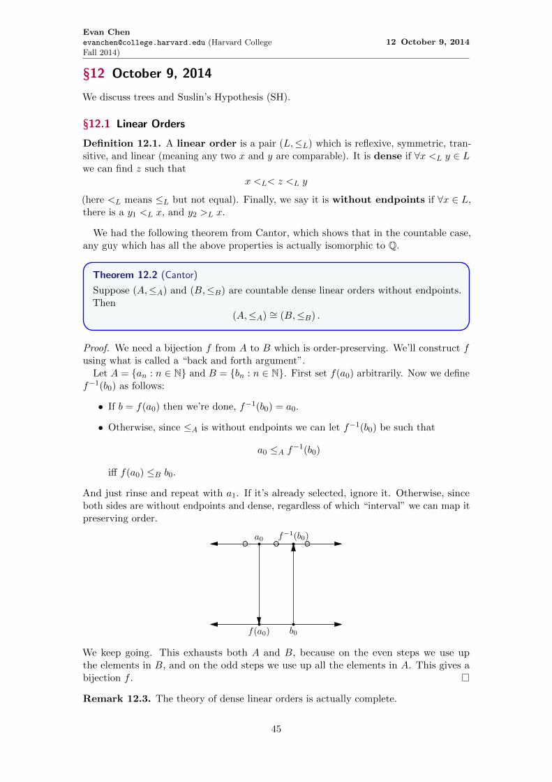
Evan [email protected] (Harvard CollegeFall 2014)
12 October 9, 2014
§12 October 9, 2014
We discuss trees and Suslin’s Hypothesis (SH).
§12.1 Linear Orders
Definition 12.1. A linear order is a pair (L,≤L) which is reflexive, symmetric, tran-sitive, and linear (meaning any two x and y are comparable). It is dense if ∀x <L y ∈ Lwe can find z such that
x <L< z <L y
(here <L means ≤L but not equal). Finally, we say it is without endpoints if ∀x ∈ L,there is a y1 <L x, and y2 >L x.
We had the following theorem from Cantor, which shows that in the countable case,any guy which has all the above properties is actually isomorphic to Q.
Theorem 12.2 (Cantor)
Suppose (A,≤A) and (B,≤B) are countable dense linear orders without endpoints.Then
(A,≤A) ∼= (B,≤B) .
Proof. We need a bijection f from A to B which is order-preserving. We’ll construct fusing what is called a “back and forth argument”.
Let A = an : n ∈ N and B = bn : n ∈ N. First set f(a0) arbitrarily. Now we definef−1(b0) as follows:
• If b = f(a0) then we’re done, f−1(b0) = a0.
• Otherwise, since ≤A is without endpoints we can let f−1(b0) be such that
a0 ≤A f−1(b0)
iff f(a0) ≤B b0.
And just rinse and repeat with a1. If it’s already selected, ignore it. Otherwise, sinceboth sides are without endpoints and dense, regardless of which “interval” we can map itpreserving order.
a0
f(a0) b0
f−1(b0)
We keep going. This exhausts both A and B, because on the even steps we use upthe elements in B, and on the odd steps we use up all the elements in A. This gives abijection f .
Remark 12.3. The theory of dense linear orders is actually complete.
45
Evan [email protected] (Harvard CollegeFall 2014)
12 October 9, 2014
§12.2 Intermission
Question 12.4. Can you generalize the proof to arbitrary cardinalities?
First, let us construct a dense linear order without endpoints of cardinality ℵ1. Considerthe set
A = Q× ω1
sorted lexicographically. This clearly works. This has a structure of ω1 embedded in it.So we have like a chain
A = Q0,Q1, . . . ,Qα, . . .
On the other hand we can just run this the other way.
B = . . . ,Qα, . . . ,Q1,Q0.
Consider ( 12014 , 0). In A, it has countably many things to its left. But every guy in B
has uncountably many things to its right. Hence no bijection exists.We can also do Q × (ω1 + 1), which is not isomorphic to A. You have a “maximal”
Q-blob Qω1 , and there’s intuitively no way to map this into A. (Check this!)
§12.3 Separable complete linear orders
Definition 12.5. A linear order (L,≤L) is complete if whenever A ⊆ L has an upperbound5, then there is a least upper bound, and similarly for sets bounded below.
Definition 12.6. We say (L,≤L) is separable if there exists a countable D ⊆ L forwhich (D,≤L) is dense.
Now we can prove a generalization of something Cantor did.
Theorem 12.7 (Cantor)
Suppose (A,≤A) and (B,≤B) are dense linear orders without endpoints, which areboth complete and separable. Then (A,≤A) ∼= (B,≤B).
Here we’ve replaced “countable” with “complete and separable”.
Proof. Take A ⊂ A which is countable and dense,6 and similarly define B. Evidently ourfirst theorem implies
(A,≤A) ∼= (B,≤B)
(just check all the conditions). Let f be the bijection from A to B. We want to lift thisto f : A→ B. This is easy enough: for any a /∈ A
f(a) = sup≤Bf(a) | a ≤A a .
We can take sup’s by completeness.To prove this is order-preserving, just notice that if a1 <A a2 then we get some a ∈ A
between them, so f(a) separates them. (In particular f is injective.)To prove f is surjective, look at any b ∈ B, take the downwards interval, and then use
the fact that A is complete.
In particular, (R,≤R) is the unique dense linear order without endpoints which iscomplete and separable (note that (Q,≤Q) witness separability).
5Meaning there exists a z ∈ L such that a ≤L z for all a ∈ A.6Think of these as “glowing special points” that are scattered all throughout A.
46
Evan [email protected] (Harvard CollegeFall 2014)
12 October 9, 2014
§12.4 Suslin property
Definition 12.8. A linear order (L,≤L) has the Suslin property if any collection ofdisjoint open intervals is countable. Here an open interval is one of the form
(a, b)def= z ∈ L | a <L z <L b .
It might seem that you should be able to pick ω1 into R, but in fact R does have theSuslin property – any open interval contains a rational number, so you can pick at mostcountably many. (But you can embed ε0 into R!)
Lemma 12.9
If a linear order (L,≤) is separable then it has the Suslin property.
Proof. Let D be a collection of disjoint open intervals, and let L be the dense countablesubset. By Separability, each open interval contains a distinct element of L.
So we can’t embed (ω1,∈) into there, but we can get order-preserving maps from(ω,∈), (ωω,∈), (ε0,∈), . . . . Now is it true that you can embed any α < ω1 in there?
Not sure. We can try transfinite induction. Embedding in (R,≤R) is the same as((−∞, 0),≤R), giving us space on the right to work with. For the transfinite inductionthe successor case is clear, but for limit ordinals λ we must somehow use the fact that λis countable (since the induction fails at λ = ω1).
Suppose λ is a limit less than ω1.7 So for each α we have an fα : α→ R and a bijectionπ : λ→ N.
Question 12.10 (Suslin’s Hypothesis). Is (R,≤R) the unique dense linear order withoutendpoints which is both complete and has the Suslin property?
Notice that SP is weaker than separable, and if we replace SP with separable then theanswer is “yes”.
Definition 12.11. We call a Suslin line any other ordering with this property; that is,a dense linear order which is complete, has the Suslin property, but is not separable.
SH is the conjecture that no Suslin lines exist. This would be weird. We can only liedown countably many disjoint union intervals, but the reason is not because we can picka “rational” in every set (by “rational” we mean an element of a separable set).
Theorem 12.12
If ZFC is consistent, then
(a) ZFC + SH is consistent
(b) ZFC + ¬ SH is consistent.
This is proved using something called a Suslin tree. We have the following theorems,which we won’t prove.
7This can terribly be written as λ ∈ Lim ∩ ω1.
47
Evan [email protected] (Harvard CollegeFall 2014)
12 October 9, 2014
Theorem 12.13
There is a Suslin line if and only if there is a Suslin tree.
Theorem 12.14
Let L be the constructible universe (“up next”). Then if V = L, we have a Suslinetree ¬ SH.
But we can use a trick called “forcing” as follows: we can put a branch through it to killit, but then more trees come up, and then it’s just massive deforestation. That’s how weget another direction.
48
Evan [email protected] (Harvard CollegeFall 2014)
13 October 14, 2014
§13 October 14, 2014
Sick day. What happened?
§13.1 Sparse Review
Given a model (M,E), an assignment to
VAR = (7, i) | i ∈ ω
is a function s : VAR → M . We think of s(“x′′0) = s((7, 0)) = a ∈ M . Basically, weassign every variable to something in M .
Given a formula ϕ, ϕ(x0, . . . , xn) where the free variables are x0, . . . , xn and anassignment s : VAR→M , the only part that matters for is s(“x′′0), . . .
We’re going to be lazy and write things like x ∈ y, even though x and y are not actuallyofficial variables.
Often we write(M,E) φ[~a]
where ~a is really just the part of s : VAR→M that is relevant, namely
~a = (s(x0), . . . , s(xn)) .
(Remember means “satisfies”.)Definitions of ∆0, Σn, Πn.∆0 corresponds to having no unbounded ∀ and ∃. It means you don’t have to look
around things.
49
Evan [email protected] (Harvard CollegeFall 2014)
14 October 16, 2014
§14 October 16, 2014
Guest lecture! Today we discuss infinite combinatorics. Unfortunately in my illness Iarrived late and failed to get the guest’s name.
In finite combinatorics we studied partitions of numbers and rooted trees. Today wewill be discussion the generalizations of these to the transfinite.
§14.1 Partitions
We can think of a partition of S as writing
S = S0 t S1 t · · · t Sm−1
as just a function f : S → 0, . . . ,m − 1 (that is, f : S → m) specifying here to sendeach element of S.
Definition 14.1. For a set A, let [A]n be the subsets of size n; i.e.
[A]n = x ⊆ A | |A| = n .
Definition 14.2. Let δ be an infinite cardinal. We define a function f : S → δ to be aδ-partition of S. Given a δ-partition of the [A]n, a set H ⊆ A is called homogeneousfor f if f is constant on [H]n.
Remark 14.3. It’s helpful to think of f as a coloring function on the n-subsets. Homo-geneous corresponds to monochromatic.
§14.2 Infinite Ramsey Theorem
Example 14.4
It’s well-known from Ramsey theory that any six people, either three are mutualfriends or three are mutual stranger. We can rephrase this as saying: any 2-partitionof [6]2 has a homogeneous subset of size 3. (Here [6]2 are the edges, and we put theminto two colors.)
This is a consequence of the finite Ramsey theorem, but we’ll prove an infinite version.
Theorem 14.5 (Infinite Ramsey Theorem)
If A is an infinite set, and f : [A]n → m is an m-partition of the n-subsets of A, thenthere is some countably infinite H ≤ A homogeneous.
Here (and for the rest of the lecture), m and n will denote natural numbers.
Remark 14.6. When n = 2, this states that any m-coloring of an infinite graph has amonochromatic coloring.
Proof. We are going to repeatedly use Infinite Pigeonhole. If n = 1, then we are tryingto partition [A]1 = A into a finite pieces, so some part must be infinite, QED.
Now suppose it holds for n. Consider f : [A]n+1 → m. For a ∈ A, we define fa from[A− a]n → m by
fa(x) = f(x ∪ a).
50
Evan [email protected] (Harvard CollegeFall 2014)
14 October 16, 2014
By inductive hypothesis, each fa has an infinite homogeneous subset. Let H0 = A anda0 be arbitrary. For i < ω we define
Hi+1 ⊆ Hi infinite and homogeneous for fai
and then pick ai+1 ∈ Hi+1 − aj | j ≤ i.Now consider ai : i < ω. The point is that ai : i > k is homogeneous for fak . Let
the constant value of fak on ai : i ≥ k be g(i). By infinite pigeonhole there is an infinitesubset I on which g is constant, as necessary. Then ai : i ∈ I is the desired set.
The special case of the proof with m = 3 colors (RGB, anyone?) and n = 2 is moresuitable for an olympiad, but makes the above proof much more illuminating. Consideran infinite graph. Take a vertex v0. Some color emanates infinitely often from v0. Throwaway everything else. Take a new v1. Ignoring v0, some color emanates infinitely from v1.Throw away the other guys (but keep v1)! In this way we get a sequence v0, v1, . . . ofvertices, each with a color it really likes. By Pigeonhole, we can take an infinite subsetthat all like the same color. Done.
§14.3 Some negative results on partitions
Definition 14.7. If κ and δ are cardinals, and n ∈ N, and α is an ordinal we writeκ → (α)nδ if for every δ-partition of [k]n, there is a homogeneous set H ⊆ κ for thepartition, and H has size α.
Example 14.8
6→ (3)22 and ω → (ω)nm.
Note that you can increase κ and decrease α, so the → is “like” an inequality ≥.Why do we assume n ∈ N? It turns out if AC is given, then we have the follow-
ing.
Lemma 14.9
Assume AC. Then κ 6→ (ω)ω2 for any infinite cardinal κ.
Remark 14.10. People often drop the subscript 2.
Proof. Take a well-ordering ≺ of [κ]ω. We’ll split κ into two parts using f : [κ]ω → 2 by
f(A) =
1 A is ≺-minimal among the infinite subsets of A
0 otherwise.
Assume for contradiction there’s some homogeneous H ⊂ κ of size ω; WLOG it’scountable.
If H isn’t ≺-minimal, then consider an infinite A ∈ H which is. Then f colors A by 1.But H is also an ω-subset of H, so f colors H by 0, contradiction.
So H must be ≺-minimal, and since H is homegeneous, so must every infinite subsetof H. Select an infinite subset A0 ∈ H such that H −A0 is also infinite. By looking atthe elements missed by A0, we can create a chain
A0 ⊆ A1 ⊆ A2 ⊆ . . .
51
Evan [email protected] (Harvard CollegeFall 2014)
14 October 16, 2014
But now we can obtain a decreasing ≺ chain
H ⊇ A0 A1 A2 . . . .
Indeed, each Ai is infinite but is ≺-minimal with respect to all its infinite subsets,including Ai−1. Boom!
Lemma 14.11
Assume AC. For any κ, 2κ 6→ (κ+)22.
Proof. Let⟨xα | α < 2k
⟩enumerate the binary sequences of κ; i.e. the functions from κ
to 2. For each “edge” α, β consider the coloring where
α < β → (f(α, β) ⇐⇒ xα <lex xβ.
Assume for contradiction there’s a homogeneous (think monochromatic) subsequence〈xα : α ∈ H〉, and WLOG it is increasing.
For each i we define
βi = minβ | β ≥ 1 + sup
j<iβj and
∃α > 1 + supj<i
αj , α ∈ H
and β has 1 in the α digit.
αi = minα ∈ H | α > 1 + sup
j<iαj
and βi has 1 in the α digit.
Set the sup’s as 0 when i = 0.Basically what this does is that as i grows, more digits get fixed. Supremum exists by
regularity of κ+. So you get screwed by the time you get to xκ.
Remark 14.12. This is highly similar to the proof that you can’t have an ℵ1 increasingsequence of real numbers.
Corollary 14.13
2κ 6→ (2κ)22.
Proof. 2κ ≥ κ+.
§14.4 Large Cardinals
Definition 14.14. A cardinal κ is called weakly compact if κ→ (κ)22.
Corollary 14.15
If κ is weakly compact, κ is inaccessible.
52
Evan [email protected] (Harvard CollegeFall 2014)
14 October 16, 2014
Proof. By above stuff, we clearly have κ > 2λ for all λ < κ.Assume for contradiction that κ is singular. Then κ =
⋃i<λAi where λ < κ and
|Ai| < κ. Define f : [k]2 → 2 by
f(α, β) = 1 ⇐⇒ ∃i < λ : α, β ∈ Ai.
§14.5 Trees
Definition 14.16. A tree is a poset (T,<) such that for every x ∈ T , the set
predT (x) = y ∈ T | y < x
is well-ordered by <. The height of any x is ht(x) = ot(predT (x)) and Tα is the set ofx’s with height α, meaning
Tα = x ∈ T | ht(x) = α .
The height of the whole tree is the smallest α with Tα 6= 0, i.e.
ht(T ) = min α : Tα = ∅ .
A branch through T is a maximal linear subset. A κ-tree is a tree of height κ whoselevels each have less than κ.
Example 14.17
The tree 2<ω is an ω-tree. The tree ω<ω has size ω, but it is very fat and not anω-tree.
Definition 14.18. An Aronszajn tree (pronounced EH-rin-shine) is a κ-tree withouta branch of size κ.
Lemma 14.19 (Konig’s Lemma)
There is no ℵ0-Aronszajn tree.
Proof. At each level there’s finitely many guys. So some branch is infinite. Now go upthe tree greedily.
Lemma 14.20 (Aronszajn)
There is an ℵ1-Aronszajn tree.
53
Evan [email protected] (Harvard CollegeFall 2014)
15 October 21, 2014
§15 October 21, 2014
Constructability, Model Theory, . . .
§15.1 Definability
Definition 15.1. Given (M,E) a model in LST, we say that a relation X ⊆ Mn is(M,E)-definable by ϕ(x1, . . . , xn) if
X = ~a ∈Mn | (M,E) φ[~a] .
We say X is (M,E)-definable if such a ϕ exists.
Definition 15.2. We say X is definable in (M,E) with parameters if there is aformula φ(x1, . . . , xn, y1, . . . , ym) and a parameter sequence ~b ∈Mm such that
X =~a ∈Mn | (M,E) ϕ[~a~b]
.
Remark 15.3. Everything in M is definable in (M,E) with parameters. Take b ∈Mand consider the formula “x = b”. This has one free variable and one parameter.
Remark 15.4. We’ll say a ∈M is definable if a is definable.
Example 15.5
We can write down the formula defining “is an ordinal”. We can expand the machinecode for transitive: ∀y ∈ x(y ⊆ x), or ∀y ∈ x(∀z ∈ y(z ∈ x)). This is ∆0 because ithas no unbounded parameters. Similarly expand “well-ordered by ∈”.
Example 15.6
∅ is ∆0 definable. Write the formula ∀y ∈ x(y 6= y).
We are mainly interested in ∈-models, where M is transitive and ∈ |M×M = E. Wewill often write this as (M,∈).
§15.2 Fragments of the Universe
Let’s see what is definable over the structure (Vω,∈).
Example 15.7
ω = 0, 1, . . . is ∆0 definable without parameters in (Vω,∈). Get
a ∈ Vω | (Vω,∈) ϕ[a] = 0, 1, . . . .
where ϕ means “is an ordinal”.
Example 15.8
a ∈ Vω1 | (Vω1 ,∈) ϕ[a] = ω1 and a ∈ V | (V,∈) ϕ[a] = On.
54
Evan [email protected] (Harvard CollegeFall 2014)
15 October 21, 2014
Lemma 15.9
Suppose (M,∈) and (N,∈) are two transitive ∈-models. Moreover, suppose M ⊆ N .Let ϕ(x1, . . . , xn) be a formula in LST. Let ~a ∈Mn be a parameter sequence. Then
(a) If ϕ ∈ ∆0, then (M,∈) φ[~a] ⇐⇒ (N,∈) φ[~a].
(b) If ϕ ∈ Σ1, then (M,∈) φ[~a] implies (N,∈) φ[~a], but the converse fails.
(c) If ϕ ∈ Π1, then (N,∈) φ[~a] implies (M,∈) φ[~a], but the converse fails.
These are called ∆0-absoluteness, upward Σ1-absoluteness, and downward Π1-absoluteness.This is actually intuitively clear. In the first case, since ϕ ∈ ∆0, then truth depends onlyon things internal to ~a, and M and N have the same information in this case. In thesecond case, we have some existence qualifiers, but setting these to things in M is fine inN as well. Similarly for the third case.
Proof. We prove (a) by induction on formula complexity. In the base case, we haveseveral cases. The first is φ is “x1 ∈ x2”. Given (a1, a2) = ~a ∈M2, we have
(M,∈) a1 ∈ a2 ⇐⇒ (N,∈) a1 ∈ a2.
Well, duh. We also have “x1 = x2”, which is clear.For the inductive step, we assume the statement holds for φ(x1, . . . , xn) and ψ(y1, . . . , yn).
We just check ¬φ(x1, . . . , xn) and φ(x1, . . . , xn) ∧ ψ(y1, . . . , ym).Do stuff with the other quantifiers. We need the transitivity condition at the bounded
quantifier step. If M thinks there exists x in the parameter a, we need N to also thinkthat. Writing it out
(M,∈) ∃y ∈ x1φ(y, x1, , , .xn)[~a]
means by definition∃b ∈ a1 : b ∈M and (M,∈) φ[b, a1]. (1)
On the other end we have
(N,∈) ∃y ∈ x1φ(y, x1, , , .xn)[~a]
means by definition∃b ∈ a1 : b ∈ N and (N,∈) φ[b, a1]. (2)
So we need to show the witness statements (1) and (2) are equivalent. To show (1) implies(2), we only need M ⊆ N . For the other direction, though, we do need transitivity; weknow b ∈ a1, b ∈ N , a1 ∈ M , but we want b ∈ M and that doesn’t follow unless M istransitive!
For (b), (c) do similar things. Invoke (a) for convenience.
§15.3 Definable sets
Definition 15.10. For (M,∈), with M transitive, and define
DefM = X ⊆M | X definable on (M,∈) with parameters .
Remark 15.11. We clearly have M ⊆ DefM ⊆ P(M).
Fact 15.12. If |M | = n ∈ N, then∣∣DefM
∣∣ = 2n.
55
Evan [email protected] (Harvard CollegeFall 2014)
15 October 21, 2014
Fact 15.13. If |M | = α ≥ ω, then
∣∣DefM∣∣ = α× ℵ0 = α.
Exercise 15.14. Suppose (M,∈) is an ∈-model with M transitive.
(1) (M,∈) Extensionality, Foundation.
(2) (M,∈) ∅Emptyset if and only if ∅ ∈M , i.e. M 6= ∅. (Just note that “x = ∅′′ is∆0.)
(3) M Pairing if and only if ∀x, y ∈M we have x, y ∈M .
(4) . . .
(5) . . .
(6) (M,∈) Infinity when ω ∈M .
(7) (M,∈) Comprehension if and only if for every C ∈ DefM and for all a ∈M , wehave C ∩ a ∈M .
The key is ∆0 – this lets us move back and forth between (M,∈) and V .
56
Evan [email protected] (Harvard CollegeFall 2014)
16 October 23, 2014
§16 October 23, 2014
Today we cover reflection. In what follows, the LST models are not necessarily transitive.
§16.1 Model theory notions
Definition 16.1. Suppose M = (M,E) and M ′ = (M ′, E′) are LST-models. We sayM is a substructure of M ′, written M ⊆M ′, if M ⊆M ′ and E = E′ ∩ (M ×M).
Definition 16.2. We say M is an elementary substructure of M ′, written M ≺M ′,if for all φ in LST and ~a ∈Mn, M φ[~a] ⇐⇒ M ′ φ[~a].
Theorem 16.3 (Tarski-Vaught Test)
Suppose M , M ′ are LST-models such that M ⊆M ′. Then M ≺M ′ if and only ifthe following condition holds: Let φ be a sentence in LST and ~b ∈Mn. If ∃a ∈M ′such that M ′ φ[a,~b] then there exists a ∈M such that M ′ φ[a,~b].
Proof. First, we show (1) implies (2). Assume M ≺ M ′. Fix φ in LST and ~b ∈ Mn.Suppose ∃a ∈M ′ such that M ′ φ[a,~b]. Then M ′ ∃aφ[a,~b]. Since M ≺M ′,
M ∃aφ[a,~b].
Fix such an a ∈M . So M φ[~a,~b]. But M ≺M ′, so
M ′ φ[a,~b]
as needed.The converse is the interesting direction. We’ll prove (1) by induction on formula
complexity. The base case is Σ0 formulas. a = b means
M a = b ⇐⇒ a = b ⇐⇒ M ′ a = b.
Now a ∈ b is
M a ∈ b ⇐⇒ (a, b) ∈ E ⇐⇒ (a, b) ∈ E′ ⇐⇒ M ′ a ∈ b.
Then for some last things. Negation ¬ and or ∨ is immediate. We also need boundedquantifiers. Assume it’s true for φ, so
M φ[~b] ⇐⇒ M ′ φ[~b]
Show that for a ∈M ,
M ∃x ∈ aφ(x, b) ⇐⇒ ∃a ∈M,a ∈ a,M φ[a,~b].
Hence ∃a ∈M , a ∈ a, such that M ′φ[a,~b].Then for the inductive step. Suppose that M and M ′ satisfy the same formulas for
Πn formulas (the Σn case follows by negation). Want to show Σn+1 Fix φ ∈ Σn+1, say
φ = ∃xψ(x, y1, . . . , yn)
where ψ ∈ Πn. SupposeM ∃xψ[x,~b].
57
Evan [email protected] (Harvard CollegeFall 2014)
16 October 23, 2014
Pick a ∈M such thatM ψ[a,~b]
so since M ≺Πn M ′ we haveM ′ ψ[a,~b].
HenceM ′ ∃xψ[x,~b].
Hence we have prove than
M ∃xψ[x,~b] =⇒ M ′ ∃xψ[x,~b].
We need the converse now. So far we haven’t used the Tarski-Vaught condition; we invokeit now and then repeat the proof in the opposite direction. Indeed, just take a ∈M ′ suchthat M ′ [a,~b]. Then ∃a ∈ M such that M ′ ψ[a,~b]. The inductive hypothesis thenfinishes the proof.
Intuitively, what this is saying that M ≺ M ′ if for some formula φ, if we have awitness a in M ′ then we can also get a witness in M .
§16.2 Reflection
Now for the cool stuff.
Definition 16.4. Suppose κ is a regular uncountable cardinal. Then C ⊆ κ is a club(short for “closed unbounded”) if the following holds for all α < κ
• There exists β ∈ C with β > α.
• If α = sup(C ∩ α), then α ∈ C.
Theorem 16.5 (Reflection)
Let κ be a regular uncountable cardinal. Let 〈Mα : α < κ〉 be such that
(1) Each Mα = (Mα, Eα) is an LST-model.
(2) Mα ⊆Mβ for all α < β < κ.
(3) |Mα| < κ for any α.
(4) Mλ =⋃α<λMα for any limit λ.
We define M = (M,E), where M =⋃α<κMα and E =
⋃α<κEα. Then the set
C = α < κ |Mα ≺M
is a club in κ.
Remark 16.6. It follows from this that if α < β and α, β ∈ C, then Mα ≺Mβ.
Proof. Let λ be a limit cardinal less than κ. We wish to show that C ∩ λ is unboundedin κ. We wish to show λ ∈ C, i.e. that Mλ ≺M . In other words, for any φ in LST and~b ∈Mn
λ we want the equivalence
Mλ φ[~b] ⇐⇒ M φ[~b].
58
Evan [email protected] (Harvard CollegeFall 2014)
16 October 23, 2014
Well, ~b gets covered by by some Mα since λ is a limit dude. Now we want to check theTarski-Vaught test. Suppose a ∈ M , M φ[a,~b]. We want to show there is a ∈ Mλ,M φ[a,~b]. So we go down to Mα:
M ∃xϕ[x,~b] =⇒ Mα ∃xϕ[x,~b]
and blah blah blah.So this shows that C is closed. That’s not too interesting, because for all we know C
might just be empty. But now we’re going to show C is unbounded, which is far moreinteresting. For φ in LST, let
fφ : κ→ κ
by sending α to the least β < κ such that for all ~b ∈Mα, if there exists a ∈M such thatM φ[a,~b] then ∃a ∈Mβ such that M φ[a,~b].
We claim this is well-defined. There are only |Mα|n many possible choices of ~b, and inparticular there are fewer than κ of these (this is why we assume |Mα| < κ). Otherwise,we can construct a cofinal map from |Mn
α | into κ by mapping each vector ~b into a β forwhich the proposition fails. And that’s impossible since κ is regular!
In other words, what we’ve done is fix φ and then use Tarski-Vaught on all the ~b ∈Mnα .
Now let g : κ→ κ be defined by
α 7→ supφ∈LST
fφ(α).
Since κ is regular and there are only countably many formulas, g(α) is well-defined.Check that if α has the property that g maps α into itself (in other words, α is closed
under g), then by the Tarski-Vaught test, we have Mα ≺M .So it suffices to show there are arbitrarily large α < κ which are closed under g. Fix
α0. Let α1 = g(α0), et cetera and define
α = supn<ω
αn.
This α is closed under g, and by making α0 arbitrarily large we can make α as large aswe like.
§16.3 Variations
Theorem 16.7
Suppose φ is in LST and ~b ∈ V n. If V φ[~b], then there exists α such that Vα ` φ[~b].
Why is this called reflection? Basically it means any statement φ one tries to make aboutV is destined to fail in the sense that some level Vα will also have the statement.
Theorem 16.8
C = α ∈ On | Vα ≺Σn V is a club in On.
59
Evan [email protected] (Harvard CollegeFall 2014)
17 October 28, 2014
§17 October 28, 2014
Laptop sick day. TODO: fill in.
60
Evan [email protected] (Harvard CollegeFall 2014)
18 October 30, 2014
§18 October 30, 2014
Continuation of last time. (Guess whose laptop was dead?)
§18.1 Completing the proof of a theorem
We were proving Lκ ZF
Proof. See notes. TODO: fill in later. Reflection Theorem is useful because the setup isLκ =
⋃α<κ Lα.
. . .Let F ∈ DefLκ and F : Lκ → Lκ. We want to show for any set a, F applied pointwise
to a lives inside κ.Assume not. Let α < κ be such that a ∈ Lα. We can shoot each element of Lα onto|α| < κ, and then we get a cofinal map from |α| into κ, contradiction.
§18.2 The statement Lκ V = L
We will show Lκ gives V = L, AC, and CH.We need to prove that
∀x∃α (x ∈ Lα) .
This might seem since by definition Lκ =⋃α<κ Lα. But this particular statement is in
V . We need to prove it in Lκ; i.e. while it’s obvious that V V = L, we don’t haveLκ V = L.
Let x = Lα. We want to decide whether Lκ (x = Lα). In other words, we definedLα in V , and we want to check we get the same thing as if we run the definition in L (orLκ).
Like assuming ZFC is consistent, we can construct a model M∗ of ZFC which is notwell-founded by adding on the condition α1 > α2, α2 > α3, . . . . This is consistent bycompactness (look it up): for the model to be inconsistent, it must have a finite set ofinconsistent statements. And if we run the definition of L in here, we get something else
In still other words, what we really want to do is show that if we run the definition ofLκ inside itself, we get all of Lκ. So our goal it look at the definition of 〈Lα : α < κ〉 andcheck that it is simple enough that we have absoluteness. Since Lκ is transitive, we’dbe done if this was ∆0 – but it’s not. In fact, we will show it is Σ1. This is sufficientbecause we then have
Lκ (x ∈ Lα) =⇒ V (x ∈ Lα) .
For this we use something like Godel encoding. First we need to get the language, whichwe’ve already done. Then we have to define what a term is. Then we need to define aformula sequence; it’s just going to be a finite sequence where you build up the formula.Next you define the length of a formula. It turns out that all these things so far are ∆0.Finally you define satisfaction sequence and definability in Σ1.
In the end by encoding syntax (with some fairly scary computations) that
• “x is the αth level of the L-hierarchy”, that is, Lα, is Σ1-definable.
• “x is constructible” is Σ1 since it is ∃y, α (Lev(y, α) ∧ x ∈ y).
• V = L is the statement ∀x (y is constructible), so it is Π2.
Exercise 18.1. Assume λ > ω is a limit ordinal. Show that for all α such that ω < α < λ,we have
Lλ DEF(Lα+1, Lα).
61
Evan [email protected] (Harvard CollegeFall 2014)
18 October 30, 2014
Here the Lα+1 and Lα are the real thing.
Proof. Check that DEF(x, y) is Σ1. Check that Lα+1 is a Σ1 formula.
The converse of what we want is also a thing.
Theorem 18.2
If M is transitive and M V = L then M = Lλ for some limit ordinal λ.
Proof. Since M V = L, and α first appears in Lα+1, the sup of the ordinals in M mustbe a limit ordinal, say λ.
Consider x ∈M . Since M V = L, there exists b, α such that M LEV(b, α)∧ x ∈ b.But (and this is the point), the statement LEV(b, α) is Σ1. So by Σ1-upward absoluteness,we get V LEV(b, α). Hence b = Lα.
Thus x ∈ b = Lα. Hence we showed that for all x ∈ M , x ∈ Lα for some α < λ.Consequently M ⊆ Lλ. Thus M = Lλ.
Now here’s what we want.
Theorem 18.3
If λ is a limit ordinal, then Lλ V = L.
Proof. Fix x ∈ Lλ. Let α < λ be such that x ∈ Lα. It suffices to show that Lλ LEV(Lα, α).
We expand the definition of LEV. Use the fact that Lλ has the function sequencewitnessing this Σ1 fact.
Like basically, it turns out there’s a ϕ, f such that
V ∃f (ϕ[f, Lα, α)
and you can show f ∈ Lλ.
The key point is the following lemma.
Lemma 18.4
If λ is a limit ordinal then for all α < λ,
〈Lβ | β < α〉 ∈ Lλ.
In fact,〈Lβ | β < λ〉 = DefLλ .
Corollary 18.5
In ZFC+, Lκ V = L. So we have Lκ ZF + (V = L).
Remark 18.6. We only need the κ condition to guarantee that V = L holds, but weneed regularity to cause it satisfy ZF. As an example, both models Lω, Lω+ω impliesV = L but not ZF.
62
Evan [email protected] (Harvard CollegeFall 2014)
18 October 30, 2014
§18.3 A Nice application of Reflection
Proposition 18.7
Assuming ZFC+, there exists a countable α for which Lα satisfies ZF.
Proof. By Reflection, the set D = α < κ | Lα ≺ Lκ is a club in κ. Hence for eachα ∈ D, we have Lα ZF.
Using Choice (Lκ AC), we can get a model M ≺ Lκ such that M ∈ Lκ and |M | = ℵ0.(This is the same argument as last time right before we did the Mostowski collapse.)Now exactly like last time we can let M be the transitive collapse of M ; hence M istransitive and M satisfies ZF and V = L. The only transitive sets with V = L are Lα bythe earlier theorem, and since M is countable, we have α < ω1.
§18.4 A sketch of the proof that Lκ AC
Induction. Assume we have a well-ordering of Lα. We wish to get an ordering of Lα+1.But
Lα+1 = DefLα =x ∈ Lα | Lα ϕ[x,~b]
.
Here φ is in LST and ~b is a vector of Lα We can well order the countably many formulasof ϕi, we can order ~b lexicographically, and then lexicographically order the entire set.
The limit ordinals are just unions.In fact we get more that Choice in Lκ – we can order the entire universe. More on
that next time.
63
Evan [email protected] (Harvard CollegeFall 2014)
19 November 4, 2014
§19 November 4, 2014
Today we will finish constructibility. The goal is to show that Lκ implies AC, GCH, anda principle to be defined later.
§19.1 Axiom of Choice
Theorem 19.1
Hence we have shown that ZF + (V = L) =⇒ AC. Hence Lκ AC.
You need κ to be inaccessible to get κ ZF. But you only need κ a limit to get V = L.
Proof. We want a function F from the ω, ω + 1, . . . to V sending α to a <α such thatfor α ≥ ω, the following conditions hold:
(1) <α is a well-ordering of Lα.
(2) α < β =⇒ <α⊆<β. Moreover, for any x ∈ Lα and y ∈ Lβ − Lα, we have x <β y.
(3) There exists a Σ1 formula φ(x0, x1, x2) such that for every limit ordinal λ ≥ ω, wehave
(Lλ φ[a, x, Vω]) ⇐⇒ (α ∈ On ∨ x =<α).
Here’s a sketch of how to do this. We can define <ω because Vω consists of a bunch offinite layers. Let 〈ϕi : i < ω〉 be a Σ1-definable well-ordering of all the formulas in LST(possible since they live in Vω). So you can just lex order everything!
To be explicit – suppose we have <α defined and want to define <α+1. We have bydefinition
Lα+1 =x ⊆ Lα | x ∈ DefLα
So every element of Lα+1 is of the form
x = z ∈ Lα | ϕi[z, a1, . . . , an]
so we can associate with each x a tuple (i, a1, . . . , an) and then just lex-order it. (Sinceyou can possibly get multiple tuples, you should take the smallest one.)
For λ a limit ordinal, we write <λ=⋃α<λ <α.
§19.2 GCH
Lemma 19.2 (Condensation)
Assume ZF + (V = L). Suppose X ≺ Lλ is an elementary substructure which istransitive. Then
(X,∈) ∼= Lλ
for some limit ordinal λ.
Remark 19.3. It follows that if X is an elementary substructure of Lω (not necessarilytransitive) then X ∼= Lω.
64
Evan [email protected] (Harvard CollegeFall 2014)
19 November 4, 2014
Proof. Since ∈ is well-founded and extensional, we can take the Mostowski collapse of(X,∈) to get π : (X,∈) → (X,∈), where X is transitive. We know Lλ (V = L), soX (V = L) (by the assumption X ≺ Lλ), thus X (V = L). But we already provedthat the transitive sets which satisfy V = L are precisely Lλ.
It remains to show that λ is a limit. But this follows from the fact that Lλ thinks “∀α,α+ 1 exists”, and this propagates down to Lλ, QED.
Theorem 19.4
ZF + (V = L) =⇒ GCH, and hence Lκ GCH. Here GCH is the statementκ+ = 2κ for any infinite cardinal κ.
Proof. Note that ZF + (V = L) implies AC, so we use Choice freely here.By Cantor, 2κ ≥ κ+, so it suffices to prove that 2κ ≤ κ+. But we also showed in
homework that|Lκ+ | = κ+.
(Actually, we proved |Lα| = |α| for any α.) Hence, it suffices to show that any subsetA ⊆ κ in L is actually in Lκ+ , because then we’ve squeezed 2κ into a space of cardinalityκ+. In other words, we will show P(A) ⊆ Lκ+ where the power set is taken over L.
Consider any A ⊆ κ. Let λ > κ be a limit. As in the proof of Reflection, we cantake X ≺ Lλ such that |X| = κ, A ∈ X, and κ ⊆ X. Let π : (X,∈) → (Lλ,∈) be thetransitive collapse in Condensation. We claim that A ∈ Lλ. Indeed,
π(A) = π(γ) | γ ∈ A .
But π acts as the identity on κ (check this by transfinite induction), and it follows thatπ(A) = A.
However, ∣∣Lλ∣∣ = |X| = κ < κ+.
Thus A = π(A) ∈ Lλ.
§19.3 Hulls
Let me write down the details for “as in the proof of reflection”, since I’ve messed thisup twice. Here’s what we do. By Tarski-Vaight it suffices to find an X such that for allϕ in LST and for all ~b ∈ X, if we have witnesses a ∈ Lλ establishing Lλ ϕ[a,~b], thenwe can find a witness a ∈ X establishing
Lλ ϕ[a,~b].
Now we define X by recursion as follows. Set
X0 = κ ∪ A.
This is our “initial set” of things we want X to have at the end of the day. Then we let
X1 =⋃
φ∈LST,~b∈Xω0
Lλ∃zφ[z,~b]
a ∈ Lλ | a is <λ-minimal andLλ [a,~b]
.
OK, that’s retarded because the union is over a bunch of singleton sets. But I thinkthat makes the point. Basically, we’ve thrown in parameters in Lλ such that X1 satisfies
65
Evan [email protected] (Harvard CollegeFall 2014)
19 November 4, 2014
Tarski-Vaught for all φ when the parameters are in X0. The problem is now we havesome elements in X1 \X0 which can also be parameters. So we construct Xn+1 based onXn in the same way.
Hence Xn+1 works for parameters in Xn, and moreover Xn ⊆ Xn+1. By takingX =
⋃n<ωXn, now X satisfies the Tarski-Vaught test.
Now we claim |X| = |X0| = κ ≥ ω. This just follows that any step, we only added inω · κω = κ many things.
Apparently these things are called hulls.
Theorem 19.5
Assume ZFC+, so κ is a strongly inaccesible cardinal. There is a countable transitivemodel of ZFC.
Proof. As in the proof of reflection, one can exhibit X ≺ Vκ countable. Then take theMostowski collapse of X.
Details: let X0 = ∅. We construct a sequence of countable sets Xn inductively asfollows. Consider a sentence φ ∈ LST and for a parameter sequence b ∈ Xn such thatVκ ∃zφ[z, b]. Then we take the any such z, and add it into Xn. We let Xn+1 be theresult.
Since Xn was countable, the set φ×X<ωn of possible pairs of sentences and parameters
is countable, and hence we add in at most countably many new elements; hence Xn+1 iscountable.
Then X =⋃Xn is countable and is an elementary substructure of Vκ. Now take the
Mostowski collapse of X.
§19.4 Summary
We have shown the following.
• ZF + (V = L) implies AC and GCH.
• Lκ ZF + (V = L).
• Lκ ZF + (CH).
So assuming ZFC+, we have demonstrated that ZFC cannot establish ¬CH. Later wewill use forcing to show that ZFC cannot prove CH either.
But actually we showed more than L CH. We showed that every real number (subsetsof N) appears in Lω1 . So we ask, where do the real numbers appear? For which α do wehave get a new real at some level? That’s searching for solutions to
P(ω) ∩ Lα+1 ) P (ω) ∩ Lα.
Fact 19.6. Suppose P(ω) ∩ Lλ+1 6= P (ω) ∩ Lλ. Then there exists a function f ∈ Lλ+1
such that f : ω → Lλ which is onto.
In other words, the witness that Lλ is countable appears immediately after a new realnumber appears.
Next time: β-gap theorem.
66
Evan [email protected] (Harvard CollegeFall 2014)
20 November 6, 2014
§20 November 6, 2014
We’ll finish with some more consequences of condensation.
§20.1 β-Gaps
Definition 20.1. For ordinals α, β a β-gap is a segment
[α, α+ β] = γ ordinal | α ≤ γ ≤ α+ β
such that P (ω) ∩ Lγ is empty for each γ in the interval. In other words, P (ω) ∩(Lα+β − Lα).
Theorem 20.2
Assume ZF and V = L. Then for all β < ω1 there is a β-gap [α, α + β] such thatα+ β < ω1.
Proof. We’re interested in gaps less than ω1 since all the reals appear by Lω1 . Like clearlywe can select a gap
[α′, α′ + β] ∈ Lω2 .
Actually, we are going to use the obvious statement to prove the non-obvious statement.Using hulls, we can let X ≺ Lω2 be countable such that [α′, α′ + β] ⊆ X. Hence,
Lω2 (P (ω) ∩ (Lα′+β − Lα′) = ∅
).
Hence X satisfies this.Denoting by π : X → Lλ be the Mostowski collapse; we have λ < ω1. We set
α = π(α′) an ordinal (since “is an ordinal” is ∆0). By the definition of π, we see thatα + 1 = π(α′ + 1), and so on. Hence the segment is preserved. Now since Lλ is anelementary substructure of Lω1 it follows that [α, α+ β] is still a gap. To be pedantic,
Lλ (P(π(ω)) ∩
(Lπ(α′)+π(β) \ Lπ(α′)
)= ∅
).
§20.2 A Taste of Fine Structure
Work in ZF + (V = L) and let λ be a limit ordinal. In our proof of GCH, we showedthat for any cardinal κ, if A ⊆ κ appears in Lλ+1 \ Lλ, then in L there is a functionf : κ→ Lλ which is onto. This implies that |Lλ| = κ; from this CH follows.
Now we actually claim that the collapsing function exists in Lλ+1. In other words,the moment a new subset appears above Lλ, we immediately also see a witness f thatcollapses all of Lλ onto κ.
Theorem 20.3
Assume ZF and V = L. Let κ be a cardinal and A any subset of κ such thatA = Lλ+1 \ Lλ for some limit ordinal λ. Then there exists a function f definableover Lλ which collapses κ onto Lλ.
67
Evan [email protected] (Harvard CollegeFall 2014)
20 November 6, 2014
Proof. We have an order <L of Lλ which is Σ1-definable. Let ψ be the formula givingLλ. By assumption,
A = x ∈ Lλ | Lλ ϕA[x, pA]for some formula φA and parameters pA in Lλ. It is important right now that we selectpA to be the <L-least parameter which works for the choice of ϕA.
Using hulls, we let X be an elementary substructure of Lλ such that κ ∪ pA ⊆ X.(Note that X may be a class here.) Via condensation again we take the Mostowskicollapse
π : X → Lλ.
Claim. λ = λ! That means the collapse did not actually collapse anything.
Proof. We wish to show A is in Lλ+1 − Lλ; hence it suffices to show A is definable overLλ. Since κ ⊆ X, π acts as the identity on κ, thus π(A) = A.
Recalling that A consists of ordinals α < κ, we have
α ∈ A ⇐⇒ Lλ ϕA[α, pA]
⇐⇒ X ϕA[α, pA]
⇐⇒ Lλ ϕA[π(α), π(pA)]
⇐⇒ Lλ ϕA[α, π(pA)].
Thus A is definable over Lλ+1.
Claim. The map π is actually the identity, implying X = Lλ.
Proof. We use the fact that pA is <L-minimal. By looking at π, we say that π(pA) is the<L-least set of parameters for which
π(A) =π(α) ∈ Lλ | Lλ ϕπ(A)[ϕ(α), ϕ(pA)
.
We showed π(A) = A and π(α) = α. Thus pA = π(pA). The point is that becausewe select pA to be <L-minimal, then when we look at the projected version and noticeπ(A) = A and π(α) = α, we find that the resulting π(pA) gets exactly the same thing.
But in any case we defined Lλ based solely on the images of π(α) for α < κ and theimage π(pA). Since π is the identity here. Hence X = Lλ.
This gives, in Lλ+1, a function f which maps κ onto Lλ.CORRECTION: Let n ∈ ω such that the formula φA and ψ (which is Σ1) are Σn.
Take a X ≺Σn Lλ substructure, not an arbitrary one.
§20.3 The Guessing Sequence
This is .As a reminder, here is the definition of a club.
Definition. Suppose κ is a cardinal which is regular and uncountable. Then C ⊆ κ is aclub if
• C is closed, meaning it contains all its limit points. Precisely, if λ is a limit ordinalless than κ, if C ∩ λ is unbounded then λ ∈ C.
• C itself is unbounded.
Exercise 20.4. The intersection of (Cα)γα=0 is a sequence of clubs in κ (where γ < κ) isalso a club in κ.
68
Evan [email protected] (Harvard CollegeFall 2014)
20 November 6, 2014
Example 20.5
Let κ = ω1. Examples of clubs in κ are ω1, (α, ω1), Lim ∩ ω1.
Think of clubs in κ as “measure 1 sets”. They are pretty fat.
Definition 20.6. A set S is stationary if S ∩ C 6= ∅ for a clubs C.
Remark 20.7. Since the intersection of two clubs is a club (which is nonempty), everyclub is stationary.
Example 20.8
Set κ = ω2. ThenSω2ω = α < ω2 | cof(α) = ω
Definition 20.9. We define as the following claim: there exists a sequence (Aα)α<ω1
such that for any A ⊆ ω1, the set
α < ω1 | A ∩ α = Aαis stationary, and moreover we have the identity Aα ⊆ α. Such a sequence is called a-sequence or guessing sequence.
Proposition 20.10
=⇒ CH.
Proof. Let x ∈ ω correspond to a real number. The set of correct guesses Aα is astationary set; i.e.
α < ω1 | x ∩ α = Aα .Take any α in here such that α ≥ ω. Thus
Aα = x ∩ α = x.
Thus every x is an element of the universal -sequence
〈Aα : α < ω1〉 .This is insanely powerful. Basically, every subset A of ω1 is approximated by a
stationary set SA as described. In other words,
A =⋃Aα | α ∈ SA
and the Aα are guess the initial segments.We won’t have time to prove this, but this in fact implies the following.
Theorem 20.11
ZF and V = L implies .
Theorem 20.12
implies the existence of a Suslin tree; hence Suslin’s hypothesis fails.
Hence, assuming ZFC is consistent, ZFC cannot prove SH.
69
Evan [email protected] (Harvard CollegeFall 2014)
21 November 11, 2014
§21 November 11, 2014
Today we start forcing!We have already shown that
• (Godel) ZFC + (V = L) =⇒ CH.
• (Jensen) ZFC + (V = L) =⇒ ¬SH (through ).
and moreover, if ZFC is consistent so is ZFC + (V = L).We now move on the following theorems, assuming ZFC is consistent.
• (Cohen) ZFC does not imply CH.
• (Martin and Solowry) ZFC does not imply ¬SH.
§21.1 Problems with trying to set up Forcing
Showing Cohen’s theorem is very hard; he apparently nearly lost his mind.To show that ZFC cannot prove ¬CH, we used L. These are the obstructions this
time.
• We can’t use L again for this direction, so we need something new.
• Moreover, L is already the minimal inner model which (1) satisfies ZFC, (2) istransitive, and (3) contains the ordinals. So we can’t construct some “inner model”of ZFC.
• It is not possible to prove (in ZFC) that one can extend L to L′. If we somehowknew V 6= L we could do this, but the problem is that V = L is in fact consistentwith ZFC.
In light of problem 3, suppose we are in a worst-case scenario in which we are in amodel of ZFC + (V = L). To make things simpler let’s assume there is an inaccessible κ,so we have models (such as Lκ) of ZFC.
Let X ≺ Lκ be such that |X| = ω and let π : X → Lλ be the Mostowski collapse. So,we have Lλ ZFC + (V = L). But Lλ is countable, so there exists a real number x whichis not in Lλ.
Let’s define Lλ[x] by setting by transfinite recursion
• L0[x] = x
• Lα+1[x] = DefLα[x]x
• Lλ[x] =⋃α<λ Lα[x].
Finally, we set L[x] =⋃α∈On Lα[x]. Clearly if x ∈ L then L[x] = L. But for our choice
of λ we have Lλ[x] 6= Lλ.Now suppose we select x ∈ Lα+1 \ Lα (here α > λ), meaning Lα+1[x] = Lα+1 and
Lγ [x] 6= Lγ for every γ ≤ α.We cross our fingers that Lλ[x] satisfies ZFC + (V 6= L) Only then do we even have a
hope of refuting CH in this model. Let’s prove the easy part now.
70
Evan [email protected] (Harvard CollegeFall 2014)
21 November 11, 2014
Proposition 21.1
As defined above, Lλ[x] (V 6= L).
Proof. The constructible part of L in Lλ[x] is the true Lλ, so Lλ[x] can see that x is notin Lλ.
But the real issue is showing that Lλ[x] actually satisfies ZFC. In fact, this is in generalnot even true. To see why, note that |Lλ| is countable, so there is some x ⊆ ω such thatthere exists a bijection from x to Lλ. For such an x, we claim that
Lλ[x] 6 ZFC.
Assume not. Then we could decode x to get a surjection f : ω → λ which violatesReplacement, as λ /∈ Lλ[x].
§21.2 Coding; good and bad reals
What does coding mean? First, let f ;ω → ω×ω×ω be a canonical bijection. For n ∈ ω,we write f(n) = (n1, n2, n3). Now we can use the first coordinate to code the domainand the second coordinates to code the ∈-relation. Consider real x ⊆ ω such that
(D,E)def= (n1 | n ∈ ω , (n2, n3) | n ∈ ω)
so that E is a well-founded extensional on D. Since (Lλ,∈) is countable there exists anx ⊆ ω such that (D,E) ∼= (Lλ,∈) via the Mostowski collapse. Then when Lλ[x] takesdecrypts x and takes the transitive collapse, it gets the entire universe Lλ, which is aterrible violation of Replacement.
Thus, there exist “bad” reals x over Lλ. But good reals can do anything. You mightfind reals x such that Lλ[x] ZFC, Lλ[x] ZFC + ¬CH, Lλ[x] ZFC + (2ℵ0 = ℵ17).And in fact, there are!
Our goal is to show that Lλ knows everything about Lλ[x] other than x. In otherwords, we want Lλ can approximate truth in Lλ[x].
§21.3 Ground Models
Definition 21.2. More generally, we work with arbitrary transitive models (M,∈) ofZFC, called the ground model, with M being countable. We will let M contain apartial order P = (P,≤P ) which will exhibit a generic extension M [G].
We will show that
(A) (Existence) M [G] exists, in the same way we showed Lλ[x] exists. This will be theeasy part.
(B) (Truth) Truth in M [G], meaning truth in M [G] can be suitably approximated inM .
(C) (Preservation) M [G] ZFC, which follows from above.
(D) (Control) By picking P ∈M carefully, we can arrange M [G] ZFC + whatever.
71
Evan [email protected] (Harvard CollegeFall 2014)
22 November 13, 2014
§22 November 13, 2014
§22.1 The generic extension M [G]
Let M be a transitive model of ZFC (this is stronger than assuming ZFC is consistent).Let P = (P,≤) ∈M be a partial order with a maximal element 1P which lives inside amodel M . The elements of P are called conditions; because they will force things to betrue in M [G].
Definition 22.1. A subset D ⊆ P is dense if for all p ∈ P, there exists a q ∈ D suchthat q ≤ p.
Examples of dense subsets include the entire P as well as any downwards slice.
Definition 22.2. For p, q ∈ P we write p ‖ q, saying “p is compatible with q”, if thereis exists r ∈ P with r ≤ p and r ≤ q. Otherwise, we say p and q are incompatible andwrite p ⊥ q.
Definition 22.3. We say that A ∈ P is an antichain if for any distinct p and q in A,we have p ⊥ q. An antichain is called a maximal antichain if it cannot be extended;i.e. for every r ∈ P, r ‖ p for some p ∈ A.
Definition 22.4. A set G ⊆ P is M-generic if
(a) If p ∈ G, then for all q ≥ p, q ∈ G. In other words, we require that G isupwards-closed.
(b) For any p, q ∈ G, there exists a point r ∈ G such that r ≤ p and r ≤ q holdssimultaneously. In other words, any pair of elements in G is compatible.
(c) For all D in the model M , if D is dense then G ∩D 6= ∅.
A set which only satisfies the first two conditions is called a filter.
From the last condition we deduce that G 6= ∅ (since D = P is dense), and hence itfollows 1P ∈ G.
Notice that if p ≥ q, then the sentence q ∈ G tells us more information than thesentence p ∈ G. In that sense q is a stronger condition. In another sense 1P is the weakestpossible condition, because it tells us nothing about G; we always have 1P ∈ G since G isupwards closed.
Exercise 22.5. Show that in the definition of “M -generic” we can replace “for all denseD” with “for all maximal antichains A”.
Sketch of Solution. Show that for every dense set, you can construct an antichain throughit. Need AC.
§22.2 Existence of generic extensions
Theorem 22.6 (Rasiowa-Sikorski Lemma)
Suppose M is a countable transitive model of ZFC and P is a partial order. Thenthere exists an M -generic filter G.
72
Evan [email protected] (Harvard CollegeFall 2014)
22 November 13, 2014
Proof. Since M is countable, there are only countably many dense sets (they live in M !),say
D1, D2, . . . , Dn, · · · ∈M.
Using AC, let p1 ∈ D1, and then let p2 ≤ p1 such that p2 ∈ D2 (this is possible since D2
is dense). In this way we can inductively exhibit a chain
p1 ≥ p2 ≥ p3 ≥ . . .
with pi ∈ Di for every i.Hence, we want to generate a filter from the (pi). Just take the upwards closure – let
G be the set of q ∈ P such that q ≥ pn for some n. By construction, G is a filter (this isactually trivial). Moreover, G intersects all the dense sets by construction.
This is really just the proof of the Baire category theorem.
§22.3 Splitting posets
This is very important: we are interested in P ∈M such that if G ⊆ P is an M -genericthen G /∈M .
Definition 22.7. A partial order P is splitting if for all p ∈ P, there exists q, r ≤ psuch that q ⊥ r.
Exercise 22.8. Suppose P is splitting. Then if F is a filter such that F ⊆ P and F ∈M ,then P \ F is dense in P.
Proof. Consider p /∈ P \ F ⇐⇒ p ∈ F . Then there exists q, r ≤ p which are notcompatible. Since F is a filter it cannot contain both; we must have one of them outsideF , say q. Hence every element of p ∈ P \ (P \ F ) has an element q ≤ p in P \ F . That’senough to prove P \ F is dense.
Of note is the case that G ⊆ P is an M -generic. We must have G /∈ M in that case.This is very important – do not forget this fact!
§22.4 Defining the generic extension
Definition 22.9. Suppose M is a transitive model of ZFC, P = (P,≤) ∈M is a partialorder, and G ⊆ P is M -generic. We define the P-names recursively by
Name0 = ∅Nameα+1 = P(Nameα × P)
Nameλ =⋃
α<λ
Nameα.
Finally, Name =⋃α Nameα.
Definition 22.10. For τ ∈ Name, let rank(τ) be the least α such that τ ∈ Nameα. Wedefine the interpretation of τ , denote τG, using the transfinite recursion
τG =σG | 〈σ, p〉 ∈ τ and p ∈ G
.
73
Evan [email protected] (Harvard CollegeFall 2014)
22 November 13, 2014
Example 22.11
Let us compute
Name0 = ∅Name1 = P(∅× P)
= ∅Name2 = P(∅ × P)
= P (〈∅, p〉 | p ∈ P) .
Compare the corresponding von Neuman universe.
V0 = ∅, V1 = ∅, V2 = ∅, ∅ .
Example 22.12
For τ = ∅, τG = ∅.Now suppose
τ = (∅, p1), (∅, p2), . . . (∅, pn), .Then
τG = ∅ | 〈∅, p〉 ∈ τ and p ∈ G =
∅ if some pi ∈ G∅ otherwise.
So under interpretation, we get V2 back. In fact, we have in general that
τG | τ ∈ Namen
= Vn
for any n ∈ N.
Things change at Nameω.
Example 22.13 (Rasiowa-Sikorski Lemma)
Let M be a countable transitive model. Let P be the partial order on finite binarysequences ordered by ⊇; this is possible since M satisfies ZFC. This gives a binarytree starting with 1P as the empty sequence. This is as splitting of a poset as we canpossibly get. A filter then corresponds to some “branch”.
Then a generic G consists of an infinite branch down, which corresponds to aninfinite binary sequence. This G is not in M since P is splitting.
Now this generic G has the property that every binary sequence occurs in G. Thisfollows since the set of points “ends in 101010” is a dense set.
§22.5 Defining M [G]
Definition 22.14. Set M [G] =τG | τ ∈ NameM
.
Definition 22.15. For x ∈M , define by transfinite recursion a name
x = 〈y, 1P〉 | y ∈ x .Moreover, we define another name
G = 〈p, p〉 | p ∈ P .
74
Evan [email protected] (Harvard CollegeFall 2014)
23 November 18, 2014
§23 November 18, 2014
§23.1 Review of Names
Recall that we definedx = 〈y, 1P〉 | y ∈ x .
Example 23.1
Compute
0 = 0
1 =⟨
0, 1P⟩.
So
(0)G = 0
(1)G = 1.
In general, (x)G = x.
Basically, x is just a copy of x where we add check marks and tag every element with 1P.Recall also that we define
G = 〈p, p〉 | p ∈ P .Thus
(G)G =σG | 〈σ, p〉 ∈ G ∧ p ∈ G
=
(p)G | 〈p, p〉 , p ∈ P
= p | p ∈ G= G.
Note that x, G ∈M .
Exercise 23.2. Show that rankσG ≤ n-rank(σ) for all names σ in M .
All the names live inside M . Some names, when interpreted, live inside M . But youcan find names which when interpreted which fall outside M ; an example is G.
The whole point of this construction is that G lives outside M .
§23.2 Filters of Transitive Models
Lemma 23.3
Suppose M is a transitive model of ZFC and P ∈M is a partial order. Let G ⊆ P isa filter. Then
(1) M ⊆M [G]
(2) G ∈M [G]
(3) M [G] is transitive.
(4) The ordinals of M are the same as the ordinals of M [G].
75
Evan [email protected] (Harvard CollegeFall 2014)
23 November 18, 2014
Proof. For (1), note that x = (x)G ∈M [G]. For (2), note that G = (G)G ∈M [G].For (3), consider x ∈M [G] and y ∈ x. Let σ ∈ NameM such that x = σG. Then
y ∈ σG =τG | 〈τ, p〉 ∈ σ ∧ p ∈ G
.
Hence y = τG for some τ . We have τ ∈ σ ∈M , so transitivity of M gives τ ∈M . Thusy = τG ∈M [G].
For (4), by absoluteness the ordinals of M are precisely the ordinals in the universe Vwhich live inside M . In other words,
(On)M = OnV ∩M.
Analogously(On)M [G] = OnV ∩M [G].
Since M ⊆ M [G] we have On ∩ M ≤ On ∩ M [G]. But we also know that for anyσ ∈ NameM we have
rank(σG) ≤ n-rank(σ)
and so the inequality is sharp.
Lemma 23.4
Suppose M is a transitive model of ZFC and P ∈M is a partial order. Let G ⊆ P isa filter. Then
M [G] ZF− (Comprehension + Replacement + Powerset).
The missing axioms (including AC) will be recovered when we assume G is in fact ageneric, not just a filter.
Proof. Extensionality and Foundation follow from the fact that M [G] is transitive.Emptyset and Infinity get inherited from M , since M ⊆M [G].
For Pairing, suppose x, y ∈ M [G]. Let σ1, σ2 ∈ NameM be such that σG1 = x andσG2 = y. We seek a σ ∈ NameM such that σG =
σG1 , σ
G2
; the choice
σ = 〈σ1, 1P〉 , 〈σ2, 1P〉
works. And this is why we’re happy; 1P is always in the generic. (Note that we usedPairing in M .)
Finally, we show Union. Let σG = x ∈M [G]; we seek a σ′ such that σ′G = ∪σG. Now
∪σG = ∪τG | 〈τ, p〉 ∈ σ ∧ p ∈ G
. =
x | x ∈ τG for some 〈τ, p〉 ∈ σ, p ∈ G
.
Now let
σ′ =〈τ , r〉 |∃τ∃p, q ∈ P such that
〈τ , p〉 ∈ τ∧〈τ, q〉 ∈ σ∧r ≤ p, q
.
You can check that this works.
76
Evan [email protected] (Harvard CollegeFall 2014)
23 November 18, 2014
§23.3 Using the Generic Condition
So far we have assumed that
(a) M is a transitive model of ZFC.
(b) G ⊆ P ∈ M is a filter. Assuming G exists, we have the bunch of axioms provenabove.
(c) By further assuming M is countable, we showed that an M -generic filter G existsfor any partial order P. By taking P to be splitting, we deduced that G /∈M .
We want to now show that M [G] implies PowerSet, Comprehension, Replacement,AC; this will give M [G] ZFC. Then by carefully choosing G we will try to forceM [G] ¬CH.
Suppose we want to show Comprehension holds in M [G]. Let σG ∈ M [G] andφ(x0, x1, . . . , xn) is a formula in LST. Let τG1 , τ
G2 , . . . , τ
Gn be parameters. We wish to
showM [G] ∃y
(y =
x | x ∈ σG and ϕ[x, τG1 , . . . , τ
Gn ]).
To build the appropriate name y, we need to be able to determine
M [G] ϕ[x, τG1 , . . . , τGn ]
in order to do anything. So we have to use the truths in M (which can’t see G at all) inorder to get (or at least approximate) truths in M [G]. As G varies, the truths in M [G]vary, and somehow M can’t see these.
We’re running a bit out of time because I asked some intuition questions (some ofthe answers which I filled in retroactively to the last lecture), so I’ll just state the bigtheorem.
Theorem 23.5 (Fundamental Theorem of Forcing)
Suppose M is a transitive model of ZF. Let P ∈ M be a poset, and G ⊆ P is anM -generic filter. Then,
(1) Consider σ1, . . . , σn ∈ NameM , Then
M [G] ϕ[σG1 , . . . , σGn ]
if and only if there exists a condition p ∈ G such that p forces the sentenceϕ(σ1, . . . , σn). We denote this by p ϕ(σ1, . . . , σn).
(2) This forcing relation is (uniformly) definable in M .
77
Evan [email protected] (Harvard CollegeFall 2014)
24 November 20, 2014
§24 November 20, 2014
Note: no class next Tuesday.Today we will define the forcing relation
p MP φ(σ1, . . . , σn)
where p ∈ P and φ ∈ LST in M .
§24.1 Motivation
Recall Cohen’s Fundamental Theorem of Forcing from the previous lecture.Hope: in M we define a semantic relation #M
P such that for p ∈ P and σ1, . . . , σn ∈NameM the following are equivalent:
(1) p#MP ϕ(σ1, . . . , σn)
(2) for every M -generic G ⊆ P if p ∈ G then M [G] ϕ[σG1 , . . . , σGn ].
Our goal is to show # is .Compare the completeness theorem: Recall the semantic notation of logical consequence: we write Γ ϕ (where Γ ⊆ LST) if any model M which satisfies Γ also satisfies ϕ.The sentences of Γ themselves are encoded as natural numbers. We’re looking throughall the models M ; this is hence a Π1-definable notion. Now the completeness theoremsays that Γ φ if and only if Γ ` φ (i.e. there exists a proof, which can also be encodedas a natural number N). The former is a Π1 notion over V ; the latter is a Σ1 notion of N.
This conversion is the power here. When we prove Fermat’s Last Theorem in ZFC, wedidn’t go through every model of V ; rather we simply wrote down the proof, which canbe encoded in a natural number. Our hope is that we can do the same thing with theclause “for all generics G ⊆ P”.
§24.2 Semantics and Desired Conditions
We desire the following conditions on our .
(1) Persistence: If q ≤P p and p φ then q φ.
(2) Consistency: If p φ then p 6 ¬φ.
(3) Completeness (the interesting one): If p 6 φ then ∃q ≤P p such that q ¬φ. Inother words, the set of conditions which force φ are dense.
Obviously # satisfies all these properties. In fact, we claim that along with the first partof the Fundamental Theorem of Forcing, this gives ∼= #.
Proposition 24.1
Suppose we’ve defined a that satisfies the three relations above. Then part (1) ofthe Fundamental Theorem of Forcing implies
(p ϕ ⇐⇒ p#ϕ).
78
Evan [email protected] (Harvard CollegeFall 2014)
24 November 20, 2014
Proof. First, suppose p ϕ; we want to prove p#ϕ. Assume for contradiction thatp 6 #ϕ. Then there exists a M -generic G ⊆ P such that p ∈ G and
M [G] ¬φ[σG1 , . . . , σGn ].
Then by the Fundamental Theorem of Forcing there exists q ∈ G so that
q ¬ϕ(σ1, . . . , σn).
But now since G is a filter we have some r ≤ p, q. Since p ϕ and q ¬ϕ, Persistencegives r ϕ,¬ϕ which is impossible.
Conversely, suppose p#ϕ. We wish to show p ϕ. Suppose not, so p 6 ϕ. ByCompleteness, there exists q ≤ p such that q ¬φ. Let G be an M -generic such thatq ∈ G. Thus
M [G] ¬ϕ[σG1 , . . . , σGn ].
But p ≥ q =⇒ p ∈ G (by upwards closure), and then M [G] ϕ[σG1 , . . . , σGn ].
§24.3 Defining the Relation
Now that we’re done with that tautology, we need to show satisfies the FundamentalTheorem of Forcing as well as the three properties Persistence, Consistency, Completeness.
We’ll go by induction on the formula complexity. It turns out in this case that theatomic formula (base cases) are hardest and themselves require induction on ranks.
For some motivation, let’s consider how we should define p τ1 ∈ τ2 given that we’vealready defined p τ1 = τ2. We need to ensure this holds iff
∀M -generic G with p ∈ G : M [G] τG1 ∈ τG2 .
So it suffices to ensure that any generic G 3 p hits a condition q which forces τG1 to equala member τG of τG2 . In other words, we want to choose the definition of p τ1 ∈ τ2 tohold if and only if
q ∈ P | ∃ 〈τ, r〉 ∈ τ2 (q ≤ r ∧ q (τ = τ1))
is dense below in p. In other words, if the set is dense, then the generic must hit q, so itmust hit r, meaning that 〈τr〉 ∈ τ2 will get interpreted such that τG ∈ τG2 , and moreoverthe q ∈ G will force τ1 = τ .
Now let’s write down the definition. . . In what follows, the omits the M and P.
Definition 24.2. Let M be a countable transitive model of ZFC. Let P ∈M be a partialorder. For p ∈ P and ϕ(σ1, . . . , σn) a formula in LST, we write τ ϕ(σ1, . . . , σn) tomean the following, defined by induction on formula complexity plus rank.
(1) p τ1 = τ2 means
(i) For all 〈σ1, q1〉 ∈ τ1 the set
Dσ1,q1def= r | r ≤ q1 → ∃〈σ2, q2〉 ∈ τ2 (r ≤ q2 ∧ r (σ1 = σ2)) .
is dense in p. (This encodes “τ1 ⊆ τ2”.)
(ii) For all 〈σ2, q2〉 ∈ τ2, the set Dσ2,q2 defined similarly is dense below p.
79
Evan [email protected] (Harvard CollegeFall 2014)
24 November 20, 2014
(2) p τ1 ∈ τ2 means
q ∈ P | ∃ 〈τ, r〉 ∈ τ2 (q ≤ r ∧ q (τ = τ1))
is dense below p.
(3) p ϕ ∧ ψ means p ϕ and p ψ.
(4) p ¬ϕ means ∀q ≤ p, q 6 ϕ.
(5) p ∃xϕ(x, σ1, . . . , σn) means that the set
q | ∃τ (q ϕ(τ, σ1, . . . , σn)
is dense below p.
This is definable in M ! All we’ve referred to is P and names, which are in M . (Notethat being dense is definable.) Actually, in parts (3) through (5) of the definition above,we use induction on formula complexity. But in the atomic cases (1) and (2) we are doinginduction on the ranks of the names.
§24.4 Consequences of the Definition
Exercise 24.3. Show that
(1) If p ϕ and q ≤ p then q ϕ.
(2) If q | q ϕ is dense below p then p ϕ.
These are just inductions on the five parts of the definition. The first guy is Persistence;the second is a sort of converse. Consistency is immediate from the definition (take q = pin the definition). We can use this to establish Completeness as a corollary.
Corollary 24.4
If p 6 ϕ then for some p ≤ p we have p ¬ϕ.
Proof. By the exercise q | q ϕ is not dense below p, meaning for some p ≤ p, everyq ≤ p gives q 6 ϕ. By the definition of p ¬ϕ, we have p ¬ϕ.
Now we are in the position to prove the Fundamental Theorem of Forcing. We havealready shown (2) of the Fundamental Theorem. Next lecture we will prove (1).
80
Evan [email protected] (Harvard CollegeFall 2014)
25 December 2, 2014
§25 December 2, 2014
Today we’ll be doing the independence of CH.Reproduced here again is the fundamental theorem of forcing.
Suppose M is a transitive model of ZF. Let P ∈M be a poset, and G ⊆ P isan M -generic filter. Then,
(1) Consider σ1, . . . , σn ∈ NameM , Then
M [G] ϕ[σG1 , . . . , σGn ]
if and only if there exists a condition p ∈ G such that p forces thesentence ϕ(σ1, . . . , σn). We denote this by p ϕ(σ1, . . . , σn).
(2) This forcing relation is (uniformly) definable in M .
Here “uniformly” means that the definition can be written down without relying onproperties of M ; in other words, there is some fixed definition that we can run in moremodels.
§25.1 Forcing tells us that M [G] satisfies ZF
Theorem 25.1
Suppose M is a transitive model of ZF. Let P ∈ M be a poset, and G ⊆ P is anM -generic filter. Then
M [G] ZF.
Moreover if M satisfies Choice, so does M [G].
Proof. (Partial) The easy stuff is a lemma from the previous lecture. We always haveM [G] satisfies Extensionality and Foundation. Also check it satisfies EmptySet, Infinity,Pairing, Union. (We did this in an earlier lecture). Up to here we did not need theFundamental Theorem of Forcing.
The issue is different with Comprehension because we need to actually understandwhen a formula is true in M [G]. Let’s do Comprehension.
Proof of Comprehension. Suppose σG, σG1 , . . . , σGn ∈M [G] are a set and parameters, and
ϕ(x, x1, . . . , xn) is an LST formula. We want to show that the set
A =x ∈ σG |M [G] ϕ[x, σG1 , . . . , σ
Gn ]
is in M [G].Note that every element of σG is of the form ρG for some ρ ∈ dom(σ) (since σ is a
bunch of pairs of names and p’s). So by the Fundamental Theorem of Forcing, we maywrite
A =ρG | ρ ∈ dom(σ) and ∃p ∈ G (p ρ ∈ σ ∧ ϕ(ρ, σ1, . . . , σn))
.
To show A ∈M [G] we have to write down a τ such that the name τG coincides with A.We claim that
τ = 〈ρ, p〉 ∈ dom(σ)× P | p ∧ϕ(ρ, σ1, . . . , σn)is the correct choice. It’s actually clear that τG = A by construction; the “content” isshowing that τ is in actually a name of M , which follows from Comprehension in M .
So really, the point of the Fundamental Theorem of Forcing is just to let us write downthis τ ; it lets us show that τ is in NameM without actually referencing G.
Everything else is similar.
81
Evan [email protected] (Harvard CollegeFall 2014)
25 December 2, 2014
§25.2 Forcing V 6= L is really easy
Given M , we are now going to pick a partial order such that M [G] has V 6= L. Note thecontrast here: given a ZFC model M ,
• We could construct LM by running the definition of L in M , obtaining an “internalmodel” LM ZFC + V = L. (By “internal” I mean LM lives inside M)
• We are now going to construct an external model M [G] for which V 6= L.
Note that this is one step on the way to CH; since V = L along with ZFC implies CH,this is the first necessary step.
Let P ∈M be a splitting poset like the infinite complete binary tree P = (<ω2,⊇)(look this up).
Theorem 25.2
Let M be a countable transitive model of ZFC. Let P ∈M be any splitting poset,and let G ⊆ P be M -generic. Then M [G] (V 6= L).
Proof. Since P is splitting, G /∈M , so there are elements of M [G] not in M .Since L has a Σ1 definition, we have
LM [G] = LM
the latter which is contained in M . So LM [G] is contained in M and hence cannotencompass all of M [G]. Hence M [G] satisfies the sentence ∃x(x /∈ L), QED.
You can do this even more dramatically. Given any Lλ ZFC, take P be a splittingposet; then Lλ[G] does what we want. Hence we’ve shown that if M is a countabletransitive model of ZFC then we get an M [G] which is a countable transitive model ofZFC and V 6= L. We’ll strengthen this to the following result.
Theorem 25.3
Suppose ZFC is consistent. Then so is ZFC + (V 6= L).
The proof will use the Compactness Theorem.
Proof. Let N be a model of ZFC (not necessarily transitive or even well-founded). Wewant to build an N ′ obeying ZFC + (V 6= L). By the Compactness Theorem it sufficesto show that for any finite fragment F of ZFC, F + (V 6= L) has a model MF .
Issue: N could be ill-founded but the Fundamental Theorem of Forcing is phrased interms of transitive models, so we cannot just take the Mostowski collapse. However, wecan just drop into N . Let F be a fragment; let F ′ be a sufficiently bigger fragment ofZFC which ensures that MF [G] +(V 6= L). By reflection there exists a λ with V N
λ F′.
Now N thinks V Nλ is transitive, so we can take an elementary substructure MF . Even
though MF might be ill-founded, it’s still a model. Use forcing:
MF F′ =⇒ MF [G] F + (V 6= L).
Using compactness, from MF for every F then we get N ′.
82
Evan [email protected] (Harvard CollegeFall 2014)
25 December 2, 2014
§25.3 Forcing ZFC + ¬CHStarting with a countable transitive model M , pick P in M such that if G ⊆ P isM -generic, then M [G] ¬CH.
We want to choose P ∈M such that (ℵ2)M many real numbers appear. However, weneed to make sure that (ℵ2)M 7→ (ℵ2)M [G] doesn’t get collapsed. In other words, we wantto make sure that
(ℵ2)M [G] = (ℵ2)M .
Then, M [G] will satisfy the sentence “there are at least (ℵ2)M many real numbers”.Recall the earlier situation where we set P to be the infinite complete binary tree; its
nodes can be thought of as partial functions n→ 2 where n < ω. Then G itself is a pathdown this tree; i.e. it can be encoded as a total function G : ω → 2. Thus it correspondsto a real number G /∈M . Now what we’d like to do is add in tons of reals by consideringreals as subsets of N.
Consider in M the following poset:
Add (ω2, ω)def= (p : ω2 × ω → 2,dom(p) < ω ,⊇)
these elements (conditions) are “partial functions”: we take some finite subset of ω × ω2
and map it into 2 = 0, 1. Moreover, p ≤P q if dom(p) ⊇ dom(q) and the two functionsagree over dom(q). We claim that this adds ω2 many reals.
Let G ⊆ Add(ω2, ω) be an M -generic. We claim that, like in the binary case, G canbe encoded as a function ω2 × ω → 2. To see this, consider α ∈ ω2 and n ∈ ω; we havethe dense set
Dα,n = p ∈ Add(ω2, ω) | (α, n) ∈ dom(p)(this is obviously dense, given any p add in (α, n) if it’s not in there already). So G hitsthis dense set, meaning that for every (α, n) there’s a function in G which defines it.Using the fact that G is upwards closed and a filter, we may as before we may interpretG as a function ω2 × ω → 2.
For a fixed α defineGα = n | G (〈α, n〉) = 0 ∈ P(N)
which is a real number for each α < ω2.
Claim 25.4. Let α, β ∈ ω2. Then Gα 6= Gβ for any α 6= β.
Proof. We claim the following set is dense:
D = q | ∃n ∈ ω : q ((α, n)) 6= q ((β, n)) .
This is pretty easy to see. Consider p ∈ Add(ω2, ω), Then you can find an n such thatneither (α, n) nor (β, n) is defined, just because dom(p) is finite. Then you make p′ as pplus p′((α, n)) = 1 and p′((β, n)) = 0. Hence the set is dense.
Since G is an M -generic it hits this dense set D. Hence Gα 6= Gβ.
So, start with a countable transitive model M of ZFC. Let
P = (Add(ω2, ω))M
and let G ⊆ P be an M -generic. Then G adds (ℵ2)M many new real numbers. Why?Note G itself is an element of M [G] (interpret G), and hence each Gα is an element ofM [G], but from every Gα we can construct a new real.
83
Evan [email protected] (Harvard CollegeFall 2014)
26 December 4, 2014
§26 December 4, 2014
We’re trying to force not CH now!Let M be a countable transitive model of ZFC, and we let P be the partial order
P = (Add(ω, ω2))M . We showed that M [G] contains (ω2)M many new subsets of ω. Soit just remains to show that
(ω2)M [G] = (ω2)M .
In fact, we will show that M satisfies “κ is a cardinal” if and only if M [G] satisfies thesame sentence. This will entirely resolve the problem of CH, since we can just climb thechain of ordinals; this will cause all the cardinals to match up.
§26.1 The Countable Chain Condition
Definition 26.1. A poset P has the κ-chain condition (where κ is a cardinal) if allantichains in P have size less than κ. The special case κ = ℵ1 is called the countablechain condition.
Here are antichain means that no two pairs of elements are compatible (not comparable,like the usual meaning).
We are going to show that if the poset has the κ-chain condition then it preservesall cardinals greater than κ. In particular, the countable chain condition will show thatP preserves all the cardinals. Then, we’ll show that Add(ω, ω2) does indeed have thisproperty. This will complete the proof.
§26.2 Possible Values Argument
The following argument is important enough that we isolate it separately.
Lemma 26.2 (Possible Values Argument)
Suppose M is a transitive model of ZFC and P is a partial order such that P hasthe κ-chain condition in M . Let X,Y ∈M and let
f : X → Y
be some function in M [G], but not necessarily in M . Then there exists a functionF ∈M such that for any x ∈ X, we have
f(x) ∈ F (x)
and|F (x)|M < κ.
Intuitively, F tells us that we can narrow down the possible values of f to a set of size κ .
Proof. Let f be a name for f , hence fG = f . Similarly, let X and Y be the canonicalnames for X and Y . By the Fundamental Theorem of Forcing, we have that for some p,
p ∃ function f : X → Y
We work in M now. For each x ∈ X, we let A(x) be a maximal set of pairwise incompatibleconditions conditions q ≤P p such that
∀q ∈ A(x)∃y ∈ Y(q f(x) = y
).
84
Evan [email protected] (Harvard CollegeFall 2014)
26 December 4, 2014
Note this uses the Axiom of Choice. What this is doing is as follows. We let q0 be a guywhich forces f(x) to be some y0, q1 to be a guy which forces f(x) to be some other y1,and so on. Then let
F (x) = y ∈ Y | ∃q ∈ A(x) : q f(x) = y .
The chain condition means that |F (x)|M < κ. So now we just have to show we got allpossible values.
Suppose f(x) = y, meaning (f)G(x) = y. Let q′ ∈ G be such that
q′ (f)(x) = y.
WLOG q′ ≤ p. Since A(x) is a maximal, there must exist q ∈ A(x) such that q and q′
are compatible. Let r ≤ q, q′ accordingly. Hence
r f(x) = y.
But q f(x) = z for some z ∈ Y . Thus f(x) = y ∈ F (x).
§26.3 Preserving Cardinals
Definition 26.3. For M a transitive model of ZFC and P ∈ M a poset, we say Ppreserves cardinals if ∀G ⊆ P an M -generic, the model M and M [G] agree on thesentence “κ is a cardinal” for every κ.
In the same way we will talk about P preserving cofinalities, et cetera.
Exercise 26.4. Let M be a transitive model of ZFC. Let P ∈M be a poset. Show thatthe following are equivalent for each λ:
(1) P preserves cofinalities less than or equal to λ.
(2) P preserves regular cardinals less than or equal to λ.
Moreover the same holds if we replace “less than or equal to” by “greater than or equalto”.
Thus, to show that P preserves cardinality and cofinalities it suffices to show that Ppreserves regularity.
Theorem 26.5
Suppose M is a transitive model of ZFC, and P ∈M is a poset. Suppose M satisfiesthe sentence “P has the κ chain condition and κ is regular”. Then P preservescardinals and cofinalities greater than or equal to κ.
Proof. It suffices to show that P preserves regularity greater than or equal to κ. Considerλ > κ which is regular in M , and suppose for contradiction that λ is not regular in M [G].That’s the same as saying that there is a function f ∈ M [G], f : λ → λ cofinal, withλ < λ. Then by the Possible Values Argument, there exists a function F ∈ M fromλ→ P(λ) such that f(α) ∈ F (α) and |F (α)|M < κ for every α.
Now we work in M again. Note for each α ∈ λ, F (α) is bounded in λ since λ is regularin M and greater than |F (α)|. Now look at the function λ→ λ in M by just
α 7→ ∪F (α) < λ.
This is cofinal in M , contradiction.
85
Evan [email protected] (Harvard CollegeFall 2014)
26 December 4, 2014
§26.4 Infinite Combinatorics
In particular, if P has the countable chain condition then P preserves all the cardinals(and cofinalities). Therefore, it remains to show that Add(ω, ω2) satisfies the countablechain condition. And this is going to be infinite combinatorics.
Definition 26.6. Suppose C is an uncountable collection of finite sets. C is a ∆-systemif there exists a root R with the condition that for any distinct X and Y in C, we haveX ∩ Y = R.
Lemma 26.7 (∆-System Lemma)
Suppose C is an uncountable collection of finite sets. Then ∃C ⊆ C such that
(1) C is uncountable.
(2) C is a ∆-system.
Proof. There exists an integer n such that C has uncountably many guys of length n.So we can throw away all the other sets, and just assume that all sets in C have size n.
We now proceed by induction on n. The base case n = 1 is trivial, since we can justtake R = ∅. For the inductive step we consider two cases.
First, assume there exists an a ∈ C contained in uncountably many F ∈ C. Throwaway all the other guys. Then we can just delete a, and apply the inductive hypothesis.
Now assume that for every a, only countably many members of C have a in them.We claim we can even get a C with R = ∅. First, pick F0 ∈ C. It’s straightforward toconstruct an F1 such that F1 ∩ F0 = ∅. And we can just construct F2, F3, . . .
Lemma 26.8
For all κ, Add(ω, κ) satisfies the countable chain condition.
Proof. Assume not. Letpα : α < ω1
be an antichain. LetC = dom(pα) : α < ω1 .
Let C ⊆ C be such that C is uncountable, and C is a ∆-system which root R. Then let
B = pα : dom(pα) ∈ R .
Each pα ∈ B is a function pα : R→ 0, 1, so there are two that are the same.
§26.5 Finishing Off
Let’s wrap this all up.
Theorem 26.9
Let M be a countable transitive model of ZFC. Then there exists a generic extension
M [G] ZFC + ¬CH.
86
Evan [email protected] (Harvard CollegeFall 2014)
26 December 4, 2014
Proof. Let P = (Add(ω, ω2))M . Let G ⊆ P. Then M [G] 2ω > (ω2)M . But we alsoknow that
(ω2)M [G] = (ω2)M .
ThusM [G] 2ω ≥ ℵ2
henceM [G] ZFC + ¬CH.
With our work before we showed that we don’t need the countable transitive modelbecause if we just have any old model N of ZFC, we can construct a countable transitivemodel internally.
Hence V = L and CH are both totally independent of ZFC.
§26.6 Concluding Remark
You can use forcing to prove even more things. One can construct models for Suslin’sHypothesis, its negation, 2ω = ℵ17, and so on.
Next semester, we’ll study large candinals as a system of new axioms, and these settlequestions like V = L, and the HOD dichotomy.
OK, fine, a teaser.
Definition 26.10. A cardinal κ is measurable if there exists an elementary embedding(i.e. preserving truth or satisfaction)
j : V →M
where M is a transitive class, j is not the identity, and κ is the first ordinal moved.
This κ is very powerful and very big. It is regular, inaccessible, . . . Moreover, thedefinition can be made first order.
Theorem 26.11 (Scott)
Assume ZFC plus the sentence “there is a measurable cardinal κ”. Then V 6= L.
Proof. Assume for contradiction that V = L. Let κ be the least measurable cardinal inV = L. Take j : L = V →M witness that κ is measurable.
But V (V = L), M (V = L), yet M is transitive. That means M has to be L.Since L satisfies “κ is the least measurable cardinal” it follows that L also satisfies “j(κ)is the least measuarble cardinal”. But κ < j(κ). Everything breaks.
87