Embed Size (px)
Citation preview
Math 15 Lecture 10Math 15 Lecture 10University of California, MercedUniversity of California, Merced
ScilabProgramming – No. 1
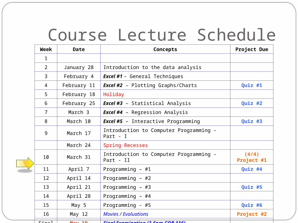
Course Lecture ScheduleWeek Date Concepts Project Due
1
2 January 28 Introduction to the data analysis
3 February 4 Excel #1 – General Techniques
4 February 11 Excel #2 – Plotting Graphs/Charts Quiz #1
5 February 18 Holiday
6 February 25 Excel #3 – Statistical Analysis Quiz #2
7 March 3 Excel #4 – Regression Analysis
8 March 10 Excel #5 – Interactive Programming Quiz #3
9 March 17 Introduction to Computer Programming - Part - I
March 24 Spring Recesses
10 March 31 Introduction to Computer Programming - Part - II (4/4) Project #1
11 April 7 Programming – #1 Quiz #4
12 April 14 Programming – #2
13 April 21 Programming – #3 Quiz #5
14 April 28 Programming – #4
15 May 5 Programming - #5 Quiz #6
16 May 12 Movies / Evaluations Project #2
Final May 19 Final Examination (3-6pm COB 116)

How do you like Scilab so far?
Great
Tool!
Outline
1. Introduction to Computer
Programming
2. More programming
4
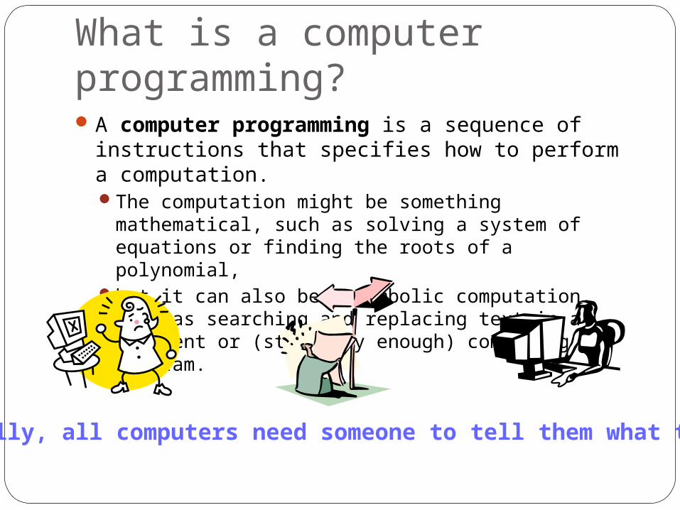
What is a computer programming? A computer programming is a sequence of
instructions that specifies how to perform a computation. The computation might be something mathematical,
such as solving a system of equations or finding the roots of a polynomial,
but it can also be a symbolic computation, such as searching and replacing text in a document or (strangely enough) compiling a program.
Basically, all computers need someone to tell them what to do!
The way of programming The single most important skill for a scientist is
problem solving. Problem solving means the ability to
formulate problems, think creatively about solutions, and express a solution clearly and accurately.
As it turns out, the process of computer programming is an excellent opportunity to practice problem-solving skills.

October, 2007
Bis 180
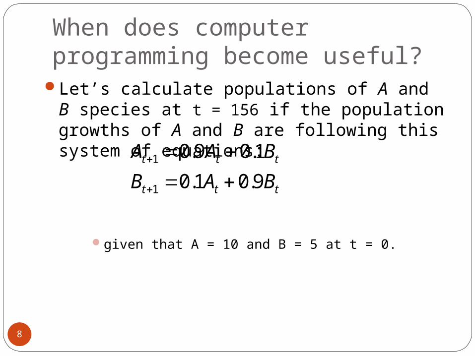
When does computer programming become useful?
Let’s calculate populations of A and B species at t = 156 if the population growths of A and B are following this system of equations:
given that A = 10 and B = 5 at t = 0.
ttt
ttt
BAB
BAA
9.01.0
1.09.0
1
1
8
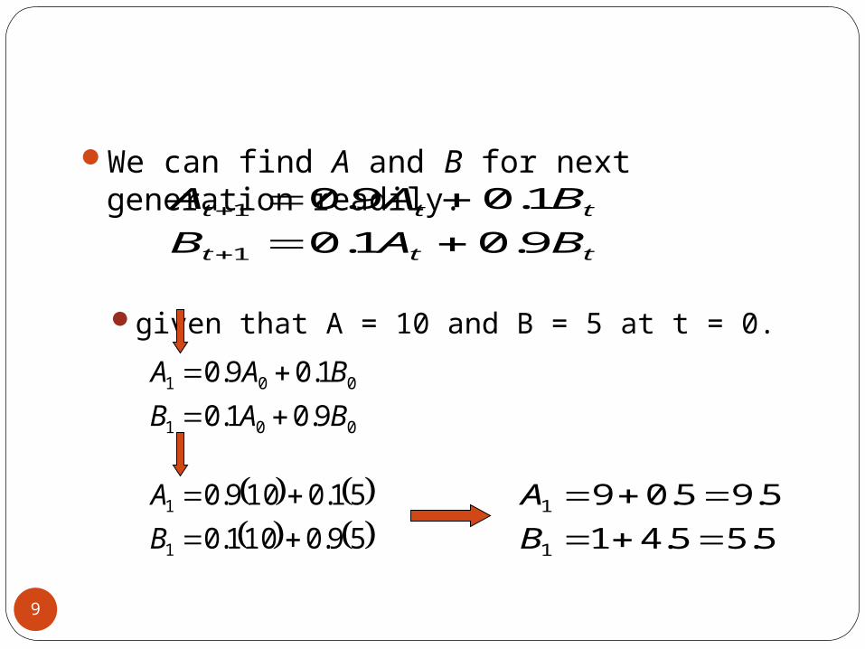
We can find A and B for next generation readily.
given that A = 10 and B = 5 at t = 0.
ttt
ttt
BAB
BAA
9.01.0
1.09.0
1
1
9
001
001
9.01.0
1.09.0
BAB
BAA
59.0101.0
51.0109.0
1
1
B
A
5.55.41
5.95.09
1
1
B
A
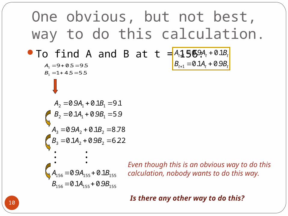
One obvious, but not best, way to do this calculation.
To find A and B at t = 156:
10
9.59.01.0
1.91.09.0
112
112
BAB
BAA
5.55.41
5.95.09
1
1
B
A
22.69.01.0
78.81.09.0
223
223
BAB
BAA
155155156
155155156
9.01.0
1.09.0
BAB
BAA
Even though this is an obvious way to do this calculation, nobody wants to do this way.
Is there any other way to do this?
ttt
ttt
BAB
BAA
9.01.0
1.09.0
1
1
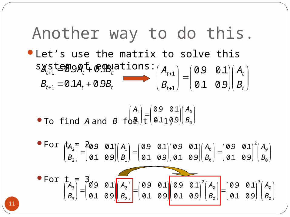
Another way to do this.Let’s use the matrix to solve this system of
equations:
To find A and B for t = 1,
For t = 2,
For t = 3,
ttt
ttt
BAB
BAA
9.01.0
1.09.0
1
1
11
t
t
t
t
B
A
B
A
9.01.0
1.09.0
1
1
0
0
1
1
9.01.0
1.09.0
B
A
B
A
0
0
2
0
0
1
1
2
2
9.01.0
1.09.0
9.01.0
1.09.0
9.01.0
1.09.0
9.01.0
1.09.0
B
A
B
A
B
A
B
A
0
0
3
0
0
2
2
2
3
3
9.01.0
1.09.0
9.01.0
1.09.0
9.01.0
1.09.0
9.01.0
1.09.0
B
A
B
A
B
A
B
A
0
0
2
0
0
1
1
2
2
9.01.0
1.09.0
9.01.0
1.09.0
9.01.0
1.09.0
9.01.0
1.09.0
B
A
B
A
B
A
B
A
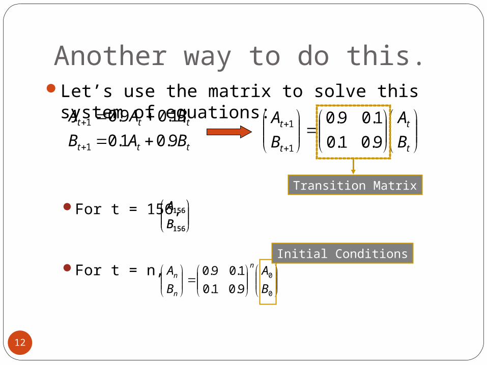
Another way to do this.Let’s use the matrix to solve this system of
equations:
For t = 156,
For t = n,
ttt
ttt
BAB
BAA
9.01.0
1.09.0
1
1
12
t
t
t
t
B
A
B
A
9.01.0
1.09.0
1
1
0
0
156
156
156
9.01.0
1.09.0
B
A
B
A
0
0
9.01.0
1.09.0
B
A
B
An
n
n
0
0
156
156
156
9.01.0
1.09.0
B
A
B
A
Transition Matrix
Initial Conditions

UC Merced
Any Questions?
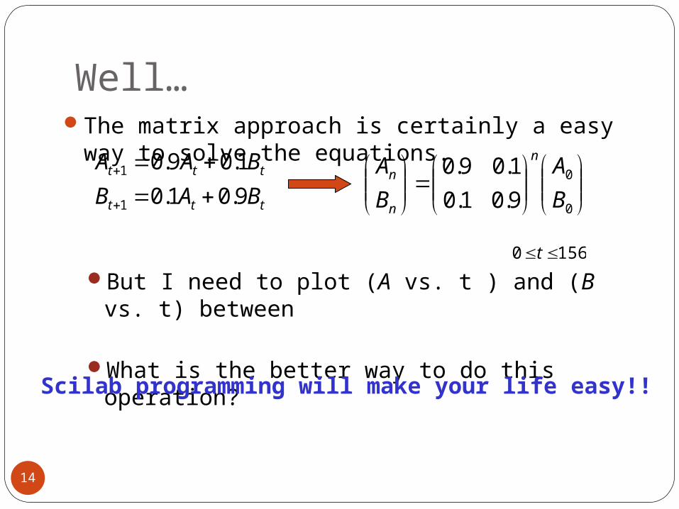
Well…The matrix approach is certainly a easy way to
solve the equations.
But I need to plot (A vs. t ) and (B vs. t) between
What is the better way to do this operation?
ttt
ttt
BAB
BAA
9.01.0
1.09.0
1
1
14
0
0
9.01.0
1.09.0
B
A
B
An
n
n
1560 t
Scilab programming will make your life easy!!
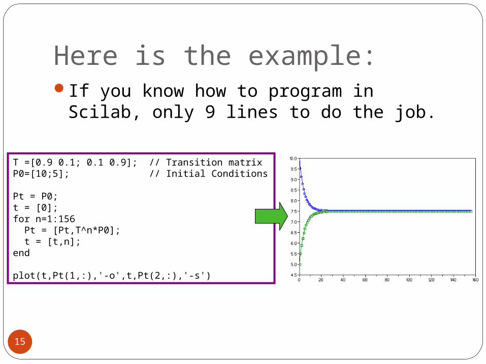
Here is the example:If you know how to program in Scilab, only
9 lines to do the job.
15
T =[0.9 0.1; 0.1 0.9]; // Transition matrixP0=[10;5]; // Initial Conditions
Pt = P0;t = [0];for n=1:156 Pt = [Pt,T^n*P0]; t = [t,n];end
plot(t,Pt(1,:),'-o',t,Pt(2,:),'-s')
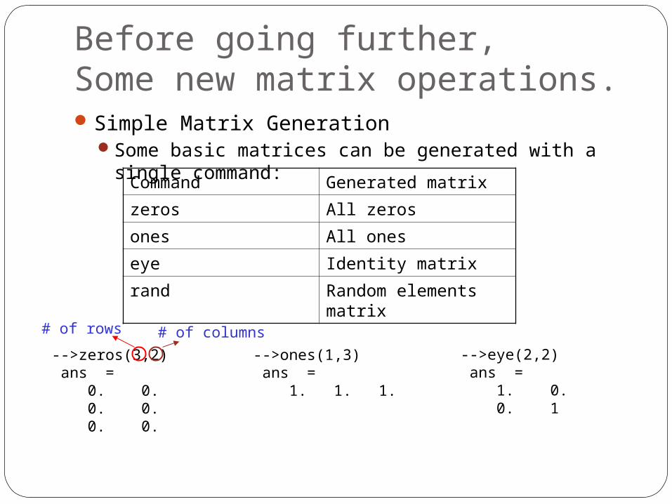
Before going further, Some new matrix operations.Simple Matrix Generation
Some basic matrices can be generated with a single command:Command Generated matrix
zeros All zeros
ones All ones
eye Identity matrix
rand Random elements matrix
-->zeros(3,2) ans = 0. 0. 0. 0. 0. 0.
# of rows # of columns
-->ones(1,3) ans = 1. 1. 1.
-->eye(2,2) ans = 1. 0. 0. 1
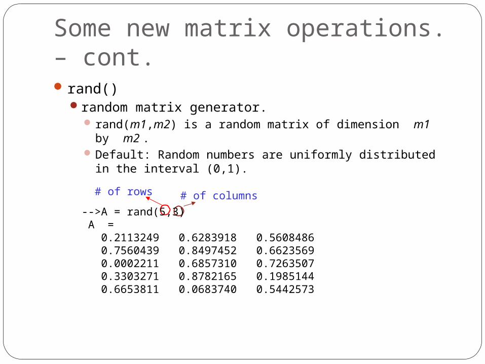
Some new matrix operations. – cont.rand()
random matrix generator. rand(m1,m2) is a random matrix of dimension m1 by
m2 . Default: Random numbers are uniformly distributed in
the interval (0,1).
# of rows # of columns
-->A = rand(5,3) A = 0.2113249 0.6283918 0.5608486 0.7560439 0.8497452 0.6623569 0.0002211 0.6857310 0.7263507 0.3303271 0.8782165 0.1985144 0.6653811 0.0683740 0.5442573
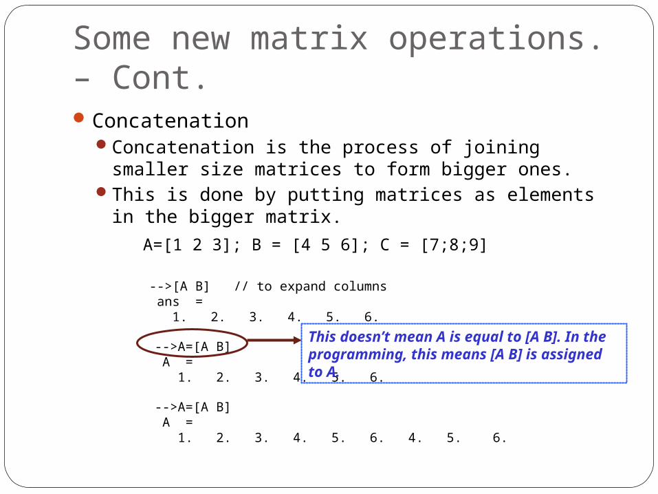
Some new matrix operations. – Cont.Concatenation
Concatenation is the process of joining smaller size matrices to form bigger ones.
This is done by putting matrices as elements in the bigger matrix.
A=[1 2 3]; B = [4 5 6]; C = [7;8;9]
-->[A B] // to expand columns ans = 1. 2. 3. 4. 5. 6.
-->A=[A B] A = 1. 2. 3. 4. 5. 6.
-->A=[A B] A = 1. 2. 3. 4. 5. 6. 4. 5. 6.
This doesn’t mean A is equal to [A B]. In the programming, this means [A B] is assigned to A.
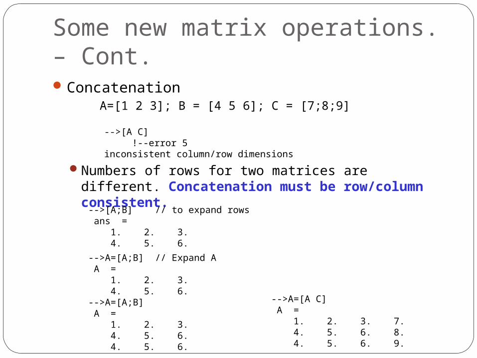
Some new matrix operations. – Cont.Concatenation
Numbers of rows for two matrices are different. Concatenation must be row/column consistent.
A=[1 2 3]; B = [4 5 6]; C = [7;8;9]
-->[A C] !--error 5inconsistent column/row dimensions
-->[A;B] // to expand rows ans = 1. 2. 3. 4. 5. 6.
-->A=[A;B] // Expand A A = 1. 2. 3. 4. 5. 6.-->A=[A;B] A = 1. 2. 3. 4. 5. 6. 4. 5. 6.
-->A=[A C] A = 1. 2. 3. 7. 4. 5. 6. 8. 4. 5. 6. 9.

UC Merced
Any Questions?
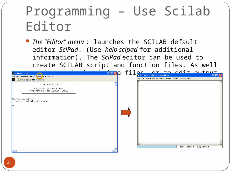
Programming – Use Scilab Editor The "Editor" menu : launches the SCILAB default editor
SciPad. (Use help scipad for additional information). The SciPad editor can be used to create SCILAB script and function files. As well as to create input data files, or to edit output data files.
21
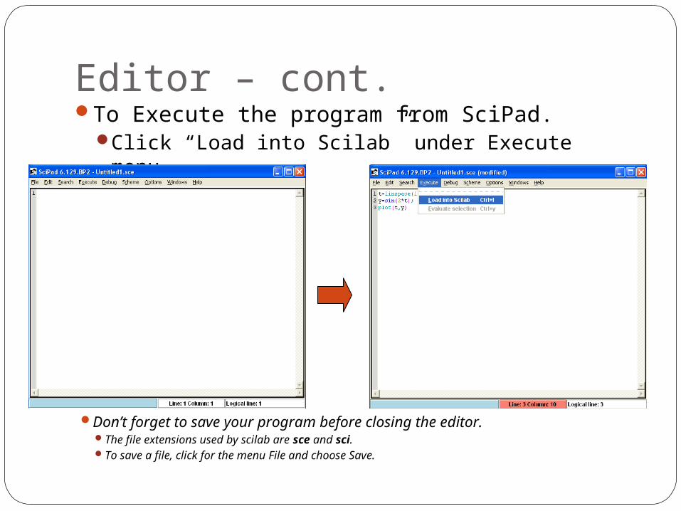
Editor – cont.To Execute the program from SciPad.
Click “Load into Scilab” under Execute menu.
Don’t forget to save your program before closing the editor.The file extensions used by scilab are sce and sci.To save a file, click for the menu File and choose Save.
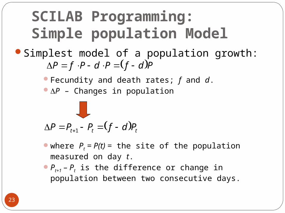
SCILAB Programming: Simple population Model
Simplest model of a population growth:
Fecundity and death rates; f and d.P – Changes in population
where Pt = P(t) = the site of the population measured on day t.
Pt+1 – Pt is the difference or change in population between two consecutive days.
23
PdfPdPfP
ttt PdfPPP 1
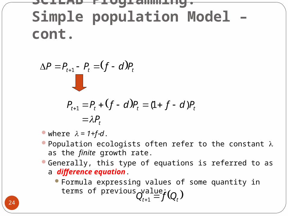
SCILAB Programming: Simple population Model – cont.
where = 1+fd. Population ecologists often refer to the constant as the finite growth
rate.Generally, this type of equations is referred to as a
difference equation.Formula expressing values of some quantity in terms
of previous value:24
ttt PdfPPP 1
t
tttt
P
PdfPdfPP
)1(1
tt QfQ 1
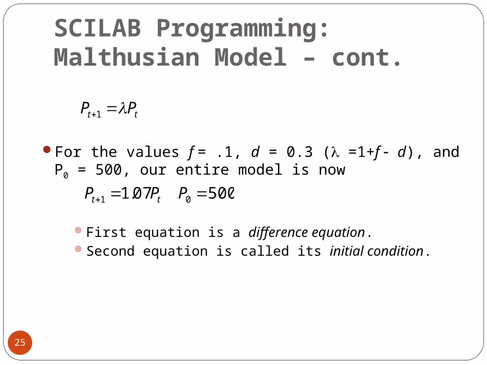
SCILAB Programming: Malthusian Model – cont.
For the values f = .1, d = 0.3 ( =1+f d), and P0 = 500, our entire model is now
First equation is a difference equation.Second equation is called its initial condition.
25
tt PP 1
50007.1 01 PPP tt
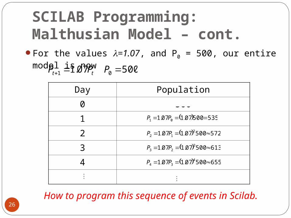
SCILAB Programming: Malthusian Model – cont.
For the values =1.07, and P0 = 500, our entire model is now
26
50007.1 01 PPP tt
Day Population
0 500
1
2
3
4
53550007.107.1 01 PP
57250007.107.1 212 PP
61350007.107.1 323 PP
65550007.107.1 434 PP
How to program this sequence of events in Scilab.
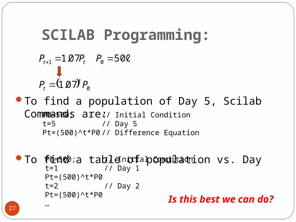
SCILAB Programming:
To find a population of Day 5, Scilab Commands are:
To find a table of population vs. Day
27
50007.1 01 PPP tt
007.1 PP tt
P0=500; // Initial Conditiont=5 // Day 5 Pt=(500)^t*P0 // Difference Equation
P0=500; // Initial Conditiont=1 // Day 1 Pt=(500)^t*P0t=2 // Day 2 Pt=(500)^t*P0… Is this best we can do?
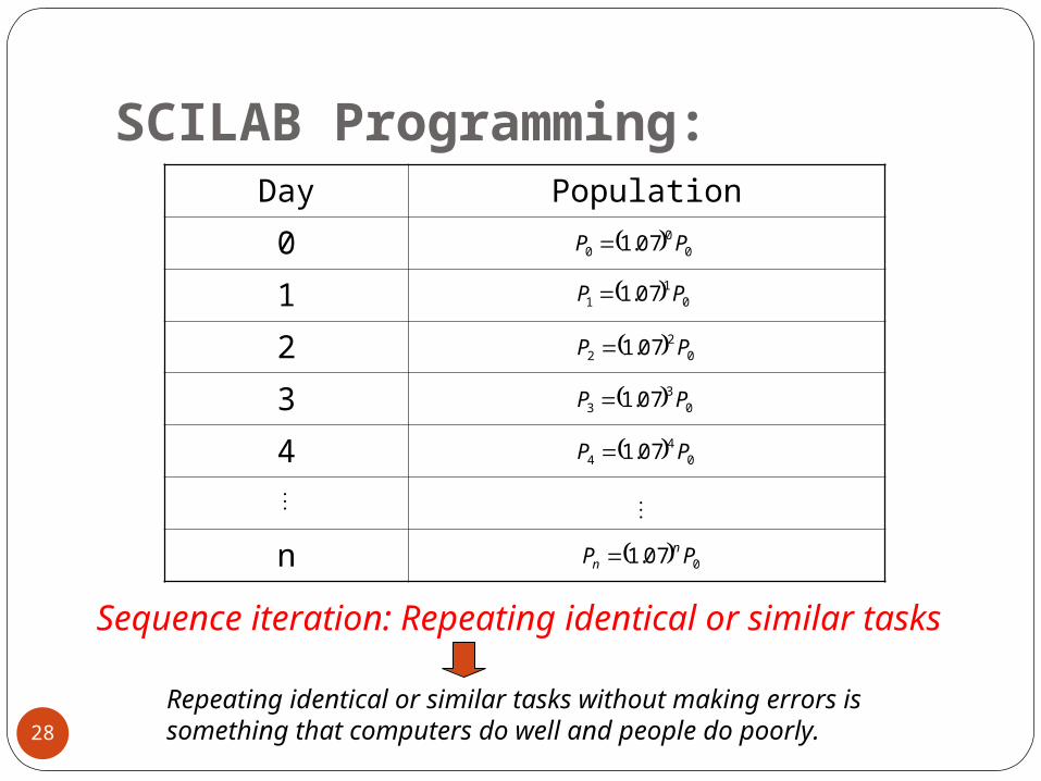
SCILAB Programming:
28
Day Population
0
1
2
3
4
n
01
1 07.1 PP
02
2 07.1 PP
03
3 07.1 PP
04
4 07.1 PP
Sequence iteration: Repeating identical or similar tasks
007.1 PP nn
00
0 07.1 PP
Repeating identical or similar tasks without making errors is something that computers do well and people do poorly.
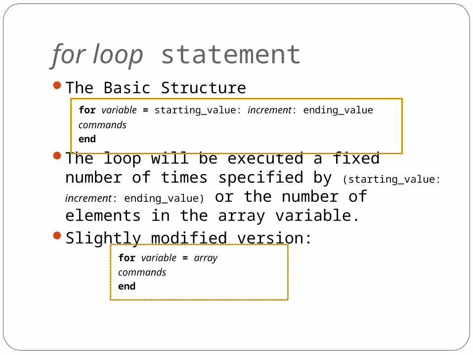
for loop statementThe Basic Structure
for variable = starting_value: increment: ending_value
commands
end
The loop will be executed a fixed number of times specified by (starting_value: increment:
ending_value) or the number of elements in the array variable.
Slightly modified version:for variable = array
commands
end
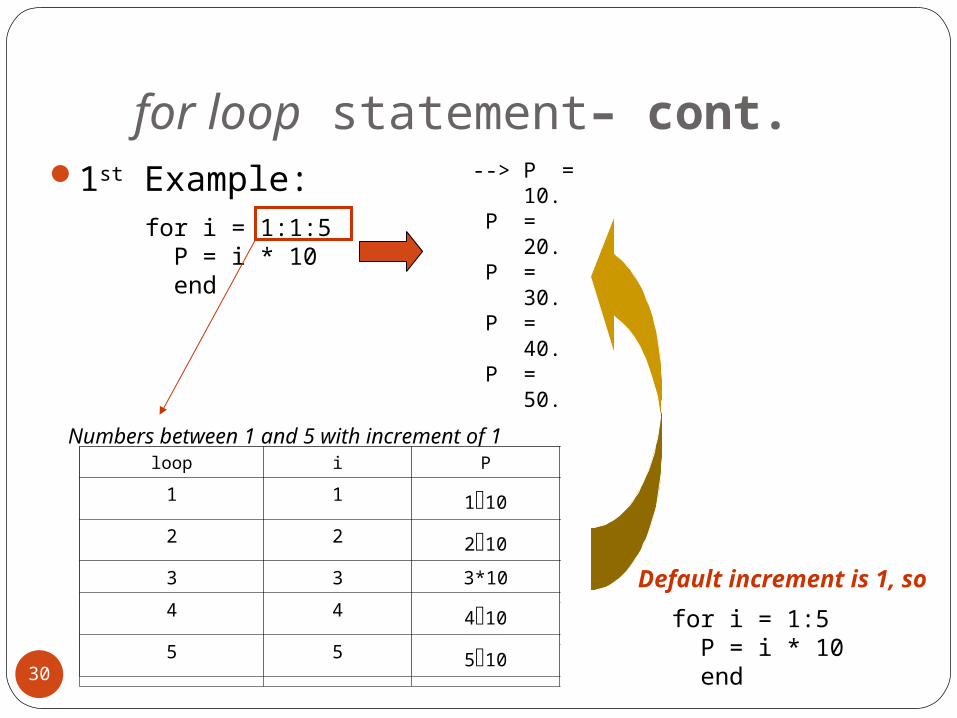
for loop statement– cont.1st Example:
30
for i = 1:1:5 P = i * 10 end
--> P = 10. P = 20. P = 30. P = 40. P = 50.
loop i P
1 1 110
2 2 210
3 3 310
4 4 410
5 5 510
Numbers between 1 and 5 with increment of 1loop i P
1 1 110
2 2 210
3 3 3*10
4 4 410
5 5 510
for i = 1:5 P = i * 10 end
Default increment is 1, so
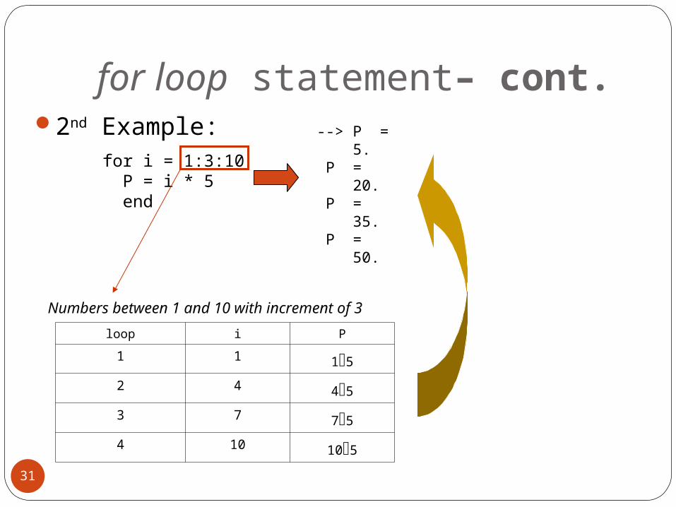
for loop statement– cont.2nd Example:
31
for i = 1:3:10 P = i * 5 end
--> P = 5. P = 20. P = 35. P = 50.
loop i P
1 1 15
2 4 45
3 7 75
4 10 105
Numbers between 1 and 10 with increment of 3
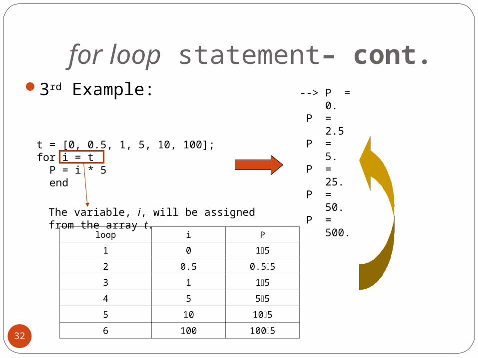
for loop statement– cont.3rd Example:
32
t = [0, 0.5, 1, 5, 10, 100];for i = t P = i * 5 end
--> P = 0. P = 2.5 P = 5. P = 25. P = 50. P = 500. loop i P
1 0 15
2 0.5 0.55
3 1 15
4 5 55
5 10 105
6 100 1005
The variable, i, will be assigned from the array t.
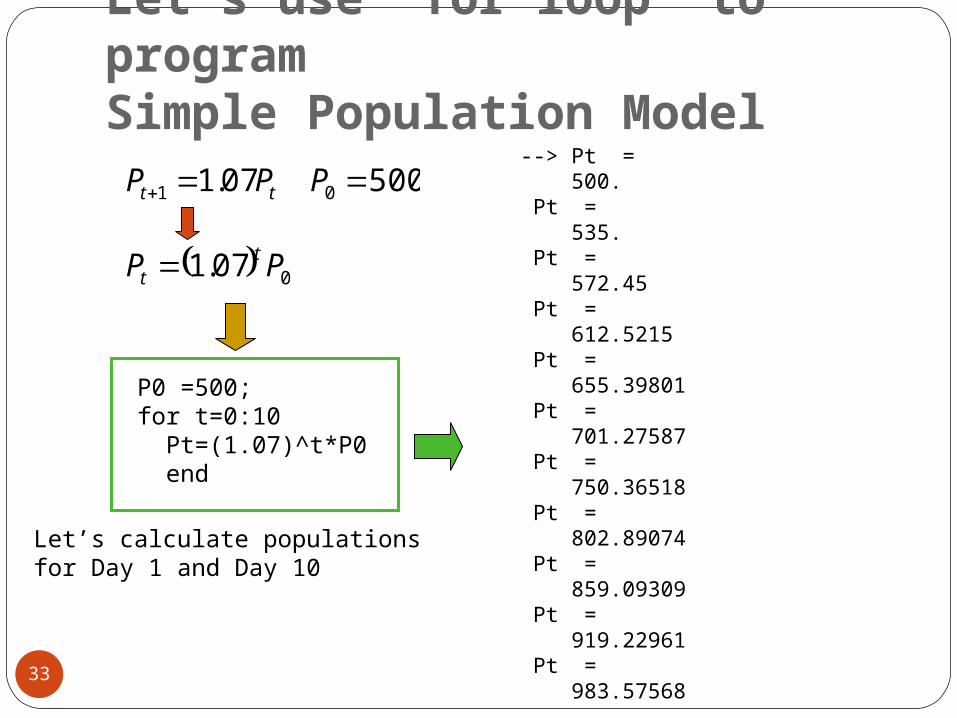
Let’s use “for loop” to program Simple Population Model
33
50007.1 01 PPP tt
007.1 PP tt
P0 =500;for t=0:10 Pt=(1.07)^t*P0 end
--> Pt = 500. Pt = 535. Pt = 572.45 Pt = 612.5215 Pt = 655.39801 Pt = 701.27587 Pt = 750.36518 Pt = 802.89074 Pt = 859.09309 Pt = 919.22961 Pt = 983.57568
Let’s calculate populations for Day 1 and Day 10
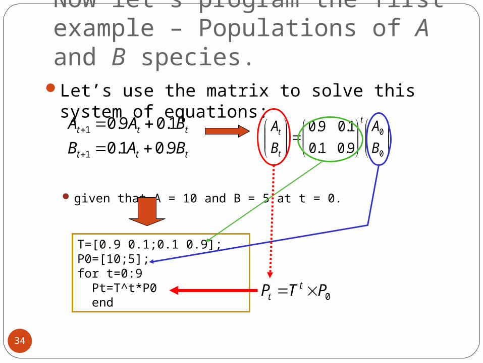
Now let’s program the first example – Populations of A and B species.
Let’s use the matrix to solve this system of equations:
given that A = 10 and B = 5 at t = 0.
ttt
ttt
BAB
BAA
9.01.0
1.09.0
1
1
34
0
0
9.01.0
1.09.0
B
A
B
At
t
t
T=[0.9 0.1;0.1 0.9];P0=[10;5];for t=0:9 Pt=T^t*P0 end 0PTP t
t
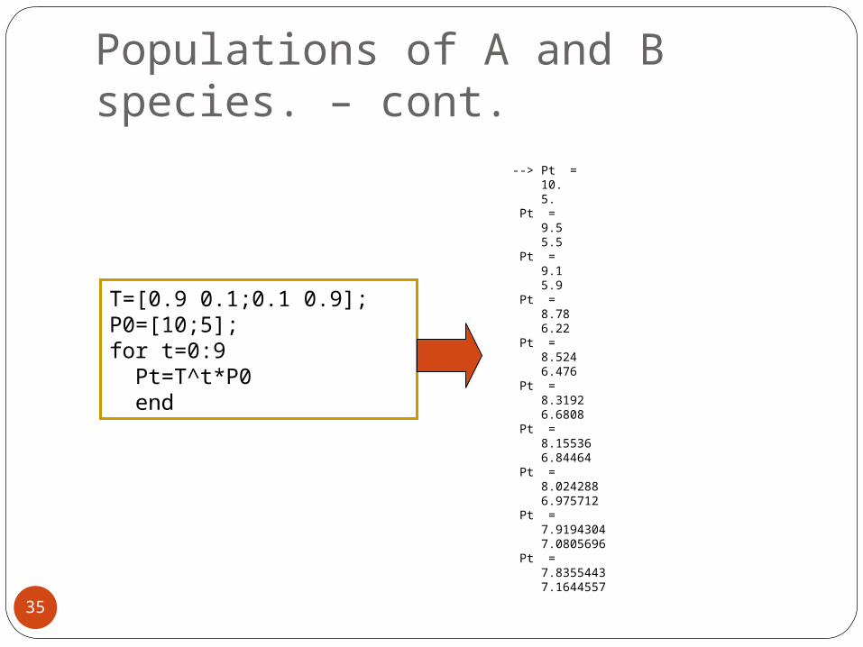
Populations of A and B species. – cont.
35
--> Pt = 10. 5. Pt = 9.5 5.5 Pt = 9.1 5.9 Pt = 8.78 6.22 Pt = 8.524 6.476 Pt = 8.3192 6.6808 Pt = 8.15536 6.84464 Pt = 8.024288 6.975712 Pt = 7.9194304 7.0805696 Pt = 7.8355443 7.1644557
T=[0.9 0.1;0.1 0.9];P0=[10;5];for t=0:9 Pt=T^t*P0 end

UC Merced
Any Questions?
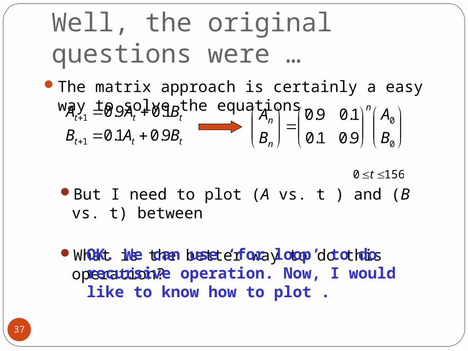
Well, the original questions were …
The matrix approach is certainly a easy way to solve the equations.
But I need to plot (A vs. t ) and (B vs. t) between
What is the better way to do this operation?
ttt
ttt
BAB
BAA
9.01.0
1.09.0
1
1
37
0
0
9.01.0
1.09.0
B
A
B
An
n
n
1560 t
OK. We can use ‘for loop’ to do recursive operation. Now, I would like to know how to plot .
T =[0.9 0.1; 0.1 0.9]; // Transition matrixP0=[10;5]; // Initial Conditions
Pt = P0;t = [0];for n=1:156 Pt = [Pt,T^n*P0]; t = [t,n];end
plot(t,Pt(1,:),'-o',t,Pt(2,:),'-s')
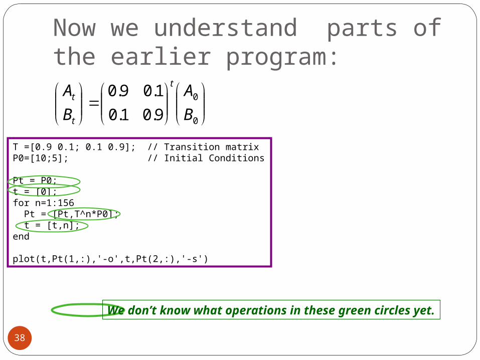
Now we understand parts of the earlier program:
0
0
9.01.0
1.09.0
B
A
B
At
t
t
38
We don’t know what operations in these green circles yet.
T =[0.9 0.1; 0.1 0.9]; // Transition matrixP0=[10;5]; // Initial Conditions
Pt = P0;t = [0]for n=1:156 Pt = [Pt,T^n*P0]; t = [t,n]end
plot(t,Pt(1,:),'-o',t,Pt(2,:),'-s')
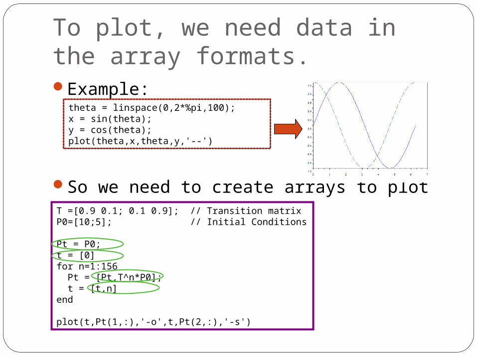
To plot, we need data in the array formats.Example:
So we need to create arrays to plot
theta = linspace(0,2*%pi,100);x = sin(theta);y = cos(theta);plot(theta,x,theta,y,'--')
T =[0.9 0.1; 0.1 0.9]; // Transition matrixP0=[10;5]; // Initial Conditions
Pt = P0;
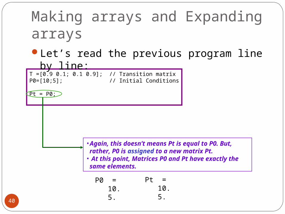
Making arrays and Expanding arrays
40
• Again, this doesn’t means Pt is equal to P0. But, rather, P0 is assigned to a new matrix Pt.
• At this point, Matrices P0 and Pt have exactly the same elements.
Let’s read the previous program line by line:
P0 = 10. 5.
Pt = 10. 5.
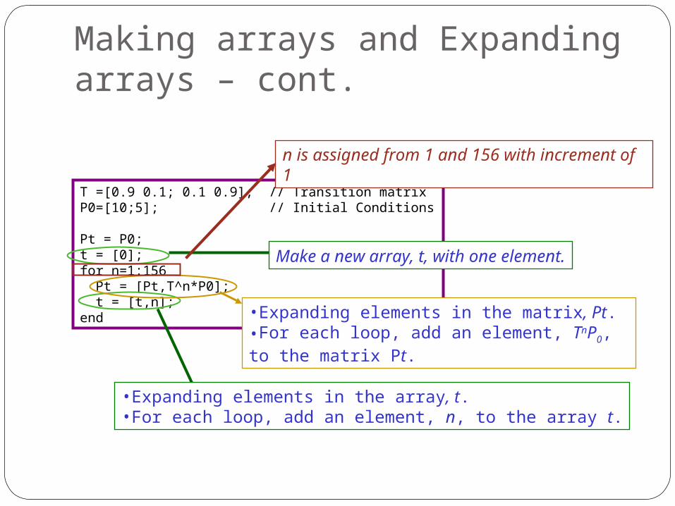
Making arrays and Expanding arrays – cont.
T =[0.9 0.1; 0.1 0.9]; // Transition matrixP0=[10;5]; // Initial Conditions
Pt = P0;t = [0];for n=1:156 Pt = [Pt,T^n*P0]; t = [t,n];end
Make a new array, t, with one element.
•Expanding elements in the array, t.•For each loop, add an element, n, to the array t.
•Expanding elements in the matrix, Pt.•For each loop, add an element, TnP0, to the matrix Pt.
n is assigned from 1 and 156 with increment of 1
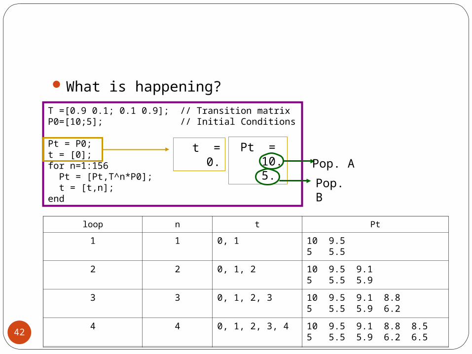
What is happening?
T =[0.9 0.1; 0.1 0.9]; // Transition matrixP0=[10;5]; // Initial Conditions
Pt = P0;t = [0];for n=1:156 Pt = [Pt,T^n*P0]; t = [t,n];end
42
t = 0.
Pt = 10. 5.
loop n t Pt
1 1 0, 1 10 9.55 5.5
2 2 0, 1, 2 10 9.5 9.15 5.5 5.9
3 3 0, 1, 2, 3 10 9.5 9.1 8.85 5.5 5.9 6.2
4 4 0, 1, 2, 3, 4 10 9.5 9.1 8.8 8.55 5.5 5.9 6.2 6.5
Pop. A
Pop. B
loop n t Pt
1 1 0, 1 10 9.55 5.5
2 2 0, 1, 2 10 9.5 9.15 5.5 5.9
3 3 0, 1, 2, 3 10 9.5 9.1 8.85 5.5 5.9 6.2
4 4 0, 1, 2, 3, 4 10 9.5 9.1 8.8 8.55 5.5 5.9 6.2 6.5
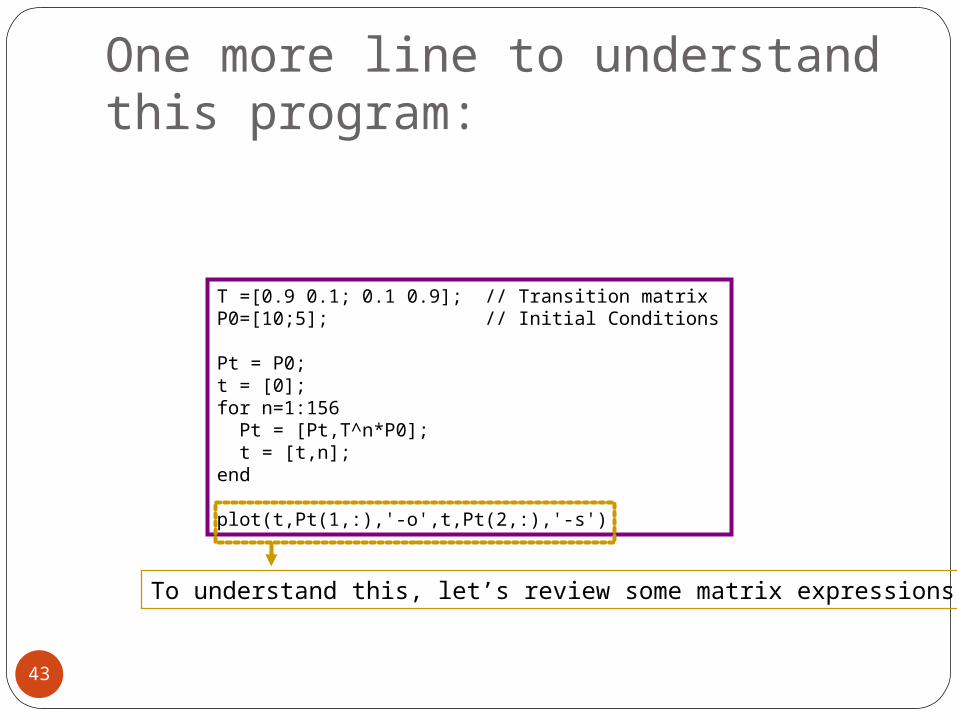
T =[0.9 0.1; 0.1 0.9]; // Transition matrixP0=[10;5]; // Initial Conditions
Pt = P0;t = [0];for n=1:156 Pt = [Pt,T^n*P0]; t = [t,n];end
plot(t,Pt(1,:),'-o',t,Pt(2,:),'-s')
One more line to understand this program:
43
To understand this, let’s review some matrix expressions.
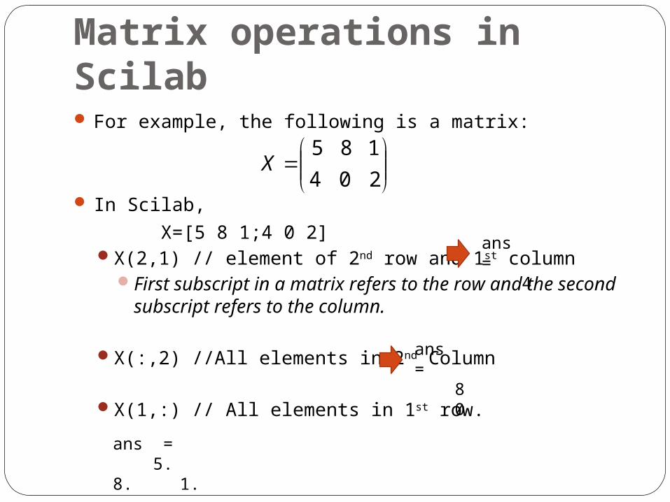
Matrix operations in Scilab For example, the following is a matrix:
In Scilab,
X=[5 8 1;4 0 2]X(2,1) // element of 2nd row and 1st column
First subscript in a matrix refers to the row and the second subscript refers to the column.
X(:,2) //All elements in 2nd Column
X(1,:) // All elements in 1st row.
204
185X
ans = 5. 8.
1.
ans = 8 0
ans = 4
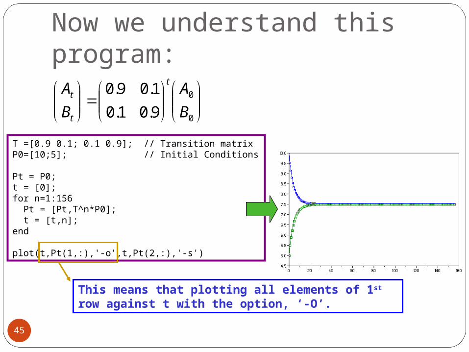
T =[0.9 0.1; 0.1 0.9]; // Transition matrixP0=[10;5]; // Initial Conditions
Pt = P0;t = [0];for n=1:156 Pt = [Pt,T^n*P0]; t = [t,n];end
plot(t,Pt(1,:),'-o',t,Pt(2,:),'-s')
Now we understand this program:
0
0
9.01.0
1.09.0
B
A
B
At
t
t
45
This means that plotting all elements of 1st row against t with the option, ‘-O’.

UC Merced46
Any Questions?
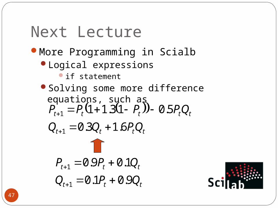
Next LectureMore Programming in Scialb
Logical expressionsif statement
Solving some more difference equations, such as
47
tttt
ttttt
QPQQ
QPPPP
6.13.0
5.013.11
1
1
ttt
ttt
QPQ
QPP
9.01.0
1.09.0
1
1
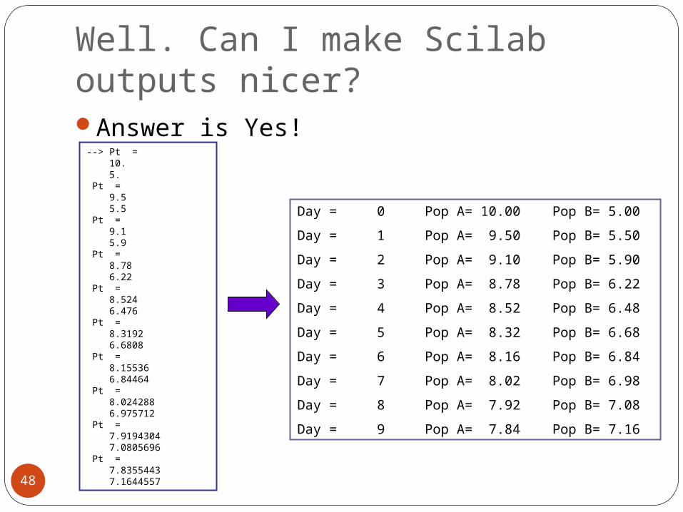
Well. Can I make Scilab outputs nicer?Answer is Yes!
48
--> Pt = 10. 5. Pt = 9.5 5.5 Pt = 9.1 5.9 Pt = 8.78 6.22 Pt = 8.524 6.476 Pt = 8.3192 6.6808 Pt = 8.15536 6.84464 Pt = 8.024288 6.975712 Pt = 7.9194304 7.0805696 Pt = 7.8355443 7.1644557
Day = 0 Pop A= 10.00 Pop B= 5.00
Day = 1 Pop A= 9.50 Pop B= 5.50
Day = 2 Pop A= 9.10 Pop B= 5.90
Day = 3 Pop A= 8.78 Pop B= 6.22
Day = 4 Pop A= 8.52 Pop B= 6.48
Day = 5 Pop A= 8.32 Pop B= 6.68
Day = 6 Pop A= 8.16 Pop B= 6.84
Day = 7 Pop A= 8.02 Pop B= 6.98
Day = 8 Pop A= 7.92 Pop B= 7.08
Day = 9 Pop A= 7.84 Pop B= 7.16