1

Math 280 Calculus III Chapter 13 Vector-Valued Functions

Sections: 13.1, 13.2 13.3, 13.4 Topics:…

…

Vector Functions and Space Curves Derivatives and Integrals of Vector Functions

Arc Length and Curvature Motion in Space: Velocity and Acceleration

Section 13.1 Vector Functions and Space Curves

A vector-valued function, or vector function, is a function of the form

. Such a function has a domain that is a set of real numbers and has a range that is a set of vectors. So the function maps a real number input to a vector output.

Each of the functions f(t), g(t), and h(t) are real-valued functions called the component

functions of r(t). The variable t is commonly used because of how often the independent variable turns out to be time in application problems.

The limit of a vector function is defined by taking the limits of its component functions as shown in the following example.

We can define the derivative as an extension of the delta-epsilon argument presented in Calculus I.

In practice, we will focus on the component definition, not the formal definition.

On the next page is the component definition of the limit of a vector function.

2

Figure 13.1 represents the general idea of a vector function. Figures 13.2 and 13.3 are examples of vector functions and their graphs.

(See figure 13.3 above.)

Figure 13.2 is on the next page.

3

A vector function of the form is also known as a

parametric equation. The variable t is called the parameter.

A good method to use when sketching parametric equations in space is to look at slices on each of the two-variable planes. For example, for the vector function

r(t) = cos t i + sin t j + t k, the image on the xy-plane is the two-dimensional image r(t) = cos t i + sin t j which is a circle. The yz-plane is a sine curve and the xz-plane is a cosine curve. When we combine each of these we get the sketch below.

We will use computer algebra systems (CAS) to generate such graphs later in the course.

4

Example Find a vector equation and parametric equations for the line segment that joins the point P(1, 3, -2) to the point Q(2, -1, 3). Example Find a vector function that represents the curve of intersection of the two surfaces.

The paraboloid � = 4�� + �� and the parabolic cylinder y = x 2.

Example

Find the domain of the vector function. r(t) = cos t i + �

�j + √4− �� k

5

Example

(a) All the space curves shown in figures 13.2 are continuous because their component functions are continuous at every value of t in �−∞, ∞�.

(b) The function

���� = �cos ��� + �sin ��� + 1��� + 3��� − 1� �

is discontinuous at every integer that is undefined on the h(t) function where h(t) is undefined and so also discontinuous. (c) The function

���� = �cos ��� + � 1�� + 2��� − 2��� + 1

��� + 3��� − 1� �

is discontinuous at all the point ��{2, −2, 0, −3, 1}. The idea here is that if a point is discontinuous for even one value of x on any component function, then the entire vector function is discontinuous at that value of x.

Example Find the limit.

lim%→' (�� − �� − 1 � + √� + 8 � + sin * �

ln � �+

6

Section 13.2 Derivatives and Integrals of Vector Functions

The derivative r'(t) of a vector function r is defined in much the same way as for

real- valued functions:

Proof of the component form of the derivative of a vector function.

7

As shown in the figures below, the derivative of a vector function can be used to find a tangent vector to the curve. Since the tangent is itself a vector, there are many such vectors, each having a different length, but all following the same line. So in space, we find a special case of all the tangent vectors. We call this vector the unit tangent vector.

,��� � -′���|-′���|

Example

Find the derivative of the vector function. r(t) = ⟨��, �1⟩, t = 1

8

Proof of the vector function chain rule (Rule 7).

9

Integration of Vector Functions

Note that each component function has an unknown constant value. HOWEVER, each unknown constant is associated with a specific component (either i or j or k). When we factor out these three constant terms we can combine then to get a constant vector, C. This leads to the definition below.

Proof of the above definition.

10

We can extend the Fundamental Theorem of Calculus to continuous vector functions as

follows:

3 -���4� � 5���|6

789 � 5�8� − 5�9�

where R(t) is the antiderivative of r(t). This allows us to evaluate definite integrals involving vector functions.

Example

Find the unit tangent vector T(t) at the point with the given value of the parameter t.

r(t) = ( t 3 + 3t, t 2 + 1, 3t + 4 ), t = 1

11

Example Find parametric equations for the tangent line to the curve with the given parametric equations

at the specified point.

x = e t, y = te t, z= �:�;; (1, 0, 0)

12

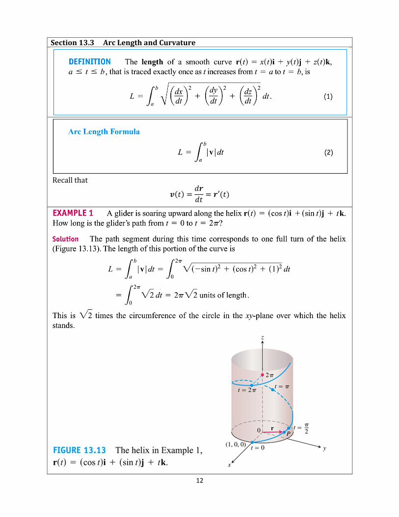
Section 13.3 Arc Length and Curvature

Recall that

<��� � 4-4� � -′���

13

So far all of the vector functions have been in terms of the independent variable t, which allows the function to define a location in space after t – amount of time has passed. We often want to define the location in space in terms of how far the object has traveled along the path of travel. To do this, we must reparametrize. Suppose that C is a curve given by a vector function

r(t) = f (t) i + t(t) j + h(t) k a < t < b

where r' is continuous and C is traversed exactly once as t increases from a to b. We define

its arc length function s by

If we differentiate both sides of this equation we get

4=4� � |-′���|

In this case, the time, t, no longer parametrizes

the function. Only when the speed is constant

does the s-parameter and the t-parameter agree.

Example 2 Reparametrize the helix r(t) = cos t i + sin t j + t k with respect to arc length measured from (1, 0, 0) in the direction of increasing t.

14

Curvature

A parametrization r(t) is called smooth on an interval I if r’ is continuous and >?��� @ 0 on I. A curve is called smooth if it has a smooth parametrization. A smooth curve has no sharp corners or cusps; when the tangent vector turns, it does so continuously. If C is a smooth curve defined by the vector function r, recall that the unit tangent vector T(t) is given by

,��� � -′���|-′���|

The curvature is easier to compute if it is expressed in terms of the parameter t instead of s, so we use the Chain Rule to write

4,4� � 4,

4= ∙ 4=4� B = C4,

4=C = D4,4� DD4=4�D

Since

EFE� � |-′���|, we get B��� �

GHI���G|JI���| .

Alternatively, the curvature of the curve given by the vector function r is

B��� � GJI���KJII���G

|JI���|L

Proof

15

Example 3

A straight line is parameterized by r(t) = C + tv for constant vectors C and v. Thus, r’(t) =

v, and the unit tangent vector , � <|<| is a constant vector that always points in the same

direction and has derivative 0. It follows that, for any value of the parameter t, the

curvature of the straight line is

M � 1|<| C4,

4� C � 1|<| |N| � 0.

Example 4 Let’s find the curvature of a circle. We start with the parameterization of a

circle of radius a.

-��� � �9 cos ��� + �9 sin ���

16

Example 5

Find the curvature of the twisted cubic -��� � ⟨�, ��, �1⟩

(a) at a general point. (b) at the point (0, 0, 0).

When we have a simple plane curve defined by y = f(x), then we can derive the formula

B��� � GPII���G

|Q�PI�R��;|L/;

Example 6 Find the curvature of the parabola y = x2 at the points (0, 0), (1, 1), and (2, 4).

17

The Normal and Binormal Vectors

To each tangent vector there is a plane that is orthogonal to T(t) and which contains infinitely many vectors that form right angles with T(t). However, only one of these vectors is in the same direction as the derivative of T(t). We will define the unit vector in the direction of T’(t) as the Normal vector and denote it as N(t). Below is a proof that the derivative T’(t) is indeed orthogonal to T(t). We will then define N(t) as the unit vector in the direction of T’(t). Note that if |-���| is a constant, then -′��� is orthogonal to r(t) for all t. Proof We know -��� ∙ -��� � |-���|� � T� and we know c2 is a constant. So we get

0 � 44� U-��� ∙ -���V � -?��� ∙ -��� + -��� ∙ -′��� = 2-′��� ∙ -���

So -?��� ∙ -��� � 0 which says that -?��� is orthogonal to -���. ⎕ From the notes above, we have

W��� � ,′���|,′���|

We now add one more vector related to the motion of a particle in space. Note that the unit tangent vector and the normal vector both have initial positions at the location of the particle at time, t. Recall that two vectors in space with a common initial point must lie in a plane. We can define this plane using the cross-product and the resulting vector defines the plane by being orthogonal to the plane.

Thus, the binormal is defined as X��� � ,��� K W��� and thus defines the plane that contains both T and N.

18

Example 7 Find the unit tangent, unit normal and binormal vectors for the circular helix -��� � cos �� + sin �� + �� Example 8 Find the equations of the normal plane and osculating plane of the helix in example 7

above at the point �0, 1, Y��.

Example 9 Find and graph the osculating circle of the parabola y = x2 at the origin.

19

Section 13.4 Motion in Space: Velocity and Acceleration

Suppose a particle moves through space so that its position vector at time t is rt . Notice from Figure 1 that, for small values of h, the vector

The vector (1) above gives the average velocity over a time interval of length h and its limit is the velocity vector, v(t), at time t.

<��� � limZ→N(>�� � [� >���

[ + � -′��� The velocity vector is also the tangent vector and points in the direction of the tangent line. The speed of the particle at time t is the magnitude of the velocity vector and in this respect is not related to the unit tangent vector. To calculate the speed, we can find

|\���| � |>′���| � 4=4� � >9�:]^T[9_`:�4a=�9_T:�ba�[>:=c:T��]�ad:

Acceleration is the rate of change in the velocity with respect to time. Using this notion,

we can define acceleration, a(t), as |\���| � |>′���| � EFE�

<<<<<< Intuitively explanation of acceleration

20

Example 1 The position vector of an object moving in a plane is given by -��� � �1� + ���. Find its velocity, speed, and acceleration when t = 1 and illustrate geometrically. Example 2 Find the velocity, acceleration, and speed of a particle with position vector >��� � ⟨��, :�, �:�⟩.

21

Example 3 A moving particle starts at an initial position >�0� � ⟨1, 0, 0⟩ with initial velocity <�0� � � � � �. Its acceleration is e��� � 4�� 6�� � �. Find its velocity and position at time t.

22

In physics, force = mass times acceleration. In space geometry and using vector functions, we can define force as g��� � de��� In this formula, F and a are vector functions while m is either a constant or (beyond what we will see) a scalar function. An example of when m needs to be a scalar function is the path of a comet which is constantly losing mass but at varying rates. We may wish to find the force of impact of such a comet. Example 4 An object with mass m that moves in a circular path with constant angular speed, h has position vector -��� � 9 cos h� � � 9 sin h� �. Find the force acting on the object and show that it is directed toward the origin.

23

Example 5 A projectile is fired with angle of elevation i and initial velocity vo. (See the figure.) Assuming that air resistance is negligible and the only external force is due to gravity, find the position function, r(t), of the projectile. What value of i maximizes the range?

24

Example 6 A projectile is fired with an initial speed of 200 m/s and an initial height of 100m with an angle of elevation 60 degrees. Find (a) the range of the projectile, (b) the maximum height reached, and (c) the speed at impact.

25

Tangential and Normal Components of Acceleration

Intuitively, we know that the velocity vector can be found by multiplying the scalar magnitude of speed times the direction vector T(t), which is the unit tangent vector. We have defined speed as |\���|, but in our situation, we would not know the velocity vector, so we will call the speed v. Thus, we get the formula <��� � \,���.

We can verify this using known formulas. We know that

,��� � -′(�)|-′(�)|

=<(�)|<(�)|

=<(�)\

If we solve for v(t), we get the formula above.

Now differentiate both sides of this equation to get

44�<(�) =

44�[\,(�)]

which yields the equation

e = <? = \?, + \,′.

We are trying to define the acceleration, a, in terms of tangential, T, and normal, N, components. So we need to change the form above until the two components are NOT T and T’, but T and N instead. To accomplish this, we will make some substitutions that are already known to us.

We know that B(�) = GHI(�)G

|JI(�)| (see page 14 in the notes above).

Using v = |>?(�)| we get |j?(�)| = B\. Also, we know that W(�) = ,?(�)|,?(�)|.

Substituting, we get j?(�) = W(�)|,′(�)| = B\W(�).

Above, we had the formula e = \?, + \,′. If we substitute for T’, we get the desired equation

e(�) = \?,(�) + \B\W(�). Simplifying, we get

e = \?, + B\�W.

Since we now have scalar values defined as the magnitudes of the T and the N directions, we simply define the tangential component, 9H , as the appropriate component above, which is v’. And we define the normal component, 9k, as the appropriate component above, B\�. This gives us the formula

e = 9H, +9kW

where 9H = \? and 9k = B\�. Both of these components are scalars and only make sense on the curve when they are multiplied by the Tangential and Normal vectors.

26

Example 7 Find the tangential and normal components of the acceleration vector for the vector function

-(�) = �� + ��� + 3��